Supporting Information for:

"Rheological Link Between Polymer Melts

with a High Molecular Weight Tail and

Enhanced Formation of Shish-Kebabs"

Sara Lindeblad Wingstrand,† Bo Shen,‡ Julie A. Korn�eld,‡ Kell Mortensen,¶

Daniele Parisi,§,‖ Dimitris Vlassopoulos,§,‖ and Ole Hassager∗,†

†Technical University of Denmark, Department of Chemical and Biochemcial Engineering,

Danish Polymer Center,DK-2800 Kgs. Lyngby, Denmark

‡California Institute of Technology, Division of Chemistry and Chemical Engineering,

Pasadena, CA 91125, USA

¶University of Copenhagen, Niels Bohr Institute, X-ray and Neutron Science, DK-2100

København Ø, Denmark

§Institute of Electronic Structure and Laser, FORTH, Heraklion 71110, Crete Greece

‖Department of Materials Science & Technology, University of Crete, Heraklion 71003,

Crete Greece

E-mail: oh@kt.dtu.dk

1

Supplemental Text

Details on Rheological measurements

Creep The samples were shaped into discotic specimens at 150C using a home-made vac-

uum press mold for twenty minutes and then loaded on the rheometer at the same tempera-

ture. We used a stress-controlled rheometer MCR702 (Anton Paar, Austria). The specimen

was placed between two stainless steel parallel plates of 8 mm diameter and gap about 0.7

mm, calibrated for thermal expansion. Temperature control was achieved by means of a hy-

brid temperature control system CTD180 which has intermediate characteristics between a

Peltier cell and a convection oven. All tests were performed in nitrogen atmosphere in order

to reduce the risk of sample degradation. The measurement protocol consisted of three steps:

(i) equilibration and stability of the samples was monitored by running dynamic frequency

sweep tests (SAOS) in strain-controlled mode at the same conditions and di�erent times

(starting from 20 min after loading, up to 1 hour), checking for the overlap of the dynamic

moduli ; (ii) dynamic strain sweeps at 100 rad/s and varying strain amplitude from 0.1% to

10% in order to detect the limits of linear viscoelastic response; a strain amplitude of 1%

was found appropriate for all tests ; (iii) dynamic frequency sweeps in the range from 100 to

0.1 rad/s in order to probe the linear viscoelastic response. Subsequently, creep experiments

were performed over a range of stresses between 30 and 80 Pa. For each specimen, a creep

test was repeated three times at di�erent stresses to ensure that the measurements were

performed in the linear regime (see Figure 4S. This was crucial since the creep data were

eventually transformed into frequency spectra.

Filament stretching For the rheological characterization we used samples in the form

of thin discs (8 mm diameter and 0.8-2 mm in height). The discs were prepared utilizing

vacuum moulding at 175 ◦C for 25min to ensure proper erasing of any thermo-mechanical

history. We performed nonlinear extensional rheology using an FSR - Filament Stretch

Rheometer (VADER 1000 from Rheo�lament). The basic working principle of the instrument

2

is the following: A molten sample-disc sandwiched between a bottom and a top plate is

deformed by moving the upper plate axially. The deformation of the sample midplane is

monitored via a laser micrometer. A feedback loop enables the deformation to be controlled

while the response of the material is monitored by a force cell mounted on the bottom

plate. The deformation of the mid�lament plane is measured in terms of Hencky strain

(ε = −2 ln D(t)D0

). Here D(t) and D0 are the diameter measured at a given time (t) and the

initial diameter, respectively. The response of the material is given by the normal stress

di�erence 〈σzz − σrr〉 = (F − 12mg)/π

4D(t)2. Here F is the force measured on the bottom

plate, m is the mass of the sample and g is the gravitational acceleration.

The VADER 1000 has two features that are crucial for this study. 1) The feedback control

loop providing active control of the deformation and thus enables high Hencky strains (ε > 7)

to be reached without experiencing failure due to uncontrolled neck propagation. 2) Fast

oven removal enabling quench of �laments to room temperature. The oven surrounding the

sample can be pushed up leaving the sample exposed to ambient conditions. The quenching

rate for �laments with a diameter of 1 mm has been estimated to be > 10K/s.

The experimental protocol for �lament stretching was the following. The sample was

pre-stretched at 150 ◦C and subsequently relaxed for 15min to erase all thermo-mechanical

history. We found 150 ◦C su�ciently high as samples relaxed at higher temperatures showed

the same extensional behavior. The temperature was subsequently lowered to 140 ◦C,

stretched at a constant Hencky strain rate ε̇ and quenched at ε = 5.5. We observed no

signs of �ow induced crystallization during stretching. In order for all samples to expe-

rience the same quench history, the �nal �lament diameter at quench for all samples was

0.47 − 0.5. Ex-sity SAXS patterns of the quenched �laments were collected using a SAXS-

LAB instrument (Ganesha from SAXSLAB, Denmark) with a 300k Pilatus detector (pixel

sizes 172×172µm). The wavelength of the X-ray beam was 1.54 Åand the sample-to-detector

distance was 1491mm. Patterns with exposure times of 6 · 102 - 104s were collected from the

mid�lament plane of vertically mounted �laments.

3

Multimode Maxwell model

The linear rheological response is model using the Multimode Maxwell model. It considers

the total response of a material to be a sum of contributions from i number of modes with

relaxation times τi and corresponding moduli gi. The storage modulus G′ and loss modulus

G′′ is thus given by:

G′ =∑i

gi(τiω)2

1 + (τiω)2(1)

G′′ =∑i

giτiω

1 + (τiω)2(2)

We used the software Reptate to perform the �t. The full Maxwell spectrum is given in

Table 1S

Hermans Orientation factor from SAXS

The average cosine squared (〈cos2 φ〉) of the angle between the normal of a plane in the

crystalline domains and the macroscopic direction in Eq. (1) of the main article, can be

determined from azimuthally integrated SAXS patterns using:

⟨cos2 φ

⟩=

∫ π/20

Iβ cos2 β sin β d β∫ π/2

0Iβ sin β d β

(3)

Here β is the azimuthal angle and Iβ is the corresponding intensity corrected for the contri-

bution from shish.

The SAXS patterns obtained in this work show a signi�cant scattering contribution from

shish (see intensity peak along the equatorial in Figure 1S (a). The resulting azimuthal

intensity pro�les from which FH is extracted thus contains unwanted peaks at π/2 and 3π/2

that does not arise from kebab-scattering. (see Figure1S (b). This contribution must be

subtracted to obtain the correct values of FH . The shish contribution is subtracted from

4

the azimuthal intensity pro�les by decomposition into an intensity contribution from kebabs

(Ik) and shish (Is) as well as an isotropic contribution Iiso.

I = Ik + Is + Iiso (4)

The two peak contributions Ik and Is are described by periodically spaced peaks with a

Lorentzian type distribution, while Iiso is a constant:

Ikebab =Ik

1 +(β−(pπ+β0)

γk

)2 Ishish =Is

1 +(β−(π(p+1/2)+β0)

γs

)2 Iiso = const. (5)

Here Ik and Is are the maximum intensities of the kebab and shish peaks, repspectively

while γk and γs are the corresponding "half width at half maxmimum" of the peaks. β0

enables a horizontal shift for samples that where slightly rotated in the beamline during

the recording of the SAXS patterns. p = −1, 0, 1, 2 and ensures that all periodic peaks

contributing to the patterns are included. To obtain an expression for the the azimuthal

intensity pro�le Iβ without the shish contribution we simply subtract Is from the raw data

Iraw such that:

Iβ = Iraw − Is (6)

From this it is now possible to obtain a more accurate value of FH

5

Supporting Tables

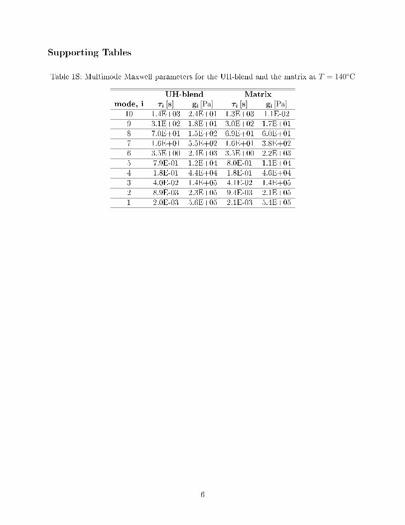
Table 1S: Multimode Maxwell parameters for the UH-blend and the matrix at T = 140◦C

UH-blend Matrix

mode, i τi [s] gi [Pa] τi [s] gi [Pa]10 1.4E+03 2.4E+01 1.3E+03 1.1E-029 3.1E+02 1.8E+01 3.0E+02 1.7E+018 7.0E+01 1.5E+02 6.9E+01 6.0E+017 1.6E+01 5.5E+02 1.6E+01 3.8E+026 3.5E+00 2.4E+03 3.5E+00 2.2E+035 7.9E-01 1.2E+04 8.0E-01 1.1E+044 1.8E-01 4.4E+04 1.8E-01 4.6E+043 4.0E-02 1.4E+05 4.1E-02 1.4E+052 8.9E-03 2.3E+05 9.4E-03 2.1E+051 2.0E-03 5.6E+05 2.1E-03 5.4E+05

6

Supporting Figures

(a)

0 π/2 π 3π/2 2πβ

0

1

2

3

4

5

6

7

I

×10-3

Iraw

Ifit

IKebab

Ishish

(b)

0 π/2 π 3π/2 2πβ

0

1

2

3

4

5

6

7

I

×10-3

Iraw

Iβ

(c)

Figure 1S: Illutration of how scattering intensities from kebabs are extracted from SAXS-patterns while omitting the contribution from shish. (a) Example of the raw SAXS pattern.The shaded area indicate the area over which the azimuthal integration is performed. Withthe arrow showing the direction of the azimuthal angle β. (b) Azimuthal intensity pro�lewhere (black ·) is the raw data, (green −) is the total �t using Eq. (4) with (red −−) and(blue ·−) signifying the scattering contribution from kebabs and shish, respectively, withp = −1. (c) Compares the raw azimuthal intensity pro�le (black ·) and the pro�le where theshish-contribution has been removed (blue ◦) by subtracting the �tted shich contributionshown in (b).

.

7

(a) (b)

Figure 2S: Uniaxial extensional data for the UH-blend at 140◦C (a) Shows the raw data (grayscale symbols) and the averaged data (blue scale symbols) (b) Shows the reproducibility ofthe stretches for two sets of stretch experiments (blue and black symbols, respectively)

(a) (b)

Figure 3S: Parameter Sensitivity for the HMMSF modelling (lines) of constant rate exten-sional data (symbols) at 140◦C. (a) Compares the HMMSF prediction using the full 10mode frequency Maxwell spectrum obtained by combining SAOS and creep data with theprediction using the limited 7 mode spectrum obtained from SAOS alone. (b) Shows theHMMSF prediction using di�erent values of GD.

8

(a) (b)

Figure 4S: Rheological response in creep. (a) Creep compliance curves for the matrix ob-tained at various stresses at 150◦C. The overlap con�rms that measurements are performedin the linear regime. (b) Comparison of creep compliance curves for the UH-blend and thematrix.

Figure 5S: Dynamic shear viscosity 150◦C for the UH-blend and the matrix obtained viaSAOS (symbols) and creep (lines). Note the di�erence in zero-shear-rate viscosity at lowfrequencies

9

Figure 6S: Uniaxial extensional response for complementary experiments in creep (opensymbols) and constant rate (closed symbols) at 140◦C showing the same steady �ow behaviorfor the UH-blend (blue) and the matrix (red).

Figure 7S: Herman's orientation factor versus steady stress UH-blend (blue) and matrix(red) for �laments elongated at a constant Hencky strain rate. Black solid and dashed linesshow the apparent slope of 2/5 and the expected trend for amorphous systems, respectively.Open symbols represent Herman's orientation factor for �laments of the UH-blend obtainedfor uniaxial creep measurements, quenched at ε = 4 (green) and 5.5 (blue). Apart from theopen symbols, this �gure is identical to Figure 5 in the main manuscript.

10