Support vector regression model for BigData

systems

Alessandro Maria Rizzi

December 5, 2016

Abstract

Nowadays Big Data are becoming more and more important. Many sec-tors of our economy are now guided by data-driven decision processes. BigData and business intelligence applications are facilitated by the MapRe-duce programming model while, at infrastructural layer, cloud computingprovides flexible and cost effective solutions for allocating on demand largeclusters. In such systems, capacity allocation, which is the ability to opti-mally size minimal resources for achieve a certain level of performance, isa key challenge to enhance performance for MapReduce jobs and minimizecloud resource costs. In order to do so, one of the biggest challenge is tobuild an accurate performance model to estimate job execution time ofMapReduce systems. Previous works applied simulation based models formodeling such systems. Although this approach can accurately describethe behavior of Big Data clusters, it is too computationally expensive anddoes not scale to large system. We try to overcome these issues by applyingmachine learning techniques. More precisely we focus on Support VectorRegression (SVR) which is intrinsically more robust w.r.t other techniques,like, e.g., neural networks, and less sensitive to outliers in the training set.To better investigate these benefits, we compare SVR to linear regression.

1 Introduction

Today BigData applications are more and more critical in our society, since theycan broadly improve efficiency of enterprises and the quality of our lives. Forexample, according to a recent McKinsey analysis [1], BigData could have apotential impact of $300 billion to US health care only. The core of most ofthe BigData applications implemented today is constituted by the MapReduceprogramming model, which is the most common adopted solution [2]. Its opensource implementation, Hadoop, can handle very large datasets [3]; accordingto IDC [4], in 2015 Hadoop processed half of the world data. In addition, dueto a number of performance enhancements (e.g., SSD support, caching, I/Obarriers elimination) implemented in Hadoop 2.x, MapReduce can fully supportboth interactive data analysis and traditional batch applications. Further im-provements have been introduced with the Apache Tez framework, in which job

1

arX

iv:1

612.

0145

8v1

[cs

.DC

] 5

Dec

201

6

tasks are not forced to follow a strict two-phase order, but tasks can form anarbitrary complex directed-acyclic-graph and I/O barriers are totally eliminatedfrom intermediate computations.

In this scenario, however, a challenging problem is to estimate the perfor-mance of an Hadoop (i.e., MR and Tez) job execution, i.e., predict the executiontime required for completing a job. Performance prediction of BigData appli-cations is extremely important, e.g., for correctly planning the required size acluster (either physical or in the public cloud) must have to handle a certainworkload. Traditionally, the only reliable way to predict performance has beento conduct a costly and time-consuming empirical evaluation [5]. To overcomethese disadvantages, different models for performance prediction have been de-veloped. However, modeling BigData performance is becoming more and moredifficult: if we consider the recent improvements introduced by Hadoop 2.x indynamically handling containers between map and reduce tasks or Tez DAGnodes, along with improving the overall cluster utilization, they also increasedthe model complexity. If we look, then, to computational paradigms newerthan MapReduce, e.g., Apache Tez, modeling performance become extremelychallenging. In fact there are in literature examples of simulation based ana-lytic models (TODO REF); however, due to the number of intermediate layersinvolved, are extremely computationally demanding.

In this work we address the problem of performance prediction through theuse of machine learning techniques. The idea is that instead of manually builda model which relates a job execution time to some of its features, machinelearning techniques extract from a set of experiments this relation, which canthen be used on different jobs given their features. Namely we used linearregression and Support Vector Regression (SVR) as machine learning techniques.We compared the different techniques and found that SVR performed better,since linear regression was not always applicable; nonetheless in few cases linearregression provided better results.

The rest of the paper is structured as follows: in Section 2 we briefly describethe machine learning techniques involved and the framework Hadoop and Tez.In Section 3 we explain the goals of this work and how we selected the relevantmachine learning techniques features. In Section 4 we provide a description of theexperiments we made for validating the approach and their results. Section 5introduces the relevant related works. Finally, in Section 6 we draw someconclusions and present some possible future research directions.

2 Background

In this section we introduce the main machine learning approach used in thiswork and the Apache Hadoop and Tez frameworks.

2

2.1 Linear regression

Linear regression is a common statistical tool for finding a linear relation betweenan observed variable and a (set of) explanatory variables.

Given a set of m training points {(x1, y1), . . . , (xm, ym)} where xi ∈ Rn,yi ∈ R are the feature vector and the target output respectively; the purpose oflinear regression is to find the linear function f(x) : Rn → R which minimizesthe least-square error, i.e.,

∑mi=1(yi− f(xi))

2. Given that f(x) is linear we have:f(x) = wT x+ b,w ∈ Rn, thus obtaining the following optimization problem:

minw,b

m∑

i=1

(yi − wT xi − b)2

with w ∈ Rn, b ∈ R

There is a huge amount of literature on linear regression, including severalways for efficiently computing it. Refer to specific literature, e.g., [6], for furtherdetails.

2.2 Support Vector Regression

Support Vector Regression (SVR) is a popular machine learning approach firstdescribed by V. Vapnik [7], famous for its robustness and insensitivity on outliers.In addition, it can scale to several dimensions.

This section is divided as follows: in Section 2.2.1 we define the basic SVRapproach; in Section 2.2.2 we describe an SVR extension to handle non-linearmodels.

2.2.1 Formulation

Given a set of m training points {(x1, y1), . . . , (xm, ym)} where xi ∈ Rn, yi ∈ Rare the feature vector and the target output respectively; the purpose of SVR isto find the “flattest” linear function f(x) : Rn → R which approximates everypoint in the training set with an error lower that ε, i.e., ∀i ∈ [1,m].|yi−f(xi)| < ε.Since f(x) is linear, f(x) = wT x+ b, thus the flatness of f(x) depends on vectorw ∈ Rn being small. So we can search f(x) as the linear function having thesmallest norm of w, satisfying the constraint on the maximum error ε. We obtainthe following optimization problem:

minw,b

1

2wT w

subject to

{yi − wT xi − b ≤ εwT xi + b− yi ≤ ε

with w ∈ Rn, b ∈ R

3

Since function f(x) could not exists if ε is too small, we can relax ourconstraint over ε. We obtain the following problem:

minw,b,ξ,ξ∗

1

2wT w + C

m∑

i=1

(ξi + ξ∗i )

subject to

yi − wT xi − b ≤ ε+ ξiwT xi + b− yi ≤ ε+ ξ∗iξi, ξ

∗i ≤ 0

with w ∈ Rn, b ∈ R

In practice we add the slack variables ξi, ξ∗i to relax the constraint on the

maximum allowed error. It is possible to tune error sensitivity through parameterC: the smaller is C the more errors are ignored; on the contrary the bigger isC the more the deviations from the points above ε are considered. Althoughthis formulation better describe SVR foundations, SVR is usually solved byconsidering the dual problem and reducing to a quadratic programming problem(see, e.g., [8]).

2.2.2 Kernels

It is also possible to make the SVR non-linear, which is applicable in case thetarget output has a non-linear dependency on the feature vector, on which thetraditional SVR would perform poorly. The basic idea is to preprocess thefeature vector through a map φ : Rn → Rl. The optimization problem thusbecomes:

minw,b,ξ,ξ∗

1

2wT w + C

m∑

i=1

(ξi + ξ∗i )

subject to

yi − wTφ(xi)− b ≤ ε+ ξiwTφ(xi) + b− yi ≤ ε+ ξ∗iξi, ξ

∗i ≤ 0

with w ∈ Rn, b ∈ R

In such way it is possible to obtain a non-linear function f(x). Note that thefunction mapping φ is usually not explicitly given, since it quickly becomes un-feasible for the large number of features.Instead it is implicitly specified throughfunction K(xi, xj) which computes the dot product between the given vectors,i.e., K(xi, xj) = φ(xi)

Tφ(xj). We provide in Table 1 the kernel functions whichwere used in our experiments. We point the reader to [8] for further details onSVR.

4

Table 1: Kernel functions

Kernel Kernel function

Linear K(xi, xj) = xTi xj (1)

Polynomial with degree d K(xi, xj) = (xTi xj

n )d (2)

Gaussian K(xi, xj) = e−(xi−xj)T (xi−xj)

n (3)

2.3 MapReduce

MapReduce is a general computational paradigm, firstly implemented by Googlein [9]. Hadoop is an open-source implementation of MapReduce. MapReducesplits the job execution into two main phases: map and reduce. The goal ofMapReduce is to be able to scale to huge dataset, in a fault-tolerant way: forthese reasons a MapReduce job is executed in a cluster and both phases are splitinto a number of tasks executed on different nodes. An additional shuffle phaseis thus added after the map phase, in order to provide map intermediate resultsto reduce tasks and eventually relocate the computation data among differentnodes.

During the map phase input data is partitioned, with every map task pro-cessing a partition. In fact the number of map tasks depends on input data size.The result of a map task is a set of key-value pairs which is further processedduring the rest of the job. During the shuffle phase the output of the map issorted to the node executing the reduce tasks according to the value of the key.Every key is fetched by only one reduce task. The reduce phase would take careof finalizing the computation on the key-value pairs received. Typically eachreduce task would aggregate the key-value pairs received into a summary.

2.4 Hadoop YARN

Hadoop is the open source implementation of the MapReduce paradigm. HadoopYet Another Resource Negotiator (YARN) is the core of the second version ofHadoop, which completely changes Hadoop architecture, being also able toaccommodate other paradigms than MapReduce.

The purpose of YARN is to manage the resource of the cluster among thedifferent applications: instead of dedicated map and reduce slots which charac-terized the first version of Hadoop, resources are organized in containers whichdefine a minimal unit of CPU and memory resources.

The assignment of containers to applications is done by the Resource Man-ager (RM), a process executed on the master node which assigns the resourcesaccording to a given scheduler, defining the optimal policy. The standard sched-uler are Capacity scheduler and Fair scheduler. Capacity scheduler statically

5

Pig/Hive-MR versus Pig/Hive-Tez

© Hortonworks Inc. 2013

Pig/Hive-MR versus Pig/Hive-Tez SELECT a.state, COUNT(*), AVERAGE(c.price)

FROM a JOIN b ON (a.id = b.id)

JOIN c ON (a.itemId = c.itemId) GROUP BY a.state

Pig/Hive - MR Pig/Hive - Tez

I/O Synchronization Barrier

I/O Synchronization Barrier

Job 1

Job 2

Job 3

Single Job

Danilo Ardagna - MapReduce and Hadoop Ecosystem 264

Figure 1: MR and Tez execution of a Pig/Hive query

divide the cluster resources among the different organizations accessing the clus-ter. Fair scheduler, instead, aims to assign an equal amount of resources todifferent applications. In our experiments we always used Capacity scheduler.

To monitor each single application an instance of the Application Mas-ter (AM) is created per node. AM monitors the application state and caninteract with the RM to ask more resources. Finally an instance of Node Man-ager (NM) is run on each node to monitor its state and notify the RM. NM alsoreceives the container requests from the different AMs.

2.5 Apache Tez

Apache Tez is a framework which works on top of Hadoop YARN to providea new computational paradigm. Traditional MapReduce requires the job to bestructured in a phase of map task followed by a phase of reduce task. To meet thisrequirement, complex applications, e.g., some Hive queries, have to be split intoseveral MapReduce jobs. Tez allows jobs constituted by an arbitrary complexdirected acyclic graphs (DAGs) of map, reduce and reduce/reduce stages, whichcan be solved more efficiently than the translation into pure MapReduce jobsreducing I/O barriers (see, e.g., Figure 1).

3 Research goals

The objective of this research is to apply machine learning techniques to predictthe performance of BigData job execution, in our case single MapReduce jobs andTez jobs constituted by a DAG of tasks. The overall idea is that job executiontime depends on a complex relation among some features describing the job and

6

the cluster. We plan to obtain an approximation of such relation using machinelearning techniques as linear regression and SVR over a set of job executionsand use it to predict the execution time obtained by changing the conditionswith respect to the training environment, i.e., changing the job or the clusterconfiguration.

First of all we want, on the basis of the relation obtained through the machinelearning techniques, predict the performance of a cluster with a different numberof CPU cores than the one used for training. Then we would like to use themodel trained on one job to predict the execution time of a different job orthe same job over a different dataset. Of course, the necessary condition toobtain good results is to choose suitable features, which can characterize thepair job-cluster. In the rest of this section we describe the features we selectedalong with the motivations such choice.

3.1 Feature selection

In this section we describe the features used to predict the job duration. Webased our choice of features on the basis of previous works as [10] and [11].In these works it is used a model for MapReduce job execution time based onthe number of map and reduce tasks of the job, the average and maximumduration of map, shuffle and reduce tasks and the available number of CPUcores. We considered all these features, analyzing different choices for expressingthe number of CPU cores. The reason is that in the models of [10] and [11]the execution time is inversely proportional with respect to the number of CPUcores. This is, of course, reasonable: the more computational resources areadded, the more the execution time should be reduced. However, the machinelearning techniques can find only linear models in the feature set, and inverseproportionality can be handled, e.g., by introducing non-linear feature. Wethen analyzed different candidate features for the number of CPU cores, whichwere considered one at a time along with the other features. These candidateshave been: the plain number of CPU cores (numCores), the reciprocal of thenumber of cores ( 1

numCores ), and a combination of the number of CPU coreswith the number of map numMap and reduce tasks numReduce (terms includedwithin [10] approximated formula), numMap

numCores and numReducenumCores .

In addition to these features justified by models presented in literature, wealso considered other ones. In particular we introduced some measures of theamount of data involved in the job: a descriptor of the data size involved in thejob and the average and maximum number of bytes transferred during shuffles.

All the features we have discussed so far have been used for pure two stageMapReduce jobs. For what concerns Tez jobs, we considered the same featureswe discussed up to now, considering the map, shuffle and reduce average andmaximum time of the task for each stage of the job DAG. This choice in factsimply generalize the approach taken for MapReduce jobs, however, it does notallow to generalize the trained model to jobs with different DAGs.

7

select avg ( ws quant i ty ) ,avg ( w s e x t s a l e s p r i c e ) ,avg ( w s e x t w h o l e s a l e c o s t ) ,sum( w s e x t w h o l e s a l e c o s t )from web sa l e swhere ( web sa l e s .

w s s a l e s p r i c ebetween 100.00 and 150 .00)or ( web sa l e s . w s n e t p r o f i tbetween 100 and 200)group by ws web page skl imit 100 ;

(a) R1

select i nv i t em sk ,inv warehouse sk

from inventorywhere inv quant i ty on hand >

10group by i nv i t em sk ,

inv warehouse skhaving sum(

inv quant i ty on hand ) > 20l imit 100 ;

(b) R2

select avg ( s s q u a n t i t y ) ,avg ( s s n e t p r o f i t )from s t o r e s a l e swhere s s q u a n t i t y > 10and s s n e t p r o f i t > 0group by s s s t o r e s khaving avg ( s s q u a n t i t y ) > 20l imit 100 ;

(c) R3

select c s i t em sk , avg (c s quan t i t y ) as aq

from c a t a l o g s a l e swhere c s quan t i t y > 2group by c s i t e m s k ;

(d) R4

select inv warehouse sk ,sum( inv quant i ty on hand )from inventorygroup by inv warehouse skhaving sum(

inv quant i ty on hand ) > 5l imit 100 ;

(e) R5

Figure 2: MapReduce Hive queries

3.2 Machine learning techniques selection

We apply the learning of BigData jobs execution time dependency from the pre-viously mentioned features using different approaches, involving linear regressionand SVR. We used linear regressing as a baseline; we applied SVR both withand without kernels (Equation 1, see Table 1). The kernels we considered arethe polynomial (Equation 2) with degree 2,3,4,6 and Gaussian (Equation 3).

4 Experimental evaluation

We now analyze and compare linear regression and SVR. The section is organizedas follows: in Section 4.1 we describe the benchmark used and the clusters onwhich the benchmark has been executed. In Section 4.2, instead, we present andanalyze the obtained results.

8

select a . aq from ( select c s i t em sk , avg ( c s quan t i t y ) as aqfrom c a t a l o g s a l e swhere c s quan t i t y > 2group by c s i t e m s k ) a join ( select i i t em sk , i c u r r e n t p r i c e

from itemwhere i c u r r e n t p r i c e > 2order by i c u r r e n t p r i c e )b on a . c s i t e m s k = b . i i t e m s k

order by a . aql imit 100 ;

(a) Q2

select avg ( ws quant i ty ),avg ( w s e x t s a l e s p r i c e ),avg ( w s e x t w h o l e s a l e c o s t ),sum( w s e x t w h o l e s a l e c o s t )from web sa l e swhere ( web sa l e s .

w s s a l e s p r i c e between100.00 and 150 .00) or (web sa l e s . w s n e t p r o f i tbetween 100 and 200)

l imit 100 ;

(b) Q3

select i nv i t em sk ,inv warehouse sk

from inventory whereinv quant i ty on hand > 10

group by i nv i t em sk ,inv warehouse sk

having sum(inv quant i ty on hand )>20

order by inv warehouse skl imit 100 ;

(c) Q4

Figure 3: Tez Hive queries

4.1 Experimental setup

We considered as a benchmark different Hive queries applied on the TPC-DS1

dataset. TPC-DS ha been chosen since it is the reference benchmark for datawarehousing. We used queries R1-5, shown in Figure 2, as MapReduce jobs; andqueries Q2-4, shown in Figure 3, as Apache Tez jobs. We applied them ontodifferent datasets ranging from 250GB to 1TB for R1-5 and ranging from 40GBto 50GB for Q2-4.

All our MapReduce experiments were run on CINECA, the Italian super-computing center, on the Big Data cluster PICO2. The experiments involvingApache Tez were instead performed on a dedicated cluster on Flexiant3.

4.1.1 PICO cluster

PICO is composed of 74 nodes, each of them having two Intel Xeon 10 Core2670 v2@2.5GHz, and 128GB of memory per node. Of this 74 nodes, up to 66are available for computation. In our experiments on PICO, we used severalconfigurations ranging from 40 to 120 cores and set up the scheduler to provideone container per core.

1http://www.tpc.org/tpcds/2http://www.hpc.cineca.it/hardware/pico3https://www.flexiant.com/

9

The cluster is shared among different users, it provides the Portable BatchSystem (PBS) PBS Professional to submit jobs and check their execution: it ispossible to schedule a given job for execution on a given number of nodes usingeach a certain number of CPU cores and memory. Since the cluster is sharedamong different users, the performance of the execution of the single job dependson the general load of the system, even though the PBS try to split the resourcesamong the different users. This especially affects the storage performance, sinceit is not handled directly by the PBS and for a large part of it is separated fromthe local computation nodes. Due to this, it is possible to have large variationsin the performance of the class, according to the total usage of the cluster.

We tried to mitigate this variability first of all by requesting entire nodes ofthe cluster for the execution of our experiments. In such way, we could reasonablybe sure that nobody else could run other jobs on those nodes and thus interferingto the performance measurement. Every experiment is run into an ephemeralHadoop cluster built into the selected node, which is created at the beginning ofthe experiment. The PICO cluster provides the myHadoop tool for setting up anHadoop 2.5.1 cluster, upon which we used Hive version 1.2.1. The HDFS storageis kept locally on the selected node, which diminishes the amount of variabilitywith respect to the centralized storage. In spite of these precautions, still theexperiment shown high variability, in particular with few runs characterized byextremely high execution time. To further reduce this, we discarded from ouranalysis experimental runs which behave significantly different. The criteria weused consist in discarding all the experiments with a difference from the averagelarger than 3 times the standard deviation.

4.1.2 Cluster Flexiant

The cluster Flexiant is part of an IaaS public cloud. It is composed of 7 nodes,of which 2 are master nodes and 5 slave (computational) nodes. Each node has4 CPU cores and 8GB of memory. The cluster is provided with HortonworksData Platform (HDP) 2.3, which includes Hadoop 2.7.1 and Hive 1.2.1. Againwe kept the HDFS storage local to each node to reduce variability.

4.2 Experimental result

In this section we describe the experiments we conducted to assess the accuracyof machine learning approaches to predict job duration.

The purpose of this section is to assess the performance of machine learningtechniques to predict BigData job execution time. First we check that the featurewe defined are adequate by predicting the execution of jobs equals to the onesused for training. Then we check how the machine learning techniques canpredict the execution time for a different number of CPU cores or a differentquery.

Each experiment has been conducted in the following way: the relevant datahas been partitioned in three parts: a training set, a cross-validation set anda testing set. The machine learning approach is trained on the training set.

10

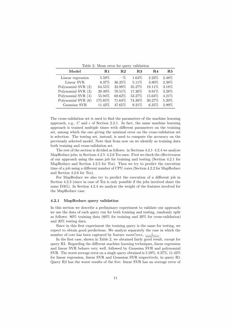
Table 2: Mean error for query validation

Model R1 R2 R3 R4 R5

Linear regression 5.59% —% 1.64% 2.23% 2.48%Linear SVR 8.37% 36.25% 5.11% 3.80% 2.38%

Polynomial SVR (2) 64.55% 32.98% 35.27% 19.11% 3.18%Polynomial SVR (3) 20.49% 70.51% 17.26% 9.91% 3.28%Polynomial SVR (4) 55.94% 68.62% 53.27% 15.63% 4.21%Polynomial SVR (6) 175.85% 71.64% 74.38% 30.27% 5.20%

Gaussian SVR 11.43% 47.65% 9.21% 6.35% 2.99%

The cross-validation set is used to find the parameters of the machine learningapproach, e.g., C and ε of Section 2.2.1. In fact, the same machine learningapproach is trained multiple times with different parameters on the trainingset, among which the one giving the minimal error on the cross-validation setis selection. The testing set, instead, is used to compute the accuracy on thepreviously selected model. Note that from now on we identify as training databoth training and cross-validation set.

The rest of the section is divided as follows: in Sections 4.2.1–4.2.4 we analyzeMapReduce jobs; in Sections 4.2.5–4.2.6 Tez ones. First we check the effectivenessof our approach using the same job for training and testing (Section 4.2.1 forMapReduce and Section 4.2.5 for Tez). Then we try to predict the executiontime of a job using a different number of CPU cores (Section 4.2.2 for MapReduceand Section 4.2.6 for Tez).

For MapReduce we also try to predict the execution of a different job inSection 4.2.3 (since in case of Tez is only possible if the jobs involved share thesame DAG). In Section 4.2.4 we analyze the weight of the features involved forthe MapReduce case.

4.2.1 MapReduce query validation

In this section we describe a preliminary experiment to validate our approach:we use the data of each query run for both training and testing, randomly splitas follows: 80% training data (60% for training and 20% for cross-validation)and 20% testing data.

Since in this first experiment the training query is the same for testing, weexpect to obtain good predictions. We analyze separately the case in which thenumber of core has been captured by feature numCores, 1

numCores .In the first case, shown in Table 2, we obtained fairly good result, except for

query R2. Regarding the different machine learning techniques, linear regressionand linear SVR behave very well, followed by Gaussian SVR and polynomialSVR. The worst average error on a single query obtained is 5.59%, 8.37%, 11.43%for linear regression, linear SVR and Gaussian SVR respectively, in query R1.Query R2 has the worst results of the five: linear SVR has an average error of

11

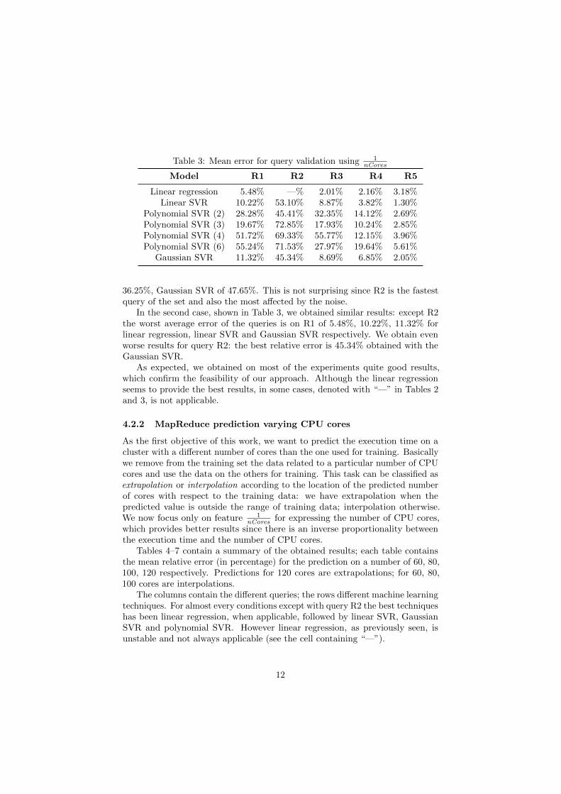
Table 3: Mean error for query validation using 1nCores

Model R1 R2 R3 R4 R5

Linear regression 5.48% —% 2.01% 2.16% 3.18%Linear SVR 10.22% 53.10% 8.87% 3.82% 1.30%

Polynomial SVR (2) 28.28% 45.41% 32.35% 14.12% 2.69%Polynomial SVR (3) 19.67% 72.85% 17.93% 10.24% 2.85%Polynomial SVR (4) 51.72% 69.33% 55.77% 12.15% 3.96%Polynomial SVR (6) 55.24% 71.53% 27.97% 19.64% 5.61%

Gaussian SVR 11.32% 45.34% 8.69% 6.85% 2.05%

36.25%, Gaussian SVR of 47.65%. This is not surprising since R2 is the fastestquery of the set and also the most affected by the noise.

In the second case, shown in Table 3, we obtained similar results: except R2the worst average error of the queries is on R1 of 5.48%, 10.22%, 11.32% forlinear regression, linear SVR and Gaussian SVR respectively. We obtain evenworse results for query R2: the best relative error is 45.34% obtained with theGaussian SVR.

As expected, we obtained on most of the experiments quite good results,which confirm the feasibility of our approach. Although the linear regressionseems to provide the best results, in some cases, denoted with “—” in Tables 2and 3, is not applicable.

4.2.2 MapReduce prediction varying CPU cores

As the first objective of this work, we want to predict the execution time on acluster with a different number of cores than the one used for training. Basicallywe remove from the training set the data related to a particular number of CPUcores and use the data on the others for training. This task can be classified asextrapolation or interpolation according to the location of the predicted numberof cores with respect to the training data: we have extrapolation when thepredicted value is outside the range of training data; interpolation otherwise.We now focus only on feature 1

nCores for expressing the number of CPU cores,which provides better results since there is an inverse proportionality betweenthe execution time and the number of CPU cores.

Tables 4–7 contain a summary of the obtained results; each table containsthe mean relative error (in percentage) for the prediction on a number of 60, 80,100, 120 respectively. Predictions for 120 cores are extrapolations; for 60, 80,100 cores are interpolations.

The columns contain the different queries; the rows different machine learningtechniques. For almost every conditions except with query R2 the best techniqueshas been linear regression, when applicable, followed by linear SVR, GaussianSVR and polynomial SVR. However linear regression, as previously seen, isunstable and not always applicable (see the cell containing “—”).

12

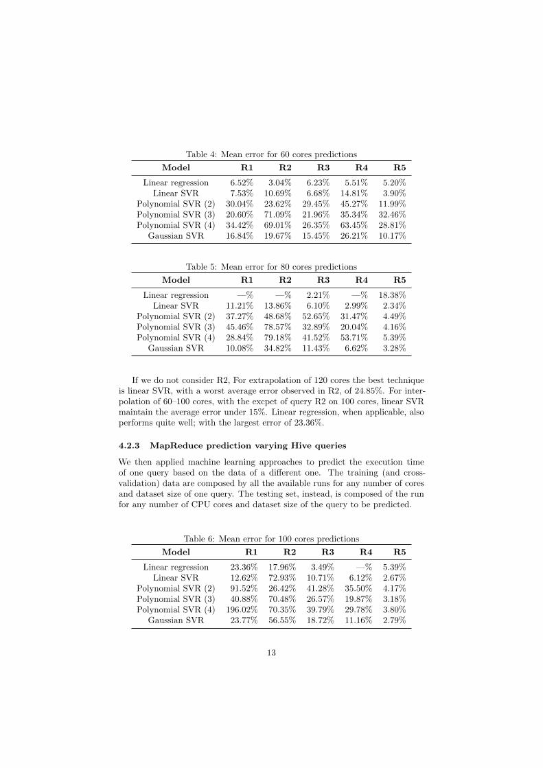
Table 4: Mean error for 60 cores predictions

Model R1 R2 R3 R4 R5

Linear regression 6.52% 3.04% 6.23% 5.51% 5.20%Linear SVR 7.53% 10.69% 6.68% 14.81% 3.90%

Polynomial SVR (2) 30.04% 23.62% 29.45% 45.27% 11.99%Polynomial SVR (3) 20.60% 71.09% 21.96% 35.34% 32.46%Polynomial SVR (4) 34.42% 69.01% 26.35% 63.45% 28.81%

Gaussian SVR 16.84% 19.67% 15.45% 26.21% 10.17%

Table 5: Mean error for 80 cores predictions

Model R1 R2 R3 R4 R5

Linear regression —% —% 2.21% —% 18.38%Linear SVR 11.21% 13.86% 6.10% 2.99% 2.34%

Polynomial SVR (2) 37.27% 48.68% 52.65% 31.47% 4.49%Polynomial SVR (3) 45.46% 78.57% 32.89% 20.04% 4.16%Polynomial SVR (4) 28.84% 79.18% 41.52% 53.71% 5.39%

Gaussian SVR 10.08% 34.82% 11.43% 6.62% 3.28%

If we do not consider R2, For extrapolation of 120 cores the best techniqueis linear SVR, with a worst average error observed in R2, of 24.85%. For inter-polation of 60–100 cores, with the excpet of query R2 on 100 cores, linear SVRmaintain the average error under 15%. Linear regression, when applicable, alsoperforms quite well; with the largest error of 23.36%.

4.2.3 MapReduce prediction varying Hive queries

We then applied machine learning approaches to predict the execution timeof one query based on the data of a different one. The training (and cross-validation) data are composed by all the available runs for any number of coresand dataset size of one query. The testing set, instead, is composed of the runfor any number of CPU cores and dataset size of the query to be predicted.

Table 6: Mean error for 100 cores predictions

Model R1 R2 R3 R4 R5

Linear regression 23.36% 17.96% 3.49% —% 5.39%Linear SVR 12.62% 72.93% 10.71% 6.12% 2.67%

Polynomial SVR (2) 91.52% 26.42% 41.28% 35.50% 4.17%Polynomial SVR (3) 40.88% 70.48% 26.57% 19.87% 3.18%Polynomial SVR (4) 196.02% 70.35% 39.79% 29.78% 3.80%

Gaussian SVR 23.77% 56.55% 18.72% 11.16% 2.79%

13

Table 7: Mean error for 120 cores predictions

Model R1 R2 R3 R4 R5

Linear regression 49.67% 2.89% 10.00% 11.83% 34.09%Linear SVR 8.93% 24.85% 22.33% 8.03% 2.83%

Polynomial SVR (2) 61.33% 53.23% 65.48% 78.85% 5.37%Polynomial SVR (3) 123.09% 73.79% 55.10% 48.98% 4.35%Polynomial SVR (4) 113.89% 70.42% 59.48% 103.42% 4.47%

Gaussian SVR 50.46% 107.83% 56.34% 30.66% 3.03%

Table 8: Mean error for query-query prediction with nCores

Model R5→R2 R2→R5 R3→R4 R4→R3

Linear regression 7.67% 42.11% 8.87% 10.39%Linear SVR 46.76% 278.68% 18.31% 10.71%

Polynomial SVR (2) 46.76% 390.74% 139.63% 60.33%Polynomial SVR (3) 46.76% 319.74% 126.14% 46.56%

Gaussian SVR 46.76% 2781.36% 52.76% 27.27%

In this case we focus on numCores results, which are shown in Tables 8 and 9.Tables 10 and 11, intead, show the results for 1

numCores .First we use for training and test similar queries. We start by predicting R2

from R5 and vice-versa. In both case, we obtain mixed result; the techniqueproviding best results is linear regression, followed by linear SVR, GaussianSVR and polynomial SVR. For linear regression we have an error of 7.67% forpredicting R2 from R5, and 42.11% when predicting R5 from R2. This is notvery surprising since these queries, especially R2, are characterized by smallexecution time and high noise, as we have previously seen. If we consider R3and R4, we obtain much better results: an error of 8.87%, 18.31% for linearregression and linear SVR respectively when predicting R4 from R3; an errorof 10.39%,10.71% respectively the other way around. Again the order of themachine leaning techniques performance is the same, with linear regression andlinear SVR dominating and polynomial SVR at the end.

In both previous cases we trained and tested either two fast queries or twoslow ones. Now, we validate the case in which we train on a combination offast-slow queries and test an intermediate one. In practice we predict R3 on thetraining over R1,R2, and R4. The results are pretty good: the average error is5.64% and 6.12% for linear regression and linear SVR respectively; again therank of performances among the machine learning techniques is the same.

The last evaluation we attempted has been to mix different queries, which ispredict R3 from R2 and R5 and predict R2 from R3 and R4. In this case theresult were pretty bad, in a way remarking the fact that the queries consideredare too different to be generalized.

14

Table 9: Mean error for multiquery-query prediction with nCores

Model R1,R2,R4→R3 R2,R5→R3 R3,R4→R2

Linear regression 5.64% 86.89% 154.94%Linear SVR 6.12% 73.15% 68.54%

Polynomial SVR (2) 46.12% 81.33% 1784.38%Polynomial SVR (3) 36.92% 80.25% 1111.44%

Gaussian SVR 11.92% 59.76% 811.19%

Table 10: Mean error for query-query prediction with 1nCores

Model R5→R2 R2→R5 R3→R4 R4→R3

Linear regression 8.30% 43.30% 8.66% 11.33%Linear SVR 46.76% 343.38% 16.45% 12.59%

Polynomial SVR (2) 46.76% 430.90% 95.42% 65.41%Polynomial SVR (3) 46.76% 323.27% 170.83% 36.24%

Gaussian SVR 46.76% 2741.39% 51.27% 24.87%

4.2.4 MapReduce weight of the selected features

In this section we analyze the importance each of the selected features has inthe prediction of the query execution time. We can see that analyzing theweight each feature has in the execution time estimation. Table 12 shows theweights considering for the cluster size either numCore or 1

numCore for all theR1-5 queries. If we analyze all the features, considering the number of core asfeature numCore, the dominant feature is the max shuffle time, which has aweight of 0.9355. Then, there are the average number of bytes transferred, witha weight of 0.1972; the average time of a reduce task, weight 0.1413. All theother features have weights less than 0.06.

If we switch feature numCore with its inverse 1numCore , we obtain similar

results: again the feature with highest weight is the maximum shuffle task time(0.9327), followed by the average number of bytes transferred and the averagetime of a reduce task, with weights -0.1550 and 0.1376 respectively.

Table 11: Mean error for multiquery-query prediction with 1nCores

Model R1,R2,R4→R3 R2,R5→R3 R3,R4→R2

Linear regression 5.84% 87.05% 190.06%Linear SVR 6.10% 73.44% 97.69%

Polynomial SVR (2) 44.96% 81.40% 1670.06%Polynomial SVR (3) 33.68% 80.25% 1275.93%

Gaussian SVR 12.61% 62.68% 826.95%

15

Table 12: Feature weight

Feature nCores 1nCores

Map tasks 0.029655 0.059395Reduce tasks −0.025907 −0.053398

Average map task duration 0.022160 0.029537Maximum map task duration 0.013312 0.009639Average reduce task duration 0.141263 0.137604

Maximum reduce task duration 0.002008 0.008253Average shuffle task duration −0.025151 −0.025066

Maximum shuffle task duration 0.935545 0.932685Average bytes transferred per shuffle task −0.197170 −0.154967

Maximum bytes transferred per shuffle task 0.056686 0.007358Dataset size 0.015942 0.012835

Number of CPU cores −0.024642 0.020706

Table 13: Mean error for query validation

Model Q2 Q3 Q4

Linear regression 1.71% 2.67% 4.90%Linear SVR 1.63% 5.77% 4.15%

Polynomial SVR (2) 11.52% 19.05% 16.63%Polynomial SVR (3) 5.14% 7.83% 7.02%Polynomial SVR (4) 11.39% 14.70% 12.80%Polynomial SVR (6) 11.58% 14.65% 14.98%

Gaussian SVR 2.56% 3.00% 3.80%

By analyzing the weights for each query individually, we note that the max-imum shuffle task time has an high weight especially for long queries, e.g., R1(0.8306) and R3 (0.9866). The fast queries (R2, R5) shows instead different be-haviors: R2 is strongly dependent on the maximum time of a map task (0.8010);R5 on average and maximum bytes transferred per shuffle task(-0.5889 and0.6072), followed by average map task time and number of map and reduce tasks(0.4805, 0.3576, 0.4186).

4.2.5 Tez query validation

In this section we show the result of the same validation described in Section 4.2.1to Tez queries Q2-4. Again we use the data of each query run for both trainingand testing: 80% training data (60% for training and 20% for cross-validation)and 20% testing data. We focused on the 50GB dataset for every query Q2, Q3and Q4.

The results are shown in Tables 13 and 14. In this case the results are prettygood, the mean error is under 7% in every case with the exception of polynomial

16

Table 14: Mean error for query validation using 1nCores

Model Q2 Q3 Q4

Linear regression 2.88% 2.67% 5.98%Linear SVR 2.86% 6.85% 6.27%

Polynomial SVR (2) 9.66% 19.16% 13.27%Polynomial SVR (3) 6.71% 9.03% 7.34%Polynomial SVR (4) 9.98% 15.42% 10.81%Polynomial SVR (6) 11.43% 15.49% 11.58%

Gaussian SVR 2.94% 2.85% 4.03%

Table 15: Mean error for 8 cores predictions

Model Q2 Q3 Q4

Linear regression 19.96% —% 38.24%Linear SVR 14.58% 26.21% 31.33%

Polynomial SVR (2) 37.95% 69.80% 60.60%Polynomial SVR (3) 13.41% 70.69% 10.92%

Gaussian SVR 13.71% 9.09% 14.71%

SVR for both nCores and 1nCores . The best machine learning techniques are linear

SVR, Gaussian SVR and linear regression which have comparable performance,followed by polynomial SVR.

4.2.6 Tez prediction varying CPU cores

We now repeat for Tez queries the analysis shown in Section 4.2.2 for MapReducequeries. In this case we try to use the data gathered from all the cluster sizeexcept one for training and then use the learned model to predict the executiontime of the missing size. In this case, we applied this procedure for cores 8,12, 16 and 20. As before, 8 and 20 cores predictions are cases of extrapolation,since the size is outside the range of the available dataset; 12 and 16, instead,are cases of interpolation. We thus expect better results for 12 and 16 cores,with respect to 8 and 20. We show here, in Tables 15–18, the obtained resultsusing 1

nCores . We obtained the best results for 12 cores, in which the meanerror of linear regression, linear SVR and Gaussian SVR is always lower than17%. For 16 cores, only Gaussian SVR produce acceptable results, with meanerror less than 21% for every condition. The case with 20 cores gives the worstresult; Gaussian SVR produce has mean error less than 43% for every condition.Finally for 8 cores, again the Gaussian SVR yields the best result, with a meanerror under 15% in every case.

17

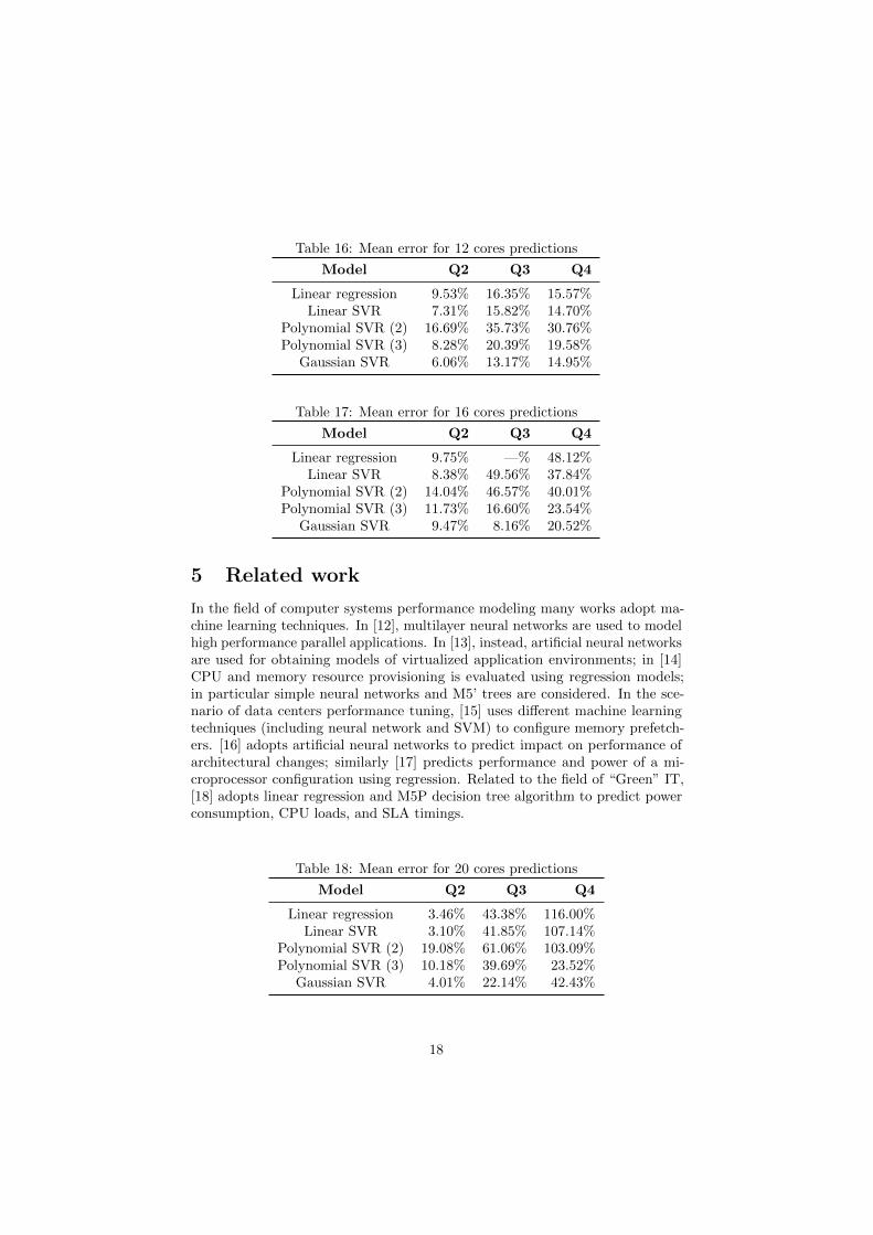
Table 16: Mean error for 12 cores predictions

Model Q2 Q3 Q4

Linear regression 9.53% 16.35% 15.57%Linear SVR 7.31% 15.82% 14.70%

Polynomial SVR (2) 16.69% 35.73% 30.76%Polynomial SVR (3) 8.28% 20.39% 19.58%

Gaussian SVR 6.06% 13.17% 14.95%

Table 17: Mean error for 16 cores predictions

Model Q2 Q3 Q4

Linear regression 9.75% —% 48.12%Linear SVR 8.38% 49.56% 37.84%

Polynomial SVR (2) 14.04% 46.57% 40.01%Polynomial SVR (3) 11.73% 16.60% 23.54%

Gaussian SVR 9.47% 8.16% 20.52%

5 Related work

In the field of computer systems performance modeling many works adopt ma-chine learning techniques. In [12], multilayer neural networks are used to modelhigh performance parallel applications. In [13], instead, artificial neural networksare used for obtaining models of virtualized application environments; in [14]CPU and memory resource provisioning is evaluated using regression models;in particular simple neural networks and M5’ trees are considered. In the sce-nario of data centers performance tuning, [15] uses different machine learningtechniques (including neural network and SVM) to configure memory prefetch-ers. [16] adopts artificial neural networks to predict impact on performance ofarchitectural changes; similarly [17] predicts performance and power of a mi-croprocessor configuration using regression. Related to the field of “Green” IT,[18] adopts linear regression and M5P decision tree algorithm to predict powerconsumption, CPU loads, and SLA timings.

Table 18: Mean error for 20 cores predictions

Model Q2 Q3 Q4

Linear regression 3.46% 43.38% 116.00%Linear SVR 3.10% 41.85% 107.14%

Polynomial SVR (2) 19.08% 61.06% 103.09%Polynomial SVR (3) 10.18% 39.69% 23.52%

Gaussian SVR 4.01% 22.14% 42.43%

18

For what concerns MapReduce applications performance modeling, one of themost explored directions consists in providing approximated formulas devisedto capture the framework internal mechanisms and job properties. For instance,[19] obtain in this way a parametric model to predict performance given thecluster configuration and application-specific data.

Building upon similar analytical models, [20] take into account the detri-mental effects of resource contention and task failures to achieve a more preciseprediction of completion times. [21], instead, explore the impact on perfor-mance of exploiting heterogeneous computational nodes in Cloud-based Hadoopclusters, allowing for tailoring resources to the needs of specific applications.

More recently, as in our work, machine learning techniques are used tosupport performance prediction of Hadoop clusters. [22] compare through anexperimental campaign several methods, ranging from ordinary linear regressionto advanced techniques as neural networks, model trees, and support vectorregression (SVR). In most experiments SVR shows the best accuracy, with onlyone case where neural networks perform better.

SVR has also been adopted also to implement automated resource allocationand configuration for Cloud-based clusters, as proposed by [23]. The describedAROMA system mines historical execution data in order to profile past sub-missions, then it robustly matches incoming jobs to the available performancesignatures for prediction. In this way, AROMA allows for meeting deadlinesstated in Service Level Agreements (SLAs) incurring minimum cost, with anaverage accuracy on completion time estimates around 12%.

Authors in [24] proposed a methodology and a framework based on multivari-ate linear regression to predict the execution time of iterative algorithms for theApache Giraph implementation able to achieve a relative prediction error around10%-30%. However, the approach is very specific to predict the performanceof DAGs analyzing homogeneous graph structures with a global convergencecondition (e.g., an accuracy threshold for the estimation of a graph metric).

With respect to previous works, we applied thoroughly different kind ofSVR, comparing the obtained results. More precisely, we applied both black-box approaches obtained through Gaussian and polynomial kernel application,to a gray box model, obtained mixing MapReduce models, which defines theinteresting features, to machine learning techniques as linear regression andSVR.

6 Conclusion and future work

The application of machine learning techniques to BigData job execution timeprediction can provide precise predictions in many situations. In particular,we obtained promising results in predicting the execution time by varying thecluster size. With respect to performance prediction of a different job, the resultsdepended of the similarity between the jobs. It is also important to remark thatsome results were biased by some noise affecting especially some queries, e.g.,R5 and R2. Overall SVR provided better results than linear regression, since in

19

different situation the latter does not converge and only in few samples providesbetter accuracy. The best results have been obtained considering the feature

1nCores , which performs better than any non-linear support vector regression(polynomial and Gaussian).

Possible future work include the application of other machine learning algo-rithm (e.g., neural networks) or the analysis on different clusters or with otherkind of BigData job (e.g., Spark4 jobs). Promising directions involve the com-bination of analytical models (e.g., queuing networks) and machine learningtechniques, e.g. reference [25]: through the use of existing expensive modelsit is possible to generate lots of data which can be fed to a machine learningtechniques to extract simpler relations, which can be further improved by addingreal data from BigData job execution in a cluster.

References

[1] J. Manyika, M. Chui, B. Brown, J. Bughin, R. Dobbs, C. Roxburgh, andA. H. Byers, Big Data: The next frontier for innovation, competition, andproductivity, McKinsey Global Institute, 2012.

[2] K.-H. Lee, Y.-J. Lee, H. Choi, Y. D. Chung, and B. Moon, “Paralleldata processing with MapReduce: A survey,” SIGMOD Rec., vol. 40,no. 4, pp. 11–20, Jan. 2012, issn: 0163-5808. doi: 10.1145/2094114.

2094118.

[3] F. Yan, L. Cherkasova, Z. Zhang, and E. Smirni, “Optimizing power andperformance trade-offs of MapReduce job processing with heterogeneousmulti-core processors,” in CLOUD, 2014. doi: 10.1109/CLOUD.2014.41.

[4] K. Kambatla, G. Kollias, V. Kumar, and A. Grama, “Trends in Big Dataanalytics,” Journal of Parallel and Distributed Computing, vol. 74, no. 7,pp. 2561–2573, 2014, issn: 0743-7315. doi: 10.1016/j.jpdc.2014.01.003.

[5] G. P. Gibilisco, M. Li, L. Zhang, and D. Ardagna, “Stage aware perfor-mance modeling of DAG based in memory analytic platforms,” in Cloud,2016.

[6] G. A. Seber and A. J. Lee, Linear regression analysis. John Wiley & Sons,2012, vol. 936.

[7] V. N. Vapnik, The nature of statistical learning theory. New York, NY,USA: Springer-Verlag New York, Inc., 1995, isbn: 0-387-94559-8.

[8] A. J. Smola and B. Scholkopf, “A tutorial on support vector regression,”Statistics and Computing, vol. 14, no. 3, pp. 199–222, 2004, issn: 1573-1375. doi: 10.1023/B:STCO.0000035301.49549.88. [Online]. Available:http://dx.doi.org/10.1023/B:STCO.0000035301.49549.88.

4https://spark.apache.org/

20

[9] J. Dean and S. Ghemawat, “MapReduce: Simplified data processing onlarge clusters,” in 6th Symposium on Operating Systems Design and Im-plementation, 2004, pp. 137–149.

[10] A. Verma, L. Cherkasova, and R. H. Campbell, “Aria: Automatic resourceinference and allocation for mapreduce environments,” in Proceedings of the8th ACM International Conference on Autonomic Computing, ser. ICAC’11, Karlsruhe, Germany: ACM, 2011, pp. 235–244, isbn: 978-1-4503-0607-2. doi: 10.1145/1998582.1998637. [Online]. Available: http:

//doi.acm.org/10.1145/1998582.1998637.

[11] M. Malekimajd, D. Ardagna, M. Ciavotta, A. M. Rizzi, and M. Passacan-tando, “Optimal map reduce job capacity allocation in cloud systems,”SIGMETRICS Perform. Eval. Rev., vol. 42, no. 4, pp. 51–61, Jun. 2015,issn: 0163-5999. doi: 10.1145/2788402.2788410. [Online]. Available:http://doi.acm.org/10.1145/2788402.2788410.

[12] E. Ipek, B. de Supinski, M. Schulz, and S. McKee, “An approach toperformance prediction for parallel applications,” English, in Euro-Par2005 Parallel Processing, ser. Lecture Notes in Computer Science, J. Cunhaand P. Medeiros, Eds., vol. 3648, Springer Berlin Heidelberg, 2005, pp. 196–205, isbn: 978-3-540-28700-1. doi: 10.1007/11549468_24. [Online].Available: http://dx.doi.org/10.1007/11549468_24.

[13] S. Kundu, R. Rangaswami, K. Dutta, and M. Zhao, “Application per-formance modeling in a virtualized environment,” in High PerformanceComputer Architecture (HPCA), 2010 IEEE 16th International Symposiumon, Jan. 2010, pp. 1–10. doi: 10.1109/HPCA.2010.5463058.

[14] J. Wildstrom, P. Stone, and E. Witchel, “Carve: A cognitive agent forresource value estimation,” in Autonomic Computing, 2008. ICAC ’08.International Conference on, Jun. 2008, pp. 182–191. doi: 10.1109/

ICAC.2008.27.

[15] S.-w. Liao, T.-H. Hung, D. Nguyen, C. Chou, C. Tu, and H. Zhou, “Ma-chine learning-based prefetch optimization for data center applications,” inHigh Performance Computing Networking, Storage and Analysis, Proceed-ings of the Conference on, Nov. 2009, pp. 1–10. doi: 10.1145/1654059.1654116.

[16] E. Ipek, S. A. McKee, R. Caruana, B. R. de Supinski, and M. Schulz,“Efficiently exploring architectural design spaces via predictive modeling,”in Proceedings of the 12th International Conference on Architectural Sup-port for Programming Languages and Operating Systems, ser. ASPLOSXII, San Jose, California, USA: ACM, 2006, pp. 195–206, isbn: 1-59593-451-0. doi: 10.1145/1168857.1168882. [Online]. Available: http:

//doi.acm.org/10.1145/1168857.1168882.

21

[17] B. C. Lee and D. M. Brooks, “Accurate and efficient regression mod-eling for microarchitectural performance and power prediction,” in Pro-ceedings of the 12th International Conference on Architectural Supportfor Programming Languages and Operating Systems, ser. ASPLOS XII,San Jose, California, USA: ACM, 2006, pp. 185–194, isbn: 1-59593-451-0. doi: 10.1145/1168857.1168881. [Online]. Available: http:

//doi.acm.org/10.1145/1168857.1168881.

[18] J. L. Berral, I. Goiri, R. Nou, F. Julia, J. Guitart, R. Gavalda, and J.Torres, “Towards energy-aware scheduling in data centers using machinelearning,” in Proceedings of the 1st International Conference on Energy-Efficient Computing and Networking, ser. e-Energy ’10, Passau, Germany:ACM, 2010, pp. 215–224, isbn: 978-1-4503-0042-1. doi: 10.1145/

1791314.1791349. [Online]. Available: http://doi.acm.org/10.1145/

1791314.1791349.

[19] X. Yang and J. Sun, “An analytical performance model of MapReduce,”in IEEE International Conference on Cloud Computing and IntelligenceSystems, (Beijing), 2011, pp. 306–310, isbn: 978-1-61284-203-5. doi:10.1109/CCIS.2011.6045080.

[20] X. Cui, X. Lin, C. Hu, R. Zhang, and C. Wang, “Modeling the performanceof MapReduce under resource contentions and task failures,” in IEEE FifthInternational Conference on Cloud Computing Technology and Science,(Bristol), 2013, pp. 158–163. doi: 10.1109/CloudCom.2013.28.

[21] Z. Zhang, L. Cherkasova, and B. T. Loo, “Performance modeling of MapRe-duce Jobs in heterogeneous Cloud environments,” in IEEE Sixth Interna-tional Conference on Cloud Computing, (Santa Clara, CA), 2013, pp. 839–846, isbn: 978-0-7695-5028-2. doi: 10.1109/CLOUD.2013.107.

[22] N. Yigitbasi, T. L. Willke, G. Liao, and D. Epema, “Towards machinelearning-based auto-tuning of MapReduce,” in IEEE 21st InternationalSymposium on Modeling, Analysis & Simulation of Computer and Telecom-munication Systems, (San Francisco, CA), 2013, pp. 11–20. doi: 10.1109/MASCOTS.2013.9.

[23] P. Lama and X. Zhou, “Aroma: Automated resource allocation and con-figuration of MapReduce environment in the Cloud,” in Proceedings ofthe 9th International Conference on Autonomic Computing, (San Jose,California, USA), ACM, 2012, pp. 63–72, isbn: 978-1-4503-1520-3. doi:10.1145/2371536.2371547.

[24] A. D. Popescu, A. Balmin, V. Ercegovac, and A. Ailamaki, “Predict:Towards predicting the runtime of large scale iterative analytics,” PVLDB,vol. 6, no. 14, pp. 1678–1689, 2013. [Online]. Available: http://www.

vldb.org/pvldb/vol6/p1678-popescu.pdf.

[25] D. Didona and P. Romano, “On bootstrapping machine learning perfor-mance predictors via analytical models,” CoRR, vol. abs/1410.5102, 2014.[Online]. Available: http://arxiv.org/abs/1410.5102.

22