Support Vector Machines

2

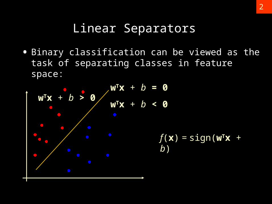
Linear Separators

• Binary classification can be viewed as the task of separating classes in feature space:

wTx + b = 0

wTx + b < 0wTx + b > 0

f(x) = sign(wTx + b)

3

Linear Separators

• Which of the linear separators is optimal?

4

Classification Margin

• Distance from example xi to the separator is

• Examples closest to the hyperplane are support vectors.

• Margin ρ of the separator is the distance between support vectors.

r

ρ

5

Maximum Margin Classification

• Maximizing the margin is good according to intuition and PAC theory.

• Implies that only support vectors matter; other training examples are ignorable.

6

Linear SVM Mathematically

• Let training set {(xi, yi)}i=1..n, xiRd, yi {-1, 1} be separated by a hyperplane. Then for each training example (xi, yi):

• For every support vector xs the distance between each xs and the hyperplane is

• Then the margin can be expressed through w and b as:

wTxi + b ≤ -1 if yi = -1wTxi + b ≥ 1 if yi = 1

w

22 r

ww

xwy 1)(

br s

Ts

yi(wTxi + b) ≥ 1

7

Linear SVMs Mathematically (cont.)

• Then we can formulate the quadratic optimization problem:

Which can be reformulated as:

Find w and b such that

is maximized

and for all (xi, yi), i=1..n : yi(wTxi + b) ≥ 1

w

2

Find w and b such that

Φ(w) = ||w||2=wTw is minimized

and for all (xi, yi), i=1..n : yi (wTxi + b) ≥ 1

8

Solving the Optimization Problem

• Need to optimize a quadratic function subject to linear constraints.

• Quadratic optimization problems are a well-known class of mathematical programming problems for which several (non-trivial) algorithms exist.

• The solution involves constructing a dual problem where a Lagrange multiplier αi is associated with every inequality constraint in the primal (original) problem:

Find w and b such thatΦ(w) =wTw is minimized and for all (xi, yi), i=1..n : yi (wTxi + b) ≥ 1

Find α1…αn such that

Q(α) =Σαi - ½ΣΣαiαjyiyjxiTxj is maximized and

(1) Σαiyi = 0(2) αi ≥ 0 for all αi

9

The Optimization Problem Solution

• Given a solution α1…αn to the dual problem, solution to the primal is:

• Each non-zero αi indicates that corresponding xi is a support vector.

• Then the classifying function is (note that we don’t need w explicitly):

• Notice that it relies on an inner product between the test point x and the support vectors xi – we will return to this later.

• Also keep in mind that solving the optimization problem involved computing the inner products xi

Txj between all training points.

w =Σαiyixi b = yk - Σαiyixi Txk for any αk > 0

f(x) = ΣαiyixiTx + b

10

Soft Margin Classification

• What if the training set is not linearly separable?

• Slack variables ξi can be added to allow misclassification of difficult or noisy examples, resulting margin called soft.

ξi

ξi

11

Soft Margin Classification Mathematically

• The old formulation:

• Modified formulation incorporates slack variables:

• Parameter C can be viewed as a way to control overfitting: it “trades off” the relative importance of maximizing the margin and fitting the training data.

Find w and b such thatΦ(w) =wTw is minimized and for all (xi ,yi), i=1..n : yi (wTxi + b) ≥ 1

Find w and b such that

Φ(w) =wTw + CΣξi is minimized

and for all (xi ,yi), i=1..n : yi (wTxi + b) ≥ 1 – ξi, , ξi ≥ 0

12

Soft Margin Classification – Solution

• Dual problem is identical to separable case (would not be identical if the 2-norm penalty for slack variables CΣξi

2 was used in primal objective, we would need additional Lagrange multipliers for slack variables):

• Again, xi with non-zero αi will be support vectors.

• Solution to the dual problem is:

Find α1…αN such that

Q(α) =Σαi - ½ΣΣαiαjyiyjxiTxj is maximized and

(1) Σαiyi = 0(2) 0 ≤ αi ≤ C for all αi

w =Σαiyixi

b= yk(1- ξk) - ΣαiyixiTxk for any k s.t. αk>0

f(x) = ΣαiyixiTx + b

Again, we don’t need to compute w explicitly for classification:

13

Theoretical Justification for Maximum Margins

• Vapnik has proved the following:

The class of optimal linear separators has VC dimension h bounded from above as

where ρ is the margin, D is the diameter of the smallest sphere that can enclose all of the training examples, and m0 is the dimensionality.

• Intuitively, this implies that regardless of dimensionality m0 we can minimize the VC dimension by maximizing the margin ρ.

• Thus, complexity of the classifier is kept small regardless of dimensionality.

1,min 02

2

m

Dh

14

Linear SVMs: Overview

• The classifier is a separating hyperplane.

• Most “important” training points are support vectors; they define the hyperplane.

• Quadratic optimization algorithms can identify which training points xi are support vectors with non-zero Lagrangian multipliers αi.

• Both in the dual formulation of the problem and in the solution training points appear only inside inner products:

Find α1…αN such that

Q(α) =Σαi - ½ΣΣαiαjyiyjxiTxj is maximized and

(1) Σαiyi = 0(2) 0 ≤ αi ≤ C for all αi

f(x) = ΣαiyixiTx + b

15

Non-linear SVMs

• Datasets that are linearly separable with some noise work out great:

• But what are we going to do if the dataset is just too hard?

• How about… mapping data to a higher-dimensional space:

0

0

0

x2

x

x

x

16

Non-linear SVMs: Feature spaces

• General idea: the original feature space can always be mapped to some higher-dimensional feature space where the training set is separable:

Φ: x → φ(x)

17

The “Kernel Trick”

• The linear classifier relies on inner product between vectors K(xi,xj)=xiTxj

• If every datapoint is mapped into high-dimensional space via some transformation Φ: x → φ(x), the inner product becomes:

K(xi,xj)= φ(xi) Tφ(xj)

• A kernel function is a function that is equivalent to an inner product in some feature space.

• Example:

2-dimensional vectors x=[x1 x2]; let K(xi,xj)=(1 + xiTxj)2

,

Need to show that K(xi,xj)= φ(xi) Tφ(xj):

K(xi,xj)=(1 + xiTxj)2

,= 1+ xi12xj1

2 + 2 xi1xj1 xi2xj2+ xi2

2xj22 + 2xi1xj1 + 2xi2xj2=

= [1 xi12 √2 xi1xi2 xi2

2 √2xi1 √2xi2]T [1 xj12 √2 xj1xj2 xj2

2 √2xj1 √2xj2] =

= φ(xi) Tφ(xj), where φ(x) = [1 x1

2 √2 x1x2 x22 √2x1 √2x2]

• Thus, a kernel function implicitly maps data to a high-dimensional space (without the need to compute each φ(x) explicitly).

18

What Functions are Kernels?

• For some functions K(xi,xj) checking that K(xi,xj)= φ(xi) Tφ(xj) can be

cumbersome.

• Mercer’s theorem:

Every semi-positive definite symmetric function is a kernel

• Semi-positive definite symmetric functions correspond to a semi-positive definite symmetric Gram matrix:

K(x1,x1) K(x1,x2) K(x1,x3) … K(x1,xn)

K(x2,x1) K(x2,x2) K(x2,x3) K(x2,xn)

… … … … …

K(xn,x1) K(xn,x2) K(xn,x3) … K(xn,xn)

K=

19

Examples of Kernel Functions

• Linear: K(xi,xj)= xiTxj

• Mapping Φ: x → φ(x), where φ(x) is x itself

• Polynomial of power p: K(xi,xj)= (1+ xiTxj)p

• Mapping Φ: x → φ(x), where φ(x) has dimensions

• Gaussian (radial-basis function): K(xi,xj) =

• Mapping Φ: x → φ(x), where φ(x) is infinite-dimensional: every point is mapped to a function (a Gaussian); combination of functions for support vectors is the separator.

• Higher-dimensional space still has intrinsic dimensionality d (the mapping is not onto), but linear separators in it correspond to non-linear separators in original space.

2

2

2ji

exx

p

pd

20

Non-linear SVMs Mathematically

• Dual problem formulation:

• The solution is:

• Optimization techniques for finding αi’s remain the same!

Find α1…αn such that

Q(α) =Σαi - ½ΣΣαiαjyiyjK(xi, xj) is maximized and

(1) Σαiyi = 0(2) αi ≥ 0 for all αi

f(x) = ΣαiyiK(xi, xj)+ b

21

SVM applications

• SVMs were originally proposed by Boser, Guyon and Vapnik in 1992 and gained increasing popularity in late 1990s.

• SVMs are currently among the best performers for a number of classification tasks ranging from text to genomic data.

• SVMs can be applied to complex data types beyond feature vectors (e.g. graphs, sequences, relational data) by designing kernel functions for such data.

• SVM techniques have been extended to a number of tasks such as regression [Vapnik et al. ’97], principal component analysis [Schölkopf et al. ’99], etc.

• Most popular optimization algorithms for SVMs use decomposition to hill-climb over a subset of αi’s at a time, e.g. SMO [Platt ’99] and [Joachims ’99]

• Tuning SVMs remains a black art: selecting a specific kernel and parameters is usually done in a try-and-see manner.