Supply & Demand cont. How do supply and demand work together?
Supply and Demand for Water use by New Forest Plantations: a market to balance increasing upstream water use with downstream
community, industry and environmental use?
Tom Nordblom Senior Research Scientist (Economics)
E H Graham Centre for Agricultural Innovation (NSW Department of Primary Industries & Charles Sturt University), Wagga Wagga
Future Farm Industries CRC
John D. Finlayson Formerly, NSW Department of Primary Industries, Orange
Presently, School of Agricultural and Resource Economics University of Western Australia
Iain H. Hume Soil Scientist
E H Graham Centre for Agricultural Innovation (NSW Department of Primary Industries & Charles Sturt University), Wagga Wagga
Future Farm Industries CRC
Jason A. Kelly Formerly, Salt Action Economist
NSW Department of Primary Industries, Tamworth
Economic Research Report No. 43
May 2009
Revised May 2010
2
© NSW Department of Primary Industries This publication is copyright. Except as permitted under the Copyright Act 1968, no part of the publication may be reproduced by any process, electronic or otherwise, without the specific written permission of the copyright owner. Neither may information be stored electronically in any way whatever without such permission. Abstract This study examines the use of water by existing downstream entitlement holders and their possible market interactions with upstream interests in new forestry plantations in the case of the Macquarie River Catchment, NSW. Demand for offset water to allow upstream plantation establishment is estimated as a function of tree product value and direct and opportunity costs in six sub-catchment areas with different rainfalls and locations with respect to urban and other high security water users (UHS). This upstream demand is aggregated with downstream demand for water. The aggregate supply of downstream water entitlements is posited in terms of marginal values to each of three sectors [stock & domestic (S&D), irrigation (IRR), and wetland (WL) areas] and their current entitlements. Assuming a fixed quantity of water entitlements, equilibrium quantities traded and the distributions of trade and associated surpluses are estimated given each of four stumpage values for tree products. This is done assuming four combinations of scenarios: with or without the policy that water entitlements must be obtained before establishing a tree plantation, and with or without one sub-catchment being very salty, the latter being a hypothetical case. Assuming $70/m3 stumpage value for tree products, without the requirement to purchase offset water, total upstream surpluses due to extensive tree planting are projected to reach $639M and $688M in the FRESH and SALTY cases, respectively; downstream losses, not counting damages to the wetlands, are $233M and $236M (summing the IRR and S&D sectors) given uncompensated losses of 137 and 138 GL of water flow to them; further, uncompensated losses of 154 and 156 GL in annual river flow would be suffered by the wetlands. With the requirement to purchase water for establishing new tree plantations, upstream surpluses are projected to be $192M and $220M in the FRESH and SALTY cases, respectively, while downstream sums of IRR and S&D surpluses are $138M and $151M, given 90 and 97 GL of water traded upstream with no damages to the wetlands. Greater surpluses in the hypothetical SALTY cases are due to subsidies paid by UHS for tree planting to reduce water yields from the very salty sub-catchment, thereby lowering river salinity to acceptable levels for domestic use. Although sale of downstream water entitlements may just balance reductions in river flow due to new tree plantations, water delivery efficiency may be reduced and overhead costs increased for those not selling entitlements. Our analysis has not counted these costs. Keywords: water, entitlement, supply, demand, economics, forest, evapo-transpiration, salinity, urban, irrigation, wetlands, environmental services, JEL code: Q150, Q180 ISSN 1442-9764 ISBN 978 0 7347 1977 5 Senior Author’s Contact: Tom Nordblom, EH Graham Centre (NSW Dept of Primary Industries + Charles Sturt Uni), Wagga Wagga Agricultural Institute, Pine Gully Road, Wagga Wagga, NSW 2650 Australia Telephone: (02) 6938 1627 Facsimile: (02) 6938 1809 [email protected] Citation: Nordblom, T.L., Finlayson, J.D., Hume, I.H., and Kelly, J.A. (2009), Supply and Demand for Water use by New Forest Plantations: a market to balance increasing upstream water use with downstream community, industry and environmental use? Economic Research Report No 43, NSW Department of Primary Industries, Wagga Wagga.

3
Table of Contents Abstract . . . . . . . . . . . . . . . . . . . . . . . . . . . . . . . . . . . . . . . . . . . . . . . . . . . . . . . . . . . . 2 Table of Contents . . . . . . . . . . . . . . . . . . . . . . . . . . . . . . . . . . . . . . . . . . . . . . . . . . . . 3 List of Tables . . . . . . . . . . . . . . . . . . . . . . . . . . . . . . . . . . . . . . . . . . . . . . . . . . . . . . . 4 List of Figures . . . . . . . . . . . . . . . . . . . . . . . . . . . . . . . . . . . . . . . . . . . . . . . . . . . . . . 4 Acronyms and Abbreviations Used in this Report . . . . . . . . . . . . . . . . . . . . . . . . . . 5 Acknowledgements . . . . . . . . . . . . . . . . . . . . . . . . . . . . . . . . . . . . . . . . . . . . . . . . . 5 Executive Summary . . . . . . . . . . . . . . . . . . . . . . . . . . . . . . . . . . . . . . . . . . . . . . . . 6 1. Introduction . . . . . . . . . . . . . . . . . . . . . . . . . . . . . . . . . . . . . . . . . . . . . . . . . . . 7 2. Methods . . . . . . . . . . . . . . . . . . . . . . . . . . . . . . . . . . . . . . . . . . . . . . . . . . . . . . 11 2.1 An example catchment having upstream and downstream lands with
different mixes of potentials . . . . . . . . . . . . . . . . . . . . . . . . . . . . . . . . . . . . . 12 2.2 Estimates of the gross marginal earning potentials of water use by tree
plantations in the upstream sub-catchments, before costs . . . . . . . . . . . . . . 18 2.3 Estimating marginal values of water for tree plantations, after counting
direct and opportunity costs . . . . . . . . . . . . . . . . . . . . . . . . . . . . . . . . . . . . . 20 2.4 Marginal values of water use by irrigators and stock & domestic water
users starting with recent prices of permanent water entitlement trades . . . 26 2.5 Framework for estimating the distributions of water use and economic
surplus given supply and demand for water among sectors . . . . . . . . . . . . 27 3. Results . . . . . . . . . . . . . . . . . . . . . . . . . . . . . . . . . . . . . . . . . . . . . . . . . . . . . . 30 3.1 Upstream gains and downstream losses from new forest expansion
without policy and regulation for compensation to those receiving lower water flows . . . . . . . . . . . . . . . . . . . . . . . . . . . . . . . . . . . . . . . . . . . . 30
3.2 Upstream and downstream sector water trades and surpluses from new forest expansion with policy and regulation enabling water trade
from downstream to upstream . . . . . . . . . . . . . . . . . . . . . . . . . . . . . . . . . . . 34 4. Discussion and Conclusions . . . . . . . . . . . . . . . . . . . . . . . . . . . . . . . . . . . . . . 37 5. References . . . . . . . . . . . . . . . . . . . . . . . . . . . . . . . . . . . . . . . . . . . . . . . . . . . . 41 6. Appendices . . . . . . . . . . . . . . . . . . . . . . . . . . . . . . . . . . . . . . . . . . . . . . . . . . . 48 NSW Department of Primary Industries Economic Research Report Series . . 55
4
List of Tables Table 1: Initial conditions for hydrology, salinity and land use 15
Table 2: Mass balance of Water and Salt deliverable downstream 16
Table 3: Factorial design for study (4 tree values x 2 policies x 2 salinities) 17
Table 4: Parameters for wood production and water use by rainfall zone 18
Table 5: Econ. results of Scenario Set 1: free water to new forest, FRESH 32
Table 6: Econ. results of Scenario Set 2: free water to new forest, SALTY 33
Table 7: Econ. results of Scenario Set 3: new forest purchases water, FRESH 35
Table 8: Econ. results of Scenario Set 4: new forest purchases water, SALTY 36
List of Figures Figure 1: Schematic map of study area identifying key water sources and users 14
Figure 2: NPV of tree product income ($/ha) by rainfall zone 19
Figure 3: Least-cost land use changes to alter water-yields 22
Figure 4: Marginal NPV of tree product income ($M/GL) given stumpage values 23
Figure 5: Upstream (MCUS) demand for new tree plantation water, no subsidies 24
Figure 6: Upstream (MCUS) demand for offset water under Scenario Set (SS) 4 24
Figure 7: Upstream (UC10) demand for offset water, Scenario Sets 1–4 25
Figure 8: Assumed downstream demand for changes in permanent water rights 27
Figure 9: Aggregate supply of downstream water entitlements 28
Figure 10: Aggregate water demand by upstream areas 29
Figure 11: Aggregate upstream and downstream demand for extra water in SS3 30
Figure 12: Supply & demand for water, SS3, new forest purchases water, FRESH 35
Figure 13: Supply & demand for water, SS4, new forest purchases water, SALTY 36
Appendices
Appendix Table 1. Mean annual inflow sources to the Macquarie River 48
Appendix Table 2. Summary of mean annual extractive water uses 49
Appendix Table 3. Upper & Mid-Macquarie catchment details 50
Appendix Table 4. Changed salinity with reduced dilution flows to urban area 51
Appendix Table 5. Urban calculation of subsidies for new forests in salty area 52
Appendix Table 6. CAVEATS (warnings and what research remains to be 53 done or done better)
5
Acronyms and Abbreviations Used in This Report CWCMA Central West Catchment Management Authority, NSW MMMC Macquarie Marshes Management Committee MMLC Mid-Macquarie Landcare Group MRFF Macquarie River Food and Fibre NSW DECC New South Wales Department of Climate Change NSW DPI New South Wales Department of Primary Industries SS Scenario Set Vic DPI Victoria Department of Primary Industries Weight, volume and concentration measures 1 L 1 litre = 1.057 US quart = 1 kg water at 4oC 1 AF (acre foot) volume of 66 ft x 660 ft x 1 ft = 43560 ft3 = 1.234 ML 1 ML Megalitre = volume of 10cm x 100m x 100m = 1000 m3 = 106L 1 GL Gigalitre = 810.68 acre feet 1 GL 1000 ML = volume of 100m x 100m x 100m = 106m3 = 1 MCM 1 GL roughly the volume of water required for one km2 of cotton 1000 GL volume of 1 km x 1 km x 1 km = 1 km3 = 109m3 = 1 BCM 1 ppm concentration, one part per million = 1 mg/L = 1 milligram of total dissolved salts per litre 800 EC World Health Organisation threshold of total dissolved salts for
desirable drinking water quality EC electrical conductivity, widely used to express salinity concentration in
water. One may convert 1μS/cm = 1 EC to mg/L (or ppm) with the factor of about 0.625; thus 800 = 800 EC = 500 ppm.
1M one million = 106 1m3 one cubic metre = 1000 litres W,S target combination of water-yield and salt-load from a catchment
Acknowledgements
This study is part of a project “Developing environmental service policy for salinity and water” supported by NSW Dept of Primary Industries, Future Farm Industries CRC, Rural Industries Research & Development Corporation, the Murray Darling Basin Commission, Vic DPI and UWA. Acknowledged for contributing ideas and information for this study are staff of several agencies and industry groups. Thanks go, in particular, to Jessica Brown, Jane Chrystal and Tom Gavel, (NSW Central West Catchment Management Authority); Glen Browning, Brett Cumberland, Gus Obrien and other members of Macquarie River Food & Fibre; William Johnson (NSW Dept of Environment and Climate Change); Sue Jones (Macquarie Marshes Management Committee); Don Bruce, Nigel Kerin, Greg Brien, Peter Knowles, Gabriel Harris and other members of the Mid-Macquarie Landcare Group; Brian Murphy (NSW Dept of Natural Resources); Greg Markwick (Regional Director, Western, NSW DPI) and Peter J. Regan (Research Leader, Water in Primary Industries, NSW DPI). We are grateful to Prof Kevin Parton (Charles Sturt University-Orange, NSW), Ron Hacker (Director, Trangie Station) and Peter Orchard and Rajinder Pal Singh (NSW DPI) for critical comments on the draft text. Responsibility for any errors resides with the authors alone. Assumptions, observations, results and interpretations in this study do not necessarily represent the policies of NSW DPI nor any other agency or institution.

6
Executive Summary
This study estimates the economic demand for water by new tree plantations in the 2.8
million hectare Macquarie Catchment in NSW. Trees displace current land uses in the
upstream watershed and reduce river flow to downstream communities, agricultural
industries and wetland areas. Economic gains are calculated for the upstream areas of
new plantations as are economic losses for the downstream agricultural industries.
We calculate economic surpluses for both upstream and downstream water users as a
consequence of a policy requiring purchase of permanent water entitlements to permit
establishing tree plantations.
● If tree products have stumpage values of $70/m3, the model estimates 600,000
ha of new forest would be planted to earn a surplus of $639 million in net
present value (NPV) but would transpire 483 GL more water annually, which
would be unavailable for downstream users. The model apportions this loss of
annual flow as 137 GL to agriculture, 154 GL to wetlands and 191 GL in
riparian flow and evaporation. Estimated loss of agricultural NPV, due to lost
water, is $233 million. A lower value of $40/m3 for wood products limits
forest expansion to 94,000 ha, earning a surplus of $53 million NPV and
removing 106 GL of water from the river. Downstream agriculture’s share of
this loss would be in the order of 30 GL of water and $40 million in NPV.
● Modelling a policy requiring new upstream tree plantations to buy water
entitlements from downstream entitlement holders showed no permanent trade
of water upstream at a stumpage value of $40/m3. However, if tree products
are valued at $70/m3, the model estimates 90 GL of permanent water
entitlements would be purchased to support 78,000 ha of new forest upstream
to earn a surplus $192 million in NPV, downstream agricultural sectors would
gain $138 million in NPV from this sale of water; a total gain in NPV of $330
million.
● This study has, for the first time in NSW, quantitatively projected the impacts
of a policy to require new upstream forest plantations to purchase the water
they will use from downstream holders of water entitlements.
7
1. Introduction
The “environmental services” central to this study are the quantity and quality
(volume and salt concentration) of water flowing from the upper parts of a catchment
to rivers supplying water users in the lower catchment. This study integrates land use,
water-yield, salt-load, and water use information in a bio-economic model to analyse
the consequences of a policy that requires those establishing new forest plantations to
first purchase water rights from those to whom river flows will be reduced. The study
also considers the consequences of widespread expansion of tree plantations without
such a policy to protect downstream urban and other high security water users, stock
and domestic and irrigation water users, and wetland environmental assets.
Others (Adamson et al. 2007; Bell & Beare, 2000; Bell & Heaney, 2001; Bell, 2002;
Bennett & Thomas, 1982; Characklis et al. 2005; Heaney et al. 2000, 2001a) have
examined the costs of altering land use upstream and the downstream benefits and
costs with respect to salinity and water yields. In their recent paper, “Turning Water
into Carbon: Carbon sequestration vs. water flow in the Murray-Darling Basin”,
Schrobback et al. (2009) called for more comprehensive research to describe how
decreased water yields due to enlarged forested lands can be effectively accounted for
under alternative water entitlement regimes. Our study specifically considers the
prospects for establishing an extended water market to include new upstream tree
plantations as water users.
Because water-yields and salt-loads from a watershed are positively correlated,
reduced salt delivery to downstream users will be associated with reduced water flows
to them, for a mix of benefits and costs. Against these must be compared the upstream
benefits and costs of land-use changes. The above mentioned studies found mixed
support for land use change, for example, calling for no action in Western Australia
(Bennett & Thomas, 1982) or desalination engineering in Texas (Characklis et al.
2005).
Engineering solutions have been justified by the Murray-Darling Basin Commission
and the Colorado River Basin Salinity Control Program where point sources of
salinity have been identified. For example, pumping, multi-stage aquaculture and
evaporation of salty groundwater to prevent its flow to the Murray River (MDBC,

8
2006; Kendall et al., 2004). Similarly, pumping and deep geological sequestration of
salt brine below Paradox Valley prevents some 125,000 t of salt entering Colorado
River each year (CRBSCP, 2007). The US$400M desalination plant at Yuma,
Arizona, was built to ensure a salty tributary does not push the salinity of Colorado
River flows to Mexico above the limits set by international treaty (USBR, 2007). By
coincidence, that treaty guarantees Mexico will receive at least 1,850 GL of Colorado
River water annually, with an upper limit on salt concentration. This is virtually the
same volume (1,850 GL) and quality guarantees provided to South Australia by the
MDBC (Kendall, 2005).
Historically, water shortages and water quality issues for cities have been solved by
construction of aqueducts. Examples include the Aqua Appia in Rome (312 BC); the
550 km Kalgoorlie Aqueduct in Western Australia in 1903; the 360 km Los Angeles
aqueduct from Owens River in 1913; and the 360 km South Australian pipeline from
Morgan on the River Murray to Whyalla (1944). In this study we pose the
hypothetical case of one of the tributaries below Burrendong Dam on the Macquarie
River having very high salinity. In such a case, there is no technical reason the town
of Dubbo in the Macquarie valley could not supply itself with fresh water via a shorter
(85 km) pipeline directly from Burrendong Dam. The question would be one of
economics, comparing the different options, including establishment of forests in the
salty sub-catchment if there were a need; however there appears to be no salinity
problem there now or in the foreseeable future that would justify such an option.
In Australia, there is growing interest in reforestation of lands cleared in the past
century. Recovery of wildlife habitat and carbon sequestration, as well as job creation
and growth in forestry products for domestic use and export may all be advanced by
well-managed reforestation (Binning et al., 2002; Eco Resource Development, 2002;
Garnaut, 2008; Gore & Melcher Media, 2006; Hall et al., 2004; Hawkins et al., 2007;
iCAM, 2004; Lomborg, 2001, 2007; NRC, 2005; Punthakey et al., 2006; Robins &
Marcar, 2007; van Dijk et al., 2004). Governments and private enterprise interests
may combine to encourage tree plantations in the higher rainfall areas best suited to
tree establishment and growth.
Little noted, however, is the fact that trees use far greater shares of the rainfall than
other rainfed land uses such as annual pastures and cropping. That is, tree plantations
9
may be expected to significantly reduce the yield of a watershed (Herron et al. 2003;
Parsons et al. 2007; Zhang et al. 2001). This gives rise to a need to examine the
upstream and downstream consequences of policies intended to encourage widespread
reforestation. The downstream interests in watershed yields may include urban areas,
stock and domestic water users, irrigation industries, and wetland environmental
assets.
This paper aims to define the upstream and downstream elements of the balance of
interests as a departure point for an anticipatory study exploring the possible
consequences of encouraging large-scale reforestation. Examined also for the likely
distributions of its consequences is the idea of an extended water market that could
moderate the extent of reforestation and thereby mitigate the negative downstream
impacts.
Severe water shortages in recent years highlight the need for policy development on
water use/sharing in Australia (Challen, 2000). Zhang et al. (2003, 2007), Stirzaker et
al. (2002), Evans et al. (2004), Gilfedder et al. (2009) and Wang et al. (2008) describe
the biological and geophysical nexus of afforestation, water-yields and salt loads at
catchment level, given that forest land-cover uses more water than any other land use.
This provides a bio-physical foundation upon which we build a bio-economic model
for considering the economic (efficiency), social (equity) and environmental service
aspects linking upstream land uses, including new forestry plantations, and
downstream uses of water.
Bennett & Thomas (1982) documented their large Western Australian study, which
aimed to economically optimise land use change for water-yield and salt-load targets
for several catchments in which expansion of forestry was an option. Adamson et al.
(2007) have reported their state-contingent study of land use in the Murray Darling
Basin, showing results for both sequential and global optimisation. In the latter, a
simultaneous solution is found for land uses in all areas to maximise overall wealth
from irrigation in the Basin and, as a by-product, ensure acceptable water quality for
Adelaide near the bottom of the catchment. In the sequential case, land uses nearest
the sources of water (upstream areas of the various sub-catchments) are optimised for
highest local irrigation wealth; remaining water is optimised for highest wealth in the
next areas downstream and so on to the lowest part of the Basin. A consequence of
10
sequential optimisation is minimum stream flows to the lower catchment and salinity
concentrations too high for either cropping or drinking. Adamson et al. (2007) did not
consider upstream forestry plantations as potential water users in their sequential or
global solutions. Schrobback et al. (2009) extended the model of Adamson et al.
(2007) by including new forests as a carbon sequestration mechanism under a Carbon
Pollution Reduction Scheme.
The present study explicitly considers upstream forestry plantations as large potential
water users, as did Bennett & Thomas (1982). And, like Adamson et al. (2007) and
Schrobback et al. (2009), we contrast sequential water rights (a) where upstream users
have priority rights with no regard for downstream losses, with (b) where water rights
are settled by a market (“globally”) within a larger catchment. In the latter case we
use the South Australian example where new forestry plantations in the south-east of
that state are permitted only when water rights are purchased from current entitlement
holders (Schonfeldt, 2005; DWLBC, 2005). In our case we focus on the Macquarie
catchment, NSW.
This study aims to shed new light on several questions:
● Could policies and programs that encourage large-scale forestry expansion
have the unintended effect of reducing the flows of important fresh water
sources in Australia, the driest continent?
● Should this happen, would the most disadvantaged be general-security water
entitlement holders (irrigators, stock & domestic users and vulnerable wet-
land environmental assets)?
● Would urban and other high-security users receive saltier water supplies with
high mitigation costs? And …
● Could a policy requiring purchase of existing water entitlements to permit
establishment of forestry plantations help promote the most efficient
allocations of this finite resource among competing users?
The ‘Methods’ section describes an example catchment and its upstream and
downstream economic sectors, develops estimates of the marginal values of water use
by tree plantations, assumes marginal values of water use by irrigators (IRR) and
stock & domestic (S&D) water users, and develops a framework for estimating the
distributions of water use and economic surpluses given supply and demand for water.

11
These distributions are estimated given four values for tree benefits, $40 to $70/m3 of
wood product, in four sets of scenarios defined as combinations of two policy-
regulatory settings and two salinity settings; with and without the policy that new tree
plantations require the prior purchase of water entitlements, and with and without the
hypothetical case of a very salty sub-catchment existing upstream of the urban and
other high security water use sector (UHS).
The ‘Results’ section summarises our quantitative estimates of the distributions of
water use and economic surplus given supply and demand for water among the
sectors. We generate estimates of upstream surpluses and the economic losses
suffered by the downstream IRR and S&D sectors, as well as losses of flow to the
wetlands, due to unilateral and uncompensated reductions of upstream water yields.
We also generate estimates of the consequences of the policy requiring purchase of
water rights to permit establishing new tree plantations, in terms of upstream and
downstream economic surpluses and quantities of water traded.
The ‘Discussion and conclusions’ section draws out the practical meaning of our
results and lists some caveats on their interpretation within and beyond the study
catchment. The section summarises how our findings follow from general premises
and the particular characteristics of the study catchment.
The present study provides the background analyses, the quantitative setup and
analysis of supply and demand for water to anticipate the consequences of increased
profitability of tree plantations with regard to the distribution of water and the impacts
on economic surpluses and losses upstream and downstream … for FRESH and
SALTY scenarios, with and without the policy and regulation that tree plantations are
permitted only when water entitlements have been purchased to cover the extra water
use.
2. Methods
This section describes a sequence of data assembly, analysis and intermediate results
followed by higher-level assembly and analyses. It:
1. Describes an example catchment having upstream and downstream lands with
different mixes of potentials due to differences in resource bases: rainfall,
soils, infrastructure, etc;

12
2. Estimates of the gross marginal earning potentials of water use by tree
plantations in the upstream sub-catchments, before costs;
3. Estimates marginal values of water for tree plantations, after counting direct
and opportunity costs;
4. Assumes marginal values of water use by irrigators (IRR) and stock &
domestic (S&D) water users starting with the price of permanent trades of
water entitlements;
5. Develops a framework for estimating the distributions of water use and
economic surplus given supply and demand for water among sectors of the
catchment …
• with four levels of plantation earning-power, from $40 to $70/m3 tree
product values across four rainfall zones, with differing productivities;
• with and without a policy where permits to establish tree plantations
require the purchase of water entitlements;
• without and with very salty conditions in one of the sub-catchments ...
which we call our FRESH and SALTY scenarios.
2.1 An example catchment having upstream and downstream lands with different mixes of potentials
The subject area for this study is the Macquarie Catchment in the Central West of
New South Wales. The catchment is represented abstractly here as a series of blocks
of land that yield water, salt and economic returns, depending on the physical resource
base, including rainfall, and the uses the land is put to. The blocks reflect the resource
sets that are available to the various economic interests. These are shown in the
schematic map (Figure 1) as upper-catchment (UC10, UC8, UC6), and mid-catchment
areas (MCU, MCUS and MCD), along with the downstream water consumers: urban
and other high security users (UHS), and the general security water users, being
irrigation interests (IRR), stock and domestic water users (S&D) and wetland areas
(WL).
Water flows from the upper to the lower catchment and connects these blocks. Sub-
catchment surface areas (km2), average rainfall, water-yield and salt-loads are given in
Table 1 along with roughly estimated current land use configurations. Due to
evaporative and transmission losses between the five sub-catchments upstream of
UHS, and the need for a consistent ‘metric’ for upstream - downstream water trade,
13
we have reduced the ‘apparent’ upstream water yields from Table 1 to express
‘deliverable’ upstream water yields in Table 2.
Under current and foreseeable conditions the saltiest sub-catchment, MCUS, actually
causes no water quality problems for downstream water users because of fresh
dilution water from the other upstream sub-catchments. For the purpose of this study,
one of the scenarios supposes the salinity of water flowing from MCUS to be 20 times
greater in concentration than actual. We call this the ‘SALTY’ scenario. Such a high
concentration of salt would be sufficient to cause water quality problems for UHS,
particularly if there were reductions in the fresh dilution flows of water from the
upper catchment due to widespread establishment of new tree plantations (Alexander
& Heaney, 2003; Thomas & Cruikshanks-Boyd, 2001; Wilson & Laurie, 2002).
Under the ‘SALTY’ scenario and under current conditions, which we call the
‘FRESH’ scenario, any reductions in water flows from the upper and mid-catchment
areas would negatively impact the downstream general security water, that is, the
stock and domestic, irrigation and wetland environment water uses (Burton &
Thurtell, 2005; CCC-CRC, 2007; Fazey et al., 2006; Finlayson, 2008; Hope, 2003;
Humphries, 2000; Hajkowicz & Young, 2005). We assume the negative impact for
these water users would be due to reduced water volumes, whereas the increases in
salt concentrations reaching them under the SALTY scenario would cause no ill
effects, remaining low enough for livestock and cropping.

14
dam
IRRgeneral security irrigation use
Upper catchment, regulated
(damed) rivers
Mid-catchmenttributaries Up-stream of urban & other HS areasMCU
MCDurban & other high security (HS) water use
S&D general security stock & domestic, across catchment
1000 mm rainfall
Mid-catchmenttributaries
Down-stream of urban & other HS areas
Saltiest water source
600 mm rainfall
Fresh water source
WLgeneral security entitlement for wetlands
MCUS
UC8UC10800 mm
rainfall
UC6600 mm rainfall
UHS
600 mm rainfall
ECR effluent creek & river inflows
+ evaporation
700 mm rainfall
Figure 1. Schematic map of study area identifying key water sources by rainfall zone, salinity
and location with respect to key classes of water users
15
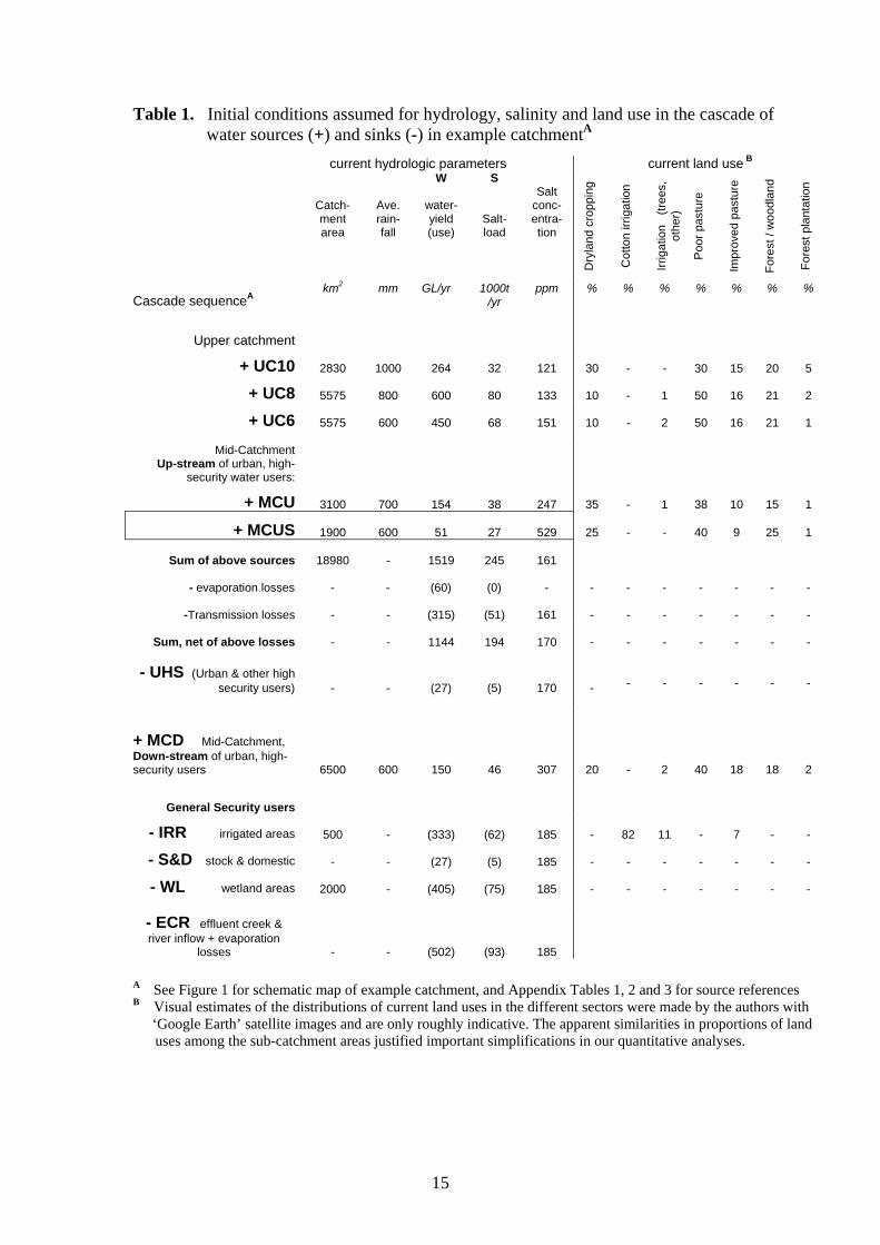
Table 1. Initial conditions assumed for hydrology, salinity and land use in the cascade of
water sources (+) and sinks (-) in example catchmentA
current hydrologic parameters current land use B
Catch-ment area
Ave. rain- fall
W
water-yield (use)
S
Salt-load
Salt
conc-entra-tion
Dry
land
cro
ppin
g
Cot
ton
irrig
atio
n
Irrig
atio
n (
trees
, ot
her)
Poo
r pas
ture
Impr
oved
pas
ture
Fore
st /
woo
dlan
d
Fore
st p
lant
atio
n
Cascade sequenceA km2
mm GL/yr
1000t
/yr ppm % % % % % % %
Upper catchment
+ UC10 2830 1000 264 32 121 30 -
-
30
15
20
5
+ UC8 5575 800 600
80
133 10 -
1
50
16
21
2
+ UC6 5575 600 450
68
151 10 -
2
50
16
21
1
Mid-Catchment
Up-stream of urban, high-security water users:
+ MCU 3100 700 154 38 247 35 -
1
38
10
15
1
+ MCUS 1900 600
51
27 529 25 -
-
40
9
25
1
Sum of above sources
18980 -
1519
245
161
- evaporation losses - - (60) (0) - - - - - - - -
-Transmission losses - -
(315)
(51)
161 - -
-
-
-
-
-
Sum, net of above losses - -
1144
194
170 - -
-
-
-
-
-
- UHS (Urban & other high
security users) - - (27) (5) 170 - -
-
-
-
-
-
+ MCD Mid-Catchment, Down-stream of urban, high-security users 6500 600
150
46 307 20
-
2
40
18
18
2
General Security users
- IRR irrigated areas 500 - (333)
(62)
185 -
82
11 -
7
-
-
- S&D stock & domestic - - (27)
(5)
185 - -
-
-
-
-
-
- WL wetland areas 2000 - (405)
(75)
185 - -
-
-
-
-
-
- ECR effluent creek & river inflow + evaporation
losses - - (502)
(93)
185
A See Figure 1 for schematic map of example catchment, and Appendix Tables 1, 2 and 3 for source references B Visual estimates of the distributions of current land uses in the different sectors were made by the authors with ‘Google Earth’ satellite images and are only roughly indicative. The apparent similarities in proportions of land uses among the sub-catchment areas justified important simplifications in our quantitative analyses.

16
Table 2. Mass balance of WaterA and SaltB deliverable downstream given current FRESH conditions, as in Table 1, and for the hypothetical ‘SALTY’ scenario, which assumes a very salty sub-catchment (MCUS)
Delivered downstream Hypothetical case ( C )with current conditions with Salt x 20 from MCUS
Catchment area
Mean annual rainfall W S concentr. W S concentr.
km 2 mm GL 1000t/yr S t / GL GL 1000t/yr S t / GLUpper catchment tributaries (ppm ) (ppm )
+ UC10 2830 1000 199 25 127 199 25 127+ UC8 5575 800 452 63 140 452 63 140+ UC6 5575 600 339 54 159 339 54 159
Mid-Catchment tributaries upstream of urban, high-security water users+ MCU 3100 700 116 30 259 116 30 259
U Sum of tributaries upstream of UHS except for MUCS 1106 173 157 1106 173 157
+ MCUS (salty) 1900 600 38 21 557 38 428 11132Sum upstream of UHS 1144 194 170 1144 600 525
- UHS (Urban & other high security user) consumption:
-27 -5 170 -27 -14 525
+ MCD Mid-Catchment tributaries, Down-stream of urban, high-security users:6500 600 150 46 307 150 46 307
Sum, net of above (+, -) 1267 235 186 1267 632 499
General Security users downstream of UHS:
- IRR irrigated areas 500 - -333 -62 186 -333 -166 499
- S&D stock & domestic - - -27 -5 186 -27 -13 499
- WL wetland areas 2000 - -405 -75 186 -405 -202 499
- ECR effluent creek & river inflow & evaporation
losses - - -502 -93 186 -502 -250 499
A water yields of the upper and mid-catchment tributaries upstream of UHS were divided by a factor of 1.328 to account for transmission and evaporative loses B salt loads from the upper and mid-catchment tributaries upstream of UHS were divided by a factor of 1.263 to account for transmission loses; evaporative loses of water, however, leave the salt in the river. See Appendix Table 1b for loss estimates
The different policy settings explored with this simplified construction of the
catchment under ‘current’ FRESH conditions and hypothetical SALTY conditions are
given in Table 3.
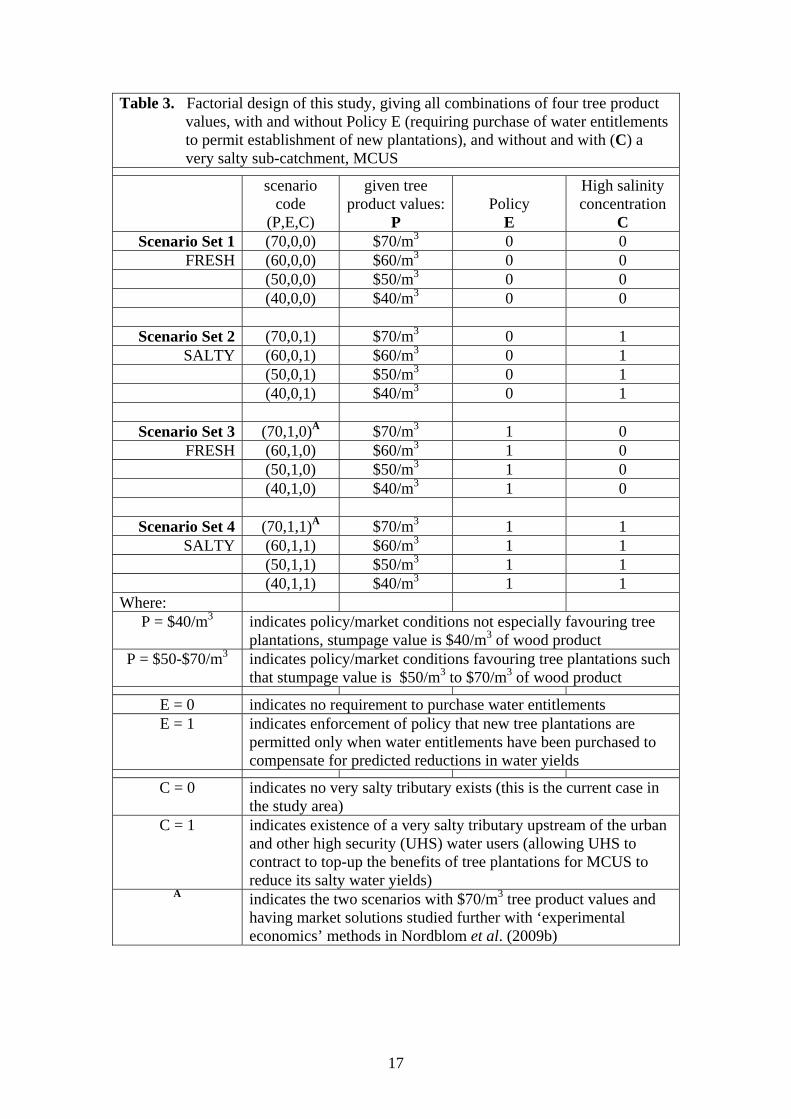
17
Table 3. Factorial design of this study, giving all combinations of four tree product
values, with and without Policy E (requiring purchase of water entitlements to permit establishment of new plantations), and without and with (C) a very salty sub-catchment, MCUS
scenario code
(P,E,C)
given tree product values:
P
Policy
E
High salinity concentration
C Scenario Set 1 (70,0,0) $70/m3 0 0
FRESH (60,0,0) $60/m3 0 0 (50,0,0) $50/m3 0 0 (40,0,0) $40/m3 0 0
Scenario Set 2 (70,0,1) $70/m3 0 1
SALTY (60,0,1) $60/m3 0 1 (50,0,1) $50/m3 0 1 (40,0,1) $40/m3 0 1
Scenario Set 3 (70,1,0)A $70/m3 1 0
FRESH (60,1,0) $60/m3 1 0 (50,1,0) $50/m3 1 0 (40,1,0) $40/m3 1 0
Scenario Set 4 (70,1,1)A $70/m3 1 1
SALTY (60,1,1) $60/m3 1 1 (50,1,1) $50/m3 1 1 (40,1,1) $40/m3 1 1
Where: P = $40/m3 indicates policy/market conditions not especially favouring tree
plantations, stumpage value is $40/m3 of wood product P = $50-$70/m3 indicates policy/market conditions favouring tree plantations such
that stumpage value is $50/m3 to $70/m3 of wood product
E = 0 indicates no requirement to purchase water entitlements E = 1 indicates enforcement of policy that new tree plantations are
permitted only when water entitlements have been purchased to compensate for predicted reductions in water yields
C = 0 indicates no very salty tributary exists (this is the current case in the study area)
C = 1 indicates existence of a very salty tributary upstream of the urban and other high security (UHS) water users (allowing UHS to contract to top-up the benefits of tree plantations for MCUS to reduce its salty water yields)
A indicates the two scenarios with $70/m3 tree product values and having market solutions studied further with ‘experimental economics’ methods in Nordblom et al. (2009b)
18
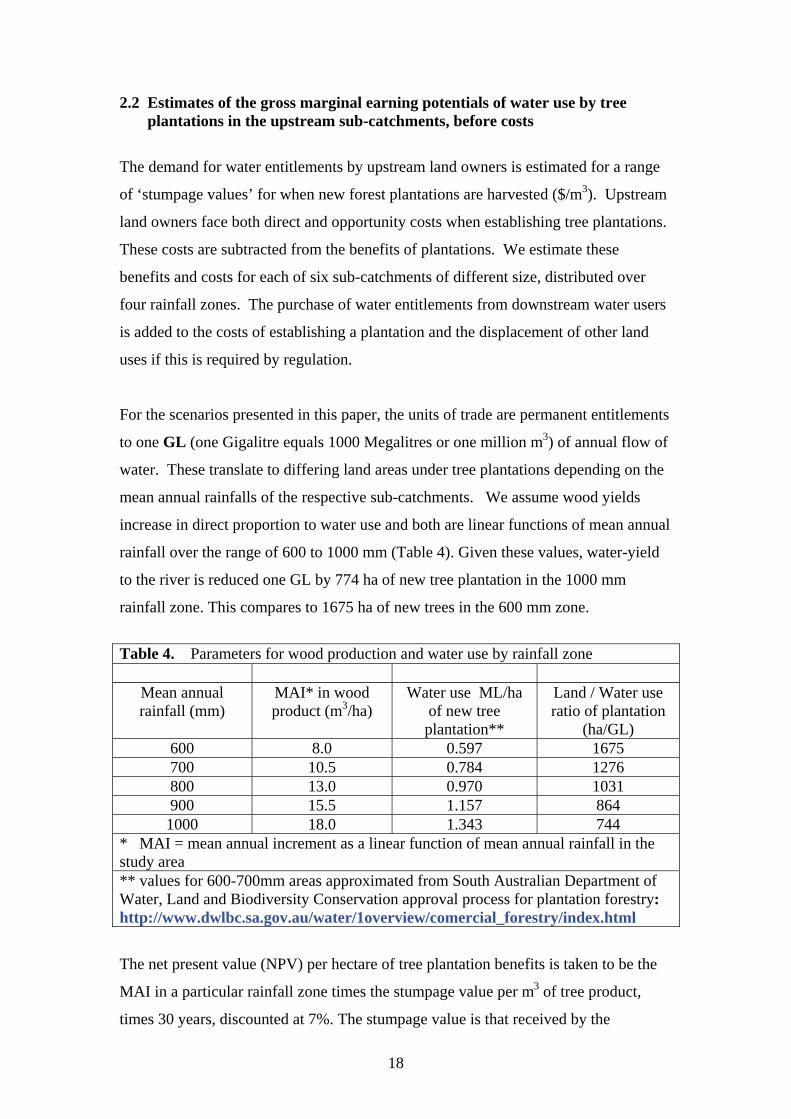
2.2 Estimates of the gross marginal earning potentials of water use by tree plantations in the upstream sub-catchments, before costs
The demand for water entitlements by upstream land owners is estimated for a range
of ‘stumpage values’ for when new forest plantations are harvested ($/m3). Upstream
land owners face both direct and opportunity costs when establishing tree plantations.
These costs are subtracted from the benefits of plantations. We estimate these
benefits and costs for each of six sub-catchments of different size, distributed over
four rainfall zones. The purchase of water entitlements from downstream water users
is added to the costs of establishing a plantation and the displacement of other land
uses if this is required by regulation.
For the scenarios presented in this paper, the units of trade are permanent entitlements
to one GL (one Gigalitre equals 1000 Megalitres or one million m3) of annual flow of
water. These translate to differing land areas under tree plantations depending on the
mean annual rainfalls of the respective sub-catchments. We assume wood yields
increase in direct proportion to water use and both are linear functions of mean annual
rainfall over the range of 600 to 1000 mm (Table 4). Given these values, water-yield
to the river is reduced one GL by 774 ha of new tree plantation in the 1000 mm
rainfall zone. This compares to 1675 ha of new trees in the 600 mm zone.
Table 4. Parameters for wood production and water use by rainfall zone
Mean annual rainfall (mm)
MAI* in wood product (m3/ha)
Water use ML/ha of new tree plantation**
Land / Water use ratio of plantation
(ha/GL) 600 8.0 0.597 1675 700 10.5 0.784 1276 800 13.0 0.970 1031 900 15.5 1.157 864 1000 18.0 1.343 744
* MAI = mean annual increment as a linear function of mean annual rainfall in the study area ** values for 600-700mm areas approximated from South Australian Department of Water, Land and Biodiversity Conservation approval process for plantation forestry: http://www.dwlbc.sa.gov.au/water/1overview/comercial_forestry/index.html
The net present value (NPV) per hectare of tree plantation benefits is taken to be the
MAI in a particular rainfall zone times the stumpage value per m3 of tree product,
times 30 years, discounted at 7%. The stumpage value is that received by the
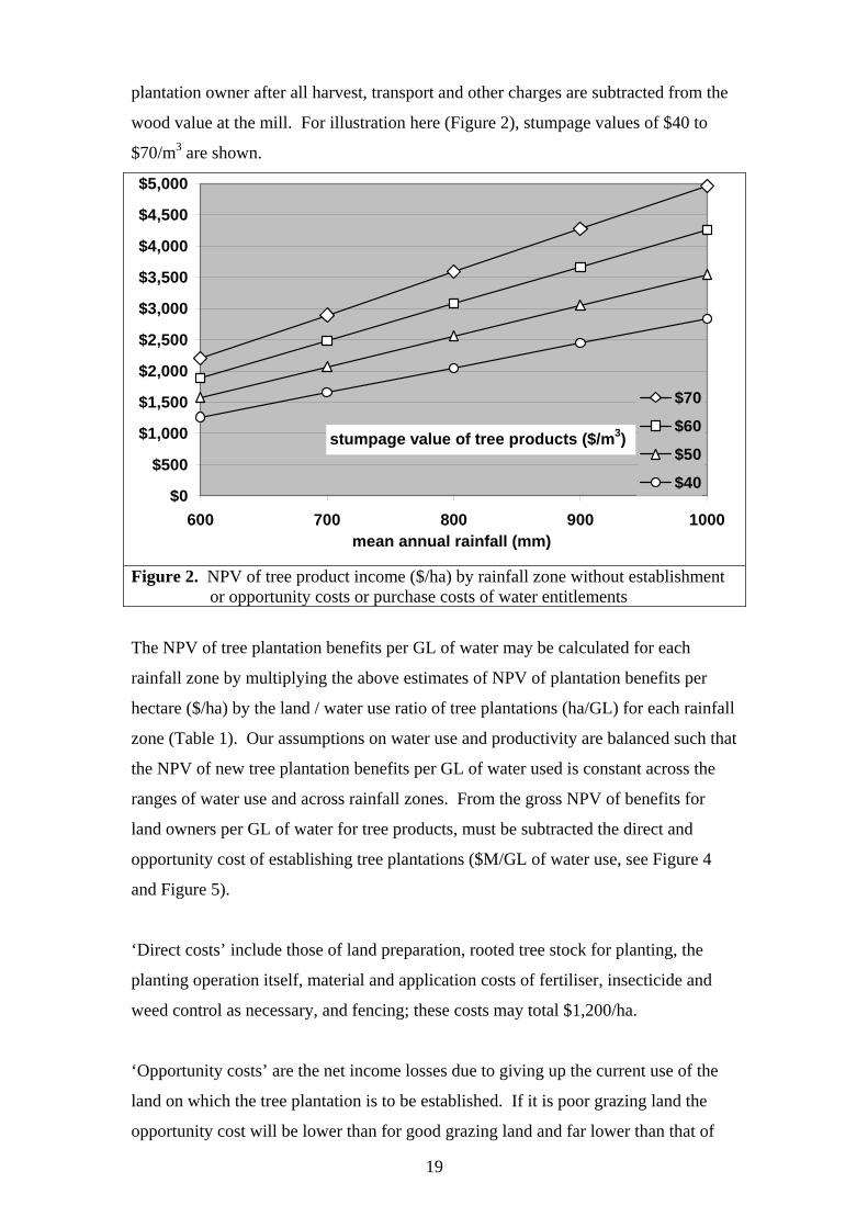
19
plantation owner after all harvest, transport and other charges are subtracted from the
wood value at the mill. For illustration here (Figure 2), stumpage values of $40 to
$70/m3 are shown.
$0
$500
$1,000
$1,500
$2,000
$2,500
$3,000
$3,500
$4,000
$4,500
$5,000
600 700 800 900 1000mean annual rainfall (mm)
$70
$60
$50
$40
stumpage value of tree products ($/m3)
Figure 2. NPV of tree product income ($/ha) by rainfall zone without establishment or opportunity costs or purchase costs of water entitlements
The NPV of tree plantation benefits per GL of water may be calculated for each
rainfall zone by multiplying the above estimates of NPV of plantation benefits per
hectare ($/ha) by the land / water use ratio of tree plantations (ha/GL) for each rainfall
zone (Table 1). Our assumptions on water use and productivity are balanced such that
the NPV of new tree plantation benefits per GL of water used is constant across the
ranges of water use and across rainfall zones. From the gross NPV of benefits for
land owners per GL of water for tree products, must be subtracted the direct and
opportunity cost of establishing tree plantations ($M/GL of water use, see Figure 4
and Figure 5).
‘Direct costs’ include those of land preparation, rooted tree stock for planting, the
planting operation itself, material and application costs of fertiliser, insecticide and
weed control as necessary, and fencing; these costs may total $1,200/ha.
‘Opportunity costs’ are the net income losses due to giving up the current use of the
land on which the tree plantation is to be established. If it is poor grazing land the
opportunity cost will be lower than for good grazing land and far lower than that of

20
productive farm land; these costs need to be considered where a newly established
tree plantation excludes other productive uses.
Derivation of Figure 4 began by summing the water-yields and salt-loads of clusters
a, b and c in Figure 3 (identified as the 2nd, 3rd & 4th groundwater salinity classes in
the Little River Catchment by Evans et al. 2004). Our linear programming analysis
solved for least-cost land use changes to meet specified targets for changes in water
and salt yields of the three classes of salt-source land (Figure 3). Our analysis
assumed that all present forest areas will be retained while new forest plantations,
even if not profitable in themselves, could be established to use water strategically for
salinity mitigation. It is technically feasible to increase water-yields and salt loads by
shifting land use away from perennial pastures and expanding annual pastures and
cropping. However, our analysis focuses on the water-yield reducing effects of tree
plantations.
2.3 Estimating marginal values of water for tree plantations, after counting direct and opportunity costs
Nordblom et al. (2006; 2007a,b; 2008a,b) explored the idea of minimising the direct
and opportunity costs of reducing salt loads in streams through strategic changes in
land use. A conclusion of that work, demonstrated again recently by Nordblom et al.
(2009a, 2010), is that the least-cost pathway for reducing salt-load entering a stream
from a catchment reaches an upper limit with new tree plantations replacing other
land uses.
New analyses by the authors for Little River Catchment in the Macquarie Valley,
NSW, have allowed us to plot such least-cost land use changes (Figure 3). The
aggregated raw economic results (of clusters a, b and c in Figure 3) from our linear
programming analyses for decreasing salt-loads and water-yields were smoothed by
fitting a cubic function. The smoothed results were further adjusted to match in scale
our catchment-wide water-yield and salt-load data for MCUS. They were adjusted
further for evaporative and transmission losses to represent ‘deliverable’ water yields
from MCUS (Figure 4).
The direct and opportunity costs of tree planting will depend on the land uses being
displaced. Inspection of satellite images of upstream areas compared with Little

21
River, a well-studied sub-catchment (Evans et al. 2004; Finlayson et al., 2007, 2010;
Hall et al., 2002; Murphy & Lawrie 1998; Nordblom et al. 2006) allowed estimates of
various proportions of land uses in the other sub-catchments (Table 1). Lacking better
estimates, these land use proportions appeared sufficiently similar to justify simply
scaling up the plantation cost curve (Figure 4), ‘stretching’ it horizontally to match the
relative ranges of water yield change in the other sub-catchments. The plantation cost
curve, based on the lowest (600mm) rainfall zone, was adjusted downward for the
higher rainfall zones, which need fewer hectares of plantation per GL of water used.
For example, we assume UC10 in the 1000mm rainfall zone requires only 744 ha of
new plantation to reduce water-yield to one GL below the base level from that area,
while in 600mm rainfall zones (such as UC6, MCUS and MCD) would need 1675 ha
of new plantation to have the same effect (Table 4). The UC10 plantation cost curve,
therefore, is reduced by a constant equal to the cost of the first GL unit from MCUS
minus 744/1675 of that same cost. Thus the cost curves for the 800 and 700 mm
zones (UC8 and MCU) are also adjusted downwards by constant amounts according
to the areas of tree plantations needed in each to reduce water-yields by one GL
relative to that of MCUS.
We assume the first GL of water used by new plantations in MCUS will have direct
and opportunity costs on the order of $2M/GL while the highest-cost plantations will
exceed $4.5M/GL in direct and opportunity costs. The latter cost figure is well above
the highest NPV of plantation benefits we consider (Figure 2), so the cost curve will
exceed or cut the benefit line in every case, providing a hard limit to the expansion of
such water use. However, in some cases this limit is very high.

22
0
10000
20000
30000
40000
50000
60000
-16
-15
-14
-13
-12
-11
-10 -9 -8 -7 -6 -5 -4 -3 -2 -1 0 +1 +2 +3 +4 +5
Land
-use
allo
catio
ns (h
a)
Crop & Past. Rotations (ha)
Naturalised Past, Poor (ha)
Naturalised Past, Better (ha)
Sown Perm. Pasture (ha)
Forest Plantation, new (ha)
Forest, Native (ha)
0
5000
10000
15000
20000
25000
30000
35000
40000
45000
-14
-13
-12
-11
-10 -9 -8 -7 -6 -5 -4 -3 -2 -1 0 +1 +2 +3
Land
-use
allo
catio
ns (h
a)
0
5000
10000
15000
20000
25000
30000
35000
40000
-9 -8 -7 -6 - 5 -4 -3 - 2 -1 0 +1 +2
Change in Water-yield (GL)
Land
-use
allo
catio
ns (h
a)
a
c
b
Figure 3. Least-cost land use changes to alter water-yields from three parts (a, b, c)
of Little River. Present land use is shown at the zero-change point in each case.
Subtracting the least-cost sequence of adding tree plantations to the landscape (Figure
4) from the benefits of plantations (horizontal lines) to landowners in this 600 mm
rainfall area allows us to express the marginal values of water used by plantations;
that is, their demand for water in $M/GL. For this, the horizontal axis may be labelled
“water use by plantations, GL/year” with the vertical axis being “marginal value of
water to plantation owner, $M/GL” (Figure 5).
23
0.000.250.500.751.001.251.501.752.002.252.502.753.003.253.503.754.004.254.504.75
0 1 2 3 4 5 6 7 8 9 10 11 12 13 14 15 16 17
reduction in mean annual water-yield from MCUS with new tree plantations (GL / year)
$m/G
L
$70
$60
$50
$40
MC ($m/GL)
Stumpage value of tree products, $/m3
$M/G
L
$M/GL
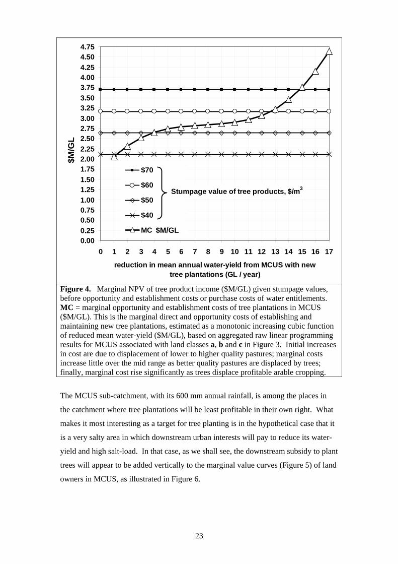
Figure 4. Marginal NPV of tree product income ($M/GL) given stumpage values, before opportunity and establishment costs or purchase costs of water entitlements. MC = marginal opportunity and establishment costs of tree plantations in MCUS ($M/GL). This is the marginal direct and opportunity costs of establishing and maintaining new tree plantations, estimated as a monotonic increasing cubic function of reduced mean water-yield ($M/GL), based on aggregated raw linear programming results for MCUS associated with land classes a, b and c in Figure 3. Initial increases in cost are due to displacement of lower to higher quality pastures; marginal costs increase little over the mid range as better quality pastures are displaced by trees; finally, marginal cost rise significantly as trees displace profitable arable cropping.
The MCUS sub-catchment, with its 600 mm annual rainfall, is among the places in
the catchment where tree plantations will be least profitable in their own right. What
makes it most interesting as a target for tree planting is in the hypothetical case that it
is a very salty area in which downstream urban interests will pay to reduce its water-
yield and high salt-load. In that case, as we shall see, the downstream subsidy to plant
trees will appear to be added vertically to the marginal value curves (Figure 5) of land
owners in MCUS, as illustrated in Figure 6.
24
0.000.25
0.500.75
1.001.25
1.501.75
2.002.25
0 1 2 3 4 5 6 7 8 9 10 11 12 13 14 15 16 17 18
water use by plantations (GL/year)mar
gina
l val
ue o
f wat
er to
pla
ntat
ion
owne
r ($
m/G
L)
$70$60$50
stumpage value of tree products, $/m3
( $M
/GL
)
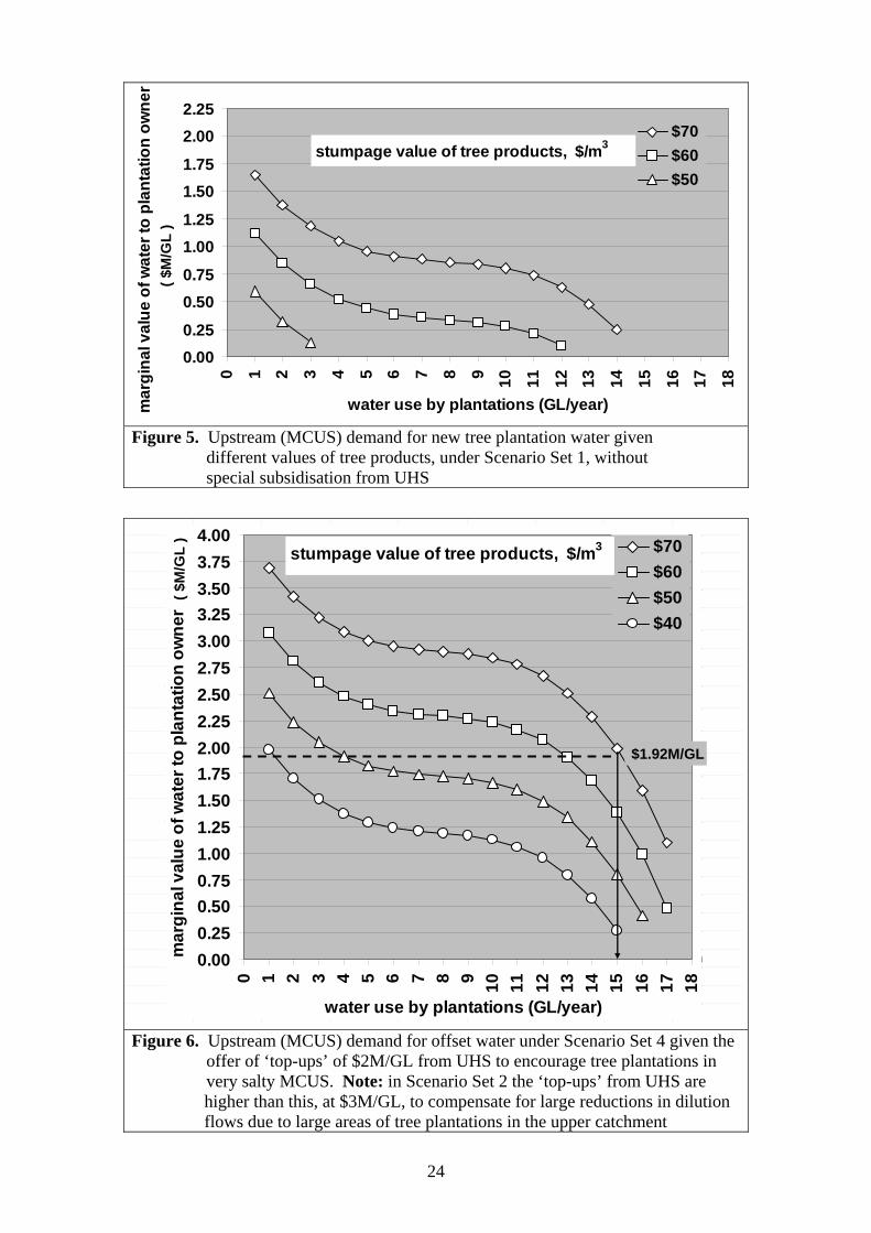
Figure 5. Upstream (MCUS) demand for new tree plantation water given different values of tree products, under Scenario Set 1, without special subsidisation from UHS
fresh IRR & S&D shares
$70 $50 28%: $70 $50Higher than current GL by:
10 83 72 23 20 23.24C8 182 150 51 42 50.96C6 120 24 34 7 33.6CU 45 35 13 10 12.6US 14 3 4 1 3.92
CD 53 11 15 3 14.84497 295 140 83
Lower than current GL by:D 11 6R 129 77
140 83Proposed initial endowments for SS3Uto start with mid and upper catchmentand with S&D and IRR holding less th0.00
0.250.500.751.001.251.501.752.002.252.502.753.003.253.503.754.00
0 1 2 3 4 5 6 7 8 9 10 11 12 13 14 15 16 17 18
water use by plantations (GL/year)
mar
gina
l val
ue o
f wat
er to
pla
ntat
ion
owne
r ($
m/G
L) $70$60$50$40
stumpage value of tree products, $/m3
$1.92m/GL
( $M
/GL
)
$1.92M/GL
Figure 6. Upstream (MCUS) demand for offset water under Scenario Set 4 given the offer of ‘top-ups’ of $2M/GL from UHS to encourage tree plantations in very salty MCUS. Note: in Scenario Set 2 the ‘top-ups’ from UHS are
higher than this, at $3M/GL, to compensate for large reductions in dilution flows due to large areas of tree plantations in the upper catchment
25
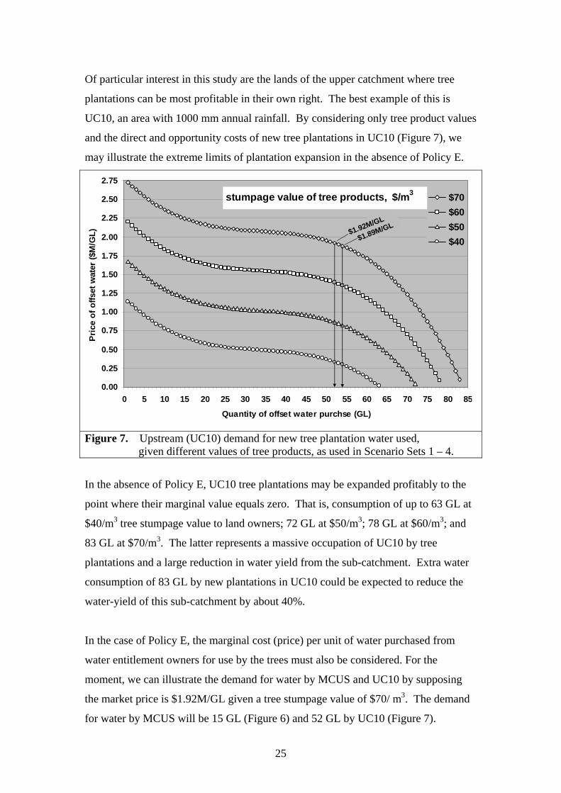
Of particular interest in this study are the lands of the upper catchment where tree
plantations can be most profitable in their own right. The best example of this is
UC10, an area with 1000 mm annual rainfall. By considering only tree product values
and the direct and opportunity costs of new tree plantations in UC10 (Figure 7), we
may illustrate the extreme limits of plantation expansion in the absence of Policy E.
0.00
0.25
0.50
0.75
1.00
1.25
1.50
1.75
2.00
2.25
2.50
2.75
0 5 10 15 20 25 30 35 40 45 50 55 60 65 70 75 80 85
Quantity of offset water purchse (GL)
Pric
e of
offs
et w
ater
($M
/GL)
$70$60$50$40
stumpage value of tree products, $/m3
$1.89M/GL$1.92M/GL
Figure 7. Upstream (UC10) demand for new tree plantation water used, given different values of tree products, as used in Scenario Sets 1 – 4.
In the absence of Policy E, UC10 tree plantations may be expanded profitably to the
point where their marginal value equals zero. That is, consumption of up to 63 GL at
$40/m3 tree stumpage value to land owners; 72 GL at $50/m3; 78 GL at $60/m3; and
83 GL at $70/m3. The latter represents a massive occupation of UC10 by tree
plantations and a large reduction in water yield from the sub-catchment. Extra water
consumption of 83 GL by new plantations in UC10 could be expected to reduce the
water-yield of this sub-catchment by about 40%.
In the case of Policy E, the marginal cost (price) per unit of water purchased from
water entitlement owners for use by the trees must also be considered. For the
moment, we can illustrate the demand for water by MCUS and UC10 by supposing
the market price is $1.92M/GL given a tree stumpage value of $70/ m3. The demand
for water by MCUS will be 15 GL (Figure 6) and 52 GL by UC10 (Figure 7).

26
The price of water in such cases is determined in the competitive market given the
marginal values of those wishing to purchase water and those of the downstream
water entitlement holders. We now need to construct estimates of the marginal values
of water for the downstream entitlement holders.
2.4 Marginal values of water use by irrigators and stock & domestic water
users starting with recent prices of permanent water entitlement trades We visualise the marginal values for water by IRR and S&D sectors as downward-
sloping demand curves passing through the value of $1.2M/GL, a recent price for
permanent trades, at the current entitlement levels of 333 and 27 GL, respectively
(Table 2, Figure 8). This construction supposes that IRR and S&D would be willing
to purchase more water at lower prices (e.g., 100 and 10 GL, respectively at
$0.4M/GL) and to sell water at higher prices. It also supposes the WL sector,
representing the government’s environmental interests would offer to purchase up to
15 GL of water at a fixed price of $1.33M/GL (above recent prices of permanent
trades), but not be willing to sell any of its entitlements for less than $3.86M/GL, just
above the price at which IRR would be willing to sell its last unit of entitlement. This
high reserve price by WL could be taken as that at which offsetting alternative
wetland assets could be secured and developed. These scenarios also assume full
100% allocations of these entitlements with no year-to-year variations, and that all
entitlements are held by these downstream interests and UHS which has a fixed
entitlement of 27 GL. We also assume UHS is not interested in selling water or
buying water for its own use. These assumptions, being somewhat arbitrary in
marginal rates, are anchored to historical values of the downstream water market and
comprise a simple and transparent scenario with which we may consider physical and
economic interactions with the upper catchment water sources.
This construction, with downstream sectors holding all available entitlements puts
these sectors in the position of the only potential suppliers of water entitlements in the
case that Policy E is in force and upstream land owners are obliged to purchase water
entitlements to permit the establishment of tree plantations. Alternatively, if
widespread establishment of new tree plantations takes place in the absence of Policy
E, the downstream entitlement holders will suffer losses as their allocations of water
are reduced. We assume such losses (in GL) would be in proportion to their
27
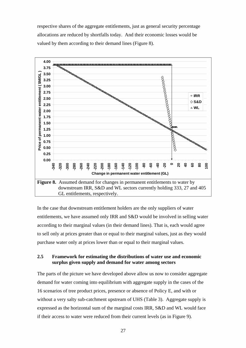
respective shares of the aggregate entitlements, just as general security percentage
allocations are reduced by shortfalls today. And their economic losses would be
valued by them according to their demand lines (Figure 8).
0.000.250.500.751.001.251.501.752.002.252.502.753.003.253.503.754.00
-340
-320
-300
-280
-260
-240
-220
-200
-180
-160
-140
-120
-100 -8
0
-60
-40
-20 0 20 40 60 80 100
Change in permanent water entitlement (GL)
Pric
e of
per
man
ent w
ater
ent
itlem
ent (
$M
/GL
)
IRRS&DWL
Figure 8. Assumed demand for changes in permanent entitlements to water by downstream IRR, S&D and WL sectors currently holding 333, 27 and 405 GL entitlements, respectively.
In the case that downstream entitlement holders are the only suppliers of water
entitlements, we have assumed only IRR and S&D would be involved in selling water
according to their marginal values (in their demand lines). That is, each would agree
to sell only at prices greater than or equal to their marginal values, just as they would
purchase water only at prices lower than or equal to their marginal values.
2.5 Framework for estimating the distributions of water use and economic
surplus given supply and demand for water among sectors The parts of the picture we have developed above allow us now to consider aggregate
demand for water coming into equilibrium with aggregate supply in the cases of the
16 scenarios of tree product prices, presence or absence of Policy E, and with or
without a very salty sub-catchment upstream of UHS (Table 3). Aggregate supply is
expressed as the horizontal sum of the marginal costs IRR, S&D and WL would face
if their access to water were reduced from their current levels (as in Figure 9).

28
Aggregate demand for water for new upstream tree plantations may be expressed as
the horizontal sum of the individual sub-catchment demands (as in Figure 10 for the
FRESH scenarios). The irregular ‘wavy’ character of these curves is due to the nature
of their constituent sub-catchment curves (i.e., Figure 6 and Figure 7). Assembling
the marginal value arrays of the constituent sectors in a column with a paired column
identifying sector names, allows sorting the columns in descending order by marginal
values, creating the ‘horizontal sum’ to represent the demand curve. A similarly
constructed supply curve in ascending order is matched to find the equilibrium price.
Then, up to that point, the demand and supply arrays are each sorted by source. The
number of GL and the sum of marginal values from each source are the values listed
as GL purchased (or sold), and economic surpluses (or losses) in Tables 5 – 8.
0.00
0.25
0.50
0.75
1.00
1.25
1.50
1.75
2.00
2.25
2.50
2.75
3.00
3.25
3.50
3.75
4.00
4.25
0 10 20 30 40 50 60 70 80 90 100
110
120
130
140
150
160
170
180
190
200
210
220
230
240
250
260
270
280
290
300
310
320
330
340
350
360
370
380
390
Supply of permanent water entitlements (GL)
Agg
rega
te s
uppl
y pr
ice
($M
/GL)
IRRS&DWL
Figure 9. Aggregate supply of downstream water entitlements… of interest in the presence of Policy E where upstream landowners would need to purchase water entitlements to permit establishment of new tree plantations
29
0.00
0.25
0.50
0.75
1.00
1.25
1.50
1.75
2.00
2.25
2.50
2.75
0 50 100 150 200 250 300 350 400 450 500
water purchase to 'offset' use by new tree plantations (GL)
Pric
e of
'offs
et' w
ater
( $M
/GL
)
$70$60$50$40
y
Demand for water by plantations given stumpage value of tree products ($/m3)
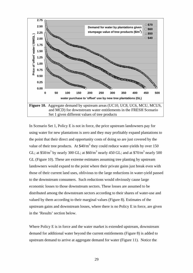
Figure 10. Aggregate demand by upstream areas (UC10, UC8, UC6, MCU, MCUS, and MCD) for downstream water entitlements in the FRESH Scenario Set 1 given different values of tree products
In Scenario Set 1, Policy E is not in force, the price upstream landowners pay for
using water for new plantations is zero and they may profitably expand plantations to
the point that their direct and opportunity costs of doing so are just covered by the
value of their tree products. At $40/m3 they could reduce water-yields by over 150
GL; at $50/m3 by nearly 300 GL; at $60/m3 nearly 450 GL; and at $70/m3 nearly 500
GL (Figure 10). These are extreme estimates assuming tree planting by upstream
landowners would expand to the point where their private gains just break even with
those of their current land uses, oblivious to the large reductions in water-yield passed
to the downstream consumers. Such reductions would obviously cause large
economic losses to those downstream sectors. These losses are assumed to be
distributed among the downstream sectors according to their shares of water-use and
valued by them according to their marginal values (Figure 8). Estimates of the
upstream gains and downstream losses, where there is no Policy E in force, are given
in the ‘Results’ section below.
Where Policy E is in force and the water market is extended upstream, downstream
demand for additional water beyond the current entitlements (Figure 8) is added to
upstream demand to arrive at aggregate demand for water (Figure 11). Notice the
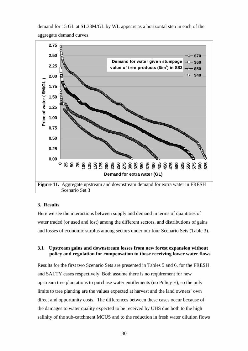
30
demand for 15 GL at $1.33M/GL by WL appears as a horizontal step in each of the
aggregate demand curves.
0.00
0.25
0.50
0.75
1.00
1.25
1.50
1.75
2.00
2.25
2.50
2.75
0 25 50 75 100
125
150
175
200
225
250
275
300
325
350
375
400
425
450
475
500
525
550
575
600
625
Demand for extra water (GL)
Pric
e of
wat
er (
$M/G
L )
$70$60$50$40
Demand for water given stumpage value of tree products ($/m3) in SS3
Figure 11. Aggregate upstream and downstream demand for extra water in FRESH Scenario Set 3
3. Results
Here we see the interactions between supply and demand in terms of quantities of
water traded (or used and lost) among the different sectors, and distributions of gains
and losses of economic surplus among sectors under our four Scenario Sets (Table 3).
3.1 Upstream gains and downstream losses from new forest expansion without policy and regulation for compensation to those receiving lower water flows
Results for the first two Scenario Sets are presented in Tables 5 and 6, for the FRESH
and SALTY cases respectively. Both assume there is no requirement for new
upstream tree plantations to purchase water entitlements (no Policy E), so the only
limits to tree planting are the values expected at harvest and the land owners’ own
direct and opportunity costs. The differences between these cases occur because of
the damages to water quality expected to be received by UHS due both to the high
salinity of the sub-catchment MCUS and to the reduction in fresh water dilution flows

31
from the other upstream sub-catchments. In this case we assume UHS will pay
$3M/GL for water yield reductions from a very salty MCUS through planting trees
there (see Appendix Tables 4 and 5 for calculations). From the viewpoint of MCUS
this is a substantial ‘top-up’ of their demand curves (Figure 5 and 6).
Tables 5 and 6 are each divided into estimates of gains to the upstream sub-
catchments and losses to the downstream sectors, in terms of changes in water used
and changes in economic surpluses. Because in these scenarios there is no market to
balance the economic surpluses and compensate losses in these changes, the upstream
sectors are the big winners and the downstream consumers are the big losers. Higher
values for tree products magnify these disparities substantially.
In our text about upstream new plantation demand for ‘free’ water (Figure 10) the
mentioned quantities (GL) of water that would be used were the maximum that may
be taken with the smallest net benefit to upstream land owners. Somewhat smaller
quantities would be used by new plantations if these land owners set a minimum
margin of net gain not at zero but at $0.2M/GL. This was the cut-off level for the
totals reported in Tables 5 and 6, where there is no market constraint on water use.

32
Table 5. Economic results of Scenario Set 1, with fresh water flows from all sub- catchments and no Policy E (that is, no requirement for those establishing new tree plantations to purchase downstream water entitlements)
a. Gains to water-source catchment areas from expanding tree plantations, assuming no payments are required for extra water use
with tree product values ($/m3)
with tree product values ($/m3)
$70 $60 $50 $40 $70 $60 $50 $40
Sector Water yield reduction (GL/yr)
Gains in surpluses ($M)B
UC10 82 76 69 57 151 108 69 32 UC8 178 163 140 45 274 181 96 19 UC6 114 87 12 99 40 4 MCU 44 39 30 4 57 34 13 1 MCUS 14 11 2 13 5 1 MCD 51 39 5 44 18 2
space space Totals 483 415 258 106 639 386 185 53 b. Losses faced by downstream water users due to unilateral reductions in upstream water yields, assuming water losses are distributed in proportion to current water use
Current flowsA
given tree product
values ($/m3)
with uncompensated reductions in water flow given tree product values
($/m3) Sector GL share $70 $60 $50 $40 $70 $60 $50 $40
Lost water availability (GL/yr)
Imposed losses of surplus ($M)C
- IRR irrigated
areas
333 26% 127 109 68 28 217 179 100 37
- S&D stock &
domestic
27 2% 10 9 5 2 16 14 7 3
- WL wetland
areas
405 32% 154 133 82 34 595 514 317 131
- ECR D 502 40% 191 164 102 42 0 0 0 0
Totals 1267 100% 483 415 258 106 829 707 424 171
A values from Table 2 B cumulative sum of marginal benefits for increments in water use by upstream sectors for new tree plantations C cumulative sum of marginal costs for decrements in water availability for IRR, S&D and WL
D ECR = effluent creek & river inflow & evaporation losses. Changes in water flow to ECR are not assigned economic values here Note: There is no impact on UHS which has high security entitlements, "fresh" water and is assumed always to receive its full amount of 27 GL
33
Table 6. Economic results of Scenario Set 2, with very salty sub-catchment MCUS, and no Policy E, UHS toping-up MCUS benefits of tree plantations for salinity relief a. Gains to water-source catchment areas from expanding tree plantations assuming no payments are required for their extra water use
with tree product values ($/m3)
with tree product values ($/m3)
Sector $70 $60 $50 $40 $70 $60 $50 $40
Water yield reduction (GL/yr)
Gains in surpluses ($M)B
UC10 82 76 69 57 151 108 69 32 UC8 178 163 140 45 274 181 96 19 UC6 115 87 12 100 40 4 MCU 44 39 29 4 57 34 13 1 MCUS 17 17 17 16 62 50 36 22
share share MCD 51 39 5 44 18 2 Totals 487 421 272 122 688 431 219 76
b. Losses faced by downstream water users due to uncompensated reductions in upstream water yields, assuming water losses are distributed in proportion to current water use
Current flows A
given tree product values ($/m3)
given tree product values ($/m3)
Sector GL % share
$70 $60 $50 $40 $70 $60 $50 $40
Reduced water availability (GL/yr)
Imposed losses of surplus ($M)C
- IRR irrigated
areas
333 26% 128 111 71 32 220 183 106 43
- S&D stock &
domestic
27 2% 10 9 6 3 16 14 9 4
- WL wetland
areas
405 32% 156 135 87 39 603 522 336 151
- ECR D 502 40% 193 167 108 48 0 0 0 0
Totals 1267 100% 487 421 272 122 839 719 451 197
A values from Table 2 B cumulative sum of marginal benefits for increments in water use by upstream sectors for new tree plantations C cumulative sum of marginal costs for decrements in water availability for IRR, S&D and WL
D ECR = effluent creek & river inflow & evaporation losses. Changes in water Flow to ECR are not assigned economic values here Note: Differs from Scenario 1 (Table 5) as UHS ‘tops up’ benefits of MCUS for reducing water-yields and salt concentration given reduced fresh dilution flows from the upper catchment
34
The effects of increases in earning power of new forest plantations ($40 to $70/m3)
are quite dramatic in the absence of regulatory or market limitations on expansion
(Tables 5 & 6). Large amounts of water are used, and large economic surpluses
captured, by the upstream sectors. In these scenarios we project equally large
reductions in water flow to the downstream sectors. Assuming these losses would be
shared among the downstream sectors in proportion to their current entitlements, large
economic declines are projected for the IRR and S&D sectors, while environmental
declines can be expected in the WL and ECR sectors. We have put a price on the WL
losses, unsure whether this would be sufficient to replace the environmental
functionality with replacement and/or renovations elsewhere. We have not priced the
ECR losses, which presumably include some contributions to the Darling River.
3.2 Upstream and downstream surpluses from new forest expansion with policy and regulation enabling water trade from downstream to upstream
With an extended water market, results indicate establishment of smaller areas of
forest and compensation for lost water; so all sectors benefit (Tables 7 & 8). We
assume water trading is only from the IRR and S&D sectors, while current
entitlements continue to be fulfilled to the WL and ECR sectors. With Policy E, water
use by new tree plantations in the upstream sectors is much lower than the free water
scenarios (Tables 5 and 6). Further, under Policy E, new plantations are limited to
those parts of the catchment where they are most profitable in their own rights. In
Scenario Set 4 (Table 8) MCUS is offered subsidies of $2M/GL by UHS to plant trees
for reduced salt-water yields. The calculated subsidy offer from UHS is lower than in
Scenario Set 2 ($3M/GL) because the areas of new plantations and their water use are
substantially smaller than in the ‘free water’ case. That is, most of the former fresh
dilution flows continue in the case where a market price has to be paid for water used
by new tree plantations.
The idea that new tree plantations should be prevented by regulation is discounted by
our results. If our assumptions are approximately correct, the benefits of trading 90
GL of water from downstream uses to upstream plantations are on the order of $138M
and $192M to those sectors, respectively, in the FRESH case with the highest value
tree products (Table 7). In the SALTY case (Table 8) the downstream and upstream
surpluses are expected to be higher at $151M and $220M, respectively, as seven

35
Table 7. Economic results of Scenario Set 3, with fresh water from all sub- catchments and Policy E in force (water use by new tree plantations must be covered by purchase of existing downstream water entitlements) a. Water entitlements sold by downstream sectors
given tree product values
($/m3): given tree product values ($/m3):
$70 $60 $50 $40 $70 $60 $50 $40
Sector
Amount of water supplied (GL) Gains in surpluses ($M)
IRR 82 43 16 14 126 59 20 18 S&D 8 4 1 1 13 6 1 1
Totals 90 47 17 15 138 65 22 19 Equilibrium water price ($M/GL): 1.89 1.55 1.33 1.33
b. Water demand from sectors purchasing water
given tree product values ($/m3)
given tree product values ($/m3):
$70 $60 $50 $40 $70 $60 $50 $40
Sector Amount of water purchased (GL/yr)
Gains in surpluses ($M)
UC10 54 32 9 117 56 13 UC8 33 15 69 26 MCU 3 6 WL 8 15 11 20
Totals 90 47 17 15 192 82 24 20 Equilibrium water price ($M/GL): 1.89 1.55 1.33 1.33
0.00
0.25
0.50
0.75
1.00
1.25
1.50
1.75
2.00
2.25
2.50
2.75
0 5 10 15 20 25 30 35 40 45 50 55 60 65 70 75 80 85 90 95 100
Water traded (GL)
Pric
e of
wat
er ($
M/G
L)
$70$60$50$40Supply
Demand for water given stumpage value of tree products ($/m3) in Scenario Set 3
Figure 12. Aggregate upstream and downstream demand for extra water intersecting
with aggregate downstream supply of water from the IRR and S&D sectors in the FRESH Scenario Set 3

36
Table 8. Economic results of Scenario Set 4, with very salty MCUS, Policy E and UHS ‘topping up’ MCUS benefits from tree plantations for salinity mitigation
a. Water entitlements sold by downstream sectors
given tree product values ($/m3): given tree product values ($/m3): Sector $70 $60 $50 $40 $70 $60 $50 $40
Amount of water supplied (GL) Gains in surpluses ($M) IRR 89 48 19 16 139 67 24 20 S&D 8 4 1 1 12 6 1 1 Totals 97 52 20 17 151 73 26 22 Equilibrium water price ($M/GL): 1.92 1.59 1.37 1.33
b. Water demand sectors purchasing water
given tree product values ($/m3): given tree product values ($/m3): $70 $60 $50 $40 $70 $60 $50 $40
Amount of water purchased (GL) Gains in surpluses ($M)
Sector
UC10 52 25 8 114 45 12 UC8 28 13 59 22 MCU 2 4 MCUS 15 14 12 4 43 33 22 7 WL 13 17 Totals 97 52 20 17 220 100 34 24 Equilibrium water price ($M/GL): 1.92 1.59 1.37 1.33
0.00
0.25
0.50
0.75
1.00
1.25
1.50
1.75
2.00
2.25
2.50
2.75
3.00
3.25
3.50
3.75
0 5 10 15 20 25 30 35 40 45 50 55 60 65 70 75 80 85 90 95 100
water traded (GL)
Pric
e of
wat
er ($
M/G
L)
Supply$70$60$50$40
Demand for water given stumpage value of tree products ($/m3) in Scenario Set 4
Figure 13. Aggregate upstream and downstream demand for extra water intersecting
with aggregate downstream supply of water from the IRR and S&D sectors when UHS tops up benefits to MCUS for reducing water yield in SALTY Scenario Set 4

37
further GL of water are traded. These seven, plus eight GL drawn away from tree
planting elsewhere, make up the subsidised 15 GL purchased by MCUS in contrast to
zero in the FRESH case where UHS has no need to deal with salinity. Between the
FRESH and SALTY cases the price of water increases from $1.89M to $1.92M/GL.
4. Discussion and conclusions
In the ‘free water’ FRESH and SALTY cases of Scenario Sets 1 and 2 (Tables 5 & 6),
total upstream surpluses due to tree planting are $639M and $688M, respectively.
These are contrasted with downstream losses on the order of $829M and $839M,
respectively. Counting downstream losses to the aggregate of the IRR and S&D
sectors, these add up to $233M and $236M in the FRESH and SALTY cases,
respectively, given uncompensated losses of 137 and 138 GL of water flow to them;
further, uncompensated losses of 154 and 156 GL in annual river flow would be
suffered by the wetlands.. How do these scenarios of ‘free water’ for tree plantations
compare with Scenario Sets 3 and 4 (Tables 7 & 8) in which new tree plantations
must enter the market for the water they use?
With the requirement to purchase water for establishing new tree plantations,
upstream surpluses are projected to be $192M and $220M in the FRESH and SALTY
cases, respectively, while downstream sums of IRR and S&D surpluses are $138M
and $151M, given 90 and 97 GL of water traded upstream (Tables 7 & 8). In these
scenarios, trading and water use changes are assumed only among the downstream
(IRR and S&D) sectors and the six upstream sub-catchments, such that flows to the
wetlands are preserved. Greater surpluses in the hypothetical SALTY cases are due to
subsidies paid by UHS for tree planting to reduce water yields from the very salty
sub-catchment, thereby lowering river salinity to acceptable levels for domestic use.
Do the large potential upstream surpluses in the ‘free water’ Scenario Sets 1 & 2
outweigh the smaller downstream economic losses? Surely, from the viewpoint of the
downstream sectors, the answer is “no”.
Can we make the case that the ‘extended market’ Scenario Sets 3 & 4 (Tables 7 & 8)
produces more efficient, equitable and environmentally friendly results than the ‘free
water’ Scenario Sets 1 & 2 (Tables 5 & 6)?

38
● Yes, if ‘efficient’ means water going to various uses in which its marginal
values are equal… such that no high value uses are starved for water while it is
‘employed’ in lower value uses.
● Yes, if ‘equitable’ means no sector’s access to water is appropriated by
another without compensation, but water is traded at mutually agreeable prices
or not at all.
● Yes, if ‘environmentally friendly’ means water entitlements for riparian
habitats and wetlands are protected and honoured. Where adjustments to these
entitlements are judged necessary, the state may enter the market to do so.
Our assumptions regarding land uses, the direct and opportunity costs of planting
large areas of trees in the different areas and the downstream demands for water may
all be challenged, though there is little doubt the directions of change presented are
correct.
The consequences of higher marginal values for water by the downstream IRR and
S&D sectors are clear… their aggregate water supply line would simply cut the
aggregate demand curves at higher prices and result in lower quantities traded than in
the cases of Scenario Sets 3 & 4 (Tables 7 & 8). In the ‘free water’ Scenario Sets 1 &
2 (Tables 5 & 6), higher marginal values of water by the IRR and S&D sectors would
simply mean greater losses to them.
The changes in water yields are presented as if they are instantaneous with the
establishment of tree plantations, whereas we do expect water-yields to gradually
decline to a lower steady state over a number of years. We have dealt with such time
issues by using NPVs and permanent water trade prices, both capturing the long-run.
We have made GL of water the metric of trade because it is a common denominator
already for downstream water trade and readily translated into particular surface areas
of forest, as a function of annual rainfall.
We have developed a static model based on long-run rainfall figures, without concern
for historical year-to-year variations and droughts, or climate change. With respect to
the latter challenge, however, this study should give pause to the popular notion that
39
the obvious ‘right’ response is for us to plant lots of forest, here on the driest
continent.
We have noted two simplifying assumptions in our methods: (1) that mean annual
rainfalls, which range from 1000mm to 300mm in different parts of the catchment,
hold constant over time with no year-to-year variation and (2) that land use changes
are reflected quickly in changed catchment water-yield and salt-load. This means all
our point estimates of water-yield and salt-load changes are uncertain, within
unspecified probabilistic clouds and smeared across time. On one hand, this may
suggest it is a folly to ‘fine tune’ land use in a catchment to achieve small changes in
salt-loads and water-yields. On the other hand, the negative impact on water-yields
due to large increases in forest areas appears potentially large and relatively certain.
The two sources of variance in water-yields noted above raise challenges for the
accounting and trading of up-stream and downstream water rights. For example, if
downstream interests wish to alter the environmental services flowing from a
catchment by inducing certain land use changes there, the outcomes are necessarily
uncertain. Another example is the attribution of culpability for reduced catchment
water yields to new tree plantations; this is a classic case of externality damages but
heavily obscured by year-to-year variations in rainfall, non-uniform hydrologic
response times, as well as uncertainties in “climate change” (Nordblom et al. 2009a,
2010).
While mainly about water, this study incorporates concerns for river salinity and a
way those in an Urban area (UHS) most troubled by it (in a hypothetical case) could
deal with the problem presented by a sub-catchment seeping lots of salt into their
otherwise fresh water source. They could ‘top up’ the benefits land owners may have
from planting trees, thereby reducing water-yields from that particular area. An
alternative option for UHS in the hypothetical SALTY scenario could be to construct
a water pipeline directly to the most reliable fresh water source.
We have presented abstract upstream and downstream sectors, which are in reality
each constituted by many individual decision makers, as if they are single decision
makers each acting ‘rationally’ only for their individual best advantage.
40
The present model constructs simple economic profiles of each sector then given
several tree-product values calculates the equilibrium results expected when these
sectors interact. There are several clear conclusions that may be framed as answers to
the questions posed at the start of this paper:
● Could policies and programs that encourage large-scale forestry expansion
have the unintended effect of drying up important fresh water sources in
Australia, the driest continent? Clearly, yes.
● Should this happen, would the most disadvantaged be general-security water
entitlement holders (irrigators, stock & domestic users and vulnerable wet-
land environmental assets)? Clearly, yes.
● And would urban and other high-security users receive saltier water supplies
with high mitigation costs? Only in the case where a very salty sub-catchment
is located up-stream of these users who would suffer from reduced fresh
dilution flows and increased river salinity. Such a case has been posed
hypothetically in this study to demonstrate this effect.
● Could a policy requiring purchase of existing water entitlements to permit
establishment of forestry plantations help promote the most efficient
allocations of this finite resource among competing users? Such a system has
been implemented in southeast South Australia. Our study shows how
extending the water market from current downstream water users (urban, stock
& domestic and irrigators) to interests wishing to establish new forest
plantations in the upper catchment could result in a balance that is more
efficient, equitable and environmentally friendly than the case where new
forests are not required to obtain water entitlements.
Does it matter that we have assumed all water entitlements are initially only in the
hands of downstream sectors? Probably, but in the direction of less water trade than
predicted in this supply and demand analysis. Nordblom et al. (2009b) treat this
question explicitly. Coase (1960) posited that property rights will be sorted out
optimally with trade, regardless of the distribution of initial endowments, except
where there are high transaction costs.
Effective policy and regulation minimising transaction costs could facilitate trade of
water rights to new upstream forest plantations. Young & McColl (2009) have
reasoned that if entitlement and allocation regimes are set up in ways that have
41
hydrological integrity, the system “can autonomously adjust to climatic shifts,
changes in prices and changes in technology without compromising environmental
objectives”.
Does it matter that we have assumed (in SS3 and SS4, the market scenarios) general
security water entitlements are the same as high security water entitlements,
expressing rights to exact volumes of water to the entitlement holder each year and
tradable as such? There is no doubt that general security water entitlements, which
receive only allocated shares of their denominated volumes according to the rainfall
and storage levels that differ from year to year (as in SS1 and SS2) will present results
varying from those shown.
However, trade in entitlements for fixed volumes or probabilistic volumes of water
can be reconciled with a premium on certainty (or discounts for uncertainty).
Adamson et al. (2007) have provided an example of how to do this, but did not
include new forest plantations in the market for water. The present study provides
missing details that would allow a fuller analysis.
References Adamson, D., Thilak Mallawaarachchi, T., Quiggin, J. (2007), Water use and salinity in the Murray–Darling Basin: A state-contingent model. The Australian Journal of Agricultural and Resource Economics, 51, 263–281. Alexander, F. and Heaney, A. (2003), Potential Impact of Saline Irrigation Water on the Grape Industry in the Murray Darling Basin, Final Report to the Grape and Wine Research and Development Corporation, ABARE eReport 03.6, Canberra, April. (accessed 11 May 2010) http://www.abare.gov.au/publications_html/crops/crops_03/er03_irrigation.pdf Beale, G.T.H., Beecham, R., Harris, K., O'Neill, D., Schroo, H., Tuteja, N.K., Williams, R.M. (2000), Salinity predictions for NSW rivers within the Murray-Darling Basin. Centre for Natural Resources, NSW Department of Land and Water Conservation. 10 Valentine Ave, Parramatta NSW 2150. (accessed 11 May 2010) http://www.environment.nsw.gov.au/resources/salinity/salinitypredictions.pdf Bell, R. (2002), Capturing benefits from water entitlement trade in salinity affected areas: A role for trading houses? Australian Journal of Agricultural and Resource Economics, 46 (3): 347–366. Bell, R. and Beare, S. (2000), Salinity targets in the Murray-Darling Basin, Australian Commodities 7, 348-356. (accessed 11 May 2010) http://www.abare.gov.au/publications_html/ac/ac_00/ac00_june.pdf
42
Bell, R. and Heaney, A. (2001), A basin scale model for assessing salinity management options: model documentation. ABARE Technical Working Paper 2001.A. Canberra. Bennett, D. & Thomas, J.F. (Eds.). (1982), On rational grounds: systems analysis in catchment land use planning. Elsevier Scientific Publishing Co., Amsterdam Bennett, J. (2002), Choice Modelling Research Reports, Crawford School of Economics and Government, The Australian National University, Canberra (accessed 11 May 2010) http://www.crawford.anu.edu.au/staff/jb_chmdrr.php Binning, C., Baker, B., Meharg, S., Cork, S., Allen Kearns, A., (2002), Making Farm Forestry Pay – Markets for Ecosystem Services: A Scoping Study to Set Future Research Directions. A report for the Rural Industries Research and Development Corporation. RIRDC Publication No 02/005 https://rirdc.infoservices.com.au/downloads/02-005.pdf (accessed 11 May 2010) Burton, C., Thurtell, L. (2005), Riverine Salinity Assessment 1997-2005. Water Management Branch, Central West Region, NSW Department of Natural Resources. Dubbo, NSW. CCC-CRC, CRDC (Cotton Catchment Communities CRC and Cotton Research and Development Corporation). (2007), Australian cotton comparative analysis, 2006 crop. Narrabri, NSW 2390 Challen, R. (2000). Institutions, transaction costs and environmental policy: institutional reform for water resources. Edward Elgar Publishing Ltd., Glensanda House, Montpellier Parade, Cheltenham, Glos GL50 1UA, UK Characklis, G.W., Griffin, R.C., Bedient, P.B. (2005), Measuring the long-term regional benefits of salinity reduction. Journal of Agricultural and Resource Economics. 30(1):69-93 April (Western Agricultural Economics Association). Coase, R.H. (1960), The problem of social cost. The Journal of Law & Economics. 3:1-44. CRBSCP (Colorado River Basin Salinity Control Program) (2009), Paradox Valley Unit, Colorado. US Bureau of Reclamation. (accessed 11 May 2010) http://www.usbr.gov/projects/Project.jsp?proj_Name=CRBSCP+-+Paradox+Valley+Unit+-+Title+II DIPNR (NSW Department of Infrastructure, Planning and Natural Resources). (2004), Water Sharing Plan for the Macquarie and Cudgegong Regulated Rivers Water Source (as amended on 1 July 2004). (accessed 30 March 2009) http://www.dnr.nsw.gov.au/water/pdf/macquarie_regulate_river.pdf DWLBC (Department of Water, Land and Biodiversity Conservation). (2009), Approval process for plantation forestry under the Natural Resources Management Act 2004. DWLBC, Mount Gambier, South Australia. (accessed 11 May 2010) http://www.dwlbc.sa.gov.au/water/1overview/comercial_forestry/index.html Eco Resource Development. (2002), Economic Aspects of Plantation Forestry in Low Rainfall Areas of the New England-North West Region. New England – North West Forestry Investment Group. New England North West Regional Development Board. http://www.nio.com.au/file.php?id=1156215795 (accessed 11 May 2010)

43
Evans, W.R., Gilfedder, M. and Austin, J. (2004), Application of the Biophysical Capacity to Change (BC2C) Model to the Little River (NSW). CSIRO Land & Water Technical Report No. 16/04. March 2004. http://www.clw.csiro.au/publications/technical2004/tr16-04.pdf (accessed 11 May 2010) Fazey, I., Proust, K., Newell, B., Johnson, B. and Fazey, J. A. (2006), Eliciting the implicit knowledge and perceptions of on-ground conservation managers of the Macquarie Marshes. Ecology and Society 11(1): 25. http://www.ecologyandsociety.org/vol11/iss1/art25/ (accessed 11 May 2010) Finlayson, J. Bathgate, A., Hoque, Z., Nordblom, T., Theiveyanathan, T., Crosbie, R. & Mitchell, D. (2007), Farm and catchment scale effects of managing dry-land salinity with pastoral and woody perennials. Paper contributed at the annual conference of the Australian Agricultural & Resource Society (AARES) 13-16 Feb 2007, Queenstown, New Zealand. http://ageconsearch.umn.edu/bitstream/10409/1/cp07fi01.pdf (accessed 11 May 2010) Finlayson, J., Bathgate,A., Nordblom, T., Theiveyanathan, T., Farquharson, B., Crosbie, R., Mitchell, D., Hoque. Z. 2010. Balancing land use to manage river volume and salinity: Economic and hydrological consequences for the Little River catchment in Central West, New South Wales, Australia. Agricultural Systems 103: 161–170. Finlayson, M., (2008), Second chance to save Australia's wetlands. UNSW Connected Waters. 22 October 2008. University of New South Wales. (accessed 11 May 2010) http://www.connectedwaters.unsw.edu.au/resources/articles/secondchancetosave.html Garnaut, R., (2008), The Garnaut Climate Change Review: Final Report, Commonwealth of Australia. (accessed 11 May 2010) http://www.garnautreview.org.au/index.htm Gilfedder, M., Walker, G.R. Dawes, W.R. Stenson, M.P. (2009), Prioritisation approach for estimating the biophysical impacts of land-use change on stream flow and salt export at a catchment scale. Environmental Modelling & Software 24: 262–269 Gore, A., Melcher Media. (2006), An inconvenient truth: the planetary emergency of global warming and what we can do about it. Rodale Press, Emmaus, Pennsylvania. Hajkowicz, S., Young, M. (2005), Costing yield loss from acidity, sodicity and dryland salinity to Australian agriculture. Land degradation & development. 16: 417-433. Hall, N., Watson, W. and Oliver, M. (2002), Farm Economic Analysis: Little River Catchment, Integrated Catchment Assessment and Management (iCAM) Centre Report No. 2003 TARGET 6, prepared for the TARGET project, Australian National University, Canberra. (accessed 11 May 2010) http://www.dnr.nsw.gov.au/salinity/science/pdf/fea_final_report-little_river.pdf Hall, N., Oliver, M., Jakeman, T., Nicholson, A., Watson, W. (2004), Land Use change for Salinity Management: A Participatory Model. (accessed 11 May 2010) http://www.iemss.org/iemss2004/pdf/particip/hallland.pdf Hawkins, C., Theiveyanathan, T., Paul, K., Jovanovic, T., England, J., Falkiner, R., Crawford, D., Marcar, N., Siggins, A., Almeida, A., Christy, B., Polglase, P. (2007), Application of the Commercial Environmental Forestry toolkit to quantifying multiple benefits from plantations in the Corangamite Catchment, Victoria. Final Report to Department of Agriculture, Fisheries and Forestry. July 2007. ENSIS, Clayton, Vic., Kingston, ACT and Hobart, Tas., and Department of Primary Industries, Rutherglen, Vic. Heaney, A., Beare, S. & Bell, R. (2000), Targeting reforestation for salinity management, Australian Commodities 7, 511-518.

44
Heaney, A., Beare, S. and Bell, R. (2001a), Targeting land and water use options for salinity management in the Murray-Darling Basin, ABARE report to the Murray-Darling Basin Commission, October. Heaney, A., Beare, S. and Bell, R. (2001b), Evaluating improvements in irrigation efficiency as a salinity mitigation option in the South Australian Riverland. Australian Journal of Agricultural and Resource Economics, 45, 477-493. Herron, N., Davis, R., Dawes, W. & Evans, R. (2003,) Modelling the impacts of strategic tree plantings on salt loads and flows in the Macquarie River Catchment, NSW, Australia. Journal of Environmental Management. 68: 37–50 Hope, M. (2003), Greater Macquarie Catchment Irrigation Profile. NSW Agriculture, The State of New South Wales. Water Use Efficiency Advisory Unit, 37 Carrington Street, Dubbo, NSW. pdf, 120 pp. Humphries, E.J. (ed.). (2000), Salinity risk assessment of the Central West Catchment (Macquarie, Castlereagh and Bogan Catchments). Central West Catchment Management Committee and the Department of Land and Water Conservation, Wellington, NSW, Australia. 200 pp. March 2000. iCAM (Integrated Catchment Assessment and Management). (2004), List of publications. Australian National University, Canberra. (accessed 11 May 2010) http://icam.anu.edu.au/cgi-bin/icam/retrieval.py?author=Hall&medium=All Kendall, M.B., Akeroyd, M.D., Davis, S.H. (2004), Understanding the nature and extent of the costs of salinity in the Murray-Darling Basin. Paper presented at the 1st National Salinity Engineering Conference, 9–12 Nov 2004. Perth, Western Australia. Kendall, M. (2005), Comparing the Murray-Darling and Colorado River Basins. Focus on Salt, the national newsletter of salinity R&D. Issue 33, June. pp. 4-5. CRC for Plant-based Management of Dryland Salinity, and CRC for Landscape Environments and Mineral Exploitation. (accessed 11 May 2010) http://crcleme.org.au/Pubs/PubsOther/FocusSaltJune05.pdf Kingsford, R.T., Auld, K.M. (2005), Waterbird breeding and environmental flow management in the Macquarie Marshes, arid Australia. River research and applications 21: 187–200. DOI: 10.1002/rra.840 Lomborg, B. (2001), The skeptical environmentalist: measuring the real state of the world. Cambridge University Press, New York. Lomborg, B. (2007), Cool it: the skeptical environmentalist’s guide to global warming. Alfred A. Knopf, New York. MCRMC (Macquarie Cudgegong River Management Committee). (2002), Draft water sharing plan for the Macquarie and Cudgegong Regulated Rivers Water Source. NSW Department of Land & Water Conservation. Dubbo, NSW. MDBC (Murray-Darling Basin Commission). (2006), Joint program of salt interception schemes. Morrison, M., Bennett, J. and Blamey, R. (1999), Valuing improved wetland quality using choice modelling. Water Resources Research 35:2805-2814.
45
Murphy, B.W. & Lawrie, J.W. (1998), Soil landscapes of the Dubbo 1:250000 sheet (Dubbo, Wellington, Gulgong, Mudgee). Department of Land and Water Conservation of NSW, Sydney. (Research Centre, P.O. Box 445, Cowra, NSW 2794). Nordblom, T., Hume, I., Bathgate, A. & Reynolds, M. (2006), Mathematical optimisation of drainage and economic land-use for target water and salt yields. Australian Journal of Agricultural and Resource Economics, 50 (3): 381-402. Nordblom, T., Hume, I., Cresswell, H., Glover, M., Hean, R., Finlayson, J., Wang, E. (2007a), Minimising costs of environmental service provision: water-yield, salt-load and biodiversity targets with new tree planting in Simmons Creek Catchment, NSW, a dryland farming/grazing area. Paper contributed at the annual conference of the Australian Agricultural & Resource Society (AARES) 13-16 Feb 2007, Queenstown, New Zealand. (accessed 11 May 2010) http://ageconsearch.umn.edu/bitstream/10357/1/cp07no01.pdf Nordblom, T., Hume, I., Finlayson, J., Kelly, J., Welsh, R., Hean, R. (2007b), Downstream benefits vs upstream costs of land use change for water-yield and salt-load targets in the Macquarie Catchment, NSW. Paper contributed at the annual conference of the Australian Agricultural & Resource Society (AARES) 13-16 Feb 2007, Queenstown, New Zealand. (accessed 11 May 2010) http://ageconsearch.umn.edu/bitstream/10355/1/cp07mo02.pdf Nordblom, T., Reeson, A., Whitten, S., Finlayson, J.D., Kelly, J.A. and Hume, I.H., (2008a), Developing environmental service policy for salinity & water: Experiments with regulations & markets linking watersheds with downstream water users. Contributed paper, annual conf. Australian Agricultural & Resource Economics Society, Australasia’s resource-based industries in a future world, Canberra, 5-8 Feb 2008. (accessed 11 May 2010) http://ageconsearch.umn.edu/bitstream/6249/2/cp08no23.pdf Nordblom, T., Finlayson, J.D., Kelly, J.A. and Hume, I.H., (2008b), Matching water-yield and salinity benefits / damages with costs of land use change: developing environmental service policy. Poster and paper, 2nd Int’l Salinity Forum, Salinity, Water and Society – Global Issues, Local Action, 31 March-3 April, 2008 Adelaide, South Australia. (accessed 11 May 2010): http://www.internationalsalinityforum.org/PDFs/Nordblom.pdf Nordblom, T., Christy, B., Finlayson, J., Roberts, A. and Kelly, J. (2009a), Two-stage economic analysis for least-cost land use changes to attain salt-load and water-yield targets. Chapter 1 in Nordblom, T.L. and Hume, I.H. (eds.). Developing environmental service policy for salinity & water. Final project report to the Rural Industry Research and Development Corporation and partners on completion of the project. Nordblom, T., Reeson, A., Finlayson, J.D., Hume, I.H., Whitten, S., Kelly, J.A. (2009b), Experiments with regulations & markets linking upstream tree plantations with downstream water users. Paper for AARES 2009, 10-13 Feb. Cairns, QLD. (accessed 11 May 2010) http://ageconsearch.umn.edu/bitstream/47945/2/Nordblom.pdf Chapter 3 in Nordblom, T.L. and Hume, I.H. (eds.). 2009, Developing environmental service policy for salinity & water. Final project report to the Rural Industry Research and Development Corporation and partners on completion of the project. Nordblom, T., Christy, B., Finlayson, J., Roberts, A. and Kelly, J. (2010) Least cost land-use changes for targeted catchment salt load and water yield impacts in south eastern Australia. Agricultural Water Management 97 (6): 811-823.
46
NRC (National Research Council of the National Academies) (2005), Valuing Ecosystem Services: Toward Better Environmental Decision-Making. Committee on Assessing and Valuing the Services of Aquatic and Related Terrestrial Ecosystems, Water Science & Technology Board, Division of Earth and Life Studies, NRC. The National Academies Press, Washington, D.C. http://www.nap.edu/catalog/11139.html (accessed 11 May 2010) Parsons, M., Frakes, I., and Garrand, A., (2007), Plantations and water use, Science for Decision Makers. Department of Agriculture, Fisheries and Forestry, Bureau of Rural Science. http://www.daff.gov.au/about/annualreport/03-04/report-performance/output7 (accessed 11 May 2010) Punthakey, J.F., Theiveyanathan, T., Marcar, N. (2006), Reducing Saline Inflows to Rivers and Stressed Ecosystems by Optimising Tree Planting Locations and Pump Sites for Controlling Watertable and Salinity: Volume II: Optimising Tree Planting Locations and Pump Sites for Billabong Creek Catchment – Model Development & Application. Ecoseal Consulting Report to NSW Department of Natural Resources (DNR). 59 p. Robins, L., Marcar, N.E. (2007), Integrated Forestry on Farmland: Prospects for integrated forestry as a management tool for salt-source catchments. CRC for Plant-based Management of Dryland Salinity: Perth. Schonfeldt, C. (2005), Managing the impacts of plantation forestry on regional water resources in the south east of South Australia. Paper presented at the 8th Annual AARES Symposium, Markets for Water: Prospects for WA. 23 Sept. 2005, Duxton Hotel, Perth, Western Australia. Schrobback, P., Adamson, D., Quiggin, J. (2009), Turning Water into Carbon: Carbon sequestration vs. water flow in the Murray-Darling Basin. Paper, Australian Agricultural and Resource Economics Society Conference (53rd), February 11-13, 2009, Cairns, Australia. http://ageconsearch.umn.edu/bitstream/47616/2/Schrobback.pdf (accessed 11 May 2010) Stirzaker, R., Vertessy, R., Sarre, A. (eds). (2002), Trees, water and salt: an Australian guide to using trees for healthy catchments and productive farms. Joint Venture Agroforestry Program, RIRDC publication number: 01/086 Thomas, J.F., Cruickshanks-Boyd, D.C., (2001), Ex-situ costs of Australian land and water resources degradation to non-agricultural industries, infrastructure and households. Report A. Ex-situ costs of salinity. National Land & Water Resources Audit. Resource Economics Unit. USBR (US Bureau of Reclamation). (2007), Yuma Desalting Plant http://www.usbr.gov/lc/yuma/facilities/ydp/yao_ydp.html (accessed 11 May 2010) van Dijk, I.,J.,M., Austin, J., Dawes,W.R., Hairsine, P.B. (2004), A preliminary spatial analysis of expected environmental benefits to aid selection of a focus research area. Prepared for the Commercial Environmental Forestry project, funded by the Natural Heritage Trust. CSIRO Land and Water, Canberra. Technical Report 10/04. (accessed 11 May 2010) http://www.clw.csiro.au/publications/technical2004/tr10-04.pdf Wilson, S.M. & Laurie, I. (2002), Assessing the full impacts and costs of dryland salinity. In Bathgate, A. & Madden, J., 2002. Salinity economics – A national workshop. Proceedings of a workshop held 22-23 Aug 2001, NSW Agriculture, Orange. NSW Agriculture. pp. 97-111. Wang, E., Cresswell, H., Paydar, Z., Gallant, J. (2008), Opportunities for manipulating catchment water balance by changing vegetation type on a topographic sequence: a simulation study. Hydrological Processes. 22 (6) 736-749.

47
Young, M.D., McColl, J.C. (2009), Double trouble: the importance of accounting for and defining water entitlements consistent with hydrological realities, Australian Journal of Agricultural and Resource Economics, 53, 19-35. doi: 10.1111/j.1467-8489.2007.00422.x Zhang, L., Dawes, W. R. & Walker, G. R. (2001), Response of mean annual evapotranspiration to vegetation changes at catchment scale, Water Resources Research 37, 701-708. Zhang, L., Dowling, T. Mocking, M., Morris, J., Adams, G., Hickel, K., Best, A., Vertessy, R. (2003), Predicting the Effects of Large-Scale afforestation on Annual Flow Regime and Water Allocation: An Example for the Goulburn-Broken Catchments, Cooperative Research Centre for Catchment Hydrology, Technical Report, 03/5. (accessed 11 May 2010) http://www.catchment.crc.org.au/archive/pubs/1000121.html Zhang, L., Vertessy, R., Walker, G., Gilfedder, M., Hairsine, P. (2007), Afforestation in a catchment context: Understanding the impacts on water yield and salinity. Industry Report 01/07. CSIRO. Land and Water Science Report Number 01/07. eWater Cooperative Research Centre, Canberra. (accessed 11 May 2010) http://www.ewatercrc.com.au/documents/Afforestation%20in%20catchments.pdf

48
Appendices Appendix Table 1. Mean annual inflow sources to the Macquarie River at "Baroona", below Dubbo, and distribution to the environment and consumptive uses
a. Contributions of inflow sources to the mean average flow in the Macquarie River at
"Baroona" % ML
Windameer Dam inflows 4 60,000Cudgegong Tributaries, guaged inflows 6 90,000Cudgegong Tributaries, unguaged inflows 2 30,000Burendong Dam inflows 58 870,000Macquarie Tributaries, guaged inflows A 18 270,000Macquarie Tributaries, unguaged inflows 12 180,000
100 1,500,000 b. Mean annual distribution of Macquarie water source inflow to the environment and
consumptive uses % ML
Windameer Dam net evaporation 1 15,000Burrendong Dam net evaporation 3 45,000Cudgegong River transmission losses 1 15,000Macquarie River transmission losses 20 300,000Cudgegong Valley extractive use 1 15,000Macquarie Valley extractive use 25 375,000Macquarie Marsh inflows 27 405,000Effluent Creek inflows 22 330,000
100 1,500,000 Source: MCRMC (2002), particularly, text and Figures 1 and 2, and Part A, Page 9 A The main unregulated (but gauged) tributaries include the Bell, Little and Talbragar
Rivers and Coolbaggie Creek, “which provide an annual runoff of about 250 000 ML". Kingsford & Auld (2005, p 198)
49
Appendix Table 2. Summary of mean annual extractive water uses CudgegongA Macquarie Totals High Security & Town Water Supply 3,470 23,069 26,539 Stock & Domestic (deduced for Cudg.) 4,085 22,424 26,509 Irrigation 7,445 325,909 333,354 Totals 15,000 371,402 386,402 proportion of totals from Table 1.b B 1.000 0.990 0.991 totals from Table 1.b B (this report) 15,000 375,000 390,000 Source: MCRMC (2002), from Table 1, page 10, and Fig 3, page 11, in Part A of that report. Note: the same Fig 3 refers to "Supplementary Water" as being among the "uses", presumably irrigation from unregulated tributary flows A The Cudgegong Valley flows, minus these extractions, join the upper Macquarie River behind Burrendong Dam. B "Note. By limiting long-term extractions to an estimated 391,900 megalitres per year this Plan ensures that approximately 73% of the long-term average annual flow in this water source (estimated to be 1,448,000 megalitres per year) will be preserved and will contribute to the maintenance of basic ecosystem health" (DIPNR, 2004 p.5)

50
Appendix Table 3. Upper & Mid-Macquarie catchment details, after Beale et al. (2000)
Catchment area A
Ave.
water-yieldA
W water-yield
A
S salt-load
A
Salt
concentration km2 mm/yr GL/yr 1000t/yr ppm
UC10 B High Rainfall zone of Upper Macquarie
Catchment:
Fish River at Tarana 570 160 91.2 5.1 56 Campbells River u/s Ben
Chifley Dam 950 89 84.6 12.4
147 "Residual" area R1 1310 67 87.8 14.2 162
Totals: 2830 263.5 31.7 120
Macquarie River, Narromine 26160 48.9 1279.2 234.0 183 minus the upper catchment
( ending just down-stream of Burrendong Dam )
13980
75
1048.5
147.8
141
= Mid-Macquarie (by difference)
12180
230.7C
86.2
374
Mid-Macquarie "details" Upstream of Dubbo
MCU B Bell River at Neurea 1620 67 108.5 30.4 280
"residual" area R7 1806 25D 45.2 7.8 173 MCUS B (saltiest sub-catchments)
Buckinbah Ck at Yeoval 694 30 20.8 12.6 605 "residual" areas R5/R6 1226 25D 30.7 14.2 463
MCD B Downstream, below Dubbo:
Talbragar R. at Elong Elong 3050 27 82.4 15.5 188 Coolbaggie Ck at Rawsonville 626 29 18.2 6.5 358
"residual" areas R8/R9 2894 17.7 51.2 24.3 474
Sum of Mid-Macquarie “details”
11916 356.9 111.3 312
Mid-Macquarie "detail" as proportion of Mid-Macquarie
"by difference"
0.98
1.5 1.3 0.8
A Drawn from Figs 5.9 and IX, and Tables 5.7 and 5.8 in Beale et al. (2000), based on 1975–95 conditions
B See Fig 1 for contexts of acronyms in describing sectors of the example catchment
C This estimate of mean total water yield from the gauged, but unregulated Mid-Macquarie catchment (comprised of the Bell, Little and Talbragar Rivers and Coolbaggie Creek) is close to the 250 GL/yr value cited by Kingsford & Auld (2005, p 198) and close to the 270 GL/yr assumed by MCRMC (2002) for inflows from the same tributaries.
D these 25 mm/yr water yield values replace blanks in Beale et al. 2000 Table 5.7
51
Appendix Table 4. Changed salinity with reduced dilution flows to urban area Urban and high security water consumers can anticipate approximate increases in river salinity (in parts per million, ppm) given estimates of reductions in dilution flows from the fresh upstream sub-catchments (U) and the reductions in salinity (ppm) possible with reduced water-yields from a very salty MCUS (M).
400
425
450
475
500
525
550
575
600
625
650
675
700
725
0 1 2 3 4 5 6 7 8 9 10 11 12 13 14 15 16 17 18 19 20
Reduction in mean water yield of saltiest tributary MCUS (GL)
Salin
ity c
once
ntra
tion
for U
HS
(ppm
)
35% (387 GL)30% (332 GL)25% (276 GL)20% (221 GL)15% (166 GL)10% (111 GL) 5% (55 GL)0
Reduction in mean water yields from tributaries
upstream of UHS other than salty MCUS:
River salinity reaching UHS with changes in tributary water yields
a
b
x
U
M
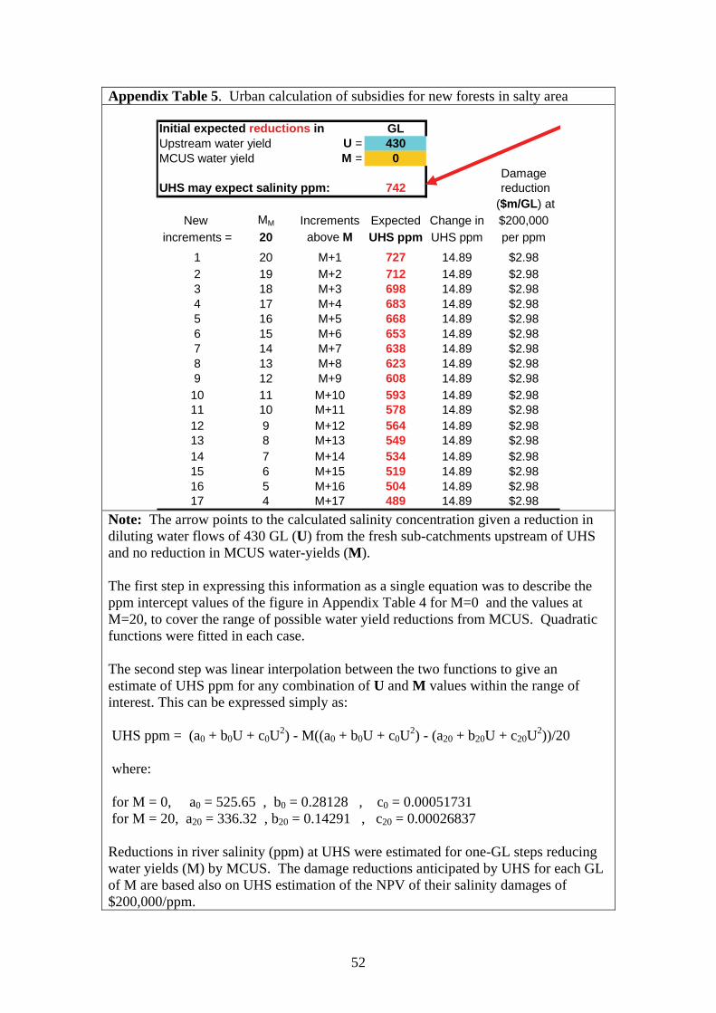
52
Appendix Table 5. Urban calculation of subsidies for new forests in salty area
Initial expected reductions in GLUpstream water yield U = 430MCUS water yield M = 0
DamageUHS may expect salinity ppm: 742 reduction
($m/GL) atNew MM Increments Expected Change in $200,000
increments = 20 above M UHS ppm UHS ppm per ppm
1 20 M+1 727 14.89 $2.982 19 M+2 712 14.89 $2.983 18 M+3 698 14.89 $2.984 17 M+4 683 14.89 $2.985 16 M+5 668 14.89 $2.986 15 M+6 653 14.89 $2.987 14 M+7 638 14.89 $2.988 13 M+8 623 14.89 $2.989 12 M+9 608 14.89 $2.9810 11 M+10 593 14.89 $2.9811 10 M+11 578 14.89 $2.9812 9 M+12 564 14.89 $2.9813 8 M+13 549 14.89 $2.9814 7 M+14 534 14.89 $2.9815 6 M+15 519 14.89 $2.9816 5 M+16 504 14.89 $2.9817 4 M+17 489 14.89 $2.98
Note: The arrow points to the calculated salinity concentration given a reduction in diluting water flows of 430 GL (U) from the fresh sub-catchments upstream of UHS and no reduction in MCUS water-yields (M). The first step in expressing this information as a single equation was to describe the ppm intercept values of the figure in Appendix Table 4 for M=0 and the values at M=20, to cover the range of possible water yield reductions from MCUS. Quadratic functions were fitted in each case. The second step was linear interpolation between the two functions to give an estimate of UHS ppm for any combination of U and M values within the range of interest. This can be expressed simply as: UHS ppm = (a0 + b0U + c0U2) - M((a0 + b0U + c0U2) - (a20 + b20U + c20U2))/20 where: for M = 0, a0 = 525.65 , b0 = 0.28128 , c0 = 0.00051731 for M = 20, a20 = 336.32 , b20 = 0.14291 , c20 = 0.00026837 Reductions in river salinity (ppm) at UHS were estimated for one-GL steps reducing water yields (M) by MCUS. The damage reductions anticipated by UHS for each GL of M are based also on UHS estimation of the NPV of their salinity damages of $200,000/ppm.

53
Appendix Table 6. CAVEATS (warnings and what research remains to be done, or done better)
“The aim of science is to seek the simplest explanations of complex facts. We are apt to fall into the error of thinking that the facts are simple because simplicity is the goal of our quest. The guiding motto in the life of every natural philosopher should be, Seek simplicity and distrust it.” Alfred North Whitehead (1919)
1. This study presents static, deterministic models rather than stochastic (probabilistic) analyses. Possessing the virtue of simplicity, they do not account for year to year variations in prices or rainfall, or sustained drought periods.
2. The study takes the simplifying assumption that all downstream water
entitlements, high and general security, are the same and fully deliverable, expressing rights to exact volumes of water to the entitlement holder each year and tradable as such. Where there has been over-allocation of water entitlements or shortfalls in rain, however, general security allocations will only be some fraction of the face value of the entitlements. These fractions have been reduced to zero or near zero in drought periods. Reconciliation of these issues is a subject worthy of further study.
3. To permit the planting of a new forest area that will use 1 GL of extra water in
a normal year, for example, the purchase of a permanent general security entitlement to one GL, which may be expected to deliver only, say, 1/2 GL of water in a normal year, will result in losses to those not selling entitlements. If there were an ‘exchange rate’ that would equate some number of general security entitlements to one high security entitlement, a rule permitting new forest plantations could be made to reflect this. That is, the extra water new forests consume beyond the previous land uses may be considered to be the equivalent of high security water consumption.
4. Although sale of downstream water entitlements may just balance reductions
in river flow due to new tree plantations, water delivery efficiency may be reduced and overhead costs increased for those not selling entitlements. Our analysis has not counted these costs, which are worthy of further study.
5. There is no doubt that general security water entitlements, which receive only
allocated shares of their denominated volumes according to the rainfall and storage levels that differ from year to year, will present results varying from those shown. Probabilistic volumes of water may be reconciled using ‘state contingent’ analysis. The present study provides many of the details that would allow such analysis.
6. The study takes the simplifying assumption that ‘off allocation’ flows from
unregulated rivers (such as the Bell, Talbragar and Little River) are subject to marketable entitlements, though in reality they are not. Indeed, irrigators may be allowed to pump river water for a 24 hour period following short-notice announcements from the water authority. Also, tactical releases of stored water on the backs of the occasional ‘floods’ from the unregulated rivers may be staged by the water authority for the purpose of meeting environmental aims, such as sustaining the Macquarie Marshes.

54
7. Though the Macquarie River is technically classed as non-terminal, the study
ignores any spill-over of water contributing to the larger Murray-Darling Basin. In recent years little water has exited the catchment due to lack of rain and floods; the latter have largely been minimised by dams and water use by irrigators. The study simply assumes long-run average flows of 1975–95 as its base line and does not account for the recent drought period.
8. The study assumes trading is only for permanent, not temporary, water
entitlements though the latter are more common in practice. Such trades are compatible among participants in the current market. However, the question arises of whether new forest plantations might be permitted with purchases of temporary water entitlements when the life of a plantation may run to 30 years. There is a corollary question of re-sale of water entitlements obtained for a forest plantation when the forest is harvested and the land returned to use as pasture.
9. For the sake of simplicity, the study poses an arbitrary high price for any water
entitlements lost by the Wetlands in the cases where new forest plantations do not require water entitlements. Ignored was recent work by Morrison et al. (1999), Bennett (2002) and others on the estimation of monetary values for environmental benefits and costs. Combining the insights and quantitative measures from that research would add depth to the present line of study.
10. We have ignored the fact that it is not simply the annual volume of water, but
the timing of water delivery that affects the wetland environments. For example, pulses of water mimicking floods may be preferred to a continuous seep summing to the same volume over time. This study has not quantified the environmental impacts of changed flows to the Marshes. This remains a serious challenge generally, not just in this case (NRC 2005), a challenge requiring the combined skills of ecologists and resource economists.
11. We have developed the means to define menus of minimum-cost land use
change to deliver different options of water yield and salt loads from a catchment. Can we develop a similar menu of options for a wetland’s response to receiving water in different amounts at different timings? What is the range of options for sustaining a wetland’s biodiversity and its functions, from full and guaranteed to irrecoverable collapse? Some may regard such questions as immoral, in favour of returning to full pre-European settlement conditions at any cost, but these questions must be faced to help assure the future of the most treasured environmental assets.
This long list of caveats covers only some of the great complexities found in the environment and management of a catchment.
55
NSW Department of Primary Industries Economic Research Report Series
All available at http://www.dpi.nsw.gov.au/research/areas/biosecurity/economics-research/reports
Number 1 Brennan, J.P. and Bantilan, M.C.S. 1999, Impact of ICRISAT Research on
Australian Agriculture, Report prepared for Australian Centre for International Agricultural Research, Economic Research Report No. 1, NSW Agriculture, Wagga Wagga.
2 Davies, B.L., Alford, A. and Hollis, G. 1999, Analysis of ABARE Dairy Data
for Six Regions in NSW 1991-92 to 1996-97, Economic Research Report No 2, NSW Agriculture, C.B. Alexander College, Paterson.
3 Brennan, J.P. and Singh, R.P. 2000, Economic Assessment of Improving
Nutritional Characteristics of Feed Grains, Report prepared for Grains Research and Development Corporation, Economic Research Report No. 3, Wagga Wagga.
4 Zhao. X., Mullen, J.D., Griffith, G.R., Griffiths, W.E. and Piggott, R.R. 2000,
An Equilibrium Displacement Model of the Australian Beef Industry, Economic Research Report No 4, NSW Agriculture, Armidale.
5 Griffith, G., I’Anson, K., Hill, D., Lubett, R. and Vere, D. 2001. Previous
Demand Elasticity Estimates for Australian Meat Products, Economic Research Report No 5, NSW Agriculture, Armidale.
6 Griffith, G., I’Anson, K., Hill, D. and Vere, D. 2001. Previous Supply Elasticity
Estimates for Australian Broadacre Agriculture, Economic Research Report No 6, NSW Agriculture, Armidale.
7 Patton, D.A. and Mullen, J.D. 2001, Farming Systems in the Central West of
NSW: An Economic Analysis, Economic Research Report No. 7, NSW Agriculture, Trangie.
8 Brennan, J.P. and Bialowas, A. 2001, Changes in Characteristics of NSW Wheat
Varieties, 1965-1997, Economic Research Report No. 8, NSW Agriculture, Wagga Wagga.
9 Mullen, J.D. 2001, An Economic Perspective on Land Degradation Issues,
Economic Research Report No. 9, NSW Agriculture, Orange. 10 Singh, R.P., Mullen, J.D., and Jayasuriya, R. 2005, Farming Systems in the
Murrumbidgee Irrigation Area in NSW: An Economic Analysis, Economic Research Report No. 10, NSW Department of Primary Industries, Yanco.
11 Brennan, J.P., Aw-Hassan, A., Quade, K.J. and Nordblom, T.L. 2002, Impact of
ICARDA Research on Australian Agriculture, Economic Research Report No. 11, NSW Agriculture, Wagga Wagga.

56
12 Alford, A., Griffith, G. and Davies, L. 2003, Livestock Farming Systems in the Northern Tablelands of NSW: An Economic Analysis, Economic Research Report No. 12, NSW Agriculture, Armidale.
13 Alford, A., Griffith, G. and Cacho, O. 2003, A Northern Tablelands Whole-
Farm Linear Program for Economic Evaluation of New Technologies at the Farm Level, Economic Research Report No. 13, NSW Agriculture, Armidale.
14 Mullen, J.D. and Vere, D.T. 2003, Research and Extension Capabilities -
Program Economists in New South Wales Agriculture, Economic Research Report No. 14, NSW Agriculture, Orange.
15 Farquharson, R.J., Griffith, G.R., Barwick, S.A., Banks, R.G. and Holmes, W.E.
2003, Estimating the Returns from Past Investment into Beef Cattle Genetic Technologies in Australia, Economic Research Report No. 15, NSW Agriculture, Armidale.
16 O'Donnell, C.J., Griffith, G.R., Nightingale, J.J. and Piggott, R.R. 2004, Testing
for Market Power in Multiple-Input, Multiple-Output Industries: The Australian Grains and Oilseeds Industries, Technical Report for the Rural Industries Research and Development Corporation, Economic Research Report No. 16, NSW Agriculture, Armidale.
17 Brennan, J.P., Martin, P.J. and Mullen, J.D. 2004, An Assessment of the
Economic, Environmental and Social Impacts of NSW Agriculture’s Wheat Breeding Program, Economic Research Report No. 17, NSW Agriculture, Wagga Wagga.
18 Griffith, G.R., Davies, B.L., Alford, A.R., Herd, R.M., Parnell, P.F. and
Hegarty, R.S. 2004, An Assessment of the Economic, Environmental and Social Impacts of NSW Agriculture’s Investment in the Net Feed Efficiency R,D&E Cluster, Economic Research Report No. 18, NSW Department of Primary Industries, Armidale.
19 Scott, J.F. and Farquharson, R.J. 2004, An Assessment of the Economic Impacts
of NSW Agriculture’s Research and Extension: Conservation Farming and Reduced Tillage in Northern NSW, Economic Research Report No. 19, NSW Department of Primary Industries, Tamworth.
20 Scott, J.F., Farquharson, R.J. and Mullen, J.D. 2004, Farming Systems in the
Northern Cropping Region of NSW: An Economic Analysis, Economic Research Report No. 20, NSW Department of Primary Industries, Tamworth.
21 Crean, J., Shaw, A., Singh. R. and Mullen, J.D. 2004, An Assessment of the
Economic, Environmental and Social Impacts of NSW Agriculture’s Advisory Programs in Water Use Efficiency, Economic Research Report No. 21, NSW Department of Primary Industries, Orange.
22 Mullen, J.D. 2004, Evaluations in 2003 of Five Areas of Investment by NSW
Agriculture: Summary, Economic Research Report No. 22, NSW Department of Primary Industries, Orange.

57
23 Vere, D.T., Jones, R.E. and Dowling, P.M. 2004, An Economic Evaluation of
Research into the Improved Management of the Annual Grass Weed Vulpia in Temperate Pastures in South-Eastern Australia, Economic Research Report No. 23, NSW Department of Primary Industries, Orange.
24 Jones, R.E. and Dowling, P.M. 2004, Sustainability, Externalities and
Economics: The Case of Temperate Perennial Grazing Systems in NSW, Economic Research Report No. 24, NSW Department of Primary Industries, Orange.
25 Brennan, J.P. and Quade, K.J. 2004, Analysis of the Impact of CIMMYT
Research on the Australian Wheat Industry, Economic Research Report No. 25, NSW Department of Primary Industries, Wagga Wagga.
26 Brennan, J.P., Sykes, J.D. and Scott, J.F. 2005, Trends in Pulse and Oilseed
Crops in Winter Cereal Rotations in NSW, Economic Research Report No. 26, NSW Department of Primary Industries, Wagga Wagga.
27 Vere, D.T., Griffith, G.R. and Silvester, L. 2005, Australian Sheep Industry
CRC: Economic Evaluations of Scientific Research Programs, Economic Research Report No. 27, NSW Department of Primary Industries, Orange.
28 Singh, R.P., Brennan, J.P. Lacy, J. and Steel, F. 2005, An Assessment of the
Economic, Environmental and Social Impacts of the Ricecheck Program, Economic Research Report No. 28, NSW Department of Primary Industries, Yanco.
29 Jones, R., Saunders, G. and Balogh, S. 2005, An Economic Evaluation of a Pest
Management Control Program: “Outfox the Fox”, Economic Research Report No. 29, NSW Department of Primary Industries, Orange.
30 Griffith, G.R., Parnell, P.F. and McKiernan, W. 2005, An Evaluation of the
Economic Benefits to NSW from Investment in the CRC for Beef Genetics Technologies, Economic Research Report No. 30, NSW Department of Primary Industries, Orange.
31 Khairo, S.A., Mullen, J.D., Hacker, R.B. and Patton, D.P 2006, Farming
Systems in the Western Division of NSW: An economic Analysis, Economic Research Report No. 31, NSW Department of Primary Industries, Trangie.
32 Griffith, G., Vere, D., and Jones, R. 2006, Sheep CRC Renewal
Proposal:Economic Evaluation of the Proposed Scientific Themes, Economic Research Report No. 32, NSW Department of Primary Industries, Armidale.
33 Alford, A.R., Cafe, L.M., Greenwood, P.L. and Griffith, G.R. 2007, The
Economic Effects of Early-Life Nutrition in Crossbred Cattle Bred on the NSW North Coast, Economic Research Report No. 33, NSW Department of Primary Industries, Armidale.
34 Jones, R. and Aluwihare, P. 2007, A bioeconomic model for measuring the
opportunity costs of water sharing plans in unregulated river systems: the
58
Mooki river catchment, Economic Research Report No. 34, NSW Department of Primary Industries, Orange.
35 Davies, B.L., Carberry, P.M., Graham, R.P., Mullen, J.D. and Meaker, G.P.,
(2007) StockPlan®: A Decision Aid for Management of Livestock During Drought and Other Times, Economic Research Report No. 35, NSW Department of Primary Industries, Paterson.
36 Gibson, T.S., Allan, G.L., File, G., Mullen, J.D., Scott-Orr, H., 2005, ‘Priorities
and Principles for Investment in Aquaculture Research by NSW Department of Primary Industries’, Economic Research Report No. 36, NSW Department of Primary Industries, Orange.
37 Mounter, S., Griffith, G., Piggott, R., Fleming, E. and Zhao, X. (2007),
Composition of the National Sheep Flock and Specification of Equilibrium Prices and Quantities for the Australian Sheep and Wool Industries, 2002-03 to 2004-05, Economic Research Report No. 37, NSW Department of Primary Industries, Armidale, September.
38 Mounter, S., Griffith, G., Piggott, R., Fleming, E. and Zhao, X. (2007), An
Equilibrium Displacement Model of the Australian Sheep and Wool Industries, Economic Research Report No. 38, NSW Department of Primary Industries, Armidale, September.
39 Davies, L., Quinn, H., Della Bosca, A., Griffith, G., Trengove, G. and Alford, A.
(2007), The Economic Effects of Alternate Growth Path and Breed Type Combinations to Meet Beef Market Specifications across Southern Australia, Economic Research Report No. 39, NSW Department of Primary Industries, Armidale, September.
40 Orr, L., McDougall, S. and Mullen, J. (2008), An Evaluation of the Economic,
Environmental and Social Impacts of NSW DPI Investments in IPM Research in Lettuce, Economic Research Report No. 40, NSW Department of Primary Industries, Orange.
41 Orr, L., Stevens, M. and Mullen, J. (2008), An Evaluation of the Economic,
Environmental and Social Impacts of NSW DPI Investments in IPM Research in Invertebrate Rice Pests, Economic Research Report No. 41, NSW Department of Primary Industries, Orange.
42 Alford, A.R., McKiernan, W.A., Cafe, L.M., Greenwood, P.L. and Griffith, G.R.
(2008), The Economic Effects of Using Heterozygotes for a Non-functional Myostatin Mutation within a Commercial Beef Production System, Economic Research Report No. 42, NSW Department of Primary Industries, Armidale, May.
43 Nordblom, T.L., Finlayson, J.D., Hume, I.H., and Kelly, J.A. (2009), Supply and
Demand for Water use by New Forest Plantations: a market to balance increasing upstream water use with downstream community, industry and environmental use? Economic Research Report No 43, NSW Department of Primary Industries, Wagga Wagga.