Supply Chain Network Competition

in

Time-Sensitive Markets

Anna Nagurney1,2, Min Yu3, Jonas Floden2, and Ladimer S. Nagurney4

1Department of Operations and Information Management

Isenberg School of Management

University of Massachusetts, Amherst, Massachusetts 01003

2School of Business, Economics and Law

University of Gothenburg, Gothenburg, Sweden

3Pamplin School of Business Administration

University of Portland

Portland, Oregon 97203

4 Department of Electrical and Computer Engineering

University of Hartford, West Hartford, Connecticut 06117

March 2014; revised May 2014

Transportation Research E 70, (2014), pp 112-127

Abstract: We develop a game theory model for supply chain network competition in time-

sensitive markets in which consumers respond to the average delivery time associated with

the various firms’ products. The firms’ behavior is captured, along with the supply chain

network topologies, with the governing equilibrium concept being that of Nash equilibrium.

We derive the variational inequality formulation of the equilibrium conditions and provide

illustrative examples. We also identify special cases for distinct applications. An algorithm

is proposed, and the framework further illustrated through a case study in which we explore

varying sensitivities to the average time delivery with interesting results.

Keywords: supply chains, logistics, networks, time-based competition, game theory, freight

services, delay tolerant networks, information asymmetry, variational inequalities

1

1. Introduction

Timely deliveries of products are essential not only to consumers but to a company’s

reputation and bottom line. If products are not delivered in a timely manner, as illustrated

by the December 2013 holiday season shipping fiasco in the United States, the unfulfilled

demands may result in a tremendous loss of good will, anger, frustration, economic losses

due to perished and spoiled products, and the potential loss of future business (cf. Ng and

Stevens (2014)). A similar example from Sweden was when Christmas trees were home-

delivered three days after Christmas due to shipping problems (Ullgren (1999)). Logistics

providers commonly face delivery delays. For example, a large freight train operator reports

that 5% of its trains are more than 1 hour delayed (GreenCargo (2014)), causing many

concerns in the industry about unreliable transport and forcing customers to make costly

contingency plans. At the same time, reliability is ranked as one of the most important

factors when selecting transport solutions (cf. Laitila and Westin (2000), Maier et al. (2002),

Vannieuwenhuyse and Gelder (2003), Danielis et al. (2005), and Floden (2010)).

Hence, in supply chain management, the average time from the placement of an order

to a product’s delivery has emerged as a key performance indicator (KPI), signifying how

effective and efficient a supply chain network is and providing a valuable metric as to the

time a product spends in the system. As noted in Ketchen, Jr. et al. (2008), in the 1990s,

the average time to fulfill customer orders was measured in weeks, while today, delivery times

are being measured in days, or, in some cases, in hours.

In the past decade, in order to increase responsiveness, and to enable comparisons across

supply chains, Intel introduced the average delivery time, the Order Fulfillment Lead Time

(OFLT), as a KPI (see Hensley et al. (2012)). In military and defense, the Logistics Man-

agement Institute (cf. Klapper et al. (1999)) refers to this KPI as the Logistics Response

Time (LRT), measured, typically, in days. This supply chain performance measure is one of

the four that has been utilized by the U.S. Department of Defense. Moreover, the average

time for delivery of critical needs supplies, such as water, food, medicines, and even shelter,

in disasters, is also an important performance measure for humanitarian relief chains (cf.

Beamon (2008); see also Sheu (2007) and Nagurney, Masoumi, and Yu (2014)). Finally,

for pharmaceuticals, more responsive time-efficient supply chains can save lives. As noted

in Darabi (2013), the Kenya pharma supply chain improved the average time for sea and

air shipments to clear customs from 21.8 days to 5.7 days, and from 2.5 days to 1.8 days,

respectively, resulting in more timely deliveries of HIV/AIDS drugs to Kenyans. However,

much work still remains globally. The World Bank Logistics Performance Index shows that

the median import lead time is more than 3.5 times longer in low performing countries than

2

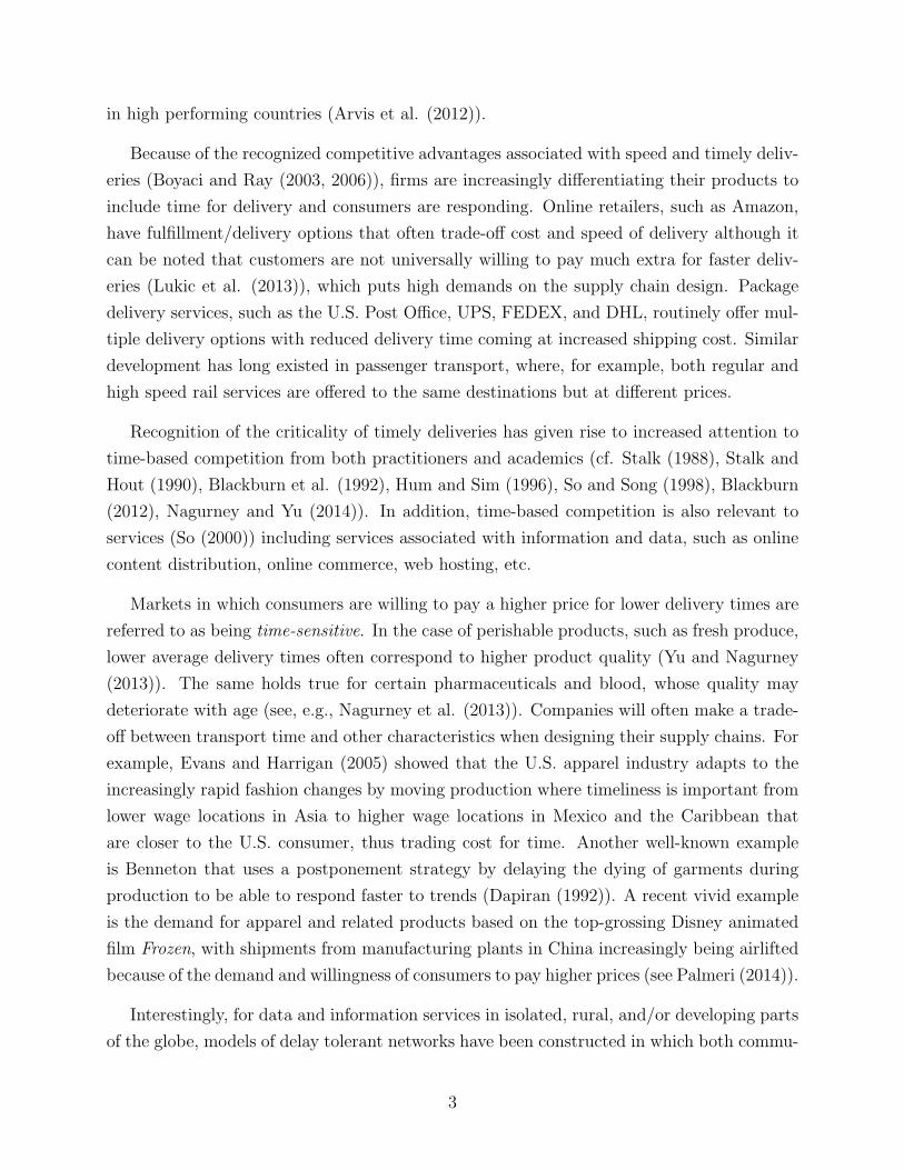
in high performing countries (Arvis et al. (2012)).

Because of the recognized competitive advantages associated with speed and timely deliv-

eries (Boyaci and Ray (2003, 2006)), firms are increasingly differentiating their products to

include time for delivery and consumers are responding. Online retailers, such as Amazon,

have fulfillment/delivery options that often trade-off cost and speed of delivery although it

can be noted that customers are not universally willing to pay much extra for faster deliv-

eries (Lukic et al. (2013)), which puts high demands on the supply chain design. Package

delivery services, such as the U.S. Post Office, UPS, FEDEX, and DHL, routinely offer mul-

tiple delivery options with reduced delivery time coming at increased shipping cost. Similar

development has long existed in passenger transport, where, for example, both regular and

high speed rail services are offered to the same destinations but at different prices.

Recognition of the criticality of timely deliveries has given rise to increased attention to

time-based competition from both practitioners and academics (cf. Stalk (1988), Stalk and

Hout (1990), Blackburn et al. (1992), Hum and Sim (1996), So and Song (1998), Blackburn

(2012), Nagurney and Yu (2014)). In addition, time-based competition is also relevant to

services (So (2000)) including services associated with information and data, such as online

content distribution, online commerce, web hosting, etc.

Markets in which consumers are willing to pay a higher price for lower delivery times are

referred to as being time-sensitive. In the case of perishable products, such as fresh produce,

lower average delivery times often correspond to higher product quality (Yu and Nagurney

(2013)). The same holds true for certain pharmaceuticals and blood, whose quality may

deteriorate with age (see, e.g., Nagurney et al. (2013)). Companies will often make a trade-

off between transport time and other characteristics when designing their supply chains. For

example, Evans and Harrigan (2005) showed that the U.S. apparel industry adapts to the

increasingly rapid fashion changes by moving production where timeliness is important from

lower wage locations in Asia to higher wage locations in Mexico and the Caribbean that

are closer to the U.S. consumer, thus trading cost for time. Another well-known example

is Benneton that uses a postponement strategy by delaying the dying of garments during

production to be able to respond faster to trends (Dapiran (1992)). A recent vivid example

is the demand for apparel and related products based on the top-grossing Disney animated

film Frozen, with shipments from manufacturing plants in China increasingly being airlifted

because of the demand and willingness of consumers to pay higher prices (see Palmeri (2014)).

Interestingly, for data and information services in isolated, rural, and/or developing parts

of the globe, models of delay tolerant networks have been constructed in which both commu-

3

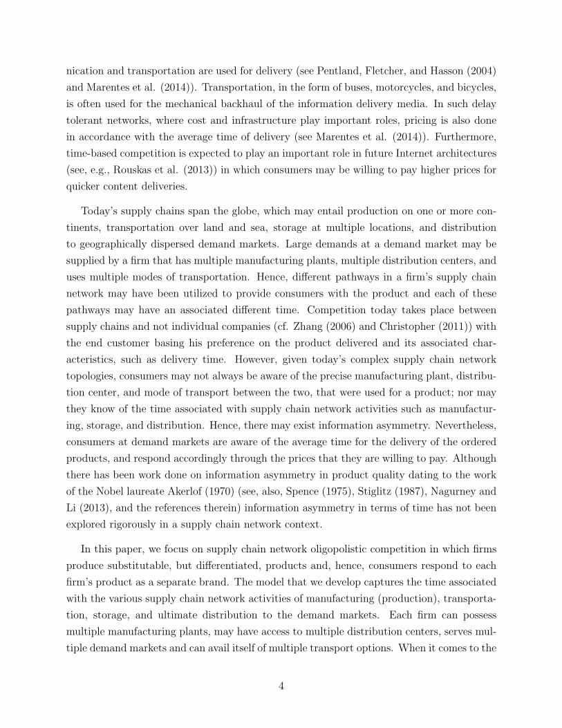
nication and transportation are used for delivery (see Pentland, Fletcher, and Hasson (2004)

and Marentes et al. (2014)). Transportation, in the form of buses, motorcycles, and bicycles,

is often used for the mechanical backhaul of the information delivery media. In such delay

tolerant networks, where cost and infrastructure play important roles, pricing is also done

in accordance with the average time of delivery (see Marentes et al. (2014)). Furthermore,

time-based competition is expected to play an important role in future Internet architectures

(see, e.g., Rouskas et al. (2013)) in which consumers may be willing to pay higher prices for

quicker content deliveries.

Today’s supply chains span the globe, which may entail production on one or more con-

tinents, transportation over land and sea, storage at multiple locations, and distribution

to geographically dispersed demand markets. Large demands at a demand market may be

supplied by a firm that has multiple manufacturing plants, multiple distribution centers, and

uses multiple modes of transportation. Hence, different pathways in a firm’s supply chain

network may have been utilized to provide consumers with the product and each of these

pathways may have an associated different time. Competition today takes place between

supply chains and not individual companies (cf. Zhang (2006) and Christopher (2011)) with

the end customer basing his preference on the product delivered and its associated char-

acteristics, such as delivery time. However, given today’s complex supply chain network

topologies, consumers may not always be aware of the precise manufacturing plant, distribu-

tion center, and mode of transport between the two, that were used for a product; nor may

they know of the time associated with supply chain network activities such as manufactur-

ing, storage, and distribution. Hence, there may exist information asymmetry. Nevertheless,

consumers at demand markets are aware of the average time for the delivery of the ordered

products, and respond accordingly through the prices that they are willing to pay. Although

there has been work done on information asymmetry in product quality dating to the work

of the Nobel laureate Akerlof (1970) (see, also, Spence (1975), Stiglitz (1987), Nagurney and

Li (2013), and the references therein) information asymmetry in terms of time has not been

explored rigorously in a supply chain network context.

In this paper, we focus on supply chain network oligopolistic competition in which firms

produce substitutable, but differentiated, products and, hence, consumers respond to each

firm’s product as a separate brand. The model that we develop captures the time associated

with the various supply chain network activities of manufacturing (production), transporta-

tion, storage, and ultimate distribution to the demand markets. Each firm can possess

multiple manufacturing plants, may have access to multiple distribution centers, serves mul-

tiple demand markets and can avail itself of multiple transport options. When it comes to the

4

latter some may be owned in-house and some may be purchased/contracted for as in the case

of third party logistics providers. The setting depends on the specific application. Hence,

depending on the specific application, the network topology can be adapted accordingly, as

we also demonstrate. The link time consumption functions can depend on the volume of

link flow since it may take longer to produce greater quantities and to ship them (due, for

example, to loading and unloading, etc.); and the same holds for ultimate distribution. Con-

sumers reflect their preferences for the brands through the demand price functions, which,

in general, can depend on the entire demand pattern and on the average times associated

with delivery at the demand markets of all the products. These can also be adapted for

the application of concern. In contrast to the competitive supply chain network model of

Nagurney and Yu (2014), which also made use of link time consumption functions, this new

model is not limited to a single path from a firm to a demand market. Moreover, here we

do not consider time for delivery as a strategic variable in our game theoretic framework

but, rather, as a product characteristic that consumers react to, with the understanding

that the average time is the characteristic (as average quality is in the framework of quality

competition under information asymmetry according to Akerlof (1970)).

We consider the operations of the competing firm’s supply chains through their various

supply chain network activities, which can include production, storage/distribution, as well

as transportation and shipment. We highlight our earlier work on supply chain network

design, which, nonetheless, did not consider time issues (cf. Nagurney and Nagurney (2010),

Nagurney (2010)). It is also worth noting the work of Lin and Chen (2008), who, in contrast,

consider the network design problem for time-definite freight delivery of common carriers, a

third party logistics service provider in supply chains, and propose a generalized hub-and-

spoke network.

The paper is organized as follows. In Section 2, we develop the game theory model for

supply chain network competition in time-sensitive markets in which consumers react to the

average time of delivery associated with the various firms’ products which represent brands.

The behavior of the firms is captured, along with the supply chain network topologies, and

the governing equilibrium concept is that of Nash (1950, 1951) equilibrium. We derive the

variational inequality formulation of the equilibrium conditions and present an existence

result. Examples of industries in which our framework is relevant include food and tobacco

industries in the U.S. as well as vaccine production. For example, Bhuyan and Lopez (1997)

demonstrated empirically that 37 out of 40 food and tobacco manufacturing industries in

the U.S. exhibited substantial oligopoly power. These included such industries as the cereal

preparation industry which ranked at the top of those studied with the highest degree of

5

oligopoly power, with flour and grain, soft drinks, distilled liquor, and pickled sauces also

having high degrees of oligopoly power. The dried fruit and vegetable industries were found

to have the lowest degree of oligopoly power in the same study with such perishable and

time-sensitive food items as poultry, butter, and cheese. Winfree et al. (2004) also identified

oligopoly power in the pear industry, which would fit our framework since fresh fruit is

perishable. Also, as noted by the World Health Organization (2014), since there are very few

manufacturers of vaccines that meet international quality standards, many of the individual

vaccine markets are in the form of oligopolies. Vaccines are clearly another time-sensitive

product (see also Nagurney et al. (2013)) that fits into our framework. Furthermore, we

note that, as noted by Cortez (2012), the fashion and luxury goods market structure is an

oligopoly by nature, with fast fashion (cf. Nagurney and Yu (2012)) representing a time-

sensitive product fitting the supply chain network model developed in this paper.

In Section 3, we provide several illustrative examples. We also identify how this framework

may be used in distinct applications, such as in delay tolerant networks and web hosting.

In Section 4, we propose a computational procedure and further illustrate our framework

through a case study in which we explore varying sensitivities to the average time of delivery

of the products at the demand markets. We find that, as the sensitivity to the average

delivery time at a demand market increases, the firms respond accordingly but at the expense

of decreased profits. Interestingly, we find that the average time for delivery at the other

demand market also decreases, although not as significantly. The case study demonstrates

the usefulness of the theoretical and computational framework. In Section 5, we summarize

our results and present our conclusions.

2. The Supply Chain Network Model for Time-Sensitive Markets

In our framework, the various supply chain activities of each competing firm, which consist

of production, transport/shipment, storage, and distribution of a substitutable but, differ-

entiated, product are represented as links in a supply chain network. The profit-maximizing

firms compete in a noncooperative manner in an oligopolistic fashion to provide their prod-

ucts to the demand markets. The supply chain network economy is represented by all the

firms’ supply chain networks, as depicted in Figure 1. Each of the supply chain activities is

time-consuming and Figure 1 also depicts the progression in time of the various supply chain

activities as a product moves on a path of the network from an origin node, represented

by a firm, to a destination node, represented by a demand market. The firms have perfect

information available as to the product flows on the paths as well as the associated times.

However, the consumers, located at the demand markets, are only aware of the average time

6

for the delivery of the products at the demand markets, and respond to the average time of

receipt of the products through the demand price functions. This information asymmetry is

reasonable since consumers may not have the information (or resources) to track the products

as they proceed through the supply chain network from the origin(s) to the destination(s).

Moreover, they may not even be interested in such specifics.

Li denotes the set of directed links representing the supply chain network economic ac-

tivities associated with firm i; i = 1, . . . , I and G = [N, L] denotes the graph consisting of

the set of nodes N and the set of links L in Figure 1, where L ≡ ∪i=1,...,ILi.

Firm I

Firm 1

��

����

@@

@@@R

��

����

@@

@@@R

����I

����1

...

...

...

...

...

��

��

��

��

��

��

��

��

��

��

��

...

��������

����������*

...

��

��

��

��

��

��

��

��

��

...

ZZ

ZZ

ZZ

ZZ

ZZ

ZZ

ZZ

ZZ

ZZ~

\\

\\

\\

\\

\\

\\

\\

\\

\\

\\

\\

...

HHHHHHHHH

HHHHHHHHH

M I1

����...

����M InI

M

Manufacturing

Transportation

Storage

Distribution

M11

����...

����M1n1

M

-����������

-AAAAAAAAAU

-����������

-AAAAAAAAAU

...

...

...

· · ·

· · ·

· · ·

DI1,1

����...

����DInI

D,1

D11,1

����...

����D1n1

D,1

-

-

-

-

· · ·

· · ·

· · ·

· · ·

DI1,2

����...

����DInI

D,2

D11,2

����...

����D1n1

D,2

����������������������

����������

-���������������

-BBBBBBBBBBBBBBN

AAAAAAAAAU

DDDDDDDDDDDDDDDDDDDDDD

...

...

...

...

...

...

...

...

����RnR

...

R1

����

-

Time T

Figure 1: The Supply Chain Network Topology with Progression in Time

The left-most nodes: i = 1, . . . , I in Figure 1, corresponding to the respective firms,

are connected, via multiple links, to their manufacturing plant nodes, which are denoted,

respectively, by: M i1, . . . ,M

ini

M, and these links represent the manufacturing links. The

7

multiple links reflect different possible manufacturing technologies at the plants and have

associated with them distinct times associated with production as well as distinct total

costs, as we elaborate fully below. The links from the manufacturing plant nodes, in turn,

are connected to the distribution center nodes of each firm i; i = 1, . . . , I, which are denoted

by Di1,1, . . . , D

ini

D,1. These links represent the transportation/shipment links between the

manufacturing plants and the distribution centers where the product is stored. We allow for

different possible modes of transportation, as represented by distinct links, since, in the case

of time-sensitive products, it is important to quantitatively evaluate the impact of different

options in terms of both time and cost. Different modes of transportation may include: rail,

air, truck, ship, as feasible, or intermodal transport. The links joining nodes Di1,1, . . . , D

ini

D,1

with nodes Di1,2, . . . , D

ini

D,2for i = 1, . . . , I correspond to the storage links. The multiple

storage links represent the available storage options. Also, with the storage links there

are associated different times and costs since there may be different options for loading

and unloading the product shipments and inventorying, etc. Finally, there are multiple

possible shipment/distribution links, as mandated by the specific application, joining the

nodes Di1,2, . . . , D

ini

D,2for i = 1, . . . , I with the demand market nodes: R1, . . . , RnR

. Here, we

also allow for multiple modes of transportation, as depicted by the links in Figure 1. Hence,

a firm can allow for multiple delivery options, as reflected by multiple links, to a demand

market, if that is appropriate for the application. We refer to the right-most nodes in Figure

1 as demand markets, noting that they may correspond to retailers, as needed by the specific

application.

In addition, we allow for the possibility that a firm may wish to have the product trans-

ported directly from a manufacturing plant to a demand market, and avail itself of one or

more transportation shipment modes. We can expect that the less time-consuming transport

modes, i.e., the faster ones (such as air), will be more expensive, and that the slower ones

(truck, for example) will be less expensive. These may also represent specific choices such

as express service, next day delivery, and so on. Our general supply chain network topology,

given in Figure 1, can be adapted to include options such as ship transport, depending on

the needs of the decision-maker, and the specific locations of the manufacturing plants, the

distribution centers, as well as the demand markets.

The notation for the model is given in Table 1.

Since the time aspect is the critical feature in our supply chain network competition

model, we first present and discuss the time consumption functions. Each link a, a ∈ L, has

8

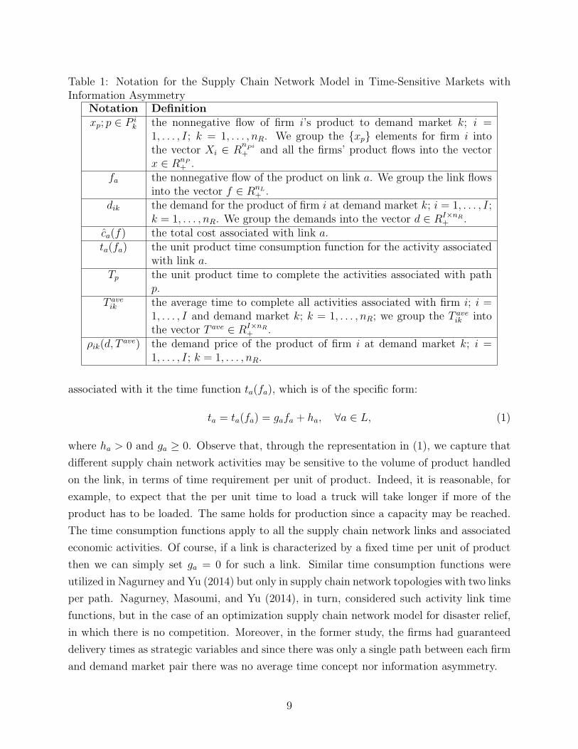
Table 1: Notation for the Supply Chain Network Model in Time-Sensitive Markets withInformation Asymmetry

Notation Definitionxp; p ∈ P i

k the nonnegative flow of firm i’s product to demand market k; i =1, . . . , I; k = 1, . . . , nR. We group the {xp} elements for firm i intothe vector Xi ∈ R

nPi

+ and all the firms’ product flows into the vectorx ∈ RnP

+ .fa the nonnegative flow of the product on link a. We group the link flows

into the vector f ∈ RnL+ .

dik the demand for the product of firm i at demand market k; i = 1, . . . , I;k = 1, . . . , nR. We group the demands into the vector d ∈ RI×nR

+ .ca(f) the total cost associated with link a.ta(fa) the unit product time consumption function for the activity associated

with link a.Tp the unit product time to complete the activities associated with path

p.T ave

ik the average time to complete all activities associated with firm i; i =1, . . . , I and demand market k; k = 1, . . . , nR; we group the T ave

ik intothe vector T ave ∈ RI×nR

+ .ρik(d, T ave) the demand price of the product of firm i at demand market k; i =

1, . . . , I; k = 1, . . . , nR.

associated with it the time function ta(fa), which is of the specific form:

ta = ta(fa) = gafa + ha, ∀a ∈ L, (1)

where ha > 0 and ga ≥ 0. Observe that, through the representation in (1), we capture that

different supply chain network activities may be sensitive to the volume of product handled

on the link, in terms of time requirement per unit of product. Indeed, it is reasonable, for

example, to expect that the per unit time to load a truck will take longer if more of the

product has to be loaded. The same holds for production since a capacity may be reached.

The time consumption functions apply to all the supply chain network links and associated

economic activities. Of course, if a link is characterized by a fixed time per unit of product

then we can simply set ga = 0 for such a link. Similar time consumption functions were

utilized in Nagurney and Yu (2014) but only in supply chain network topologies with two links

per path. Nagurney, Masoumi, and Yu (2014), in turn, considered such activity link time

functions, but in the case of an optimization supply chain network model for disaster relief,

in which there is no competition. Moreover, in the former study, the firms had guaranteed

delivery times as strategic variables and since there was only a single path between each firm

and demand market pair there was no average time concept nor information asymmetry.

9

The unit time on a path p ∈ P ik for a product for i = 1, . . . , I; k = 1, . . . , nR, is then

given by the sum of the link consumption times on links that comprise the path, that is:

Tp =∑a∈L

taδap, ∀p ∈ P ik, ∀i, ∀k, (2)

where δap = 0, if link a is contained in path p, and 0, otherwise.

As mentioned earlier, the consumers at the demand markets reflect their preferences

through the demand price functions, which depend on the average time. Specifically, the

average time T aveik associated with firm i’s product at demand market k is computed by:

T aveik =

∑p∈P i

kTpxp∑

p∈P ikxp

, ∀i, ∀k. (3)

For convenience, we refer to the average time as the average delivery time, with the under-

standing that this time reflects the completion of all the associated activities as represented

by the links that comprise the paths.

We now present the conservation of flow equations and then describe the link total cost

functions and the demand price functions that are used to construct the individual firms’

objective functions and optimization problems.

Specifically, the following conservation of flow equations must hold:∑p∈P i

k

xp = dik, ∀i, ∀k, (4)

since the demand produced by each firm must be satisfied at each demand market. If dik is

equal to zero for any i, k then we simply remove that demand market k from consideration

for firm i and (3) is still well-defined.

Moreover, the path flows must be nonnegative, that is:

xp ≥ 0, ∀p ∈ P. (5)

Furthermore, the expression that relates the link flows to the path flows is given by:

fa =∑p∈P

xpδap, ∀a ∈ L. (6)

In view of (3) and (4), and the demand price functions defined in Table 1, we may

reexpress the demand price functions ρik(d, T ave), as follows:

ρik = ρik(x) ≡ ρik(d, T ave), ∀i, ∀k. (7)

10

We assume that the demand price functions are continuous, continuously differentiable, and

monotone decreasing in both the product demand at the specific demand market and the

average time. Hence, consumers, located at the demand markets, are willing to pay a higher

price for a lower average time of delivery at the demand markets. Similarly, the demand

for a product is higher if the price is lower. Of course, a special case of the demand price

functions is that of ρik = ρik(d, T aveik ), ∀i, k, which implies that consumers at each demand

market are only concerned with the average delivery time of each product at their demand

market.

The total cost on a link, be it a manufacturing/production link, a shipment/distribution

link, or a storage link is assumed, in general, to be a function of the product flows on all the

links, that is,

ca = ca(f), ∀a ∈ L. (8)

The above total cost expressions capture competition among the firms for resources used

in the manufacture, transportation, storage, and distribution of their products. We assume

that the total cost on each link is convex, continuous, and continuously differentiable.

The profit of a firm is the difference between its revenue and its total costs (see, e.g.,

Yu and Nagurney (2013) and the references therein), where the total costs are the total

operational costs in its supply chain network. Here we introduce the novel demand price

functions that capture the average times of delivery applicable to time-sensitive markets.

Hence, the profit function of firm i, denoted by Ui, is given by:

Ui =

nR∑k=1

ρik(d, T ave)dik −∑a∈Li

ca(f). (9)

From (9) we can see that each firm is aware that consumers respond, through the demand

price functions, to the average time of the delivery of the products at the demand markets

but the firms themselves know the times (along with the shipment volumes) of all the paths

in their respective supply chain networks.

Since we are dealing with Cournot-Nash oligopolistic competition, the decision variables

of the firms are their product path flows on their respective supply chain network, with the

path flows also corresponding to their strategies in game theory parlance.Let Xi denote the

vector of path flows associated with firm i; i = 1, . . . , I, where Xi ≡ {{xp}|p ∈ P i}} ∈ RnPi

+ ,

P i ≡ ∪k=1,...,nRP i

k, and nP i denotes the number of paths from firm i to the demand markets.

Thus, X is the vector of all the firms’ strategies, that is, X ≡ {{Xi}|i = 1, . . . , I}.

Through the use of the conservation of flow equations (4), (5), and (6) and the functions

(7) and (8), we define Ui(X) ≡ Ui for all firms i; i = 1, . . . , I, with the I-dimensional vector

11

U consisting of the vector of profits of all the firms:

U = U(X). (10)

In the Cournot-Nash oligopolistic market framework, each firm selects its product path

flows (quantities) in a noncooperative manner, seeking to maximize its own profit, until an

equilibrium is achieved, according to the definition below.

Definition 1: Supply Chain Network Cournot-Nash Equilibrium

A path flow pattern X∗ ∈ K =∏I

i=1 Ki constitutes a supply chain network Cournot-Nash

equilibrium if for each firm i; i = 1, . . . , I:

Ui(X∗i , X∗

i ) ≥ Ui(Xi, X∗i ), ∀Xi ∈ Ki, (11)

where X∗i ≡ (X∗

1 , . . . , X∗i−1, X

∗i+1, . . . , X

∗I ) and Ki ≡ {Xi|Xi ∈ R

nPi

+ }.

Hence, an equilibrium is established if no firm can unilaterally improve its profit by

changing its product flows throughout its supply chain network, given the product flow

decisions of the other firms.

Next, we derive the variational inequality formulations of the Cournot-Nash equilibrium

for the supply chain network with information asymmetry in time-sensitive markets satisfying

Definition 1, in terms of path flows (see Cournot (1838), Nash (1950, 1951), Gabay and

Moulin (1980), Nagurney (2006), and Nagurney et al. (2013)).

Theorem 1

Assume that, for each firm i; i = 1, . . . , I, the profit function Ui(X) is concave with respect

to the variables in Xi, and is continuously differentiable. Then X∗ ∈ K is a supply chain

network Cournot-Nash equilibrium according to Definition 1 if and only if it satisfies the

variational inequality:

−I∑

i=1

〈∇XiUi(X

∗), Xi −X∗i 〉 ≥ 0, ∀X ∈ K, (12)

where 〈·, ·〉 denotes the inner product in the corresponding Euclidean space and ∇XiUi(X)

denotes the gradient of Ui(X) with respect to Xi. Variational inequality (12), in turn, for

our model, is equivalent to the variational inequality in path flows: determine the vector of

equilibrium path flows x∗ ∈ K1 such that:

I∑i=1

nR∑k=1

∑p∈P i

k

∂Cp(x∗)

∂xp

− ρik(x∗)−

nR∑l=1

∂ρil(x∗)

∂xp

∑q∈P i

l

x∗q

× [xp − x∗p] ≥ 0, ∀x ∈ K1, (13)

12

where K1 ≡ {x|x ∈ RnP+ }, and for each path p; p ∈ P i

k; i = 1, . . . , I; k = 1, . . . , nR,

∂Cp(x)

∂xp

≡∑a∈Li

∑b∈Li

∂cb(f)

∂fa

δap. (14)

Proof: See the Appendix.

Variational inequalities (13) can be put into standard form (see Nagurney (1999)): de-

termine X∗ ∈ K such that:

〈F (X∗), X −X∗〉 ≥ 0, ∀X ∈ K, (15)

where 〈·, ·〉 denotes the inner product in n-dimensional Euclidean space. Let X ≡ x and

F (X) ≡[∂Cp(x)

∂xp

− ρik(x)−nR∑l=1

∂ρil(x)

∂xp

∑q∈P i

l

xq;

p ∈ P ik; i = 1, . . . , I; k = 1, . . . , nR

], (16)

and K ≡ K1, then (13) can be re-expressed as (15).

Since the feasible set K1 is not compact, we cannot obtain the existence of a solution

simply based on the assumption of the continuity of F . However, the demand dik for each

firm i’s product; i = 1, . . . , I at every demand market Rk; k = 1, . . . , nR, may be assumed

to be bounded, since the population requiring these products is finite (although it may be

large). Consequently, in light of (3) and (4), we have that:

Kb ≡ {x| 0 ≤ x ≤ b}, (17)

where b > 0 and x ≤ b means that xp ≤ b for all p ∈ P ik; i = 1, . . . , I, and k = 1, . . . , nR.

Then Kb is a bounded, closed, and convex subset of K1. Thus, the following variational

inequality

〈F (Xb), X −Xb〉 ≥ 0, ∀X ∈ Kb, (18)

admits at least one solution Xb ∈ Kb, since Kb is compact and F is continuous. Therefore,

following Kinderlehrer and Stampacchia (1980) (see also Theorem 1.5 in Nagurney (1999)),

we have the following theorem:

13

Theorem 2: Existence

There exists at least one solution to variational inequality (13), since there exists a b > 0,

such that variational inequality (18) admits a solution in Kb with

xb ≤ b. (19)

3. An Illustrative Example and Variants

We now present an illustrative example, along with several variants.

Consider the supply chain network topology given in Figure 2 in which there are two

firms, each of which potentially supplies a single demand market, represented as node R1,

and has, at its disposal, a single manufacturing plant and a single distribution center. The

links are labeled in the figure.

� ��R1

�

JJ

JJJ

8

4

D21,2

� ��

� ��D11,2

-

-

7

3

D21,1

� ��

D11,1� ��

-

-

6

2

M21

� ��

M11� ��

-

-

5

1

� ��2

� ��1

Firm 2

Firm 1

Time T

-

Figure 2: Supply Chain Network Topology for an Illustrative Example and Two Variants

Specifically, Firm 1 is based in the U.S., and its manufacturing plant M11 is also located

in the U.S., as is its distribution center. Firm 2 is based in Asia, where its manufacturing

plant M21 is located; however, its distribution center is in the U.S. The demand market R1

is located in the U.S. Note that, in Figure 2, links 1 and 5 denote manufacturing links; links

2,4,6, and 8 denote transportation links, with links 3 and 7 corresponding to storage at the

distribution centers.

Because there is only a single path p1 = (1, 2, 3, 4) connecting Firm 1 with demand market

R1 and a single path p2 = (5, 6, 7, 8) connecting Firm 2 with R1 the average time expressions

(cf. (3)) become T ave11 = Tp1 and T ave

21 = Tp2 . The time durations are in terms of days.

14

The demand price functions (cf. Table 1) are as below.

ρ11(d, T ave) = −2d11 − d21 − 3T ave11 + 3T ave

21 + 100, (20)

ρ21(d, T ave) = −3d21 − d11 − 2T ave21 + 2T ave

11 + 100. (21)

These demand price functions, can be reexpressed in path flows, as in (7), and, here,

because of the topology in Figure 2, become:

ρ11(x) = −2xp1 − xp2 − 3Tp1 + 3Tp2 + 100,

ρ21(x) = −3xp2 − xp1 − 2Tp2 + 2Tp1 + 100,

where, in view of the link time unit functions given in Table 1, Tp1 = 3.5xp1 + 14 and

Tp2 = 3.1xp2 + 14.

The remainder of the input data for this example are reported in Table 2.

Table 2: Total Link Operational Cost and Link Unit Time Functions, and Equilibrium LinkFlow Solution for Illustrative Example

Link a ca ta(fa) f ∗a1 5f 2

1 + 10f1 .5f1 + 10 3.312 2f2 f2 + 1 3.313 f 2

3 + f3 f3 + 1 3.314 3f4 f4 + 2 3.315 f 2

5 + 5f5 .1f5 + 4 4.646 8f6 f6 + 7 4.647 f 2

7 + f7 f7 + 1 4.648 2f8 f8 + 2 4.64

Because of the simplicity of the supply chain network topology, the equilibrium path flows,

which induce the equilibrium link flows reported in Table 2, can be computed by solving a

2× 2 system of equations (under the assumption that both paths are used and, hence, have

positive flows), yielding for path p1, x∗p1= 3.31, and for path p2, x∗p2

= 4.64.

The values of the incurred demand market prices at the equilibrium are: ρ11 = 97.10,

ρ21 = 77.20 with the average time values being: T ave11 = Tp1 = 25.59 and T ave

21 = Tp2 = 28.37.

Firm 1 earns a profit of 202.74 whereas Firm 2 earns a profit of 240.79. Hence, Firm 2

compensates for its greater distance from the demand market by lower manufacturing times

as well as lower manufacturing costs.

15

Variant 1

Consider the following variant. Firm 1 has enhanced its manufacturing process, which has

resulted in greater efficiency and time reduction with the consequence that its unit time

function on link 1 has been reduced to: t1(f1) = .5f1 + 5. All other data remain as in Table

2 and the demand price functions remain unchanged.

The new equilibrium path flow pattern is: x∗p1= 3.64 and x∗p2

= 4.28 with the equilibrium

link flow pattern being f ∗1 = f ∗2 = f ∗3 = f ∗4 = 3.64 and f ∗5 = f ∗6 = f ∗7 = f ∗8 = 4.28. The

values of the average times are: T ave11 = Tp1 = 21.72 and T ave

21 = Tp2 = 27.62. Hence, the

demand for Firm 1’s product has increased, since it has reduced its (average) time for the

delivery of its product and that for Firm 2’s product has decreased, due to the competition.

The values of the incurred demand market prices at the equilibrium are now: ρ11 = 105.06,

ρ21 = 72.47. Firm 1 earns a profit of 244.47 whereas Firm 2 earns a profit of 204.91. Hence,

Firm 1’s profit has increased and now surpasses that of Firm 2’s.

Variant 2

In the second variant we kept the data as in Variant 1 but now Firm 1 has reduced its

operational cost associated with the manufacturing link 1 so that ca(f) = 2.5f 21 +10f1, with

the remainder of the data unchanged. The new equilibrium path flow pattern is: x∗p1= 4.25

and x∗p2= 4.44 with the equilibrium link flow pattern being f ∗1 = f ∗2 = f ∗3 = f ∗4 = 4.25

and f ∗5 = f ∗6 = f ∗7 = f ∗8 = 4.44. The values of the average times are: T ave11 = Tp1 = 23.86

and T ave21 = Tp2 = 27.77. Hence, the demand for Firm 1’s product has again increased, even

though its delivery time has increased (slightly). In fact, Firm 1 now has almost the same

size market share as that of Firm 2. The values of the incurred demand market prices at the

equilibrium are now: ρ11 = 98.79 and ρ21 = 74.62. Consumers are increasingly attracted to

Firm 1’s product. Firm 1 earns a profit of 288.40 whereas Firm 2 earns a profit of 220.87.

Firm 1’s profit has further increased, whereas that of Firm 2 has also increased, but not as

significantly.

Variant 3

In the third variant of the Illustrative Example, we assumed that the Asian firm, Firm 2, is

very concerned by the increasing success of Firm 1 and has acquired a second manufacturing

plant, M22 , as depicted in Figure 3, which is located in the U.S. Firm 2 still, however, utilizes

its distribution center in the U.S. and serves the same demand market as before. Also, the

demand price functions remain as in (20) and (21). However, notice that the average time

expression T ave21 does not take on the form Tp2 as in the preceding examples, since now there

16

is another path p3 = (9, 10, 7, 8) available for Firm 2.

The data, for convenience of the reader, are reported in Table 3. The input data are as

for Variant 2 but with new data added for the two new links 9 and 10 in Figure 3. The data

in Table 3 reflect that the Asian firm’s manufacturing plant is now closer to its distribution

center (and its demand market) in the U.S. The equilibrium path flow pattern, is now: for

Firm 1: x∗p1= 4.01 and for Firm 2: x∗p2

= 2.78 and x∗p3= 2.23 with the induced equilibrium

link flow pattern as reported in Table 3. The values of the incurred demand market prices at

the equilibrium are now: ρ11 = 94.18 and ρ21 = 76.13. Firm 1 now earns a profit of 257.21

and Firm 2 a profit of 255.97. The values of the average times are: T ave11 = Tp1 = 23.03 and

T ave21 =

Tp2xp2+Tp3xp3

xp2+xp3= 25.44, where Tp2 = 27.09 and Tp3 = 23.38..

� ��R1

�

JJ

JJJ

8

4

D21,2

� ��

� ��D11,2

-

-

7

3

D21,1

� ��

D11,1� ��

-

-

6

2

M21

� ���

���� @

@@@R

� ��9 10

M22

M11� ��

-

-

5

1

� ��2

� ��1

Firm 2

Firm 1

Time T

-

Figure 3: Supply Chain Network Topology for Variants 3 and 4

Table 3: Total Link Operational Cost and Link Unit Time Functions for Variant 3, andEquilibrium Link Flow Solution

Link a ca ta(fa) f ∗a1 2.5f 2

1 + 10f1 .5f1 + 5 4.012 2f2 f2 + 1 4.013 f 2

3 + f3 f3 + 1 4.014 3f4 f4 + 2 4.015 f 2

5 + 5f5 .1f5 + 4 2.786 8f6 f6 + 7 2.787 f 2

7 + f7 f7 + 1 5.018 2f8 f8 + 2 5.019 3f 2

9 + 10f9 .5f9 + 5 2.2310 2f10 f10 + 2 2.23

17

Firm 2, by adding a new manufacturing plant that is closer to its distribution center and

demand market has reduced its average time and now enjoys higher profit. Firm 1, in turn,

because of the increased competition from Firm 2, now suffers a decrease in profits.

Variant 4

Variant 4 had the same data as Variant 3, with the input data as reported in Table 3,

except that now Firm 2 engages in additional marketing to inform U.S. consumers that it

has invested in a plant in the U.S., with the result that the demand price function for its

product has now been changed from the one in (26) to:

ρ21(d, T ave) = −3d21 − d11 − 2T ave21 + 2T ave

11 + 200. (22)

Hence, the consumers at the demand market are now willing to pay a higher price for

Firm 2’s product.

The equilibrium path flow pattern, is now: for Firm 1: x∗p1= 5.17 and for Firm 2:

x∗p2= 6.24 and x∗p3

= 4.08 with the induced equilibrium link flow pattern given by: f ∗1 =

f ∗2 = f ∗3 = f ∗4 = 5.17, f ∗5 = f ∗6 = 6.24, f ∗7 = f ∗8 = 10.32, and f ∗9 = f ∗10 = 4.08. The

values of the incurred demand market prices at the equilibrium are now: ρ11 = 116.89 and

ρ21 = 138.83. Firm 1 now earns a profit of 428.28 and Firm 2 a profit of 1076.26. The values

of the average times are now: T ave11 = Tp1 = 27.11 and T ave

21 = 39.63 with Tp2 = 41.50 and

Tp3 = 36.76. The demand for Firm 2’s product has more than doubled as compared to the

demand in Variant 3, whereas its profit has more than quadrupled. Interestingly, the profit

for Firm 1 has also increased, by about 60%, demonstrating the impact of one firm’s decision

on the other, which may not be immediately apparent or expected. Hence, the impacts of

competition are revealed through the equilibrium solutions.

3.1 Additional Applications - Delay Tolerant Networks and Web Hosting

Below, we describe additional applications, which can be addressed using the above gen-

eral competitive network model.

As noted in the Introduction, the supply chain network model developed above can also

be used in certain data and information delivery applications, including those in isolated

regions (whether rural and/or underdeveloped) in which there may be inadequate telecom-

munication infrastructure due to costs. In order to capture competition among providers of

such services, we can envision a topology as depicted in Figure 4, which is a special case

of the one in Figure 1, to reflect that each firm has costs associated with the operation of

18

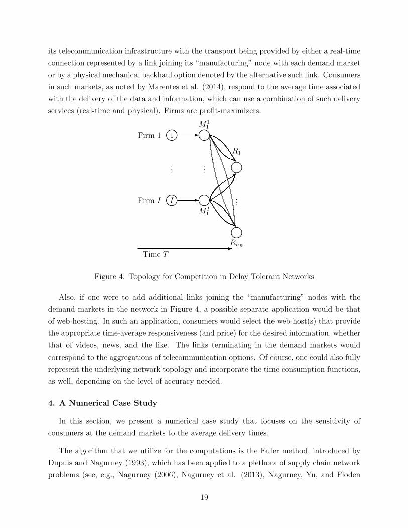
its telecommunication infrastructure with the transport being provided by either a real-time

connection represented by a link joining its “manufacturing” node with each demand market

or by a physical mechanical backhaul option denoted by the alternative such link. Consumers

in such markets, as noted by Marentes et al. (2014), respond to the average time associated

with the delivery of the data and information, which can use a combination of such delivery

services (real-time and physical). Firms are profit-maximizers.

� ��R1

� ��RnR

......

...

R

R

�

M I1

� ��

M11� ��

-

-

� ��I

� ��1

Firm I

Firm 1

-Time T

Figure 4: Topology for Competition in Delay Tolerant Networks

Also, if one were to add additional links joining the “manufacturing” nodes with the

demand markets in the network in Figure 4, a possible separate application would be that

of web-hosting. In such an application, consumers would select the web-host(s) that provide

the appropriate time-average responsiveness (and price) for the desired information, whether

that of videos, news, and the like. The links terminating in the demand markets would

correspond to the aggregations of telecommunication options. Of course, one could also fully

represent the underlying network topology and incorporate the time consumption functions,

as well, depending on the level of accuracy needed.

4. A Numerical Case Study

In this section, we present a numerical case study that focuses on the sensitivity of

consumers at the demand markets to the average delivery times.

The algorithm that we utilize for the computations is the Euler method, introduced by

Dupuis and Nagurney (1993), which has been applied to a plethora of supply chain network

problems (see, e.g., Nagurney (2006), Nagurney et al. (2013), Nagurney, Yu, and Floden

19

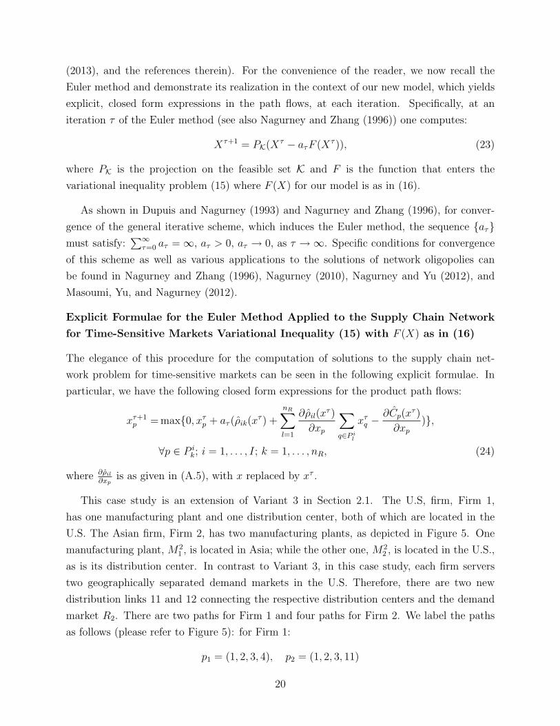
(2013), and the references therein). For the convenience of the reader, we now recall the

Euler method and demonstrate its realization in the context of our new model, which yields

explicit, closed form expressions in the path flows, at each iteration. Specifically, at an

iteration τ of the Euler method (see also Nagurney and Zhang (1996)) one computes:

Xτ+1 = PK(Xτ − aτF (Xτ )), (23)

where PK is the projection on the feasible set K and F is the function that enters the

variational inequality problem (15) where F (X) for our model is as in (16).

As shown in Dupuis and Nagurney (1993) and Nagurney and Zhang (1996), for conver-

gence of the general iterative scheme, which induces the Euler method, the sequence {aτ}must satisfy:

∑∞τ=0 aτ = ∞, aτ > 0, aτ → 0, as τ →∞. Specific conditions for convergence

of this scheme as well as various applications to the solutions of network oligopolies can

be found in Nagurney and Zhang (1996), Nagurney (2010), Nagurney and Yu (2012), and

Masoumi, Yu, and Nagurney (2012).

Explicit Formulae for the Euler Method Applied to the Supply Chain Network

for Time-Sensitive Markets Variational Inequality (15) with F (X) as in (16)

The elegance of this procedure for the computation of solutions to the supply chain net-

work problem for time-sensitive markets can be seen in the following explicit formulae. In

particular, we have the following closed form expressions for the product path flows:

xτ+1p = max{0, xτ

p + aτ (ρik(xτ ) +

nR∑l=1

∂ρil(xτ )

∂xp

∑q∈P i

l

xτq −

∂Cp(xτ )

∂xp

)},

∀p ∈ P ik; i = 1, . . . , I; k = 1, . . . , nR, (24)

where ∂ρil

∂xpis as given in (A.5), with x replaced by xτ .

This case study is an extension of Variant 3 in Section 2.1. The U.S, firm, Firm 1,

has one manufacturing plant and one distribution center, both of which are located in the

U.S. The Asian firm, Firm 2, has two manufacturing plants, as depicted in Figure 5. One

manufacturing plant, M21 , is located in Asia; while the other one, M2

2 , is located in the U.S.,

as is its distribution center. In contrast to Variant 3, in this case study, each firm servers

two geographically separated demand markets in the U.S. Therefore, there are two new

distribution links 11 and 12 connecting the respective distribution centers and the demand

market R2. There are two paths for Firm 1 and four paths for Firm 2. We label the paths

as follows (please refer to Figure 5): for Firm 1:

p1 = (1, 2, 3, 4), p2 = (1, 2, 3, 11)

20

and for Firm 2:

p3 = (5, 6, 7, 8), p4 = (9, 10, 7, 8),

p5 = (5, 6, 7, 12), p6 = (9, 10, 7, 12),

We implemented the Euler method (cf. (24)) for the solution of variational inequality

(13), using Matlab. We set the sequence aτ = .1(1, 12, 1

2, 1

3, 1

3, 1

3, . . .), and the convergence

tolerance was 10−6. In other words, the absolute value of the difference between each path

flow in two consecutive iterations was less than or equal to this tolerance. We initialized the

algorithm by setting the path flows equal to 5.

� ��R1

� ��R2

-�����������

-BBBBBBBBBBN12

4

8

11

D21,2

� ��

� ��D11,2

-

-

7

3

D21,1

� ��

D11,1� ��

-

-

6

2

M21

� ���

���� @

@@@R

� ��9 10

M22

M11� ��

-

-

5

1

� ��2

� ��1

Firm 2

Firm 1

Time T

-

Figure 5: Supply Chain Network Topology for the Case Study

Case Study Example 1

The consumers at demand market R1 are more sensitive to the average delivery times than

those at demand market R2 are. The demand price functions are:

ρ11(d, T ave) = −2d11 − d21 − 3T ave11 + 3T ave

21 + 100,

ρ12(d, T ave) = −3d12 − d22 − 2T ave12 + 2T ave

22 + 100,

ρ21(d, T ave) = −2d21 − d11 − 3T ave21 + 3T ave

11 + 100,

ρ22(d, T ave) = −3d22 − d12 − 2T ave22 + 2T ave

12 + 100.

The link operational cost and link unit time functions are provided in Table 4, along with

the computed equilibrium link flow solution.

21

Table 4: Total Link Operational Cost and Link Unit Time Functions, and Equilibrium LinkFlow Solution for Case Study Example 1

Link a ca ta(fa) f ∗a1 2.5f 2

1 + 10f1 .5f1 + 5 5.062 2f2 f2 + 1 5.063 f 2

3 + f3 f3 + 1 5.064 3f4 f4 + 2 2.335 f 2

5 + 5f5 .1f5 + 4 3.836 8f6 f6 + 7 3.837 f 2

7 + f7 f7 + 1 6.658 2f8 f8 + 2 3.269 3f 2

9 + 10f9 .5f9 + 5 2.8110 2f10 f10 + 2 2.8111 3f11 f11 + 2 2.7312 2f12 f12 + 2 3.39

The equilibrium demands at the demand markets are:

Firm 1: d∗11 = 2.33, d∗12 = 2.73,

Firm 2: d∗21 = 3.26, d∗22 = 3.39.

The average delivery times are:

Firm 1: T ave11 = 23.98, T ave

12 = 24.38,

Firm 2: T ave21 = 24.67, T ave

22 = 28.25.

The incurred demand prices are:

Firm 1: ρ11 = 94.17, ρ12 = 96.17,

Firm 2: ρ21 = 89.06, ρ22 = 79.36.

The profits of Firms 1 and 2 are:

U1 = 311.33, U2 = 372.94.

Since Firm 2 is capable of providing competitive delivery service at a significantly lower

price, Firm 2 dominates both demand markets, leading to a higher profit.

22

Case Study Example 2

This example has the identical data to that of Case Study Example 1 except that the

consumers at demand market R1 are now more sensitive with respect to the average delivery

times. The demand price functions associated with demand market R1 are now:

ρ11(d, T ave) = −2d11 − d21 − 4T ave11 + 4T ave

21 + 100,

ρ21(d, T ave) = −2d21 − d11 − 4T ave21 + 4T ave

11 + 100.

Case Study Example 3

This example has the same data as Case Study Example 1 but now the consumers at the

demand market R1 are even more sensitive with respect to the average delivery times, with

the demand price functions associated with demand market R1 given by:

ρ11(d, T ave) = −2d11 − d21 − 5T ave11 + 5T ave

21 + 100,

ρ21(d, T ave) = −2d21 − d11 − 5T ave21 + 5T ave

11 + 100.

The computed equilibrium demands, average delivery times, prices, and profits for Case

Study Examples 1-3 are reported in Table 5. In Table 6, the computed equilibrium path

flows and the unit time on each path are provided.

A comparison of the results in Case Study Examples 1-3 demonstrates that the average

delivery times from both Firms 1 and 2 to the demand market R1 decline significantly, due

to the consumers’ increased sensitivity to the average delivery times; and both firms charge

higher prices for the timely delivery. It is very interesting to observe that the average delivery

times to demand market R2 also decrease, but slightly. For Firm 2, there are two paths for

each demand market. In order to fulfill the high requirement for timely delivery, Firm 2

mainly relies on its manufacturing plant in the U.S., M22 , to satisfy the demand at demand

market R1; while its Asian manufacturing plant M21 covers all the demand at demand market

R2. The results show that the firms are trading cost for time when reacting to the changed

customer preferences. This is well in line with real world observed behavior, such as for the

perishable products and fashion items discussed in the Introduction.

Moreover, from Table 6, we see that Firm 2’s path p6 is never used at equilibrium in our

three case study examples, and, hence, always has equilibrium flow equal to 0. Also, Firm

2’s equilibrium path flow on its path p3 decreases in Case Study Examples 2 and 3, and

reaches the value of 0 in the latter. The fastest delivery time is achieved by Firm 2 on its

23

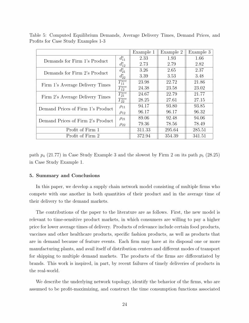
Table 5: Computed Equilibrium Demands, Average Delivery Times, Demand Prices, andProfits for Case Study Examples 1-3

Example 1 Example 2 Example 3

Demands for Firm 1’s Productd∗11 2.33 1.93 1.66d∗12 2.73 2.79 2.82

Demands for Firm 2’s Productd∗21 3.26 2.65 2.37d∗22 3.39 3.53 3.48

Firm 1’s Average Delivery TimesT ave

11 23.98 22.72 21.86T ave

12 24.38 23.58 23.02

Firm 2’s Average Delivery TimesT ave

21 24.67 22.79 21.77T ave

22 28.25 27.61 27.15

Demand Prices of Firm 1’s Productρ11 94.17 93.80 93.85ρ12 96.17 96.17 96.32

Demand Prices of Firm 2’s Productρ21 89.06 92.48 94.06ρ22 79.36 78.56 78.49

Profit of Firm 1 311.33 295.64 285.51Profit of Firm 2 372.94 354.39 341.51

path p4 (21.77) in Case Study Example 3 and the slowest by Firm 2 on its path p5 (28.25)

in Case Study Example 1.

5. Summary and Conclusions

In this paper, we develop a supply chain network model consisting of multiple firms who

compete with one another in both quantities of their product and in the average time of

their delivery to the demand markets.

The contributions of the paper to the literature are as follows. First, the new model is

relevant to time-sensitive product markets, in which consumers are willing to pay a higher

price for lower average times of delivery. Products of relevance include certain food products,

vaccines and other healthcare products, specific fashion products, as well as products that

are in demand because of feature events. Each firm may have at its disposal one or more

manufacturing plants, and avail itself of distribution centers and different modes of transport

for shipping to multiple demand markets. The products of the firms are differentiated by

brands. This work is inspired, in part, by recent failures of timely deliveries of products in

the real-world.

We describe the underlying network topology, identify the behavior of the firms, who are

assumed to be profit-maximizing, and construct the time consumption functions associated

24

Table 6: Computed Equilibrium Path Flows and Path Unit Times for Case Study Examples1-3

Example 1 Example 2 Example 3Firm Manufacturing

PlantDemandMarket

Path x∗p Tp x∗p Tp x∗p Tp

Firm 1M1

1 (in U.S.) R1 p1 2.33 23.98 1.93 22.72 1.66 21.86M1

1 (in U.S.) R2 p2 2.73 24.38 2.79 23.58 2.82 23.02

Firm 2

M21 (in Asia) R1 p3 0.44 28.12 0.01 26.72 0.00 26.04

M22 (in U.S.) R1 p4 2.81 24.13 2.64 22.78 2.37 21.77

M21 (in Asia) R2 p5 3.39 28.25 3.53 27.61 3.48 27.15

M22 (in U.S.) R2 p6 0.00 24.26 0.00 23.67 0.00 22.88

with the various supply chain network activities of manufacturing, transport, storage, and

distribution. In addition, we identify how our general model can also be used to investigate

delay tolerant networks and web-hosting. It also has relevance to time-based competition in

future Internet architectures for content provision.

We utilize variational inequality theory for the formulation of the governing equilibrium

conditions under Cournot-Nash, and also provide qualitative properties of the equilibrium

state. Our proposed computational procedure has nice features for implementation. The

is the first time that such a general model for time-sensitive markets with such a general

network topology has been constructed and formulated.

We provide an illustrative example with variants as well as a numerical case study in which

we report the equilibrium solution, the average times, the individual path times, and the

profits achieved by the firms. The numerical results reveal that the firms are trading cost for

time when reacting to the changed customer preferences. This supports real world observed

behavior for time-sensitive products ranging from fast fashion to perishable products such

as food and vaccines.

The framework also contributes to the literature in terms of managerial insights. For

example, the results imply that, in the case of consumers’ increasing time-sensitivity, it

might be profitable to bring some manufacturing back to the domestic facilities from the

off-shore plants. Our results further support such strategic decision-making in supply chain

management as appropriate location selection for both manufacturing plants and distribution

centers. In addition, the results indicate that, when firms attempt to shorten the average

delivery time to consumers at one time-sensitive demand market, the average delivery time to

the other demand markets may also decrease. This demonstrates synergistic/opportunistic

25

effects that may not have been immediately available without a rigorous computational

framework as we have proposed. This is why it is imperative to capture holistically the

supply chain network activities of firms as well as their interactions using a game theoretic

framework in the context of time-sensitive markets.

Finally, the model contributes to the literature in information asymmetry since the firms

are aware of the product path flows through their supply chains, along with the associated

times, but consumers, located at the demand markets, are only aware of the average time

for their delivery.

Future work may include further disaggregating the supply chain networks of the firms

in order to further detail the production and transportation choices, in the form of routes,

for example. Clearly, supply chain network design for time-sensitive products would also be

of interest.

Acknowledgments

The first author’s research was supported, in part, by the School of Business, Economics and

Law at the University of Gothenburg through its Visiting Professor Program.

This research was also supported, in part, by the National Science Foundation (NSF)

grant CISE #1111276, for the NeTS: Large: Collaborative Research: Network Innovation

Through Choice project awarded to the University of Massachusetts Amherst.

The above support is gratefully acknowledged.

The authors acknowledged the helpful comments and suggestions of three anonymous

reviewers of an earlier version of this paper as well as the comments of the Editor.

References

Akerlof, G.A., 1970. The market for ‘lemons’: Quality uncertainty and the market mecha-

nism. Quarterly Journal of Economics 84(3), 488-500.

Arvis, J.-F., Mustra, M.A., Ojala, L., Shepherd, B., Saslavsky, D., 2012. Connecting to

compete, trade logistics in the global economy, the Logistics Performance Index and its

indicators. The World Bank, Washington DC.

Beamon, B.M., 2008. Performance measurement in humanitarian relief chains. International

Journal of Public Sector Management 21(1), 4-25.

26

Bhuyan, E.R., Lopez, R.A., 1997. Oligopoly power in the food and tobacco industries.

American Journal of Agricultural Economics 79(3), 1035-1043.

Blackburn, J.D., 2012. Valuing time in supply chains: Establishing limits of time-based

competition. Journal of Operations Management 30, 396-405.

Blackburn, J.D., Elrod, T., Lindsley, W.B., Zahorik, A.J., 1992. The strategic value of

response time and product variety. In Manufacturing Strategy: Process and Content, C.A.

Voss, Editor, Chapman and Hall, London, England, pp 261-281.

Boyaci, T., Ray, S., 2003. Product differentiation and capacity cost interaction in time and

price sensitive markets. Manufacturing Service Operations Management 5(1), 18-36.

Boyaci, T., Ray, S., 2006. The impact of capacity costs on product differentiation in delivery

time, delivery reliability, and price. Production and Operations Management 15(2), 179-

197.

Christopher, M., 2011. Logistics and Supply Chain Management: Creating Value-Adding

Networks, 4th ed., Financial Times Prentice Hall, New York.

Cortez, K., 2012. Luxury industry and competitive analysis of ready-to-wear fashion. Uni-

versity of Monaco, Monaco, January 13.

Cournot, A.A., 1838. Researches into the Mathematical Principles of the Theory of Wealth,

English translation, MacMillan, London, England, 1897.

Dafermos, S., Nagurney, A., 1987. Oligopolistic and competitive behavior of spatially sepa-

rated markets. Regional Science and Urban Economics 17, 245-254.

Danielis, R., Marcucci, E., Rotaris, L., 2005. Logistics managers’ stated preferences for

freight service attributes. Transportation Research E 41(3), 201-215.

Dapiran, P., 1992. Benetton – Global logistics in action. International Journal of Physical

Distribution & Logistics Management 22(6), 7-11.

Darabi, T., 2013. To all corners of Kenya. Quality Progress Within Reach, June, 18-25.

Dupuis, P., Nagurney, 1993. Variational inequalities and dynamical systems. Annals of

Operations Research 44, 9-42.

Evans, C., Harrigan, J., 2005. Distance, time, and specialization: Lean retailing in general

27

equilibrium. The American Economic Review 95(1), 292-313.

Floden, J., Barthel, F., Sorkina, E., 2010. Factors influencing transport buyers choice of

transport service - A European literature review. Paper presented at 12th WCTR conference,

Lisbon, Portugal.

Gabay, D., Moulin, H., 1980. On the uniqueness and stability of Nash equilibria in noncoop-

erative games. In Applied Stochastic Control of Econometrics and Management Science, A.

Bensoussan, P. Kleindorfer, C.S. Tapiero, Editors, North-Holland, Amsterdam, The Nether-

lands, pp 271-294.

GreenCargo, 2014. Punktlighet (Puncutality), retreived May 27, 2014

http://www.greencargo.com/sv/Vara-tjanster/Darfor-Green-Cargo/Punktlighet/

Hensley, R., Muthusami, K., Quah, K.C., Wu, J., Zinsli, M., 2012. Transforming Intel’s

supply chain to meet market challenges. Intel IT, IT Best Practices, Supply Chain and

Business Transformation, January.

Hum, S.-H., Sim, H-H., 1996. Time-based competition: Literature review and implications

for modelling. International Journal of Operations and Production Management 16, 75-90.

Ketchen, Jr., D.J., Rebarick, W., Hult, G.T.M., Meyer, D., 2008. Best value supply chains:

A key competitive weapon for the 21st century. Business Horizons 51, 235-243.

Kinderlehrer, D., Stampacchia, G., 1980. An Introduction to Variational Inequalities and

Their Applications. Academic Press, New York.

Klapper, L.S., Hamblin, N., Hutchison, L., Novak, L., Vivar, J., 1999. Supply chain man-

agement: A recommended performance measurement scorecard. Logistics Management In-

stitute, McLean, Virginia.

Laitila, T., Westin, K., 2000. Miljohansyn vid val av godstransportor. Umea University,

Sweden.

Lin, C.-C., Chen, S.-H., 2008. An integral constrained generalized hub-and-spoke network

design problem. Transportation Research E 44(6), 986-1003.

Lukic, V., Souza, R., Wolfgang, M., 2013. Same-day delivery - Not yet ready for prime time,

bcg.perspectives. The Boston Consulting Group, Boston, April.

Maier, G., Bergman, E.M., Lehner, P., 2002. Modelling preferences and stability among

28

transport alternatives. Transportation Research E 38(5), 319-334.

Marentes, L.A., Wolf, T., Nagurney, A., Donosoa, Y., Castro, H., 2014. Overcoming eco-

nomic challenges of Internet operators in low income regions through a delay tolerant archi-

tecture with mechanic backhauls. Universidad de los Andes, Bogota, Colombia.

Masoumi, A.H., Yu, M., Nagurney, A., 2012. A supply chain generalized network oligopoly

model for pharmaceuticals under brand differentiation and perishability. Transportation

Research E 48, 762-780.

Nagurney, A., 1999. Network Economics: A Variational Inequality Approach, second and

revised edition. Kluwer Academic Publishers, Boston, MA.

Nagurney, A., 2006. Supply Chain Network Economics: Dynamics of Prices, Flows, and

Profits. Edward Elgar Publishing, Cheltenham, England.

Nagurney, A., 2010. Supply chain network design under profit maximization and oligopolistic

competition. Transportation Research E 46, 281-294.

Nagurney, A., Li, D., 2013. Equilibria and dynamics of supply chain network competi-

tion with information asymmetry in quality and minimum quality standards. To appear in

Computational Management Science.

Nagurney, A., Masoumi, A.H., Yu, M., 2014. An integrated disaster relief supply chain

network model with time targets and demand uncertainty. In Regional Science Matters:

Studies in Honour of Walter Isard, A. Rose, P. Nijkamp, K. Kourtit, Editors, Springer,

Berlin, Germany, in production.

Nagurney, A., Nagurney, L.S., 2010. Sustainable supply chain network design: A multicri-

teria perspective. International Journal of Sustainable Engineering 3, 189-197.

Nagurney, A., Yu, M., 2012. Sustainable fashion supply chain management under oligopolis-

tic competition and brand differentiation. International Journal of Production Economics

135, 532-540.

Nagurney, A., Yu, M., 2014. A supply chain network game theoretic framework for time-

based competition with transportation costs and product differentiation. In Optimization

in Science and Engineering - In Honor of the 60th Birthday of Panos M. Pardalos, Th. M.

Rassias, C.A. Floudas, S. Butenko, Editors, Springer, New York, pp 381-400.

29

Nagurney, A., Yu, M., Floden, J., 2013. Supply chain network sustainability under compe-

tition and frequencies of activities from production to distribution. Computational Manage-

ment Science 10(4), 397-422.

Nagurney, A., Yu, M., Masoumi, A.H., Nagurney, L.S., 2013. Networks Against Time:

Supply Chain Analytics for Perishable Products. Springer Business + Science Media, New

York.

Nagurney, A., Zhang, D., 1996. Projected Dynamical Systems and Variational Inequalities

with Applications. Kluwer Academic Publishers, Norwell, MA.

Nash, J.F., 1950. Equilibrium points in n-person games. Proceedings of the National

Academy of Sciences USA 36, 48-49.

Nash, J.F., 1951. Noncooperative games. Annals of Mathematics 54, 286-298.

Ng, S., Stevens, L., 2014. A toy lost in the mail is one thing ... Lobsters, medicines among

perishables affected by Christmas shipping snafu. Wall Street Journal, January 2.

Palmeri, C., 2014. Disney’s ‘Frozen’ dress sets off $1,600 frenzy by parents. Bloomberg

News, April 10.

Pentland, A., Fletcher, R., Hasson, A., 2004. DakNet: Rethinking connectivity in developing

nations. Computer, January, 78-83.

Rouskas, G.N., Baldine, I., Calvert, K., Dutta, R., Griffioen, J., Nagurney, A., Wolf, T., 2013.

ChoiceNet: Network innovation through choice. In Proceedings of the 17th Conference on

Optical Network Design and Modeling (ONDM 2013), April 16-19, 2013, Brest, France.

Sheu, J.-B., 2007. An emergency logistics distribution approach for quick response to urgent

relief demand in disasters. Transportation Research E 43(6), 687-709.

So, K.C., 2000. Price and time competition for service delivery. Manufacturing and Service

Operations Management 2, 392-409.

So, K.C., Song, J.-S., 1998. Price, delivery time guarantees and capacity selection. European

Journal of Operational Research 111, 28-49.

Spence, M., 1975. Monopoly, quality, and regulation. The Bell Journal of Economics 6(2),

417-429.

30

Stalk, Jr., G., 1988. Time – The next source of competitive advantage. Harvard Business

Review 66(4), 41-51.

Stalk, Jr., G., Hout, T.M., 1990. Competing against time: How time-based competition is

reshaping global markets. Free Press, New York.

Stiglitz, J.E., 1987. The causes and consequences of the dependence of quality on price.

Journal of Economic Literature 25(1), 1-48.

Ullgren, S., 1999. Problem med granar pa natet (Problems with on-line Christmas trees).

Goteborgs Posten, December 28.

Vannieuwenhuyse, B., Gelders, L., Pintelon, L., 2003. An online decision support system for

transportation mode choice. Logistics Information Management 16(3), 125-133.

Winfree J.A., McCluskey, J.J., Mittelhammer, R.C., Gutman, P., Seasonal oligopoly power

in the D’Anjou pear industry. Journal of Food Distribution 35(2), 56-65.

World Health Organization, 2014. Global vaccine supply. retrieved May 23, 2014.

http://www.who.int/immunization/programmes systems/procurement/market/global supply/en/

Yu, M., Nagurney, A., 2013. Competitive food supply chain networks with application to

fresh produce. European Journal of Operational Research 224(2), 273-282.

Zhang, D., 2006. A network economic model for supply chain versus supply chain competi-

tion. Omega 34, 283-295.

31

Appendix

Proof of Theorem 1: Variational inequality (12) follows directly from Gabay and Moulin

(1980); see also Dafermos and Nagurney (1987). In view of (4) and (7), we may rewrite the

profit functions as follows: for each firm i, ∀i,

Ui(X) ≡ Ui =

nR∑l=1

ρil(x)∑q∈P i

l

xq −∑b∈Li

cb(f). (A.1)

Observe now that

∇XiUi(X) =

[∂Ui

∂xp

; p ∈ P ik; k = 1, . . . , nR

], (A.2)

where for each path p; p ∈ P ik,

∂Ui

∂xp

=∂

[∑nR

l=1 ρil(x)∑

q∈P ilxq −

∑b∈Li cb(f)

]∂xp

=

nR∑l=1

∂[ρil(x)

∑q∈P i

lxq

]∂xp

−∑b∈Li

∂cb(f)

∂xp

= ρik(x) +

nR∑l=1

∂ρil(x)

∂xp

∑q∈P i

l

xq −∑a∈Li

∑b∈Li

∂cb(f)

∂fa

∂fa

∂xp

= ρik(x) +

nR∑l=1

∂ρil(x)

∂xp

∑q∈P i

l

xq −∑a∈Li

∑b∈Li

∂cb(f)

∂fa

δap. (A.3)

In view of (1), (2) and (6), the average time associated with firm i’s product at demand

market k can be rewritten as a function of path flows:

T aveik =

∑q∈P i

k

∑a∈Li

[ga

(∑o∈P i xoδao

)+ ha

]δaqxq∑

q∈P ikxq

, ∀i, ∀k. (A.4)

32

Also, for completeness, according to the chain rule, the partial derivative ∂ρil(x)∂xp

can be expanded as follows: for each path p;

p ∈ P ik,

∂ρil(x)

∂xp

=∂ρil(d, T ave)

∂xp

=

nR∑j=1

∂ρil(d, T ave)

∂dij

∂dij

∂xp

+

nR∑j=1

∂ρil(d, T ave)

∂T aveij

∂T aveij

∂xp

=∂ρil(d, T ave)

∂dik

∂dik

∂xp

+∂ρil(d, T ave)

∂T aveik

∂T aveik

∂xp

+∑j 6=k

∂ρil(d, T ave)

∂T aveij

∂T aveij

∂xp

=∂ρil(d, T ave)

∂dik

+∂ρil(d, T ave)

∂T aveik

[∑a∈Li

(ga

∑o∈P i xoδao + ha

)δap +

∑q∈P i

k

∑a∈Li gaxqδaqδap

] [∑q∈P i

kxq

]−

∑q∈P i

k

∑a∈Li

(ga

∑o∈P i xoδao + ha

)δaqxq[∑

q∈P ikxq

]2

+∑j 6=k

∂ρil(d, T ave)

∂T aveij

∑q∈P i

j

∑a∈Li gaxqδaqδap∑q∈P i

jxq

=∂ρil(d, T ave)

∂dik

+∂ρil(d, T ave)

∂T aveik

[∑a∈Li

(ga

∑o∈P i xoδao + ha

)δap

] [∑q∈P i

kxq

]−

∑q∈P i

k

∑a∈Li

(ga

∑o∈P i xoδao + ha

)δaqxq[∑

q∈P ikxq

]2

+

nR∑j=1

∂ρil(d, T ave)

∂T aveij

∑q∈P i

j

∑a∈Li gaxqδaqδap∑q∈P i

jxq

. (A.5)

By making use of the definition of ∂Cp(x)

∂xpin (14), variational inequality (13) is immediate.2

33