Supply chain cost reduction - Chalmers Publication Library...

Department of Technology Management and Economics Division of Logistics and transportation CHALMERS UNIVERSITY OF TECHNOLOGY Gothenburg, Sweden, 2014 Technical report no. E2014:051

Supply chain cost reduction Manage demand uncertainty in a product repair return flow Master’s thesis in Supply chain management

MARKUS ARTMAN MAX LÖNN SOFIA NILSSON

Technical report no. E2014:051

Supply Chain Cost Reduction - Manage demand uncertainty in a product repair return flow

MARKUS ARTMAN

MAX LÖNN SOFIA NILSSON

Department of Technology Management and Economics Division of Logistics and Transportation

CHALMERS UNIVERSITY OF TECHNOLOGY Gothenburg, Sweden 2014

Supply Chain Cost Reduction - Manage demand uncertainty in a product repair return flow MARKUS ARTMAN MAX LÖNN SOFIA NILSSON Handledare/ Examinator: Mats Johansson Handledare, Wireless Solutions: Joakim Persson © Markus Artman, Max Lönn and Sofia Nilsson, 2014 Technical report no. E2014:051 Department of Technology Management and Economics Division of Logistics and Transportation Chalmers University of Technology SE-412 96 Göteborg Sweden Telephone + 46 (0)31-772 1000 Printed by Chalmers Reproservice Gothenburg, Sweden 2014

I

Supply Chain Cost Reduction - Manage demand uncertainty in a product repair return flow Markus Artman, Max Lönn and Sofia Nilsson Department of Technology Management and Economics Division of Logistics and Transportation Chalmers University of Technology

Abstract Managing an aftermarket supply chain is associated with high levels of complexity. This comes in form of the need to handle extensive number of SKUs over long product lifecycles in relation to highly volatile and uncertain demand. Being cost-efficient in such an environment is challenging since the characteristics of an aftermarket requires high responsiveness to meet customer demand. Wireless Solutions is a world-leading provider of telecommunications equipment and related services to mobile and fixed network operators. Within Wireless Solutions there are three Global Services Logistics Centres (GSLC) where GSLC EMEA works as a support function managing the logistical part in the service contracts of replacing faulty parts with functioning parts towards End Customer. The efficiency of this flow is heavily dependent on the collaboration between the GSLC EMEA and the different Repair Centres that performs the repair service. To generate cost-efficiency there is a need of taking a holistic perspective of the intra-company supply chain in order to not sub-optimise the different actors. This thesis takes a balanced approach departure to investigate the purpose how supply chain costs associated with the WHS Repair Logistics Flow can be reduced by proposing actions to improve the forecasting performance and reducing the intra-monthly variance in the inbound deliveries of faulty parts to Repair Centres. From an initial mapping of the current state there are several problems identified creating a difficult planning environment for all entities. As a starting point it is hard to predict when products need to be replaced due to failure. Additional level of complexity is also generated by the customers’ behaviour. This generates a complex forecast environment creating rippling effect throughout the value chain and affecting the Repair Centres in forms of high deviations between forecast and actual demand. The analysis was conducted on the forecasting management and the possibilities of using a buffer for evening out the variation at the Repair Centres. The analysis profess that the uncertainty within the system drives unnecessary cost in terms of excess capacity for all actors involved. It also concludes that there are measures to be taken to reduce these costs. Regarding forecasting there is a need for increased functional integration as well as an alignment between actors within the system, concerning performance measurements. In addition, increased use of data other than historical demand is recommended, such as installed base data. To reduce the effects of uncertainty for the Repair Centres two distinguished strategies were proposed, both using buffering of faulty units as a levelling mechanism. In the end, a variant of Orders Outside Lead-time was considered the most feasible. By doing so the need for overcapacity to handle variation is reduced. This implies that the costly impact which emerges when less demand than anticipated are received can be diminished. In summary the combination of these measures of improvement creates possibilities for an increased efficiency throughout the supply chain, which would strengthen the value proposition and thereby increasing the competitiveness on the unpredictable aftermarket.

Keywords: aftermarket, demand uncertainty, supply chain, forecasting, levelling

II

Acknowledgement This master thesis has been conducted during the final semester of our master studies within supply chain management. Numerous people have been involved in our thesis and together they have contributed to its fulfilment. We would like to highlight our sincere gratitude towards some specific persons and organisations. To begin with, we would like to thank our company supervisor Joakim Persson for the help and engagement through the learning process. We would also like to thank Mats Johansson for providing a sounding board from an academic perspective. Furthermore we would like to thank Jonas Henriksson and his organisation as well John Ericsson and his organisation for the engagement and highly responsive communication towards us. The GSLC EMEA also deserves a special recognition for providing valuable input and making us feel welcome when visiting. Lastly, but not least, we would like to thank friends, family and loved ones for their enduring support throughout the process.

Gothenburg 8th of June 2014

Markus Artman

Max Lönn

Sofia Nilsson

III

CONTENTS 1 INTRODUCTION ............................................................................................................................ 1

1.1 BACKGROUND ............................................................................................................................. 1 1.2 PROBLEM DESCRIPTION .............................................................................................................. 2 1.3 PURPOSE ...................................................................................................................................... 2 1.4 SCOPE AND LIMITATIONS ............................................................................................................ 2 1.5 THESIS OUTLINE .......................................................................................................................... 3

2 METHODOLOGY ........................................................................................................................... 5 2.1 RESEARCH APPROACH ................................................................................................................ 5 2.2 RESEARCH DESIGN ...................................................................................................................... 7 2.3 DATA COLLECTION ..................................................................................................................... 7 2.4 RESEARCH WORK PROCESS ......................................................................................................... 9 2.5 METHODOLOGY DISCUSSION .................................................................................................... 10

3 FRAME OF REFERENCE ........................................................................................................... 13 3.1 SUPPLY CHAIN MANAGEMENT .................................................................................................. 13 3.2 AFTERMARKET SUPPLY CHAIN ................................................................................................. 13 3.3 SUPPLY CHAIN STRATEGIES ...................................................................................................... 14 3.4 CLASSIFICATION MODELS ......................................................................................................... 18 3.5 FORECASTING ........................................................................................................................... 20 3.6 TOTAL COST CONCEPT .............................................................................................................. 26 3.7 PAST RESEARCH AT WHS DELIVERY ....................................................................................... 29

4 COMPANY DESCRIPTION ........................................................................................................ 31 4.1 WIRELESS SOLUTIONS AB ........................................................................................................ 31 4.2 ORGANISATION ......................................................................................................................... 31 4.3 WHS OPERATIONS AND GSLC EMEA ..................................................................................... 32 4.4 FUNCTIONS WITHIN GSLC ........................................................................................................ 33 4.5 REPAIR CENTRES ...................................................................................................................... 34 4.6 REPAIR SOLUTIONS ................................................................................................................... 34 4.7 PRODUCTS ................................................................................................................................. 35 4.8 WAREHOUSE STRUCTURE ......................................................................................................... 37

5 EMPIRICAL DATA ...................................................................................................................... 39 5.1 VALUE STREAM MAPPING ........................................................................................................ 39 5.2 PERFORMANCE MEASUREMENTS .............................................................................................. 40 5.3 INVENTORY PLANNING .............................................................................................................. 47 5.4 FORECASTING AT GSLC EMEA ............................................................................................... 49 5.5 CONSEQUENCES OF FORECAST DEVIATION ............................................................................... 56 5.6 TOTAL COST ANALYSIS ............................................................................................................ 57

6 ANALYSIS ...................................................................................................................................... 63 6.1 CURRENT STATE ANALYSIS ....................................................................................................... 63 6.2 CHANGING WAYS OF WORKING ................................................................................................ 67 6.3 STRATEGIES FOR REDUCTION OF UNCERTAINY IN INBOUND DELIVERIES ................................ 69 6.4 TOTAL COST ANALYSIS ............................................................................................................. 75 6.5 PLANNING AND FORECASTING .................................................................................................. 78

7 DISCUSSION ................................................................................................................................. 91

IV

7.1 FORECASTING ........................................................................................................................... 91 7.2 STRATEGIES FOR VARIATION REDUCTION ................................................................................ 92 7.3 COMBINATION OF IMPROVEMENT STRATEGIES ........................................................................ 93

8 CONCLUSIONS & RECOMMENDATIONS ............................................................................ 95 8.1 FORECASTING CONCLUSIONS .................................................................................................... 95 8.2 PRODUCTION STRATEGY CONCLUSIONS ................................................................................... 95 8.3 CONCLUDING REMARKS ............................................................................................................ 96 8.4 RECOMMENDATIONS ................................................................................................................. 96

9 REFERENCES ............................................................................................................................... 99

10 APPENDICES ............................................................................................................................ 105 10.1 THROUGHPUT TIME ............................................................................................................... 105

V

ACRONYMS

ADI – Average inter-demand interval BNET – Business unit networks BUGS – Business unit global services CV2 – Square coefficient of variance CU – Customer unit E2E TAT – End-to-end turnaround time EMEA – Europe, Middle East and Africa Region EOL – End of life EFR – Engineering failure rate Faulty stock – Stock of repairable units FIFO – First in first out Good stock – Stock of repaired units GSLC – Global service logistic center ITO – Inventory turnover L2, L3, L4 – Warehouses of different sizes MPE – Mean percentage error MTA – Make to Assembly MTBF – Mean time between failure MTO – Make to Order MTS – Make to Stock NPI – New product introduction OOLT – Orders outside lead-time RMA – Request for material authorization SBA – Syntetos and Boylan approximation SKU – Stock keeping units TAT – Turnaround time VDM – Vendor delivery management

1

1 INTRODUCTION The introduction chapter outlines the foundation of the thesis. Within this chapter the authors present the background of the topic, problem formulation and purpose. In addition, elaboration of the scope and limitations is presented. The end of the chapter presents a disposition of the thesis content, guiding the reader through the main chapters.

1.1 BACKGROUND The aftermarket business environment is often characterised by high levels of profitability and stability in economic downturns. However, managing an aftermarket supply chain is associated with high levels of complexity in terms of long product lifecycles, the number of SKUs handled and the uncertain demand. Being cost-focused in such an environment can be considered challenging due to the complexity and uncertainty it pertains. In today’s dynamic market however, there is a stress among companies to stay competitive by improving efficiency in order to increase profitability (Fahmy et al., 2009).

Wireless Solutions is a world-leading provider of telecommunications equipment and related services to mobile and fixed network operators. The company serves a global dynamic market and is present in over 175 countries. Within Wireless Solutions there are three Global Services Logistics Centres (GSLC) which works as a support function managing the logistical part in the service contracts of replacing faulty parts with functioning parts towards End Customer. The return flow of faulty parts from an End Customer to the GSLCs sent for repair to a Repair Centre and back again to the GSLC is called the WHS Repair Logistics Flow. An overview of the flow is depicted in Figure 1.

Figure 1 – WHS Repair Logistics Flow

Even though visualizing, tracking and managing all entities in the WHS Repair Logistics Flow are complicated activities, the flow is profitable and delivers within the contracted lead-time. However, the setup has been present for some time and optimisation on individual entities has been in focus while more holistically evaluations of alternative setups leading to overall improvements have not been conducted recently.

The efficiency in the WHS Repair Logistics Flow is heavily dependent on the collaboration between the GSLC EMEA and the different Repair Centres. Furthermore, a holistic perspective of the intra-company supply chain for the WHS Repair Logistics Flow is necessary in order to not sub-optimise when improving efficiency for the different actors when conducing this thesis.

2

1.2 PROBLEM DESCRIPTION The uncertain environment of an aftermarket creates difficulties in relation to planning for the GSLC EMEA. It is hard to predict when products will need to be replaced due to failure. Furthermore, customers’ demand behaviour and contracted time to serve, contributes to an even higher level of complexity. From a forecasting point of view this is a challenging environment generating problems when it comes to forecast accuracy. Today the forecasting problem ripples up the supply chain affecting the Repair Centres who perceives a high deviation between the forecasted and the actual volumes that are sent for repair. The problems are present on a monthly level, but are especially prevalent on a weekly basis.

The part of the flow between GSLC and the Repair Centres is solely a make-to-order environment reducing the ability of the Repair Centres to handle the deviation in inbound deliveries compared to forecast. The deviation is today handled through an excessive capacity in terms of both personnel and machinery in order to handle the fluctuations resulting in over-capacity and unnecessary costs. Taking a closer look at the forecasting performance in the WHS Repair Logistics Flow, the accuracy is very low. The actual inbound volumes are allowed to deviate approximately +-20% from the agreed production capacity during a month. However, comparing the previous month’s forecast with the actual volumes, the months with a deviation higher than the agreed level are more than 50%.

1.3 PURPOSE The purpose of this master thesis is to reduce supply chain costs in the WHS Repair Logistics Flow by proposing actions to improve the forecasting performance and reducing the intra-monthly variance in the inbound deliveries of faulty parts to Repair Centres.

1.4 SCOPE AND LIMITATIONS Customer demand can be fulfilled through repair, new buy and reuse. The scope of this report concerns the WHS Repair Logistics Flow, i.e. the fulfilment of customer demand through repair. This flow however includes many intra-firm supply chains, organisations and possible products to use as a foundation for analysis. Delimitations have therefore been made to include two flows; one related to Repair Centre Betamax and one related to Repair Centre Kummle. To fit the initial project assignment the flows should also be handled by the distribution centre in Netherlands.

Repair Centres Betamax, Repair Centre Kummle and the GSLC EMEA in the Netherlands will be explored with primary data gathering methods. End Customers will be excluded and entities between the End Customer and the GSLC EMEA in the Netherlands will solely be analysed with secondary data gathered from statistics of the inbound and outbound flows to and from the L2 distribution centre in Netherlands.

The thesis is conducted from a holistic supply chain perspective. With this said, it is not an intention to provide improvement measures for each individual organisation but rather the supply chain as a whole. Continuously, the suggested improvements should consider the physical infrastructure as of today and not be elaborating on redesigning the current physical settings such as the locations of the Repair Centres or distribution centres in the system.

3

Finally, revenues of the WHS organisation are controlled by service contracts. In reference to the purpose of the thesis focusing on supply chain cost, service contracts to customers will be left constant meaning that the outcome of the project should not alter the End Customer satisfaction or the design of contracts.

1.5 THESIS OUTLINE CHAPTER 2 – METHODOLOGY The methodology chapter describes the research approach and design. Continually it presents the working process to purpose fulfilment. Methods for data collection are outlined and the thesis methodology is elaborated to raise criticism on the performed work.

CHAPTER 3 – FRAME OF REFERENCE The frame of reference presented in this chapter is used in the purpose of generating a solid body of literature. With a spring board on the characteristics of supply chain management on aftermarkets and supply chain strategies, the chapter narrows down into demand classification and ends with presenting forecasting theory and the total cost concept.

CHAPTER 4 – COMPANY DESCRIPTION

The company description presents a thorough description of the company as a whole and the different functions related to the scope of investigation. Furthermore, the chapter also gives an introduction to the product characteristics.

CHAPTER 5 – EMPIRICAL DATA The empirical data chapter gives the reader a basic understanding of the WHS Repair Logistics Flow. The chapter’s point of departure is a value stream map describing the process. After that, the governance structures, the warehouse structure and its planning and forecasting is described. The chapter ends with a total cost mapping of the WHS Repair Logistics Flow.

CHAPTER 6 – ANALYSIS

The analysis chapter firstly gives the reader a general analysis of the current state. Improvement areas are identified related to planning and forecasting. Furthermore improvement strategies for handling the effects of the current situation are elaborated on.

CHAPTER 7 – DISCUSSION

The discussion chapter elaborates on the improvement strategies presented in the analysis chapter. The discussion is surrounding generalizability and barriers for change. Continuously the chapter also address possibilities for combination of the analysed improvement measures.

CHAPTER 8 – CONCLUSIONS AND RECOMMENDATIONS The conclusions and recommendations chapter presents conclusion for the identified improvements of forecasting as well as the change of production strategy. In addition, concluding remarks of integrating the two improvement strategies are elaborated. The chapter continues with an outline of the recommendations to Wireless Solutions for future actions.

5

2 METHODOLOGY The methodology chapter describes the research approach and design. Continually it presents the working process to purpose fulfilment. Methods for data collection are outlined and the thesis methodology is elaborated to raise criticism on the performed work.

2.1 RESEARCH APPROACH The choice of research approach depends on the relationship between theory and research (Kotzab & Westhaus, 2005). According to Kothari (2004) there are two basic approaches to choose from when conducting a research; qualitative and quantitative. Quantitative research optimizes control and generalizability, while qualitative research maximizes realism (Golicic et al., 2005). Continuously, Golicic et al. (2005) explain that these approaches are typically related to the deductive and inductive.

2.1.1 DEDUCTIVE APPROACH

The deductive approach, also called top-down or confirmatory approach (Sachdeva, 2009) goes from a general point of view to the more specific. The hypothesis is formed out of general theory gathering. The goal is then to confirm the hypothesis by using quantitative data collection. Bryman and Bell (2003) express that the research design and the collection of data are guided by specific research questions that derive from theoretical concerns. Bickman and Rog (1998) describe the quantitative approach, typically related to the deductive (Golicic et al., 2005) as a process where the researcher conducts an initial review of appropriate literature, followed by development of a conceptual framework that specifies relevant variables and expected relationships. A deductive approach utilizes quantitative data as a foundation for analysis.

Using a solely deductive approach for this thesis purpose may not be suitable. The rationale behind this is since the context of investigation is partly related to a perceived problem at a specific company and not relied on a theoretical foundation. However, the work is somewhat hypothesis driven in terms of the perceived problems stated by the company, which has had an influence to the investigation. Bryman and Bell (2003) as well as Jacobsen (2002) bring up issues that need to be taken into consideration regarding a deductive approach. Bryman and Bell (2003) state that the relevance of data for specific literature may become apparent only after the empirical data has been collected, meaning that the data may not fit the original hypothesis. This is a risk of doing the thesis in direct relation to the company. During the writing there might be unforeseen paths to follow for further investigation, redirecting the need of data gathering that, as mentioned, not fit the stated hypothesis. Furthermore Jacobsen (2002) states that with this approach there is a risk of missing out important information. This is since the theory gathering might be conducted with expectations of the end result in mind, narrowing the scope of investigation, which is something that the authors would like to avoid by taking a holistic view on the scope of investigation.

2.1.2 INDUCTIVE APPROACH

Instead of the deductive approach, an inductive approach can be chosen. Here the researcher is moving from a specific observation to a broader generalization and theory gathering (Sachdeva, 2009). With this approach the work is initially conducted without any expectations, the hypothesis is based on the observed patterns in the empirical study (Jacobsen, 2002). According to Golicic et al. (2005) the inductive approach is about understanding the phenomenon in its own context. Firstly by collecting

6

data about the everyday experience from the respondent’s perspective, and secondly describing the phenomenon from the respondent’s perspective. The inductive approach utilizes qualitative data gathering to explore the deep structure of the phenomenon using holistic descriptions that explore the multiple dimensions and properties of the phenomenon (Golicic et al., 2005).

The inductive approach is more in line with the way of working for reaching the purpose of the thesis. Since the initial assignment was based on specific perceptions of an underlying problem this approach could have been used for a broader generalization and guidance of theory gathering. However, the perceived problems may have other root-causes than what was initially stated. By focusing on a solely inductive approach there is a perceived risk raised by the authors of not solving the root cause.

2.1.3 BALANCED APPROACH

As seen, the inductive and deductive approach is distinguished from each other. However, choosing one or the other strictly may not be necessary. The choice of approach should be better thought of as a tendency rather than a distinction (Bryman & Bell, 2003). Sachdeva (2009) also supports this aspect and brings arguments on that most social and business researches actually involve both types of reasoning’s throughout the project.

Instead of using one single approach Golicic et al. (2005) elaborate on a balanced approach including both inductive and deductive characteristics for research conducted within a supply chain management context. Golicic et al. (2005) state that the main reason for this approach is due to the complexity of the supply chain environment. They further state that;

“Researchers who exclusively chose one approach seriously delimit the scope of their inquiry and, thereby, their ability to contribute to the body of knowledge”

Golicic et al. (2005) describe that the choice of approach should depend on how much is known about the phenomenon of study, in this case an aftermarket supply chain. If the research focuses on developing an understanding of new or complex phenomena, then it is said that the qualitative approach is typically the best path. If the research however aims to take a more general view in order to explain relationships or demonstrate cause and effect among well-researched concepts, then the broader view provided by the quantitative path is often more appropriate.

Since this research is done for a specific company and in a specified process, it is of high importance to create an initial understanding of the phenomenon of study. Although the authors possess knowledge of the phenomenon from an academic point of view the phenomenon in relation to the specific context is new and unknown. This indicates according to Golicic et al. (2005) choose a qualitative path. However, to be able to provide recommendations related to the context in which the research is done there is also a need of taking a more general view by studying well-researched concepts that could generate insight to fulfilment of the purpose. These issues generate a foundation for this thesis to make a departure in the balanced approach where the combination of inductive and deductive approach will be used for the ability to conduct both quantitative and qualitative data gathering.

7

2.2 RESEARCH DESIGN Case studies involve an examination of a specific phenomenon, a case. It aims to take a small part of a big process and allows that part to represent reality (Ejvegård, 2009). A case can be an individual, a group, an organisation or a situation. As the method is grounded in reality, a holistic perspective can be attained and is suitable for studies of processes and changes (Patel & Davidsson, 2011). The supply chain of investigation is one of many within WHS Repair Logistics Flow. Generalization was required but since the assignment was given on the specific scope, investigating all supply chains was not an option. Therefore, the design of a case study was found most suitable.

A case study is designed differently depending on the situation. It can be single or multiple and can be characterized as holistic or embedded (Yin, 2009). Holistic case studies are characterized by qualitative studies based on narrative a7nd phenomenological descriptions. Emphasis is placed on understanding of the case. Embedded case studies involve more than one unit within the system and are not limited to only qualitative studies (Scholtz & Tietje, 2002).

In relation to the above stated it is possible to argue for several types of approach for the thesis, depending on the definition of the context and unit of analysis. However, since there is a wish to provide a holistic view of the flow between the GSLC and the Repair Centres the definition used in the context is WHS Repair Logistics Flow and the unit of analysis will be the connection towards the two specific Repair Centres.

Figure 2 presents four different setups of a case study design.

Figure 2 - Four different setups for a case study design (Yin, 2009)

2.3 DATA COLLECTION When undertaking a research study there is a need for gathering of information. This information can be regarding a situation, person, problem or phenomenon. The information usually needs to be collected but in some cases it is already available and does only need to be extracted (Kumar, 2011).

8

Based on this statement the source of data may be classified into primary and secondary sources (Krishnaswamy & Satyaprasad, 2010).

2.3.1 PRIMARY DATA COLLECTION

Information that is first-hand collected by the researcher through various information-gathering methods is defined as primary data (Krishnaswamy & Satyaprasad, 2010).

The main method used for primary data collection within this thesis has been interviews. Interviews can be classified into different categories depending on their level of structure (Kumar, 2011). The interviews performed have been of more or less semi-structured character depending on the purpose of the interview. Initially the characteristics of the interviews were open and less controlled i.e. less structured. This was to enable the interview to cover areas and provide information that otherwise might not have been revealed, which is a common aim for the use of semi-structured interviews according to Krishnaswamy and Satyaprasad (2010). Since the initial aim was to get a comprehensive understanding of the phenomenon of study within a context which the authors had little knowledge about, this approach of interviewing was advantageous in terms of data gathering. When better knowledge of the context was developed the need to extract specifically targeted information increased. Therefore, in later stages of the thesis, more structured interviews were applied to the interviews.

Interviews were booked in advance to avoid stressful situations. All interviews were attended by at least two authors to make sure that no information was missed. Further several interviews were recorded. After the interviews, the respondent had the opportunity to review the authors’ notes, to be sure that the information was interpreted correctly. The interviews have mostly been performed face to face with the respondents but also telephone, e-mail and Lync (Internal communications system) have been used.

During the work with the thesis, field studies were also conducted. During these field studies primary data were also collected through observations. The observations aimed to generate visual understanding of the different entities present within the scope of investigation. It also aimed to provide the authors with information on how the information and material handling processes were conducted at the entities of investigation. It also provided visual information of the IT system that is used. A visual experience was helpful to link data gathered in the interviews to the reality when conducting analysis.

2.3.2 SECONDARY DATA COLLECTION

Data collected from secondary sources in contrast to primary is information that has been collected, compiled and published for another purpose, such as academic publications, annual and statistical reports etc. However, in this category of data sources, unpublished material can also be present such as records and registries maintained by firms and organisations (Krishnaswamy & Satyaprasad, 2010).

Within this thesis the secondary data sources have been based on academic papers, annual reports and to a large extent unpublished material in terms of internal documents provided by Wireless Solutions. In addition quantitative data withdrawn from Wireless Solutions ERP system has been used. The main objective for the use of secondary data is to provide a better foundation for scientific generalization and enable verification possibilities for the primary data gathering (Krishnaswamy & Satyaprasad,

9

2010). In accordance with Krishnaswamy and Satyaprasad (2010), the secondary data used in the thesis has the aim to provide foundation to create the body of theory for both the current state and the suggested improvement measures. It has also formed a foundation and guidance for the authors to perform an efficient primary data collection.

The secondary data collection, just as for the primary data, has gone from a more general to a more specific, over the time of the thesis writing. The data gathering for theoretical reference was done by using Summon and Google Scholar as well as Wireless Solutions internal search engine. The first two search engines were used to find academic papers and theoretical literature while the last were used to find internal standard working procedures and process descriptions related to Wireless Solutions. In addition, Chalmers’ library has also been used for gathering of secondary data.

2.4 RESEARCH WORK PROCESS In order to be able to fulfil the purpose of this thesis the work process has gone through four distinguished phases. The work process is an interface between the purpose and the methodology and aims to be decomposed in Figure 3. The figure just presents a schematic outline and it should not be viewed as isolated phases.

Figure 3 - Research work process

2.4.1 PHASE ONE – DEFINING THE RESEARCH FRAMEWORK

Initially the thesis topic was given by a description made by the company, including purpose and background information. Even though this description generates a foundation, elaboration regarding the purpose needs to be conducted to create a framework that practically works for solving the industrial problem within an academic research. Literature reviews and meetings with representatives from both the academic world and the host company were used for elaborating on this matter. Once

10

the purpose and methodological approach were considered aligned by all stakeholders involved, the work of data collection in phase two was started.

2.4.2 PHASE TWO – IDENTIFYING ATTRIBUTES OF THE SYSTEM OF INVESTIGATION

Since the overall aim of this thesis is to propose measures for supply chain cost reduction within the studied system, it was important to firstly break down the purpose into smaller parts. Even though the aim was to solve an industrial problem, there was a need of generating a solid body of theory related to the topic of investigation. This theory included models and definitions that were utilized for establishing an understanding of the supply chain environment in which the units of analysis acted. This phase aimed to generate comprehensive understanding of the current state based on general qualitative data provided by both primary and secondary sources. The findings of phase two acted as a gateway for continuing with the third phase, providing verification of the purpose.

2.4.3 PHASE THREE – INVESTIGATE AND ANALYSE MEASURES OF IMPROVMENT

With the data on hand from the second phase, the third phase continues with deeper exploration on the chosen areas of investigation. Primary data collection was directly targeted toward segmented respondents of interest, concerning the specific areas. Additional secondary data was collected in order to compliment and narrow down literature used in the earlier investigation made in the initial phase. The aim of this phase was to generate description of the relationships between activities and costs and between the activities themselves. This enabled possibilities to observe how changes in one activity affect costs in other activities. The rationale here were that this would help to reduce the risk of sub-optimization by allowing understanding of the changes on the total flow and not on individual activities and cost items in the studied system. Large amount of quantitative data was collected and processed. Simplifications and assumptions were to be made to make the calculations manageable, but the output was to be presented as a ballpark estimation of the supply chain cost reductions for the different changes. The finalizing of the third phase was conducted with an analysis on how the different proposed measures of improvement were to impact the supply chain as a whole in terms of cost saving. This was done by connecting the initial findings in the current state with the proposed measures of improvement. This analysis set the foundation for further discussion.

2.4.4 PHASE FOURE – CONCLUDING FINDINGS AND FINILIZING THE REPORT

The final phase aims to conclude the findings keeping a holistic view of the topic of investigation in relation to the purpose. Findings were to be elaborated with the host company together with finalizing the report.

2.5 METHODOLOGY DISCUSSION Conducting a research means combining input both from the academia and reality. To ensure that these two parameters correlate there is a need to elaborate possible critique towards the methodology used. This is normally done in terms of elaborating around validity and reliability. Validity explores if the research presents what it is stated to present while reliability explores the possibilities of reproducing the study using the same methodology (Kumar, 2011).

Kumar (2011) however argues that these concepts might not be suitable for a research that utilizes qualitative parameters due to its flexibility needed. Since the thesis takes a departure in the balanced

11

approach, quantitative parameters are used in addition to qualitative. Guba (1981) suggests using credibility, transferability, dependability and conformability when elaborating around methodology criticism within these types of research environments.

2.5.1 CREDIBILITY

For a report to have a high credibility the result must be credible and believable from the perspective of the participants in the research (Kumar, 2011). Since the qualitative data handled in a study always can be related to one or more specific sources, these sources is believed to be the best judge on whether their opinions have been reflected in an accurate way.

This thesis mainly contains three types of information sources, both primary and secondary. Firstly the primary data sources in terms of respondents that has been participating and contributing to the data gathering through interviews. Secondly are the authors of the academic papers used in the theoretical reference chapter which is seen as secondary sources. Thirdly are also the authors of the internal Wireless Solutions’ documents, which are secondary data, used as a foundation, together with theory, for primary data gathering.

To ensure credibility among the primary sources, the information gathered and written in the report has been elaborated with the respondents and other representatives at Wireless Solutions. This has been done continuously throughout the writing process as well as with the final report. By giving the respondents the possibility to read and give feedback, inaccurate interpretations have to a large extent been possible to avoid. In addition, most of the interviews have been recorded. This measure has also contributed to decrease the risk of misinterpretation.

The credibility of the secondary sources may be harder to ensure. However, by ensuring the use of latest updated internal document as an information source and also elaborate the finding with employees at the company, credibility in line with what can be considered acceptable is thought to have been reach. Due to the authors’ limited experience, as well as limited access to the ERP system, the collection of quantitative data have had to be trusted to secondary sources. Although the authors specified the needed data, misinterpretations may have occurred affecting the credibility of the quantitative data. Moreover, the authors may not have initially asked for the right data.

Regarding the academic theory used, which is built on secondary sources, credibility has been raised by using more than one source studying the same phenomena. This is in line with what is stated by Jacobsen (2002) as a measure to improve credibility.

2.5.2 TRANSFERABILITY

How well the research can be generalized and transferred into other contexts is measured by the transferability (Kumar, 2011). Single case studies tend to get criticized because one case does not always represent reality in a satisfactory manner (Yin, 2009). Since there has been a single case study performed this affects the transferability and consequently the result cannot be stated to represent all types of Repair Centres within Wireless Solutions. However, by using thorough methodology chapter and in-detailed description of the applied models used, possibilities for others to follow and replicate the result in other contexts are enabled, increasing the transferability. This is a common way of establishing transferability within a research utilizing qualitative parameters (Kumar, 2011). Another issue is that the quantitative data used in the calculations, which also the result is based on, are

12

historical data for 2013. Consequently the result elaborates on historical data and cannot be seen as fully accurate for the future. This creates problems with transferability not only in accordance to what is stated above, between different contexts, but also in relation to transferability in time. The quantitative data used for the calculations it is however somewhat stable looking over a three year period, increasing the transferability.

2.5.3 DEPENDABILITY

Dependability can be seen in how reliable the instrument of measure is and how consistent the use of this instrument has been. Dependability is hard to establish within a research utilizing qualitative parameters. The main reason for this is due to the need of maintaining high flexibility throughout the research (Kumar, 2011). There are two types of instruments used for this thesis; firstly there have been interview guides made before each conducted interview. Though the interviews have been of semi-structured characteristics the template of questions has not always been followed when side tracks of interest have been elaborated. This generates problem for stating a high dependability. There are also occasions where there has only been one respondent answering for a certain topic. This makes reliability of this respondent hard to proof. There is also one issue that might have affected the consistent of instrument use, and thereby the dependability. The fact that the authors have been located at one of the three sites of investigation has made it possible to state questions and ask for input in a non-structural way, causing discussions built on approximation rather than pure facts. To reduce the impact of these non-structural conversations the questions have been raised and clarified at later instances during formal interviews.

The second instrument of use has been computer programs for calculations. The same instrument has been used conducting all calculations. Although the instrument as so is consistently used the methods of handle it may differ, generating incomparable results. This deviation in use of the instrument has been acknowledged at several occasions during the writing of the thesis. This has raised the awareness of the authors and to minimize impact proofing has always been conducted internally.

2.5.4 CONFORMABILITY

The degree to which the result of the thesis can be confirmed by others is stated as conformability (Kumar, 2011). To reach conformability of the thesis stakeholders at both the company and the school have been given the opportunity to review the report. In addition conformability has been established due to the fact that there have been three authors writing the report making it possible to confirm each other’s contributions.

13

3 FRAME OF REFERENCE The frame of reference presented in this chapter is used in the purpose of generating a solid body of literature. With a spring board on the characteristics of supply chain management on aftermarkets and supply chain strategies, the chapter narrows down into demand classification. The chapter ends with presenting forecasting theory and the total cost concept.

3.1 SUPPLY CHAIN MANAGEMENT The shifts in modern business management where individual businesses no longer compete as solely autonomous entities but rather as networks described by Lambert and Cooper (2000), have extended the unit of analysis from individual businesses to the totality of the supply chain (Naim et al., 2002). With a departure in the concept of logistics, the concept of supply chain management widens the scope, seeking to achieve linkage and co-ordination between the processes of other entities in the pipeline, i.e. suppliers and customers, and the organisation itself.

The definition of logistics management, which in turn is part of supply chain management, also highlights the reversed flow i.e. the movement of goods from the traditional end-point in terms of customers back to its place of origin, the manufacturer (Srivastava, 2012). Based on this, it can be assumed that reversed flow, which could be equal to aftermarket supply chain, is part of the supply chain management as well.

3.2 AFTERMARKET SUPPLY CHAIN The interest of managing aftermarket supply chains has grown increasingly (Mollenkopf et al., 2007) for many reasons. One main driver seems to be that management has started to realise the profitability of aftermarket services (Deloitte, 2011) such as repair, maintenance, technical support and spare part sales (Cohen et al., 2006). Glueck et al. (2006) have shown that service operations generate more than 75% higher profitability than overall business operations (Glueck et al., 2006). Cohen et al. (2006) also highlight that the aftermarket has become up to five times larger than the original equipment business.

Other factors that also have had an impact on the development of the aftermarket supply chains are the increased frequency of new product introduction resulting in shorter sales cycles and longer service lifecycles. Continuously, the business of service and spare parts often tends to be far more robust in times of economic downturn. With this foundation the basis of competition is shifting toward the ability to drive business performance through excellence in service and spare parts management (Glueck et al., 2006).

However, despite the potential of the aftermarket supply chain, the reversed supply chain needed for handling spare parts are more complex and harder to manage then the traditional supply chain (Srivastava, 2012). Besides a longer lifecycle, the total number of SKUs is higher than for new products due to the fact that it sometimes includes a lifetime span of assortment. Moreover, the demand for parts and repair services is relatively unstable and difficult to forecast. These issues generate high challenges when it comes to activities such as planning, purchasing, ordering, logistics among others (Deloitte, 2011). The main differences between the supply chains are seen in Figure 4.

14

Figure 4 – Differences between a manufacturing and an after-sales services supply chain (Cohen et al., 2006)

Even though aftermarket and manufacturing supply chains both consist of entities and assets linked by the flow of materials, information and monetary means they differ in many ways. Cohen et al. (2006) suggest that one crucial distinction between the two kinds of supply chains should differentiate the operating philosophies applied to them.

3.3 SUPPLY CHAIN STRATEGIES The purpose of the supply chain strategy is to determine the nature of procurement, transportation of material, manufacturing of products and distribution of the product to the customer (Chopra & Meindl, 2012).

Companies need to classify their products and build strategies in order to fulfil the wanted and expected customer service. Fischer (1997) classifies products into functional and innovative products where the demand characteristics of a spare part align with the demand characteristics of innovative products. The volatile demand and short lead-time requirements are two aspects, but also the high margins and variety. Just as Fisher (1997) argues for a clear distinction between the management of functional and innovative products when it comes to supply chain strategy applied, Cohen et al. (2006) suggest that there is a need to differentiate the operating philosophies applied to a supply chain managing spare parts and a supply chain managing new production. However, there might be aftermarket supply chains that hold products with both innovative and functional characteristics. This implies that to distinguish the strategy there is a need to first look at what type of context the actual supply chain works in; if it is a manufacturing or aftermarket environment. Then secondly establish what type of product and demand characteristics it handles. The different supply chain strategies based on product characteristics are seen in Figure 5.

Figure 5 – Supply Chain strategies based on product characteristics (authors’ illustration based on Fisher, 1997 and

Cohen et al., 2006)

15

3.3.1 LEAN AND AGILE

In relation to Fisher’s (1997) classification of supply chains into efficient and responsive, many authors have corresponded to the concept aligning it with manufacturing paradigms such as lean and agile. Naylor et al. (1999) present the following definitions for the paradigms:

• “Agility means using market knowledge and a virtual corporation to exploit opportunities in a volatile marketplace.”

• “Leanness means developing a value stream to eliminate all waste, including time, and to ensure a level schedule.”

What differentiate the two definitions can be related to the concept of order qualifiers and order winners developed by Hill (1993) in relation to the total performance metric in terms of value to the customer presented by Johansson et al. (1993). An order qualifier represents a standard capability that is required to enter a certain market while winners relates to specific capabilities needed to win on the market (Olhager, 2010). Mason-Jones et al. (2000) extend these concepts to a wider context concerning the whole value chain. They introduce the concept of market winners and market qualifiers and imply that to be competitive it is not sufficient to only have the best manufacturing capabilities. There is also a need for the whole supply chain to be aligned with the requested demand to generate end-user value. The component of meeting the customer value is explained in the total value matrix provided by Johansson et al. (1993).

𝑇𝑜𝑡𝑎𝑙 𝑣𝑎𝑙𝑢𝑒 =𝑄𝑢𝑎𝑙𝑖𝑡𝑦×𝑆𝑒𝑟𝑣𝑖𝑐𝑒 𝑙𝑒𝑣𝑒𝑙

𝐶𝑜𝑠𝑡×𝐿𝑒𝑎𝑑-𝑡𝑖𝑚𝑒 (3.1)

Both agile and lean supply chains demand high level of quality as well as minimization of lead-time. To be agile a short lead-time is a prerequisite to meet an unpredictable and volatile market. In lean manufacturing lead-time is reduced due to the fact that excess of time is considered as waste and should thereby be eliminated (Liker & Meier, 2006). What differentiate the two concepts is as can be seen in Figure 6 the market winner for agile/responsive supply is considered the service level while in the case of lean/efficient supply the market winner is cost.

Figure 6 – Market winner in different Supply Chains (adopted from Mason-Jones et al., 2000)

Stratton and Warburton (2003) furthermore state that with an agile supply the focus is on responsiveness and for lean supply the focus is on efficiency. Fischer (1997) regards the two strategies as mutually exclusive. As showed, cost and service level are respectively market winners for an efficient and responsive supply chain but they are also crucial elements in terms of market qualifiers

16

(Lo & Power, 2010). Minnich and Maier (2006) argue for possibilities to improvement of the supply chain performance on both dimensions. In their view, focusing on one or the other does not necessarily involve a trade-off decision. Actions taken to become more efficient might even increase responsiveness and vice versa. This indicates that lean and agile may not need to oppose each other, rather they may be merged into a unified approach (Goldsby et al., 2006). Firstly however, an outline of manufacturing strategies is given.

3.3.2 MANUFACTURING STRATEGIES

The key to understanding and classify different manufacturing environments is to understand the concept of customer order decoupling point. Stock held at the decoupling point acts as a buffer between variable demand and a levelled production schedule (Naylor et al., 1999). Downstream side of the decoupling point is high variable demand while upstream the demand is smoothed with the variety reduced. The demand from customers can fluctuate highly over time leading to a fluctuating demand on capacity in production.

This can also be related to the concepts of pull and push. There are three main ways of serving the customers all depending on where in the system the decoupling point is located. Customers may be served through a make-to-stock (MTS), assemble-to-order (ATO) or make-to-order (MTO). The concept is presented in Figure 7. The essential issue within a MTS environment is to balance the level of inventory against the level of service to the customer. The trade-off can however be improved by better demand forecasting, more rapid transportation alternatives and speedier production.

ATO has the primary task of defining the customer’s orders in terms of alternative components. The final assembly is postponed and the inventory that defines customer service is the inventory of components, not finished products. Moving the decoupling point upwards the supply chain generates some significant advantages in terms of inventory cost since the number of finished goods is usually substantially greater than the number of components.

By introducing a MTO strategy the decoupling point and the dependent demand is moved all the way up the supply chain. In terms of MTS and ATO there are some knowledge about what the customer could buy but not if, when and how many units they will buy. Looking at a MTO strategy there is no knowledge of what the customers are going to buy. To operate a MTO strategy there is a need to have capacity and flexibility to meet whatever is required by the customer.

17

Figure 7 – Production strategies (adopted from Naylor et al., 1999 and Jacobs et al., 2011)

Buffer to handle fluctuations

A buffer can be built in order to separate production pace from demand pace and thereby increase the possibility to smoothen the production (Lumsden, 2009; Jonsson & Mattsson, 2009). According to Lumsden (2009), it is mostly beneficial to smooth the production when the cost for capacity changes in production is high. According to Ghali (1993) companies with a high margin cost and a cost minimising strategy wants to smoothen the production if the company has a low inventory cost. However, companies with higher inventory cost would want to smooth the production if the marginal cost is high enough to compensate for the increased inventory cost. Jonsson and Mattsson (2009) also state that high fluctuations in customer demand might lead to a lower utilisation level in production which a buffer might help to resolve. According to Chakraborty et al. (2013) extra capacity is kept in many manufacturing systems to work as a buffer against uncertainties such as demand variation and machine breakdown.

3.3.3 COMBINING LEAN AND AGILE STRATEGIES

In line with the statement by Goldsby et al. (2006) of merging the different approaches lean and agile, Christopher and Towill (2001) propose three distinguished ways of combining the lean and agile paradigms to create a hybrid approach.

Pareto principle

Christopher and Towill (2001) argue that the top 20% of the product volume are more likely to have a predictable demand while the slow moving 80% will be less predictable. The slow moving 80% requires more of an agile approach with high responsiveness while the predictable 20% enables more of an efficient lean approach. Furthermore, Goldsby et al. (2006) suggest that products with more of a predictable demand can be produced in a make-to-stock manner with an efficient replenishment while for the slow movers a make-to-order strategy may me more beneficial.

Base and Surge

The second hybrid approach concerns the use of external capacity for increased flexibility at peaks of demand. The on hand capacity is dimensioned on a yearly base demand, which can be met with a levelled production in efficient lean manners. However, for peak demand external capacity is brought

18

in, representing the agile component in the merged approach by Goldsby et al. (2006). This extra capacity however most likely comes with increased cost. To handle the base demand and peaks alternative arrangements can be made. The extra capacity can be separated either in space through separate production lines or in time by using slack periods to produce base stock (Christopher & Towill, 2001).

Postponement

The third way of combining lean and agile is to use the concept of postponement (Goldsby et al., 2006). The finishing of the products is postponed and semi-finished products are placed in a strategic inventory that functions as a decoupling point. From this point customer demand can be met with higher flexibility through shorter lead-time and lower cost. The decupling point is the point at which demand changes from independent to dependent (Jacobs et al., 2011), i.e. the point where production is made towards an actual known demand instead of a prospected demand. Goods are pushed towards the decoupling point from where they are pulled by the customer demand. In other words, efficient lean principles can be used up to the decoupling point for levelling the production towards a forecast while a more responsive agile approach is to be used after the decoupling point.

3.4 CLASSIFICATION MODELS The economic and technical characteristics of spare parts can many times be more scattered than in the case of newly produced products. Due to the aforementioned complexities in many spare part’s environments, recent studies propose a sub-grouping of parts by a categorization scheme in order to manage them differently (Oskarsson et al., 2013) for meeting customer demand. For example, one type of classification can be done by basing service levels on a system level and not on an item level, meaning that the system shall have a specific service level and not every individual item. Research suggests inventory investment reductions of 20% or more by increasing availability of lower-cost spare parts with a reduction in holdings of higher-cost parts (MacDonnell & Clegg, 2011).

Classification of products can be made using both qualitative and quantitative methods, based on a mono or multi criteria foundation i.e. using one or more criteria for creating the classification (Bacchetti & Saccani, 2012). The choice of method all depends on the purpose of the classification and the need in the organisation (Flores & Whybark, 1986).

3.4.1 QUANTITATIVE METHODS

The quantitative methods for classification use numerical values based on the Pareto approach. Macchi et al. (2011) highlight three main types of quantitative approaches for classifying spare parts that are aligned with the research made by Bacchetti and Saccani (2012). They mention single- and multi-driver Pareto approaches as well as demand pattern analysis. While Macchi et al. (2011) use single- and multi-drivers, Bacchetti and Saccani use mono- and multi-criteria, however, both with the Pareto approach as a foundation.

Single criterion ABC analysis

The most common way of classifying a group of products is by using the Pareto principle (Flores & Whybark, 1986). The ABC classification follows the Pareto principle and divides the products into different classes depending on the volume or value related to each product class. This way of classifying products is based on only one criterion and does not consider a second criterion making it a

19

mono-criterion classification method (Bacchetti & Saccani, 2012). The most common criterion to use when applying an ABC-analysis is the volume value, but it is contingent on the aim of the classification. The volume value can be based on one of several different components such as the purchasing value, capital cost but also selling price (Oskarsson et al., 2013). Most commonly used when doing such classification on spare parts is the criterion of demand or value followed by part cost and part criticality (Becchetti & Saccani, 2012). However, other criteria may be used that might suit the purpose in a better way (Oskarsson et al., 2013).

Multi criteria ABC analysis

Using a mono-criterion classification may not enough for establishing the managerial needs. Taking more than one criterion into consideration at the same time might solve this problem (Flores & Whybark, 1986). Regarding spare parts, Bacchetti and Saccani (2012) discover that most academic papers propose multi-criteria classification, meaning that more than one criterion is taken in consideration for classifying the spare parts. A classification that is based on more than one criticality often enables possibilities for increased control of the products (Oskarsson et al., 2013), where the ABC methodology is most common. Using more than one criterion might however lead to a higher complexity (Flores & Whybark, 1986). This also highlights the importance earlier mentioned and raised by Oskarsson et al. (2013) to understand the purpose of the classification and by that also understand what criteria that is important.

Using a two dimensional multi criteria ABC analysis generates a possibility to end up with nine different types of product classes. The objective according to Flores & Whybark (1986) is to reclassify the items so that only three categories correspond diagonally.

Demand pattern analysis

While the ABC analysis focuses on one or several criteria for part classification based on the volume value, Ghobbar and Friend (2002) provide a classification methodology based on the demand pattern for establishing demand predictability. This type of classification is supported by Boylan et al. (2008) as well as Syntetos et al. (2005). Within a spare part supply chain the demand predictability is affected by demand and orders variability in time and quantity (Bucher & Meissner, 2011). To establish a better understanding of what products actually comply with higher demand predictability they should be managed differently.

The model used by Ghobbar and Friend (2002) presents a way to classify products based on average time between two consecutive orders and the variation of the demand size. The model is based on statistical analysis of historical data with the intent of classifying the product within a matrix combining average inter-demand interval (ADI) and the square coefficient of variation (CV2), seen in Figure 8. Each field of the matrix corresponds to certain demand predictability. Intermittent demand appears randomly with many time periods where there is no demand at all. In contrast, erratic demand relates to high variation of demand size rather than time variation in between demand. Lumpy demand appears both randomly in time and quantity. Finally, smooth demand has low variation both in demand size and time between demand occurrences.

20

Figure 8 – Spare part categorization (Ghobbar & Friend, 2002)

The cut-off points in this classification are at 0.49 for the CV2 and 1.32 for the ADI.

3.4.2 QUALITATIVE METHODS

Qualitative methods try to assess the importance of keeping specific parts in stock based on specific usage of parts and other factors such as costs, downtime or storage considerations. The methods are often performed through consultation with maintenance experts (Macchi et al., 2011). Fisher’s (1997) classification of functional and innovative product is an example of a qualitative method.

3.5 FORECASTING Within the supply chain strategy, demand and inventory management in a spare parts environment is complex due to several factors; The high number of parts managed (Cohen & Agrawal, 2006), the presence of intermittent or lumpy demand patterns (Boylan & Syntetos, 2009), the high responsiveness required due to downtime cost for customers (Murthy et al., 2004) and the risk of stock obsolescence (Cohen & Agrawal, 2006) are all factors increasing complexity. When demand arises from corrective maintenance, after a failure has occurred, it has to be forecast. A company’s ability to forecast and serve the demand for its products changes during a product’s lifecycle – during ramp-up and phase-out, demand is less predictable than during maturity (Alicke, 2003). This means that the supply chain requirements also change over the product lifecycle, which is a factor many companies do not consider.

There are two primary classes of methods for forecasting spare parts; time series forecasting and reliability based forecasting.

3.5.1 TIME SERIES FORECASTING

Time series forecasting is suitable when only data related to the time series of the spare part items is available. Faster moving service parts are commonly forecast using time series forecasting where the appropriate method is based on the characteristics of the demand patterns (Boylan & Syntetos, 2008). For non-intermittent demand, exponential smoothing methods are often used with specific methods for trended, damped and seasonal data. For intermittent demand, different methods are needed (Croston, 1972).

21

Croston’s method is often used for intermittent demand and is based on exponential smoothing. Firstly, separate exponential smoothing estimates are made of the average size of a demand. Secondly, the average interval between demands is calculated. This is then used in a form of the constant model to predict the future demand. Compared to the simple exponential smoothing, Croston’s results in a smaller mean square error when the ADI > 1.25 (Johnston & Boylan, 1996). For ADI < 1.25 the reliability of the Croston method is much lower. When comparing simple exponential smoothing and Croston’s method, Boylan and Syntetos (2008) argue that since single exponential smoothing is dependent on timing of demand occurrence, and Croston’s is not, Croston’s is more diverse and an advantage of the method is that when demand occurs in every period the method is identical to exponential smoothing. The result is then shown in Figure 9.

Figure 9 – Categorisation by forecast accuracy (Boylan & Syntetos, 2008)

Syntetos and Boylan (2001) showed that Croston’s method was positively biased with higher variance of ADI and with increased smoothing constant (Teunter, 2008). They proposed a modified method which through simulation was shown to be more effective. This method is referred to as the Syntetos and Boylan Approximation. Their proposition of segmentation is once again based on CV2 and ADI but with other forecasting methods in the different quadrants, presented in Figure 10.

22

Figure 10 - Demand categorisation (Syntetos et al., 2005)

Cavalieri et al. (2008) argue that time series forecasting methods like moving average and exponential smoothing can be used for smooth and erratic demand but for intermittent and lumpy demand other methods are needed. Another method mentioned in the spare parts forecasting literature is bootstrapping. Bootstrapping is a non-parametric approach, which relies upon sampling randomly individual observations from the demand history to build a histogram of the lead-time demand distribution. In a study of intermittent demand, it was shown that Croston’s, Bootstrapping, Syntetos and Boylan Approximation, another variant of Croston came closest to forecast and achieve the target service level, outperforming both moving average, exponential smoothing and zero forecasts (Teunter, 2008).

3.5.2 RELIABILITY BASED FORECASTING

Reliability based forecasting means using the number of current installations and their operating conditions as a forecast for future demand. Information can include mean time between failure (MTBF), engineering failure rate, usage rates and conditions of equipment. When a wealth of data is available, it is possible to identify explanatory variables, which may be used to predict the demand of spare part in a better way than through traditional time series forecasting (Altay, 2011).

Minner (2011) presents an integrated approach for the context of low volume and high value products and components. In situations of closed loop inventory systems where product returns, disassembly and remanufacturing can be used as an alternative source for service parts requirements, the proposed methodology of using installed base data is capable to further strengthen the estimation of returns and their dependency on past sales (Minner, 2011). During the early production cycle, all smoothing methods adapt too slowly to the service parts demands whereas in the aftersales phase with increasing replacements and end-of-use, they do not adapt fast enough to the decreasing number of components in use. Minner (2011) shows that an installed base approach, on average, offers an inventory reduction potential of 30% compared to a naïve forecast and 50% compared to first-order exponential smoothing. Especially longer lifecycles with irregular demand patterns and early end-of-production parts with late end-of-service have the largest impact on inventory improvement using installed base information. In conclusion on spare parts forecasting methods, this is just a short review of forecasting methods mentioned in spare part environments.

23

3.5.3 APPROACH TO FORECASTING MANAGEMENT

Kalchshmidt (2012) argues that companies should base their forecasting approach both on literature in terms of methods, tools, processes recommended, what other companies do but also on their external and internal context. Different authors have different views on what factors to include when analysing forecasting management in companies. Research in forecasting management during the seventies stated issues and challenges much connected to forecasting methods, but as time has passed the focus have shifted to encompass the forecasting process in itself and not solely the methods (Moon et al., 2003).

Auditing of forecasting management

Moon et al. (1998) has created seven keys to better forecasting where they identify seven key focus points for companies what will help companies improve their forecasting performance. In order to achieve the seven keys, Mentzer et al. (1999) have created a four-dimensional framework for which to evaluate the forecasting management of a company. It is based on preceding works by Armstrong (1987), Fildes and Hastings (1994) and Schultz (1984). The dimensions are functional integration, approach, systems and performance measurements. Mentzer et al. (1999) also developed four stages of effectiveness within each dimension. Van Dueren den Hollander (2013) analysed the forecasting management at Wireless Solutions in accordance with the four dimensions synoptically, but the aim for this study is to dive down deeper in the analysis of how the company performs in the four dimensions and also to introduce the dimensions that were not covered by Mentzer et al. (1999) but are explored by Armstrong (1987), Fildes and Hastings (1994) respectively when developing their framework, namely:

• Assumptions explicit – Encompasses being sceptical of subjective assessments of confidence made by an expert – or by yourself

• Uncertainty estimation – An accurate estimation of the forecast uncertainty is more valuable to a cost-effective production system than forecasting accuracy, e.g. through the use of upper and lower bounds

• Forecasters’ knowledge of the forecast methods used • Resources available - Encompass the resources spent into data search and collection in order

to utilise the data into the forecasts • Responsiveness – Forecast lead-time (the time it takes to forecast) • Forecaster’s managerial style – I.e. choice of forecasting method may affect the forecasting

procedures adopted by the organisation. Furthermore, training affects these aspects as well

These aspects are recommended by Moon et al. (2003) to be incorporated into future audits of forecasting management research. Instead of trying to incorporate these aspects into the original framework developed by Mentzer (1999), which might become forced, the authors’ will utilise these aspects under the headings proposed by Fildes, shown in Figure 11.

Figure 11 – Factors not covered by Mentzer et al., 1999 (Adapted from Armstrong (1987); Fildes & Hastings (1994)

24

The audit by Mentzer et al. (1999) complemented with Armstrong (1987) and Fildes and Hastings (1994) will be used as an overarching framework in structuring the empirical data and the analysis. The headings of functional integration, approach, systems and performance measurements will be used in the theoretical framework, empirical data collection and the analysis.

Cross-functional integration

Functional integration includes the role of collaboration, communication and coordination of forecasting management with the other business functional areas of marketing, sales, finance, production and logistics (Mentzer et al., 1999). Figure 12 depicts the four stages the companies typically go through in their forecasting development related to functional integration.

Figure 12 – Forecast benchmark stages Functional integration (Mentzer et al., 1999)

Approach to forecasting

Approach includes which products and services are forecast, the forecasting techniques used and the relationship between forecasting and planning. Figure 13 depicts the four stages the companies typically go through in their forecasting development related to functional integration.

Figure 13 – Forecast benchmark stages: Approach (Mentzer et al., 1999)

Forecasting IT-systems

Systems address the evaluation and selection of hardware and software combinations to support the sales forecasting. It also addresses integration of forecasting systems with other systems. Figure 14

25

depicts the four stages the companies typically go through in their forecasting development related to systems.

Figure 14 – Forecast benchmark stages: Systems (Mentzer et al., 1999)

Forecast performance measurement

Performance measurement concerns the metrics used to measure forecasting effectiveness and its impact on business operations. Figure 15 depicts the four stages the companies typically go through in their forecasting development related to performance measurement.

Figure 15 - Forecast benchmark stages: Performance measurements (Mentzer et al., 1999)

In order to improve forecasting effectiveness, companies should do the actions depicted in Figure 16.

26

Figure 16 - Improve forecasting effectiveness on the four dimensions (Adapted from Mentzer et al., 1999. Design inspiration from van Dueren den Hollander, 2013).

3.6 TOTAL COST CONCEPT The total cost concept is the key to effectively managing logistics processes. The concept implies that the goal of the organisation should be to reduce the total costs of logistics activities, rather than focusing on one specific area in isolation (Lambert et al., 1998). Oskarsson et al. (2013) highlight that the total cost concept is also a common tool to use for comparing the cost impact of a suggested change.

There is some terminology confusion in what cost categories that should be accounted for when managing logistics processes. Ayers (2011) argue that both the term “logistics cost” and “supply chain cost” often are used as synonyms in the academic world. However, as the term supply chain is considered wider than logistics, Pettersson and Segerstedt (2013) view logistics cost to be included in supply chain costs.

3.6.1 LOGISTICS COST

Oskarsson et al. (2013) state that the most commonly used model in the total cost concept was originally presented by Lewis et al. (1956), but was reworked by Lambert (1976). Nearly three decades later, Lambert et al. (1998) used the model and defined logistics costs in terms of six individual cost categories; customer service cost, transportation cost, warehousing cost, order processing and information cost, lot quantity cost and inventory carrying cost. Oskarsson et al. (2013) base their definition of the total logistics costs on Lambert et al. (1998), however they include order processing cost in a separate cost item named administration costs. They also add another cost category named “other cost” which includes information, packaging, material cost and logistic related costs. They further connect the logistics costs with service aspects, which thereby also include the customer service aspect in the former model.

27

3.6.2 SUPPLY CHAIN COST

As outlined in section 3.1, supply chain has a larger scope than logistics and the costs related to supply chain activities should be broader. Pettersson and Segerstedt (2013, pp. 358) define the term supply chain costs as:

“All relevant costs in the supply chain of the company or organisation in question”

Different kinds of supply chain cost groupings can be found in literature. Bowersox and Closs (1996), Chen (1997), Sachan et al. (2005) and Byrne and Heavey (2006) have presented similar definitions where the difference stems from choice of word, e.g. production cost versus manufacturing cost. Chen (1997) categorises the costs into production cost, inventory carrying cost, internal material handling cost, transportation cost and warehousing cost.

3.6.3 KEY SUPPLY CHAIN ACTIVITIES

Lambert et al. (1998) connect the six major cost categories to 14 key supply chain activities; customer service, demand forecasting/planning, inventory management, logistics communications, material handling, order processing, packaging, parts and service support, plant and warehouse site selection, procurement, return goods handling, reverse logistics, traffic and transportation and warehousing and storage.

3.6.4 ADAPTING THE MODEL

The above stated cost groupings with its driving activities are summarised in Figure 17. The model can be used for conceptualising the total cost of a supply chain and to get a comprehensive current state picture of how the total cost is divided among the different cost groupings. However, what should be taken in consideration is that the model is of general characteristics and the relative importance of each parameter will have to be adjusted to the specific environment of investigation. For this thesis, the total cost concept model of Lambert et al. (1998) will be used as foundation were also production costs will be included in order to measure all relevant costs to fulfil the thesis’ purpose. The rationale for this choice is that the model is provided a comprehensive classification of cost items easily applicable to the context of Wireless Solutions. Besides, it is widely used and has a solid theoretical foundation associated to it. Furthermore, it also generates possibilities to classify costs in a standardised way so that they can be compared throughout the supply chain. Due to the definition of supply chain in section 3.1, these costs will be referred to as total supply chain costs and the activities that drive these costs will be referred to as key supply chain activities. The different cost categories will be described more in detailed below in relation to Figure 17.

28

Figure 17 – Total Cost Concept (Lambert et al., 1998) adopted by the authors

Customer service level

Activities that drive costs in managing customer service are related to order fulfilment, service support and return goods handling. The key trade-off in determining customer service level is the cost of lost sales from the customer and from other customers due to negative word-of-mouth publicity from former customers. Thus, Lambert et al. (1998) state that the best approach is to start with the needs of the end customer and then to minimise the total cost, given the customer service objectives.

Inventory carrying cost

Described by Lambert et al. (1998) the inventory carrying cost is made up by several different elements related to inventory management, packaging and reversed logistic. As a foundation for decision making it is important to investigate those that vary with the amount of units carried and handled within the inventory. Lambert et al. (1998) divide the inventory carrying cost into four major components; Capital cost, Inventory service cost, Storage space cost and Inventory risk cost.

Warehousing cost

Warehousing provides storage of products at and between points of origin and points of consumption. The utility also provides information to management on the status, condition and disposition of items being stored. Costs are created by warehousing and storage activities, also in the selection process of warehouse site location Lambert et al. (1998).

Lot quantity cost

The lot quantity costs are purchasing- or production-related costs that vary with changes in order size or frequency. Usually the lot quantity cost is a cost item that cannot be viewed in isolation because of the interrelatedness to other costs Lambert et al. (1998).

Order processing and information cost

The order processing and information cost consist of costs that cannot be related directly to the production. Lambert et al. (1998) give examples such as cost for entry orders, processing orders, forecasting demand, production planning and communicating information among shareholders and employees.

29

Transportation cost

Transporting goods between entities in the supply chain drives transportation costs. These costs can be categorized by customer, product line and type of channel. The cost can vary considerable depending on volume, weight, distance etc. (Lambert et al., 1998).

Production cost

In addition to the proposed model presented by Lambert et al. (1998) for mapping the logistics costs the production cost is added concerning the production scheduling presented by Ballou (1973).

In relation to analysing the costs mapped in accordance to the total cost concept Oskarsson et al. (2013) present a framework that enables a less resource demanding analysis to be made where focus is put on establishing cost groups that will be affected due to change within the scope of investigation. They present four main steps where the researcher initially identify relevant cost groups, which will be affected depending on what type of change that is made. Then adjust the total cost model to separate the cost groups that will be affected the most and the least. Further on the objective is to plan the calculations in terms of deciding how the costs should be calculated and what additional data is needed to do these calculations. Finally the objective is to conduct the actual calculations.

3.7 PAST RESEARCH AT WHS DELIVERY There has been research performed on both forecasting and levelling of production in the Repair Centres before, both of which are taken into consideration in these business cases.

3.7.1 FORECASTING

Van Dueren den Hollander (2014) has provided a diagnosis of some aspects of the forecasting at WHS Delivery where the point of departure is based on many complaints about the forecast accuracy from Repair Centres, potentially higher repair prices, no understanding of how forecasting affects the business and an increased risk for stock-outs and lowered delivery precision towards End Customers.

Improvements were identified by an overarching audit framework related to functional integration, the approach used by forecasters, systems used and performance measurements. The main takeaways were to increase the understanding of how forecasting affects the performance of Repair Centres, use part classification, measure forecast accuracy and deviation, use theory to improve the current practices, consider measuring manual adjustments, more communication between relevant departments on a monthly interval and execute the forecast performance audit on a broader scale and use that as a guideline to follow up on the improvements in the forecast (Van Dueren den Hollander, 2014).

3.7.2 FAULTY STOCK PLACEMENT AND ORDERS OUTSIDE LEAD-TIME (OOLT)

OOLT is an alternative way of working for the Repair Centres. Repair orders are created with a due date outside the E2E TAT for a given Repair Centre. When the order is created it is directly shipped to the Repair Centre leading to parts of the faulty stock are kept at the Repair Centre’s location1. Business cases have been conducted by both the Repair Centres within the scope of investigation a few years ago.

1 Christian Eriksson (IT Process Developer, Repair Centre Kummle, Wireless Solutions AB) interviewed the 16th April 2014

30

Repair Centre Betamax

The business case for Repair Centre Betamax was done on some stated prerequisites. There was a condition of holding one month of demand in inventory based on annual demand, which at the time this represented approximately 10,000 units. An additional prerequisite was also that units were to be repaired as close to due date as possible, without causing overdue.

The conclusion was that the saving from levelling production was not exceeding the cost for implementing the concept. The costs were related to additional inventory capacity, software development as well as extra administrative tasks. However, there was one cost that stood out and contributed the most to why the business case was not feasible; searching costs. Since incoming material no longer could be handled in terms of first in first out (FIFO) there was additional time that needed to be placed on picking units by the blue collars. In addition there were also constraints regarding the warehouse space.

Repair Centre Kummle

The business case of Repair Centre Kummle was done in similar manners. The prerequisite here was however that they did calculation on keeping 500 units, representing of one month of future demand as OOLT. Another prerequisite within the case was that units could be shipped back to the GSLC directly after repair and did not need to be stored to meet exact due date. The main costs were related to increased warehouse space, investments in racks for storage as well as system development costs. In addition there were also additional costs located related to extra administration and material handling.

The only benefit identified in this business case was waiting time. The current setup time was already short and there were no benefits seen in the ability of running longer series of the same product. It was also concluded that the hours of overtime spent would not be reduced by having a buffer. This was due to the fact that the bottleneck in the production was capacity of trouble shooters.

31

4 COMPANY DESCRIPTION The company description presents a thorough description of the company as a whole and the different functions related to the scope of investigation. Furthermore, the chapter also gives an introduction to the product characteristics.

4.1 WIRELESS SOLUTIONS AB Wireless Solutions AB, founded in 1876, is a world-leading, multinational corporation that provides telecommunications equipment and related services to mobile and fixed network operators. Wireless Solutions employs 113,989 people worldwide and generated net sales of 227.8 Billion SEK in 2012 (Wireless Solutions AB, 2013). Over 1,000 networks in more than 175 countries utilise Wireless Solutions’ network equipment and 40% of all mobile calls are made through Wireless Solutions’ systems. In the world, approximately five million telecom sites exist and it is increasing every year (Wireless Solutions Internal Documents, 2014).

4.2 ORGANISATION The company is organised around four business units; Support Solutions, Global Services, Networks and Modem, as seen in Figure 18. Each business unit has a regional presence throughout the world and all are supported by overhead functions as well as research and development.

Figure 18 – Simplified organisational chart

The organisations of investigation in this thesis are located under two of the largest business units, Business Unit Global Services (BUGS) and Business Unit Networks (BNET), see Figure 19. Business Unit Global Services employs approximately 60,000 people and is present in 180 countries, contributing to 43% of Wireless Solutions’ total revenue. Its’ main business consists of two tracks; professional services and network rollouts. The latter area will be the scope of this report. BNET contributes to 51% of the revenue and its main objective is to provide infrastructure that is the basis for all mobile communication.

32

Figure 19 - Simplified organisational chart detailed

4.3 WHS OPERATIONS AND GSLC EMEA WHS Operations within BUGS is responsible for spare parts management towards customers, delivering approximately 1.1 million spare parts annually with service lead-times ranging from 2 hours to 60 days (Van Dueren den Hollander, 2014). WHS Operations Global Delivery (hereinafter called WHS Delivery) within WHS Operations executes delivery according to assignment from WHS Operations. In the WHS Delivery there are three Global Services Logistics Centres (GSLC) which works as a support function managing the logistical part in the service contracts of replacing faulty hardware with functioning hardware towards end customer in the EMEA region. The functional hardware can be sourced through repair, new buy and reuse. The New Buy is the flow of units where WHS receives new material purchased from external and internal sources such as original equipment manufacturer and business unit networks. The re-use flow concerns service units that are returned from customer with the seal unbroken. Besides the returned units, excessive stock that is a result of buyback is also considered as re-use. There are 110 employees working in the GSLC EMEA organisation located in Netherlands. There are four regional hubs (L2s) worldwide which are located in Dallas, Eindhoven, Guangzhou and Kuala Lumpur, seen in Figure 20.

33

Figure 20 – Global Services Logistics Centres

4.4 FUNCTIONS WITHIN GSLC The four main functional areas at a GSLC are Business Management, Vendor Delivery Management, Delivery Management and Material Management.

4.4.1 VENDOR DELIVERY MANAGEMENT

The Vendor Delivery Management (VDM) function is responsible for managing the relationships with internal and external service providers. Its main task is to follow up and ensure service providers’ contract fulfilment. VDM also has supply chain responsibility in terms of ensuring a cost efficient and well performing flow of material and information. Also included in its scope of responsibility are new buy material sources, Screening Centres, warehouses and distribution service providers.

4.4.2 MATERIAL MANAGEMENT

The Material Management function is responsible for ensuring that each warehouse throughout the distribution chain is actively planned and supplied with the right stock, in the right amount, at the right time. This is done to ensure service level towards the End Customers and fulfilment of contractual obligations throughout the product life-cycle. Inability to meet these requirements can either contribute to high inventory cost in terms of capital cost for non-moving goods or in terms of penalties for not fulfilling the service agreement. These parameters generate a trade-off between balancing inventory on hand and serviceability2.

All material handled by Material Management is either owned by the GSLC or by the customer. This is also the case for faulty products located at the Repair Centre. It is stated that the faulty stock shall be kept separate from the Repair Centre’s property until an order for repair has been created.

4.4.3 DELIVERY MANAGEMENT

The Delivery Management function is responsible for managing the Working Level Agreements between the delivery organisation and the Contract Fulfilment Responsible in the Wireless Solutions’

2 Kevin Kusters (Material Management, WHS Operations, Wireless solutions AB), interviewed the 3th of April 2014

34

Regions. The Contract Fulfilment Responsible has the global responsibility and is accountable for the contract execution from opportunity to closed deal. The Delivery Management manages Contract Fulfilment Responsible escalations, supports the sales process where required, ensures deliverability of solutions, and for Customer Contract Implementation.

4.4.4 ORDER MANAGEMENT

The Order Management function is responsible for processing all customer orders for replacement units and ensuring the orders are fulfilled. They are also responsible to ensure that any faulty material is returned by the customers.

4.5 REPAIR CENTRES A Repair Centre is a service provider in the WHS Repair Logistics Flow and operates as a supplier for GSLCs. The GSLC EMEA uses both internal and external Repair Centres to supply the customers with repair services. The internal Repair Centres are controlled by a working level agreement while the external Repair Centres are contracted, where the main difference lies in the possibility of enforcing demands and taking action are higher with contracts in place towards the external vendors3.

4.5.1 REPAIR CENTRE BETAMAX

Repair Centre Betamax has approximately 100 employees and is one of the larger Repair Centres within the Wireless Solutions’ organisation based on repair volume. There are over 3,000 variants of products divided into six product families repaired in the Repair Centre Betamax. The Repair Centre repairs products in all stages of the lifecycle but the most common stage for repair is mature products. Repair Centre Betamax possess more testing equipment than is necessary.

4.5.2 REPAIR CENTRE KUMMLE

The Repair Centre Kummle has 36 employees including 5-6 consultants. It solely handles products in the New Product Introduction stage of the lifecycle with growing demand. Since the products are new, the encountered problems in the repair process are time-consuming, but as the problems become more and more familiar, the time it takes to troubleshoot and subsequently repair is reduced. Repair Centre Kummle buys more testing equipment than is necessary4. This is done for several reasons; firstly, there are long lead-times when investing in new testing equipment. Secondly, there is a high level of uncertainty of end customer demand due to the characteristics of unpredictable roll-outs in the NPI phase.

4.6 REPAIR SOLUTIONS Repair Solutions serves as the linkage between the Repair Centres and WHS Delivery. It has a responsibility to certify Repair Centres and ensure that repair methods, tools and processes used conforms to the directive of Wireless Solutions. The main responsibility of Repair Solutions is to enable repair of Wireless Solutions’ products until end of service, optimising the Repair Centre operations as well as continuously work on repair cost reduction. Cost reduction is an important aspect 3 Paul Paanen (Vendor Delivery Manager, WHS Operations, Wireless solutions AB) interviewed the 12th of March 4 John Ericsson (Manager Customer Returns, Repair Centre Kummle, Wireless Solutions AB), interviewed the 15th of February 2014

35

since the cost for repair affects the final spare part price. To maintain a competitive position it is therefore important to provide a competitive price as well as a high service level towards the end customers. Repair Solutions aims to continuously work on repair cost reduction improvement projects and choose Repair Centres in the most cost efficient countries.

Repair Solutions aims to have approximately 50% of the repair volume outsourced to external Repair Centres while the rest is repaired internally. This gives good benchmarking references when negotiating repair prices with external repair centres and vice versa. Today, five out of eleven Repair Centres in the EMEA region are internal Repair Centres where both Repair Centre Betamax and Kummle are internal.

4.7 PRODUCTS The products handled in the WHS Repair Logistics Flow have a certain degree of complexity. The most relevant factors described in this section are the product hierarchy and the lifecycle of the products.

4.7.1 HIERARCHY

There are several hierarchy levels of for the products at Wireless Solutions, see Figure 21. The product families are defined as the overarching products that are repaired at a Repair Centre, for example Microwave Transmission repaired in Repair Centre Betamax and Radio repaired in Repair Centre Kummle. The concept of product groups was constructed as a dividing line in terms of capacity available at the Repair Centres. The capacity is based on test equipment, repair stations and education level of personnel. The concept helps Vendor Delivery Managers, personnel at Repair Centres and other resources to understand how the Repair Centres operate in terms of capacity constraints related to the forecasts. The product flows are the flows in the Repair Centres roughly based on the product groups while the product types are an even further a classification of the products.

Figure 21 – Product hierarchy

36

The product number (also referred to as the “parent part”) is a number with a specific index. An index can be seen as a generation of the product. Within the product number there are one or several revisions. One specific revision represents a part ID and several revisions within the parent part make up one part chain.

Figure 22 - Relationship between product number, part chain and part ID

If there is demand for an older part chain within a product number, but there are not enough parts within that part chain to satisfy demand, the planners can assign a good part back to the customer from a higher part chain, in essence upgrading the customer’s network. Providing a part ID from a previous part chain has to be cleared with a customer, and is usually avoided. The relations between product number, part chains and part ID is described in Figure 22.

4.7.2 LIFECYCLE

Products go through different stages in their lifecycle from introduction, growth, maturity to decline. At Wireless Solutions there are three phases in the lifecycle. They are New Product Introduction (NPI), Maturity and End of Life. The phases are presented in Figure 23 below. In the NPI stage, the production is started and the volumes are ramped up with approximately 5-12% on a monthly basis. In the maturity stage the demanded volumes are relatively stable and the stage lasts for a longer time than the NPI phase. The repair operations are transferred to a Repair Centre closer to the End Customer for economic purposes. When the products reach End of Life, purchasing is no longer possible by the customers. However, if it is required the products can still be repaired and produced to satisfy customer demand on repair services. Repair volumes decrease and repair is being consolidated to a few or only one Repair Centre.

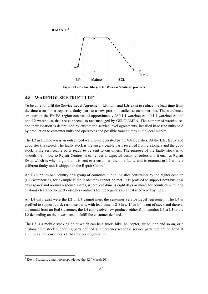
37

Figure 23 - Product lifecycle for Wireless Solutions' products

4.8 WAREHOUSE STRUCTURE To be able to fulfil the Service Level Agreement; L3s, L4s and L5s exist to reduce the lead-time from the time a customer reports a faulty part to a new part is installed at customer site. The warehouse structure in the EMEA region consists of approximately 250 L4 warehouses, 40 L3 warehouses and one L2 warehouse that are connected to and managed by GSLC EMEA. The number of warehouses and their location is determined by customer’s service level agreements, installed base (the units sold by production to customer units and operators) and possible transit times in the local market.

The L2 in Eindhoven is an outsourced warehouse operated by CEVA Logistics. At the L2s, faulty and good stock is stored. The faulty stock is the unserviceable parts received from customers and the good stock is the serviceable parts ready to be sent to customers. The purpose of the faulty stock is to smooth the inflow to Repair Centres, it can cover unexpected customer orders and it enables Repair Swap which is when a good unit is sent to a customer, then the faulty unit is returned to L2 while a different faulty unit is shipped to the Repair Centre5

An L3 supplies one country or a group of countries due to logistics constraints by the higher echelon (L2) warehouses, for example if the lead-times cannot be met. It is profiled to support next business days spares and normal response spares, where lead-time is eight days or more, for countries with long customs clearance to meet customer contracts for the logistics area that is covered by the L3.

An L4 only exist were the L2 or L3 cannot meet the customer Service Level Agreement. The L4 is profiled to support quick response parts, with lead-time is 2-8 hrs. If an L4 is out of stock and there is a demand from an End Customer, the L4 can receive new products either from another L4, a L3 or the L2 depending on the lowest cost to fulfil the customer demand.

The L5 is a mobile stocking point which can be a truck, bike, helicopter, air balloon and so on, or a customer site stock supporting parts defined as emergency response service parts that are on hand at all times at the customer’s field services organisation.

5 Kevin Kusters, e-mail correspondence the 12th March 2014

DEMAND

TIME

39

5 EMPIRICAL DATA The empirical data chapter gives the reader a basic understanding of the WHS Repair Logistics Flow. The chapter’s point of departure is a value stream map describing the process. After that, the governing structures, the warehouse structure and its planning and forecasting is described. The chapter ends with a total cost mapping of the WHS Repair Logistics Flow.

5.1 VALUE STREAM MAPPING For an overview of the WHS Repair Logistics Flow a value stream map has been created, seen in Figure 24. The actual ratio of value added time for a general service unit going through the flow is 0.037%. For calculations, see Appendix 1.

Figure 24 – Value Stream map of WHS Repair Logistics Flow

5.1.1 REQUEST FOR MATERIAL AUTHORIZATION (1) AND VALIDATION OF REQUEST FOR MATERIAL AUTHORIZATION (2)

The process starts with a customer placing a Request for Material Authorisation (RMA) electronically for the service part(s) needed. The customer in this case can be both an operator with its own field force making orders through a customer support contract, but it can also be a Wireless Solutions’ field force. Before this can be done however, a contract with a customer has to have been set-up in the WHS Delivery system. As contracts are left outside the scope, the contract implementation is left outside the value stream map as well. The receiver at Wireless Solutions examines the RMA and confirms that the products returned by the customer can be repaired at a Repair Centre within the organisation.

The next step is to check availability of the requested unit. After that, the RMA is verified and additional information is sent to the RMA issuer with information about a due date and address for shipment of the faulty unit.

40

5.1.2 CUSTOMER ORDER FULFILLMENT (3)

Depending on the lead-time requirement stated in the contracts, the orders are fulfilled either from an L5, L4, L3 or L2. The field engineers receive the good stock in a time span of two hours for the fastest service and 60 days for the slowest.

5.1.3 RETURN OF FAULTY PART TO L2 (4)

In most cases, the faulty parts are shipped directly to the L2. In some cases they are first consolidated at an L3 for further shipment to an L2, and sometimes when there is no L3 present, the parts can be directly shipped from an L4 to an L2. Lastly, there can be transports between L4 towards L3 and further on to the L2 as well. As the normal case is direct transport from customer to L2, that is has been used in the calculations of throughput time. The faulty parts are consolidated in the L2 where, on average, it is stored for about three months for parts repaired at Repair Centre Betamax. For NPI parts, the storage time in the faulty stock is shorter.

5.1.4 TRANSPORTATION L2 FROM REPAIR CENTRE (5)

When a RMA request from customers is received the good parts are shipped to the customer leading to decreasing inventory levels in good stock. The decrease triggers the creation of a RMA order towards Repair Centres to replenish the inventory levels either through new buy, reuse or repair. The parts are pushed to the Repair Centre where they are repaired. The main transportation mode is truck. The transport orders for shipments are created once a week towards Repair Centre Betamax and Repair Centre Kummle.

In some instances, the shipments are done directly from the L3 to the Repair Centres, however is this set-up not present in the EMEA region6 today.

5.1.5 TRANSPORTATION REPAIR CENTRE FROM L2 (6)

After repair, the parts are transported back to the L2. The transport frequency for both Repair Centres is three times per week. Parts from Repair Centre Betamax are stored in good stock on average 9 weeks and parts repaired at Repair Centre Kummle are stored in good stock on average 3 weeks7 until they are either pushed to replenish an L3 or pulled to fulfil a customer order.

5.1.6 FORECASTING (A)

Repair forecasts are performed centrally at the GSLCs by material planners and are communicated towards Repair Centres with a monthly frequency. The forecasting process is elaborated in 5.4.

5.2 PERFORMANCE MEASUREMENTS This section describes the governance structure in terms of the performance measurements used for the GSLC and the Repair Centres.

5.2.1 GSLC

There are several performance measurements for the GSLC EMEA organisation. The organisation is measured on Inventory Turnover, Capital Employed, Stock Availability, Customer Delivery 6 Viraj Joshi (Consultant, GSLC EMEA, Wireless Solutions AB), interviewed the 27th of March 2014 7 Kevin Kusters, e-mail correspondence the 10th of March 2014

41

Performance, Supplier Delivery Performance and End-To-End Turnaround Time (E2E TAT). The performance measurements, which are most important in this thesis are Inventory Turnover, Delivery Precision and E2E TAT.

Inventory Turnover

Inventory represents a big cost driver in the delivery of the service for the GLSC. Inventory Turnover measures how many times the whole inventory is re-used throughout a year. During the past years, the Inventory Turnover has become increasingly important for the WHS Repair Logistics Flow. Inventory Turnover is calculated based on the value of the inventory, which is called Average Spare Part Value. The formula is complex but is based on the price of buying the service unit new, the price of repairing it, and the total demand for that service unit. The Inventory Turnover figures are historically measured on the L2 echelon but as of 2014 it will be a performance indicator for the L3s and L4s as well. Inventory Turnover is the most important KPI for Material Managers.

Delivery Precision

As mentioned, the WHS Delivery is also measured on Delivery Precision and as seen in Figure 25 the organisation reached their goal in 2013.

YEAR GOAL RESULT GLOBAL

(WEIGHTED AVERAGE)

RESULT GSLC EMEA

2013 85% 96.6%

2014 95% 96,6%

Figure 25 - Delivery precision for WHS Operations 2013 and 2014

The remaining part of the ~5% is caused by a lack of good units on stock at the right warehouse. The main reasons for reduced delivery precisions are the behaviour by the end customer, prolonged lead-time by manufacturer on new buy orders, prolonged lead-time for Repair Centre on repair orders and poor planning at the GSLC.

End-To-End Turnaround Time (E2E TAT)

In addition WHS Delivery also measures the E2E TAT, which is the number of days from RMA creation at GSLC for repair of until the same part has been registered as back in L2 warehouse as a good part.

42

Figure 26 – The components of the E2E TAT

The E2E TAT is built up on the following components8:

• Picking/packing at L2 (1 day) • Request for Material Authorization to Repair Centre (1 day) • Shipping to RC (2 day for Europe) • Internal TAT at the Repair Centre (varies per Repair Centre and product group. Will be

described in 5.2.2) • Picking/packing at Repair Centre (1 day) • Shipment to L2 (varies between Repair Centres but approximately 2 days within Europe) • Receiving at L2 (1 day)

The E2E is therefore highly variable depending on factors such as product characteristics and distance between L2 and Repair Centre.

End-to-end Delivery Precision

The E2E Delivery Precision is significantly lower than the goals for Repair Centre Betamax and Kummle. During 2013, the result for Betamax was 81% and the result for Kummle was 65%, far below the target.

REPAIR CENTRE GOAL RESULT

Betamax 97% 81%

Kummle 95% 65%

Figure 27 – Delivery precision within the E2E TAT during 2013

5.2.2 REPAIR CENTRES

The Repair Centres are measured monthly on six KPIs by WHS Delivery. The KPIs are Turnaround Time, Delivery Precision, Quality, Volume Management, Backlog Management and Scrap. Below is a description of the most relevant KPIs in this thesis and how the calculations for each of them are made.

8Kevin Kusters, interviewed the 12th of March

43

Turn Around Time (TAT)

The purpose of TAT is to monitor the average lead-time in calendar days from receiving the units within the Repair Centre until the Repair Centre has requested pickup. The KPI is one of the most important KPIs for the Repair Centres. TAT is calculated according to the formula:

𝐿𝑒𝑎𝑑-𝑡𝑖𝑚𝑒 𝑓𝑜𝑟 𝑎𝑙𝑙 𝑢𝑛𝑖𝑡𝑠 𝑟𝑒𝑎𝑑𝑦 𝑓𝑜𝑟 𝑠ℎ𝑖𝑝𝑚𝑒𝑛𝑡 𝑑𝑢𝑟𝑖𝑛𝑔 𝑡ℎ𝑒 𝑚𝑒𝑎𝑠𝑢𝑟𝑒𝑚𝑒𝑛𝑡 𝑝𝑒𝑟𝑖𝑜𝑑 𝑑𝑎𝑦𝑠𝑇𝑜𝑡𝑎𝑙 𝑛𝑢𝑚𝑏𝑒𝑟 𝑜𝑓 𝑎𝑙𝑙 𝑢𝑛𝑖𝑡𝑠 𝑟𝑒𝑎𝑑𝑦 𝑓𝑜𝑟 𝑠ℎ𝑖𝑝𝑚𝑒𝑛𝑡 𝑑𝑢𝑟𝑖𝑛𝑔 𝑡ℎ𝑒 𝑚𝑒𝑎𝑠𝑢𝑟𝑒𝑚𝑒𝑛𝑡 𝑝𝑒𝑟𝑖𝑜𝑑 𝑢𝑛𝑖𝑡𝑠

(5.1)

Peaks in the TAT usually happen after summer and after Christmas holidays because a higher quantity of products are requested to be repaired before holidays to compensate for the lower output of the Repair Centres during these periods. It is the Repair Centres’ responsibility to communicate capacity fluctuations to the GSLCs if they think that their production baseline (the agreed monthly output of the Repair Centre) cannot be met (Internal document, 2013).

The target TAT for Repair Centre Betamax is 15 calendar days. The TAT has mostly been increasing throughout the last year, as can be seen in Figure 28 below, from well under the requirement of 15 calendar days in early 2013 to over 15 days both in October 2013 (15.04 days) and January 2014 (15.08 days). As can be seen there are sharp increases in TAT both in August and January, but since it is mostly handled within the agreed TAT, it is not considered a major problem.

Figure 28 - TAT at Repair Centre Betamax

The target TAT for Repair Centre Kummle is 10 calendar days, and as presented in Figure 29, the target TAT is only reached in four out of 11 months.

0

4

8

12

16

Days

44

Figure 29 - TAT at Repair Centre Kummle

Delivery Precision

The delivery precision shows the percentages of parts that were repaired within the contractual agreed TAT. In exceptional cases, the delivery precision can be based on OOLT, but these exceptions need to be approved between Vendor Delivery Management and the Repair Centre. The delivery precision is calculated according to the formula:

𝑁 − 𝑛𝑁

×100 [%] (5.2)

Where N is the number of units ready for shipment during the measurement period and n is the number of units ready for shipment that have a TAT longer than contractually agreed.

The delivery precision goal for Repair Centre Betamax is 97%. The Delivery Precision has been decreasing throughout the year. Only in February and March 2013 did the Repair Centre deliver on par with the set goals, see Figure 30 where the grey line is 97.5%. For the year 2013, the delivery precision was only 83.1% much due to delay of changes in products repair at the Repair Centre.

Figure 30 - Delivery Precision for Repair Centre Betamax

The delivery precision goal for Repair Centre Kummle is 95%, see the grey line in Figure 31. The delivery precision has steadily been increasing throughout 2013, as can be seen in Figure 31.

0

4

8

12

16

20

Days

0%

20%

40%

60%

80%

100%

45

Figure 31 - Delivery Precision for Repair Centre Kummle

Volume Management

This measurement shows the agreed baseline and the volumes that are received at the Repair Centre and the volumes ready for shipment in the measurement period.

The baseline is the expected or promised Repair Centre capacity. The inflow is the number of parts that a Repair Centre receives during a measurement period and volume ready for shipment is the number of parts that a Repair Centre has ready for shipment during a measurement period. The parts are ready for shipment when the Repair Centre has made a request for pickup.

The baseline forecast is a 12 month repair forecast where the average repair demand during the year is spread out over every individual month. The technical repair capacity is the maximum capacity of a Repair Centre on certain parts and/or product-groups based on available test-system/equipment (excl. resources). The test equipment’s utilization rate is set to 65% of the total shift time, excluding breaks and meetings. Repair Centre Betamax usually distinguishes between technical repair capacity and actual repair capacity, where the actual repair capacity is the capacity which they report to GSLC EMEA. Actual repair capacity is the lowest of the former and another where you take into account the capacity of personnel. As seen in Figure 32, the technical repair capacity is well above the baseline forecast, and only in October 2013 did the actually inflow tangent the technical repair capacity.

0%

20%

40%

60%

80%

100%

46

Figure 32 – Volume performance for Repair Centre Betamax

For Repair Centre Kummle the volume performance is presented in Figure 33. As can be seen is the technical capacity the bottle neck for Repair Centre Kummle only in June was the volumes ready for shipment lower than the technical repair capacity. This can handle by working overtime.

Figure 33 - Volume performance for Repair Centre Kummle

Backlog Management

The KPI gives an overview of the backlog situation at the Repair Centre. It also shows if the backlog is due to performance issues at the Repair Centre or due to areas related to Wireless Solutions (on hold). The measure shows how many parts that are on the premises of the Repair Centre and are exceeding the agreed TAT, as a snapshot. The parts are split into the categories backlog shorter than 30 calendar days, longer than 30 calendar days and units on hold. They are reported by the Repair Centre and approved by the Vendor Delivery Manager.

Baseline Forecast Actual In8low

Volume ready for shipment Technical Repair Capacity

Baseline In8low

Volume ready for shipment Technical repair capacity

47

For Repair Centre Betamax, the backlog is seen in Figure 34.

Figure 34 - Backlog Performance at Repair Centre Betamax

For Repair Centre Kummle, the backlog is seen in Figure 35 below.

Figure 35 – Backlog Performance at Repair Centre Kummle

5.3 INVENTORY PLANNING The material planners’ tasks are to plan the required orders for WHS Delivery. It is done by collecting data, doing a customer demand forecast which is used to decide required stock levels, and then plan how the orders should be sourced; either through new buy, reuse or repair. In order to understand the forecasting and the complexities it entails, an overview description of the planning is given.

5.3.1 CUSTOMERS’ BEHAVIOUR

As mentioned, customers’ actions influence the forecasts through their behaviour by how timely the faulty parts are returned to the L2. The customer usually has 14 calendar days from RMA approval to delivery of the faulty unit to the storage location (L2, L3 or L4). There are many late returns and an average return time of 14.2 calendar days for parts bound for Repair Centre Kummle (33% are returned too late) and 13.3 days on average for customers returning faulty parts repaired at Repair Centre Betamax (Internal document, 2014). Failure to deliver in time directly impacts the dimensioning by having a lack of faulty stock can lead to more new buy than necessary to make up for

Backlog Backlog > 30 days On-‐hold

Backlog Backlog > 30 days On-‐hold

48

the lack of faulty units. The result is excess stock once the faulty units are returned to the L4, L3 or L2. If new buy, which is more expensive then repairing, cannot fulfil the unexpected orders, the delivery precision can fall as a result which leads to penalties from customers towards Wireless Solutions.

Customers often order more units than needed because they don’t know how many faulty units they need to switch in their networks. The ordered products which are sent back to a warehouse are called the good return flow for which there is a forecast as well. Customers also do what is called batching which means that they store faulty products at their sites and just when they need to, they request many of the same parts, in many cases depleting the stock on hand (Internal Document, 2013). Since many L3 and L4 warehouses only keep stock of one of the same part number, this presents an issue.

To decrease the TAT for customer return, order management can implement a reminder mechanism. Moreover, there are contractual options for invoicing the customer for faulty service units that are passed the agreed return timeframe. The issue of batching is handled on a case by case basis and there is no record kept of how frequent the behaviour is9.

5.3.2 PLANNING FOR L3 AND L4

When a new part is sold to a customer, the contracted installed base is used as an input for a forecast since there is no historic data available. After three months, the software program in which planning and forecasting is performed considers there to be enough historic data to create a forecast based on historical data10. This switch is done partly because there is enough data, but also because the pricing mechanism in the service contracts does not consider installed base volumes but only the number of parts sent for repair. The consequence is that there is no incentive for customers to update the installed base values when they implement or de-implement parts in their networks.

Dimensioning of the L3s and L4s is done through a planning method called Multi-item Optimization which means that the target stock levels are calculated based on the installed base, service level targets by stock location for all parts that are positioned at that location, and uses cost and demand rate to evaluate the desired stock levels. The goal is to reach a 95% delivery performance on a system level, i.e. all parts combined, meaning that some parts can have a service level of 99% and others can have a service level of 60%.

The Target Stock Level is updated continuously with a specific frequency, but also when new contracts are implemented. During the updates, the Target Stock Levels are mainly based on: changes in demand, unit costs, mean time between failure (MTBF) and Inventory Turnover requirements. The installed base is however not updated continuously. Data of installed base for planning purposes are solely done as Customer Contract Implementation projects, which are performed for planning the L2.

5.3.3 PLANNING FOR L2

The L2 planning defines the stock levels at the L2 warehouses. The inputs are customer demand history, demand rates from L3s and L4s, faulty returns history, actual stock levels, order statuses, repair and new buy lead-times and the lifecycle of the product. The dimensioned stock levels on the parts kept at the L2 has a delivery performance of 95% on each individual part, i.e. not on a system

9 Kevin Kusters, e-mail correspondence the 31th of March, 2014 10 Kevin Kusters, e-mail correspondence the 11th of March, 2014

49

level as for the L3s and L4s. This is done as a safety procedure. If the Multi Item Optimisation tool would be used in L2 locations, it could lead to situations where an item is not stocked in any warehouse within the region and the lead-time to the customer would be longer than acceptable11.

When there is a new Customer Contract Implementation, there will be a purchase order for a quantity that secures delivery to customer for two months demand after the implementation. From then onward, the forecasting is done on historical demand. For small implementations with a large customer demand, new customers are added without making adaptations in the dimensioning of the inventories. The output from this planning process is a policy of safety stock and order recommendations. The order recommendations are for different types of orders: replenishment (allocation or transhipment) between warehouses, repair of faulty stock and whether to buy new stock or re-use material.

5.3.4 PLANNING THROUGH THE PRODUCT LIFECYCLE

Planning is related to the lifecycle of the product. The most difficult group to secure an even inflow for Repair Centres is the NPI product lifecycle as the volume of them will only increase with time, which leads to the faulty returns to the GSLC is immediately sent for repair as soon as possible. For mature and end of life products parts, there is a buffer on faulty stock which could act as a buffer to create a more even flow12.

5.4 FORECASTING AT GSLC EMEA The forecasting horizon is twelve months and the forecast period and frequency is one month. The forecasts are made on part level while the repair forecasts are aggregated to a product group level. The underlying data to make the forecasts are historical data and manual adjustments. The forecast accuracy has, and still is, an issue in the repair flow13. The formula informally used by the Repair Centres when comparing baseline and due dates is an inverse Mean Percentage Error (MPE) which will be used here too:

𝑀𝑃𝐸 =(𝐴! − 𝐹!)

𝐹! (5.3)

Where is the actual due dates when GSLC schedules a given part back at the warehouse in the Netherlands and is the forecasted volumes. Figure 36 shows the forecast accuracy on product group level based on previous month’s forecast compared with the due dates during the month.

Figure 36 – Forecast accuracy during 2013 for Repair Centre Betamax comparing previous month’s forecast with

actual due dates

11 Kevin Kusters, e-mail correspondence the 26th of March, 2014 12 Paul Paanen (Vendor Delivery Manager, WHS Operations, Wireless Solutions AB), e-mail correspondence the 19th of March 13 Jonas Henriksson (Manager Repair Centre, Repair Centre Betamax, Wireless Solutions AB). Interviewed 23th December 2013

Product group Jan Feb Mar Apr May June July Aug Sept Oct Nov Dec Average Average (abs) σBasic Line 5,18% -‐7,26% 32,81% 34,29% 8,14% 42,72% 42,06% 46,89% 56,92% -‐2,52% -‐2,03% 36,40% 24,47% 26,43% 0,22Inline -‐12,26% -‐13,67% -‐24,12% 81,75% 64,10% 13,33% 32,81% 19,57% 32,61% -‐22,97% -‐2,82% 3,77% 14,34% 26,98% 0,32URA1 -‐34,57% -‐10,98% -‐22,83% 33,33% -‐55,38% -‐40,82% -‐12,31% -‐47,83% -‐16,39% -‐52,50% -‐35,14% -‐34,09% -‐27,46% 33,01% 0,23URA2 -‐27,96% -‐24,66% -‐2,91% 2,01% -‐9,81% 11,10% 14,90% 22,74% 16,15% 0,88% -‐11,17% 17,77% 0,75% 13,51% 0,16Traffic Line -‐10,74% -‐17,59% 13,40% -‐29,01% -‐17,75% 15,38% 20,26% 15,01% 7,46% 59,27% -‐5,83% 16,49% 5,53% 19,02% 0,23TRL -‐45,45% -‐88,89% 24,00% -‐45,45% 42,86% 2,86% 83,33% 7,14% 200,00% 79,31% -‐13,89% 41,67% 23,96% 56,24% 0,72Montly sum -‐20,97% -‐27,17% 3,39% 12,82% 5,36% 7,43% 30,18% 10,59% 49,46% 10,24% -‐11,81% 13,67% 6,93% 29,20% 0,31

50

Black boxes indicate values where:

MPE < −20% | MPE > 20% (5.4)

Grey boxes indicate values where:

−20% < MPE < −10% | 10% < MPE < 20% (5.5)

And white boxes indicate values where:

−10% < MPE < 10% (5.6)

Internal Repair Centres are expected to handle deviations of 20% from the baseline during one consecutive month which explains the colour structure. Moreover, for Repair Centre Betamax, additional costs are generally incurred in the grey boxes with forecast errors between 10%-20%. The figure shows that the forecast error was less than 10% in 15 out of 72 occasions and between 10%-20% in 20 occasions out of 72 which in total is less than half of the total instances during 2013. Inline, URA2 and Traffic Line had the lowest total forecast error aggregated over the year. All product groups except URA2 had a forecast bias, albeit URA1, Basic Line and TRL are clearly more biased than the others. In total, there is a forecast bias (under-forecasting) of approx. 7% throughout the year.

The capability for Repair Centre Betamax and Kummle in reacting to changes in demand is dependent upon the lead-time to acquire resources in forms of trouble-shooters, repair personnel and test equipment which is approx. 3 months or longer. A more meaningful comparison is therefore the forecast three months ago and the actual due dates, presented in Figure 37.

Figure 37 - Forecast accuracy during 2013 for Repair Centre Betamax comparing forecast made three months earlier

with actual due dates

The figure shows that the forecast error was less than 10% in 11 out of 72 occasions and between 10%-20% in 13 occasions out of 72 which in total is one third of the total instances during 2013. Basic Line and URA2 had the lowest total forecast error aggregated over the year. All product groups had a forecast bias and in total, there is a forecast bias (over-forecasting) of approx. 5% throughout the year. The total MPE went from 29% to 45% from Figure 36 to Figure 37.

For Repair Centre Kummle the nature of the NPI products makes the demand volatile, which increases forecasting difficulty. This is shown in Figure 38.

Product group Jan Feb Mar Apr May June July Aug Sept Oct Nov Dec Average Average (abs) σBasic Line -‐36,76% -‐14,33% 15,18% 19,15% -‐22,20% -‐1,94% -‐18,93% -‐11,78% 21,04% -‐8,31% 13,04% 3,79% -‐3,50% 15,54% 0,18Inline -‐30,61% -‐52,19% -‐45,80% 55,63% -‐45,30% 0,00% -‐24,11% -‐66,26% -‐56,74% -‐32,94% -‐25,00% -‐42,71% -‐30,50% 39,77% 0,31URA1 -‐53,91% -‐32,41% -‐47,79% 3,60% -‐75,00% -‐68,82% -‐6,56% -‐29,41% 15,91% -‐64,15% -‐50,00% -‐38,30% -‐37,24% 40,49% 0,28URA2 -‐40,82% -‐45,56% -‐27,27% 0,85% -‐58,24% -‐34,77% 22,31% 23,46% 50,69% 5,46% -‐9,67% -‐26,13% -‐11,64% 28,77% 0,31Traffic Line -‐32,76% -‐51,32% -‐12,36% -‐26,09% -‐65,77% -‐10,05% 3,58% 14,69% -‐12,99% -‐17,50% -‐11,95% -‐50,00% -‐22,71% 25,76% 0,23TRL -‐72,73% -‐96,00% 82,35% 421,43% 5,26% 33,33% 94,12% 136,84% 305,88% 116,67% -‐45,61% -‐39,29% 78,52% 120,79% 1,48Montly sum -‐44,60% -‐48,64% -‐5,95% 79,09% -‐43,54% -‐13,71% 11,74% 11,26% 53,97% -‐0,13% -‐21,53% -‐32,11% -‐4,51% 45,19% 0,46

51

Figure 38 - Forecast accuracy during 2013 for Repair Centre Kummle comparing forecast made three months earlier

with actual due dates

The figure clearly shows that the MPE has almost tripled (84%) compared to the same time frame for Betamax. For XRU and UTC, the actual due dates can increase quickly as seen in the encircled areas. Furthermore, there were forecast figures for a product group named “Not Defined” which never appeared among the due dates.

5.4.1 PROCEDURE

All customer demand figures from up to 36 months are summed to create a demand forecast for the next coming twelve months. The demand forecast represents the total demanded volume from customers. As mentioned, demand can be fulfilled through repair, new buy and reuse which results in creation of forecasts for these as well. There are two repair forecasts; an operational and one baseline forecast. The operational forecast is the monthly forecast with the due dates during each month. The baseline forecast is a 12 month forecast where repair demand is flattened. Other forecasts created are the good return forecast, new-buy forecast and reuse forecast. Even if the thesis has scoped it only towards the repair forecasts, the complexities of creating an accurate repair forecast are affected by the rest of the system.

The forecasts are performed on every “prime” part, which is the highest successor within a given part chain represented by the underlined part IDs in Figure 21, page 43. The forecasts for the prime part is the consolidated demand for the prime part and the predecessors in any given part chain, e.g. for Part chain I in Figure 22 on page 44, the forecast for part ID III is for the combined demand of part ID I, part ID II and part ID III. Parts within every part chain are seen as replacements of each other, e.g. if a customer returns a newer version of a product still within the same part chain it can receive a lower version within the same part chain and vice versa.

Forecasts toward Repair Centres can be divided into four different aggregation levels, presented in Figure 39. Every region is first defining the forecast on part number level. In the second step, the parts are distributed into the product groups. The third aggregation level is the forecast for the whole region, in this scope EMEA. The Vendor Delivery Manager aggregates all forecasts into a tool called FAME to create the total consolidated forecast which is sent to Repair Centres.

Product group Apr May June July Aug Sept Oct Nov Dec Average Average (abs) σXDU -‐41,36% -‐27,02% -‐52,12% -‐38,46% 14,57% -‐16,76% -‐1,41% -‐4,68% 6,72% -‐17,84% 22,57% 0,22XRRU -‐91,51% -‐69,06% -‐76,54% -‐43,71% -‐78,07% -‐81,25% -‐67,55% -‐61,80% -‐85,54% -‐72,78% 72,78% 0,13XRU 20,09% -‐42,73% -‐69,44% -‐16,39% -‐3,73% -‐25,47% 368,09% 365,31% 209,62% 89,48% 124,54% 1,66UTC 100,00% 100,00% -‐71,43% -‐87,50% 33,33% 220,00% -‐100,00% -‐100,00% -‐90,91% 0,39% 100,35% 1,11RAI -‐100,00% -‐100,00% 100,00% 0,00Montly sum -‐3,20% -‐9,70% -‐67,38% -‐46,52% -‐8,47% 24,13% 49,78% 49,71% -‐12,02% -‐2,63% 84,05% 0,37

52

Figure 39 – Forecast aggregation levels (based on van Dueren den Hollander)

FAME

FAME is a software that allows GSLC material planners to make small manual adjustments and add comments to the forecasts that is extracted of the planning tool before sending it to the Vendor Delivery Manager. Furthermore, it allows the Vendor Delivery Manager to aggregate all GSLC’s forecasts into one forecast per vendor in the same format and communicate with the vendors clearly. Also, it is dynamic in the way that it allows users to elaborate with the forecast per part, product group, GSLC and Repair Centre. There is also a proposal for implementing a forecast accuracy calculation in the software14.

5.4.2 BASELINE

The baseline is the expected or promised Repair Centre capacity. It is based on historical demand, the 12 month baseline forecast and strategic decisions. Strategic decisions can be factors like stage in product lifecycle, if the repair is going to be moved from a Repair Centre to another and so on. For external Repair Centres, the baseline is set with a horizon of one year and is updated yearly. For Repair Centre Betamax and Repair Centre Kummle, the baseline is updated every month. For external Repair Centres, the actuals are allowed to deviate:

𝐴! = 𝐵𝑎𝑠𝑒𝑙𝑖𝑛𝑒! ± 0.3×𝐵𝑎𝑠𝑒𝑙𝑖𝑛𝑒! (5.7)

For a consecutive of maximum one month. For internal Repair Centres, the actuals are allowed to deviate:

𝐴! = 𝐵𝑎𝑠𝑒𝑙𝑖𝑛𝑒! ± 0.2×𝐵𝑎𝑠𝑒𝑙𝑖𝑛𝑒! (5.8)

For a consecutive of maximum one month. For Repair Centre Betamax, the baseline figure is divided by 4.3. The output is a baseline for each week during the month.

The baseline should be set during the Monthly Business Review meeting where the Vendor Delivery Manager, the planner at the Repair Centre, his or her manager and also a representative from Repair

14 Kevin Kusters, e-mail correspondence the 10th of March, 2014

53

Solutions decide on a baseline for the following month. In the end it is the Vendor Delivery Manager that has the last saying in deciding the baseline. Through interviews with actors in the flow, the authors have discovered that the routines associated with the baseline process are not always done properly with double work related to forecasting as a result.

5.4.3 SOFTWARE

The software that is used for material planning purposes is called Xelus. The software calculates the right mix of parts in the right location to meet demand for scheduled and unscheduled maintenance. Xelus also has a forecasting module connected to it in addition to the main planning module. The software aims to reach the Target Stock Levels and achieve a 95% system service level on the L3s and L4s and a 95% individual part service level on the L2. Based on this, the software gives recommendations to the planners every day for what it thinks is an appropriate action based on the chosen forecast.

Issues with the software

There are several identified issues with the planning software Xelus, identified by planners15;16:

• Xelus sums up the need for a whole month, and recommends actions to receive a good part to the L2 (the due date) warehouse on the 1st of a given month. This results in a batch of orders that are proposed to the planner long before they are actually forecasted to be needed in the warehouses

• According to a planner, the Target Stock Level are often set too high and manual intervention is needed in order to increase the Inventory Turnover and still keeping the 95% service level goal

• The software can only use historic demands to conjure a forecast. The missing leads to manual adjustments

• Xelus have the potential to take supplier downtime like holidays into consideration, but it does not understand that there should be an increased output from the Repair Centre before the holiday to cover up the downtime during the holidays

5.4.4 FORECASTING METHODS

The forecasting at WHS Delivery is almost solely based on time series forecasting, except for the first three months of a new product implementation. In Xelus, the planner has approximately 30 methods to choose from when calculating the forecast. Examples of methods to choose from are different variants of moving average, exponential smoothing and Croston’s method among others. However, the software automatically recommends a method based on previous demand periods which the planner can decide to use if he or she wants.

Depending on the situation, the planners can use four different variables which change the way the calculations are done. Firstly, the historical period determines how many periods of historic data to take into account. Secondly, weighting to determine how much last period’s demand is taken into account compared to the previous periods. Thirdly, volume can be used as a parameter to determine

15 Kevin Kusters, interviewed the 29th of April, 2014 16 Mustafa Senturk, interviewed the 28th of April, 2014

54

forecast methods. Lastly, if there are trends or seasonal patterns, there are specific methods to take this into account like double smoothing and triple exponential smoothing.

Manual adjustments can be done in several stages of the process. Either, the planner sees that a forecast does not align with the trajectory based on the historical data. Without other external input that can be a sign of suspicion. Also, there can also be notes in Xelus by personnel working in delivery management when there are significant installed base changes which can be used to manually fit the right forecast with the projected increase in installed base. If the Vendor Delivery Manager sees something suspicious after receiving the forecast he can discuss the issue with the planner. In the end however, it is the planner who is responsible for the forecast while the Vendor Delivery Manager is held accountable17.

5.4.5 CROSS-FUNCTIONAL INTEGRATION

There are several functions and organisations directly or indirectly involved in the forecasting process and its results. The function which is responsible for implementing new contracts which will be supported from the L3s and L4s has access to new installed base figures and they can be communicated as a text note to planners. This only happens when there is an exemption in the volumes of the installed base of which the planner can choose to take into account if he wants to.18

There is no direct connection between Finance, Customer Management, Material Management and Vendor Delivery Management with regards to forecasting. There are no structural meetings planned on forecasting. Even though the functions of Vendor Delivery Management and Material Management do not collaborate, there is operational coordination regarding the forecasting between the Vendor Delivery Manager and the planner related to the same Repair Centre, but it is still on resource-to-resource level and not functional.

There are own forecasting efforts by different actors. The material planner is the official creator of the forecast; the Vendor Delivery Manager receives it but can propose and make changes. Moreover, when deciding upon the baseline there is additional data that is taken into consideration before deciding on what capacity should be promised throughout the month or year. When the baseline is decided, the planner is never present. There is no accountability within any function for forecasting. There is only indirect accountability for the Material Planner and Vendor Delivery Manager due to the mechanism of the baseline where one of the inputs is the forecast, and if the difference is too large, the issue can be escalated.

5.4.6 APPROACH TO FORECASTING

There is no structural categorisation done on the parts in terms of having a clear-cut differentiation of methods except for the four different variables described in 5.4.4. The choices of forecasting methods are quite static independent on the maturity phase, volume and general demand characteristics. There is a general knowledge of the most common forecasting methods, but no overall understanding of the methods. Forecasting is viewed as a tactical function, and it is more “something that needs to be done” (Van Dueren den Hollander, 2014) rather than understanding of the importance of forecasting for the Repair Centres, logistics service providers and other stakeholders’ to be able to plan. Forecasting can be considered to be quite a automated activity. 17 Kevin Kusters, e-mail correspondence the 23th of April, 2014 18 Kevin Kusters, interviewed the 29th of April, 2014

55

5.4.7 FORECASTING IT-SYSTEMS

There is forecasting software included in the planning system Xelus. The information from Xelus where the forecast is made is transferred smoothly to FAME from where it is sent to Repair Centres. Vendor Delivery Management personnel can do their own forecast accuracy analysis. There is no consensus on how to measure forecast accuracy so there is partly an island of analysis situation, albeit not in the forecasting procedure itself.

5.4.8 PERFORMANCE MEASUREMENTS

Forecast accuracy and forecast deviation is not measured. Forecast deviation is difference between a forecast from month to month. As mentioned however, the delta between the baseline and the actuals are somewhat semi-structurally measured by Repair Centre Betamax. The measurement is not based on the actuals but instead on the inbound delivered to the Repair Centre during a specific month. Looking at the same time period as in chapter 5.4 when measuring forecast accuracy, Figure 40 and Figure 41 is the result of the Repair Centre Betamax’ measurement:

Figure 40 - Forecast accuracy based on forecast three months in future and inbound deliveries

In Figure 40, the total forecast accuracy is similar to Figure 37 as is expected, but on a monthly level differences occur. The differences are small when comparing forecast accuracy between Figure 36 and Figure 41 in terms of number of months with acceptable forecasts (within +-20%), but the percentage values change from month to month.

Figure 41 - Forecast accuracy based on forecast one month in future and inbound deliveries

Figure 37 indicates a large total difference in the way of measuring. Furthermore, Repair Centres plan in buckets of weeks and the forecast accuracy on this level is displayed in Figure 42 below. The standard deviation (σ) has almost doubled compared to the inbound deliveries on a monthly basis, all other factors equal.

Product group Jan Feb Mar Apr May June July Aug Sept Oct Nov Dec Average Average (abs) σBasic Line -‐20,56% 5,79% 1,90% 5,92% -‐19,76% -‐10,97% -‐11,20% 14,94% -‐5,49% -‐1,78% 29,10% 37,61% 2,13% 13,75% 0,17Inline -‐32,14% -‐58,57% -‐55,04% 43,13% -‐10,26% -‐42,94% -‐32,14% -‐58,28% -‐75,18% -‐20,00% -‐23,91% -‐35,42% -‐33,40% 40,58% 0,29URA1 -‐38,26% -‐34,26% -‐75,00% 8,11% -‐87,93% -‐41,94% -‐16,39% -‐21,57% -‐25,00% -‐56,60% -‐33,33% -‐61,70% -‐40,32% 41,67% 0,25URA2 -‐38,09% -‐36,69% -‐36,19% -‐15,46% -‐51,70% -‐23,02% 33,82% 35,85% 29,53% -‐5,92% -‐19,52% -‐33,97% -‐13,45% 29,98% 0,29Traffic Line -‐54,53% -‐16,50% -‐30,60% -‐49,09% -‐31,53% -‐26,81% 15,44% -‐22,60% 39,88% -‐29,67% -‐41,30% -‐29,91% -‐23,10% 32,32% 0,25TRL -‐95,45% -‐8,00% 264,71% 114,29% 94,74% -‐11,11% 258,82% 231,58% 158,82% 83,33% -‐77,19% -‐28,57% 82,16% 118,88% 1,22Montly sum -‐46,51% -‐24,70% 11,63% 17,82% -‐17,74% -‐26,13% 41,39% 29,99% 20,43% -‐5,11% -‐27,69% -‐25,33% -‐4,33% 46,20% 0,42

Product group Jan Feb Mar Apr May June July Aug Sept Oct Nov Dec Sum Average (abs) σBasic Line 32,12% 14,52% 17,50% 19,37% 11,53% 29,58% 55,61% 91,39% 22,53% 4,42% 11,88% 80,84% 32,61% 32,61% 0,27Inline -‐14,19% -‐25,18% -‐37,06% 81,75% 169,23% -‐35,33% 18,75% 47,83% -‐23,91% -‐8,11% -‐1,41% 16,98% 15,78% 39,98% 0,57URA1 -‐12,35% -‐13,41% -‐63,04% 33,33% -‐78,46% 10,20% -‐21,54% -‐42,03% -‐45,90% -‐42,50% -‐13,51% -‐59,09% -‐29,03% 36,28% 0,31URA2 -‐24,64% -‐12,39% -‐14,81% 2,01% 4,31% 31,12% 25,71% 35,05% -‐0,16% -‐10,00% -‐20,86% 5,27% 1,72% 15,53% 0,19Traffic Line -‐39,64% 41,38% -‐10,20% -‐29,01% 64,51% -‐6,11% 34,03% -‐22,38% 72,76% 35,76% -‐37,22% 63,30% 13,93% 38,02% 0,41TRL -‐90,91% 155,56% 148,00% -‐45,45% 164,29% -‐31,43% 238,89% 50,00% 91,30% 51,72% -‐63,89% 66,67% 61,23% 99,84% 0,99Montly sum -‐24,93% 26,75% 6,73% 10,33% 55,90% -‐0,33% 58,57% 26,64% 19,44% 5,22% -‐20,83% 28,99% 16,04% 43,71% 0,46

56

Figure 42 - Summary of the forecast accuracy for 2013 using weekly planning buckets for three months into the future

5.5 CONSEQUENCES OF FORECAST DEVIATION When volumes are more than 20% over baseline, it is normally managed by overtime, but occasionally not even overtime helps to handle the extra volumes due to capacity constraints. This in turns generates lack in reaching the target delivery precision and in the end can affect the serviceability of the whole value chain. When the volumes are lower than baseline, the unused capacity is not downsized flexibly, so it is just a waste.

5.5.1 COPING WITH THE DEVIATION

To cope with the variation of inbound flow of material between +20% and -20% of the baseline there is flexibility within the system. In times of increased volumes than expected overtime and increased production pace can be implemented. However, complications arise when the volumes reach above and below these limits and to some extent even at a variation of +-10%19.

Both Repair Centre Betamax and Kummle are located in the same facility as new production which generates possibilities to move blue collars between the different production units whenever there is an actual demand higher or lower than the planned volumes. Furthermore. Repair Centre Kummle can put resources onto repairing Claims. Claims are parts where finding the fault and learn to repair the product is crucial. They are not as time-sensitive but the Repair Centre can operate on them when there is time, minimizing the risk of running low on repair work at the Repair Centre. This hedging is however an uncertain process. Firstly, additional work force needs to be required somewhere and secondly, the employee needs to have the right knowledge to handle the work on another production unit. Other measures that used to be an option are to terminate consultants. However, today there are no longer consultants used in the repair production. All these measures must also be administrated which just as unused capacity can be seen as an unnecessary cost.

5.5.2 LEVELLING TODAY

None of the Repair Centres implemented the OOLT concept described in 3.7.2 due lack of profitability. What Repair Centres Betamax however has done is to build up a buffer of approximately one week of parts that can be used to level the production. This is possible because time from a unit is picked for repair until ready for shipment is only approximately 8 calendar days and the internal TAT is 15 days.

19 Jonas Henriksson B, interviewed the 7th of May, 2014

Planning object Average Average (abs) σBasic Line -‐4,04% 32,65% 0,40Inline -‐32,16% 54,21% 0,50URA1 -‐37,72% 56,11% 0,57URA2 -‐12,78% 39,60% 0,49Traffic Line -‐23,22% 47,25% 0,53TRL 74,17% 145,72% 2,59Montly ABS sum 38,82% 38,82% 0,85

57

5.5.3 PREREQUISISTS FOR INTRODUCING OOLT

The current situation state that OOLT is not supported unless a separate assignment is written and signed by the Repair Centre, GSLC and Repair Solutions. Furthermore, any decision to implement OOLT shall be supported by a firm business case. Handling OOLT comes with a change of working and ways of measuring the most important KPI for the Repair Centre namely TAT. Due to the fact that orders are created with a due date longer that the E2E TAT, measurement of the TAT would not be feasible since it would not reflect the actual performance. While exploring the outcome of the previous investigations further it has been showed that current state of working differs from when investigations were done.

5.6 TOTAL COST ANALYSIS Since the scope of this paper considers only internal Repair Centres the cost and revenue structure is considered somewhat different than looking at an external supplier of repair services. The Repair Centres today are acting in terms of cost forwarding. This means that the cost they carry should be covered by what they charge for conducting the repair i.e. they should theoretically not make a profit. The costs are grouped into two main cost components, direct and indirect cost. These costs then forms a total cost which is used to set the price for repairing a certain unit. Direct and indirect cost adds-up of several different sub components such as packaging material, component cost, man hour for repair and test, rent of machinery, administrative work, material handling etc.

For the ability to make an assessment of the supply chain from a total cost concept point of view the cost carried today by the different actors in the supply chain needs to be broken down and merged in terms of cost items related to the total cost concept.

5.6.1 CUSTOMER SERVICE DIMENSION

The scope of investigation concerns an aftermarket supply chain where the service level is considered important. However, due to the delimitations of the scope, cost for not fulfilling the contracts is unknown and has not been taken into consideration.

5.6.2 INVENTORY CARRYING COST

The inventory carrying cost for the WHS Repair Logistics Flow has been mapped and calculated in terms of capital cost, inventory service cost, storage cost and inventory risk cost, see Figure 43, all to be described further on.

Capital cost

The capital cost of inventory is calculated by using a global average Inventory Turnover related to the total amount of units handled in inventory for each Repair Centre respectively. The average Average Spare Part Value has then been multiplied by the volume to provide a total yearly value which is multiplied with an assumed internal rate of 15%.

Inventory service cost

The inventory service cost is calculated from cost of handling material for inbound and outbound deliveries. There are four types of flows that generate cost in terms of repack, unit handling etc., which varies depending on the amount of units handled. These flows are the inbound of faulty parts from the

58

End Customer, outbound of faulty part to the Repair Centres, inbound of good units from the Repair Centres and outbound of good units to the end customer.

The cost data regarding these actions are built upon a total annual cost related to the total amount of parts handled in each flow. By dividing the total cost for a specific flow with the total amount of parts handled in that flow it is possible to generate a cost per part that can be related to the volume handled for Repair Centre Betamax and Kummle.

Within the inventory service cost there is also cost items related to discrepancy handling, packaging material, stock control and a fixed fee related to IT solutions. These costs have also been related to the volume of units handled for Repair Centre Betamax and Kummle.

Storage space cost

At GSLC EMEA the storage space cost is built upon a total cost for warehouse space, depending on the number of unit handled. This gives a warehouse cost per part that can be related to the volume managed for Repair Centre Betamax and Kummle. In addition to the storage space cost for GSLC EMEA, Repair Centre Betamax keep a buffer of 0-7 calendar days and Repair Centre Kummle level the production with repair of Claims.

Inventory risk cost

Inventory risk cost relates to the risk of having inventory in terms of obsolesce, theft, relocation within the inventory and damage of inventory (Lambert et al., 2005). Within the scope of this thesis inventory risk cost has been left out from a quantitative perspective. Obsolescence is however a concern for the good stock inventory which is elaborated further in chapter 6.

59

Figure 43 - Definition of inventory carrying cost

5.6.3 WAREHOUSE COST

All costs related to warehousing has been placed under inventory carrying and storage space costs because there is no clear distinction between how the warehouse cost and inventory cost are presented in the analysed data.

5.6.4 LOT QUANTITY COST

In the cost model presented in the theory chapter the decision has been taken to remove the purchasing cost from the lot quantity cost. This is mainly due to the fact that purchasing is centralised for the whole factory and not only for the repair process. In the lot quantity cost item the two main cost components calculated are the material cost in terms of components used in the repair production and packaging material for the two Repair Centres, see Figure 44.

Since Repair Centre Betamax and Repair Centre Kummle is handling parts from all the current GSLCs the total lot quantity cost presented in their profit and loss account can be related to all products. To get a somewhat representative cost related to GSLC EMEA the percentage of units handled for GSLC EMEA has been used to define the cost.

60

Figure 44 – Definition of lot quantity cost

5.6.5 ORDER PROCESSING AND INFORMATION

To generate an understanding of the order processing and information costs the indirect costs at the Repair Centres have been used. These costs are based on the cost for administration but also consider the cost for personnel managing the registration and unpacking of incoming goods as well as picking and packing outgoing goods, see Figure 45. The total cost is grouped and divided among the total amount of units handled at the Repair Centre to get a unified profit base overhead that is added upon the repair price of each unit.

In addition to the order processing and information cost at the Repair Centres there is also a need to include the overhead costs at GSLC EMEA. These figures have not been given and an assumption has been made to establish cost for handling order processing and information activities.

Figure 45 - Definition of order processing and information cost

5.6.6 TRANSPORTATION COST

Almost all cost for transportation is carried by GSLC EMEA centrally. This includes all transportations to and from the different Repair Centres but also to some extent transportations to and from the End Customers, as seen in Figure 46. In the inbound flow of faulty parts from the customers, GSLC EMEA holds approximately 28% of the cost while the rest is paid by the customers. The outbound cost is not covered within the scope of investigation and is thereby not taken into consideration.

The GSLC outsources the transportation to a Logistics Service Provider where the cost is contracted in terms of chargeable weight. The chargeable weight is determined by the highest weight when comparing volumetric weight with actual weight. The volumetric weight depends on a dimension factor which is used to convert the volume to volumetric weight. The industry standard is usually 6000 cm3/kg or 167 kg/m3, Wireless Solutions has contracted the use of 167 kg/m3 with its Logistics Service Provider20. For every shipment there is a start tariff for the first chargeable kilo and then a separate tariff for each additional kilo added. The cost of these tariffs is based on service level, i.e. speed of delivery and mode of transport. The mode of transport is mostly road and air where the Logistics Service Provider itself most often decides the mode of transport. 20 Viraj Joshi, interviewed the 27th of March 201

61

The total transportation cost is calculated with data including city of origin, city of destination, number of units per shipment and cost per shipment. In this case it was only possible to get the total amount of parts and cost i.e. not separated by origin or destination. For calculation purposes the total amount charged was set in relation to the percentage of units handled towards Repair Centre Betamax and Kummle, generating a cost for the inbound flow.

In addition to the actual transportation cost carried by the GSLC there are some minor administration fees carried by each Repair Centre. This is due to system and contract constrains, making the Repair Centres use one Logistics Service Provider for the booking of transportation and another one for the actual transport.

Figure 46 - Definition of transportation cost

5.6.7 PRODUCTION COST

The production cost is considered the cost that is directly related to the production. This cost includes blue collar salary and overhead, such as machinery and premises rent. Production cost is calculated out of the total cost for repair and test handled by Repair Centre Betamax and Kummle respectively in relation to EMEA volumes.

5.6.8 COST OVERVIEW

The breakdown of the costs related to both Repair Logistics Flows is presented in Figure 47 and Figure 48 below. The figures only show five cost categories since the cost for the customer service dimension was not taken into consideration and warehousing cost was moved to inventory cost.

The order processing and information cost related to Repair Centre Kummle calculated within the costs of production. Except from that, it can be seen that the spread of cost and the drivers are somewhat similar between the both Repair Centres. The main cost driver is related to production and order and information cost, followed by the lot quantity cost.

62

Figure 47 – Total Supply Chain Cost Repair Centre Betamax

Figure 48 – Total Supply Chain Cost Repair Centre Kummle

63

6 ANALYSIS The analysis chapter firstly gives the reader a general analysis of the current state. Improvement areas are identified related to planning and forecasting. Furthermore improvement strategies for handling the effects of the current situation are elaborated on.

6.1 CURRENT STATE ANALYSIS Srivastava (2012) describes the potential of the aftermarket supply chain in terms of high profitability. Looking at the WHS Repair Logistics Flow there are several attributes that can be related to how Cohen et al. (2006) describe the aftermarket. Even though many aspects align, the most important one can be related to the sporadic and uncertain demand. Within the WHS Repair Logistics Flow this demand uncertainty is a result of several different aspects. Firstly, there is an enormous wide range of products that is contracted for service. The service agreement also stretches over the entire product lifecycle. Secondly, the contracted lead-time to serve customers can vary between two hours up to 60 days.

To meet the requirements generated by the environment in which WHS Repair Logistics Flow exists, certain strategies and operating philosophies are in use. As acknowledged in the empirical chapter, the GSLC meets the uncertain demand and highly variable contracted lead-times by having high volumes of inventory in multiple locations close to the customer with flexible capacity. A sign of the high demands put on the WHS Repair Logistics Flow is the relatively low percentage of value added time of 0.037%. In relation to the KPIs measured on Material Management (Inventory Turnover, Capital Employed, Stock Availability, Customer Delivery Performance and Supplier Delivery Performance), it becomes evident that all parts in the total value matrix provided by Johansson et al. (1993), see formula (3.1) on page 15, are measured. The most important aspect however is the service level towards the customers which is proven by the fact that all entities in the WHS Repair Logistics Flow are measured on service level in terms of Delivery Precision. The conclusion drawn from this is that WHS Repair Logistics Flow is responsive.

Taking this aspect in relation to Mason-Jones et al. (2000) the market winner of the WHS Repair Logistics Flow is the service level offered to the customers. Cost, quality and lead-time are also considered important aspects but, in the context of Wireless Solutions, these aspects are merely standard capabilities required to enter the market. To understand the rationale behind this, it is important to understand the products provided by Wireless Solutions. The products are part of forming a network infrastructure which, make the network availability critical to the customers’ customer.

Looking at the E2E lead-time however, there is no usage of inventory to hedge against the variable demand and no time adjustment. The Repair Centres are forced to use capacity to handle the inbound variation, which is not enough as it can be seen that the Delivery Precision is 81% for Repair Centre Betamax during 2013 and 65% for Repair Centre Kummle, far below the targets of 97% and 95%. The high forecast deviation in the combination with lacking hedging mechanisms creates an even higher demand for excessive capacity to handle the variations in inbound deliveries to Repair Centres.

6.1.1 THE SYSTEM VIEW

The good and faulty stock kept at the L2 can be used in order to separate production pace from demand pace and thereby increase the possibility to smoothen repair production. The faulty stock

64

buffer is kept for the ability to send repair orders when a replenishment of the good stock is needed while the good stock buffer is there to serve the customers’ need rapidly. Within the current system, the L2 inventory works as a clear decoupling point between the customers and the Repair Centres. The customers in terms of warehouses and Customer Units are served directly from stock by the GSLC while the Repair Centres provide the GSLC with services based on orders. These orders are shipped from the GSLC to the Repair Centres in a MTO environment. The system setup however does not generate levelling possibilities, which Naylor et al. (1999) describe as a beneficial outcome of working with buffers at the decoupling point. Instead, the variation is transferred to the Repair Centres. The fluctuations in the End Customer demand is transferred to the demand of repair for the Repair Centre where the Repair Centre has an internal TAT that can be used for levelling. However, when the volumes deviate too much from forecast this time buffer does not provide the levelling function needed.

Isolating the issue of variable demand to the Repair Centre one can start elaborating on ways to reduce the variation and generate possibilities for the Repair Centre to become more cost-efficient. Today there are high costs associated to overcapacity in machinery and shop floor space, as well as non-value adding working hours and overtime for the employees. This can also be seen in the cost breakdown isolated to the Repair Centres. Machinery and premises stand in direct link to each other since taking machinery away means enabling utilisation of floor space for other purposes or subletting. Together these parameters contribute to approximately 40% of the total cost at Repair Centre Betamax, which also is the largest cost item for that supply chain.

6.1.2 REPAIR CENTRE’S SITUATION

According to Fisher (1997), when managing a responsive supply chain the suppliers should not be chosen for their low cost but for their speed and flexibility. The flexibility for the Repair Centres is contracted to ensure that they possess capacity to handle actual demand within the agreed deviation of +-20% for a maximum of one month. This is done to ensure serviceability also during peaks in demand of repair, as explained in chapter 5.5.1, in forecasting abilities aligned with volatile and unpredictable demand. This type of overcapacity creates costs which place the Repair Centres in a trade-off situation where having excess capacity and flexibility is needed but at the same time provides a high cost efficiency to stay competitive, because the Repair Centres, even internal ones, are sourced as a supplier by Repair Solutions.

An additional aspect mentioned earlier, is also the fact that the Repair Centres invoice on a cost base. This means that the cost of overcapacity and flexibility that is needed is in direct relation to the repair price paid by the GSLC. Furthermore, the repair price affects the Average Spare Part Value as well as the final price towards End Customers for services. In other words the need for excess capacity due to high variation in the end does affect the value chain as a whole and Wireless Solutions risk losing customers if the repair price is too high as well as if the service level is too low. An accurate forecast can ease the balance by helping the Repair Centres plan their need for capacity and in some cases level the production in order to lower the cost and in the end the repair price for the customers.

6.1.3 EFFECTS OF VARIATION FOR REPAIR CENTRE BETAMAX

To understand the effect of the variation in terms of cost for the Repair Centre Betamax, deviation between forecasted and inflow of material has been analysed. Since there is an agreement to handle variation that fluctuates between +20% and -20% of the baseline, the analysis has been conducted to

65

see how many units are actually received above and below these 20% limits on a two week basis. The two weeks has been chosen in line with the internal TAT of 15 days. In similar manners calculations have also been done on a +-10% variation due to the extra costs incurred at this cut-off point as well as the +-20%.

Deviation above Baseline

The costs that can be directly related to volumes that exceeds the agreed 20% are man-hour overtime. The cost is calculated per product above 20% according to the following formulas:

𝑇𝑖𝑚𝑒 𝑝𝑒𝑟 𝑠ℎ𝑖𝑓𝑡 ℎ𝑜𝑢𝑟𝑠

𝑇𝑒𝑠𝑡 𝑎𝑛𝑑 𝑟𝑒𝑝𝑎𝑖𝑟 𝑡𝑖𝑚𝑒 𝑜𝑛 𝑠𝑝𝑒𝑐𝑖𝑓𝑖𝑐 𝑝𝑟𝑜𝑑𝑢𝑐𝑡 𝑔𝑟𝑢𝑜𝑝 ℎ𝑜𝑢𝑟𝑠

=8

𝑇𝑒𝑠𝑡 𝑎𝑛𝑑 𝑟𝑒𝑝𝑎𝑖𝑟 𝑡𝑖𝑚𝑒 𝑜𝑛 𝑠𝑝𝑒𝑐𝑖𝑓𝑖𝑐 𝑝𝑟𝑜𝑑𝑢𝑐𝑡 𝑔𝑟𝑢𝑜𝑝 ℎ𝑜𝑢𝑟𝑠

= 𝑁𝑢𝑚𝑏𝑒𝑟 𝑜𝑓 𝑝𝑜𝑠𝑠𝑖𝑏𝑙𝑒 𝑢𝑛𝑖𝑡𝑠 𝑝𝑒𝑟 𝑠ℎ𝑖𝑓𝑡

(6.1)

(6.2)

𝐶𝑜𝑠𝑡 𝑓𝑜𝑟 𝑜𝑛𝑒 𝑝𝑒𝑟𝑠𝑜𝑛 𝑑𝑜𝑖𝑛𝑔 𝑜𝑛𝑒 𝑠ℎ𝑖𝑓𝑡 𝑜𝑣𝑒𝑟𝑡𝑖𝑚𝑒𝑁𝑢𝑚𝑏𝑒𝑟 𝑜𝑓 𝑝𝑜𝑠𝑠𝑖𝑏𝑙𝑒 𝑢𝑛𝑖𝑡𝑠 𝑝𝑒𝑟 𝑠ℎ𝑖𝑓𝑡

= 𝐶𝑜𝑠𝑡 𝑝𝑒𝑟 𝑢𝑛𝑖𝑡 𝑜𝑣𝑒𝑟𝑡𝑖𝑚𝑒

𝐶𝑜𝑠𝑡 𝑝𝑒𝑟 𝑢𝑛𝑖𝑡 𝑜𝑣𝑒𝑟𝑡𝑖𝑚𝑒×𝑁𝑢𝑚𝑏𝑒𝑟 𝑜𝑓 𝑢𝑛𝑖𝑡𝑠 > 20% 𝑑𝑒𝑣𝑖𝑎𝑡𝑖𝑜𝑛 = 𝐷𝑒𝑣𝑖𝑎𝑡𝑖𝑜𝑛 𝑎𝑏𝑜𝑣𝑒 20% 𝑐𝑜𝑠𝑡

(6.3)

(6.4)

Within the total cost analysis the man-hour cost is part of the production cost. Relating the overtime cost to the production cost it can be seen that it contributes 1.11% as seen in Table 1. Looking at variations above 10% this cost increase, standing for 1.43% of the total production cost.

Table 1 - Overtime cost when deviation exceeds 10% and 20% for Repair Centre Betamax

Deviation below Baseline

The costs related to deviations below 20% relates to loss of chargeable time in production. Due to cost forwarding, less volume than anticipated means that there will be a negative contribution margin. Every cost item for the production including machinery, assets, man-hours, etc. is included in the repair and test cost. This is an hourly rate that is multiplied by the time it takes to repair one unit depending on which product group it is related to.

Since the hourly rate includes all costs related to the production it cannot be seen as a variable cost. Instead the loss of chargeable time is used and is calculated as:

Planning object

Overtime cost for inflow > 20%

Overtime cost for inflow > 10%

Basic Line 0,04% 0,07%Inline 0,05% 0,06%URA1 0,05% 0,06%URA2 0,66% 0,90%Traffic Line 0,06% 0,09%TRX 0,25% 0,26%SUM 1,11% 1,43%

66

(𝐻𝑜𝑢𝑟𝑙𝑦 𝑐ℎ𝑎𝑟𝑔𝑒𝑑 𝑡𝑎𝑟𝑖𝑓𝑓 − 𝑆𝑎𝑙𝑎𝑟𝑎𝑦 𝑐𝑜𝑠𝑡×0.6)× 𝑟𝑒𝑝𝑎𝑖𝑟 𝑡𝑖𝑚𝑒 + 𝑡𝑒𝑠𝑡 𝑡𝑖𝑚𝑒 =𝐿𝑜𝑠𝑠 𝑜𝑓 𝑐ℎ𝑎𝑟𝑔𝑎𝑏𝑙𝑒 𝑡𝑖𝑚𝑒

(6.5)

Although there are employees that cannot contribute in value-creating activities on units in the repair process it is stated that approximately 60% of the employees can be assigned to perform other value adding tasks21. This generates a direct cost for unused capacity in terms of man hours as:

𝐷𝑖𝑟𝑒𝑐𝑡 𝑠𝑎𝑙𝑎𝑟𝑦 𝑐𝑜𝑠𝑡×0.4 = 𝐷𝑖𝑟𝑒𝑐𝑡 𝑐𝑜𝑠𝑡 𝑓𝑜𝑟 𝑢𝑛𝑢𝑠𝑒𝑑 𝑒𝑚𝑝𝑙𝑜𝑦𝑒𝑒𝑠 (6.6)

This cost contributes to approximately 3.34% of the production cost related to EMEA during 2013, as seen in Table 2.

Table 2 – Asset and salary cost when inbound deliveries to Repair Centre Betamax exceeds below 10% and 20%

Conclusion of deviation costs

As seen in Table 2, the deviation from planned capacity in terms of man-hours contributes to approximately 4.5%, as seen in formula 6.5.

𝑀𝑎𝑛 ℎ𝑜𝑢𝑟 𝑐𝑜𝑠𝑡 𝑎𝑠𝑠𝑜𝑐𝑖𝑎𝑡𝑒𝑑 𝑡𝑜 ± 20% 𝑜𝑓 𝐵𝑎𝑠𝑒𝑙𝑖𝑛𝑒 = 1.11% + 3.34 = 4.5% (6.7)

Of the annual production cost related to EMEA during 2013. Looking further at possibilities to lower the variation down to 10%, savings in employee cost could be made up to as much as 6.59%, seen in formula 6.6.

𝑀𝑎𝑛 ℎ𝑜𝑢𝑟 𝑐𝑜𝑠𝑡 𝑎𝑠𝑠𝑜𝑐𝑖𝑎𝑡𝑒𝑑 𝑡𝑜 ± 10% 𝑜𝑓 𝐵𝑎𝑠𝑒𝑙𝑖𝑛𝑒 = 1.43% + 5.16 = 6.59% (6.8)

Of the annual production cost related to EMEA during 2013.

While the direct cost in terms of man-hours stands for 4% of the production cost it can be seen that the loss of chargeable or indirect cost have a much greater impact. Looking at the cost for volume reaching below -20% one can see that it contributes to almost 10% of the annual production cost, in relation to EMEA.

21 Jonas Henriksson, interview on the 7th of May

Planning object

Assets cost for inflow < 20%

Salary cost for inflow < 20%

Assets cost for inflow < 10%

Salary cost for inflow < 10%

Basic Node 0,22% 0,07% 0,41% 0,14%Indoor 0,89% 0,31% 1,19% 0,41%RAU1 1,07% 0,37% 1,37% 0,47%RAU2 6,13% 2,12% 9,93% 3,44%Traffic Node 1,18% 0,41% 1,68% 0,58%TRX 0,16% 0,06% 0,30% 0,10%SUM 9,65% 3,34% 14,88% 5,16%

67

6.2 CHANGING WAYS OF WORKING The buffer used at Repair Centre Betamax to increase the capacity utilisation at lower than expected demand is not enough. Lumsden (2009), Mattsson and Jonsson (2008), Christopher and Towill (2001) as well as Goldsby et al. (2006) argue for using buffer inventory to decouple the demand variation from the planning environment. As seen in the frame of reference there are three distinguished ways (Pareto, base and surge and postponement) of working with buffer to create a hybrid approach for increased balance between responsiveness and efficiency.

In addition an option is also presented of using external capacity to handle the variation which has been used before by Repair Centre Betamax when consultants were utilised that on a short notice can be assigned or terminated in accordance to demand fluctuation. Adding people to perform repair tasks in the production requires education and training which takes some weeks even for the most a simple task. Adding machinery is not really an option either since there is a lead-time of approximately 3 to 6 month from when additional test equipment is ordered until it can be taken into use.

Looking at ways of using different types of buffers, Goldsby et al. (2006) bring up the option of producing towards a semi-finished goods inventory from where finalising of the products are done according to customer order. Today the Repair Centre has a throughput time of approximately half the days out of the given 15. This means that a semi-finished inventory on site would not be helpful in balancing out the variation. Indeed the products are to some extent modularised but adding an inventory of semi-finished products on site comes with capital cost and would not be feasible within the current setup.

In relation to adding capacity, Christopher and Towill (2001) explain that the extra capacity can be separated in time instead of as mentioned above in space. This is done by using slack periods to produce base stock. This option could be an alternative for increased efficiency at the Repair Centre since the main costs occur when the demand is low due to the overcapacity. However, there is no base stock to work on since repair orders come with units for repair. To enable such option there is a need for a buffer stock of faulty units that can be used to pick units from in times of slack periods.

The third way of creating a hybrid strategy is to investigate the demand characteristics of the different products and separate the ones with high predictability and stable demand and produce these towards stock while the rest of the products are produced according to orders. This option would require increased analysis of the demand pattern associated with the products produced but if the demand patterns are identified this would be an alternative option of generating increased efficiency at the Repair Centre.

6.2.1 MAPPING THE DEMAND CHARACTERISTICS

To get an understanding of the current demand characteristics, the demand volume has been analysed to see how much each product group contributes to the total volume handled. As seen in Table 3 there are two out of six product groups that stand out and contribute to approximately 80% of the total volume, in line with the Pareto principle described by Flores & Whybark (1986).

68

Table 3 – Percentage of total volume per product group

This type of classification is based on single-criterion (Bacchetti & Saccani, 2012) and does only take in consideration the total volume per product group. To get a more accurate categorisation scheme in order to manage them differently, the variation of demand within each product group needs to be reviewed.

Demand pattern analysis

Ghobbar and Friend (2002) provide a classification methodology that is based on the demand pattern which can be used to establish demand predictability. For the ability to use a buffer within the Repair Centre there is a need for faulty unit availability.

The model seen in Figure 49, is based on statistical analysis of historical data and combines the average inter-demand interval (ADI) (Y-axis) and the square coefficient of variation (CV2) (X-axis). The product group Basic Line is also added in the analysis because the product group had the lowest forecast deviation in 2013. The ADI means how often demand happens. If ADI is one, there is a demand every month, if ADI is two; there is demand every other month and so on. The values for cut-off point are used in accordance to Syntetos et al. (2005) and the historical data used considers monthly demand during 2013. Although the matrix provides classifications for smooth, lumpy, erratic and intermittent demand, what is interesting to find out is which products have a smooth demand. The reason for this is that producing a product with a smooth and predictable demand toward stock it generating less risk for cost of lost sales and capital tied up in inventory.

Figure 49 – Products within the products groups based on ADI and CV2

The outcome shows that there are potential products represented in each of the product groups that fall within the cut-off points of the matrix, i.e. suitable products to use for levelling purposes, see Figure 50 and Figure 51.

69

Figure 50 – Products with smooth demand characteristics within the products groups based on ADI and CV2

Figure 51 - Number of "Smooth" products within the product groups based on ADI and CV2

Although these products have a statistical smooth demand, and by that would be suitable MTS products there are other aspects that are needed to be taken into consideration. As mentioned earlier, the inventory is to be placed within the Repair Centre so there is only a limited amount of space. Previous investigations done by the Repair Centres have shown high costs for searching and picking units in inventory which is something that needs to be avoided; higher variation of products in the buffer stock makes it harder. In addition, capacity constrains also needs to be taken into consideration in relation to the different product groups. The ultimate goal of creating a more levelled production is to be able to reduce overcapacity. However, if there are machinery within the system that already runs on high capacity a buffer might not be suitable.

6.3 STRATEGIES FOR REDUCTION OF UNCERTAINY IN INBOUND DELIVERIES

This section presents two concepts with the goal of reducing the inbound variation of volumes to Repair Centres.

6.3.1 COMBINING MTS WITH MTO

Combining of MTS with MTO has its foundation in combining production strategies to create a more efficient production environment where there previously has been focus on just managing responsiveness. By using a faulty stock buffer at the Repair Centre the volatility of demand can, as seen in previous chapter, be reduced. The concept would mean that products related to the segmentation strategy described earlier would be placed at the Repair Centre as a faulty stock buffer. When the actual demand reaches below a certain point of the forecasted demand the buffer of faulty units can be used to increase the capacity utilization. This will enable a combination of MTO and MTS strategy used at the Repair Centre, generating possibilities for increased efficiency.

Product group #Part ID #Smooth productsURA2 1613 80Basic Line 63 16Traffic Line 57 9

70

There is however a need to define the buffer volume required for achieving this levelling. There is also a need to evaluate the impact in terms of cost for producing against stock in terms of decreased inventory turnover for the GSLC.

Changed working routines

Implementing this type of concept will have some effect on the current working routines both for the GSLC, the Repair Centre and the Logistics Service Provider. These effects will be elaborated further in the paragraphs below.

GSLC

For the material planners at the GSLC the work will be conducted in approximately the same way as today. Orders will be sent in accordance to current working routines through RMA requests within the MTO flow. What will change is that parts of the faulty stock will be transferred to the Repair Centre in line with the segmentation suggested in previous chapter. This buffer will be decoupled from the current flow of material and the ownership is suggested to be transferred to the Repair Centres, while replenishment is conducted through the L2 warehouse in coordination with GSLC.

Repair Centre

Regarding the Repair Centre there will be additional activities connected to planning of production to ensure that the right volumes of the right product are produced. Additionally, replenishments of the MTS buffer need to be administrated by the Repair Centre through the GSLC. There is also a need to set rules on how to eliminate the risk of overproducing. These rules need to be elaborated with the GSLC and can preferably be based on the analysed demand pattern of the segmented units.

Logistics Service Provider

The Logistics Service Provider will not be affected by this setup since the MTO flow will be conducted in accordance to current way of working.

Information flow

There is a need to add information sharing between the GSLC and the Repair Centre considering faulty stock on hand and current good stock inventory levels. Here is a mutual responsibility to ensure that the service level is not affected. This is done by communication responsibilities for the GSLC regarding current good stock and for the Repair Centre regarding current faulty stock.

System requirements

There is a need to develop an inventory management system to keep track of the faulty stock buffer at the Repair Centre. Preferably this system would be integrated with GSLC to ease the information sharing on current state buffer volumes.

Defining stock volumes

For the purpose of analysis, a simulation on the demand variation has been made. This analysis is conducted on historical data for 2013 volumes, comparing the incoming goods with the forecasted one month in the future. Furthermore the analysis has only been done on one of the three product groups which are URA2. There are two main reasons for this: Firstly, when analysing the data provided for Basic Line it could be seen that the incoming volumes exceeded the forecasted for every month during

71

the year. With this type of trend the model used for analysing the levelling potential could not be applied. In addition, it has not been possible to acquire information on why this trend has occurred22. Looking at the Traffic Line there is a capacity constraint making it hard to use this product to level the overall production. In total there are two test stations available, used by two different products. However, due to long setup time the Traffic Line is only using one of the stations23. This makes it hard to use the Traffic Line product group in terms of levelling the volumes received from EMEA. In addition, URA2 stands for approximately 65% of the total volume meaning that a levelling effort on this product group would generate high impact on the total variation.

The analysis is conducted over two week periods looking at the sum of forecasted demand for week one and two and comparing it with the actual numbers of units for the same weeks. The rationale behind this is that there is a shorter throughput time than the actual fifteen days that the repair has for repairing the units, meaning that there are some time buffer enabling levelling already. Spreading the deviation over two weeks will thereby generate a more accurate outcome.

To enable the proposed strategy of MTS for variation impact reduction there is a need to hold an initial buffer at the Repair Centre. With the volumes of 2013 as a foundation, a simulation could be done showing what initial levels would be needed in the stock and to what extent the good stock would increase. The volumes needed to reduce the inbound volumes to +-20% and +-10% compared to the forecast is presented in Table 4.

Table 4 – Inventory levels to decrease deviation below 20% and 10% by using MTS

Using a buffer to increase capacity utilisation has an impact of the Repair Centre’s output. Since the orders sent for repair today are controlled by stock levels, an output larger than what has been ordered will affect the GSLC in terms of decreasing the ITO.

Cost implications

Using a buffer this way comes with costs. Looking at today’s setup there is physical space for a buffer at the Repair Centre of approximately 2000 units (URA2). However, this storage space is used as a waiting buffer for incoming repair orders and should not be calculated as available buffer space. To make the cost calculations as reliable as possible the extra space needed for reducing the deviation to 10% and 20% respectively, are considered as an additional yearly cost and calculated on the maximum products required over the year, see Table 5. When reviewing the table it is important to understand

22 Andreas Larsson (Product Logistics Management, Repair Centre Betamax, Wireless Solutions AB), interviewed the 22th of May, 2014 23 Maroje Udovicic (Local lean 6 sigma, Repair Centre Betamax, Wireless Solutions AB), interviewed the 8th of May, 2014

Faulty stock Good stockInitially 246 388Highest value 634 634


Inventory levels, smoothing to 20% deviation


72

that additional space is calculated as an addition of the already assigned space for 2000 units. Probably this space can be used to some extent for holding the faulty stock buffer as well.

Table 5 – Number of units and cost for buffer stock with MTS

The use of a buffer affects the ITO and thereby the capital cost. The simulation has showed that the maximum buffer needed at the Repair Centre over the year equalize the maximum volume that would be held at a given time by the GSLC in good stock. The financial impact of this is shown in the Table 6 below and relates to increased capital cost connected to a decrease in ITO.

Table 6 - Increase capital cost when the good stock increases due to MTS

In addition to the above stated cost implications there are some investments that are needed for development of the inventory management system as well as for storage wagons. Calculations have also been made on additional administration cost for the Repair Centre representing approximately 500 hours annually.

Challenges

The main challenge regarding this way of working is to keep track of the units as well as to keep track of on hand faulty buffer and current good stock. With the proposed segmentation strategy, the risk of overproducing is reduced due to the demand characteristics and variation of inbound flow of faulty units. However, there is also a risk of the Repair Centre running low on faulty stock. The case is calculated on the prerequisites that there is faulty stock on hand to level out the production in accordance to agreed +-20% or +-10%. In addition the solution implies that there is available space at the Repair Centre to store these volumes.

6.3.2 OOLT 2.0

An alternative way of utilizing buffer as levelling function at the Repair Centre is to re-evaluate the concept of using OOLT. Since the business cases were done several things have changed; the main difference is that the total volume has decreased and is today only 30% of what it was when the business case was conducted. This generates less floor space needed as well as less searching time. However the Repair Centre is not a storage place and there are other variants of this concept in regard to where to store the faulty stock for which orders are released. By elaborating on these options, the cost of storage at the Repair Centre presented in the original OOLT case as well as in the MTS case can be avoided.

One alternative option would be to store the OOLT faulty stock at an external or internal storage facility, e.g. Wireless Solutions Distribution Centre in Gothenburg. This alternative would remove the drawbacks of previously described option. However, introducing a transhipment point leads to new

Bufferspace Current Max at 20% Max at 10%#Units in buffer 2000 643 832Cost 100% 132% 141%

Deviation Current 20% 10%# Units 5556 6190 6388ITO 5,4 ~4,9 ~4,85Cost 100% 110% 113%

73

relationships needing to be created and also increasing the touch points of the goods in the flow. The first aspect incurs transaction costs and the second incurs operational costs. Looking at the response time for transhipment there is also no direct advantage of placing the inventory in Gothenburg as picking, packing and transport time is approximately the same as form the Netherlands.

Another alternative would be that the faulty parts with due date longer than the E2E TAT is kept at the L2 until the Repair Centre makes a call off. When the work order is created by the material planner at the GSLC, the ownership of the products is changed to the Repair Centre. This solution assumes that the internal TAT is still kept and once a part is repaired it is shipped back to the L2. Whether the parts shall be kept in the books of the Repair Centre or GSLC after repair until the due date is something to be decided upon. This alternative has the same disadvantage that new relationships and transactions needs to be created and maintained, but with the benefit that the touch points of the goods remains the same as today. The storage and the volumes kept at the Repair Centre are kept the same as today; only the inbound flow is smoothed.

Based on this reasoning, the most beneficial alternative for further elaboration would be to analyses the implications of keeping the OOLT faulty stock at the L2 which is referred to as OOLT 2.0.

Changed work routines

Implementing this type of concept will have some effect on the current working routines both for the GSLC, the Repair Centre and the Logistics Service Provider. These effects will be elaborated further in the paragraphs below.

GSLC

The procedure is kept the same for the material planners at the GSLC, but with the exception that they release orders with longer time until due dates than the E2E TAT (28 days in the case of Repair Centre Betamax) as well. There will however be changed routines for personnel at the Repair Centre and at the Logistics Service Provider.

Repair Centre

For the Repair Centre, there will be an additional activity in determining how many additional faulty parts are needed during the weeks when the volumes are lower than desired. The constraint in the extra number of parts ordered will be either based on:

• The baseline (100% of the weekly baseline) • Already released parts through the initial RMA creation by the planner

These rules are in place to eliminate the risk of overproducing more than having agreed. The Repair Centre can make a rule in how they want to order as a default. Today, there is one transport a week towards the Repair Centre and the order for the extra parts needs to be put in the same manner as it is done today by the material planners.

Logistics Service Provider

The Logistics Service Provider of warehousing will have to respond differently depending on what part has been ordered. If the due date is further in the future than the number of days of the E2E TAT, then the Logistics Service Provider does nothing upon order creation. The Logistics Service Provider

74

awaits a signal from the Repair Centre for what parts it needs. In all other cases, the procedure is the same as today. An example: If the E2E TAT is 28 calendar days and an order is created for a part with a due date in 28 days into the future or less, then the procedure for the Logistics Service Provider is the same as today. If the number of days until the due date is bigger than the E2E TAT, then the Logistics Service Provider awaits an order from the Repair Centre.

If the Repair Centre does not make a call-off previous reaching 28 day before due date on a order, then an order for shipment of the parts to the Repair Centre is placed automatically to reduce the risk of jeopardizing the delivery performance of WHS Delivery.

Information flows

The call-offs need to be placed either directly towards the system of the Logistics Service Provider or through the intermediary of WHS. Placing them directly to the Logistics Service Provider means that a number of new interfaces need to be created for the Logistics Service Provider. On the other hand, only two actors are required to make the order. Going through GSLC EMEA has the potential of being more efficient if the planner at the Repair Centre can bypass the material planner and make a call-off without requiring any time from the material planner. What alternative is the most cost-efficient alternative is yet to be determined.

System requirements

On top of the system requirements described in the business case done for Repair Centre Kummle, there will be some additional system requirements:

• The Logistics Service Provider’s systems are able to differentiate between the two scenarios as described above

• Call-off function for the Repair Centre’s system RepFlow with frontend either towards GSLC EMEA or the Logistics Service Provider

Defining stock volume

The analysis of establishing volumes needed for levelling the production is calculated in somewhat similar manners as with the MTS strategy, using simulation on historical data from 2013. The difference is however that the volume calculations related to this case is based on the total volume received form GSLC EMEA. This is since the OOLT 2.0 concept relates to all type of products repaired at the Repair Centre related to GSLC EMEA.

The volumes needed for decreasing the variation to +-20% and +-10% respectively can be seen below in Table 7. Here is also shown the impact of good stock levels. The calculation is made in the same way as in the MTS case.

75

Table 7 - Inventory levels when creating a deviation within 20% and 10% by using OOLT 2.0

Cost implications

Just as the MTS case, producing units in advance of the set due date has an impact on the good stock ITO and thereby the capital cost of inventory. Looking at the modulated top value of extra units in good stock brings additional capital cost of inventory in accordance to Table 8 below.

Table 8 – Increased capital cost when the good stock increases due to OOLT 2.0

In addition there are extra costs related to the concept of OOLT 2.0. Additional administration cost is calculated since there is a need to communicate the need of additional units for production. There are also additional costs related to system development to enable a call off function towards the GSLC or the Logistics Service Provider.

Challenges

The identified challenges are that the system adaptations and work routines for the Logistics Service Providers might prove to be more complex than anticipated.

There is also a risk of obsolescence of parts. In order to counteract this risk, there has to be a limit on how far into the future the OOLT 2.0 can be placed. Another alternative is to create a rule so that only parts with smooth demand which is classified in section 6.2.1 are allowed to be placed as an OOLT.

In addition, for the system to function there is a prerequisite that there are proper amounts of volumes of faulty stock and future demand that can be utilized for OOLT.

6.4 TOTAL COST ANALYSIS In line with the proposed strategy changes there are cost savings potential for the supply chain as a whole. The total cost analysis is related to the current state cost analysis presented for Repair Centre Betamax showed in Figure 52 and calculated on annual figures. In total there were two different strategies previously proposed. Using these strategies four different scenarios was calculated. Each scenario represents a certain investment to be made and generated a certain cost increase as well as savings potential. The four scenarios will be elaborated closer in the following paragraphs different strategies proposed.





76

Figure 52 – Total Supply Chain Cost Betamax

6.4.1 OOLT 2.0

The first scenario is built upon the use of OOLT 2.0 strategy where a certain volume is needed to level out the production. The calculations have been made on volumes needed to reach a variation of demand that is kept within +-20% as well as +-10%. There are some costs that will not be affected by this implementation. These costs are the transportations cost and lot quantity cost, which will remain as of today.

Production cost

The largest saving potential was showed in the production cost. Within the calculations it was showed that this cost item could be reduced by 14%. This cost savings relates to blue collar overtime cost, when volumes reaching over the set 20% as well as cost for unused personnel, machinery and floor space when volumes reaches below the set 20%. Looking at the possibilities to decrease the variation to +-10%, the saving increased to 21%. The reason for this change is that even less capacity is needed since the variation is lower generating possibilities for better utilization and efficiency.


The cost item for order processing and information cost will increase. The reason for this is, as mentioned previously, a need for additional administration to manage the process. This cost is based on the previous business case calculated by the Repair Centre and will contribute to an additional order processing and administration cost of 1% annually. However, there is no differentiation made between a variation of +-20% and +-10%, the rationale behind this is that few extra minutes it takes to order and administrate the increased volumes needed to reach an 10% variation is negligible.


Since the orders today are related to the inventory levels and based on a due date when they should be back as good stock, the OOLT concept will affect the capital cost of the inventory. The reason for this is that when volumes are lower than anticipated, extra volume will be produced. This extra volume is assumed to be held in good stock for a longer period, and thereby affect the ITO. This effect generates an increase of inventory carrying cost of 4% when using volumes to reach a +-20% deviation. Looking at the effect of going down to a +-10% deviation the inventory carrying cost will be increased by 6%.

77

Total effect of OOLT 2.0

In total the effect of the proposed strategy will generate a decrease of the supply chain cost in relation to the above presented current state by 5% and 8% respectively reaching a variation of 20% and 10%, see Figure 53. To handle the information sharing and keep track of the additional products there is an estimated investment needed to be done on IT systems. This investment is however minor to the savings, standing for only 5% of the annual total supply chain cost savings, generating a payback time of less than a month.

Figure 53 – Total Supply Chain Cost when deviation is decreased by using OOLT 2.0 for Repair Centre Betamax

6.4.2 MTS

The second scenario is built upon the use of MTS strategy where segmented products of URA2 are stored as a levelling buffer at the repair centre to be used when there is demand lower than anticipated. Just as in the previous scenario the calculations have been made on volumes needed to reach a variation of demand that is kept within +-20% as well as +-10%. Also, the transportations cost and lot quantity cost are excluded since they will not be affected by the implementation.

Production cost

In similarity to the OOLT 2.0 scenario, the saving in the production cost generates the largest impact for the total supply chain savings. Calculations have showed that the cost associated with overtime and unutilised capacity can be reduced by 9% of today’s total production costs, reaching a volume deviation within 20%. Looking at a deviation of 10% an additional 5% can be saved to reach production cost savings of 14%. These calculations are only related to the URA2 flow. However, this flow stands for approximately 65% of the total volume from EMEA so the impact will be noticed.


Just as in the OOLT 2.0 scenario there will be additional cost for administration. The cost is calculated on the same basis as in the previous case and stands for 1% increase of the order processing and information cost.

78


Also this scenario builds upon producing towards stock when there is lower demand than anticipated. As mentioned, this will affect the Inventory Turnover and generate a capital cost for holding units in good stock longer time than before. In addition to the increased capital cost there is also an added storage cost at the Repair Centre. Storage cost arises since the MTS units are to be stored onsite for the possibility to be used at low demand and the cost is related to additional floor space. In total, looking at products needed to reduce the demand variation to +-20% the additional inventory carrying cost will increase by 3% while looking at the +-10% scenario cost will increase by 4%.

Total effect of MTS

Looking at the MTS scenario the total supply chain in relation to current state will reach 3%, looking at a +-20% deviation, as shown in Figure 54 below. Narrowing down the variation to +-10% the savings reach 5%. In line with previous scenario there is also here a need for investment of an IT system. In addition there is also a need to invest in storage bins for holding the faulty stock. These investments stand for approximately 17% of the total supply chain cost savings and have a payback time of two months.

Figure 54 – Total Supply Chain Cost when deviation is decreased by using MTS for Repair Centre Betamax

6.5 PLANNING AND FORECASTING Planning and forecasting are complex tasks. There are many factors intertwining between customer demand and the forecast sent to the Repair Centres, which increases the complexity of the planning process in general and forecasting towards Repair Centres in particular. Furthermore, it creates the large intra-monthly variations which need to be coped with for the Repair Centres. Moreover, the accuracy between the forecast and the actual due dates are also not satisfactory.

Factors outside the control of the planner are many; starting with the customer, batching and delivering parts later than agreed increases the uncertainty in planning. Furthermore, the returns of non-faulty units from customers also influence the stock levels and in turn create extra complexity to the system. The lead-times when ordering a new-buy or repair also increases uncertainty as well as transportation lead-times. As well, there are continuous new targets of an increased Inventory Turnover, new part chains and so on. The lifecycle of the product, the spare part characteristics and the

79

multitude of part chains further complicates things. Having a system where many manual adjustments are required further increases complexity. All these factors contribute to decouple End Customer demand from repair demand.

Planning on a system level is in line with theory expressed MacDonell & Clegg (2011). Even if the L2s are planned from an item level it is understandable since the lead-times for the customer to receive the unit would be far too long if the unit would be lacking, which reinforces the analysis that service level used as a market winner.

6.5.1 AWARENESS OF FORECASTING

There has not been any cost estimations of the relationship between Repair Centres’ performance and forecast accuracy, so the awareness is low from a GSLC perspective of this relationship which is strengthened by Van Dueren den Hollander (2014). Moreover, Moon et al. (1998) state that having little organisational understanding of the forecast impact in the firm is one of the obstacles to achieve good communication, cooperation and collaboration. Without understanding of how the Repair Centres are affected, it can be assumed that there will be a low level of interest in improving the forecasts as well. In these examples, the costs are expressed as percentages out of the total budgeted costs related to the EMEA region for Repair Centre Betamax during 2013. Using the numbers on costs incurred with volumes outside the +-20% limit, it results in costs related to too high volumes of:

𝐶𝑜𝑠𝑡𝑠 𝑖𝑛𝑐𝑢𝑟𝑟𝑒𝑑 𝑤ℎ𝑒𝑛 𝑣𝑜𝑙𝑢𝑚𝑒𝑠 > 1.2×𝑏𝑎𝑠𝑒𝑙𝑖𝑛𝑒 = 𝑂𝑣𝑒𝑟𝑡𝑖𝑚𝑒 𝑐𝑜𝑠𝑡𝑠 + 𝑒𝑥𝑐𝑒𝑠𝑠 𝑐𝑎𝑝𝑎𝑐𝑖𝑡𝑦 𝑐𝑜𝑠𝑡𝑠 = 0.91% + 0.38% = 1.29%

(6.9)

The costs related to lower than expected volumes are related to lost earnings for the volumes lower than 80% of the baseline. During 2013, it amounted to 11.51%. Out of these, 5.35% is personnel costs and it is considered that 60% of the personnel can be assigned to other functions in most instances but the rest of the costs are fixed.

𝐶𝑜𝑠𝑡𝑠 𝑖𝑛𝑐𝑢𝑟𝑟𝑒𝑑 𝑤ℎ𝑒𝑛 𝑣𝑜𝑙𝑢𝑚𝑒𝑠 < 0.8×𝑏𝑎𝑠𝑒𝑙𝑖𝑛𝑒 = 11.51% − 0.4×5.35% = 8.30% (6.10)

The total costs then becomes:

𝑇𝑜𝑡𝑎𝑙 𝑐𝑜𝑠𝑡𝑠 𝑖𝑛𝑐𝑢𝑟𝑟𝑒𝑑 𝑤𝑖𝑡ℎ 𝑣𝑜𝑙𝑢𝑚𝑒𝑠 > ±20% 𝑜𝑓 𝑏𝑎𝑠𝑒𝑙𝑖𝑛𝑒 = 1.29% + 8.30% = 9.59% (6.11)

In conclusion, having a more accurate repair forecast gives cost savings potential of 9.59% of the total budgeted costs for 2013. If other functions or teams do not have a need for personnel at the time when the volume is low, the figure of 60% is decreased giving a range of costs between 9.59%-11.51% depending on the utilisation of the employees with no work activities which would increase the cost savings potential. In most cases the last 40% of personnel hours not lent to other departments do kaizen or go through educational programs to widen their competence and increase the flexibility to be able to handle the variations that do occur, which can be considered as suboptimal allocation of the resources’ time.

6.5.2 INPUT DATA TO FORECASTS

There is a challenge in what data that is used in the forecasting. Since the data of installed base is not considered to be reliable due to customer implementation or de-implementation not communicated to

80

Wireless Solutions, only the historical values are used. For Repair Centre Kummle, this becomes a challenge because network rollouts are performed which creates demand which is increasing faster than the time series forecasting methods sometimes have time to react. This is in line with Minner (2011) who stated that time series forecasting under-forecasts in product introductions and generally over-forecasts in decline. Looking at Repair Centre Kummle this is indeed true for the XRU product group, but not for the others. However, there are huge deviations for most product groups which can have other explanatory factors as well. Theory states that when demand is stable and the lead-time to source new products is short relative the period of demand change, then time series methods can be suitable for smoother demand. When this is not the case, it is an idea to investigate using reliability based methods (Huber, 2011) or other more complex statistical methods.

The challenge can today be handled by the exemption installed base volumes communicated by delivery management. The data can be used as input when deciding the trends, historic horizon and so on by the planner when forecasting. This way of working however leads to a lot of manual adjustments for which the potential savings might not be worth the invested time. Also, there is no established best practice for this type of way of working. If a planner decides to use the installed base notes, changing the forecast based on this, the same problematic issue will arise again a few months later because the install base figures are not reliable (the original reason for forecasting based on history) and the actual demand can increase or decrease faster than the historic data might suggest, potentially creating a time lag in the forecast.

6.5.3 COST SAVINGS WITH INSTALL BASE

Van Dueren den Hollander (2014) showed that a naïve forecast was more effective than the forecasts for Repair Centre Betamax during January – November 2013. Using the framework created by Minner (2011) and modestly anticipating a 30% potential decrease of inventory using an installed base approach instead of the current time based methods, we can calculate the potential inventory cost savings. With an Inventory Turnover of 5.4 and 100% tied up in capital during 2013 we can see that with installed base data the inventory can be reduced to 70%.

This is the savings only for Repair Centre Betamax which represents approximately 12% of the total volumes handled by GSLC EMEA. Worth to mention is that this is a ballpark measure, and the figure is to be used more as estimation to the potential in utilizing the installed base data which the organisation today has access to. The challenge is to be able to use the data, managing the customer behaviour so the figures match through time with customer de-implementations. There are two main ways to go around this; first, one can gather data on customers and analyse how their networks usually behave throughout time in terms of implementation and de-implementation. The risk here is that only using an aggregate figure can lead to situations where the individual case is far from the statistical probability which can lead to under- or overstock. However, if there is a marked trend of always having a decrease in the installed base with a low standard deviation, this could be an option. Another possibility is to try to make the customers report the install base continuously when they make changes in their networks. This can be done through some kind of incentive expressed in the contracts where the customer updates the installed base when it actually changes more than a specific percentage or so.

81

6.5.4 CROSS-FUNCTIONAL INTEGRATION

Based on the empirical data collection, the conclusion is that the forecasting is predominately in stage 1 in Mentzer et al. (1999) framework with some elements of stage 2, see Figure 55. There are thereby large room for improvements.

Figure 55 - Assessment of the cross-functional integration. Wireless Solutions compared with the model by Mentzer et

al. (1999)

There are several reasons for why the forecasting can be improved by increasing the level of functional integration at WHS Delivery. Today, the forecasting is done by the planner who sends it to the Vendor Delivery Manager, who in turn sends it to a planner at the Repair Centre. During the Monthly Business Review the forecast is discussed with Repair Solutions and a planner from the Repair Centre who, together with the representative from Repair Solutions, sets the baseline. Since the creators of the forecast are not present, there is an increased risk of sub optimisation in forms of doubling of work and distrust of the forecast.

Baseline

The baseline concept was founded as a tool in collaboration with external Repair Centres with time frames of a year and a contract used to enforce pricing adjustments if deviations occur. For the Repair Centres Betamax and Repair Centre Kummle, which both are internal, the baseline is set every month and should also ideally be the same as the forecast, both to decrease administration costs and risks for human errors.

Baseline inputs

The historic volumes should not be a factor to be taken into account after the forecast has been made. The historic volumes are supposed to be integrated into the forecast. Moreover, strategic decisions like product phase out or planned market trends etc. should also be taken into account directly into the forecast. This data is today lacking in the forecasting as it is primarily based on the historic demand. Using the historical volumes as an input is mainly done because of the lacking trust of the forecast accuracy.

Using the baseline forecast with demand split equally over a 12 month period is understandable from an external Repair Centre point of view when a contract is to be signed for a baseline throughout one whole year. For planning a monthly baseline however it is not optimal. If there is an increasing trend throughout the year, the baseline forecast will show a higher value for the next month than the operational forecast (where the forecast bucket is one month). If the baseline is set month-by-month, the input to the baseline should be the operational forecast and not the baseline forecast.

82

Also, planners are more or less familiar with the baseline concept24, which should be an important concept to understand when planning for a Repair Centre. However, the baseline is stated in terms of product groups which is a concept based on Repair Centres capacity, i.e. not something material planners take into consideration when forecasting. They do not know the baseline figures, and if the figures deviate from the forecasts provided by manual intervention when deciding the baseline, the planning tasks are made more difficult if he were to focus on having high forecast accuracy. For the planners to be able to plan in accordance with the product groups there would have to be a software adaption in Xelus where the product group baseline is translated into a part baseline. It can be done based on the historic percentage split between the parts making up the product group which then has to be calculated towards the total baseline.

In the end, it is the deviation (which is not structurally measured) between baseline and the inbound repair flow that can be escalated by the Repair Centres. Having different types of collaborations between internal and external Repair Centres where there is no direct risk of escalation with forecasts outside the +-20% range can lead to a behaviour where the planner nor the Vendor Delivery Manager does not have an equal incentive to plan according to baseline, since the agreement of internal Repair Centre is not at all as strict as an actual contract.

Finally, since the baseline is an aggregate for several planners, the direct accountability for the planner is diminished and the accountability for planning according to baseline is further diminished since every planner is just a smaller part of the whole volume from all the GSLCs combined.

Information sharing

Increased information sharing and cooperation regarding forecasting leads to benefits for distributors and for manufacturers, where distributors are getting a little larger share of the benefits according to Byrne and Heavey (2006). The benefits are mostly related to supply chain cost savings potential, and reduction in backorders due to the production being triggered by actual customer demand. Lack of information sharing and also understanding of each other’s motivations for specific behaviour is identified by Repair Centre Betamax to be one pillar for reduced performance25. This finding leads to the realisation that the forecasting process needs functional integration to work to its best abilities, and that information sharing is an important factor to make it work to its fullest potential.

6.5.5 FORECASTING APPROACH

Based on the empirical data collection, the conclusion is that the forecasting is predominately in stage 1 in Mentzer et al. (1999) framework with some elements of stage 2, as shown in Figure 56. There is thereby large room for improvements.

24 Mustafa Senturk, e-mail correspondence the 10th of May, 2014 25 Jonas Henriksson, interviewed the 14th of May 2014

83

Figure 56 – Assessment of the forecasting approach. Wireless Solutions compared with the model by Mentzer et al.

(1999)

Characteristics of demand

As the demand characteristics in spare parts environments are usually of intermittent nature, it seems reasonable to investigate how demand is characterised for Repair Centre Betamax and Repair Centre Kummle. The authors’ decide to follow the example of Ghobbar and Friend (2002) to create a classification based on both average demand interval and the coefficient of variation (CV2) to determine the nature of demand. First, based on an ABC-Classification in Table 9, for Repair Centre Betamax and Repair Centre Kummle it can be seen that roughly 20% of the part number quantity represents 80% of the total quantity (number of products handled), and that more than 50% of the part number quantity represents only 5% of the part quantity.

Table 9 – ABC Classification

Table 10 – Demand characteristics

The demand patterns for both Repair Centres are mostly intermittent with fewer demand instances per year, but with a quite predictable demand volume when demand occurs. This is in line with what theory presents on the demand characteristics of a spare parts supply chain. The demand characteristics are presented in Table 10.

Usage of forecasting methods

Combining the ABC classification with the demand characteristics has been done which creates a matrix of 12 different classifications. As the forecast methods cannot be extracted historically but are based on today’s parts while the other data is for due dates during 2013, it means that some parts have been replaced, removed, introduced etc. which has led to forecasting methods data lacking for some of

Repair Centre A B CBetamax 17% 31% 52%Kummle 19% 27% 56%

Repair Centre Smooth Intermittent Erratic LumpyBetamax 5% 87% 2% 6%Kummle 10% 73% 5% 11%

84

the parts. An assumption is made that the rest of the parts have the same forecasting method distribution as the other parts in the same classification. The classification for Repair Centre Betamax and Repair Centre Kummle are presented in Figure 57 and Figure 58 respectively. The X-axis represents the ADI and the Y-axis represents the demand variability, i.e. the squared demand size coefficient of variation, and the breaking point is 1.32 and 0.49 respectively based on classification matrix by Syntetos et al. (2005) described in section 3.4. Consequently, smooth parts are in the lower left quadrant, intermittent parts in the lower right quadrant, erratic parts in the top left quadrant and lumpy parts in the top right quadrant. The associated forecasting methods are displayed in respective quadrant as well. Adaptive smoothing, “no forecast” and failure rate are under “Other”.

Figure 57 – Demand classification and forecast usage for Repair Centre Betamax

In all instances moving average followed by single exponential smoothing and weighted average are the most common methods. Weighted average is mostly used in the A category.

Part qty. 43 Part qty. 68Moving avg. 41,86% Moving avg. 50,00%Single smoothing 30,23% Single smoothing 15,91%Double smoothing 4,65% Double smoothing 6,82%Croston's 0,00% Croston's 0,00%Weighted avg. 23,26% Weighted avg. 22,73%Other 0,00% Other 4,55%Part qty. 105 Part qty. 129Moving avg. 44,76% Moving avg. 37,11%Single smoothing 22,86% Single smoothing 18,56%Double smoothing 9,52% Double smoothing 16,49%Croston's 2,86% Croston's 0,00%Weighted avg. 19,05% Weighted avg. 22,68%Other 0,95% Other 5,15%



Forecast m

etho

d

Forecast m

etho

d

Forecast m

etho

d

Forecast m

etho

d

Forecast m

etho

d

Forecast m

etho

d

A

B

C

Average demand intervalForecast m

etho

dForecast m

etho

dForecast m

etho

d

Forecast m

etho

dForecast m

etho

dForecast m

etho

d

Deman

d varia

bility

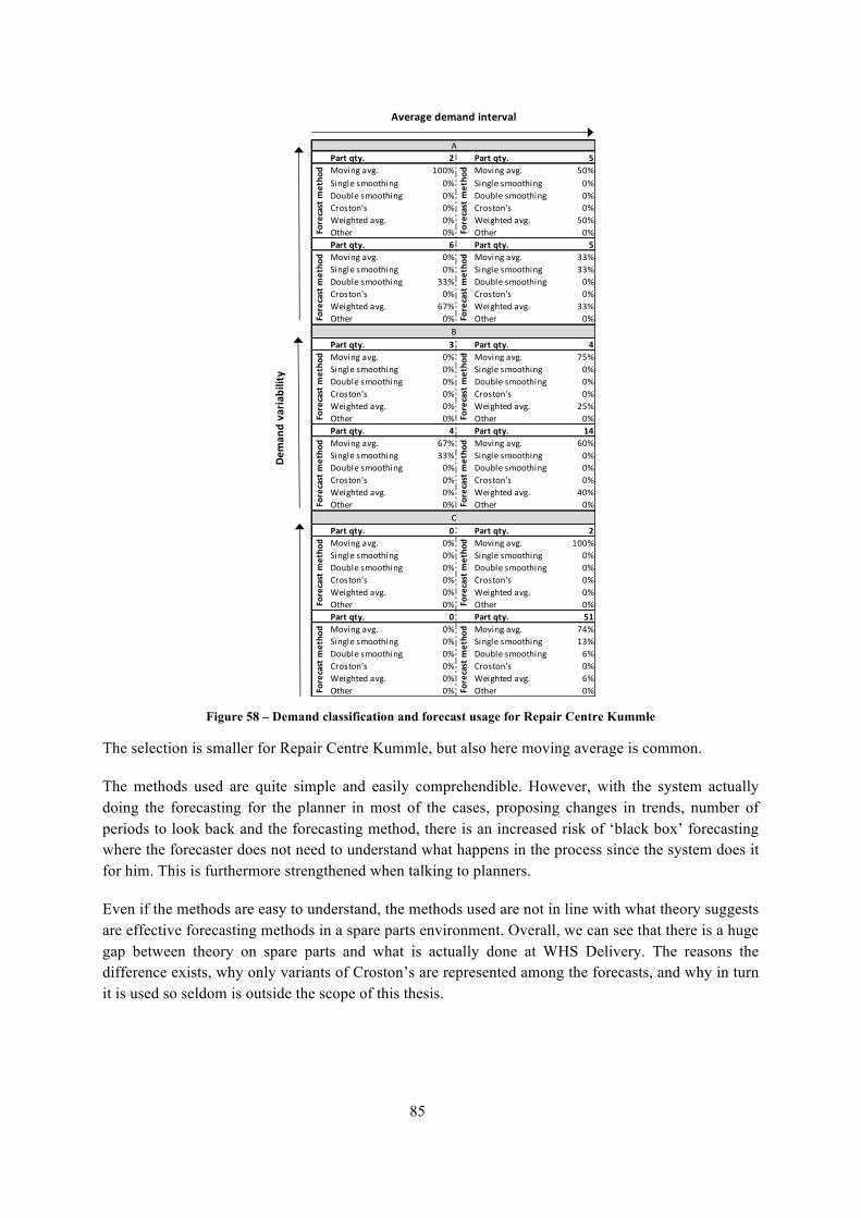
85

Figure 58 – Demand classification and forecast usage for Repair Centre Kummle

The selection is smaller for Repair Centre Kummle, but also here moving average is common.

The methods used are quite simple and easily comprehendible. However, with the system actually doing the forecasting for the planner in most of the cases, proposing changes in trends, number of periods to look back and the forecasting method, there is an increased risk of ‘black box’ forecasting where the forecaster does not need to understand what happens in the process since the system does it for him. This is furthermore strengthened when talking to planners.

Even if the methods are easy to understand, the methods used are not in line with what theory suggests are effective forecasting methods in a spare parts environment. Overall, we can see that there is a huge gap between theory on spare parts and what is actually done at WHS Delivery. The reasons the difference exists, why only variants of Croston’s are represented among the forecasts, and why in turn it is used so seldom is outside the scope of this thesis.

Part qty. 2 Part qty. 5Moving avg. 100% Moving avg. 50%Single smoothing 0% Single smoothing 0%Double smoothing 0% Double smoothing 0%Croston's 0% Croston's 0%Weighted avg. 0% Weighted avg. 50%Other 0% Other 0%Part qty. 6 Part qty. 5Moving avg. 0% Moving avg. 33%Single smoothing 0% Single smoothing 33%Double smoothing 33% Double smoothing 0%Croston's 0% Croston's 0%Weighted avg. 67% Weighted avg. 33%Other 0% Other 0%



Average demand interval

Forecast m

etho

d

Forecast m

etho

d

Forecast m

etho

d

Forecast m

etho

d

Forecast m

etho

d

Forecast m

etho

d

Forecast m

etho

d

A

B

C

Deman

d varia

bility

Forecast m

etho

d

Forecast m

etho

d

Forecast m

etho

d

Forecast m

etho

d

Forecast m

etho

d

86

6.5.6 FORECASTING IT-SYSTEMS

Based on the empirical data collection, the conclusion is that the forecasting is predominately in stage 1 in Mentzer et al. (1999) framework with some elements of stage 2 and stage 3, see Figure 59.

Figure 59 – Assessment of the forecasting IT-systems. Wireless Solutions compared to Mentzer et al. (1999)

The system is an integrated product for planning which also includes a forecasting application. Since it is not without flaws, the planner has to be alert to notice them which require training and experience. The system’s forecasting level of flexibility is low as it only allows the planner to forecast based on historic demand which leads to several factors left out of the forecast which has to be artificially compensated for by the planner by manipulating the historical graphs, adjusting the trend dramatically or changing the forecasting method.

Today, the breaking point when stopping using the install base values is after three months, but the product lifecycle is generally much longer and the risk that a customer in that short time period changes its installed base could be considered slim. An alternative is to slowly phase out the ratio of how much the install base volume is used and how much the historical demand pattern is used in forecasting over a longer time period after today’s three month breaking point. With today’s system this is not possible, but can be a more proper way of forecasting based on different data input. FAME is today a time-efficient tool for the Vendor Delivery Manager compared to older ways of working. It would benefit from a forecast accuracy calculation, in accordance with established theory and the audit.

Inventory Turnover changes and system adaptation

Xelus proposes recommendations which, if followed without consideration, would lead to overstock compared to the goals put forth regarding Inventory Turnover. When the Target Stock Levels are decreased in accordance with the Inventory Turnover goals, it is not communicated to the Repair Centres. Moreover, as Inventory Turnover has been increasing steadily during the last years, the Target Stock Levels are reduced leading to a reduced need for sourcing of new buy and repair. The planned and actual increases of Inventory Turnover are not taken into account in the forecasts which leads to baselines which might be too high. Moreover, it would be advantageous with continuous improvements of the system through reports of faults it makes, so developers can improve over time.

87

6.5.7 FORECASTING PERFORMANCE MEASUREMENTS

Based on the empirical data collection, the conclusion is that the forecasting related to performance measurements is in stage 1 in Mentzer et al. (1999) framework, as illustrated in Figure 60.

Figure 60 – Assessment of the forecasting performance measurements. Wireless Solutions compared to Mentzer et al.

(1999)

The authors agree with Van Dueren den Hollander (2014) that measuring is the first step in starting to improve the forecasting, which also is supported by theory as well (Moon et al., 1998).

Deciding on an aligned way of measuring

Measuring is scattered and there is no universal way that has been unanimously been agreed upon. The system makes forecasts based on due dates when parts are expected back at the L2, but the Repair Centres have their own way of measuring forecast accuracy which is measured like:

𝐹𝑜𝑟𝑒𝑐𝑎𝑠𝑡! = 𝐼𝑛𝑏𝑜𝑢𝑛𝑑 𝑑𝑒𝑙𝑖𝑣𝑒𝑟𝑖𝑒𝑠 𝑡𝑜 𝑅𝑒𝑝𝑎𝑖𝑟 𝐶𝑒𝑛𝑡𝑟𝑒! (6.12)

It can be argued that it is easier for the Repair Centres to change their way of measuring forecast accuracy than changing the software itself. If it is assumed that the RMA is created 28 days before the due date (for an E2E TAT of 28 calendar days), then the measurement for the Repair Centre would in that case look like (compared to the one used now):

𝐹𝑜𝑟𝑒𝑐𝑎𝑠𝑡! = 𝐼𝑛𝑏𝑜𝑢𝑛𝑑 𝑑𝑒𝑙𝑖𝑣𝑒𝑟𝑖𝑒𝑠 𝑡𝑜 𝑅𝑒𝑝𝑎𝑖𝑟 𝐶𝑒𝑛𝑡𝑟𝑒(!!!" !"#$%&"' !"#$) (6.13)

The new measurement is designed like this because if the RMA is created 28 days before the due date, the picking/packing at L2 takes 1 calendar day, the RMA request takes 1 calendar day and the shipping takes approx. 2 calendar days resulting in arrival at the Repair Centres 24 days before the due date (for Repair Centre Betamax and shipments from the L2 in Eindhoven). For other Repair Centres with different internal TAT and transportation lead-times there will be other another figure based on the same logic which can be applied to align the views of the forecasts. Looking at this new measurement, it becomes apparent that the forecasting measurement using inbound volumes are almost one month ahead of time. When the Monthly Business Review meeting is held in the middle of the month for discussing baseline for the upcoming month, products with due dates for that month has already started coming in to the Repair Centre. With stable volumes this would not matter greatly (albeit still being suboptimal), but as has been stated, the volumes are decreasing and can be unpredictable which leads to a potentially large mismatch between the expectations by the actors.

88

It is also important for the Repair Centres to understand that the planning tool only recognises the demand in monthly buckets, and not in weekly meaning that all parts for a month can arrive in the same week and the measurement figures on baseline accuracy would still be within the accepted interval. Planning in weekly buckets instead of monthly might be a desirable way of working, but as there are large forecast accuracy issues already, planning in weekly might be a premature idea. It is however important that the planners understand importance of continuity of work orders for the Repair Centres, especially for those that have challenges with downwards volume flexibility like Repair Centre Betamax.

Forecast accuracy and forecast deviation

Based on theory, Van Dueren den Hollander (2014), and the fact that there already is a proposal for implementation of forecast accuracy measurements for the FAME tool, that is a suitable start for measuring the forecast accuracy and deviation. When there is enough data to understand how the Repair Centres are affected by inaccurate forecasts, there should be some form of incentive system as well to provide accurate forecasts. Deciding on the most effective measurement system is outside the scope of this thesis, as there is already a detailed proposal for this.

Inventory Turnover

Not measuring the Inventory Turnover at the L3s and L4s locations can induce a risk of behaviour from planners where they choose to locate more stock than necessary at those locations. The introduction of measuring L3s and L4s locations later during 2014 is a step to reduce this risk.

Manual adjustments

Manual adjustments are used and in accordance with Armstrong (1987) and Van Dueren den Hollander (2014), when they are used, it should be explicitly stated. A record should be kept of the size of the adjustment and of the forecast accuracy with and without the adjustments to really start to see what the results of the adjustments are.

6.5.8 EXTENDED FRAMEWORK

Here the empirical data in relation to theory of the extension of framework created by Mentzer et al. (1999) is analysed.

Technical issues

The planners spend between 6-10 hours per month forecasting towards the Repair Centres (van Dueren der Hollander, 2014), which can be considered a short lead-time in this context and is not contingent on forecast horizon or the like.

For assumptions explicit, objective assessments can be gathered from Xelus, if not the past demand history has been manipulated in order to create a better forecast in the past. Understanding how well a specific forecasting method has performed during time, and questioning what the forecast bases its input on is important according to Armstrong (1987) and can help to question the output of it and by that propose an uncertainty estimation which can work as a guide for how much value you put into the forecast numbers.

89

Uncertainty estimation is not done today. When weighing the forecast and deciding the baseline it is more based on experience. It is somewhat done when seeing numbers that shoot off largely from the expected, but not in any structured way. Factors that could be deciding the uncertainty estimation can be previous forecast accuracy, average demand intervals, variation coefficient, and number of customers that has a contract with the GLSC. Another way of working can be to use objective methods to set upper and lower bounds for what forecast is considered to be surprising, and from that insight pay special focus to the outliers (Armstrong, 1987). Using subjective methods to set the upper and lower bounds are considered to be done with caution according to Armstrong (1987).

The forecaster and the users

The time series used are quite straightforward, lowering the requirements of the planners’ knowledge. Knowledge is a small help since it is often common with general trial and error when determining the right forecast method26. The planning tool is correct enough for the planner not to manually intervene in most of the cases. The functionality “auto forecast” can propose a completely new forecast which the software thinks are the most appropriate one based on the historical demand patterns, also changing the forecast method as well if appropriate. Furthermore, only a few are used and knowledge of the more complex ones is not demonstrated which can influence the choice of forecast method in the end.

Forecaster’s managerial style i.e. choice of forecasting method may affect the forecasting procedures adopted by the organisation. Furthermore, training affects these aspects as well. The training is done on the job, and the amount of training a new planner receives is dependent on the level of experience since before, which gives room for differentiation in the approach the planner has to planning, i.e. the style of the planner.

The assumption can then be that it is not structured. This can lead to that every individual develops a personal style when forecasting and planning which is validated from several sources in the organisation. As the software selects the most appropriate method in most cases, the managerial style of the forecaster is reduced related to selection of forecasting method. There are however other factors that are important to consider such as planner’s general style both when forecasting and planning. In the GSLC in China the planners put a lot of effort into the forecast and then in sending the same amount on a weekly basis towards the repair centres.

There are much manual work done and personal preference, time of the day, day of the week and other factors can play an important role, as the system allows a high degree of freedom in planning which definitely has an impact on the forecast accuracy. This is true for many types of jobs of course, but it is important to be aware of this aspect and counteract it with knowledge sharing and sharing of best practices.

Costs and benefits

Resources available encompass the resources spent into data search and collection in order to utilise the data into the forecasts. Data is automatically retrieved from the warehousing systems, and as historical data is the main input in the forecasting, not so much resources are put into gathering of data today.

26 Kevin Kusters, interview the 29th of April, 2014

91

7 DISCUSSION The discussion chapter elaborates on the improvement strategies presented in the analysis chapter. The discussion is surrounding generalizability and barriers for change. Continuously the chapter also address possibilities for combination of the analysed improvement measures.

7.1 FORECASTING There are many identified ways to improve the forecasting accuracy of WHS Delivery, some easier to implement and some which requires more investment and time. Insight has been gathered from actors in the flows’ viewpoints of where there is room for potential. The insight combined with a solid theoretical frame of reference has acted as guidance in data collection. The final identified ways of improvement are based on theoretical knowledge of how forecasting can be improved in industrial settings, but the actual improvements are to some extent suited to the context of Wireless Solutions. As Wireless Solutions is low on all four pillars of Mentzer et al. (1999), there are more possibilities for further work after the initial improvements have been made. A new scan of the four dimensions can reveal new insights into where the next steps are to put focus into. The framework used in this study is designed for forecasting in general, and not for an aftermarket which can potentially have negative effect. However, the activities of forecasting do not really change but the demand characteristics, which indeed are taken into consideration. Therefore, using the framework of Mentzer et al. (1999) is feasible in this context.

One part of the purpose of this master thesis was to reduce the supply chain related costs by improving forecasting. The initial ambition was to show how much the costs can be reduced, and how much it would cost to actually reduce the forecast errors. However, while identifying ways of improving the performance, it was realised that it was hard to quantify firstly how much the forecasting performance can be improved by the proposed actions, and secondly the costs associated with implementation of the changes. Some changes are naturally less costly to implement and are more costly. The thesis however has provided an estimation of the costs the forecast errors contributes to, and from that cost-saving potential, the actions should be evaluated.

7.1.1 GENERALIZABILITY

New ways of working cannot solely be based on improved forecast accuracy towards one Repair Centre, but towards all Repair Centres globally which leads to a much higher potential. Adopting new ways of working towards all Repair Centres on a global scale is facilitated by having the material planners relatively centralised in the GSLCs, the planning software centralised, which both decrease the costs of implementation of new routines and applications. However, the actions taken should be based on a sound business sense of the potential benefits compared to the costs and associated risks. Picking the “low hanging fruit” is a start, and can be done without incurring higher costs operationally.

7.1.2 BARRIERS FOR CHANGE

Barriers for change include the fact that the stakeholders which has the mandate to drive change is not directly in the part of the organisation that directly benefits of an improved forecast. The benefits are most noticeably experienced at the suppliers’, e.g. internal and external Repair Centres, internal supply sites where new-buy is purchased and Logistics Service Providers like CEVA and TNT. In the end,

92

the effects are going to be clear also for the GSLC and Customer Units with the result of lower prices from their suppliers, better delivery precision and in the end more satisfied customers. The stakeholders with the ability to make changes therefore needs to be dedicated to the project, understand and believe in the potential and do what is needed to drive change in the organisation with regards to forecasting. In order to gain attention, the extra costs created with can be attributed to forecasting accuracy should be explicitly stated, hopefully this report has succeeded in doing so to gain a first awareness of the problems.

7.2 STRATEGIES FOR VARIATION REDUCTION The most cost-efficient way of the strategies for variation reduction is the OOLT concept where faulty and good parts are kept at the L2 with a call-off mechanism to receive just the right amount of units every week for the Repair Centres. A thorough comparison through simulation has been made between the different alternatives which strengthens the reliability. Moreover, a few assumptions are made and the outcome is contingent on those.

7.2.1 GENERALIZABILITY

The analysis has shown the potential and set-up for Repair Centre Betamax, but applying this way of working on all Repair Centres is not feasible without preparations with a business case. Some Repair Centres have the potential to even out the volumes of inbound faulty stock with other activities reducing the costs associated to the variation of inbound faulty repair. However, OOLT might be suitable in several cases since there are not large investments when keeping the stock located at the L2.

When the smoothing of the variation is dependent on quick replenishments from the L2s, transportation time also becomes a factor. The solutions might be suitable where transportation lead-time is short and transports do not risk being lost and the risk of delay is reduced. If transportation lead-time between the L2 and Repair Centre is longer, a portion of the faulty stock can be used as a buffer stock at the Repair Centres.

The idea might not be suitable for NPI products due to the fact that the demand of the products often increase every month making it challenging to level within months and anticipate the increases. Moreover, the faulty stocks can often be lower for NPI products because enough parts have not yet been faulty, or the faulty parts might not yet have been delivered back to the L2. These aspects also decrease the possibilities to level the production through OOLT or the combination of MTS and MTO. For EOL products, there is the ever-present risk to build stock that there never will be a demand for.

Using OOLT in environments where the forecast is notoriously wrong might be risky since the OOLT’s are calculated based on forecast. Instead the segmentation strategy can be combined with the OOLT concept which would result in only A-parts with the characteristics as “smooth” can be placed as an OOLT.

7.2.2 REDUCTION OF CAPACITY

Potential for capacity reductions is dependent on the volumes of the parts being analysed or repaired in a specific machine, and the diverseness of the machines within the product group. IIn the case of Repair Centre Betamax, it was only possible to reduce the capacity for the high runner product group,

93

URA2. For all other product groups, due to a low number of machines and/or a diverseness of the machines handling the parts within the product groups, a levelled flow could not reduce capacity. Considering Repair Centre Betamax being one of the larger Repair Centres, and the URA2 product group represents over half of the volume, it strengthens the argument that NPI Repair Centres might not stand to benefit as much from this concept.

7.2.3 BARRIERS FOR CHANGE

Even if the business case clearly shows a large potential cost savings potential in implementing OOLT with the placement of faulty stock at the L2, structural challenges remain. The KPI Inventory Turnover is very relevant today for WHS Delivery, and any sign that the value has the potential to be decreased can create larger resistance than larger cost savings in the flow as a whole. Discussions have been held regarding who shall have the repaired good stock before the due date where it is argued from a Material Management point of view that the good stock shall be back at the L2 on the due date (which is not the case today), but with a new way of working the good stock will in many cases be back at the L2 long before the due date – either in the Repair Centre ownership or in the GLSC ownership. Having the parts back in the GSLC ownership reduces ITO, but keeping it in the Repair Centre ownership can potentially reduce delivery performance to customers. The good stock repaired before the due date shall be used to its fullest potential, and finding a way to do so remains a challenge even after implementation. One option could be to keep a small good stock at the L2 for which Betamax carries the cost and GSLC can use those parts to meet customers’ demand.

7.3 COMBINATION OF IMPROVEMENT STRATEGIES Giving the right opportunities for improving the forecasts is the first step. Also, realising that forecasting in a spare parts environment is difficult and that it can never be perfect is also important. This realisation means that there will always be a need to handle deviation of inbound volumes. The more the forecasting is improved, the less is the need for additional volumes to be used as a levelling mechanism. The OOLT concept in itself will never be as cost-efficient as improving the forecasting performance, excluding the investment costs in implementing since the OOLT concept is dependent on increasing the inventory levels of good stock while improving the forecasting is not. Furthermore, the concept is not as easily generalizable and requires more decentralised work and involvement of more functions and actors and is not as scalable, but it is important to see that for Repair Centre Betamax, it has a large cost savings potential compared to the extra costs incurred with a higher inventory level.

In other words, combining the recommendations from both business cases can work together to reduce capacity, costs and thereby the repair price and in the end increase customer satisfaction.

95

8 CONCLUSIONS & RECOMMENDATIONS The conclusions and recommendations chapter presents conclusion for the identified improvements of forecasting as well as the change of production strategy. In addition, concluding remarks of integrating the two improvement strategies are elaborated. The chapter continues with an outline of the recommendations to Wireless Solutions for future actions.

8.1 FORECASTING CONCLUSIONS Forecasting and planning is complex and depends on many different parameters which increases the difficulty of achieving high forecast accuracy. We have seen that there is a large cost saving potential in improving the forecast accuracy for Repair Centre Betamax making it worth looking into ways of improving the forecast performance.

A number of different angles and ways have been identified to improve the forecast performance at WHS Delivery. There are benefits to gain from working more with data from the installed base. Having a higher functional integration can lead to less duplication of forecasting efforts. Furthermore, being able to forecast based on more data inputs than historical demand can facilitate centralisation of forecasting efforts. The baseline procedure is not designed optimally in general and towards the internal Repair Centres in particular. The used forecasting methods are not aligned with theory, and the system used has room for improvement and should continuously be improved with feedback from its users. There is much needed improvement to be done with measurements, much in terms of alignment between the actors of definitions and ways of working. There are much room for personal style related to planning which increases the importance of educational efforts and best practice sharing between the planners to ensure effective forecasting and planning from the planners.

Improving forecasting has a high degree of generalizability and scalability but there are some barriers for change. Driving change is dependent on people who today do not stand the most to gain from improved forecast accuracy. There is a need of a holistic view on the organisation to identify the increased value created for the organisation with a cost reduction and or a price decrease for the end customer.

8.2 PRODUCTION STRATEGY CONCLUSIONS Variation of inbound repair volumes incurs costs mostly when volumes deviate downwards under 80% of the baseline. Using a buffer of parts before repair, it is possible to reduce the supply chain costs within the WHS Repair Logistics Flow. The reduced costs can mostly be attributed to reduced asset costs and to some extent reduce costs for blue collar salaries. An introduced buffer however affects GSLC through a higher inventory level and potentially more administrative tasks.

Two different buffer approaches to levelling have been compared. Using a combination of MTO and MTS where MTS is used for parts with smooth and high demand can work as a levelling plan, but the approach is complex with a lower level of generalizability and economically not as a cost-efficient solution as the OOLT alternative. This approach leads to a reduction of 3% of the supply chain costs when levelling the production to +-20%. For maximizing the asset utilisation in a specific high volume product flow however, this approach is more suitable at the smoothing volumes can be manually chosen. The second approach of using OOLT is less complex and associated with less uncertainty as it

96

has been used before in the WHS Repair Logistics Flow. This approach leads to a reduction of 5% of the supply chain costs when levelling the production to +-20%. Combining this approach while keeping the faulty parts at L2s however increases uncertainty as new relations potentially have to be formed.

Even if the proposed strategies are beneficial from a cost perspective, finding a way around the issue of conflicting KPI of ITO is still a challenge to be dealt with where defining the ownership of the parts after repair is the most pressing issue.

8.3 CONCLUDING REMARKS The thesis’ different approaches of reducing supply chain costs are interrelated as they both try to tackle the efficiency of the Repair Centres and reducing the delta between baseline and inbound deliveries of repair parts. The forecasting approach is however wider as it reaches outside the initial scope of repair forecasts and measures proposed can have an impact on the whole forecasting process in itself. In contrast, the use of buffer stock considers a more narrow approach. Combining the wide and narrow approach will contribute to strengthen the value proposition, increasing competitiveness on an uncertain aftermarket.

Improving forecasting has large room for reduction of supply chain costs and levelling the inbound flow of faulty parts to Repair Centres can reduce the supply chain as well, leading to fulfilment of the purpose of the thesis.

8.4 RECOMMENDATIONS This section describes the recommendations for Wireless Solutions for reducing supply chain costs through improving the forecast and levelling the repair operations at Repair Centre Betamax.

8.4.1 FORECASTING

The way forward regarding forecasting differs depending on the time frame. Something that always can applied however to gain further insights and ideas for improvement is to use theory to improve forecasting. More concrete recommendations are expressed based on short, medium and long term actions.

Short term • Make the personnel connected to the forecasting aware of the impact of inaccurate forecasts. • Change baseline procedure for internal Repair Centres • Align measurements of forecast accuracy between Repair Centre and GSLC • Investigate forecasting methods usage • Increase information sharing to avoid miscommunication and late reactions at RC

o Set up communication platform between GSLC and Vendors • Investigate using other input, not only historical data • Try to gauge and explore what the best practices are for planners both holistically and on the

specific points o Delivery precision o Repair cost

97

o Inventory Turnover • Call for knowledge sharing within planning • Understand which parts are the hardest to plan for (lumpy parts)

Medium term (6 months – 1 year) • Investigate possibility to include incentive for customers to report installed base figures

Long term (1 year – 3 years) • Pilot test of using installed base figures

8.4.2 PRODUCTION STRATEGY

• OOLT can be implemented quite quickly due to no strict warehouse space limitations • Begin discussions with CEVA Logistics regarding the concept of changed working routines

and gain understanding of how they perceive the situation

8.4.3 COMBINED RECOMMENDATIONS

Improving the forecasting as well as introducing the OOLT concept for Repair Centre Betamax should be considered parallel activities where they both can work synergistically.

99

9 REFERENCES Alicke, K. (2003) Planung und Betrieb von Logistiknetzwerken. Heidelberg: Springer.

Altay, N. (2011) Service Parts Management – Demand Forecasting and Inventory Control. London: Springer-Verlag ISBN 978-0-85729-038-0

Armstrong, J. S. (1987) The forecasting audit. In: Makridakis & Wheelwright, S. C., The handbook of forecasting. New York: John Wiley, pp. 584–602.

Ayers, J. B. (2001) Handbook of Supply Chain Management. St. Lucie Press/APICS: Boca Raton, Fla. ISBN: 978-1-4665-1005-0.

Bacchetti, A. and Saccani, N. (2012) Spare parts classification and demand forecasting for stock control: Investigating the gap between research and practice, Special Issue on Forecasting in Management Science, vol. 40, iss. 6, pp. 722-737.

Ballou, R. H. (1973) Business logistics management. Englewood Cliffs, N. J.: Prentice-Hall

Bickman, L. and Rog, D. J. (1998) Handbook of Applied Social Research Methods, Sage Publications, Thousand Oaks, CA.

Boxersox, D., Closs, D. and Cooper, M. B. (2009) London: McGraw-Hill Higher Education.

Boylan J. E. and Syntetos, A. A. (2008) Forecasting for Inventory Management of Service Parts. Chapter 20 in: Complex System Maintenance Handbook, pp. 479-506.

Boylan, J. E and Syntetos, A. A. (2009) Spare parts management: a review of forecasting research and extensions. IMA Journal of Management Mathematics, vol. 21, iss. 21, pp. 227–237.

Boylan, J. E., Syntetos, A. A. and Karakostas, G. C. (2008) Classification for forecasting and stock control: a case study, Journal of Operational Research Society, vol. 59, iss. 4, pp. 473-481.

Bryman, A. and Bell, E. (2003) Business research methods. Oxford University Press.

Bucher, D. and Meissner, J. (2011) Configuring Single-Echelon Systems Using Demand Categorization. in: Service Parts management – Demand Forecasting and Inventory Control, pp. 203-219.

Byrne, P. J and Heavey, C. (2006) The impact of information sharing and forecasting in capacitated industrial supply chains: A case study. International Journal of Production Economics, vol. 103, iss. 1, pp. 420-437.

Cavalieri, S., Macchi, M., Garetti, M., Pinto, R. (2008) A decision making framework for spare parts inventory planning: proposal and validation in industrial cases. Production Planning Control, vol. 19, iss 4, pp. 379–396.

100

Chakraborty, T., Chauhan, S. S. and Giri, B. C. (2013) Joint effect of stock threshold level and production policy on an unreliable production environment. Applied Mathematical Modelling, vol. 37, iss. 10-11, pp. 6593.

Chen J. (1997) Achieving maximum Supply chain efficiency, IIE Solutions, vol. 29, iss. 6, pp. 30-35.

Chopra, S and Meindl, P. (2012) Supply chain management: Strategy, Planning and Operation. 5th

Edition. Essex, England: Pearson Education Limited 5th Edition

Christopher, M. and Towill, D.R. (2001) An integrated model for the design of agile supply chains. International Journal of Physical Distribution & Logistics Management, vol. 31 iss. 4, pp. 235-246.

Cohen M. A., Agrawal N. and Agrawal, V. (2006) Winning in the aftermarket. Harvard Business Review, vol. 1, no. 84, pp. 129–138.

Croston, J. D. (1972) Forecasting and stock control for intermittent demands. Operational Research Quarterly, vol. 23, iss. 3, pp. 289-303.

Deloitte (2011) Driving profitability through aftermarket parts pricing [online publication]. Available at: https://www.deloitte.com [2014-05-26]

Ejvegård, R. (2009) Vetenskaplig metod. 4th edition. Lund: Student literature.

Fahmy Salama, K., Luzzatto, D., Sianesi, A. and Towill, D. R. (2009) International Journal of Production Economics, International Journal of Production Economics, vol. 119, iss. 1, pp. 34-45, ISSN 0925-5273.

Fildes, R. and Hastings, R. (1994) The organization and improvement of market forecasting. Journal of the operations research society, vol. 45, iss. 1, pp. 1-16.

Fisher, M.L. (1997) What is the right supply chain for your product?, Harvard Business Review, vol. 75 iss. 2, pp. 105-116.

Flores, B. E. and Whybark, D. C. (1986) Multiple Criteria ABC Analysis, International Journal of Operations & Production Management, vol. 6, iss. 3, pp. 38-46.

Ghali, M. A. (1993) Models of production and inventory behaviour, Economic Modelling, vol. 10, iss. 1, pp. 57-63.

Ghobbar, A. A. and Friend, C. H. (2002) Sources of intermittent demand for aircraft spare parts within airline operations. Journal of Air Transport Management, vol. 8, iss. 4, pp. 221-231.

Glueck, J. J., Koudal, P. and Vaessen, W. (2006) The service revolution [online publication]. Available at: https://www.deloitte.com [2014-05-26]

Goldsby, T.J., Griffis, S.E. and Roath, A.S. (2006), Modeling lean, agile, and leagile supply chain strategies. Journal of Business Logistics, vol. 27 no. 1, pp. 57-80.

101

Golicic S. L., Davis D. F. and McCarthy T. M. (2005) A Balanced Approach to Research in Supply Chain Management. in: Kotzab, H and Westhaus, M (2005) Research methodologies in supply chain management. Heidelberg: Physica.

Guba, E. G. (1981) Annual Review Paper: Criteria for assessing the trustworthiness of naturalistic inquiries, Educational Communication and Technoindoorlogy, vol. 29, iss. 2 (Summer, 1981), pp. 75-91.

Hill, T. (1993) Manufacturing Strategy: Text and Cases. 2nd edition. London: Macmillan.

Huber, A. J. (2011) Common mistakes and guidelines for change in service parts management. Chapter 14 in: Service Parts management – Demand Forecasting and Inventory Control, pp. 279-307.

Jacobs, R. F., Williams L. B., Whybark, D. C. and Vollman, T. E. (2011) Manufacturing planning and control. 6th edition. New York: McGraw-Hill. ISBN 978-007-132518-9

Jacobsen, D. I. (2002) Vad, hur och varför, om metodval företagsekonomi och andra samhällsvetenskapliga ämnen. Lund: Studentlitteratur AB.

Johansson, H. J., Mchugh, P., Pendlebury, A. J. and Wheeler, W. A. (1993) Business Process Re-engineering: Breakpoint Strategies for Market Dominance. Chichester, UK: Wiley.

Johnston, F. R. and Boylan, J. E. (1996) Forecasting for items with intermittent demand. Journal of Operational Research Society, vol. 47, iss. 1, pp. 113-121.

Jonsson, P. and Mattsson, S. A. (2009) Manufacturing planning and control, London: Mcgraw-Hill Education.

Kalchschmidt, M (2012) Best practices in demand forecasting: Tests of universalistic, contingency and configurational theories. International journal of production economics, vol. 140, iss. 2, pp. 782-793.

Kothari, C. R. (2004) Methodology, Methods and Techniques. New Delhi, India: New age international (P) Limited

Kotzab, H. and Westhaus, M. (2005) Research methodologies in supply chain management. Heidelberg: Physica.

Krishnaswamy, O. R. and Satyaprasad, B. G. (2010) Business research methods. Himalaya Pub. House

Kumar, R. (2011) Research methodology, a step-by-step guide for beginners. London: Sage Publications.

Lambert, D. M. (1976) The development of an inventory costing methodology: a study of the costs associated with holding inventory. Chicago: National council of physical distribution management.

Lambert, D. M. and Cooper, M. (2000) Issues in Supply Chain Management, Industrial Marketing Management, vol. 29, iss. 1, pp. 65-83.

102

Lambert, D. M., Stock, J. R. and Ellram, L (1998) Fundamentals of logistics management. New York: McGraw-Hill Publishing Co.

Lewis, H. T., Culiton, W. and Steele, J. D. (1956) The role of airfreight in physical distribution. Boston, MA: Harvard Business Review.

Liker, J and Meier, D. (2006) The Toyota Way Fieldbook. New York: Mcgraw-Hill Companies

Lo, M.S. and Power, D. (2010) An empirical investigation of the relationship between product nature and supply chain strategy. Supply Chain Management: An International Journal, vol. 15, iss. 2, pp. 139-153.

Lumsden, K. (2006) Logistikens grunder, Studentlitteratur, Lund.

Macchi, L. L., Fumagalli, R. Pinto, R. and Cavalieri, S. (2011) A Decision Making Framework for Managing Maintenance Spare Parts in Case of Lumpy Demand: Action Research in the Avionic Sector. Chapter 9 in: Service Parts management – Demand Forecasting and Inventory Control, pp. 171-202.

MacDonnell, M. and Clegg, B. (2011) A New Inventory Model for Aircraft Spares. Chapter 7 in: Service Parts management – Demand Forecasting and Inventory Control, pp. 143-156.

Mason-Jones, R., Naylor, B. and Towill, D.R. (2000) Engineering the leagile supply chain. International Journal of Agile Management Systems, vol. 2, iss. 1, pp. 54-61.

Mentzer, J. T., Bienstock, C. C. and Kahn, K. B. (1999) Benchmarking sales forecasting management, vol. 42, iss. 3, pp. 48-56.

Minner, S. (2011) Forecasting and Inventory Management for Spare Parts: An Installed Base Approach. Chapter 8 in: Service Parts management – Demand Forecasting and Inventory Control, pp. 157-169.

Minnich and Maier (2006) Supply Chain Responsiveness and Efficiency: Complementing Or Contradicting Each Other? 24th International Conference of the System Dynamics Society, Nijmegen 2006b, pp. 1–16.

Mollenkopf, D., Russo, I. and Frankel, R. (2007) The returns management process in supply chain strategy (2007), International Journal of Physical Distribution & Logistics Management, vol. 37, iss. 7, pp. 568-592.

Moon, M. A., Mentzer, J. T. and Smith, C. D. (2003) Conducting a sales forecasting audit. International journal of forecasting, vol. 19, iss. 1, pp. 5-25.

Moon, M. A., Mentzer, J. T., Smith, C. D. & Garver, M. S. (1998) Seven keys to better forecasting. Business Horizons, vol. 41, iss. 5, pp. 44-52.

Murthy, D. N. P., Solem, O., and Roren T. (2004) Product warranty logistics: Issues and challenges, European Journal of Operations Research, vol. 156, iss. 1, pp. 110–126.

103

Naim, M., Childerhouse, P., Disney, S. and Towill, D. (2002) A supply chain diagnostic methodology: determining the vector of change. Computers & Industrial Engineering, vol. 43, iss. 1-2, pp. 135–157, ISSN 0360-8352

Naylor, J.B., Naim, M.M. and Berry, D. (1999) Leagility: integrating the lean and agile manufacturing paradigms in the total supply chain”, International Journal of Production Economics, vol. 62, iss 1-2, pp. 107-118.

Olhager, J (2010) Produktionsekonomi. Lund: Studentlitteratur.

Oskarsson, B. Aronsson, H and Ekdahl, B. (2013) Modern logistik – för ökad lönsamhet. 4th edition, Malmö: Liber.

Patel, R. and Davidson, B. (2011) Forskningsmetodikens grunder. Att planera, genomföra och rapportera en undersökning. 4th edition, Lund: Student literature.

Pettesson, A. I. and Segerstedt, A (2013) Measuring supply chain costs, International Journal of Production Economics, vol. 143, iss. 2, pp. 357-363.

Sachan, A., Sahay, B. S. & Sharma, D. (2005) Developing Indian grain Supply chain cost model: system dynamics approach, International Journal of Productivity and Performance Management, vol. 54, iss. 3, pp. 187-205.

Sachdeva, J. K. (2009) Business Research Methodology. Mumbai: Global Media.

Scholtz, R. W. and Tietje, O. (2002) Embedded Case Study Methods. Thousand Oaks, USA: Sage Publications.

Schultz, R. (1992). Fundamental aspects of forecasting in organisations. International Journal of Forecasting, vol. 7, iss. 4, pp. 409–411.

Srivastava, S. K. (2012) Growing importance of reversed logistics. Cargoconnect, March.

Stratton, R. and Warburton, R.D.H. (2003) The strategic integration of agile and lean supply, International Journal of Production Economics, vol. 85, no. 2, pp. 183-198.

Syntetos A. A. and Boylan J. E. (2001) On the bias of intermittent demand estimates. International Journal of Production Economy, vol. 71, iss. 1-3, pp. 457-466.

Syntetos, A. A., Boylan, J. E. Croston, J. D. (2005) On the categorization of demand patterns. Journal of Operational Research Society, vol. 56, iss. 5, pp. 495-503.

Teunter, R. (2008) Intermittent demand forecasting & control. Lancaster University Management School

Van Dueren den Hollander, P. (2014) Supply Chain Management – Forecasting of spare parts within Wireless Solutions. Breda: TiasNimbas – MOS2.

104

Yin, R. K. (2009) Case Study Research: design and methods. 4th edition, Thousand Oaks, USA: Sage Publications.

105

10 APPENDICES

10.1 THROUGHPUT TIME The process is mapped taking into consideration material, information and the costs associated with supply chain related activities.

𝑆𝑡𝑜𝑟𝑎𝑔𝑒 𝑙𝑒𝑎𝑑 𝑡𝑖𝑚𝑒 = 12 𝑑𝑎𝑦𝑠 + 93 𝑑𝑎𝑦𝑠 + 16 𝑑𝑎𝑦𝑠 + 60 𝑑𝑎𝑦𝑠 = 181 𝑑𝑎𝑦𝑠 (10.1)

The storage lead-time includes storage at customer unit, L2, repair centre and L2 again. If the scope would expand to cover good stock at L3, L4 and L5, the storage lead-time would increase.

𝑇𝑟𝑎𝑛𝑠𝑝𝑜𝑟𝑡 𝑙𝑒𝑎𝑑 𝑡𝑖𝑚𝑒 = 2 𝑑𝑎𝑦𝑠 + 2 𝑑𝑎𝑦𝑠 + 2 𝑑𝑎𝑦𝑠 = 6 𝑑𝑎𝑦𝑠 (10.2)

The calculations are done for the most common case, but it can happen that the transportation time is increased to up to 10 days in total.

𝑇𝑟𝑜𝑢𝑏𝑙𝑒𝑠ℎ𝑜𝑜𝑡𝑖𝑛𝑔 𝑎𝑛𝑑 𝑟𝑒𝑝𝑎𝑖𝑟 𝑙𝑒𝑎𝑑 𝑡𝑖𝑚𝑒 = ~0.07 𝑑𝑎𝑦𝑠 (10.3)

The trouble shooting and repair lead-time is based on the average time it takes for these activities at Repair Centre Betamax.

𝑇ℎ𝑟𝑜𝑢𝑔ℎ𝑝𝑢𝑡 𝑡𝑖𝑚𝑒 =𝑆𝑡𝑜𝑟𝑎𝑔𝑒 𝑙𝑒𝑎𝑑 𝑡𝑖𝑚𝑒 + 𝑇𝑟𝑎𝑛𝑠𝑝𝑜𝑟𝑡 𝑙𝑒𝑎𝑑 𝑡𝑖𝑚𝑒 + 𝑡𝑟𝑜𝑢𝑏𝑙𝑒𝑠ℎ𝑜𝑜𝑡𝑖𝑛𝑔 𝑎𝑛𝑑 𝑟𝑒𝑝𝑎𝑖𝑟 𝑙𝑒𝑎𝑑 𝑡𝑖𝑚𝑒 =

181 𝑑𝑎𝑦𝑠 + 6 𝑑𝑎𝑦𝑠 + 0.07 𝑑𝑎𝑦𝑠 = 187.07 (10.4)

𝑉𝑎𝑙𝑢𝑒 𝑎𝑑𝑑𝑒𝑑 𝑡𝑖𝑚𝑒𝑇ℎ𝑟𝑜𝑢𝑔ℎ𝑝𝑢𝑡 𝑡𝑖𝑚𝑒

=0.07 𝑑𝑎𝑦𝑠187.07 𝑑𝑎𝑦𝑠

= 3.7×10!!% = 0.037% (10.5)

As can be seen, the actual value added time for a general service unit going through the flow, is very short compared to the throughput time.

Supply chain cost reduction - Chalmers Publication Library...

Documents

Transcript of Supply chain cost reduction - Chalmers Publication Library...