Supplementary Material: Multiple Texture Boltzmann...
3
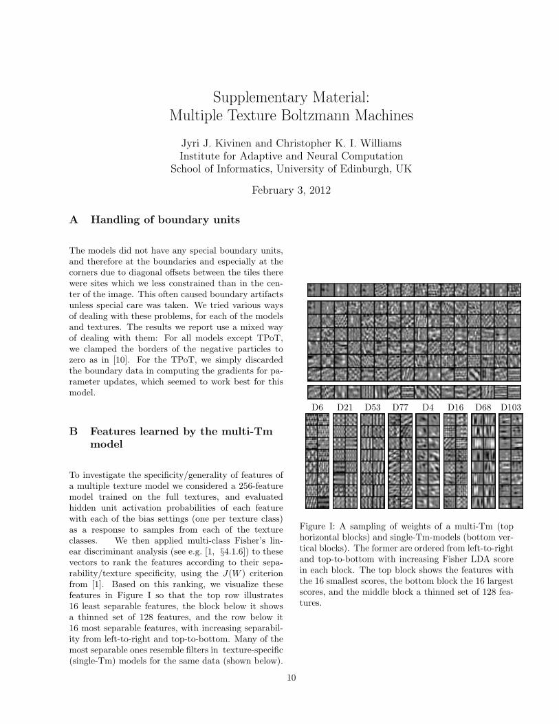
Supplementary Material: Multiple Texture Boltzmann Machines Jyri J. Kivinen and Christopher K. I. Williams Institute for Adaptive and Neural Computation School of Informatics, University of Edinburgh, UK February 3, 2012 A Handling of boundary units The models did not have any special boundary units, and therefore at the boundaries and especially at the corners due to diagonal offsets between the tiles there were sites which we less constrained than in the cen- ter of the image. This often caused boundary artifacts unless special care was taken. We tried various ways of dealing with these problems, for each of the models and textures. The results we report use a mixed way of dealing with them: For all models except TPoT, we clamped the borders of the negative particles to zero as in [10]. For the TPoT, we simply discarded the boundary data in computing the gradients for pa- rameter updates, which seemed to work best for this model. B Features learned by the multi-Tm model To investigate the specificity/generality of features of a multiple texture model we considered a 256-feature model trained on the full textures, and evaluated hidden unit activation probabilities of each feature with each of the bias settings (one per texture class) as a response to samples from each of the texture classes. We then applied multi-class Fisher’s lin- ear discriminant analysis (see e.g. [1, §4.1.6]) to these vectors to rank the features according to their sepa- rability/texture specificity, using the J (W ) criterion from [1]. Based on this ranking, we visualize these features in Figure I so that the top row illustrates 16 least separable features, the block below it shows a thinned set of 128 features, and the row below it 16 most separable features, with increasing separabil- ity from left-to-right and top-to-bottom. Many of the most separable ones resemble filters in texture-specific (single-Tm) models for the same data (shown below). D6 D21 D53 D77 D4 D16 D68 D103 Figure I: A sampling of weights of a multi-Tm (top horizontal blocks) and single-Tm-models (bottom ver- tical blocks). The former are ordered from left-to-right and top-to-bottom with increasing Fisher LDA score in each block. The top block shows the features with the 16 smallest scores, the bottom block the 16 largest scores, and the middle block a thinned set of 128 fea- tures. 10
-
Upload
phunghuong -
Category
Documents
-
view
230 -
download
0
Transcript of Supplementary Material: Multiple Texture Boltzmann...
Supplementary Material:Multiple Texture Boltzmann Machines
Jyri J. Kivinen and Christopher K. I. WilliamsInstitute for Adaptive and Neural Computation
School of Informatics, University of Edinburgh, UK
February 3, 2012
A Handling of boundary units
The models did not have any special boundary units,and therefore at the boundaries and especially at thecorners due to diagonal offsets between the tiles therewere sites which we less constrained than in the cen-ter of the image. This often caused boundary artifactsunless special care was taken. We tried various waysof dealing with these problems, for each of the modelsand textures. The results we report use a mixed wayof dealing with them: For all models except TPoT,we clamped the borders of the negative particles tozero as in [10]. For the TPoT, we simply discardedthe boundary data in computing the gradients for pa-rameter updates, which seemed to work best for thismodel.
B Features learned by the multi-Tmmodel
To investigate the specificity/generality of features ofa multiple texture model we considered a 256-featuremodel trained on the full textures, and evaluatedhidden unit activation probabilities of each featurewith each of the bias settings (one per texture class)as a response to samples from each of the textureclasses. We then applied multi-class Fisher’s lin-ear discriminant analysis (see e.g. [1, §4.1.6]) to thesevectors to rank the features according to their sepa-rability/texture specificity, using the J(W ) criterionfrom [1]. Based on this ranking, we visualize thesefeatures in Figure I so that the top row illustrates16 least separable features, the block below it showsa thinned set of 128 features, and the row below it16 most separable features, with increasing separabil-ity from left-to-right and top-to-bottom. Many of themost separable ones resemble filters in texture-specific(single-Tm) models for the same data (shown below).
D6 D21 D53 D77 D4 D16 D68 D103
Figure I: A sampling of weights of a multi-Tm (tophorizontal blocks) and single-Tm-models (bottom ver-tical blocks). The former are ordered from left-to-rightand top-to-bottom with increasing Fisher LDA scorein each block. The top block shows the features withthe 16 smallest scores, the bottom block the 16 largestscores, and the middle block a thinned set of 128 fea-tures.
10
Jyri J. Kivinen, Christopher K. I. Williams
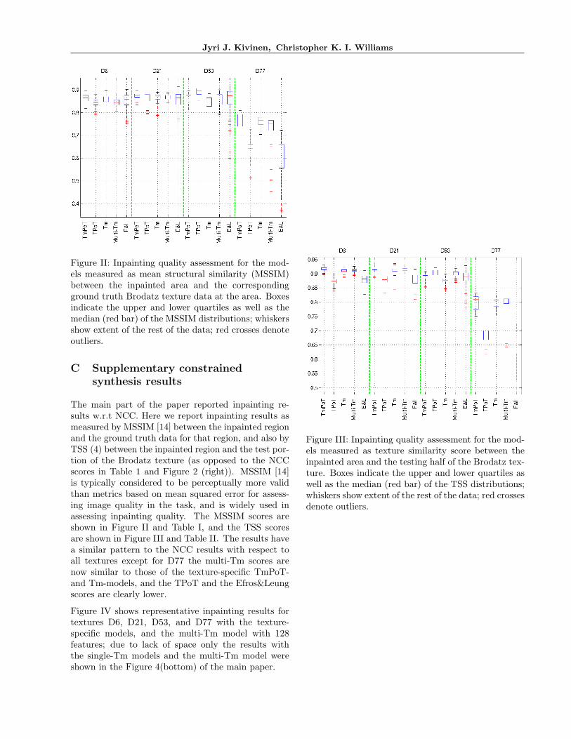
Figure II: Inpainting quality assessment for the mod-els measured as mean structural similarity (MSSIM)between the inpainted area and the correspondingground truth Brodatz texture data at the area. Boxesindicate the upper and lower quartiles as well as themedian (red bar) of the MSSIM distributions; whiskersshow extent of the rest of the data; red crosses denoteoutliers.
C Supplementary constrainedsynthesis results
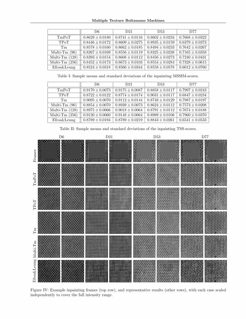
The main part of the paper reported inpainting re-sults w.r.t NCC. Here we report inpainting results asmeasured by MSSIM [14] between the inpainted regionand the ground truth data for that region, and also byTSS (4) between the inpainted region and the test por-tion of the Brodatz texture (as opposed to the NCCscores in Table 1 and Figure 2 (right)). MSSIM [14]is typically considered to be perceptually more validthan metrics based on mean squared error for assess-ing image quality in the task, and is widely used inassessing inpainting quality. The MSSIM scores areshown in Figure II and Table I, and the TSS scoresare shown in Figure III and Table II. The results havea similar pattern to the NCC results with respect toall textures except for D77 the multi-Tm scores arenow similar to those of the texture-specific TmPoT-and Tm-models, and the TPoT and the Efros&Leungscores are clearly lower.
Figure IV shows representative inpainting results fortextures D6, D21, D53, and D77 with the texture-specific models, and the multi-Tm model with 128features; due to lack of space only the results withthe single-Tm models and the multi-Tm model wereshown in the Figure 4(bottom) of the main paper.
Figure III: Inpainting quality assessment for the mod-els measured as texture similarity score between theinpainted area and the testing half of the Brodatz tex-ture. Boxes indicate the upper and lower quartiles aswell as the median (red bar) of the TSS distributions;whiskers show extent of the rest of the data; red crossesdenote outliers.
Multiple Texture Boltzmann Machines
D6 D21 D53 D77TmPoT 0.8629± 0.0180 0.8741± 0.0116 0.8602± 0.0234 0.7668± 0.0322TPoT 0.8446± 0.0172 0.8609± 0.0275 0.8935± 0.0159 0.6379± 0.0373Tm 0.8578± 0.0160 0.8662± 0.0185 0.8494± 0.0233 0.7642± 0.0267
Multi-Tm (96) 0.8267± 0.0169 0.8556± 0.0119 0.8325± 0.0238 0.7165± 0.0358Multi-Tm (128) 0.8393± 0.0154 0.8608± 0.0112 0.8456± 0.0273 0.7240± 0.0431Multi-Tm (256) 0.8452± 0.0173 0.8673± 0.0103 0.8554± 0.0284 0.7328± 0.0615
Efros&Leung 0.8524± 0.0318 0.8566± 0.0344 0.8558± 0.0578 0.6012± 0.0760
Table I: Sample means and standard deviations of the inpainting MSSIM-scores.
D6 D21 D53 D77TmPoT 0.9170± 0.0073 0.9175± 0.0087 0.8858± 0.0117 0.7997± 0.0243TPoT 0.8722± 0.0122 0.8774± 0.0174 0.9031± 0.0117 0.6847± 0.0234Tm 0.9095± 0.0070 0.9112± 0.0144 0.8748± 0.0129 0.7987± 0.0197
Multi-Tm (96) 0.8854± 0.0070 0.8939± 0.0073 0.8624± 0.0112 0.7573± 0.0208Multi-Tm (128) 0.8975± 0.0066 0.9018± 0.0064 0.8791± 0.0112 0.7674± 0.0188Multi-Tm (256) 0.9120± 0.0060 0.9148± 0.0064 0.8989± 0.0106 0.7960± 0.0370
Efros&Leung 0.8789± 0.0194 0.8789± 0.0219 0.8843± 0.0261 0.6541± 0.0533
Table II: Sample means and standard deviations of the inpainting TSS-scores.
D6 D21 D53 D77
Fram
esT
mP
oTT
PoT
Tm
Mul
ti-T
mE
fros
&L
eung
Figure IV: Example inpainting frames (top row), and representative results (other rows), with each case scaledindependently to cover the full intensity range.


![From Lattice Boltzmann Method to Lattice Boltzmann Flux … · From Lattice Boltzmann Method to Lattice Boltzmann Flux Solver Yan Wang 1, ... flows [8,13–15], compressible flows](https://static.fdocuments.us/doc/165x107/5cadf91b88c9938f4d8c0cd6/from-lattice-boltzmann-method-to-lattice-boltzmann-flux-from-lattice-boltzmann.jpg)