SUPPLEMENTARY INFORMATION

Impacts of Cattle, Hunting,

and Natural Gas Development

in a Rangeland Ecosystem

Cisneros-Pineda, Alfredo; Aadland, David; and Tschirhart, John

Department of Economics

University of Wyoming

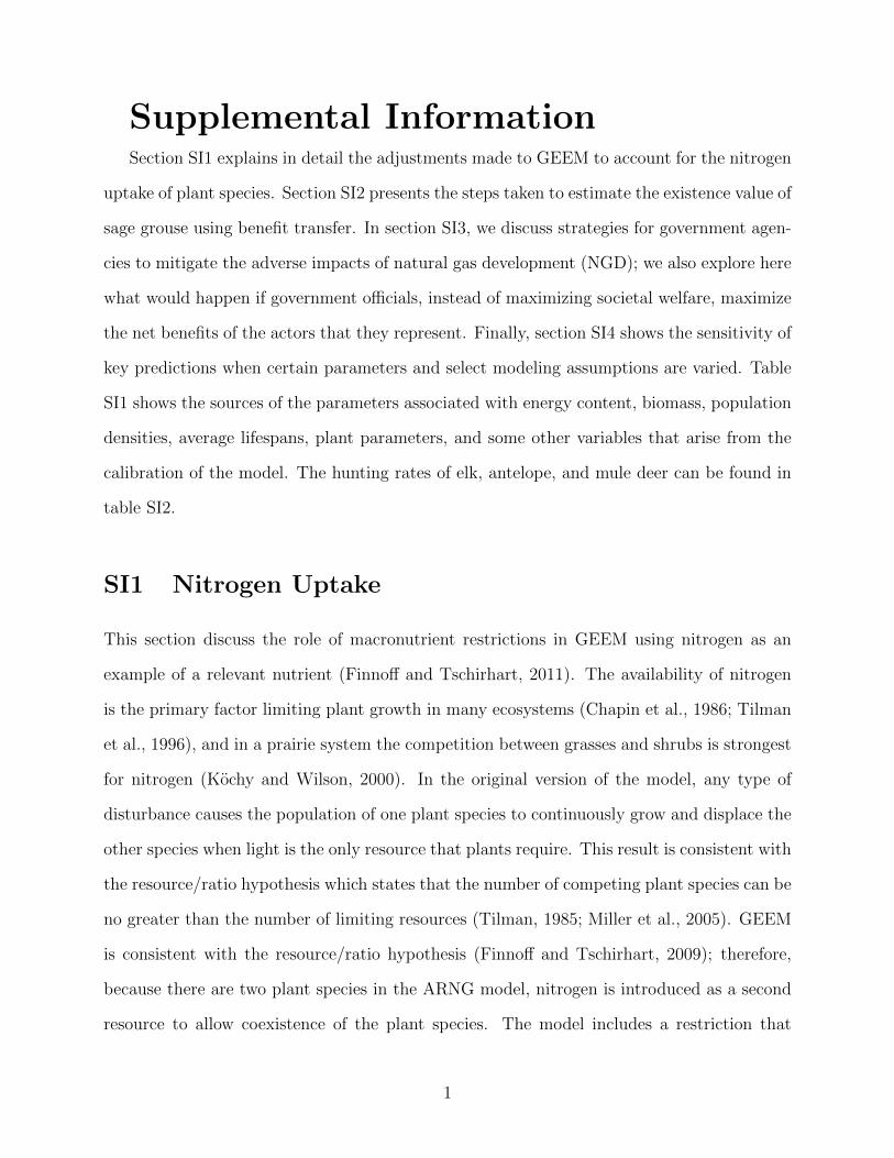
Supplemental InformationSection SI1 explains in detail the adjustments made to GEEM to account for the nitrogen

uptake of plant species. Section SI2 presents the steps taken to estimate the existence value of

sage grouse using benefit transfer. In section SI3, we discuss strategies for government agen-

cies to mitigate the adverse impacts of natural gas development (NGD); we also explore here

what would happen if government officials, instead of maximizing societal welfare, maximize

the net benefits of the actors that they represent. Finally, section SI4 shows the sensitivity of

key predictions when certain parameters and select modeling assumptions are varied. Table

SI1 shows the sources of the parameters associated with energy content, biomass, population

densities, average lifespans, plant parameters, and some other variables that arise from the

calibration of the model. The hunting rates of elk, antelope, and mule deer can be found in

table SI2.

SI1 Nitrogen Uptake

This section discuss the role of macronutrient restrictions in GEEM using nitrogen as an

example of a relevant nutrient (Finnoff and Tschirhart, 2011). The availability of nitrogen

is the primary factor limiting plant growth in many ecosystems (Chapin et al., 1986; Tilman

et al., 1996), and in a prairie system the competition between grasses and shrubs is strongest

for nitrogen (Kochy and Wilson, 2000). In the original version of the model, any type of

disturbance causes the population of one plant species to continuously grow and displace the

other species when light is the only resource that plants require. This result is consistent with

the resource/ratio hypothesis which states that the number of competing plant species can be

no greater than the number of limiting resources (Tilman, 1985; Miller et al., 2005). GEEM

is consistent with the resource/ratio hypothesis (Finnoff and Tschirhart, 2009); therefore,

because there are two plant species in the ARNG model, nitrogen is introduced as a second

resource to allow coexistence of the plant species. The model includes a restriction that

1

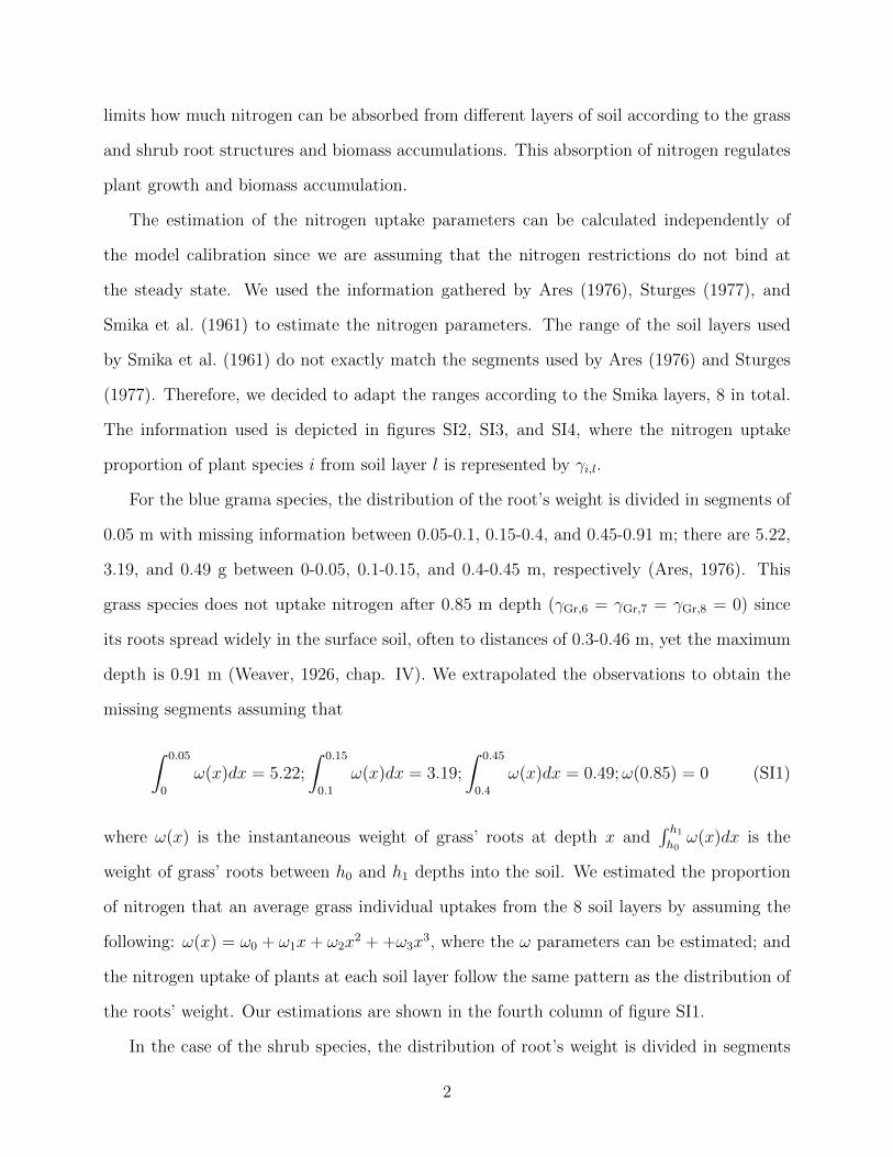
limits how much nitrogen can be absorbed from different layers of soil according to the grass

and shrub root structures and biomass accumulations. This absorption of nitrogen regulates

plant growth and biomass accumulation.

The estimation of the nitrogen uptake parameters can be calculated independently of

the model calibration since we are assuming that the nitrogen restrictions do not bind at

the steady state. We used the information gathered by Ares (1976), Sturges (1977), and

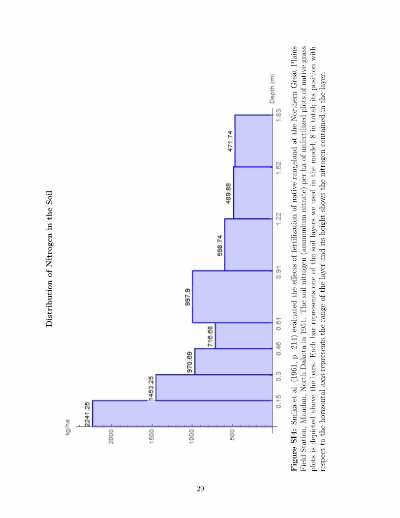
Smika et al. (1961) to estimate the nitrogen parameters. The range of the soil layers used

by Smika et al. (1961) do not exactly match the segments used by Ares (1976) and Sturges

(1977). Therefore, we decided to adapt the ranges according to the Smika layers, 8 in total.

The information used is depicted in figures SI2, SI3, and SI4, where the nitrogen uptake

proportion of plant species i from soil layer l is represented by γi,l.

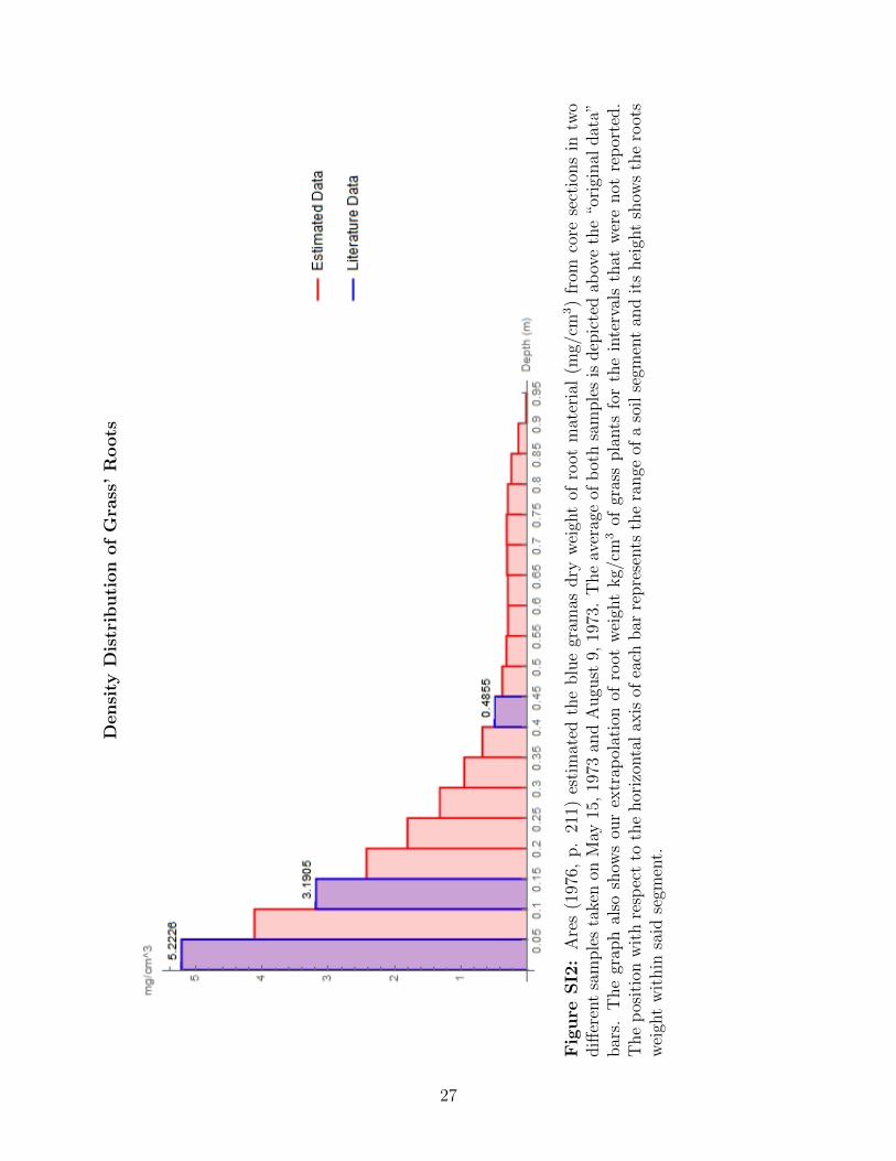
For the blue grama species, the distribution of the root’s weight is divided in segments of

0.05 m with missing information between 0.05-0.1, 0.15-0.4, and 0.45-0.91 m; there are 5.22,

3.19, and 0.49 g between 0-0.05, 0.1-0.15, and 0.4-0.45 m, respectively (Ares, 1976). This

grass species does not uptake nitrogen after 0.85 m depth (γGr,6 = γGr,7 = γGr,8 = 0) since

its roots spread widely in the surface soil, often to distances of 0.3-0.46 m, yet the maximum

depth is 0.91 m (Weaver, 1926, chap. IV). We extrapolated the observations to obtain the

missing segments assuming that

∫ 0.05

0

ω(x)dx = 5.22;

∫ 0.15

0.1

ω(x)dx = 3.19;

∫ 0.45

0.4

ω(x)dx = 0.49;ω(0.85) = 0 (SI1)

where ω(x) is the instantaneous weight of grass’ roots at depth x and∫ h1h0ω(x)dx is the

weight of grass’ roots between h0 and h1 depths into the soil. We estimated the proportion

of nitrogen that an average grass individual uptakes from the 8 soil layers by assuming the

following: ω(x) = ω0 + ω1x+ ω2x2 + +ω3x

3, where the ω parameters can be estimated; and

the nitrogen uptake of plants at each soil layer follow the same pattern as the distribution of

the roots’ weight. Our estimations are shown in the fourth column of figure SI1.

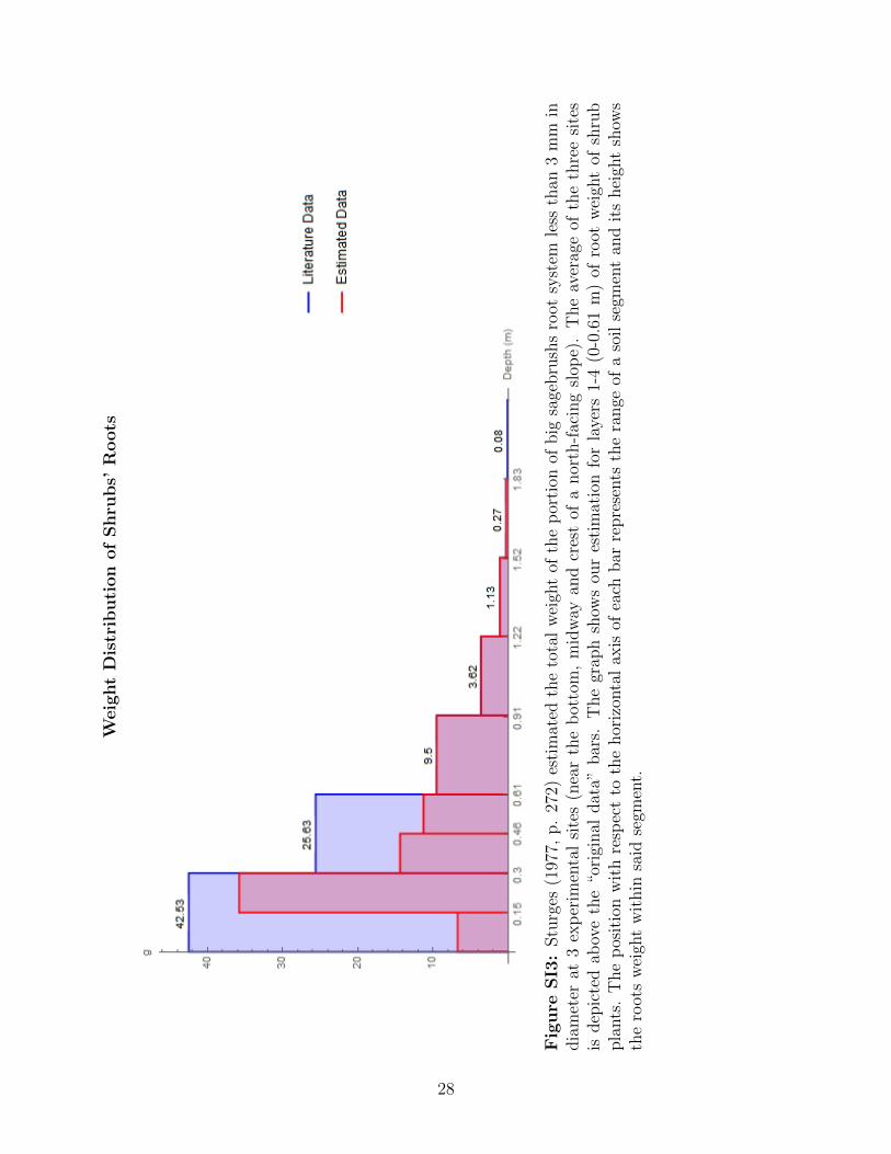
In the case of the shrub species, the distribution of root’s weight is divided in segments

2

of about 0.3 m (Sturges, 1977, p. 272). This distribution fits the Smika layers 5, 6, 7, and

8, but the rest of the layers do not match the segments used in Smika research. Since the

average total weight of shrub’s roots is 82.76 g (Sturges, 1977, p. 272) (and by assuming

that the nitrogen uptake follows the same pattern as the distribution of the roots’ weight),

then the uptake proportion is simply calculated by dividing the weight in each segment by

the total. Our estimations are shown in the last column of figure SI1. The uptake proportion

in layers 1-4 is still unknown because the Smika layers 1 and 2 are exactly contained in the

first Sturges segment and Smika layers 3 and 4 are exactly contained in the second Sturges

segment. Since there are 42.53 and 25.63 g in the first and second segments, we get that

γSh,1 + γSh,2 = 42.5382.76

= 51% and γSh,3 + γSh,4 = 25.6382.76

= 31%.

The nitrogen uptake proportions are necessary to model the balance between the nitrogen

that a plant loses and the nitrogen that the plant maintains internally. Plants use nitrogen

to produce biomass, and they continuously lose nitrogen for chemical and predatory reasons

(Berendse and Aerts, 1987). The nitrogen uptake of plant species i from layer l is

ηi,l = ϑinixiγi,l (SI2)

where ϑi is the minimum requirement of nitrogen for every kilogram of biomass (xi) that

the plant accumulates to satisfy the loss of nitrogen and production of biomass; and γi,l

is the uptake proportion that plant species i uptakes from the l-th soil layer. To estimate

the missing proportion nitrogen uptake of shrubs (γSh,i for i = 1, 2, 3, 4) and the minimum

requirements of nitrogen per kg (ϑGr,ϑSh), we solve for

3

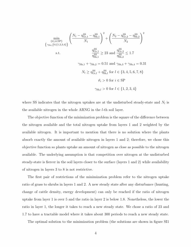
min{ϑi|i∈SP}

{γSh,l|l∈{1,2,3,4}}

(N1 − ηSSGr,1 − ηSSSh,1

N1

)2

+

(N2 − ηSSGr,2 − ηSSSh,2

N2

)2

s.t.ηSSGr,1

ηSSSh,1≥ 23 and

ηSSGr,2

ηSSSh,2≤ 1.7

γSh,1 + γSh,2 = 0.51 and γSh,3 + γSh,4 = 0.31

Nl ≥ ηSSGr,l + ηSSSh,l for l ∈ {3, 4, 5, 6, 7, 8}

ϑi > 0 for i ∈ SP

γSh,l > 0 for l ∈ {1, 2, 3, 4}

where SS indicates that the nitrogen uptakes are at the undisturbed steady-state and Nl is

the available nitrogen in the whole ARNG in the l-th soil layer.

The objective function of the minimization problem is the square of the difference between

the nitrogen available and the total nitrogen uptake from layers 1 and 2 weighted by the

available nitrogen. It is important to mention that there is no solution where the plants

absorb exactly the amount of available nitrogen in layers 1 and 2; therefore, we chose this

objective function so plants uptake an amount of nitrogen as close as possible to the nitrogen

available. The underlying assumption is that competition over nitrogen at the undisturbed

steady-state is fiercer in the soil layers closer to the surface (layers 1 and 2) while availability

of nitrogen in layers 3 to 8 is not restrictive.

The first pair of restrictions of the minimization problem refer to the nitrogen uptake

ratio of grass to shrubs in layers 1 and 2. A new steady state after any disturbance (hunting,

change of cattle density, energy development) can only be reached if the ratio of nitrogen

uptake from layer 1 is over 5 and the ratio in layer 2 is below 1.8. Nonetheless, the lower the

ratio in layer 1, the longer it takes to reach a new steady state. We chose a ratio of 23 and

1.7 to have a tractable model where it takes about 300 periods to reach a new steady state.

The optimal solution to the minimization problem (the solutions are shown in figure SI1

4

and table SI1) is such that there is an extra 9% of the nitrogen in layer 1 available for plants,

but plants uptake more nitrogen from layer 2 than the actual nitrogen available (8%). For

this minimization problem there is no solution where the uptake is lower than the nitrogen

available for both soil layers, therefore, we allowed for solutions where uptakes can be greater

than the nitrogen available as long as they are close enough.

The solution along with our estimations of nitrogen uptake of grass are consistent with

Sala et al. (2012); their experimental evidence of mineral nitrogen and absorption patterns

indicated that grasses showed a disproportionately large absorption from the uppermost layer,

a smaller value at 0.3 m, and practically no absorption after 0.6 m of depth; meanwhile, shrubs

showed no absorption in the shallow layers and most of the absorption occurred between 0.3

and 0.6 m of depth.

Since the growth of plants is already restricted at the undisturbed steady-state by the

limited amount of vertical space, we allowed for some flexibility by assuming that there is an

extra 1% of the nitrogen uptake of plants in layers 1 and 2 with respect to the undisturbed

steady-state such that

N∗l = 1.01(η∗Gr,l + η∗Sh,l

)for l ∈ {1, 2} (SI3)

where the asterisk indicates that the biomass accumulations and the populations are at the

undisturbed steady-state and that the optimal solution to the minimization problem is being

considered; N∗l is the adjusted available nitrogen in the ARNG in the l-th soil layer. In

the main text and the sensitivity analysis, we refer to these optimal parameters without

indicating the asterisk (N, ϑ, γ).

SI2 Benefit Transfer & Existence Value

The sage grouse is a high-profile species whose value must be considered among the ecosystem

services affected by NGD. No study that we know of has estimated the specific willingness

to pay (WTP) of households to secure the existence of a healthy population of sage grouse.

5

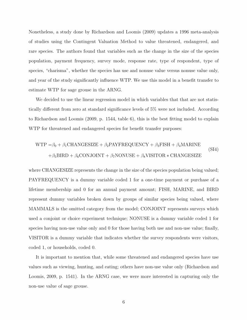
Nonetheless, a study done by Richardson and Loomis (2009) updates a 1996 meta-analysis

of studies using the Contingent Valuation Method to value threatened, endangered, and

rare species. The authors found that variables such as the change in the size of the species

population, payment frequency, survey mode, response rate, type of respondent, type of

species, “charisma”, whether the species has use and nonuse value versus nonuse value only,

and year of the study significantly influence WTP. We use this model in a benefit transfer to

estimate WTP for sage grouse in the ARNG.

We decided to use the linear regression model in which variables that that are not statis-

tically different from zero at standard significance levels of 5% were not included. According

to Richardson and Loomis (2009, p. 1544, table 6), this is the best fitting model to explain

WTP for threatened and endangered species for benefit transfer purposes:

WTP =β0 + β1CHANGESIZE + β2PAYFREQUENCY + β3FISH + β4MARINE

+β5BIRD + β6CONJOINT + β7NONUSE + β8VISITOR ∗ CHANGESIZE

(SI4)

where CHANGESIZE represents the change in the size of the species population being valued;

PAYFREQUENCY is a dummy variable coded 1 for a one-time payment or purchase of a

lifetime membership and 0 for an annual payment amount; FISH, MARINE, and BIRD

represent dummy variables broken down by groups of similar species being valued, where

MAMMALS is the omitted category from the model; CONJOINT represents surveys which

used a conjoint or choice experiment technique; NONUSE is a dummy variable coded 1 for

species having non-use value only and 0 for those having both use and non-use value; finally,

VISITOR is a dummy variable that indicates whether the survey respondents were visitors,

coded 1, or households, coded 0.

It is important to mention that, while some threatened and endangered species have use

values such as viewing, hunting, and eating; others have non-use value only (Richardson and

Loomis, 2009, p. 1541). In the ARNG case, we were more interested in capturing only the

non-use value of sage grouse.

6

To estimate the WTP per household of maintaining a stable population of sage grouse at

their undisturbed steady-state, we assumed a zero change in the population with an annual

payment amount for a bird species with non-use values. We also used the sample mean of

the CONJOINT variable (0.075), which results in an $11.38 WTP per household from the

following equation:

WTP = 11.38 =− 4.7 + 0.101(0) + 50.778(0) + 42.641(0) + 47.745(0) + 40.280(1)

+ 198.189(0.075)− 39.069(1) + 0.583(1)(0).

(SI5)

In the spirit of Loomis (2000), we measured the “relative benefit gradient” associated

with the existence value of the sage grouse species as a function of residential location. By

controlling for the quantity of public good being offered, and other variables reflecting indi-

vidual’s tastes and preferences, the author ran a regression to measure how WTP decreases

with respect to distance from the study area. Loomis (2000, p. 318) calculated the WTP

per household at 100 mile distance intervals from 100 miles to 2,500 miles.

Figure SI5 shows the assumed relationship between household WTP and distance. The

benefits received by local households (defined as those living within 100 miles of the ARNG

region) was set at 100%. The figure plots the percent of local household WTP for respondents

living at the other distances from the ARNG. As a reference, the percent of household benefits

drop faster than the Mexican Spotted Owl analyzed by Loomis (2000), implying zero benefits

per household beyond 1,800 miles from the Carbon County (e.g., households in Alaska receive

no benefit per household).

To replicate their methodology, we gathered the housing unit estimate per county as of

July 1, 2017 in the entire United States from the U.S. Census Bureau Population Division

(2018). Then, we proceeded to calculate the distance “as the crow flies” between the county

where the ARNG project is located, Carbon County, WY, and each of the 3,142 counties in

the U.S., by using the tool “How far is it between” (Free Map Tools, 2018).

Counties between 0 and 1,800 miles are assigned a percentage of WTP according to the

7

curve in figure SI5. For example, New York City has 886,408 housing units and is 1,704

miles away from Carbon, WY. According to the polynomial curve in figure SI5, 5.72% of

the WTP should be attributed to households residing in NYC with a total willingness to

pay of $576,591 to maintain the population of the sage grouse at the ARNG region. Adding

the distance-weighted WTP of all households across the U.S., we obtain a total value of

$264,180,054.

To translate this value into WTP per bird, we simply divid the total value by the popu-

lation of sage grouse in the ARNG region (2,732 birds), leading to a WTP/bird of $96,683.

It is important to mention that we are treating this as a lifetime value, not an annual flow.

SI3 Optimal Mitigation of Ecosystem Externalities &

Coordination Failure

In this section, we discuss possible mitigation strategies for the U.S. BLM and WGFD to

counteract some of the adverse impacts associated with NGD in the ARNG. We begin by

noting that the spatial impact of the gas wells and other anthropogenic features are not fully

incorporated into the model (Leu et al., 2008). For example, while we account for overlap in

the DAs (see figure 2 of the maint text), the simulations do not consider other spatial aspects

such as the impact of having eight separated clusters with different degrees of development

(see figure 3 in the main text). In future research, we intend to consider a spatial model that

respects well spacing, impacts on migration patterns of species, effects of roads, and possible

optimization of well location to maximize the ecosystem service benefits.

We also explore in this section what would happen if BLM and WGFD officials, instead

of maximizing societal welfare (as defined by the value of ecosystem services) after the in-

troduction of NGD, maximize the net benefits of the actors that they represent. If the BLM

represents the interests of ranchers and the WGFD represents the interests of hunters, then

a coordination failure could arise since cattle ranching and hunting impose ecosystem exter-

8

nalities on one another. The aforementioned ecosystem externalities are present even before

the introduction of NGD, but are likely to be exacerbated after the introduction of such a

large disturbance to the ecosystem.

Can government agencies coordinate to vary cattle stocking and hunting rates in the

ARNG region to increase the benefits that society derives from the rangeland ecosystem? The

question is complicated because of all the intra- and inter-species competition for resources

and the possible coordination difficulties across government agencies. In terms of grazing,

adding more cattle to the ecosystem may increase rancher profits because there are more

cattle to sell, but it also adds more competition for grass so cattle gain less weight that

reduces profit per head. Moreover, if the BLM reduces the cattle density, it may decrease

cattle profits, but there will be more grass available for other grass-eating species, such as elk.

In terms of WGFD management, changing the number of hunting licenses impacts rancher

profits. Issuing fewer elk (pronghorn and mule deer) licenses and increasing the herds imposes

a negative (positive) ecosystem externality on rancher profits. This follows because more elk

makes grass less abundant for cattle, and more pronghorn and mule deer makes grass more

abundant for cattle because it decreases shrub density, which in turn decreases the grasses’

loss of energy from shading and increase its biomass.

In a first attempt to address the coordination question, we perform a grid search to find the

optimal combination of cattle density and pronghorn hunting rates with GEEM, assuming,

for simplicity and tractability, that the elk and mule deer hunting rates remain fixed. The

pronghorn hunting rate and cattle density are selected in each simulation’s first period,

remain constant at those levels, and then the simulation runs until the ecosystem reaches

a steady state. The objective is to maximize the annual value of ecosystem services at the

post-development steady-state and reach the social optimum. We defined the optimization

problem with a constraint on the population of animal species. We performed a grid search

subject to the restriction that the population of no animal species can fall below 50% of the

original undisturbed steady-state. If the restriction binds, the simulation stops and the value

9

of ecosystem services is set to zero for the rest of the planning horizon. This is important

because otherwise it may be optimal to drive the populations of species to zero which violates

the U.S. Endangered Species Act and international treaties such as the 1940 Convention on

Nature Protection and Wildlife Preservation in the Western Hemisphere which states that

the Governments of the American Republics commit “to protect and preserve in their natural

habitat representatives of all species and genera of their native flora and fauna”.

The unconstrained optimization (not shown here) produces a extremely high hunting rate

that yields an immediate sharp drop in the pronghorn population, and has the potential of

irreversibly disrupting the ecosystem and driving the populations of grass and pronghorn to

zero. Also, with sufficient nitrogen another extreme scenario arises where grass completely

crowds out shrubs and the shrub-eaters (i.e., sage grouse, pronghorn and deer) also would

go extinct. Therefore, we consider an optimal management strategy where there is balanced

combination of pronghorn hunting and cattle density that can be maintained before the

restriction binds.

To keep the social planning problem tractable we restrict policy to only consider time-

invariant hunting and cattle stocking rates. This lack of flexibility imposed on the WGFD

and BLM may result in second-best outcomes. We hypothesize that the first-best strategy

might specify a higher cattle density in the short run while the grass is abundant, and then

slowly decrease cattle density, once hunting has reduced the population of herbivores and the

forage pressure on plants. We hope to consider time-varying strategies for future research.

Table SI3 shows the outcomes of a non-cooperative game between the BLM and the

WGFD at the post-development steady-state. The rows represent the possible pronghorn

hunting rates that the WGFD indirectly chooses by issuing hunting permits. The columns

represent the possible cattle densities that are implied by the public grazing permits issued

by the BLM. Inside each cell there are four values, all measured in millions of dollars: the top

left indicates the annual net benefits from hunting for elk, pronghorn, and mule deer if the

elk and mule deer hunting rates remain fixed according to the 2014 data (WGFD, 2014); the

10

top right indicates the annual profits of cattle ranching; the lower left is the annual existence

value of sage grouse; and the lower right is the annual value of ecosystem services. The

bold values are the best response of the WGFD to each action of the BLM and vice versa.

The shaded cells represent the Nash equilibrium (NE) whereby the strategies of both the

BLM and WGFD are best responses. The underlined value marks the social optimum that

considers all ecosystem services. Cells of only zeros represent combinations of hunting rates

and cattle densities that violate the population constraint.

As a point of clarification, consider the possibility where the WGFD issues enough

pronghorn hunting permits to allow a 22.61% annual reduction in the pronghorn popula-

tion and the BLM issues enough grazing permits to allow a seasonal cattle density of 0.0205

per ha. In this case, the benefits would be: $1.887 million for hunting net benefits, $2.665

million for cattle ranching profits, $9.4 for the existence value of sage grouse, and $13.95

million for annual value of all ecosystem services.

Some important remarks on table SI3: (1) when holding constant the hunting rate of

pronghorn (fixed on rows), increasing the cattle density puts extra foraging pressure on

grass which leads to a decrease of grass biomass (negatively affecting grass-eaters) and an

increase of shrub biomass (positively affecting shrub-eaters). This increases the net benefits

of pronghorn and mule deer hunting but decreases the benefits of elk hunting. The former

impact is greater than the latter impact and the total net benefits slowly increase with cattle

density. (2) When holding the cattle density constant (fixed on columns), increasing the

hunting rate has no effect on the profits of cattle grazing because cattle are already satiated

on grass. The hunting rate has an impact on cattle ranching profits only at higher cattle

densities.

The main message from table SI3 is that public policy without coordination between

the BLM and WGFD could lead to suboptimal outcomes. If WGFD and BLM officials

coordinate and respond immediately after the introduction of NGD, they can mitigate the

negative impacts of NGD on the ecosystem. Notice that the social optimum (hunting rate

11

of 0.2262 and cattle density of 0.032) of $15.7 million will not be chosen by the agencies

(because it is not a NE). In general, the most favorable outcomes (or NE) for the WGFD are

also the least favorable for the BLM and vice versa. There is no guarantee that the social

optimum will be selected if the two agencies do not coordinate.

SI4 Sensitivity Analysis

The application of GEEM in the estimation of impact of NGD relies on a number of modeling

assumptions and parameters. While some of the parameters were culled from ecological and

biological research papers, others had to be assumed within reasonable bounds. To account

for this inherent uncertainty, in this section we investigate how the predictions of the model

are altered when certain model assumptions or relevant parameters are changed.

First, we begin the sensitivity analysis in terms of one-time shocks on the populations

of the species in the sagebrush ecosystem. Here, the population shocks are not meant to

represent hunting or human gathering. The goal of introducing these type of shocks in the

model is to show the capacity of the system to self regulate and to isolate clearly two effects:

the short-run impacts versus the long-run impacts or the differences between steady states.

The population shocks were introduced into an ecosystem with no disturbances (i.e. no

cattle grazing, no hunting, and no NGD). Therefore, the cattle grazing profits and the hunting

benefits remain at zero and the value of ecosystem services depends only upon the populations

of sage grouse (existence value).

Table SI4 shows the discounted value of sage grouse existence value for different shock

scenarios. Each row represents a shock scenario, except for the first one that represents the

case where no shock is introduced to the ecosystem; the first column describes which species

are affected by the shocks and the second column indicates the magnitude of the shock. The

discounting considers all time periods between the introduction of the population shock (i.e.

the short run impacts on all the species and the associated ecosystem services), and the time

12

period when the ecosystem reaches a new steady state (long-run impacts).

Notice that big shocks do not necessarily translate into big changes in the value of ecosys-

tem services. For example, a 10% shock in the population of elk leads to a TDVES decrease

of about $0.694 million with respect to the baseline scenario ($264.18 million minus $263.486

million), while a 50% shock in the population of elk leads to a TDVES decrease of less than

$3.948 million ($264.18 million minus $260.232 million).

In the remainder sensitivity analysis, we are interested in analyzing how our estimate of

the negative impact of NGD changes with respect to the modeling assumptions and parameter

values. To do so, we estimated two discounted values: the discounted value of ecosystem

services already at the pre-NGD steady state (i.e. the value if NGD had never occurred),

and the discounted value after NGD is introduced to the ecosystem. Notice that the former

value considers annual flows that are constant, while the latter considers the adjustment and

responses of all the species.

The second sensitivity analysis varies the species that are affected by NGD. Table SI5

shows the discounted value of hunting benefits, cattle grazing profits, sage grouse existence

value, and the sum of all ecosystem services for different sensitivities to NGD for the key

species: mule deer, elk, and sage grouse. Each row represents a scenario; the first row

represents the undisturbed scenario. This scenario is not affected by NGD because the species

experience no stress when foraging in the DAs. The first column describes which species are

affected by NGD. The second, third, and fourth columns indicate the stress that the species

experience when foraging in the DA3, DA2, and DA1, respectively. The discounting in the

fifth, sixth, seventh, and eighth columns considers all periods between the introduction of

NGD (i.e. the short run impacts on all the species and the associated ecosystem services), and

the period when the ecosystem reaches a new steady state (long-run impacts). Finally, the

last column shows the estimated impact, which is calculated by subtracting the discounted

value of the introduction of NGD from the discounted value at the pre-NGD steady state.

The impact of NGD typically ranges between $0.124 and -$81.674 million.

13

The third sensitivity analysis considers changes in the parameters associated with the

root structure of the plant, which affects their capacity to uptake nitrogen from each soil

layer, and the nitrogen available in the soil layers. Table SI6 shows the discounted value

of hunting benefits, cattle grazing profits, sage grouse existence value, and the sum of all

services for scenarios associated to the nitrogen availability and uptake ratio of plants. Some

scenarios assumer higher or lower uptake ratios of nitrogen from the first and second soil

layers, others assume that there is more nitrogen available in the soil with respect to the

undisturbed scenario.

Each row represents a different nitrogen scenario and the first row is the baseline. Unlike

the sensitivity analysis described previously (species affected by NGD), changes in the pa-

rameters associated to nitrogen uptake and availability do affect the pre-NGD steady state.

Because cattle are assumed to gain 180 kg of weight when only that economic activity is

introduced into the ecosystem (see main text). The first, second, and third columns describe

what parameters change and the forth column indicates the type of steady state described.

The discounting for the ”Cattle Grazing + Hunting” scenario in the fifth, sixth, seventh, and

eighth columns considers a fixed annual flow of ecosystem services, while the discounting for

the ”Cattle Grazing + Hunting + NGD” scenario considers all periods between the introduc-

tion of NGD (short run impacts), and the period when the ecosystem reaches a new steady

state (long-run impacts). Finally, the last column shows the estimated negative impact of

introducing NGD.

The impact of NGD ranges between -$51.703 and -$60.416 million. In this sensitivity

analysis, the amount of extra nitrogen available for plants in the soil layers closer to the

surface is the most relevant feature. Although, the estimated impacts do not vary greatly.

As mentioned in the first section of this supplementary section, the nitrogen restrictions

mainly define how fast the ecosystem reaches a new steady state.

The fourth sensitivity analysis that we performed considers different WTP per household

to maintain the population of sage grouse at the undisturbed steady-state. Table SI7 shows

14

the discounted value of hunting benefits, cattle grazing profits, sage grouse existence value,

and the sum of all services for WTP varying between $1 and $14.

Each row of the table represents a different scenario. Unlike the previous sensitivity

analyses, the hunting benefits and the cattle grazing profits, remain unchanged because the

responses of all species are not affected and only the existence value is updated. The first

column describes the WTP/household assumed and the second column describes the scenario.

The discounting for the ”Cattle Grazing + Hunting” scenarios considers a fixed annual

flow of ecosystem services, while the discounting for the ”Cattle Grazing + Hunting + NGD”

scenarios considers the flow of ecosystem services in all periods. The last column shows the

estimated impact of NGD.

The impact of NGD ranges between -$17.019 and -$68.84 million and is fairly sensitive

to the assumed WTP per household. It is important to keep in mind that every single

household in the U.S. (except for Alaska and Hawaii households) are assumed to value the

sage grouse living in the ARNG region, depending on the distance to it. Since the existence

value considers such a large number of households, small changes in the WTP per household

have big impacts in terms of the aggregated value.

References

Alldredge, A., Lipscomb, J., and Whicker, F. (1974). Forage intake rates of mule deer

estimated with fallout cesium-137. The Journal of Wildlife Management, 38(3):152–156.

Anderson, J. and Shumar, M. (1986). Impacts of black-tailed jackrabbits at peak population

densities on sagebrush-steppe vegetation. Journal of Range Management, 39(2):152–156.

Anthony, R. and Smith, N. (1977). Ecological relationships between mule deer and white-

tailed deer in Southeastern Arizona. Ecological Monographs, 47(3):255–277.

15

Ares, J. (1976). Dynamics of the root system of blue grama. Journal of Range Management,

29(3):208–213.

Bakker, J. and Wilson, S. (2001). Competitive abilities of introduced and native grasses.

Plant Ecology, 157:117–125.

Berendse, F. and Aerts, R. (1987). Nitrogen-use-efficiency: A biologically meaningful defini-

tion? Functional Ecology, 1(3):293–296.

Biodiversity Conservation Alliance (2005). The special values of the Great Divide. National

Wildlife Federation.

Brody, S. and Procter, R. (1932). Relation between basal metabolism and mature body

weight in different species of mammals and birds. University of Missouri Agricultural

Experiment Station Research Bulletin, 166:89–101.

Brody, S., Procter, R., and Ashworth, U. (1934). Basal metabolism, endogenous nitrogen,

creatinine, and neutral sulphur excretions as functions of body weight. University of

Missouri Agricultural Experiment Station Research Bulletin1, 166:89–101.

Byers, J. (1997). American Pronghorn: Social Adaptations and Ghosts of Predators Past.

University of Chicago Press, Chicago, IL.

Chapin, F., Vitousek, P., and Van Cleve, K. (1986). The nature of nutrient limitation in

plant communities. The American Naturalist, 127(1):48–58.

Comerford, W., Kime, L., and Harper, J. (2013). Beef background production. Retrieved July

27, 2016, from http://extension.psu.edu/business/ag-alternatives/livestock/

beef-and-dairy-cattle/beef-background-production/extension publication

file.

Dahl, P., Judge, J., Gallo, J., and England, A. (1993). Vertical distribution of biomass and

moisture in a prairie grass canopy. College of Engineering, Technical Reports.

16

Davies, K. and Bates, J. (2010). Vegetation characteristics of mountain and Wyoming big

sagebrush plant communities in the Northern Great Basin. Rangeland Ecology and Man-

agement, 63(4):461–466.

Dietz, D. (1972). Nutritive value of shrubs. In Wildland Shrubs - Their Biology and Utiliza-

tion. U.S. Department of Agriculture Intermountain Forest and Range Experiment Starion

General Technical Report INT-1, Ogden, UT.

Egoscue, H., Bittmenn, J., and Petrovich, J. (1970). Some fecundity and longevity records

for captive small mammals. Journal of Mammalogy, 51(3):622–623.

Fagerstone, K., Lavoie, G., and Griffith, R. (1980). Black-tailed jackrabbit diet and density

on rangeland and near agricultural crops. Journal of Range Management, 33(3):229–233.

Fagerstone, K. and Ramey, C. (1996). Rodents and lagomorphs. The Society of Range

Management, Denver, CO.

Finnoff, D. and Tschirhart, J. (2009). Plant competition and exclusion with optimizing

individuals. Journal of Theoretical Biology, 261:227–237.

Finnoff, D. and Tschirhart, J. (2011). Inserting ecological detail into economic analysis:

Agricultural nutrient loading of an estuary fishery. Sustainability, 3:1688–1722.

Fraser, D. (2004). Factors influencing livestock behaviour and performance. Forest Practices

Branch, British Columbia Ministry of Forests, Rangeland Health Brochure 8, Victoria, BC.

Free Map Tools (2018). How far is it between. Retrieved August 8, 2018, from https://

www.freemaptools.com/how-far-is-it-between.htm.

Hansen, R. (1972). Estimation of herbage intake from jackrabbit feces. Journal of Range

Management, 25(6):468–471.

Hansen, R. and Reid, L. (1975). Diet overlap of deer, elk, and cattle in Southern Colorado.

Journal of Range Management, 28(1):43–47.

17

Hart, R. and Ashby, M. (1998). Grazing intensities, vegetation, and heifer gains: 55 years

on shortgrass. Journal of Range Management, 51(4):392–398.

Hitchcock, A. and Chase, A. (1950). Manual of the Grasses of the United States. U.S. Govt.

Print. Off., Washington, D.C., 2nd ed. edition.

Hudson, R. and Nietfeld, M. (1985). Effect of forage depletion on the feeding rate of wapiti.

Journal of Range Management, 38(1):80–82.

Jiang, Z. and Hudson, R. (1992). Estimating forage intake and energy expenditures of free-

ranging wapiti (cervus elaphus). Canadian Journal of Zoology, 70(4):675–679.

Johnson, M. (1979). Foods of primary consumers on cold desert shrub-steppe of Southcentral

Idaho. Journal of Range Management, 32(5):365–368.

Johnson, R. and Anderson, J. (1984). Diets of black-tailed jackrabbits in relation to popula-

tion density and vegetation. Journal of Range Management, 37(1):79–83.

Jurik, T. and Kleibenstein, H. (2000). Canopy architecture, light extinction and self-shading

of a prairie grass, Andropogon gerardii. American Midland Naturalist, 144(1):51–65.

Kelsey, R., Nelson, A., Smith, G., and Peiper, R. (1973). Nutritive value of hay from

nitrogen-fertilized blue gramma rangeland. Journal of Range Management, 26(4):292–294.

Kleiber, M. (1975). The fire of life: An introduction to animal energetics. Robert E. Krieger

Publishing Co., Huntington, NY, rev. edition.

Kochy, M. and Wilson, S. (2000). Competitive effects of shrubs and grasses in prairie. Oikos,

91:385–395.

Lambers, H., Chapin, F., and Pons, T. (2006). Plant Physiological Ecology. Springer, New

York, NY, 2nd edition.

18

Leu, M., Hanser, S., and Knick, S. (2008). The human footprint in the west: A large-scale

analysis of anthropogenic impacts. Ecological Applications, 18(5):1119–1139.

Loomis, J. (2000). Vertically summing public good demand curves: An empirical comparison

of economic versus political jurisdictions. Land Economics, 76(2):312–321.

Mackie, R., Kie, J., Pac, D., and Hamlin, K. (2003). Mule deer odocoileus hemionus. In

Feldhamer, G. A., Thompson, B. C., and Chapman, J. A., editors, Wild Mammals of North

America: Biology, Management, and Conservation, pages 889–905. The Johns Hopkins

University Press, Baltimore, MD.

Mackie, R., Pac, D., Hamlin, K., and Dusek, G. (1998). Ecology and management of mule

deer and white-tailed deer in Montana. Montana Department of Rish, Widlife and Parks.

Miller, T., Burns, J., Munguia, P., Walters, E., Kneitel, J., Richards, P., Mouquet, N., and

Buckley, H. (2005). A critical review of twenty years’ use of the resourceratio theory. The

American Naturalist, 165(4):439–448.

Ngugi, K., Powell, J., Hinds, F., and Olson, R. (1992). Range animal diet composition in

Southcentral Wyoming. Journal of Range Management, 45(6):542–545.

Olsen, F. and Hansen, R. (1977). Food relations of wild free-roaming horses to livestock and

big game, Red Desert, Wyoming. Journal of Range Management, 30(1):17–20.

Pac, D., Mackie, R., and Jorgensen, H. (1991). Mule deer population organization, behavior,

and dynamics in a Northern Rocky Mountain environment. Montana Department of Fish,

Wildlife and Parks, Final Report, Federal Aid in Wildlife Restoration Project W-120-R,

Montana.

Pyle, W. and Crawford, J. (1996). Availability of foods of sage grouse chicks following

prescribed fire in sagebrush- bitterbrush. Journal of Range Management, 49(4):320–324.

19

Reich, P., Ellsworth, D., and Walters, D. (1998). Leaf structure (specific leaf area) modulates

photosynthesis-nitrogen relations: Evidence from within and across species and functional

groups. Functional Ecology, 12(6):948–958.

Remington, T. and Braun, C. (1988). Carcass composition and energy reserves of sage grouse

during winter. The Condor, 90(1):15–19.

Richardson, L. and Loomis, J. (2009). The total economic value of threatened, endangered

and rare species: An updated meta-analysis. Ecological Economics, 68:1535–1548.

Sage Grouse initiative (2016). Conserve our Western roots. Retrieved June 17, 2016, from

http://www.sagegrouseinitiative.com/roots/.

Sala, O., Golluscio, R., Lauenroth, W., and Roset, P. (2012). Contrasting nutrient-capture

strategies in shrubs and grasses of a Patagonian arid ecosystem. Journal of Arid Environ-

ments, 82:130–135.

Savory, C. (1978). Food consumption of red grouse in relation to the age and productivity

of heather. The Journal of Animal Ecology, 47(1):269–282.

Severson, K. and May, M. (1967). Food preferences of antelope and domestic sheep in

Wyoming’s Red Desert. Journal of Range Management, 20(1):21–25.

Severson, K., May, M., and Hepworth, W. (1980). Food preferences, carrying capacities,

and forage competition between antelope and domestic sheep in Wyoming’s Red Desert.

University of Wyoming Agricultural Experiment Station Bulletin, SM 10.

Smika, D., Haas, H., Rogler, G., and Lorenz, R. (1961). Chemical properties and moisture

extraction in rangeland soils as influenced by nitrogen fertilization. Journal of Range

Management, 14(4):213–216.

Stewart, K., Bowyer, R., Dick, B., Johnson, B., and Kie, J. (2005). Density-dependent

20

effects on physical condition and reproduction in North American elk: An experimental

test. Oecologia, 143:85–93.

Stinson, D., Hays, D., and Schroeder, M. (2004). Washington State recovery plan for the

greater sage-grouse. Washington Department of Fish and Wildlife.

Sturges, D. (1977). Soil water withdrawal and root characteristics of big sagebrush. The

American Midland Naturalist, 98(2):257–274.

Tilman, D. (1985). The resource-ratio hypothesis of plant succession. The American Natu-

ralist, 125(6):827–852.

Tilman, D., Wedin, D., and Knops, J. (1996). Productivity and sustainability influenced by

biodiversity in grassland ecosystems. Nature, 379:718–720.

U.S. Census Bureau Population Division (2018). Annual estimates of housing units for the

United States, regions, Divisions, States, and Counties: April 1, 2010 to July 1, 2017.

Retrieved July 12, 2018, from https://factfinder.census.gov/faces/tableservices/

jsf/pages/productview.xhtml?src=bkmk.

Walker, B., Kinzig, A., and Langridge, J. (1999). Plant attribute diversity, resilience, and

ecosystem function: The nature and significance of dominant and minor species. Ecosys-

tems, 2(2):95–113.

Weaver, J. (1926). Root habits of native plants an how they indicate crop behavior. In

Weaver, J. E., editor, Root Development of Field Crops, chapter IV. McGraw-Hill Book

Company, New York, NY, 1st edition.

WGFD (2014). Annual reports of big and trophy game harvest and annual reports of small

and upland game harvest. Retrieved October 16, 2014, from https://wgfd.wyo.gov/

Hunting/Harvest-Reports/.

21

Whitaker, J. (1980). The Audubon Society Field Guide to North American Mammals. Alfred

A. Knopf, New York, NY.

Yoakum, J. (2004). Distribution and abundance. In O’Gara, B. W. and Yoakum, J. D.,

editors, Pronghorn Ecology and Management, pages 75–105. University Press of Colorado,

Boulder, CO.

Zablan, M. (1993). Evaluation of sage grouse banding program in North Park, Colorado. Ms,

Colorado State University.

Zachow, R. (1997). Elk (Cervus elaphus). South Dakota Deparment of Game, Fish and

Parks, Division of Wildlife, Pierre, SD.

22

Cali

bra

tion

Para

mete

rs

Par

amet

ers

and

Var

iab

les

Pla

nts

Her

biv

ores

Gra

ssS

hru

bE

lkC

attl

eJac

k-

rab

bit

Pro

ng-

hor

nM

ule

Dee

rS

age

Gro

use

Den

sity

(in

dh

a-1)

1152

001

8000

20.

0496

30.

0387

435

0.03

60.

097

0.02

58

Bio

mas

sac

cum

ula

tion

xi

orco

nsu

mp

tion

xi,j

(kg)

0.01

0169

0.05

7961

026

2011

1325

.54*

99.4

(Gr)

28.4

(Sh

)12

2091

363

9.81

425

15

Gro

ssen

ergy

conte

nte i

(kca

lkg-

1)

4200

16

5068

17

Exti

nct

ion

par

amet

erki

0.31

80.

419

Ave

rage

life

span

l i(y

ears

)52

042

21

1422

123

724

1025

1026

927

Pre

dat

ion

riskp i

0.02

84*

0.01

33*

Lea

far

eas i

(m2

kg-

1)

1028

7.12

9

Min

imu

mn

itro

gen

requ

irem

entϑi

3.20

6*2.

637*

Bas

alm

etab

olis

mβi

(kca

lye

ar-1

)37

96*

1322

7*15

8121

230 1

2505

5431

5438

8.23

233

5584

33

5689

6734

4211

035

Ave

rage

wei

ghtwi

(kg)

0.02

1936

0.12

4637

315.

538

2733

93.

240

46.4

41

123.

842

1.54

3

Res

pir

atio

np

aram

eterr i

4364

6181

*46

7758

6*0.

4607

*2.

1301

3*8.

0533

*15

.365

2*2.

7799

*13

4.75

*

Par

amet

erof

the

wil

lin

gnes

sto

sup

plyg k,i

0.01

119*

0.00

73*

0.02

6*(G

r)0.

044*

(Sh

)0.

0032

6*0.

0299

*0.

0003

2*

Sh

adin

gen

ergy

loss

SE

Li

oren

ergy

exp

end

itu

rep

ricee k,i

(kca

lkg-

1)

5442

8*67

768*

2992

.51*

1374

.31*

3277

*(G

r)44

31*(S

h)

1841

.3*

3286

.64*

1564

.48*

Table

SI1

:T

he

aste

risk

(*)

indic

ates

that

the

par

amet

er/v

aria

ble

ises

tim

ated

by

assu

min

gth

atth

eec

osyst

emis

atst

eady

stat

e.T

he

stea

dy

stat

eth

atar

ises

afte

rca

ttle

are

intr

oduce

dto

the

ecos

yst

emis

use

dto

calibra

teth

eir

par

amet

ers.

The

undis

turb

edst

eady-s

tate

isuse

dfo

ral

lot

her

spec

ies.

23

1From studies of Wyoming big sagebrush and mountain big sagebrush (Artemisia tridentata) communi-ties in south east Oregon that contain the native grasses common to Wyoming: Idaho fescue (Festuca ida-hoensis), prairie junegrass (Koeleria macrantha), bluebunch wheatgrass (Pseudoroegneria spicata), Thurbersneedlegrass (Achnatherum thurberianum), needle and thread (Hesperostipa comata), squirreltail (Elymuselymoides), and Sandberg bluegrass (Poa secunda). Davies and Bates (2010, p. 464) report grass densitiesof both communities and we use an average of 11.52 individual (ind) plants m-2 or 115200 ind ha-1.

2See footnote 1. An average of Wyoming big sagebrush density (1.1 ind m-2) and mountain big sagebrush(0.5 ind m-2) was used to obtain 8,000 ind ha-2 (Davies and Bates, 2010, p. 464).

3Stewart et al. (2005) state a high and low population density of 4.51 elk km-2 - 5.41 elk km-2. The meanvalue of approximately 4.96 elk km-2 is used here (0.0496 elk ha-1).

4According to the EIS, there are 31 relevant BLM grazing allotments in the ARNG and the surroundingarea, which allows for a total of 39,695 animal unit months (AUMs). Only a portion of this allotment isin the ARNG. To estimate the cattle density, we assume that the number of AUMs inside the ARNG isproportional to the acreage in the ARNG. This results in 21,135 AUMs inside the ARNG. Assuming eachanimal is allowed to graze for 5 months implies a total of 4,227 individual steers and heifers grazing insidethe ARNG. Since there are 109,297 ha in the ARNG, the estimated cattle grazing density is 0.0387.

5Studies have reported jackrabbit densities between 0.02 ha-1 and 35 ha-1 (Anderson and Shumar, 1986;Fagerstone et al., 1980; Fagerstone and Ramey, 1996), where the highest density estimates are usually ob-served around agricultural lands. The density estimate used is 3 ha-1.

6Yoakum (2004) reports a pronghorn density for Wyoming of 3.0 ind km-2, or 0.03 ha-1.7BLM lands hold over 323,748.5 ha of crucial range for 85,000 mule deer within the great divide resource

management area (Biodiversity Conservation Alliance, 2005). This translates to 0.2625 mule deer ha-1.8A study of the Hart Mountain National Pronghorn Refuge in Lake County, Oregon revealed a sage grouse

density in the 1980s of 2.5 birds km-2 which is converted to 0.025 grouse ha-1 (Pyle and Crawford, 1996).9Using data from footnote 1, the average biomass production of grasses over both communities was 300

kg ha-1 (Davies and Bates, 2010, p. 464). We assumed this was grazed with a moderate intensity as definedby cattle grazing and note that ungrazed blue gamma has 667

397 = 1.68 more standing biomass than grazedblue gamma (Hart and Ashby, 1998, p. 394). Applying this yields 504 kg ha-1. Also, Hart and Ashby (1998)report blue gamma biomass of 667 kg ha-1 which is averaged with data from Davies and Bates (2010) toobtain 585.5 kg ha-1. We convert to wet weight with a ratio of wet weight to dry weight ratio of 2 (Dahlet al., 1993) to obtain 1,171 kg ha-1. Finally, dividing by the number of plants yields 0.01016 kg ind-1.

10Severson and May (1967) report annual forage production for Wyoming big sagebrush to be 206.85 lbDW acre-1. This is converted to (206.85 lb DW acre-1) (2 WW DW-1) (0.453592 kg lb-1) (2.471 acre ha-1)(ha (8000 ind)-1) = 0.05796 kg WW ind-1.

11Estimates of daily forage intake for elk range from 7 kg days-1 (Fraser, 2004; Jiang and Hudson, 1992) to9.5 kg days-1 (Hudson and Nietfeld, 1985). Using the average, annual forage intake is 3011 kg. Ngugi et al.(1992) study diet composition of grazing and browsing animals in South central Wyoming and report thatelk diet consisted 84% to 90% of grass. We used the average of 87% to scale elk demand for grass down to2620 kg years-1.

12Hansen (1972) estimates an intake rate of 0.389 kg days-1 for jackrabbits. This is extrapolated to anintake of 141.985 kg years-1. For shrub-steppe and mixed shrub-grass communities, diet composition of 70%grass and 20% shrub is used (Johnson, 1979; Johnson and Anderson, 1984). This is translated to an annualintake of 99.39 kg (of grasses) and 28.40 kg (of shrubs).

13Severson et al. (1980) report pronghorn daily forage intake rate to be 0.8 kg ind-1, which is converted to292 kg ind-1 years-1. Annual pronghorn diet consisted from 65% to 78% sagebrush in South central Wyomingand in the Red Desert (Olsen and Hansen, 1977; Severson et al., 1980). The average is used to scale downannual forage requirement to 209 kg.

14Alldredge et al. (1974) report mean forage intake rate of 0.998 kg (45.36 kg)-1 day-1 for Colorado mule

24

deer. Using the weight, 123.8 kg, total intake is calculated: 994.2 kg years-1. See footnote 38. Shrubs havebeen documented to comprise between 46% and 82.7% of mule deer diets in various studies (Anthony andSmith, 1977; Hansen and Reid, 1975). The mean value of 64.35% is used to scale the forage requirementdown to 639.8 kg year-1.

15 Savory (1978) studies food intake of red grouse in Scotland and reports that annual intake vary from 18kg to 25 kg (both in terms of dry weight). The higher estimate is taken to be a reasonable approximation ofthe food intake of sage grouse.

16From Kelsey et al. (1973, p. 293).17Dietz (1972) reports a gross energy content of 5.068 kcal g-1 for sagebrush from South Dakota. This is

converted to 5068 kcal kg-1.18The extinction coefficient is low for vertically inclined leaves (for example, 0.3-0.5 for grasses), but higher

for a more horizontal leaf arrangement (Lambers et al., 2006, p. 26).19See footnote 18. Light extinction for shrub formations is higher than for grasses. We use 0.4.20Perennials are assumed to have 5 years average longevity (Walker et al., 1999, p. 102).21In a Wyoming big sagebrush community in Wyoming the plants ranged from 26 to 57 years of age.

Average age reported of 42 years is used (Sturges, 1977).22The average lifespan for an elk is 14 to 16 years for males and 15 to 17 years for females (Zachow, 1997).

The lower value for males of 14 years is used.23Ranchers employ a stocker operation where they acquire young adult steers or heifers and graze them

for one season in a year before they are sent to market.24Egoscue et al. (1970) report that a captive black-tailed jackrabbit lived for 6 years and 9 months. In

calibration, 7 years is used as lifespan in the wild.25Pronghorns have an estimated lifespan of 5 to 15 years (Byers, 1997); we used the average of 10 years.26Maximum age for female mule deer range from 12 to 14 years, while for males it is 8 years (Pac et al.,

1991; Mackie et al., 1998, 2003). A life span of 10 years is used.27Greater sage grouse can survive at least 9 years in the wild (Zablan, 1993; Stinson et al., 2004).28Approximately the middle of the range for the inverse of g m-2 (Jurik and Kleibenstein, 2000, p. 58).29Reich et al. (1998) report that mean specific leaf area for evergreen shrubs is 71 cm2 g-1, or 7.1 m2 kg-1.30Brody et al. (1934) obtained M = 70.5ω0.734 as the power function relationship between daily metabolic

rate in kcal per day (M) and body weight in kg (ω) for mammals. Using a weight of 315.5 kg (footnote 38),total metabolic energy requirement is about 1,756,902 kcal year-1. Because 90% of elks diet is accounted forin the food web, the basal metabolism requirement is scaled down to 1,581,212 kcal year-1.

31For mammals, resting metabolic rate in kcal days-1 (M) is related to body weight (ω) in kg by theformula M = 67.61ω0.7565% (Kleiber, 1975). Weights are given in footnote 39. Extrapolating to a 6 monthseason for both weights yields 857,063-1,532,784 kcal season-1. The value used is 1,250,554 kcal season-1.

32Using the power function relationship and a jackrabbit weight of 3.2 kg (Fagerstone and Ramey, 1996),total metabolic energy requirement is 6,0431.32 kcal years-1. See footnote 30. This is scaled down to 54388.19kcal years-1 because only 90% of a jackrabbits diet is accounted for in the food web.

33Using a weight of 315.5 kg in the power function, total metabolic energy requirement is about 430,235kcal years-1. See footnotes 30 and 38. Because 78% of pronghorns diet is accounted, the basal metabolismrequirement is scaled down to 335,584 kcal years-1.

34Using the power function and the average mule deer weight 123.8 kg, the metabolic energy requirementis about 884,176 kcal years-1. See footnotes 30 and 38. Because 64.35% of a deers diet is accounted for inthe food web, the basal metabolism requirement is scaled down to 568,967 kcal years-1.

35Brody and Procter (1932) obtained M = 89ω0.64 as the power function relationship between dailymetabolic rate in kcal day-1 (M) and body weight in kg (ω) for wild birds. Using the weight of an adultfemale sage grouse of 1.5 kg (Remington and Braun, 1988), total metabolic energy requirement of 42,109.62kcal years-1 is calculated.

36If the biomass accumulation represents only the 46.5% of the total weight, the other 53.5% of comes from

25

Estimated Nitrogen Uptake of Grass and Shrubs

Figure SI1: The diagram depicts the root structure of blue grama (Bouteloua gracilis)(Weaver, 1926) and a drawing of the plant (Hitchcock and Chase, 1950). The diagram alsodepicts the root structure of the big sage brush (Artemisia tridentata) (Sage Grouse initiative,2016). The total nitrogen available in each soil layer comes from Smika et al. (1961). See theappendix for further details.

the weight of the roots (Bakker and Wilson, 2001).37See footnote 36.38 Weight is an average of the ranges of male and female weights from Whitaker (1980).39Weights of stocked cattle vary. We use typical weights of 273 kg per stocked feeder calf and 589 kg

market weight at the end of the stocking season (Comerford et al., 2013).40Jackrabbit weight is taken from Fagerstone and Ramey (1996).41See footnote 38.42See footnote 38.43Remington and Braun (1988).

26

Densi

tyD

istr

ibuti

on

of

Gra

ss’

Roots

Fig

ure

SI2

:A

res

(197

6,p.

211)

esti

mat

edth

eblu

egr

amas

dry

wei

ght

ofro

otm

ater

ial

(mg/

cm3)

from

core

sect

ions

intw

odiff

eren

tsa

mple

sta

ken

onM

ay15

,19

73an

dA

ugu

st9,

1973

.T

he

aver

age

ofb

oth

sam

ple

sis

dep

icte

dab

ove

the

“ori

ginal

dat

a”bar

s.T

he

grap

hal

sosh

ows

our

extr

apol

atio

nof

root

wei

ght

kg/

cm3

ofgr

ass

pla

nts

for

the

inte

rval

sth

atw

ere

not

rep

orte

d.

The

pos

itio

nw

ith

resp

ect

toth

ehor

izon

tal

axis

ofea

chbar

repre

sents

the

range

ofa

soil

segm

ent

and

its

hei

ght

show

sth

ero

ots

wei

ght

wit

hin

said

segm

ent.

27

Weig

ht

Dis

trib

uti

on

of

Shru

bs’

Roots

Fig

ure

SI3

:Stu

rges

(197

7,p.

272)

esti

mat

edth

eto

tal

wei

ght

ofth

ep

orti

onof

big

sage

bru

shs

root

syst

emle

ssth

an3

mm

india

met

erat

3ex

per

imen

tal

site

s(n

ear

the

bot

tom

,m

idw

ayan

dcr

est

ofa

nor

th-f

acin

gsl

ope)

.T

he

aver

age

ofth

eth

ree

site

sis

dep

icte

dab

ove

the

“ori

ginal

dat

a”bar

s.T

he

grap

hsh

ows

our

esti

mat

ion

for

laye

rs1-

4(0

-0.6

1m

)of

root

wei

ght

ofsh

rub

pla

nts

.T

he

pos

itio

nw

ith

resp

ect

toth

ehor

izon

tal

axis

ofea

chbar

repre

sents

the

range

ofa

soil

segm

ent

and

its

hei

ght

show

sth

ero

ots

wei

ght

wit

hin

said

segm

ent.

28

Dis

trib

uti

on

of

Nit

rogen

inth

eSoil

Fig

ure

SI4

:Sm

ika

etal

.(1

961,

p.

214)

eval

uat

edth

eeff

ects

offe

rtiliz

atio

nof

nat

ive

range

land

atth

eN

orth

ern

Gre

atP

lain

sF

ield

Sta

tion

,M

andan

,N

orth

Dak

ota

in19

51.

The

soil

nit

roge

n(a

mm

oniu

mnit

rate

)p

erha

ofunfe

rtiliz

edplo

tsof

nat

ive

gras

splo

tsis

dep

icte

dab

ove

the

bar

s.E

ach

bar

repre

sents

one

ofth

eso

illa

yers

we

use

din

the

model

,8

into

tal;

its

pos

itio

nw

ith

resp

ect

toth

ehor

izon

tal

axis

repre

sents

the

range

ofth

ela

yer

and

its

hei

ght

show

sth

enit

roge

nco

nta

ined

inth

ela

yer.

29

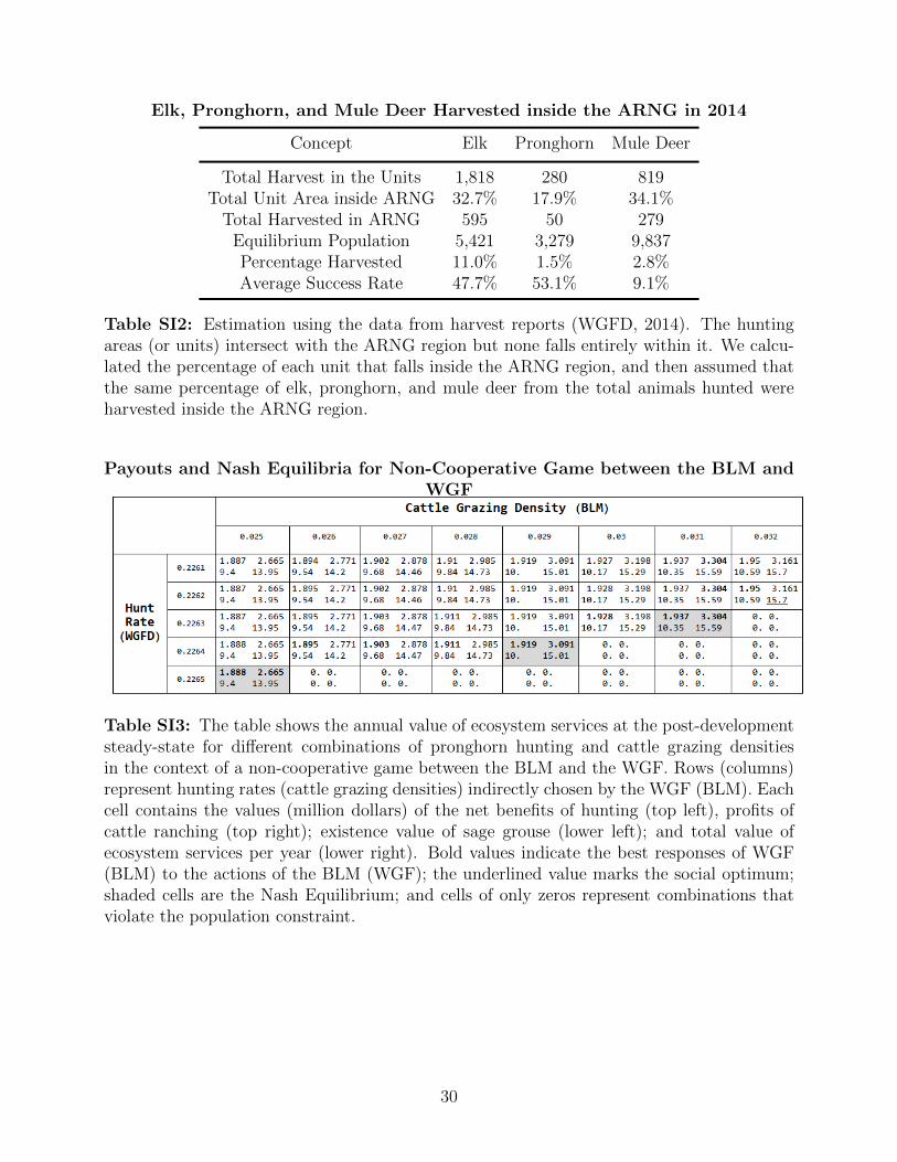
Elk, Pronghorn, and Mule Deer Harvested inside the ARNG in 2014

Concept Elk Pronghorn Mule Deer

Total Harvest in the Units 1,818 280 819Total Unit Area inside ARNG 32.7% 17.9% 34.1%

Total Harvested in ARNG 595 50 279Equilibrium Population 5,421 3,279 9,837Percentage Harvested 11.0% 1.5% 2.8%Average Success Rate 47.7% 53.1% 9.1%

Table SI2: Estimation using the data from harvest reports (WGFD, 2014). The huntingareas (or units) intersect with the ARNG region but none falls entirely within it. We calcu-lated the percentage of each unit that falls inside the ARNG region, and then assumed thatthe same percentage of elk, pronghorn, and mule deer from the total animals hunted wereharvested inside the ARNG region.

Payouts and Nash Equilibria for Non-Cooperative Game between the BLM andWGF

Table SI3: The table shows the annual value of ecosystem services at the post-developmentsteady-state for different combinations of pronghorn hunting and cattle grazing densitiesin the context of a non-cooperative game between the BLM and the WGF. Rows (columns)represent hunting rates (cattle grazing densities) indirectly chosen by the WGF (BLM). Eachcell contains the values (million dollars) of the net benefits of hunting (top left), profits ofcattle ranching (top right); existence value of sage grouse (lower left); and total value ofecosystem services per year (lower right). Bold values indicate the best responses of WGF(BLM) to the actions of the BLM (WGF); the underlined value marks the social optimum;shaded cells are the Nash Equilibrium; and cells of only zeros represent combinations thatviolate the population constraint.

30

Per

house

hold

benefit

gra

die

nts

for

sage

gro

use

exis

tence

valu

e:

Perc

ent

of

loca

lW

TP

as

afu

nct

ion

of

dis

tan

cefr

om

habit

at

Fig

ure

SI5

:In

the

spir

itof

Loom

is(2

000,

p.

318)

,w

eas

sum

edth

atth

eW

TP

ofhou

sehol

ds

ofm

ainta

inin

ga

stab

lep

opula

tion

ofsa

gegr

ouse

dec

reas

esw

ith

dis

tance

from

hab

itat

.T

he

hor

izon

tal

axis

show

the

dis

tance

inm

iles

toth

eA

RN

Gre

gion

and

the

vert

ical

axis

show

sw

hat

per

centa

geof

the

loca

lb

enefi

tsin

the

Car

bon

Cou

nty

are

per

ceiv

edin

counti

esfu

rther

away

.

31

Sensi

tivit

yA

naly

sis:

One-T

ime

Shock

son

Popula

tions

Table

SI4

:T

he

table

show

sth

edis

counte

dva

lue

ofca

ttle

ranch

ing

pro

fits

,ex

iste

nce

valu

eof

sage

grou

se,

and

tota

lse

rvic

esfo

rdiff

eren

tp

opula

tion

shock

scen

ario

s.T

he

ligh

t-sh

aded

cells

show

the

min

imum

valu

ein

each

colu

mn,

while

the

dar

k-s

had

edce

lls

show

the

max

imum

valu

e.

32

Sensi

tivit

yA

naly

sis:

Sets

of

Sp

eci

es

Aff

ect

ed

by

NG

D

Table

SI5

:T

he

table

show

sth

edis

counte

dva

lue

ofhunti

ng

ben

efits

,ca

ttle

ranch

ing

pro

fits

,ex

iste

nce

valu

eof

sage

grou

se,

and

the

sum

ofal

lse

rvic

esfo

rdiff

eren

tco

mbin

atio

ns

ofsp

ecie

saff

ecte

dby

NG

D.

The

ligh

t-sh

aded

cells

show

the

min

imum

valu

ein

each

colu

mn,

while

the

dar

k-s

had

edce

lls

show

the

max

imum

valu

e.

33

Sensi

tivit

yA

naly

sis:

Nit

rogen

Avail

abil

ity

and

Upta

ke

Capaci

ty

Table

SI6

:T

he

table

show

sth

edis

counte

dva

lue

ofhunti

ng

ben

efits

,ca

ttle

ranch

ing

pro

fits

,ex

iste

nce

valu

eof

sage

grou

se,

and

the

sum

ofal

lse

rvic

esfo

rdiff

eren

tnit

roge

nupta

kera

tios

inth

eso

illa

yers

and

nit

roge

nav

aila

bilit

y.T

he

ligh

t-sh

aded

cells

show

the

min

imum

valu

ein

each

colu

mn,

while

the

dar

k-s

had

edce

lls

show

the

max

imum

valu

e.

34

Sensi

tivit

yA

naly

sis:

Sage

Gro

use

WT

P/H

ouse

hold

Table

SI7

:T

he

table

show

sth

edis

counte

dva

lue

ofhunti

ng

ben

efits

,ca

ttle

ranch

ing

pro

fits

,ex

iste

nce

valu

eof

sage

grou

se,

and

the

sum

ofal

lse

rvic

esfo

rdiff

eren

tW

TP

/hou

sehol

dto

mai

nta

inth

ep

opula

tion

ofsa

gegr

ouse

stab

leat

the

undis

turb

edst

eady-s

tate

.T

he

ligh

t-sh

aded

cells

show

the

hig

hes

tim

pac

t,w

hile

the

dar

k-s

had

edce

lls

show

the

low

est

impac

t.

35