Supplementary Information Graphene wrinkling induced … · S1.7. Spatial distribution of the...
12
Supplementary Information Graphene wrinkling induced by monodisperse nanoparticles: facile control and quantification Jana Vejpravova 1 *, Barbara Pacakova 1 , Jan Endres 2 , Alice Mantlikova 1 , Tim Verhagen 1 , Vaclav Vales 3 , Otakar Frank 3 and Martin Kalbac 3 ** 1 Institute of Physics AS CR, v.v.i., Department of Magnetic Nanosystems, Na Slovance 2, 18221 Prague 2, Czech Republic 2 Charles Univeristy in Prague, Faculty of Mathematics and Physics, Department of Condensed Matter Physics, Ke Karlovu 5, 12116 Prague 2, Czech Republic 3 JH Institute of Physical Chemistry AS CR,v.v.i., Dolejskova 3, 18200 Prague 8, Czech Republic *[email protected], **[email protected]
Transcript of Supplementary Information Graphene wrinkling induced … · S1.7. Spatial distribution of the...

Supplementary Information
Graphene wrinkling induced by monodisperse nanoparticles: facile control and
quantification
Jana Vejpravova1*, Barbara Pacakova
1, Jan Endres
2, Alice Mantlikova
1, Tim Verhagen
1,
Vaclav Vales3, Otakar Frank
3 and Martin Kalbac
3**
1Institute of Physics AS CR, v.v.i., Department of Magnetic Nanosystems, Na Slovance 2,
18221 Prague 2, Czech Republic
2Charles Univeristy in Prague, Faculty of Mathematics and Physics, Department of
Condensed Matter Physics, Ke Karlovu 5, 12116 Prague 2, Czech Republic
3JH Institute of Physical Chemistry AS CR,v.v.i., Dolejskova 3, 18200 Prague 8, Czech
Republic
S.1. Additional results of Raman mapping
S1.1. Typical Raman spectra of the GNP1-6 samples in the D-mode region together of the fit by a
single pseudo-Voigt function.
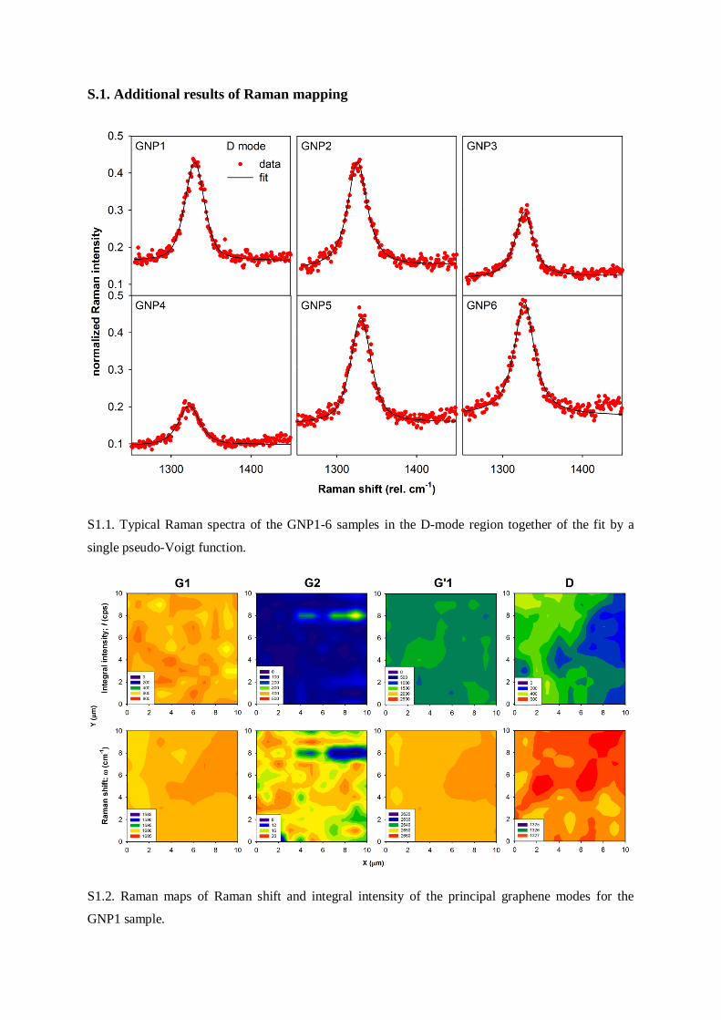
S1.2. Raman maps of Raman shift and integral intensity of the principal graphene modes for the
GNP1 sample.

S1.3. Raman maps of Raman shift and integral intensity of the principal graphene modes for the
GNP2 sample.
S1.4. Raman maps of Raman shift and integral intensity of the principal graphene modes for the
GNP3 sample.

S1.5. Raman maps of Raman shift and integral intensity of the principal graphene modes for the
GNP4 sample.
S1.6. Raman maps of Raman shift and integral intensity of the principal graphene modes for the
GNP6 sample.

S1.7. Spatial distribution of the relative intensity of the G2 with respect to the G1 mode for GNP1 –
GNP6 samples.
Table S1.1. Basic parameters obtained from analysis of the fine structure of the G and G’ mode:
FWHM – full width at half maxima and - fraction of the Lorentzian component. For the GNP3, the
best match of the G‘ was achieved for a single pseudo-Voigt peak with larger FWHM, therefore the
G’2 is just estimation from the less significant fit.
Sample FWHM G1
(cm-1
)
FWHM G2
(cm-1
)
G1
FWHM G’1
(cm-1
)
G’1 G’2
GNP1 14.8±0.8 15.0±0.2 0.69±0.11 39.5±1.5 0.60±0.04 0.57±0.32
GNP2 14.8±0.6 15.0±0.2 0.53±0.10 43.0±1.8 0.51±0.07 0.77±0.23
GNP3 15.2±0.4 15.0±0.2 0.68±0.22 45.4±1.0 0.42±0.05 0.50±0.20*
GNP4 15.9±0.4 15.0±0.2 0.43±0.16 44.0±1.4 0.35±0.05 0.98±0.02
GNP5 13.6±0.4 15.0±0.2 0.65±0.22 42.6±1.0 0.53±0.06 0.78±0.20
GNP6 15.2±0.4 15.0±0.2 0.68±0.22 42.4±1.2 0.49±0.04 0.66±0.18

S.2. Magnetic characterization of the nanoparticles
We performed basic characterization of magnetic properties of the dried NP sample. The
temperature dependence of the zero-field-cooled and field-cooled magnetization show
characteristic saturation of the FC curve, typical for strongly interacting system of
superparamagnetic NPs. Further, the refinement of un-hysteretic loops was carried out in
order to determine the median magnetic moment and the so-called magnetic size of the NPs.
The mean size fraction corresponds to app. 10 nm large NPs, which agrees well with the
values obtained from AFM and SEM and hence suggests excellent crystallinity of the NPs.
S2.1. Temperature dependencies of ZFC and FC magnetization of the NP sample, together
with refinement of the un-hysteretic curves in the SPM state. Distribution of magnetic
moments is shown in the inset. Values of the mean magnetic moments and magnetic diameter
are also depicted in the image

S.3. Additional characterization of the nanoparticles and GNP1-GNP6 samples by HR SEM and
AFM
S3.1. High-resolution SEM images of the nanoparticles dispersed on Si/SiO2 substrate (top) and
example of AFM images of the substrate Si/SiO2 decorated with NPs (bottom).

S3.2 High magnification AFM images of the samples GNP1-6.
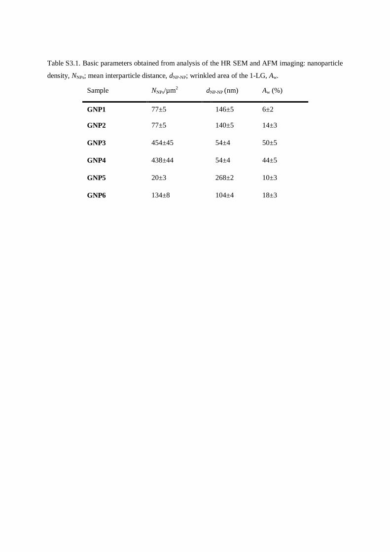
Table S3.1. Basic parameters obtained from analysis of the HR SEM and AFM imaging: nanoparticle
density, NNPs; mean interparticle distance, dNP-NP; wrinkled area of the 1-LG, Aw.
Sample NNPs/µm2 dNP-NP (nm) Aw (%)
GNP1 77±5 146±5 6±2
GNP2 77±5 140±5 14±3
GNP3 454±45 54±4 50±5
GNP4 438±44 54±4 44±5
GNP5 20±3 268±2 10±3
GNP6 134±8 104±4 18±3

Nanoparticle density; NNPs
/m2
0 100 200 300 400 500 600Re
lati
ve
de
lam
ina
ted
are
a, A
w (
%)
0
20
40
60
80
100
Mean interparticle distance; dNP-NP
(nm)
0 50 100 150 200 250 300
S3.3. Correlation of the mean nanoparticle density, NNPs (black) and mean interparticle distance, dNP-NP
(red) to relative delaminated area of 1-LG, Aw determined from AFM data. The Aw(NNPs)
dependence can be expressed as a linear function: Aw(NNPs) = a(NNPs) + b, where a =
0.094±0.009 and b = 4.8±2.4; the Aw(dNP-NP) dependence follows approximately a hyperbolic
function: Aw(dNP-NP) = c/(dNP-NP) + d, where c = 2964±389 and d = 7.6±4.6.

Nanoparticle density; NNPs
/m2
10 20 50 100 200 500
Rela
tive R
am
an
in
ten
sit
y o
f G
' 2;
I(G
' 2)/
I(G
' 1)
0.0
0.1
0.2
0.3
0.4
0.5
Mean particle distance; dNPs (nm)
50 100 150 200 250 300
0.0
0.1
0.2
0.3
0.4
0.5
S3.4. Correlation of the key parameters representing the spatial distribution of nanoparticles and level
of wrinkling of the 1-LG layer estimated from the analysis of the G’ mode (mean nanoparticle
density, NNPs (and mean interparticle distance, dNP-NP (red), relative area of wrinkles, Aw). The
dependencies do not show a clear monotonic trend as in case of the G mode-related features due to
complex structure of the G’ mode.

S.4 Profile analysis of the Raman spectra
The individual Raman peaks were fitted by the profile function ) (eq.S1) aproximated in the
form of the pseudo-Voigt function (linear combination of the Gaussian and Lorentizan as a sufficient
approximation of their convolution – Voigt function).The symbols used in equation S4.1 have the
following meaning: I - Raman intensity, - Raman shift, - peak position, - full width at half
maximum of the peak and - fraction of the Lorentzian component. The Gaussian component serves
as a measure of distribution of the peak parameters due to finite size of the laser spot (~1 m2), which
is expected to be about one order larger then the local variation of the parameters at nm scale.
(S4.1)
2
2
0
2
2
02
4
)(1
2
1
4
)(2lnexp
42ln)1(),(
III