Supplementary Appendix for Liquidity, Volume, and Price ...
20
Supplementary Appendix for Liquidity, Volume, and Price Behavior: The Impact of Order vs. Quote Based Trading –not for publication– Katya Malinova * University of Toronto Andreas Park † University of Toronto March 16, 2009 Abstract This document contains an extensive number of tables and graphs to support the numerical analysis in Sections 5 and 6 of the main text; these figures are num- bered consecutively following those in the main text. This document also provides additional information about the institutional background of trading mechanisms, technical details of the information structure used in the main text and, a detailed description of the simulation process that we employed to obtain our results in Section 8 of the main text. * Email: [email protected]; web: http://individual.utoronto.ca/kmalinova/. † Email: [email protected]; web: http://www.chass.utoronto.ca/∼apark/.
Transcript of Supplementary Appendix for Liquidity, Volume, and Price ...

Supplementary Appendix for
Liquidity, Volume, and Price Behavior:
The Impact of Order vs. Quote Based Trading
–not for publication–
Katya Malinova∗
University of Toronto
Andreas Park†
University of Toronto
March 16, 2009
Abstract
This document contains an extensive number of tables and graphs to support
the numerical analysis in Sections 5 and 6 of the main text; these figures are num-
bered consecutively following those in the main text. This document also provides
additional information about the institutional background of trading mechanisms,
technical details of the information structure used in the main text and, a detailed
description of the simulation process that we employed to obtain our results in
Section 8 of the main text.
∗Email: [email protected]; web: http://individual.utoronto.ca/kmalinova/.†Email: [email protected]; web: http://www.chass.utoronto.ca/∼apark/.

C Appendix: The Institutional Background
Our treatment of price formation in the dealer market is stylized: effectively, people sub-
mit their market orders without knowing the price and there are no standing quotes from
dealers. Of course, in real markets dealers do post quotes, but they usually quote only
a single bid and a single ask price. Moreover, for most markets, dealers are commonly
required to trade a guaranteed minimum number of units at this price (for instance,
on Nasdaq a quote‘must be “good” for 1000 shares for most stocks). Alternatively, on
exchanges such as the TSX or Paris Bourse, the upstairs dealers are required to trade at
the best bid or offer (BBO) that is currently on the book, unless the size of the trade is
very large. Finally, trading systems or exchanges that include small-order routing (i.e.
small orders are given to different dealers according to a pre-determined set of routing
rules) require dealers to do price improvement, that is they require dealers to give small
size orders the best price that is currently quoted.
None of these institutional details contradict our setup. First, the defining feature of
dealer markets is that the dealer will know the size of the trade when quoting the uniform
price for the order. Thus the dealer quotes cannot be ‘hit’ in the same way as a standing
limit order in a consolidated limit order book. Next, in the theoretical analysis of our
paper we describe that the dealer charges different prices for different quantities. The
bid- and ask-prices that she quotes would be for the minimum quantity that she must
trade — and this quantity may well be “large”; in other words, the quoted ask price may
be ask2
D, but when facing a small order, the dealer may offer ask1
D. Third, in our model
traders accurately anticipate the price that they will be quoted. Consequently, quotes
will be self-fulfilling. Finally, the BBO requirement in upstairs-downstairs markets is
trivially satisfied in the hybrid market.
D Appendix: Quality and Belief Distributions
Financial market microstructure models with binary signals and states typically employ
a constant signal quality q ∈ [1/2, 1], with Pr(S = v|V = v) = q. Our framework has
a continuum of possible qualities with a continuous density function and, as outlined
above, we will map investors’ signals and their qualities into a continuous private belief
on [0, 1]. The quality parametrization on [1/2, 1] is very natural, as a trader who receives
a high signal h will update his prior in favor of the high liquidation value, V = 1, and a
trader who receives a low signal l will update his prior in favor of V = 0. We thus use
the conventional parametrization on [1/2, 1] in the main text.
1 Appendix for Trading Mechanisms & Market Dynamics
However, to characterize the map from investors’ signal and qualities into their pri-
vate beliefs and to derive the distributions of the latter, it is mathematically convenient
to normalize the signal quality so that its domain coincides with that of the private
belief. We will denote the distribution function of this normalized quality on [0, 1] by G
and its density by g, whereas the distribution and density functions of original qualities
on [1/2, 1] will be denoted by G̃ and g̃ respectively.
The normalization proceeds as follows. Without loss of generality, we will employ
the density function g that is symmetric around 1/2. For q ∈ [0, 1/2], we then have
g(q) = g̃(1 − q)/2 and for q ∈ [1/2, 1], we have g(q) = g̃(q)/2.
Under this specification, signal qualities q and 1−q are equally useful for the individ-
ual: if someone receives signal h and has quality 1/4, then this signal has ‘the opposite
meaning’, i.e. it has the same meaning as receiving signal l with quality 3/4. Signal
qualities are assumed to be independent across agents, and independent of the security’s
liquidation value V .
Beliefs are derived by Bayes Rule, given signals and signal-qualities. Specifically, if
a trader is told that his signal quality is q and receives a high signal h then his belief
is q/[q + (1 − q)] = q (respectively 1 − q if he receives a low signal l), because the prior
is 1/2. The belief π is thus held by people who receive signal h and quality q = π and by
those who receive signal l and quality q = 1−π. Consequently, the density of individuals
with belief π is given by f1(π) = π[g(π) + g(1 − π)] in state V = 1 and analogously by
f0(π) = (1 − π)[g(π) + g(1 − π)] in state V = 0.
Smith and Sorensen (2008) prove the following property of private beliefs (Lemma 2
in their paper):
Lemma 1 (Symmetric beliefs, Smith and Sorensen (2008))
With the above the signal quality structure, private belief distributions satisfy F1(π) =
1 − F0(1 − π) for all π ∈ (0, 1).
Proof: Since f1(π) = π[g(π) + g(1 − π)] and f0(π) = (1 − π)[g(π) + g(1 − π)], we have
f1(π) = f0(1 − π). Integrating, F1(π) =∫ π
0f1(x)dx =
∫ π
0f0(1 − x)dx =
∫1
1−πf0(x)dx =
1 − F0(1 − π). �
A direct implication of this lemma is that with symmetric thresholds, πb = 1− πs, a
buy in state V = 1 is as likely as a sale in state V = 0, because
β1 = (1− µ)/2 + µ(1− F1(πb)) = (1− µ)/2 + µF0(1− πbb) = (1− µ)/2 + µF0(πs) = σ0.
Similarly, β0 = σ1. Next, the belief densities satisfy the monotone likelihood ratio
2 Appendix for Trading Mechanisms & Market Dynamics

property becausef1(π)
f0(π)=
π[g(π) + g(1 − π)]
(1 − π)[g(π) + g(1 − π)]=
π
1 − π
is increasing in π.
One can recover the distribution of qualities on [1/2, 1], denoted by G̃, from G by
combining qualities that yield the same beliefs for opposing signals (e.g q = 1/4 and
signal h is combined with q = 3/4 and signal l). With symmetric g, G(1/2) = 1/2, and
G̃(q) =
∫ q
1
2
g(s)ds +
∫ 1
2
1−q
g(s)ds = 2
∫ q
1
2
g(s)ds = 2G(q) − 2G(1/2) = 2G(q) − 1. (1)
E Simulation Procedure for Price Efficiency
We employed the following data generation procedure for the simulations: We ob-
tained 500,000 observations of trading days for each of the Poisson arrival rates ρ ∈
{5, 10, 15, 20, 25, 30, 35, 40, 45, 50} and levels of informed trading µ ∈ {.1, .2, .3, .4, .5, .6,
.7, .8, .9}. Here, the Poisson arrival rate ρ implies that, on average, there are ρ traders
(though some may choose not to trade). Fixing the true value to V = 1, prices are closer
to the true value if they are larger. To get a better sense of the effect of a small ρ for
transparent vs. opaque hybrid markets, we also ran ρ ∈ {1, 2, . . . , 14} for µ ∈ {.2, .5, .8},
as outlined in the main text.
For each series, we first drew the number of traders for the session and performed
the random allocation of traders into noise and informed. Thus overall there were, for
instance, approximately 25,000,000 trades for ρ = 50. The informed traders were then
equipped with a signal quality and a draw of the high or low signal for that quality,
conditional on V = 1. Noise traders were assigned a random trading role. We then
determined a random entry order and for the hybrid market performed an additional
random draw to determine in which market the respective trader will be placing this
order. Finally, we computed the end-prices that would result for each trading sessions
under each of the four trading regimes. One can think of these prices at the prices that
would obtain at the end of a trading day. Our results are for the distribution of these
final prices. Our descriptions on properties of the empirical distributions are based on
the case with ρ = 50. The rule of thumb is that the larger is ρ, the diverse the outcomes
of trading rounds are and the closer are the distributions of end prices to a smooth
continuous function (for small values of ρ they resemble step functions).
3 Appendix for Trading Mechanisms & Market Dynamics
mu
Ask
(lim
it)-A
sk(hyb
rid)
0.005
0.010
0.015
0.020
mu
Ask(hyb
rid)-A
sk(dealer)
0.01
0.02
0.03
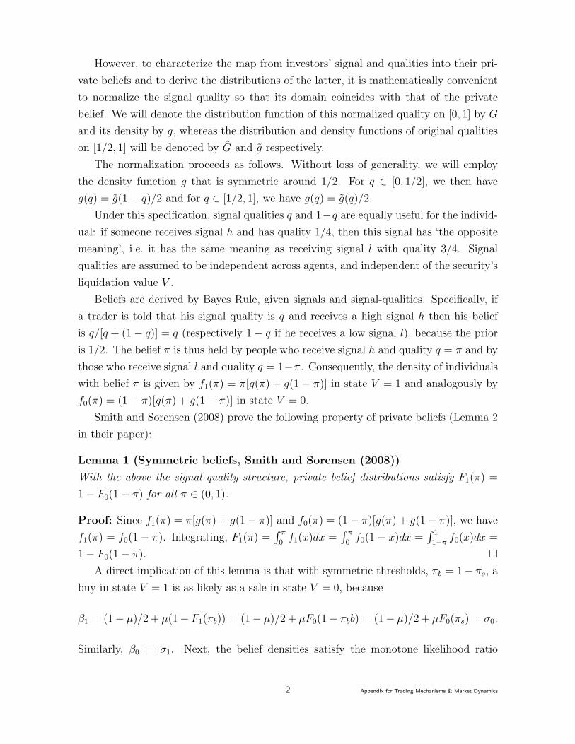
Figure 4: Bid-Ask-Spreads in Limit Order, Dealer and Hybrid Markets. In each panel a lineplots a difference of ask-prices under specific market mechanisms as a function of the amount informedtrading, µ, for a specific prior p. The left panel plots the difference of ask prices for the first unit inthe limit order and hybrid markets, the right plots the difference of ask prices for small trades in thehybrid and dealer markets. The panels illustrate Proposition 3 (a).
References
Smith, L., and P. Sorensen (2008): “Rational Social Learning with Random Sam-
pling,” mimeo, University of Michigan.
4 Appendix for Trading Mechanisms & Market Dynamics
m
Cos
t(lim
it)-C
ost(hy
brid)
K0.0150
K0.0125
K0.0100
K0.0075
K0.0050
K0.0025
m
Cos
t(hy
brid)-Cos
t(de
aler)
K0.03
K0.02
K0.01
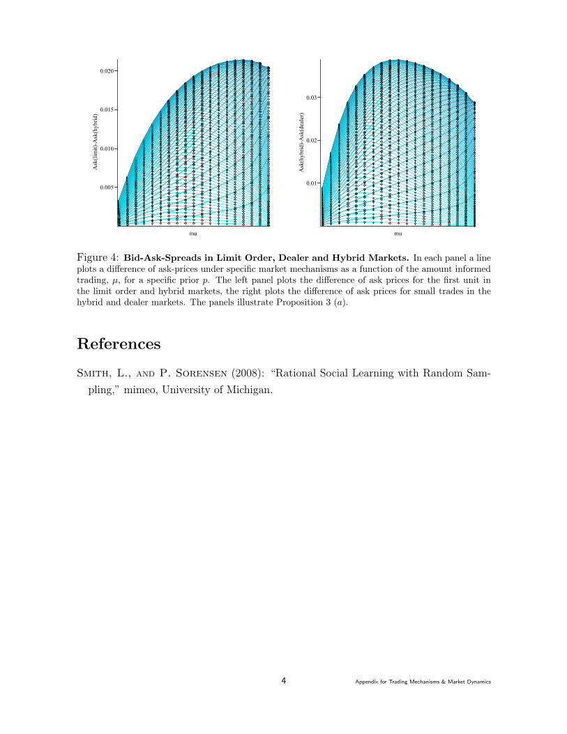
Figure 5: Execution Costs for Large Orders in Limit Order, Dealer and Hybrid Markets. Ineach panel a line plots a difference of execution costs for larger orders under specific market mechanismsas a function of the amount informed trading, µ, for a specific prior p. The left panel plots the costdifference in limit order market and the hybrid market, the right panel plots the cost difference for thehybrid market and the dealer market. The panels illustrate Proposition 3 (b).
m
Impa
ct(l
imit)
-Im
pact
(hyb
rid
limit)
K0.15
K0.10
K0.05
m
Impa
ct(h
ybri
d lim
it)-I
mpa
ct(d
eale
r)
K0.25
K0.20
K0.15
K0.10
K0.05
Figure 6: Price Impacts of Small Trades in Limit Order, Dealer and Hybrid Markets. Ineach panel a line plots a difference of price impacts of small orders under specific market mechanisms asa function of the amount informed trading, µ, for a specific prior p. The left panel plots the difference ofprice impacts of small orders in the limit order market and the hybrid market, the right panel plots thedifference of price impacts of small orders in the limit order segment of the hybrid market and isolateddealer market. As ask
1
H > ask1
D by part (a), the panels illustrate Proposition 3 (c).
5 Appendix for Trading Mechanisms & Market Dynamics
m
Impa
ct(h
ybri
d lim
it)-I
mpa
ct(l
imit)
, lar
ge tr
ades
0.01
0.02
0.03
m
Impa
ct(d
eale
r)-I
mpa
ct(h
ybri
d de
aler
), la
rge
trad
es
0.005
0.010
0.015
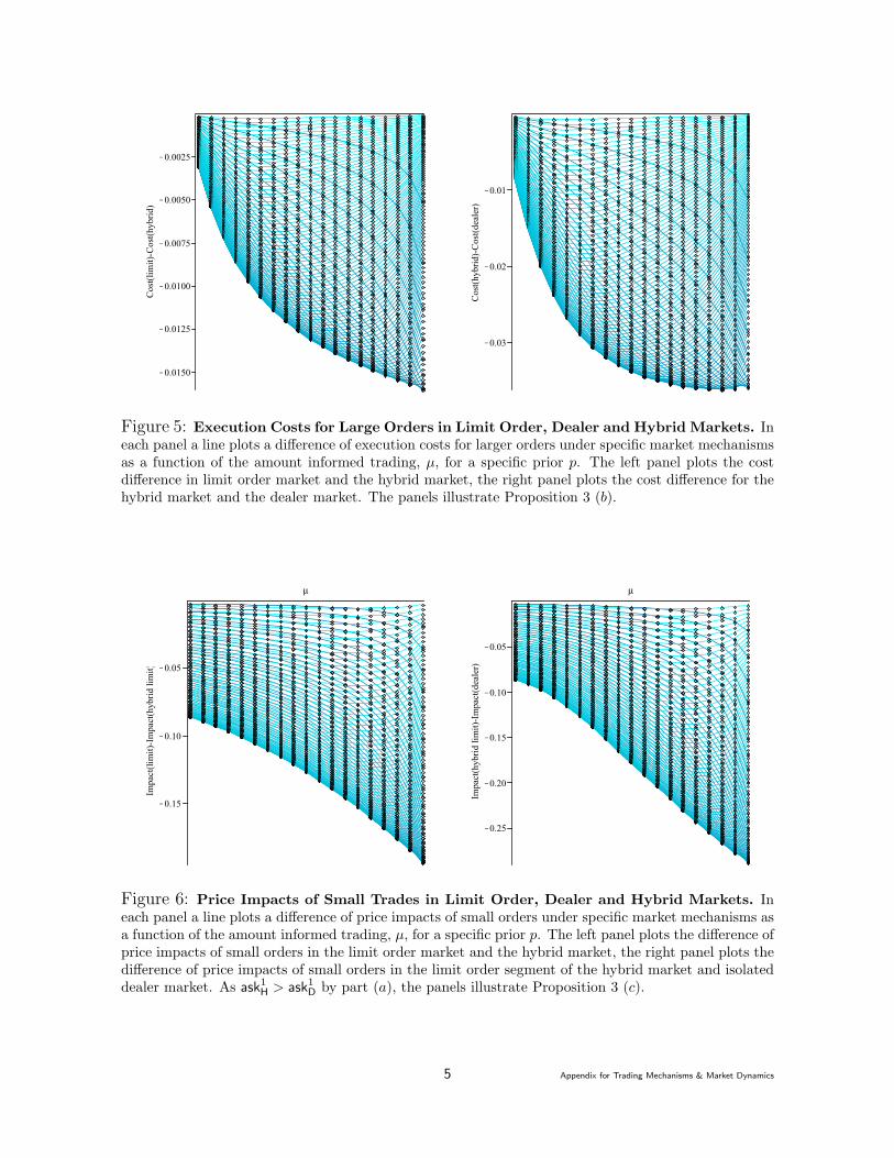
Figure 7: Price Impacts of Large Trades in Limit Order, Dealer and Hybrid Markets. Ineach panel a line plots a difference of price impacts of large orders under specific market mechanisms asa function of the amount informed trading, µ, for a specific prior p. The left panel plots the differenceof price impacts of large orders in the limit order segment of the hybrid market and the isolated limitorder market market, the right panel plots the difference of price impacts of large orders in the isolateddealer market and the dealer segment of the hybrid market. The panels illustrate Proposition 3 (c).
m
Volum
e(lim
it)-V
olum
e(hy
brid)
0.0025
0.0050
0.0075
0.0100
0.0125
m
Volum
e(hy
brid)-Volum
e(de
aler)
0.01
0.02
0.03
Figure 8: Volume in Limit Order, Dealer and Hybrid Markets. In each panel a line plots adifference of volume under specific market mechanisms as a function of the amount informed trading,µ, for a specific prior p. The first panel plots the difference of volume in limit order and hybrid markets,the second plots the difference of volume in hybrid and dealer markets. Both cleanly indicate the orderexpressed in Numerical Observation 1.
6 Appendix for Trading Mechanisms & Market Dynamics

Closing Price Limit Order Market - Dealer Market5 10 15 20 25 30 35 40 45 50
0.1 0.0003 0.0006 0.0009 0.0012 0.0014 0.0016 0.0019 0.0020 0.0022 0.0024+ + + + + + + + + +
0.2 0.0029 0.0051 0.0069 0.0083 0.0095 0.0104 0.0111 0.0116 0.0120 0.0125+ + + + + + + + + +
0.3 0.0074 0.0119 0.0148 0.0170 0.0180 0.0188 0.0192 0.0193 0.0189 0.0186+ + + + + + + + + +
0.4 0.0116 0.0170 0.0198 0.0207 0.0207 0.0205 0.0194 0.0185 0.0171 0.0159+ + + + + + + + + +
0.5 0.0132 0.0180 0.0193 0.0191 0.0178 0.0161 0.0145 0.0125 0.0110 0.0096+ + + + + + + + + +
0.6 0.0121 0.0150 0.0145 0.0135 0.0117 0.0096 0.0079 0.0064 0.0052 0.0043+ + + + + + + + + +
0.7 0.0076 0.0090 0.0086 0.0070 0.0053 0.0042 0.0033 0.0024 0.0019 0.0014+ + + + + + + + + +
0.8 0.0014 0.0019 0.0017 0.0013 0.0011 0.0008 0.0005 0.0003 0.0002 0.0002+ + + + + + + + + +
0.9 -0.0081 -0.0062 -0.0045 -0.0032 -0.0019 -0.0013 -0.0008 -0.0004 -0.0003 -0.0002- - - - - - - - - -
Table 1: Difference of Average Closing Prices: Limit Order vs. Dealer Market. Thistable is based upon the simulations described in the main text. Columns denote the entry rateρ, rows the level of informed trading µ. Thus each entry denotes the difference of the averageclosing prices in Limit Order and Dealer markets for a specific (ρ, µ)-combination. As theunderlying true value is V = 1, the higher a price is, the closer it is to the true value and thusthe more efficient it is. Thus a positive difference of the average closing prices indicates thatthe Limit Order Market is more efficient. As the table indicates, this is always the case butfor the largest values of µ that we considered. This table relates to Numerical Observation 2.
7 Appendix for Trading Mechanisms & Market Dynamics
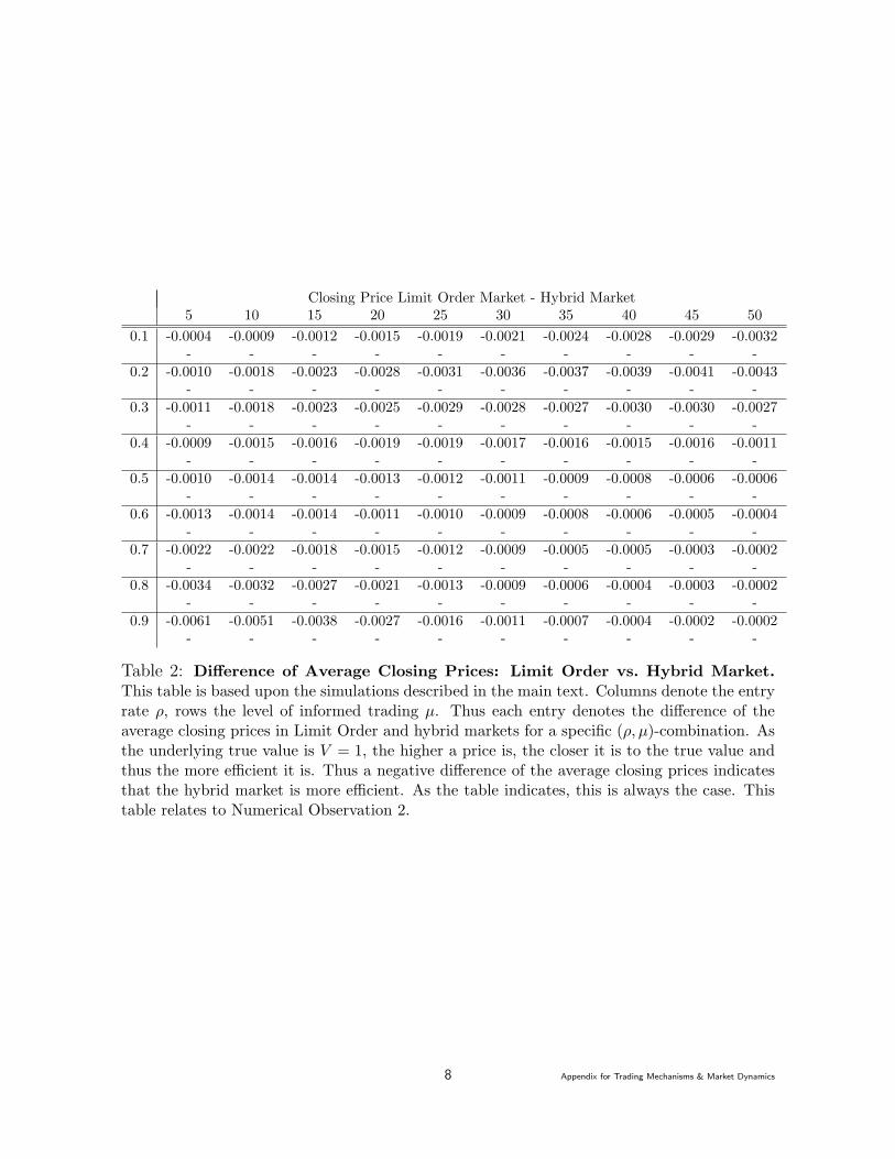
Closing Price Limit Order Market - Hybrid Market5 10 15 20 25 30 35 40 45 50
0.1 -0.0004 -0.0009 -0.0012 -0.0015 -0.0019 -0.0021 -0.0024 -0.0028 -0.0029 -0.0032- - - - - - - - - -
0.2 -0.0010 -0.0018 -0.0023 -0.0028 -0.0031 -0.0036 -0.0037 -0.0039 -0.0041 -0.0043- - - - - - - - - -
0.3 -0.0011 -0.0018 -0.0023 -0.0025 -0.0029 -0.0028 -0.0027 -0.0030 -0.0030 -0.0027- - - - - - - - - -
0.4 -0.0009 -0.0015 -0.0016 -0.0019 -0.0019 -0.0017 -0.0016 -0.0015 -0.0016 -0.0011- - - - - - - - - -
0.5 -0.0010 -0.0014 -0.0014 -0.0013 -0.0012 -0.0011 -0.0009 -0.0008 -0.0006 -0.0006- - - - - - - - - -
0.6 -0.0013 -0.0014 -0.0014 -0.0011 -0.0010 -0.0009 -0.0008 -0.0006 -0.0005 -0.0004- - - - - - - - - -
0.7 -0.0022 -0.0022 -0.0018 -0.0015 -0.0012 -0.0009 -0.0005 -0.0005 -0.0003 -0.0002- - - - - - - - - -
0.8 -0.0034 -0.0032 -0.0027 -0.0021 -0.0013 -0.0009 -0.0006 -0.0004 -0.0003 -0.0002- - - - - - - - - -
0.9 -0.0061 -0.0051 -0.0038 -0.0027 -0.0016 -0.0011 -0.0007 -0.0004 -0.0002 -0.0002- - - - - - - - - -
Table 2: Difference of Average Closing Prices: Limit Order vs. Hybrid Market.
This table is based upon the simulations described in the main text. Columns denote the entryrate ρ, rows the level of informed trading µ. Thus each entry denotes the difference of theaverage closing prices in Limit Order and hybrid markets for a specific (ρ, µ)-combination. Asthe underlying true value is V = 1, the higher a price is, the closer it is to the true value andthus the more efficient it is. Thus a negative difference of the average closing prices indicatesthat the hybrid market is more efficient. As the table indicates, this is always the case. Thistable relates to Numerical Observation 2.
8 Appendix for Trading Mechanisms & Market Dynamics
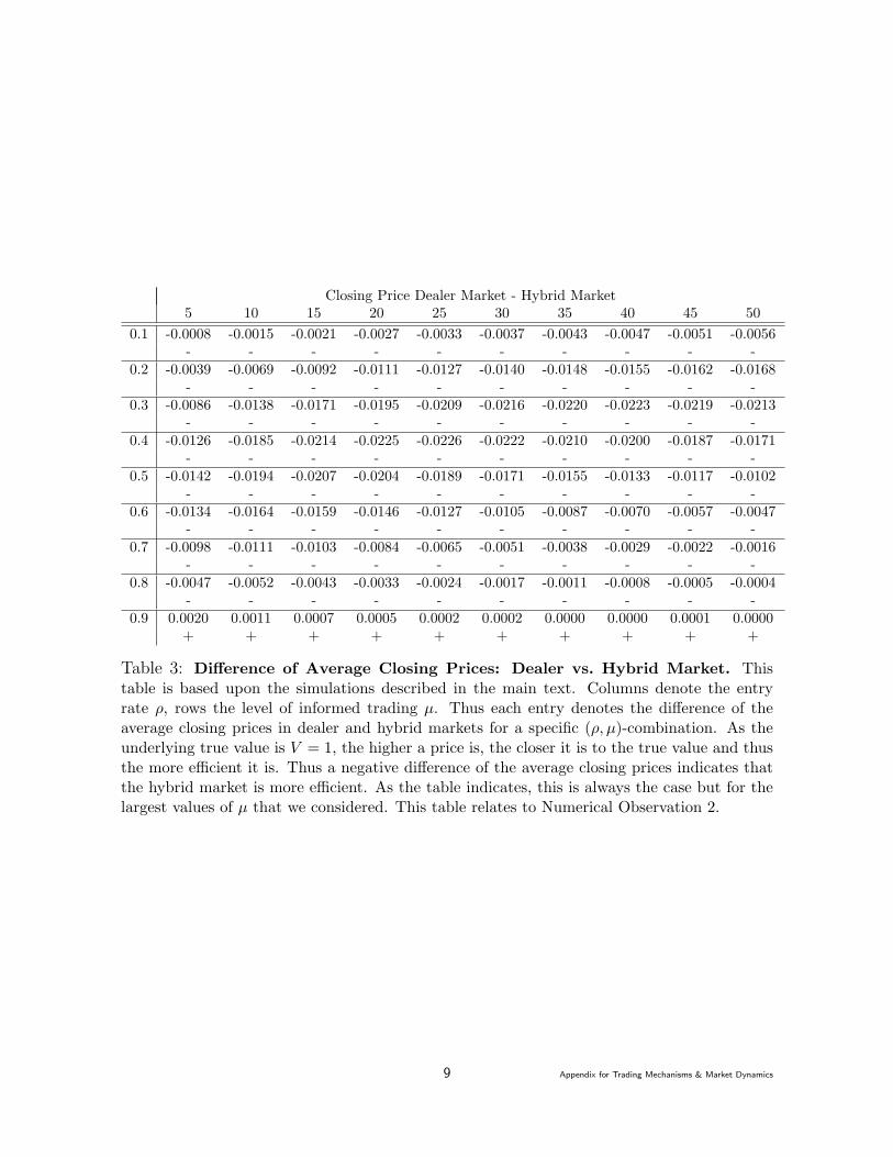
Closing Price Dealer Market - Hybrid Market5 10 15 20 25 30 35 40 45 50
0.1 -0.0008 -0.0015 -0.0021 -0.0027 -0.0033 -0.0037 -0.0043 -0.0047 -0.0051 -0.0056- - - - - - - - - -
0.2 -0.0039 -0.0069 -0.0092 -0.0111 -0.0127 -0.0140 -0.0148 -0.0155 -0.0162 -0.0168- - - - - - - - - -
0.3 -0.0086 -0.0138 -0.0171 -0.0195 -0.0209 -0.0216 -0.0220 -0.0223 -0.0219 -0.0213- - - - - - - - - -
0.4 -0.0126 -0.0185 -0.0214 -0.0225 -0.0226 -0.0222 -0.0210 -0.0200 -0.0187 -0.0171- - - - - - - - - -
0.5 -0.0142 -0.0194 -0.0207 -0.0204 -0.0189 -0.0171 -0.0155 -0.0133 -0.0117 -0.0102- - - - - - - - - -
0.6 -0.0134 -0.0164 -0.0159 -0.0146 -0.0127 -0.0105 -0.0087 -0.0070 -0.0057 -0.0047- - - - - - - - - -
0.7 -0.0098 -0.0111 -0.0103 -0.0084 -0.0065 -0.0051 -0.0038 -0.0029 -0.0022 -0.0016- - - - - - - - - -
0.8 -0.0047 -0.0052 -0.0043 -0.0033 -0.0024 -0.0017 -0.0011 -0.0008 -0.0005 -0.0004- - - - - - - - - -
0.9 0.0020 0.0011 0.0007 0.0005 0.0002 0.0002 0.0000 0.0000 0.0001 0.0000+ + + + + + + + + +
Table 3: Difference of Average Closing Prices: Dealer vs. Hybrid Market. Thistable is based upon the simulations described in the main text. Columns denote the entryrate ρ, rows the level of informed trading µ. Thus each entry denotes the difference of theaverage closing prices in dealer and hybrid markets for a specific (ρ, µ)-combination. As theunderlying true value is V = 1, the higher a price is, the closer it is to the true value and thusthe more efficient it is. Thus a negative difference of the average closing prices indicates thatthe hybrid market is more efficient. As the table indicates, this is always the case but for thelargest values of µ that we considered. This table relates to Numerical Observation 2.
9 Appendix for Trading Mechanisms & Market Dynamics

−.0
2−
.01
0.0
1.0
2.0
3cd
f(de
aler
)−cd
f(LO
B)
0 .2 .4 .6 .8 1price
FOSD dealer vs LOB
−.0
20
.02
.04
.06
cdf(
deal
er)−
cdf(
LOB
)
0 .2 .4 .6 .8 1price
FOSD dealer vs LOB
0.0
2.0
4.0
6.0
8cd
f(de
aler
)−cd
f(LO
B)
0 .2 .4 .6 .8 1price
FOSD dealer vs LOB
µ = .1 µ = .2 µ = .3
0.0
2.0
4.0
6.0
8.1
cdf(
deal
er)−
cdf(
LOB
)
0 .2 .4 .6 .8 1price
FOSD dealer vs LOB
0.0
5.1
cdf(
deal
er)−
cdf(
LOB
)
0 .2 .4 .6 .8 1price
FOSD dealer vs LOB
0.0
2.0
4.0
6.0
8.1
cdf(
deal
er)−
cdf(
LOB
)
0 .2 .4 .6 .8 1price
FOSD dealer vs LOB
µ = .4 µ = .5 µ = .6
0.0
1.0
2.0
3.0
4.0
5cd
f(de
aler
)−cd
f(LO
B)
0 .2 .4 .6 .8 1price
FOSD dealer vs LOB
0.0
05.0
1.0
15.0
2cd
f(de
aler
)−cd
f(LO
B)
0 .2 .4 .6 .8 1price
FOSD dealer vs LOB
−.0
04−
.003
−.0
02−
.001
0.0
01cd
f(de
aler
)−cd
f(LO
B)
0 .2 .4 .6 .8 1price
FOSD dealer vs LOB
µ = .7 µ = .8 µ = .9
Figure 9: First Order Stochastic Dominance of Closing Prices Dealer Market vs. Limit
Order Book. The panels plot differences of empirical distributions as a functions of the price FD(p)−FL(p) and illustrates Numerical Observation 3 (a).
10 Appendix for Trading Mechanisms & Market Dynamics
−.0
20
.02
.04
cdf(
deal
er)−
cdf(
hybr
id)
0 .2 .4 .6 .8 1price
FOSD dealer vs hybrid
−.0
20
.02
.04
.06
cdf(
deal
er)−
cdf(
LOB
)
0 .2 .4 .6 .8 1price
FOSD dealer vs LOB
0.0
2.0
4.0
6.0
8cd
f(de
aler
)−cd
f(LO
B)
0 .2 .4 .6 .8 1price
FOSD dealer vs LOB
µ = .1 µ = .2 µ = .3
0.0
2.0
4.0
6.0
8.1
cdf(
deal
er)−
cdf(
hybr
id)
0 .2 .4 .6 .8 1price
FOSD dealer vs hybrid
0.0
5.1
.15
cdf(
deal
er)−
cdf(
hybr
id)
0 .2 .4 .6 .8 1price
FOSD dealer vs hybrid
0.0
2.0
4.0
6.0
8.1
cdf(
deal
er)−
cdf(
hybr
id)
0 .2 .4 .6 .8 1price
FOSD dealer vs hybrid
µ = .4 µ = .5 µ = .6
0.0
2.0
4.0
6cd
f(de
aler
)−cd
f(hy
brid
)
0 .2 .4 .6 .8 1price
FOSD dealer vs hybrid
0.0
05.0
1.0
15.0
2cd
f(de
aler
)−cd
f(hy
brid
)
0 .2 .4 .6 .8 1price
FOSD dealer vs hybrid
0.0
01.0
02.0
03cd
f(de
aler
)−cd
f(hy
brid
)
0 .2 .4 .6 .8 1price
FOSD dealer vs hybrid
µ = .7 µ = .8 µ = .9
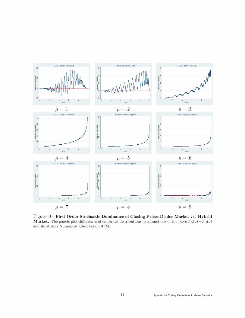
Figure 10: First Order Stochastic Dominance of Closing Prices Dealer Market vs. Hybrid
Market. The panels plot differences of empirical distributions as a functions of the price FD(p)−FH(p)and illustrates Numerical Observation 3 (b).
11 Appendix for Trading Mechanisms & Market Dynamics
−.0
4−
.02
0.0
2.0
4cd
f(LO
B)−
cdf(
hybr
id)
0 .2 .4 .6 .8 1price
FOSD LOB vs hybrid
−.0
10
.01
.02
.03
cdf(
LOB
)−cd
f(hy
brid
)
0 .2 .4 .6 .8 1price
FOSD LOB vs hybrid
−.0
050
.005
.01
.015
.02
cdf(
LOB
)−cd
f(hy
brid
)
0 .2 .4 .6 .8 1price
FOSD LOB vs hybrid
µ = .1 µ = .2 µ = .3
0.0
05.0
1cd
f(LO
B)−
cdf(
hybr
id)
0 .2 .4 .6 .8 1price
FOSD LOB vs hybrid
0.0
02.0
04.0
06.0
08.0
1cd
f(LO
B)−
cdf(
hybr
id)
0 .2 .4 .6 .8 1price
FOSD LOB vs hybrid
0.0
01.0
02.0
03.0
04.0
05cd
f(LO
B)−
cdf(
hybr
id)
0 .2 .4 .6 .8 1price
FOSD LOB vs hybrid
µ = .4 µ = .5 µ = .6
0.0
02.0
04.0
06cd
f(LO
B)−
cdf(
hybr
id)
0 .2 .4 .6 .8 1price
FOSD LOB vs hybrid
0.0
01.0
02.0
03.0
04cd
f(LO
B)−
cdf(
hybr
id)
0 .2 .4 .6 .8 1price
FOSD LOB vs hybrid
0.0
02.0
04.0
06cd
f(LO
B)−
cdf(
hybr
id)
0 .2 .4 .6 .8 1price
FOSD LOB vs hybrid
µ = .7 µ = .8 µ = .9
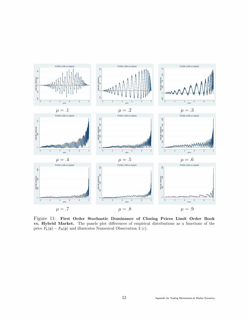
Figure 11: First Order Stochastic Dominance of Closing Prices Limit Order Book
vs. Hybrid Market. The panels plot differences of empirical distributions as a functions of theprice FL(p) − FH(p) and illustrates Numerical Observation 3 (c).
12 Appendix for Trading Mechanisms & Market Dynamics

010
2030
ccdf
(dea
ler)
−cc
df(L
OB
)
0 .2 .4 .6 .8 1price
SOSD dealer vs LOB
050
100
150
ccdf
(dea
ler)
−cc
df(L
OB
)
0 .2 .4 .6 .8 1price
SOSD dealer vs LOB
050
100
150
200
ccdf
(dea
ler)
−cc
df(L
OB
)
0 .2 .4 .6 .8 1price
SOSD dealer vs LOB
µ = .1 µ = .2 µ = .3
050
100
150
ccdf
(dea
ler)
−cc
df(L
OB
)
0 .2 .4 .6 .8 1price
SOSD dealer vs LOB
020
4060
8010
0cc
df(d
eale
r)−
ccdf
(LO
B)
0 .2 .4 .6 .8 1price
SOSD dealer vs LOB
010
2030
40cc
df(d
eale
r)−
ccdf
(LO
B)
0 .2 .4 .6 .8 1price
SOSD dealer vs LOB
µ = .4 µ = .5 µ = .6
05
1015
ccdf
(dea
ler)
−cc
df(L
OB
)
0 .2 .4 .6 .8 1price
SOSD dealer vs LOB
0.5
11.
5cc
df(d
eale
r)−
ccdf
(LO
B)
0 .2 .4 .6 .8 1price
SOSD dealer vs LOB
−.0
04−
.003
−.0
02−
.001
0.0
01cd
f(de
aler
)−cd
f(LO
B)
0 .2 .4 .6 .8 1price
FOSD dealer vs LOB
µ = .7 µ = .8 µ = .9
Figure 12: Second Order Stochastic Dominance of Closing Prices Dealer Market vs. Limit
Order Book. The panels plot differences of empirical distributions as a functions of the price∫ p
0[FD(s)−
FL(s)]ds and illustrates Numerical Observation 4 (a).
13 Appendix for Trading Mechanisms & Market Dynamics
−20
020
4060
ccdf
(dea
ler)
−cc
df(h
ybrid
)
0 .2 .4 .6 .8 1price
SOSD dealer vs hybrid
050
100
150
200
ccdf
(dea
ler)
−cc
df(h
ybrid
)
0 .2 .4 .6 .8 1price
SOSD dealer vs hybrid
050
100
150
200
ccdf
(dea
ler)
−cc
df(L
OB
)
0 .2 .4 .6 .8 1price
SOSD dealer vs LOB
µ = .1 µ = .2 µ = .3
050
100
150
200
ccdf
(dea
ler)
−cc
df(h
ybrid
)
0 .2 .4 .6 .8 1price
SOSD dealer vs hybrid
020
4060
8010
0cc
df(d
eale
r)−
ccdf
(hyb
rid)
0 .2 .4 .6 .8 1price
SOSD dealer vs hybrid
010
2030
4050
ccdf
(dea
ler)
−cc
df(h
ybrid
)
0 .2 .4 .6 .8 1price
SOSD dealer vs hybrid
µ = .4 µ = .5 µ = .6
05
1015
ccdf
(dea
ler)
−cc
df(h
ybrid
)
0 .2 .4 .6 .8 1price
SOSD dealer vs hybrid
01
23
4cc
df(d
eale
r)−
ccdf
(hyb
rid)
0 .2 .4 .6 .8 1price
SOSD dealer vs hybrid
−.4
−.3
−.2
−.1
0cc
df(d
eale
r)−
ccdf
(hyb
rid)
0 .2 .4 .6 .8 1price
SOSD dealer vs hybrid
µ = .7 µ = .8 µ = .9
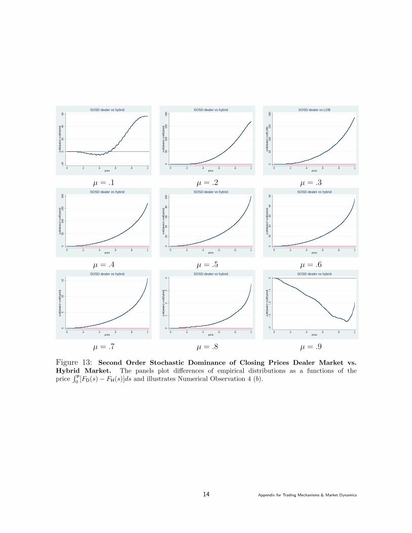
Figure 13: Second Order Stochastic Dominance of Closing Prices Dealer Market vs.
Hybrid Market. The panels plot differences of empirical distributions as a functions of theprice
∫ p
0[FD(s) − FH(s)]ds and illustrates Numerical Observation 4 (b).
14 Appendix for Trading Mechanisms & Market Dynamics
−10
010
2030
ccdf
(LO
B)−
ccdf
(hyb
rid)
0 .2 .4 .6 .8 1price
SOSD LOB vs. Hybrid
010
2030
40cc
df(L
OB
)−cc
df(h
ybrid
)
0 .2 .4 .6 .8 1price
SOSD LOB vs. hybrid
010
2030
ccdf
(LO
B)−
ccdf
(hyb
rid)
0 .2 .4 .6 .8 1price
SOSD LOB vs. Hybrid
µ = .1 µ = .2 µ = .3
05
10cc
df(L
OB
)−cc
df(h
ybrid
)
0 .2 .4 .6 .8 1price
SOSD LOB vs. Hybrid
02
46
ccdf
(LO
B)−
ccdf
(hyb
rid)
0 .2 .4 .6 .8 1price
SOSD LOB vs. Hybrid
01
23
4cc
df(L
OB
)−cc
df(h
ybrid
)
0 .2 .4 .6 .8 1price
SOSD LOB vs. Hybrid
µ = .4 µ = .5 µ = .6
0.5
11.
52
ccdf
(LO
B)−
ccdf
(hyb
rid)
0 .2 .4 .6 .8 1price
SOSD LOB vs. Hybrid
0.5
11.
52
ccdf
(LO
B)−
ccdf
(hyb
rid)
0 .2 .4 .6 .8 1price
SOSD LOB vs. Hybrid
0.5
11.
52
ccdf
(LO
B)−
ccdf
(hyb
rid)
0 .2 .4 .6 .8 1price
SOSD LOB vs. Hybrid
µ = .7 µ = .8 µ = .9
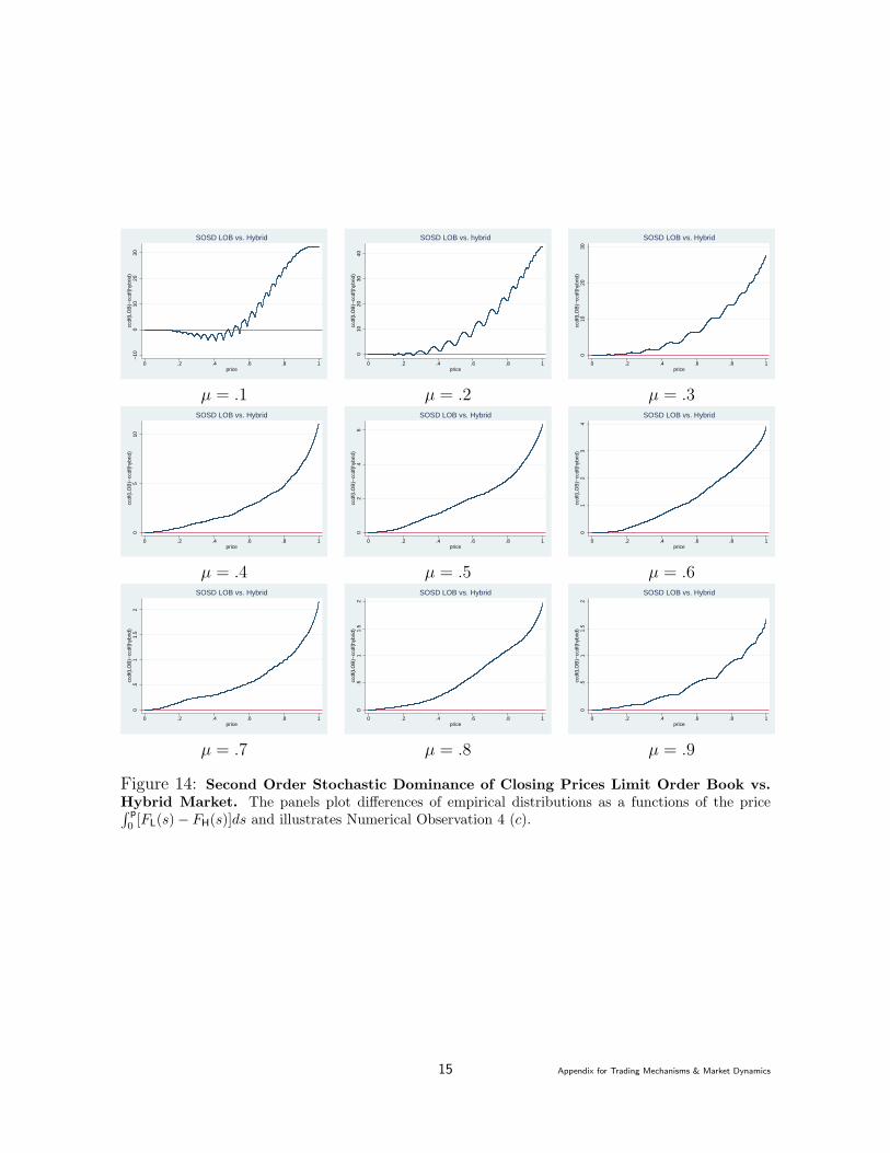
Figure 14: Second Order Stochastic Dominance of Closing Prices Limit Order Book vs.
Hybrid Market. The panels plot differences of empirical distributions as a functions of the price∫ p
0[FL(s) − FH(s)]ds and illustrates Numerical Observation 4 (c).
15 Appendix for Trading Mechanisms & Market Dynamics

Closing Price Hybrid Transparent - Hybrid Opaque5 10 15 20 25 30 35 40 45 50
0.1 0.0000 0.0001 0.0000 0.0003 0.0004 0.0006 0.0007 0.0011 0.0013 0.0013- + + + + + + + + +
0.2 0.0002 0.0007 0.0012 0.0022 0.0029 0.0038 0.0045 0.0050 0.0056 0.0062+ + + + + + + + + +
0.3 0.0001 0.0012 0.0027 0.0041 0.0052 0.0060 0.0072 0.0077 0.0079 0.0081+ + + + + + + + + +
0.4 -0.0001 0.0019 0.0037 0.0050 0.0060 0.0066 0.0071 0.0071 0.0068 0.0065- + + + + + + + + +
0.5 -0.0003 0.0018 0.0039 0.0049 0.0055 0.0054 0.0053 0.0045 0.0044 0.0040- + + + + + + + + +
0.6 -0.0011 0.0016 0.0029 0.0037 0.0038 0.0034 0.0031 0.0026 0.0022 0.0019- + + + + + + + + +
0.7 -0.0017 0.0006 0.0019 0.0022 0.0021 0.0019 0.0015 0.0012 0.0009 0.0007- + + + + + + + + +
0.8 -0.0027 -0.0003 0.0007 0.0010 0.0009 0.0008 0.0006 0.0004 0.0003 0.0002- - + + + + + + + +
0.9 -0.0034 -0.0014 -0.0003 0.0001 0.0002 0.0002 0.0002 0.0001 0.0001 0.0001- - - + + + + + + +
Table 4: Difference of Average Closing Prices: Transparent vs. Opaque Hybrid
Market. This table is based upon the simulations described in the main text. Columnsdenote the entry rate ρ, rows the level of informed trading µ. Thus each entry denotes thedifference of the average closing prices in transparent and opaque hybrid markets for a specific(ρ, µ)-combination. As the underlying true value is V = 1, the higher a price is, the closer itis to the true value and thus the more efficient it is. Thus a positive difference of the averageclosing prices indicates that the transparent hybrid market is more efficient. As the tableindicates, this is always the case but for small values of ρ that we considered; see also Table 5.This table support Numerical Observation 5 (a).
16 Appendix for Trading Mechanisms & Market Dynamics

Closing Price Hybrid Transparent - Hybrid Opaque for small rho1 2 3 4 5 6 7
0.2 -0.0001 -0.0001 0.0000 0.0000 0.0001 0.0002 0.0003- - + - + + +
0.5 -0.0009 -0.0011 -0.0011 -0.0010 -0.0005 -0.0001 0.0006- - - - - - +
0.8 -0.0028 -0.0035 -0.0035 -0.0031 -0.0026 -0.0021 -0.0017- - - - - - -
8 9 10 11 12 13 14
0.2 0.0002 0.0005 0.0006 0.0009 0.0009 0.0011 0.0012+ + + + + + +
0.5 0.0009 0.0015 0.0019 0.0025 0.0029 0.0031 0.0034+ + + + + + +
0.8 -0.0012 -0.0008 -0.0005 0.0000 0.0002 0.0003 0.0007- - - - + + +
Table 5: Difference of Average Closing Prices: Transparent vs. Opaque Hybrid
Market — small values of ρ. This table complements Table 5 and considers small valuesof ρ. is based upon the simulations described in the main text. Columns denote the entry rateρ, rows the level of informed trading µ. Thus each entry denotes the difference of the averageclosing prices in transparent and opaque hybrid markets for a specific (ρ, µ)-combination. Asthe underlying true value is V = 1, the higher a price is, the closer it is to the true value andthus the more efficient it is. Thus a positive difference of the average closing prices indicatesthat the transparent hybrid market is more efficient. As the table indicates, for small valuesof ρ, the opaque market may be more efficient. Further, for larger µ, the set of entry rates forwhich this applies is larger. This table support Numerical Observation 5 (a).
17 Appendix for Trading Mechanisms & Market Dynamics
−.0
2−
.01
0.0
1.0
2cd
f(LO
B)−
cdf(
hybr
id)
0 .2 .4 .6 .8 1price
FOSD Hybrid opaque vs transparent
−.0
2−
.01
0.0
1.0
2cd
f(LO
B)−
cdf(
hybr
id)
0 .2 .4 .6 .8 1price
FOSD Hybrid opaque vs transparent
−.0
2−
.01
0.0
1.0
2cd
f(LO
B)−
cdf(
hybr
id)
0 .2 .4 .6 .8 1price
FOSD Hybrid opaque vs transparent
µ = .1 µ = .2 µ = .3
−.0
3−
.02
−.0
10
.01
cdf(
LOB
)−cd
f(hy
brid
)
0 .2 .4 .6 .8 1price
FOSD Hybrid opaque vs transparent
−.0
3−
.02
−.0
10
.01
cdf(
LOB
)−cd
f(hy
brid
)
0 .2 .4 .6 .8 1price
FOSD Hybrid opaque vs transparent
−.0
3−
.02
−.0
10
.01
cdf(
LOB
)−cd
f(hy
brid
)
0 .2 .4 .6 .8 1price
FOSD Hybrid opaque vs transparent
µ = .4 µ = .5 µ = .6
−.0
15−
.01
−.0
050
.005
cdf(
LOB
)−cd
f(hy
brid
)
0 .2 .4 .6 .8 1price
FOSD Hybrid opaque vs transparent
−.0
08−
.006
−.0
04−
.002
0cd
f(LO
B)−
cdf(
hybr
id)
0 .2 .4 .6 .8 1price
FOSD Hybrid opaque vs transparent
−.0
04−
.003
−.0
02−
.001
0cd
f(LO
B)−
cdf(
hybr
id)
0 .2 .4 .6 .8 1price
FOSD Hybrid opaque vs transparent
µ = .7 µ = .8 µ = .9
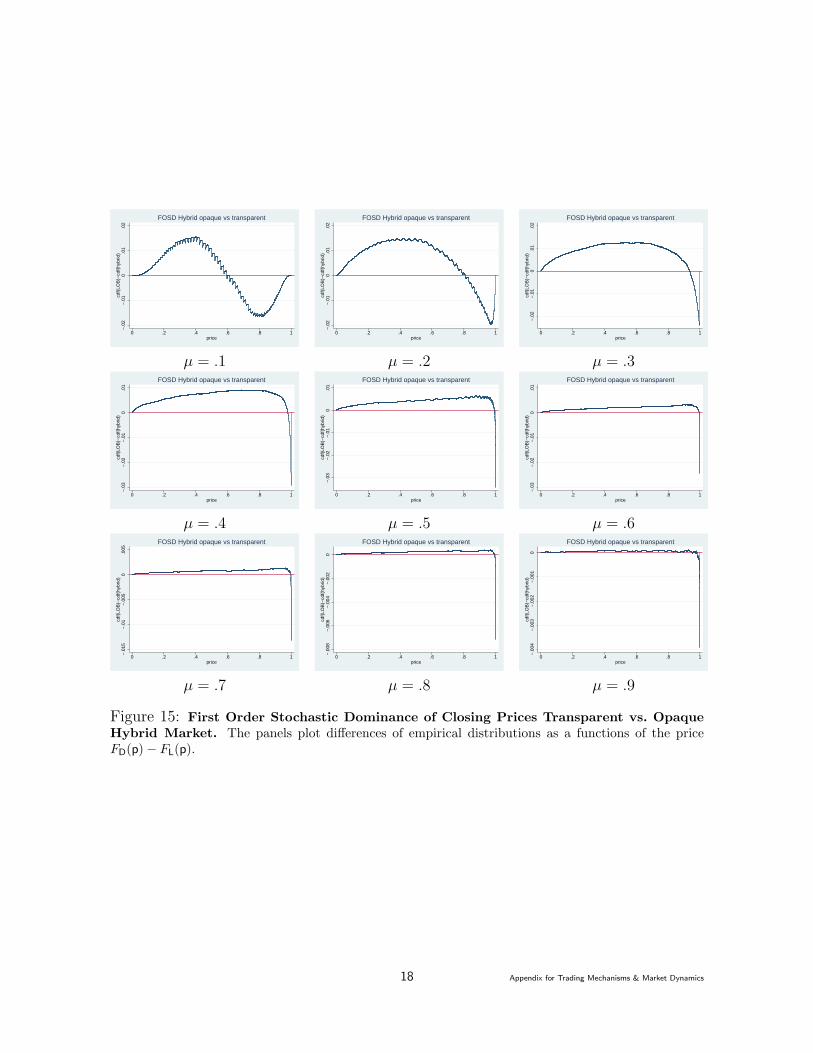
Figure 15: First Order Stochastic Dominance of Closing Prices Transparent vs. Opaque
Hybrid Market. The panels plot differences of empirical distributions as a functions of the priceFD(p) − FL(p).
18 Appendix for Trading Mechanisms & Market Dynamics
010
2030
4050
ccdf
(LO
B)−
ccdf
(hyb
rid)
0 .2 .4 .6 .8 1price
SOSD Hybrid opaque vs transparent
020
4060
80cc
df(L
OB
)−cc
df(h
ybrid
)
0 .2 .4 .6 .8 1price
SOSD Hybrid opaque vs transparent
020
4060
80cc
df(L
OB
)−cc
df(h
ybrid
)
0 .2 .4 .6 .8 1price
SOSD Hybrid opaque vs transparent
µ = .1 µ = .2 µ = .3
020
4060
80cc
df(L
OB
)−cc
df(h
ybrid
)
0 .2 .4 .6 .8 1price
SOSD Hybrid opaque vs transparent
010
2030
40cc
df(L
OB
)−cc
df(h
ybrid
)
0 .2 .4 .6 .8 1price
SOSD Hybrid opaque vs transparent
05
1015
20cc
df(L
OB
)−cc
df(h
ybrid
)
0 .2 .4 .6 .8 1price
SOSD Hybrid opaque vs transparent
µ = .4 µ = .5 µ = .6
02
46
8cc
df(L
OB
)−cc
df(h
ybrid
)
0 .2 .4 .6 .8 1price
SOSD Hybrid opaque vs transparent
0.5
11.
52
ccdf
(LO
B)−
ccdf
(hyb
rid)
0 .2 .4 .6 .8 1price
SOSD Hybrid opaque vs transparent
0.2
.4.6
ccdf
(LO
B)−
ccdf
(hyb
rid)
0 .2 .4 .6 .8 1price
SOSD Hybrid opaque vs transparent
µ = .7 µ = .8 µ = .9
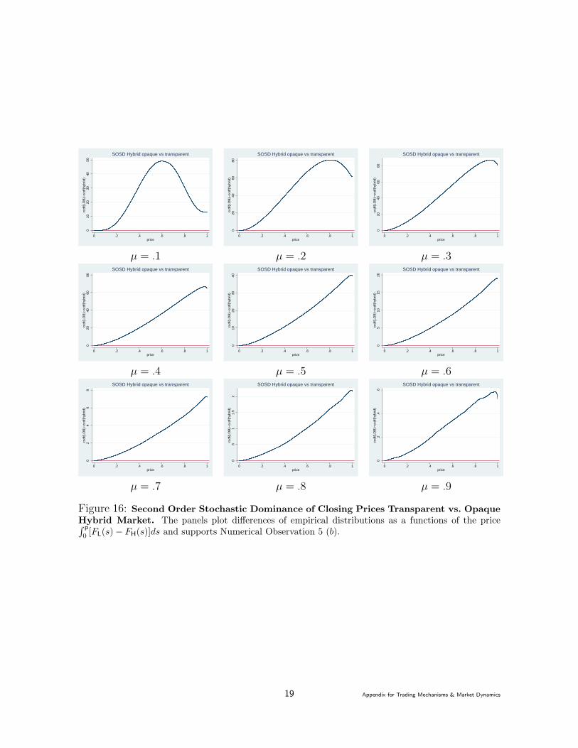
Figure 16: Second Order Stochastic Dominance of Closing Prices Transparent vs. Opaque
Hybrid Market. The panels plot differences of empirical distributions as a functions of the price∫ p
0[FL(s) − FH(s)]ds and supports Numerical Observation 5 (b).
19 Appendix for Trading Mechanisms & Market Dynamics