The ESCRT-III molecules regulate the apical targeting of ...
Structure, Volume 20 Supplemental Information
Solution Structure of the ESCRT-I and -II
Supercomplex: Implications
for Membrane Budding and Scission
Evzen Boura, Bartosz Różycki, Hoi Sung Chung, Dawn Z. Herrick, Bertram Canagarajah, David S. Cafiso, William A. Eaton, Gerhard Hummer, and James H. Hurley Inventory of Supplemental Information
Movie S1. Animated model for sorting, budding, and scission. Associated with
Figure 8.
Fig. S1 SAXS analysis. Associated with Figure 1.
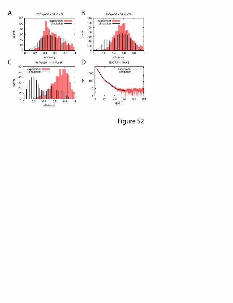
Fig. S2 Simulation of the ESCRT-II complex. Associated with Figure 3.
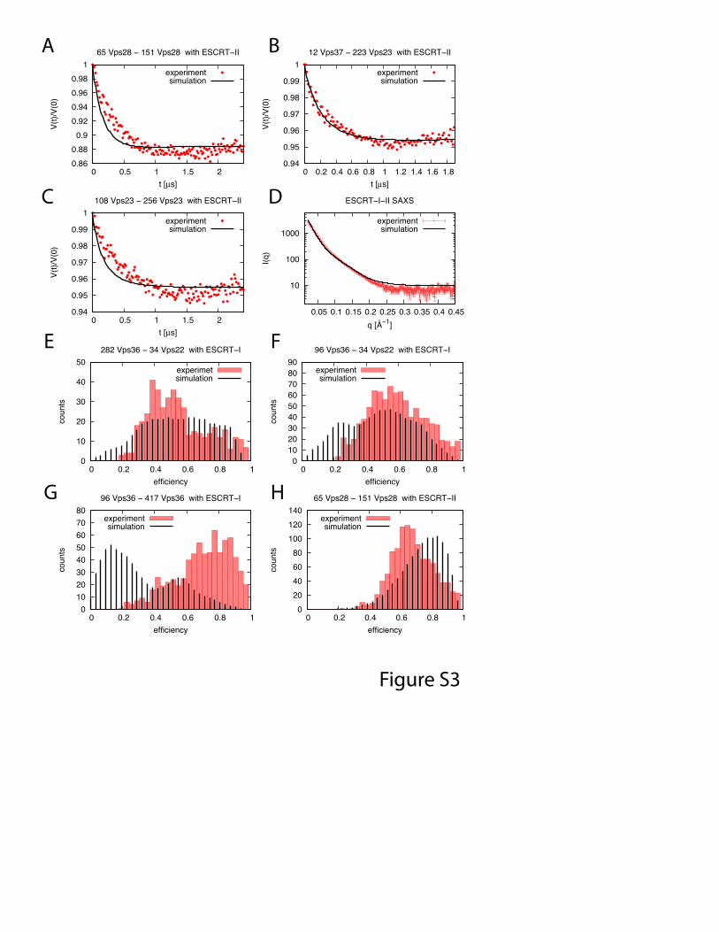
Fig. S3 Simulation of the ESCRT-I-II supercomplex. Associated with Figure 4.
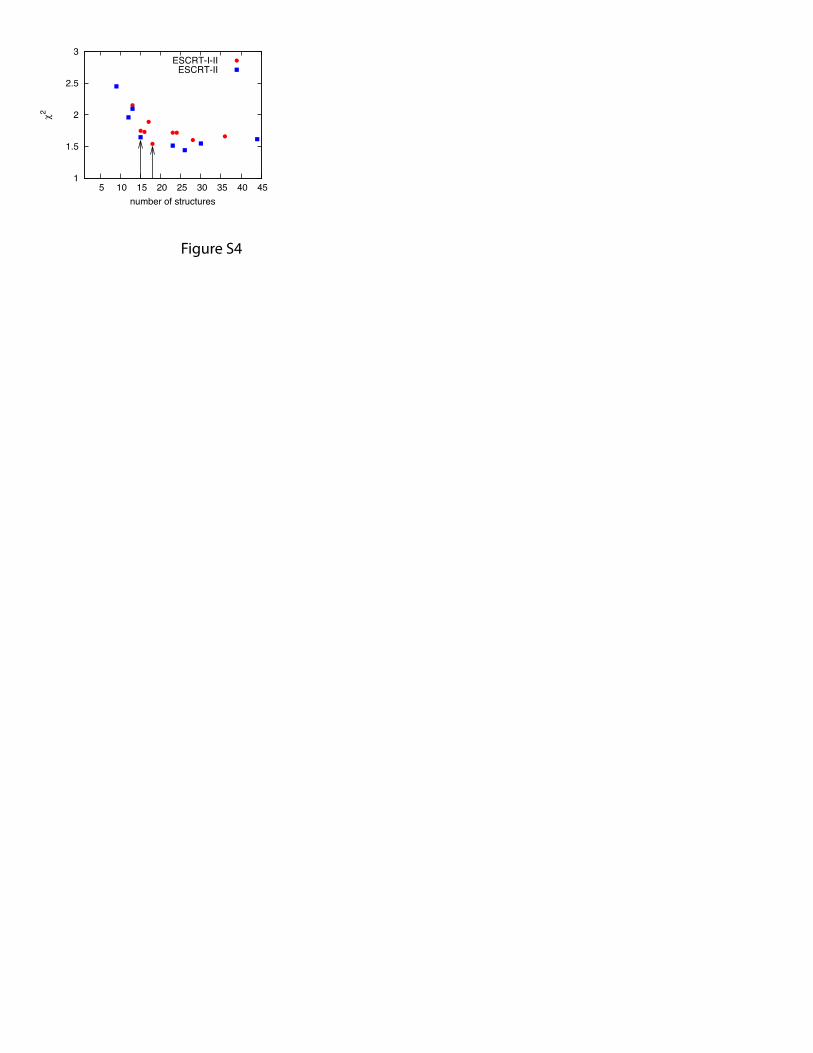
Fig. S4 Dependence of 2 on number of conformations used in fitting. Associated
with Figure 5.
Supplementary Movie and Figure Legends
Movie S1. Animated model for sorting, budding, and scission. See the legend to Fig. 8
for detailed explanations of each event and the data supporting it.
Fig. S1 SAXS analysis. SAXS for ESCRT-I-II at two different concentrations shown
unscaled (A) and scaled (B). Associated with Figure 1.
Fig. S2 Simulation of the ESCRT-II complex. Simulation data before any refinement
(black) are compared to experimental data (red). Panels (A) to (C) show smFRET
efficiency histograms for labels 282 Vps36 - 34 Vps22 (A), 96 Vps36 - 34 Vps22 (B) and
96 Vps36 - 417 Vps36. Panel (D) shows buffer-subtracted SAXS data. Associated with
Figure 3.
Fig. S3 Simulation of the ESCRT-I-II supercomplex. Simulation data before any
refinement (black) are compared to experimental data (red). Panels (A) to (C) show
DEER data for indicated labels. Panel (D) shows buffer-subtracted SAXS data. Panels
(E) to (H) show smFRET efficiency histograms for indicated labels. Associated with
Figure 4.
Fig. S4 Dependence of χ2 on number of conformations used in fitting. The quality of the
fits improves with the addition of more conformations, up to a threshold of 15 for
ESCRT-II alone (blue boxes) or 18 for the ESCRT-I-II supercomplex (red circles).
Associated with Figure 5.
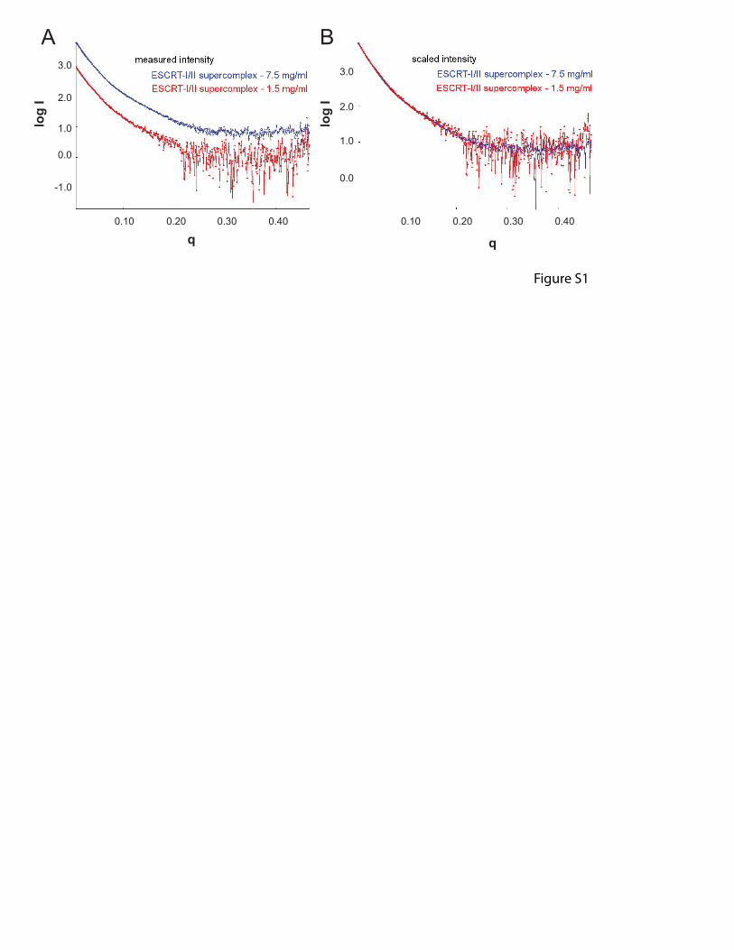
Figure S1
A
-1.0
0.0
1.0
2.0
3.0
log
IB
0.0
1.0
2.0
3.0
log
I
0.10 0.20 0.30 0.40 0.10 0.20 0.30 0.40
q q
0
20
40
60
80
100
120
0 0.2 0.4 0.6 0.8 1
coun
ts
efficiency
282 Vps36 − 34 Vps22
experimentsimulation
0 20 40 60 80
100 120 140
0 0.2 0.4 0.6 0.8 1
coun
ts
efficiency
96 Vps36 − 34 Vps22
experimentsimulation
0
10
20
30
40
50
60
0 0.2 0.4 0.6 0.8 1
coun
ts
efficiency
96 Vps36 − 417 Vps36
experimentsimulation
1
10
100
1000
0 0.1 0.2 0.3 0.4 0.5
I(q)
q [Å−1]
ESCRT−II SAXS
experimentsimulation
Figure S2
D
A B
C
0.94
0.95
0.96
0.97
0.98
0.99
1
0 0.5 1 1.5 2
V(t)/
V(0)
t [µs]
108 Vps23 − 256 Vps23 with ESCRT−II
experimentsimulation
0.94
0.95
0.96
0.97
0.98
0.99
1
0 0.2 0.4 0.6 0.8 1 1.2 1.4 1.6 1.8
V(t)/
V(0)
t [µs]
12 Vps37 − 223 Vps23 with ESCRT−II
experimentsimulation
0.86 0.88
0.9 0.92 0.94 0.96 0.98
1
0 0.5 1 1.5 2
V(t)/
V(0)
t [µs]
65 Vps28 − 151 Vps28 with ESCRT−II
experimentsimulation
10
100
1000
0.05 0.1 0.15 0.2 0.25 0.3 0.35 0.4 0.45
I(q)
q [Å−1]
ESCRT−I−II SAXS
experimentsimulation
0
10
20
30
40
50
0 0.2 0.4 0.6 0.8 1
coun
ts
efficiency
282 Vps36 − 34 Vps22 with ESCRT−I
experimetsimulation
0 10 20 30 40 50 60 70 80 90
0 0.2 0.4 0.6 0.8 1
coun
ts
efficiency
96 Vps36 − 34 Vps22 with ESCRT−I
experimentsimulation
0 10 20 30 40 50 60 70 80
0 0.2 0.4 0.6 0.8 1
coun
ts
efficiency
96 Vps36 − 417 Vps36 with ESCRT−I
experimentsimulation
0 20 40 60 80
100 120 140
0 0.2 0.4 0.6 0.8 1
coun
ts
efficiency
65 Vps28 − 151 Vps28 with ESCRT−II
experimentsimulation
Figure S3
D
A B
C
H
E F
G
1
1.5
2
2.5
3
5 10 15 20 25 30 35 40 45
χ2
number of structures
ESCRT-I-IIESCRT-II
Figure S4