TasNat 1928 Vol2 No4 Pp2-5 Crowther TasNatHistInterestingAspects

Contents
LMER model selection 2
Linear regression models 8
CI for parameter range . . . . . . . . . . . . . . . . . . . . . . . . . . . . . . . . . . . . . . . . . . . 8
Global Extrapolations . . . . . . . . . . . . . . . . . . . . . . . . . . . . . . . . . . . . . . . . . . . 11
Figures 15
Change in carbon per degree year with bootstrap (Figure 1) . . . . . . . . . . . . . . . . . . . . . . 15
Model-data plot for interactive statisitcal model (Figure 2a) . . . . . . . . . . . . . . . . . . . . . . 17
Boot strap slope comparison (Figure 2b) . . . . . . . . . . . . . . . . . . . . . . . . . . . . . . . . . 19
Global carbon vulnerability map (Figure 3a) . . . . . . . . . . . . . . . . . . . . . . . . . . . . . . 23
Effect-time assumptions affects soil carbon losses (Figure 3b) . . . . . . . . . . . . . . . . . . . . . 24
Data summary and basic visualizations 25
Helper functions 34
Bootstrap function . . . . . . . . . . . . . . . . . . . . . . . . . . . . . . . . . . . . . . . . . . . . . 34
Read data . . . . . . . . . . . . . . . . . . . . . . . . . . . . . . . . . . . . . . . . . . . . . . . . . . 34
Construct study means and standard deviations . . . . . . . . . . . . . . . . . . . . . . . . . . . . . 35
Convert R data.frame to netCDF file . . . . . . . . . . . . . . . . . . . . . . . . . . . . . . . . . . . 36
Main analysis script . . . . . . . . . . . . . . . . . . . . . . . . . . . . . . . . . . . . . . . . . . . . 38
Extrapolation code . . . . . . . . . . . . . . . . . . . . . . . . . . . . . . . . . . . . . . . . . . . . . 43
Global carbon loss map code . . . . . . . . . . . . . . . . . . . . . . . . . . . . . . . . . . . . . . . 50
List of Tables
1 Model fits comparing the statistical power gained by of treatment (degree-Years, and degree;addative.treat and addative.dT respectively) vs enviromental variables (MAT, MAP, and pH;addative.enviro) vs all variables include (addative.enviro) to explaining warmed soil carbonstocks. . . . . . . . . . . . . . . . . . . . . . . . . . . . . . . . . . . . . . . . . . . . . . . . . . 7
2 Model fits comparing the statistical power gained by multiplicative vs addative models usingthe controlled soil carbon stocks and degree-years or degrees warmed to explain warmed soilcarbon stocks. The interactive degree-years model (interactive) signficantly better then thealternative models (interactive.dT, addative.treat, and simple) considered. . . . . . . . . . . . 7
WWW.NATURE.COM/NATURE | 1
SUPPLEMENTARY INFORMATIONdoi:10.1038/nature20150
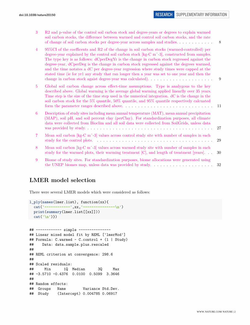
3 R2 and p-value of the control soil carbon stock and degree-years or degrees to explain warmedsoil carbon stocks, the difference between warmed and control soil carbon stocks, and the rateof change of soil carbon stocks per degree-year across samples and studies. . . . . . . . . . . . 8
4 95%CI of the coefficents and R2 of the change in soil carbon stocks (warmed-controlled) perdegree-year explained by the control soil carbon stock [kg-C mˆ-3], constructed from samples.The type key is as follows: dCperDegYr is the change in carbon stock regressed against thedegree-year, dCperDeg is the change in carbon stock regressed against the degrees warmed,and the time notates a dC per degree-year regression where study times were capped at thestated time (ie for yr1 any study that ran longer then a year was set to one year and then thechange in carbon stock agaist degree-year was calculated). . . . . . . . . . . . . . . . . . . . . 9
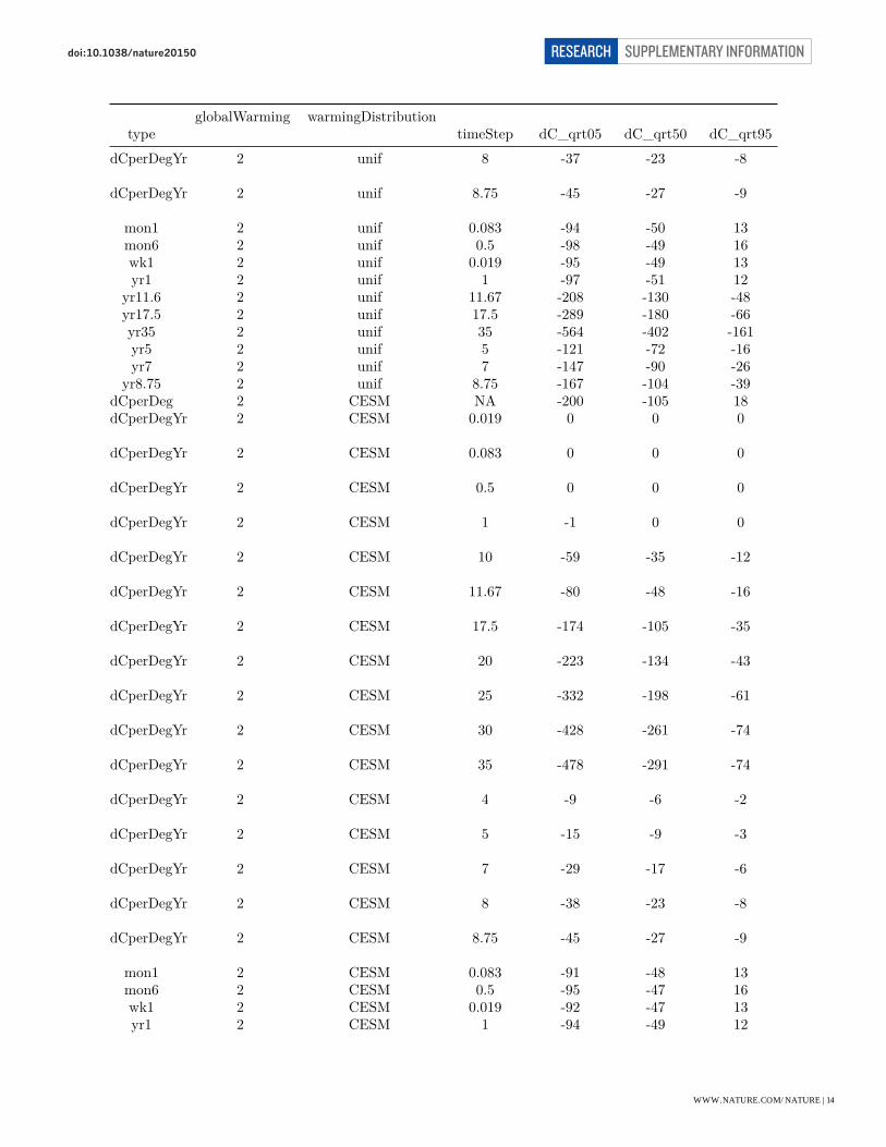
5 Global soil carbon change across effect-time assumptions. Type is analygous to the keydescribed above. Global warming is the average global warming applied linearlly over 35 years.Time step is the size of the time step used in the numerical integration. dC is the change in thesoil carbon stock for the 5% quantile, 50% quantile, and 95% quantile respectively calcuatedform the parameter ranges described above. . . . . . . . . . . . . . . . . . . . . . . . . . . . . 11
6 Description of study sites including mean annual temperature (MAT), mean annual precipitation(MAP), soil pH, and soil percent clay (perClay). For standardization purposes, all climatedata were collected from Bioclim and all soil data were collected from SoilGrids, unless datawas provided by study. . . . . . . . . . . . . . . . . . . . . . . . . . . . . . . . . . . . . . . . . 27
7 Mean soil carbon [kg-C mˆ-3] values across control study site with number of samples in eachstudy for the control plots. . . . . . . . . . . . . . . . . . . . . . . . . . . . . . . . . . . . . . 29
8 Mean soil carbon [kg-C mˆ-3] values across warmed study site with number of samples in eachstudy for the warmed plots, their warming treatment [C], and length of treatment [years]. . . 30
9 Biome of study sites. For standardization purposes, biome allocations were generated usingthe UNEP biomes map, unless data was provided by study. . . . . . . . . . . . . . . . . . . . 32
LMER model selection
There were several LMER models which were considered as follows:
l_ply(names(lmer.list), function(xx){cat('------------',xx,'---------------\n')print(summary(lmer.list[[xx]]))cat('\n')})
## ------------ simple ---------------## Linear mixed model fit by REML ['lmerMod']## Formula: C.warmed ~ C.control + (1 | Study)## Data: data.sample.plus.rescaled#### REML criterion at convergence: 298.6#### Scaled residuals:## Min 1Q Median 3Q Max## -3.5710 -0.4376 0.0100 0.5099 3.3646#### Random effects:## Groups Name Variance Std.Dev.## Study (Intercept) 0.004785 0.06917
WWW.NATURE.COM/NATURE | 2
SUPPLEMENTARY INFORMATIONRESEARCHdoi:10.1038/nature20150

## Residual 0.224720 0.47405## Number of obs: 213, groups: Study, 47#### Fixed effects:## Estimate Std. Error t value## (Intercept) 0.12979 0.04796 2.706## C.control 0.86890 0.03401 25.548#### Correlation of Fixed Effects:## (Intr)## C.control -0.701#### ------------ addative.dT ---------------## Linear mixed model fit by REML ['lmerMod']## Formula: C.warmed ~ C.control + Tdelta + (1 | Study)## Data: data.sample.plus.rescaled#### REML criterion at convergence: 302.4#### Scaled residuals:## Min 1Q Median 3Q Max## -3.5657 -0.4340 0.0158 0.5067 3.3363#### Random effects:## Groups Name Variance Std.Dev.## Study (Intercept) 0.0008106 0.02847## Residual 0.2281379 0.47764## Number of obs: 213, groups: Study, 47#### Fixed effects:## Estimate Std. Error t value## (Intercept) 0.15543 0.05478 2.837## C.control 0.88241 0.03342 26.406## Tdelta -0.03801 0.03348 -1.135#### Correlation of Fixed Effects:## (Intr) C.cntr## C.control -0.519## Tdelta -0.523 -0.146#### ------------ addative.all ---------------## Linear mixed model fit by REML ['lmerMod']## Formula: C.warmed ~ C.control + MAP + MAT + pH + degYr + perClay + (1 |## Study)## Data: data.sample.plus.rescaled#### REML criterion at convergence: 310.9#### Scaled residuals:## Min 1Q Median 3Q Max## -3.3695 -0.5154 0.0043 0.4686 3.5373#### Random effects:## Groups Name Variance Std.Dev.
WWW.NATURE.COM/NATURE | 3
SUPPLEMENTARY INFORMATIONRESEARCHdoi:10.1038/nature20150

## Study (Intercept) 0.004465 0.06682## Residual 0.219005 0.46798## Number of obs: 213, groups: Study, 47#### Fixed effects:## Estimate Std. Error t value## (Intercept) 0.08816 0.07787 1.132## C.control 0.83458 0.03868 21.576## MAP 0.14869 0.06882 2.161## MAT -0.16039 0.06317 -2.539## pH 0.11411 0.05062 2.254## degYr -0.06862 0.03717 -1.846## perClay 0.04239 0.03852 1.100#### Correlation of Fixed Effects:## (Intr) C.cntr MAP MAT pH degYr## C.control -0.384## MAP -0.247 -0.444## MAT -0.004 0.456 -0.801## pH -0.365 -0.261 0.693 -0.545## degYr -0.143 0.040 -0.272 0.140 -0.399## perClay -0.199 0.131 -0.177 -0.074 -0.269 0.063#### ------------ addative.enviro ---------------## Linear mixed model fit by REML ['lmerMod']## Formula: C.warmed ~ C.control + MAP + MAT + pH + perClay + (1 | Study)## Data: data.sample.plus.rescaled#### REML criterion at convergence: 309.4#### Scaled residuals:## Min 1Q Median 3Q Max## -3.3981 -0.4809 0.0177 0.5070 3.5172#### Random effects:## Groups Name Variance Std.Dev.## Study (Intercept) 0.01051 0.1025## Residual 0.21674 0.4656## Number of obs: 213, groups: Study, 47#### Fixed effects:## Estimate Std. Error t value## (Intercept) 0.07561 0.08078 0.936## C.control 0.82323 0.04028 20.438## MAP 0.12463 0.06944 1.795## MAT -0.15238 0.06553 -2.325## pH 0.08068 0.04869 1.657## perClay 0.04554 0.04062 1.121#### Correlation of Fixed Effects:## (Intr) C.cntr MAP MAT pH## C.control -0.374## MAP -0.305 -0.446## MAT 0.019 0.449 -0.798
WWW.NATURE.COM/NATURE | 4
SUPPLEMENTARY INFORMATIONRESEARCHdoi:10.1038/nature20150
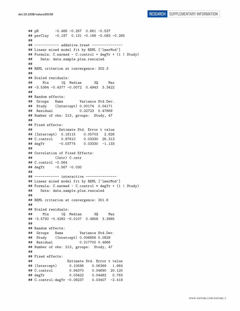
## pH -0.466 -0.267 0.661 -0.537## perClay -0.197 0.131 -0.168 -0.083 -0.265#### ------------ addative.treat ---------------## Linear mixed model fit by REML ['lmerMod']## Formula: C.warmed ~ C.control + degYr + (1 | Study)## Data: data.sample.plus.rescaled#### REML criterion at convergence: 302.3#### Scaled residuals:## Min 1Q Median 3Q Max## -3.5364 -0.4377 -0.0072 0.4943 3.3422#### Random effects:## Groups Name Variance Std.Dev.## Study (Intercept) 0.00174 0.04171## Residual 0.22723 0.47669## Number of obs: 213, groups: Study, 47#### Fixed effects:## Estimate Std. Error t value## (Intercept) 0.16115 0.05703 2.826## C.control 0.87610 0.03330 26.313## degYr -0.03774 0.03330 -1.133#### Correlation of Fixed Effects:## (Intr) C.cntr## C.control -0.564## degYr -0.567 -0.030#### ------------ interactive ---------------## Linear mixed model fit by REML ['lmerMod']## Formula: C.warmed ~ C.control * degYr + (1 | Study)## Data: data.sample.plus.rescaled#### REML criterion at convergence: 301.6#### Scaled residuals:## Min 1Q Median 3Q Max## -3.5792 -0.4282 -0.0107 0.4858 3.3985#### Random effects:## Groups Name Variance Std.Dev.## Study (Intercept) 0.006856 0.0828## Residual 0.217700 0.4666## Number of obs: 213, groups: Study, 47#### Fixed effects:## Estimate Std. Error t value## (Intercept) 0.10596 0.06369 1.664## C.control 0.94370 0.04690 20.120## degYr 0.03422 0.04482 0.763## C.control:degYr -0.08237 0.03407 -2.418
WWW.NATURE.COM/NATURE | 5
SUPPLEMENTARY INFORMATIONRESEARCHdoi:10.1038/nature20150
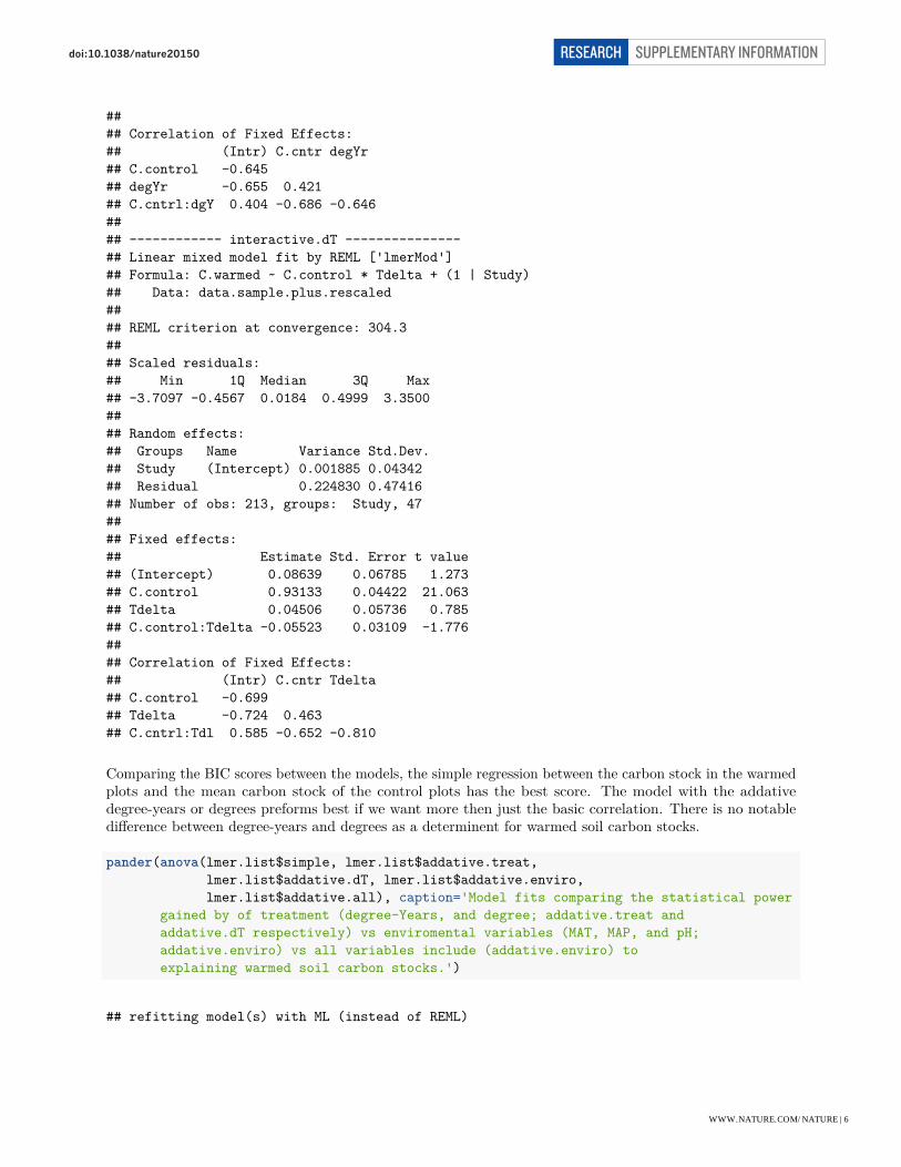
#### Correlation of Fixed Effects:## (Intr) C.cntr degYr## C.control -0.645## degYr -0.655 0.421## C.cntrl:dgY 0.404 -0.686 -0.646#### ------------ interactive.dT ---------------## Linear mixed model fit by REML ['lmerMod']## Formula: C.warmed ~ C.control * Tdelta + (1 | Study)## Data: data.sample.plus.rescaled#### REML criterion at convergence: 304.3#### Scaled residuals:## Min 1Q Median 3Q Max## -3.7097 -0.4567 0.0184 0.4999 3.3500#### Random effects:## Groups Name Variance Std.Dev.## Study (Intercept) 0.001885 0.04342## Residual 0.224830 0.47416## Number of obs: 213, groups: Study, 47#### Fixed effects:## Estimate Std. Error t value## (Intercept) 0.08639 0.06785 1.273## C.control 0.93133 0.04422 21.063## Tdelta 0.04506 0.05736 0.785## C.control:Tdelta -0.05523 0.03109 -1.776#### Correlation of Fixed Effects:## (Intr) C.cntr Tdelta## C.control -0.699## Tdelta -0.724 0.463## C.cntrl:Tdl 0.585 -0.652 -0.810
Comparing the BIC scores between the models, the simple regression between the carbon stock in the warmedplots and the mean carbon stock of the control plots has the best score. The model with the addativedegree-years or degrees preforms best if we want more then just the basic correlation. There is no notabledifference between degree-years and degrees as a determinent for warmed soil carbon stocks.
pander(anova(lmer.list$simple, lmer.list$addative.treat,lmer.list$addative.dT, lmer.list$addative.enviro,lmer.list$addative.all), caption='Model fits comparing the statistical power
gained by of treatment (degree-Years, and degree; addative.treat andaddative.dT respectively) vs enviromental variables (MAT, MAP, and pH;addative.enviro) vs all variables include (addative.enviro) toexplaining warmed soil carbon stocks.')
## refitting model(s) with ML (instead of REML)
WWW.NATURE.COM/NATURE | 6
SUPPLEMENTARY INFORMATIONRESEARCHdoi:10.1038/nature20150

Table 1: Model fits comparing the statistical power gained byof treatment (degree-Years, and degree; addative.treat and adda-tive.dT respectively) vs enviromental variables (MAT, MAP, andpH; addative.enviro) vs all variables include (addative.enviro) toexplaining warmed soil carbon stocks.
Df AIC BIC logLik deviance Chisq Chi DfPr(>Chisq)
lmer.list$simple 4 296.7 310.2 -144.4 288.7 NA NA NA
lmer.list$addative.treat 5 297.4 314.2 -143.7 287.4 1.368 1 0.2422
lmer.list$addative.dT 5 297.4 314.2 -143.7 287.4 0 0 1
lmer.list$addative.enviro 8 297.3 324.2 -140.7 281.3 6.048 3 0.1093
lmer.list$addative.all 9 295.6 325.8 -138.8 277.6 3.785 1 0.0517
The interactive model has both a better AIC and BIC score then even the simple regression. Thus theinterative model is the most parsimonious.
pander(anova(lmer.list$interactive, lmer.list$interactive.dT, lmer.list$addative.treat,lmer.list$simple),
caption='Model fits comparing the statistical power gained by multiplicativevs addative models using the controlled soil carbon stocks and degree-years or degreeswarmed to explain warmed soil carbon stocks. The interactive degree-years model(interactive) signficantly better then the alternative models(interactive.dT, addative.treat, and simple) considered.')
## refitting model(s) with ML (instead of REML)
Table 2: Model fits comparing the statistical power gained by multi-plicative vs addative models using the controlled soil carbon stocksand degree-years or degrees warmed to explain warmed soil carbonstocks. The interactive degree-years model (interactive) signficantlybetter then the alternative models (interactive.dT, addative.treat,and simple) considered.
Df AIC BIC logLik deviance Chisq Chi DfPr(>Chisq)
lmer.list$simple 4 296.7 310.2 -144.4 288.7 NA NA NA
lmer.list$addative.treat 5 297.4 314.2 -143.7 287.4 1.368 1 0.2422
lmer.list$interactive 6 293.7 313.9 -140.8 281.7 5.665 1 0.01731
lmer.list$interactive.dT 6 296.2 316.3 -142.1 284.2 0 0 1
WWW.NATURE.COM/NATURE | 7
SUPPLEMENTARY INFORMATIONRESEARCHdoi:10.1038/nature20150
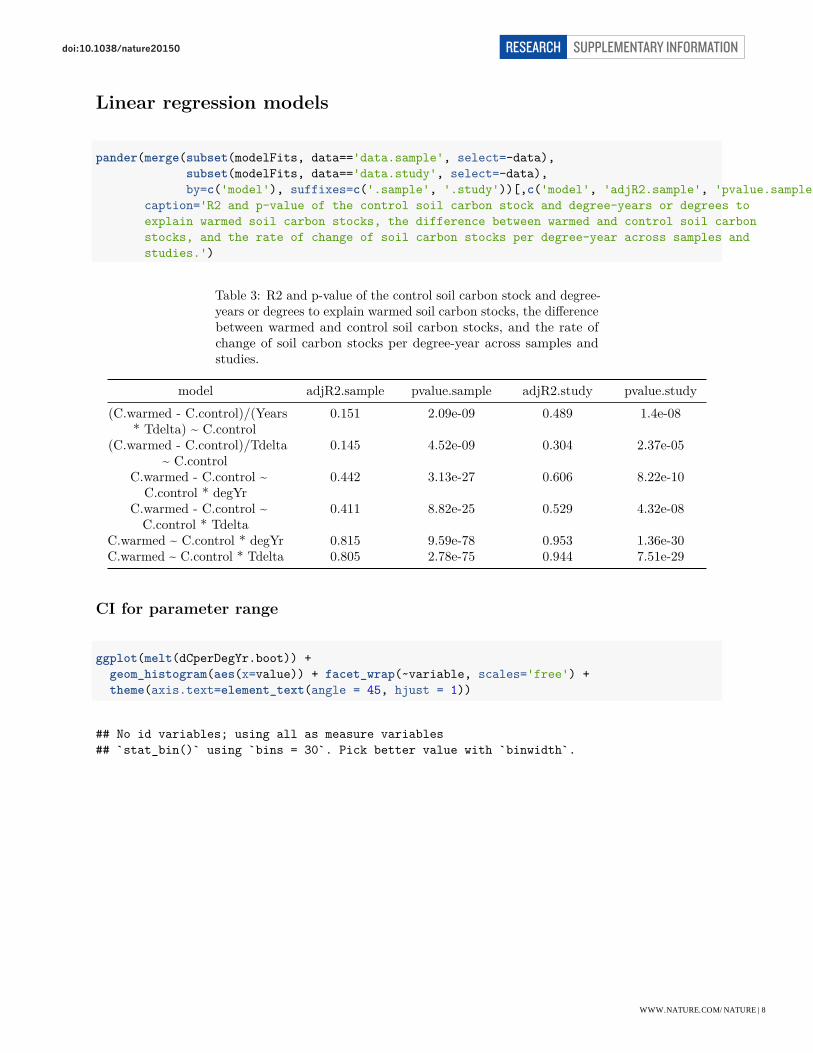
Linear regression models
pander(merge(subset(modelFits, data=='data.sample', select=-data),subset(modelFits, data=='data.study', select=-data),by=c('model'), suffixes=c('.sample', '.study'))[,c('model', 'adjR2.sample', 'pvalue.sample', 'adjR2.study', 'pvalue.study')] ,
caption='R2 and p-value of the control soil carbon stock and degree-years or degrees toexplain warmed soil carbon stocks, the difference between warmed and control soil carbonstocks, and the rate of change of soil carbon stocks per degree-year across samples andstudies.')
Table 3: R2 and p-value of the control soil carbon stock and degree-years or degrees to explain warmed soil carbon stocks, the differencebetween warmed and control soil carbon stocks, and the rate ofchange of soil carbon stocks per degree-year across samples andstudies.
model adjR2.sample pvalue.sample adjR2.study pvalue.study(C.warmed - C.control)/(Years
* Tdelta) ~ C.control0.151 2.09e-09 0.489 1.4e-08
(C.warmed - C.control)/Tdelta~ C.control
0.145 4.52e-09 0.304 2.37e-05
C.warmed - C.control ~C.control * degYr
0.442 3.13e-27 0.606 8.22e-10
C.warmed - C.control ~C.control * Tdelta
0.411 8.82e-25 0.529 4.32e-08
C.warmed ~ C.control * degYr 0.815 9.59e-78 0.953 1.36e-30C.warmed ~ C.control * Tdelta 0.805 2.78e-75 0.944 7.51e-29
CI for parameter range
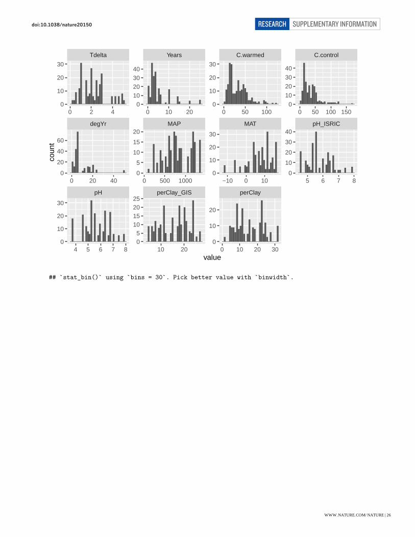
ggplot(melt(dCperDegYr.boot)) +geom_histogram(aes(x=value)) + facet_wrap(~variable, scales='free') +theme(axis.text=element_text(angle = 45, hjust = 1))
## No id variables; using all as measure variables## `stat_bin()` using `bins = 30`. Pick better value with `binwidth`.
WWW.NATURE.COM/NATURE | 8
SUPPLEMENTARY INFORMATIONRESEARCHdoi:10.1038/nature20150

(Intercept) C.control p.value
adj.r.squared r.squard
0
25
50
75
100
0
25
50
75
100
0
250
500
750
0
30
60
90
120
0
50
100
0.6
0.8
1.0
1.2
1.4
−0.0
50
−0.0
45
−0.0
40
−0.0
35
−0.0
30
0e+0
0
1e−0
5
2e−0
5
0.10
0.14
0.18
0.22
0.08
0.12
0.16
0.20
value
coun
t
pander(subset(parRange, type %in% resultsTable$type), caption='95%CI of the coefficents and R2 of the change in soil carbon stocks(warmed-controlled) per degree-year explained by the control soil carbon stock[kg-C m^-3], constructed from samples. The type key is as follows: dCperDegYr is thechange in carbon stock regressed against the degree-year, dCperDeg is the change incarbon stock regressed against the degrees warmed, and the time notates a dC perdegree-year regression where study times were capped at the stated time (ie for yr1 anystudy that ran longer then a year was set to one year and then the change in carbonstock agaist degree-year was calculated). ')
Table 4: 95%CI of the coefficents and R2 of the change in soilcarbon stocks (warmed-controlled) per degree-year explained by thecontrol soil carbon stock [kg-C mˆ-3], constructed from samples.The type key is as follows: dCperDegYr is the change in carbonstock regressed against the degree-year, dCperDeg is the change incarbon stock regressed against the degrees warmed, and the timenotates a dC per degree-year regression where study times werecapped at the stated time (ie for yr1 any study that ran longer thena year was set to one year and then the change in carbon stockagaist degree-year was calculated).
type intercept C p.value adj.r.squared r.squard qrt1 dCperDegYr 0.8866 -0.04358 9.34e-10 0.1089 0.1134 0.05
2 dCperDegYr 1.076 -0.03864 3.083e-08 0.1407 0.145 0.5
WWW.NATURE.COM/NATURE | 9
SUPPLEMENTARY INFORMATIONRESEARCHdoi:10.1038/nature20150

type intercept C p.value adj.r.squared r.squard qrt3 dCperDegYr 1.254 -0.03334 1.188e-06 0.1701 0.1743 0.95
4 dCperDeg 4.001 -0.2091 2.298e-09 0.09723 0.1018 0.05
5 dCperDeg 5.399 -0.1855 9.812e-08 0.1308 0.1352 0.5
6 dCperDeg 6.223 -0.1319 4.448e-06 0.1627 0.1669 0.95
7 wk1 198.6 -10.94 2.241e-09 0.09451 0.09911 0.05
8 wk1 280.4 -9.688 1.216e-07 0.129 0.1334 0.5
9 wk1 323.8 -6.559 6.267e-06 0.1626 0.1668 0.95
10 mon1 46.13 -2.52 1.473e-09 0.09606 0.1006 0.05
11 mon1 64.59 -2.237 1.03e-07 0.1304 0.1348 0.512 mon1 74.9 -1.515 5.263e-06 0.1664 0.1706 0.95
13 mon6 7.253 -0.416 1.98e-09 0.08499 0.08964 0.0514 mon6 10.72 -0.3699 1.025e-07 0.1303 0.1347 0.5
15 mon6 12.34 -0.2427 1.829e-05 0.1633 0.1675 0.95
16 yr1 3.901 -0.2117 1.483e-09 0.09832 0.1029 0.05
17 yr1 5.5 -0.1893 7.171e-08 0.1335 0.1379 0.5
18 yr1 6.268 -0.1288 4.002e-06 0.1659 0.1701 0.95
22 yr5 1.16 -0.0577 2.853e-10 0.1218 0.1262 0.05
23 yr5 1.451 -0.05142 9.718e-09 0.1503 0.1546 0.5
24 yr5 1.688 -0.04257 2.814e-07 0.1799 0.1841 0.95
25 yr7 1.033 -0.05116 1.995e-10 0.1197 0.1241 0.05
26 yr7 1.264 -0.0455 5.731e-09 0.155 0.1593 0.5
27 yr7 1.474 -0.03836 3.57e-07 0.1823 0.1864 0.95
31 yr8.75 0.9666 -0.04752 2.73e-10 0.1166 0.1211 0.05
32 yr8.75 1.169 -0.04227 8.245e-09 0.1518 0.1561 0.5
33 yr8.75 1.348 -0.03643 4.96e-07 0.1803 0.1844 0.95
37 yr11.6 0.9024 -0.04494 5.163e-10 0.1146 0.1191 0.05
38 yr11.6 1.096 -0.03992 1.592e-08 0.1463 0.1506 0.5
WWW.NATURE.COM/NATURE | 10
SUPPLEMENTARY INFORMATIONRESEARCHdoi:10.1038/nature20150

type intercept C p.value adj.r.squared r.squard qrt39 yr11.6 1.281 -0.03461 6.246e-07 0.175 0.1792 0.95
43 yr17.5 0.8823 -0.04337 9.387e-10 0.1086 0.1132 0.05
44 yr17.5 1.067 -0.03851 3.577e-08 0.1394 0.1438 0.5
45 yr17.5 1.246 -0.03345 1.263e-06 0.1701 0.1743 0.95
55 yr35 0.8928 -0.04337 9.072e-10 0.1112 0.1158 0.05
56 yr35 1.071 -0.03878 3.3e-08 0.14 0.1444 0.5
57 yr35 1.243 -0.03366 9.32e-07 0.1702 0.1744 0.95
Global Extrapolations
temp <- subset(resultsTable, globalWarming %in% c(1,2), c('type', 'globalWarming', 'warmingDistribution', 'timeStep', 'dC_qrt05', 'dC_qrt50', 'dC_qrt95') )row.names(temp) <- NULLpander(temp,
caption='Global soil carbon change across effect-time assumptions. Type is analygousto the key described above. Global warming is the average global warming appliedlinearlly over 35 years. Time step is the size of the time step used in the numericalintegration. dC is the change in the soil carbon stock for the 5% quantile, 50% quantile,and 95% quantile respectively calcuated form the parameter ranges described above.',round=c(1,1,1,3,0,0,0))
Table 5: Global soil carbon change across effect-time assumptions.Type is analygous to the key described above. Global warming is theaverage global warming applied linearlly over 35 years. Time step isthe size of the time step used in the numerical integration. dC is thechange in the soil carbon stock for the 5% quantile, 50% quantile,and 95% quantile respectively calcuated form the parameter rangesdescribed above.
typeglobalWarming warmingDistribution
timeStep dC_qrt05 dC_qrt50 dC_qrt95dCperDeg 1 unif NA -103 -55 9dCperDegYr 1 unif 0.019 0 0 0
dCperDegYr 1 unif 0.083 0 0 0
dCperDegYr 1 unif 0.5 0 0 0
dCperDegYr 1 unif 1 0 0 0
dCperDegYr 1 unif 10 -29 -18 -6
dCperDegYr 1 unif 11.67 -40 -24 -8
WWW.NATURE.COM/NATURE | 11
SUPPLEMENTARY INFORMATIONRESEARCHdoi:10.1038/nature20150

typeglobalWarming warmingDistribution
timeStep dC_qrt05 dC_qrt50 dC_qrt95dCperDegYr 1 unif 17.5 -89 -54 -18
dCperDegYr 1 unif 20 -117 -70 -24
dCperDegYr 1 unif 25 -183 -110 -37
dCperDegYr 1 unif 30 -263 -158 -53
dCperDegYr 1 unif 35 -358 -216 -72
dCperDegYr 1 unif 4 -5 -3 -1
dCperDegYr 1 unif 5 -7 -4 -1
dCperDegYr 1 unif 7 -14 -9 -3
dCperDegYr 1 unif 8 -19 -11 -4
dCperDegYr 1 unif 8.75 -22 -13 -5
mon1 1 unif 0.083 -50 -26 7mon6 1 unif 0.5 -51 -26 8wk1 1 unif 0.019 -50 -26 7yr1 1 unif 1 -51 -27 6
yr11.6 1 unif 11.67 -114 -70 -26yr17.5 1 unif 17.5 -161 -99 -36yr35 1 unif 35 -352 -219 -81yr5 1 unif 5 -64 -38 -8yr7 1 unif 7 -79 -48 -14
yr8.75 1 unif 8.75 -90 -56 -20dCperDeg 1 CESM NA -103 -55 9dCperDegYr 1 CESM 0.019 0 0 0
dCperDegYr 1 CESM 0.083 0 0 0
dCperDegYr 1 CESM 0.5 0 0 0
dCperDegYr 1 CESM 1 0 0 0
dCperDegYr 1 CESM 10 -29 -18 -6
dCperDegYr 1 CESM 11.67 -40 -24 -8
dCperDegYr 1 CESM 17.5 -89 -54 -18
dCperDegYr 1 CESM 20 -116 -70 -24
dCperDegYr 1 CESM 25 -177 -107 -35
dCperDegYr 1 CESM 30 -249 -149 -48
WWW.NATURE.COM/NATURE | 12
SUPPLEMENTARY INFORMATIONRESEARCHdoi:10.1038/nature20150

typeglobalWarming warmingDistribution
timeStep dC_qrt05 dC_qrt50 dC_qrt95dCperDegYr 1 CESM 35 -326 -195 -60
dCperDegYr 1 CESM 4 -5 -3 -1
dCperDegYr 1 CESM 5 -7 -4 -2
dCperDegYr 1 CESM 7 -14 -9 -3
dCperDegYr 1 CESM 8 -19 -11 -4
dCperDegYr 1 CESM 8.75 -22 -14 -5
mon1 1 CESM 0.083 -49 -25 7mon6 1 CESM 0.5 -51 -25 8wk1 1 CESM 0.019 -49 -25 7yr1 1 CESM 1 -50 -26 6
yr11.6 1 CESM 11.67 -110 -68 -24yr17.5 1 CESM 17.5 -153 -94 -33yr35 1 CESM 35 -321 -199 -68yr5 1 CESM 5 -63 -37 -8yr7 1 CESM 7 -77 -46 -13
yr8.75 1 CESM 8.75 -88 -54 -19dCperDeg 2 unif NA -206 -109 18dCperDegYr 2 unif 0.019 0 0 0
dCperDegYr 2 unif 0.083 0 0 0
dCperDegYr 2 unif 0.5 0 0 0
dCperDegYr 2 unif 1 -1 0 0
dCperDegYr 2 unif 10 -58 -35 -12
dCperDegYr 2 unif 11.67 -80 -48 -16
dCperDegYr 2 unif 17.5 -179 -108 -36
dCperDegYr 2 unif 20 -234 -141 -47
dCperDegYr 2 unif 25 -365 -220 -74
dCperDegYr 2 unif 30 -524 -317 -106
dCperDegYr 2 unif 35 -569 -397 -144
dCperDegYr 2 unif 4 -9 -6 -2
dCperDegYr 2 unif 5 -15 -9 -3
dCperDegYr 2 unif 7 -29 -17 -6
WWW.NATURE.COM/NATURE | 13
SUPPLEMENTARY INFORMATIONRESEARCHdoi:10.1038/nature20150
typeglobalWarming warmingDistribution
timeStep dC_qrt05 dC_qrt50 dC_qrt95dCperDegYr 2 unif 8 -37 -23 -8
dCperDegYr 2 unif 8.75 -45 -27 -9
mon1 2 unif 0.083 -94 -50 13mon6 2 unif 0.5 -98 -49 16wk1 2 unif 0.019 -95 -49 13yr1 2 unif 1 -97 -51 12
yr11.6 2 unif 11.67 -208 -130 -48yr17.5 2 unif 17.5 -289 -180 -66yr35 2 unif 35 -564 -402 -161yr5 2 unif 5 -121 -72 -16yr7 2 unif 7 -147 -90 -26
yr8.75 2 unif 8.75 -167 -104 -39dCperDeg 2 CESM NA -200 -105 18dCperDegYr 2 CESM 0.019 0 0 0
dCperDegYr 2 CESM 0.083 0 0 0
dCperDegYr 2 CESM 0.5 0 0 0
dCperDegYr 2 CESM 1 -1 0 0
dCperDegYr 2 CESM 10 -59 -35 -12
dCperDegYr 2 CESM 11.67 -80 -48 -16
dCperDegYr 2 CESM 17.5 -174 -105 -35
dCperDegYr 2 CESM 20 -223 -134 -43
dCperDegYr 2 CESM 25 -332 -198 -61
dCperDegYr 2 CESM 30 -428 -261 -74
dCperDegYr 2 CESM 35 -478 -291 -74
dCperDegYr 2 CESM 4 -9 -6 -2
dCperDegYr 2 CESM 5 -15 -9 -3
dCperDegYr 2 CESM 7 -29 -17 -6
dCperDegYr 2 CESM 8 -38 -23 -8
dCperDegYr 2 CESM 8.75 -45 -27 -9
mon1 2 CESM 0.083 -91 -48 13mon6 2 CESM 0.5 -95 -47 16wk1 2 CESM 0.019 -92 -47 13yr1 2 CESM 1 -94 -49 12
WWW.NATURE.COM/NATURE | 14
SUPPLEMENTARY INFORMATIONRESEARCHdoi:10.1038/nature20150

typeglobalWarming warmingDistribution
timeStep dC_qrt05 dC_qrt50 dC_qrt95yr11.6 2 CESM 11.67 -194 -120 -42yr17.5 2 CESM 17.5 -255 -157 -52yr35 2 CESM 35 -472 -297 -88yr5 2 CESM 5 -116 -68 -14yr7 2 CESM 7 -139 -85 -23
yr8.75 2 CESM 8.75 -157 -97 -35
Figures
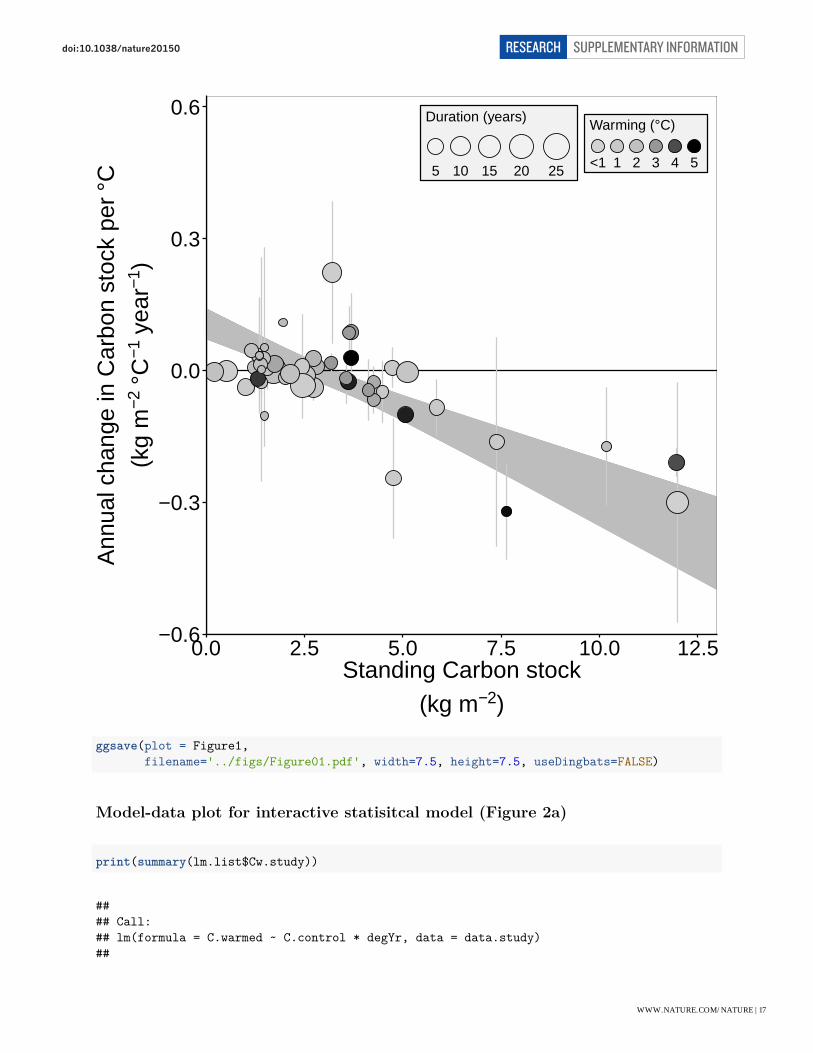
Change in carbon per degree year with bootstrap (Figure 1)
Fig1.theme <- theme(axis.text.x=element_text(size=18,angle=0,colour="black"),axis.text.y=element_text(size=18,angle=0,colour="black"),axis.title=element_text(size=20),legend.text=element_text(size=12),axis.line.x=element_line(color="black"),legend.position = "top",legend.key = element_rect(fill="grey95",size=0,color="grey95"),legend.key.size = unit(0.1,"cm"),legend.title = element_text(size=12,face="bold"),legend.background = element_rect(fill="grey95",color="black"),axis.line = element_line(colour = "black"),panel.grid.major = element_blank(),panel.grid.minor = element_blank(),strip.background = element_rect(colour = "black",size = 0.5),panel.background = element_rect(colour="black", fill="white"),panel.border = element_blank(),axis.ticks = element_line(colour="black"),legend.box = "horizontal",axis.title.y=element_text(vjust=1.9),axis.title.x=element_text(vjust=-0.4))+theme(legend.justification=c(1,1),legend.position=c(1,1))
# set color gradient#ramp <- colorRamp(c("black","darkred","red"))ramp <- colorRamp(c('lightgrey', 'grey', 'black'))use.col.points <- c(rgb( ramp(seq(0, 1, length = 500)), max = 255))
# generate figure 1fieldDepth <- 0.1Figure1 <- ggplot(data.study,aes(x=C.control*fieldDepth, y=dC.perDegYr*fieldDepth)) +
geom_abline(aes(intercept=parBins$intercept*fieldDepth, slope=parBins$slope),colour="grey",data=parBins) +
geom_abline(intercept=0,slope=0,color="black") +geom_errorbar(aes(ymax=(dC.perDegYr + dC.perDegYr.se)*fieldDepth,
ymin=(dC.perDegYr - dC.perDegYr.se)*fieldDepth),width=0,color="grey80",size=0.5) +
WWW.NATURE.COM/NATURE | 15
SUPPLEMENTARY INFORMATIONRESEARCHdoi:10.1038/nature20150
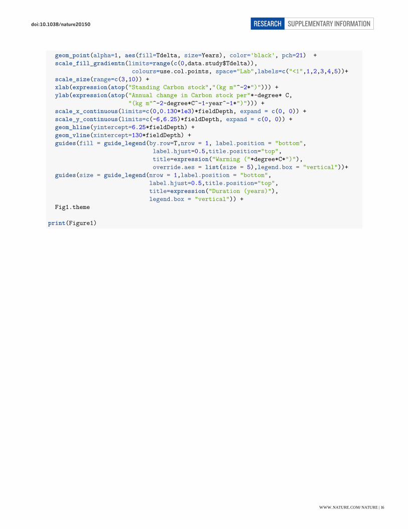
geom_point(alpha=1, aes(fill=Tdelta, size=Years), color='black', pch=21) +scale_fill_gradientn(limits=range(c(0,data.study$Tdelta)),
colours=use.col.points, space="Lab",labels=c("<1",1,2,3,4,5))+scale_size(range=c(3,10)) +xlab(expression(atop("Standing Carbon stock","(kg m"^-2*")"))) +ylab(expression(atop("Annual change in Carbon stock per"*~degree* C,
"(kg m"^-2~degree*C^-1~year^-1*")"))) +scale_x_continuous(limits=c(0,0.130*1e3)*fieldDepth, expand = c(0, 0)) +scale_y_continuous(limits=c(-6,6.25)*fieldDepth, expand = c(0, 0)) +geom_hline(yintercept=6.25*fieldDepth) +geom_vline(xintercept=130*fieldDepth) +guides(fill = guide_legend(by.row=T,nrow = 1, label.position = "bottom",
label.hjust=0.5,title.position="top",title=expression("Warming ("*degree*C*")"),override.aes = list(size = 5),legend.box = "vertical"))+
guides(size = guide_legend(nrow = 1,label.position = "bottom",label.hjust=0.5,title.position="top",title=expression("Duration (years)"),legend.box = "vertical")) +
Fig1.theme
print(Figure1)
WWW.NATURE.COM/NATURE | 16
SUPPLEMENTARY INFORMATIONRESEARCHdoi:10.1038/nature20150
−0.6
−0.3
0.0
0.3
0.6
0.0 2.5 5.0 7.5 10.0 12.5Standing Carbon stock
(kg m−2)
Ann
ual c
hang
e in
Car
bon
stoc
k pe
r °C
(kg
m−2
°C−1
yea
r−1)
Duration (years)
5 10 15 20 25
Warming (°C)
<1 1 2 3 4 5
ggsave(plot = Figure1,filename='../figs/Figure01.pdf', width=7.5, height=7.5, useDingbats=FALSE)
Model-data plot for interactive statisitcal model (Figure 2a)
print(summary(lm.list$Cw.study))
#### Call:## lm(formula = C.warmed ~ C.control * degYr, data = data.study)##
WWW.NATURE.COM/NATURE | 17
SUPPLEMENTARY INFORMATIONRESEARCHdoi:10.1038/nature20150

## Residuals:## Min 1Q Median 3Q Max## -10.3269 -2.1202 -0.5347 0.8649 14.0377#### Coefficients:## Estimate Std. Error t value Pr(>|t|)## (Intercept) 1.61834 1.56580 1.034 0.307## C.control 0.96045 0.03789 25.350 < 2e-16 ***## degYr 0.30065 0.12352 2.434 0.019 *## C.control:degYr -0.01662 0.00321 -5.176 5.11e-06 ***## ---## Signif. codes: 0 '***' 0.001 '**' 0.01 '*' 0.05 '.' 0.1 ' ' 1#### Residual standard error: 4.924 on 45 degrees of freedom## Multiple R-squared: 0.9563, Adjusted R-squared: 0.9534## F-statistic: 328.4 on 3 and 45 DF, p-value: < 2.2e-16
#ramp <- colorRamp(c("white","blue","gold","orange","red"))ramp <- colorRamp(c('white', 'darkgrey'))use.fill <- rgb( ramp(seq(0, 1, length = 255)), max = 255)fig2aTheme <- theme(axis.text.x=element_text(size=18,angle=0,colour="black"),
axis.text.y=element_text(size=18,angle=0,colour="black"),axis.title=element_text(size=20),axis.line = element_line(colour = "black"),panel.grid.major = element_blank(),panel.grid.minor = element_blank(),strip.background = element_rect(colour = "black",size = 0.5),panel.background = element_rect(colour="black", fill="white"),panel.border = element_blank(),axis.ticks = element_line(colour="black"),legend.box = "vertical",legend.justification=c(0.9,1), legend.position=c(0.3,1),legend.key = element_rect(fill="grey95",size=0,color="grey95"),legend.key.size = unit(0.5,"cm"),legend.title = element_text(size=12,face="bold"),legend.background = element_rect(fill="grey95",color="black"))
figure2a <- ggplot(modelData.df,aes(x=rnd.data,y=rnd.model)) +stat_density2d(geom = "raster",aes(fill = ..density..), contour = FALSE,
interpolate = TRUE,n=200,show.legend=T) +geom_point(size=0.15,alpha=0.2,col="grey") +geom_point(data=summaryMD.df,aes(x=data.mean, y=model.mean),
color="black", size=2) +scale_fill_gradientn(colours = use.fill) +geom_abline(intercept=0,slope=1,size=1)+scale_x_log10(limits=c(10,0.12*1e3), expand = c(0, 0),
breaks=c(1:10)*10,labels=c(10,"",30,"",50,"",70,"","",100)) +scale_y_log10(limits=c(10,0.12*1e3), expand = c(0, 0),
breaks=c(1:10)*10,labels=c(10,"",30,"",50,"",70,"","",100)) +xlab(bquote("Observed C stock (kg "*m^-3*")")) +ylab(bquote("Predicted C stock (kg "*m^-3*")")) +guides( fill = guide_colourbar(label.position = "bottom",
label.hjust=0.5,title.position="top",title=expression("Point density"), direction = "horizontal")) +
fig2aTheme
WWW.NATURE.COM/NATURE | 18
SUPPLEMENTARY INFORMATIONRESEARCHdoi:10.1038/nature20150
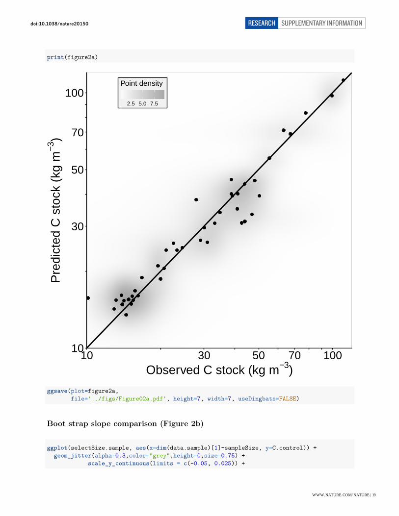
print(figure2a)
10
30
50
70
100
10 30 50 70 100Observed C stock (kg m−3)
Pre
dict
ed C
sto
ck (
kg m
−3)
2.5 5.0 7.5
Point density
ggsave(plot=figure2a,file='../figs/Figure02a.pdf', height=7, width=7, useDingbats=FALSE)
Boot strap slope comparison (Figure 2b)
ggplot(selectSize.sample, aes(x=dim(data.sample)[1]-sampleSize, y=C.control)) +geom_jitter(alpha=0.3,color="grey",height=0,size=0.75) +
scale_y_continuous(limits = c(-0.05, 0.025)) +
WWW.NATURE.COM/NATURE | 19
SUPPLEMENTARY INFORMATIONRESEARCHdoi:10.1038/nature20150
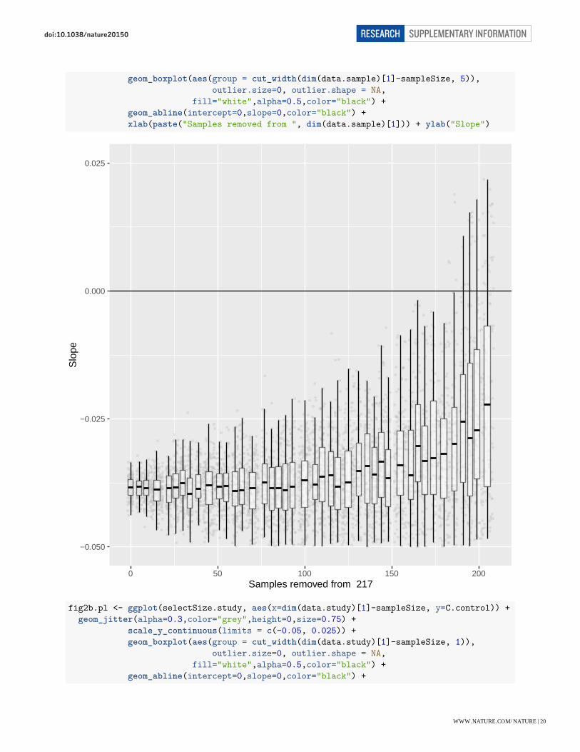
geom_boxplot(aes(group = cut_width(dim(data.sample)[1]-sampleSize, 5)),outlier.size=0, outlier.shape = NA,
fill="white",alpha=0.5,color="black") +geom_abline(intercept=0,slope=0,color="black") +xlab(paste("Samples removed from ", dim(data.sample)[1])) + ylab("Slope")
−0.050
−0.025
0.000
0.025
0 50 100 150 200Samples removed from 217
Slo
pe
fig2b.pl <- ggplot(selectSize.study, aes(x=dim(data.study)[1]-sampleSize, y=C.control)) +geom_jitter(alpha=0.3,color="grey",height=0,size=0.75) +
scale_y_continuous(limits = c(-0.05, 0.025)) +geom_boxplot(aes(group = cut_width(dim(data.study)[1]-sampleSize, 1)),
outlier.size=0, outlier.shape = NA,fill="white",alpha=0.5,color="black") +
geom_abline(intercept=0,slope=0,color="black") +
WWW.NATURE.COM/NATURE | 20
SUPPLEMENTARY INFORMATIONRESEARCHdoi:10.1038/nature20150
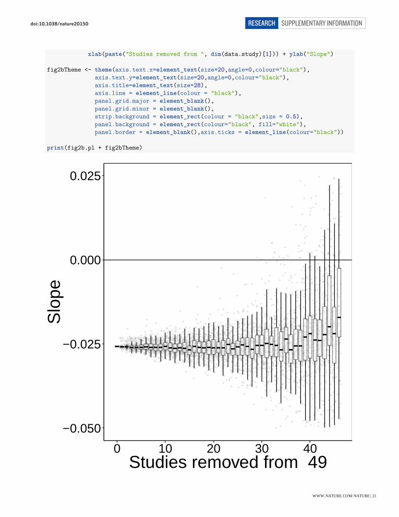
xlab(paste("Studies removed from ", dim(data.study)[1])) + ylab("Slope")
fig2bTheme <- theme(axis.text.x=element_text(size=20,angle=0,colour="black"),axis.text.y=element_text(size=20,angle=0,colour="black"),axis.title=element_text(size=28),axis.line = element_line(colour = "black"),panel.grid.major = element_blank(),panel.grid.minor = element_blank(),strip.background = element_rect(colour = "black",size = 0.5),panel.background = element_rect(colour="black", fill="white"),panel.border = element_blank(),axis.ticks = element_line(colour="black"))
print(fig2b.pl + fig2bTheme)
−0.050
−0.025
0.000
0.025
0 10 20 30 40Studies removed from 49
Slo
pe
WWW.NATURE.COM/NATURE | 21
SUPPLEMENTARY INFORMATIONRESEARCHdoi:10.1038/nature20150

ggsave('../figs/Figure02b.pdf', fig2b.pl + fig2bTheme, width=7, height=7, useDingbats=FALSE)
WWW.NATURE.COM/NATURE | 22
SUPPLEMENTARY INFORMATIONRESEARCHdoi:10.1038/nature20150

Global carbon vulnerability map (Figure 3a)
See Section “Global carbon loss map code”
WWW.NATURE.COM/NATURE | 23
SUPPLEMENTARY INFORMATIONRESEARCHdoi:10.1038/nature20150
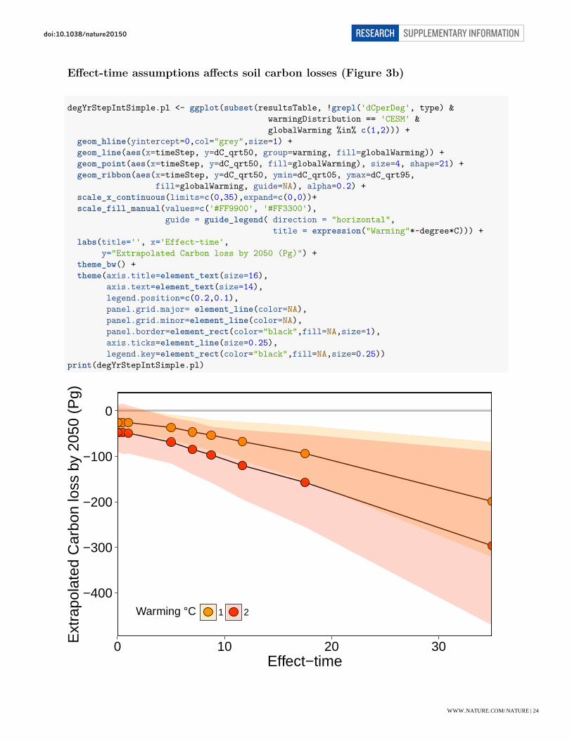
Effect-time assumptions affects soil carbon losses (Figure 3b)
degYrStepIntSimple.pl <- ggplot(subset(resultsTable, !grepl('dCperDeg', type) &warmingDistribution == 'CESM' &globalWarming %in% c(1,2))) +
geom_hline(yintercept=0,col="grey",size=1) +geom_line(aes(x=timeStep, y=dC_qrt50, group=warming, fill=globalWarming)) +geom_point(aes(x=timeStep, y=dC_qrt50, fill=globalWarming), size=4, shape=21) +geom_ribbon(aes(x=timeStep, y=dC_qrt50, ymin=dC_qrt05, ymax=dC_qrt95,
fill=globalWarming, guide=NA), alpha=0.2) +scale_x_continuous(limits=c(0,35),expand=c(0,0))+scale_fill_manual(values=c('#FF9900', '#FF3300'),
guide = guide_legend( direction = "horizontal",title = expression("Warming"*~degree*C))) +
labs(title='', x='Effect-time',y="Extrapolated Carbon loss by 2050 (Pg)") +
theme_bw() +theme(axis.title=element_text(size=16),
axis.text=element_text(size=14),legend.position=c(0.2,0.1),panel.grid.major= element_line(color=NA),panel.grid.minor=element_line(color=NA),panel.border=element_rect(color="black",fill=NA,size=1),axis.ticks=element_line(size=0.25),legend.key=element_rect(color="black",fill=NA,size=0.25))
print(degYrStepIntSimple.pl)
−400
−300
−200
−100
0
0 10 20 30Effect−time
Ext
rapo
late
d C
arbo
n lo
ss b
y 20
50 (
Pg)
Warming °C 1 2
WWW.NATURE.COM/NATURE | 24
SUPPLEMENTARY INFORMATIONRESEARCHdoi:10.1038/nature20150
ggsave(degYrStepIntSimple.pl, filename='../figs/Figure03b.pdf',height=4.5, width=6.5, useDingbats=FALSE)
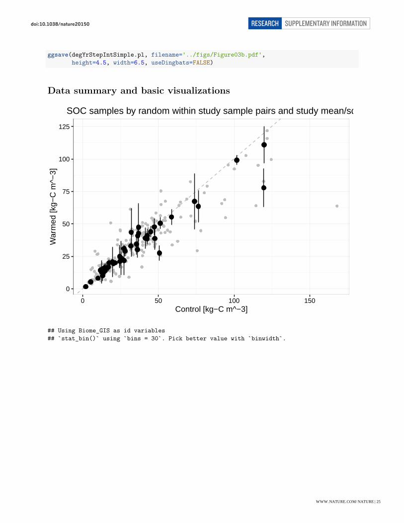
Data summary and basic visualizations
0
25
50
75
100
125
0 50 100 150Control [kg−C m^−3]
War
med
[kg−
C m
^−3]
SOC samples by random within study sample pairs and study mean/sd
## Using Biome_GIS as id variables## `stat_bin()` using `bins = 30`. Pick better value with `binwidth`.
WWW.NATURE.COM/NATURE | 25
SUPPLEMENTARY INFORMATIONRESEARCHdoi:10.1038/nature20150
Tdelta Years C.warmed C.control
degYr MAP MAT pH_ISRIC
pH perClay_GIS perClay
0
10
20
30
010203040
0
10
20
30
0
10
20
30
40
0
20
40
60
0
5
10
15
20
0
10
20
30
0
10
20
30
40
0
10
20
30
05
10152025
0
10
20
0 2 4 0 10 20 0 50 100 0 50 100 150
0 20 40 0 500 1000 −10 0 10 5 6 7 8
4 5 6 7 8 10 20 0 10 20 30value
coun
t
## `stat_bin()` using `bins = 30`. Pick better value with `binwidth`.
WWW.NATURE.COM/NATURE | 26
SUPPLEMENTARY INFORMATIONRESEARCHdoi:10.1038/nature20150

Tdelta Years C.warmed
C.control degYr MAT
MAP pH perClay
0
10
20
30
0
10
20
30
0
5
10
15
20
0
5
10
15
20
0
10
20
30
0
5
10
15
20
0
10
20
0
10
20
30
0
10
20
−1 0 1 2 3 −1 0 1 2 3 −2 0 2
−2 0 2 4 −1 0 1 2 3 −2 −1 0 1 2
−1 0 1 2 3 −1 0 1 2 3 −1 0 1 2 3value
coun
t
Table 6: Description of study sites including mean annual tempera-ture (MAT), mean annual precipitation (MAP), soil pH, and soilpercent clay (perClay). For standardization purposes, all climatedata were collected from Bioclim and all soil data were collectedfrom SoilGrids, unless data was provided by study.
Study Description MAT MAP pH perClayDelta Junction, AK, USA -3.2 298 6.6 12Ford Forest, MI, USA 4.4 824 5.3 8
Ford Forest, MI, USA [precipitation] 4.4 824 5.3 8FRAGILE Experiment, Svalbard,
Norway [grazed]-5.7 226 6 10
FRAGILE Experiment, Svalbard,Norway
-5.7 226 6 10
INCREASE Clocaenog, Wales, UK 7.1 1215 5.2 11Gucheng, Hebei, China 12.7 543 7 17
Soil Warming x Nitrogen AdditionStudy, NH, USA
6.8 1142 4.9 7
Rocky Mountain Biological Laboratory,CO, USA
0.5 519 5.8 14
INCREASE Kiskunsag, Hungary 10.9 536 7.1 1INCREASE Brandbjerg, Demark 8.2 603 5.5 8
Krycklan, Sweden 1 609 4.6 5Jasper Ridge, CA, USA 13.7 635 6.2 18
Jasper Ridge, CA, USA [CO2] 13.7 635 6.2 18Oak Ridge, Tennessee, USA 13.9 1347 5.6 27
Oak Ridge, Tennessee, USA [CO2] 13.9 1347 5.6 27
WWW.NATURE.COM/NATURE | 27
SUPPLEMENTARY INFORMATIONRESEARCHdoi:10.1038/nature20150

Study Description MAT MAP pH perClayOklahoma Tall Grass Prairie, OK, USA
[clipped grass]16.3 906 6.7 8
Oklahoma Tall Grass Prairie, OK, USA 16.3 906 6.7 8Research Station of Songnen Grassland
Ecosystem, China5.2 436 7.9 17
Duke Forest, NC, USA [3 degrees] 14.4 1161 4.9 22Duke Forest, NC, USA [5 degrees] 14.4 1161 4.9 22
Konza Prairie, KS, USA 12 872 6.4 24Whitehall, GA, USA [3 degrees] 16.5 1230 4.6 21Whitehall, GA, USA [5 degrees] 16.5 1230 4.6 21Dry Heath Env. Control, Sweden -0.1 390 5.1 6
Prairie Heating and CO2 Enrichment,WY, USA
7 384 7.4 23
INCREASE Garraf, Spain 15.5 632 6.8 25HOCC-Experiment, Germany 8.9 729 6.3 22HOCC-Experiment, Germany
[precipitation 1]8.9 729 6.3 22
HOCC-Experiment, Germany[precipitation 2]
8.9 729 6.3 22
HOCC-Experiment, Germany[precipitation 3]
8.9 729 6.8 22
HOCC-Experiment, Germany[precipitation 4]
8.9 729 6.8 22
BioCON, MN, USA [elevated C02,ambient N, negative H20]
3.8 761 3.8 11
BioCON, MN, USA [elevated C02,elevated N, negative H20]
3.8 761 3.8 11
BioCON, MN, USA [elevated C02,elevated N, ambient H20]
3.8 761 3.8 11
BioCON, MN, USA [ambient C02,ambient N, ambient H20]
3.8 761 3.8 11
BioCON, MN, USA [ambient C02,elevated N, negative H20]
3.8 761 3.8 11
BioCON, MN, USA [ambient C02,elevated N, ambient H20]
3.8 761 3.8 11
Heating of Prairie Systems 1, OR, USA 11.4 1194 5.3 31Heating of Prairie Systems 1, OR, USA
[precipitation]11.4 1194 5.3 31
Heating of Prairie Systems 2, OR, USA[precipitation]
11.4 1364 5.5 15
Heating of Prairie Systems 3, WA, USA[precipitation]
10.1 1199 5.3 4
Heating of Prairie Systems 2, OR, USA 11.4 1364 5.5 15Heating of Prairie Systems 3, WA, USA 10.1 1199 5.3 4
INCREASE Mols, Denmark 7.4 592 5.3 6Arctic LTER, AK, USA -11.2 237 6 15
Hubbard Brook, NH, USA 5.4 1082 5 9ITEX, Greenland -11.3 112 NA NA
ITEX, Greenland [vegetated] -11.3 112 NA NA
WWW.NATURE.COM/NATURE | 28
SUPPLEMENTARY INFORMATIONRESEARCHdoi:10.1038/nature20150

Table 7: Mean soil carbon [kg-C mˆ-3] values across control studysite with number of samples in each study for the control plots.
Study Description count.control C.control C.sd.controlDelta Junction, AK, USA 5 32.05 NAFord Forest, MI, USA 3 36.19 NA
Ford Forest, MI, USA [precipitation] 3 50.72 NAFRAGILE Experiment, Svalbard,
Norway [grazed]5 58.64 NA
FRAGILE Experiment, Svalbard,Norway
5 73.87 NA
INCREASE Clocaenog, Wales, UK 3 119.9 NAGucheng, Hebei, China 3 101.8 NA
Soil Warming x Nitrogen Addition Study,NH, USA
6 119.6 NA
Rocky Mountain Biological Laboratory,CO, USA
5 17.02 NA
INCREASE Kiskunsag, Hungary 3 5.32 NAINCREASE Brandbjerg, Demark 6 10.13 NA
Krycklan, Sweden 9 44.85 NAJasper Ridge, CA, USA 4 14.04 NA
Jasper Ridge, CA, USA [CO2] 4 15.53 NAOak Ridge, Tennessee, USA 3 27.96 NA
Oak Ridge, Tennessee, USA [CO2] 3 27.32 NAOklahoma Tall Grass Prairie, OK, USA
[clipped grass]6 27.42 NA
Oklahoma Tall Grass Prairie, OK, USA 6 25.27 NAResearch Station of Songnen Grassland
Ecosystem, China6 20.29 NA
Duke Forest, NC, USA [3 degrees] 3 36.89 NADuke Forest, NC, USA [5 degrees] 3 36.89 NA
Konza Prairie, KS, USA 12 47.36 NAWhitehall, GA, USA [3 degrees] 6 12.44 NAWhitehall, GA, USA [5 degrees] 5 13.16 NADry Heath Env. Control, Sweden 6 51.25 NA
Prairie Heating and CO2 Enrichment,WY, USA
5 17.51 NA
INCREASE Garraf, Spain 3 24.42 NAHOCC-Experiment, Germany 4 13.84 NAHOCC-Experiment, Germany
[precipitation 1]4 13.26 NA
HOCC-Experiment, Germany[precipitation 2]
4 11.63 NA
HOCC-Experiment, Germany[precipitation 3]
4 14.55 NA
HOCC-Experiment, Germany[precipitation 4]
4 13.95 NA
BioCON, MN, USA [elevated C02,ambient N, negative H20]
3 13.59 NA
BioCON, MN, USA [elevated C02,elevated N, negative H20]
3 19.6 NA
BioCON, MN, USA [elevated C02,elevated N, ambient H20]
3 14.91 NA
WWW.NATURE.COM/NATURE | 29
SUPPLEMENTARY INFORMATIONRESEARCHdoi:10.1038/nature20150
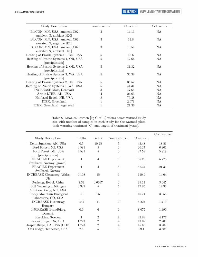
Study Description count.control C.control C.sd.controlBioCON, MN, USA [ambient C02,
ambient N, ambient H20]3 14.13 NA
BioCON, MN, USA [ambient C02,elevated N, negative H20]
3 14.8 NA
BioCON, MN, USA [ambient C02,elevated N, ambient H20]
3 13.54 NA
Heating of Prairie Systems 1, OR, USA 5 42.6 NAHeating of Prairie Systems 1, OR, USA
[precipitation]5 42.66 NA
Heating of Prairie Systems 2, OR, USA[precipitation]
5 31.82 NA
Heating of Prairie Systems 3, WA, USA[precipitation]
5 36.38 NA
Heating of Prairie Systems 2, OR, USA 5 35.57 NAHeating of Prairie Systems 3, WA, USA 5 41.31 NA
INCREASE Mols, Denmark 3 47.64 NAArctic LTER, AK, USA 4 24.63 NA
Hubbard Brook, NH, USA 8 76.38 NAITEX, Greenland 1 2.071 NA
ITEX, Greenland [vegetated] 1 21.36 NA
Table 8: Mean soil carbon [kg-C mˆ-3] values across warmed studysite with number of samples in each study for the warmed plots,their warming treatment [C], and length of treatment [years].
Study Description Tdelta Years count.warmed C.warmedC.sd.warmed
Delta Junction, AK, USA 0.5 10.25 5 43.48 18.56Ford Forest, MI, USA 4.581 5 3 30.27 6.201Ford Forest, MI, USA
[precipitation]4.581 5 3 27.59 5.819
FRAGILE Experiment,Svalbard, Norway [grazed]
1 4 5 55.28 5.773
FRAGILE Experiment,Svalbard, Norway
1 4 5 67.37 21.31
INCREASE Clocaenog, Wales,UK
0.198 15 3 110.9 14.04
Gucheng, Hebei, China 2.34 0.6667 3 99.14 3.645Soil Warming x NitrogenAddition Study, NH, USA
3.989 5 5 77.85 14.91
Rocky Mountain BiologicalLaboratory, CO, USA
2 25 5 16.74 3.056
INCREASE Kiskunsag,Hungary
0.44 14 3 5.227 1.773
INCREASE Brandbjerg,Demark
0.9 6 6 8.075 1.399
Krycklan, Sweden 1 2 9 43.89 4.177Jasper Ridge, CA, USA 1.773 2 4 13.09 2.205
Jasper Ridge, CA, USA [CO2] 1.773 2 4 15.65 3.289Oak Ridge, Tennessee, USA 2.6 5 3 29.1 3.886
WWW.NATURE.COM/NATURE | 30
SUPPLEMENTARY INFORMATIONRESEARCHdoi:10.1038/nature20150
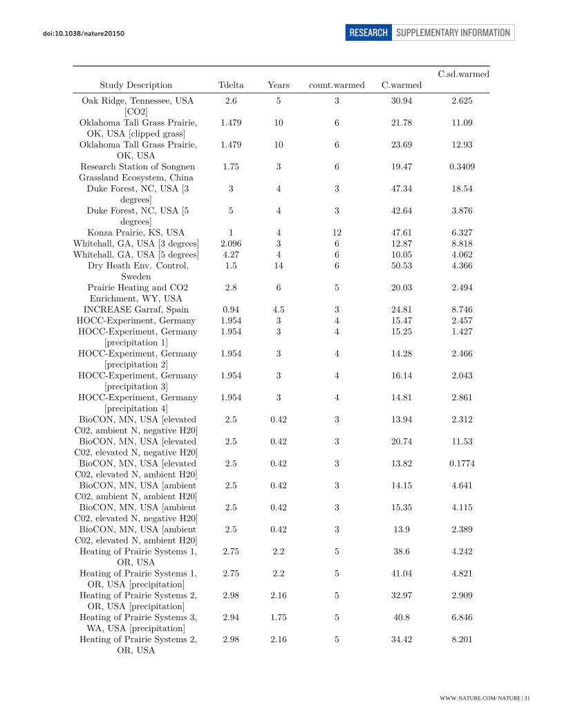
Study Description Tdelta Years count.warmed C.warmedC.sd.warmed
Oak Ridge, Tennessee, USA[CO2]
2.6 5 3 30.94 2.625
Oklahoma Tall Grass Prairie,OK, USA [clipped grass]
1.479 10 6 21.78 11.09
Oklahoma Tall Grass Prairie,OK, USA
1.479 10 6 23.69 12.93
Research Station of SongnenGrassland Ecosystem, China
1.75 3 6 19.47 0.3409
Duke Forest, NC, USA [3degrees]
3 4 3 47.34 18.54
Duke Forest, NC, USA [5degrees]
5 4 3 42.64 3.876
Konza Prairie, KS, USA 1 4 12 47.61 6.327Whitehall, GA, USA [3 degrees] 2.096 3 6 12.87 8.818Whitehall, GA, USA [5 degrees] 4.27 4 6 10.05 4.062
Dry Heath Env. Control,Sweden
1.5 14 6 50.53 4.366
Prairie Heating and CO2Enrichment, WY, USA
2.8 6 5 20.03 2.494
INCREASE Garraf, Spain 0.94 4.5 3 24.81 8.746HOCC-Experiment, Germany 1.954 3 4 15.47 2.457HOCC-Experiment, Germany
[precipitation 1]1.954 3 4 15.25 1.427
HOCC-Experiment, Germany[precipitation 2]
1.954 3 4 14.28 2.466
HOCC-Experiment, Germany[precipitation 3]
1.954 3 4 16.14 2.043
HOCC-Experiment, Germany[precipitation 4]
1.954 3 4 14.81 2.861
BioCON, MN, USA [elevatedC02, ambient N, negative H20]
2.5 0.42 3 13.94 2.312
BioCON, MN, USA [elevatedC02, elevated N, negative H20]
2.5 0.42 3 20.74 11.53
BioCON, MN, USA [elevatedC02, elevated N, ambient H20]
2.5 0.42 3 13.82 0.1774
BioCON, MN, USA [ambientC02, ambient N, ambient H20]
2.5 0.42 3 14.15 4.641
BioCON, MN, USA [ambientC02, elevated N, negative H20]
2.5 0.42 3 15.35 4.115
BioCON, MN, USA [ambientC02, elevated N, ambient H20]
2.5 0.42 3 13.9 2.389
Heating of Prairie Systems 1,OR, USA
2.75 2.2 5 38.6 4.242
Heating of Prairie Systems 1,OR, USA [precipitation]
2.75 2.2 5 41.04 4.821
Heating of Prairie Systems 2,OR, USA [precipitation]
2.98 2.16 5 32.97 2.909
Heating of Prairie Systems 3,WA, USA [precipitation]
2.94 1.75 5 40.8 6.846
Heating of Prairie Systems 2,OR, USA
2.98 2.16 5 34.42 8.201
WWW.NATURE.COM/NATURE | 31
SUPPLEMENTARY INFORMATIONRESEARCHdoi:10.1038/nature20150

Study Description Tdelta Years count.warmed C.warmedC.sd.warmed
Heating of Prairie Systems 3,WA, USA
2.94 1.75 5 39.01 7.942
INCREASE Mols, Denmark 0.9 4 3 38.8 8.516Arctic LTER, AK, USA 0.53 20 4 21.14 3.201
Hubbard Brook, NH, USA 4.83 0.8333 8 63.48 12.36ITEX, Greenland 2 9 1 1.635 NA
ITEX, Greenland [vegetated] 2 9 1 20.02 NA
Table 9: Biome of study sites. For standardization purposes, biomeallocations were generated using the UNEP biomes map, unlessdata was provided by study.
Study Description BiomeDelta Junction, AK, USA Boreal Forests/TaigaFord Forest, MI, USA Temperate Broadleaf and Mixed Forests
Ford Forest, MI, USA [precipitation] Temperate Broadleaf and Mixed ForestsFRAGILE Experiment, Svalbard, Norway
[grazed]Tundra
FRAGILE Experiment, Svalbard, Norway TundraINCREASE Clocaenog, Wales, UK Temperate Grasslands, Savannas and
ShrublandsGucheng, Hebei, China Temperate Grasslands, Savannas and
ShrublandsSoil Warming x Nitrogen Addition Study,
NH, USATemperate Broadleaf and Mixed Forests
Rocky Mountain Biological Laboratory, CO,USA
Temperate Grasslands, Savannas andShrublands
INCREASE Kiskunsag, Hungary Temperate Grasslands, Savannas andShrublands
INCREASE Brandbjerg, Demark Temperate Broadleaf and Mixed ForestsKrycklan, Sweden Boreal Forests/Taiga
Jasper Ridge, CA, USA Temperate Grasslands, Savannas andShrublands
Jasper Ridge, CA, USA [CO2] Temperate Grasslands, Savannas andShrublands
Oak Ridge, Tennessee, USA Temperate Broadleaf and Mixed ForestsOak Ridge, Tennessee, USA [CO2] Temperate Broadleaf and Mixed Forests
Oklahoma Tall Grass Prairie, OK, USA[clipped grass]
Temperate Grasslands, Savannas andShrublands
Oklahoma Tall Grass Prairie, OK, USA Temperate Grasslands, Savannas andShrublands
Research Station of Songnen GrasslandEcosystem, China
Temperate Grasslands, Savannas andShrublands
Duke Forest, NC, USA [3 degrees] Temperate Broadleaf and Mixed ForestsDuke Forest, NC, USA [5 degrees] Temperate Broadleaf and Mixed Forests
Konza Prairie, KS, USA Temperate Grasslands, Savannas andShrublands
Whitehall, GA, USA [3 degrees] Temperate Broadleaf and Mixed ForestsWhitehall, GA, USA [5 degrees] Temperate Broadleaf and Mixed ForestsDry Heath Env. Control, Sweden Tundra
WWW.NATURE.COM/NATURE | 32
SUPPLEMENTARY INFORMATIONRESEARCHdoi:10.1038/nature20150
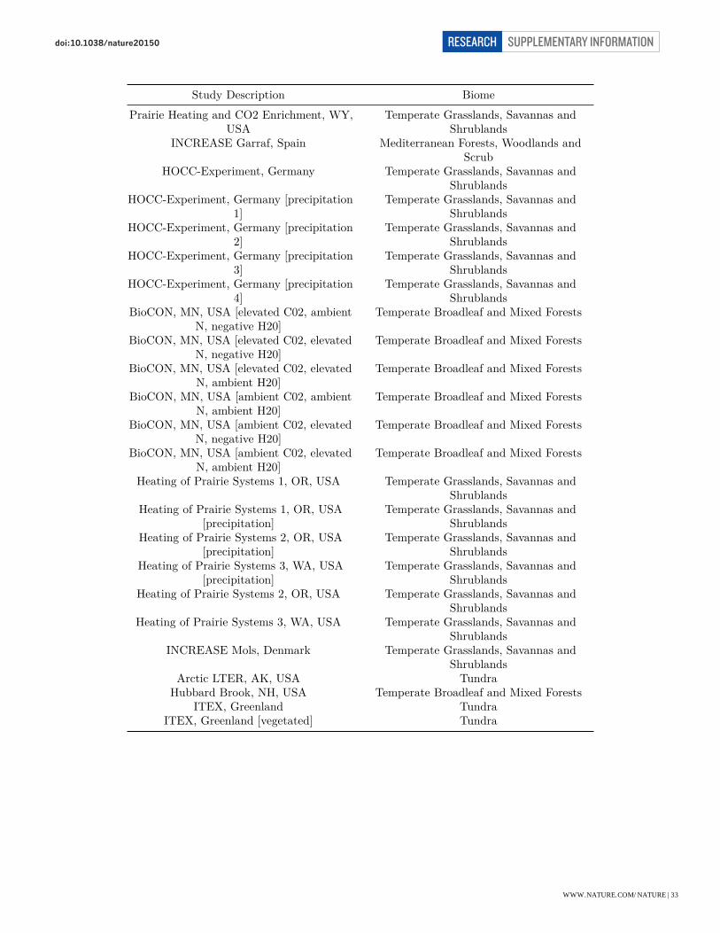
Study Description BiomePrairie Heating and CO2 Enrichment, WY,
USATemperate Grasslands, Savannas and
ShrublandsINCREASE Garraf, Spain Mediterranean Forests, Woodlands and
ScrubHOCC-Experiment, Germany Temperate Grasslands, Savannas and
ShrublandsHOCC-Experiment, Germany [precipitation
1]Temperate Grasslands, Savannas and
ShrublandsHOCC-Experiment, Germany [precipitation
2]Temperate Grasslands, Savannas and
ShrublandsHOCC-Experiment, Germany [precipitation
3]Temperate Grasslands, Savannas and
ShrublandsHOCC-Experiment, Germany [precipitation
4]Temperate Grasslands, Savannas and
ShrublandsBioCON, MN, USA [elevated C02, ambient
N, negative H20]Temperate Broadleaf and Mixed Forests
BioCON, MN, USA [elevated C02, elevatedN, negative H20]
Temperate Broadleaf and Mixed Forests
BioCON, MN, USA [elevated C02, elevatedN, ambient H20]
Temperate Broadleaf and Mixed Forests
BioCON, MN, USA [ambient C02, ambientN, ambient H20]
Temperate Broadleaf and Mixed Forests
BioCON, MN, USA [ambient C02, elevatedN, negative H20]
Temperate Broadleaf and Mixed Forests
BioCON, MN, USA [ambient C02, elevatedN, ambient H20]
Temperate Broadleaf and Mixed Forests
Heating of Prairie Systems 1, OR, USA Temperate Grasslands, Savannas andShrublands
Heating of Prairie Systems 1, OR, USA[precipitation]
Temperate Grasslands, Savannas andShrublands
Heating of Prairie Systems 2, OR, USA[precipitation]
Temperate Grasslands, Savannas andShrublands
Heating of Prairie Systems 3, WA, USA[precipitation]
Temperate Grasslands, Savannas andShrublands
Heating of Prairie Systems 2, OR, USA Temperate Grasslands, Savannas andShrublands
Heating of Prairie Systems 3, WA, USA Temperate Grasslands, Savannas andShrublands
INCREASE Mols, Denmark Temperate Grasslands, Savannas andShrublands
Arctic LTER, AK, USA TundraHubbard Brook, NH, USA Temperate Broadleaf and Mixed Forests
ITEX, Greenland TundraITEX, Greenland [vegetated] Tundra
WWW.NATURE.COM/NATURE | 33
SUPPLEMENTARY INFORMATIONRESEARCHdoi:10.1038/nature20150

Helper functions
Bootstrap function
print(bootStrap.fn)
## function (data, myFormula, nRuns, sampleSize, lm.weights = NULL,## shuffleFn = NULL, numCoef, verbose = FALSE)## {## sampleIndex <- matrix(NA, nrow = nRuns, ncol = sampleSize)## lmStats <- matrix(NA, nrow = nRuns, ncol = numCoef + 3)## for (ii in 1:nRuns) {## if (verbose)## cat(ii, "\n")## if (!is.null(shuffleFn))## data <- shuffleFn(data)## if (verbose)## print(head(data))## sampleIndex[ii, ] <- sample(1:(dim(data)[1]), size = sampleSize)## temp.lm <- lm(myFormula, data[sampleIndex[ii, ], ])## fstatArr <- summary(temp.lm)$fstatistic## if (verbose)## print(summary(temp.lm))## lmStats[ii, ] <- c(temp.lm$coefficients, pf(fstatArr[1],## fstatArr[2], fstatArr[3], lower.tail = FALSE), adj.r.squared = summary(temp.lm)$adj.r.squared,## r.squared = summary(temp.lm)$r.squared)## }## lmStats <- as.data.frame(lmStats)## names(lmStats) <- c(names(temp.lm$coefficients), "p.value",## "adj.r.squared", "r.squard")## if (verbose)## cat("\n")## if (verbose)## print(lmStats)## return(lmStats)## }
Read data
print(readSamples)
## function (filename = "../data/Soil Data Compiled_January 26.xlsx",## useMeanBD = TRUE, readControlMeans = FALSE)## {## data <- read.xlsx2(filename, sheetIndex = 1, colIndex = c(1,## 7, 9, 10, 11, 12))## names(data) <- c("Study", "Treatment", "Tdelta", "Years",## "perC", "bulk_density")## data$Tdelta <- round(data$Tdelta, 3)
WWW.NATURE.COM/NATURE | 34
SUPPLEMENTARY INFORMATIONRESEARCHdoi:10.1038/nature20150
## data$perC <- round(data$perC, 3)## data$bulk_density <- round(data$bulk_density, 3)## if (useMeanBD) {## study.bd <- ddply(data[, c("Study", "bulk_density")],## .(Study), summarize, bulk_density.sd = sd(bulk_density),## bulk_density = mean(bulk_density))## data$bulk_density.sd <- NULL## data$bulk_density <- NULL## data <- merge(study.bd, data)## }## data$C <- data$perC/100 * data$bulk_density## data.sample <- ddply(data, c("Study", "Tdelta", "Years"),## function(xx) {## warmed <- xx$C[xx$Treatment == "W"]## control <- xx$C[xx$Treatment == "C"]## if (readControlMeans) {## return(data.frame(C.warmed = warmed, C.control = mean(control)))## }## else {## mismatch <- length(warmed) - length(control)## if (mismatch > 0) {## control <- c(control, rep(NA, mismatch))## }## else {## warmed <- c(warmed, rep(NA, abs(mismatch)))## }## return(data.frame(C.warmed = warmed, C.control = sample(control)))## }## })## data.sample$degYr <- data.sample$Years * data.sample$Tdelta## return(data.sample)## }
Construct study means and standard deviations
print(readStudyMeans)
## function (filename = "../data/Soil Data Compiled_January 26.xlsx",## includeBD.sd = FALSE, includeControl.sd = FALSE)## {## data <- read.xlsx2(filename, sheetIndex = 1, colIndex = c(1,## 7, 9, 10, 11, 12))## names(data) <- c("Study", "Treatment", "Tdelta", "Years",## "perC", "bulk_density")## data$Tdelta <- round(as.numeric(data$Tdelta), 3)## data$perC <- as.numeric(data$perC)## data$bulk_density <- as.numeric(data$bulk_density)## data.study <- ddply(data, .(Study, Tdelta, Years, Treatment),## summarize, bulk_density.sd = sd(bulk_density), bulk_density = mean(bulk_density),## perC.sd = sd(perC), perC = mean(perC), count = length(Treatment))## if (includeBD.sd) {## data.study$C.sd <- sqrt(data.study$perC/100^2 * data.study$bulk_density.sd^2 +
WWW.NATURE.COM/NATURE | 35
SUPPLEMENTARY INFORMATIONRESEARCHdoi:10.1038/nature20150

## data.study$perC.sd/100^2 * data.study$bulk_density^2)## }## else {## study.bd <- ddply(data[, c("Study", "bulk_density")],## .(Study), summarize, bulk_density = mean(bulk_density))## data.study$bulk_density.sd <- NULL## data.study$bulk_density <- NULL## data.study <- merge(study.bd, data.study)## data.study$C.sd <- sqrt((data.study$perC.sd/100 * data.study$bulk_density)^2)## }## data.study$C <- data.study$perC/100 * data.study$bulk_density## data.study <- merge(subset(data.study, Treatment == "W",## select = -Treatment), subset(data.study, Treatment ==## "C", select = -Treatment), by = c("Study", "Years", "Tdelta"),## suffixes = c(".warmed", ".control"))## if (!includeControl.sd)## data.study$C.sd.control <- 0## data.study$degYr <- data.study$Years * data.study$Tdelta## data.study$dC <- data.study$C.warmed - data.study$C.control## data.study$dC.sd <- sqrt(data.study$C.sd.warmed^2 + data.study$C.sd.control^2)## data.study$dC.perDegYr <- data.study$dC/data.study$degYr## data.study$dC.perDegYr.sd <- data.study$dC.sd/data.study$degYr## if (!includeControl.sd)## data.study$C.sd.control <- NA## data.study$C.se.control <- data.study$C.sd.control/data.study$count.control## data.study$C.se.warmed <- data.study$C.sd.warmed/data.study$count.warmed## data.study$dC.perDegYr.se <- data.study$dC.perDegYr.sd/sqrt(rowMeans(data.study[,## c("count.warmed", "count.control")]))## return(data.study)## }
Convert R data.frame to netCDF file
cat(readLines('../R/Crowther_dSOC_35yr_makeNC.R'), sep = '\n')
## # Crowther_dSOC_35yr_makeNC.r## # Will Wieder## # July 2016## # converts .csv to .nc file## # data reordered go give increasing lat & lon values#### library(ncdf)## library(reshape2)## library(raster)## library(rgdal)#### #dir <- getwd() #"/Users/wwieder/Desktop/Working_files/Crowther_warming/KTB_results/"## #setwd(dir)## file <- "../R/Crowther_dSOC_35yr_makeNC.R"## fin <- "../data/Crowther_dSOC_35yr.csv"## Data <- read.csv(fin)## names(Data)
WWW.NATURE.COM/NATURE | 36
SUPPLEMENTARY INFORMATIONRESEARCHdoi:10.1038/nature20150

#### minLAT <- min(Data$lat)## maxLAT <- max(Data$lat)## minLON <- min(Data$lon)## maxLON <- max(Data$lon)#### attach(Data)## names(Data)#### #set up depth, lat, lon coordinates## nLAT <- length(as.numeric(levels(as.factor(lat))))## nLON <- length(as.numeric(levels(as.factor(lon))))#### #LAT <- seq(minLAT,maxLAT,(90 - 89.05759))## latDATA <- read.csv('../data/LAT.csv') # some rounding errors, read in CSV of LAT from CLM## LAT <- latDATA$LAT## LON <- seq(minLON,maxLON,(360/nLON))## nOBS <- length(Data$dC.single)## dims <- c(nLAT, nLON)#### #something wrong w/ how lat values ordered in .csv file## #rewrite lat so values have a regular step (as I thing they should...)## lat2 <- rep(NA, length(lat))## start <- 1## for (i in 1:nLAT) {## end <- start + nLON-1## lat2[start:end] <- LAT[i]## start <- end + 1## }## #-------------------------------------------------------------## # Define Variables## #-------------------------------------------------------------#### VARS <- c('SOC','landArea','dC.single','dC.multi')## nVARS <- length(VARS)## # close VARS loop## gridSOC <- rasterFromXYZ(data.frame(Data$lon,lat2,Data$SOC), digits=2)## gridSOC <- t(flip(gridSOC, direction='y') )#### gridArea <- rasterFromXYZ(data.frame(Data$lon,lat2,Data$landArea), digits=2)## gridArea <- t(flip(gridArea, direction='y') )#### gridSingle <- rasterFromXYZ(data.frame(Data$lon,lat2,Data$dC.single), digits=2)## gridSingle <- t(flip(gridSingle, direction='y') )#### gridMulti <- rasterFromXYZ(data.frame(Data$lon,lat2,Data$dC.multi), digits=2)## gridMulti <- t(flip(gridMulti, direction='y') )#### #-------------------------------------------------------------## #---------------write out .nc file----------------------------## #-------------------------------------------------------------## # define the netcdf coordinate variables (name, units, type)## lat <- dim.def.ncdf("lat","degrees_north", as.double(LAT), create_dimvar=TRUE)## lon <- dim.def.ncdf("lon","degrees_east", as.double(LON), create_dimvar=TRUE)
WWW.NATURE.COM/NATURE | 37
SUPPLEMENTARY INFORMATIONRESEARCHdoi:10.1038/nature20150

## mv <- -9999. # missing value to use## LATIXY <- var.def.ncdf("LATIXY", "degrees N", list(lat), mv,## longname="latitude", prec="double")## LONGXY <- var.def.ncdf("LONGXY", "degrees E", list(lon), mv,## longname="longitude", prec="double")## SOC_i <- var.def.ncdf("SOC_i", units="kg C/m2", list(lon,lat), mv,## longname="Soil C", prec="double")## area <- var.def.ncdf("Area", units="m2", list(lon,lat), mv,## longname="grid_area", prec="double")## dC_Single <- var.def.ncdf("dC_Single", units="kg C/m2", list(lon,lat), mv,## longname="Single Step", prec="double")## dC_Multi <- var.def.ncdf("dC_Multi", units="kg C/m2", list(lon,lat), mv,## longname="Multi Step", prec="double")#### fname <- '../data/Crowther_dSOC_35y.nc'## ncnew <- create.ncdf( fname, list(LATIXY, LONGXY, SOC_i, area, dC_Single, dC_Multi) )#### # Write some values to this variable on disk.## put.var.ncdf( ncnew, LATIXY, LAT)## put.var.ncdf( ncnew, LONGXY, LON)## put.var.ncdf( ncnew, SOC_i, as.array(gridSOC))## put.var.ncdf( ncnew, area, as.array(gridArea))## put.var.ncdf( ncnew, dC_Single,as.array(gridSingle))## put.var.ncdf( ncnew, dC_Multi ,as.array(gridMulti))#### att.put.ncdf( ncnew, 0, "created_on",date() ,prec=NA,verbose=FALSE,definemode=FALSE )## att.put.ncdf( ncnew, 0, "created_by","Will Wieder",prec=NA,verbose=FALSE,definemode=FALSE )## att.put.ncdf( ncnew, 0, "created_from",fin ,prec=NA,verbose=FALSE,definemode=FALSE )## att.put.ncdf( ncnew, 0, "created_with",file ,prec=NA,verbose=FALSE,definemode=FALSE )#### close.ncdf(ncnew)#### print('-------Wrote out .nc files-----------')## print(ncnew)
Main analysis script
sessionInfo()
R version 3.2.2 (2015-08-14)Platform: x86_64-apple-darwin13.4.0 (64-bit)Running under: OS X 10.10.5 (Yosemite)
locale:[1] en_US.UTF-8/en_US.UTF-8/en_US.UTF-8/C/en_US.UTF-8/en_US.UTF-8
attached base packages:[1] stats graphics grDevices utils datasets methods base
other attached packages:[1] ncdf4_1.15 xlsx_0.5.7 xlsxjars_0.6.1 rJava_0.9-7[5] deSolve_1.12 lme4_1.1-10 Matrix_1.2-3 MASS_7.3-45
WWW.NATURE.COM/NATURE | 38
SUPPLEMENTARY INFORMATIONRESEARCHdoi:10.1038/nature20150
[9] reshape2_1.4.1 pander_0.6.0 plyr_1.8.3 ggplot2_2.0.0
loaded via a namespace (and not attached):[1] Rcpp_0.12.2 knitr_1.11 magrittr_1.5 splines_3.2.2[5] munsell_0.4.2 colorspace_1.2-6 lattice_0.20-33 minqa_1.2.4[9] stringr_1.0.0 tools_3.2.2 grid_3.2.2 gtable_0.1.2
[13] nlme_3.1-122 htmltools_0.2.6 yaml_2.1.13 digest_0.6.8[17] nloptr_1.0.4 formatR_1.2.1 evaluate_0.8 rmarkdown_0.8.1[21] labeling_0.3 stringi_1.0-1 scales_0.3.0
cat(readLines('../R/CrowtherFieldWarmingScript.R'), sep = '\n')
library(ggplot2) #make pretty plotslibrary(plyr) #deal with data frames nicelylibrary(pander) #format tablespanderOptions('table.split.table', Inf) #do not let pander split tables because bad numberinglibrary(reshape2) #deal with data frames nicelylibrary(MASS) #model selectionlibrary(lme4) #random vs fixed effects modellibrary(deSolve) #solve odelibrary(xlsx) #read in excel files
source('../R/bootStrap.fn.R')source('../R/readSamples.R')source('../R/readStudyMeans.R')
verbose <- FALSE
##Helper functionsshuffle.sample <- function(data){
idCol <- setdiff(names(data), c('C.warmed', 'C.control'))return(ddply(data, idCol, summarize,
C.warmed=sample(C.warmed, size=length(Study)),C.control=sample(C.control, size=length(Study))))
}
pullPvalue <- function(temp.lm){fstatArr <- summary(temp.lm)$fstatisticreturn(pf(fstatArr[1], fstatArr[2], fstatArr[3], lower.tail = FALSE))
}
##Read in datastudyMeta <- read.xlsx2('../data/Soil Data Compiled_September 6, 2016.xlsx',
sheetIndex=2, colIndex=c(1, 9, 10, 11, 12, 13, 14, 17, 18),stringsAsFactors=FALSE)
names(studyMeta) <- c('Study', 'MAP', 'MAT', 'Biome_GIS', 'Biome', 'pH_ISRIC', 'pH', 'perClay_GIS', 'perClay')studyMeta$pH <- as.numeric(as.character(studyMeta$pH))studyMeta$perClay <- as.numeric(as.character(studyMeta$perClay))
studyMeta <- studyMeta[studyMeta$Study != '',]
##Replace missing data with data productscat('Replacing ', sum(grepl('^NA$', studyMeta$Biome)), 'of ', dim(studyMeta)[1],' missing biomes with data product.\n')studyMeta$Biome[grepl('^NA$', studyMeta$Biome)] <- studyMeta$Biome_GIS[grepl('^NA$', studyMeta$Biome)]
WWW.NATURE.COM/NATURE | 39
SUPPLEMENTARY INFORMATIONRESEARCHdoi:10.1038/nature20150
cat('Replacing ', sum(is.na(studyMeta$pH)), 'of ', dim(studyMeta)[1],' site missing pH values with data product.\n')studyMeta$pH[is.na(studyMeta$pH)] <- studyMeta$pH_ISRIC[is.na(studyMeta$pH)]
cat('Replacing ', sum(is.na(studyMeta$perClay)), 'of ', dim(studyMeta)[1],' site missing percent clay values with data product.\n')studyMeta$perClay[is.na(studyMeta$perClay)] <- studyMeta$perClay_GIS[is.na(studyMeta$perClay)]
#read study namesstudyNames <- read.xlsx2('../data/Soil Data Compiled_September 6, 2016.xlsx',
sheetIndex=7)names(studyNames) <- c('Study', 'Study Description')data.sample <- readSamples(filename='../data/Soil Data Compiled_September 6, 2016.xlsx')data.study <- readStudyMeans(filename='../data/Soil Data Compiled_September 6, 2016.xlsx')
if(!identical( setdiff(studyMeta$Study, data.sample$Study),setdiff(data.sample$Study, studyMeta$Study)) |
!identical(setdiff(studyMeta$Study, studyNames$Study),setdiff(studyNames$Study, studyMeta$Study))){
stop('study names do not match')}
##Convert from g cm^-3 to kg m^-3data.sample[, c('C.warmed', 'C.control')] <- data.sample[, c('C.warmed', 'C.control')] * 1e3data.study[, c('bulk_density.warmed', 'C.sd.warmed', 'C.warmed', 'bulk_density.control',
'C.sd.control', 'C.control', 'dC', 'dC.sd', 'dC.perDegYr', 'dC.perDegYr.sd','C.se.control', 'C.se.warmed', 'dC.perDegYr.se')] <-
data.study[,c('bulk_density.warmed', 'C.sd.warmed', 'C.warmed', 'bulk_density.control',
'C.sd.control', 'C.control', 'dC', 'dC.sd', 'dC.perDegYr', 'dC.perDegYr.sd','C.se.control', 'C.se.warmed', 'dC.perDegYr.se')] * 1e3
##Rescale data#There is clear skew in the histograms of the years, degree-years, and carbon stocks.#We log-transformed these variables to normalize the distribution for statistical purposes.
data.sample.plus <- merge(data.sample, studyMeta[,c('Study', 'MAT', 'MAP', 'pH', 'perClay')],by='Study', all=TRUE)
data.sample.plus$degYr <- data.sample.plus$Years*data.sample.plus$TdeltafullRows <- apply(subset(data.sample.plus, select=-Study), c(1),
function(xx){all(is.finite(xx))})
if(verbose) print(sprintf('Throwing out %d samples (rows) because of missing values somewhere.',sum(!fullRows)))
data.sample.plus <- data.sample.plus[fullRows,]ggplot(melt(subset(data.sample.plus, select=-Study))) +
geom_histogram(aes(x=value)) + facet_wrap(~variable, scale='free')cor(subset(data.sample.plus, select=-Study))
data.sample.plus.rescaled <- data.sample.plus
data.sample.plus.rescaled$degYr <- log(data.sample.plus.rescaled$degYr)data.sample.plus.rescaled$Years <- log(data.sample.plus$Years)
WWW.NATURE.COM/NATURE | 40
SUPPLEMENTARY INFORMATIONRESEARCHdoi:10.1038/nature20150

data.sample.plus.rescaled$C.control <- log(data.sample.plus$C.control)data.sample.plus.rescaled$C.warmed <- log(data.sample.plus$C.warmed)
data.sample.plus.rescaled[,-1] <- as.data.frame(apply(data.sample.plus.rescaled[, -1], c(2), function(xx){
return((xx-mean(xx, na.rm=TRUE))/sd(xx, na.rm=TRUE)+1)}))
##Construct LMERlmer.list <- list(simple = lmer(C.warmed ~ C.control + (1|Study),
data=data.sample.plus.rescaled),addative.dT = lmer(C.warmed~C.control+Tdelta + (1|Study),
data=data.sample.plus.rescaled),addative.all = lmer(C.warmed~C.control+MAP+MAT+pH+degYr + perClay + (1|Study),
data=data.sample.plus.rescaled),addative.enviro = lmer(C.warmed~C.control+MAP+MAT+pH + perClay+ (1|Study),
data=data.sample.plus.rescaled),addative.treat = lmer(C.warmed~C.control+degYr + (1|Study),
data=data.sample.plus.rescaled),interactive = lmer(C.warmed~C.control*degYr+ (1|Study),
data=data.sample.plus.rescaled),interactive.dT = lmer(C.warmed~C.control*Tdelta+ (1|Study),
data=data.sample.plus.rescaled))
##Construct LMlm.list <- list(Cw.sample = lm(C.warmed ~ C.control * degYr, data.sample),
Cw.sample.dT = lm(C.warmed ~ C.control * Tdelta, data.sample),dC.sample = lm(C.warmed - C.control ~ C.control * degYr, data.sample),dC.dT.sample = lm(C.warmed - C.control ~ C.control * Tdelta, data.sample),dCperDegYr.sample = lm((C.warmed-C.control)/(Years*Tdelta) ~ C.control,
data.sample),dCperDeg.sample = lm((C.warmed-C.control)/Tdelta ~ C.control,
data.sample),Cw.study = lm(C.warmed ~ C.control * degYr, data.study),Cw.study.dT = lm(C.warmed ~ C.control * Tdelta, data.study),dC.study = lm(C.warmed - C.control ~ C.control * degYr, data.study),dC.dT.study = lm(C.warmed - C.control ~ C.control * Tdelta, data.study),dCperDegYr.study = lm((C.warmed-C.control)/(Years*Tdelta) ~ C.control,
data.study),dCperDeg.study = lm((C.warmed-C.control)/Tdelta ~ C.control,
data.study))
modelFits <- ldply(lm.list,function(xx){
data.frame(model=as.character(xx$call)[2],data=as.character(xx$call)[3],adjR2 = sprintf('%0.3f', summary(xx)$adj.r.squared),pvalue=sprintf('%0.3g', pullPvalue(xx)))
})
##Sample model vs data distributionsinteractive.model <- function(pars=summary(lm.list$Cw.study)$coefficients,
C.control, C.sd.control, degYr){
WWW.NATURE.COM/NATURE | 41
SUPPLEMENTARY INFORMATIONRESEARCHdoi:10.1038/nature20150
C_degYr.par <- rnorm(1, mean=pars['C.control:degYr', 'Estimate'],sd=pars['C.control:degYr', 'Std. Error'])
C.par <- rnorm(1, mean=pars['C.control', 'Estimate'], sd=pars['C.control', 'Std. Error'])degYr.par <- rnorm(1, mean=pars['degYr', 'Estimate'], sd=pars['degYr', 'Std. Error'])inter.par <- rnorm(1, mean=pars['(Intercept)', 'Estimate'],
sd=pars['(Intercept)', 'Std. Error'])model <- inter.par+ C.par*C.control + degYr.par*degYr + C_degYr.par*C.control*degYr
return(model)}
modelData.df <- data.frame()for(ii in 1:1000){
modelData.df <- rbind(modelData.df,data.frame(index = 1:length(data.study$C.warmed),
rnd.data=rnorm(n=length(data.study$C.warmed),mean=data.study$C.warmed,sd=data.study$C.sd.warmed),
rnd.model =interactive.model(C.control=data.study$C.control,
C.sd.control=data.study$C.sd.control,degYr=data.study$degYr)))
}
summaryMD.df <- ddply(modelData.df, 'index', summarize,data.mean=mean(rnd.data), data.sd=sd(rnd.data),model.mean=mean(rnd.model), model.sd=sd(rnd.model))
##bootstrap slopeselectSize.sample <- adply(floor(seq(10, dim(data.sample)[1], length=50)), c(1),
function(xx){ans <- bootStrap.fn(
myFormula=(C.warmed-C.control)/(Years*Tdelta) ~ C.control,data=data.sample, nRuns=100, sampleSize=xx, numCoef=2,shuffleFn=shuffle.sample)
ans$sampleSize <- xxreturn(ans)
})
selectSize.study <- adply(3:(dim(data.study)[1]), c(1),function(xx){
ans <- bootStrap.fn(myFormula=(C.warmed-C.control)/(Years*Tdelta) ~ C.control,data=data.study, nRuns=100, sampleSize=xx, numCoef=2)
ans$sampleSize <- xxreturn(ans)
})
##Pull CI for parameters from subset samplesdCperDeg.boot <- bootStrap.fn(
myFormula=(C.warmed-C.control)/Tdelta ~ C.control,data=data.sample, nRuns=1e3, sampleSize=200, numCoef=2, shuffleFn=shuffle.sample)
WWW.NATURE.COM/NATURE | 42
SUPPLEMENTARY INFORMATIONRESEARCHdoi:10.1038/nature20150
dCperDegYr.boot <- bootStrap.fn(myFormula=(C.warmed-C.control)/(Years*Tdelta) ~ C.control,data=data.sample, nRuns=1e3, sampleSize=200, numCoef=2, shuffleFn=shuffle.sample)
dCperDegYr.mod.boot <- llply(list(wk1=1/52, mon1 = 1/12, mon6 = 6/12, yr1 = 1,yr4 = 4, yr5 = 5, yr7 = 7, yr8 = 8,yr8.75= 8.75, yr10 = 10, yr11.6=35/3,yr15 = 15,yr17.5=17.5, yr20 = 20, yr25 = 25, yr30 = 30, yr35 = 35),
function(xx){data.sample$Years.mod <- data.sample$Yearsdata.sample$Years.mod[data.sample$Years.mod > xx] <- xxans <- bootStrap.fn(
myFormula = (C.warmed-C.control)/(Years.mod*Tdelta) ~ C.control,data=data.sample, nRuns=1e3, sampleSize=200,numCoef=2, shuffleFn=shuffle.sample, verbose=FALSE)
return(ans)})
parKDE <- kde2d(dCperDegYr.boot$C.control, dCperDegYr.boot$`(Intercept)`, n=100)parBins <- melt(parKDE$z)parBins <- subset(parBins, value > max(value)*0.01)parBins$slope <- parKDE$x[parBins$Var1]parBins$intercept <- parKDE$y[parBins$Var2]parBins$alpha <- parBins$value/max(parBins$value)
parRange <- ldply(c(list(dCperDegYr = dCperDegYr.boot,dCperDeg = dCperDeg.boot),dCperDegYr.mod.boot), function(xx){ans <- as.data.frame(apply(xx, c(2),
quantile, c(0.05, 0.5, 0.95)))ans$qrt <- c(0.05, 0.5, 0.95)return(ans)})
names(parRange)[1:3] <- c('type','intercept', 'C')save(file='../data/parCIforLM.RData', parRange)
Extrapolation code
cat(readLines('../R/globalExtrapolations.R'), sep='\n')
###Set uplibrary(ncdf4)library(ggplot2)library(plyr)verbose <- FALSEdataDir <- '../data/'readIn.tsl <- TRUE
WWW.NATURE.COM/NATURE | 43
SUPPLEMENTARY INFORMATIONRESEARCHdoi:10.1038/nature20150
################################Read in mapsinputs.ls <- list(soilGrid=list(filename='SoilGrids_0.9x1.25.nc',
varName='OCSTHA_M',units='tonnes ha^-1', #convertion factor 1/10 for kg m^-2depthWeight=c(1, 1, 0, 0, 0, 0)),
#mid points c(2.5 10.0 22.5 45.0 80.0 150.0) cm#implies 5cm, 10cm, 15cm, 30cm, 60cm, 60cm layer lengths#take top 15cm
HWSD=list(filename='surfdata_0.9x1.25_simyr2000_c120906_HWSD_soil.nc',varName='DOM_SOC', #dominatent mapping unit;#alt area weighted AWT_SOCunits='kg C m^-2',depthWeight=c(1, 0)), #0-30 cm, 30-70 cm soil layers
landfrac=list(filename='sftlf_fx_CESM1-BGC_historical_r0i0p0.nc',varName='sftlf',units='percent'),
gridArea=list(filename='areacella_fx_CESM1-BGC_historical_r0i0p0.nc',varName='areacella',units='m2'))
maps.ls <- lapply(inputs.ls, function(args){ncin <- nc_open(sprintf('%s%s', dataDir, args$filename))if(verbose) print(ncin)lon <- ncvar_get(ncin, 'lon') #longitudelat <- ncvar_get(ncin, 'lat') #longitudeans <- ncvar_get(ncin, args$varName)nc_close(ncin)
if(!is.null(args$depthWeight)){ans <- apply(ans, c(1,2), function(xx){sum(args$depthWeight*xx)})
}
dimnames(ans) <- list(lon=lon, lat=lat)ans <- as.data.frame.table(ans, stringsAsFactors=FALSE, responseName='value')ans <- as.data.frame(lapply(ans, as.numeric))
return(ans)})
maps.ls$landArea <- merge(maps.ls$gridArea, maps.ls$landfrac,by=c('lon', 'lat'), suffixes=c('.area', '.perc'))
maps.ls$landArea$value <- maps.ls$landArea$value.area*maps.ls$landArea$value.perc/100
if(readIn.tsl){#CESM1-BGC Soil Temperature##Pre-processing in cdo##$cdo yearmean tsl_Lmon_CESM1-BGC_rcp85_r1i1p1_200601-204912.nc## tsl_yrmean_CESM1-BGC_rcp85_r1i1p1_200601-204912.nc##$cdo sellevidx,1,2,3,4 tsl_yrmean_CESM1-BGC_rcp85_r1i1p1_200601-204912.nc temp.nc##$cdo vertmean temp.nc tsl_yrShortMean_CESM1-BGC_rcp85_r1i1p1_200601-204912.nc
ncin <- nc_open(sprintf('%stsl_yrShortMean_CESM1-BGC_rcp85_r1i1p1_200601-204912.nc',
WWW.NATURE.COM/NATURE | 44
SUPPLEMENTARY INFORMATIONRESEARCHdoi:10.1038/nature20150
dataDir))if(verbose) print(ncin)tsl <- ncvar_get(ncin, 'tsl') #units Klon <- ncvar_get(ncin, 'lon') #longitudelat <- ncvar_get(ncin, 'lat') #longitudetime <- ncvar_get(ncin, 'time') #days since 2005-1-1 0:0:0nc_close(ncin)
dimnames(tsl) <- list(lon=lon, lat=lat, yr=(time/365) + 2005)tsl <- as.data.frame.table(tsl, stringsAsFactors=FALSE, responseName='value')tsl <- as.data.frame(lapply(tsl, as.numeric))
##Make the latitudes aggree, off by 1e-6tsl$lat <- round(tsl$lat, 2)maps.ls <- lapply(maps.ls, function(xx){xx$lat <- round(xx$lat, 2); return(xx)})
##Trim tsl to only cover 2015-2049tsl <- subset(tsl, yr >= 2015 & yr <=2049)tsl.start <- ddply(subset(tsl, yr >= min(yr) & yr < (min(yr)+10)), .(lon, lat),
summarize, value=mean(value))tsl.end <- ddply(subset(tsl, yr > max(yr)-10 & yr <= max(yr)), .(lon, lat),
summarize, value=mean(value))tsl.change <- merge(tsl.start, tsl.end, by=c('lon', 'lat'), suffixes=c('.inital', '.final'))
if(verbose){print(ggplot(tsl.change) + geom_raster(aes(x=lon, y=lat, fill=value.final-value.inital)) +
labs(title='CESM-BCG temperature change'))print(ggplot(tsl.change) + geom_histogram(aes(x=value.final-value.inital)) +
labs(title='CESM-BCG temperature change'))}
}
if(verbose){print(ggplot(maps.ls$soilGrid) + geom_raster(aes(x=lon, y=lat, fill=value/10)) +
scale_fill_continuous(limits=c(0, 300),low="yellow", high='red') +labs( title='Soil Grids'))
print(ggplot(maps.ls$HWSD) + geom_raster(aes(x=lon, y=lat, fill=value)) +scale_fill_continuous(limits=c(0, 100),low="yellow", high='red') + labs(title='HWSD'))
print(ggplot(maps.ls$landfrac) + geom_raster(aes(x=lon, y=lat, fill=value/100)) +scale_fill_continuous(limits=c(0, 1),low="yellow", high='red') +labs( title='Land Fraction'))
print(ggplot(maps.ls$gridArea) + geom_raster(aes(x=lon, y=lat, fill=value)) +labs( title='Grid Area'))
print(ggplot(maps.ls$landArea) + geom_raster(aes(x=lon, y=lat, fill=value)) +labs( title='Land Area'))
}
############################################Make one dataframe to work from so that the lat-lon pair up appropreately##########################################commonGrid <- merge(maps.ls$landArea,
WWW.NATURE.COM/NATURE | 45
SUPPLEMENTARY INFORMATIONRESEARCHdoi:10.1038/nature20150

merge(maps.ls$soilGrid, maps.ls$HWSD,by=c('lon', 'lat'), suffixes=c('.SG', '.H')),
by=c('lon', 'lat'))if(readIn.tsl){
commonGrid <- merge(tsl.change, commonGrid,by=c('lon', 'lat'), suffixes=c('.Dtsl', '.landArea'))
}
commonGrid <- rename(commonGrid, c('value.inital'='inital.temperature','value.final'='final.temperature','value.area'='cell.area','value.perc'='land.percentage','value'='land.area','value.SG'='SoilGrid.SOC', 'value.H'='HWSD.SOC'))
##Shift the units for soil grid to kg m^-2commonGrid$SoilGrid.SOC <- commonGrid$SoilGrid.SOC/10
###Remove 0 values##commonGrid$SoilGrid.SOC[commonGrid$SoilGrid.SOC == 0] <- NA##commonGrid$HWSD.SOC[commonGrid$HWSD.SOC == 0] <- NA
commonGrid$allFinite <- is.finite(rowSums(subset(commonGrid, select=-HWSD.SOC))) &commonGrid$land.area != 0
####################################Pull temperature normalization from CESM if needed#################################if(readIn.tsl){
globalCESM.dT <- with(commonGrid, sum(land.area*(final.temperature-inital.temperature)*allFinite,
na.rm=TRUE)/sum(land.area*allFinite, na.rm=TRUE))}else{
globalCESM.dT <- NA}
if(verbose){ggplot(commonGrid) + geom_raster(aes(x=lon, y=lat, fill=allFinite)) +
labs(title='Shared grid cells')print(sprintf("Global totals: HWSD = %0.2f Pg,
SoilGrid = %0.2f Pg, inital T = %0.2f C, dT = %0.2f C",with(commonGrid, sum(land.area*(HWSD.SOC)*allFinite, na.rm=TRUE)/1e12),with(commonGrid, sum(land.area*(SoilGrid.SOC)*allFinite, na.rm=TRUE)/1e12),ifelse(readIn.tsl, with(commonGrid,
sum(land.area*inital.temperature*allFinite, na.rm=TRUE)/sum(land.area*allFinite, na.rm=TRUE))-273.15, NA),
globalCESM.dT))
}
#################################Run the global extrapolation###############################load(sprintf('%sparCIforLM.RData', dataDir))
WWW.NATURE.COM/NATURE | 46
SUPPLEMENTARY INFORMATIONRESEARCHdoi:10.1038/nature20150
soilDepth <- 0.15 #in m; for HWSD it's 0.3##Number of years we run throughrunTime <- 35
dC <- function(args, step, Cstock){#correct for soil depth but converting stocks from per area to per volume#...and then correcting the result from per volume to per areareturn(step*(args$C*Cstock/soilDepth+args$intercept)*soilDepth)
}
##Use the temperature change distribution from CESM from year 2040-2049 and 2015-2024if(readIn.tsl){
degWarmedRate.ls <- list(oneDeg=1/runTime, twoDeg=2/runTime,threeDeg=3/runTime, fourDeg=4/runTime,
oneDeg_CESM_normed = (commonGrid$final.temperature-commonGrid$inital.temperature)/
globalCESM.dT*1/runTime,twoDeg_CESM_normed = (commonGrid$final.temperature-
commonGrid$inital.temperature)/globalCESM.dT*2/runTime,
threeDeg_CESM_normed = (commonGrid$final.temperature-commonGrid$inital.temperature)/
globalCESM.dT*3/runTime,fourDeg_CESM_normed = (commonGrid$final.temperature-
commonGrid$inital.temperature)/globalCESM.dT*4/runTime)
}else{degWarmedRate.ls <-list(oneDeg=1/runTime, twoDeg=2/runTime)
}
#Time step for each linear model typedtime.ls <- list(wk1=1/52, mon1 = 1/12, mon6 = 6/12, yr1 = 1,
yr4 = 4, yr5 = 5, yr7 = 7, yr8 = 8,yr8.75= 8.75, yr10 = 10, yr11.6=35/3,yr17.5=17.5, yr20 = 20, yr25 = 25, yr30 = 30, yr35 = 35)
resultsFull <- ldply(degWarmedRate.ls, .id='warming', function(degWarmedRate){##Calculate the SOC lossesSOC.losses <- ddply(parRange, c('type', 'qrt', 'intercept', 'C'),
function(xx){#cat(xx$type)
C.map <- commonGrid$SoilGrid.SOC
if(grepl('^dCperDegYr$', xx$type)){dC.map <- ldply(dtime.ls, .id=NULL, function(warmedTime){
degStep <- degWarmedRate/2*warmedTime^2return(data.frame(degYr.mean=sum(degStep*commonGrid$land.area, na.rm=TRUE)/
sum(is.finite(degStep)*commonGrid$land.area, na.rm=TRUE),timeStep=warmedTime,lon=commonGrid$lon,lat=commonGrid$lat,value.C=C.map,
WWW.NATURE.COM/NATURE | 47
SUPPLEMENTARY INFORMATIONRESEARCHdoi:10.1038/nature20150

landArea=commonGrid$land.area*commonGrid$allFinite,value.dC=dC(args=xx, step=degStep, Cstock=C.map)))
})}else if(grepl('^dCperDeg$', xx$type)){
dC.map <- data.frame(degYr.mean=NA,timeStep=NA,lon=commonGrid$lon,lat=commonGrid$lat,value.C=C.map,landArea=commonGrid$land.area*commonGrid$allFinite,value.dC=dC(args=xx, step=degWarmedRate*runTime, Cstock=C.map))
}else{ ##Cap study#print(xx$type)#print(!(xx$type %in% names(dtime.ls)) || (runTime/dtime.ls[[xx$type]]) %% 1 != 0)if(!(xx$type %in% names(dtime.ls)) ||
(runTime/dtime.ls[[xx$type]]) %% 1 != 0){return(data.frame()) #don't run if you can't cover the entire period
}runningC <- C.mapdegStep <- degWarmedRate/2*dtime.ls[[xx$type]]^2 #cumulative degYr for each time stepfor(ii in seq(0, runTime-1, by=dtime.ls[[xx$type]])){
runningC <- runningC + dC(args=xx, step=degStep, Cstock=runningC)}
dC.map <- data.frame(degYr.mean=mean(degStep, na.rm=TRUE),timeStep=dtime.ls[[xx$type]],lon=commonGrid$lon,lat=commonGrid$lat,value.C=C.map,landArea=commonGrid$land.area*commonGrid$allFinite,value.dC=runningC-C.map)
}
##max loss is the inital carbon stockdC.map$value.dC[is.finite(dC.map$value.C+dC.map$value.dC) & dC.map$value.dC +
dC.map$value.C < 0] <--1*dC.map$value.C[is.finite(dC.map$value.C+dC.map$value.dC) & dC.map$value.dC +
dC.map$value.C < 0]
#dC.map <- merge(dC.map, commonGrid[,c('lon', 'lat', 'land.area', 'allFinite')])return(ddply(dC.map, c('timeStep', 'degYr.mean'),
summarize, dC=sum(value.dC*landArea, na.rm=TRUE)/1e12))}) #end SOC.losses
}) #end resultsTable
resultsTable <- merge(subset(resultsFull, qrt==0.95,select=c('warming', 'type', 'timeStep', 'degYr.mean', 'dC')),
merge(subset(resultsFull, qrt==0.05,select=c('warming', 'type', 'timeStep','degYr.mean', 'dC')),
subset(resultsFull, qrt==0.50,select=c('warming', 'type', 'timeStep', 'degYr.mean', 'dC')),
by=c('warming', 'type', 'degYr.mean', 'timeStep'), suffixes=c('_qrt05', '_qrt50')))resultsTable <- rename(resultsTable, c('dC'='dC_qrt95'))
WWW.NATURE.COM/NATURE | 48
SUPPLEMENTARY INFORMATIONRESEARCHdoi:10.1038/nature20150
resultsTable$dodge.timeStep <- resultsTable$timeStep +rnorm(n=length(resultsTable$timeStep), mean=0, sd=0.1)
deg.key <- list("fourDeg"=4, "oneDeg"=1, "threeDeg"=3, "twoDeg"=2)resultsTable$globalWarming <- as.factor(unlist(lapply(strsplit(
as.character(resultsTable$warming), split="_"), function(xx){deg.key[[xx[[1]]]]})))
resultsTable$warmingDistribution <- unlist(lapply(strsplit(as.character(resultsTable$warming), split="_"),function(xx){ifelse(length(xx) > 1, 'CESM', 'unif')}))
save(file='../data/globalExtrapolations.RData', resultsTable, resultsFull)
#######################Make plotsdegYrSingle.pl <- ggplot(subset(resultsTable, grepl('dCperDegYr', type))) +
geom_point(aes(x=timeStep, y=dC_qrt50)) +geom_errorbar(aes(x=timeStep, y=dC_qrt50, ymin=dC_qrt05, ymax=dC_qrt95)) +facet_wrap(~warming, nrow=2) +labs(title='dC per degree-year across single time steps', x='years', y='Pg C')
ggsave(degYrSingle.pl, filename='../figs/degYrSingleTimeStep.pdf')
degYr.pl <- ggplot(subset(resultsTable, grepl('dCperDegYr', type))) +geom_point(aes(x=degYr.mean, y=dC_qrt50, color=grepl('CESM', warming))) +geom_ribbon(aes(x=degYr.mean, y=dC_qrt50, ymin=dC_qrt05, ymax=dC_qrt95,
fill=grepl('CESM', warming)), alpha=0.3) +scale_fill_discrete(guide=guide_legend(title='CESM'))+guides(color=FALSE) +labs(title='dC per degree-year across single time steps', x='degree-years', y='Pg C')
ggsave(degYr.pl, filename='../figs/degYr.pdf')
degSingle.pl <- ggplot(subset(resultsTable, 'dCperDeg'== type)) +geom_point(aes(x=warming, y=dC_qrt50)) +geom_errorbar(aes(x=warming, y=dC_qrt50, ymin=dC_qrt05, ymax=dC_qrt95)) +theme(axis.text.x = element_text(angle = 90, hjust = 1)) + labs(title='dC per degree')
ggsave(degSingle.pl, filename='../figs/degSingleTimeStep.pdf')
degYrStepInt.pl <- ggplot(subset(resultsTable, !grepl('dCperDeg', type))) +geom_line(aes(x=timeStep, y=dC_qrt50, group=warming, linetype=warmingDistribution)) +geom_ribbon(aes(x=timeStep, y=dC_qrt50, ymin=dC_qrt05, ymax=dC_qrt95, group=warming),
alpha=0.2) +facet_wrap(~globalWarming)
ggsave(degYrStepInt.pl, filename='../figs/degYrMultiTimeStep.pdf')
##See Crowther2016Sup.Rmd for figure codewrite.csv(file='../data/degYrMultiTimeStepSimple.csv',
subset(resultsTable, !grepl('dCperDeg', type) & globalWarming %in% c('1', '2')))
singleStep.pl <- ggplot(subset(resultsTable, grepl('dCperDeg', type) &globalWarming %in% c(1,2) &(is.na(timeStep) | timeStep == 35))) +
geom_point(aes(x=globalWarming, y=dC_qrt50, color=type, shape=warmingDistribution), cex=5) +geom_errorbar(aes(x=globalWarming, y=dC_qrt50, color=type, linetype=warmingDistribution,
ymin=dC_qrt05, ymax=dC_qrt95)) +labs(title='Soil carbon losses at 35 years, one step', x='Average temperature increase',
WWW.NATURE.COM/NATURE | 49
SUPPLEMENTARY INFORMATIONRESEARCHdoi:10.1038/nature20150
y='Global change in soil carbon [Pg C]')ggsave(singleStep.pl, filename='../figs/singleStep.pdf')write.csv(file='../data/singleStep.csv',
subset(resultsTable, grepl('dCperDeg', type) &globalWarming %in% c('1', '2') &(is.na(timeStep) | timeStep == 35), -dodge.timeStep))
##########Make ncdf file for pretty mapsCshift <- data.frame(lon=commonGrid$lon, lat=commonGrid$lat,
SOC=commonGrid$SoilGrid.SOC,landArea=commonGrid$land.area, #*commonGrid$allFinite,dC.single=dC(args=subset(parRange, type=='dCperDegYr' & qrt==0.5),
step=degWarmedRate.ls$oneDeg_CESM_normed/2*35^2,Cstock=commonGrid$SoilGrid.SOC))
runningC <- Cshift$SOCdegStep <- degWarmedRate.ls$oneDeg_CESM_normed/2*1^2 #cumulative degYr for each time stepfor(ii in seq(0, runTime-1, by=1)){
runningC <- runningC + dC(args=subset(parRange, type=='yr1' & qrt==0.5),step=degStep, Cstock=runningC)
}Cshift$dC.multi <- runningC-Cshift$SOC
negFlag <- is.finite(Cshift[, 'dC.single'] + Cshift[, 'SOC']) &(Cshift[, 'dC.single'] + Cshift[, 'SOC'] < 0 )
Cshift[negFlag, 'dC.single'] <- -1*Cshift[negFlag, 'SOC']negFlag <- is.finite(Cshift[, 'dC.multi'] + Cshift[, 'SOC']) &
(Cshift[, 'dC.multi'] + Cshift[, 'SOC'] < 0 )Cshift[negFlag, 'dC.multi'] <- -1*Cshift[negFlag, 'SOC']
cat('Single step: ', sum(Cshift$dC.single*Cshift$landArea, na.rm=TRUE)/1e12, '=?=',unlist(subset(resultsTable, grepl('dCperDegYr', type) &
globalWarming %in% c(1, 2) &(is.na(timeStep) | timeStep == 35) &warming=='oneDeg_CESM_normed', dC_qrt50)),
'\nOne yr step: ', sum(Cshift$dC.multi*Cshift$landArea, na.rm=TRUE)/1e12, '=?=',unlist(subset(resultsTable, !grepl('dCperDeg', type) & globalWarming %in% c(1, 2) &
type=='yr1' & warming=='oneDeg_CESM_normed', dC_qrt50)), '\n')
write.csv(file='Crowther_dSOC_35yr.csv', Cshift)
Global carbon loss map code
cat(readLines('../ncl/plot_warming_loss.ncl'), sep='\n')
; July 2016; Will Wieder; plots changes in SOC stocks from Kathe's analyses.; *********************************************************************
load "$NCARG_LIB/ncarg/nclscripts/csm/gsn_code.ncl"
WWW.NATURE.COM/NATURE | 50
SUPPLEMENTARY INFORMATIONRESEARCHdoi:10.1038/nature20150
load "$NCARG_LIB/ncarg/nclscripts/csm/gsn_csm.ncl"load "$NCARG_LIB/ncarg/nclscripts/csm/contributed.ncl"load "$NCARG_LIB/ncarg/nclscripts/csm/shea_util.ncl"
begin;---------------------------------------------------------------;Read in input variables;--------------------------------------------------------------path = (/"/project/tss/wwieder/soilCN/global_run/warming/"/)fin = path + "Crowther_dSOC_35y.nc"
data = addfile(fin, "r")SGRD_SOC = data->SOC_i(:,:) ; SoilGrids SOC pools, kgC/m2, 0-15 cmarea = data->AreadC_single = data->dC_SingledC_multi = data->dC_Multi
glob_SOCi = sum(SGRD_SOC * area) / 1.e12glob_dC_s = sum(dC_single * area) / 1.e12glob_dC_m = sum(dC_multi * area) / 1.e12
print(glob_SOCi)print(glob_dC_s)print(glob_dC_m)
end
;************************************************; plot SOC losses; Fig. 3 in manuscript;************************************************fout = path + "Crowther_dSOC_35y_step_wZERO"wks = gsn_open_wks("ps" , fout); open a X11 or ps file
res = Trueres@gsnDraw = Falseres@gsnFrame = Falseres@cnSmoothingOn = Falseres@mpProjection = "Robinson"res@mpOutlineOn = Trueres@lbOrientation = "Horizontal"res@mpPerimOn = Falseres@mpGridAndLimbOn = Trueres@mpGridLatSpacingF = 180res@mpGridLonSpacingF = 180res@mpGridLineThicknessF = 0.res@mpGridLineColor = "transparent"res@mpGridMaskMode = "MaskLand"
gsn_define_colormap(wks,"BlWhRe")res@gsnSpreadColors = True ; use full colormapres@gsnSpreadColorEnd = 68 ; start with last color
; res@gsnSpreadColorStart = 2 ; start with last colorgsn_reverse_colormap(wks) ; reverse colormap
WWW.NATURE.COM/NATURE | 51
SUPPLEMENTARY INFORMATIONRESEARCHdoi:10.1038/nature20150
res@gsnLeftString = ""res@gsnRightString = ""res@cnFillOn = Trueres@cnLinesOn = False ; Turn lines offres@cnLineLabelsOn = False ; Turn labels offres@cnLevelSelectionMode = "ManualLevels"res@cnMinLevelValF = -17 ; -3.75*5res@cnMaxLevelValF = 5. ; 0.50*5res@cnLevelSpacingF = 2. ; 0.5*5res@lbLabelStrings = (/-17.,-15.,-13.,-11.,-9.,-7,-5.,-3.,-1,1.,3.,5./)
; res@lbLabelStrings = (/-17.,-13.,-9.,-5.,-1.,1.,5/)res@lbLabelFontHeightF = 0.025 ; make labels largerres@lbTitleOn = True ; turn on titleres@lbTitlePosition = "Bottom"res@lbTitleString = "kg C m~S~-2~N "res@lbTitleFontHeightF = .030 ; make title smallerres@pmLabelBarOrthogonalPosF = .05 ; move whole thing down
res@vpXF = 0.1 ; make plot biggerres@vpYF = 0.9res@vpWidthF = 0.8res@vpHeightF = 0.8plot = gsn_csm_contour_map(wks,dC_single,res)resP = True ; modify the panel plotresP@gsnFrame = False ; don't advance panel plotgsn_panel(wks,plot,(/1,1/),resP) ; now draw as one plotframe(wks)
print("wrote "+fout+".ps")delete([/plot, res, resP, wks,fout/])
WWW.NATURE.COM/NATURE | 52
SUPPLEMENTARY INFORMATIONRESEARCHdoi:10.1038/nature20150