Supplement to OncoNEM: Inferring tumour evolution from ...10.1186/s13059-016-0929... · Supplement...

Supplement to

OncoNEM: Inferring tumour evolution from single-cell sequencing data

- Simulation studies -

Edith M Ross and Florian Markowetz

February 29, 2016

Contents

1 Setup 21.1 Short version . . . . . . . . . . . . . . . . . . . . . . . . . . . . . . . . . . . . . . . . . . . . . . . . . . . . . . . . 21.2 Installing the oncoNEM package . . . . . . . . . . . . . . . . . . . . . . . . . . . . . . . . . . . . . . . . . . . . . 21.3 Installing other packages used in this vignette . . . . . . . . . . . . . . . . . . . . . . . . . . . . . . . . . . . . . . 2

2 Robustness of oncoNEM to changes in parameter estimates 32.1 Figure 3 . . . . . . . . . . . . . . . . . . . . . . . . . . . . . . . . . . . . . . . . . . . . . . . . . . . . . . . . . . . 32.2 Supplementary Figure 1 . . . . . . . . . . . . . . . . . . . . . . . . . . . . . . . . . . . . . . . . . . . . . . . . . . 6

3 Parameter estimation accuracy and method comparison 113.1 Figure 3B . . . . . . . . . . . . . . . . . . . . . . . . . . . . . . . . . . . . . . . . . . . . . . . . . . . . . . . . . . 253.2 Figure 5 . . . . . . . . . . . . . . . . . . . . . . . . . . . . . . . . . . . . . . . . . . . . . . . . . . . . . . . . . . . 28

4 Dependence of oncoNEM results on threshold ε (Figure 4) 31

5 Session Info 34

1

1 Setup

1.1 Short version

A short version of this script, reproducing only a small subset of the simulation results shown in the paper, can be run by settingshort to TRUE in the following code chunk.

short <- FALSE

1.2 Installing the oncoNEM package

The oncoNEM package uses functions from the following R packages: Rcpp, igraph, ggm. To install those packages run thefollowing commands in R:

install.packages(c('Rcpp','igraph','ggm'))

We recommend using a C++ compiler that supports OpenMP (http://openmp.org) for installing the oncoNEM package forparallel computing. The oncoNEM package (https://bitbucket.org/edith_ross/onconem) can be installed from bitbucketby running the following commands in R

install.packages('devtools')

library(devtools)

install_bitbucket('edith_ross/oncoNEM')

1.3 Installing other packages used in this vignette

In addition to oncoNEM, this script uses the R packages ggplot2, reshape2, bitphylogenyR, foreach, doParallel, cluster, ape,phangorn and KimAndSimon. Instructions on how to install Bitphylogeny and its dependencies can be found on bitbucket.

org/ke_yuan/bitphylogeny. Like OncoNEM, KimAndSimon can be installed from bitbucket (https://bitbucket.org/edith_ross/KimAndSimon) using devtools:

install_bitbucket('edith_ross/KimAndSimon')

To install the remaining packages run the following commands in R:

install.packages(c('ggplot2','reshape2','foreach','doParallel','cluster','ape','phangorn'))

Then we load all the required packages.

library(oncoNEM)

library(ggplot2)

library(reshape2)

library(bitphylogenyR)

library(foreach)

library(doParallel)

library(cluster)

library(ape)

library(phangorn)

library(KimAndSimon)

Additionally, MrBayes (http://mrbayes.sourceforge.net/) needs to be installed.

2

http://openmp.org

https://bitbucket.org/edith_ross/onconem

bitbucket.org/ke_yuan/bitphylogeny

bitbucket.org/ke_yuan/bitphylogeny

https://bitbucket.org/edith_ross/KimAndSimon

https://bitbucket.org/edith_ross/KimAndSimon

http://mrbayes.sourceforge.net/

2 Robustness of oncoNEM to changes in parameter estimates

2.1 Figure 3

To assess the robustness of oncoNEM to changes in parameter estimates, we first simulate a data set.

## simulate Data set

set.seed(8)

dat <- simulateData(N.cells = 20,

N.clones = 10,

N.unobs = 2,

N.sites = 200,

FPR = 0.2,

FNR = 0.1,

p.missing = 0.2,

randomizeOrder = TRUE)

Then we run the oncoNEM inference algorithms over a grid of parameter combinations and assess the inferred solutions interms of likelihood, pairwise cell shortest path distance to ground truth and V-measure compared to ground truth.

if (short) {file4Exists <- file.exists('Res/Figure3_short.RData')

} else {file4Exists <- file.exists('Res/Figure3.RData')

}if (!file4Exists) {

## define parameter grid

test.fpr <- test.fnr <- seq(from=0.01,to=0.99,length.out=29)

if (short) {test.fpr <- test.fpr[2:11]

test.fnr <- test.fnr[2:11]

}

## initialize matrices to store performance results

dist <- vMes <- llh <- llhClust <- matrix(0,nrow=length(test.fpr),

ncol=length(test.fnr))

## run oncoNEM over parameter grid

for (i.alpha in 1:length(test.fpr)) {for (i.beta in 1:length(test.fnr)) {

## run oncoNEM

oNEM <- oncoNEM$new(Data=dat$D,

FPR=test.fpr[i.alpha],

FNR=test.fnr[i.beta])

oNEM$search(delta=200)

# search for hidden nodes

oNEM.expanded <- expandOncoNEM(oNEM,

delta=100,

epsilon=10,

checkMax=1000,

app=TRUE)

# cluster

oncoTree <- clusterOncoNEM(oNEM.expanded,

epsilon=10)

# relabel cells to make things comparable

3

oncoTree$clones <- relabelCells(clones = oncoTree$clones,

labels = as.numeric(colnames(dat$D)))

## measure performance

dist[i.alpha,i.beta] <- treeDistance(tree1 = dat,tree2=oncoTree)

vMes[i.alpha,i.beta] <- vMeasure(trueClusters = dat$clones,

predClusters = oncoTree$clones)

llh[i.alpha,i.beta] <- oNEM$best$llh

llhClust[i.alpha,i.beta] <- oncoTree$llh

}}if (short) {

save(dist,vMes,llh,llhClust,test.fpr,test.fnr,file='Res/Figure3_short.RData')

} else {save(dist,vMes,llh,llhClust,test.fpr,test.fnr,file='Res/Figure3.RData')

}}

Next we plot heatmaps of the likelihood landscape, the pairwise cell shortest-path distance and the V-measure.

if (short) {load('Res/Figure3_short.RData')

} else {load('Res/Figure3.RData')

}## prepare data for ggplot

## - grid

xy <- as.matrix(expand.grid(1:length(test.fpr),1:length(test.fnr)))

## - distance (normalized to highest measured distance to map it onto [0,1])

xy.dist <- dist[xy]/max(dist)

## - V-Measure

xy.vMes <- vMes[xy]

## - likelihood (convert llh to log(Bayes Factor) relative to highest scoring solution)

xy.lBF <- llhClust[xy]-max(llhClust)

## define x and y axis

x <- test.fpr[xy[,1]]

y <- test.fnr[xy[,2]]

## find best parameter combination based on results from initial search

indx <- which(llh==max(llh),arr.ind=TRUE)

fpr.est <- test.fpr[indx[1]]

fnr.est <- test.fnr[indx[2]]

errorRate <- data.frame(x=c(dat$FPR,fpr.est),

y=c(dat$FNR,fnr.est),

Parameter=c('Ground truth','Estimate'))

## plot log(Bayes factor)

df <- data.frame(x=x,

y=y,

lBF=xy.lBF,

stringsAsFactors = FALSE)

df <- melt(df,id=c('x','y'),variable.name = "Measure")

4

ggplot(df, aes(x, y)) +

geom_raster(aes(fill = value),

hjust = 0.5,

vjust = 0.5)+

labs(x = 'False positive rate',

y = 'False negative rate') +

facet_grid(.~Measure)+

scale_fill_gradientn(colours = rainbow(7),

name='log(Bayes factor)',

limits=c(-1000,0)) +

geom_point(data=errorRate,

aes(x=x,y=y,shape=Parameter),

colour="black",

bg="white",

size=4) +

scale_shape_manual(values = c('Ground truth' = 24, 'Estimate' = 25)) +

theme(axis.text = element_text(size=12),

axis.text.x = element_text(angle = 45, hjust=1),

axis.title = element_text(size=16),

axis.title.y = element_text(vjust = 1),

strip.text.x = element_text(size=16),

legend.text = element_text(size=12),

aspect.ratio = 1)

## plot V-measure and Distance


y=y,

Distance=xy.dist,

vMeasure=xy.vMes,



5


geom_raster(aes(fill = value)) +





name='Distance/V-measure',

limits=c(0,1)) +



colour="black",

bg="white",

size=4) +








aspect.ratio = 1)

The estimated FPR is 0.22 (true value is 0.2), the estimated FNR is 0.08 (true value is 0.1).

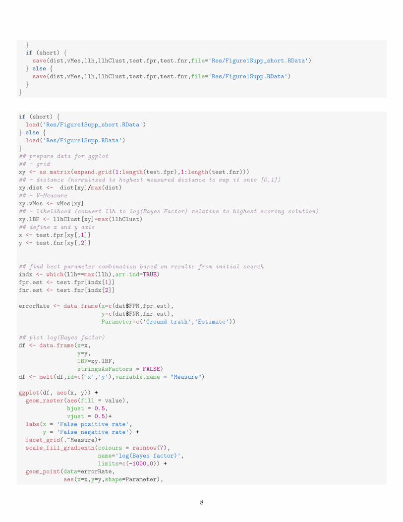
2.2 Supplementary Figure 1

Next, we test if these results can be reproduced on a data set with very low false positive rates (10−5). We start again bysimulating a data set, run the inference and plot the results.

## simulate Data set

set.seed(8)

dat <- simulateData(N.cells = 20,

N.clones = 10,

N.unobs = 2,

N.sites = 200,

6

FPR = 10^(-5),

FNR = 0.1,

p.missing = 0.2,


Then we run the oncoNEM inference algorithms over a grid of parameter combinations and assess the inferred solutions interms of likelihood, pairwise cell shortest path distance to ground truth and V-measure compared to ground truth.

if (short) {file4Exists <- file.exists('Res/Figure1Supp_short.RData')

} else {file4Exists <- file.exists('Res/Figure1Supp.RData')

}if (!file4Exists) {

## define parameter grid


if (short) {test.fpr <- test.fpr[2:11]

test.fnr <- test.fnr[2:11]

}

## initialize matrices to store performance results

dist <- vMes <- llh <- llhClust <- matrix(0,nrow=length(test.fpr),

ncol=length(test.fnr))

## run oncoNEM over parameter grid

for (i.alpha in 1:length(test.fpr)) {for (i.beta in 1:length(test.fnr)) {

## run oncoNEM


FPR=test.fpr[i.alpha],

FNR=test.fnr[i.beta])



oNEM.expanded <- expandOncoNEM(oNEM,

delta=100,

epsilon=10,

checkMax=1000,

app=TRUE)

# cluster

oncoTree <- clusterOncoNEM(oNEM.expanded,

epsilon=10)

# relabel cells to make things comparable



## measure performance

dist[i.alpha,i.beta] <- treeDistance(tree1 = dat,tree2=oncoTree)

vMes[i.alpha,i.beta] <- vMeasure(trueClusters = dat$clones,


llh[i.alpha,i.beta] <- oNEM$best$llh

llhClust[i.alpha,i.beta] <- oncoTree$llh

}

7

}if (short) {

save(dist,vMes,llh,llhClust,test.fpr,test.fnr,file='Res/Figure1Supp_short.RData')

} else {save(dist,vMes,llh,llhClust,test.fpr,test.fnr,file='Res/Figure1Supp.RData')

}}

if (short) {load('Res/Figure1Supp_short.RData')

} else {load('Res/Figure1Supp.RData')

}## prepare data for ggplot

## - grid

xy <- as.matrix(expand.grid(1:length(test.fpr),1:length(test.fnr)))

## - distance (normalized to highest measured distance to map it onto [0,1])

xy.dist <- dist[xy]/max(dist)

## - V-Measure

xy.vMes <- vMes[xy]

## - likelihood (convert llh to log(Bayes Factor) relative to highest scoring solution)

xy.lBF <- llhClust[xy]-max(llhClust)

## define x and y axis

x <- test.fpr[xy[,1]]

y <- test.fnr[xy[,2]]

## find best parameter combination based on results from initial search




errorRate <- data.frame(x=c(dat$FPR,fpr.est),

y=c(dat$FNR,fnr.est),

Parameter=c('Ground truth','Estimate'))

## plot log(Bayes factor)


y=y,

lBF=xy.lBF,




geom_raster(aes(fill = value),

hjust = 0.5,

vjust = 0.5)+





name='log(Bayes factor)',

limits=c(-1000,0)) +



8

colour="black",

bg="white",

size=4) +








aspect.ratio = 1)

## plot V-measure and Distance


y=y,

Distance=xy.dist,

vMeasure=xy.vMes,




geom_raster(aes(fill = value)) +





name='Distance/V-measure',

limits=c(0,1)) +



colour="black",

bg="white",

9

size=4) +








aspect.ratio = 1)

The estimated FPR is 0.01 (true value is 10−5), the estimated FNR is 0.115 (true value is 0.1). Note that the lowest falsepositive rate used for the parameter estimation was 0.01.

10

3 Parameter estimation accuracy and method comparison

We start by defining the default parameters and the variable parameters for our method comparison study:

## default parameters

n.sites <- 200 ## Number of mutation sites

n.clones <- 10 ## Number of clones

n.cells <- 20 ## Number of sequenced cells

n.unobs <- 0 ## Number of clones in tree that are unobserved

p.missing <- 0.2 ## Fraction of missing values

fpr <- 0.2 ## False positive rate

fnr <- 0.1 ## False negative rate

n.rep <- 5 ## Number of replicates

## simulation parameters that are varied

vary <- c("FNR","FPR","sites","clones","unobs","cells","mis")

## vary FNR

v.FNR <- c(0.05,0.1,0.2,0.3)

## vary FPR

v.FPR <- c(0.05,0.1,0.2,0.3)

## additional simulation parameter

FPRlow <- 10^-5

## vary N sites

v.sites <- c(50,100,200,300)

## vary N clones

v.clones <- c(1,5,10,20)

## vary N unobserved

v.unobs <- c(1,2,3,4)

## vary N cells per clone

v.cells <- c(1,2,3,5)*n.clones

## vary fraction of missing values

v.mis <- c(0.1,0.2,0.3,0.4)

dir.create('SimData',showWarnings = FALSE)

save(list = c('n.sites','n.clones','n.cells','n.unobs','n.rep','p.missing',

'fpr','fnr','v.FNR','v.FPR','v.sites','v.clones','v.unobs',

'v.cells','v.mis','vary','FPRlow'),

file='SimData/params.RData')

Next we simulate 5 data sets for each varied simulation parameter.

set.seed(7)

## vary FNR

for (i.FNR in 1:length(v.FNR)) {for (i.rep in 1:n.rep) {

dat <- simulateData(N.cells = n.cells,

N.clones = n.clones,

N.unobs = n.unobs,

N.sites = n.sites,

11

FPR = fpr,

FNR = v.FNR[i.FNR],

p.missing = p.missing,


## add normal cell to root

dat$D <- cbind('0'=rep(0,nrow(dat$D)),dat$D)

dat$clones[[1]] <- 0

## save

save(dat,file=paste0('SimData/v_FNR-',v.FNR[i.FNR],'_rep',i.rep,'.RData'))

}}

## vary FPR

for (i.FPR in 1:length(v.FPR)) {for (i.rep in 1:n.rep) {



N.unobs = n.unobs,

N.sites = n.sites,

FPR = v.FPR[i.FPR],

FNR = fnr,






## save

save(dat,file=paste0('SimData/v_FPR-',v.FPR[i.FPR],'_rep',i.rep,'.RData'))

}}

## vary N sites

for (i.sites in 1:length(v.sites)) {for (i.rep in 1:n.rep) {



N.unobs = n.unobs,

N.sites = v.sites[i.sites],

FPR = fpr,

FNR = fnr,






## save

save(dat,file=paste0('SimData/v_sites-',v.sites[i.sites],'_rep',i.rep,'.RData'))

}}

## vary N clones

for (i.clones in 1:length(v.clones)) {for (i.rep in 1:n.rep) {


N.clones = v.clones[i.clones],

N.unobs = n.unobs,

12

N.sites = n.sites,

FPR = fpr,

FNR = fnr,






## save

save(dat,file=paste0('SimData/v_clones-',v.clones[i.clones],'_rep',i.rep,'.RData'))

}}


for (i.unobs in 1:length(v.unobs)) {for (i.rep in 1:n.rep) {dat <- simulateData(N.cells = n.cells,


N.unobs = v.unobs[i.unobs],

N.sites = n.sites,

FPR = fpr,

FNR = fnr,






## save

save(dat,file=paste0('SimData/v_unobs-',v.unobs[i.unobs],'_rep',i.rep,'.RData'))

}}


for (i.cells in 1:length(v.cells)) {for (i.rep in 1:n.rep) {

dat <- simulateData(N.cells = v.cells[i.cells],


N.unobs = n.unobs,

N.sites = n.sites,

FPR = fpr,

FNR = fnr,






## save

save(dat,file=paste0('SimData/v_cells-',v.cells[i.cells],'_rep',i.rep,'.RData'))

}}

for (i.mis in 1:length(v.mis)) {for (i.rep in 1:n.rep) {dat <- simulateData(N.cells = n.cells,


N.unobs = n.unobs,

13

N.sites = n.sites,

FPR = fpr,

FNR = fnr,

p.missing = v.mis[i.mis],





## save

save(dat,file=paste0('SimData/v_mis-',v.mis[i.mis],'_rep',i.rep,'.RData'))

}}

In addition we simulate data sets with extremely low numbers of false positive.

for (i.rep in 1:n.rep) {dat <- simulateData(N.cells = n.cells,


N.unobs = n.unobs,

N.sites = n.sites,

FPR = FPRlow,

FNR = fnr,






## save

save(dat,file=paste0('SimData/v_FPR-',FPRlow,'_rep',i.rep,'.RData'))

}v.FPR <- c(FPRlow,v.FPR)

Then we infer trees using oncoNEM and the three baseline methods. For the short version of this script, only one replicateand one setting per simulation parameter is used.

if (short) {n.rep <- 1

for (varyX in vary) {v.X <- get(paste0('v.',varyX))

assign(paste0('v.',varyX),v.X[3])

}}

We start by running oncoNEM with and without parameter estimation.

dir.create('Res',showWarnings = FALSE)

dir.create('Res/MethodComparison',showWarnings = FALSE)

## vary FNR

## vary FPR

## vary N sites

## vary N clones



## vary fraction of missing values

14


for (i.vary in 1:length(v.X)) {

for (i.rep in 1:n.rep) {

if (!file.exists(paste0('Res/MethodComparison/oncoNEM_result_v_',varyX,

'-',v.X[i.vary],'_rep',i.rep,'.RData'))) {

## load Data

load(paste0('SimData/v_',varyX,'-',v.X[i.vary],'_rep',i.rep,'.RData'))

## -----------------------------------------------------------------------

## estimate Parameters


llh <- matrix(0,nrow=length(test.fpr),ncol=length(test.fnr))

for (i.fpr in 1:length(test.fpr)) {for (i.fnr in 1:length(test.fnr)) {

## initialize oncoNEM


FPR=test.fpr[i.fpr],

FNR=test.fnr[i.fnr])

## Run search algorithm until best tree has not changed for at least

## delta steps.


llh[i.fpr,i.fnr] <- oNEM$best$llh

}}rm(oNEM)

## find best parameter combination




## -----------------------------------------------------------------------

## Run oncoNEM with estimated Parameters


oNEM.est <- oncoNEM$new(Data=dat$D,

FPR=fpr.est,

FNR=fnr.est)


## delta steps.

oNEM.est$search(delta=200)


oNEM.est.expanded <- expandOncoNEM(oNEM.est,epsilon = 10,delta = 200)

rm(oNEM.est)

# cluster

oncoTree.est <- clusterOncoNEM(oNEM.est.expanded, epsilon=10)

rm(oNEM.est.expanded)

# relabel cells from column indices to cell indices as in ground truth

# tree

15

oncoTree.est$clones <- relabelCells(clones = oncoTree.est$clones,


## -----------------------------------------------------------------------

## As comparison run oncoNEM with true parameters



FPR=dat$FPR.effective,

FNR=dat$FNR)

## Run search algorithm



oNEM.expanded <- expandOncoNEM(oNEM,epsilon = 10,delta=200)

rm(oNEM)

# cluster

oncoTree <- clusterOncoNEM(oNEM.expanded, epsilon=10)

rm(oNEM.expanded)

# relabel cells from column indices to cell indices



## -----------------------------------------------------------------------

## save inference results so far

ssave(c('llh','fpr.est','fnr.est','oncoTree.est','oncoTree'),

file=paste0('Res/MethodComparison/oncoNEM_result_v_',varyX,

'-',v.X[i.vary],'_rep',i.rep,'.RData'))

}}

}}

Next, we run the BitPhylogeny inference.

dir.create('Res/BitPhylo_Output/',recursive = TRUE,showWarnings = FALSE)

#setup parallel backend to use 8 processors

cl<-makeCluster(4)

registerDoParallel(cl)


resultsExist <- sapply(paste0(rep(paste0('Res/BitPhylo_Output/v_',varyX,'-',v.X),each=n.rep),'_rep',

1:n.rep,'.csv/treescripts/tree-freq.csv'),

file.exists)

if (!all(resultsExist)) {#number of iterations

iters<-n.rep*length(v.X)

#loop

ls<-foreach(i=1:iters) %dopar% {library("bitphylogenyR")

16

i.X <- ceiling(i/n.rep)

i.rep <- i-(i.X-1)*n.rep

load(paste0('SimData/v_',varyX,'-',v.X[i.X],'_rep',i.rep,'.RData'))

# save data to file -> must be cells x sites

write.csv(t(dat$D[,order(as.numeric(colnames(dat$D)))]),

file=paste0('SimData/v_',varyX,'-',v.X[i.X],'_rep',i.rep,'.csv'),

row.names=FALSE)

# run bitphyloR

bitphyloR(fin = paste0('SimData/v_',varyX,'-',v.X[i.X],'_rep',i.rep,'.csv'),

fout='Res/BitPhylo_Output/',

contains_true_label=FALSE,

n=50000,

b=30000,

t=5,

mode='mutation')

}}

}

stopCluster(cl)

To be able evaluate the performance measures for BitPhylogeny later in this script, we define a function that identifies thebest BitPhylogeny tree.

getBitPhyloTree <- function(dir) {## Choose unique node num for which freq is highest.

treeFreq <- read.csv(file = paste0(dir,'/treescripts/tree-freq.csv'))

numNodes <- treeFreq$unique_node_num[which.max(treeFreq$freq)]

## read in corresponding tree

g <- read.graph(file = paste0(dir,'/treescripts/nodes-',numNodes,'.graphml'),

format = "graphml")

clones <- lapply((strsplit(V(g)$members,split = " ")),function(x) as.numeric(x))

V(g)$name <- 1:vcount(g)

return(list(g=g,clones=clones))

}

Before we run the other four baseline methods, we define functions for (i) likelihood optimization of neighbor-joining treesas done by Hughes et al (2014) and (ii) Bayesian phylogenetic inference using MrBayes as done by Eirew et al (2015). Hier-archical clustering and k-means clustering combined with minimum-spanning tree reconstruction are both implemented in theBitphylogeny R package.

## (i) likelihood optimization of NJ tree

bin_to_char <- function(x,seed=7) {## Convert a binary genotype matrix to a character matrix, by randomly assigning

## reference and mutant alleles to each site.

## Missing values are encoded using the IUPAC ambiguity code

## input: x - binary genotype matrix where each column corresponds to an SNV and

## each row corresponds to a cell

## output: character genotype matrix where each SNV has now a randomly assigned

## wt allele and mutant allele

17

set.seed(seed)

## IUPAC ambiguity code for two letters

ambigCode <- c(m='ac',m='ca',r='ag',r='ga',w='at',w='ta',s='cg',s='gc',

y='ct',y='tc',k='gt',k='tg')

## randomly assign wildtype+ref allele to convert 1/0 matrix to characters

for (i in 1:ncol(x)) {gtyp <- sample(x = c('a','c','g','t'), size=2, replace = FALSE)

x[x[,i]==0,i] <- gtyp[1] ## wt genotype

x[x[,i]==1,i] <- gtyp[2] ## mutant genotype

x[x[,i]==2,i] <- names(ambigCode)[paste(gtyp,collapse="")==ambigCode] # ambig genotype

}

return(x)

}

clusterPhylo <- function(phylo,K) {## Infer cell clusters in the phylogenetic tree by hierarchical clustering of the distance matrix

## convert tree from class phylo to class igraph

g <- graph.edgelist(el=phylo$edge)

E(g)$weight <- phylo$edge.length

## extract distance matrix for cells

dm <- shortest.paths(g)

rownames(dm) <- colnames(dm) <- V(g)

dis <- as.dist(dm[as.character(1:nrow(x)),as.character(1:nrow(x))])

## apply hierarchical clustering to the distance matrix of the optimized NJtree to infer clusters

hc_cand <- lapply(K, function(ii) cutree(hclust(dis), ii))

hc_silhouette_res <- sapply(1:length(K), function(ii) summary(silhouette(hc_cand[[ii]],

dis))$avg.width)

## choose number of clusters that maximize silhouette score

idx <- which.max(hc_silhouette_res)

hc_label <- hc_cand[[idx]]

## return cluster labels

return(hc_label)

}

## Infers cluster labels for each cell using likelihood optimization of a neighbour joining tree.

get_label_lo <- function (x,K=2:(nrow(x)-1)) {## input: x - binary genotype matrix where each row corresponds to an SNV and

## each column corresponds to a cell

## output: vector containing the cluster label for each cell

## convert binary genotype matrix to character matrix by randomly assigning reference and mutant allele

xChar <- bin_to_char(x)

## Step 1: Build NJ tree

## Convert format of genotype matrix for dist.dna function

x.DNAbin <- as.DNAbin(xChar)

## Calculated pairwise distances between cells using a generalized Kimura model

dd <- dist.dna(x.DNAbin,model="K81",pairwise.deletion = TRUE)

if (any(is.infinite(dd)|is.nan(dd))) { ## test if distance calculation failed for any entries

return(NA) ## NaN/Inf cause error in likelihood optimization

}

18

## infer tree using modified neighbour-joining algorithm

NJTree <- bionjs(X = dd)

## Step 2: Perform ML-optimization

## Convert format of genotype matrix for likelihood optimization

pD <- phyDat(xChar,type="DNA")

## compute likelihood of NJTree given genotypes

suppressWarnings(x.pml <- pml(NJTree,data=pD,model='GTR'))

## Perform likelihood optimization under a generalized time reversible (GTR) substitution model

x.optPml <- optim.pml(x.pml,model='GTR')

## Step 3: Infer clusters from estimated tree

lo_label <- clusterPhylo(x.optPml$tree,K=K)

return(lo_label)

}

## (ii) Bayesian phylogenetic inference using MrBayes

writeNexus <- function(D,fileNameBase) {## D - columns correspond to species, rows correspond to sites

D <- apply(D,1,as.character)

## code ambiguous sites

if (any(is.na(D))) {D[is.na(D)] <- '{0,1}'

} else if (any(D==2)) {D[D=='2'] <- '{0,1}'

}colnames(D) <- 1:ncol(D)

## write to file in nexus format

write.nexus.data(x=D,file=paste0(fileNameBase,'.nex'))

## change data type from DNA to Restriction

system(command = paste0("awk '{ gsub(\"DNA\",\"Restriction\"); print $0 }' ",

fileNameBase,".nex > ",fileNameBase,"2.nex"))

## rename file

system(command = paste0("mv ",fileNameBase,"2.nex ", fileNameBase,".nex"))

}

MrBayes <- function(fileNameBase,ngen,verbose=FALSE,seeds=sample(100,2)) {## write MrBayes script

fileConn <- file(paste0(fileNameBase,"MrBayes.txt"))

writeLines(c("set autoclose=yes nowarn=yes;",

paste0("set seed=",seeds[1]," swapseed=",seeds[2],";"),

## load data

paste0("execute ",fileNameBase,".nex;"),

## set parameters

"lset rates=equal coding=all;",

"prset statefreqpr=Dirichlet(1,1);",

## run inference

paste0("mcmc nruns=2 ngen=",format(ngen,scientific=FALSE)," burninfrac=0.5;"),

"sump;",

"sumt;",

"quit;"), fileConn)

close(fileConn)

## run MrBayes

if (verbose) {

19

system(command = paste0("mpirun -np 4 mb ", fileNameBase,"MrBayes.txt"))

} else {system(command = paste0("mpirun -np 4 mb ", fileNameBase, "MrBayes.txt"),ignore.stdout=TRUE)

}

## read consensus tree from MrBayes output file

ct <- read.nexus(paste0(fileNameBase,".nex.con.tre"))

## return consensus tree

return(ct)

}

## run Bayesian phylogenetic inference

get_label_mb <- function(x,fileNameBase,ngen,K=2:(nrow(x)-1),seeds=sample(100,2)) {

writeNexus(t(x),fileNameBase=fileNameBase)

ct <- MrBayes(fileNameBase,ngen=ngen,seeds=seeds)

MrBayes_labels <- clusterPhylo(ct,K=K)

return(MrBayes_labels)

}

We run the analysis for four of the five the remaining four baseline methods and evaluate the oncoNEM and BitPhylogenyoutput in terms of V-measure and pairwise-cell shortest path distance.

dir.create('Res/MrBayes',showWarnings = FALSE)

set.seed(1)


## initialize list to store results

RES <- vector("list")


## initialize matrices to store results

vMes <- dist <- matrix(0,nrow=n.rep,ncol=7)

colnames(vMes) <- colnames(dist) <- c("oncoNEM.est","oncoNEM",

"hc","kc","lo","mb","bitPhylogeny")

for (i.rep in 1:n.rep) {## load Data


## -----------------------------------------------------------------------

## Run baseline methods hc and kc + MST, likelihood optimization of NJ tree (lo),

## and Bayesian Inference using MrBayes (mb)

## reformat Data for other methods

Data <- dat$D

x <- t(Data[,order(as.numeric(colnames(Data)))])

## HIERARCHICAL CLUSTERING

hc <- get_label_hc(x,K=2:(nrow(x)-1))

hcTree <- list(g=get_mst(hc$genotype),clones=split(as.numeric(names(hc$label)),

f=hc$label))

20

## K-CENTROIDS

kc <- get_label_kc(x,K=2:(nrow(x)-1))

kcTree <- list(g=get_mst(kc$genotype),clones=split(as.numeric(names(kc$label)),

f=kc$label))

## likelihood optimization

lo <- get_label_lo(x,K=2:(nrow(x)-1))

if (all(!is.na(lo))) {lo_clones <- split(0:(length(lo)-1),f=lo)

} else {lo_clones <- NULL

}

## Bayesian phylogenetic inference with MrBayes

if (file.exists(paste0('Res/MrBayes/v_',varyX,'-',v.X[i.vary],'_rep',i.rep,'.nex.con.tre'))) {ct <- read.nexus(paste0('Res/MrBayes/v_',varyX,'-',v.X[i.vary],'_rep',i.rep,'.nex.con.tre'))

mb <- clusterPhylo(ct,K=2:(nrow(x)-1))

} else {mb <- get_label_mb(x,fileNameBase=

paste0('Res/MrBayes/v_',varyX,'-',v.X[i.vary],'_rep',i.rep),

ngen=10^7,

K=2:(nrow(x)-1))

}mb_clones <- split(0:(length(mb)-1),f=mb)

## -----------------------------------------------------------------------

## load oncoNEM results

load(paste0('Res/MethodComparison/oncoNEM_result_v_',varyX,'-',v.X[i.vary],

'_rep',i.rep,'.RData'))

## -----------------------------------------------------------------------

## load BitPhylogeny results

if (file.exists(paste0('Res/BitPhylo_Output/v_',varyX,'-',v.X[i.vary],

'_rep',i.rep,'.csv'))) {# extract BITPHYLOGENY results

bitTree <-

getBitPhyloTree(dir = paste0('Res/BitPhylo_Output/v_',varyX,'-',v.X[i.vary],

'_rep',i.rep,'.csv'))

} else {bitTree <- NULL

}

## -----------------------------------------------------------------------

## summarize results

# vMeasure (all baseline methods)

vMes[i.rep,"hc"] <- vMeasure(trueClusters = dat$clones,

predClusters = hcTree$clones)

vMes[i.rep,"kc"] <- vMeasure(trueClusters = dat$clones,

predClusters = kcTree$clones)

if (is.null(lo_clones)) { ## if lo failed

vMes[i.rep,"lo"] <- NA

} else {vMes[i.rep,"lo"] <- vMeasure(trueClusters = dat$clones,

predClusters = lo_clones)

21

}vMes[i.rep,"mb"] <- vMeasure(trueClusters = dat$clones,

predClusters = mb_clones)

vMes[i.rep,"oncoNEM.est"] <- vMeasure(trueClusters = dat$clones,

predClusters = oncoTree.est$clones)

vMes[i.rep,"oncoNEM"] <- vMeasure(trueClusters = dat$clones,


vMes[i.rep,"bitPhylogeny"] <- vMeasure(trueClusters = dat$clones,

predClusters = bitTree$clones)

# Distance (not lo and mb)

dist[i.rep,"hc"] <- treeDistance(tree1 = dat, tree2 = hcTree,

root2 = which(sapply(hcTree$clones,

function(x) any(x==0))))

dist[i.rep,"kc"] <- treeDistance(tree1 = dat, tree2 = kcTree,

root2 = which(sapply(kcTree$clones,

function(x) any(x==0))))

dist[i.rep,"lo"] <- NA

dist[i.rep,"mb"] <- NA

dist[i.rep,"oncoNEM.est"] <- treeDistance(tree1 = dat,

tree2=oncoTree.est)

dist[i.rep,"oncoNEM"] <- treeDistance(tree1 = dat,

tree2=oncoTree)

dist[i.rep,"bitPhylogeny"] <- treeDistance(tree1 = dat,

tree2 = bitTree)

}

RES$vMES[[i.vary]] <- vMes

RES$DIS[[i.vary]] <- dist

}

## save results

save(RES,file=paste0('Res/v_',varyX,'.RData'))

}

Finally, we apply Kim and Simon’s method to the simulated data set and compare its performance with that if oncoNEM.Their method infers onocogenetic trees and does not provide the position of the single cells within the tree. Therefore, V-measureand pairwise cell shortest-path distance cannot be aplied here. Instead, we calculate the average of

a) the fraction of correctly inferred pairwise mutation orders (i.e. mutation a is upstream of mutation b or vice versa) and

b) the fraction of correctly inferred mutually exclusive mutations (i.e. mutations a and b lie on separate branches)

out of all mutations that are not in the same mutation cluster in the simulated tree. This restricition is necessary because Kimand Simon’s method does not cluster mutations.

if (!file.exists('Res/res_KimAndSimon.RData')) {

res <- as.data.frame(matrix(0,ncol=6,nrow=sum(sapply(vary,

function(x) length(get(paste0('v.',x))))*n.rep)),


colnames(res) <- c('varyX',

'v.X',

'i.rep',

'subsetPerformance',

22

'mutExclusivePerformance',

'overallPerformance')

counter=0



for (i.rep in 1:n.rep) {counter <- counter + 1


## Run Kim and Simon's method

kimdir <- paste0('Res/Kim/MethodComparison/v_',varyX,'-',v.X[i.vary],'_rep',i.rep)

dir.create(kimdir,recursive = TRUE,showWarnings = FALSE)

## order data by cell index

mc <- dat$D[,order(as.numeric(colnames(dat$D)))]

Gob <- inferKimAndSimon(mc=mc, fdr= dat$FPR, ado = dat$FNR, fileNameBase = kimdir)

## Load OncoNEM results

load(paste0('Res/MethodComparison/oncoNEM_result_v_',varyX,'-',v.X[i.vary],

'_rep',i.rep,'.RData'))

## Calculate transitive closure of Kim & Simon's inferred mutation graph

el.Kim <- apply(Gob$edgeList,1,as.numeric)

tc.Kim <- transitiveClosure(el.Kim)

## order by mutation timing from early to late

tc.Kim <- tc.Kim[order(dat$theta),order(dat$theta)]

## Calculate transitive closure of inferred oncoNEM (cell) tree

el.OncoNEM <- get.edgelist(oncoTree.est$g)

tc.OncoNEM <- transitiveClosure(el.OncoNEM)

# extend to mutations

p_theta.est <- oncoNEMposteriors(tree=oncoTree.est$g, clones=oncoTree.est$clones,

Data=dat$D,FPR=fpr.est,FNR=fnr.est)$p_theta

theta.est <- apply(p_theta.est,1,which.max)

tc.OncoNEM <- tc.OncoNEM[theta.est,theta.est]

## order by mutation timing

tc.OncoNEM <- tc.OncoNEM[order(dat$theta),order(dat$theta)]

## Calculate transitive closure of simulated cell tree

el.Sim <- get.edgelist(dat$g)

tc.Sim <- transitiveClosure(el.Sim)

# extend to mutations

tc.Sim <- tc.Sim[dat$theta,dat$theta]

## order by mutation timing

tc.Sim <- tc.Sim[order(dat$theta),order(dat$theta)]

## To asses performance we only consider mutations that belong to different clusters in the

## simulated trees as Kim & Simon's method does not perform clustering

mutInDiffClust <- outer(dat$theta,dat$theta, FUN='!=')

23

mutInDiffClust <- mutInDiffClust[order(dat$theta),order(dat$theta)]

mutInDiffClust[lower.tri(mutInDiffClust)] <- FALSE

## Kim and Simon's method

## Calculate what fraction of subset relationships is correctly identified

res$KS.subsetPerformance[counter] <- sum((tc.Sim==tc.Kim)[mutInDiffClust&tc.Sim==1])/

sum(mutInDiffClust&tc.Sim==1)

## Calculate what fraction of mutually exclusive mutations is correctly identified

res$KS.mutExclusivePerformance[counter] <- sum((tc.Sim==tc.Kim)[mutInDiffClust&tc.Sim!=1])/

sum(mutInDiffClust&tc.Sim!=1)

## oncoNEM

## Calculate what fraction of subset relationships is correctly identified

res$ON.subsetPerformance[counter] <- sum((tc.Sim==tc.OncoNEM)[mutInDiffClust&tc.Sim==1])/

sum(mutInDiffClust&tc.Sim==1)

## Calculate what fraction of mutually exclusive mutations is correctly identified

res$ON.mutExclusivePerformance[counter] <- sum((tc.Sim==tc.OncoNEM)[mutInDiffClust&tc.Sim!=1])/

sum(mutInDiffClust&tc.Sim!=1)

res[counter,c('varyX','v.X','i.rep')] <- c(varyX,v.X[i.vary],i.rep)

}## Average those 2 performance measures

res$KS.overallPerformance <- 1/2*(res$KS.subsetPerformance+res$KS.mutExclusivePerformance)

res$ON.overallPerformance <- 1/2*(res$ON.subsetPerformance+res$ON.mutExclusivePerformance)

}}

save(res,file = 'Res/res_KimAndSimon.RData')

}

24

3.1 Figure 3B

For every simulation run we extract the error rates that were estimated by oncoNEM and store them in a data frame with allother simulation parameters.

estimatedParams <- data.frame(varyX=character(),

v.X=numeric(),

rep=numeric(),

trueFPR=numeric(),

estFPR=numeric(),

trueFNR=numeric(),

estFNR=numeric(),




for (i.rep in 1:n.rep) {## load estimated oncoNEM

load(paste0('Res/MethodComparison/oncoNEM_result_v_',varyX,'-',

v.X[i.vary],'_rep',i.rep,'.RData'))

if (varyX=='FPR') {estimatedParams[nrow(estimatedParams)+1,] <-

data.frame(varyX=varyX,

v.X=v.X[i.vary],

rep=i.rep,

trueFPR=v.FPR[i.vary],

estFPR=fpr.est,

trueFNR=fnr,

estFNR=fnr.est,stringsAsFactors = FALSE)

} else if (varyX=='FNR') {estimatedParams[nrow(estimatedParams)+1,] <-


v.X=v.X[i.vary],

rep=i.rep,

trueFPR=fpr,

estFPR=fpr.est,

trueFNR=v.FNR[i.vary],

estFNR=fnr.est,


} else {estimatedParams[nrow(estimatedParams)+1,] <-


v.X=v.X[i.vary],

rep=i.rep,

trueFPR=fpr,

estFPR=fpr.est,

trueFNR=fnr,

estFNR=fnr.est,


}}

}}

25

Then we plot the results using ggplot2.

## prepare data frame for ggplot2

df <- melt(estimatedParams,id.vars =c('varyX','v.X','rep','trueFPR','trueFNR'),

measure.vars = c('estFPR','estFNR'))

## make single column for ground truth parameter that contains true FPR if the

## measured variable is estFPR and that contains true FNR if the measured

## variable is est FNR>

df$trueValue <- df$trueFPR

df$trueValue[df$variable=='estFNR'] <- df$trueFNR[df$variable=='estFNR']

## add column for faceting

df$variedParam <- paste0(df$varyX,'=',df$v.X)

## set order of facets

df$variedParam <- factor(df$variedParam,levels=unique(df$variedParam))

# if (short) {# df£variedParam <- factor(df£variedParam,levels=

# paste0(vary,"=",

# unlist(lapply(paste0('v.',vary),get))))

# } else {# df£variedParam <- factor(df£variedParam,levels=

# paste0(rep(vary,each=4),"=",

# unlist(lapply(paste0('v.',vary),get))))

# }

## set colour of dots to same as for this method in the method comparison plot

df$col <- factor(x=2,levels=1:5)

## make ggplot

ggplot(df,aes(x=rep,y=value,color=col)) +

stat_summary(mapping=aes(x=3,y=trueValue),

fun.y=mean,

fun.ymin=mean,

fun.ymax=mean,

geom="crossbar",

width = 5,

fatten = 1,

size=1,

colour=gg_color_hue(6)[4]) +

geom_point(alpha=1) +

facet_grid(variable~variedParam,scales="free_y") +

scale_colour_manual(values=gg_color_hue(7)[2:3]) +

scale_y_continuous( breaks=test.fpr,

minor_breaks=NULL,

limits=c(0,0.5)) +

scale_x_continuous(limits=c(0.5,n.rep+0.5)) +

theme_bw()+

theme(axis.ticks.x = element_blank(),

axis.text.x = element_blank(),

axis.title.x = element_blank(),

axis.title.y = element_blank(),

panel.grid.minor.x=element_blank(),

panel.grid.major.x=element_blank(),

panel.grid.major = element_line(size = 1),


legend.position="none")

26

FNR=0.05FNR=0.1FNR=0.2FNR=0.3FPR=1e−05FPR=0.05FPR=0.1FPR=0.2FPR=0.3 sites=50sites=100sites=200sites=300clones=1clones=5clones=10clones=20unobs=1 unobs=2 unobs=3 unobs=4 cells=10 cells=20 cells=30 cells=50 mis=0.1 mis=0.2 mis=0.3 mis=0.4

0.0100.0450.0800.1150.1500.1850.2200.2550.2900.3250.3600.3950.4300.4650.500

0.0100.0450.0800.1150.1500.1850.2200.2550.2900.3250.3600.3950.4300.4650.500

estFP

RestF

NR

The results show that oncoNEM estimates model parameters accurately over a wide range of simulation settings.

27

3.2 Figure 5

Next we summarize the performance results of all methods but Kim and Simon’s in a single data frame which we then use forplotting. Note that, in order to make the range of values more similar between the different simulated data sets, we normalizethe distances for the number of cells in the trees.

## initialize df to store results in plotting format

summary <- data.frame(variedParam=factor(),

Method=character(),

variable=character(),

value=numeric())

for (varyX in vary) {

## read data for every varied parameter

load(paste0('Res/v_',varyX,'.RData'))

## change data structure

dist <- as.data.frame(cbind(RES$DIS[[1]],variedParam=get(paste0('v.',varyX))[1]))

vMes <- as.data.frame(cbind(RES$vMES[[1]],variedParam=get(paste0('v.',varyX))[1]))

if (!short){for (i in 2:length(RES$DIS)) {dist <- rbind(dist,cbind(RES$DIS[[i]],variedParam=get(paste0('v.',varyX))[i]))

vMes <- rbind(vMes,cbind(RES$vMES[[i]],variedParam=get(paste0('v.',varyX))[i]))

}}## adjust distance for number of cells

if (varyX!="cells") {dist[,1:(ncol(dist)-1)] <- dist[,1:(ncol(dist)-1)]/(((n.cells+2)*(n.cells+1))/2)

## +1 for cell added to root by treeDistance

## +1 for normal cell added to each simulated data set

} else {dist[,1:(ncol(dist)-1)] <- dist[,1:(ncol(dist)-1)]/(((dist$variedParam+2)*(dist$variedParam+1))/2)

}## melt

dist_melt <- melt(dist,id="variedParam",variable.name = "Method")

vMes_melt <- melt(vMes,id="variedParam",variable.name = "Method")

## combine distance and v-measure

res <- cbind(dist_melt,vMes_melt$value)

colnames(res)[3:4] <- c("Distance/(N*(N-1)/2)","V-measure")

## melt again

res <- melt(res,id=c('variedParam','Method'))

## set order of facets in plot

res$variedParam <- factor(paste0(varyX,'=',res$variedParam),

levels=unique(paste0(varyX,'=',res$variedParam)))

summary <- rbind(summary,res)

}

Now we plot the results of the method comparison obtained above.

## change levels

summary$Method <- factor(summary$Method,levels=c("oncoNEM","oncoNEM.est",

"bitPhylogeny","hc","kc","lo","mb"))

## remove missing values for failed inferences

summary <- summary[!is.na(summary$value),]

28

ggplot(summary[summary$variable=='Distance/(N*(N-1)/2)',], aes(x=Method,y=value))+

geom_dotplot(aes(y = value, x = Method, fill = Method , colour = Method),

binaxis = "y",

binwidth = 0.05,

stackdir = "center",

dotsize = 3,

stackratio = 0.5) +

stat_summary(fun.y=mean,

fun.ymin=mean,

fun.ymax=mean,

geom="crossbar",

width = 1,

fatten = 1,

colour='black') +

scale_y_reverse() +

facet_grid(variable~variedParam,scales="free_y")+

theme_bw() +







legend.position="bottom") +

guides(fill=FALSE)

ggplot(summary[summary$variable=='V-measure',], aes(x=Method,y=value))+

geom_dotplot(aes(y = value, x = Method, fill = Method, colour = Method),

binaxis = "y",

binwidth = 0.05,

stackdir = "center",

dotsize = 1,

stackratio = 0.5) +

stat_summary(fun.y=mean,

fun.ymin=mean,

fun.ymax=mean,

geom="crossbar",

width = 1,

fatten = 1,

colour='black') +

facet_grid(variable~variedParam) +

scale_colour_manual(values=gg_color_hue(7)) +

scale_y_continuous(limits = c(0, 1)) +

theme_bw()+







legend.position="bottom")+

guides(fill=FALSE)

29


0

1

2

3

4

Distance/(N

*(N−

1)/2)

Method oncoNEM oncoNEM.est bitPhylogeny hc kc


0.00

0.25

0.50

0.75

1.00

V−

measure

MethodoncoNEM

oncoNEM.est

bitPhylogeny

hc

kc

lo

mb

For the comparison with Kim and Simon’s method we plot the accuracy of the inferred mutation orders obtained earlier inthis section.

load('Res/res_KimAndSimon.RData')

res2 <- melt(res,

id.vars = c('varyX','v.X','i.rep'),

measure.vars = c('KS.overallPerformance','ON.overallPerformance'))

res2$variedParam <- paste0(res2$varyX,res2$v.X)

res2$variedParam <- factor(res2$variedParam,levels = unique(res2$variedParam))

ggplot(res2,aes(x=i.rep,y=value,col=variable)) +

facet_grid(.~variedParam,scales="free_x") +

geom_point(na.rm=TRUE) +

scale_y_continuous(limits=c(0,1)) +

theme_bw() +




panel.grid.minor.x = element_blank(),

panel.grid.major.x = element_blank(),

panel.grid.major.y = element_line(size = 0.3),

legend.position='bottom') +

ylab("Accuracy of mutation order")

FNR0.05 FNR0.1 FNR0.2 FNR0.3FPR1e−05FPR0.05 FPR0.1 FPR0.2 FPR0.3 sites50 sites100 sites200 sites300 clones1 clones5 clones10clones20 unobs1 unobs2 unobs3 unobs4 cells10 cells20 cells30 cells50 mis0.1 mis0.2 mis0.3 mis0.4

0.00

0.25

0.50

0.75

1.00

Acc

urac

y of

mut

atio

n or

der

variable KS.overallPerformance ON.overallPerformance

The two plots show that oncoNEM outperforms the baseline methods for all simulation scenarios but the single clone case.It consistently yields results that have a smaller distance to the ground truth and a higher V-measure and the inferred orderingof mutation is more accurate.

30

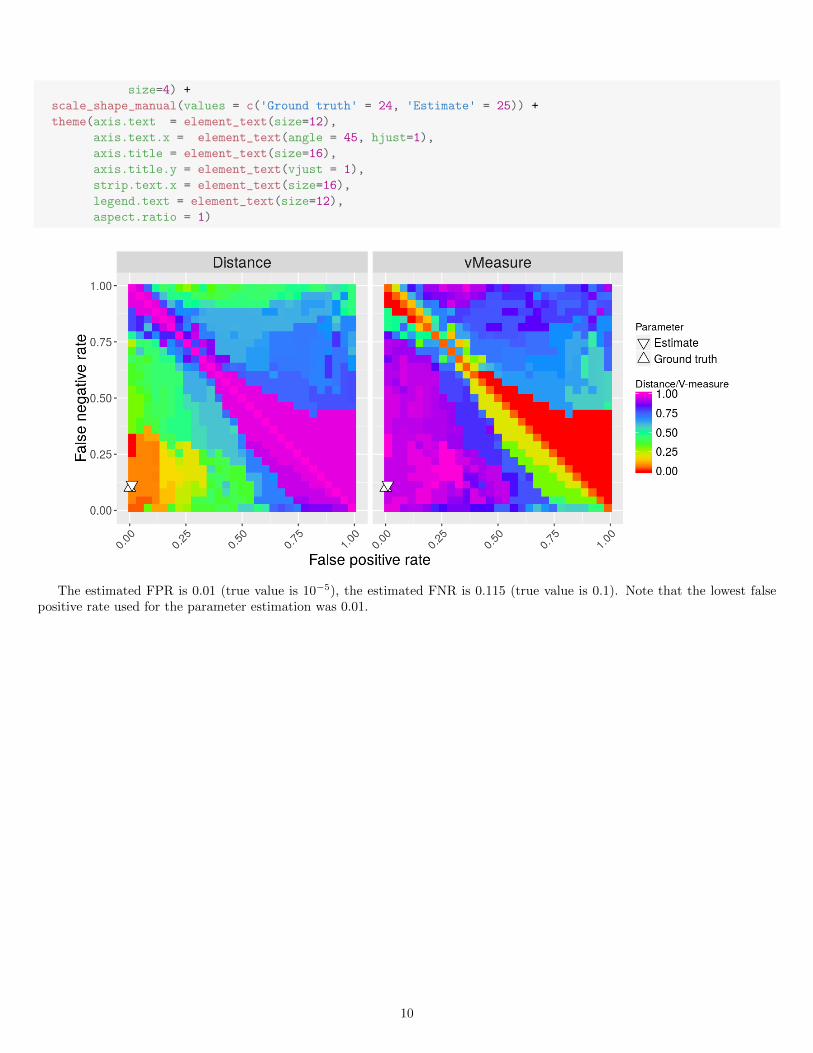
4 Dependence of oncoNEM results on threshold ε (Figure 4)

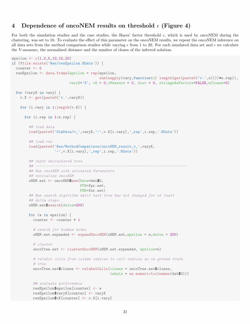
For both the simulation studies and the case studies, the Bayes’ factor threshold ε, which is used by oncoNEM during theclustering, was set to 10. To evaluate the effect of this parameter on the oncoNEM results, we repeat the oncoNEM inference onall data sets from the method comparison studies while varying ε from 1 to 20. For each simulated data set and ε we calculatethe V-measure, the normalized distance and the number of clones of the inferred solution.

epsilon <- c(1,2,5,10,15,20)

if (!file.exists('Res/resEpsilon.RData')) {counter <- 0

resEpsilon <- data.frame(epsilon = rep(epsilon,

sum(sapply(vary,function(x) length(get(paste0('v.',x))))*n.rep)),

varyX='X', vX = 0,vMeasure = 0, dist = 0, stringsAsFactors=FALSE,nClones=0)



for (i.rep in 1:n.rep) {

## load data


## load res

load(paste0('Res/MethodComparison/oncoNEM_result_v_',varyX,

'-',v.X[i.vary],'_rep',i.rep,'.RData'))

## infer unclustered tree

## -----------------------------------------------------------------------

## Run oncoNEM with estimated Parameters


oNEM.est <- oncoNEM$new(Data=dat$D,

FPR=fpr.est,

FNR=fnr.est)


## delta steps.

oNEM.est$search(delta=200)

for (e in epsilon) {counter <- counter + 1


oNEM.est.expanded <- expandOncoNEM(oNEM.est,epsilon = e,delta = 200)

# cluster

oncoTree.est <- clusterOncoNEM(oNEM.est.expanded, epsilon=e)

# relabel cells from column indices to cell indices as in ground truth

# tree

oncoTree.est$clones <- relabelCells(clones = oncoTree.est$clones,


## evaluate performance

resEpsilon$epsilon[counter] <- e

resEpsilon$varyX[counter] <- varyX

resEpsilon$vX[counter] <- v.X[i.vary]

31

resEpsilon$vMeasure[counter] <- vMeasure(trueClusters = dat$clones,

predClusters = oncoTree.est$clones)

resEpsilon$dist[counter] <- treeDistance(tree1 = dat,

tree2=oncoTree.est)

resEpsilon$nClones[counter] <- length(oncoTree.est$clones)

}rm(oNEM.est)

rm(oNEM.est.expanded)

save(resEpsilon,file='Res/resEpsilon.RData')

}}

}

}

Finally we plot these three measures as a function of epsilon for the different simulation scenarios.

load('Res/resEpsilon.RData')

## assign id for each line

resEpsilon$id <- rep(1:(nrow(resEpsilon)/length(epsilon)),each=length(epsilon))

## assign id for colouring each line by parameter setting

resEpsilon$id2 <- as.factor(unlist(lapply(vary,function(x) rep(1:length(get(paste0('v.',x))),

each=length(epsilon)*n.rep))))

## normalize distance by number of cell

resEpsilon$dist[resEpsilon$varyX!='cells'] <- resEpsilon$dist[resEpsilon$varyX!='cells']/

(((n.cells+2)*(n.cells+1))/2)

## +1 for cell added to root by treeDistance

## +1 for normal cell added to each simulated data set

nv.cells <- resEpsilon$vX[resEpsilon$varyX=='cells']

resEpsilon$dist[resEpsilon$varyX=='cells'] <- resEpsilon$dist[resEpsilon$varyX=='cells']/

(((nv.cells+2)*(nv.cells+1))/2)

resEpsilon <- melt(resEpsilon,id.vars = c('epsilon','varyX','vX','id','id2'),

measure.vars = c('vMeasure','nClones'))

levels(resEpsilon$variable) <- c('V-measure','# clones')

ggplot(resEpsilon,aes(x=epsilon,y=value,colour=id2)) +

geom_line(aes(group=id)) +

facet_grid(variable~varyX,scales="free_y") +

scale_color_discrete(name="Parameter\nSetting") +

expand_limits(y=0) +

geom_vline(xintercept=10,linetype=2) +

theme_bw() +

theme(axis.title.y = element_blank(),legend.position='bottom')

32

cells clones FNR FPR mis sites unobs

0.00

0.25

0.50

0.75

1.00

0

10

20

30

V−

measure

# clones

5 10 15 20 5 10 15 20 5 10 15 20 5 10 15 20 5 10 15 20 5 10 15 20 5 10 15 20epsilon

ParameterSetting

1 2 3 4 5

In all simulation scenarios the number of clones is largely independent of epsilon, unless for unreasonably small choices ofε < 5. The threshold for ε used throughout the paper is 10 (dashed line), and thus well within the stable range.

33

5 Session Info

sessionInfo()

## R version 3.2.3 (2015-12-10)

## Platform: x86_64-pc-linux-gnu (64-bit)

## Running under: Ubuntu 14.04.3 LTS

##

## locale:

## [1] LC_CTYPE=en_GB.UTF-8 LC_NUMERIC=C

## [3] LC_TIME=en_GB.UTF-8 LC_COLLATE=en_GB.UTF-8

## [5] LC_MONETARY=en_GB.UTF-8 LC_MESSAGES=en_GB.UTF-8

## [7] LC_PAPER=en_GB.UTF-8 LC_NAME=C

## [9] LC_ADDRESS=C LC_TELEPHONE=C

## [11] LC_MEASUREMENT=en_GB.UTF-8 LC_IDENTIFICATION=C

##

## attached base packages:

## [1] parallel stats graphics grDevices utils datasets methods

## [8] base

##

## other attached packages:

## [1] KimAndSimon_0.0.0.9000 RBGL_1.44.0 graph_1.48.0

## [4] phangorn_1.99.14 ape_3.3 cluster_2.0.3

## [7] doParallel_1.0.10 iterators_1.0.8 foreach_1.4.3

## [10] bitphylogenyR_0.99 igraph_1.0.1 rPython_0.0-5

## [13] RJSONIO_1.3-0 reshape2_1.4.1 ggplot2_2.0.0

## [16] oncoNEM_1.0 Rcpp_0.12.3 knitr_1.10.5

##

## loaded via a namespace (and not attached):

## [1] formatR_1.2 plyr_1.8.3 highr_0.5

## [4] bitops_1.0-6 class_7.3-14 tools_3.2.3

## [7] digest_0.6.9 evaluate_0.7 gtable_0.2.0

## [10] nlme_3.1-123 lattice_0.20-33 Matrix_1.2-3

## [13] e1071_1.6-7 stringr_1.0.0 gtools_3.5.0

## [16] caTools_1.17.1 stats4_3.2.3 grid_3.2.3

## [19] gdata_2.17.0 magrittr_1.5 BiocGenerics_0.16.1

## [22] scales_0.4.0 gplots_2.17.0 codetools_0.2-14

## [25] nnls_1.4 riverplot_0.5 mcclust_1.0

## [28] colorspace_1.2-6 labeling_0.3 quadprog_1.5-5

## [31] KernSmooth_2.23-15 stringi_1.0-1 munsell_0.4.3

## [34] ggm_2.3

34

Supplement to OncoNEM: Inferring tumour evolution from ...10.1186/s13059-016-0929... · Supplement...

Documents

Transcript of Supplement to OncoNEM: Inferring tumour evolution from ...10.1186/s13059-016-0929... · Supplement...