ARTICLE IN PRESS

0168-9002/$ - se

doi:10.1016/j.ni

�CorrespondE-mail addr

(R.S. Romaniu

Nuclear Instruments and Methods in Physics Research A 568 (2006) 854–862

www.elsevier.com/locate/nima

Superconducting cavity driving with FPGA controller

Tomasz Czarskia, Waldemar Kopreka, Krzysztof T. Pozniaka, Ryszard S. Romaniuka,�,Stefan Simrockb, Alexander Brandtb, Brian Chasec, Ruben Carcagnoc,

Gustavo Canceloc, Timothy W. Koethd

aELHEP Laboratory, ISE, Warsaw University of Technology, PolandbDESY, Hamburg, Germany

cFERMILAB, Batavia, IL 60510, USAdRUTGERS, The State University of New Jersey, USA

Received 29 January 2006; received in revised form 25 July 2006; accepted 28 July 2006

Available online 5 September 2006

Abstract

A digital control of superconducting cavities for a linear accelerator is presented. FPGA-based controller, supported by Matlab

system, was applied. Electrical model of a resonator was used for design of a control system. Calibration of the signal path is considered.

Identification of cavity parameters has been carried out for adaptive control algorithm. Feed-forward and feedback modes were applied

in operating the cavities. Required performance has been achieved; i.e. driving on resonance during filling and field stabilization during

flattop time, while keeping reasonable level of the power consumption. Representative results of the experiments are presented for

different levels of the cavity field gradient.

r 2006 Elsevier B.V. All rights reserved.

PACS: 07.05.Dz; 07.50.�c; 29.17.+w; 29.50.+v

Keywords: TESLA cavity control; CHECHIA driving; FPGA; System identification; LLRF control

1. Introduction

Low level radio frequency (LLRF) cavity control systemis under development in order to improve regulation ofaccelerating fields in the resonators [1] (Fig. 1). Acontrolled section, powered by one klystron, may consistof many cavities. Fast amplitude and phase control of thecavity field is accomplished by modulation of signal drivingthe klystron using a vector modulator. Cavities are drivenwith 1.3ms pulses to an average accelerating gradient of25MV/m. The cavity RF signal is down converted to anintermediate frequency of 250KHz, while preserving theamplitude and phase information. ADC and DACconverters link the analog and digital parts of the systemwith a sampling interval of 1 ms. Digital signal processing is

e front matter r 2006 Elsevier B.V. All rights reserved.

ma.2006.07.063

ing author. Tel.: +48501472206.

esses: rrom@ise.pw.edu.pl, , R.Romaniuk@ise.pw.edu.pl

k).

executed in FPGA system to obtain the field vectordetection, calibration and filtering. Control feedbacksystem regulates the vector sum of the pulsed acceleratingfields in multiple cavities. FPGA-based controller stabilizesthe detected real (in-phase) and imaginary (quadrature)components of incident wave according to the given setpoint [2]. Adaptive feed forward (FF) is applied to improvethe compensation of repetitive perturbations induced bythe beam loading and by dynamic Lorentz force detuning.Control block applies the value of cavity parameters,estimated in the identification system, and generatesrequired data for the controller. A system model wasdeveloped for investigating the optimal control method ofthe cavity [3].A new control system was experimentally introduced in:

a laboratory setup of CHECHIA and ACC1 module of theVU-FEL TTF (FLASH) in DESY and A0 module inFERMILAB. CHECHIA is a horizontal test cryostat for asingle, standard TESLA 1.3GHz, superconducting cavity.

ARTICLE IN PRESS

Fig 1. Functional block diagram of LLRF cavity control system (for one cavity).

T. Czarski et al. / Nuclear Instruments and Methods in Physics Research A 568 (2006) 854–862 855

ACC1 is the first cryo-module in the TTF linac with 8cavities. A single 9-cell TESLA superconducting cavity ofthe FNPL photoInjector (A0) [1] at FERMILAB has beenremotely controlled from WUT-ISE laboratory withsupport of DESY team using the same FPGA controlsystem.

2. Cavity modeling and calibration procedure for signal path

Algebraic model in complex domain is introduced foranalyzing the LLRF digital control system (Fig. 2). Asignal is expressed by a complex envelope called ‘‘phasor’’.It is represented by real (in-phase) and imaginary (quad-rature) components or alternatively by amplitude andphase, related to the reference frequency of 1.3GHz of thecarrier signal. Phasor signal is formed by modules of thesystem according to their dynamic or static and linear ornonlinear characteristics.

Electrical model of the cavity is assumed as the onlydynamic part. Discrete model is based on the differenceequation for the phasor v0, driven with the phasor: u0 forthe generator, and u0b for the beam loading (‘‘prime’’ signreserved for ‘‘cavity environs’’ according to Fig. 2). Therecursive equation of the cavity model, with samplinginterval T, is expressed by a complex normalized form, forstep k:

v0k ¼ Ek � v0k�1 þ u0k � ðu

0bÞk (1)

where system factor is Ek ¼ (1�o1/2T)+iDok T, withcavity parameters: constant half-bandwidth o1/2 and timevarying detuning Dok.

Internal cavity input u0k and output v0k are not availabledirectly for the control purpose. Static characteristic of the

cavity environment is represented in complex domain bythe output distortion factor C0, input distortion factor D0

and input offset phasor u00. Cavity control requires acorrection of the signal channel. Complementary compo-nents are implemented in the controller area: outputcalibrator C, input calibrator D and input offset compen-sator u0.The resultant, external, discrete model of the cavity, seen

by controller, with substituted envelope v ¼ C �C0 � v0,driven with input phasor u, and substituted beam loadingub ¼ C �C0 � u0b, is expressed by the complex form, for astep k:

vk ¼ Ek � vk�1 þ C � C0 �D0 D � uk þ u0 þ u00� �

� ubð Þk (2)

Calibration procedure is carried out experimentally,applying FF, in the following steps.

1.

Input offset compensationRequired value of the input offset compensator u0 ¼

�u00 is determined, to minimize the output gradient |v|for u ¼ 0.

2.

Output calibrationScaling factor |C| ¼ 1/|C0| is determined and thedetected value |v| corresponds to the cavity gradient.Condition for the output phase calibration is arg(C)¼ �arg(C0).

3.

Input scalingRequired scaling component |D| ¼ 1/|D0| is approxi-mately determined and the detected gradient |v| corre-sponds to output of the cavity Matlab model driven insimilar condition with input phasor u and the parameterfactor E.

4.

Loop phase calibration

ARTICLE IN PRESS

Fig. 2. Algebraic model of cavity environment system.

T. Czarski et al. / Nuclear Instruments and Methods in Physics Research A 568 (2006) 854–862856

Required value of the phase arg(C �D) ¼ �arg(C0 �D0) isdetermined and input phase arg(u1) equals output phasearg(v1) for the initial condition of cavity operation(k ¼ 1).

Reduced cavity model (seen internally by the controller)consists of the static and dynamic part and, after acalibration procedure, is expressed as follows:

vk ¼ Ek � vk�1 þ Fk � uk � ubð Þk (3)

The loop factor Fk ¼ C �C0 �D0 �D is time varying, during apulse, due to klystron nonlinearities.

3. Identification of cavity parameters [2,4]

Identification of the cavity parameters is applied forcontrol algorithm of adaptive FF, as a direct driving,according to recognized model of the process [2,4]. Theconsiderations are for a single cavity without a beam(ub ¼ 0). Two complex parameters: Ek ¼ (1�o1/2T)+iDok T and Fk ¼ (Fr)k+i(Fi)k ¼ Fk exp(ick) should beidentified for the cavity model (3). Discrete model of acavity (3) without a beam can be expanded to scalarequations, applying the real (vr, ur) and imaginary (vi, ui)components of the envelope v and u, respectively, for step k

and k�1, as follows:

vrð Þk ¼ 1� o1=2T� �

� vrð Þk�1 � Dok T � við Þk�1

þ F rð Þk � urð Þk � F ið Þk � uið Þk ð4Þ

við Þk ¼ 1� o1=2T� �

� við Þk�1 þ DokT � vrð Þk�1

þ F rð Þk � uið Þk þ Fið Þk � urð Þk ð5Þ

Two scalar unknowns can be estimated, for each kth stepof the process, described by two Eqs. (4) and (5), involvingthe measured input and output data. Identification algo-rithm by the least-squares (LS) method, in a noisy andnonstationary condition, is proposed in the approximationrange of N steps. Each time varying factor is approximatedby a discrete L-order series of base functions: polynomialor cubic B-spline set, as follows:

Y ¼W� x (6)

where YN� 1 is the vector of estimated values for N steps,xL� 1 the vector of L-order series coefficients, and WN�L

the matrix of base functions (NbL).The step-varying factors, in Eqs. (4) and (5), are

substituted by their linear decomposition. For a measure-ment range of M steps (MpN), the cavity model consistsof 2M equations, expressed by a matrix form, as follows:

V ¼ Z� z (7)

where V is the total output vector, Z the total structurematrix, and z the resultant vector of unknown values.Vector z is estimated for the over-determined matrix

equation, created from a sufficiently long measurementrange of M steps. Multiplying two sides of Eq. (7) bymatrix transposition ZT, the solution for the vector z isgiven by

z ¼ ZT � Z� ��1

� ZT � V (8)

It is an unique and optimal solution, according to the LSmethod for the measured data of vector V and structurematrix Z.

ARTICLE IN PRESST. Czarski et al. / Nuclear Instruments and Methods in Physics Research A 568 (2006) 854–862 857

Algorithm for the identification of cavity parameters wasimplemented in Matlab system with several possibleoptions of application [4].

Three stages of different operational conditions: filling,

flattop and decay are considered for the successiveestimation of cavity parameters according to Eqs. (4) and(5). The cavity is filling with a constant forward power,resulting in an exponential increase of the EM field,according to its natural behavior in the resonancecondition. When cavity gradient reaches the final value,the forward wave is modulated such that a steady-stateflattop level results. Switching off the power yields anexponential decay of the cavity field.

During decay stage (uk ¼ 0) two unknown factors areconsidered: constant (1�o1/2T) and time-varying Dok T.Cavity detuning is decomposed by base functions and allunknowns are estimated according to the LS method. Analternative possibility is estimation of parameters from asolution of the continuous cavity model expressed dis-creetly for complex envelope vk ¼ |vk| exp(ijk), as follows:

vkj j ¼ v0j j exp �o1=2kT� �

and jk ¼ jk�1 þ Dok � T

where k ¼ 0; 1; 2; . . . for decay range ð9Þ

During the filling stage, the cavity is driven with constantforward power and the klystron does not change phase(arg(D0) ¼ const). If the calibration of loop phase isperformed correctly, then arg(Fk) ¼ 0 and factor Fk is ascalar value Fk ¼ (Fr)k. Therefore, two unknown factorsDok T and Fk are decomposed by base functions and areestimated using the LS method.

During flattop stage, the klystron power is modulated, tocompensate for the cavity detuning, and stabilize the field.A variation of the klystron gain and phase is expected, dueto a change of its power. In accordance with theexperimental results, a linearly time varying detuning is areasonable assumption between filling and decay stage. The

Table 1

Parameter estimation for three ranges of cavity operation

Range Signal condition Assumption Estimated value

Decay u ¼ 0, ub ¼ 0 o1/2 ¼ const. o1/2 and Dok

Filling ub ¼ 0 o1/2 ¼ const., arg(Fk) ¼ 0 |Fk| and Dok

Flattop ub ¼ 0 o1/2 ¼ const., Dok–linear Fk

Fig 3. Functional diagram o

residual two unknowns (Fr)k and (Fi)k are decomposed bybase functions and are estimated according to the LSmethod. Table 1 shows the successive procedure ofparameters estimation for three ranges of the cavityoperation.

4. Superconducting cavity control

4.1. Cavity controller algorithm

Functional diagram of the controller algorithm ispresented in Fig. 3. Digital processing is performed in theI/Q detector applying a signal of intermediate frequency250 kHz from a down converter, after AD conversion.Cavity voltage envelope (I, Q) is filtered and calibrated tocompensate the measurement channel attenuation andphase shift. Set-point table delivers the required signallevel, which is compared to the actual cavity voltage.Multiplier (proportional controller) amplifies the errorsignal, according to data from GAIN table, and closesthe feedback loop. FF table is applied to improve

f the FPGA controller.

Fig. 4. Functional diagram of testing system for cavity driven with FPGA

controller supported by Matlab.

ARTICLE IN PRESS

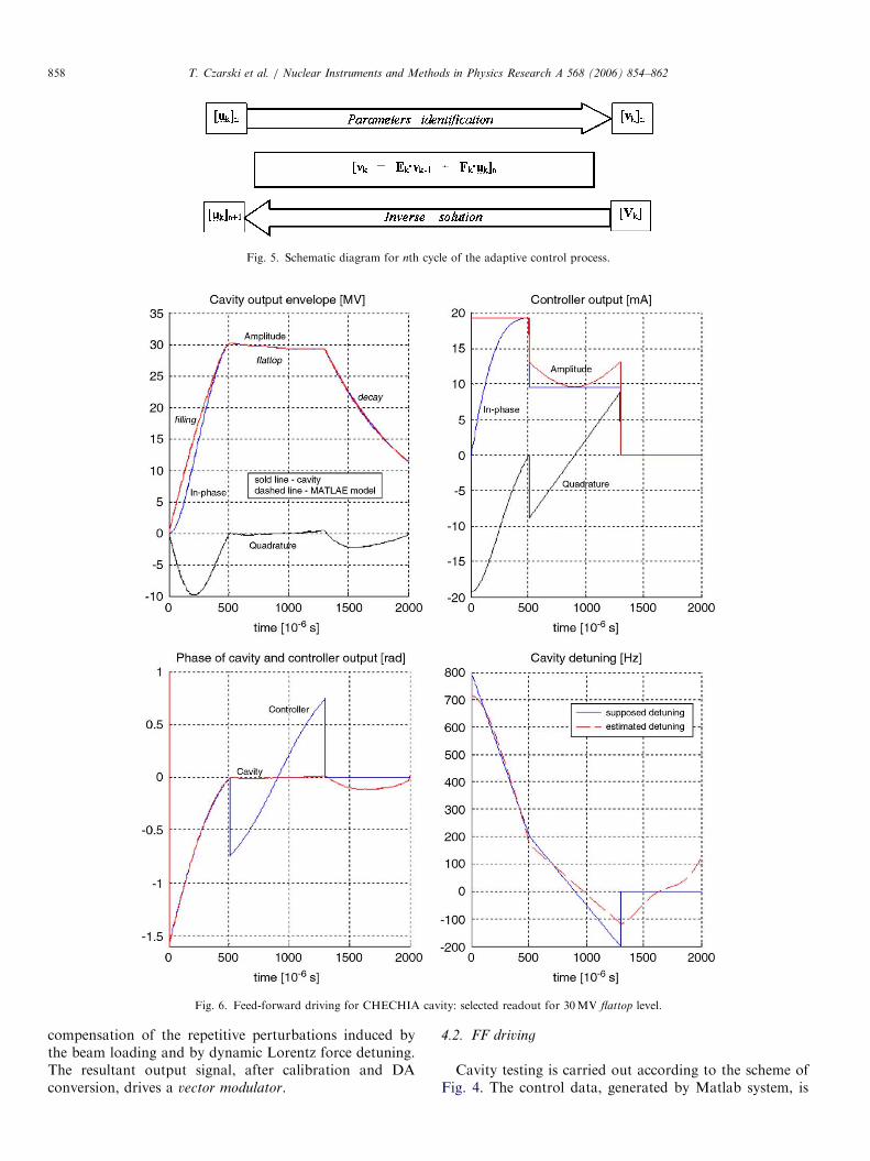
Fig. 5. Schematic diagram for nth cycle of the adaptive control process.

Fig. 6. Feed-forward driving for CHECHIA cavity: selected readout for 30MV flattop level.

T. Czarski et al. / Nuclear Instruments and Methods in Physics Research A 568 (2006) 854–862858

compensation of the repetitive perturbations induced bythe beam loading and by dynamic Lorentz force detuning.The resultant output signal, after calibration and DAconversion, drives a vector modulator.

4.2. FF driving

Cavity testing is carried out according to the scheme ofFig. 4. The control data, generated by Matlab system, is

ARTICLE IN PRESST. Czarski et al. / Nuclear Instruments and Methods in Physics Research A 568 (2006) 854–862 859

loaded to the part of internal FPGA memory as a FF tabledriving the cavity. Input and output data of the cavity isacquired to another area of the memory during a pulse

Fig. 7. Feed forward with feedback driving (gain ¼ 100) for C

Table 2

Analytical solution for two control modes and two ranges of cavity

operation

Range Mode

Feed-forward Set-point

Filling uk ¼ U exp(ijk)/Fk Vk ¼ Vk exp(ijk)

U ¼ 2VTo1/2 Vk ¼ 2V(1�exp(�o1/2kT))

jk ¼ jk�1+TDok jk ¼ jk�1+TDok

Flattop uk ¼ V � (o1/2—iDok) �T/Fk Vk ¼ V ¼ V exp(iF)

operation of the controller. The input vector [uk]n andoutput vector [vk]n for nth pulse are conveyed to Matlabsystem for the parameter identification processing betweenpulses. For comparison purpose, Matlab cavity model isdriven in the same condition according to the estimatedparameters.The required cavity performance can be achieved

iteratively, applying the estimated cavity parameters, togenerate an improved FF table for a next pulse (Fig. 5).Cavity system is characterized by the vectors [Fk]n and[Ek]n, which are time varying within nth cycle. Input vector[uk]n and output vector [vk]n are considered for theparameters estimation in the nth cycle. Input vector[uk]n+1, for a next cycle, is estimated as an inverse solution

HECHIA cavity: selected readout for 25MV flattop level.

ARTICLE IN PRESS

Fig. 8. Diagram of data and operator connections between three

laboratories for A0 control.

Fig. 9. FPGA board embedded on a VME interface carrier board.

T. Czarski et al. / Nuclear Instruments and Methods in Physics Research A 568 (2006) 854–862860

of the system equation, with the required output vector[Vk]. This iterative processing quickly converges to thedesired state of the cavity, assuming repeatable conditionsfor successive pulses.

During flattop operation, the required output phasorVk ¼ V ¼ V exp(iF) is stable and inverse solution of Eq. (3)for a steady state, without a beam, is as follows:

uk ¼ V � o1=2 � iDok

� �� T=Fk (10)

During filling time, the input phasor uk ¼ U exp(ifk)/Fk isestimated in order to drive the cavity with stable forwardpower in the resonance condition, so the required constantamplitude equals U ¼ 2VTo1/2, and time varying phaseequals jk ¼ jk�1+TDok.

Cavity control was performed for different flattop levelsof the field in the range of gradients V ¼ 10–30MV/m withthe phase F ¼ 0. Due to circuit nonlinearities, thecalibration procedure was accomplished for each flattop

level.The results of experiments are presented in Fig. 6 for

CHECHIA cavity setup with flattop level of 30MV/m. Thecavity has been driven with an initial FF table to achieverequired performance: driving on resonance during filling

and field stabilization during flattop range. Supposed cavitydetuning (taken arbitrary) determines the FF table. Thebroken line, with different slopes for filling and flattop, wastaken as supposed cavity detuning curve for the controlpurpose. Additionally, the master oscillator frequency hasbeen tuned to supposed cavity detuning, to optimize theklystron power distribution during flattop level. Theexperiment tries to verify Matlab cavity model andreliability of the identification algorithm. The cavityand Matlab model responses are compared, when drivenin the same condition. A quite good agreement for thecavity and Matlab model is observed, and the two curves ofenvelope are hardly distinguishable in that scale. Therefore,Matlab model of the cavity was confirmed and cavityparameters identification was verified for the controlapplication.

4.3. FF with feedback driving

Required data for set point table are chosen, accordingto the electrical model of cavity (1), for supposed values ofthe cavity parameters. During flattop operation, thecomplex envelope equals V ¼ V exp(iF) and is stable forset point table. During filling time, the required outputphasor Vk ¼ Vk exp(ijk) is estimated for set point table inorder to drive the cavity with stable forward power in theresonance condition, so the amplitude equals Vk ¼

2V (1�exp(�o1/2kT)) and time-varying phase equalsjk ¼ jk�1+TDok.

Table 2 combines analytical solutions for two controlmodes and two ranges of the cavity operation.

Test of the FF cavity driving was repeated and feedbackloop was closed, starting with a small value of the loopgain. No filter was applied. The loop gain was gradually

increased to the possible maximum value for a stablecondition. Loop gains of �250 and �150 were achieved forflattop cavity gradient of 10 and 20MV, respectively, forCHECHIA cavity Fig. 7. The results of experiments forCHECHIA cavity setup, with the flattop level of 25MVand loop gain of 100 are presented in Fig. 11.

ARTICLE IN PRESS

Fig. 10. Software configuration with SIMCON and SUN controller.

Fig. 11. SIMCON control panels for SUN controller at FNAL hardware test.

T. Czarski et al. / Nuclear Instruments and Methods in Physics Research A 568 (2006) 854–862 861

5. Hardware and software setup

SIMCON 2.1 board (cavity SIMulator and CONtroller)was used as FPGA based hardware layer of the controlsystem (Fig. 8). The setup performs fast DSP algorithmsapplying computation of 18 bit resolution.

Experiment with FNPL module in the A0 laboratory atFNAL was done with cooperation of three laboratories:FNAL, DESY and WUT-ISE. DESY and WUT-ISEcommunicated with FNAL using RealVNC program(Fig. 9). All the software ran on a SUN machine installedin a VME crate located at FNAL.

Matlab software was used to control the hardware. Adiagram of software configuration is presented in Fig. 10.

Direct access to FPGA memory is carried out by MEX-functions in Matlab and they are basis for all other m files[5]. Configuration files are used to perform the basic

operations on sets of FPGA registers. Algorithm filesanalyze received data and generate the control tables forFPGA controller. All Matlab functions are available viathe control panel of graphical user interfaces (GUI)(Fig. 11).

6. Conclusion

Preliminary application tests of FPGA controller havebeen carried out using the superconducting cavity inCHECHIA setup. The cavity was driven with FF andfeedback modes. Analogous experiments have been re-peated on ACC1 module of the VUV-FEL (FLASH) andthe remotely controlled FNPL photoinjector cavity moduleat FERMILAB. The calibration procedure is presented.Parameter identification algorithm was incorporated intothe control system development. An over-determined

ARTICLE IN PRESST. Czarski et al. / Nuclear Instruments and Methods in Physics Research A 568 (2006) 854–862862

matrix equation, for the input–output relation, is appliedwith the least-squares solution, for unknown parameters.Polynomial approximation or cubic B-spline functions wasemployed in the estimation of time varying parameters.Electrical model of the cavity has been confirmed andalgorithm of the cavity parameters identification has beenverified for control purpose.

Acknowledgments

The authors would like to thank DESY Directorate forproviding excellent conditions to perform the workdescribed in this paper.

We acknowledge the support of the European Commu-nity Research Infrastructure Activity under the FP6

‘‘Structuring the European Research Area’’ program(CARE, Contract number RII3-CT-2003-506395).

References

[1] T. Schilcher, Vector sum control of pulsed accelerating fields in

Lorentz force detuned superconducting cavities, Ph.D. Thesis, Ham-

burg, 1998.

[2] M. Huning, S.N. Simrock, System identification for the digital RF

control system at the TESLA test facility, in: Proceedings of EPAC98,

Stockholm, 1998.

[3] T. Czarski, R.S. Romaniuk, K.T. Pozniak, S. Simrock, Nucl. Instr.

and Meth. A 556 (2) (2006) 565.

[4] T. Czarski, R.S. Romaniuk, K.T. Pozniak, S. Simrock, Nucl. Instr.

and Meth. A 548(3) (2005) 283.

[5] W. Koprek, P. Kaleta, J. Szewinski, K.T. Pozniak, T. Czarski, R.S.

Romaniuk, Software layer for FPGA-based TESLA cavity control

system (Part I)—TESLA Technical Note, 2004-10, DESY, Hamburg.