Super-Resolution Microscopy: Interference and Pattern Techniques

345

9Super-Resolution Microscopy: Interference and PatternTechniquesGerrit Best, Roman Amberger, and Christoph Cremer

9.1Introduction

In many scientific fields such as biology, medicine, and material sciences,microscopy has become a major analytical tool. Electron microscopy (EM) withnanometer resolution, on the one hand, and light microscopy with a broad appli-cability, on the other hand, allowed for groundbreaking scientific achievements.Even though EM delivers unmatched resolution, light microscopy has never lostits relevance. Because of the vast propagation of fluorescent labeling techniques inrecent years, the method of fluorescence microscopy has actually become one ofthe most important imaging techniques in the life sciences.

However, the intrinsically limited resolution of standard fluorescence microscopycompared to nonlight-optical methods is still a major drawback as many biologicalspecimens are of a size in the nanometer to micrometer range. Therefore, thestandard light-microscopic resolution defined by Rayleigh (1896) (Chapter 2) isoften not sufficient to resolve the objects of interest.

Over last years, different techniques denoted as super-resolution fluorescencemicroscopy have been established to compensate for the deficiency of low spatialresolution. These approaches use fluorescence excitation because this circumstanceallows – in combination with other techniques – access to high-resolution objectinformation.

These super-resolution methods (i.e., 4Pi (Cremer and Cremer, 1978; Hell andStelzer, 1992; Hell et al., 1994; Hanninen et al., 1995 stimulated emission depletion(STED) (Chapter 10), SIM/PEM (Gustafsson, 2000; Heintzmann and Cremer,1999), and localization methods (Chapter 8)) seemingly break the conventionalresolution limit. However, it should be noted that the fundamental resolution limitis not broken directly. The super-resolution methods are based on conditions dif-fering from the assumptions of Rayleigh. Rayleigh’s conclusions for self-luminous(i.e., fluorescent) objects do not consider spatial or temporal variations of the lightintensity. Basically, all super-resolution techniques depend on juggling with thefluorescence excitation or emission.

Fluorescence Microscopy: From Principles to Biological Applications, First Edition. Edited by Ulrich Kubitscheck. 2013 Wiley-VCH Verlag GmbH & Co. KGaA. Published 2013 by Wiley-VCH Verlag GmbH & Co. KGaA.

346 9 Super-Resolution Microscopy: Interference and Pattern Techniques

In this chapter, we describe two wide-field methods that apply interference ofthe excitation light to make high-resolution object information accessible in detail.These are the method of structured illumination microscopy (SIM) (also referredto as patterned excitation microscopy, PEM) and the method of spatially modulatedillumination (SMI).

9.1.1Review: The Resolution Limit

Regarding imaging systems, it is obvious that the rendering power (i.e., thecapability to transmit structural information) is always limited to some degree.To describe the rendering power of an imaging system, the term resolution isemployed. However, the term resolution is ambiguously used and there existdifferent scientific definitions for the resolution power of a system.

A commonly used resolution measure is the definition provided by Lord Rayleigh,which is described in Chapter 2. Rayleigh’s definition is based on the point spreadfunction (PSF) of an optical system (Section 2.3.3).

The PSF or Airy function resembles the image of an ideal pointlike object. TheRayleigh distance defining the resolution is the distance between the maximumand the closest zero point of the PSF.

It is given by

dRayleigh = 0.61λ

n sin α(9.1)

In Chapter 2, the optical transfer function (OTF) is introduced. The OTF is theFourier transform F of the PSF.

F[PSF

(x, y

)] = OTF(

kx, ky

)(9.2)

When the PSF is the same for every position in the object plane, every point ofthe object is broadened by the same PSF. Therefore, the imaging process can berepresented by a convolution:

A′ (x, y) = A

(x, y

) ⊗ PSF(x, y

)(9.3)

Here, A′(x,y) is the image and A(x,y) is the object. The convolution theorem statesthat convolution in position space corresponds to multiplication in frequency spaceand vice versa. Hence, the imaging process can be described in Fourier space by

F[A′] = F [A] × OTF (9.4)

The PSF is band limited, which means that the OTF is zero for high frequenciesbeyond a cut-off frequency kcut-off:

OTF (k) = 0 for |k| ≥ kcut-off (9.5)

All object information beyond this cut-off frequency is filtered out by the OTF andis therefore missing in the image. The lack of high frequencies in the image is thereason for the limited resolution. In Figure 9.1, the cut-off frequency is shown inthree dimensions (3D).

9.2 Structured Illumination Microscopy (SIM) 347

0

0

0

kx

kykz

Figure 9.1 Cut-off frequency of an OTF. The supported frequency region of a conventionalmicroscope is a toroid. For small kx and ky lateral frequency components, the axial compo-nent kz of the cut-off frequency approaches zero (missing cone).

The cut-off frequency can be used as a measure for the resolution of an opticalsystem, as an alternative to the Rayleigh definition.

A resolution definition referring to the object’s frequency is the Abbe definition(Abbe, 1873) of resolution. Abbe considered a fine grating placed on a microscope.The finest, yet resolvable, pattern (with grating distance dAbbe) would define theresolution of the microscope. The calculation yields

dAbbe = λ

2n sin α(9.6)

The corresponding maximum transmittable frequency (i.e., cut-off frequency) isgiven by kcut-off = 2π/dAbbe.

In our case, both definitions dRayleigh and dAbbe are proportional and yield to similarvalues. In the following paragraphs, ways to circumvent this resolution limit arediscussed, which are based on a manipulation of the illumination conditions.

9.2Structured Illumination Microscopy (SIM)

In SIM, the object is illuminated with a periodic illumination pattern.This periodic excitation pattern is used in order to manipulate the object’s spatial

frequencies (Heintzmann and Cremer, 1999; Gustafsson, 2000) as described in thefollowing sections. In SIM, the pattern is projected through the (single) objectivelens and no additional devices or mechanisms are used to illuminate the objectfrom the opposite side.

From another point of view, it can be said that the pattern is generated by aninterference of a number of coherent beams proceeding from the objective lens,meeting in the object plane (Figure 9.2).


Object plane

Z

(c)

(a) (b)

Int. Int.

(d)

X

xx

yy

Objective lens

Back focal plane

Coherent beams

Two-beam-illumination Three-beam-illumination

Figure 9.2 Illumination path in structured illumination microscopy. For the illuminationwith two coherent beams (setup c), the spatial modulation of the illumination intensity (a)is one dimensional (x-direction). In the case of an interference of three beams (setup d),the modulation is two dimensional (x- and z-directions) (b).

The periodic pattern can be of arbitrary shape, but typically the modulation ofthe pattern is only one dimensional in the focal plane(x − y-plane) as is the casewith the patterns shown in Figure 9.2. Two methods to spatially modulate theexcitation intensity in SIM are common: two-beam interference (also denoted byfringe projection) and three-beam interference (grid projection). Examples for opticalsetups generating the coherent beams are given in Section 9.2.6.

In the three-beam interference case, one light beam propagates along the opticalaxis and two beams span an angle with the first beam. One of the other beamspropagates at an angle α to the optical axis and the other one at the angle −α.All three beams span a common plane (interferometer plane). The resultinginterference pattern has a modulation along one direction in the focal plane andalso a modulation along the optical axis.


The other method works with only two beams and corresponds to the three-beam case with a blocked central beam along the optical axis. The correspondinginterference pattern exhibits only a modulation along the focal plane (x − y-plane).

In the following, the image formation process and, thus, the resolution im-proving effect of SIM will be shown using the more simple method of two-beaminterference.

9.2.1Image Generation in Structured Illumination Microscopy

In this section, a mathematical description of the image generation process in SIMis developed.

As mentioned in Section 9.1.1 and in Chapter 2, the imaging process of awide-field microscope can be described by

A′ (x, y) = A

(x, y

) ⊗ PSF(x, y

)(9.7)

where A′ is the image and A the object. The PSF is the impulse response blurringthe image. The object A is the fluorescence light distribution in the object plane.

When fluorescence saturation is insignificant (under usual fluorescencemicroscopy conditions), the object distribution is proportional to illuminationintensity Iill(x,y) and fluorophore distribution ρ(x,y):

A(x, y

) = ρ(x, y

) × Iill

(x, y

)(9.8)

In conventional wide-field microscopy, the Illumination intensity is constant andthe object is essentially the fluorophore density.

In SIM, however, the illumination is spatially variant and this variation is carriedthrough into the image. For the case of two-beam illumination (Figure 9.2a), theillumination distribution is given by

Iill

(x, y

) = I0

[1 + m cos

(kGxx + kGyy + ϕ

)](9.9)

or

Iill (r) = I0

[1 + m cos

(kGr + ϕ

)](9.10)

in vector notation with the position vector r.The modulation strength m is a scalar value between 0 and 1. For m = 1,

the distribution has a minimum of zero and a maximum of 2I0. The intensitymodulation takes place in the x − y-plane. To express the modulation in the 2Dspace, the k-vector of the grating kG with |kG| = 2π/GSIM is used, where the gratingconstant GSIM is the period of the modulation. kG points in the direction of themodulation (i.e., it is perpendicular to the stripes of the pattern and pointing alongthe object plane (x − y-plane)).The lateral position of the illumination pattern isdetermined by the phase ϕ.

Substituting Eq. (9.8) in Eq. (9.7) yields

A′ (r) = [ρ (r) × Iill (r)

] ⊗ PSF (r) (9.11)


Now, the image information in Fourier space is given by

A′ = FT

[A′] = FT

[ρ × Iill

] × OTF (9.12)

The multiplication of ρ and Iill transforms into a convolution because of theconvolution theorem:

A′ = ρ ⊗ Iill × OTF (9.13)

The Fourier transform of the illumination pattern (Eq. (9.9)) is

Iill (k) = 1

2π× I0

[1 + m cos

(kGr + ϕ

)]e−i(kr) dr (9.14)

Using the identity

cos x = 1

2

(eix + e−ix) (9.15)

FT(Iill) becomes

Iill (k) = 1

2π×I0

(1 + m

2ei(kGr+ϕ) + m

2e−i(kGr+ϕ)

)e−i(k×r) dr (9.16)

Expanding this equation yields

Iill (k) = 1

2π×I0

(e−ikx + m

2e−i(kx−kGx)eiϕ − m

2e−i(kx+kGx)e−iϕ

)dr (9.17)

With the Dirac delta distribution in exponential form

δ(k − α

) = 1

2π×ei(xk+xα) dx (9.18)

the Fourier transform of the illumination pattern becomes a sum of delta functionswith complex prefactors depending on ϕ:

Iill (k) = 2π × I0 ×[δ (k) + m

2eiϕδ

(k − kG

) + m

2e−iϕδ

(k + kG

)](9.19)

One delta function is located at the origin and two at the reciprocal period of theillumination pattern.

In the Fourier-transformed image A′, the convolution of these delta functionswith the Fourier-transformed object distribution leads to a sum of copies of theobject information shifted by the positions of the delta functions. Each copy ismultiplied by its corresponding complex coefficient:

A′(k) = OTF (k) × I0

1√2π

×[(

ρ (k) + m

2eiϕρ

(k − kG

) + m

2e−iϕρ(k + kG

)](9.20)

How far the single additional copies are shifted in Fourier space is defined by theangle α and the wave vector k of the incident light waves.

Note the low-pass filter property of the OTF (during image formation, the OTFis multiplied by FT[ρ × Iill]). As the frequencies of the additional copies of theimage are shifted, a frequency region of previously irresolvable frequencies beyondthe cut-off limit kcut-off of these copies is shifted into the area of frequencies that


are transmitted by the OTF. This frequency information is superposed with theinformation of the other copies and located in the frequency region imaged by themicroscope. Therefore, it has to be separated and shifted back to its appropriateposition after image acquisition. The separation and reconstruction process will bediscussed in Section 9.2.2.

When it is possible to separate the shifted information in the acquired image, theinformation can be shifted back to its original position. It is apparent that now thefrequency region of the image spans further in the direction of the modulation ofthe illumination pattern compared to the original image. Therefore, the resolutionhas been enhanced by this process as higher frequency information is transmittedinto the image. The factor of resolution improvement is given by the factor bywhich the size of the frequency region of the image is expanded.

The size of the resulting frequency region depends on the grating distance of theillumination pattern. To calculate the maximum possible resolution improvementby SIM, the minimum possible grating distance has to be taken into account.It is reached when the two incident coherent excitation beams with the vacuumwavelength λ0ex span the maximum angle. Therefore, the minimum gratingdistance is given by

GSIMmin = λ0ex

2n sin(αmax

) = λ0ex

2NA= dAbbe (9.21)

which is the Abbe definition for the minimum grating distance of a yet resolvablegrating in the object plane (for transmitted light microscopy).

In fluorescence microscopy, the wavelength of the emission light is close tothat of the excitation light (λem ≈ λex). Hence, the reciprocal grating period of thesmallest possible illumination pattern approximates the cut-off frequency kcut-off.The delta functions of the Fourier-transformed illumination pattern are locatedat the positions −2π/GSIM and +2π/GSIM. Therefore, the origins of the copies ofFourier-transformed information are shifted to the cut-off limit (Figure 9.3b). Whenthese copies are separated and shifted back, the region of accessible informationin Fourier space is twice as large as in the standard microscopy case. Thus, theresolution improvement in linear SIM can reach a factor of 2.

The term linear is used because in this case, the dependency of the fluorescenceemission intensity is considered to be linear to the excitation intensity.

This assumption is true only for low-illumination conditions, where satura-tion and photobleaching effects can be neglected (which is the case under usualmicroscopy conditions). Saturation and photobleaching effects result in a decreas-ing gradient of the emission response with increasing excitation intensity. It hasbeen shown (Heintzmann, Jovin, and Cremer, 2002; Gustafsson, 2005) that thisnonlinear effect can be used to increase the resolution of SIM beyond the factorof 2 when the magnitude of the nonlinearity is maximized by the applicationof appropriate setup conditions (e.g., special fluorochromes, matched excitationintensities). In this case, the effective fluorescence pattern that is multiplied withthe fluorochrome distribution contains the periodic illumination intensity patternand additionally higher harmonics of the fundamental pattern. In Fourier space,


Position space Frequency space

(a) (b) (c) (d)

Figure 9.3 Accessible frequency region bySIM. The illumination pattern (a) containsthree delta peaks in frequency space asillustrated in the Fourier-transformed rawimage (b). The bold outline demonstratesthe frequency limit. The raw data (b) con-sists of superposed original image infor-mation positioned at three different ori-gins. After separation, the information can

be shifted back to its respective position,resulting in an expanded accessible fre-quency area (c). To expand the resolutionin the object plane isotropically, the illu-mination pattern is rotated to conduct theimage acquisition with several illuminationpattern orientations (d). (Source: Reprintedfrom Best et al., 2011, with permission fromElsevier.)

the higher harmonics shift the image information by the double, triple, or moreamount of the shift by the fundamental pattern.

The twofold resolution improvement in linear SIM yields a lateral resolutionof ∼100 nm (Heintzmann and Ficz, 2007), whereas wide-field- and confocalmicroscopy achieve ∼230 and ∼180 nm lateral resolution, respectively (Pawley,2006).

However, when an illumination pattern with modulation in only one directionin the optical plane (i.e., the plane of focus) is used, the resolution improvement isanisotropic and only maximal in the direction of the modulation (Figure 9.3c). Toattain a more isotropic resolution, the direction of the modulation has to be appliedin several directions in the optical plane (Figure 9.3d).

An alternative, depictive approach to understand the resolution enhancing effectprovided by SIM is to consider the Moire effect, as shown in Figure 9.4. When twofine gratings are superposed, a third raw grating with a spatial period (or gratingdistance) G3 occurs. If one of the fine original patterns with a spatial period G1 isknown and also the resulting pattern is known, while the second fine grating withG2 is unknown, the unknown pattern can be reconstructed mathematically.

The known and the unknown fine grating represent the SIM excitation patternand the high-frequency object information, respectively, whereas the raw gratingrepresents the detected image.

9.2.2Extracting the High-Resolution Information

When structured illumination is applied, the total spatial frequency informationtransmitted through the objective lens is increased. However, the additionalinformation is overlaid with the original image information, as described inSection 9.2.1.


Figure 9.4 Moire effect. If two fine patterns are superposed, a third, raw pattern canoccur. (Source: Reprinted from Ach et al., 2010, with kind permission from SpringerScience+Business Media.)

The additional information, therefore, has to be separated and shifted to thecorrect position in Fourier space. To separate the components, the acquisition ofseveral images with different positions of the illumination pattern is required. Bythis method, the complex coefficients (1, (m/2)eiϕ , and (m/2)e− iϕ) of the imagecopies depending on the grating position ϕ (see Eq. (9.20)) can be calculated forthe different grating positions consecutively. The image information belonging tothe single copies can be separated afterward by the respective coefficient. Whenusing two-beam interference, three images with different grating positions aresufficient to solve the equations; for three-beam interference, five images arenecessary.

After separation, the copies of the image information can be shifted to theircorrect position by the reciprocal vectors of the illumination grating. When thecorrectly processed information of the different copies is added, the resulting imagehas a higher resolution than the original image.

As described above, the resolution improvement in the focal plane is anisotropicif the modulation of the illumination pattern is one dimensional in the lateraldirection.

In order to achieve an almost isotropic resolution improvement nonetheless inthis case, image series are taken at different angles of the periodic illuminationpattern (typically at 0◦, 60◦, and 120◦ or at 0◦, 45◦, 90◦, and 135◦; Figure 9.3d).

It is also mathematically possible to use a two-dimensional grating (e.g., ahexagonal pattern) to generate the diffraction orders of the excitation light.

9.2.3Optical Sectioning by SIM

Not only the lateral resolution as shown in the two-dimensional example in theparagraph above, is improved in SIM compared to standard wide-field microscopy


but also the confocality is improved, resulting in an optical section with less signalfrom the out-of-focus region.

This effect becomes clear when the wide-field OTF (Figure 9.1) is considered. Forthe spatial frequencies kx, ky = 0, and kz �= 0, the OTF is always zero. A cone-shapedfrequency region along the optical axis frequencies kz in the OTF is missing. Thecorresponding information is not transmitted by the microscope. This ‘‘missingcone’’ problem results in the fact that conventional microscopy suffers from a poorz-resolution.

As shown in Figure 9.5, the additional object information copies provided by SIMare capable of covering the missing cone of the original OTF and therefore yield animproved optical sectioning power of SIM compared to conventional fluorescencemicroscopy. However, in the case of two-beam illumination (Figures 9.2a,c, and9.5a,c), confocality is improved only if the illumination pattern frequency is (slightly)smaller than the cut-off frequency. At the cut-off, the missing cones overlap andtherefore remain uncovered.

As is the case with lateral resolution, it is difficult to quantify the axial resolutionof a microscope and it is important to find a suitable model to calculate or measurecomparable quantitative values for different microscopy methods. For example,the full width at half maximum (FWHM) of the 3D PSF in the axial dimensioncould be used. However, this z-direction FWHM depends on the x and y positions(Figure 2.12).

In the work of Karadaglic and Wilson (2008), the optical sectioning powers of twodifferent SIM setups and of a confocal microscope were compared using a modelof a thin fluorescent sheet located in the focal plane. The ability to determine thez-position of the sheet by the microscopes was compared.

It was shown that both two-beam interference (fringe projection) and three-beaminterference (grid projection) SIM exhibit optical sectioning strengths comparableto that of a confocal microscope. However, three-beam interference providedbetter results in terms of confocality compared to two-beam interference. On theother hand, two-beam interference requires less single images at different phase

(a)

(c) (d)

(b)kz

kx

Figure 9.5 Resulting OTF in two- (a,c) andthree-beam illumination (b,d). The blackspots in the microscope’s wide-field OTFs(a: two-beam and b: three-beam) show theorigins of the shifted object informationcopies. When these copies are shifted back

(c,d) to their correct positions, the effec-tive OTF increases in size. The black outlineshows the original wide-field OTF cut-off bor-der. The borders of the shifted OTFs areshown in gray. The corresponding illumina-tion patterns are shown in Figure 9.2a,b.


positions (3 instead of 5) for reconstruction, and because less object informationcopies are used, it is less susceptible to noise in the raw data.

The answer to the question whether two- or three-beam illumination is ultimatelymore favorable depends on the specimen that is analyzed.

9.2.4How the Illumination Pattern is Generated

For structured illumination, a multitude of coherent light beams is necessary togenerate the illumination conditions shown in Figure 9.2.

Basically, two techniques have been developed to arrange this: the application ofa diffraction grating (Figure 9.6a) and the use of an interferometer (Figure 9.6b).In Section 9.2.6, examples for both ways are shown.

The two techniques differ in the dependence between the period of the illumina-tion pattern and the wavelength of the excitation light (Figure 9.6).

In setups applying a diffraction grating in a conjugate image plane, there isan imaging condition: an image of the grating is projected into the object plane.Therefore, the spatial period of the illumination pattern is independent from theillumination light’s wavelength. Hence, the illumination light must not be coherent.An inherently incoherent light source (e.g., gas-discharge lamp or light-emittingdiode (LED)) can be used instead of a laser.

For an interferometer setup, on the other hand, the illumination pattern hasa period proportional to the wavelength of light. The larger the wavelength, thecoarser the pattern becomes. Here, the light source has to be coherent in order toachieve a periodic intensity pattern (Figure 9.6b). For interferometer setups, theangle of the excitation light beams depends only on the angle of the interferometer.If this angle is set to a suitable value according to the objective lens’ numericalaperture (NA) once, a change in interference angle is not necessary for differentwavelengths. For diffraction grating setups, a change in grating might be necessaryif the wavelength is changed. As shown in Figure 9.6a, the red beams hit theobjective lens at the utmost border, whereas the blue beams are close to the centerof the objective lens.

9.2.5Mathematical Derivation of the Interference Pattern

In the equations for the illumination pattern (Eq. (9.9)) and the derived statements,a variable modulation strength m was used.

To analyze where the modulation strength is originating from, the interferencepattern for a two-beam interference SIM setup is derived. The two initial beamsare considered to be equally strong and have equal linear polarization p0. The rightbeam has a phase shift ϕ compared to the left beam.

In the following, the complex exponential form for the superposing waves isused instead of the trigonometric form. Both beams propagate identically alongthe z-direction before passing the objective lens. While passing the objective, the


(a) (b)

Figure 9.6 Beam path and interference pattern for grating (a) and interferometer setup (b).In the interferometer setup shown here, the zero order of diffraction is blocked as well as 2and −2 orders and higher orders.

left beam is rotated by the angle α and the right beam by −α (Figure 9.7) aroundthe y-axis.

Before passing the lens, the electric fields of the left and the right beam are givenby

El0 = p0E0ei(k0r−ωt) (9.22)

and

Er0 = p0E0ei(k0r−ωt−ϕ) (9.23)


PS(a) (b)

pIpIpr

pr

Figure 9.7 Polarization of the beams before and after passing the objective lens forpolarization perpendicular (s; (a)) and parallel (p; (b)) to the interferometer plane.

The polarization vector is a unity vector (|p0| = 1) pointing in the direction in whichthe electric field oscillates.

The original wave vector k0 points along the z-direction:

k0 =0

01

2π

λ(9.24)

After the lens, the rotated polarizations of the beams are given by

pl = Ry (α) p0 = cos α 0 sin α

0 1 0−sin α 0 cos α

p0 (9.25)

and

pr = Ry (−α) p0 =cos α 0 −sin α

0 1 0sin α 0 cos α

p0 (9.26)

through application of the rotation matrix Ry around the y-axis.The same rotation accounts for the wave vectors, which yields

kl =sin α

0cos α

2π

λ(9.27)

kr =−sin α

0cos α

2π

λ(9.28)

El = plE0ei(klr−ωt) (9.29)

Er = prE0ei(krr−ωt−ϕ) (9.30)

The superposition Es = El + Er in the object plane yields

Es = E0

(ple

i(klr−ωt) + prei(krr−ωt−ϕ)

)(9.31)


The intensity is proportional to the absolute square of the electric field:

I ∝ |Es|2 = > I = a|Es|2 = a EsE∗s (9.32)

with a proportionality constant a. By substituting Eq. (9.31) in Eq. (9.32), theintensity becomes

I = 2aE02 (

1 + plpr cos[(

kl − kr

)r + ϕ

])(9.33)

after some rearrangements. Substituting the wave vectors kl and kr (Eqs (9.27) andEq. (9.28)) yields

I = 2aE02(

1 + plpr cos[

4π sin α

λx + ϕ

])(9.34)

Obviously with plpr = m and 2aE20 = I0, the term is identical to the illumination

pattern of a two-beam interference SIM microscope (Eq. (9.9)).When both interfering beams of a two-beam interference SIM setup are equally

strong, the modulation strength depends on the primary polarization of thebeams and on the angle α by which the beams are deflected by the objective. Toexamine these effects, we compare two extreme cases of linear polarization: po-

larization perpendicular (s)

p0s =0

10

to the interferometer plane and parallel

(p)

p0p =1

00

to the interferometer plane (Figure 9.7). The interferometer

plane is the plane that is spanned by the two beams.If the polarization of the incoming beams is perpendicular (s), the polarization

of the single beams (pl,pr) will not be changed by passing through the objectivelens (application of Ry(α) and Ry(−α)). For beams parallel (p) to the interferometerplane, owing to the change in beam angle, the polarization of the left beam isrotated by α and of the right by −α. For p polarization and α = 45◦, the polarizationsand therefore the electric fields of both beams are perpendicular. The modulationstrength m = plpr becomes zero and the resulting intensity of the object planebecomes constant (Figure 9.8b). Usually, the interferometer plane is rotated todifferent angles (usually 0◦, 60◦, and 120◦) around the optical axis in the SIMimage acquisition process. To achieve a high modulation strength for all angles,the polarization of the excitation light has to be rotated with the pattern to allowfor s-polarization in every case. This can be done, for example, with a rotatablehalf-wave plate or an electro-optic modulator.

9.2.6Examples for SIM Setups

In SIM, the excitation intensity in the focal plane is a periodic pattern. To achievethis illumination distribution, various different setups have been established.Commonly, the excitation light is projected through the same objective lens that


s Polarization, 60°

–5000.0

0.5

1.0

0500x (nm)

p Polarization, 60°

0

0.0

0.5

1.00

500

1000

z (nm)

–500

500x (nm)

p Polarization, 45°

0

0.0

0.5

1.0

Inte

nsity

–500

500x (nm)

s Polarization, 45°

0.0

0.5

1.0

–5000

500x (nm)

(a)

(c)

(b)

(d)

Inte

nsity

Inte

nsity

Inte

nsity

0

500

1000

z (nm)

0

500

1000

z (nm)

0

500

1000

z (nm)

Figure 9.8 (a–d) Intensity distribution in the object plane for perpendicular (s) and parallel(p) polarization at different angles.

is used for the detection of the fluorescence in order to generate a standing wavefield, even though other illumination techniques with the use of additional opticaldevices or even near field excitation are possible.

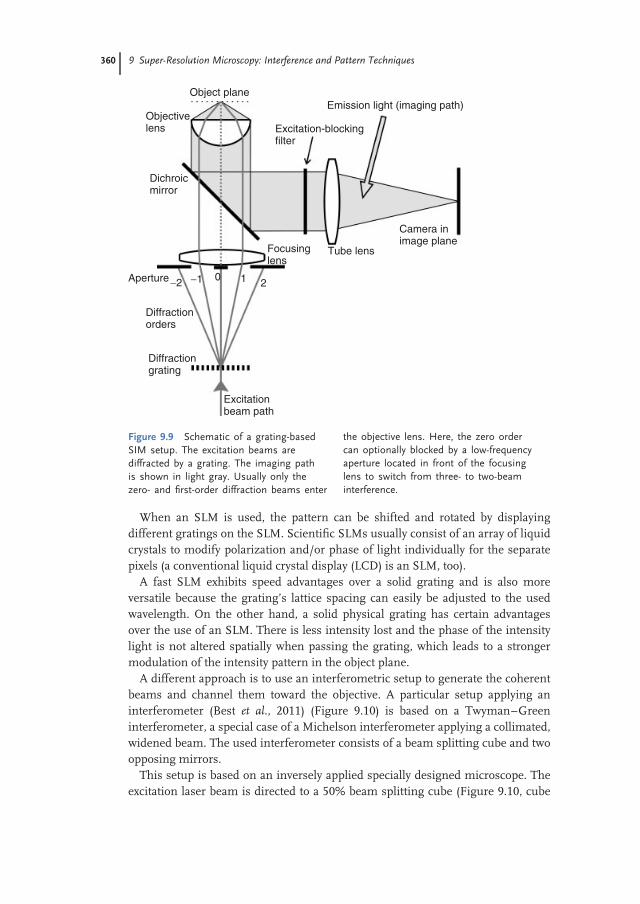
Most commonly, SIM microscopes use either a physical grating (Heintzmannand Cremer, 1999; Gustafsson, 2000) or a synthetic grating generated by a spatiallight modulator (SLM) (Hirvonen et al., 2008; Kner et al., 2009) in an intermediateimage plane to create the modulated pattern in the object plane (Figure 9.9).

When a grating is used, usually the setup is applied in a way that only the zero-and the first-order diffractions of the excitation beams enter the objective lens. Theuse of higher orders (five and more beam interference) is possible but would leadto a more complicated separation of the copies of the Fourier-transformed objectinformation and a lower signal-to-noise-ratio as the number of copies would behigher. The zero-order diffraction (undiffracted beam) can optionally be blocked inorder to apply two-beam interference; the use of zero, plus, and minus first orderleads to the case of three-beam interference.

The phase (i.e., position) of the interference pattern in the object plane canbe shifted by moving the diffraction grating in the intermediate image plane. Tochange the orientation of the pattern’s modulation, the grating can be rotated.

Alternatively, a two-dimensional grating can be applied to generate a patternwith modulation along multiple axis in the object plane, as noted in the previoussection.


Tube lens

210−1−2

Camera inimage plane

Focusinglens

Dichroicmirror

Objectivelens

Object planeEmission light (imaging path)

Excitation-blockingfilter

Aperture

Diffractionorders

Diffractiongrating

Excitationbeam path

Figure 9.9 Schematic of a grating-basedSIM setup. The excitation beams arediffracted by a grating. The imaging pathis shown in light gray. Usually only thezero- and first-order diffraction beams enter

the objective lens. Here, the zero ordercan optionally blocked by a low-frequencyaperture located in front of the focusinglens to switch from three- to two-beaminterference.

When an SLM is used, the pattern can be shifted and rotated by displayingdifferent gratings on the SLM. Scientific SLMs usually consist of an array of liquidcrystals to modify polarization and/or phase of light individually for the separatepixels (a conventional liquid crystal display (LCD) is an SLM, too).

A fast SLM exhibits speed advantages over a solid grating and is also moreversatile because the grating’s lattice spacing can easily be adjusted to the usedwavelength. On the other hand, a solid physical grating has certain advantagesover the use of an SLM. There is less intensity lost and the phase of the intensitylight is not altered spatially when passing the grating, which leads to a strongermodulation of the intensity pattern in the object plane.

A different approach is to use an interferometric setup to generate the coherentbeams and channel them toward the objective. A particular setup applying aninterferometer (Best et al., 2011) (Figure 9.10) is based on a Twyman–Greeninterferometer, a special case of a Michelson interferometer applying a collimated,widened beam. The used interferometer consists of a beam splitting cube and twoopposing mirrors.

This setup is based on an inversely applied specially designed microscope. Theexcitation laser beam is directed to a 50% beam splitting cube (Figure 9.10, cube


Vertical view

Horizontal view

Focusinglens

Web cam

Gray filterC

A B

Beam aperture

Excitation beam

Fluorescence detection beamSpecimen

Objective

Focusing lensDichromatic beam splitter

CCD camera

Objective

Table

MirrorBlocking filter Tube lens

404, 488, 568, 647 nm

90° deflection at dichromatic beam splitterλ/2 platePiezo-adjustable mirrors

Figure 9.10 Interferometer setup for SIM.The schematic is simplified. The excita-tion beams are deflected by 90◦ onto thevertically applied objective by a dichro-matic beam splitter. The deflection is notshown to improve visibility. The detectionpath is shown only in the horizontal view.

The elements dashed are used for theoptional three-beam interference mode.The objects labeled with A, B, and C arebeam splitters. The arrows indicate mov-able elements. (Source: Reprinted fromBest et al., 2011 with permission fromElsevier.)

A), positioned in a focal point of the focusing lens. Half of the beam is reflected by90◦ as the other half passes through the cube without a change in direction. Theresulting two beams are then reflected with mirrors by 180◦ back into the cube.After the light passes the beam splitter, again, two beams, each at 1/4 intensity, aregenerated, which leave the cube channeled toward the focusing lens. If the beamsplitting cube is rotated around the axis perpendicular to the table by an angle θ ,one beam is deflected by 2θ , as the other beam is deflected by −2θ . Thus, theinterference pattern can be adjusted by rotating the beam splitter. The beams passthe focusing lens and are then deflected by a dichromatic beam splitter toward theobjective. After passing focusing lens and objective, the interference of the twobeams in the object plane leads to a sinusoidal pattern with modulation parallelto the object plane. The orientation of the modulation can be changed by rotatingthe beam splitter around an axis parallel to the ground and perpendicular to theprevious rotation axis. It is therefore possible to generate sinusoidal interferencewith arbitrary period and direction, which makes it possible to adjust the periodof the pattern in accordance to the particular task and wavelength. A webcam canbe used to monitor the interference pattern directly. The microscope also offersthe option to use a third beam, not deflected by an angle and positioned centralto the two outer deflected beams, in order to generate a three-beam interference


pattern. The beam splitter extracting the central beam (C) is located in the beamline previous to the other splitters. The phase of the pattern can be altered byshifting the relative phases of the separate beams. To accomplish this accuratelyand quickly, piezo actuators are attached to the mirrors facing the rotatable beamsplitting cube (A).

9.3Spatially Modulated Illumination (SMI) Microscopy

9.3.1Overview

SMI is a microscopy method that can be used for precise size measurements ofsmall fluorescent objects.

In SIM, the excitation light comes from one objective lens and the interferencepattern is spanned along the focal plane (e.g., x − y-plane) whereas in SMImicroscopy, two counterpropagating waves from two opposing objective lenses areused (Figure 9.11). The specimen is located between the two objectives, where thetwo beams form a standing wave pattern. Here, the interference pattern modulatesonly along the optical axis (z-direction).

Because the two beams are counterpropagating, the period of the interferencepattern fringe distance d is very small (i.e., it has a high frequency). Analog tothe case in SIM, the relation that the finer the pattern, the higher the resolutionis valid. When the resulting OTF is considered (Figure 9.12b), as in Figure 9.3and Figure 9.5 for SIM, in the SMI case, copies of the OTF appear shifted far inthe z-direction of spatial frequencies kz. The OTF copies have no overlap with thewide-field OTF in the center, which means that the supported frequency region ofthe resulting OTF is not continuously interconnected. Even though information

Backfocalplane Objective Objective

λ/2n

d = λ/2n cosθ

Opticalaxis

x

y zθ

Figure 9.11 SMI setup. Two coherent light beams propagate through two opposing objec-tives and interfere in to object plane with a fringe distance d.

9.3 Spatially Modulated Illumination (SMI) Microscopy 363

5050

50

100100

100

150150

150

200200

200

Position x (10 nm)Position y (10 nm)

Pos

ition

z (1

0 nm

)

kz

kx

(a) (b)

Figure 9.12 Simulated SMI-PSF (a) and corresponding OTF (b). While in structured illumi-nation microscopy (SIM) the intensity is usually modulated along the optical plane, in SMIthe intensity is typically modulated along the axial direction.

of very high-resolution frequencies in the axial direction (dashed structures inFigure 9.12b) is transmitted by the microscope, information from large frequencyregions in between is not accessible.

As a consequence, the generation of high-resolution images free of artifacts asdone by SIM is not possible by this method because large fractions of the object’smoderately high-resolution information get lost.

Therefore, a priori knowledge concerning the analyzed specimen is necessary inorder to use SMI microscopy. However size and position measurements of smallobjects can be done with a precision far beyond the diffraction limit (typically 40nm) with this method.

9.3.2SMI Setup

A typical SMI setup is shown in Figure 9.13. In order to generate two coherentand collimated beams, a collimated laser beam is split using a beam splitter. Eachbeam passes an additional lens for each objective, where the focal plane of the lensis located in the back focal plane of the objective. This converts the objective andthe focusing lens into a collimator. With this optical setup, an interference patternof sinusoidal shape along the optical axis can be generated between the objectivelenses. The sample is placed between the objective lenses and can be moved alongthe optical axis through the interference pattern. The detection, which is equal toconventional wide-field fluorescence detection, is realized by only one objectivelens, which is used in conjunction with a dichroic mirror to separate the excitationlight from the fluorescence signal. During image acquisition the object is movedin precise axial steps (e.g., each 20 or 30 nm) through the standing wave field. Ateach step, a fluorescence image is registered.


Lasers

488 647 568

DM2

DM3

L1

L2

DM1 M1

M2,M3

M4

B1

B2

M5

M6

OL2

L3

BS

BF2

Led

OL1 DM4

L5

BF1 CCD

L4

M7

PZ1

Slide

Figure 9.13 Horizontal SMI setup with three different laser sources, one LED for com-mon transmitted light illumination and one monochrome charge-coupled device (CCD)camera. (Source: Reprinted from Reymann, 2008, with kind permission from SpringerScience+Business Media.)

9.3.3The Optical Path

The fringe period of the standing wave located in the object plane depends on theexcitation wavelength λ, the refractive index n of sample, and slide, as well as apossible tilting angle θ of the beams relative to the optical axis (Figure 9.11).

In the following the mathematical expression for the intensity distribution isderived.

Two counterpropagating coherent electromagnetic waves El and Er interfere inthe focal region. It is assumed that both beams have the same amplitude A and thatboth beams might be rotated around the y-axis by an angle ϑ . The beam passingthrough the right objective (Figure 9.13) has a phase delay relative to the left beamof ϕ. The result is a periodic standing wave field Es with an intensity distribution Is.

The calculation of the intensity distribution of the SMI interference patterncan be derived from the equation for the pattern of a two-beam interference


SIM (Eq. (9.33)):

I = I0

(1 + plpr cos

[(kl − kr

)r + ϕ

])(9.35)

In the SMI case (Figure 9.11), the wave vectors of the two beams are given by

kl =sin ϑ

0cos ϑ

k (9.36)

kr = sin ϑ

0−cos ϑ

k (9.37)

with the absolute value k of the wave vector k.

k = ∣∣k∣∣ = 2 π

λ(9.38)

The polarization is considered to be parallel to the y-axis (s-polarization):

pl = pr =0

10

(9.39)

The intensity becomes

I = I0

(1 + cos [2 cos ϑ kz + ϕ]

)(9.40)

The illumination pattern can be phase shifted by changing the optical path length

of the interferometer. k, the norm of the wave vector k, is expanded by the refractiveindex factor n of the media as the wavelength of light is inversely proportional to n:

λ = λ0

n(9.41)

=> k = k0 n; k0 = 2π

λ0(9.42)

The grating distance GSMI of the pattern in z-direction can be derived fromEq. (9.35) by

(kl − kr

) = 0

0GSMI

= 2kGSMI cos ϑ = 2π (9.43)

GSMI = λ0

2n cos ϑ(9.44)

This means that for samples with a thickness larger than GSMI, multiple interferencefringes are located inside this volume and as a result, no unique phase positionmight be distinguishable. Several maxima of the illumination pattern might belocated in the depth of the sample at once independently of the actual phase of thepattern.

For a well-aligned system with a tilting angle below 10◦ (cos ϑ ≈ 1), the cosineterm in Eq. (9.44) can be neglected. A fringe period is obtained that is proportional


to the vacuum wavelength λ0 divided by two times the refractive index. Usingimmersion media with high refractive index, n will be roughly 1.5. In this case,the fringe distance is λ divided by 3. Therefore, an excitation wavelength of 488nm results in a fringe distance of approximately 163 nm. This means that thecos2-intensity profile of the excitation has a maximum every 163 nm. When thisvalue is compared with the axial depth of focus (∼600 nm for an NA 1.4 objectivelens), it can be seen that there is more than one intensity maximum within the focaldepth (Figure 9.12a). Hence, it is possible to achieve information from the high-resolution region beyond the classical resolution limit. The approach is describedin the following sections.

9.3.4Size Estimation with SMI Microscopy

There are two major effects, which occur when moving the sample through thefocus of the detection objective lens. On the one hand, the detected intensityis modulated by the interference of the excitation pattern, while the modulationcontrast depends on the object size. On the other hand, there is a variation ofintensity between objects in the focus and out of the focus.

The analysis of SMI data is primarily based on these two effects. The axial PSF of awide-field microscope is given by a sin c2 function (Chapter 2). As a result of the two-beam interference, the excitation intensity distribution is given by a cos2 function.

When the illumination pattern is kept fixed to the object plane and a pointlike ob-ject is moved along the z-direction, two effects superpose. The illumination intensitywill vary sinusoidally because of the illumination pattern and the image of the objectwill move through the focus. As a result, the illumination pattern and the wide-fieldPSF are multiplied to form the resulting SMI-PSF (Figure 9.14). Figure 9.12 showsthe 3D SMI-PSF on the left and the corresponding OTF on the right.

The axial SMI-PSF shows as envelope the sin c2 function, which is modulated bya cos2 interference pattern. In this example of an infinitely small pointlike object,

FWHMEPI

FWHMf

FWHMSMI

SMI AxialPSF

Epifluorescentintensitydistribution

Figure 9.14 Axial detection PSF (left), excitation pattern (middle), and resulting SMI pointspread function (right).


the modulation contrast R is 1. The modulation contrast R is defined as follows:

R = Imax − Imin

Imax(9.45)

where Imax and Imin represent the maximum and minimum intensity values ofthe inner and outer SMI-PSF envelopes, respectively. In other words, the detectedintensity distribution AID is an overlap of the small fringes from the excitationlight modulation and the envelope function from the axial detection of the objectivelens (Schneider et al., 1999; see also Figure 9.14):

AID =(

sin(k1z

)k1z

)2

× (a1 × cos2 (

k2z) + a2

)(9.46)

In this equation, k1 represents the FWHM of the envelope function, k2 is the wavevector of the standing wave field, a1 represents the modulation strength, and a2

defines the modulation contrast. For simplification, additional phase offset valuesand nonmodulated parameters are neglected in this formula.

When, instead of a hypothetical point-shaped object, a large object is analyzed,the modulation contrast is smaller than 1 and varies with the object’s size andgeometry (Failla et al., 2002; Albrecht et al., 2001; Wagner, Spori, and Cremer,2005). When analyzing biological nanostructures, it is often suitable to assume aspherical geometry. Figure 9.15 shows the modulation contrast R in dependenceof the diameter of a spherical object. Obviously the modulation contrast graph isnot bijective. For a given modulation contrast, there might be several solutions forthe size of the object. The modulation contrast for spherical objects is 0 for certainobject sizes (240 and 415 nm for 488 nm excitation wavelength). This means thatthe emitted intensity does not vary when the illumination pattern is shifted throughthe specimen for these object sizes.

If the application of SMI is constrained to the case of a modulation contrastbeyond 0.18, which corresponds to an object size of roughly 200 nm, the relationis bijective and therefore can be used for size determinations. Above this sizelimit, conventional microscopy can be used to determine the object’s size. The

Figure 9.15 Modulation contrast function for different wavelengths.


Figure 9.16 Simulation of the expected intensity distribution for a small object ((a) ø 50nm at 488 nm excitation wavelength) and a larger object ((b) ø 150 nm at 488 nm excita-tion wavelength) under object scanning condition with an SMI microscope.

smallest diameter is limited by the shape of the modulation contrast function andthe amount of detected photons. Typically, sizes below 40 nm can be measured bySMI with high precision.

The graphs in Figure 9.15 were calculated for the case of a spherical object witha homogeneous fluorophore density distribution (Wagner et al., 2006). If the objectis small compared to the interference pattern, the detected fluorescence signal issimilar to Figure 9.16a.

When the diameter of the object is increased (Figure 9.16b), the modulation depthis decreased, but the fringe distance stays the same and the envelope function alsoroughly stays the same. As an extreme case, the modulation contrast R willdisappear when the object diameter becomes significantly larger than the fringedistance. By the use of the simulated modulation contrast graph (Figure 9.15), it ispossible to extract a value for the diameter of a diffraction limited object from themeasured modulation contrast. It is important to keep in mind that this value isa calculated value under some assumptions – especially the geometry of the objecthas to be defined a priori – and that this value may differ from the ‘‘true’’ size if theassumptions are incorrect.

9.4Application of Patterned Techniques

Patterned techniques have become an important tool in microscopic analysis ofbiomedical subjects. Today, every major microscopy manufacturer features a SIMsystem.

In this paragraph, some brief examples for applications of patterned techniquesare discussed.

One of many applications of SIM is the analysis of autofluorescent structuresin tissue of the eyeground. Degradation of the retinal pigment epithelium (RPE)is responsible for the age-related macular degeneration (AMD), the main reasonfor blindness in the developed world in the elderly population. This disease, wherevision in the macular (the region of sharpest sight) is progressively lost, is linkedto excessive aggregations of autofluorescent compound in RPE cells. The RPE is

9.4 Application of Patterned Techniques 369

a cell monolayer between the retina and the choroid. It has essential functionsin sustaining the vision process. The compound called lipofuscin accumulating inthe RPE cells is autofluorescent, which makes it easily detectable by fluorescenceimaging without the need for additional labeling.

The images presented here have been generated with an interferometric SIMsetup (Best et al., 2011). Paraffin sections of human retinal tissue have been cut,deparaffined, and prepared on object slides (Ach et al., 2010). The specimens wereanalyzed using three different excitation wavelengths (488, 568, and 647 nm).Theuse of different excitation wavelengths showed a spatially varying composition ofthe fluorescent granules.

When comparing the acquired SIM images with the standard wide-field data,a considerable improvement is apparent (Figures 9.17 and 9.18). Not only thecontrast is greatly improved, but also the optical resolution is enhanced by a factorof 1.6–1.7 depending on the wavelength. Thus, previously irresolvable details can be

(a) (b)

R

RPE

B

C

Figure 9.17 Multicolor SIM image of retinalpigment epithelium (RPE). The colors red,green, and blue represent the signal for 647,568, and 488 nm excitation, respectively.The SIM image (b) shows more details andless out-of-focus light than the wide-field im-age (a). The background of each channel is

subtracted and each channel is stretched tofull dynamic range. The Bruch membrane (B)is located between the choroid (C) and theretinal pigment epithelium (RPE). On the topof the image, endings of retinal rod cells (R)can be seen. The scale bar is 2 µm (Bestet al., 2011).


Figure 9.18 Image analysis: wide field versus structured illumination microscopy. Thespecimen was excited with 488 nm wavelength. The scale bar is 1 µm. (Source: Reprintedfrom Best et al., 2011, with permission from Elsevier.)

discovered. Figure 9.18 shows the intensity along a line through structures in RPEcells below 488 nm excitation each in a wide-field image and the correspondingstructured illumination image. The gray value (intensity) of both images wasnormalized to full 8-bit range and the background intensity was subtracted.

The improvement of contrast in the SIM image is apparent by the efficientsuppression of out-of-focus light, resulting in higher dynamic in the examinedregion.

The lateral resolution enhancement allows additional details to be seen (e.g.,the two circular structures in the center of the image can clearly be separated inthe SIM image). The suppression of out-of-focus light allows for the generationof 3D images. SIM images at several axial focal positions are acquired and theresulting high-resolution data is combined into a 3D data set. The acquisitionspeed of SIM is sufficient to allow super-resolution living cell imaging, as shown inFigure 9.19.

The other microscopy technique treated in this chapter, the more specializedmethod SMI, is suited to analyze the size of small nanostructures in biologicalspecimens.

9.4 Application of Patterned Techniques 371

Figure 9.19 3D-SIM image of autofluorescent lipofuscin granules inside of a living RPEcell.

100

200

150

250

Inte

nsity

(a.

u)300

350

(a)

X (µm)

Z (

µm)

25 30 35 40 45 50

543

~160 nm

(d)

Est

imat

ed s

ize

(nm

)

50

100

150

200

250

(c)

(b)

Figure 9.20 SMI analysis of DNA replication foci. (b) Shows thresholded foci from the rawdata (a). (c) Shows the size of the foci (the black ones had to be ignored because of insuf-ficient signal level or a size outside of the effective range. (d) Shows the axial position ofthe analyzed foci (Baddeley et al., 2010). 2010, Oxford University Press.


Baddeley et al. (2010) showed that SMI can be used to measure the size of DNAreplication foci in the nucleus of mammalian cells. For this study, both SMI andSIM have been used.

Both methods showed an average size of 125 nm independent of the labelingmethod. Remarkably, the super-resolution methods were able to resolve three- tofivefold more distinct replication foci than previously reported. For the SMI dataanalysis, the data stack was first filtered for pointlike objects. For the identifiedobjects, an axial profile was extracted that was then analyzed with the SMI methodsdescribed in Section 9.3.4 to determine the accurate size. A spherical geometry wasassumed for the single replication foci (Figure 9.20).

9.5Conclusion

Interference techniques deliver increased optical resolution. The main benefit ofthese techniques compared to other super-resolution techniques is that no specialrequirements for the applied fluorochromes are necessary. No photoswitching orsaturation effects (nonlinear effects) are used to attain the increase in resolutionbecause it is based solely on a change in the intensity distribution of the excitationlight compared to standard fluorescence microscopy. However, super-resolutionmethods based on nonlinear effects have the intrinsic advantage of a higherresolution than SIM (theoretically unlimited).

Still, the ease of use makes SIM the high-resolution method of choice for manybiomedical applications. In contrast to most other high-resolution techniques,SIM allows living cell analysis because of relatively short acquisition times and lowexcitation intensities. Compared to conventional confocal microscopy, SIM deliversa superior image quality and optical resolution at a comparable applicability. Eventhough linear patterned techniques cannot compete directly with localizationmethods for single molecules (Chapter 8) in terms of positioning accuracy, theycan deliver complementary information. When both methods are combined, highstructural resolution, on the one hand, and high localization accuracy, on the otherhand, can be realized.

9.6Summary

Fluorescence microscopy techniques using patterned illumination light offer theopportunity to extract high-resolution object information beyond the conventionalresolution limit. Especially the SIM technique, where laterally modulated illumi-nation through one objective lens is used, has evolved to become an important toolfor high-resolution imaging in biomedical research. Because of the interplay ofthe illumination pattern with the object’s spatial frequencies, in SIM a resolution

References 373

improvement by a factor of 2 is possible. In this chapter, a fundamental mathemat-ical description of this method is provided and different variations of SIM setupsare described. The secondary focus of this chapter lies on the less common methodof SMI where two opposing objective lenses are used to generate a high-frequencyinterference pattern along the optical axis. The SMI method is used to measurethe size of nanostructures in great precision. At the end of the chapter, a briefdescription of exemplary biological applications for the two patterned illuminationmethods is provided.

Acknowledgments

We thank Stefan Dithmar and Thomas Ach from the University HospitalHeidelberg for their kind cooperation and funding. We thank Rainer Heintz-mann for his support and for providing his reconstruction software for structuredillumination microscopy. We gratefully appreciate the support of the members ofthe group of Christoph Cremer, especially the help of Margund Bach and Udo Birk.

References

Abbe, E. (1873) Beitraege zur Theorie desMikroskops und der MikroskopischenWahrnehmung. Arch. Mikrosk. Anat., 9,413–420.

Ach, T., Best, G., Ruppenstein, M.,Amberger, R., Cremer, C., and Dithmar,S. (2010) High-resolution fluorescencemicroscopy of retinal pigment epitheliumusing structured illumination. Ophthal-mologe, 107, 1037–1042.

Albrecht, B., Failla, A.V., Heintzmann, R.,and Cremer, C. (2001) Spatially modu-lated illumination microscopy: onlinevisualization of intensity distributionand prediction of nanometer precision ofaxial distance measurements by computersimulations. J. Biomed. Opt., 6, 292.

Baddeley, D., Chagin, V.O., Schermelleh,L., Martin, S., Pombo, A., Carlton,P.M., Gahl, A., Domaing, P., Birk, U.,Leonhardt, H., Cremer, C., and Cardoso,M.C. (2010) Measurement of replicationstructures at the nanometer scale usingsuper-resolution light microscopy. NucleicAcids Res., 38, e8.

Best, G., Amberger, R., Baddeley, D., Ach,T., Dithmar, S., Heintzmann, R., andCremer, C. (2011) Structured illumi-nation microscopy of autofluorescentaggregations in human tissue. Micron, 42,330–335.

Cremer, C. and Cremer, T. (1978) Considera-tions on a laser-scanning-microscope withhigh resolution and depth of field. Microsc.Acta, 81(1), 31–44.

Failla, A., Albrecht, B., Spoeri, U., Kroll,A., and Cremer, C. (2002b) Nanosizingof fluorescent objects by spatially modu-lated illumination microscopy. Appl. Opt.,41(34), 7275–7283.

Gustafsson, M.G.L. (2000) Surpassing thelateral resolution limit by a factor of twousing structured illumination microscopy.J. Microsc., 198, 82–87.

Gustafsson, M.G.L. (2005) Nonlinearstructured-illumination microscopy:wide-field fluorescence imaging with the-oretically unlimited resolution. Proc. Natl.Acad. Sci. U.S.A., 102(37), 13081–13086.

Hanninen, P.E., Hell, S.W., Salo, J., Soini,E., and Cremer, C. (1995) Two-photonexcitation 4Pi confocal microscope: En-hanced axial resolution microscope forbiological research. Appl. Phys. Lett., 66,1698.

Heintzmann, R. and Cremer, C. (1999) Lat-eral modulated excitation microscopy:improvement of resolution by using adiffraction grating. Proc. SPIE, 3568,185–196.


Heintzmann, R. and Ficz, G. (2007)Breaking the resolution limit in light mi-croscopy. Methods Cell Biol., 81, 561–580.

Heintzmann, R., Jovin, T., and Cremer,C. (2002) Saturated patterned excitationmicroscopy – a concept for optical reso-lution improvement. J. Opt. Soc. Am. A,19(8), 1599–1609.

Hell, S.W., Lindek, S., Cremer, S.C., andStelzer, E.H.K. (1994) Confocal microscopywith enhanced detection aperture: typeB 4Pi-confocal microscopy. Opt. Lett., 19,222–224.

Hell, S.W. and Stelzer, E.H.K. (1992) Fun-damental improvement of resolution witha 4Pi-confocal fluorescence microscopeusing two-photon excitation. Opt. Com-mun., 93, 277–282.

Hirvonen, L., Mandula, O., Wicker, K., andHeintzmann, R. (2008) Structured illumi-nation microscopy using photoswitchablefluorescent proteins. Proc. SPIE, 6861,68610L.

Karadaglic, D. and Wilson, T. (2008) Imageformation in structured illumination wide-field fluorescence microscopy. Micron,39(7), 808–818.

Kner, P., Chun, B.B., Griffis, E.R.,Winoto, L., and Gustafsson, M.G.L. (2009)

Super-resolution video microscopy oflive cells by structured illumination. Nat.Methods, 6, 339–342.

Pawley, J.B. (ed.), (2006) Handbook of Biologi-cal Confocal Microscopy, 3rd edn, Springer,pp. 265–279.

Rayleigh, L. (1896) On the theory of opti-cal images, with special reference to themicroscope. Philos. Mag., 42, 167–195.

Reymann, J. (2008) High-precision structuralanalysis of subnuclear complexes in fixedand live cells via spatially modulated illu-mination (SMI) microscopy. ChromosomeRes., 16, 367–382.

Schneider, B., Upmann, I., Kirsten, I., Bradl,J., Hausmann, M., and Cremer, C. (1999)A dual-laser, spatially modulated illumi-nation fluorescence microscope. Microsc.Anal., 57(1/99), 5–7.

Wagner, C., Hildenbrand, G., Spori, U., andCremer, C. (2006) Beyond nanosizing: anapproach to shape analysis of fluorescentnanostructures by SMI-microscopy. Optik,117, 26–32.

Wagner, C., Spori, U., and Cremer, C. (2005)High-precision SMI microscopy size mea-surements by simultaneous frequencydomain reconstruction of the axial pointspread function. Optik, 116, 15–21.

Super-Resolution Microscopy: Interference and Pattern Techniques

Documents

Transcript of Super-Resolution Microscopy: Interference and Pattern Techniques