
Super Bowl Ads - Stanford University
42
Super Bowl Ads * Wesley R. Hartmann Daniel Klapper Graduate School of Business School of Business & Economics Stanford University Humboldt University Berlin August, 2016 First Draft: June, 2012 Abstract We explore the effects of television advertising in the setting of the NFL’s Super Bowl telecast. The Super Bowl is well suited for evaluating advertising because viewers pay attention to the ads, more than 40 percent of households watch the game and variation in ad exposures is exogenous because a brand cannot choose how many impressions it receives in each market. Viewership is primarily determined based on local preferences for watching the two competing teams. We combine Super Bowl ratings data with weekly sales data in the beer and soda categories to document three primary findings about advertising. First, the relationship between Super Bowl viewership and sales in the week leading up to the game reveals the brands customers buy to consume during the game. We find some brands are consumed while watching the game while others are not, but this is unrelated to whether a brand ever advertises in the Super Bowl or advertises in a specific year. This rejects the theory that advertising works by serving as a complement to brand consumption. Second, we find that post-Super Bowl sales effects of ad viewership are concentrated in weeks with subsequent sporting events. This suggests Super Bowl advertising builds a complementarity between the brand and sports viewership more broadly. Finally, we collect data on NCAA basketball tournament viewership to test this theory and find that the complementarity between a brand’s sales and viewership of the tournament is enhanced by Super Bowl ad viewership. Together these findings identify advertising as a determinant of why some brands outperform others for particular consumption occasions such as sports viewership. Keywords: advertising, ad impressions, branding, complements, television. * Email addresses are [email protected] and [email protected]. The authors would like to thank Lanier Benkard, Latika Chaudhary, Jean-Pierre Dube, Matt Gentzkow, Ron Goettler, Brett Gordon, Peter Rossi, Jesse Shapiro, Ken Wilbur, seminar participants at UC Davis and Michigan, conference participants at the 2012 Marketing Science Conference, the 5th Workshop on the Economics of Advertising and Marketing in Beijing, the 2013 Summer Institute in Competitive Strategy and 2014 NBER IO Summer Institute. Corey Anderson and Chris Lion provided valuable research assistance on this project. 1
Transcript of Super Bowl Ads - Stanford University

Super Bowl Ads∗
Wesley R. Hartmann Daniel KlapperGraduate School of Business School of Business & Economics
Stanford University Humboldt University Berlin
August, 2016First Draft: June, 2012
Abstract
We explore the effects of television advertising in the setting of the NFL’s Super Bowl telecast.The Super Bowl is well suited for evaluating advertising because viewers pay attention to the ads,more than 40 percent of households watch the game and variation in ad exposures is exogenousbecause a brand cannot choose how many impressions it receives in each market. Viewership isprimarily determined based on local preferences for watching the two competing teams. We combineSuper Bowl ratings data with weekly sales data in the beer and soda categories to document threeprimary findings about advertising. First, the relationship between Super Bowl viewership andsales in the week leading up to the game reveals the brands customers buy to consume during thegame. We find some brands are consumed while watching the game while others are not, but thisis unrelated to whether a brand ever advertises in the Super Bowl or advertises in a specific year.This rejects the theory that advertising works by serving as a complement to brand consumption.Second, we find that post-Super Bowl sales effects of ad viewership are concentrated in weekswith subsequent sporting events. This suggests Super Bowl advertising builds a complementaritybetween the brand and sports viewership more broadly. Finally, we collect data on NCAA basketballtournament viewership to test this theory and find that the complementarity between a brand’ssales and viewership of the tournament is enhanced by Super Bowl ad viewership. Together thesefindings identify advertising as a determinant of why some brands outperform others for particularconsumption occasions such as sports viewership.
Keywords: advertising, ad impressions, branding, complements, television.
∗Email addresses are [email protected] and [email protected]. The authors would like to thank LanierBenkard, Latika Chaudhary, Jean-Pierre Dube, Matt Gentzkow, Ron Goettler, Brett Gordon, Peter Rossi, Jesse Shapiro,Ken Wilbur, seminar participants at UC Davis and Michigan, conference participants at the 2012 Marketing ScienceConference, the 5th Workshop on the Economics of Advertising and Marketing in Beijing, the 2013 Summer Institute inCompetitive Strategy and 2014 NBER IO Summer Institute. Corey Anderson and Chris Lion provided valuable researchassistance on this project.
1

1 Introduction
The Super Bowl is the premier advertising event of the year. Four of the five most watched telecasts
ever were Super Bowls. The 2012 broadcast was the most watched telecast in history at 54% of US
households tuning in. The cost of airing a thirty second spot during the game have grown to more
than $3 million. The two biggest spenders have been Anheuser-Busch (Budweiser) and Pepsi1: both
well-known brands whose existence and tastes presumably do not need to be communicated. This
highlights one of the most puzzling questions in advertising. Can continued heavy advertising by
established brands pay off, and if so why?
Answers to this question begin with the observation that both Budweiser and Pepsi also outperform
their rivals in selling beverages for consumption during the game, despite Pepsi’s generally inferior
market position relative to Coca-Cola in carbonated beverages. The notion that a brand may dominate
during particular consumption occasions is discussed in Fennell (1997) and was the focus of a study
designed by Miller Brewing Company analyzed by Yang, Allenby and Fennell (2002). Such associations
for a particular brand among similar products are unlikely to arise exogenously. Fennell (1997) argues
that generating such associations is and should be the goal of advertisers. We find evidence that
Super Bowl advertising generates associations between the brand and sports viewership occasions
broadly. From an economic perspective, the association manifests itself as a complementarity (more
sports viewership leads to more consumption of the branded product and, intuitively, more cans of
beer may generate more sports viewership). This alters the conventional economic understanding of
advertising’s role in forming complements to branded consumption.
To facilitate the economic analysis of advertising, Becker and Murphy (1993) propose a framework
for considering advertisements themselves as complements to the consumption of advertisers’ products.
In fact, Becker and Murphy (1993) references the example of beer advertising and consumption during
1http://sports.espn.go.com/nfl/news/story?id=4751415
2

football games as “obvious” to this complementarity. Our analysis, and the suggestion of Fennell
(1997), however places the complementarity with watching the game, rather than the advertisements
during the game. We reject the Becker and Murphy (1993) theory by documenting that i) some adver-
tising brands never realize consumption complementary with viewership of the game, ii) advertising
brands’ consumption complementary with Super Bowl viewership is invariant to whether the brand
advertises in a given year or not, and iii) some non-advertising brands also realize complementary
consumption.
Our study of brand advertising and choice of application began with the recognition that we
needed to find naturally occurring exogenous sources of variation in advertising exposure because TV
ad experiments were not feasible and most observational studies suffer from substantial endogeneity
problems. Sports turns out to be an ideal place to look for such exogeneity because the disparate
fortunes of local teams can increase or decrease the viewership of nationally broadcast games and
their advertisements. The Super Bowl provides further identification benefits within the context
of sports. First, selection into advertising or not is particularly limited because most Super Bowl
ad spots are sold before the season even begins.2 Second, while typical advertising effects may be
quite small and difficult to detect, Super Bowl ads are presumably the most impactful given their
heightened attention. McGranaghan et.al. (2016) documents that both the number of viewers in
a room and the attention to the television increases during Super Bowl advertising breaks, whereas
typical advertising exhibits diminished attention throughout commercial breaks. Thus, if there is a
single advertising event large enough to shift preferences for established brands, the Super Bowl is it.
Consider the following example. When the Green Bay Packers returned to the Super Bowl after 13
years in 2011, an additional 14 percent of households in Milwaukee watched the game. That exposed
more Wisconsinites and Packers fans elsewhere to perennial advertisers. If those ads are effective, we
2Competition for spots in 2010 led 80% of capacity to be sold out eight months in advance (AdWeek, 2012)
3

should see perennial Super Bowl advertisers exhibit a corresponding increase in their sales.
We construct a panel data set consisting of nearly 200 media markets and 6 years of Super Bowl
ratings and sales data from Nielsen. The relationship between Super Bowl viewership and the sales
data in the week leading up to the Super Bowl reveals the brands consumers purchase to consume
while watching the game. The exclusive beer advertiser, Budweiser, realizes sales for consumption
during the game, but so do non-advertising brands. In the soda category, Pepsi always realizes
sales for consumption during the game, whether advertising or not, and Coke never realizes sales for
consumption during the game despite advertising in all but the first year of our data. This rejects
the notion that advertising works by creating a complementarity between consuming the brand and
viewing the ad.
Next, we measure the effect of ad viewership on post-Super Bowl sales. Without an obvious
horizon for the effects, we measure the effect separately for each week following the game. While the
first few weeks appear to follow a typical decay pattern, the advertising effects show resurgence in
weeks when shoppers make purchases to consume during subsequent major sports broadcasts. This
pattern suggests the hypothesis that Super Bowl advertising may build a complementarity with sports
viewership more broadly. To test this, we collected market week level data on viewership of the NCAA
basketball tournament and interacted it with the Super Bowl ad exposures. We find that purchases
for consumption during viewership of the NCAA tournament are augmented if the brand’s Super Bowl
ad viewership was high.
Brand complementarity with a consumption occasion such as sports, as opposed to advertising
itself, is intuitive. Ads themselves may reasonably be less memorable than the associations they
promote. The brand strength of the beverages considered here clearly entails persistence, making
it almost odd to tie the complementarity to ad viewership directly. A more generous interpretation
of the Becker and Murphy (1993) theory might suggest memories of the ads persist to complement
4

subsequent consumption. But memories are neither observable, nor provide meaningful variation that
shifts sales in the economically meaningful ways Becker and Murphy sought by introducing the theory
of complements. On the other hand, brand consumption clearly exhibits complementary relationships
with consumption occasions as indicated by consumers stocking up for Super Bowl parties and other
occasions. As consumer interest in these complementary associations the brand has built grows or
falls, so will the fortunes of the associated brands.
Brand complementarity with the consumption occasion also implies greater brand rivalry than
complementarity with the ad. Under Becker and Murphy (1993), any brand advertising during a
sporting match should be able to exhibit the complementarity, especially in a Super Bowl which is
viewed by nearly half of all US households and certainly includes customers loyal to each brand.
When the advertising works to build a complementarity with particular consumption occasions, it
may be difficult for both of the primary competitors advertising during the same program/game to
make any progress on the association. We see exactly this in our data. Across the years when both
Coke and Pepsi advertised during the same Super Bowl, the advertising effects either disappear or are
greatly diminished. In fact, throughout our data, Coke is never observed to improve its purchases for
consumption during the Super Bowl. Given Coke’s absence from Super Bowl advertising prior to 2007,
it may be nearly impossible for it to capture an association with the Super Bowl without acquiring
the exclusivity Budweiser and Pepsi have secured in the past. Coke’s Super Bowl advertising effects
therefore manifest in associations with other sporting events such as the NCAA tournament.
Moving the complementarity from the ads themselves to consumption occasions also better recon-
ciles the economics and psychology of advertising. Advertising’s role in building both functional and
non-functional associations for brands is taught in marketing courses throughout the country, yet has
lacked a clear role in the economics of advertising. Viewed as building complements between brands
and associations can explain both the within market cross time relationship between sports viewership
5

and branded consumption as well as geographic variation in consumption that might occur in this
category or others where preferences for associations such as sports might systematically vary.
Brand complementarity with consumption or use occasions can also better extend to examples
of durable goods such as automobiles where brands try to associate themselves with “greenness” or
ruggedness (one of Aaker 1997’s brand personality dimensions). Similarly, as consumer interest in these
associations varies across markets or over time, so should the preferences for the brands who have built
those associations. This is consistent with greater Toyota Prius sales in markets such as California
which is known for relatively strong environmental concerns. A recent news article and quotes by a
Ford Vice President highlight that demand for their F-150 truck is greatest in regions with oil and
gas fracking (e.g. Texas and Pennsylvania) and agriculture (e.g. California).3 Brand battles for a
dominant association with these categories is evidenced by recent Chevrolet commercials highlighting
their truck beds’ greater durability when in rugged use occasions such as dumping landscaping blocks
or dropping a tool box into the bed.4 Consumers who anticipate such occasions or perceive or want to
project a similarly rugged lifestyle will value the brands who’ve best associated themselves with these
occasions.
An additional economic implication of the Super Bowl ads building brand complements with sports
derives from our finding it in the soda category where the “creative” of the advertising rarely empha-
sizes sports. This suggests that the context in which the ad airs can play an important role in gen-
erating the complementarity. This has implications for market structure in the advertising industry.
The recent deconcentration of consumer viewing habits both within television and to the abundant
online alternatives threatens to commoditize the advertising market. However, if the context in which
the ad is viewed is an important part of its effectiveness and the associations it builds, as we find here,
3Williams, Sean (August 17, 2014), “The 5 Critical States Where Ford Sells the Most F-Series Pickups,” Motley Fool :http://www.fool.com/investing/general/2014/08/17/the-5-critical-states-where-ford-sells-the-most-f.aspx
4Snavely, Brent (June 8, 2016), “New GM ads hit Ford hard over aluminum pickup trucks,” USA To-day : http://www.usatoday.com/story/money/cars/2016/06/08/gm-hits-ford-hard-over-aluminum-pickup-trucks-ads/85605192/
6

then television channels, publishers and websites can differentiate themselves to advertisers based on
the content they produce or acquire and distribute.
It is also useful to consider our findings in the context of studies of advertising effectiveness. The
challenges of measuring advertising effects is nicely described in Lewis and Rao (2014). Considering
field experiments for internet advertising, their primary point is that effective advertising can involve
very small changes in sales. But, detection of small effects requires a very large sample size if there is
considerable variance in sales. They point out that this same “power” issued led TV ad effectiveness
studies to report findings at the 80 percent confidence level (e.g. Lodish et.al. 1995). These challenges
have been overcome by recent experimental studies on direct mail advertising (Bertrand et.al., 2010)
and internet advertising (Sahni, 2013), but there is still a dearth of studies analyzing TV advertising
with credible sources of exogenous variation. Our Super Bowl analysis overcomes these concerns about
statistical power because of the large potential effects and the market level data which includes millions
of households and shifts inference to within market where variance in outcomes has been shown to be
small (Bronnenberg et.al., 2009).
There are also a couple of papers that explore Super Bowl advertising specifically. Lewis and
Reiley (2013) studies the effect of Super Bowl ads on search behavior and finds a significant spike
within seconds of the airing. Such immediate search effects do not necessarily imply sales effects and
would include viewers’ desires to either see the commercial again or follow up on something from the
ad. The only other paper tying exogenous variation in Super Bowl ad exposures to sales is Stephens-
Davidowitz et.al. (2013). They apply a modified version of our identification approach to the case of
movies. They find significant positive effects for movies released well after the Super Bowl. Effects
in movies likely represent a strong informative5 or free-sample component, whereas our focus is on
the effects and mechanism of advertising by familiar brands with established advertising stocks (as
5Ackerberg (2001) and others document informative advertising effects arising for new products.
7

in Nerlove and Arrow, 1962, Dube, Hitsch and Manchanda, 2005, Doganoglu and Klapper, 2006,
or Doraszelski and Markovich, 2007) that we argue maintain an association between a brand and
consumption occasions.
The remainder of the paper proceeds as follows. The next section describes the data sources.
Section 3 presents the estimates and section 4 concludes.
2 Data
We analyze the relationship between within market variation in Super Bowl ratings and within market
variation in Super Bowl advertisers’ sales. The ratings data for the top 56 Designated Market Areas
(DMAs) is publicly released in some years,6 but was purchased from Nielsen. We also obtained access
to the AdViews database to collect Super Bowl ratings for the remainder of the DMAs allowing us to
include up to 195 markets. AdViews also provides weekly advertising exposures for brands as well as
market-level exposures to ads during NFL broadcasts leading up to the Super Bowl.
Data on store level revenue and volume, as well as trade data (feature and display), come from
the Kilts Center’s Nielsen Retail Scanner Data.7 The timeline for our analysis is the 2006-2011 time
frame for which we observe all of these data sources.
2.1 Super Bowl Advertising and Ratings
We focus on the Super Bowl advertising by beer and soda brands. Anheuser-Busch has spent the most
on Super Bowl advertising and has been the exclusive beer advertiser in the Super Bowl for the entire
time span of our data. Pepsi spends the second most and ran an advertisement in every Super Bowl in
6Nielsen actually releases data for the top 55 DMAs, but because of entry and exit from the top 55, we have 56.7A previous version of this paper was circulated using the IRI Marketing data set described in Bronnenberg, Kruger
and Mela (2008). We switched to the Nielsen data because of an exact match in the definition of the geographic regionand the ability to increase the number of DMAs in our analysis from roughly 33 to 56. The Nielsen data also allows usto include the smaller DMAs where statistical power is stretched.
8

our data except 2007 and 2010. In 2007 they sponsored the half-time show instead.8 The withdrawal
from 2010 was based on a widely publicized refocus of their advertising efforts toward a social media
campaign. Coca-Cola advertised every year from 2007 to 2011, but prior to that had not advertised
since 1998. We later discuss potential concerns about selectivity in the advertising decisions in the
carbonated beverage category.
While there is little to no variation in our data regarding who advertises during a Super Bowl,
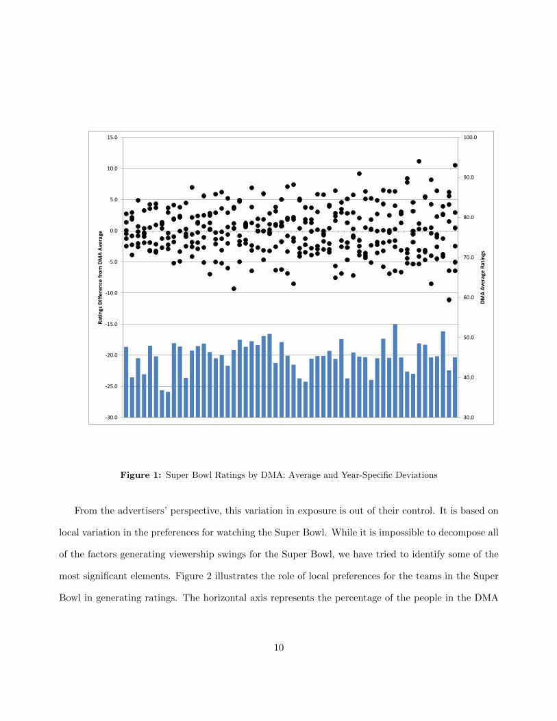
Figure 1 depicts substantial variation both across and within the top 56 DMAs in the exposures to the
Super Bowl ads.9 The bars at the bottom represent the average ratings for each DMA as measured
on the axis to the right. The average is 45.3 percent of a market viewing the Super Bowl, with cross-
market variation from 36.4 to 53.4 percent. The dots above represent the year by year deviations
from the DMA mean ratings as measured on the axis to the left. The DMAs are ordered left to right
with increasing variance in the ratings such that the DMA with the smallest variation across years
sees movement of roughly plus or minus 2.5 percent around its average ratings of 47.7 percent. Many
DMAs experience ratings dispersion of ten points or more, while the most variable DMAs experience
ratings dispersion of 17 points. Overall, this paints a picture of large swings in terms of how many
people are watching the Super Bowl and getting exposed to the ads.
8We’ve run our analysis also coding this up as an advertisement and while the coefficients change some, the substantiveconclusion remains the same.
9We focus our descriptives of the ratings data on the top 56 markets because the ratings data for smaller DMAsincludes a correctable measurement error described to us by the data provider. Specifically, reported ratings for smallermarkets represent an average across four weeks of viewership during the particular time slot. This lowers the reportedratings as all other airings during the time slot experience less viewership than the Super Bowl. Nevertheless, the SuperBowl’s size represents the majority of variation in this measure so enables us to capture the Super Bowl effect. We areable to correct for the measurement error because we know the true variance of the Super Bowl ratings from the largermarkets and therefore the error induced by this data collection aspect. These corrections are detailed in the code andwe also include a simple proof of concept program illustrating that our approach recovers the appropriate parameters.
9
30.0
40.0
50.0
60.0
70.0
80.0
90.0
100.0
-30.0
-25.0
-20.0
-15.0
-10.0
-5.0
0.0
5.0
10.0
15.0
DMA
Aver
age
Ratin
gs
Ratin
gs D
iffer
ence
from
DM
A Av
erag
e
Figure 1: Super Bowl Ratings by DMA: Average and Year-Specific Deviations
From the advertisers’ perspective, this variation in exposure is out of their control. It is based on
local variation in the preferences for watching the Super Bowl. While it is impossible to decompose all
of the factors generating viewership swings for the Super Bowl, we have tried to identify some of the
most significant elements. Figure 2 illustrates the role of local preferences for the teams in the Super
Bowl in generating ratings. The horizontal axis represents the percentage of the people in the DMA
10

who “liked” the two teams in the Super Bowl on Facebook as of April 2013.10 The vertical axis plots
the associated ratings for the Super Bowl. The relationship is clearly non-linear with more than 45
percent of the population watching whenever at least 5 percent of the market likes the teams. Among
those observations with less than 5 percent liking the team, there is still a correlation of 0.33 with the
observed ratings. This illustrates that preferences for the teams playing is still a significant driver of
viewership even outside the home cities.
This certainly does not explain all of the variation in ratings, as Facebook is not demographically
representative and we should ideally have these preference measures at the beginning of our data. To
quantify the explanatory power, we ran a simple regression of log ratings on the log of the percent
of the DMA liking the team. The R-squared is 0.24. Including both DMA and year fixed effects,
we find that the percent liking the team explains 12 percent of the within-DMA variation in ratings.
Year fixed effects alone explain about 42 percent of the within-market variation. The remainder of the
variation may arise from other unobserved components of the local preferences for the game. Some of
that variation occurs because we often measure likability of the teams well after the game was actually
played.
10While a better measure would include how many local people liked the teams before the respective Super Bowl, weare unaware of a historical source of such information that can date back to 2006.
11

30
35
40
45
50
55
60
0 5 10 15 20 25 30 35
Perc
ent o
f DM
A th
at W
atch
ed th
e Su
per
Bow
l
Percent of DMA that "Likes" Super Bowl teams on Facebook
Figure 2: Super Bowl Ratings by DMA: Average and Year-Specific Deviations
2.2 Retail Scanner Data
Nielsen’s retail scanner data provides unit sales, prices, display and feature information at the UPC
level for each store and week. While the UPCs can be aggregated at many levels (e.g. diet/light vs.
regular, sub-brand or pack size), we report our analysis aggregating sales to the brand level as we
expect that to internalize all of the effects of advertising.
We consider the top four brands (based on volume) in each category while aggregating the remain-
12
ing brands in a composite named “Other.”11 In beer, the focal brands are Budweiser, Miller, Coors
and Corona. These four brands also represent the top four purchasers of NFL impressions in weeks
prior to the Super Bowl. In soda, the focal brands are Coke, Pepsi, Dr. Pepper and Mountain Dew.
These brands also purchased the most NFL impressions prior to the Super Bowl.
We aggregate the store-level data to the geographic level at which we observe ratings, i.e. the
DMA. We consider up to twenty weeks after the Super Bowl, as well as the first five weeks of the year
leading up to the game on the first Sunday in February. The first week after the Super Bowl includes
Super Bowl Sunday. For each week in the data, we have included the DMA level gross rating points
(GRPs) for each brand’s advertising as reported by Nielsen’s AdViews. GRPs /100 are the number of
impressions per household. We also consider the cumulative GRPs during NFL games leading up to
the Super Bowl (Pre-SB NFL GRPs). This accounts for brand impressions that would be correlated
with Super Bowl ratings because the Super Bowl competitors also drew large audiences in previous
rounds of the playoffs. The outcome measures we focus on are volume and revenue. We similarly
analyze these on a per household basis where we calculate a constant number of households over the
six years in our data based on the GRPs and impressions reported in the advertising data.
Table 1 reports the outcomes and marketing decisions for the twenty weeks following the Super
Bowl. In the beer category, Budweiser clearly dominates their market with a revenue and volume
per household that is comparable to the combination of all brands outside of the top four.12 The
revenue and volume numbers represent only those households that might be covered by the Nielsen
sales data and thus translate into a number smaller than the actual revenue and volume per household.
The data is not necessarily representative as some stores, such as Walmart, are not included in the
Kilts data. Prices are comparable across the brands with the exception of Corona, an imported
11To avoid over-weighting large markets in selecting the top brands, we first ranked brands within market and weekand then selected those whose modal ranks were highest.
12The number of households is calculated and held fixed over time based on the median value reported by Nielsen forthe DMA across all six years.
13

beer priced nearly four cents per ounce more. The beers are featured roughly five percent of the time
(volume weighted), except for the Other category which includes smaller brands that may be unlikely to
promote themselves in stores circulars. Display rates are comparable to feature. Budweiser’s advertises
75% more than its closest competitor Miller with 0.007 impressions per capita. If no household saw
an ad more than once, this would translate to less than one percent of households seeing a Bud ad
in average week. This highlights the importance of the Super Bowl which reaches 45% of households.
Budweiser also purchased the most advertising impressions in NFL games leading up to the Super
Bowl. Coors comes in second at just over half of what Budweiser purchased.
In the soda category, Coke and Pepsi are the market leaders, but the Other category is substantially
larger than either of these brands in terms of both revenue and volume per household. Pricing in soda
is comparable across all brands. Major brands are featured 9 to 10 percent of the time, while the
Other brands are featured about 4 percent of the time. Displays occur 7 to 9 percent of the time for
major brands and just less than 5 percent of the time for Other brands. Pepsi is the leader in terms of
advertising purchased. Pepsi also purchased the most advertising during previous rounds of the NFL
playoffs, with Dr. Pepper following with nearly twice the NFL advertising as Coke.
3 Empirical Analysis
Our analysis is divided into three pieces. First, we analyze the brands consumers buy for consumption
while viewing the Super Bowl to test whether branded consumption is complementary with watching
the game or watching the brand’s ad during the game. Second, we estimate whether viewership of the
game (and hence the included ads) disproportionately increases post-Super Bowl sales for advertisers
relative to non-advertisers. These findings suggest Super Bowl ad effectiveness occurs in weeks when
consumers make purchases for consumption during subsequent sporting events. Finally, we collect
additional data on viewership of the NCAA basketball tournament to test whether viewership of
14

Table 1: Weekly Summary Statistics: 20 Post-Super Bowl Weeks
BeerVariable Budweiser Miller Coors Corona OtherRevenue per HH 0.322 0.114 0.091 0.057 0.332volume 6 pk 0.077 0.028 0.021 0.008 0.074price per oz 0.059 0.058 0.061 0.098 0.061feature 0.050 0.050 0.053 0.052 0.024display 0.054 0.047 0.049 0.053 0.024GRPs / 100 0.007 0.004 0.002 0.001 0.004Pre-SB NFL GRPs /100 0.164 0.058 0.095 0.009 0.026Observations across 173 DMAs and 20 weeks. Some DMA-years missing.DMAs with alcohold restrictions or negligible sales omitted.
SodaVariable Coke Pepsi Dr Pepper Mtn Dew OtherRevenue per HH 0.381 0.268 0.111 0.144 0.537volume 6 pk 0.209 0.158 0.060 0.077 0.288price per oz 0.026 0.025 0.027 0.028 0.027feature 0.093 0.105 0.021 0.041 0.036display 0.082 0.089 0.069 0.077 0.047GRPs / 100 0.007 0.007 0.003 0.002 0.004Pre-SB NFL GRPs / 100 0.006 0.020 0.012 0.001 0.001Observations across 191 DMAs and 20 weeks. Some DMA-years missing.
a Super Bowl ad increases the brand’s ability to capture more of the purchases that complement
viewership of the basketball games. The series of results identify advertising as a determinant of
brand-specific complementarities between beverage consumption and viewership of sports.
Each of these analyses considers how brand outcomes (volume or revenue per household) in a given
week and market relate to the market’s Super Bowl viewership. Market fixed effects crucially focus
inference on the year to year changes in Super Bowl viewership documented in the previous section
to arise from changes in preferences for watching the two teams who qualified for the championship.
We also include year fixed effects to avoid the possibility that aggregate viewership and brand sales
happened to be higher in one of the six years of our data. Finally, we include covariates describing
the brand’s local marketing activities in the focal week or prior to the Super Bowl.
We therefore estimate the following descriptive regression to analyze the relationship between the
volume or revenue per household13 (Y ), an indicator for whether brand j advertises in the Super Bowl
13We have also run the analyses below using volume per household and find the same substantive findings and signifi-cance patterns.
15

in year y (Ajy), and the fraction of the population that watched the Super Bowl in market m in year
y (Rmy).
Yjmyw = α1AjyRmy + δRmy +Xjmywβ + γFE + ξjmyw (1)
where j indexes the focal brand, m the market (DMA), y the year and w represents the week relative
to the Super Bowl, with w = 0 being the Sunday to Saturday week leading up to Super Bowl Sunday.
δ measures how variation in Super Bowl viewership affects the brand’s outcomes. α1 measures any
additional impact of viewership when brand j advertises in year y. We include weekly brand-market
specific covariates, Xjmyw to account for past and concurrent marketing efforts which after the game
could represent endogenous responses to the variation in ratings. Most of these are marketing variables
summarized in the previous section. γFE is the set of fixed effects discussed above. When we pool
multiple brands into the same analysis for comparison, we interact the above market and year fixed
effects with brand indicators.
We also estimate a pooled regression which recovers the average advertising effect, α1, across a
fixed number of weeks. The primary reason for this is to test for the significance of an average effect
when only some week specific effects are significant and to quantify an advertising elasticity that covers
a span of weeks after the game. In these cases, we introduce an additional fixed effect for the week
number relative to the Super Bowl.
3.1 Is Super Bowl Beverage Consumption Complementary to the Advertising orthe Game?
We test for complementarities between consumption of a brand and viewership of the Super Bowl.
In the absence of direct data on consumption during the game, we use observed purchases in the
week leading up to the game. The culture around Super Bowl parties and consumption of beer,
other beverages and snacks suggests complementarities exist. Our emphasis is to focus on differential
16

Super Bowl week purchases across brands of relatively homogenous goods (mass produced beers and
colas/carbonated beverages). Specifically, we consider why some brands might realize greater Super
Bowl week sales increases than others. Two differentiable theories can explain this. Yang, Allenby and
Fennel (2002) argue brands differ in their associations with certain consumption occasions. Presumably
branding activities such as advertising play a role in this development, but they do not explore that
in their analysis. We test this conjecture directly in section 3.3 below. On the other hand, Becker
and Murphy (1993) suggest a complementarity between brand consumption and viewership of the ad.
The testable implications of their theory are that brands advertising during the game should receive a
greater increase in consumption than non-advertisers. We illustrate below that i) brands which have
never advertised during the game also realize sales increases for consumption during the game, ii) Coca
Cola who advertised in the game for the last 5 years of our data never realizes Super Bowl sales for
consumption during the game, and iii) Pepsi’s and Coke’s Super Bowl sales are invariant to whether or
not they advertise in a given year. These results are inconsistent with the Becker and Murphy (1993)
theory, but supportive of Yang, Allenby and Fennel (2002)’s idea that some brands do, and other do
not, have associations with consumption occasions such as watching the Super Bowl.
To document the complementarities that exist, we apply Equation 1 to volume per household
outcomes in the beer and soda categories. The Ratings coefficient in columns (1) and (2) of Table 2
illustrate that Budweiser realizes substantial increases in volume per household in the Sunday through
Saturday leading up to Super Bowl Sunday, in those markets where realized Super Bowl ratings are
higher. Both coefficients being near to 0.1 indicates a 10 point increase in the ratings for the game
increases the amount of Budweiser consumed per household by one six-pack for every 100 households.
Note that this is likely an underestimate as we do not observe all sales because some large stores such
as Walmart are omitted from the data. Column (2) differs from (1) in that it controls for marketing
variables. We find price to be the only statistically significant factor. Columns (3) and (4) illustrate
17

that non-advertising brands also realize statistically significant increases in beer volume purchased in
anticipation of viewership, yet the effects are about a third the size. Finally, columns (5) and (6) pool
all brands together to illustrate that the incremental effect for Budweiser is about 0.07, or 7 extra six
packs per thousand households when ratings increase by ten points.14 The Ratings*Ad coefficients
in these specifications have p-values of 0.065 and 0.049 respectively. This leaves little doubt as to
Budweiser’s superior sales for consumption during the game.
Table 2: Volume of Beer Purchases in Anticipation of Super Bowl Viewership
Volume in Week Leading Up To Super Bowl(1) (2) (3) (4) (5) (6)
VARIABLES Bud Bud Non-Bud Non-Bud All All
Ratings 0.094* 0.103* 0.030* 0.032* 0.030* 0.032*(0.045) (0.041) (0.013) (0.013) (0.013) (0.012)
Ratings * Ad 0.064 0.071*(0.035) (0.036)
MarketingGRPs -0.006 -0.034 -0.058
(0.114) (0.158) (0.108)NFL GRPs -0.017 -0.019 -0.016
(0.027) (0.018) (0.024)Price -3.717** -0.680** -1.080**
(0.994) (0.125) (0.234)Price * Other -1.841** -1.446**
(0.500) (0.537)Feature -0.008 -0.001 -0.004
(0.034) (0.005) (0.008)Display -0.007 0.009 0.008
(0.033) (0.005) (0.007)Observations 888 888 3,552 3,552 4,440 4,440R-squared 0.101 0.280 0.102 0.287 0.102 0.233Number of branddma 173 173 692 692 865 865Fixed effects are included at the brand-market and brand-year.Standard errors are clustered at the market level.** p<0.01, * p<0.05
Becker and Murphy (1993) state that “the complementarity is obvious with beer advertising on
television during football games since many people drink beer as they watch a televised game.” We
argue that only the latter part of this statement is necessarily true. People drink many brands of beer,
14We allow the price coefficient to be different for the aggregation of all non-top 4 brands via the Price * Other Brandsinteractions because variation in this price also reflects variation in the relative volume of brands sold within the week.
18

whether advertised or not, when they watch the big game. These results provide stronger support
for the complementarity of beer brands generally with the consumption occasion. In fact, though not
reported here, the only one of the top four beer brands that does not exhibit a statistically significant
game-week volume increase with the Super Bowl ratings is Corona which has historically emphasized
beach settings as its associated consumption occasion.
The large incremental effects for the advertiser, Budweiser, may still however be consistent with
Becker and Murphy (1993) but we cannot specifically test this as we do not see Budweiser abstaining
from advertising during any given year. We therefore turn to the soda category where we document
both that one of the primary advertisers realizes no such game-week volume increases and the game-
week sales are invariant to whether or not the brands are advertising in the Super Bowl.
Columns (1) and (3) of Table 3 show that Coca-Cola realizes no statistically significant change
in soda volume in the week leading up to the Super Bowl. This holds whether or not Coca-Cola
advertised in the game and the direction of the coefficients suggests that tighter standard errors
would, if anything, imply a negative relationship. This is fully inconsistent with the Becker and
Murphy (1993) theory. Clearly from the beer analysis, and the results from Pepsi which we discuss
next, our data can identify consumption in anticipation of viewership. One might argue that because
Coca-Cola had not advertised prior to 2007, consumers were unaware Coca-Cola would be advertising.
But Coca-Cola’s entry was likely publicized and their many loyal customers would have been attune to
this by the second year, or at least by the end of the 5 consecutive years we observe them advertising
in our data. Yet, we have separately tested whether Coca-Cola might realize an increase over time in
game-week sales in the presence of higher ratings and found that their performance in game-week in
markets with higher ratings declines across years.
Pepsi on the other hand is seen to realize volume increases comparable to Budweiser’s. Columns
(2) and (4) test Pepsi’s game-week volume sales relationship with ratings both excluding and including
19

Table 3: Volume of Soda Purchases in Anticipation of Super Bowl Viewership
Volume in Week Leading Up To Super Bowl(1) (2) (3) (4) (5) (6) (7) (8)
VARIABLES Coke Pepsi Coke Pepsi Not CokePepsi Not CokePepsi All All
Ratings 0.034 0.037 0.036 0.039(0.032) (0.035) (0.032) (0.037)
Ratings * Ad 0.005 -0.002(0.009) (0.007)
Ratings * Coke -0.076 -0.072 -0.112 -0.116(0.077) (0.072) (0.072) (0.077)
Ratings * Ad * Coke -0.020 -0.030 -0.020 0.013(0.038) (0.033) (0.038) (0.032)
Ratings * Pepsi 0.166** 0.091 0.130** 0.084(0.064) (0.060) (0.047) (0.044)
Ratings * Ad * Pepsi -0.024 -0.025 -0.024 -0.009(0.030) (0.027) (0.030) (0.031)
MarketingGRPs -0.112 0.665 -1.161* 0.418
(0.253) (0.432) (0.470) (0.263)NFL GRPs -1.243** 0.613* -0.026 0.182
(0.362) (0.249) (0.074) (0.146)Price -21.211** -14.240** -4.916** -9.759**
(1.807) (1.947) (0.726) (0.969)Price * Other -1.516 3.408**
(1.114) (1.226)Feature 0.060 -0.053 0.017 0.070**
(0.037) (0.041) (0.019) (0.022)Display 0.012 0.077 0.008 -0.009
(0.046) (0.052) (0.022) (0.023)Observations 1,002 1,002 1,002 1,002 3,006 3,006 5,010 5,010R-squared 0.088 0.134 0.485 0.312 0.180 0.300 0.131 0.299Number of branddma 195 195 195 195 585 585 975 975Fixed effects are included at the brand-market and brand-year.Standard errors are clustered at the market level.** p<0.01, * p<0.05
20

marketing variables. The effects are large and statistically significant in (2) and marginally significant
in (4) with a p-value of 0.13. These results hold in (7) and (8) when we pool all soda brands together
and test for a difference between Pepsi and others. Pepsi is shown to have a statistically significant
greater game-week sales volume of roughly 0.13 without controlling for marketing activity. This
diminishes to 0.084 after controlling for marketing activity, yet still has a p-value of 0.059. The
marketing activity accounts for typical marketing mix variables as well as concurrent advertising
(GRPs) and advertising during prior NFL games in the playoff or regular season (NFL GRPs). An
effect of 0.1 would once again be an extra six pack per hundred households when the ratings increase
by ten points. Columns (5) and (6) and the top row of (7) and (8) document that no other brand
is observed to realize significant volume increases in the week before the game. Note that the Other
brands include non-Pepsi branded Pepsi-Cola company sodas that are typically jointly promoted in
store along with Pepsi.
The contrasting Super Bowl week performance of Coke and Pepsi supports our conjecture that
advertising is about building associations with consumption occasions and that Pepsi’s substantially
longer tenure advertising in the game has created that Super Bowl association while Coca-Cola has not.
This highlights a fundamental difference between a theory of advertising that itself is a complement
vs. our argument that the complementarity is with the occasion and firms advertise to “own” that.
Under complementarity with the ad, Coca-Cola’s loyal customers should have made purchases for
consumption during Coke Super Bowl ads, regardless of Pepsi’s history of advertising in the Super
Bowl. Yet, if brands seek to build complementarities with certain consumption occasions, Coke’s
Super Bowl advertising which ran side-by-side Pepsi in all but one year may have be unable to build
a long-run Coca-Cola association with the Super Bowl.
This section has documented complementarity of the brands with the consumption occasion follow-
ing Yang Allenby and Fennell (2002) and has cast considerable doubt on the advertising as complements
21

theory. Next, we turn to documenting the effects of the Super Bowl ads.
3.2 Super Bowl Advertising Effectiveness
In this sub-section, we evaluate whether the year-to-year variation in within market viewership of
the Super Bowl yields greater sales for advertisers than non-advertisers in post-Super Bowl weeks.
We begin by considering the path of advertising effectiveness across post-Super Bowl weeks. This
documents that the Super Bowl advertising effects are concentrated in weeks with subsequent sporting
events. To estimate elasticities that account for weeks with and without spikes in effectiveness, we
then estimate regressions that pool across multiple post-Super Bowl weeks.
3.2.1 Post-Super Bowl Weekly Advertising Effects
To avoid arbitrarily defining the window of Super Bowl advertising effectiveness, we estimate the
effect separately for each of the first 20 weeks following the Super Bowl. The weekly regression for
our analysis mirrors column (5) from Table 2, except that w > 0. Figure 3 plots the coefficient α1
(Ratings*Bud) from each week specific estimation of Equation 1 to show the differential effect of
Super Bowl viewership on advertisers’ vs. non-advertisers’ sales volume per household. The estimate
of α1 begins positive in week 1 and converges to zero by week 4. However, the effect increases to
be statistically significant in week 5. The coefficient remains positive, yet insignificant until week
10 after which it bumps up again. To reflect whether these volume increases also imply improved
returns, Figure 4 changes the dependent variable to revenue per household and we see significant
effects occurring in weeks 5, 8, 11, 14 and 16. These effects are quite large within the week they
occur in that the α1 coefficients for volume and revenue in week 5 of 0.03 and 0.15 indicate that a
ten point increase in ratings would increase volume and revenue by about 3.9 percent and 4.7 percent
respectively.
In seeking to understand why these advertising effects would show a resurgence in these particular
22

weeks, we found they coincide with subsequent sporting events. We discuss these events in more detail
after documenting similar patterns in the soda category.
We address the average effectiveness, elasticities and a full set of estimates and alternative speci-
fications in the next subsection.
-0.15
-0.10
-0.05
0.00
0.05
0.10
0.15
0.20
0.25
0.30
0.35
0.40
0.45
0.50
1 2 3 4 5 6 7 8 9 10 11 12 13 14 15 16 17 18 19 20 Reve
nue
per H
ouse
hold
Att
ribut
able
to S
uper
Bow
l Ad
View
ersh
ip
Week After the Super Bowl
Figure 3: Super Bowl Advertising Effect on Volume by Week After the Super Bowl: Budweiser
23

-0.15
-0.10
-0.05
0.00
0.05
0.10
0.15
0.20
0.25
0.30
0.35
0.40
0.45
0.50
1 2 3 4 5 6 7 8 9 10 11 12 13 14 15 16 17 18 19 20 Reve
nue
per H
ouse
hold
Att
ribut
able
to S
uper
Bow
l Ad
View
ersh
ip
Week After the Super Bowl
Figure 4: Super Bowl Advertising Effect on Revenue by Week After the Super Bowl: Budweiser
Next, we consider the weekly effectiveness of the Super Bowl ads for the soda category. In soda,
we restrict the analysis to Coke and Pepsi as they are most similar and are both observed in and out
of the Super Bowl. To allow the effects to vary by whether a competitor is also advertising during the
same game, we include an additional interaction we denote as α2 in the following expanded estimation
equation, and as Ratings * Ad * Ad in tables below. The estimating equation for advertising effects
in the soda category is therefore:
24

Yjmyw = α1AjyRmy + α2AjyAkyRmy + δRmy +Xjmywβ + γFE + ξjmy (2)
where Aky is an indicator for whether a competitor ran a Super Bowl ad that year. Aky does not
enter separately because there is no year in which no competitor offered an ad, so the effect of just
a competitor advertising is reflected in δ. Figure 5 plots α1 to document the pattern of Super Bowl
advertising effectiveness in the soda category over the post-Super Bowl weeks. The effect is significantly
positive in week 2, then declines until a resurgence in weeks 6, 8, 11, and 16 with 8 and 11 being
statistically significant. Rerunning the analysis with revenue as the dependent variable in Figure 6,
weeks 2, 6, 8, 11, 12 and 16 show statistically significant positive effects of Super Bowl ad viewership.
In soda there is clearly a large spike in effectiveness in week 8 which corresponds with both the
NCAA Final Four and the opening week of Major League Baseball. The confidence intervals indicate
that this is significantly greater than the advertising effect in the preceding weeks. Other spikes in
weeks 6, 11 and 16 correspond with the beginning of the NCAA basketball tournament, the NBA
Playoffs and the NBA Finals.
We note that we did not hypothesize this timing and resurgence of effects, but we do use these
suggestive patterns to formally test the relevance of Super Bowl ads for consumption during sports in
section 3.3.
25

-0.15
-0.10
-0.05
0.00
0.05
0.10
0.15
0.20
0.25
0.30
0.35
0.40
0.45
0.50
1 2 3 4 5 6 7 8 9 10 11 12 13 14 15 16 17 18 19 20
Volu
me
per H
ouse
hold
Att
ribut
able
to a
Per
cent
age
Poin
t Inc
reas
e in
Exp
osed
Hou
seho
ld
Week After the Super Bowl
Figure 5: Super Bowl Advertising Effect on Volume by Week After the Super Bowl: Coke & Pepsi AdvertisingAlone
26

-0.15
-0.10
-0.05
0.00
0.05
0.10
0.15
0.20
0.25
0.30
0.35
0.40
0.45
0.50
1 2 3 4 5 6 7 8 9 10 11 12 13 14 15 16 17 18 19 20
Reve
nue
per H
ouse
hold
Att
ribut
able
to a
Per
cent
age
Poin
t Inc
reas
e in
Exp
osed
Hou
seho
ld
Week After the Super Bowl
Figure 6: Super Bowl Advertising Effect on Revenue by Week After the Super Bowl: Coke & Pepsi AdvertisingAlone
3.2.2 Average Effect of Super Bowl Ads
Before moving on to explicit tests of the effectiveness arising from the Super Bowl building an associa-
tion with sports viewership more broadly, we pool these weekly observations into regressions that allow
us to test for average effectiveness, estimate proper elasticities and show the full set of estimates from
a variety of specifications. We focus on a two month (eight-week) window because this time frame
27

provides robustness across nearly all specifications we have tried15 and this summarizes the average
effects up to the highest peak of advertising effectiveness in each category.
In this analysis, each week separately enters the regressions, rather than aggregating the weekly
data. This allows the effects of weekly marketing variables to exhibit their contemporaneous rela-
tionships with outcomes. We begin by separately considering advertising and non-advertising brands.
Then, we combine them in a regression to establish statistical significance of the differential perfor-
mance of the advertising brands relative to non-advertisers. These latter regressions represent the
average effect of the weekly regressions plotted in the figures above.
The first specification in Table 4 considers only Budweiser observations and evaluates how their
weekly volume per household varies with ratings for the Super Bowl. The 0.018 Ratings * Ad coefficient
indicates that Budweiser receives a volume increase of nearly 2 six-packs per thousand households
for every 10 point increase in Super Bowl ratings (i.e. ratings are measured as the fraction of the
population who watched the game). In column (2) we add covariates and find this effect to increase
to 0.026 with a p-value of 0.05. The fit of the regression increases with the inclusion of significant
predictors such as price and feature. Note that we cannot interpret the coefficients on the marketing
variables causally because we do not have exogenous variation in these. Nevertheless, they make
clear that the primary marketing variables of the firm are not exhibiting an endogenous response to
the Super Bowl ad viewership that is driving the estimates. Specifications (3) and (4) replicate the
preceding regressions for all non-Budweiser brands. There is no evidence of a significant increase or
decrease in these brands’ performance that can be attributed to Super Bowl viewership. Specifications
(5) and (6) pool all brands together to illustrate this significant difference for the advertising brand,
Budweiser, relative to competitors. Specification (5) is roughly the average effect over the first 8 weeks
plotted in Figure 3. These effects in columns (5) and (6) imply an advertising elasticity of about 0.1.
28

Table 4: Effects of Super Bowl Viewership and Advertising on Beer Volume
8 Weeks Post-Super Bowl Included(1) (2) (3) (4) (5) (6)
VARIABLES Bud Only Bud Only Non-Bud Non-Bud All Brands All Brands
Ratings -0.000 0.001 -0.000 0.001(0.006) (0.006) (0.006) (0.006)
Ratings * Ad 0.018 0.026 0.019* 0.019*(0.012) (0.013) (0.009) (0.009)
MarketingGRPs 0.030 -0.008 -0.009
(0.020) (0.010) (0.011)NFL GRPs 0.001 -0.004 0.000
(0.005) (0.004) (0.004)Price -2.927** -0.353** -0.627**
(0.501) (0.043) (0.087)Price * Other -0.849** -0.624**
(0.221) (0.215)Feature 0.040** 0.002 0.005*
(0.012) (0.001) (0.002)Display -0.015 0.007 0.005
(0.015) (0.004) (0.005)Observations 7,104 7,104 28,411 28,411 35,515 35,515R-squared 0.222 0.361 0.155 0.225 0.164 0.219Number of branddma 173 173 692 692 865 865Fixed effects are included at the brand-market, brand-year and week relative to the Super Bowl.Standard errors are clustered at the market level.** p<0.01, * p<0.05
29
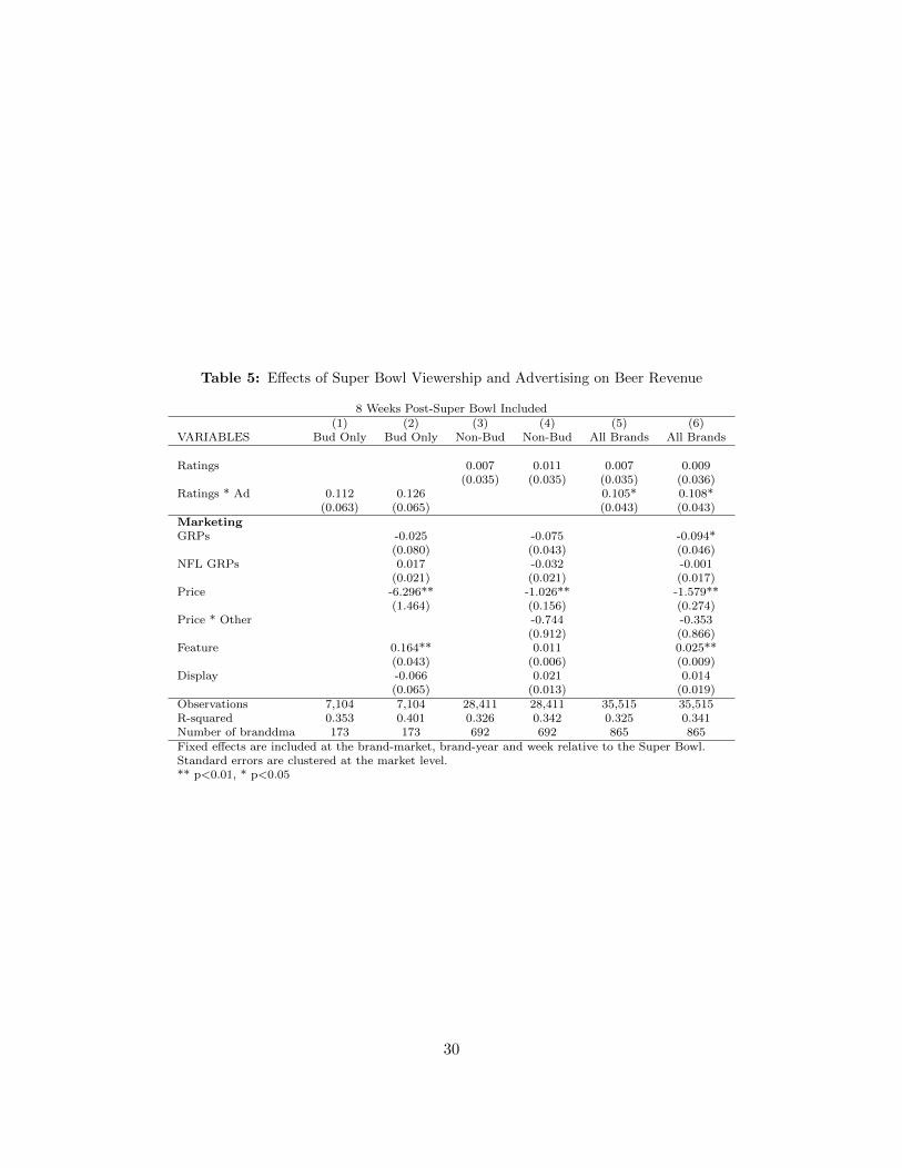
Table 5: Effects of Super Bowl Viewership and Advertising on Beer Revenue
8 Weeks Post-Super Bowl Included(1) (2) (3) (4) (5) (6)
VARIABLES Bud Only Bud Only Non-Bud Non-Bud All Brands All Brands
Ratings 0.007 0.011 0.007 0.009(0.035) (0.035) (0.035) (0.036)
Ratings * Ad 0.112 0.126 0.105* 0.108*(0.063) (0.065) (0.043) (0.043)
MarketingGRPs -0.025 -0.075 -0.094*
(0.080) (0.043) (0.046)NFL GRPs 0.017 -0.032 -0.001
(0.021) (0.021) (0.017)Price -6.296** -1.026** -1.579**
(1.464) (0.156) (0.274)Price * Other -0.744 -0.353
(0.912) (0.866)Feature 0.164** 0.011 0.025**
(0.043) (0.006) (0.009)Display -0.066 0.021 0.014
(0.065) (0.013) (0.019)Observations 7,104 7,104 28,411 28,411 35,515 35,515R-squared 0.353 0.401 0.326 0.342 0.325 0.341Number of branddma 173 173 692 692 865 865Fixed effects are included at the brand-market, brand-year and week relative to the Super Bowl.Standard errors are clustered at the market level.** p<0.01, * p<0.05
30
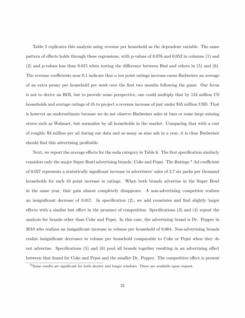
Table 5 replicates this analysis using revenue per household as the dependent variable. The same
pattern of effects holds through these regressions, with p-values of 0.076 and 0.052 in columns (1) and
(2) and p-values less than 0.015 when testing the difference between Bud and others in (5) and (6).
The revenue coefficients near 0.1 indicate that a ten point ratings increase earns Budweiser an average
of an extra penny per household per week over the first two months following the game. Our focus
is not to derive an ROI, but to provide some perspective, one could multiply that by 124 million US
households and average ratings of 45 to project a revenue increase of just under $45 million USD. That
is however an underestimate because we do not observe Budweiser sales at bars or some large missing
stores such as Walmart, but normalize by all households in the market. Comparing that with a cost
of roughly $3 million per ad during our data and as many as nine ads in a year, it is clear Budweiser
should find this advertising profitable.
Next, we report the average effects for the soda category in Table 6. The first specification similarly
considers only the major Super Bowl advertising brands: Coke and Pepsi. The Ratings * Ad coefficient
of 0.027 represents a statistically significant increase in advertisers’ sales of 2.7 six packs per thousand
households for each 10 point increase in ratings. When both brands advertise in the Super Bowl
in the same year, that gain almost completely disappears. A non-advertising competitor realizes
an insignificant decrease of 0.017. In specification (2), we add covariates and find slightly larger
effects with a similar lost effect in the presence of competition. Specifications (3) and (4) repeat the
analysis for brands other than Coke and Pepsi. In this case, the advertising brand is Dr. Pepper in
2010 who realizes an insignificant increase in volume per household of 0.004. Non-advertising brands
realize insignificant decreases in volume per household comparable to Coke or Pepsi when they do
not advertise. Specifications (5) and (6) pool all brands together resulting in an advertising effect
between that found for Coke and Pepsi and the smaller Dr. Pepper. The competitive effect is present
15Some results are significant for both shorter and longer windows. These are available upon request.
31

in these specifications as well. The advertising elasticity implied by Coke or Pepsi advertising alone
in the Super Bowl is between 0.03 and 0.08 depending on whether the effect in specification (6) or (2)
is used.
Table 6: Effects of Super Bowl Viewership and Advertising on Soda Volume
8 Weeks Post-Super Bowl Included(1) (2) (3) (4) (5) (6)
VARIABLES Coke-Pepsi Coke-Pepsi Not Coke-Pepsi Not Coke-Pepsi All Brands All Brands
Ratings -0.017 -0.023 -0.012 -0.001 -0.014 -0.005(0.024) (0.023) (0.016) (0.016) (0.018) (0.017)
Ratings * Ad 0.027** 0.037** 0.004 -0.002 0.016** 0.014**(0.010) (0.008) (0.003) (0.003) (0.005) (0.004)
Ratings * Ad*Ad -0.023* -0.035** -0.017* -0.019**(0.009) (0.008) (0.008) (0.007)
MarketingGRPs -0.101* -0.045 -0.155**
(0.047) (0.062) (0.044)NFL GRPs -0.170 0.052 -0.050
(0.135) (0.035) (0.074)Price -14.109** -4.430** -8.426**
(0.854) (0.350) (0.551)Price * Other -1.823 2.252*
(1.114) (1.069)Feature 0.082** 0.077** 0.123**
(0.025) (0.015) (0.021)Display -0.030 0.012 -0.027
(0.026) (0.012) (0.018)Observations 16,032 16,032 24,048 24,048 40,080 40,080R-squared 0.076 0.379 0.082 0.230 0.071 0.281Number of branddma 390 390 585 585 975 975Fixed effects are included at the brand-market, brand-year and week relative to the Super Bowl.Standard errors are clustered at the market level.** p<0.01, * p<0.05
Table 7 replicates this analysis using revenue per household as the dependent variable. The same
pattern of effectiveness holds with advertising GRPs, price and feature being the marketing variables
showing a statistically significant relationship. The relationship for GRPs is negative, but since we do
not have causal variation in the GRPs this may reflect that ads were more likely to be broadcast or
viewed where soda brands had trouble generating sales. This highlights the importance of exogenous
variation for measuring advertising effects, such as our focus for the Super Bowl advertising. The
32

Table 7: Effects of Super Bowl Viewership and Advertising on Soda Revenue
8 Weeks Post-Super Bowl Included(1) (2) (3) (4) (5) (6)
VARIABLES Coke-Pepsi Coke-Pepsi Not Coke-Pepsi Not Coke-Pepsi All Brands All Brands
Ratings -0.059 -0.064 -0.051 -0.044 -0.054 -0.046(0.037) (0.038) (0.038) (0.039) (0.036) (0.036)
Ratings * Ad 0.077** 0.087** 0.012* 0.007 0.047** 0.044**(0.013) (0.014) (0.006) (0.006) (0.008) (0.007)
Ratings * Ad*Ad -0.036* -0.053** -0.020 -0.025*(0.015) (0.012) (0.013) (0.011)
MarketingGRPs 0.034 -0.493** -0.177**
(0.068) (0.119) (0.060)NFL GRPs -0.368 0.077 -0.125
(0.214) (0.068) (0.114)Price -14.505** -4.310** -8.523**
(0.925) (0.374) (0.577)Price * Other 0.423 4.711**
(1.501) (1.502)Feature 0.140** 0.099** 0.170**
(0.033) (0.020) (0.028)Display -0.041 0.021 -0.027
(0.035) (0.015) (0.022)Observations 16,032 16,032 24,048 24,048 40,080 40,080R-squared 0.093 0.315 0.390 0.437 0.215 0.335Number of branddma 390 390 585 585 975 975Fixed effects are included at the brand-market, brand-year and week relative to the Super Bowl.Standard errors are clustered at the market level.** p<0.01, * p<0.05
33

primary difference in the revenue analyses relative to volume is that only about half the gain from
advertising during a Super Bowl is lost when both Coke and Pepsi advertise in the same game.
Both the volume and revenue regressions show that advertising in the Super Bowl can be profitable,
but that there are substantial competitive effects. These highly competitive advertising effects are
consistent with our suggestion that brands use advertising to compete for associations with particular
consumption occasions. If both brands advertise head to head, it would seem challenging for either
brand to make progress in “owning” the relevant associations.
3.3 Advertising and the Complementarity Between Brands and Sports
Section 3.1 rejects the Becker and Murphy (1993) theory that advertising itself is a complement in
the case of Super Bowl advertising, but here we ask whether advertising builds complementarity
between the brand and sports viewership more broadly. We developed this hypotheses based on the
the temporal patterns observed in section 3.2 and test it by collecting subsequent sports viewership
data.
Specifically, we collected data on viewership of the NCAA basketball tournament, which can span
across weeks 4 through 10, depending on the year. We chose to focus on the NCAA tournament for
two reasons. First, it occurs the soonest after the game, such that the effects have the potential to
be the greatest. Second, NCAA broadcasts are aired across many network television channels (e.g.
ABC, CBS, NBC and Fox) such that the viewership is measurable in Nielsen ratings data. Major
League Baseball, for example, would have been difficult to analyze because the teams primarily air
their games on local cable networks where ratings data are unavailable to us.
To include the effects of NCAA viewership in our model, we run regressions that pool weekly
observations as in the last section, but use the entire time span of our data. The empirical specification
is extended to include the NCAA viewership variable by itself, then interacted with the major brands
in the category, and finally interacted with all of the Super Bowl ratings related coefficients from above.
34

To be clear, the hypothesis is that if Super Bowl advertising builds a complementarity between the
brand and sports viewership more broadly, the interaction NCAA * Ratings * Ad should be positive.
Our estimates are reported in Table 8. We begin in specification (1) with the beer category
and a replication of the analysis from the last section with the entire 20 week time span of our
data. Specification (2) adds covariates and we find the Ratings * Ad coefficient to still be significant.
Specification (3) introduces the NCAA viewership data, with the interaction of Ratings * Ad with
NCAA viewership in the fifth row. It is positive and statistically significant indicating support for
the viewership of Super Bowl advertising building a complementarity between the brand and sports
viewership. (4) adds covariates in and the results are unchanged. Columns (5) to (7) repeat this
analysis for Coke and Pepsi observations. Similarly wee see that NCAA * Ratings * Ad coefficient is
significantly positive. In line with the competitive effects documented above, the NCAA * Ratings *
Ad * Ad coefficient shows this relationship disappears when both competitors advertise in the Super
Bowl.
To summarize these findings, Super Bowl advertising increases a brand’s ability to capture sales
when consumer’s make purchases for consumption during subsequent sporting events.
3.4 Discussion and Caveats
There are some selection possibilities that deserve discussion. We conduct our analysis using variation
in ratings alone, conditional on a Super Bowl ad being aired. The two deviations in each soda brand’s
typical advertising decision are not likely candidates for a selection bias. Coca-Cola did not advertise
in the first year in our data (2006), but advertised in all subsequent years. As they had not advertised
since 1998, it does not appear they cherry-picked the year in our data in which they did not advertise.
Furthermore, the brand-year fixed effect would pick up any common demand shock to Coca-Cola in
2006 that might have led them to not advertise. The fixed effects therefore force selection concerns to
35

Table 8: Testing Super Bowl Ad Viewership Interaction with NCAA Viewership on Volume
20 Weeks Post-Super Bowl Included(1) (2) (3) (4) (5) (6) (7) (8)
VARIABLES Beer Beer Beer Beer Coke-Pepsi Coke-Pepsi Coke-Pepsi Coke-Pepsi
Ratings -0.001 -0.001 -0.000 0.001 -0.031 -0.029 -0.026 -0.031(0.006) (0.007) (0.006) (0.007) (0.026) (0.029) (0.027) (0.030)
Ratings * Ad 0.016 0.017 0.015 0.016 0.011 0.016* -0.004 0.008(0.009) (0.009) (0.009) (0.009) (0.007) (0.007) (0.008) (0.008)
Ratings * Ad*Ad -0.004 -0.006 0.007 -0.000(0.009) (0.000) (0.000) (0.000)
NCAA * Ratings -0.086** -0.088** -0.252** -0.013(0.022) (0.022) (0.109) (0.069)
NCAA * Ratings * Ad 0.121** 0.118** 0.579** 0.309**(0.022) (0.022) (0.109) (0.080)
NCAA * Ratings * Ad*Ad -0.406** -0.257**(0.076) (0.057)
NCAA 0.041** 0.044** 0.220** 0.110**(0.008) (0.008) (0.027) (0.026)
NCAA * Bud -0.077** -0.076**(0.009) (0.009)
NCAA * Pepsi -0.171** -0.078**(0.024) (0.020)
MarketingGRPs -0.102** -0.088** 0.113* 0.034
(0.028) (0.028) (0.053) (0.055)NFL GRPs 0.003 0.002 -0.104 -0.100
(0.004) (0.004) (0.137) (0.137)Price -0.710** -0.715** -14.710** -14.670**
(0.091) (0.091) (0.915) (0.914)Price * Other -0.382* -0.372*
(0.182) (0.183)Feature 0.008** 0.008** 0.095** 0.095**
(0.003) (0.003) (0.025) (0.025)Display 0.004 0.004 0.001 0.001
(0.005) (0.005) (0.033) (0.033)Observations 88,795 88,795 88,795 88,795 40,080 40,080 40,080 40,080R-squared 0.251 0.285 0.255 0.288 0.107 0.398 0.111 0.399Number of branddma 865 865 865 865 390 390 390 390Fixed effects are included at the brand-market, brand-year and week relative to the Super Bowl.Standard errors are clustered at the market level.** p<0.01, * p<0.05.
36

Table 9: Testing Super Bowl Ad Viewership Interaction with NCAA Viewership on Revenue
20 Weeks Post-Super Bowl Included(1) (2) (3) (4) (5) (6) (7) (8)
VARIABLES Beer Beer Beer Beer Coke-Pepsi Coke-Pepsi Coke-Pepsi Coke-Pepsi
Ratings 0.003 0.003 0.008 0.008 -0.071 -0.070 -0.071 -0.075(0.038) (0.038) (0.038) (0.038) (0.038) (0.041) (0.039) (0.042)
Ratings * Ad 0.103* 0.109* 0.099* 0.104* 0.052** 0.059** 0.034** 0.049**(0.044) (0.045) (0.044) (0.045) (0.009) (0.011) (0.009) (0.011)
Ratings * Ad*Ad -0.005 -0.015 0.012 -0.003(0.014) (0.010) (0.014) (0.010)
NCAA * Ratings -0.393** -0.400** -0.167 0.091(0.085) (0.085) (0.102) (0.086)
NCAA * Ratings * Ad 0.438** 0.431** 0.712** 0.420**(0.086) (0.086) (0.135) (0.110)
NCAA * Ratings * Ad*Ad -0.662** -0.499**(0.106) (0.091)
NCAA 0.184** 0.193** 0.295** 0.171**(0.036) (0.036) (0.036) (0.037)
NCAA * Bud -0.282** -0.277**(0.036) (0.035)
NCAA * Pepsi -0.214** -0.108**(0.032) (0.027)
MarketingGRPs -0.363** -0.318** 0.196** 0.086
(0.120) (0.117) (0.069) (0.072)NFL GRPs 0.006 0.005 -0.328 -0.321
(0.018) (0.018) (0.210) (0.210)Price -1.855** -1.873** -15.739** -15.682**
(0.314) (0.313) (0.974) (0.972)Price * Other 0.701 0.738
(0.827) (0.829)Feature 0.035** 0.035** 0.140** 0.141**
(0.010) (0.010) (0.032) (0.032)Display 0.011 0.011 0.005 0.005
(0.018) (0.018) (0.041) (0.041)Observations 88,795 88,795 88,795 88,795 40,080 40,080 40,080 40,080R-squared 0.352 0.364 0.355 0.367 0.095 0.318 0.100 0.320Number of branddma 865 865 865 865 390 390 390 390Fixed effects are included at the brand-market, brand-year and week relative to the Super Bowl.Standard errors are clustered at the market level.** p<0.01, * p<0.05.
37

imply that a brand chose to advertise or not based on its expectations of the cross-market distribution
of Super Bowl viewership relative to that occurring in other years. Suppose the brand has little
potential to convert customers in politically left-leaning “blue” states, then it might withdraw from
the Super Bowl in a year when the competing teams will be from San Francisco and New York. This
clearly cannot describe Coca-Cola’s extended absence pre-2007 and persistence in the game ever since.
Pepsi on the other hand has only been absent in one year, 2010. There is however a lot of information
about this exit. Pepsi decided to shift both its Super Bowl budget, and a significant portion of the
rest of its marketing budget, to fund a social media campaign (the Pepsi Refresh campaign) that gave
grants to proposals to help local communities, the environment etc.. A Harvard Business School case
and the news articles it cites nicely describe this decision as about shifting emphasis to social causes
and not about a poor Super Bowl opportunity. In fact they announced the decision before the end
of the NFL’s regular season.16 It is therefore highly unlikely that this was driven by an accurate
expectation of which of the NFL teams would eventually make it to the Super Bowl. Pepsi did return
the following year when the Pepsi Refresh campaign failed to live up to Pepsi’s expectations.
It is possible that advertisers could alter other factors about their advertising in response to the
anticipated distribution of Super Bowl viewership. They could change the creative execution of the
ad, but the expense of developing creative for Super Bowls suggests this is unlikely in the weeks just
before the game. They could also alter the number of spots aired during the game. We can observe
this and have run specifications with this included, but prefer to focus our analysis around the ratings
data whose variation is exogenous. The brands could also alter the particular products they choose
to advertise in the game. Pepsi occasionally advertises Diet Pepsi or Pepsi Max, and Anheuser-Busch
has used some of its many spots in a year to include other brands such as Michelob or Stella. These
could have also been chosen strategically based on the anticipated distribution of viewership. While
16A Wall Street Journal article titled “Pepsi Benches its Drinks” detailed the move on December 17, 2009, which isthree weeks before the end of the regular season.
38

we cannot rule out these selection decisions, we are skeptical they exist. They may bias upward the
estimates of the Super Bowl ad effect in beer, but its unlikely they account for a majority of it. In
soda, it is hard to imagine that such selection decisions would be driving the link between Super Bowl
viewership and sales in the particular weeks exhibiting spikes in Figure 6; and that these timed spikes
would only occur in years the soda brand is advertising.
It may also be argued that the post-Super Bowl performance of advertisers in high viewership
markets reflects a lasting effect from their greater consumption during the game. Such an effect could
be rationalized by habit persistence or switching costs, but i) such behavior is known to be difficult to
identify in aggregate data, ii) the above effects are much greater than others have found for packaged
goods (see Dube, Hitsch and Rossi, 2010), and iii) it is also inconsistent with some of the greatest effects
occurring 5 or 8 weeks later. Furthermore, we observe non-advertising beer brands realizing Super
Bowl consumption during the game, but not post-Super Bowl sales effects of Super Bowl viewership.
Finally, there might be some concern about measurement error in the market-level ratings data.
This does not however seem to be a problem as we are finding large effects. We could have used the
Facebook likings of the competing teams as an instrument to remove such errors, but the first-stage
incremental fit is too small and greatly increases standard errors (see Rossi, 2014 for a discussion of
the problems with using weak instruments when there is little endogeneity concern). We have also
tested for measurement error by allowing coefficients to be interacted with number of households in
the market. Smaller markets in the data should exhibit more measurement error as there are fewer
local Nielsen panelists to form the share of household viewership numbers. We did not however find
this to affect the results.
39

4 Conclusion
Advertising is one of the most important instruments a brand can use to market its products, yet
advertising’s efficacy and the mechanisms behind it are highly disputed. The benefits for a new product
are clear as consumers might otherwise be unaware of its existence and features. For established
brands, the incentive to spend on uninformative advertising such as that observed in the Super Bowl
has been questioned. Using exogenous variation in the viewership of the Super Bowl, we document
that established brands can realize substantial advertising effects with elasticities on the order of 0.03
to 0.1.
The pattern of Super Bowl advertising effectiveness over time also uncovers the source of effec-
tiveness and competitive implications. Advertising can build or reinforce a complementarity between
a brand and potential consumption occasions. Consumption of beer, snacks and other items while
watching sports is easily observed in society. Previous work suggests this arises from the desire to con-
sume a brand while watching its ad. We document that both advertising and non-advertising brands
realize this complementarity and that some advertising brands never do. Rather, our results provide
what we believe is the first evidence illustrating that advertising plays a role in the complementarity
between sports viewership and consumption and that it can link the complementarity to a particular
brand. Competition for such a strong branding association in the soda category is however shown to
be dissipative which can rationalize Budweiser’s procurement of exclusivity in Super Bowl advertising.
Finally, we uncovered the above advertising effects and patterns by exploiting data variation in
the Super Bowl context that may have parallels more broadly. The key to our identification is that
within market variation in exposures to a national broadcast represents valuable exogenous variation.
The national broadcast prevents market specific targeting of the advertising and thereby eliminates a
primary source of endogeneity. One might imagine applying our strategy to a cross-section, but the
distribution of viewership could be cross-sectionally associated with the distribution of consumption
40

(e.g. markets that watch a lot of football also consume a lot of beer). By analyzing within market,
cross-time variation, such correlations are removed. Interestingly, such a correlation can safely be the
source of the advertising decision as long as the advertising decision covers multiple time periods or
is invariant across time as we see for Budweiser and most years of Coke and Pepsi’s strategies. This
logic suggests other applications such as the common purchase of national advertising in “upfronts”
months before an event or TV program’s “season” begins. Week to week variation in viewership of
Monday Night Football or even dramas could be reasonably exogenous as long as there is not spurious
correlation between the weekly viewership and consumption or purchase on subsequent days. The
challenge in these settings is to address the reach and frequency dynamics that likely persist across
weeks, yet which we could safely ignore across the twelve months between which a Super Bowl occurs.
This, and the challenges of integrating other advertising, therefore represents some of the work still
needed to fully incorporate these insights into the marketing mix models measurement firms estimate.
41
References
[1] Aaker, J. (1997), “Dimensions of Brand Personality,” Journal of Marketing Research, XXXIV, 347-356.
[2] Ackerberg, D. (2001), “Empirically Distinguishing Informative and Prestige Effects of Advertising,” RANDJournal of Economics, 32(2), 316-333.
[3] Bagwell, K. (2007), “The Economic Analysis of Advertising,” Handbook of Industrial Organization, vol. 3,1701-1844.
[4] Becker, G. and K. Murphy (1993), “A Simple Theory of Advertising,” Quarterly Journal of Economics,108(4), 941-964.
[5] Bertrand, M., et.al. (2010), “What’s Advertising Content Worth? Evidence from a Consumer CreditMarketing Field Experiment,” The Quarterly Journal of Economics, 125(1), 263-306.
[6] Bronnenberg, B., M. Kruger and C. Mela (2008), “The IRI Marketing Data Set,” Marketing Science, 27(4),745-748.
[7] Bronnenberg, B., S. Dhar and J.P. Dube, (2009), “Brand History, Geography, and the Persistence of BrandShares,” Journal of Political Economy, 117(1), 87-115.
[8] Crupi, A. (2012), “CBS Halfway to a Super Bowl Sellout,” AdWeek.
[9] Doganoglu, T. and D. Klapper (2006), “Goodwill and Dynamic Advertising Strategies,” Quantitative Mar-keting and Economics, 4(1), 5-29.
[10] Doraszelski, U. and S. Markovich (2007), “Advertising Dynamics and Competitive Advantage,” RandJournal of Economics, 38(3), 557-592.
[11] Dube, J. P., G. Hitsch and P. Manchanda (2005), “An Empirical Model of Advertising Dynamics,” Quan-titative Marketing and Economics, 3(2), 107-144.
[12] Dube, J. P., G. Hitsch and P. Rossi (2010), “State Dependence and Alternative Explanations for ConsumerInertia,” RAND Journal of Economics, 41(3), 417-445.
[13] Fennell (1997), “Value and values: Relevance to advertising,” L. Kahle, L. Chiagouris, eds. Values,Lifestyles, and Psychographics, Erlbaum, Hillsdale, NJ.
[14] Hendel, I. and A. Nevo (2003), “The Post-Promotion Dip Puzzle: What do the Data Have to Say?”Quantitative Marketing and Economics, 1(4), 409-424.
[15] Lewis, R. and J. Rao (2014), “The Unfavorable Economics of Measuring the Returns to Advertising,”working paper.
[16] Lewis, R. and D. Reiley (2013), “Down to the Minute Effect of Super Bowl Advertising on Online SearchBehavior,” 14th ACM Conference on Electronic Commerce 9(4) Article 61.
[17] Lodish, L., M. Abraham, S. Kalmenson, J. Livelsberger, B. Lubetkin, B. Richardson, and M. E. Stevens(1995), “How T.V. Advertising Works: A Meta-Analysis of 389 Real World Split Cable T.V. AdvertisingExperiments,” Journal of Marketing Research, 32(2), 125-139.
[18] Nerlove, M. and K.J. Arrow (1962), “Optimal Advertising Policy Under Dynamic Conditions,” Economica,29(114), 129-142.
[19] Rossi, P.E. (2014), “Even the Rich Can Make Themselves Poor: a critical examination of the use of IVmethods in marketing,” Marketing Science, 33(5), 655-672.
[20] Sahni, N. (2013), “Effect of Temporal Spacing Between Advertising Exposures: Evidence from an OnlineField Experiment,” working paper.
42


![FRW holography from uplifted AdS/CFT - · PDF fileFRW holography from uplifted AdS/CFT Gonzalo Torroba SLAC, Stanford University Based on arXiv: 1108.5732 [DHMST], 1005.5403 [DHST]](https://static.fdocuments.us/doc/165x107/5a822f967f8b9ada388dae1c/frw-holography-from-uplifted-adscft-holography-from-uplifted-adscft-gonzalo.jpg)