Summary of the Environmental Impact Statement for the New Nuclear
50
Price Discrimination 2.0: Opaque Bookings in the Hotel Industry * Ricardo Cossa Mariano Tappata This draft: November 27, 2013 Abstract The emergence of opaque selling (i.e., when a product characteristic is only revealed to the customer after payment) has motivated a growing theoretical literature but little progress on the empirical front. This paper tries to fill this gap. We document the main features of opaque selling using a unique dataset from the lodging industry that includes bookings made in opaque platforms— Priceline and Hotwire—matched to their equivalent booking in the transparent market. We argue that opaque platforms allow hotels to achieve demand seg- mentation across-channels instead of using within-channel intertemporal price discrimination strategies. Opaque discounts relative to a transparent booking vary across selling channels and hotel quality segments. Consistent with con- sumer self-selection based on transaction costs and dispersion of preferences over transparent products, the average opaque discounts 40% in the posted- price platform and 49% in the auction-based platform. We find weak evidence of price-skimming strategies traditionally associated to revenue management practices in the travel industry. Moreover, we reject the hypothesis that hotels use opaque selling as a last-minute resource to dispose unsold inventory. JEL Codes: D43, D47, L11, M31. Keywords: Two-sided markets, Opaque platforms, Price discrimination, Lodg- ing Industry, Hotwire, Priceline. * Correspondence to Mariano Tappata: Strategy and Business Economics Division, Sauder School of Business, University of British Columbia. 2053 Main Mall, Vancouver, BC; Canada, V6T–1Z2. E-mail: [email protected]. Ricardo Cossa: Charles Rivers Associates, E-mail: [email protected]. We thank Mariana Marchionni for insightful discussions. Thanks also to Pascal Courty, Vera Brenˇ ciˇ c, Marco Celentani, Nathan Schiff and seminar participants at various institu- tions for helpful comments. Mariano Tappata is grateful for financial support from SSHRC. Please go to https://sites.google.com/site/marianotappata/research for the latest draft of this paper. 1
Transcript of Summary of the Environmental Impact Statement for the New Nuclear

Price Discrimination 2.0: Opaque Bookings in the
Hotel Industry∗
Ricardo Cossa Mariano Tappata
This draft: November 27, 2013
Abstract
The emergence of opaque selling (i.e., when a product characteristic is only
revealed to the customer after payment) has motivated a growing theoretical
literature but little progress on the empirical front. This paper tries to fill this
gap. We document the main features of opaque selling using a unique dataset
from the lodging industry that includes bookings made in opaque platforms—
Priceline and Hotwire—matched to their equivalent booking in the transparent
market. We argue that opaque platforms allow hotels to achieve demand seg-
mentation across-channels instead of using within-channel intertemporal price
discrimination strategies. Opaque discounts relative to a transparent booking
vary across selling channels and hotel quality segments. Consistent with con-
sumer self-selection based on transaction costs and dispersion of preferences
over transparent products, the average opaque discounts 40% in the posted-
price platform and 49% in the auction-based platform. We find weak evidence
of price-skimming strategies traditionally associated to revenue management
practices in the travel industry. Moreover, we reject the hypothesis that hotels
use opaque selling as a last-minute resource to dispose unsold inventory.
JEL Codes: D43, D47, L11, M31.
Keywords: Two-sided markets, Opaque platforms, Price discrimination, Lodg-
ing Industry, Hotwire, Priceline.
∗Correspondence to Mariano Tappata: Strategy and Business Economics Division, Sauder School
of Business, University of British Columbia. 2053 Main Mall, Vancouver, BC; Canada, V6T–1Z2.
E-mail: [email protected]. Ricardo Cossa: Charles Rivers Associates, E-mail:
[email protected]. We thank Mariana Marchionni for insightful discussions. Thanks also to Pascal
Courty, Vera Brencic, Marco Celentani, Nathan Schiff and seminar participants at various institu-
tions for helpful comments. Mariano Tappata is grateful for financial support from SSHRC. Please go
to https://sites.google.com/site/marianotappata/research for the latest draft of this paper.
1

1 Introduction
The diffusion of e-commerce has produced shakeouts in nearly all retail industries. As
consumers shifted their offline purchases to the internet, markets experienced entry by
new players simultaneously with exit and repositioning of incumbent firms. The travel
agency industry is a case in point of this transformation. The rise in online bookings
and the evolution in IT reshaped the sources of competitive advantages and led to the
replacement of small and local brick-and-mortar agencies by large and global online
travel agencies (OTAs).1 More important to us, the change in the market structure
of the travel industry allowed for disruptive innovations in business processes like the
introduction of opaque selling by OTAs. Although still incipient, different opaque
selling mechanisms are currently implemented by most OTAs accounting for a quarter
of hotels’ transient room-nights bookings (HSMAI Foundation, 2012). Moreover the
large margins captured by opaque intermediaries suggests a promising future for this
new selling channel in other industries.2 The goal of this paper is to contribute to
our understanding of opaque selling using transaction-level data from the lodging
industry.
Opaque platforms offer online travel booking services (hotel, rental car and air-
line bookings) concealing the provider’s identity from buyers until the transaction
is completed. An advantage, highlighted in the industry, is that it allows service
providers to target price-sensitive customers with lower prices while avoiding the neg-
ative effects associated with traditional markdowns. A disadvantage however is that,
since product differentiation becomes immaterial, competition to supply the opaque
platform is fierce (reverse auction) and lowers sellers’ margins in the opaque and pos-
sibly transparent markets. This latter point has generated heated industry debate
and motivated theoretical work on the strategic benefits of opaque selling (Fay, 2008;
Shapiro and Shi, 2008; Jerath et al., 2010; Tappata, 2011).3 Tough these theories em-
phasize the screening properties of opaque selling, their predictions differ on whether
the opaque channel is used to sell distressed inventory in the last minute or as a static
price discrimination device. The richness of our data allows us to exploit the variation
in the timing of advance-bookings to examine the merits of each hypothesis.
1See Goldmanis et al. (2010) for a quantitative analysis of the 1994-2003 market structure evo-lution in this industry.
2For example, Scorebig.com uses opaque selling of seats at live concerts and sporting events.3As the CEO of Delta Airlines, Leo Mullin, said after Delta joined Priceline’s platform: “There
was great suspicion that this would lead to excessive discounting. How would it threaten Delta? Wehad very strong arguments. The general tenor was definitely against it.” (The E Gang, Forbes; July24th, 2000).
2

Understandably, opaque products are sometimes called probabilistic goods. They
represent a lottery over a set of traditional or transparent products and are therefore
viewed as inferior by any risk-neutral or risk-averse buyer. It is for this reason that,
all else equal, opaque bookings are cheaper than transparent bookings and appeal
to consumers with low dispersion of preferences over the available—transparent—
alternatives. In addition, consumers can self-select among opaque platforms based
on the nature of the transaction mechanism used (auction-based or posted prices)
and the amount of information suppressed by the intermediary (opacity level). The
magnitude of the price discounts required to compensate buyers of opaque products
for bearing the associated risks and transaction cost is an empirical question that we
tackle in this paper. Consumers in our sample require an unconditional 44 percent
discount to make an opaque booking. We document how these large discounts vary
across transaction mechanisms, opacity level, quality and other explanatory variables
relevant to the lodging industry.
To the best of our knowledge, this is the first paper that studies the empirical
properties of opaque selling using transacted prices. We use a large dataset with
opaque and transparent hotel-room bookings in eighteen cities in North America from
October 2011 to June 2012. There are two salient features of our data that make the
analysis unique. First, we observe the hotel identity in each opaque transaction and
can therefore compare the opaque and transparent rates controlling for the exact same
service provider and booking features (e.g., check-in and booking dates).4 Second, we
use data from the two largest opaque platforms—Priceline and Hotwire—that differ in
their selling format.5 More specifically, the data include successful bids on Priceline’s
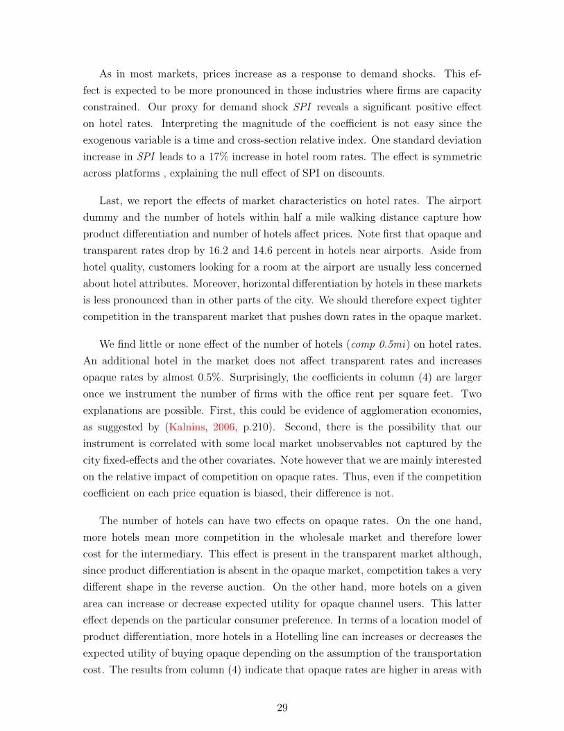
Name Your Own Price system (NYOP) and bookings made on Hotwire’s Secret Hot
Rates (SHR).6 The two platforms differ in the way buyers and the seller interact
as well as the amount of information disclosed to the buyers by the platform. The
following example helps to clarify these differences. Imagine a customer attempting
to book a hotel room on a given city-area (e.g., Downtown Los Angeles) and date.
4Courty and Liu (2013) and Fay and Laran (2009) are the only two studies that employ opaqueprices. In both cases, small samples of Hotwire’s posted prices are used. Since these data do notcontain the hotel identity associated to each opaque rate its use is limited to inferences on availabilityand price volatility over time in this specific opaque channel.
5Priceline and Hotwire are the opaque selling pioneers. They introduced their systems in 1999and 2000 respectively. Although offerings by opaque competitors have increased in recent years(Expedia and Travelocity launched opaque selling channels in 2011), they are the clear dominantplayers in the industry (“Opaque Selling in 2011” Hotel Yearbook 2011, p.96-98).
6Priceline.com has traditionally offered users the option to book in their transparent site orthrough the opaque NYOP system. More recently, Priceline added the “Express Deals” systemwhich is similar to Hotwire’s (i.e., posted prices). We only have data on Priceline’s NYOP bookingsand refer to them loosely as rooms booked on Priceline.
3

When using Hotwire.com, the consumer is presented with a list of hotels, one for
each area–stars pair, displaying room rates and hotel amenities (e.g. parking, fitness
room, free–wifi, etc). The booking process and user interface is simple and mimics
that of a transparent platform like Hotels.com. The key difference however is that
hotels names are hidden from the buyer and only revealed after the booking has been
paid.7
On the other hand, a customer using Priceline.com is asked to select the desired
room characteristics and enter her willingness to pay for it.8 The room characteristics
include check-in and check-out dates, city, hotel quality and opaque area.9 Once the
customer commits to the booking (i.e., credit card information is entered), Priceline
procures the room by running an auction among all participating hotels that match
the previously specified characteristics and notifies the customer with the booking out-
come.10 The hotel name is revealed if the transaction is successful and this happens
when a secret threshold price, in principle the winning bid plus Priceline’s commis-
sions, is below the customer’s named price. If the named price is below this threshold
price the transaction is rejected and the customer is prompted to try again with a
new bid the following day.11
It is important to highlight the differences in the booking mechanisms used by
Hotwire and Priceline. First, while room rates are posted on Hotwire’s website, buyers
using Priceline actively bid for a room. In Priceline’s system, the role of transaction
costs, impatience, expectation formation about the platform’s threshold price, and
other frictions can affect consumer sorting and the equilibrium discount. Second, in
some cases, Hotwire discloses additional information regarding the amenities of the
hotel underlying the opaque booking. It is possible that this extra information reduces
the level of opacity and therefore consumers’ uncertainty. Booking opacity levels vary
significantly across markets (e.g., a four-star booking is a different probabilistic good
if the opaque area is Manhattan’s downtown than if it is La Guardia airport). This
allows us to exploit the within-platform variation in booking discounts to estimate
the effects of opacity on consumers’ willingness to pay and relate the variation in
7The nature of opaque selling requires all bookings to be non-refundable, non-changeable andnon-transferable.
8Figures 1 and 2 in Appendix A display snapshots of Hotwire and Pricelines’s user interfaces.9The opaque areas used by Hotwire and Priceline are indistinguishable from each other. Figures
11–13 in Appendix B show some of Hotwire’s opaque areas.10Strictly speaking, Priceline and Hotwire select the hotels from their GDS (Global Distribution
Systems) with hotels’ schedules of rooms and rates available. Hotels can change their “wholesale”rates and inventory at any time making the process equivalent to a real-time auction.
11In some cases, the bidder is allowed to bid again by redefining the product category selected(i.e., the geographic area–quality pair).
4

discounts across platforms with the different features of the opaque selling format
(posted price vs. auction).
The travel industry serves two broad and very different types of customers. On
the one hand, leisure travelers are viewed as price-sensitive, with low willingness to
pay for special amenities, early demand realization and flexible schedules. On the
other hand, business travelers are naturally price-insensitive (i.e., company pays),
have strong preferences over a particular hotel (e.g., due to meetings or loyalty pro-
grams), late demand realization and high demand uncertainty (e.g., a work-related
meeting scheduled a month in advance can be canceled in the last minute). Absent the
possibility of first-degree price discrimination, hotels and airlines have traditionally
relied on revenue and yield management strategies to separate these consumers based
on the correlation of their preferences over product attributes. For example, to mini-
mize the cannibalization of sales to the business segment, leisure travelers have been
targeted with early-booking discounts and lower weekend-rates or Saturday stay-over
requirements (Talluri and Van Ryzin, 2005; Phillips, 2005).12 One natural question
we ask is whether hotels use the new opaque channels to substitute or complement
these price discrimination strategies. In other words, do consumer types fully sort by
choosing from the menu of channels or do hotels need to use within-platform pricing
strategies to achieve finer demand segmentation? This issue has not been addressed
by the existing theories of opaque selling. As we argue in Section 2, the answer de-
pends on the underlying heterogeneity in consumers’ preferences and is therefore an
empirical question.
Our findings suggest that hotels effectively use the opaque channels to price dis-
criminate consumers based on preference heterogeneity and transaction costs. Pre-
dicted opaque rates in the auction-based platform are on average 49.3% lower than
in the transparent market. Notably, the discounts for posted opaque rates are about
10 percentage points lower. The fact that both systems have survived in equilibrium
highlights the importance of selling format design and information suppression to
further segment price-sensitive customers. Opaque discounts increase monotonically
with hotels’ quality in both systems. A full star increase in hotel’s rating is associ-
ated with a 5 percentage point increase in the opaque discount. We relate this result
12These “rate feces” are based on the time of purchase and consumption. Hotels can also usephysical rate fences according to room-type attributes (view, room size, bedding type), or group-based (senior and AAA member discounts) fences (Kimes, 2002). Aside from anecdotal evidence byindustry experts and scholars, there is little work using pricing data that documents the use of thesepractices by hotels. An exception being Abrate et al. (2012) that finds evidence of inter-temporalprice discrimination by hotels in Europe, a market where opaque selling is still in its infancy.
5

to a demand-side story since product differentiation and the dispersion of consumer
valuations is expected to be larger in the higher quality segments. Interestingly,
our findings indicate that opaque bookings are not used as a last-minute resource
to dispose unsold inventory. Instead, the data is consistent with the static price-
discrimination models in the literature (Fay, 2008; Shapiro and Shi, 2008; Tappata,
2011). Moreover, the lack of evidence of within-platform price discrimination based
on check-in dates (weekends) or time of booking (early discounts) is consistent with
the notion that opaque selling channels are a substitute rather than a complement to
the traditional price discrimination strategies associated with the travel industry.
We also investigate the extent of selection on the supply side by matching each
opaque transaction to the distribution of hotel rates in the transparent market. We
find that hotels selling opaque are more likely to be those in the lower tail of the
transparent price distribution. This is consistent with anecdotal evidence from users
of Priceline and Hotwire’ systems. Both adverse selection and hotel idiosyncratic
demand shocks are hypotheses that can rationalize this pattern. The former is possible
if star-rating captures hotels’ quality imprecisely. That is, hotels with lower-than-
average quality set lower wholesale prices and are therefore selected by the opaque
platforms with a higher frequency than others. The quality differences not captured
by the discrete star-rating are expected to be long lasting and therefore reflected
in the dispersion of full-sample average prices. Alternatively, temporal idiosyncratic
shocks might have a significant impact on pricing policies. If so, a hotel’s position in
the distribution of transparent rates is likely to change from date to date according
to these shocks. When experiencing low demand, a hotel reduces its rates in all
channels and is therefore expected to outbid other hotels in the opaque platform’s
reverse auction. Our findings are consistent with the latter hypothesis. The position
in the contemporaneous distribution of transparent prices explains the probability of
selling opaque while the position in the distribution of the full-sample average prices
is not significant.
The paper is structured as follows. In Section 2 we discuss the economics of opaque
selling and discuss predictions from the theory. The empirical specification, together
with descriptions of the data and summary statistics are presented in Section 3. The
econometric results are discussed and related to existing theories of opaque selling
in Section 4. Section 5 concludes and highlights unexplored dimensions for future
research.
6

2 Industry and theoretical background
Why do hotels engage in opaque selling? The short answer is that it allows them
to segment demand and price discriminate business and leisure travelers similarly
to how airlines price discriminate using Saturday stay-over requirements or early-
booking discounts. However, there are new issues associated with opaque selling that
make the price discrimination logic more intertwined. Before discussing the literature
and economics of opaque selling, it helps to begin summarizing the main features of
the travel industry.
First, though hotels book transparent rooms directly or through “passive” OTAs,
they can only sell opaque through an active intermediary. The reason is that a third-
party is required to pool hotels and create the opaque good hence buyer uncertainty.13
Second, transparent and opaque channels coexist (sometimes offered by the same in-
termediary) and are easily accessed by customers. While the choice between buying
directly from a hotel’s website or from an OTA might be driven by buyers’ search
or switching costs, the choice between transparent and opaque bookings is primarily
driven by heterogeneity in buyers’ preferences. Third, the opaque wholesale market
operates as a “reverse auction” and it is specific to each platform. Hotels submit
their secret supply schedules (rates and number of rooms available) and the platform
chooses the winner for each marginal transaction. Market clearing in the wholesale
market is critical in determining the shape of competition in the opaque channel, its
interaction with the transparent market, and the final effect on hotels’ profits. Last,
advance purchasing is a common practice in this industry and therefore dynamic pric-
ing or revenue management considerations can impact both, transparent and opaque
pricing strategies.
Aside from quality differences, hotels differ in many horizontal dimensions and so
the demand faced by each hotel is not perfectly elastic. Selling through an opaque
channel can help a hotel to attract consumers from the lower part of the demand
curve without cannibalizing too much the sales to high-valuation consumers in the
transparent market. Consumers can vary in their intrinsic willingness to pay as well as
flexibility regarding the room characteristic: hotel brand, room usage date and room
booking date. But they can also vary in their marginal utility of income. For example,
other things equal, business travelers are expected to be less price sensitive than leisure
travelers from the basic fact that their companies pay for their trips. In addition,
13In principle, a multiproduct firm (e.g., a hotel with different room-types) could sell opaquewithout the need of an intermediary. Maybe due to the lack of commitment by a seller of verticaldifferentiated products, we do not observed this in practice.
7

they present strong preferences regarding the hotel (closest to company headquarters)
and room usage dates (weekdays). A conference or a meeting organized on a specific
hotel and date make business travelers inflexible and willing to pay significantly more
than a casual traveler that can reschedule her visit with little cost. In general, the
literature refers to those price-insensitive customers as loyal customers. A non-loyal
or shopper customer is price-sensitive and values most hotels similarly (which makes
her even more price-sensitive).
Opaque products are inferior goods and can be thought of as a special case of
damaged goods. Deneckere and McAfee (1996) and Shapiro and Varian (2000) showed
that a monopolist can increase profits and welfare by selling a “damaged” version of
the product to price-sensitive consumers. In a sense, the value destroyed by the
producer of a damaged good might allow for the creation of even more value. This
same logic underlies opaque selling. However, a key difference with the damaged good
argument is that hotels selling opaque need to do so through the opaque platform and
therefore compete aggressively for customers directly with other hotels.14 Moreover,
it is in the best interest of the platform to generate intense competition among hotels
to capture a larger margin between the wholesale cost and customers’ willingness to
pay. Nevertheless, a successful platform is required to increase the utility of some
type of customers and attract hotel participation. Low opaque prices impact hotels’
profits directly and might also attract loyal customers to the opaque platform. In
order to prevent cannibalization, price reductions in the transparent market might be
needed, depressing profits even more. In that sense–and unlike in the damaged goods
case–intense competition in the wholesale opaque market can make firms worse-off
with opaque channels than without it. That is, while opaque selling destroys value to
create more value, part of the value generated is captured by a new player. Much of
the current debate in the industry is on the impact of opaque selling on hotels’ profits.
That is, entry by an opaque intermediary can increase hotels’ profits but it is also
possible that it creates a prisoner’s dilemma making individual hotel participation
profitable but lowering aggregate profits for hotels.
The theoretical literature has focused on the conditions required for opaque sell-
ing to increase industry profits. Fay (2008) and Shapiro and Shi (2008) show that
price discrimination through opaque selling can be a successful strategy as long as
consumers are sufficiently heterogeneous or products sufficiently differentiated. In
their models, the market is segmented in equilibrium when the opaque prices attract
14By definition, hotels lose their market power in the opaque wholesale market since consumersself-selecting into the opaque channel are not willing to pay for product differences.
8

shoppers but are not low enough to attract the loyal customers.15 In these cases,
introducing opaque selling into fully-served markets increases industry profits at the
expense of consumers’ surplus. It is easy to see that opaque selling increases welfare
if it also operates in the extensive margin selling to price-sensitive customers that
would have otherwise not consumed. Tappata (2011) shows that this market expan-
sion effect is larger in markets exposed to demand seasonality where the free-entry
equilibrium leaves market gaps in the low-demand seasons.
It is important to note that the existing theories use very stylized models designed
to explain the emergence opaque selling in a given industry.16 We do not attempt to
take these models literally to the data. Instead, we use them as a basic framework to
think about opaque selling. There are two general predictions from the theory. First,
significant consumer heterogeneity is required to justify the emergence of opaque
selling. Second, conditionally on selling opaque, the difference between transparent
and opaque prices increases with product differentiation.17 A common feature from
general price discrimination models is that the price in the no-discrimination scenario
falls between the highest and lowest of the prices when the firm price discriminates.
This might not be the case with opaque selling since prices for opaque and transparent
prices can be lower than before the entry by the opaque intermediary (Tappata,
2011).18 We can not test this prediction since we do not observe hotel prices before
and after the emergence of opaque selling. Instead, we focus on the second prediction
and explore how variables that vary across markets affect the magnitude of opaque
discounts.
To fix ideas, consider a single market with j ∈ J horizontally differentiated hotels.
To isolate the effect of consumer heterogeneity on discounts, assume hotels have the
same marginal cost mc and face symmetric demands. The equilibrium transparent
and opaque rates (pτ , po) are endogenously determined with the wholesale rate (wo).
This can be summarized in a single equation. Using the Lerner index and organiz-
15Formally, Fay (2008) assumes exogenous customer loyalty in a Hotelling duopoly while Shapiroand Shi (2008) model two groups of buyers, one with low and one with high transportation costs,in a circular city.
16For tractability purposes, they only allow for few dimensions of heterogeneity among consumersand firms. Moreover, firms are not allowed to price discriminate consumers in the absence of opaqueselling. Similarly, competition between opaque platforms is not modeled.
17In the duopoly model of Fay (2008) for example, a symmetric equilibrium predicts a larger gapbetween transparent and opaque prices when consumers face larger transportation costs and theproportion of loyal customers is larger. In Tappata (2011), the gap increases with transportationcost and the distance separating firms.
18More formally, different modeling choices (e.g. exogenous vs endogenous loyalty) can lead totransparent and opaque prices being strategic substitute or complements.
9

ing terms, the opaque discount associated with hotel’s h transparent price can be
expressed as
Disch = 1− po
pτh= 1− wo
mc
[εo/(εo − 1)
ετh/(ετh − 1)
](1)
where εo and ετh represent the absolute value of the demand elasticity for opaque and
hotel h’s bookings respectively.19 Note that, since wo ≥ mc, a necessary condition for
positive discounts is εo > ετh. We now turn to the determinants of these elasticities.
Assume consumers have unit demands and their preferences are characterized by
the distribution of reservation values vj over the J transparent alternatives. Important
to the analysis of opaque selling is the entire distribution of valuations. To simplify it
even further, assume that all consumers have the same average valuation avg(vj) = v.
While the maximum valuation is relevant to choose among the transparent hotels, the
difference between this maximum and a weighted average of the J values determines
the relative preference for opaque bookings. Consumers with dispersed preferences
are expected to face significant disutility from buying opaque (i.e., max(vj)− v large).
On the other hand, consumers with fairly concentrated reservation values are likely
buyers of opaque products.20 Their expected utility from buying a lottery is not very
different from the utility obtained when booking their preferred transparent hotel.21
We illustrate the relationship between the demand for transparent and opaque
goods in Figure 1. A hotel’s market power is captured by the firm-demand elasticity
ετj which is determined by the number of hotels in the market, the extent of product
differentiation, and consumers’ price sensitivity. This is represented by the solid black
curve on Figure 1. Given a pair of transparent and opaque prices pτ and po < v, the
demand for opaque bookings faced by the platform is determined as follows. First,
hotel k’s residual demand includes all consumers for which max(vj) = vk < pτ+v−po.The residual demand is always more price-elastic than the original demand.22 Second,
the residual demand from each hotel “shifts down” to reflect the fact that opaque
goods are inferior goods relative to transparent goods. That is, the willingness to
pay for an opaque good must be discounted since consumers’ willingness to pay for
an opaque booking is associated with v instead of max(vj). The shift in the demand
is not expected to be symmetric as the disutility from opaque bookings is negatively
19In our example, hotel prices and elasticities are symmetric in equilibrium. We keep subscript hto differentiate between the firm and market demand for transparent bookings.
20In the one-dimension address models, this is represented by the interaction between consumer’sdistance to the products’ locations and transportation cost parameter.
21It is easy to see the effect of adding risk aversion on the relative demand for opaque bookings.22If q = f(p) such that there is p∗ that maximizes profits, ε = f ′(p)p/f(p). The residual demand
qR = f(p)− q∗ has elasticity εR = f ′(p)p/[f(p)− q∗] > ε.
10

correlated with consumers’ willingness to pay for the transparent booking. Last, the
J–modified–residual demands are aggregated and determine the demand for opaque
bookings (blue curve in Figure 1).23
Figure 1: Equilibrium in the Transparent and Opaque Markets
O
QdΤ
Qdo
MRo
MRΤ
T
qΤ Qoq
wo=mcpo
pΤ
$
Note: Firm-level demand and marginal revenue for transparent book-ings in black (Qτ and MRτ ). Demand for opaque bookings and marginalrevenue in blue (Qo and MRo). Wholesale price for opaque room as-sumed equal to marginal cost.
As equation 1 shows, the magnitude of the opaque discount is related to supply
and demand factors. For example, as the theory suggests, more product differenti-
ation leads to higher discounts. An increase in product differentiation is equivalent
to an increase in the dispersion of consumers’ valuations over the J available alter-
natives. That is, maxvj increases for each consumer but v remains constant. Thus,
the hotel-level demands become more elastic (higher ετ ) but the elasticity for opaque
bookings is not affected. We can also explore the different channels through which
competition affects predicted discounts. First, we expect more firms to intensify com-
petition and lower transparent prices. The impact of lower transparent prices on ετ is
translated to the residual demand (εo) and therefore discounts might not change. Sec-
ond, a change in the number of firms affects competition in the wholesale market. We
expect competition in the wholesale market to increase Disch as wo approaches mc
from above. Third, more firms can affect consumers’ valuations similarly to product
differentiation (i.e., increase maxvj for all consumers holding v constant). Other com-
parative statics can be analyzed with equation (1) and we postpone their discussion
until Section 4.
23Note that the last two steps do not affect the price-elasticity of demand.
11

The forces underlying opaque selling discussed above are present in static models
and we have so far ignored dynamic elements associated with demand uncertainty
and capacity constrained firms, two important dimensions in the travel industry. As
mentioned above, leisure travelers booking early in advance and business travelers
on dates closer to the consumption date. Exploiting the correlation between room-
booking date and willingness to pay has been the main reason for the use of revenue
management programs in the industry. However, the incentive to use dynamic pricing
might be attenuated for a hotel once it can use the opaque channel to cater price-
sensitive consumers (leisure travelers). For example, Jerath et al. (2010) present a two
period model where firms can choose to use the opaque market only in the last-minute
to sell excessive inventory. A hotel would prefer to use the competitive opaque market
in the last-minute to discounts in the transparent market if product differentiation is
large enough to keep loyal buyers away from leaking to the opaque market. Otherwise,
hotels avoid the opaque market altogether and sell excess inventory (if any) at a
discount in the transparent market. As we explain in the next section, the structure
of our data allows us to test whether opaque selling is a last-minute practice in this
industry.
3 Data and Empirical Specification
3.1 Matching opaque and transparent data
Our data contains opaque and transparent hotel room rates combined with hotel
and market characteristics. In order to describe these data, it is helpful to define
first the unit of analysis more precisely. A “booked room” j is defined by the set of
attributes {h, r, b, t} where h is the hotel identity, r the room-type (non-refundable,
standard, with view, bedding, etc), b the booking date and t the check-in date. In
other words, we define a hotel room j as the product observed by the buyer at the
time of consumption (check-in date) instead of purchase (booking date). Note that,
since opaque and transparent products only differ at the time of purchase, consumers’
information about h varies depending on whether the room was booked through the
opaque or the transparent channels. The opaque and transparent hotel rates were
obtained from different sources. We refer to them as the opaque and transparent data.
A major challenge involves the matching of each price paid in the opaque platforms
(poj) to the relevant transparent posted price (pτj ). We explain the main features of
this process in this section and leave the details to Appendix B.
The opaque data includes room bookings made on Priceline’s NYOP system and
12

Hotwire’s SHR listings. The source is the website Betterbidding.com, a forum
created to benefit users of these two popular platforms. The different sites in the
forum are designed so that users discuss strategies, share experiences and exchange
detailed information on their opaque bookings. Forum participants routinely post
the identity of the hotel, rate paid and dates when booking through Hotwire or from
a winning bid on Priceline. We have compiled and parsed these posts for the most
popular destinations in North America. We emphasize that the nature of opaque
bookings makes it impossible to obtain transaction-level information from sources
other than the opaque platforms. Though price-protection is a feature that attracts
hotels to the opaque platform, the secrecy goes beyond potential buyers and even
hotels are not aware of the rates consumers pay the opaque platforms. Self-reported
data has become available recently and this is the first study using these data to
analyze opaque pricing.
It must be noted that it is not clear whether forum participants represent the
average user of opaque platforms. On the one hand, one expects forum participant to
be frequent travelers willing to invest time and effort to obtain better-than-average
deals. On the other hand, inexperienced users are the ones most likely to seek infor-
mation and report back in these forums. This is a common issue with user-reported
data in the IO literature.24,25 In addition, there is the possibility that hotels or the
opaque platforms create fake posts in the forum to bias expectations over opaque
booking outcomes. Mayzlin et al. (2013) show that there is evidence of manipulation
of product reviews when anyone, instead of just consumers, can post them. We note
first that the benefits from faking booking rates for these firms are not as clear as in
the case of product reviews.26 Moreover, even though the cost of generating a fake
post is similar to the cost of a fake product reviews, the benefits are far lower since
forum posts get easily outdated. User accounts are required to post information on
opaque bookings. A look at the distribution of posts by user reassures us that infor-
mation manipulation is unlikely. We find that users with four or less posts represent
95% of the opaque bookings in our sample.27
24Examples of work that use self-reported data include Lewis (2008) and Dai et al. (2012). Theformer uses gasoline prices reported by drivers to GasBuddy.com and the latter uses retail store’sratings from users of Yelp.com.
25Sample bias, if any, would primarily affect Priceline’s auction-based bookings since buyer’sbidding abilities do not influence the posted offers on Hotwire.
26For example, Priceline and Hotwire both announce on their website the expected savings forconsumers. These savings are consistent with the opaque discounts in our data.
27The user with most active participation contributed with posts for 14 opaque bookings on ninedifferent hotels in NYC.
13

We paired each booked room j in the opaque data to a room rate posted in the
transparent channel. To do so, we first collected one-night transparent room rates
from Hotels.com for the largest cities in Canada and the US from October 1, 2011
to June 25, 2012.28 For each booking date b, we recorded the website’s posted rates
offered by all hotels in the city allowing for check-in dates t = {b, b + 1, ...., b + 90}.Note that this data with transparent room rates is very large and includes rates for
all room types and booking/check-in date combinations quoted by more than 5,000
hotels (i.e., about 8.1 million transparent rates per day). Such detailed data allows
us to do a proper match between opaque and transparent rates controlling for all
the attributes that define a booked room j. The rooms booked through Priceline or
Hotwire are non-refundable standard rooms. Thus, each opaque booking was matched
to the price quoted by the same hotel for its cheapest room quoted on the same check-
in date and, when possible, the same booking date. As explained in Appendix B, if
the latter condition was not met, we selected the transparent rate with closest booking
date that satisfied the other restrictions.
Figure 2: Matched bookings. Westin Bonaventure Hotel, LA
Note: Each opaque booking in the Westin Bonaventure hotel is characterized bythe triple (booking-date, check-in date and room-type). The figure displays theopaque rate paid and the transparent rate a customer would have paid if bookedthrough the transparent channel (hotels.com) on the same booking-date.
28We have also included rates from a small sample of New York City hotels from March to October2011.
14

To illustrate the rate-pairing procedure, Figure 2 displays the check-in date and
room rates (transparent and opaque) for the 37 matches made for the Westin Bonaven-
ture Hotel in Downtown Los Angeles. For example, the first pair of observations from
the left in the figure corresponds to a Priceline booking made for $80/night on Oct
3, 2011 with check-in date Oct 6. From the transparent data, we find that the rate
for “same” room was quoted at $214/night (i.e., 62% discount). The figure shows
that transparent and opaque rates set by the same hotel vary significantly as well as
the implied opaque discounts. Not shown in the figure are other sources of variation
like the opaque platform used, booking date, day of the week, and duration of stay.
To highlight the dimension of the transparent data required for the matchings in the
figure, only 37 of the 37,564 transparent rates collected for the Westin Bonaventure
Hotel in Los Angeles were used. We take advantage of the full transparent data to
create variables that capture market and competitor’s characteristics as well as to
investigate the position of hotels selling opaque on the distribution of transparent
rates. We discuss these variables and present summary statistics after describing the
econometric specifications.
3.2 Empirical specification
The main goal of this paper is to rigorously document opaque pricing and provide
answers to the following questions: What is the discount required by a consumer
that books opaquely instead of using the transparent channel? Do consumers view
posted-price and auction-based opaque selling systems as equivalent? What is the
effect of the opacity level on the willingness to pay for opaque bookings? Are opaque
bookings a last-minute practice in the industry? Do hotels price discriminate inter-
temporarily within channel? Are opaque discounts different across quality segments?
To investigate these questions we first estimate a general discount equation. We
further explore the determinants of opaque and transparent rates by analyzing pricing
equations for each channel separately. The baseline specifications are as follows:
Discj = δ0 + δ1Platform + δ2Xhr + δ3Xbt + uj (2)
ln pτj = βτ + γτXhr + ατXbt + vτj (3)
ln poj = βo + λPlatform + γoXhr + αoXbt + voj (4)
with Discj = 1− poj/pτj . The vector Xhr includes covariates associated to hotel room
and market fixed characteristics. Hotel-room attributes are hotel quality (star rating),
a dummy variables identifying hotels that belong to large chains and refundable rooms
15

sold in the transparent channel (only in equations 2 and 3).
The static market characteristics are captured by city fixed-effects and local mar-
ket metrics (e.g., number of competitors, opaque area size, dispersion of hotels’ lo-
cations, airport dummy). The number of hotels in a market influences pricing in all
channels and is potentially correlated with unobservables. We instrument the number
of firms using the office rent cost per area.29 This instrument proxies the fixed cost
faced by hotels which impacts firms’ entry/exit decisions and therefore is expected to
be correlated with the number of firms in the market. At the same time, fixed costs
do not enter in the hotels’ pricing equation. The dummy variable Platform (=1 if
Hotwire is used) captures the premium consumers place on posted-price instead of
auction-based selling systems. To summarize, the estimated coefficients δ1 and δ2 in
equation (2) inform us of the extent to which hotels use selling channels to screen
consumers based on preferences and transaction costs in a static sense.
Our data allows us to detect price and discount variation between and within
platforms. In principle, Hotels can segment their demand by setting different prices
between selling channels as well as within a selling channel. In the latter case, pricing
can differ based on the check-in date or advance booking (days between booking
and check-in dates) variables. This has been a common practice in the airline, hotel
and rental car industries to segment leisure travelers from business travelers since
the former are more likely to book earlier and on weekends. The vector Xbt include
dynamic variables that capture changes in demand composition (i.e., elasticity of the
demand curve faced by each hotel in each channel). Statistic significance of δ3 would
indicate that hotels use these within-platform segmentation practices.
We use indicators for weekend/weekday check-in dates, advance bookings and a
proxy for temporal demand shocks. Time-related demand shifts affect the hotel’s
likelihood of binding capacity constraints. A hotel’s marginal cost at booking time b
is composed by the cost of servicing a room and the opportunity cost of not selling
it at a higher price on a date closer to the check-in date t. While the former can be
assumed constant, the latter depends on the probability, at time b, of reaching full
capacity before date t. We do not observe hotels’ marginal costs. Instead, we proxy
demand fluctuations using Google Trend’s weekly measures of search popularity (SPI)
for each destination city. Unlike city fixed-effects, the SPI is a relative measure of
29Asking rent values were obtained from Jones Lang LaSalle’s (www.joneslanglasalle.com).Details on the construction of our instrumental variable and summary statistics are provided in theAppendix B.3.
16

search popularity that captures variation of popularity across cities and over time.
We describe this variable in more detail in the Appendix B.4.
3.3 Descriptive statistics
Table 1 presents the summary statistics of the variables used in the estimation of
equations 2–4.30 On average, an opaque booking allows the buyer to obtain a 44%
discount with respect to the transparent rate. The average transparent and opaque
rates are $187 and $100 dollars per night respectively. Both, opaque and transparent,
markets present significant rate dispersion. This variation is mainly influenced by
hotel quality rating and city effects (Figure 4 in Appendix A) although, as shown in
Figure 2, the rate dispersion for a given hotel can still be very large.31
Table 1: Summary Statistics
Variable Mean SD Med Min Max
Discount (%) 44.0 16.4 44.7 -37.9 90.3Transparent Rate (USD) 187 87 168 29 803Opaque Rate (USD) 100 49 90 13 380Non–refund = 1 0.30 0.46 0 0 1Platform (Hotwire = 1) 0.31 0.46 0 0 1Chain = 1 0.68 0.47 1 0 1Stars 3.73 0.65 4 2 5Weekend 0.52 0.50 1 0 1Adv Booking (weeks) 4.29 4.62 3 0 28SPI 40.98 24.30 34 3 100Airport = 1 0.11 0.32 0 0 1Area size (sqmi) 7.8 13.1 2.2 0.1 107.6Dispersion = Var(dist) 0.3 1.0 0.1 0.0 19.1Comp 1/2mi 15.0 16.3 8 0 73Hotels of = star in area 7.9 5.2 6 1 35
Bookings in our sample are twice more likely to be done on the auction-based
(Priceline) than in the posted-price (Hotwire) channel. As shown by Figure 3(a),
some of the opaque bookings have negative discounts (34 observations). Although we
do not expect opaque rates to be higher than transparent rates, we cannot discard
this event and therefore decided to keep the observations in the data.32 Hotel quality
30See Table 4 in Appendix B for the definition of each variable.31Hotel stars and city fixed effects explain 13.6% of the variance in discounts and about 45% of
the transparent and opaque rates variance.32Negative discounts are expected to be more likely in bookings through Priceline since the possi-
bility of consumer “mistakes” are larger. However, only 12 of the 34 bookings with negative discountswere done through Priceline’s channel.
17

is measured by the seven hotel star-rating levels: 2, 2.5, 3, 3.5, 4, 4.5 and 5 stars. The
average hotel quality rating is 3.7 stars and half of the transactions occurred in 4-star
and higher hotels. Although the mean quality is similar across platforms, bookings
on Priceline are more likely to be of higher quality than those on Hotwire. Moreover,
opaque bookings in general are done in hotels of higher quality than that of a random
hotel in the market (Figure 3(a) in Appendix A).
Figure 3: Discounts and early bookings distributions
(a) Opaque Discounts: (1− po/pτ ) (b) Advanced Bookings
We observe significant heterogeneity in the booking dates. The average booking is
made about 30 days in advance. The median booking is done 3 weeks in advance and
3/4 of the bookings are done within 6 weeks of the check-in date. The distribution of
advance bookings, shown in Figure 3(b), reveals that the opaque channels are open
to consumers well in advance to the check-in date. This evidence is in conflict with
the idea that the opaque channel is active only at the last minute so hotels can sell
their distressed inventory. We test whether advance bookings affect the size of the
discounts when estimating equation (2) in the next section. Motivated by Figure 5(b)
in Appendix A, we allow for non-linear effects of Advance-Booking on Discounts. The
dummy variable Weekend (stay over on Friday or Saturday night) includes the night
before a holiday in the US or Canada to capture demand from non-business travelers.
About half of the opaque transactions occur on a weekend. Figure 3(b) in Appendix
A complements this statistic with the distribution of bookings over the different days
of the week.
The Search Popularity Index (SPI ) takes values between 0 and 100 and varies
across cities and time. Figure 5(d) in Appendix A shows the SPI variability in four
18

different cities. The SPI level for a given city fluctuates significantly showing in some
cases evidence of seasonality.33 We use the dummy varables Chain and Non-refund as
controls. The former identifies hotels that belong to a large and recognizable chain.
Presumably, these hotels have more advance reservation system in place and can take
advantage of the opaque channel by dynamically updating inventory and adjusting
rates at a higher frequency than stand-alone hotels. Most of the opaque bookings
(68%) are done in hotels that belong to chains. However, this is not very different
from the proportions of chain-hotels in the population (69%).34 By definition, opaque
bookings are non-refundable and therefore should be compared to a non-refundable
transparent rate to avoid overestimation of the discounts. The transparent rates
that matched the remaining attributes of our opaque booking are more likely to be
refundable rates and only in 31% of the cases the transparent rate is non-refundable.
The variables in the bottom of Table 1 vary across markets and are associated
with product differentiation, competition and the opacity level of opaque bookings.
We calculated the walking distance between all hotels in a given city using Google
maps application and used it to determine, for each hotel, the number of hotels
within a distance threshold (Comp). We repeated this procedure for hotels of equal
(Comp same) and similar (Comp sim) star rating (plus/minus 0.5 stars). On average,
a hotel has 14 competitors within half a mile of walking distance. Four of those
competitors have the same star-rating (not reported in table). The opacity level of a
given booking is captured by the opaque area size (Area size in squared miles) and
the variance of the distance between each hotel and the weighted-centroid for the
opaque area (Dispersion). A larger variance relates to a clumped pattern of hotels.
Last, 11 percent of our observations fall in airport areas where we expect different
demand and therefore price dynamics than in the rest of the city areas.
Table 2 provides additional information regarding the dependent variables in equa-
tions 2–4. Opaque discounts are about 9 percentage points larger when opaque book-
ings are done through auction-based (Priceline) instead of posted-price system. The
variance in discounts is similar across opaque platforms and, as Figure 3(c) in Ap-
pendix A shows, this seems true for higher moments of the distribution of discounts.
33The U.S. Travel Association and American Express in their “Destination Travel Insights” providea ranking with the top 20 cities based on the number of leisure and business travelers in UnitedStates. The positions in 2013Q1 for Chicago, Las Vegas and Miami are, respectively, 4, 15, and8 in the “business destination” ranking and 3, 5, and 8 in “leisure destination” ranking (http://www.ustravel.org/research/destination-insights).
34These two numbers are not strictly comparable. It is more common that a hotel belongs to achain if it has a low star-rating. And opaque bookings are generally done in high quality hotels(thus, less likely to belong to chains).
19

Table 2: Summary Statistics–Dependent Variables
Room ratesDiscounts
Transparent Opaque %
N Mean SD Mean SD Mean SD
PlatformPriceline 2,650 190 87.85 97 47.05 46.71 15.58Hotwire 1,167 179 85.4 107 52.26 37.99 16.56
Stars
2 90 95 36.5 66 29.38 29.19 17.742.5 175 109 33.83 66 25.03 38.85 17.663 537 150 78.23 80 48.13 45.89 14.46
3.5 918 166 65.11 84.0 36.15 46.6 17.174 1,636 215 91.61 113 49.63 45.21 15.88
4.5 125 266 104.18 155 66.61 39.88 16.415 336 200 64.55 122 32.92 36.7 13.32
Chain0 1,239 194 87.59 109 50.6 41.48 16.671 2,578 183 86.91 96 47.55 45.28 16.1
Note however that the difference in mean discount might be jointly explained by
the selling system and the hotel quality segment. As we mentioned before, Hotwire
bookings are done in lower quality hotels than those on Priceline and the table shows
that discounts seem larger in the higher star-rating segment. Interestingly, the dis-
tributions of transparent and opaque rates for each star level differ beyond the first
moment.35 Figure 6(a) in the Appendix shows that transparent rates are more spread
out than opaque rates. But this is less so for lower quality hotels (2 and 2.5 stars on
Figure 6(b)). We get back to this point in the next section.
4 Results
4.1 Discount equation
We start reporting results from the estimation of equation (2). Table 3 presents four
specifications where the dependent variable (Discj ∗ 100) measures the savings by
booking in the opaque relative to the transparent channel. All specifications include
city-level fixed effects and use robust standard errors clustered at the hotel level. Our
preferred specification is given in column (4) where we instrument the competition
variable Comp 0.5mi using the office rental cost per square feet ($psf).36 Given that
35The lower hotel rates in 5-star relative to 4.5-star hotels is driven by the fact that all but oneof those hotels are located in Las Vegas, a cheaper destination than the average city in our sample.
36The number of observations in column (4) is reduced because rent data for Las Vegas andNiagara Falls are not available.
20

the estimated coefficients do not vary substantially across specification we mainly
discuss the results reported in column (4).37
The main explanatory variables affecting opaque discounts are platform used and
hotel’s quality. The coefficient for Platform shows that the 9 percentage points dif-
ference in unconditional discounts between Priceline and Hotwire (Table 2) is robust
to the inclusion of all our covariates. After accounting for non-refundability, the ex-
pected discounts are 49.2% for opaque bookings made on Priceline and 39.5% for
opaque bookings made on Hotwire. Given the supply-side similarities of these two
platforms, we attribute the sign and magnitude of the Platform coefficient to the
frictions involved in the NYOP bidding system. In particular, the transaction costs
imposed to buyers due to the multiple bidding restrictions. Note however that this
represents an upper bound of the effect of auction-based, instead of posted-price sell-
ing systems. The differences in discounts could also be attributed to the sometimes
lower uncertainty faced by Hotwire’s users. A hotel room is a bundle of attributes
each valued differently by consumers. Some have strong preferences over specific
hotel location within the opaque area, others on the amenities available, and other
consumers might just care about the hotel identity (e.g., to obtain loyalty rewards).
Conditional on buying opaque, and Hotwire releasing more information about the
opaque hotel than Priceline (e.g., swimming pool availability), the expected util-
ity for these consumers would be higher if buying through Hotwire. The reason is
that buyers can update their—uniform—prior probabilities attached to each hotel in
a given opaque area.38 We argue that the information component of the discount
spread across platforms is unlikely to be large. First, as can be observed from Figures
1 and 2 in Appendix A, only in few instances the information regarding an opaque
hotel’s amenities are different from those expected from a hotel of a given star-rating.
Second, as we show below, the opacity level has little effect on the size of the observed
discounts.
Better deals are obtained when booking higher quality hotels. Discounts increase
on average by 6.62 percentage points for each full unit increase in Stars.39 The box-
plot in Figure 4 shows the monotonic relation between predicted discounts, hotel star-
rating and selling platform. Hotel rates in each channel are bounded by consumers’
willingness to pay and the marginal cost of providing a room with the exact level
37We fail to reject the null hypothesis of exogenous Comp 0.5mi.38Note that the logic is conditional on buying opaque. Buyers with strong preferences over a
hotel’s amenity would most likely use the transparent channel.39This result is similar across platforms and robust to other non-linear specifications (e.g., star
level dummies).
21

Table 3: Discount RegressionsDependent variable: Discj ∗ 100
(1) (2) (3) (4)Platform (Hotwire=1) -8.619*** -8.679*** -8.645*** -9.328***
(0.694) (0.688) (0.678) (0.726)Non–refund -2.814*** -1.688 -1.714 -1.340
(0.839) (0.990) (0.948) (0.934)Chain 0.782 0.888 0.614 0.865
(1.369) (1.390) (1.365) (1.192)Stars 3.107*** 3.598*** 3.588*** 5.285***
(0.857) (1.022) (1.067) (1.218)Airport = 1 2.595 2.529 1.564 1.908
(1.451) (1.465) (1.421) (1.409)Weekend 0.151 0.303 2.413
(3.308) (3.262) (3.994)Wknd*Stars -0.695 -0.746 -1.498
(0.854) (0.844) (1.073)Adv Booking (wks) -0.426** -0.387* -0.282
(0.159) (0.158) (0.167)AdvBook2 0.025*** 0.023*** 0.021**
(0.007) (0.007) (0.008)NonRef*AdvBook -0.213 -0.217 -0.285*
(0.131) (0.128) (0.129)SPI 0.077 0.076 0.013
(0.042) (0.042) (0.047)Area size (sqmi) 0.081* 0.081*
(0.037) (0.038)Dispersion=Var(distance) -1.473*** -1.119**
(0.417) (0.355)Comp 0.5mi -0.075* -0.130
(0.036) (0.090)Constant 43.480*** 41.490*** 42.616*** 38.159***
(3.588) (4.239) (4.498) (4.862)City fixed effects Yes Yes Yes YesR-squared 0.194 0.205 0.213 0.222N 3817 3817 3817 3180Underidentification:Kleibergen-Paap rk LM statistic 28.426Chi-sq (p-val) 0.000
Weak identification:Kleibergen-Paap rk Wald F statistic 63.592
Robust standard errors clustered at the hotel level in parenthesis. *** p < 0.01, ** p < 0.05, * p < 0.1.2-step GMM with Comp 5mi instrumented in Column (4).
22

being determined by competition in the marketplace. Naturally, all else equal, these
bounds increase with a hotel’s quality explaining why transparent and opaque rates
increase with star ratings. We find that quality affects transparent rates more than
opaque rates and this is consistent with the combination of some of the following
elements: (i) strong competition in the wholesale opaque markets, (ii) demand for
transparent products in the low quality segment is more elastic than in the high
quality, (iii) the demand for opaque products in the high quality segment is more
elastic than in the low quality segment. The first is intuitive since the reverse auction
implemented by the opaque platform removes product differentiation and therefore,
delivers a low wholesale cost to the platform.40 Note however that condition (i) alone
is not sufficient to explain the larger discounts for higher quality hotels observed in
the data. Aside from the wholesale cost of the opaque room, the intermediary must
face a more elastic demand in the opaque market for hotels with higher star-rating.
This could be due to the fact that consumers in the high quality segment have more
dispersed preferences than those in the low quality segment. This leads to a more
inelastic demand in the tranparent segment and higher elasticity in the opaque market
since consumers’ valuations for opaque goods become less dispersed. Moreover, as the
constant gap across platforms in the figure suggests, the effect described above does
not seem to be asymmetric among consumers with different transaction costs.41 On
a side note, it is interesting that Priceline provides their customers the city-area and
star-level where best deals can be obtained. Consistent with our findings, the “best
deals” recommend ed for the bookings in our database are 66% of the time for 4-star
hotels and only 0.02% of the time for a 2-star hotel.
Notably, the remaining coefficients in Table 3 are either insignificant or have a very
small economic impact on opaque discounts. First, discounts by hotels associated to
large chains are not different from those at other hotels. Although the definition
used for Chain is somewhat subjective, the results do not change when alternative
definitions are used (e.g., the ten largest chains in the industry only). Second, it
appears that the traditional price discrimination practices in the travel industry, if
any, are not different in the transparent and opaque markets. Discounts on check-
in dates associated with demand driven by leisure travelers are not different than
discounts on other dates. The estimated coefficient for the Weekend is positive yet
not statistically significantly different from zero. The insignificant coefficient for the
interaction term between the variables Weekend and Stars grants that we are not
40In a truly Bertrand Paradox environment the wholesale cost equals the hotel marginal cost.41We estimated equation 2 including the interaction term between Platform and Stars and found
the coefficient insignificant (not reported and available upon request).
23

Figure 4: Predicted Opaque and Semi-Opaque Discounts
masking a situation where high and low star-rated hotels have inverse pricing policies
regarding weekend and weekdays.
More importantly, discounts are weakly affected by advanced bookings. The point
estimates suggest a non-linear relationship where, relative to last-minute booking, the
opaque discounts are larger if booked more than 13.5 weeks in advance. The worst
time to book opaque being around seven weeks in advance (-0.78 percentage points).
However, only the quadratic term is significant at the 10 percent level suggesting
that the median booking (three weeks in advance) obtains a discount that is only
0.15 percentage points higher than a last-minute booking.42 This result, combined
with the null effect of demand shocks (SPI ) on opaque discounts and the fact that
the average opaque bookings occurs 4 weeks in advance of the check-in date (Figure
3 and Table 2), supports the static price discrimination theories described in Section
2 and rejects the notion that hotels use opaque channels as a last minute resource to
dispose of their unsold inventory.
Surprisingly, the size of the opaque area on discounts is not statistically significant
in column (4). As expected, the coefficient is positive meaning that consumers require
larger discounts for bookings that have higher opacity level. But this effect is small:
42The quadratic term used in the specification captures most of the non-linear effects of AdvancedBooking on Discounts. Figure 7 in Appendix A shows that the residuals from the regression incolumn (4) are indistinguishable from each other.
24

a one standard deviation increase in Area size leads to only one tenth of a percentage
point increase in opaque discounts. We find discounts to be about 0.8 percentage
points lower in areas where hotels are one standard deviation more “dispersed”. Note
that, our dispersion variable measures the variance in hotels’ distances to the area
centroid. That is, more dispersion means that the spatial distribution of hotels is
asymmetric allowing for the possibility of local clusters. Last, discounts are not
influenced by the number of firms in the market nor whether the hotel is located in an
airport. We note that these results do not mean that the covariates have insignificant
economic impact in the equilibrium of the transparent and opaque markets. The
observed discounts might mask symmetric impact of these variables in each market.
We return to this when present the pricing equation results.
The main takeaway from Table 3 is that the discounts offered by hotels fit the
predictions from the simple (static) mechanisms of demand segmentation when con-
sumers have heterogeneous preferences among product attributes. As expected, cus-
tomers booking in opaque markets obtain substantial discounts in exchange for not
observing information about their service providers. The discounts in the posted-
price platform are lower than in the auction-based platform and reflect the role of
transaction costs in segmenting further opaque users. Regardless of platform, opaque
discounts increase monotonically with hotel star-rating. Last, the evidence supports
the idea that opaque bookings are a tool for price discrimination that is used reg-
ularly by hotels and not as a last-minute resource. We now turn to the analysis of
the pricing equations to get a better understanding of the mechanisms underlying the
discounts results.
4.2 Price equations
We now present the results from estimating the pricing equations (3) and (4). Tables
4 and 5 show, for transparent and opaque rates respectively, similar specifications
to the ones used when estimated the discount equation. As before, we focus on
results reported on column (4) and analyze the estimated coefficients for opaque and
transparent rates jointly.
As expected, the major impact on hotel transparent rates—together with destina-
tion city—is given by hotels’ star rating. Transparent room rates increase by about
44% (exp(0.369) − 1) with each additional star in a hotel’s quality rating. To put
this magnitude in perspective, the largest city fixed effect (Washington, DC) shifts
transparent rates by 39% relative to the baseline—and cheapest—city (Atlanta). Con-
25

Table 4: Price Regressions. Transparent BookingsDependent variable: ln pτj
(1) (2) (3) (4)Non–refund -0.094*** -0.102*** -0.101*** -0.093***
(0.019) (0.022) (0.022) (0.023)Chain 0.023 0.031 0.033 0.032
(0.029) (0.028) (0.029) (0.028)Stars 0.358*** 0.348*** 0.342*** 0.350***
(0.022) (0.023) (0.024) (0.024)Airport = 1 -0.176*** -0.176*** -0.161*** -0.164***
(0.033) (0.033) (0.032) (0.031)Weekend -0.185* -0.179* 0.004
(0.085) (0.085) (0.079)Wknd*Stars 0.039 0.037 -0.026
(0.023) (0.024) (0.022)Adv Booking (wks) 0.007 0.006 0.009*
(0.004) (0.004) (0.004)AdvBook2 -0.000 -0.000 -0.000
(0.000) (0.000) (0.000)NonRef*AdvBook 0.001 0.000 -0.002
(0.003) (0.003) (0.003)SPI 0.007*** 0.007*** 0.008***
(0.001) (0.001) (0.001)Comp 0.5mi 0.002 0.003
(0.001) (0.002)Constant 3.614*** 3.510*** 3.512*** 3.456***
(0.086) (0.095) (0.094) (0.092)City fixed effects Yes Yes Yes YesR-squared 0.506 0.522 0.525 0.554N 3817 3817 3817 3180Underidentification:Kleibergen-Paap rk LM statistic 34.659Chi-sq (p-val) 0.000
Weak identification:Kleibergen-Paap rk Wald F statistic 77.546
Robust standard errors clustered at the hotel level in parenthesis. *** p < 0.01, ** p < 0.05, *p < 0.1. 2-step GMM with Comp 5mi instrumented in Column (4).
26

sistent with the monotonic relationship between stars and discounts discussed above,
opaque rates increase by only 26.5% with hotel’s quality.43 Similarly, the Platform
coefficient on Table 5 shows that opaque rooms are 16% more expensive when booked
using Hotwire’s posted-price system rather than bidding on Priceline’s NYOP system.
The price premium for a refundable room is about 10% (Table 4). Refundable
rooms offer buyers in the transparent market the opportunity to cancel a booking at
no cost before the check-in date. In principle, the premium for refundable rooms in
competitive markets reflects this option-value to consumers and therefore converges
to zero as the booking date approaches the check-in date (i.e., as consumers’ uncer-
tainty is resolved). Interestingly, we do not observe such convergence: the coefficient
for the interaction term between Non-refund and Adv Booking is not significantly
different from zero (as in Table 3). This result is consistent with the use of refund-
able and non-refundable pricing options to screen consumers and exploit frictions in
the transparent market.44 For example, imagine that a subset of business-travelers
(high valuations and high demand uncertainty) are required by their companies to
always buy refundable hotel rooms. In this extreme case, hotels might choose to set
the refundable premium constant over time to extract surplus from this subset of
customers.45
Anticipating a booking by one week is associated with higher transparent and
opaque rates (0.9 and 1.2 percent respectively). As Figure 5 in Appendix A shows,
hotel rates patterns behave similarly as the booking date approaches the check-in
date. The symmetric effect of early bookings explains the small effect of Adv Book-
ing on opaque discounts. We link the positive and symmetric estimated coefficients
for AdvBook to traditional peak-load pricing strategies that are not related to de-
mand segmentation. Again, we do not find evidence of price discrimination based
on weekend/weekday check-in dates. This is somewhat a surprising result since it is
commonly assumed to be an important dimension exploited by the travel industry
to segment leisure and business travelers. As we argued before, it is quite possible
that hotels do not need to price discriminate within each platform if the existence of
opaque channels allows the screening of such consumers.
43As with the discount equation estimation, we found no evidence of non-linear effects of star-ratings on transparent or opaque prices.
44Escobari and Jindapon (2012) present a model that introduces the possibility of price discrim-ination through refundable and non-refundable rates. They also show that refundable and non-refundable airfares converge over time. Watanabe and Moon (2013) link refundable premiums andprice discrimination in the airline industry exploiting cross-section variation across markets.
45Alternative, assume that demand uncertainty and consumer’s willingness to pay are positivelycorrelated and, that consumers’ uncertainty is constant and only resolved at the very last minute.
27

Table 5: Price Regressions. Opaque BookingsDependent variable: ln poj
(1) (2) (3) (4)Platform (Hotwire=1) 0.135*** 0.128*** 0.126*** 0.145***
(0.017) (0.016) (0.016) (0.016)Chain -0.002 0.001 0.005 0.000
(0.024) (0.023) (0.022) (0.024)Stars 0.301*** 0.282*** 0.266*** 0.239***
(0.024) (0.026) (0.027) (0.029)Airport = 1 -0.235*** -0.234*** -0.195*** -0.211***
(0.030) (0.030) (0.029) (0.030)Weekend -0.172* -0.165* -0.012
(0.076) (0.076) (0.081)Wknd*Stars 0.049* 0.048* -0.004
(0.021) (0.021) (0.022)Adv Booking (wks) 0.015*** 0.013*** 0.015***
(0.003) (0.003) (0.003)AdvBook2 -0.001*** -0.000*** -0.001**
(0.000) (0.000) (0.000)SPI 0.005*** 0.005*** 0.008***
(0.001) (0.001) (0.001)Area size (sqmi) -0.002** -0.002
(0.001) (0.001)Dispersion=Var(distance) 0.012 -0.003
(0.011) (0.011)Comp 0.5mi 0.003*** 0.005**
(0.001) (0.002)Constant 2.999*** 2.924*** 2.959*** 3.000***
(0.088) (0.101) (0.107) (0.118)City fixed effects Yes Yes Yes YesR-squared 0.570 0.582 0.595 0.643N 3817 3817 3817 3180Underidentification:Kleibergen-Paap rk LM statistic 28.109Chi-sq (p-val) 0.000
Weak identification:Kleibergen-Paap rk Wald F statistic 63.073
Robust standard errors clustered at the hotel level in parenthesis. *** p < 0.01, ** p < 0.05, *p < 0.1. 2-step GMM with Comp 5mi instrumented in Column (4).
28
As in most markets, prices increase as a response to demand shocks. This ef-
fect is expected to be more pronounced in those industries where firms are capacity
constrained. Our proxy for demand shock SPI reveals a significant positive effect
on hotel rates. Interpreting the magnitude of the coefficient is not easy since the
exogenous variable is a time and cross-section relative index. One standard deviation
increase in SPI leads to a 17% increase in hotel room rates. The effect is symmetric
across platforms , explaining the null effect of SPI on discounts.
Last, we report the effects of market characteristics on hotel rates. The airport
dummy and the number of hotels within half a mile walking distance capture how
product differentiation and number of hotels affect prices. Note first that opaque and
transparent rates drop by 16.2 and 14.6 percent in hotels near airports. Aside from
hotel quality, customers looking for a room at the airport are usually less concerned
about hotel attributes. Moreover, horizontal differentiation by hotels in these markets
is less pronounced than in other parts of the city. We should therefore expect tighter
competition in the transparent market that pushes down rates in the opaque market.
We find little or none effect of the number of hotels (comp 0.5mi) on hotel rates.
An additional hotel in the market does not affect transparent rates and increases
opaque rates by almost 0.5%. Surprisingly, the coefficients in column (4) are larger
once we instrument the number of firms with the office rent per square feet. Two
explanations are possible. First, this could be evidence of agglomeration economies,
as suggested by (Kalnins, 2006, p.210). Second, there is the possibility that our
instrument is correlated with some local market unobservables not captured by the
city fixed-effects and the other covariates. Note however that we are mainly interested
on the relative impact of competition on opaque rates. Thus, even if the competition
coefficient on each price equation is biased, their difference is not.
The number of hotels can have two effects on opaque rates. On the one hand,
more hotels mean more competition in the wholesale market and therefore lower
cost for the intermediary. This effect is present in the transparent market although,
since product differentiation is absent in the opaque market, competition takes a very
different shape in the reverse auction. On the other hand, more hotels on a given
area can increase or decrease expected utility for opaque channel users. This latter
effect depends on the particular consumer preference. In terms of a location model of
product differentiation, more hotels in a Hotelling line can increases or decreases the
expected utility of buying opaque depending on the assumption of the transportation
cost. The results from column (4) indicate that opaque rates are higher in areas with
29

more hotels. The coefficient is very small and therefore not significantly different from
zero in the estimation of the discount equation. The variables associated with opacity
level (area size and dispersion) in Table 5 are not significant and present a puzzle to
our theoretical predictions. More importantly, we would expect bookings in larger
opaque areas to be associated with more uncertainty and therefore a lower opaque
price. Taken together, our findings suggest that consumers require a large discount
to be willing to buy a lottery instead of a known product. However, conditional on
buying opaque, these consumers are not very sensitive to the opacity level. In other
words, variables that affect the distribution of probabilities over the likely outcomes
do not change consumers’ willingness to pay.
4.3 Who sells opaque?
We argued above that observed hotel rates induce heterogeneous consumers to self-
select across selling channels based on their preferences and transaction costs. We now
examine the extent of hotel selection in the opaque channels. A common belief among
users of opaque platforms is that, given the area-quality selected, a buyer is more likely
to be assigned to a lower-than-average quality hotel. That is, the underlying lottery
in an opaque booking encompasses non-uniform probabilities “biased” toward inferior
hotels. On the other hand, it can be argued that hotels using the opaque market to
segment demand will increase their prices in the transparent market relative to those
that are not using the opaque channel Fay (2008). In other words, we should expect
that conditionally on selling in the opaque market, a hotel will charge a higher price in
the transparent market. We can test these hypothesis since, for each opaque booking,
we also observe the transparent rates posted by all hotels of similar quality in the
relevant opaque area. More generally, we use this information from the transparent
market to study the characteristics of the hotels that sell opaque.
In principle, each opaque booking involves a reverse auction in the back-end among
all hotels that satisfy a customer’s request (opaque area and hotel quality) where
only the winning hotel is disclosed to the buyer. That is, for each opaque transaction
i = {1, 2, ..., N} in our data, we expect the opaque platform to select the hotel willing
to rent a room at the lowest rate. Let
Bij = −αi − bij = −αi − (xijβ + vj)
represent the rate submitted by hotel j to serve buyer i where αi represents market-
specific shock and xij captures a hotel’s opportunity cost of selling a room in future
30

dates and alternative selling channels. That is, a hotel that does not expect to be
capacity constrained by the check-in date is more likely to submit a lower bid to
the opaque platform. On the other hand, a hotel close to capacity faces a higher
opportunity cost and would be willing to sell opaque only if compensated accordingly
(higher Bij). Market wide shocks to demand or supply should only alter the level of
the bids while hotel specific shocks are relevant to identify the auction winner. We use
different covariates that proxy the value of a room opportunity cost for each hotel at
a given point in time. Additionally, we assume that unobservables vj are drawn from
a Type I extreme value distribution. The probability that hotel h ∈ Ji is selected by
the opaque intermediary is therefore given by
Pr(yih = 1) = Pr(Bih < Bij) = Pr(bih > bij) =exp(xihβ)∑Jij=1 exp(xijβ)
. (5)
We estimate this probability with a conditional logit regression can be estimated
using conditional logit (McFadden, 1974) using different specifications. To illustrate
the data used and the variation in our covariates we show in Figure 5 a snapshot
of four opaque bookings made with 3.5-star hotels in Downtown Los Angeles. For
each booking, the figure displays the opaque rate and channel used together with
the transparent rates set by all hotels in the market. Hotels’ ids are also displayed
and they match the within-market ranking of hotels based on the average price in
the full-sample (1=lowest price). For example, the opaque booking with check-in
date 10/28/2011 is one of the bookings supplied by The Westin Bonaventure Hotel
displayed in Figure 2. The Westin hotel ranks fifth among the eight 3.5-star hotels in
Downtown Los Angeles. However, its price for a night on October 28th was relatively
cheaper (third).46
Controlling for opaque area and star-rating, a hotel ranking based on the full-
sample average price reflects within-market variation in quality that is not captured
by the discrete star-rating system. Moreover, rankings based on the prices charged by
competitors in a given date reflect both, quality differences and the hotel idiosyncratic
opportunity cost for a room. The four cases in Figure 2 reveal general patterns present
in the data. First, price dispersion varies over time. Second, hotels’ price-ordering is
not constant although some correlation with the full-sample ranking is present. These
two effects combined suggest that hotels experience significant idiosyncratic shocks
46As with the matching of transparent and opaque rates in the previous section, the booking date,length of stay and room type is also controlled for.
31

in demand. Last, the transparent rate charge by the opaque booking provider can be
located anywhere in the distribution of transparent prices.
Figure 5: Data snapshotFour examples from 3.5 star hotels in Downtown–Los Angeles
Note: The cases displayed are a subset of the 41 opaque bookings made by3.5 star hotels in the Downtown–Los Angeles opaque area. For each opaquebooking, the opaque and transparent rates are displayed together with hotels’ idwhich matches the overall price-ranking in our database (1 = lowest price). Forexample, the first opaque booking (check-in date: Oct 28, 2011) was done by theWestin Bonaventure, a hotel that in our dataset ranks 5th among the eight 3.5star hotels in Downtown–LA.
Results for markets with 4 to 9 competitors are reported in Table 6. Column (1)
shows how hotel h’s current rank in the transparent market (1=cheapest rate) impacts
the probability of selling opaque. The coefficients are expressed relative to the baseline
category (Rankt = 1) and, except for the case of Rankt = 2, hotels charging higher
transparent rates are less likely to be the providers of the opaque booking. Columns
(2) and (3) show a similar picture if we estimate equation 4.3 separately for Hotwire
and Priceline. In column (4), we include the full-sample ranking as a covariate to
control for the within market variance in quality. The coefficient is significant and
positive indicating that hotels of higher quality (i.e., higher average prices) are more
likely to sell in the opaque market. Note that the coefficients for the Rankt remain
similar to those in column (1). That is, it is more likely that the hotel assigned in an
opaque booking is currently renting rooms at a low price in the transparent market.
However, the low transparent rates are due to temporal idiosyncratic shocks and not
32

associated with a hotel being of lower-than-average quality.
The ranking variables Rankt and Rank aggregate information related to the cur-
rent and average prices by hotels in a given market. These are discrete variables that
do not reflect the size of price differences between hotels. Moreover, since our markets
vary from 4 to 9 hotels, the domain for each variable differs across markets and the
results in columns (1)-(4) might mask some relationships that are present in large
markets but not in markets with few hotels. In column (6) we introduce continuous
variables that normalize ranking and prices in the zero-one interval. The variables
RRj and RRjt takes a value of zero and one if the corresponding price ranking for
hotel j is one or Ji. Similarly, we define RPjt = (pτjt − pτi )/(pτi − pτi ) where pτ
iand pτi
are the lowest and highest transparent rates associated with a given opaque booking
i. While RRjt can only take equidistant values, RPjt can take any value in the unit
line. Results in Column (5) indicate that, holding constant the absolute price rank-
ings, a higher “relative price” reduces the probability of selling opaque further. Last,
the specification in column (6) incorporates the three normalized variables reflecting
relative rankings and prices. While all coefficients preserve the signs consistent with
the results in previous specifications, only the coefficient for RRt is significant.
The main message from Table 6 is that the current transparent rate charged by
a hotel in a given quality-area market is a good predictor of the probability of such
hotel serving an opaque booking. Hotels facing a low opportunity cost for a room (low
demand relative to capacity) sell at cheaper rates in all channels. Thus, the likelihood
of winning the reverse auction implemented by the opaque platform increases. We
also reject the idea that hotels that underprice competitors systematically are more
likely to sell opaque. We interpret these results as partially reconciling the theories
that emphasize the role of the opaque channel to sell unsold inventory with those
that identify the price discrimination role. On any given date (e.g., three weeks
before check-in) a hotel might find that the current inventory is above the expected
threshold. As a consequence it lowers rates across the board and chances of selling
opaque increase. The main difference with the prediction from Jerath et al. (2010) is
that the hotel does not wait until the last minute to do so.
5 Conclusions
We used a unique dataset with opaque transactions to document stylized facts and
provide insights on the economics of opaque selling. Our results are consistent with ho-
tels using selling channels to segment their demand based on consumers’ preferences
33

Table 6: Conditional Logit EstimatesDependent variable: Pr(sell opaque) = Pr(yih = 1)
Hotwire Priceline(1) (2) (3) (4) (5) (6)
Rankt :=2 -0.015 -0.049 0.000 -0.038
(0.065) (0.118) (0.078) (0.065)=3 -0.232*** -0.336** -0.188* -0.275***
(0.069) (0.128) (0.082) (0.070)=4 -0.455*** -0.513*** -0.430*** -0.525***
(0.073) (0.135) (0.087) (0.078)=5 -0.608*** -0.557*** -0.636*** -0.707***
(0.090) (0.154) (0.110) (0.098)=6 -0.808*** -0.816*** -0.807*** -0.923***
(0.117) (0.201) (0.144) (0.124)=7 -0.928*** -1.291*** -0.784*** -1.084***
(0.142) (0.285) (0.164) (0.154)=8 -0.714*** -1.645*** -0.466* -0.883***
(0.171) (0.462) (0.186) (0.179)=9 -1.042** -1.487* -0.822 -1.226**
(0.392) (0.727) (0.467) (0.396)Rankt -0.112***
(0.027)Rank 0.045** 0.048***
(0.014) (0.014)RPt -0.393** -0.233
(0.124) (0.163)RRt -0.642***
(0.169)RR 0.147*
(0.073)N 11805 3551 8254 11805 11801 11801Log-L value -3404.94 -1006.36 -2393.20 -3400.44 -3399.58 -3402.56Pseudo R2 0.022 0.032 0.019 0.023 0.023 0.022
Robust standard errors clustered at the market level in parenthesis. *** p < 0.01, ** p < 0.05, *p < 0.1. Rank = 1 if a hotel has the lowest full-sample average transparent price in a given market(area and star rating). RR = (Rank−1)/(Ji−1) ∈ [0, 1] is the normalized rank. RRt = normalizedprice-ranking in the transparent market for a given check-in date t. RPt = normalized price forcheck-in date t.
34

over hotel attributes and transaction costs. Demand shocks and advance booking
affect pricing strategies symmetrically across platforms suggesting that opaque inter-
mediaries are not used as a last minute resource by hotels. Moreover, there is little
evidence of price discrimination within a platform. This is consistent with opaque
platforms fully segmenting consumer types and leaving no room for within-platform
price discrimination.
35

References
Abrate, G., Fraquelli, G. and Viglia, G. (2012). Dynamic pricing strategies: Evidence
from european hotels, International Journal of Hospitality Management 31(1): 160–
168.
Courty, P. and Liu, W. (2013). Opaque selling: Static or inter-temporal price dis-
crimination?, Working Paper .
Dai, W., Jin, G. Z., Lee, J. and Luca, M. (2012). Optimal aggregation of consumer
ratings: An application to yelp.com, Working Paper 18567, National Bureau of
Economic Research.
URL: http://www.nber.org/papers/w18567
Deneckere, R. J. and McAfee, R. P. (1996). Damaged goods, Journal of Economics
and Management Strategy 5(2): 149174.
Escobari, D. and Jindapon, P. (2012). Price discrimination through refund contracts
in airlines, Working Paper .
Fay, S. (2008). Selling an opaque product through an intermediary: The case of
disguising ones product, Journal of Retailing 84(1): 59–75.
Fay, S. and Laran, J. (2009). Implications of expected changes in the seller’s price in
name-your-own-price auctions, Management Science 55(11): 1783–1796.
Goldmanis, M., Hortasu, A., Syverson, C. and Emre, n. (2010). E-commerce and the
market structure of retail industries*, The Economic Journal 120(545): 651–682.
URL: http://dx.doi.org/10.1111/j.1468-0297.2009.02310.x
HSMAI Foundation (2012). Distribution channel analysis. a guide for hotels.
URL: http://www.hsmai.org
Jerath, K., Netessine, S. and Veeraraghavan, S. K. (2010). Revenue management with
strategic customers: Last-minute selling and opaque selling, Management Science
56(3): 430–448.
Kalnins, A. (2006). Markets: The us lodging industry, The Journal of Economic
Perspectives 20(4): 203–3A.
Kimes, S. E. (2002). A retrospective commentary on discounting in the hotel indus-
try: A new approach, The Cornell Hotel and Restaurant Administration Quarterly
43(4): 92–93.
36

Lewis, M. (2008). Price dispersion and competition with differentiated sellers*, The
Journal of Industrial Economics 56(3): 654–678.
URL: http://dx.doi.org/10.1111/j.1467-6451.2008.00348.x
Mayzlin, D., Dover, Y. and Chevalier, J. A. (2013). Promotional reviews: An empir-
ical investigation of online review manipulation, The American Economic Review
forthcoming.
Phillips, R. (2005). Pricing and revenue optimization, Stanford Business Books.
Shapiro, C. and Varian, H. R. (2000). Versioning: The smart way to sell information,
Harvard Business Review 76(6): 10614.
Shapiro, D. and Shi, X. (2008). Market segmentation: The role of opaque travel
agencies, Journal of Economics & Management Strategy 17(4): 803–837.
Talluri, K. T. and Van Ryzin, G. J. (2005). The theory and practice of revenue
management, Vol. 68, Springerverlag Us.
Tappata, M. (2011). Strategic vertical market structure with opaque products, Work-
ing Paper .
Watanabe, M. and Moon, S. (2013). Refundability and price: Empirical analysis on
the airline industry, Available at SSRN 1681337 .
37
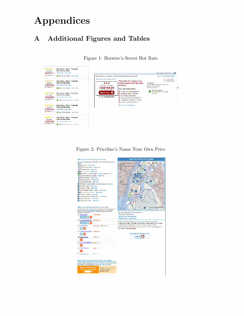
Appendices
A Additional Figures and Tables
Figure 1: Hotwire’s Secret Hot Rate
Figure 2: Priceline’s Name Your Own Price
1

Figure 3: Descriptive Statistics
(a) Quality distribution: opaque bookings and hotels (b) Check-in day of the week
(c) Discounts distribution by platform (d) Search Popularity Index
2

Figure 4: Opaque discounts and hotel rates by city
Figure 5: Opaque discounts and hotel rates dynamics
(a) Rates (b) Discounts
Figure 6: Opaque and transparent room rate densities
(a) All observations (b) Hotels with stars < 3
3

Table 1: Price Regressions by PlatformDependent variables: ln pτj and ln poj
All Hotwire Pricelineln pτj ln poj ln pτj ln poj ln pτj ln poj(1) (2) (3) (4) (5) (6)
Non–refund -0.093*** -0.085* -0.096***(0.023) (0.033) (0.026)
Platform (Hotwire=1) 0.145***(0.016)
Chain 0.032 0.000 0.054 0.002 0.009 -0.008(0.028) (0.024) (0.037) (0.030) (0.032) (0.028)
Stars 0.350*** 0.239*** 0.352*** 0.247*** 0.337*** 0.234***(0.024) (0.029) (0.035) (0.038) (0.031) (0.037)
Airport = 1 -0.164*** -0.211*** -0.129** -0.215*** -0.184*** -0.208***(0.031) (0.030) (0.044) (0.040) (0.034) (0.033)
Weekend 0.004 -0.012 -0.032 -0.085 0.006 0.046(0.079) (0.081) (0.127) (0.119) (0.099) (0.103)
Wknd*Stars -0.026 -0.004 -0.018 0.006 -0.026 -0.016(0.022) (0.022) (0.036) (0.034) (0.027) (0.028)
Adv Booking (wks) 0.009* 0.015*** 0.007 0.009 0.012* 0.016***(0.004) (0.003) (0.006) (0.005) (0.005) (0.004)
AdvBook2 -0.000 -0.001** -0.000 -0.000 -0.000 -0.001*(0.000) (0.000) (0.000) (0.000) (0.000) (0.000)
NonRef*AdvBook -0.002 -0.002 -0.003(0.003) (0.004) (0.003)
SPI 0.008*** 0.008*** 0.008*** 0.008*** 0.008*** 0.008***(0.001) (0.001) (0.002) (0.002) (0.001) (0.001)
Area size (sqmi) -0.002 0.001 -0.003**(0.001) (0.001) (0.001)
Dispersion=Var(distance) -0.003 -0.026 0.006(0.011) (0.021) (0.011)
Comp 0.5mi 0.003 0.005** 0.007*** 0.006** 0.000 0.004(0.002) (0.002) (0.002) (0.002) (0.002) (0.002)
Constant 3.456*** 3.000*** 3.415*** 3.134*** 3.529*** 3.020***(0.092) (0.118) (0.152) (0.163) (0.111) (0.147)
City fixed effects Yes Yes Yes Yes Yes YesR-squared 0.554 0.643 0.563 0.612 0.547 0.659N 3180 3180 977 977 2203 2203Underidentification:Kleibergen-Paap rk LM statistic 34.659 28.109 31.241 26.157 23.866 18.725Chi-sq (p-val) 0.000 0.000 0.000 0.000 0.000 0.000
Weak identification:Kleibergen-Paap rk Wald F statistic 77.546 63.073 69.979 55.230 61.759 48.000
2-step GMM with Comp 5mi instrumented in all columns. Robust standard errors clustered at the hotel level in parenthesis.*** p < 0.01, ** p < 0.05, * p < 0.1.
4

Table 2: Price Regressions by Platforms (3SLS)Dependent variables: ln pτj and ln poj
All Hotwire Pricelineln pτj ln poj ln pτj ln poj ln pτj ln poj(1) (2) (3) (4) (5) (6 )
Non–refund -0.059*** -0.060* -0.060***(0.013) (0.024) (0.016)
Platform (Hotwire=1) 0.159***(0.009)
Chain 0.025 0.004 0.046 0.005 0.004 -0.007(0.013) (0.012) (0.023) (0.021) (0.017) (0.015)
Stars 0.349*** 0.246*** 0.352*** 0.250*** 0.334*** 0.243***(0.015) (0.014) (0.024) (0.022) (0.019) (0.018)
Airport = 1 -0.162*** -0.205*** -0.132*** -0.205*** -0.177*** -0.204***(0.019) (0.017) (0.038) (0.036) (0.021) (0.019)
Weekend 0.008 -0.010 -0.032 -0.111 0.018 0.062(0.073) (0.067) (0.114) (0.108) (0.097) (0.087)
Wknd*Stars -0.027 -0.004 -0.018 0.013 -0.029 -0.020(0.020) (0.018) (0.032) (0.030) (0.026) (0.024)
Adv Booking (wks) 0.009** 0.014*** 0.007 0.009 0.010** 0.016***(0.003) (0.003) (0.005) (0.005) (0.004) (0.003)
AdvBook2 -0.000 -0.001*** -0.000 -0.000 -0.000 -0.001**(0.000) (0.000) (0.000) (0.000) (0.000) (0.000)
NonRef*AdvBook -0.004 -0.003 -0.005(0.002) (0.003) (0.003)
SPI 0.008*** 0.008*** 0.008*** 0.008*** 0.008*** 0.008***(0.001) (0.001) (0.002) (0.002) (0.001) (0.001)
Area size (sqmi) -0.001** -0.001 -0.002***(0.000) (0.001) (0.001)
Dispersion=Var(distance) 0.009 -0.002 0.015*(0.005) (0.009) (0.006)
Comp 0.5mi 0.003*** 0.005*** 0.006*** 0.006*** 0.002 0.005***(0.001) (0.001) (0.002) (0.002) (0.001) (0.001)
Constant 3.453*** 2.950*** 3.415*** 3.117*** 3.523*** 2.965***(0.063) (0.059) (0.105) (0.100) (0.081) (0.075)
City fixed effects Yes Yes Yes Yes Yes YesR-squared 0.553 0.641 0.564 0.611 0.548 0.656N 3180 977 2203
Generalized Least Squares with Comp 5mi instrumented and correlated disturbances across equations. Standarderrors in parenthesis. *** p < 0.01, ** p < 0.05, * p < 0.1.
5

Figure 7: Advance Bookings and non-linear effects
6

B [Not for publication] Dataset Construction
B.1 Hotel rates
Opaque Data: We collected the opaque bookings from Betterbidding.com. Thiswebsite has a forum for each city-platform pair where users discuss strategies andreport information on successful bookings. Figure 9 shows a snapshot of the LosAngeles–Hotwire forum with 6 different threads. We ignored the “help” related postsand parsed the posts related to successful transactions (i.e. those inside the redboxes). Each one of these post includes a hotel name, opaque area, average rate (netof taxes and fees), check-in date, and length of stay. The users do not report bookingdates. However we approximate them with the date the thread was originated.1
We dropped observations with booking dates that were made more than 200 daysbefore the check-in date. In many cases (about 14% of the observations), the reportdates exceeded the booking date. We performed multiple imputation of booking datesusing Stata’s ice command and Figure 8 shows the histogram for the observed and thefirst imputation of advanced booking days. The regressions analysis was done usingthe first sample of multiple imputation and the complete case sample (i.e. ignoringobservations with missing values).
Figure 8: Imputed and observed advance bookings
Although hotels price multiresource inventory as the sum of daily rates (Talluriand Van Ryzin, 2005, p. 525), we dropped transactions where the length of stay isover 15 nights because of possible volume discount policies.2
1Although post dates are not shown in the forum’s interface, we can extract it from the htmlsource code.
2We analyzed transparent pricing in terms of length of stay (1, 2 and 3 nights) for a sample of 100hotels in NYC during 6 months and found no evidence of volume discounts. However, it is possiblethat the additive pricing observed in the transparent market does not apply to opaque bookings.
7

Figure 9: Betterbidding.com Snapshot: Hotwire–LA Forum
Matching Opaque and Transparent Data: The transparent data from Hotels.com
includes hotel room rates for one-night stay only. Thus, to match the opaque trans-actions with the transparent prices we create an average night rate using all thetransparent hotel rates for the length of stay of the opaque transaction. For example,consider the Best Western Carriage Inn booking shown in Figure 9. This 2-nightbooking was made 14 days before the check-in date for an average rate of $72/night.3
From the transparent data, the 1-night rates posted by the Best Western CarriageInn on Oct 12 is $92/night for check-in dates Oct 26 and/or Oct 27 and therefore,the opaque discount for this transaction on Hotwire is 22%.
In some cases, the transparent rate for a given hotel was not available for the samebooking and check-in dates of the opaque transaction. In this case, we fix the check-indate and look for the closest booking date for which the hotel posted a transparentrate. The booking dates on half of our matched observations differ by less than 2days. This difference increases to 13 days in the third quartile of the distribution.
Hotels’ quality: Each platform has their own star rating system and they are re-markably similar (possibly due to legal issues). However, since consumers report thename and stars of their hotels, we use Hotels.com rating. In the few cases (22 outof 924) where a hotel changed its rating during the time-frame of our study we usethe star rating in place most of the time.
Taxes and Booking Fees: We record opaque and transparent rates net of taxes, feesand commissions. In the case of Hotwire, these are the “base prices” that consumersobserve first when searching for deals. Similarly, the opaque rates posted in theBetterbidding.com forum refer to the bids placed on Priceline or the displayed rateby Hotwire.4 The three platforms collect sales and local taxes. They aggregate taxeswith service fees in one line that the buyer observes before confirming a booking. Wecould not find a statement from each company with the detailed list of taxes and
3The post can be seen at http://www.betterbidding.com/index.php?showtopic=144289&4Forum moderators explicitly ask members to post the prices paid before taxes and fees.
8

Table 3: Opaque transactions matched by cities
HotelsCity Obs Opaque TransparentAtlanta 162 64 496Calgary 13 10 85Chicago 428 116 532Edmonton 2 2 79Las Vegas 546 43 194Los Angeles 274 85 555Miami 157 68 370Montreal 71 24 172New York 660 124 661Niagara Falls 39 14 168Orlando 296 70 407Ottawa 25 10 64Quebec 5 4 100San Francisco 240 52 391Seattle 207 49 253Toronto 181 47 209Vancouver 131 31 155Washington, DC 271 87 444Total 3,708 900 5,335
Opaque transactions observed in a given city (Column 1)were booked at one of the “opaque hotel” in Column 2. Col-umn 3 reports the total number of hotels in a given city(source: Hotels.com).
9

processing fees.5 We have sampled quotes for each city in each platform to asses therelative differences in commissions across platforms. While the average “taxes andfees” charged by Hotels.com is around 15%, the opaque platforms add about a 24%to the base rate. Priceline’s “taxes and service fees” and Hotwire’s “tax recoverycharges & fees” average 26% and 22% respectively.
B.2 Hotels and Market characteristics
The transparent data includes rates for 5,335 hotels (924 hotels for which we haveopaque transactions) in the 18 cities studied. We collected all characteristics fromhotel name, star rating, address, room type. We also calculated walking distancesamong hotels based on google’s driving distance application. Avoiding euclideandistances is important in areas where rivers, highways and airports separate hotels.
B.3 Office rent data
We use the office rent cost to instrument market structure metrics. The source of ouroffice rent data is Jones Lang LaSalle (JLL), a commercial real estate firm. JLL’squarterly “Office Statistics” reports rent values for markets (usually CBD and sub-urbs) and submarkets in large metropolitan areas.6 The report displays the askingrent per square foot for offices of three quality levels (A,B and C).
We recorded the asking rent values reported for the third quarter of 2011. Somesubmarkets report rent values for only two of the three office qualities. Thus, wecreated three values by recording the highest, lowest and average in each submarket.We then assigned to each hotel a rent value according to JLL’s market and sumbarketboundaries and the hotel quality rating: Rent Max if Stars>3, Rent Avg if Stars=3and Rent Min if Stars<3). Table B.3 shows the summary statistics for the originaland transformed rent data.
B.4 Google Trends SPI
Google Trends tracks the search volume for the most popular queries used on GoogleSearch. Google constructs a search popularity index (SPI) for each query by normal-izing and scaling the absolute search activity. We collected the SPI values for queriessimilar to “hotels in Chicago”. First, given the region and time frame specified bythe user (e.g.: Worldwide, 2009-2011) the share of the total search volume at eachpoint in time is calculated.7 The scaling process is an extra step required to com-pare keywords. Consider the keyword V=“hotels in Vancouver” searched worldwidebetween January 2009 and January 2011. Weekly frequency is available therefore
5From Priceline’s website, “The charge for Taxes and Fees varies based on a number of factorsincluding, without limitation, the amount we pay the hotel and the location of the hotel where youwill be staying, and may include profit that we retain”.
6Las Vegas and Niagara Falls are not included.7The frequency available varies with the popularity of the query.
10

Table 4: Variables definition
Variable Definition
Transp Rate (pτj ) Transparent rate posted on Hotels.com
Opaque Rate (poj) Opaque rate from Hotwire or Priceline
Discount (Dj) Rate discount for opaque room Dj = 1− poj/pτjPlatform Dummy variable =1 if opaque booking is done on Hotwire
(=0 if Priceline)
Adv Booking (wks) Difference between Check-in and Booking dates (in weeks)
Stars Hotel quality. Values are {2, 2.5, ., 5}Weekend Dummy variable = 1 if check-in date is Friday or Saturday
night or a US–Can Holiday
Chain Dummy variable for hotels belonging to chains
Non-refund Dummy variable = 1 if transparent room rate is
non-refundable
SPIt,c Google Trends Search Popularity Index for city c and
week t (January 2009 – January 2011)
Airport Dummy variable =1 if opaque area is near airport
Area size Opaque areas in Figures 11—13 in squared miles
Dispersion Variance of the walking distance between pairs of hotels
located in opaque area
Comp Xmi Number of hotels within X miles (walking distance)
Comp sim Xmi Number of hotels within x miles (walking distance)
Comp same Xmi Number of hotels of same quality within x miles (walking
distance)
Comp sim Xmi Number of hotels of similar (± 0.5 star) quality within x
miles (walking distance)
Rent X Asking rent $psqf by submarket and quality levelsX = {A,B,C}. Source: Jones Lang LaSalle’s “Office
Statistics” quarterly reports
11

Table 5: Asking Rent ($ per square foot, 2011Q3)
Variable N Mean SD Med Min Max
Rent A 3,361 39.15 15.63 35.99 2.08 78.86Rent B 3,422 31.31 10.9 31.34 1.75 53.55Rent C 1,341 27.84 7.06 27.09 13.47 44.04Rent Max 3,478 39.02 15.49 35.99 2.08 78.86Rent Avg 3,478 33.92 12.86 31.64 1.91 66.21Rent Min 3,478 29.14 10.86 27.06 1.75 53.55
Source: Jones Lang LaSalle, joneslanglasalle.com.
t = {1, 2, .., T = 109}. Let SVj denote the absolute number of V searches on week j.The normalized search index is
IVj =100SVj∑109t=1 S
Vt
Naturally, IVt is bounded by 0 and 100 and reflects variation over time for a searchquery. When we use city fixed effects, IVt represents changes over time in the popu-larity of the city.
The second step involves scaling the index such that, when the set of keywordssearched is larger than one (V = {“V ancouver′′, “Chicago′′, “LosAngeles′′), only onekeyword–week pair gets a score of 100:
SPIV (1)j = I
V (1)j
100
max{IVt }=
(SVj (1)∑109t=1 S
V (1)t
)(100
max{IVt }
)
Google trends allows popularity comparisons for different queries at the same time(see Figure 10). All keywords are pooled and the search volumes are normalizedby the highest share assuming t = TxN where N is the number of keywords in V .That way, the SPI reveals the relative likelihood of a random search among thosekeywords.8 In terms of our data, it captures the fixed effect of a city and its city*timeeffect. We collected Google Trends data for the period between March 6 2011 andSept 30 2012.
B.5 Market areas by selling platform
We used Priceline’s website to replicate and map the opaque areas in each city. Onlytwo of the opaque hotels in our sample did not fall in the areas shown by Pricelineon May 2013.9 We used this information to identify airport areas, and calculate the
8When downloading data for many queries at a time, the single keyword index can be recoveredby dividing a week’s score over the max score and multiplying by 100.
9Since the area definitions could have changed from 2012, we allocated these hotels to the closestareas.
12

Figure 10: Google Trends’ snapshot
weighted centroid and size for each opaque area.10
10We did the same process for Hotwire areas in Los Angeles. The area boundaries almost identicalto Priceline’s and only the name given by each platform differs.
13