Scaling and Benchmarking of Self-Supervised Models

Review by:Sudhan Wosti, Sai Kopparthi, Zixin Chi

Self-supervised learning

● Form of unsupervised learning where the data provides supervision without any manual labelling.

● Representations learned on a large unlabelled dataset as a pretext task.

● Can be fine tuned on a much smaller amount of labelled data.

● Usually is comparable to the performance of supervised models.

Why is it important?

● >50,000 hours of video uploaded daily on YouTube.

● 95 million photos and videos uploaded daily on Instagram, many of which are public.

● Downloadable for free! (for now)

How is it done exactly?

Two popular approaches discussed in the paper :

● Jigsaw puzzles (M. Noroozi and P. Favaro, ECCV 2016)

● Colorization (R. Zhang, P. Isola, and A. A. Efros, ECCV 2016)

Unsupervised learning by solving Jigsaw puzzles ● Take an image and slice it into N patches.● A subset of the N! Permutations of these patches are fed to the model.● Model returns a probability vector of the likelihood of each permutation being

the correct one.

*Images obtained from the same paper by Mehdi Noroozi and Paolo Favaro

Unsupervised learning by solving Jigsaw puzzles● The task is essentially classification on the number of permutations.

(pick the best permutation out of all)

● Number of permutations (|P|) controls the complexity!

● Example :Ground truth permutation: {1, 2, 3, 4, 5, 6}Possible permutations: 6! = 720Permutations fed: {1, 4, 5, 2, 3, 6}, {5, 2, 3, 1, 4, 6}, {1, 2, 3, 4, 5, 6}, {3, 1, 6, 4, 5, 2}

Colorful Image Colorization● Take a large number of normal RGB pictures as the dataset.● Take the lightness(L) channel as input, and the color(ab) channels as the

labels for the pretext task.

Colorful Image Colorization

● The color(ab) output space is quantized into K bins(= 10 in their paper) bins.

● Task is to assign each pixel into one of these K bins.

● Value of K controls the hardness of the task!

● Details about their approach is orthogonal to our paper; You may learn more at https://arxiv.org/pdf/1603.08511.pdf

Colorful Image Colorization● Pretext task is to produce a plausible colorization.

The tennis ball may not be green in real-life, but it is believable.

So they also used a sort of “Color Turing test”, where they manage to fool 32% of people into thinking the generated colored picture is the ground truth.

Colorful Image ColorizationPerforms well on ‘fake’ black and white photos as well as real ones.

Models used in this paper● AlexNet

~62M parameters, 8 layers (small capacity)

● ResNet50~25M parameters, 50 layers (large capacity)

● Depth of the network has more effect than the width.

How do we maximize performance?

Scale along the three axes together :

● Data

● Model capacity

● Task complexity

Scaling Self-Supervised Learning● First, scaling the pre-training data to 100X the size commonly used in

existing self-supervised methods.

● Second explore the model capacity by comparing ResNet-50 and AlexNet.

● Finally we check the how the hardness(Number of Permutation |p| , Number of nearest neighbors K) of pretext task controls the quality of the learned representation.

Investigation Setup● We use task of image classification on PASCAL VOC2007.

● Then Train linear SVMs on fixed feature representation obtained from the ConvNet. Specifically choose the best performing layer: conv4 layer for AlexNet and the output of last res4 block for ResNet-50.

Axis 1: Scaling the Pre-training Data size● This work studies scaling for both the Jigsaw and Colorization methods.

● Trained on various subsets of YFCC-100M dataset- YFCC[1,10,50,100] million images.

● Further, during the self-supervised pre-training, authors kept other factors that may influence the transfer learning performance such as the model, the problem complexity (|P| = 2000, K = 10) etc. fixed as a way to isolate the effect of data size on performance.

Observations

● We see that increasing the size of pre-training data improves the transfer learning performance for both the Jigsaw and Colorization methods on ResNet-50 and AlexNet.

● we make an interesting observation that the performance of the Jigsaw model saturates (log-linearly) as we increase the data scale from 1M to 100M.

Axis 2: Scaling the model capacity● Explore the relationship between model capacity and self-supervised

representation learning.

● we observe this relationship in the context of the pre-training dataset size. For this, we use AlexNet and the higher capacity ResNet-50 model to train on the same pre-training subsets.

Observations● An important observation is that

the performance gap between AlexNet and ResNet-50 (as a function of the pre-training dataset size) keeps increasing.

● This suggests that higher capacity models are needed to take full advantage of the larger pre-training datasets.

Axis3: Scaling the problem ComplexityJigsaw: The number of permutations |P| determines the number of puzzles seen for an image. We vary the number of permutations |P| ∈ [100, 701, 2k, 5k, 10k] to control the problem complexity. Note that this is a 10× increase in complexity compared to .

Colorization: We vary the number of nearest neighbors K for the soft-encoding which controls the hardness of the colorization problem. To isolate the effect of problem complexity, we fix the pretraining data at YFCC-1M.

Observation● ResNet-50 shows a 5 point mAP

improvement while AlexNet shows a smaller 1.9 point improvement.

● The Colorization approach appears to be less sensitive to changes in problem complexity. We see ∼2 point mAP variation across different values of K.

Putting it all together● We can see that transfer learning performance increases on all three axes,

i.e., increasing problem complexity still gives performance boost on ResNet-50 even at 100M data size.

● But for best results, we should scale all three axes together.● We can conclude that the three axes of scaling are complementary

Benchmarking Suite for self-supervision● We need the model to perform on real tasks, not pretext tasks.

● Standardize the methodology for evaluating quality of visual representations

● A set of 9 tasks

● From semantic classification/detection, scene geometry to visual navigation.

● Two principles:○ Transfer to many different tasks○ Transfer with limited supervision and limited fine-tuning

Tasks and datasets

Common Setup1. Perform self-supervised pre-training using a self-supervised pretext method.

AlexNet and ResNet-50 is trained on these datasets

Common Setup2. Extract features from various layers of the network

AlexNet: after every conv layer.

ResNet-50: from the last layer of every residual stage(res1, res2…)

Common Setup3. Evaluate quality of these features by transfer learning

Based on different self-supervised approaches.

Benchmarking them on various transfer datasets and tasks.

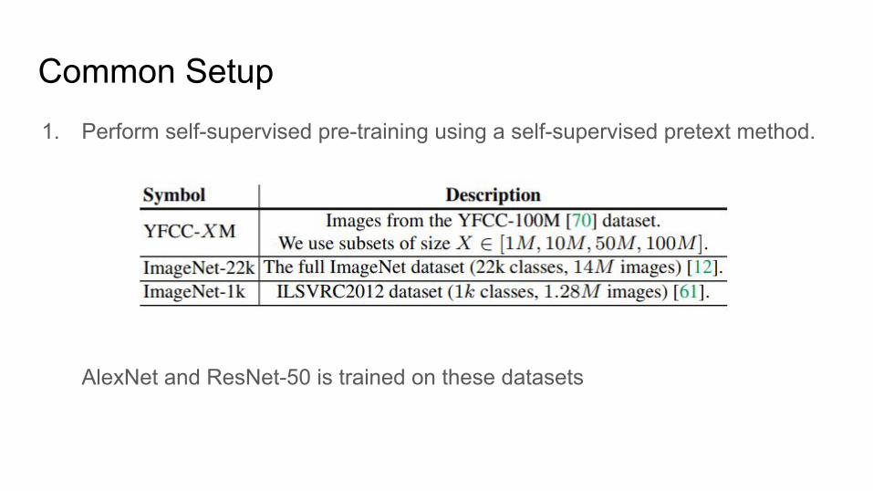
Task 1. Image Classification

● 3 datasets are used: Places205, VOC07 and COCO2014.

● Batch size = 256; learning rate of 0.01 decayed by a factor of 10 after every 40k iterations.

● Train for 140 iterations using SGD on the train split.

Task 1. Image Classification3 datasets are used: Places205, VOC07 and COCO2014.

ResNet-50 top-1 center crop accuracy for linear classification AlexNet top-1 center crop accuracy for linear classification

both the supervised pre-training and benchmark transfer tasks solve a semantic image classification problem.

Task 2. Low-shot Image Classification

What if the number of per-category examples are low?

● Vary the number k of positive examples per class

● Evaluate only for ResNet50

● Average and standard deviation of 5 independent examples

Task 2. Low-shot Image Classification

Best performing Layer res4 for Resnet-50 on VOC07 and Places-205

low-shot

high-shot

Task 3. Visual NavigationScenario:

● An agent receives a stream of images as input● navigate to a predefined location● Spawned at a random start point● How to build a map?

Setup:● Train a agent using reinforcement learning in the Gibson environment● Uses fixed feature representations from a ConvNet and only update the policy network● Separately train agents for layers res3, res4, res5 of a ResNet-50

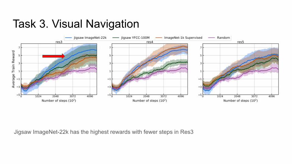
Jigsaw ImageNet-22k has the highest rewards with fewer steps in Res3

Task 3. Visual Navigation

Task 4. Object Detection Setup:

● Detectron framework to train the fast R-CNN object detection model.● Selective search on the VOC07 and VOC07-12 datasets● Freeze the full conv budy of Fast R-CNN and only train the Rol heads● Same training schedule for both supervised and self-supervised methods● Slightly longer schedule to improve object detection performance● 2 GPUs at 22k/8k(VOC07) and 66k/14k(VOC7_12)

Task 4. Object Detection

the self-supervised initialization is competitive with the ImageNet pre-trained initialization on VOC07 dataset even when fewer parameters are fine-tuned on the detection task.

Setup:

● Use NYUv2 dataset which contains indoor scenes and PSPNet architecture

● Fine-tuned res5 onwards and train with same hyperparameters.

● Batchsize of 16, learning rate of 0.02 decayed with a power of 0.9 and SGD for optimization

Task 5. Surface Normal Estimation

Task 5. Surface Normal Estimation

Metrics: the angular distance(error) of the prediction and the percentage of pixels within t degree of the ground truth

SummarySelf-supervised learned representation:

Outperforms supervised on surface normal estimation

` performs competitively base on navigation tasks

Match the supervised object detection baseline with limited fine-tuning

Performs worse on image classification and low-shot classification.