Success in mathematics for statistics - WikispacesrefreshSIMS.pdf · 1.2 Success in maths for...
178
Success in maths for statistics Learning and Teaching Support Unit (LTSU) The Learning Centre
-
Upload
truongthuan -
Category
Documents
-
view
226 -
download
4
Transcript of Success in mathematics for statistics - WikispacesrefreshSIMS.pdf · 1.2 Success in maths for...

Success in maths for statisticsLearning and Teaching Support Unit (LTSU)The Learning Centre

Published by
University of Southern QueenslandToowoomba Queensland 4350Australia
http://www.usq.edu.au
© University of Southern Queensland, 2007.2.
Copyrighted materials reproduced herein are used under the provisions of the Copyright Act 1968 as amended, or as a result of application to the copyright owner.
No part of this publication may be reproduced, stored in a retrieval system or transmitted in any form or by any means electronic, mechanical, photocopying, recording or otherwise without prior permission.
Produced by the Distance and e-Learning Centre using FrameMaker7.1 on a Pentium workstation.

Success in maths for statistics
Learning materials prepared by
Linda Galligan
Joan Mohr
Janet Taylor
From The Learning Centre
Ph: 07 4631 2751
Fax: 07 4631 1801
Email: [email protected]


Table of contents
Page
1 Arithmetic and the calculator
Aims 1.11.1 Our number system 1.11.2 Positioning numbers 1.2
1.2.1 Fractions 1.31.2.2 Absolute value 1.3
1.3 Rounding numbers 1.41.4 Working with numbers 1.6
1.4.1 Addition 1.61.4.2 Subtraction 1.91.4.3 Multiplication 1.111.4.4 Division 1.16
1.5 Order of calculation 1.191.6 Percentages 1.23
1.6.1 Converting from a fraction to a percentage 1.231.6.2 Converting from a percentage 1.28
Solutions 1.34
2 Formulas
Aims 2.12.1 Introduction 2.12.2 Simplifying expressions 2.22.3 Relationships in words 2.72.4 Relationships as formulas 2.72.5 Substituting into formulas 2.112.6 Rearranging formulas 2.15Solutions 2.23

3 Graphing
Aims 3.13.1 Describing a relationship from a graph 3.13.2 Relationships as graphs 3.6
3.2.1 The Cartesian plane 3.73.2.2 Drawing graphs 3.15
3.3 Gradients of line graphs 3.243.3.1 Finding the gradient of a given line 3.323.3.2 Drawing a line, given the gradient 3.35
3.4 Linear equations 3.39Solutions 3.46
4 Statistics
Aims 4.14.1 Introduction 4.14.2 Collecting data 4.24.3 Organising and displaying data from tables 4.54.4 Organising and displaying raw data 4.11
4.4.1 Frequency distribution table 4.114.5 Analysing data 4.14
4.5.1 Where is the centre of these data? 4.144.5.2 How much spread is in the data? 4.22
4.6 Data with two variables 4.24Solutions 4.31

Module 1 – Arithmetic and the calculator
Module 1
Arithmetic and the calculator1


Module 1 – Arithmetic and the calculator 1.1
Aims
Many students find Data Analysis a difficult subject. It requires learning difficult concepts but also an understanding of the underlying mathematics. This module aims to review some basic arithmetic calculations and look at how these are performed on the calculator.
On successful completion of this module you should be able to:
• give examples of different types of numbers;
• perform the operations of addition, subtraction, multiplication and division on all of the above numbers;
• perform complex calculations using order of operation;
• use techniques of estimation to aid in calculation;
• use percentages; and
• use a calculator for calculations.
1.1 Our number system
The numbers and symbols that we use in mathematics are a part of our language. If we have a common understanding of what numbers mean and say, we can be assured that the message we want to send will be received as it was intended. When we communicate with numbers, just as with words, we have to be aware of the purpose of the message as well as the audience with whom we are communicating.
The number system we use today has developed over many hundreds of years. Early civilisations only counted using fingers and toes where necessary. When it became necessary for additional representation of number, piles of stones were used. Eventually these needed to be grouped to make counting easier. Although we now group our numbers in lots of ten, early civilisations used other groupings for their number systems. For example some grouped in lots of five because they were used to seeing five fingers and five toes on each hand and foot. Another grouping that is still in use today is 60. The Babylonian civilisations used this for counting and we continue with its use for measurement of time (60 minutes in 1 hour, 60 seconds in 1 minute).
The system of numbers we use today is called the Hindu-Arabic system. It consists of the digits 0, 1, 2, 3, 4, 5, 6, 7, 8 and 9 believed to have been used by the Arabs before being adopted by other countries. This system differed greatly from other systems because of the inclusion of a symbol for zero. Our system of numbers is made up of many different types of numbers – whole numbers, negative numbers, fractions, decimals etc. and you need to know how to manipulate these types of numbers in statistics.

1.2 Success in maths for statistics
1.2 Positioning numbers
Let’s picture numbers on the number line. This allows us to see these numbers in order, moving from small to large. To draw a number line we draw a line and choose any point to represent zero (0). With a ruler we then mark off even spaces along the line to the right.
The arrows at the end of the line means that the numbers keep going, getting larger and larger (forever!!) or smaller and smaller. We call the imaginary point that we never reach at the end of this number line, infinity or negative infinity. It is given the symbol ∞ or –∞. Over history there has been much discussion about the concept of infinity. It is still a concept that is very hard to grasp. We do know that the first person to use the symbol ∞ for infinity was Englishman John Wallis in a publication in 1655.
Let’s look at some features of the number line.
You know that 3 is a number less than 5 and we can represent this as 3 < 5. The symbol ‘<’ means less than.
If you look at the number line above you will see that the number 3 is to the left of 5. This also indicates that 3 < 5.
The opposite symbol to less than is greater than represented by the symbol ‘>’.
An example of this would be to say that 4.8 > 4.2 or 4.8 is greater than 4.2. You can imagine that 4.8 is further along the number line than 4.2 and hence is greater than 4.2.
You should note that the ‘point’ of the < or > sign will always point to the smaller number while the ‘open side’ will always point to the larger number.
The following two symbols are an extension of the above:
≤ which means less than or equal to; and≥ which means greater than or equal to
For example 3, 7 and 9 are all less than or equal to 9, while 12, 17 and 98 are all greater than or equal to 12.
−3 −2 −1 0 1 2 3 4 5
∞
Module 1 – Arithmetic and the calculator 1.3
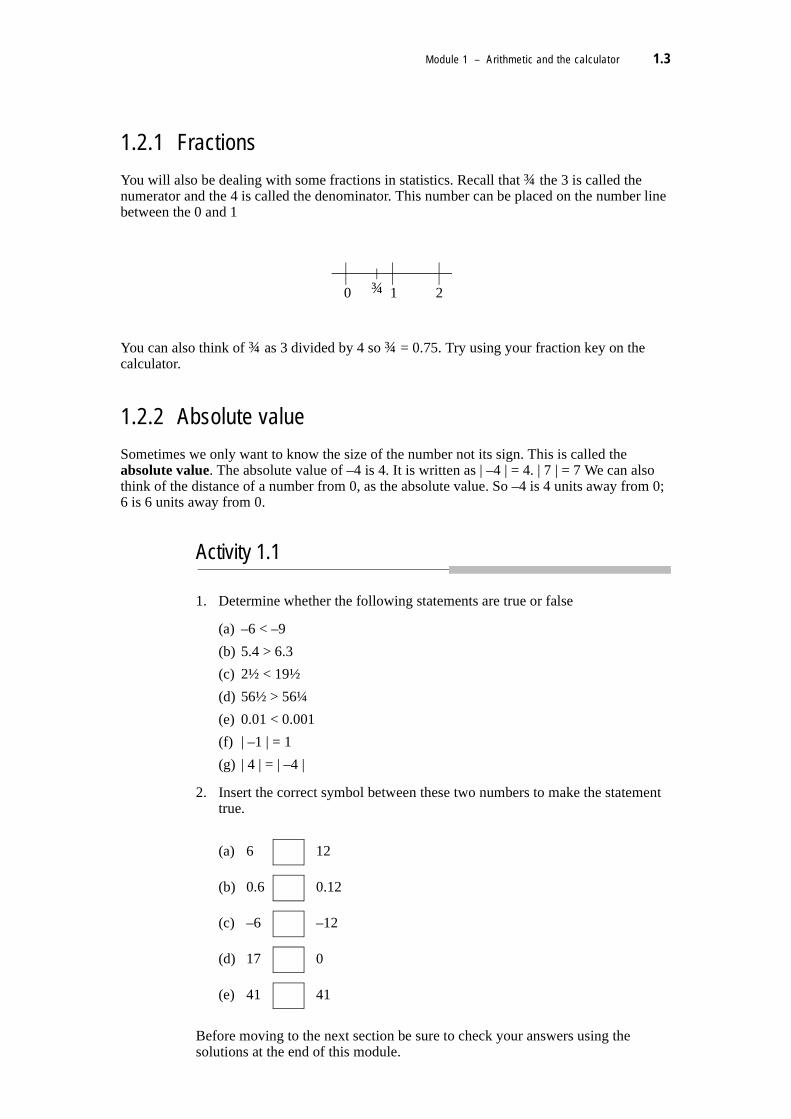
1.2.1 Fractions
You will also be dealing with some fractions in statistics. Recall that ¾ the 3 is called the numerator and the 4 is called the denominator. This number can be placed on the number line between the 0 and 1
You can also think of ¾ as 3 divided by 4 so ¾ = 0.75. Try using your fraction key on the calculator.
1.2.2 Absolute value
Sometimes we only want to know the size of the number not its sign. This is called the absolute value. The absolute value of –4 is 4. It is written as | –4 | = 4. | 7 | = 7 We can also think of the distance of a number from 0, as the absolute value. So –4 is 4 units away from 0; 6 is 6 units away from 0.
Activity 1.1
1. Determine whether the following statements are true or false
(a) –6 < –9(b) 5.4 > 6.3(c) 2½ < 19½(d) 56½ > 56¼(e) 0.01 < 0.001(f) | –1 | = 1(g) | 4 | = | –4 |
2. Insert the correct symbol between these two numbers to make the statement true.
Before moving to the next section be sure to check your answers using the solutions at the end of this module.
(a) 6 12
(b) 0.6 0.12
(c) –6 –12
(d) 17 0
(e) 41 41
0 1 2¾

1.4 Success in maths for statistics
1.3 Rounding numbers
When performing calculations, particularly on the calculator, you are going to get answers that have many decimal places. It is not normally necessary to report all of these places. You should round your answer.
It is important that you never round off before you get to the final answer.
You may be asked to round in a number of ways.
You could be asked to round a number to a specific place value or to a given number of decimal places. The following method is applied in both of these cases.
To round numbers to a particular place value, investigate the digit immediately to the right of it.
• If the digit immediately to the right is greater than or equal to 5 (i.e. ≥ 5, which includes the digits 5, 6, 7, 8 or 9), then increase the required place value by 1. We say the number has been rounded up.
• If the digit to the right is less than 5 (i.e. < 5 which includes the digits 0, 1, 2, 3 or 4), then the required place value remains the same. We say the number has been rounded down.
• All digits to the right of the round off place are replaced by zeros.
Let’s look at some examples:
Example
Round 572 to the nearest hundred.
The digit immediately to the right of the hundreds column is greater than or equal to 5 so the digit in the hundreds column is increased by 1. The 5 in the hundreds place will increase to 6
All place values to the right of the required position are then filled with zeros.
So 572 rounded to the nearest hundred becomes 600.
We could picture this on the number line.
hundreds position(the 5)
look at the digit immediately to the right(the 7)
572
500 550 600
We can see that 572 is closer to 600 than to 500.

Module 1 – Arithmetic and the calculator 1.5
Example
Round 674 927 to the nearest ten thousand.
The digit immediately to the right of the ten thousands column is less than 5 so the digit in the ten thousands column remains the same.
All place values to the right of the required position are then filled with zeros.
So 674 927 rounded to the nearest ten thousand becomes 670 000
Activity 1.2
Complete the following table by rounding each number as indicated.
When rounding decimal numbers we use much the same method as we used with whole numbers. The only difference is that when the round-off position is after the decimal point, we do not fill any spaces with zeros.
Example
Round 3.648 to the nearest tenth
As before, look at the digit to the right of the tenth position, in this case the 4. It is less than 5 so we leave the digit in the tenths position as it is.
3.648 ≈ 3.6 rounded to the nearest tenth.
The symbol ≈ means approximately equal to. So we would read the above statement as 379 is approximately equal to 400.
You may also see the symbols ≈ or ≅ used to represent ‘approximately equal to’ but in these modules we will continue to use ≈
Number To nearest thousand
To nearest hundred
To nearest ten
(a) 2 575
(b) 324
(c) 105
(d) 26 897
(e) 5 502 471
ten thousands column(the 7)
look at the digit immediately to the right(the 4)
674 927

1.6 Success in maths for statistics
Example
Round 3 476.638 to two decimal places.
To end up with two decimal places we are rounding to the nearest hundredth. Look at the digit to the right of the hundredth place, in this case the 8. It is greater than or equal to 5 so we take the round-off place up by one.
3 476.638 ≈ 3 476.64 rounded to two decimal places.
Activity 1.3
1. Round these numbers to the place value indicated.
In any calculations that follow it is always good practice to quickly estimate the answer before you calculate. Having done this you can be sure that your answer is ‘close to the mark’. We would expect you to follow this practice throughout the rest of these modules wherever possible.
1.4 Working with numbers
You will probably remember all or parts of the following from your previous studies. Although everybody should work through all sections, some people may move more quickly than others. If you are unsure, take your time, this groundwork is very important.
In mathematics there are four basic operations to perform: addition, subtraction, multiplication and division. We will deal with each of these in turn.
1.4.1 Addition
Example
On a recent weekend trip I travelled the following distances each day.
(a) 576.205 to the nearest hundredth
(b) 75 201.3 to the nearest unit
(c) –0.008 to the nearest hundredth
(d) 67.345 67 to one decimal place
(e) –6 399.998 to two decimal places
Friday Saturday Sunday Monday356.3 km 126.9 km 91.1 km 402 km

Module 1 – Arithmetic and the calculator 1.7
To find the total distance travelled on this weekend trip I need to find the sum of the distances for each day. That is, I must add together each of the above distances.
Before doing any calculation we should estimate the answer. It is easy on the calculator to press the wrong key and end up with an incorrect answer. If we estimate the answer first, we should then be aware that our answer may be wrong, if the estimated and calculated answers differ by a large amount.
The most convenient way to estimate is to round each number to its leading digit.
The total distance travelled then would be approximately equal to
400 + 100 + 90 + 400 = 990 km
Example
The following showed the profit of my son’s ‘business’ over 4 weeks:
What was his total profit for the month?
To answer this we must add 6, –3, 5, and –7.
To do this you must find the +/– key or the (–) key on your calculator.
His profit for the 4 weeks was $1!
Find how to add numbers on your calculator, including how to use:
• the cancel keys
• fraction keys
• the negative key
Activity 1.4
Find the following answers without using a calculator. Estimate your answer before commencing. Check your answer by using a calculator.
356.3 ≈ 400126.9 ≈ 100
91.1 ≈ 90402 ≈ 400
$6 $–3 $5 $–7
1. (a) 58 + 61
(b) 25.01 + 956.5+ 0.32
(c) 0.750 + 0.023 05 +0.10 + 0.9 + 0.003 15
(d) 658 + 0

1.8 Success in maths for statistics
2. The children’s ward of the local hospital admitted 5 children on Sunday, 3 on Monday, 2 on Tuesday, none on Wednesday and Thursday but 6 on Friday and 9 on Saturday. How many children were admitted to the children’s ward for the week?
3. The attendances for the Bold Batters Baseball Club’s first four home games were 10 428, 8 922, 7 431 and 9 647. How many people came to the first four home games?
4. David’s lunch consisted of a triple hamburger that contained 2 103 kJ (kilojoules, the measure of energy in food), hot potato chips containing 1 714 kJ, an apple pie with 1 148 kJ and a diet soft drink containing just 18 kJ. How many kilojoules did David consume for lunch?
5.
6. Complete these without a calculator and then check your answers with the calculator.
(a) –5 + 3
(b) –5.6 + 78
(c) 0.456 + –67
(d) 89 + –567
(e) –1.789 + 1.674
7. Translate each of the following questions into an expression involving a sum and then solve. A diagram may sometimes help you to estimate whether the answer will be positive or negative.
(a) Naomi owes $25. If she is able to pay back $5, how much does she still owe?
(b) A submarine dived 37 metres and then rose 23 metres. What is its new depth?
(c) Australia started their second innings in the cricket, 134 runs behind South Africa’s first innings total.
(i) If the opening partnership scored 76 runs, what is Australia’s position?
(ii) If Australia scored 475 runs in their second innings, what is their position at the end of the innings?
(d) From a certain floor in a building the lift descended 3 floors. It then rose 6 floors before descending 8 floors. What is the lift’s final position relative to its starting position?
1 3(a) 5 4
3 1(b) 3 14 2
+
+

Module 1 – Arithmetic and the calculator 1.9
1.4.2 Subtraction
Example
On my previously mentioned weekend escape, I took $300. My expenses for the weekend totalled $121.
To find the amount of money I came home with I must subtract these expenses from the original amount of money. We call this the difference between the amount of money I took with me and the expenses.
That is, $300 – $121
Firstly, estimate the remaining amount.
300 = 300121 ≈ 100
300 – 100 = 200 The remaining money is about $200
We can now do this subtraction on the calculator.
Find the – key on your calculator.
Key in 300 – 121. The display should read 179
$179 is close to our estimate of $200 so is a reasonable answer. The amount of money I had left after the weekend escape was $179.
Example
One concept that you will use in statistics is the difference between the average of a set of scores and a particular score. Look at the following examples and pay particular attention to the negative sign. We will look at these examples in a later module on formula.
The average take home pay for a group of people was $872. If you earned $697, how far from the average were you?
697 – 872 = –175
So you were $175 below the average.
The average temperature in December in a Northern Hemisphere country is –10° C. If the temperature one December day was 5°. How far from the average was this temperature?
5 – –10 = 5 + 10 = 15
So the temperature was 15° above normal. Note here subtracting a negative is the same as adding.

1.10 Success in maths for statistics
Activity 1.5
Find the following answers without using a calculator. Estimate your answers before you commence. Check your answers with a calculator.
2. The average profit for a company over the last 4 years was $–5 000. If this year’s profit was $8 000, how far from the average was this years profit?
3. A cleaner is asked to dilute 542 mL of disinfectant concentrate by making it into 3 500 mL of diluted solution. How much distilled water will they need to add? A diagram may help you ‘picture’ this situation.
4. The following table shows the weekly pay schedule for a number of employees of a small company. Gross pay is the amount of money you receive before any deductions. Deductions for these employees include taxation, superannuation and union fees. After these deductions have been made, the amount remaining is the take home pay.
(a) For each employee calculate the take home pay.
(b) What is the total wages bill for these employees (Gross Pay)?
(c) What amount of money will be sent to the taxation office on behalf of these employees?
5.
1. (a) 759 – 326
(b) 39.2 – 14.125
(c) 1.264 30 – 247.2
(d) 3.7 – 0
(e) 7 – –2
Name Gross Pay Tax Superannuation Union
FeesTake
Home Pay
Adams J $500 $105 $30 $2Bull P $1 200 $407 $74 $2Filbee Y $678 $169 $41 $2Hand I $893 $261 $54 $2Ruse K $560 $127 $34 $2Totals
6 1(a) 2 57 122 1(b)
123 23
−
−

Module 1 – Arithmetic and the calculator 1.11
Statistics deals a lot with uncertainty. We often talk about a range of values instead of an exact amount. For example the profit for next year will be one million dollars plus or minus a few hundred thousand. We can express symbolically as:
$1 000 000 ± $200 000
This means the profit could be as high as $1 200 000 or as low as $800 000.
Activity 1.6
1. Interpret the following:
(a) 7.34 ± 0.06
(b) 0 ± 15
(c) $21 000 ± $1 000
1.4.3 Multiplication
Example
Suppose a builder is prepared to employ you as a casual labourer for $80 a day.
Your total weekly pay would be: $80 + $80 + $80 + $80 + $80 = $400
This is the same as saying 5 lots of $80 added together.
A short hand way to write 5 lots of $80 added together is to use multiplication.
That is, 5 × 80 = 400
We say five multiplied by eighty equals four hundred.
We call 5 and 80 factors of 400 and say that 400 is the product of 5 and 80.
You may be familiar with these terms in everyday language. For example, ‘one of the factors leading to an early arrest was the accurate description given to police by the witness’. This simply means a part of the reason for the early arrest was the good description. We could also say ‘the reason for an early arrest was a product of good police work and an observant witness’. We are saying that the early arrest was a combination of these two factors.
Multiplying numbers on the calculator
Find the × key on your calculator
Multiply 5 by 80
The display should read 400

1.12 Success in maths for statistics
The multiplication of decimals and fractions less than one is a bit more difficult to understand. For example when multiplying one half by a half the answer is a quarter. If you had half a cup of water and someone wanted half of it, they would get a quarter of a cup, i.e.:
Or we could say 0.5 × 0.5 = 0.25. Remember when you are multiplying by fractions or decimals between 0 and 1 your answer is going to be less than your original numbers.
To multiply numbers involving negatives remember:
• Positive multiplied by Negative is negative, e.g. 7 × –4 = –28• Negative multiplied by Negative is positive, e.g. –7 × –4 = 28
Activity 1.7
Find the following answers without using a calculator. Estimate your answers before you commence. Check your answer with a calculator.
2. Sally earns $14.80 per hour and works for 38 hours in a week. How much does Sally earn?
3. Your blood alcohol concentration (BAC) is measured in grams of alcohol per 100 mL of blood. If 50 mL of blood was drawn from a driver and 0.02 grams of alcohol was measured, what would the BAC of the driver be?
4. Jeremy sees a shirt normally priced at $45 on sale for only $26.
(a) How much would Jeremy save if he purchased a shirt at the sale price?
(b) Jeremy decides to buy 5 shirts in different colours. How much does he save by buying them all at the sale price?
5. An express coach from Brisbane to Melbourne stops to load and unload passengers only in Sydney.
1. (a) 9 × 45
(b) 0.9 × 7
(c) 1.95 × 0.2
(d) 2 000 × 346
(e) 4.2 × 0.38
(f) –500 × 4 000
(g) –52 × –21
Number of passengers
City Loaded Unloaded
Brisbane 36Sydney 23 14
Melbourne

Module 1 – Arithmetic and the calculator 1.13
(a) How many passengers travelled all the way from Brisbane to Melbourne?
(b) How many passengers got off the coach in Melbourne?
6. The average winter temperature in a city if –5oC. Another city is twice as cold. What is the average winter temperature in this city?
7. Calculate the following:
(a)
(b) 0.24 ×
(c) 0.4 × 0.37
(d) 4.2 × 0.5
Power notation
Often you will see different symbols being used as ways to reduce the writing out of a long process. So far we have used multiplication as a short hand way of writing repeated additions. Power notation is a shorthand way of representing the same numbers being multiplied together several times.
Consider 6 × 6. This could be written 62. We would say six squared or six to the power two.
62 indicates that we are multiplying together two numbers which are both 6.
6 × 6 × 6 then would be written 63 and would mean that we are multiplying three numbers together which are all 6. We say six to the power three or six cubed.
See if you can write out and describe in words what is meant by 65
..................................................................................................................
Did you say something like 65 means 5 numbers which are all 6 are multiplied together to give 6 × 6 × 6 × 6 × 6 ?
What if the numbers are negative? –6 × –6 = 36 so (–6)2 = 36.
Any number squared will be positive.
To evaluate powers on the calculator
There are two buttons on your calculator that we can use to evaluate powers
Find the x2 key
and the xy key
The x2 key is only for finding powers of 2.
Evaluate 62
2 17 3
×
110
1.14 Success in maths for statistics
The display should read 36.
This key is very useful when finding powers of two but the key for finding all powers including 2 is the xy key.
Evaluate 53
The display should read 125
You may not have had to use these two new keys before so here is an activity if you feel you would like more practice.
Activity 1.8
1. Evaluate the following without a calculator. Check your answers with your calculator.
(a) 33
(b) 24
(c) (–5)4
(d) 41
(e) 0.94
(f) 0.065
2. Complete:
(a) 4 = 16 (How many times is 4 multiplied together to give 16?)
(b) 2 = 32
(c) 5 = 25
(d) 3 = 81
3. The Heptane family has seven children. Each of the seven children spends 7 minutes per day reading. What is the total time the children spend on reading in one week?
4. In statistics you will find a number called the variance. It is the square of another important concept in statistics called the standard deviation. If the standard deviation is 0.7, what is the variance?
The square root
What if a question on powers asked you to find a positive number that when raised to the power 2 gave you 49 as the answer.
That is 2 = 49
Did you get 7 for this answer?

Module 1 – Arithmetic and the calculator 1.15
We have a shorthand way to express this type of question.
We could write √49 and it is understood that we are meant to find the two identical numbers that multiply to give 49.
We would read √49 as the square root of 49
The symbol we use for the square root is √
To evaluate square roots on the calculator
Find the √ key on your calculator
Evaluate √49.
The display should read 7
Find the square root of 0.25
√0.25 = 0.5
Notice the square root of a number between 0 and 1 gives a larger answer. This is because 0.5 × 0.5 = 0.25 (recall page 11).
If we multiply 7 × 7, we get 49. But if we multiply –7 × –7 we also get 49. So we can say √49 = 7 or –7. This is sometimes written as ±7 (read this as plus or minus 7). Notice your calculator will only give you the positive answer. You will have to decide for yourself if you need to consider the negative answer.
Activity 1.9
1. Find a positive answer for the following. Check your answers on the calculator.
(a) √81 Remember, we are asking what two identical numbers multiply to give 81.
(b) √36
(c) √25
(d) √64
(e) √100
(f) √0.81
2. Evaluate the following on your calculator – give two possible answers.
(a) √4.2
(b) √0.05
(c)
3. In statistics the standard deviation of a number is the square root of the variance. If the variance is 8.4, what is the standard deviation?
25.3 2.7+

1.16 Success in maths for statistics
1.4.4 Division
Recall that multiplication is a shorthand way of adding the same number many times. Similarly, division is a shorthand way of subtracting the same number several times.
For example, to determine how many 5’s are contained in the number 20, you could use subtraction as follows:
Using subtraction it has taken four steps to determine how many 5’s there are in 20. A shorthand way of writing this using division would be
We would say this as twenty divided by five equals four.
We call the result of division a quotient. In our example above the quotient is 4.
It is interesting to note that the word quotient comes from the Latin word quotiens meaning ‘how often’ or ‘how many times’.
Dividing by a negative or into a negative number gives a negative. For example
–21 ÷ 3 = –721 ÷ –3 = –7
Dividing Numbers on the Calculator
Find the ÷ key on your calculator.
Divide 20 by 5
The display should read 4
We can say that 20 ÷ 5 = 4 because there are 4 lots of 5 in 20
i.e. 4 × 5 = 20
Can you see that division is the opposite of multiplication. Knowing your multiplication tables will be a help when doing division as well as multiplication.
For example:
Before we move on to the next section let’s consider divisions involving zero and divisions involving decimals and fractions.
20 – 5 = 15 one step15 – 5 = 10 two steps10 – 5 = 5 three steps 5 – 5 = 0 four steps
20 ÷ 5 = 4
72 ÷ 8 = 9 since 9 × 8 = 7245 ÷ 9 = 5 since 5 × 9 = 45

Module 1 – Arithmetic and the calculator 1.17
Zero
What happens when it is zero that we are dividing by?
For example, 7 ÷ 0 = ? since ? × 0 = 7
We know that anything multiplied by zero equals zero so there is no number that we can write instead of the ? sign.
We say that division by zero is undefined. That is, it is impossible to divide by zero.
Try 7 ÷ 0 on your calculator. You should get an error message (– E –)
Decimals & fractions
When dividing by numbers between 0 and 1, our answers are going to be larger than our original. Look at the following examples:
There is 21mL of medicine to be put into ampoules that will contain only 0.2mL. How many ampoules should there be?
21 ÷ 0.2 = 105
So we need 105 ampoules.
Example
In a kindergarten, there are 25 children and each child has an apple. Apples have been divided into quarters. How many quarters are there?
25 ÷ = 100
So there are 100 quarters.
0 ÷ 6 = 0 since 0 × 6 = 0 No cake divided among 6 children!0 ÷ 342 = 0 since 0 × 342 = 0
14

1.18 Success in maths for statistics
Activity 1.10
1. Complete the following without using a calculator. Estimate your answer before you begin. Check your answer with the calculator.
(a) 1 204 ÷ 4
(b) 432 ÷ 12
(c) 10 608 ÷ 26
(d) 3612 ÷ 42
2. Three children were left a $4 500 inheritance. How much will each child receive?
3. Joseph purchased 2 700 grams of minced steak to be used for 6 family meals. He wishes to freeze the meat in meal size portions. What amount of mince should he use for each meal?
4. If you receive and annual salary of $31 025, what is your weekly wage? Hint: you will need to work out the daily rate (365 days in a year) and then the weekly rate.
5. A merry-go-round at the local show revolves once every 32 seconds. Keely’s ride lasts 8 minutes, how many times did the merry-go-round revolve? (Hint: 8 minutes equals 8 × 60 = 480 seconds)
6. Calculate the following:
(a) 2.8 ÷0.4
(b) 2 600 ÷ –0.07
(c) 23 ÷ 29

Module 1 – Arithmetic and the calculator 1.19
1.5 Order of calculation
So far we have been dealing with expressions involving just one operation, for example
–12 × 6 =
However, in reality, calculations usually involve performing more than one operation.
Consider the following situation. We are asked to calculate the amount earned by a person working for 12 hours if the pay rate is $14 per hour for the first 8 hours and $17 for each hour after that.
This means that the person is working 8 hours at $14 per hour and 4 hours at $17 per hour. We can express this mathematically as
8 × $14 + 4 × $17
Look carefully at this expression. Note that there are three operations: a multiplication, an addition and another multiplication.
The order in which the operations are performed will determine our final result. Two possibilities are presented below.
Obviously only one answer can be right! Unfortunately for the person involved, Possibility 2 is the correct answer and the amount earned is $180 for the 12 hours work.
Mathematical expressions are written to convey specific information, therefore everyone reading them needs to interpret them the same way. For this reason, mathematicians have established a convention (an accepted method) that specifies the order in which operations are to be performed.
Possibility 1
8 × $14 + 4 × $17= $112 + 4 × $17 Evaluate Multiplication= $116 × $17 Evaluate Addition= $1 972 Evaluate Multiplication
Possibility 2
8 × $14 + 4 × $17= $112 + 4 × $17 Evaluate Multiplication= $112 × $68 Evaluate Multiplication= $180 Evaluate Addition

1.20 Success in maths for statistics
This order of operations convention can be stated as:
When working from left to right
* If there are brackets inside another set of brackets, do the inside brackets first.
If you check Possibility 2 above, you will see that it follows the convention for the order of operations, whereas Possibility 1 does not.
This is a very important aspect of mathematics that you must ensure that you understand.
Follow through the examples below carefully.
Example
Evaluate 12 + 2 × 3
Let’s check this answer on the calculator. If you have a scientific calculator it will automatically apply the order of operation convention.
On your calculator press 1 2 + 2 × 3 = The display should read 18
Example
Evaluate 8 – 12 ÷ (7 – 4)
To check this on the calculator you will need to find the keys for brackets on your calculator. Notice that there are opening brackets as well as closing brackets.
Step 1 Evaluate any expressions in brackets* first.Step 2 Evaluate any powers and rootsStep 3 Evaluate any multiplications or divisions Step 4 Evaluate any additions or subtractions
12 + 2 × 3 Evaluate the multiplication first= 12 + 6 Finally evaluate the addition= 18
8 – 12 ÷ (7 – 4) Evaluate the brackets first= 8 – 12 ÷ 3 Next do the division= 8 – 4 Finally the subtraction= 4
Module 1 – Arithmetic and the calculator 1.21
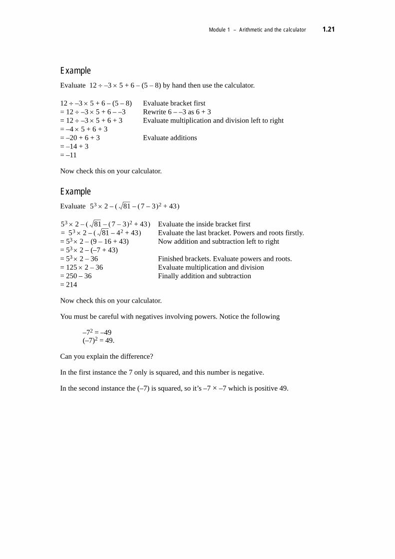
Example
Evaluate 12 ÷ –3 × 5 + 6 – (5 – 8) by hand then use the calculator.
Now check this on your calculator.
Example
Evaluate
Now check this on your calculator.
You must be careful with negatives involving powers. Notice the following
–72 = –49 (–7)2 = 49.
Can you explain the difference?
In the first instance the 7 only is squared, and this number is negative.
In the second instance the (–7) is squared, so it’s –7 × –7 which is positive 49.
12 ÷ –3 × 5 + 6 – (5 – 8) Evaluate bracket first= 12 ÷ –3 × 5 + 6 – –3 Rewrite 6 – –3 as 6 + 3= 12 ÷ –3 × 5 + 6 + 3 Evaluate multiplication and division left to right= –4 × 5 + 6 + 3= –20 + 6 + 3 Evaluate additions= –14 + 3= –11
Evaluate the inside bracket firstEvaluate the last bracket. Powers and roots firstly.
= 53 × 2 – (9 – 16 + 43) Now addition and subtraction left to right= 53 × 2 – (–7 + 43)= 53 × 2 – 36 Finished brackets. Evaluate powers and roots.= 125 × 2 – 36 Evaluate multiplication and division= 250 – 36 Finally addition and subtraction= 214
53 2 81 7 3–( )2– 43+( )–×
53 2 81 7 3–( )2– 43+( )–×53 2 81 42– 43+( )–×=

1.22 Success in maths for statistics
Activity 1.11
1. Evaluate the following without a calculator. Check your results on the calculator.
2. Evaluate the following without a calculator. Estimate your answer before calculating. Check your results on the calculator.
(a) 765 ÷ 15 + 822
(b) 89 + 21 – 48 × 23
(c) 591 + 372 × √49
(d) 4 763 + 395 ÷ 5 × 16
(e) (62 – 242 + (7 + 3 × 81) – √169) + 61 × 453
3. At Andy’s Engineering Works the hourly rate for workers is $14. Overtime is paid at $21 per hour, while working on a public holiday pays $28 per hour.
(a) Ahmid works as a spray painter. In one busy week Ahmid worked 32 normal hours and 8 hours on Monday which was a public holiday. How much money did Ahmid earn in this week.
(b) Mary works as an electrician. To catch up on outstanding work Mary agreed to work 8 hours on Show Day, a public holiday. She worked the other four days of the week at 8 hours of normal time and 2 hours of overtime each day. How much money did Mary earn in this week.
4. A coach can carry a maximum of 43 passengers. If the average passenger weighs 54 kg and carries luggage weighing 12 kg what is the usual ‘load’ for the full coach carries.
5. An express coach from Brisbane to Melbourne stops to load and unload passengers only in Sydney. What was the total amount paid by people using this coach?
(a) 7 × 5 + 4 (f) –3 ÷ –1 + 92 × –2
(b) 10 – 6 × 7 (g) 27 – √9 + 21 ÷ –3
(c) 6 + (3 – 9) (h) 4 × (2 + 5) ÷ (3 + 1)
(d) –2 – 2 × –3 (i) (17 – 53) ÷ –3 + 9 × –5
(e) 9 ÷ 3 × 7 + 3 (j) (–5 × –4)2 – 6 ÷ (–3 + √4)
Single Fares:Brisbane – Melbourne $120Brisbane – Sydney $75Sydney – Melbourne $68
Number of Passengers
City Loaded Unloaded
Brisbane 36Sydney 23 14
Melbourne

Module 1 – Arithmetic and the calculator 1.23
1.6 Percentages
Percentages were first used in the fifteenth century for calculating interest, profits and losses. Currently they have a much broader application as indicated in the newspaper items below.
1.6.1 Converting from a fraction to a percentage
Let’s consider a person with the following marks over their first three assignments for a particular subject.
Because the assignments are all out of different marks, it is very hard just looking at these figures to decide which assignment has given the student the best result. A very convenient method of comparing these results is to make them all out of the same mark....100.
It is now quite easy to compare results and see that the first assignment gave the student the best result. We call the resulting comparison with 100 a percentage (from per cent meaning out of one hundred). We represent a percentage by the symbol %.
The percentage sign is thought to have been derived as an economy measure when recording in the old counting houses; writing in the fraction 25/100 of a cargo would take two lines of parchment, and hence the 100 denominator was put alongside the 25 and rearranged to become %.
Back to the above student’s assignment marks expressed as percentages:
Assignment 1 Assignment 2 Assignment 3 17/20 8/10 21/25
Assignment 1 85% Say 85 percent, meaning 85 out of 100.Assignment 2 80%Assignment 3 84%
...maths scores of the children who hadlearnt to play the piano leapt by 34 %
When you insure with NRMA youreceive a 10% discount on each policy
6% p aTerm Deposit
Surfboards, bodyboards and surfskiscaused 61% of injuries....
Clearance10 to 50% off everything.
Assignment 1 1720------ 17 5×
20 5×--------------- 85
100---------= =
Assignment 2 810------ 8 10×
10 10×------------------ 80
100---------= =
Assignment 3 2125------ 21 4×
25 4×--------------- 84
100---------= =

1.24 Success in maths for statistics
Rather than writing the assignment mark as a mark out of 100 we can simply multiply the fraction by 100 to get the value of the percentage.
Note that we are not changing the value of the fraction, just the look of it:
L
We can generalise this process.
When converting to a percentage, form a fraction and multiply by 100%.
Example
Consider the fictional property Gunadoo, a farm grazing cattle and sheep. In 1991 stock numbers indicated that times were good and food plentiful. By 1994 drought had taken its toll and Gunadoo had reduced its heard numbers. As things picked up after the drought Gunadoo again built up stock numbers. Below are the stock numbers for Gunadoo.
In which year did the farm have the greatest percentage of cattle compared to the entire stock?
We must firstly form a fraction and then multiply by 100% for each year.
17/20 = 85/100 = 85% the percent sign meaning out of 100.
1991 1994 1997Cattle 500 100 300Sheep 2 000 500 900
Assignment 1 1720------ 100%× 17 100%×
20 1×-------------------------- 85%= =
Assignment 2 810------ 100%× 8 100%×
10 1×----------------------- 80%= =
Assignment 3 2125------ 100%× 21 100%×
25 1×-------------------------- 84%= =
Percentage of cattle in 1991 Number of cattleTotal number of stock----------------------------------------------------- 100%×=
5002 000------------- 100%×=
500 100%×2 500
-----------------------------=
20%=

Module 1 – Arithmetic and the calculator 1.25
We can see from these figures that in 1997 Gunnadoo had the highest percentage of cattle.
Example
You pour out 200 mL from a bottle containing 1 000 mL. What percentage of the liquid did you pour out?
To do this on your calculator you would press the following keys.
2 0 0 ÷ 1 0 0 0 × 1 0 0 =
The display should of course read 20 and you will know to add the % sign.
As you can see it is often easier and quicker to do the calculation by hand using the technique of cancelling zeros.
Example
A team won 7 matches out of 8. What percentage did they win?
Percentage won = × 100% = 87.5%
(Check this on your calculator)
Percentage of cattle in 1994 Number of cattleTotal number of stock----------------------------------------------------- 100%×=
100600--------- 100%×=
100 100%×600
-----------------------------=
17%≈
Percentage of cattle in 1997 Number of cattleTotal number of stock----------------------------------------------------- 100%×=
3001 200------------- 100%×=
300 100%×1 200
-----------------------------=
25%=
Percentage poured amount poured outtotal amount
---------------------------------------------=
200 mL1 000 mL----------------------- 100%×=
200 mL 100%×1 000 mL
----------------------------------------=
20%=
78---

1.26 Success in maths for statistics
Example
Suppose I had painted 75 cm of a 3 m post. What percentage of the post has been painted.
As with previous examples, we cannot compare these two numbers while they are in differing units.
(Check this on your calculator)
Activity 1.12
1. Write as a percentage.
(a) 8 out of 10(b) 250 mL out of 400 mL(c) 800 g out of 2 000 g(d) 25 cm out of 80 cm(e) $25 out of $60(f) 50 mL out of 2 L(g) 2 × 10⁴ light years out of 3.5 × 10³ light years
2. In a class of 50 students taking a maths test, 45 passed. What percentage of the class passed?
3. In her life a green turtle lays an average of 1 800 eggs. Of these, some 1 395 don’t hatch, 374 hatchlings quickly die, and of the remaining 31, only 3 live long enough to breed. What percentage of the green turtle’s eggs hatch and live long enough to breed?
4. A survey of 200 people asking what cereal they ate for breakfast found the following results:
Cereal Number of people Percentage of peopleCorn Flakes 50
Rice Bubbles 42Nutri Grain 39Rolled Oats 23
Muesli 11Coco Pops 10
Other Cereals 25
Percentage painted 75 cm3 m
--------------- 100%×=
75 cm300 cm------------------ 100%×=
75 cm 100%×300 cm
-----------------------------------=
25%=

Module 1 – Arithmetic and the calculator 1.27
Complete the table by calculating the percentage of people eating each type of cereal.
5. Consider the following figures for pedestrians killed in Queensland in 1996.
(a) What percentage of all people involved in pedestrian accidents are killed?
(b) What percentage of the people involved in alcohol related accidents are taken to hospital?
(c) As a pedestrian, what is the most common way to be killed? What percentage of the total deaths, die in this way?
(d) We learn as a child that we should walk on the right hand side of the road so we are facing the approaching traffic. Do these figures still support this view? What figures did you compare to come to this decision?
What happens if we have a decimal that we wish to convert to a percentage? Since we can convert any fraction to a decimal equivalent, converting a decimal to a percentage is exactly the same process as converting a fraction to a percentage.
Example
Suppose that of the children under 6 believe in Santa Claus
× 100% = 75%
We are saying that 75% of the children under 6 believe in Santa Claus.
Now we know that = 3 ÷ 4 = 0.75
and that 0.75 × 100% = 75%
So, = 0.75 = 75%
So we can say that or 0.75 or 75% of the children under 6 believe in Santa Claus.
ALL AGES OVER 70 ALCOHOL LINKEDKilled – 55 Killed – 14 Killed – 16Taken to hospital – 405 Taken to hospital – 46 Taken to hospital – 65Treated at the scene – 381 Treated at the scene – 20 Treated at the scene – 43Minor Injuries – 153 Minor Injuries – 12 Minor Injuries – 11Total – 994 Total – 92 Total – 135
HOW PEDESTRIANS ARE KILLEDCrossing carriageway at traffic lights – 6
Crossing carriageway at pedestrian crossing – 1Crossing carriageway with no pedestrian control – 30
Stationary on road side – 6Walking against the traffic – 2
Walking with the traffic – 7Playing on the roads – 1
Other – 2
34---
34---
34---
Recall that multiplying by 100 moves the decimal point 2 places to the right.
34---
34---

1.28 Success in maths for statistics
Example
Convert 0.93 to a percentage.
Example
Convert 4.23 to a percentage.
1.6.2 Converting from a percentage
Example
A well known department store is offering 15% off everything in the shop on one particular day. You are very interested in a new clock which is normally selling for $35. What will the clock cost after the 15% discount?
Recall from a previous section that 15% means 15 per 100. As a fraction we can represent this
as
We could simplify this to be
We could also represent as a decimal.
15% = 15/100 = 0.15
You can work with a fraction or a decimal whichever you find most convenient.
Let’s return to our question. We must firstly calculate how much we would save.
Discount offered is 15% of $35
We can write this as 15% × $35 We write the ‘of’ as a multiplication sign.
= × $35
= × $35
= $5.25
0.93 0.93 100%×=93%=
4.23 4.23 100%×=423%=
15100---------
320------
15100---------
15100---------
320------

Module 1 – Arithmetic and the calculator 1.29
We could use decimals in the same way.
15% × $35
= × $35
= 0.15 × $35= $5.25
Either way we have a discount of $5.25.
The price you will pay for the clock on ‘discount day’ is $35 – $5.25 = $29.75
Example
Convert 75% to a fraction and a decimal.
Example
Convert 345% to a fraction and a decimal.
Did you notice that we ended up with a number greater than 1. This is because the percentage was greater than 100%.
Converting from a percentage to a fraction or decimal is a very useful skill. There are some percentages that we use so often that it is helpful to remember their fractional equivalents. This will also help in estimating answers which you should always be doing, even if only in your head.
Some of the common percentages are:
10% =
25% =
50% =
75% =
15100---------
75% 75100--------- 3
4---= =
0.75=
345% 345100--------- 69
20------= =
3.45=
110------
14---
12---
34---

1.30 Success in maths for statistics
Example
Convert 25½% to a fraction and a decimal
You know that 25% = = 0.25 so you would expect this answer to be very close to this result.
Depending on the circumstances, you might do this example in two different ways.
Depending on the circumstances, you might do the question like this:
This method is convenient if you are going on to do a calculation with your calculator.
Or, if calculating by hand you might do it like this:
Both of these answers are close to our estimate of or 0.25.
Let’s now look at some more practical uses for percentages.
Example
Interest is paid by a bank at a rate of 4% p.a. (Note: p.a. means per annum which is really saying per year). If you invested $2 000 for 2 years, how much money would you have?
Interest for two years = $80 × 2 = $160
At the end of the two years you would have $2 000 + $160 = $2 160
25½%=
Recall that dividing by 100 moves the decimal point 2 places to the left.
= 0.255
25½%=
To remove the decimal point, multiply top and bottom by 10.
Interest received for one year = 4% of $2 000 You could think here that 10% would give $200 a year and 5% is half of this at $100, so 4% must be a bit less than $100.
= × $2 000
= 0.04 × $2 000= $80
14---
25.5100----------
25.5100----------
25.5 10×100 10×----------------------=
2551 000-------------=
51200---------
14---
4100---------

Module 1 – Arithmetic and the calculator 1.31
Example
A hospital keeps on hand a 5% glucose solution (that is, a solution that is only 5% glucose). If the glucose container holds 500 mL what portion of the container is glucose?
5% of the container is actually glucose.
That is, 5% of 500 mL
So in a 500 mL container of 5% glucose solution, 25 mL would be glucose.
Example
In a recent survey of adult students returning to studying mathematics it was found that 49% of these students expressed some anxiety about this return to mathematics study. If the group consisted of 63 students how many were expressing some anxiety?
Let’s think about our answer before continuing. 49% is about 50% which we know is 1/2. If half the students are expressing anxiety this is about 31 or 32 students.
Now to the actual calculation.
We are to find 49% of 63
So approximately 31 of the 63 students expressed some degree of anxiety.
49% × 63
We can’t have a part of a student so we will round up.= 0.49 × 63= 30.87≈ 31
5100--------- 500 mL×=
5 500 mL×100
----------------------------=
25 mL=

1.32 Success in maths for statistics
Example
Let’s look again at Gunnadoo (from page 24). When the drought began to have an effect and stock numbers were reduced, what percentage of the cattle and sheep were removed?
Whenever we are looking at a percentage reduction or a percentage increase we must put the amount of the increase or decrease over the original amount.
Let’s look at cattle firstly on Gunnadoo.
If 400 out of 500 of the cattle were removed the percentage reduction is going to be quite high.
On Gunnadoo the cattle were reduced by 80% while the sheep were reduced by 75%. The cattle have been reduced to a greater extent than the sheep.
Number of cattle removed = 400 (500 – 100) This is the amount of the reductionOriginal number of cattle = 500
The percentage decrease in cattle numbers Amount of decreaseOriginal number
------------------------------------------------=
400500--------- 100%×=
80%=
The percentage decrease in sheep numbers Amount of decreaseOriginal number
------------------------------------------------=
1 5002 000------------- 100%×=
75%=

Module 1 – Arithmetic and the calculator 1.33
Activity 1.13
1. Complete the following table.
2. Calculate
(a) 12% of 250 mL
(b) 90% of $75
(c) 30% of 645 g
(d) 250% of $16.40
(e) 2% of 900 mL
(f) 15.6% of 300 mL
(g) 5.5% of 350 g
(h) 70.5% of 400 mL
3. Safety experts say that 60% of children’s traffic injuries could be prevented by the use of child-restraint seats. If 6 100 children are injured each year in traffic accidents, how many injuries could be prevented with the use of child-restraint seats?
4. The longest bone in the human body is the thigh bone or femur. It normally measures about 27.5% of a person’s height. Calculate the approximate length of your femur.
5. When the rains came to Gunnadoo (see page 25) and things were looking better, restocking began. What percentage increase in cattle and then sheep numbers took place in 1997?
Fraction Decimal Percentage
0.5 50%
0.25
80%
0.78
33 %
12---
25---
38---
13--- 1
3---

1.34 Success in maths for statistics
Solutions
Activity 1.1
1.(a) F(b) F(c) T(d) T(e) F(f) T(g) T
2.(a) 6 < 12(b) 0.6 > 0.12(c) –6 > –12(d) 17 > 0(e) 41 = 41
Activity 1.2
Activity 1.3
(a) 576.21(b) 75 201(c) –0.01(d) 67.3(e) –6 400.00
Activity 1.4
1.(a) 119(b) 981.83(c) 1.776 2(d) 658
2. 25 children
3. 36 428 people
4. 4 983 kJ
Number To nearest thousand
To nearest hundred
To nearest ten
(a) 2 575 3 000 2 600 2 580(b) 324 0 300 320(c) 105 0 100 110(d) 26 897 27 000 26 900 26 900(e) 5 502 471 5 502 000 5 502 500 5 502 470

Module 1 – Arithmetic and the calculator 1.35
5.(a) 19/20(b) 21/4
6.(a) –2(b) 72.4(c) –66.544(d) –478(e) –0.115
7.(a) –25 + 5 = –$20. She still owes $20(b) –37 + 23 = –14. Diver is 14 metres below sea level(c) –134 + 76 = –58 still 58 runs behind(d) –134 + 475 = 341. Australia is now ahead by 341 runs(e) –3 +6 + –8 = –5. It is now 5 floors below its starting point
Activity 1.5
1.(a) 433(b) 25.075(c) –245.9357(d) 3.7(e) 7 + 2 = 9
2. 8 000 – –5 000 = $13 000 difference
3. 3 500 – 542 = 2 958 mL of water
4.
5.
(a)
(b) –0.027 218 or 77/2 829
Activity 1.6
(a) 7.4 or 7.28
(b) 15 or –15
(c) 22 000 or 20 000
Name Gross Pay Tax Superannuation Union
FeesTake
Home PayAdams J $500 $105 $30 $2 363Bull P $1 200 $407 $74 $2 717Filbee Y $678 $169 $41 $2 466Hand I $893 $261 $54 $2 576Ruse K $560 $127 $34 $2 397Totals 3 831 1 069
19284
−

1.36 Success in maths for statistics
Activity 1.7
1.(a) 405(b) 6.3(c) 0.39(d) 692 000(e) 1.596(f) –2 000 000(g) 1 092
2. $562.40
3. 0.04 grams/100 mL of blood
4.(a) $19(b) 5 × 19 = $95
5.(a) 36 – 14 = 22 passengers(b) 22 + 23 = 45
6. –5 × 2 = –10cC
7.
(a)
(b) 0.024(c) 0.148(d) 2.1
Activity 1.8
1.(a) 27(b) 16(c) 625(d) 4(e) 0.6561(f) 0.000 000 7
2.(a) 2(b) 5(c) 2(d) 4
3. 73 = 343
4. 0.49
221------

Module 1 – Arithmetic and the calculator 1.37
Activity 1.9
1.(a) 9(b) 6(c) 5(d) 8(e) 10(f) 0.9
2.(a) ±2.049(b) ±0.223 6(c) ±5.291 5 (you must add 25.3 and 2.7 first and press the equal sign)
3. 2.898
Activity 1.10
1.(a) 301(b) 36(c) 408(d) 86
2. $1 500
3. 450 grams
4. $595
5. 15 times round
6.(a) 7(b) –37 142.857(c) 103½

1.38 Success in maths for statistics
Activity 1.11
1.
2.
(a) 7 × 5 + 4 (b) 10 – 6 ×7 (c) 6 + (3 – 9)= 35 + 4 = 10 – 42 = 6 + –6= 39 = –32 = 0
(d) –2 – 2 × –3 (e) 9 ÷ 3 × 7 + 3 (f) –3 ÷ –1 + × –2= –2 – –6 = 3 × 7 + 3 = –3 ÷ –1 + 81 × –2= –2 + 6 = 21 + 3 = 3 + –162= 4 = 24 = –159
(g) 27 – √9 + 21 ÷ –3 (h) 4 × (2 + 5) ÷ (3 + 1)= 27 – 3 + 21 ÷ –3 = 4 × 7 ÷ 4= 27 – 3 + –7 = 28 ÷ 4= 24 + –7 = 7= 17
(i) 17 – 53 ÷ –3 + 9 × –5 (j) (–5 × –4)2 – 6 ÷ (–3 + √4)= (17 – 125) ÷ –3 + 9 × –5 = 400 – 6 ÷ (–3 + 2)= –108 ÷ –3 + 9 × –5 = 400 – 6 ÷ –1= 36 + –45 = 400 – –6= –9 = 400 + 6
= 406
(a) 765 ÷ 15 + 822Estimate Calculate Check800 ÷ 20 + 800 765 ÷ 15 + 822= 40 + 800 = 51 + 822= 840 = 873 Answer looks reasonable
(b) 89 + 21 – 48 × 23Estimate Calculate Check90 + 20 – 50 × 20 89 + 21 – 48 × 23= 90 + 20 – 1 000 = 89 + 21 – 1 104= 110 – 1 000 = 110 – 1 104≈ 100 – 1 000 = –994= –900 Answer looks reasonable
(c) 591 + 372 × √49Estimate Calculate Check600 + × 7 591 + 372 × √49= 600 + 1 600 × 7 = 591 + 1 369 × 7≈ 600 + 2 000 × 7 = 591 + 9 583= 600 + 14 000 = 10 174= 14 600 Answer looks reasonable
(d) 4 763 + 395 ÷ 5 × 16Estimate Calculate Check5 000 + 400 ÷ 5 × 20 4 763 + 395 ÷ 5 × 16= 5 000 + 80 × 20 = 4 763 + 79 × 16= 5 000 + 1 600 = 4 763 + 1 264= 6 600 = 6 027 Answer looks reasonable

Module 1 – Arithmetic and the calculator 1.39
3.
4.
5.
(e) (62 – 242 + (7 + 3 × 81) – √169) + 61 × 453 Estimate: (60 – 202 + (7 + 3 × 80) – 13) + 60 × 500
≈ (60 – 400 + (7 + 240) – 10) + 30 000= (60 – 400 + 247 – 10) + 30 000≈ (60 – 400 + 200 – 10) + 30 000= –150 + 30 000≈ –200 + 30 000= 29 800
Calculate: (62 – 242 + (7 + 3 × 81) – √169) + 61 × 453= (62 – 242 + (7 + 243) – √169) + 61 × 453= (62 – 242 + 250 – √169) + 61 × 453= (62 – 576 + 250 – 13) + 61 × 453= –277 + 27 633= 27 356
Check: Answer looks reasonable
(a) Ahmid earns 32 × $14 + 8 × $28Estimate: 30 × 10 + 8 × 30 Calculate: 32 × 14 + 8 × 28
= 300 + 240 = 448 + 224= 540 = 672
Ahmid earns $672 for the week.
(b) Mary earns 8 × $28 + 4 × 8 × $14 + 4 × 2 × $21Estimate: 8 × 30 + 4 × 8 × 10 + 4 × 2 × 20
= 240 + 320 + 160≈ 200 + 300 + 200= 700
Calculate: 8 × 28 + 4 × 8 × 14 + 4 × 2 × 21= 224 + 448 + 168= 840
Mary earns $840 for the week.
Coach’s load = 43 × (54 + 12) kilogramsEstimate: 40 × (50 + 10) Calculate: 43 × (54 + 12)
= 40 × 60 = 43 × 66= 2 400 = 2 838
Coach’s usual load is 2 838 kilograms
Number of people going Brisbane to Melbourne = 36 – 14 = 22Number of people going Brisbane to Sydney = 14Number of people going Sydney to Melbourne = 23Total amount paid = 22 × $120 + 14 × $75 + 23 × $68Estimate: 20 × 100 + 10 × 80 + 20 × 70 Calculate: 22 × 120 + 14 × 75 + 23 × 68
= 2 000 + 800 + 1 400 = 2 640 + 1 050 + 1 564= 4 200 = 5 254
Total amount paid to bus company is $5 254

1.40 Success in maths for statistics
Activity 1.12
1.
(a) 8 out of 10 = × 100% = 80%
(b) 250 mL out of 400 mL = × 100% = 62.5%
(c) 800 g out of 2 000 g = × 100% = 40%
(d) 25 cm out of 80 cm = × 100% = 31.25%
(e) $25 out of $60 = × 100% ≈ 41.7%
(f) 50 mL out of 2 L = 50 mL out of 2 000 mL = × 100% = 2.5%
(g) 2 × 10⁴ light years out of 3.5 × 10³ light years
2. The percentage passing = × 100% = 90%
Therefore 90% of the students pass.
3. Percentage living to breed = × 100% ≈ 0.17%
The number of turtles living long enough to breed is only 0.17% of the eggs laid. Sometimes you will see this written as 0.17 of one percent, emphasising that this percentage is less than one percent.
4.
Cereal Number of people Percentage of people
Corn Flakes 50 × 100% = 25%
Rice Bubbles 42 × 100% = 21%
Nutri Grain 39 × 100% = 19.5%
Rolled Oats 23 × 100% = 11.5%
Muesli 11 × 100% = 5.5%
Coco Pops 10 × 100% = 5%
Other Cereals 25 × 100% = 12.5%
200 100%
810------
250400---------
8002 000-------------
2580------
2560------
502 000-------------
2 104×3.5 103×---------------------- 100%×=
0.5714... 104–3×( ) 100%×=571.43≈ %45
50------
31 800-------------
50200---------
42200---------
39200---------
23200---------
11200---------
10200---------
25200---------

Module 1 – Arithmetic and the calculator 1.41
5.
(a) × 100% = × 100% ≈ 5.5%
Approximately 5.5% of pedestrians involved in accidents are killed.
(b) × 100% = × 100% ≈ 48.1%
Approximately 48.1% of people involved in alcohol related accidents are taken to hospital.
(c) The most common way that pedestrians are killed is by crossing the road where there is no pedestrian control.
× 100% = × 100% ≈ 54.5%
Approximately 54.5% of pedestrian deaths are caused by crossing the road where there is no pedestrian control.
(d) Of the 9 people killed walking near traffic, seven are killed walking with the traffic and only two are killed walking against the traffic as recommended. That is, about 78% are killed disobeying the childhood rules. This would suggest that this rule still holds true today.
Activity 1.13
1.
Fraction Decimal Percentage
0.5 50%
0.4 40%
0.25 25%
0.8 80%
0.375 37.5%
0.78 78%
0.3 %
Number killedTotal involved in accidents----------------------------------------------------------------- 55
994---------
Taken to hospitalTotal alcohol linked------------------------------------------------ 65
135---------
Number killed crossing roadTotal number killed
-------------------------------------------------------------------- 3055------
12---
25---
14---
45---
38---
78100--------- 39
50------=
13--- 331
3---
1.42 Success in maths for statistics
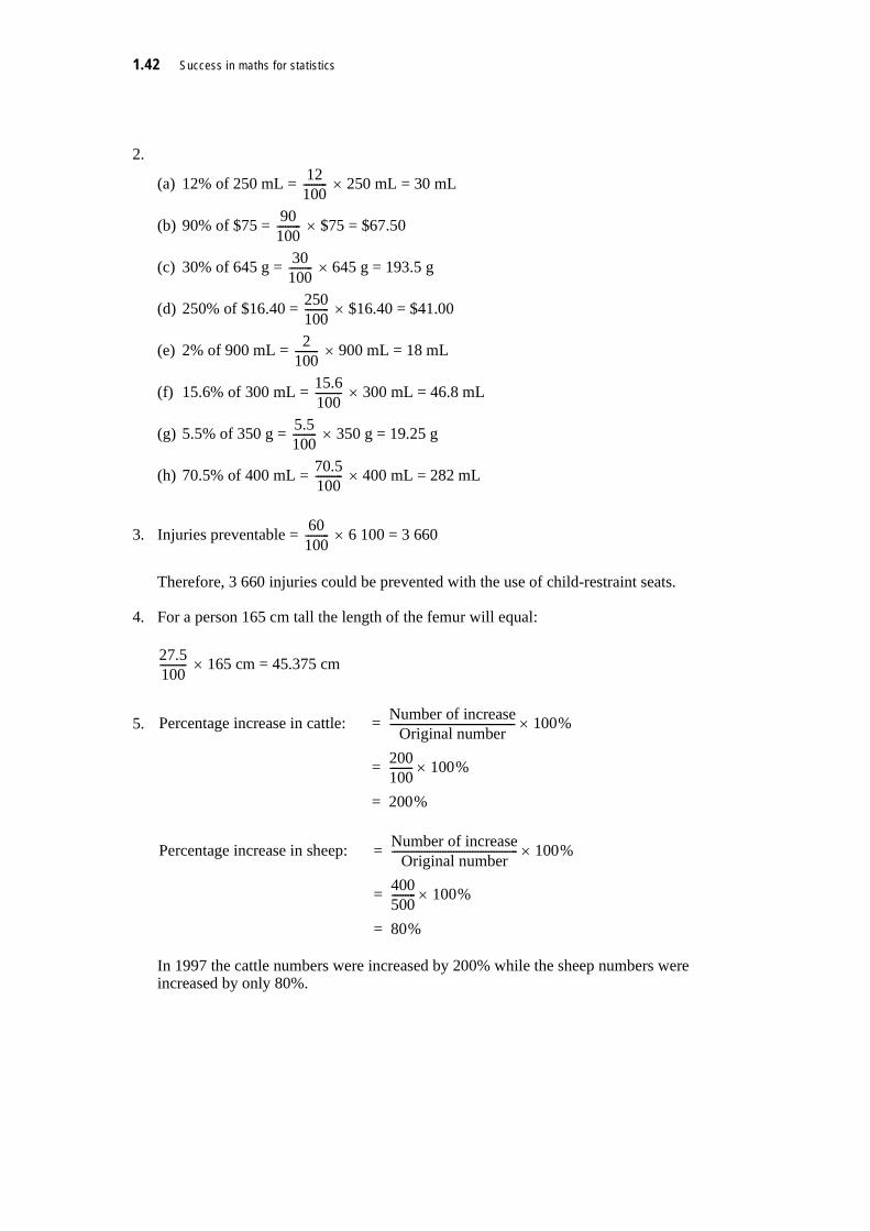
2.
(a) 12% of 250 mL = × 250 mL = 30 mL
(b) 90% of $75 = × $75 = $67.50
(c) 30% of 645 g = × 645 g = 193.5 g
(d) 250% of $16.40 = × $16.40 = $41.00
(e) 2% of 900 mL = × 900 mL = 18 mL
(f) 15.6% of 300 mL = × 300 mL = 46.8 mL
(g) 5.5% of 350 g = × 350 g = 19.25 g
(h) 70.5% of 400 mL = × 400 mL = 282 mL
3. Injuries preventable = × 6 100 = 3 660
Therefore, 3 660 injuries could be prevented with the use of child-restraint seats.
4. For a person 165 cm tall the length of the femur will equal:
× 165 cm = 45.375 cm
5.
In 1997 the cattle numbers were increased by 200% while the sheep numbers were increased by only 80%.
12100---------
90100---------
30100---------
250100---------
2100---------
15.6100----------
5.5100---------
70.5100----------
60100---------
27.5100----------
Percentage increase in cattle: Number of increaseOriginal number
----------------------------------------------- 100%×=
200100--------- 100%×=
200%=
Percentage increase in sheep: Number of increaseOriginal number
----------------------------------------------- 100%×=
400500--------- 100%×=
80%=

Module 2 – Formulas
Module 2
Formulas 2


Module 2 – Formulas 2.1
Aims
In Data Analysis we often generalise about and find relationships between data we collect. One of the best ways to show these relationships or generalisations is to use formulas. This module will revise some of the important rules when looking at formulas and look at how they can be applied in Data Analysis.
When you have successfully completed this module you should be able to:
• use mathematical formulas;
• rearrange and solve algebraic equations;
• develop and solve equations relating to practical situations.
2.1 Introduction
Consider the following sentences.
Gary once gave Gary’s wife a gift which Gary’s wife found so awful that Gary’s wife threw this gift in the bin. No matter how many times Gary asked Gary’s wife about the gift, Gary’s wife never mentioned the gift again.
It is very difficult to read as it stands. In English we replace many of these repeated words with pronouns (words that replace nouns). We are very familiar and comfortable with these words in everyday life. Using pronouns, the above sentences become much easier to read.
Gary once gave his wife a gift which she found so awful that she threw it in the bin. No matter how many times Gary asked his wife about it, she never mentioned it again.
Whenever we see she in the above text, we know that this refers to Gary’s wife, and whenever we see the word it we know it refers to the gift.
Let’s look at another sentence.
Shirley is always 3 years older than Jeffrey.
We can say that if Jeffrey is 4 years old then Shirley will be three years older than Jeffrey, meaning that Shirley is 7 years old. Or when Jeffrey is nineteen years old, Shirley will be three years older than Jeffrey, meaning that Shirley is twenty-two years old.
These sentences become hard to understand as were the sentences above. So in mathematics we introduce pronumerals to make the sentences easier to understand. Pronumerals and variables are the same thing. We will use the word variable throughout this module.
If we let S represent Shirley’s age in years and J represent Jeffrey’s age in years we know that the relationship between Jeffrey and Shirley is S = J + 3.

2.2 Success in maths for statistics
We can now rewrite the above sentences using variables (pronumerals) just as we re-wrote the original sentences using pronouns.
If J = 4, then S = J + 3, so S = 7. Or when J = 19, S = J + 3, so S = 22.
As long as we know what is meant by J and S we will understand these new sentences.
In Data Analysis, we use a variety of variables. For example, some variables are related to what they stand for: r stands for the regression coefficient; n stands for the sample size. Sometimes we wish to differentiate between variables that are similar, Here we often use subscripts. For example hA could stand for the heights of people in Asia and hE could stand for the heights of people in Europe. Other times we will use letters from the Greek alphabet. An α (alpha) is a common Greek variable used in statistics, as is β (beta) and sometimes χ (chi) although this is often written as X.
2.2 Simplifying expressions
This process of using letters to represent numbers is called algebra. The word algebra comes from the name of a book Al-jabr wa’l Muqabalah written by an Arabic mathematician, Al-Khowarizmi, in the early ninth century. The title of the book means something like ‘restoration and balancing’ and this will become an important part of solving and rearranging equations in this module.
Let’s look at some statements and their equivalent mathematical statements.
• The perimeter of a square is four times the length of one side.P = 4 × s where P represents the perimeter,P = 4s and s represents the length of one side.
• The bank charges 8% interest on my loan.I = 8% × A where I represents the interest charged on the loan in dollars,I = 8/100 × A and A represents the amount of the loan in dollars.I = 0.08 × A
• The adult weighed three times as much as the child.A = 3 × C where A represents the weight of the adult,A = 3C and C represents the weight of the child.
• The grevillea was half the height of the palm tree.G = 1/2P where G represents the height of the grevillea,
and P represents the height of the palm tree.
• The house was 15 metres longer than it was wide.L = W + 15 where L represents the length of the house,
and W represents the width of the house.
• To find the deviation from the mean, we subtract the mean from the value.D = x – where x is the value, and is the mean.
• Find the proportion of women who are less than 175 cm tall.p < 175 where p represents the proportion of women.
x x
Module 2 – Formulas 2.3
Remember that the letters we have used are called variables because they can vary to take on any value that we give them.
We can also call these formulas equations, because the expression on the left hand side (LHS) is equal to the expression on the right hand side (RHS).
Let’s look at some different examples.
Example
Write an equation to represent the following situation. Simplify the equation.
I think of a number and add 5. The result is 23.
Just as we define the variables when we write a formula, we must define the variables when we write an equation.
In this case we could say let N be the number I thought of.
Example
If Toby weighs three times as much as Harold, write an equation to represent the situation.
Here are some questions for you to do.
Activity 2.1
1. Write an equation to represent each of the following situations.
(a) A number plus 5 gives 35.
(b) A number minus 9 is equal to 2 times the same number.
(c) 6.5 times a number equals –3.4
(d) Five times a number gives 22.
2. Write an equation to represent each of the following situations.
(a) Ben is five times older than John.
(b) The length of the rectangle was 7 metres more than the width.
(c) Katie is five years younger than Jack.
(d) Barry earns one third the amount of money that Harry earns.
(e) The sample proportion is between 0.25 and 0.35
(f) At least 4 of the students are overweight.
Then, N + 5 = 23
T = 3 × H where T represents Toby’s weight,T = 3H and H represents Harold’s weight.

2.4 Success in maths for statistics
In the previous Activity you were required to write some equations. Just to remind you of the difference between expressions and equations. An expression might involve variables, numbers and symbols (+, –, ×, ÷, √, .....) but no equals sign. An equation on the other hand has an equals sign and indicates that two expressions are equal.
Example
Write an expression to represent the following situation and then simplify the expression.
Two times a number plus five times the same number.
We must define the variable. Let the unknown number be x
It is not necessary to include the multiplication sign, so we could rewrite this expression as:
We call 2x and 5x like terms because they contain the same power of the same variable. Similarly, 3x2 and 9x2 are like terms because they contain the same power of the same variable. The number in front of the variable, the coefficient, does not influence whether terms are like or not.
When we have like terms, we can apply the distributive law to simplify the expressions.
We could rewrite our expression as 7x
Let’s look a little more closely at like terms.
Examples
6a and 2a are like terms.
5x3 and –7x3 are also like terms because they have the same power of x, that is, x3. The coefficients, 5 and –7 do not influence our decision on like terms.
6x4 and 3y4 are not like terms because they contain different variables.
2x2 and 8x3 are not like terms because they have different powers of the same variable.
Example
Sort the following expressions into groups of like terms. 7x2, 5x, 3x2, 6x
We would group 7x2 and 3x2 together as like terms and 5x and 6x are like terms.
Then, 2 × x + 5 × x becomes the required expression.
2x + 5x
That is, 2x + 5x = 2 × x + 5 × x= (2 + 5)x applying the distributive law.= 7x
Module 2 – Formulas 2.5
Example
Simplify 3x + 2x
Are 3x + 2x like terms? Yes, because they have the same power of the same variable.
Example
Write an expression to represent the following situation, then simplify the expression.
Three times a number squared plus nine times the same number squared.
Let the number be x.
Example
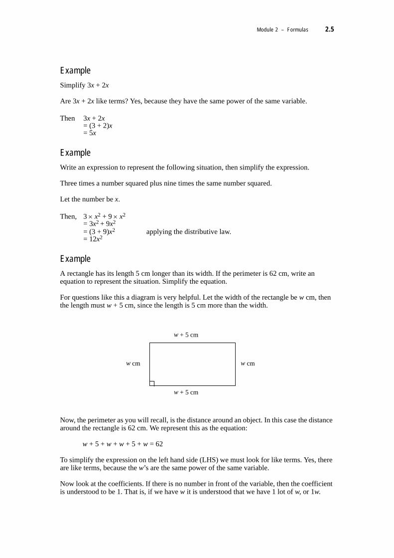
A rectangle has its length 5 cm longer than its width. If the perimeter is 62 cm, write an equation to represent the situation. Simplify the equation.
For questions like this a diagram is very helpful. Let the width of the rectangle be w cm, then the length must w + 5 cm, since the length is 5 cm more than the width.
Now, the perimeter as you will recall, is the distance around an object. In this case the distance around the rectangle is 62 cm. We represent this as the equation:
w + 5 + w + w + 5 + w = 62
To simplify the expression on the left hand side (LHS) we must look for like terms. Yes, there are like terms, because the w’s are the same power of the same variable.
Now look at the coefficients. If there is no number in front of the variable, then the coefficient is understood to be 1. That is, if we have w it is understood that we have 1 lot of w, or 1w.
Then 3x + 2x= (3 + 2)x= 5x
Then, 3 × x2 + 9 × x2 = 3x2 + 9x2
= (3 + 9)x2 applying the distributive law.= 12x2
w + 5 cm
w cmw cm
w + 5 cm

2.6 Success in maths for statistics
Let’s write our equation out with this new information.
On the LHS we can now group like terms.
Remember:
• You can only add or subtract like terms.
• If a term is just x, x2, etc., then the coefficient is one (that is, 1x and 1x2).
• Take care when regrouping terms with negatives.
Activity 2.2
1. Sort the following expressions 3x, 5a, 7a2, 6x2, 7x, 9a, 17x, 5x2, 6a2, 8x, 9x2, 12a, –4x, –11x2, –3a, –2x, 2a2 into groups of like terms.
2. Simplify the following expressions where possible.
(a) 5x + 6x
(b) 6x2 + 11x2
(c) x + 3x
(d) 7x – 3x
(e) 9x – 14x
(f) –8x – 4x
(g) –3.1x + –2.4x
(h) 4x + 32x – 7x
3. The length of a house is twice the width. If the perimeter of the house is 72 m write an equation to represent the situation. Simplify the equation.
4. A 75 metre long piece of rope is to be cut into two pieces. One piece is to be 15 metres longer than the other. Write an equation to represent the situation. Simplify the equation.
1w + 5 + 1w + 1w + 5 + 1w = 62
1w + 1w + 1w + 1w + 5 + 5 = 62 (1 + 1 + 1 + 1)w + (5 + 5) = 62 Using the distributive law
4w + 10 = 62 Simplifying.

Module 2 – Formulas 2.7
2.3 Relationships in words
This is probably the method of expressing a relationship that you are most familiar with at this stage.
For example,
• Chris earns twice as much as David.
• At the restaurant there are 5 more women than men.
• The bank charges 8% interest on my loan.
• The grevillea was half the height of the palm tree.
• The adult weighed three times as much as the child.
• The perimeter of a square is four times the length of one side.
• The house was 15 metres longer than it was wide.
While it is important that we are able to express in words what we are trying to find, it is more convenient to use a formula when we need to do some calculations using these relationships.
2.4 Relationships as formulas
We have already looked at expressing the relationship ‘Shirley is 3 years older than Jeffrey’ as a formula.
It is important if we are going to express our relationship as a formula using letters, that we know exactly what these letters represent. In our case, we have let S equal Shirley’s age in years and J equal Jeffrey’s age in years. We could have chosen any letters we liked but these two clearly help us to identify the required relationship. It is also important to note that it is not just Shirley and Jeffrey that we are comparing, but their ages. We should also note that their ages are always measured in years.
In this case we call S and J variables because they can vary to take on any values for S and J that we give them.
Let’s look at some of the word relationships from the previous section.
That is, S = J + 3 where S represents Shirley’s age in years, and J represents Jeffrey’s age in years.

2.8 Success in maths for statistics
Example
Translate the following relationship into a formula.
Chris earns twice as much as David.
What are the variables in this case?
...................................................................................................................................
You could have let the variables be C representing the amount of money that Chris earns and D representing the amount of money that David earns. Note that it is the amount of money that each earns that is the variable, not the person.
Before you go on to write a formula, think about the question. You know that Chris is the person earning the most money. Remove from the question any unnecessary words.
Put the symbol × for times.
C earns 2 × D
Finally put in the equals sign to form the formula.
It is an acceptable shorthand to leave the multiplication sign out of expressions involving variables. We say the multiplication is implied or understood.
So we could write C = 2D and we ‘know’ that we must multiply the 2 and the D.
Example
Translate the following relationship into a formula.
At the restaurant there are 5 more women than men.
We will firstly define the variables we will use.
Let W represent the number of women at the restaurant,and M represent the number of men at the restaurant.
To write the formula you could use one of two methods.
The ‘skeleton method’ where you could set up the skeleton of the formula with lots of room.
W = M
There are more women than men to we must add the 5 to the number of men to get the number of women.
W = M + 5
or,
Chris earns twice DavidC earns 2 times D
C = 2 × D where C represents the amount of money that Chris earns in dollars, and D represents the amount of money that David earns in dollars.
Module 2 – Formulas 2.9
The other method that you might use is to rearrange the question.
Example
Translate the following relationship into a formula.
The bank charges 8% interest on my loan.
The formula using one of the above methods, could be written:
We could also write this as I = 0.08A
Since it doesn’t matter which letters are chosen for variables in a formula (provided that it is understood what the letters mean) this formula could also be written as:
It is most important that the meaning of the variables be understood.
Formulas can involve two variables, just like the two examples above, but you might also see a relationship which involves only one variable and sometimes ones involving 3, 4 or more variables.
Example
The number of people in Toowoomba is approximately 90 000. We could write this as the formula
This is an example of a formula with one variable.
Five more women than men
or, Number of women is 5 more than number of men
Number of women is men plus 5
W is M plus 5
W = M + 5
I = 8% × A where I represents the interest charged on the loan in dollars,
I = × Aand A represents the amount of the loan in dollars.
I = 0.08 × A
y = 0.08x where y represents the interest charged on the loan in dollars, and x represents the amount of the loan in dollars.
N = 90 000 where N is the approximate population of Toowoomba.
8100---------

2.10 Success in maths for statistics
Example
The formula for finding the perimeter of a rectangle is
This is an example of a formula with three variables.
You might also notice that the formula for the perimeter of a rectangle contains two operations, namely addition and multiplication. The multiplication sign is understood to be after the 2, that is, P = 2 × (L + W)
In general, a formula can contain any number of different operations (addition, subtraction, multiplication, division, powers, square roots.......) depending on the relationship being described.
Activity 2.3
1. Express the following relationships as formulas.
(a) The distance (d) travelled be a car is equal to its speed (s) multiplied by the time (t) of the journey.
d =
(b) Profit (P) equals the revenue income (R) less the costs (C).
P =
(c) Electrical voltage (V) equals electrical current (I) times electrical resistance (R).
V =
2. Express the following relationships as formulas.
(a) The grevillea was half the height of the palm tree.(b) The adult weighed three times as much as the child.(c) The perimeter of a square is four times the length of one side.(d) The house was 15 metres longer than it was wide.
3. A shop stocks four times as many cola softdrink bottles as soda water. Write a formula to calculate the number of cola softdrink bottles given the number of soda water bottles.
4. If taxable income is greater than $33 500 in the Chook Islands, tax is calculated by subtracting $9 500 from the taxable income, then finding 39% of this difference, then adding $9 500. Write a formula to calculate the tax to be paid from the taxable income.
5. A small company pays their salesperson Mae Ihelpyu $200 per week plus $50 for each item that she sells in the week. Write a formula to calculate Mae’s weekly income for any number of items sold.
P = 2(L + W) where P represents the perimeter,L represents the length of the rectangle,
and W represents the width of the rectangle.

Module 2 – Formulas 2.11
2.5 Substituting into formulas
You will find that in subjects such as statistics, there are quite a lot of formulas. One of the main skills that are required of you, apart from determining which formula to use, is to be able to substitute values into a formula.
Recall our formula relating the ages of Shirley and Jeffrey.
By replacing the symbol for Jeffrey’s age with a numerical value I am able to find Shirley’s age.
When Jeffrey was 14 years old, how old was Shirley?
That is, when J = 14, what does S equal? We will substitute 14 for the J.
S = 14 + 3 = 17
So, when Jeffrey was 14 years old, Shirley was 17 years old. (Shirley is still 3 years older than Jeffrey as she always will be.)
Find Shirley’s age when Jeffrey is 19 and when he is 35.
You should have found that when Jeffrey is 19, Shirley is 22 and when he is 35, Shirley is 38.
Example
The formula for the area of a square is
When the length of the side of the square is 3 cm the area of the square will be
Find the area of a square with a side length of 9 cm.
S = J + 3 where S represents Shirley’s age in years, and J represents Jeffrey’s age in years.
A = s2 where A represents the area of the square, and s represents the side length of the square.
A = s2 = s × s= 3 cm × 3 cm Remember to multiply the units. cm × cm = cm2
= 9 cm2
A = s2
= s × s
= cm × cm
= cm2

2.12 Success in maths for statistics
Example
The formula for speed is
A giant tortoise can cover 100 metres in 20 minutes, what is the speed of the tortoise?
We need to be very careful with units when calculating speeds.
If a human can walk at about 4 km/h how does this compare to the giant tortoise?
We cannot compare the two speeds at the moment because they are in different units.
Convert the tortoises speed to km/h. .........................................................................
Did you get 0.3 km/h? (5 m/minute = 0.005 km/minute = 0.005 × 60 km/hour)
We can now see that the human can walk much faster than the tortoise. In fact, using our knowledge from the previous module, the human can walk more than 13 times faster than the tortoise.
Activity 2.4
1. The formula for the area of a rectangle is:
Find the area of the rectangle for the following lengths and widths.
2. In a square the perimeter is always 4 times the length of the side.
(a) Write this as a formula.
(b) Find the perimeter of squares with the following side lengths.
s = d/t where s represents speed,d represents the distance travelled,
and t represents the time taken.
s =
s =
s = 5 m/minute
A = lw Where l represents the length of the rectangle,and w represents the width of the rectangle.
(a) l = 7 cm w = 5 cm(b) l = 34 cm w = 21 cm(c) l = 3 m w = 67 m(d) l = 4 cm w = 82 mm
(i) 4 cm(ii) 7 m(iii) 2.6 mm(iv) 3/4 m
dt---
100 m20 minutes--------------------------

Module 2 – Formulas 2.13
(c) Suppose that you had a square chicken pen, of side length 3.2 metres. You wish to fence it with chicken wire costing $6.50 a metre. How much will it cost to fence the chicken pen?
3. The ratio of the circumference of a circle to its diameter is equal to π (Greek letter ‘pi). Another way to look at this is to say that the circumference is equal to π times the diameter.
(a) Write a formula that will allow us to find the circumference of the circle, given the diameter.
(b) Find the length of the circumference, rounded to one decimal place, for circles with the following diameters:
(c) Suppose that you have built a circular rose garden with diameter 3.8 metres in your yard. You wish to purchase a log type edging that comes in rolls of three metres costing $18.95 for roll. How many rolls of edging should you purchase, and what will be the cost?
4. If I stand on top of a cliff S metres high and drop a stone, it will take t seconds to reach the ground. The height of the cliff can be found using the following formula.
S = 4.9 t2
Use this formula to find the height of the cliff when it takes the following times for the stone to reach the ground.
(a) 3 seconds
(b) 8 seconds
(c) 1.4 seconds
5. Observation towers are often built in forests to allow bushfires to be spotted quickly. The distance (D) in kilometres that can be seen from a tower of height h metres is given by:
D =
Find the distance that can be seen from towers with the following heights. Round your answers to the nearest kilometre.
(a) 10 metres
(b) 25 metres
(c) 17.5 metres
(i) 3 cm(ii) 72 mm(iii) 6.5 m(iv) 3/5 m
8 h5---

2.14 Success in maths for statistics
6. We can quickly find the approximate area of skin on our body by using the following formula.
(a) This formula only gives approximate answers for average people. Explain why it wouldn’t be accurate for all people?
(b) Calculate the area of skin covering people with the following heights.
(c) If each of these people suffered burns to 24% of their bodies, calculate the area of skin that is burnt.
7. To check whether a person is the correct weight for their height, health workers now calculate the Body Mass Index. It is found by using the following formula.
For a person to be healthy their Body Mass Index should lie between 19 and 25 for a female and 20 to 26 for a male.
Calculate the Body Mass Index for the following people.
(a) Female, 165 cm, 65 kg
(b) Male, 178 cm, 85 kg
(c) Female, 150 cm, 75 kg
(d) you
Which of these people fall into the healthy category?
8. In statistics the formula for two sample t confidence interval is
calculate the t confidence interval when:
A = h2 where A represents the area of skin,and h represents the person’s height.
(i) 165 cm(ii) 175.5 cm(iii) 1.68 m
Body Mass Index = where w represents the weight in kilograms,and h represents the height in metres.
35---
wh2-----
2 21 2
1 21 2
( ) s sx x tn n
− ± +
1
2
1
2
1 2
1012
0.62.72.4
25
xxtssn n
==
=
=
== =

Module 2 – Formulas 2.15
2.6 Rearranging formulas
Occasionally we might be given the value of the subject of a formula and have to work out one of the other variables.
Let’s return to Shirley and Jeffrey.
We know that Shirley is three years older than Jeffrey and that this relationship is represented by the following formula or equation.
By replacing the symbol for Jeffrey’s age with a numerical value we are able to find Shirley’s age.
Supposing, however, that we knew Shirley’s age was 24 years and we had to work out Jeffrey’s age.
That is, when S = 24, what does J equal? In this case we could substitute 24 for S.
24 = J + 3
Then solve the equation. Alternatively we could re-arrange the formula we started with and make J the subject instead of S, after all in this question we want to find Jeffrey’s age!
Let’s look at a simpler example to begin with.
Example
If Adam’s age plus 4 equals 7, how old is Adam. (Pretend that you can’t work it out!)
Representing this as an equation we get:E
To find Adam’s age we must make A the subject of the equation. That is, we must get the A on its own.
Now an equation can be thought of as a balance, if we add or take something from one side we must do the same to the other or we will upset the balance.
S = J + 3 where S represents Shirley’s age in years,and J represents Jeffrey’s age in years.
A + 4 = 7 where A represents Adam’s age in years.
A A + 4 = 7

2.16 Success in maths for statistics
If we want to leave the A on its own we must remove the 4 that is with it. If we take the 4 from one side we must do the same to the other.
We are now left with:
We can now say that Adam must have been 3 years old.
Let’s just check that this is true.
We started by saying that:
and we rearranged (or solved) the equation:
to find that A = 3, or we found that Adam is 3 years old.
To check this answer we can substitute our answer into the original equation. We should look at the left and right hand sides of the equation separately.
The left hand side (LHS) of the equation becomes 3 + 4. We write this
We have rearranged the equation to make A the subject.
A + 4 = 7 where A represents Adam’s age in years.
A + 4 = 7A + 4 – 4 = 7 – 4 When working with equations, try to keep the
equals signs under each other.A = 3
LHS = 3 + 4 = 7= RHS Therefore our answer must be correct.
So, if A + 4 = 7then A = 3
A A + 4 – 4 = 7 – 4
A A = 3

Module 2 – Formulas 2.17
Let’s return to our original equation.
Example
We know that Shirley is three years older than Jeffrey and that Shirley is 24 years old. To find Jeffrey’s age we can rearrange our original formula so that J is the subject and then substitute into this.
To make J the subject we must get the J on its own. To do this we must remove the 3, but we must keep the balance by removing 3 from the other side of the equation as well. Since the 3 is added we must undo the addition be subtracting 3 from both sides.
Now if Shirley is 24 years old then:
Therefore Jeffrey is 21 years old, three years younger than Shirley as we would expect.
Alternatively we could have substituted S = 24 into the original formula and then solved for T.
Again we show that if Shirley is 24 years old, then Jeffrey must be 21 years old.
So far we have only looked at rearranging equations that involved addition or subtraction. Let’s look at some equations involving multiplication and division.
Example
The adult weighed three times as much as the child.
Now, what if we wanted to find the weight of the child given the weight of the adult? We will need to make C the subject of the equation. This time, the C is multiplied by the 3 so to remove the 3 we must do the opposite of multiplication, that is, division.
We must divide each side by 3.
S = J + 3 S – 3 = J + 3 – 3 Keep the equals signs under each other. S – 3 = J
J = S – 3 Writing the J on the left hand side of the equation.
J = S – 3J = 24 – 3J = 21
S = J + 324 = J + 3
24 – 3 = J + 3 – 321 = J
A = 3 × C where A represents the weight of the adult,A = 3C and C represents the weight of the child.

2.18 Success in maths for statistics
To find the age of the child we must divide the adult’s age by 3.
Example
Sometimes the formula that we are working with might have a number of variables to move. Consider the following equation that you would use in Data Analysis
(The symbols µ and σ are Greek letters and represent the mean and standard deviation of a group of numbers. You will learn more about this in Data Analysis.)
Supposing that we know z = 2, µ = 3 and σ = 0.8. To calculate the value of x we can either make x the subject and then substitute in the values or substitute the values into the formula and then solve it. We shall look at both methods.
Firstly we shall rearrange the formula to make x the subject.
In this example we have a division (÷ σ) and a subtraction (– µ) on the RHS.
Which do we attend to first?
Let’s think about what you would do if you knew a value for x.
If you were to substitute this value for x into the equation, you would firstly have to subtract µ and then divide by σ to get a value for z.
When rearranging equations we must do the opposite of these steps in the reverse order. We can think of this in terms of the following everyday occurrence.
Think of getting dressed. The first item/s of clothing you put on will be your underclothes (unless of course you are superman). This is followed by your outer clothing for the day, and finally a coat if necessary.
To undress at a later stage, instead of adding clothes you are taking them off. You also need to take off your clothes in the opposite order to that in which you put them on. That is, you remove the coat, then the outer clothes and finally your underclothes.
Recall the opposite of each operation.
That is, Cancel the 3’s on the top and bottom.
Writing the subject on the LHS.
A 3C=A3---
3C3-------=
A3--- C=
C A3---=
xz µσ−
=

Module 2 – Formulas 2.19
So for our example above to rearrange the equation we must multiply by and
then add µ.
Let’s look at this diagrammatically.
If you were to substitute a value for x into the equation, you would firstly have to subtract by µ and then divide by σ to get a value for y.
To rearrange the equation we must do the opposite of the above steps in the opposite order. Reading from right to left we have:
So in order to calculate our answer we then substitute z = 2, µ = 3 and σ = 0.8 into the rearranged formula shown above.
Operation Opposite+ –– +× ÷
÷ ×
xz µσ−
= σ

2.20 Success in maths for statistics
Alternatively we could have substituted the values into the original formula and solved (see below).
Lets consider another example.
Example
In the following formula find the value of x if we know that y = 2.3.
y = 8 – 4x
We can make x the subject of the following equation and then substitute into this y = 2.3.
You should note that when looking at equations or expressions, the sign in front of a number is the one attached to the number.
In the above example there is no sign in front of the 8 so it understood that this is positive 8. The sign in front of the 4x is negative so this is –4x.
Firstly we must think about what steps we would take if we knew a value for x and were trying to find a value for y.
In words, we have to multiply by –4 and then add 8. So to rearrange we would subtract 8 and then divide by –4.
Diagrammatically,
(multiplying both sides by 0.8)
(adding 3 to both sides)
x σz µ+=0.8 2 3+×=4.6=
z x µ–σ
------------=
2 x 3–0.8-----------=
2 0.8× x 3–0.8----------- 0.8×=
1.6 x 3–=1.6 3+ x 3– 3+=
4.6 x=
−4 × xxMultiply by −4 −4x + 8Add 8

Module 2 – Formulas 2.21
To rearrange the equation we must do the opposite of the above steps in the opposite order. Reading from right to left we have:
And algebraically,
y = 8 – 4x
y – 8 = 8 – 4x – 8 (subtracting 8 from both sides)
y – 8 = –4x
= (dividing both sides by –4)
= x
x = (writing the subject on the left hand side).
Now if we substitute y = 2.3 into this formula we obtain:
x = = 1.425
x Divide by −4 −4 × x Subtract 8 −4x + 8
y 8–4–----------- 4– x
4–---------
y 8–4–-----------
y 8–4–-----------
2.3 8–4–----------------

2.22 Success in maths for statistics
Activity 2.5
1. Rearrange the following equations to make the variable in the bracket the subject.
2. The perimeter of a square is four times the length of one side.
Rewrite this formula to make s the subject.
3. Before the invention of mechanical clocks, candles were used to measure the passage of time. A formula for the height of such a candle related to time is given below.
How long should it take before the height reaches 7.5cm? Use an equation to find this solution.
4. Economists have come up with the following formula relating the consumption of milk to the number of children in the family.
How many children should there be in a family if 18.5 litres of milk are used. To do this question rewrite the formula to make x the subject and then substitute.
5. In statistics a formula to find the margin of error is
In a situation we know that the standard deviation and . What sample size n must we use in order to have a margin of error of 0.28? Substitute these values into the formula and solve the corresponding equation.
s.
(a) R = 4a (a)(b) x + 2 = y (x)
(c) = k (b)
(d) y = 5x + 2 (x)(e) 7x – 8 = y (x)
(f) + 7 = s (t)
(g) = y (x)
P = 4 × s where P represents the perimeter,P = 4s and s represents the length of one side.
h = 10 – 2t where h equals the height of the candle in centimetres,and t equals the time in hours that the candle has been burning.
m = 3.5 + 2.5x where m is the number of litres of milk consumed per week,and x is the number of children in the family.
where z is the standard score, σ is the standard deviation and n is the sample size.
5b---
6t---
x 8+3------------
m zn
σ= ×
σ 0.8= z 2.1=

Module 2 – Formulas 2.23
Solutions
Activity 2.1
1.
2.
Activity 2.2
1. 3x; 7x; 17x; 8x; –4x; –2x
5a; 9a; 12a; –3a
7a2; 2a2; 6a2
6x2; 5x2; 9x2; –11x2
2.(a) 11x(b) 17x2
(c) 4x(d) 4x(e) –5x(f) –12x(g) –5.5x(h) 29x
3.
4.
(a) n + 5 = 35 where n represents a number(b) n – 9 = 2n(c) 6.5n = –3.4(d) 5n = 22
(a) B = 5J where B is Ben’s age and J is John’s age(b) L = W + 7 where L is the length and W is the width(c) K = J – 5 where K is Katie’s age and J is Jack’s age(d) B = J where B is Barry’s salary and J is Jack’s salary(e) 0.25 < p < 0.35 where p is the sample proportion(f) s ≥ 4 where s is the number of students
72 = 2(L + 0.5L) where L stands for the length of a house.= 2 (1.5 L)= 3L
75 = L + L + 15 where L stands for the shorter length of wire= 2L + 15
13---

2.24 Success in maths for statistics
ncome
Activity 2.3
Activity 2.4
1.(a) 35 cm2
(b) 714 cm2
(c) 201 cm2
(d) 3 280 mm2 or 328 cm2
2.(a) P = 4s(b)
3.(a) C = πd(b)
(c) Length = 11.93 m. So I need to buy 4 rolls. Cost = $18.95 × 4 = $75.80
4.(a) 44.1 m(b) 313.6 m(c) 9.604 m
5.(a) 11 km(b) 18 km(c) 15 km
(i) 16 cm(ii) 28 m(iii) 10.4 mm(iv) 3 m
(c) c = 3.2 × 4 × 6.5= $83.20
(i) 9.4 cm(ii) 226.2 mm(iii) 20.4 m(iv) 1.9 m
1. (a) (b) (c)
2. (a) 0.5 where is the height of the gravillea and is the height of the palm tree(b) 3 where is the height of the adult and is the weight of the
d stP R C
V IRG P G Pa x a x
== −==
= child(c) 4 where is the perimeter length and is the length of one side(d) 15 where is the length of the house and is the width
3. 4 where is the number of cola drinks an
p l p l x y x y
c s c
== +
= d is the number of soda drinks4. ( 9 500) 0.39 9 500 (if 33 500) where is the tax to be paid; is the taxable i5. 200 50 where is Mae's income and is the number of items sh
sT I I T II x I x
= − × + >= + e sells in a week

Module 2 – Formulas 2.25
6.
(a) not true for young babies since the ratio would be different(b)
(c)
7.(a) 23.9(b) 26.8(c) 33.3
8.
If we round these figures we would then say that we are confident the result is between –2.43 and –1.57.
Activity 2.5
1.
2.
(i) 16 335 sq cm(ii) 18 480.15 sq mm(iii) 1.693 sq m
(i) 3 920.4 sq cm(ii) 4 435.236 sq cm(iii) 0.406 4 sq m
( )2 22.7 2.410 12 0.6
25 252 0.6 0.5522 0.433 497 4041.566 502 596 or2.433 417 404
− ± +
= − ±= − ±= −
−
(a) 4
(b) 25(c)
2(d) 5
8(e) 7
6(f) t7
(g) 3 8
Ra
x y
bkyx
yx
sx y
=
= −
=
−=
+=
=−
= −
s P4---=

2.26 Success in maths for statistics
3. If we substitute h = 7.5 into the formula and then solve we obtain
So it must take 1.25 hours for the candle to reach 7.5cm.
4. If we rearrange the original formula we obtain . Substituting m = 18.5 into
this formula gives: . So there must be 6 children.
5. If we substitute , z = 2.1 and m = 0.28 into the original formula and solve we obtain:
(after subtracting 10 from both sides)
(after dividing both sides by –2)
(after multiplying both sides by )
(after dividing both sides by 0.28)
(after squaring both sides)
7.5 10 2t–=2.5– 2t–=
1.25 t=
x m 3.5–2.5-----------------=
x 18.5 3.5–2.5------------------------ 6= =
σ 0.8=
m z σn
-------×=
0.28 2.1 0.8n
-------×=
0.28 n 2.1 0.8×=
n 2.1 0.8×0.28---------------------=
6=n 36=
n

Module 3 – Graphing
Module 3
Graphing 3


Module 3 – Graphing 3.1
Aims
In Data Analysis you will need to be able to draw and interpret a number of different types of graphs. In this module we will revise some of the more important aspects of graphs.
When you have completed this module you should be able to:
• use the Cartesian Coordinate System to represent formulas;
• convert graphs and formulas into written descriptions;
• identify, draw and interpret linear graphs;
• predict the effects on linear graphs of changes to coefficients and constants in the equations;
• describe more complex graphs in words.
3.1 Describing a relationship from a graph
Graphs are a very convenient way to display information and it is up to the individual to interpret what the graph is ‘saying’. A well presented graph will be clear and easy to follow. It will have many important features:
• a heading describing what the graph is about;• clearly labelled horizontal and vertical axes;• scales on the axes;• lines or points plotted to indicate the relationship represented.
Example
Consider the following graph showing details of a Sunday drive.
A n A fte rn o o n d r iv e to a D is ta n t L o c a t io n
T im e
Dis
tanc
e fr
om h
ome
(km
)
0
2 0
4 0
6 0
8 0
1 0 0
1 2 0
1 4 0
1 6 0
1 :0 0 P M 2 :0 0 P M 3 :0 0 P M 4 :0 0 P M

3.2 Success in maths for statistics
When interpreting a graph we would firstly look at three items.
• The title is the first step. This should clearly tell us what the graph is about.
• Next look at the horizontal axis. In this case the axis represents time, from 1:00 pm to 4:00 pm.
• Finally look at the vertical axis. In this case the axis represents the distance from home in kilometres.
We should now have a clear picture on what the graph is about.
Next we look to the graph itself.
A series of questions might help you to clarify the meaning of the graph.
(a) At what time did the Sunday traveller leave home? ..................................................Did you say 1:00 pm? The distance from home at 1:00 pm was zero, so this is the time the traveller left home.
(b) At what time did the traveller reach their destination? ...............................................You should have said 4:00 pm.
(c) How far was the traveller from home when they reached their destination? ................They were 160 km from home.
(d) How far did the traveller go in the first hour? ..........................................................The first hour went from 1:00 pm to 2:00 pm and the distance from home at these times was 0 kilometres at 1:00 pm and 60 km at 2:00 pm. The distance travelled in the first hour was 60 kilometres.
(e) How far did the traveller go in the last hour? ............................................................Did you say 40 kilometres from 3:00 pm to 4:00 pm?
(f) What do you think happened between 1:30 and 1:45 pm? ...........................................What are your reasons for giving this answer? .......................................................................................................................................................................................You should have indicated that the traveller was stopped over this time period (or the traveller was lost and travelling in circles) because there was no change in the distance from home, it remained at 40 km.
(g) Over what other time period was the traveller stopped? ..............................................The graph indicates that the traveller was stopped between 2:45 and 3:30 pm.
(h) What was the total time spent travelling? ...................................................................This question requires you to do some calculations. The Sunday drive lasted for 3 hours but some of this time was spent not travelling. The total time spent travelling was 2 hours.

Module 3 – Graphing 3.3
Activity 3.1
1. The following graph shows the annual breeding numbers of loggerhead turtles at Mon Repos on the Bundaberg coast over about 20 years.
(a) In what year did the most turtles nest at Mon Repos?
(b) In what year was there the least number of turtles?
(c) Between which two years was there the greatest increase in turtle numbers?
(d) Between which two years was there the greatest decrease in turtle numbers?
(e) Scientists working in the Mon Repos area have predicted that this nesting sight will only last another 10 years if action is not taken. How do you think they might have come to this conclusion?
2. The following graph shows the age distribution of higher education students.
(a) What percentage of students in higher education in 1991 were aged 20–24 years?
(b) In which year did the 19 years and under group have the greatest representation in higher education?
(c) Which age group has the lowest representation in the higher education sector?
Annual Breeding Numbers of Loggerhead Turtlesbetween 1967 and 1993
Breeding Season
Tota
l Num
ber o
f Bre
edin
g Tu
rtle
s
0
100
200
300
400
500
600
700
1965 1970 1975 1980 1985 1990 1995

3.4 Success in maths for statistics
(Source: Selected Higher Education Student Statistics, DEET.)
3. Following are two graphs showing how a beetle travelled over a set distance. The first graph shows the distance the beetle walked over a given time. The second graph shows the speed at which the beetle was travelling at any particular time.
(a) Between which times is the beetle not moving? Explain how this is reflected in both graphs.
(b) From the first graph determine how far the beetle travelled between 0 and 1 minutes.
(c) From the second graph determine how fast the beetle travelled between 0 and 1 minutes. Can you see how this speed was calculated?
Age distribution of Higher Education Students 1985 - 1995
Year
Perc
enta
ge
10
15
20
25
30
35
40
1985 1987 1989 1991 1993 1995
19 years and under20 - 24 years25 - 29 years30 years and over
Distance travelled by Beetle (metres)
Time (minutes)
Dis
tanc
e (m
etre
s)
0
2
4
6
8
10
12
0 1 2 3 4
Speed of Beetle (metres/minute)
Time (minutes)
Spee
d (m
etre
s pe
r min
ute)
0
5
10
0 1 2 3 4

Module 3 – Graphing 3.5
Recall from earlier in this module we gave the formula for speed as:
Speed = distance/time
From the first graph you found that the beetle covered 5 metres in the first minute.
That is: , which is the speed
you found from the second graph.
(d) From the first graph, calculate the speed at which the beetle travelled between 3.5 and 4 minutes. Mark this on the second graph.
4. The following graph shows the time it takes to run a race plotted against the distance over which the race was run.
Look at this graph carefully until you understand what relationship the graph is describing. Write a sentence explaining what is wrong with this graph.
5. The following graph is from a Data Analysis text (Moore 1996 p. 243)
The behaviour of the proportion of tosses that give a head,from 1 to 1000 tosses of a coin.
speed distancetime------------------- 5 m
1 minute--------------------- 5 m/minute= = =
Time against distance for a foot race
01234567
0 1 2 3 4Length of race (km)
Tim
e fo
r rac
e (m
inut
es)

3.6 Success in maths for statistics
What do you notice about the scale on the horizontal axis? You will find that it does not go up evenly, in fact it goes up in powers of 10 (the distance from 1 to 10 is the same as the distance from 10 to 100) This is called a log scale. It is used when there are large numbers on one or both of the scales. Write a few sentences describing the graph.
6. The graph below is from a Data Analysis text (Moore 1996, p. 292)
The distribution of returns for New York Stock Exchange commonstocks since 1987
Write a few sentences describing the graph.
3.2 Relationships as graphs
You have probably used a map at some stage to find the location of a particular place. Map makers commonly set up a grid to allow you to do this. They use a letter to label a column and a number for a row (this will sometimes vary).
Look at the map of the University of Southern Queensland on the next page. Suppose you were looking for the Library and were given the grid reference J7. To find it you need to go across to column J and from there go up or down to row 7. The library will be found at this point. (It is actually labelled R on the map.)
Now find the new Office of Preparatory and Continuing Studies, the grid reference being K8. Go across to K and then up or down to 8. You should have found it labelled S on the map. If you are ever in Toowoomba call into S and say hello to us.

Module 3 – Graphing 3.7
Activity 3.2
1. What is located at the following grid references.
(a) I6(b) D5(c) N7
2. Find the grid reference for the following places.
(a) Steele Rudd Courts.(b) W Block Sciences (nursing and psychology) and Shopping Complex.(c) Gymnasium
Obviously a grid system is a very useful tool because everyone agrees on the location of a particular point.
Mathematicians use a similar system to refer to a point in a plane (a flat surface extending infinitely in all directions) and to distinguish it from any other points in that plane.
The system we use today was developed by a seventeenth century mathematician called René Descartes. Legend has it that the idea of coordinates came to him while he lay in bed and watched a fly crawling on the ceiling. Noting that each position of the fly could be expressed by two distances from the edges of the ceiling where the walls and ceiling met. He set up a grid using two number lines at right angles. The horizontal number line is usually called the x-axis and the vertical number line is usually called the y-axis. In fact these horizontal and vertical number lines can have any name as you will see as we move through this module. These two axes (the plural of axis and pronounced ax/ees) meet or intersect at a point called the origin. We call this grid system the Cartesian Coordinate System after its inventor.
3.2.1 The Cartesian plane
A Cartesian plane would look like this.
In this case I have labelled the axes x and y as you will often see, but I could also have labelled them J and S, or any other variable that I wish to represent.
x
y
Origin
x-axisy-axis

3.8 Success in maths for statistics
As each axis is a number line it must have a scale drawn on it as we have done before when constructing a number line. The numbers extend out infinitely in either direction from the origin. All the way along the axis one centimetre must always represent the same number of units. It is not necessary to have the same scale on both axes although this will often be the case.

Module 3 – Graphing 3.9
Look at the following Cartesian planes where different scales have been used. Note that only one scale has been used per axis. With a ruler, check that the scales are correct on each axis.
You will also have noticed that the two axes divide the plane into four regions. We call these regions quadrants. They are numbered as in the following diagram.
Any point can be represented on the Cartesian plane by using a pair of numbers that we call an ordered pair. To describe a point we give its horizontal or x-coordinate and its vertical or y-coordinate. This pair of numbers is always written in strict order, stating the x-coordinate first followed by the y-coordinate.
That is (x-coordinate , y-coordinate)
We abbreviate this to be (x , y)
Or, if we are not using x and y as our variables then in general we give the horizontal coordinate first and the vertical co-ordinate second.
That is (horizontal coordinate , vertical coordinate)
Let’s now look at using this scheme to locate some points on the Cartesian plane.
To locate the point (3,2) firstly establish which is the x-coordinate and which is the
y-coordinate. As ordered pairs are always in the form (x,y) we know that the x-coordinate is 3 and the y-coordinate is 2.
The same scale isused on each axis
Different scales areused on each axis
Different scales areused on each axis
−3 −2 −1 0 1 2 3
−2
−1
1
2
x
y
−3 −2 −1 0 1 2 3
−10
−5
5
10
x
y
−0.3 −0.2 −0.1 0 0.1 0.2 0.3
−200
−100
100
200
x
y
x
y
Quadrant 1Quadrant 2
Quadrant 3 Quadrant 4

3.10 Success in maths for statistics
Having drawn a Cartesian plane, go across to 3 on the x-axis and up to 2 on the y-axis.
The dotted lines have been drawn to help you locate the point. These are only for guidance and would not normally be included on your diagram.
The point (3,2) lies in the first quadrant. We can locate points in other quadrants using the same technique.
Let’s plot the point (–1,2). Again we must firstly determine that the x-coordinate is –1 and the y-coordinate is 2. This time we must move left from the origin to get to –1 and then up to 2 on the y-axis. You will notice that this point is in the second quadrant.
−4 −3 −2 −1 0 1 2 3 4
−4
−3
−2
−1
1
2
3
4
x
y
(3,2)
−4 −3 −2 −1 0 1 2 3 4
−4
−3
−2
−1
1
2
3
4
x
y
(−1,2)
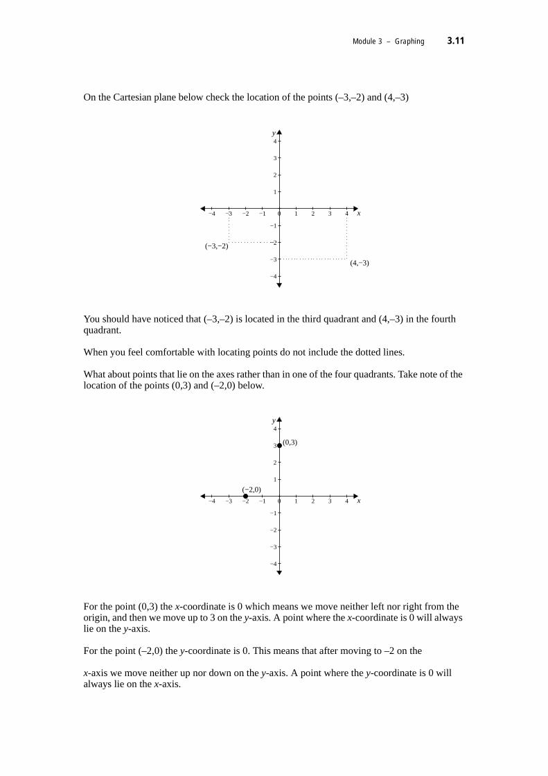
Module 3 – Graphing 3.11
On the Cartesian plane below check the location of the points (–3,–2) and (4,–3)
You should have noticed that (–3,–2) is located in the third quadrant and (4,–3) in the fourth quadrant.
When you feel comfortable with locating points do not include the dotted lines.
What about points that lie on the axes rather than in one of the four quadrants. Take note of the location of the points (0,3) and (–2,0) below.
For the point (0,3) the x-coordinate is 0 which means we move neither left nor right from the origin, and then we move up to 3 on the y-axis. A point where the x-coordinate is 0 will always lie on the y-axis.
For the point (–2,0) the y-coordinate is 0. This means that after moving to –2 on the
x-axis we move neither up nor down on the y-axis. A point where the y-coordinate is 0 will always lie on the x-axis.
−4 −3 −2 −1 0 1 2 3 4
−4
−3
−2
−1
1
2
3
4
x
y
(4,−3)
(−3,−2)
−4 −3 −2 −1 0 1 2 3 4
−4
−3
−2
−1
1
2
3
4
x
y
(0,3)
(−2,0)

3.12 Success in maths for statistics
Activity 3.3
1. In Data Analysis you will be studying ‘regression’ which will require you to plot sets of ordered pairs that are related. The example below compares the household spending on tobacco products and alcoholic beverages in Great Britain.
Plot the points on a Cartesian plane.
2. Another graph that is used in Data Analysis is called a ‘residual plot’. Here we look at a model of what is predicted and we plot the difference between the observed and the predicted values. Below are the speeds of a British Ford Escort and the difference between the observed mileage and predicted mileage (e.g. at 10km/hr the mileage is 21 litres/100km but the predicted was 31.9 litres/100 km, so the difference is 10.9). Plot the information below.
Household Tobacco Alcohol1 2.6 4.72 2.9 4.53 3.2 5.94 3.3 4.85 3.5 5.66 3.7 6.27 3.8 6.38 4.1 6.59 4.5 6.2
10 4.6 411 3.6 5.3
Speed (km/hr)
Observed – Predicted Speed80
Observed – predicted–2.94
10 10.9 90 –2.1720 2.24 100 –1.3230 –0.62 110 –0.4240 –2.47 120 0.5750 –3.33 130 1.6460 –4.28 140 2.7670 –3.73 150 3.97
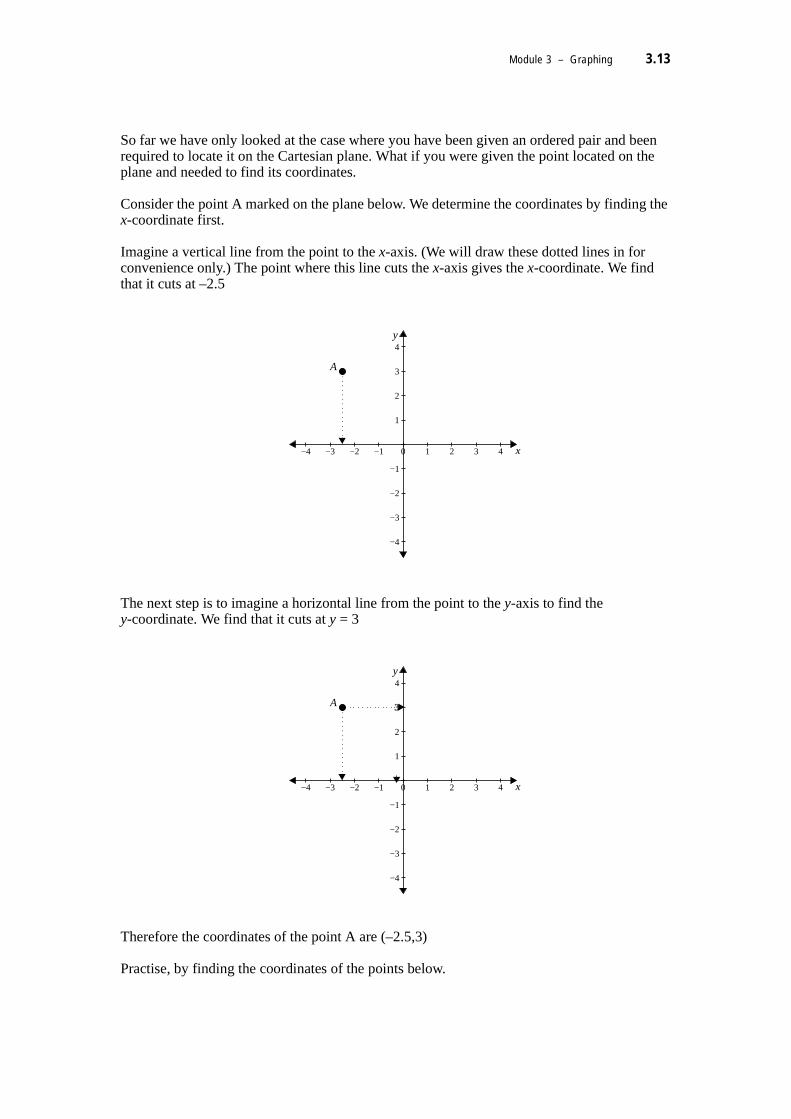
Module 3 – Graphing 3.13
So far we have only looked at the case where you have been given an ordered pair and been required to locate it on the Cartesian plane. What if you were given the point located on the plane and needed to find its coordinates.
Consider the point A marked on the plane below. We determine the coordinates by finding the x-coordinate first.
Imagine a vertical line from the point to the x-axis. (We will draw these dotted lines in for convenience only.) The point where this line cuts the x-axis gives the x-coordinate. We find that it cuts at –2.5
The next step is to imagine a horizontal line from the point to the y-axis to find the y-coordinate. We find that it cuts at y = 3
Therefore the coordinates of the point A are (–2.5,3)
Practise, by finding the coordinates of the points below.
−4 −3 −2 −1 0 1 2 3 4
−4
−3
−2
−1
1
2
3
4
x
y
A
−4 −3 −2 −1 0 1 2 3 4
−4
−3
−2
−1
1
2
3
4
x
y
A 3

3.14 Success in maths for statistics
Activity 3.4
Find the coordinates of the points marked on the Cartesian plane below.
Let’s summarise what we have learned about the points located in the various quadrants.
-5
-4
-3
-2
-1
0
1
2
3
4
5
-5 -4 -3 -2 -1 0 1 2 3 4 5
(d)
(a)(b)
(c)
(g)
(f)
(e)
x
y
Quadrant 1
x-coordinate positive, y-coordinate positive
(+,+)
Quadrant 2
x-coordinate negative, y-coordinate positive
(−,+)
Quadrant 3
x-coordinate negative, y-coordinate negative
(−,−)
Quadrant 4
x-coordinate positive, y-coordinate negative
(+,−)

Module 3 – Graphing 3.15
3.2.2 Drawing graphs
The general purpose of a graph is to give a visual representation of the relationship between two or more things. Graphs must contain clear, precise and meaningful information for the reader.
This section takes you step by step through the process of drawing a graph by plotting points. This is only one of many ways to develop a graph, but it is one that you can always fall back on, no matter what the shape of the graph. In this section we are only going to look at straight line graphs.
For this section you will need to have some 2 mm graph paper so that you can practise drawing graphs and reading off accurate answers. It is also helpful to have a well sharpened pencil to draw the graphs. You should draw the graphs on graph paper as we move through the steps.
Suppose there is a brother and sister Shirley and Jeffrey. Shirley is three years older than Jeffrey. This can be represented by the formula.
Using the Cartesian coordinate system, if we could find a number of ordered pairs, we could locate these on the Cartesian plane and join them up to get a graph of this relationship.
When Jeffrey was 14, Shirley was 17When Jeffrey was 19, Shirley was 22When Jeffrey was 35, Shirley was 38
A convenient way to represent this information is to enter it in a table of values.
From our table of values we can write a series of ordered pairs that satisfy the formula.
In each case Jeffrey’s age (horizontal axis) comes first and Shirley’s age (vertical axis) is second.
The series of ordered pairs can now be plotted on a Cartesian plane so that we can see the relationship between Jeffrey’s age and Shirley’s age.
Before we draw our axes let’s think about the possible values for the ages. Since neither Jeffrey’s age nor Shirley’s age can be negative we are only interested in the first quadrant.
S = J + 3 where S represents Shirley’s age in years,and J represents Jeffrey’s age in years.
Jeffrey 14 19 35Shirley 17 22 38
(14,17) (19,22) (35,38)

3.16 Success in maths for statistics
Now choose an appropriate scale to suit the ordered pairs. In our table of values, the maximum value for Shirley’s age is 38 and for Jeffrey, 35. Let’s then make the axis for Shirley’s age go up to 40 and for Jeffrey’s to 35.
Now plot the ordered pairs on the Cartesian plane drawn.
Jeffrey's Age (years)
Shir
ley'
s Age
(yea
rs)
Note: Axes are labelled J and S andgiven word labels because the graph isshowing a specific relationship.
Jeffrey's Age (years)
Shir
ley'
s Age
(yea
rs)
0
5
10
15
20
25
30
35
40
0 5 10 15 20 25 30 35

Module 3 – Graphing 3.17
To illustrate the trend in the graph we draw a straight line through all of the plotted points. When drawing a trend line we need to think about whether all values on the x-axis are possible. In our case we are talking about ages in years. We can have 5 years, 10 years and so on, as marked on the graph, but we could also have 5 ½ years, or 6 years, 3 months and 4 days, so yes all values are possible on the x-axis. Since all values are possible we will draw a solid line when joining the plotted points.
Finally give the graph a title.
Notice that we do not stop at the points we have plotted when drawing in the trend line. The points we have plotted were only three of an infinite number of possibilities.
Jeffrey's age (years)
Shirl
ey's
age
(yea
rs)
0
5
10
15
20
25
30
35
40
0 5 10 15 20 25 30 35
Ages of Shirley and Jeffrey
Jeffrey's age (years)
Shirl
ey's
age
(yea
rs)
0
5
10
15
20
25
30
35
40
0 5 10 15 20 25 30 35

3.18 Success in maths for statistics
Once the graph is drawn it is easy to read off Shirley’s age for any age of Jeffrey.
When Jeffrey was 15, Shirley was 18. This is not easy to find on the above graph, but having drawn yours on 2 mm graph paper you should be able to read off your answer fairly accurately.
Let’s now summarise the steps we have taken to draw a graph.
• From the formula complete a table of values.
• Draw up a Cartesian plane and label the axes (don’t forget the units if appropriate).
• Choose a suitable scale.
• Plot the ordered pairs from the table of values.
• Draw a trend line extending through and beyond the plotted points.
• Give your graph a title.
Let’s now look at another example, following the same steps as last time.
Example
A small company pays their salesperson Mae Ihelpyu $200 per week plus $50 for each item that she sells in the week. Write a formula to calculate Mae’s weekly income for any number of items sold.
The formula required was:
If you were to graph this formula you could find the total income for Mae selling any number of items in a given week. Or, given a set amount of money to be earned in one week, we could calculate the number of items to be sold.
Can you see that the amount of money Mae earns depends on the number of items she sells?
I = 200 + 50n where I represents the total income in dollars,and n represents the number of items sold.
Ages of Shirley and Jeffrey
Jeffrey's age (years)
Shirl
ey's
age
(yea
rs)
0
5
10
15
20
25
30
35
40
0 5 10 15 20 25 30 35

Module 3 – Graphing 3.19
We call Mae’s income the dependent variable because it depends on the number of items she sells, and we call the number of items sold the independent variable because this can be any number of items.
It is usual to put the independent variable first in the table of values.
Complete the following table of values.
Completing the table of values we have:
Now draw up the Cartesian plane and label the axes. Again we only require the first quadrant as the number of items sold can only be positive and the total cost must also be positive.
Now choose a suitable scale. The horizontal axis (number of items sold) will need to start at zero, the minimum number of items that could be sold. The vertical axis though, could start at $100, a number just smaller than the least amount earned, which is $200. If we do not start the scale on an axis at zero, we should indicate that we have not started at zero.
Number of Items sold (n) 0 5 10Total Income in $ (I)
When n = 0 When n = 5 When n = 10
I = 200 + 50n I = 200 + 50n I = 200 + 50n= 200 + 50 × 0 = 200 + 50 × 5 = 200 + 50 × 10= 200 + 0 = 200 + 250 = 200 + 500= 200 = 450 = 700
Number of Items sold (n) 0 5 10Total Income in $ (I) 200 450 700
Number of items soldn
C
Total Income ($)

3.20 Success in maths for statistics
Now plot the ordered pairs from the table of values
Again the independent variable comes first and is the one plotted on the x-axis.
Before drawing a trend line through the points, we need to think about whether all values on the x-axis are possible. In this case we are talking about number of items sold. We can have 5 items sold, 10 items sold and so on, as marked on the graph, but in this case we could not have 5½ items sold (who wants to buy, say, 1/2 a TV?). So this time, all values are not possible on the x-axis. Since all values are not possible we will draw a dotted or broken line when joining the plotted points.
Finally give your graph a title.
Total Income for any given number of Items Sold
Let’s now read off some values from your graph. These are not easy to find on the above graph, but having drawn yours on 2 mm graph paper you should be able to read off your answers fairly accurately.
(0,200) (5,450) (10,700)
Number SoldT
otal
Inco
me
($)
100
300
500
700
900
1100
0 5 10 15 20
This is the mark toindicate that the y-axisdidn’t start at zero.
Number sold
Tota
l Inc
ome
($)
100
300
500
700
900
1100
0 5 10 15 20

Module 3 – Graphing 3.21
What would Mae earn if she sold 7 items in one week? ..........................................
How many items would Mae have to sell to earn $600 in a week? ...........................
You should have found that Mae earned $550 for selling 7 items, and to earn $600 would need to sell 8 items.
You could check these answers by substituting them into the formula.
Example
Let’s finally look at a graph from a statistical equation called the regression line. An equation is just another name for a formula. It is looking at the relationship between two variables as before. For example a university in the US conducted a study on the relationships between the average temperature (°F) during the month babies started to crawl and the baby’s age. They found a relationship in the form of an equation:
y = –0.08x + 35.7
To sketch the graph of the formula, we follow the same steps as before.
The first thing to calculate is a table of values. You will need to decide what x values you will choose to put into your table. In this example there would be no negative values. The temperature range would be about 30° to 100° F.
Now complete the table of values.
The ordered pairs that we will plot are:
Plot the points, draw a line through and beyond the points. Finally label your graph.
When n = 7 When n = 8I = 200 + 50n I = 200 + 50n
= 200 + 50 × 7 = 200 + 50 × 8= 200 + 350 = 200 + 400= 550 = 600
x 30° 50° 90°y
When x = 30 When x = 50 When x = 90
y = –0.08x + 35.7 y = –0.08x + 35.7 y = –0.08x + 35.7= –0.08 × 30 + 35.7 = –0.08 × 50 + 35.7 = –0.08 × 90 + 35.7= 33.3 = 31.7 = 28.5
x 30° 50° 90°y 33.3 31.7 28.5
(30,33.3) (50,31.7) (90,28.5)

3.22 Success in maths for statistics
Activity 3.5
To complete this Activity you will need graph paper.
1. Before the invention of mechanical clocks, candles were sometimes used to measure the passage of time. A formula for the height of such a candle related to time is given below.
h = 10 – 2t
where h equals the height of the candle in centimetres, and t equals the time in hours that the candle has been burning.
(a) Use this formula to complete the following table.
(b) Graph this formula, letting the horizontal axis represent time.
(c) What was the height of the candle before it was lit?
(d) What does the 10 represent in the formula?
(e) For how many hours will the candle burn?
2. Suppose that you were planning a holiday in the United States. You wanted to know what clothes you should take so you looked up the expected temperatures in the newspaper. Problem is the temperatures were in degrees Fahrenheit and you never knew or have long forgotten what this means. A conversion graph will be useful to convert between degrees Fahrenheit and degrees Celsius.
(a) Draw a graph for the following information. You will need a full page graph with careful choice of scales to be able to read off accurate answers.
t 0 1 2 3 4 5h
Degrees Celsius (°C) 0 10 20 40 80 100Degrees Fahrenheit (°F) 32 50 68 104 176 212
Regression line of crawling age on temperature
28303234
0 20 40 60 80 100
temperature (degrees F)

Module 3 – Graphing 3.23
(b) If you had found that the average temperature in the month you were planning to visit the USA was 59°F, what would this be in degrees Celsius?
(c) If it was 35°C in Australia, what would this be in degrees Fahrenheit?
3. The Leaky Boat Company hires out paddle boats for $7.50 an hour.
(a) Develop a formula relating the time you have the boat to the total cost of the hire. Don’t forget to define your variables.
(b) Complete the following table of values.
(c) Draw a graph showing the time you have the boat against the cost of the hire.
(d) If a family decides to hire the boat for 4 hours in the morning, what will be the cost of the boat?
(e) If another family comes to hire the boat for the afternoon but only has $24, for how many hours will they be able to hire the boat?
4. A car rental company charges an initial fee of $50 per day plus 15 cents per kilometre.
(a) Write a formula relating the kilometres travelled to the total cost for a days rental. Don’t forget to define the variables.
(b) Draw up a table of values and construct a graph to represent this relationship.
(c) From your graph, determine the cost of renting the car for one day and driving 260 kilometres.
(d) If you had $110 to spend, how many kilometres could you travel in one day?
5. The amount of time that you can spend in the sun without burning is related to the sun protection factor (SPF) of the sunscreen lotion you use. The table below is for a person who can stay in the sun without any lotion for only 15 minutes without burning.
(a) How does the increasing of the sunscreen factor by 2 change the time that can be spent in the sun?
(b) Draw a graph of this relationship.
(c) If this person wanted to stay in the sun for 1 hour without burning, what is the minimum sunscreen factor that would be required?
Number of Hours 1 2 3 5 8Total Cost ($)
Sunscreen Factor 8 10 12 14Time in minutes 120 150 180 210

3.24 Success in maths for statistics
6. The regression equation: y = –1.03 + 0.206x, shows the relationship between increase in cigarette consumption and change in nicotine yields. x is the variable reduction in nicotine yield (%), and y is the variable increase in cigarette consumption (%).
(a) Draw a graph showing this relationship
(b) A 50% reduction in nicotine yield might produce a rise in cigarette consumption of _________%
(c) A person changed from cigarettes containing 2.1 mg of nicotine to ones that contained 1.3 mg. What increase in consumption would you expect?
3.3 Gradients of line graphs
Consider the following graph, showing the annual breeding numbers of loggerhead turtles at Mon Repos on the Bundaberg coast over about 20 years.
Part of this graph, from 1967 up to 1974 is enlarged and reproduced below.
Annual Breeding Numbers ofLoggerhead Turtles between 1967 and
1993
Breeding Season
Tota
l Num
ber o
f Bre
edin
g Tu
rtle
s
0
100
200
300
400
500
600
700
1965 1970 1975 1980 1985 1990 1995

Module 3 – Graphing 3.25
What was the increase in breeding numbers between 1969 and 1970? .....................What was the increase in breeding numbers between 1972 and 1973? .....................
Between 1969 and 1970 turtle numbers increased by about 60, while between 1972 and 1973 numbers increased by about 220.
What do you notice about the steepness of the graph between 1969 and 1970 and between 1972 and 1973? ..................................................................................
Did you say that the graph is steeper over the second period?
Let’s look more closely at these two results. We will look at an even smaller part of the graph this time.
Over the 1 year period between 1969 and 1970 the number of turtles rose by 60.
Annual Breeding Numbers of Loggerhead Turtlesbetween 1967 and 1974
Breeding Season
Tota
l Num
ber o
f Bre
edin
g Tu
rtle
s
0
100
200
300
400
500
600
700
1967 1968 1969 1970 1971 1972 1973 1974
Increase of 60breeding turtles
1 year

3.26 Success in maths for statistics
Between 1972 and 1973, again a 1 year period, the number of turtles rose by 220.
Imagine walking up these two ‘hills’. It would be hard work climbing up the second much steeper ‘hill’. We say that the second of our diagrams has a much greater slope than the first diagram. Another word for the steepness or slope of a line is to talk of its gradient.
In fact we can put a value on the steepness or gradient of the line, by putting the value for the change in height over the change in horizontal distance.
That is,
You might also see this written as:
This formula means exactly the same thing as the formula above.
Let’s find the gradients of the two lines taken from our graph above.
Over the 1 year period between 1969 and 1970 the number of turtles rose by 60.
We can say that the rate of change in turtle numbers over this period was 60 turtles per year.
increase of 220breeding turtles
1 year
gradient change in heightchange in horizontal distance----------------------------------------------------------------------=
gradient riserun--------=
gradient change in heightchange in horizontal distance----------------------------------------------------------------------=
gradient 601------ 60= =
increase of 60breeding turtles
1 year

Module 3 – Graphing 3.27
Between 1972 and 1973, again a 1 year period, the number of turtles rose by 220.
Similarly we can say that the rate of change in turtle numbers over this period was 220 turtles per year.
So, the gradient of the graph between 1969 and 1970 is 60 while the gradient of the graph between 1972 and 1973 is 220. It can be seen from these figures that the gradient of the second part of the graph is much steeper than the gradient of the first part of the graph.
Let’s now look at some other examples of gradients.
Example
Find the gradients of the following line segment. A line segment is just a part of a line.
What the gradient is telling us is that for every 8 metres we move along in a horizontal distance, the vertical distance rises by 2 metres. We could also say that for every 4 metres in a horizontal direction we rise 1 metre. You may see engineers refer to this as a gradient of 1:4 using ratios as we have done in a previous module. If this was your block of land with this slope, the builder, the surveyor and the engineer would all be interested in the gradient of the block of land. If the land is too steep then slippage of the land could occur once the soil is disturbed. If the land is too steep there would need to be a deep cut in the land to make a level piece of ground on which to situate a concrete slab based house. This might mean that alternative methods of construction need to be considered.
In fact the building code prevents anyone building on land with a gradient greater than 1:4 due to the danger of land slippage.
Let’s return to our turtles at Mon Repos. This time we are only going to look at that part of the graph from 1987 to 1993.
gradient change in heightchange in horizontal distance----------------------------------------------------------------------=
gradient 2201--------- 220= =
increase of 220breeding turtles
1 year
gradient change in heightchange in horizontal distance----------------------------------------------------------------------=
gradient 28---
14---= =
8 m
2 m

3.28 Success in maths for statistics
What was happening to the turtle numbers for the periods 1988 to 1989 and from 1991 to 1992?
.........................................................................................................................................
You should have said that the turtle numbers were decreasing.
Have a look at the two sections of graph for the above periods. How do they differ from the two periods that we looked at previously?
.........................................................................................................................................
This time the two segments of graph are falling as we move along the graph from left to right.
Annual Breeding Numbers of Loggerhead Turtlesbetween 1987 and 1993
Breeding Season
Tota
l Num
ber o
f Bre
edin
g Tu
rtle
s
0
50
100
150
200
250
300
1987 1988 1989 1990 1991 1992 1993
decrease of 70breeding turtles
1 year
1988–1989
decrease of 10breeding turtles
1 year
1991–1992

Module 3 – Graphing 3.29
To distinguish a graph that is rising as we move from left to right from a graph that is falling as we move from left to right we give the falling graph a negative gradient. We use the same formula as before but we must always check for rising or falling lines.
Let’s find the gradients for the two periods of falling turtle numbers.
For the period 1988 to 1989:
For the period 1991 to 1992:
Notice again that the bigger the size of the number (ignoring the negative), the steeper the line.
Ski slopes are given ratings according to their gradients. A green run is a gentle slope suitable for beginners. A blue run is a steeper run suitable for the intermediate skier. The black run is steepest of all and is suitable only for the advanced skier.
gradient change in heightchange in horizontal distance----------------------------------------------------------------------=
gradient 70–1--------- 70–= =
decrease of 70breeding turtles
1 year
1988–1989
gradient change in heightchange in horizontal distance----------------------------------------------------------------------=
gradient 10–1--------- 10–= =
decrease of 10breeding turtles
1 year
1991–1992

3.30 Success in maths for statistics
Activity 3.6
1. Find the gradient of the following line segments.
For the following questions, a diagram may help to clarify the situation.
2. Interest rates rise from 3% to 5% in 2 years, what is the gradient? (Hint: think of the interest rate as the ‘rise’ and the years as the ‘run’.)
3. If you were skiing down a hill that fell 3 metres for every 2 metres of horizontal distance that you covered, what is the gradient of this hill?
4. Suppose you were riding the mine train down a tunnel to an underground mine. For every 10 metres of horizontal distance covered, you went 20 metres under the ground. What is the gradient of the mine train tunnel?
5. Suppose that you knew the gradient of a block of land you were looking at purchasing was 2. If you were to walk up the slope until you were 6 metres higher than your starting position, how many metres of horizontal distance would you have covered? A diagram might help you with your calculation.
6. The following graph has the scale on the vertical axis removed, but you can see that it represents the number of females in each of the given disciplines.
(a) (b)
(c) (d)
4 m
2 m
50 cm
30 cm
10.5 m
8 m350 cm
3.1 m

Module 3 – Graphing 3.31
(a) Between 1956 and 1966, which course showed the greatest increase in numbers of females enrolled? How can you tell this from the graph?
(b) Over what periods and for what courses was there a decline in the number of females?
(c) Which course showed the greatest decline in numbers of females?
7. The following graph shows the distance covered by a tortoise over a given time.
(a) If we look at the gradient of this graph over any particular period, we would again put the change in height over the change in horizontal distance. Let’s look at what this is telling us about this graph.
Do you recognise the formula? What is the gradient telling us about this tortoise?
The Number of Females in Pharmacy, Medicine and Engineering atUniversity, between 1956 and 1986
Year
Num
ber o
f Fem
ales
1956 1966 1976 1986 1996
PharmacyMedicineEngineering
Distance travelled by a tortoise (metres)
Time (minutes)
Dis
tanc
e (m
etre
s)
0
2
4
6
8
10
12
0 1 2 3 4 5 6
gradient change in heightchange in horizontal distance----------------------------------------------------------------------=
gradient distancetime-------------------=

3.32 Success in maths for statistics
(b) Looking at the graph above, over which period of time is the tortoise travelling at the greatest speed? Calculate the gradient of the graph over this period.
(c) Over which period of time is the tortoise travelling at the least speed? Calculate the gradient of the graph over this period.
(d) Find the gradient of the graph from 2.5 to 3.5 minutes.
(e) Using your answer from part (d) complete the following sentence.
A horizontal line has a gradient of ..................
3.3.1 Finding the gradient of a given line
In many situations the relationship between 2 variables can be represented by a formula or equation as we have seen already. It is often possible to tell a lot about the graph of this relationship without actually drawing the graph.
Example
Consider the following graph of the line y = 2x – 1.
To find the gradient of this line we use the following procedure.
• Choose any two points on the line.
• Draw a triangle that shows the change in height over the change in horizontal distance between the two points.
• Calculate the gradient by putting the change in height over the change in horizontal distance. Don’t forget to check for a rising or falling line.
Let’s look at this for the above line.
-4
-3
-2
-1
0
1
2
3
4
-3 -2 -1 0 1 2 3
y = 2x – 1

Module 3 – Graphing 3.33
Step 1. Choose any two points on the line.
Step 2. Draw a triangle that shows the change in height over the change in horizontal distance between the two points.
Step 3. Calculate the gradient by putting the change in height over the change in horizontal distance. Check to see if the line is rising or falling. This line is rising as we move from left to right and will thus have a positive gradient.
-4
-3
-2
-1
0
1
2
3
4
-3 -2 -1 0 1 2 3
-4
-3
-2
-1
0
1
2
3
4
-3 -2 -1 0 1 2 3
6 units
3 units
gradient change in heightchange in horizontal distance----------------------------------------------------------------------=
gradient 63--- 2= =

3.34 Success in maths for statistics
Example
Find the gradient of the following line with equation y = –3x – 2
Two convenient points to choose this time might be (–2,4) and (0,–2).
Consider this time that the line is falling as we move from left to right so the gradient will be negative.
Therefore the gradient is:
-5-4-3-2-1012345
-2 -1 0 1 2 3
-5-4-3-2-1012345
-2 -1 0 1 2 3
2 units
6 units
gradient change in heightchange in horizontal distance----------------------------------------------------------------------=
gradient 6–2------ 3–= =

Module 3 – Graphing 3.35
3.3.2 Drawing a line, given the gradient
Using the skills we have just learnt, it is now possible to draw a line given its gradient and one point it passes through.
The steps that we will follow to do this are:
• plot the given point
• move horizontally and vertically according to the ‘instructions’ given by the gradient, and mark another point onto the Cartesian plane.
• Finally draw a line through and beyond these two plotted points.
Example
Let’s follow through these points and draw a line passing through the point (1,–2) with a gradient of 3.
Step 1 Plot the point (1,–2)
Step 2 Look at the gradient to determine the ‘instructions’ it is providing.
Now,
We know that the gradient for this question is 3, and we can express this as , so we can write:
We take particular note that the gradient in this case is positive. This means that from our plotted point (1,–2), we will move 1 unit horizontally to the right and 3 units vertically upwards. This is the position of the second point.
Step 3 Now draw a line through and beyond the plotted points.
gradient change in heightchange in horizontal distance----------------------------------------------------------------------=
31---
gradient 31---=
-5
-4
-3
-2
-1
0
1
2
3
4
5
-2 -1 0 1 2 3 3 units
1 unit

3.36 Success in maths for statistics
Example
This time we will look at an example where the gradient is negative.
Consider a line that passes through the point (–1,4) with a gradient of –3/2.
Step 1 Plot the point (–1,4)
Step 2 Look at the gradient to determine the ‘instructions’ it is providing.
Now,
We know that the gradient for this question is –3/2, that is, the line falls 3 units for every 2 that it moves horizontally.
We take particular note that the gradient in this case is negative. This means that from our plotted point (–1,4), we will move 2 unit horizontally to the right and 3 units vertically downwards to show that it is a falling line. This is the position of the second point.
Step 3 Now draw a line through and beyond the plotted points.
gradient change in heightchange in horizontal distance----------------------------------------------------------------------=
-5
-4
-3
-2
-1
0
1
2
3
4
5
-2 -1 0 1 2 3
3 units
2 units

Module 3 – Graphing 3.37
Activity 3.7
1. For each of the following lines, calculate the gradient. Don’t forget to consider the scale on the axes and the rising or falling of the line.
2. Draw a line with a gradient of 2 passing through (3,1)
3. Draw a line with a gradient of 2/3 passing through the point (-1,-2)
4. Before the invention of mechanical clocks, candles were sometimes used to measure the passage of time. A formula for the height of such a candle related to time is given below.
The graph of this relationship looks like this.
(a) (b)
(c) (d)
h = 10 –2t where h equals the height of the candle in centimetres,and t equals the time in hours that the candle has been burning.
-4
-3
-2
-1
0
1
2
3
4
-4 -2 0 2 4
-4
-3
-2
-1
0
1
2
3
4
-4 -2 0 2 4
-4
-3
-2
-1
0
1
2
3
4
-4 -2 0 2 4
-4
-3
-2
-1
0
1
2
3
4
-4 -2 0 2 4

3.38 Success in maths for statistics
(a) Find the gradient of this line.
(b) What is this graph ‘telling’ us about the rate at which the candle is burning?
5. The equation of the regression line for crawling babies was y = –0.08x + 33.5. The graph was:
(a) Find the gradient of this line.
(b) What is this graph ‘telling’ us about the relationship between temperature and crawling age?
We are now going to move on and look at a variety of equations and their graphical representation. You should be able to look at an equation and tell a lot about what the graph will look like before you draw it. This is a very valuable skill as it allows you to check that your calculating and plotting of values has been correct.
Height of candle agaist time
Time burning (hours)
Can
dle
heig
ht (c
m)
0
2
4
6
8
10
0 1 2 3 4 5
Regression line of crawling age on temperature
28303234
0 20 40 60 80 100
temperature (degrees F)
craw
ling
age
(mon
ths)

Module 3 – Graphing 3.39
3.4 Linear equations
We call equations that produce straight line graphs, linear equations.
Here are some examples of linear equations that we have looked at in previous modules.
Notice that in each case the variables are of power one and no two variables are multiplied together. This is the case for all linear equations.
Linear equations have both variables of power one and no variables multiplied together.
Activity 3.8
Which of the following are linear equations?
1. y = 4x
2. y = 5x2
3. 3y + 2x = 6
4. xy = 4
5. 3x = 7 – 2y
6. y = –2x
7. y = x2 – 3x + 4
8. x = 3 – y
You have learnt how to graph lines from equations in Activity 3.2.2. Try the following Activity.
C = 2D where C represents the amount of money that Chris earns in dollars, and D represents the amount of money that David earns in dollars.
S = J + 3 where S represents Shirley’s age in years, and J represents Jeffrey’s age in years.
I = 200 + 50n where I represents the total income in dollars, and n represents the number of items sold.
y = 3x – 2 where x and y were not defined.
h = 10 – 2t where h equals the height of the candle in centimetres, and t equals the time in hours that the candle has been burning.

3.40 Success in maths for statistics
Activity 3.9
1. Graph the following lines on the one set of axes on your graph paper.
(a) y = x
(b) y = 2x
(c) y = 0.5x
(d) y = 3x
2. Graph the following lines on another sex of axes on your graph paper.
(a) y = –x
(b) y = –2x
(c) y = –0.5x
(d) y = –3x
You should be able to see some patterns in these graphs.
Firstly, they all pass through the origin (0,0). We will discuss this point in a moment.
Look at the lines you have drawn in question 1 in the above activity. The coefficient of x in each case is positive and the slope or gradient of the lines is also positive (rising as we move from left to right). What do you notice above the value of the coefficient of x in the equation and the gradient of the line?
.........................................................................................................
You should have said something about the greater the coefficient of x the steeper the line.
Let’s now look at the equations and lines you drew in question 2 of the above activity.
This time the coefficients of x are negative and the gradients of the lines are negative (they fall as we move from left to right).
You should also note that y = –3x is a much steeper line than y = –1x (which may be written as y = –x).
We can summarise this information grained from the last activity as follows:
The coefficient of x in a linear equation, is given the name gradient or slope (when the equation is in the form y = ....., for example y = 5x). We will use the letter m to represent the gradient.

Module 3 – Graphing 3.41
Therefore in:
Looking again at the solution to question 1 above, if we were to continue to increase the gradient the line will eventually be running vertical as is the y-axis. Such lines have infinite slope. Conversely, if we continue to decrease the slope, eventually the line will be horizontal and have a gradient of zero as we have discovered earlier in the module.
Activity 3.10
Graph the following lines on the one set of axes on your graph paper.
(a) y = 2x
(b) y = 2x + 1
(c) y = 2x + 2
(d) y = 2x – 1
(e) y = 2x – 2
Once again look for patterns in this set of graphs.
Notice that all the lines are parallel to each other – that is, if you extend them infinitely in either direction, they will never meet. Now look at the value of m in each equation. It is always 2 for these examples. This tells us that lines with the same gradient are parallel.
y = 7x m = 7
y = –3x m = –3
y = 0.5x m = 0.5
y = m = x5---
15---
m = ∞ m = 3
m = 1
m = 0

3.42 Success in maths for statistics
Can you see a relationship between the point where each line crosses the y-axis and the number on its own in each equation?
.....................................................................................................................................
In fact this number on its own tells you the point at which the graph will cut the y-axis. We use the letter c to represent the y-intercept (the point where the line cuts the y-axis)
Therefore in:
In general one way to write a linear equation is in the form:
Let’s summarise what we have learnt so far about linear equations.
• If m is positive, the gradient is positive and the line rises as we move from left to right
• If m is negative, the gradient is negative and the line falls as we move from left to right.
• The greater the size of m the steeper the line.
• Parallel lines have the same gradient.
• The point where the line cuts the y-axis is called the y-intercept and is represented by the letter c.
• Lines parallel to the y-axis have infinite slope while lines parallel to the x-axis have zero slope.
This information now gives us a very powerful tool for estimating what a linear graph will look like given its equation.
Example
Find the slope and y-intercept of the following equation.
y = –3x + 2
Firstly, it is a linear equation. We should next check that it is in the form y = mx + c
In this case it is in the correct form, therefore we can read off the values for m and c.
y = 7x + 3 c = 3y = –3x + 7 c = 7y = 0.5x – 1 c = –1
y = mx + c where m = gradient or slope of the linec = the y-intercept
Gradient = –3
y-intercept = 2

Module 3 – Graphing 3.43
Example
Find the slope and y-intercept of the following equation.
3x + y = 5
Firstly, it is a linear equation. We should next check that it is in the form y = m + c
In this case it is not in the correct form, therefore we must rearrange the equation using the techniques from module 7 before we can read off the values for m and c.
i
It is now in the form y = mx + c and we can read off the required values.
Example
Find the slope and y-intercept of the following equation.
3x + 2y = 7
Firstly, it is a linear equation. We should next check that it is in the form y = mx + c
Again we must rearrange the equation before we can read off the values for m and c.i
In Data Analysis an equation is often written in the form y = a + bx. Here the gradient is b and the y-intercept is a. (Can you see y = a + bx is the same as y = bx + a?)
3x + y = 5 We want to make y the subject of the equation.
3x + y – 3x = 5 – 3x
y = 5 – 3x
y = –3x + 5
Gradient = –3
y-intercept = 5
3x + 2y = 7 We want to make y the subject of the equation.
3x + 2y – 3x = 7 – 3x
2y = 7 – 3x
2y = 7 – 3x Divide everything on both sides by 2.
27
23
23
27
+−
=
−=
xy
xy

3.44 Success in maths for statistics
Example
Find the slope and y-intercept of the following equation.
5x – 3y = –7
Firstly, it is a linear equation. We should next check that it is in the form y = a + bx
Again we must rearrange the equation before we can read off the value for b and ai
It is now in the form y = a + bx and we can read off the required values.
Example
Just as we can find the gradient and y-intercept, given the equation of a line, it is also possible to form the equation, given the gradient and y-intercept.
Form an equation for a line with a gradient 3 and y-intercept using the form y = a + bx.
We have b = 3 a =
So the equation becomes
5x – 3y = –7 We want to make y the subject of the equation.
5x – 3y – 5x = –7 – 5x
–3y = –7 – 5x Divide everything on both sides by –3
Gradient =
y-intercept =
3 7 53 3 3
7 53 3
7 53 3
y x
xy
xy
−= −
− − −−
= −− −
= +
3 7 53 3 3
7 53 3
7 53 3
y x
xy
xy
− −= −
− − −−
= −− −
= +
Notice that top and bottom of these fractions are negative. Dividing two negative numbers gives a positive number.
53---
73---
4–5------
4–5------
xy 354
+−
=

Module 3 – Graphing 3.45
Activity 3.11
1. State the gradient and y-intercept of the graphs of the following linear equations.
2. Write equations for lines with the following gradients and y-intercepts.
3. Write a few sentences comparing the graphs of the following pairs of equations.
(a) y = 3x +1
y = 3x + 4
(b) y = 2 + 2x
y = 2 + 3x
(c)
4. Check the above pairs to check your comparisons.
(a) m = 5, c = 2(b) m = 3, c = –1(c) b = 1, a = 0
(d) b = , a = –5
(e) b = a =
(a) 2 3(b) 5 3(c) 2 4(d) 3(e) 5(f) 4 6(g) 3 6(h) 4 6 12(i) 2 2 7 0
y xy xy xy xy xy x
x yy x
x y
= − += += −= −=+ =
− =+ = −
+ − =
12---
3–4------
72---
ˆ 2 3y x= +
ˆ 2 3y x= + −

3.46 Success in maths for statistics
Solutions
Activity 3.1
1.(a) 1973 had the greatest number, of breeding turtles.(b) The least number of turtles was in 1989.(c) Between 1972 and 1973 there was the greatest increase in turtle numbers.(d) Between 1973 and 1974 saw the greatest decrease in turtle numbers.(e) If you were to continue the graph following the same path from 1991 to 1993 this line
would cut the horizontal axis at about the year 2005.
2.(a) 30% of students in higher education in 1991 were aged 20-24 years(b) 1989 saw the greatest representation of 19 years and under students.(c) Students aged 25 to 29 are the least represented in higher education sector for these
years
3.(a) For the first graph, from 1 to 2 minutes and from 2.5 to 3.5 minutes, there is no
change in distance so the beetle is not moving.For the second graph, from 1 to 2 minutes and from 2.5 to 3.5 minutes, the speed of the beetle is 0 so the beetle is not moving.
(b) From 0 to 1 minute the beetle travelled 5 metres.(c) From the second graph the beetle is travelling at 5 metres per minute from 0 to 1
minutes.(d) Between, 3.5 and 4minutes the beetle travelled 2 metres.
The speed will be = 4 metres/minute
4. This graph is showing time taken against distance travelled. The problem with the graph is that the longer the race the less time it takes. A 1 km race will take about 4 minutes while a 3 km race takes no time at all.
5. This is an explanation from the Data Analysis text.
metres 0.5metres 2
Speed of Beetle (metres/minute)
Time (minutes)
Spee
d (m
etre
s pe
r min
ute)
0
5
10
0 1 2 3 4

Module 3 – Graphing 3.47
When you toss a coin there are only 2 possible outcomes, heads or tails. Figure 4.6 shows the result of tossing a coin 1000 times. For each number of tosses from 1 to 1000, we have plotted the proportion of these tosses that gave a head. The first toss was a head, so the proportion of heads starts at 1. The second toss was a tail, reducing the proportion of heads to 0.5 after two tosses. The next three tosses gave a tail followed by two heads, so the proportion of heads after five tosses is 3/5, or 0.6.The proportion of tosses that produces heads is quite variable at first, but settles down as we make more and more tosses. Eventually this proportion gets closer and closer to 0.5 and stays there. We say 0.5 is the probability of a head. The probability 0.5 appears as a horizontal line on the graph.
Activity 3.2
1.
2.
Activity 3.3
1.
(a) I6 G block, Education, Student Services, Sciences.(b) D5 F block, indoor Recreation Centre.(c) N7 The Japanese Gardens.
(a) Steele Rudd Courts. F4(b) W Block Sciences (nursing, and psychology) and Shopping Complex.H5 or H6(c) Gymnasium N3
2 3 4 53
4
5
6
7
8
Alc
ohol
Tobacco
Scatterplot of household spending onalcohol vs tobacco in Britain

3.48 Success in maths for statistics
2.
Activity 3.4
Activity 3.5
1.(a)
(b)
(c) At time 0 hours (before the candle was lit) the height of the candle was 10 cm.(d) The 10 in the formula represents the height of the candle before it was lit.(e) After 5 hrs the candle has a height of 0 cm so it will not burn any further. The candle
burns for 5 hours.
(a) (–1,2.5) (e) (–2,–4)(b) (0,2) (f) (1.5,–3)(c) (3,4) (g) (5,–1)(d) (–3.5,0)
t 0 1 2 3 4 5h 10 8 6 4 2 0
0 20 40 60 80 100 120 140 160
−6
−4
−2
2
4
6
8
10
12
Residual plot of speeds of Ford Laser
Res
idua
l
Speed (km/hr)
Height of candle against time
02468
1012
0 2 4 6Time (hrs)
Can
dle
heig
ht (c
m)

Module 3 – Graphing 3.49
2.(a)
(b) From your graph you should be able to read that 59°F is the same as 15°C. Warm clothing will be needed for this trip.
(c) 35°C is equivalent to 95°F.
3.(a)
(b)
(c)
(d) Cost for 4 hours hire will be $30.00(e) For $24 you would be able to hire the boat for 3.2 hrs. This is 3 hrs and 12 mins, since
0.2 of an hour is 12 minutes.
4.(a)
(b)
H = 7.50t where H represents the cost of hire in dollars, and t represents the time in hours that you have a boat.
Number of Hours 1 2 3 5 8Total Cost ($) 7.50 15.00 22.50 37.50 60.00
C = 50 + 0.15k where C represents the total daily cost of hire in $, and k represents the number of kilometres travelled. Note that since the 50 is in dollars the 15 cents must also be written in dollars.
No. of km travelled 0 100 200 300Total cost of hire 50 65 80 95
Conversion chart from Celsius to Farenheit
050
100150200250
0 50 100 150Degrees Celcius
Deg
rees
Far
enhe
it
Leaky Boat Company Hire Cost
010203040506070
0 2 4 6 8 10Time for boat hire (hrs)
Tota
l hire
cos
t ($)

3.50 Success in maths for statistics
(c)
The cost for the day, having driven 260 kms, is $89.
(d) If you had $110 you could travel 400 kms.
5.(a) For each increase of two in the sun protection factor, 30 extra minutes can be spent in
the sun before burning.(b)
(c) Minimum sunscreen factor would be about 4.6.
(a)
(b) 10% increase in cigarette consumption(c) decrease = (2.1 – 1.3)/2.1 × 100% ≈ 38%. Therefore increase in consumption ≈ 7%
Daily car rental costs
020406080
100
0 100 200 300 400
Kilometres driven
Dai
ly re
ntal
cos
t ($)
Relationship between sunscreen protection and time in sun
050
100150200250
0 5 10 15
Sun protection factor
Tim
e be
fore
bu
rnin
g (m
ins)
Relationship between increase in consumption and change in nicotine yields
-505
101520
0 20 40 60 80 100
Reduction in nicotine yield (%)
Incr
ease
in c
igar
ette
co
nsum
ptio
n (%
)

Module 3 – Graphing 3.51
Activity 3.6
1.
(a)
(b)
(c)
Did you remember to change the measurements so that they are in the same units?
2. The rise is 2% and the run is 2 years so the gradient is 2 ÷ 2 = 1
3. The gradient of the hill would be –1.5
4. The gradient of the tunnel would be –20/10 = –2
5. A diagram should help with this situation. To have a gradient of 2, the horizontal distance covered must have been 3 metres.
6.(a) Between 1956 and 1966, Pharmacy showed the greatest increase in numbers. This can
be seen became the Pharmacy line is steeper than the other two lines.(b) Between 1976 and 1986 there was a decline in the number of women in Pharmacy and
medicine.(c) Pharmacy has shown the greatest decline in numbers of women because it is the
steeper line than the Medicine line over the same period.
7.(a) This formula is the formula for the speed that we have looked at previously. The
gradient is telling us the speed of the tortoise in metres/minute.(b) Between 2 and 2.5 minutes the tortoise is travelling at the greatest speed.
(c) The least speed (apart from when stopped) was over a period 3.5 to 6 minutes.
You can see from this result that the tortoise is indeed much slower over this period.
(d)
(e) A horizontal line has a gradient of zero.
gradient change in heightchange in horizontal distance---------------------------------------------------------------------- 2
4--- 1
2---= = =
gradient change in heightchange in horizontal distance---------------------------------------------------------------------- 30–
50--------- 3–
5------= = =
gradient change in heightchange in horizontal distance---------------------------------------------------------------------- 8–
10.5---------- 80–
105--------- 16–
21---------= = = =
gradient change in heightchange in horizontal distance---------------------------------------------------------------------- 350
310--------- 35
31------= = =
change in heightchange in horizontal distance---------------------------------------------------------------------- 5
0.5------- 10= =
change in heightchange in horizontal distance---------------------------------------------------------------------- 2
2.5------- 0.8= =
change in heightchange in horizontal distance---------------------------------------------------------------------- 0
1--- 0= =

3.52 Success in maths for statistics
Activity 3.7
1. For these questions you might have chosen a variety of different points with which to work. With this in mind only the final gradient is given.
(a) Gradient = 2(b) Gradient = 0.5(c) Gradient = –2(d) Gradient = –1
2. A gradient of 2 can be written
3.
4.(a) The gradient of this line between any two points that you might have chosen is –2.(b) This gradient ‘tells’ us that the candle burns (decreases in height) at a rate of 2 cm for
every hour.
5.
(a) Gradient = –0.08(b) As the temperature increases, the crawling age in months decreases.
21---
0 2 4 6
−4
−3
−2
−1
1
2
3
4
2 units
1 unit
−4 −2 0 2 4 6
−4
−3
−2
−1
1
2
3
4
2 units
3 units
0.08 33.5y x= − +

Module 3 – Graphing 3.53
Activity 3.8
Activity 3.9
1.
2.
1. y = 4x Linear
2. y = 5x2 Not linear – power greater than one
3. 3y + 2x = 6 Linear
4. xy = 4 Not linear – two variables multiplied together
5. 3x = 7 – 2y Linear
6. y = –2x Linear
7. y = x2 – 3x + 4 Not linear – power greater than one
8. x = 3 – y Linear

3.54 Success in maths for statistics
Activity 3.10
Activity 3.11
1.
2.
(a) y = –2x + 3 gradient = –2 y-intercept = 3(b) y = 5 + 3x gradient = 3 y-intercept = 5(c) y =2 – 4x gradient = –4 y-intercept = 2(d) y = x – 3 gradient = 1 y-intercept = –3(e) y = 5x gradient = 5 y-intercept = 0(f) y + 4 = 6x
y = 6x – 4 gradient = 6 y-intercept = –4(g) 3x – y = 6
–y = 3x + 6y = 3x – 6 gradient = 3 y-intercept = –6
(h) 4y + 6 = –12x4y = –12x – 6 y = –3x– gradient = –3 y-intercept = –
(i) 2x + 2y – 7 = 02y = –2x + 7y = –x + gradient = –1 y-intercept =
(a) m = 5 c = 2 y = 5x + 2(b) m = 3, c = –1 y = 3x – 1(c) b = 1, a = 0 y = x + 0 or y = x
(d) b = a = –5 y = x – 5 or y = –5 + 0.5x
(e) or y = 3.5 – 0.75x
32--- 3
2---
72--- 7
2---
12---
b 3–4
------= a 72---= y 3
4---x– 7
2---+=

Module 3 – Graphing 3.55
3.(a)
These two lines have the same gradient and are therefore parallel. The first will cut the y-axis at 1 and the second graph will cut the y-axis at 4.
(b)
These two lines cut the y-axis at the same point, y = 2. The second graph will be slightly steeper than the first graph owing to the fact that it has a larger gradient.
(c)
These two lines cut the y-axis at the same place, y = 2. This time though, the first line has a positive gradient and the line rises as we move from left to right, while the second line has a negative gradient and falls as we move from left to right.
4313
+=+=
xyxy
2322
+=+=
xyxy
xyxy32ˆ
32ˆ−+=
+=

3.56 Success in maths for statistics

Module 4 – Statistics
Module 4
Statistics 4


Module 4 – Statistics 4.1
Aims
In this module we aim to help you in the process of collecting, organising, presenting and analysing data. More formally, on successful completion of this module you should be able to:
• categorise data into different types;
• define and give examples of population, sample, variables and randomness;
• summarise and interpret data in bar charts;
• summarise and interpret data in frequency distributions and histograms;
• use and construct stem-and-leaf plots to help interpret data;
• demonstrate an understanding of the centre and dispersion of data;
• calculate and interpret mean, median, mode, range and standard deviation of a sample
• summarise and interpret data with two variables using scatterplots and lines of best fit.
4.1 Introduction
It is often said that today we live in an information society. We just have to look at a newspaper or watch the TV to see that that is the case. Reporters often use expressions like:
“The statistics indicate.....”“The data shows....”“Results of university tests show...”
We are surrounded with advertising trying to persuade us that one product is better than another. In our society today if we are to be informed citizens and not be taken advantage of we need to know how to interpret such information for ourselves. Also in your future tertiary studies you might be required to collect large amounts of information which has to be summarised and presented in a report or essay. Statistics is the science of gaining information from numerical facts. These numerical facts are called data. These words were first coined in the eighteenth century by political scientists in Germany.
(Reproduced with permission from Swamp Productions Pty. Ltd. @ swamp.com.au)

4.2 Success in maths for statistics
4.2 Collecting data
We see data everywhere but where does it come from and what exactly is it? Data is collected for individuals.....how many people live in Australia, are these people male or female, how tall are most Australians. All these figures are data (data is the plural of datum from the Latin). However, data are not only collected about people we also might want to collect data from things or animals. Individuals are the objects described by a set of data. Variables are the characteristics of those individuals, for example, number of people, the gender or the height of the people. Note that a variable might thus take on different values for different individuals.
Data collected as variables can be of different types. For examples when we ask whether a person is male or female only a certain number of answers are possible (usually only male and female). The same goes for blood types, eye colour, country of birth. All these variables would be categorical variables. That is the values for the variable are just labels for the different categories. The categories should be non-overlapping and should cover all possibilities.
On the other hand the value of the variable could be found by counting or measuring a quantity. Such variables would be called quantitative variables. Some of these data would be of continuous (taking any value) such as height, temperature, money, while other data would be discrete (able to take only whole number values) such as number of people or number of trees in a paddock.
In summary
Example
Classify the following variables as either categorical, discrete or continuous
• Effect of new drug (successful or not successful)
• Rainfall in mm
• Number of words in a paragraph
• Australian State
• Blood Pressure in mmHg
• Number of faults at tennis
CategoricalVariables are
Quantitative Discrete
Continuous

Module 4 – Statistics 4.3
Now that we know what data we might want to collect, how do we go about collecting it? Let’s look at the following example.
Suppose an entertainment park wishes to provide a family pass to their attraction. They would like their family pass to cater for families with the ‘average’ number of children. How do they go about finding the ‘average’ number of children in a family?
They must firstly find the number of children in every family with children in Australia. What a task!
All the children in Australia would be called a statistical population. That is, all possible values that could be collected: in our case the number of children in every family with children in Australia. In this and many other statistical investigations it is not practical to survey the entire population. In this case we might investigate a sample of the population. If this sample is to be later used to make conclusions about the entire population then it is important to make it representative of the entire population. It could include different types of families; country families, city families, or families from different nationalities, blended families and families with only one parent.
We call a sample that represents the entire population a random sample. This means that every member of the population has an equal chance of being selected for the sample. We have not gone out on purpose and selected every city family (for example) to survey and thus obtained a sample biased towards that group. In the remainder of this module we will be dealing only with samples collected randomly from a larger population.
Variable Type ReasonEffect of new drug categorical only two non-overlapping alternatives
presentRainfall in mm continuous an unlimited number of smaller and
smaller measurements are possibleNumber of words in a paragraph discrete can take only values which are whole
numbers; this is a result of countingAustralian State categorical only six non-overlapping alternatives
presentBlood Pressure in mmHg continuous an unlimited number of smaller and
smaller measurements are possibleNumber of faults at tennis discrete can take only values which are whole
numbers; this is a result of counting

4.4 Success in maths for statistics
Example
The following are some examples of populations, samples and variables that might have been of interest.
Activity 4.1
1. Data from a study of local primary schools involving teachers, pupils and parents contained values of a range of different variables. Which of the variables were categorical, discrete or continuous?
(a) Gender (male or female)
(b) Age (years)
(c) Income of parents (dollars and cents)
(d) Siblings (number for each pupil)
(e) Temperature of classrooms in winter (degrees Celsius)
(f) Smoker (yes or no)
(g) Class size (number of children)
2. You are interested in the relationship between English proficiency and 1st year university results of students whose second language is English. Answer the following questions.
(a) Define the population
(b) Define the sample(s) of the population you might decide to use.
(c) Define some variables which may be on some interest in this study.
Population Possible sample Possible variable of interest
All words in a book 20 words from each page length of words function of word (verb, noun) number of syllables in word
All trees in Australia 100 trees from each National Park
height of tree species of tree presence of flowers presence of possums
All Australian women who smoke
2000 women who smoke age of women weight of women presence of cancer

Module 4 – Statistics 4.5
4.3 Organising and displaying data from tables
Previously in these modules we have examined vast amounts of data. These data were collected from a range of different samples for a multitude of reasons, and often were summarised into tables. Tables are useful so that we can see exactly the details of the data but to gain the attention of the reader or audience and to show the main points in a set of data then tables are often turned into pictures. These pictures can take the form of graphs. The following are some types of graphs we have seen before.
Bar charts
An alternative to the pie chart is a bar chart.
Let’s examine the data from the pie chart above. These data were originally represented in a table.
Line graphs Line graphs are those where data have been plotted as a series of points that are joined by a line.
Pie charts Pie charts are pictures where data are represented as a circle in which each sector represents each category under study. They are used primarily for categorical data
Type of bird % of Total birdsParrots 25Finches 45Pigeons 30
Annual Breeding Numbers of Loggerhead Turtles between 1967 and 1993
0100200300400500600700
1960 1970 1980 1990 2000
Breeding Season
Tota
l Num
ber o
f B
reed
ing
Turt
les
Types of Birds kept by a Bird Fancier
Parrots25%
Finches45%
Pigeons30%

4.6 Success in maths for statistics
In a bar chart the data are shown as a series of rectangles which represent each of the categories of the data. The height of the rectangle gives the value of the variable.
To draw this graph you must first consider what will be put on each axis. On the horizontal axis each category is given a certain length which will depend on the number of categories you have to fit across the page. The vertical axis shows the variable of interest this time the percentage of total birds. The graph should be high enough to cater for the maximum percentage shown in the table. The bar chart then looks like this.
From this graph we can quickly interpret that finches are the most common bird in the bird fancier’s collection, with parrots being the least common.
Don’t forget the following when drawing bar charts:
• label both horizontal and vertical axes;
• scale is correct and appropriate;
• make sure the rectangles are of equal width;
• make sure that the rectangles are the same distance apart;
• give the chart a title which details what the chart is about.
Often data contain information that has been broken into many different categories. This is where bar charts are more useful than pie charts. Consider the following set of data.
(Source: Australian Bureau of Statistics 1991.
These data could be included in a paired bar chart as shown below. It is easy to see from this chart the differences between farmers and other workers.
Marital status of farmers compared with all workers, 1991 Never Married
%Married
%Separated or Divorced %
Widowed%
Farmers 20.8 73.2 4.0 2.0All workers 29.6 55.7 8.3 6.4
Types of Birds kept by a Bird Fancier
0
25
50
Parrots Finches Pigeons
Types of birds
% o
f tot
al b
irds

Module 4 – Statistics 4.7
Activity 4.2
1. A survey of 200 people asking what cereal they ate for breakfast found the following results:
Draw a bar chart representing the cereal preferences of this group of people.
2. The following table shows the different items that have been found around the necks of 75 seals in the wild. This is a very serious problem in the wild and often leads to the death of the seal.
Complete the above table and present the data pictorially in a bar chart.
Cereal Number of people Percentage of people
Corn Flakes 50Rice Bubbles 42Nutri Grain 39Rolled Oats 23
Muesli 11Coco Pops 10
Other Cereals 25
Item Number % of Total
Trawler nets 26Packaging bands 15
Gillnet 8Rope 5Other 21Total 75
Marital Status of Farmers Compared with all Workers, 1991
020406080
100
NeverMarried
Married Separatedor
Divorced
Widowed
Marital Status
Perc
enta
ge FarmersAll workers

4.8 Success in maths for statistics
3. 500 females and 500 males in a city were asked which political party they would support if there was an election on the following day. The results are given below.
(a) Display these data as a paired bar chart from which you could compare male and female political preferences.
(b) Write a few sentences comparing the different preferences of males and females.
4. The following are the qualifications of a group of workers at a local company. The local newspaper collects these figures from the company census with the aim of writing an article on the educational background of a typical company in that town.
The newspaper is trying to decide how to best present these data pictorially. The reporter has suggested that they use one of the following graphs.
Political Party Males Females Total
National 140 100 240Liberal 65 135 200Labour 260 180 440Democrats 20 60 80Other 15 25 40
Qualification Number of employees % of total
Year 10 Secondary School 15 2.7Year 12 Secondary School 200 36.4University Degree 185 33.6Master’s Degree 55 10.0Doctorate Degree 70 12.7Other 25 4.5
Total 550 100.0

Module 4 – Statistics 4.9
(a) Which graph would best describe the educational backgrounds for this set of workers. Explain the reason for your choice.
(b) Write a paragraph using one of the above graphs to describe the educational backgrounds of the workers. The paragraph should be suitable for use by the local newspaper.
Educational Qualification of Employees
0
50
100
150
200
250
Year 10 Year 12 UniversityDegree
Master'sDegree
Doctorate Other
Num
ber o
f Em
ploy
ees
Educational Qualifications of Employees
Year 103%
Year 1235%
University Degree34%
Master's Degree10%
Doctorate13%
Other5%

4.10 Success in maths for statistics
In this section of work we have looked at a three different types of graph. This is only the tip of the iceberg when it comes to graphs that you might see in the daily news. The way that different types of graphs can be presented is only limited by the our creativity. However, beware many graphs that we see daily are designed to deceive the unwary. It is up to us to be cautious in our interpretation of statistics. Here are a couple of examples of things to look for....
1,2,3,4 = first, second, third, fourth quarter changes
Graphs similar to these were seen in a financial newspaper. Note the different scales on the vertical axes making them difficult to compare. Also the titles and axes are lacking in details making them difficult to interpret.
This graph was seen in a advertisement for a popular credit union. Note that there is no detail on either axes and that the percentage written on the columns do not correspond with the scale on the left.
US
60
80
100
120
140
0 1 2 3 4
1996
Indonesia
80
90
100
110
0 1 2 3 4
1996
8.00% pa
7.15% pa
6.75% pa
0
10
1 2 3
Note: This graphs represent rates for $20000 - $49999Note: This graph represents rates for $20 000 – $40 000

Module 4 – Statistics 4.11
4.4 Organising and displaying raw data
So far we have looked at data that has already been collected and displayed in a table, but what if the data has just been collected and you are beginning with a large group of figures. For example:
You are a social worker who has just completed collecting data on the number of children in all the families within your jurisdiction. What you have as a result is a table which contains counts of the number of children in thirty families.
This type of table is very difficult to interpret, so we need a way to summarise these data into a form that is easier to read and interpret. The frequency distribution table is a way of doing this.
4.4.1 Frequency distribution table
The frequency distribution table is a common way of organising data so that it is very readable.
The first column of the table shows the variable being measured (in our case this is the number of children in the family). We often represent the variable as x. The second column is a tally column (if it is needed) and the third column is the frequency column. This column shows the number of times each score has been observed and is often represented by f. The table should always have a title. If we convert the table above into a frequency distribution table we get:
Frequency distribution table showing the numberof children in each of 30 families surveyed
1 4 2 3 2 4 1 5 2 33 1 4 5 5 2 8 3 6 42 3 2 3 1 5 4 7 2 6
Number of children per family
(x)Tally Frequency
(f)
1 42 73 64 55 46 27 18 1
Σf = 30This column shows all the possible values of the variable from smallest to largest
This column is the tally in groups of five. It is not really part of the formal table but is a way of keeping count.
This column is the frequency column and represents how often each value of the variable occurs.

4.12 Success in maths for statistics
Don’t be put off by the use of Σf in the last column, it is just another way of saying the total or sum of the frequency column. It is the total frequency. Σ (sigma) is a Greek letter which means ‘sum of’. It is always a good idea to find the sum of the frequency column as a check that you have not missed out any values when tallying. In our example the sum of the last column should be equal to 30 (because we started with 30 families).
It is much easier now to read off information from our survey. We can see that 7 families have 2 children but only 1 family had 8 children. We could also say that 8 of the 30 families have more than 4 children in their families (this means 5, 6, 7 or 8 children).
We could express some of this information as a percentage.
For example, what percentage of families have less than 4 children. Less than 4 children means 1, 2 or 3 children. From our table of values 17 families have less than 4 children. This represents 17/30 × 100% ≈ 57% of the families we have taken.
We will return to our survey later. For now try to construct some frequency distribution tables for the following data.
Activity 4.3
1. A survey of weights (to the nearest kilogram) of students in a maths tutorial produced the following data.
(a) What was the lowest weight? What was the greatest weight?
(b) Construct a frequency distribution table for the above data.
(c) How many students weighed 70 kg?
(d) How many students weighed less than 62 kg.
2. A golfer returned the following scores on 20 successive games on the same course.
(a) Construct a frequency distribution table for the above data
(b) On how many rounds did the golfer score 84?
(c) On how many rounds did the golfer score less the 80?
56 70 58 62 59 61 70 5864 64 62 68 63 64 61 6060 66 63 67 65 58 66 6368 63 69 63 67 67 63 66
85 81 81 83 84 78 87 79 82 8683 80 82 81 79 84 85 81 79 80

Module 4 – Statistics 4.13
3. When babies are born in hospital their blood group is determined as part of the routine testing performed on new-borns. Blood groups fall into one of four categories, A, B, AB or O.
In a particular hospital the 24 babies born in one week had the following blood groups.
(a) Construct a frequency distribution table for the above data.
(b) What was the most common blood group among these babies?
(c) Did you know that approximately 49% of the Australian population has type O blood. What percentage of these babies had type O blood?
4. The following figures represent readings taken by a radar trap on a section of road with a speed limit of 80 km/h
(a) Construct a frequency distribution table for the above data.
(b) What number of the motorists were travelling above the speed limit?
5. A health clinic is having a free health check stand at the local shopping centre. The heights to the nearest centimetre of the first 50 clients are recorded below.
(a) Construct a frequency distribution table for the above data.
(b) Do you think that there would be a better way to present this data?
O O A O AB B O A B O O AA O B O A A O O A O A A
81 80 70 76 90 82 73 78 81 8081 83 73 75 78 75 79 76 84 10293 81 100 85 73 81 76 77 76 7374 83 71 71 85 96 86 79 81 83
150 185 92 155 165 178 150 92 155 17695 115 150 165 135 160 180 95 116 15888 106 182 156 143 180 115 155 176 9294 125 128 136 116 148 122 164 165 178
145 148 122 164 182 160 128 132 176 158

4.14 Success in maths for statistics
4.5 Analysing data
So far we have collected, organised and displayed data. However, this is often not enough. In many cases we need to abbreviate the data even further so that we have measures such as the ‘average’ or the most typical value. These types of measures are referring to centre of the data and as such are called measures of central tendency. It is also useful to obtain some measure of the spread in the data, that is whether they are grouped closely together in value or a long way apart. In the following sections we will look at 3 measures of the centre of a distribution of data and two measures of spread.
4.5.1 Where is the centre of these data?
The mean
The mean is the most commonly used measure of the centre of a group of data. You may have heard it referred to as the arithmetic average. In words we would say that the mean is equal to the sum of all the observations divided by the total number of observations.
This is sometimes abbreviated to the formula
where n is the total sample size and is the sum of all the observations.
Don’t confuse mean with the English mean in the sense of ‘nasty’ although it might be considered mean to ask somebody all the things that mean can mean.
Example
If a nurse measured a patient’s temperature (in °C) 4 times, what was the patient’s mean temperature?
Add all the numbers given to get 149.1 then divide this total by 4 to get 37.275.
or
The mean temperature would be approximately 37.3 °C.
37.2 37.5 37.1 37.3
Mean sum of all observationstotal number of all observations----------------------------------------------------------------------------=
1
n
ii
xx
n==∑
1
n
ii
x=∑
Mean sum of all observationstotal number of observations--------------------------------------------------------------------=
37.2 37.5 37.1 37.3+ + +4-------------------------------------------------------------=
37.275=37.3 (rounded to 1 decimal place)≈

Module 4 – Statistics 4.15
This method, however, becomes very tedious if we are working from a very large data set. To overcome this for large sets of data it is better to firstly arrange the data into a frequency distribution table and then calculate the mean from that table.
Recall this frequency distribution table from earlier. We can multiply the first two columns of this table together to produce a third column which we will call the fx.
Frequency distribution table showing the numberof children in each of 30 families surveyed
This means that if we have a large number of observations that have been represented in a frequency distribution table then we can use this table to help us find the mean of the data.
This is sometimes abbreviated to the formula
where is the sum of all the observations and is the total number of
observations.
Number of children per family
(x)
Frequency(f) f × x = fx
1 4 1 × 4 = 42 7 2 × 7 = 143 6 3 × 6 = 184 5 4 × 5 = 205 4 5 × 4 = 206 2 6 × 2 = 127 1 7 × 1 = 78 1 8 × 1 = 8
Σf = 30 Σfx = 103The total of this column is equal to the total number of observations
The total of this column is equivalent to the sum of all the observations.
Mean sum of all observationstotal number of all observations----------------------------------------------------------------------------=
1
1
n
ii
n
ii
fxx
f
=
=
=∑
∑ 1
n
ii
fx=∑
1
n
ii
f=∑

4.16 Success in maths for statistics
Example
Use the frequency distribution above to find the mean number of children per family.
The mean number of children would be approximately 3.4.
Using the calculator to find the mean.
It is important that if you are going to use the calculator to find the mean that you put your calculator in the statistics mode. Check your manual to find out what this is for your calculator.
A small SD will appear on the display. Before you enter any data it is important to make sure that there is nothing already stored in the statistics memories of the calculators.
Data are then entered into the calculator usually by pressing the DATA key. If you input an incorrect value you can remove it from the data set by using DEL.
Always return your calculator to normal mode of operation after you have completed statistical calculations.
Example
If a nurse measured a patient’s temperature (in °C) 4 times what was the patient’s mean temperature?
The display should read 37.275.
37.2 37.5 37.1 37.3
Mean sum of all observationstotal number of observations----------------------------------------------------------------------=
ΣfxΣf--------=
10330---------=
3.433≈

Module 4 – Statistics 4.17
Example
Use the frequency distribution table to find the mean number of children per family.
Frequency distribution table showing the numberof children in each of 30 families surveyed
Note that when we enter these values into the calculator it is not necessary to enter each individually. The calculator is programmed so that it will allow you to enter multiples of the one value.
Activity 4.4
1. What is the mean rainfall for an 8 day period if the daily rainfall was 7.2, 13.5, 2.1, 25, 4.6, 0, 7.2,15.7 (rainfall is measured in mm).
2. Find the mean daily temperature if the temperature measured over a 21 day period are presented below.
Number of children per family
(x)
Frequency(f) f × x = fx
1 4 1 × 4 = 42 7 2 × 7 = 143 6 3 × 6 = 184 5 4 × 5 = 205 4 5 × 4 = 206 2 6 × 2 = 127 1 7 × 1 = 78 1 8 × 1 = 8
Σf = 30 Σfx = 103
Temperature in degrees Celsius
Frequency of each
temperature25 527 729 331 433 2

4.18 Success in maths for statistics
3. In a fishing competition there were 40 competitors. If the number of fish caught by each competitor was
What was the mean number of fish caught?
The mode
The mode is another measure of the centre of a set of data. It is the most common observation made in a set of observations derived from the French word for fashionable. For example if we have a set of examination scores 55 55 65 62 55 78 99 55, then 55 would be the mode of these scores as it is the most common score.
When sets of data are summarised into frequency distributions it is easy to read off the mode by looking for the observation with the highest frequency. Look again at the distribution of number of children per family. In that distribution the mode was 2. This means that 7 families had 2 children each and that this was the most common number of children to have. In this case there was only one mode but in other examples there may be more than one, or the mode may not exist as all scores had the same frequency.
Activity 4.5
Return to Activity 4.4 and calculate the mode for each of the distributions presented.
The median
The third measure of central tendency we shall discuss is the median. The median is the middle value in a set of observations, after they have been ranked in order (usually from smallest to largest). The median observation should therefore have the same number of observations on either side of it. If there are an odd number of observations the median is the middle observation but if there is an even number of observations the median will be the average of the two middle scores.
To find the median of a distribution.
• Arrange all observation in order of size, usually from smallest to largest.
• If the number of observations is odd, the median will be at the centre of the ordered list. You can find the middle score by adding one to the total number of observations and dividing by two. Then count up through the ordered set until you reach that observation.
• If the number of observations is even, the median will be midway between the two centre observations.
8 7 7 4 7 3 7 7 6 73 2 7 9 7 3 8 2 6 75 10 8 7 8 9 7 7 8 107 6 5 7 3 7 7 5 4 10

Module 4 – Statistics 4.19
Example
The amount 5 people earned per hour is shown below.
$12, $18, $14, $11, $15
Find the median amount earned.
11 12 14 15 18 Rearrange data into ascending order
As there are 5 observations the median position will be
If we count along the data set the 3rd value is $14
The median is therefore $14.
Example
Find the median of this maximum temperature data collected over 6 days during winter.
6.5 7.1 3.2 5.3 9.2 4.5 (all temperatures are in degrees Celsius)
3.2 4.5 5.3 6.5 7.1 9.2 Rearrange data into ascending order
As there are 6 observations the median position will be
This means that the median lies between the 3rd and 4th observation. To find the exact value of the median we take the midpoint between the 3rd and 4th value.
The median is thus 5.9 degrees Celsius
Example
In a previous activity we looked at the distribution table which displayed daily temperature over a 21 day period. What would be the median of these data?
The data are already arranged in descending order, so the first step is to find the position of the
median. The median will be the term i.e. the 11 term.
Temperature in degrees Celsius
Frequency of each temperature
25 527 729 331 433 2
5 1+2------------ 3=
6 1+2------------ 3.5=
5.3 6.5+2--------------------- 5.9=
21 1+2---------------

4.20 Success in maths for statistics
To find the 11th term count down the 11 terms in the frequency distribution table. For example the first 5 terms are all 25, the next 7 are all 27 so that means that the 11th term is 27.
The median is 27 degrees Celsius.
Activity 4.6
Find the median observation in the distributions detailed in Activity 4.4.
A comparison of mean, median and mode
Now that we know how to calculate the mean, median and mode it is important to see when each of these measures is most useful. Let’s look at the following three histograms of frequency distributions. The distributions represent the number of people attending three small cinemas around country Queensland.
Histogram of People attending movies in Town 1
0
5
10
15
20
25
0 10 20 30 40 50 60 70 80
Number of people attending movies
Num
ber o
f scr
eeni
ngs
Mean = 40Median = 40Mode = 40
Histogram of People attending movies in Town 2
0
5
10
15
20
25
0 10 20 30 40 50 60 70 80
Number of people attending movies
Num
ber o
f scr
eeni
ngs
Mean = 33Median = 30Mode = 30

Module 4 – Statistics 4.21
Notice that although the histograms for these three distribution are about the same thing they have some distinct differences. Their general shapes are different. The first histogram is symmetrical (when it is cut in half both sides are the same). In the second histogram the rectangles are higher on the left hand side while on the third histogram the rectangles are higher on the right hand side. Also compare the values of the mean, median and mode for the three distributions. In the symmetrical histogram the mean, median and mode are the same, while in the unbalanced (or skewed) histograms the mean is different from the median and mode. This type of result will occur in many other distributions that are skewed to one side. In some cases the median and mode will also be different. It is often said that the mean is more liable to be influenced by extreme values in a distribution. However, it should not be concluded that because of this the mean is not useful. All three measures of central tendency measure slightly different aspects of a distribution and as such all are useful. In particular,
The mode is most useful when
• categorical variables are being considered
• qualities like sizes of products are being considered e.g. a manager of a supermarket will always be interested in the most frequently bought size rather than the mean size
The median is most useful when
• the distribution has values which are either very small or very large (outliers) e.g. reports about incomes, house prices or other very skewed distributions usually use the median rather than the mean
The mean is most useful because
• it uses all the numbers in the calculation and is sensitive to small changes
• many people intuitively understand the meaning of this measure
• many rigorous statistical theories have been developed around this measure
In conclusion all three measures of central tendency have their advantages and disadvantages. When selecting the measure to summarise data it is always necessary to first consider what the statistics will be used for.
Histogram of People attending movies in Town 3
0
5
10
15
20
25
0 10 20 30 40 50 60 70 80
Number of people attending movies
Num
ber o
f scr
eeni
ngs
Mean = 55.5Median = 60Mode = 60

4.22 Success in maths for statistics
Activity 4.7
1. Below is the number of people in the same family undergoing counselling after a bus crash.
As the psychologist in charge you have to present a report on this event. Calculate the mean, median and mode for these data and comment on the most appropriate measure to use.
2. Levels of a drug in the blood of ten patients admitted to the outpatients clinic of a major hospital were
When reporting back to your superior about the group of admissions you would use either the mean, mean or mode to summarise these data. Calculate all three measures and give reasons for your decision to use the measure of your choice.
3. Eight houses all in the same street of a Toowoomba suburb had the following values
Which measure of central tendency would best summarise these data. Explain your answer showing calculations for mean, median and mode.
4.5.2 How much spread is in the data?
It is often the case that measures of centre alone do not give a good ‘picture’ of the data. Consider the following case where the yearly incomes from two different groups of people were recorded.
Group A: $35 500, $37 500, $44 000 and $45 000
Group B: $22 500, $40 000, $41 500 and $58 000.
The mean income for both groups is $40 500 and the median income for both groups is $40 750. These measures of centre are very similar, yet the groups are quite different. For this reason we need some measure of how the incomes are spread in each group.
The range
The range is a simple measure of the spread in data. It is merely the highest value in the data minus the lowest value. In the previous example, the range for Group A is $45 000 – $35 500 = $9 500 while the range for Group B is $58 000 – $22 500 = $35 500.
This tells us that the incomes are much more spread out in Group B.
4 2 2 4 6 3 2 3
75 103 66 61 91 61 74 103 99 93 (micro units per mL).
$85 000 $115 000 $66 000 $77 000 $82 000 $89 000 $79 000 $91 000

Module 4 – Statistics 4.23
The standard deviation
The standard deviation is a more common measure of spread, although a bit more difficult to calculate. Before we look at the standard deviation, it is useful to discuss the concept of deviation.
The deviation of a number in a sample is a measure of its distance from the mean of the sample. More specifically, the deviation for any number is the value of that number minus the mean. Mathematically this can be written: where xi is the number in question and the mean of the sample.
Returning to our example above; the mean of the four numbers in Group A is. $40 500. The deviation for the highest number is therefore $45 000 – $40 500 = $4 500, while the deviation for the lowest number is $35 500 – $40 500 = –$5 000. A negative deviation tells us that the number is below the mean.
The standard deviation is essentially the average of all deviations of numbers in a sample. It can be thought of as being the average ‘distance’ of each number in the sample from the mean. Mathematically the standard deviation or a sample can be expressed using the following formula:
, where n is the number of numbers in the sample.
This formula tells us that in order to calculate the standard deviation we need to:
1. calculate the deviation for each number;
2. square this deviation (this removes any of the negative numbers),
3. take the average of these square deviations ; and,
4. finally take the square root of this number to undo the effect of squaring each deviation.
Note that when we took the average we divided by one less than the number of observations. This is done in statistics so that our sample standard deviation is a better estimate of the population standard deviation.
This standard calculation is best undertaken using a table. Let’s consider the numbers in Group A of our original example.
xi x– x
sΣ xi x–( )2
n 1–-----------------------=
xi x–
xi x–( )2
Σ xi x–( )2
n 1–-----------------------
Number ix Deviation ix x− Square deviation 2( )ix x−
35 500 35500 40500 5000− = − 2( 5000) 25000000− =
37 500 37500 40500 3000− = − 2( 3000) 9000000− =
44 000 44000 40500 3500− = 2(3500) 12250000=
45 000 45000 40500 4500− = 2(4500) 20250000=
2( ) 66 500 000ix x− =
2( ) 66 500 000$4 708.15
1 4 1ix x
sn
−= = =
− −

4.24 Success in maths for statistics
The standard deviation is not easy to compute and fortunately most scientific calculators have built in standard deviation functions. It is important that you have an understanding of the standard deviation and that you can calculate it on your calculator.
Activity 4.8
1. Use the same method as above to calculate the standard deviation for Group B in our original example. Then use your calculator to find the standard deviation for both groups.
2. The results in a test for 10 students are shown below. Calculate the mean and standard deviation for this test
.
4.6 Data with two variables
So far we have looked at data sets where only one variable has been measured, for example height of men or temperature of water. But what about the situation that often occurs where we measure two variables and want to know something about the relationship that occurs between them.
Consider the situation of four men:
Adam is tall and light. He is 180 cm tall and weighs 60 kg.Bill is the same height as Adam (180 cm) but weighs 110 kg. He is the heaviest of the four men.Charles is short and heavy. He is 140 cm tall and weighs 80 kg.Don is the shortest and the lightest of the four men, he is only 120 cm tall and weighs 50 kg.
Two variables are presented in these data, height and weight. We could summarise this type of data by representing the two variables together on a graph. It may well be that there is some relationship between the height and weight of a man.
16 20 17 26 17 21 20 22 18 23

Module 4 – Statistics 4.25
The best way to begin the investigation involving the relationship between these two variables is to draw a scatterplot. A scatterplot is a graph in which the values of one variable appear on the horizontal axis while those of the other variable appear on the vertical axis. The points drawn on the graph represent the values of each variable for that individual. From the data above we could construct a table that would help us plot the points on our scatterplot.
To construct the scatterplot for these data you should:
• draw a Cartesian plane, using only the necessary quadrant (best to use graph paper).
• label the horizontal axis as height (cm) and the vertical axis as weight (kg)
• mark a scale on each axis that is appropriate for the range of each variable in this case height could go from 50 to 200 and weight from 0 to 120.
• plot a point on the graph for each pair of observations
• give the graph a title
The scatterplot from the above data could look like this:
Let’s consider another example.
Name Height (cm) Weight (kg)Adam 180 60Bill 180 110Charles 140 80Don 120 50
Scatterplot of the height and weight of four men
0
20
40
60
80
100
120
50 75 100 125 150 175 200Height (cm)
Wei
ght (
kg)

4.26 Success in maths for statistics
Example
Ten people of different ages had their hearing checked to determine the relationship between age and hearing loss. Hearing was measured as the maximum frequency of the sound they could hear in 1000 cycles per second.
Important note: only the data for age and frequency are included in the plot. Do not include the person number. This is only included as a label for each observation and should not be a part of the scatterplot.
Before we go any further and draw some scatterplots, let’s have a look at what these graphs tell us about the relationship between the two variables graphed.
In the first graph it looks like there is a relationship between the height and weight of a man. In particular as the height increases so does the weight. We can also see a relationship in the second graph. In this case as the age of the person increase their ability to hear decreases. Is it possible to make predictions about weight or hearing from these graphs?
Person Age (years) Frequency (1000 cycles per second)1 10 18.52 15 19.33 25 17.54 30 16.35 37 15.76 46 16.47 52 16.98 61 14.29 64 13.9
10 75 13.9
Scatterplot showing the relationship between age and level of hearing
10
12
14
16
18
20
0 20 40 60 80 100
Age (years)
Freq
uenc
y of
sou
nd (1
000
cycl
es p
er
seco
nd)

Module 4 – Statistics 4.27
One thing that will help us understand what is happening in the graph is to draw a line through the points. This line is called the line of best fit and will give us a good idea of the trend the data follows. Ideally the line should be drawn through the middle of the points, dividing them into two balanced groups (one group each side of the line). This should be done by ‘sighting’ a line - taking your ruler and drawing a line that appears balanced. This method is only an estimation of where the line could be and different people will produced slightly different lines. In Data Analysis the guess work is taken out of this method by a more mathematical approach to fitting a line called ‘Regression Analysis’. However, for our purposes a line of best fit, fitted by eye will give us a good idea of the trend in the data.
Let’s fit some lines to the two examples above.
When we examine the trend in this scatterplot it appears that there is a relationship between height and weight of men, that is, the taller a man is then the heavier he might be predicted to be. We say that this is a positive relationship between these two variables.
We could now use the line of best fit to make some predictions about the weight of men of heights that we did not measure. For example reading from the line of best fit when a man is 160 cm tall he might weigh about 75 kg. We could also predict that if a man was 200 cm tall (a basket ball player?) then from the line of best fit we would predict that he would weight 90 kg.
Similarly for the scatterplot of age versus level of hearing (on next page) we could draw a line of best fit. Notice that this line is sloping downwards indicating that as people age the frequency of sound that they can hear is reduced (the older you are the worse your hearing is). As we did before we could use this graph to predict some values of level of hearing for people we did not measure. For example using the line of best fit we could say that if you were 42 old you would be able to hear 17 000 cycles per second while if you were 90 years old you would be able to hear only 12 000 cycles per second.
The process of guessing values based on a known trend in some data is called:
interpolation if it is within the known range of values, and
extrapolation if it is outside the known range of values.
Scatterplot of the height and weight of four men
0
20
40
60
80
100
120
50 75 100 125 150 175 200 225Height (cm)
Wei
ght (
kg)

4.28 Success in maths for statistics
Watch out, however, for unrealistic predictions. For example could we predict the weight of a man who is 300 cm tall or the level of hearing of somebody 150 years old?
Activity 4.9
Draw scatterplots for the following data. Draw a line through the data points to illustrate the trend and then answer the questions.
1. The temperatures in a dam were measured at different depths producing the following data.
(a) Is there a trend? If so describe it.
(b) What do you predict that the temperature would be at:
(i) 2.5 m
(ii) 6.0 m
Depth (m) Temperature (degrees)0 241 202 183 154 105 9
Scatterplot showing the relationship between age and level of hearing
10
12
14
16
18
20
0 20 40 60 80 100
Age (years)
Freq
uenc
y of
sou
nd (1
000
cycl
es
per s
econ
d)

Module 4 – Statistics 4.29
2. Two students A and B sat for 6 tests in different subject areas. The teacher suspected these students of cheating so wanted to see if there was a relationship between the two results. The teacher examined the following data.
(a) Is there a trend? If so describe it.
(b) Would this confirm the teacher’s suspicions?
3. The percentage of the day that was sunshine was measured in winter and summer in a number of different towns to see if there was a relationship between percentage of sunshine in summer and winter. The following data resulted.
(a) Is there a trend? If so describe it.
(b) Predict the percentage summer sunshine in a town, if the percentage winter sunshine is
(i) 70
(ii) 78
Subject Person A’s results (%)
Person B’s results (%)
English 85 85Mathematics 90 45Art 40 95History 55 80Chemistry 80 50
TownPercentage sunshine
Summer (%) Winter (%)A 56 62B 61 74C 59 68D 58 67E 73 79

4.30 Success in maths for statistics
4. In 1965 the NSW State Government began monitoring the annual average daily usage of the Sydney Harbour Bridge. The results of the survey are presented in the scatterplot below. The first year of the survey has been called Year 1 of the survey with the last year of the survey called Year 16.
(a) Describe in your own words the relationship between average annual daily usage and years.
(b) What year would be 35 years from the beginning of the survey?
(c) What would the average annual number of cars be predicted to be in this year?
(d) Will the prediction in part (c) be realistic? Explain your answer.
Relationship between average annual daily usage of Sydney Harbour Bridge and year of use.
100
120
140
160
180
200
220
240
0 5 10 15 20 25 30 35
Year
Ave
rage
ann
ual u
sage
(100
0's
of c
ars)

Module 4 – Statistics 4.31
Solutions
Activity 4.1
1.(a) Gender is categorical(b) Age (years). If we consider whole years i.e. 1, 2 or 3 years then the variable could be
discrete. If on the other hands we consider years as being able to take all parts of a year i.e. 1.27 years or 102.638 years then it will be continuous. In most instances age is considered to be a continuous variable.
(c) Income is continuous variable(d) Number of siblings for each pupil is a discrete variable(e) Temperature is a continuous variable(f) Smoker (yes or no) is a categorical variable(g) Class size is discrete because it is considering numbers of students.
2.(a) Population could be all second language students(b) Sample is all 1st year university second language students(c) Variables of interest could be
• number of words in vocabulary• number of complex sentences in written expression• number of questions correct in a testThere are numerous other variables that could be considered. These will depend on the interests of the researcher.
Activity 4.2
1.
Cereal Number of people Percentage of people
Corn Flakes 50 25Rice Bubbles 42 21Nutri Grain 39 19.5Rolled Oats 23 11.5Muesli 11 5.5Coco Pops 10 5Other Cereals 25 12.5
Percentage of People Eating Different Cereals
05
1015202530
Cor
nFl
akes
Ric
eB
ubbl
es
Nut
riG
rain
Rol
led
Oat
s
Mue
sli
Coc
oPo
ps
Oth
erC
erea
ls
Type of cereals
Perc
enta
ge o
f pe
ople

4.32 Success in maths for statistics
2.
3.(a)
(b) The most popular party in this city was the Labor party. More males than females voted for this group. The National and the Liberal parties were the next most popular. The National party was the most popular with men while the Liberal party was the most popular with women. The remaining parties (Democrat and others) were the least popular, with more women voting for these in both cases.
Item Number % of totalTrawler nets 26 34.7Packaging bands 15 20.0Gillnet 8 10.7Rope 5 6.7Other 21 28.0Total 75 100.0
Percentage of seals with different neck entanglements
0
5
10
15
20
25
30
35
40
Traw
ler
nets
Pack
agin
gba
nds
Gill
net
Rop
e
Oth
er
Type of entanglement
Perc
enta
ge o
f sea
ls
Political Preferences of 500 Male and 500 Female Voters
0
50
100
150
200
250
300
Nat
iona
l
Libe
ral
Labo
r
Dem
ocra
ts
Oth
er
Political preferences
Num
ber o
f peo
ple Males
Females

Module 4 – Statistics 4.33
4.(a) Both graphs present the same data but in different ways. The bar chart presents the raw
data. Many find these type of figures hard to compare but the bar chart which has rectangles next to each other makes this type of comparison easier. The pie chart does not present the raw data it uses percentages. The problem with this type of graph is that we do not know how many workers the graph is based on. For example if the chart was only based on 6 workers then it is not based on a very good sample. We cannot tell this from the graph as it is presented here. Note that some readers will prefer different types of graphs depending on their past experiences e.g. it could depend on whether they like to read from rectangles or circles?
(b) There are a range of answers you could provide to this question. To be acceptable your answer should cover the following points:• educational backgrounds divided into 6 categories• most workers had either year 12 or a university degree (385 out of 550) with year 12
being the most common.• the least number of workers had year 10 (15 out of 550)• postgraduate qualifications achieved by 125 out of 550 workers with doctorate
being more common than master’s degree• the educational backgrounds of one group of workers could not be classified (25 out
of 550)
Activity 4.3
1.(a) Lowest weight 56 kg, greatest weight 70 kg.(b)
(c) 2 students weighed 70 g.(d) Totalling the frequencies of categories less than 62 kg we get, 1+0+3+1+2+2=9,
9 students weighed less than 62 kg.
Frequency distribution table of weights (kg)of students in a mathematics tutorial
Weight (kg) Frequency56 157 058 359 160 261 262 263 664 365 166 367 368 269 170 2
Σf = 32

4.34 Success in maths for statistics
2.(a)
(b) 2 rounds(c) Totalling the frequencies in groups less than 80 we get 1 + 3 = 4.
Golfer scored less than 80 on 4 rounds.
3.(a)
(b) Most common blood group was O, with 11 people.
(c) Percentage of O group in this sample was
Frequency distribution tablegolf scores in 20 games
Golf score Frequency78 179 380 281 482 283 284 285 286 187 1
∑f = 20
Frequency distribution table ofblood groups of 24 babies
Blood groups FrequencyA 9B 3
AB 1O 11
∑f = 24
1124------ 100%× 45.8%=

Module 4 – Statistics 4.35
4.(a)
Note to save space this frequency distribution table has columns placed side by side.(b) 19 motorists travelled above the speed limit of 80 km/h.
5.(a)
Note to save space this frequency distribution table has columns placed side by side.(b) Definitely, we could either use a computer to do this time consuming activity or
present the data in a grouped distribution. See the next section of work.
Frequency distribution table of speed of cars caught by radar trapSpeed (km/h)
Frequency Speed (km/h)
Frequency Speed (km/h)
Frequency
70 1 81 6 9271 2 82 1 93 172 83 3 9473 4 84 1 9574 1 85 2 96 175 2 86 1 9776 4 87 9877 1 88 9978 2 89 100 179 2 90 1 10180 2 91 102 1
∑f = 40
Frequency distribution table of heights of 50 clients at a shopping centreHeight (cm)
f Height (cm)
f Height (cm)
f Height (cm)
f
88 1 111 135 1 15989 112 136 1 160 290 113 137 16191 114 138 16292 3 115 2 139 16393 116 2 140 164 294 1 117 141 165 395 2 118 142 16696 119 143 1 16797 120 144 16898 121 145 1 16999 122 2 146 170100 123 147 171101 124 148 2 172102 125 1 149 173103 126 150 3 174104 127 151 175105 128 2 152 176 3106 1 129 153 177107 130 154 178 1108 131 155 3 179109 132 1 156 1 180 2110 133 157 181
158 2 182 2183184185 1
∑f = 50

4.36 Success in maths for statistics
Activity 4.4
1.
2. To calculate the mean use this frequency distribution table and construct a further column for fx. Note you could also use the calculator to do all of this if you desired.
Mean temperature is 28.14 degrees Celsius.
3. Mean is the sum of all the observations divided by the total number of observations. In this case it is 257 divided by 40. The mean is thus approximately 6.425 fish.
Activity 4.5
1. Mode is 7.2 mm
2. Mode is 27 degrees Celsius
3. First it is best to construct a frequency distribution table.
Mode is 7 fish.
Temperature in degrees Celsius
Frequency of each temperature fx
25 5 12527 7 18929 3 8731 4 12433 2 66
∑f = 21 ∑fx = 591
Frequency distribution table of number of fish caught at a fishing competition
1 0 2 2 3 4 4 2 5 3 6 3 7 16 8 5 9 210 3
Total 40
Mean 7.2 13.5 2.1 25 4.6 0 7.2 15.7+ + + + + + +8-------------------------------------------------------------------------------------------------------- 9.4 mm= =
Mean ΣfxΣf-------- 591
21--------- 28.14= = =

Module 4 – Statistics 4.37
Activity 4.6
1. Place the measurements in order 0 2.1 4.6 7.2 7.2 13.5 15.7, 25Median position will be (8+1)/2 = 4.5. The 5th measurement is 7.2.The median is the 7.2 mm.
2. These reading are already in order, so we can read straight from the frequency distribution table.Median position will be (21+1)/2 = 11. The 11th reading is 27.Median is 27 degrees Celsius.
3. Using the frequency distribution we constructed for the previous question we can again read straight from the frequency distribution table. Median position will be (40+1)/2 = 20.5. Median lies between the 20th and 21st number. The 20th number is 7 and the 21st number is also 7. Median is thus 7 fish.
Activity 4.7
1. First arrange these data in order. 2 2 2 3 3 4 4 6
Mode is 2 peopleMedian: median position will be (8+1)/2 = 4.5, the median will lie between the 4th and 5th terms. By counting along the row of numbers we can see that the median is 3.Median is 3 people.Mean, median and mode are all different. In this instance it may be that the median is the best measure of central tendency because of the effect of the 6.
2. First arrange these data in order. 61 61 66 74 75 91 93 99 103 103Mean will be 82.6 microunits per mL.Mode is 61 and 103 microunits per mL (note that in this instance there are two modes, it is bimodal)Median lies between 5th and 6th terms i.e. between 75 and 91. We can find the midway point between these two numbers by adding them and then dividing by 2, (75+91)/2 = 83.The median is 83 microunits per mL.
In this instance either the mean or median would have been useful. Because the distribution has two modes at either end of the distribution the mode is not useful as a measure of central tendency.
3. First put these data into order
Mean is $85 500.Mode: there is no distinct mode as there are no repeated values.Median: the position of the median will be the (8+1)/2 =4.5 term. That is, the median will be between the 4th and 5th terms. The values of these terms are 82 000 and 85 000. Midway between these terms is (82 000+85 000)/2 = 83 500.The median is $83 500.
In this instance because of the extreme value of $115 000 the median would be the best measure of central tendency. Note that this is often the case with house and property prices.
66 000 77 000 79 000 82 000 85 000 89 000 91 000 115 000
Mean 2 2 2 3 3 4 4 6+ + + + + + +8-------------------------------------------------------------------- 3.25 mm= =

4.38 Success in maths for statistics
Activity 4.8
1. This calculation is best undertaken using a table as in our example.
2. The mean score is 20 and the standard deviation 3.13.
1. Activity 4.9
(a) Yes there is a trend. From the trend line we can see that as the depth of water in the dam increased the water temperature decreased.
(b) When depth is 2.5 m, temperature would be approximately 15 degrees C.When depth is 6.0 m, temperature would be approximately 6 degrees C.
Number ix Deviation ix x− Square deviation 2( )ix x−
22 500 22500 40500 18000− = − 2( 18000) 324000000− =
40 000 40000 40500 500− = − 2( 500) 250000− =
41 500 41500 40500 1000− = 2(1000) 1000000=
58 000 58000 40500 17500− = 2(17500) 306250000=
2( ) 631500 000ix x− =
2( ) 631500 000$14 508.62
1 4 1ix x
sn
−= = =
− −
Relationship Between Depth of Dam and Water Temperature
0
5
10
15
20
25
0 2 4 6
Depth (m)
Tem
pera
ture
(deg
rees
C)

Module 4 – Statistics 4.39
2.
(a) Yes there is a trend. As the marks for person A decrease the marks for person B increase.
(b) There is little justification for the teacher’s concern but they only have 5 instances on which to base the decision. They may like to consider some variables other than cheating.
Relationship Between Results of Person A and Person B
0
20
40
60
80
100
120
0 20 40 60 80 100
Percentage score of A
Perc
enta
ge s
core
of B

4.40 Success in maths for statistics
3.(a)
Yes there is a trend. Percentage sunshine in summer and winter are related. As the percentage sunshine in summer increases then the percentage sunshine in winter will also increase.
(b)(i) If winter percentage is 70 then the summer percentage should be approximately
60.(ii) If the winter percentage is 78 then the summer percentage should be approximately
70.
4.(a) A number of answers would be possible, here is an example.
The relationship between years of survey and average annual usage indicates that as years increased the number of cars surveyed increased steadily. When the survey commenced cars totalled 110 000 while 16 years later they totalled 150 000.
(b) 2 000(c) Using the trend line, when year 2 000 the number of cars would be 222 000
(approximately).(d) One should be cautious when making predictions well into the future away from that
last available data point. The early data suggests that the relationship increases steadily however, with a gap of 17 years between the last measurement and the prediction one doesn’t know what other variable could have now come into play. For example an unexpected surge in population could cause car number to rise greatly, or changes in public transport of availability of parking could cause car numbers to stagnate or drop.
Relationship Between Summer and Winter Percentange Sunshine in 5 Towns
50
55
60
65
70
75
80
85
50 55 60 65 70 75
Percentage Sunshine in summer
Perc
enta
ge s
unsh
ine
in
win
ter