Substitution Elasticities in a CES Production FrameworkAn Empirical Analysis on the Basis of Non-Linear Least Squares Estimations*

Simon Koesler† and Michael Schymura‡

Abstract

Effectiveness, cost-efficiency and distribution issues are crucial for any form of futureregulation. This results in the need for reliable instruments to assess regulations ex ante.Elasticities are key parameters for such instruments. We consistently estimate substitutionelasticities for a three level nested CES KLEM production structure on the basis of non-linearleast squares estimation procedures. Thereby we take advantage of the new World-Input-Output Database. This allows us for the first time to use one consistent dataset for theestimation process and gives us the opportunity to derive elasticities from the same datawhich researchers can use to calibrate their simulations. Our results show that compared tostandard linear estimations using Kmenta approximations, non-linear estimation techniquesperform significantly better. Moreover, during the time period we consider, no significantchange in input substitutability takes place over time. Furthermore, we demonstrate thatthe common practice of using Cobb-Douglas or Leontief production functions in economicmodels must be rejected for the majority of sectors. In response to this result, we providea comprehensive set of consistently estimated substitution elasticities covering 35 sectors.

Index Terms

Keywords: Substitution elasticityCES production functionPolicy evaluation

This version: January 2012

∗We want to express our thanks to the European Commission for financial support (GrantAgreement No: 225 281). The usual disclaimer applies.†Centre for European Economic Research (ZEW), P.O.Box 103443, 68034 Mannheim, Germany;mail: koesler@zew.de, phone: +49 (0)621 1235-203, fax: +49 (0)621 1235-226‡Centre for European Economic Research (ZEW), P.O.Box 103443, 68034 Mannheim, Germany;mail: schymura@zew.de, phone: +49 (0)621 1235-202, fax: +49 (0)621 1235-226

1

I. INTRODUCTION

Many of today’s challenges require regulative interventions by policymakers. As aconsequence, researchers as well as policymakers are discussing worldwide howpolices should be designed to deal with a designated problem. From an economicperspective, environmental effectiveness, distribution issues and cost-efficiency arecrucial for any form of future regulation. This hold particularly true in times ofturbulent economic outlook and scarce financial resources. Ultimately, this resultsin the need for capable and above all reliable instruments to asses environmentalmotivated regulation ex ante. In modern applied economics and most notably in thefield of environmental and climate policy, Computable General Equilibrium (CGE)models have proven to be one of the leading instruments to evaluate alternativepolicy measures (Devarajan and Robinson , 2002; Böhringer et al. , 2003; Sue Wing, 2004). As is true also for other policy-oriented models, elasticities are key pa-rameters for CGE models since they are crucial for determining the comparativestatic behaviour and thereby strongly influence the results of any counterfactualpolicy analysis undertaken with the help of these models (Dawkins et al. , 2001).A good illustration of this is provided by Jacoby et al. (2006), who perform asensitivity analysis of structural parameters of their MIT-EPPA model. They concludethat assumptions with respect to technical progress and in particular elasticities ofsubstitution between energy and value added are the main drivers of model results.But despite the central role of elasticities within the framework of applied quantitativesimulations, the current situation of elasticities is rather unsatisfying and althoughthe lack of adequate elasticities has been acknowledged for a surprisingly long time(Mansur and Whalley , 1984; Dawkins et al. , 2001) the problem seems to persist. Thisholds particularly true for the constant elasticity of substitution (CES) frameworkcommonly employed in CGE modelling and substitution elasticities (Okagawa andBan , 2008). In this context, only few consistent estimates of the required elasticitiesexist. Those available are limited to a narrow set of sectors, rely on a combination ofdata from different sources, build on standard linear estimation procedures or focuson the substitutability between specific production inputs. Moreover their results arein parts contradictory.Examples of studies having estimated substitution elasticities designated for the usein quantitative models building on a CES framework are Kemfert (1998), Balistreri etal. (2003), van der Werf (2008) and Okagawa and Ban (2008). Kemfert (1998) studieswhether the CES framework is adequate to characterise the German industry andestimates the substitution elasticities between capital, energy and labour inputs forthree CES production functions, each having a different nesting structure. Her find-ings suggest that CES production functions, ideally having a (KL)E nesting structure,can be used to describe Germany’s industrial production behaviour. Balistreri et al.(2003) focus on the input substitutability between capital and labour and estimatesthe respective substitution elasticity for 28 US sectors. For the majority of sectorstheir results support the usage of Cobb-Douglas specification in the nest includingcapital and labour. van der Werf (2008) supplies estimated parameters for a set oftwo-level nested CES function with capital, labour and energy as inputs. Regardingsubstitution elasticities he also comes to the conclusion that the usage of a (KL)E

2

nesting structure is justified and criticises the widespread use of Cobb-Douglas func-tions as his results imply that substitution elasticities are commonly smaller than one.Okagawa and Ban (2008) estimate CES production functions using panel data fromthe EU KLEMS dataset. They argue that higher values for substitution elasticities areclosely related to energy inputs for energy-intensive industries. Moreover, accordingto them, substitution elasticities for other sectors are commonly overestimated inexisting climate policy models.Resulting from the lack of adequate estimates, modellers frequently feel impelled toemploy in their models elasticities from various originally unrelated sources, therebyexposing themselves to criticism with respect to the usage of potentially inconsistentparameters estimates. Another issue regarding the problematic usage of elasticityestimates in CGE models relates to the inappropriate usage of elasticities and theconceptual mismatch between the estimation results and the policy experiment ex-plored in the CGE framework. McKitrick (1998) for example deplores the usage ofelasticities estimated for commodity classifications which are in disaccord with thoserepresented in the model or for countries the model does not cover. Browning etal. (1999) in turn highlight the difficulties possibly arising due to the mismatch ofdefinitions, for instance the disregard of the differences between short-term and long-term substitution elasticities. In some extreme cases, when estimates are not availablealtogether, modellers even resort to the usage of rather arbitrary values. In this regardDawkins et al. (2001) most fittingly term the frequent usage of elasticities of unitythe "idiot’s law of elasticities" or the usage of rather arbitrary values as "coffee tableelasticities".In this paper we seek to contribute to the solution of this problem and aim atovercoming the lack of adequate estimates. To this end, we consistently estimatesubstitution elasticities specifically for the usage in CGE models building on CESproduction functions. In the process we take advantage of the new World Input-Output Database (WIOD). More specifically, we estimate elasticities of substitutionfor the well-established three level nested KLEM production structure on the basisof different non-linear least squares estimation procedures. Thereby, the new WIODdatabase allows us for the first time to use one consistent dataset for the estimationprocess and gives us the opportunity to derive elasticities from the same data whichresearchers can use to calibrate their simulations.The remainder of this paper is organised as follows. After presenting in Section IIthe production structures for which the elasticities of substitution are estimated, wedescribe the data and outline the estimation procedure in Section III. The estimationresults are presented and discussed in Section IV. Finally, we summarise and concludein Section V

II. SPECIFICATION OF PRODUCTION STRUCTURES

Not only in general equilibrium models but also in other economic applications witha micro-consistent basis, so called Constant Elasticity of Substitution (CES) functionshave become very popular among programmers. The question to what extent factorsof production are substitutable in a production process has become a main issue ofeconomic research. It originates in the fundamental work of Solow (1956). Solow has

3

considered three cases of production functions. He called the first "Harrod-Domar"(Solow , 1956, p. 73) with an elasticity of substitution equal to zero, the "Cobb-Douglas" case (Solow , 1956, p. 76) with an elasticity of one and a third, not explicitlynamed possibility with a flexible elasticity (Solow , 1956, p. 77). Solow elaborated theidea of CES production functions concept for the first time, and, five years later,together with his co-authors (Arrow et al. (1961)) he conceptualized the generalform of the two-factor constant-elasticity-of-substitution (CES) production function(see e.g. Klump and de La Grandville (2000)). This new-developed CES productionfunction can be seen as a generalization of the two older concepts of the Harrod-Domar-Leontief production function, which is based on the assumption that thereis no substitutability between factors, and the Cobb-Douglas production function,which assumes unitary factor substitution elasticity. Since the introduction of theCES production function in 1956, a multitude of extensive studies on the elasticitiesof substitution between production inputs have been published. One of the latestanalysis is in this regard is the work of León-Ledesma et al. (2010), who investigateif a simultaneous identification of the capital-labour substitution elasticity and thedirection of technical change is feasible. For the n-input case the basic CES functiontakes the form:

y = γ

(n

∑i=1

αix−ρi

) 1−ρ

, (1)

where y is the output, xi is input i, 0 ≤ αi ≤ 1 with ∑ni=1 αi is the distribution

parameter related to input i, γ ≥ 0 represents the efficiency parameter and ρ = 1−σσ

the substitution parameter whereas σ = 11+ρ ≥ 0 gives the elasticity of substitution

and ρ ≥ −1 must hold.But in such a basic CES framework the production structure is limited to feature equalsubstitution elasticities between all inputs. To overcome this Sato (1967) extendedthe CES functional form and suggests the usage of nested CES functions. The generalidea behind Sato’s approach is to construct a separate CES function for each groupof inputs that share the same substitution elasticity and to combine the differentCES functions in different levels or nests of the overall CES function. This allowsto easily implement even complicated production structures and is one of the mainadvantages of the CES functional form. Following Sato a four-input three-level nestedCES function can be specified as:

y = γ

[α1x−ρ1

1 + (1− α1)

((α2x−ρ2

2 + (1− α2)

((α3x−ρ3

3 + (1− α3) x−ρ34

) 1−ρ3

)−ρ2) 1−ρ2

⎞⎠−ρ1⎤⎥⎦

1−ρ1

,

(2)

where αn and ρn are the distribution and substitution parameters on the n-th nest ofthe CES function.Moreover, the basic CES functional form can easily be extended to be able to accountfor technological change in the CES framework. In this spirit, for example Henningsen

4

and Henningsen (2011) suggests the CES function

yt = γetλ

(∑

iαi(xi,t)

−ρ

) 1−ρ

(3)

to account for Hicks-neutral technological change and the CES function

yt = γ

(∑

iαi(etλi xi,t)

−ρ

) 1−ρ

(4)

to incorporate factor augmenting (non-neutral) technological change. In both equa-tions t is a time variable and λ ≥ 0 is the rate of technological change, although inthe case of factor augmenting technological change λi is specific for input i.In the estimation exercise in this paper, we focus on estimating elasticity of substi-tutions for a three-level CES approach including the inputs capital (K), labour (L),energy (E) and other intermediates (M). Besides, during our analysis we concentrateon a ((KL) E) M nesting structure. This structure is probably the most popular CESform employed in CGE models evaluating environmental and climate policy andhas been confirmed to be a good approximation of the production behaviour inseveral studies (e.g. Kemfert , 1998; van der Werf , 2008). With regard to technologicalprogress, we estimate two specifications, one including Hicks-neutral technologicalchange and one on condition that λ = 0.1

A three-level CES nesting structure with capital and labour in the lowest nest, whereenergy joins the capital-labour composite in the middle nest and intermediates enterin the top nest has the functional form:

Yt = γetλ (αKLEM(Mt)−ρKLEM + (1− αKLEM)

((αKLE(Et)

−ρKLE+

(1− αKLE) (VAt)−ρKLE

) 1−ρKLE

)−ρKLEM) 1−ρKLEM (5)

with

VAt =(

αKL(Kt)−ρKL + (1− αKL) (Lt)

−ρKL) 1−ρKL (6)

III. DATA AND ESTIMATION PROCEDURE

A. Data

For our analysis we make use of the World Input-Output Database (WIOD).2 TheWIOD database has been constructed on the basis of national accounts data and har-monisation procedures were applied in order to ensure international comparability

1 In practice, however, it is sometimes hard to distinguish between factor price induced innovation (tech-nological change) and factor substitution. Suppose for example the "putty-clay" situation where a firm isunable to substitute factors for each other in the short run, for instance because of high costs of changing theproduction technology, and also research and development takes time so that factor input relations remainsconstant despite changing relative input prices. (von Weizsäcker , 1966, p. 245) argues that in such a case"[...] substitution takes time and it can therefore not strictly be distinguished from technical progress." Salter(1966) arrives at even a stronger conclusion, stating that "it is simply a matter of words whether one termsnew techniques of this character inventions or a form of factor substitution" (Salter , 1966, p. 43).

2 The WIOD database is are available at http://www.wiod.org. We use data from December 2011 in thispaper.

5

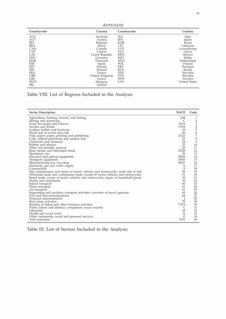
of the basic data. The dataset covers 40 regions (27 EU countries and 13 other majorcountries), which together account for approximately 85 % of world’s GDP in 2006.The WIOD data is disaggregated in 35 industries and provides detailed informationon primary (raw materials), secondary (manufacturing) as well as tertiary (services)sectors. In addition, it offers annual data which ranges from 1995 to 2006 and in partsto 2009. Beside its broad country coverage, detailed sectoral disaggregation and timeperiod character, the dataset has another important feature: it covers various aspectsof economic activity and for example involves accounts for energy and environmentalissues or socioeconomic and bilateral trade data. Employing the WIOD dataset inour estimation process involves three main benefits. We can estimate substitutionelasticities using one consistent dataset and do not have to merge potentially incom-patible data. The comprehensive sectoral coverage of WIOD allows us to estimatesubstitution elasticities for a broad set of sectors. Last but not least, for the firsttime we can derive elasticities from the same data which researchers can use also tocalibrate their simulations.In our analysis, we use in particular the WIOD Socio-Economic Accounts (SEA files)and the WIOD Energy Use tables (EU files). Taken together, they form a balancedpanel covering 40 regions and 35 sectors over a period of 12 years (1995 to 2006) andinclude detailed information on production in- and outputs. More specifically WIODsupplies us with data regarding the number of employees for the variable labourL, gross value added at basic prices for the variable value added VA, intermediateinputs at purchasers’ prices for the variable materials M, gross energy use for thevariable energy E and gross output at basic prices for the variable output Y. ButWIOD does not include the capital stock information required four our estimation.Generally, the Achilles’ heel of any empirical investigation of capital and laboursubstitutability is the capital stock variable. That is because it is usually hard toobtain reliable (physical) capital stock data from official sources, especially whenrequiring the data for a comprehensive set of regions and sectors. Unfortunately, tothis regard WIOD is no exception. However, WIOD nevertheless offers a solution tocircumvent this problem. It supplies quantity indices for physical capital stocks andinformation on gross fixed capital formation for each country, sector and year. We usethis information in order to construct our own capital stock data using the perpetualinventory method (e.g. Caselli , 2005).3 We are fully aware of the problem that theconstruction of own capital stock data and using it subsequently in our analysis isnot the first best solution. Therefore we check very carefully the consistency androbustness of the capital stock data we construct and compare our estimates withthe capital stock data provided in the Extended Penn World Tables 3.0 (Marquettiand Foley , 2008). The correlation of our estimate with the data from the EPWT 3.0is 0.9235. Hence we are convinced that our estimated values are sufficiently reliable.For the estimation, all monetary values have been transformed to U.S. Dollars using

3 At large, the perpetual inventory method consists of two steps. First, one estimates the initial capital stockK0 =

I0(g−δ)

, where I0 is the value of the investment series (in our case gross fixed capital formation in thefirst year (e.g. 1995 for many countries), g is the average geometric growth rate for the investment series,and δ the depreciation rate. We arbitrarily set the denominator to (g− δ) = 0.05 = 5%, although differentvalues will not affect the outcome significantly (Caselli , 2005). Next one applies a modified version of theperpetual equation Kt = It + Kt−1 · (1− δ) by using the sectoral and regional quantity indices in order tofinally construct the capital stocks.

6

the Penn World Table (Heston et al. , 2011) and are reported at 1995 prices. Energy isin Terajouls. Labour is given in thousand persons. Table I gives an overview of thevariables used in the estimation process. A complete list of the regions and sectorscovered by this analysis is given in the Appendix.

Variable Definition Source Unit

Output Gross output at basic prices WIOD SEA Files million 1995 USDCapital Capital stock Derived using WIOD SEA Files million 1995 USDLabour Number of employees WIOD SEA Files thousand personsValue Added Gross value added at basic prices WIOD SEA Files million 1995 USDEnergy Gross energy use WIOD EU Files TerajoulsMaterials Gross output at basic prices WIOD SEA Files million 1995 USD

Table I: Choice of Instruments

B. Estimation Procedure

CES functions are non-linear in parameters and hence parameters can initially notbe estimated using standard non-linear estimation techniques. For this reason anddue to the so far rather tricky implementation of non-linear estimation procedures,most researchers estimating elasticities of substitution within a CES framework workwith CES functions that have been linearised in some form or the other. Thereby, theso-called Kmenta approximation (Kmenta , 1967) has been very popular. However,the original CES function cannot be linarised analytically and using approximationmethods to linearise the CES function can have drawbacks. Kmenta (1967) himselfnotes that if in the production function under investigation the input ratio as wellas the elasticity of substitution are either very high or very low, his approximationmethod may not perform well. Maddala and Kadane (1967) and Thursby and Lovell(1978) confirm this problem and shows that the standard Kmenta procedure may notlead to reliable estimates of parameters in a CES framework.To avoid issues related to Kmenta approximations without having to use cumbersomenon-linear estimation procedures, researchers also make use from the cost functionapproach (e.g. van der Werf , 2008; Okagawa and Ban , 2008). Thereby one can takeadvantage of the cost function associated with a specific production function and de-rive a linear system of equations from the corresponding optimal input demand. Thiscan subsequently be used be used to estimate the function coefficients in question.But this approach requires comprehensive price data, which in most cases is ratherdifficult to come by, especially when undertaking sector specific analysis.In contrast to the majority of other studies investigating the substitutability of inputswithin a CES production structure, we estimate substitution elasticities directly fromthe CES production function and primarily building non-linear least-squares esti-mation procedures. Thereby we employ a set of different optimisation algorithms,namely the Levenberg-Marquardt algorithm (LM) (Marquardt , 1963), PORT routines(Gay , 1990), the Differential Evolution algorithm (DE) (Storn and Price , 1997; Priceet al. , 2005), Nelder-Mead routines (NM) (Nelder and Mead , 1965), the SimulatedAnnealing algorithm (SANN) (Kirkpatrick et al. , 1987; Cerny , 1985) and the socalled BFGS algorithm (Broyden , 1970; Fletcher , 1970; Goldfarb , 1970; Shanno ,

7

1970). In some estimation runs we make use of starting values compiled by means ofa preceding grid search for the substitution parameter ρ involving LM.4 A detailedoverview of all the estimations we run is given in Table X in the Appendix. However,after having shown that except for SANN and DE our results are robust with regardto the choice of the employed optimisation algorithm, we continue our analysis onthe basis of the estimation process producing the best fit to the our data. Id estestimations relying on LM and PORT with starting values.For the actual estimation process we use the programming environment R withthe package micEconCES developed by Henningsen and Henningsen (2011). Butthe micEconCES package in its current version only allows to estimate parametersfor a two-level nested CES production function. Yet we would like to derive thesubstitution elasticities for a three-level nested CES function. To overcome this lim-itation, we benefit from the separability implied by the CES framework and splitthe originally three-level nested KLEM CES function we would like to investigategiven by Equation (5) into two individual CES functions. Accordingly we estimatethe substitution elasticities first for the non-nested CES function

VAt = γKLetλ(

αKL(Kt)−ρKL + (1− αKL) (Lt)

−ρKL) 1−ρKL , (7)

with the substitution elasticity σKL = 11+ρKL

. Subsequently we do the same for thetwo-level CES function

Yt = γKLEMetλ (αKLEM(Mt)−ρKLEM + (1− αKLEM)

((αKLE(Et)

−ρKLE+

(1− αKLE) (VAt)−ρKLE

) 1−ρKLE

)−ρKLEM) 1−ρKLEM

,(8)

with the substitution elasticities σKLE = 11+ρKLE

and σKLEM = 11+ρKLEM

. Taken together,Equation (7) and Equation (8) represent the overall CES function in question, whereas,as already indicated by Equation (5), Equation (7) is the bottom nest and Equation(8) corresponds to the middle and upper nests of the production function underinvestigation.The substitution elasticities are estimated specifically for each of the 35 sectors avail-able in the WIOD dataset. Thereby, we pool all sectoral data across all regions. Asindicated by Equation (7) and (8), initially we assume that elasticities are constantover time. Hence, in our setting technological progress can only take place throughchanges in overall productivity. Though, this assumption is relaxed at a later stage.5

4 For more information on how adequate starting values are derived applying a preceding grid search, theinterested reader is kindly referred to Henningsen and Henningsen (2011).

5 It is also planned to relax the implicit assumption we have made by pooling all regions, i.e. that substitutionelasticities are equal across all regions, in a later version of this paper.

8

IV. ESTIMATION RESULTS

Unsurprisingly the estimates for the substitution parameters ρKL, ρKLE and ρKLEMand hence for σKL, σKLE and σKLEMdiffer across different estimation methods. Butall in all and in view of the respective standard errors, deviations are rather minor.Nevertheless we observe a small divergence between gradient-based local opimi-sation algorithms (BFGS, LM and PORT) and algorithms targeting global minima(e.g. NM). Robustness across estimation techniques decreases for smaller estimatedvalues of ρKL, ρKLE and ρKLEM and increases when adequate starting values from aprior grid search are used in the estimation process. The SANN and DE techniquehowever are exceptions and lead to notable different results in several cases, mainlysuggesting smaller values for ρKL, ρKLE and ρKLEM than other methods. Convergenceis tends also to be ann issue when applying these solvers. Given the overall robustnessof the different estimations, we choose to continue our analysis on the basis ofonly one estimation process. Evaluated on the basis of R-squared, the estimationsrelying on PORT routines and to a slightly smaller extent those using the LM andBFGS methodologies perform best. Without starting values from a preceding gridsearch, SANN generates the poorest fit. When using starting values, DE appearsto be the least powerful method. Furthermore, by the same measure, estimationsusing starting values from a preceding grid search generally have a better fit thanestimations without. This holds true for the investigation of Equation 7 as well asfor Equation 8. Given the benefit of the usage of starting values and on the wholevery similar estimation results, in the following we focus on the estimations withthe best fit to the data, id est estimations relying on PORT routines and which usestarting values. The corresponding estimation results for the substitution parameterρ are summarised in Table II. Note that for the middle and top nest of sector 5 wedo not achieve convergence for any acceptable convergence criteria. For this reasonthe respective estimates are put in brackets and we do not report the correspondingstandard deviation. Moreover, for sector 20 ρKL < 1 and hence violates the basicassumptions of the standard CES framework which requires σ ≥ 0 respectivelyρ ≥ −1. While so far we have applied an unrestricted estimation approach, thisindicates the need to incorporate the three parameter constraints implied by the CESframework γ > 0, 0 ≥ α ≥ 1 and σ ≥ 0 into our estimations.Table III summarises the results for ρ when applying the restricted estimation. Thecorresponding results for σ are given in Table XI in the Appendix. For obvious reasonsthe fit for the restricted model is not as good as before. Also the fact that for someestimates standard errors are disproportionate, in particular for such sectors in whichthe CES side constraints now incorporated in the estimation appear to be binding,indicates that the restricted estimation only provides a poor fit for some estimationstructures. However, as for the big majority of sectors and nests our estimation resultsseem to be reliable and as the usage of of CES functions has proven to be very popularin particular in CGE models, we proceed with our estimation process and continueincluding the constraints on γ, α and σ.Next we investigate whether the common simplification of using Cobb-Douglas orLeontief functions in CGE models can be rejected by our estimation results. Table IVpresents our findings to this regard.

9

Sector N ρKL-Est. Std. Dev. ρKLE-Est. Std. Dev. ρKLEM-Est. Std. Dev.

1 312 1.6574 0.2171 10.8130 75.7547 -0.1203 0.22092 372 -0.2188 0.1583 -0.0653 0.3649 3.5476 0.92813 396 3.1117 1.5527 3.1388 3.1956 -0.2518 0.19544 386 1.4786 0.3157 9.2629 31.2252 0.6197 0.12575 366 1.6643 0.6634 (-0.5546) (-0.3927)6 394 3.2492 1.3513 0.5652 0.3250 0.5715 0.35337 396 3.5233 1.8517 0.4236 0.1574 0.3953 0.31278 337 2.3792 2.0202 -0.8347 0.7198 2.2180 0.43949 396 0.9589 0.3316 -0.1870 0.2446 0.3105 0.426310 390 3.3969 0.9186 1.0095 0.5815 0.7903 0.573711 396 3.2845 0.7915 1.9604 15.5046 0.5797 0.296212 396 2.7039 0.6915 1.8853 12.3101 4.8660 0.845513 396 0.2231 0.0941 1.2727 0.6970 0.4808 0.215914 389 2.7392 3.3729 -0.0769 0.0892 0.1532 0.071015 378 0.7306 0.2182 1.9326 0.3736 0.6558 0.305016 380 0.6927 0.0874 0.3499 2.4342 0.8877 0.226617 393 2.4729 0.4808 2.3294 0.5525 -0.1704 0.107418 392 2.2705 0.5488 -0.1752 0.3118 0.3909 0.353619 394 3.5020 4.9176 1.2664 0.9783 0.3510 0.158820 396 -1.0961 0.1880 2.7734 0.6418 0.2937 0.121421 388 4.1859 1.2322 0.0006 0.5003 0.1705 0.096122 369 0.7799 0.1680 -0.0629 0.1491 -0.0250 0.080523 369 0.1533 0.1894 3.2972 1.4051 0.0127 0.308224 357 2.3662 1.5474 -0.1319 0.0979 0.0834 0.177425 333 0.2148 0.1828 10.0938 85.3278 -0.6582 0.063426 380 1.9993 0.7192 0.4409 0.2469 0.4031 0.049927 393 -0.6836 0.1271 0.3861 0.2780 -0.0998 0.419128 396 -0.1468 1.2603 1.8526 0.1484 -0.1149 0.153629 395 1.6551 0.3485 3.3117 0.3129 -0.2091 0.061630 392 2.2470 0.2941 -0.5723 0.4418 0.4738 0.180031 382 2.2569 0.4637 2.2032 0.3677 0.1004 0.114132 348 0.3012 0.2169 1.8523 0.6869 -0.3570 0.060733 377 1.3003 0.1534 0.0351 0.3132 -0.1804 0.051134 379 3.4606 0.8897 1.1655 3.8947 0.0993 0.306736 396 2.3914 0.4256 1.1437 0.9563 -0.1319 0.3495

Table II: Estimation Results for ρ (Unrestricted PORT Routine with Starting Values)

Sector N ρKL-Est. Std. Dev. ρKLE-Est. Std. Dev. ρKLEM-Est. Std. Dev.

1 312 1.9298 0.2978 -0.8088 0.9315 0.2795 0.24842 372 -0.2188 0.1583 (0.8531) >10 2.7609 0.76423 396 2.8095 1.4562 9.4384 7.2847 0.6105 0.18714 386 1.4056 0.3035 7.2389 4.1483 0.5954 0.12535 366 1.6772 0.6669 4.8139 2.1139 1.2755 0.13736 394 3.5327 1.5375 0.5652 0.3250 0.5715 0.35337 396 3.4305 1.7580 (1.7828) >10 0.4749 0.45418 337 2.2196 1.9217 -0.8727 0.5669 2.2518 0.44929 396 0.9419 0.3288 -0.1297 0.2485 0.3066 0.429810 390 3.4475 0.9363 (4.7844) >10 0.7958 0.568411 396 2.4896 0.5306 (0.1507) >10 0.5555 0.285312 396 2.2881 0.6016 (6.1628) >10 5.2304 0.973313 396 0.2231 0.0941 (-1.0000) >10 0.2674 0.192614 389 2.4643 3.0854 2.4279 1.3171 (-1.0000) 5.566615 378 0.7100 0.2133 2.0989 0.3833 0.8870 0.307416 380 0.6959 0.0877 -0.2106 1.7929 0.8503 0.224117 393 2.3098 0.4449 2.6268 0.5932 -0.1639 0.107218 392 2.2601 0.5455 (16.8981) >10 0.4158 0.369919 394 4.0696 6.6469 (3.8731) >10 0.4687 0.150920 396 (-1.0000) 0.1608 2.6537 0.5869 0.1992 0.120521 388 3.4819 0.9534 0.0457 0.4964 0.1517 0.096122 369 0.7606 0.1655 -0.0874 0.1585 0.2134 0.097023 369 0.1533 0.1894 3.4865 1.3732 0.0883 0.310324 357 2.3490 1.5388 -0.1663 0.0969 0.1943 0.179425 333 0.2155 0.1828 2.6182 1.9587 0.0289 0.093326 380 (1.7505) >10 0.4313 0.2419 0.4110 0.050527 393 -0.6323 0.1289 (33.9831) >10 -0.1487 0.382828 396 -0.2431 >10 1.8621 0.1505 -0.0335 0.157129 395 1.5531 0.3350 3.0418 0.2863 -0.2492 0.060430 392 2.1703 0.2795 (-0.1913) >10 0.5218 0.192531 382 2.8469 0.6145 (12.9564) >10 -0.1097 0.112632 348 (0.2123) >10 (-1.0000) 0.3746 -0.1290 0.077833 377 1.3197 0.1556 0.0726 0.3500 0.0302 0.057834 379 3.7657 1.0627 2.1341 3.3036 0.1336 0.307136 396 3.0092 0.5861 1.1437 0.9563 -0.1319 0.3495

Table III: Estimation Results for ρ (Restricted PORT Routine with Starting Values)

10

Sector H0: σKL = 0 H0: σKL = 1 H0: σKLE = 0 H0: σKLE = 1 H0: σKLEM = 0 H0: σKLEM = 11 <0.01 <0.01 <0.01 <0.01 <0.01 <0.012 <0.01 <0.01 <0.01 <0.013 <0.01 <0.01 <0.01 <0.01 <0.01 <0.014 <0.01 <0.01 <0.01 <0.01 <0.01 <0.015 <0.01 <0.01 <0.01 <0.01 <0.01 <0.016 <0.01 <0.01 <0.01 <0.01 <0.01 <0.017 <0.01 <0.01 <0.01 <0.018 <0.01 <0.01 <0.01 <0.01 <0.01 <0.019 <0.01 <0.01 <0.01 <0.01 <0.01 <0.0110 <0.01 <0.01 <0.01 <0.0111 <0.01 <0.01 <0.01 <0.0112 <0.01 <0.01 <0.01 <0.0113 <0.01 <0.01 <0.01 <0.01 <0.0114 <0.01 <0.01 <0.01 <0.01 <0.0115 <0.01 <0.01 <0.01 <0.01 <0.01 <0.0116 <0.01 <0.01 <0.01 <0.01 <0.0117 <0.01 <0.01 <0.01 <0.01 <0.01 <0.0118 <0.01 <0.01 <0.01 <0.01 <0.01 <0.0119 <0.01 <0.01 <0.01 <0.0120 <0.01 <0.01 <0.01 <0.01 <0.01 <0.0121 <0.01 <0.01 <0.01 <0.01 <0.0122 <0.01 <0.01 <0.01 <0.01 <0.01 <0.0123 <0.01 <0.01 <0.01 <0.01 <0.01 <0.0124 <0.01 <0.01 <0.01 <0.01 <0.01 <0.0125 <0.01 <0.01 <0.01 <0.01 <0.01 <0.0126 <0.01 <0.01 <0.01 <0.0127 <0.01 <0.01 <0.01 <0.0128 <0.01 <0.01 <0.01 <0.0129 <0.01 <0.01 <0.01 <0.01 <0.01 <0.0130 <0.01 <0.01 <0.01 <0.0131 <0.01 <0.01 <0.01 <0.01 <0.01 <0.0132 <0.01 <0.01 <0.01 <0.0133 <0.01 <0.01 <0.01 <0.01 <0.01 <0.0134 <0.01 <0.01 <0.01 <0.01 <0.01 <0.0136 <0.01 <0.01 <0.01 <0.01 <0.01 <0.01

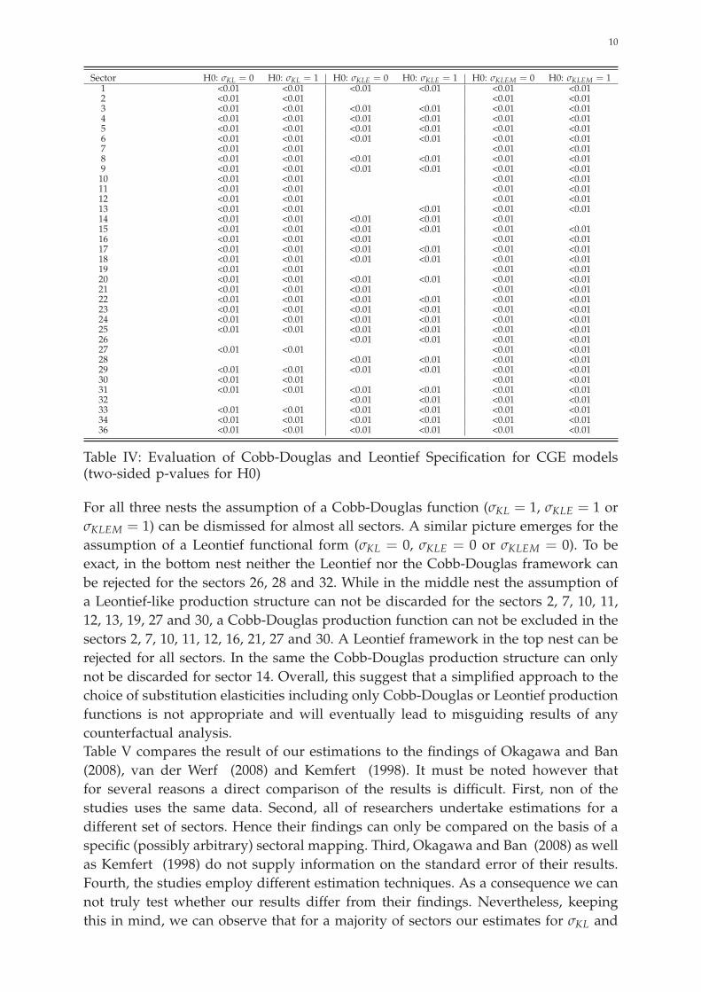
Table IV: Evaluation of Cobb-Douglas and Leontief Specification for CGE models(two-sided p-values for H0)

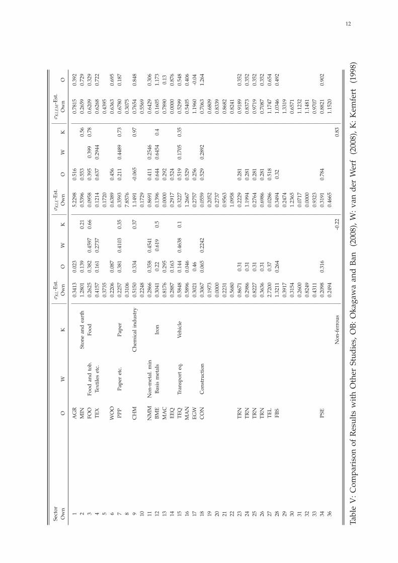
For all three nests the assumption of a Cobb-Douglas function (σKL = 1, σKLE = 1 orσKLEM = 1) can be dismissed for almost all sectors. A similar picture emerges for theassumption of a Leontief functional form (σKL = 0, σKLE = 0 or σKLEM = 0). To beexact, in the bottom nest neither the Leontief nor the Cobb-Douglas framework canbe rejected for the sectors 26, 28 and 32. While in the middle nest the assumption ofa Leontief-like production structure can not be discarded for the sectors 2, 7, 10, 11,12, 13, 19, 27 and 30, a Cobb-Douglas production function can not be excluded in thesectors 2, 7, 10, 11, 12, 16, 21, 27 and 30. A Leontief framework in the top nest can berejected for all sectors. In the same the Cobb-Douglas production structure can onlynot be discarded for sector 14. Overall, this suggest that a simplified approach to thechoice of substitution elasticities including only Cobb-Douglas or Leontief productionfunctions is not appropriate and will eventually lead to misguiding results of anycounterfactual analysis.Table V compares the result of our estimations to the findings of Okagawa and Ban(2008), van der Werf (2008) and Kemfert (1998). It must be noted however thatfor several reasons a direct comparison of the results is difficult. First, non of thestudies uses the same data. Second, all of researchers undertake estimations for adifferent set of sectors. Hence their findings can only be compared on the basis of aspecific (possibly arbitrary) sectoral mapping. Third, Okagawa and Ban (2008) as wellas Kemfert (1998) do not supply information on the standard error of their results.Fourth, the studies employ different estimation techniques. As a consequence we cannot truly test whether our results differ from their findings. Nevertheless, keepingthis in mind, we can observe that for a majority of sectors our estimates for σKL and

11

σKLEM tend to be higher than the substitution elasticities supplied by Okagawa andBan , although this does not hold true for our estimate of σKLE. Compared to theelasticities derived by van der Werf (2008) or Kemfert (1998), our estimates seemnot to be systematically smaller or bigger.Besides the more fundamental issues mentioned above, there are potentially severalreasons for the differences between our estimates and those from other studies.Our data may not be up to the task or our choice of instruments as illustrated inI is inappropriate. However, as Okagawa and Ban (2008), van der Werf (2008)as well as Kemfert (1998) use similar data and instruments, these issues do notimmediately suggest themselves as the main reasons for the deviations. Alternatively,the differences may arise due to the usage of different estimation approaches, inparticular with regard to linear or and non-linear estimation techniques. In effect,while Okagawa and Ban (2008), van der Werf (2008) and Kemfert (1998) estimatesubstitution elasticities using a linear estimation process, the elasticities derived inthis paper stem from a non-linear estimation process using the original functionalform of a CES production function.

12

Sector

σK

L-Est.

σK

LE-Est.

σK

LEM-Est.

Own

OW

KOwn

OW

KOwn

OW

KOwn

O

1AGR

0.3413

0.023

5.2298

0.516

0.7815

0.392

2MIN

Ston

eandearth

1.2801

0.139

0.21

0.5396

0.553

0.56

0.2659

0.729

3FO

OFo

odandtob.

Food

0.2625

0.382

0.4597

0.66

0.0958

0.395

0.399

0.78

0.6209

0.329

4TE

XTextilesetc.

0.4157

0.161

0.2737

0.1214

0.637

0.2944

0.6268

0.722

50.3735

0.1720

0.4395

6WOO

0.2206

0.087

0.6389

0.456

0.6363

0.695

7PP

PPa

peretc.

Paper

0.2257

0.381

0.4103

0.35

0.3593

0.211

0.4489

0.73

0.6780

0.187

80.3106

7.8576

0.3075

9CHM

Chemical

indu

stry

0.5150

0.334

0.37

1.1491

-0.065

0.97

0.7654

0.848

100.2248

0.1729

0.5569

11NMM

Non

-metal.m

in0.2866

0.358

0.4541

0.8691

0.411

0.2546

0.6429

0.306

12BM

EBa

sismetals

Iron

0.3041

0.22

0.619

0.5

0.1396

0.644

0.6454

0.4

0.1605

1.173

13MAC

0.8176

0.295

0.0000

0.292

0.7890

0.13

14EE

Q0.2887

0.163

0.2917

0.524

0.0000

0.876

15TE

QTransporteq.

Vehicle

0.5848

0.144

0.4638

0.1

0.3227

0.519

0.1705

0.35

0.5299

0.548

16MAN

0.5896

0.046

1.2667

0.529

0.5405

0.406

17EG

W0.3021

0.46

0.2757

0.256

1.1960

-0.04

18CON

Con

struction

0.3067

0.065

0.2242

0.0559

0.529

0.2892

0.7063

1.264

190.1973

0.2052

0.6809

200.0000

0.2737

0.8339

210.2231

0.9563

0.8682

220.5680

1.0958

0.8241

23TR

N0.8671

0.31

0.2229

0.281

0.9189

0.352

24TR

N0.2986

0.31

1.1994

0.281

0.8373

0.352

25TR

N0.8227

0.31

0.2764

0.281

0.9719

0.352

26TR

N0.3636

0.31

0.6986

0.281

0.7087

0.352

27TE

L2.7200

0.37

0.0286

0.518

1.1747

0.654

28FB

S1.3211

0.264

0.3494

0.32

1.0346

0.492

290.3917

0.2474

1.3319

300.3154

1.2365

0.6571

310.2600

0.0717

1.1232

320.8249

0.0000

1.1481

330.4311

0.9323

0.9707

34PS

E0.2098

0.316

0.3191

0.784

0.8821

0.902

360.2494

0.4665

1.1520

Non

-ferrous

-0.22

0.83

TableV:C

ompa

risonof

Results

withOther

Stud

ies,OB:

OkagawaandBa

n(2008),W

:van

derWerf(2008),K

:Kem

fert

(1998)

13

To test whether in our setting a linear estimation approach would yield differentresults, we once more estimate the substitution elasticities for σKL. But this time use astandard linear least-squares estimation process by applying Kmenta approximationsto Equation 7. Subsequently we contrast the results of this estimation with the resultsof a non-linear estimation process. For the non-linear estimation process we focus onan application using unrestricted LM algorithms and PORT routines with startingvalues from a preceding grid search, as these methods have proven to be robustand advantageous with regard to low values of sum of squared residuals. However,in contrast to the previous estimation exercises in this paper, this time we do notaccount for technological change because the Henningsen and Henningsen (2011)implementation of the Kmenta methodology does currently not support this andhence the findings of the estimations would else not be comparable.

Kmenta LM-nTP PORT-nTPSector ρKL-Est. Std. Dev. r2 ρKL-Est. Std. Dev. r2 ρKL-Est. Std. Dev. r2

1 -0.0975 0.0512 0.7188 2.5709 0.6335 0.9301 2.7753 0.7486 0.93022 0.1479 0.1551 0.7483 -0.3388 0.1583 0.7790 -0.3388 0.1583 0.77903 -0.2328 0.0942 0.7781 2.9479 1.4164 0.9393 5.8768 2.6447 0.94274 -0.1101 0.0838 0.9076 1.1809 0.2534 0.9375 1.1809 0.2534 0.93755 (-1.2913) 0.9627 -6.8546 2.0952 0.7796 0.8566 2.0957 0.7798 0.85666 -0.3295 0.0542 -0.7801 3.5345 1.5014 0.8758 3.7635 1.6540 0.87587 -0.4825 0.1944 -1.7921 3.5692 1.7306 0.9516 5.3638 3.5857 0.95228 0.2591 0.1383 0.1066 1.9984 2.0939 0.7362 3.8117 3.3731 0.74059 -0.4286 0.1236 0.8955 0.5048 0.3207 0.9782 0.5049 0.3207 0.978210 -0.5023 0.2860 0.9298 3.2378 0.8941 0.9682 5.2990 1.5307 0.968611 -0.2415 0.1018 0.7893 3.2151 0.7777 0.9348 5.3529 1.7959 0.936612 -0.4881 0.1863 -0.4663 3.1623 0.8161 0.9633 3.6084 0.9377 0.963313 -0.0288 0.1188 0.8369 0.1247 0.0886 0.9439 0.1247 0.0886 0.943914 -0.3954 0.1159 0.2269 (-24.5419) >10 0.4876 (-0.4290) >10 0.487615 0.7852 1.4001 0.1832 2.8643 0.9524 0.9673 4.5096 1.3205 0.967616 (-2.7733) 6.5722 -2.8190 0.6971 0.0985 0.9708 0.6971 0.0985 0.970817 0.0885 0.6150 0.8815 2.3392 0.4698 0.9643 4.3153 0.9222 0.968618 -0.2422 0.0324 -2.9987 3.7564 1.0406 0.9755 5.7376 1.8229 0.975619 -0.3754 0.1876 0.7667 -0.6303 0.3866 0.8442 -0.6304 0.3867 0.844220 2.8902 3.9597 -0.0362 (-1.5664) 0.2828 0.9872 -1.0000 0.1166 0.986921 -0.0840 0.1610 0.7598 4.2021 1.2766 0.9709 6.6483 2.3976 0.973122 -0.2815 0.0464 -0.2446 0.8019 0.1730 0.9882 0.8019 0.1730 0.988223 -0.5170 0.2903 -1.8622 0.0890 0.1813 0.8931 0.0890 0.1813 0.893124 0.4366 0.4751 0.4011 2.2233 1.3725 0.7364 4.2390 5.5695 0.739725 -0.2693 0.2378 0.9189 0.7668 0.4022 0.9524 0.7674 0.4024 0.952426 -0.1807 0.0194 -8.4357 1.5332 0.6465 0.9295 (1.4075) >10 0.915027 -0.3549 0.1531 0.9488 (-1.0177) 0.1902 0.9758 (-1.0000) 0.1886 0.975828 0.2161 0.0563 0.2677 -0.4158 0.8492 0.9723 (-0.2856) >10 0.971129 -0.2285 0.0869 0.9718 1.9512 0.4056 0.9803 2.9891 0.6782 0.981030 0.0803 0.1089 0.8420 2.5427 0.3550 0.9889 2.5425 0.3549 0.988931 0.1379 0.2258 0.7453 3.1363 0.5745 0.9742 5.7789 1.3288 0.975832 1.1659 0.9564 0.0575 0.3664 0.2205 0.5195 (0.1538) >10 0.177233 -0.3098 0.0349 -5.4857 1.4023 0.1715 0.9905 1.4022 0.1715 0.990534 -0.5547 0.1587 0.3724 3.1975 0.7226 0.9696 3.4592 0.8509 0.969736 -0.1341 0.0780 0.9120 3.0612 0.6883 0.9836 5.3392 1.1823 0.9847

Table VI: Comparison Standard Linear Estimation and Non-Linear Estimation

Table VI summaries the results of the three estimations and contrasts their findings.Apart of few exceptions, estimates for ρKL using the non-linear estimation tech-niques are higher than those relying on the standard linear estimation approachusing Kmenta approximations. As noted in Section III, the usage of the Kmentaapproximation itself may lead to biased results, although it remains unclear whetherelasticities are over- or underestimated (Thursby and Lovell , 1978). In this contextthe former potentially seems to be the case. Furthermore, valued on the basis of themultiple R-squared, non-linear estimations perform clearly better than those relyingon standard linear procedures. In some cases of the Kmenta apporach R-squared is

14

even negative, indicating that using the simple average would perform better thanan estimation building on a Kmenta approximation of the CES function in question.According to our estimations, the Kmenta approach performs in particular bad incases where ρ is relatively low, respectively σ relatively high. This result is also inline with the observations of Thursby and Lovell (1978). Overall, the comparativelypoor performance of the non-linear estimation approach supports our preference withrespect to non-linear estimation procedures.The time series character of our data allows us to engage in an additional analysis andmakes it possible to investigate whether substitution elasticities change over time. Inthe economic literature, technological progress within the CES framework is mainlyunderstood as a change in input productivity and researchers focus primarily on de-termining λ in Equations 9 and 4. But in principle the CES framework for productionfunctions leaves room for technological change affecting not only productivity butalso the substitutability between different production inputs. In this case a modifiedCES function which takes into account changes of the substitution parameter overtime and incorporates Hicks-neutral technological change would take the form:

y = γeλt

(∑

iαi(xi)

−ρt

) 1−ρt

. (9)

The textile industry at the end of the 18th century provides an excellent exampleof this form of technological change. As looms became more and more advanced,human labour could be replaced more easily in the production process. Eventuallythis had a huge effect on business and society in that period.Embarking on a simple approach, we test whether we can observe a change in inputsubstitutability over time by reestimating and comparing σ for two different timeperiods (1995 to 1997 and 2004 to 2006). Table VII summarises the results to thisregard. In the bottom and middle nest, the hypothesis that the substitution elasticitiesdo not change over time can be rejected for about a third of the sectors underinvestigation. The inverse holds true for the the top nest and a significant change inthe substitutability between materials and the labour-capital-energy composite canbe observed for two thirds of the sectors. Hence, although significantly changingsubstitution elasticities appear not to be a problem for the majority of our estimations,the issue is potentially important. As a consequence, in future research this particulardimension of technological progress needs be taken into account and should beinvestigated with more rigour. Ultimately this will require studying longer timeperiods as those under investigation so far in studies on the substitutability of inputsand also a formalisation of the issue within the CES framework.

15

Sector

H0:

σK

L 95−

97=

σK

L 04−

06H0:|σ K

L 95−

97−

σK

L 04−

06|>

1H0:

σK

LE95−9

7=

σK

LE04−0

6H0:

|σ

KLE

95−9

7−

σK

LE04−0

6|>

1H0:

σK

LEM

95−9

7=

σK

LEM

04−0

6H0:

|σ

KLE

M95−9

7−

σK

LEM

04−0

6|>

11

<0.01

<0.01

<0.01

2<0

.05

<0.01

<0.01

3<0

.01

<0.01

<0.01

4<0

.01

<0.01

<0.01

<0.01

<0.01

5<0

.1<0

.01

<0.01

<0.01

6<0

.01

<0.01

<0.01

<0.01

7<0

.01

<0.05

<0.01

8<0

.01

<0.01

<0.01

<0.01

9<0

.01

<0.01

<0.01

<0.01

<0.01

10<0

.01

<0.01

11<0

.01

<0.01

<0.01

12<0

.01

<0.01

<0.01

<0.01

13<0

.01

<0.01

<0.01

<0.01

14<0

.01

<0.01

15<0

.1<0

.01

<0.01

<0.01

16<0

.01

<0.01

<0.01

17<0

.01

<0.01

18<0

.01

<0.01

<0.01

19<0

.01

<0.01

<0.01

20<0

.01

<0.01

<0.01

21<0

.1<0

.01

<0.01

22<0

.01

<0.01

<0.01

<0.01

<0.01

23<0

.01

<0.1

<0.01

24<0

.01

<0.01

<0.01

<0.01

<0.01

25<0

.01

<0.01

<0.01

<0.01

26<0

.01

<0.01

<0.01

27<0

.01

<0.01

<0.01

28<0

.01

<0.01

<0.01

<0.01

29<0

.01

<0.01

<0.01

30<0

.01

<0.01

<0.01

<0.01

31<0

.01

<0.01

<0.01

32<0

.01

33<0

.01

<0.01

<0.01

<0.01

<0.01

<0.01

34<0

.01

<0.05

<0.01

36<0

.01

<0.01

<0.01

<0.05

<0.01

<0.01

TableVII:C

ompa

risonof

theSu

bstitution

Elasticities

forthePeriod

s1995-1997and2004-2006(p-valuesforH0)

16

V. SUMMARY AND CONCLUSION

Elasticities, in particular substitution elasticities, are vital parameters for any micro-consistent economic model and crucially influence the results of counterfactual policyanalysis. But so far only few consistent estimates of elasticities exist. With this paperwe aim at overcoming this problem. Building on a rich dataset based on the WIODdata, we systematically estimate substitution elasticities for a comprehensive set ofsectors using different non-linear estimation procedures.Our results show that compared to standard linear estimations using Kmenta approx-imations, non-linear estimation techniques perform significantly better in this context.Moreover, no significant change in input substitutability takes place over during thetime period we consider. Hence for most sectors we do not observe technologicalchange through this channel. Although technological progress in the form of chang-ing substitution elasticities may potentially be an issue when studying longer timeperiods. On the basis of our estimations, we demonstrate that the common practiceof using Cobb-Douglas or Leontief production functions in economic models must berejected for the majority of sectors. As a consequence we object a simplified approachto the choice of substitution elasticities in the framework of policy oriented economicmodelling. In particular in response to this result, we provide a comprehensive setof consistently estimated substitution elasticities covering 35 sectors. Therewith wehope to make a valuable contribution to making instruments designed to evaluatepolicy measures ex-ante more reliable and support policy makers in their efforts tocope with global environmental problems such as climate change.

17

REFERENCES

ARROW, K.J., CHENERY, H.B., MINHAS, B.S. and SOLOW, R.M. (1961): Capital-LaborSubstitution and Economic Efficiency, in: The Review of Economics and Statistics,Vol. 43, pp. 225-250.

BALISTRERI, E.J., MCDANIEL, C.A., and WONG, E.V. (2003): n estimation of USindustry-level capital-labor substitution elasticities: Support for Cobb-Douglas, in:The North American Journal of Economics and Finance, Vol. 14, pp. 343-356.

BÖHRINGER, C., RUTHERFORD, T.F., and WIEGARD, W. (2003): Computable GeneralEquilibrium Analysis: Opening a Black Box, in: ZEW Discussion Paper, No. 03-56.

BROWNING, M., HANSEN, L.P., and HECKMAN, J. J. (1999): Micro data and generalequilibrium models, in: Handbook of Macroeconomics, Vol. 1, Part A, Chapter 8,pp. 543-633.

BROYDEN, C.G. (1970): The Convergence of a Class of Double-rank MinimizationAlgorithms, in: Journal of the Institute of Mathematics and Its Applications, Vol. 6,pp. 76-90.

CASELLI, F. (2005): Accounting for Cross-Country Income Differences, in: Handbookof Economic Growth, Vol. 1, No. 1, Chapter 9, pp. 679-741.

CERNY, V. (1985): Thermodynamical approach to the traveling salesman problem: Anefficient simulation algorithm, in: Journal of Optimization Theory and Applications,Vol. 45, pp. 41-51.

DAWKINS, C., SRINIVASAN, T.N., WHALLEY, J., and HECKMAN, J. J. (2001): Calibra-tion, in: Handbook of Econometrics, Vol. 5, Chapter 58, pp. 3653-3703.

DEVARAJAN, S. and ROBINSON, S. (2002): The influence of computable generalequilibrium models on policy, in: TMD Discussion Paper.

FLETCHER, R. (1970): A New Approach to Variable Metric Algorithms, in: ComputerJournal, Vol. 13, pp. 317-322.

GAY, D.M. (1990): Usage Summary for Selected Optimization Routines, in: AT & TBell Laboratories.

GOLDFARB, D.A. (1970): A Family of Variable Metric Updates Derived by VariationalMeans, in: Mathematics of Computation, Vol. 24, pp. 23-26.

HENNINGSEN, A. and HENNINGSEN, G. (2002): Econometric Estimation of theConstant Elasticity of Substitution Function in R: Package micEconCES, in: FOIWorking Paper, No. 9.

HESTON, Alan, Robert SUMMERS and Bettina ATEN (2011): Penn World TablesVersion 7.0, by: Center for International Comparisons of Production, Income andPrices at the University of Pennsylvania, 2011.

JACOBY, H.D., REILLY, J.M., MCFARLAND, J.R., and PALTSEV, S. (2006): Technologyand technical change in the MIT EPPA model, in: Energy Economics, Vol. 28, pp.610-631.

KEMFERT, C. (1998): Estimated substitution elasticities of a nested CES productionfunction approach for Germany, in: Energy Economics, Vol. 20, pp. 249-264.

KIRKPATRICK, S., GELATT, C.D.J.., and VECCHI (1987): Optimization by simulatedannealing Computer vision: issues, problems, principles, and paradigms, in: Com-puter Vision: Issues, Problems, Principles, and Paradigms, Chapter 5, pp. 606-615.

KLUMP, R. and DE LA GRANDVILLE, O. (2000): Economic Growth and the Elasticity

18

of Substitution, in: The American Economic Review, Vol. 90(1), pp. 282–91.KMENTA, J. (1967): On Estimation of the CES Production Function, in: International

Economic Review, Vol. 8, pp. 180-189.LEÓN-LEDESMA, M. A., MCADAM, P. and WILLMAN, A. (2010): Identifying theElasticity of Substitution with Biased Technical Change, in: The American EconomicReview, Vol. 100, pp. 1330-1357.

MADDALA, G.S. and KADANE, J.B. (1967): Estimation of Returns to Scale and theElasticity of Substitution, in: Econometrica, Vol. 35, pp. 419-423.

MARQUETTI, A. and FOLEY, D. (2008): Extended Penn World Tables Version 3.0,http://homepage.newschool.edu/˜foleyd/epwt/

MANSUR, A.H. and WHALLEY, J. (1984): Numerical Specification of Applied Gen-eral Equilibrium Models: Estimation, Calibration and Data, in: Applied GeneralEquilibrium Analysis.

MARQUARDT, D.W. (1963): An Algorithm for Least-Squares Estimations of NonlinearParameters, in: Journal of the Society for Industrial and Applied Mathematics, Vol.11, pp. 431-441.

MCKITRICK, R.R. (1998): The econometric critique of computable general equilibriummodeling: the role of functional forms, in: Economic Modelling, Vol. 15, pp. 543-573.

NELDER, J. and MEAD, R. (1965): A Simplex Method for Function Minimization, in:The Computer Journal, Vol. 7, pp. 308-313.

OKAGAWA, A. and BAN, K. (2008): Estimation of substitution elasticities for CGEmodels, in: Discussion Papers in Economics and Business, No. 08-16.

PRICE, K.V., STORN, R.M., and LAMPINEN, J.A. (2005): Differential evolution: apractical approach to global optimization, Springer, Heidelberg, Germany.

SALTER W.E.G. (1966): Productivity and Technical Change, 2nd edition (1st edition1960), Cambridge University Press, Cambridge, UK.

SATO, K. (1967): A Two-Level Constant-Elasticity-of-Substitution Production Func-tion, in: The Review of Economic Studies, Vol. 34, pp. 201-218.

SHANNO, D.F. (1970): Conditioning of Quasi-Newton Methods for Function Mini-mization, in: Mathematics of Computation, Vol. 24, pp. 647-656.

SOLOW, R. M. (1956): A Contribution to the Theory of Economic Growth, in: TheQuarterly Journal of Economics, Vol. 70, pp. 65-94.

STORN, R. and PRICE K. (1997): Differential Evolution - A Simple and EfficientHeuristic for global Optimization over Continuous Spaces, in: Journal of GlobalOptimization, Vol. 11, pp. 341-359.

SUE WING, I. (2004): Computable General Equilibrium Models and Their Use inEconomy-Wide Policy Analysis: Everything You Ever Wanted to Know (But WereAfraid to Ask), in: MIT Technical Note, No. 6.

THURSBY, J.G. and LOVELL C.A.K. (1978): An Investigation of the Kmenta Approxi-mation to the CES Function, in: International Economic Review, Vol. 19, pp. 363-377.

VAN DER WERF, E. (2008): Production functions for climate policy modeling: Anempirical analysis, in: Energy Economics, Vol. 30, pp. 2964-2979.

VON WEIZSÄCKER, C.C. (1966): Tentative Notes on a Two Sector Model with InducedTechnical Progress, in: The Review of Economic Studies, Vol. 33, pp. 245-251.

19

APPENDIX

Countrycode Country Countrycode Country

AUS Australia ITA ItalyAUT Austria JPN JapanBEL Belgium KOR KoreaBRA Brazil LTU LithuaniaCAN Canada LUX LuxembourgCYP Cyprus LVA LatviaCZE Czech Republic MEX MexicoDEU Germany MLT MaltaDNK Denmark NLD NetherlandsESP Spain POL PolandEST Estonia PRT PortugalFIN Finland RUS RussiaFRA France SVK SlovakiaGBR United Kingdom SVN SloveniaGRC Greece SWE SwedenHUN Hungary USA United StatesIRL Ireland

Table VIII: List of Regions Included in the Analysis

Sector Description NACE Code

Agriculture, hunting, forestry and fishing AtB 1Mining and quarrying C 2Food, beverages and tobacco 15t16 3Textiles and textile 17t18 4Leather, leather and footwear 19 5Wood and of wood and cork 20 6Pulp, paper, paper, printing and publishing 21t22 7Coke, refined petroleum and nuclear fuel 23 8Chemicals and chemical 24 9Rubber and plastics 25 10Other non-metallic mineral 26 11Basic metals and fabricated metal 27t28 12Machinery, nec 29 13Electrical and optical equipment 30t33 14Transport equipment 34t35 15Manufacturing nec; recycling 36t37 16Electricity, gas and water supply E 17Construction F 18Sale, maintenance and repair of motor vehicles and motorcycles; retail sale of fuel 50 19Wholesale trade and commission trade, except of motor vehicles and motorcycles 51 20Retail trade, except of motor vehicles and motorcycles; repair of household goods 52 21Hotels and restaurants H 22Inland transport 60 23Water transport 61 24Air transport 62 25Supporting and auxiliary transport activities; activities of travel agencies 63 26Post and telecommunications 64 27Financial intermediation J 28Real estate activities 70 29Renting of m&eq and other business activities 71t74 30Public admin and defence; compulsory social security L 31Education M 32Health and social work N 33Other community, social and personal services O 34Total industries TOT 36

Table IX: List of Sectors Included in the Analysis

20

Solver Starting Values Restricted Coefficients Technological Progressfrom Grid Search (γ ≥ 0, 0 ≤ αi ≤ 1,∑n

i=1 αi , ρ ≥ −1) (Hicks-neutral)BFGS no no yes

yes no yes

DE no no yesno yes yes

KM no no no

LM no no yesyes no yesno no noyes no no

NM no no yesyes no yes

PORT no no yesno yes yesyes no yesyes yes yesno no nono yes noyes no noyes yes no

SANN no no yesyes no yes

Table X: List of Estimations Procedures Included in the Analysis

Sector N σKL-Est. Std. Dev. σKLE-Est. Std. Dev. σKLEM-Est. Std. Dev.

1 312 0.3413 0.0347 (5.2298) >10 0.7815 0.15172 372 1.2801 0.2594 (0.5396) >10 0.2659 0.05403 396 0.2625 0.1003 0.0958 0.0669 0.6209 0.07224 386 0.4157 0.0525 0.1214 0.0611 0.6268 0.04925 366 0.3735 0.0930 0.1720 0.0625 0.4395 0.02656 394 0.2206 0.0748 0.6389 0.1327 0.6363 0.14317 396 0.2257 0.0896 (0.3593) >10 0.6780 0.20878 337 0.3106 0.1854 (7.8576) >10 0.3075 0.04259 396 0.5150 0.0872 1.1491 0.3281 0.7654 0.251710 390 0.2248 0.0473 (0.1729) >10 0.5569 0.176211 396 0.2866 0.0436 (0.8691) >10 0.6429 0.117912 396 0.3041 0.0556 (0.1396) >10 0.1605 0.025113 396 0.8176 0.0629 (0.0000) (0.0000) 0.7890 0.119914 389 0.2887 0.2571 0.2917 0.1121 (0.0000) (0.0000)15 378 0.5848 0.0729 0.3227 0.0399 0.5299 0.086316 380 0.5896 0.0305 1.2667 2.8770 0.5405 0.065517 393 0.3021 0.0406 0.2757 0.0451 1.1960 0.153318 392 0.3067 0.0513 0.0559 0.2692 0.7063 0.184619 394 0.1973 0.2586 (0.2052) >10 0.6809 0.070020 396 (0.0000) (0.0000) 0.2737 0.0440 0.8339 0.083821 388 0.2231 0.0475 0.9563 0.4540 0.8682 0.072422 369 0.5680 0.0534 1.0958 0.1904 0.8241 0.065923 369 0.8671 0.1424 0.2229 0.0682 0.9189 0.262024 357 0.2986 0.1372 1.1994 0.1394 0.8373 0.125825 333 0.8227 0.1237 0.2764 0.1496 0.9719 0.088126 380 (0.3636) >10 0.6986 0.1181 0.7087 0.025427 393 2.7200 0.9540 (0.0286) >10 1.1747 0.528328 396 (1.3211) >10 0.3494 0.0184 1.0346 0.168229 395 0.3917 0.0514 0.2474 0.0175 1.3319 0.107230 392 0.3154 0.0278 (1.2365) >10 0.6571 0.083131 382 0.2600 0.0415 0.0717 0.4378 1.1232 0.142132 348 (0.8249) >10 (0.0000) (0.0000) 1.1481 0.102533 377 0.4311 0.0289 0.9323 0.3042 0.9707 0.054534 379 0.2098 0.0468 0.3191 0.3363 0.8821 0.239036 396 0.2494 0.0365 0.4665 0.2081 1.1520 0.4638

Table XI: Estimation Results for σ (Restricted PORT Routine with Starting Values)