Substitutability and protectionism: Latin America’s trade...
33
Substitutability and protectionism: Latin America’s trade policy and imports from China and India* Giovanni Facchini†, Marcelo Olarreaga‡, Peri Silva§, Gerald Willmann¶ Abstract This paper examines the trade policy response of Latin American governments to the rapid growth of China and India in world markets. To explain higher protection in sectors where a large share is imported from these countries, we extend the ‘protection for sale’ model to allow for different degrees of substitutability between domestically produced and imported varieties. The extension suggests that higher levels of protection towards Chinese goods can be explained by high substitutability between domestically produced goods and Chinese goods, whereas lower levels of protection towards goods imported from India can be explained by low substitutability with domestically produced goods. The data support the extension to the ‘protection for sale’ model, which performs better than the original specification in terms of explaining Latin America’s structure of protection. JEL classification numbers: F10, F11, F13 Keywords: Latin America, Protectionism. World Bank Policy Research Working Paper 4188, April 2007 The Policy Research Working Paper Series disseminates the findings of work in progress to encourage the exchange of ideas about development issues. An objective of the series is to get the findings out quickly, even if the presentations are less than fully polished. The papers carry the names of the authors and should be cited accordingly. The findings, interpretations, and conclusions expressed in this paper are entirely those of the authors. They do not necessarily represent the view of the World Bank, its Executive Directors, or the countries they represent. Policy Research Working Papers are available online at http://econ.worldbank.org. *We are grateful to Pravin Krishna, and participants at seminars organized by the CEPR in Paris, the University of Nottingham, and the World Bank for constructive comments and suggestions on an earlier version. This project was supported by the World Bank’s Chief Economist Office for Latin America and the Research Support Budget. Peri Silva acknowledges financial support from the College of Business and Public Administration at the University of North Dakota. †Universit´a degli Studi di Milano, University of Illinois, Centro Studi Luca d’Agliano and CEPR. Email: [email protected]. ‡Office of the Chief Economist for Latin America, Banco Mundial, Carrera 7, no 7-21, Piso 16, Bogota, Colombia, and CEPR, London UK; phone: (571)326.3600 (ext. 257); fax: (571)326.3600; email: [email protected]. §University of North Dakota, Gamble 290 L. Centennial Drive, Grand Forks, ND 58202, USA; phone: (1.701)777-3351; email: [email protected]. ¶Christian-Albrechts-Unversitat zu Kiel, Wilhelm-Seelig-Platz 1, 24098 Kiel, Germany; phone: (49.431)880-3354; fax: (49.431)880-3150; email: [email protected]. WPS4188 Public Disclosure Authorized Public Disclosure Authorized Public Disclosure Authorized Public Disclosure Authorized Public Disclosure Authorized Public Disclosure Authorized Public Disclosure Authorized Public Disclosure Authorized
Transcript of Substitutability and protectionism: Latin America’s trade...
Substitutability and protectionism: Latin America’s trade policy and imports from
China and India*
Giovanni Facchini†, Marcelo Olarreaga‡, Peri Silva§, Gerald Willmann¶
Abstract This paper examines the trade policy response of Latin American governments to the rapid growth of China and India in world markets. To explain higher protection in sectors where a large share is imported from these countries, we extend the ‘protection for sale’ model to allow for different degrees of substitutability between domestically produced and imported varieties. The extension suggests that higher levels of protection towards Chinese goods can be explained by high substitutability between domestically produced goods and Chinese goods, whereas lower levels of protection towards goods imported from India can be explained by low substitutability with domestically produced goods. The data support the extension to the ‘protection for sale’ model, which performs better than the original specification in terms of explaining Latin America’s structure of protection. JEL classification numbers: F10, F11, F13 Keywords: Latin America, Protectionism.
World Bank Policy Research Working Paper 4188, April 2007 The Policy Research Working Paper Series disseminates the findings of work in progress to encourage the exchange of ideas about development issues. An objective of the series is to get the findings out quickly, even if the presentations are less than fully polished. The papers carry the names of the authors and should be cited accordingly. The findings, interpretations, and conclusions expressed in this paper are entirely those of the authors. They do not necessarily represent the view of the World Bank, its Executive Directors, or the countries they represent. Policy Research Working Papers are available online at http://econ.worldbank.org. *We are grateful to Pravin Krishna, and participants at seminars organized by the CEPR in Paris, the University of Nottingham, and the World Bank for constructive comments and suggestions on an earlier version. This project was supported by the World Bank’s Chief Economist Office for Latin America and the Research Support Budget. Peri Silva acknowledges financial support from the College of Business and Public Administration at the University of North Dakota. †Universit´a degli Studi di Milano, University of Illinois, Centro Studi Luca d’Agliano and CEPR. Email: [email protected]. ‡Office of the Chief Economist for Latin America, Banco Mundial, Carrera 7, no 7-21, Piso 16, Bogota, Colombia, and CEPR, London UK; phone: (571)326.3600 (ext. 257); fax: (571)326.3600; email: [email protected]. §University of North Dakota, Gamble 290 L. Centennial Drive, Grand Forks, ND 58202, USA; phone: (1.701)777-3351; email: [email protected]. ¶Christian-Albrechts-Unversitat zu Kiel, Wilhelm-Seelig-Platz 1, 24098 Kiel, Germany; phone: (49.431)880-3354; fax: (49.431)880-3150; email: [email protected].
WPS4188
Pub
lic D
iscl
osur
e A
utho
rized
Pub
lic D
iscl
osur
e A
utho
rized
Pub
lic D
iscl
osur
e A
utho
rized
Pub
lic D
iscl
osur
e A
utho
rized
Pub
lic D
iscl
osur
e A
utho
rized
Pub
lic D
iscl
osur
e A
utho
rized
Pub
lic D
iscl
osur
e A
utho
rized
Pub
lic D
iscl
osur
e A
utho
rized
1 Introduction
China’s and India’s fast economic growth during the past decade is paralleled by their in-
creased presence in policy discussions throughout Latin America. The success of the two
Asian economies is not only looked upon with admiration, but is often accompanied by
concerns about the effects that growing trade integration with China (and India to a lesser
extent) has on the manufacturing sector throughout the region. Textiles, apparel, shoe
manufacturing and toys are amongst the sectors worst hit by international competition.
In many Latin American countries requests for explicit protection are becoming more
and more common. At the end of 2005 as Brazilian imports of textiles from China surged,
Brazilian manufacturers officially asked their government to limit imports of Chinese silk,
velvet and polyester thread by imposing import quotas and/or increasing tariffs. At the time,
they also noted that an additional 70 Chinese products were being reviewed by the textile
industry to determine whether similar protective measures are to be requested. A comunique
by Argentina’s Confederation of Medium Enterprises (CAME) calls for not repeating the
“mistakes of the nineties, when an ‘invasion’ of Chinese products destroyed entire sectors of
the manufacturing sector.”1
Local politicians have not left these calls for help unanswered. After a recent meeting with
its Chinese counterpart, the Brazilian Minister for Industry, Development and Commerce
Luiz Furlan was quick to highlight that “I made it very clear to Minister Bo Xilai that we
will take the legal steps to give Brazilian industry the right to protect itself”.2 In early
2006, and following the earlier demands of Brazilian textile manufacturers, Brazil and China
signed an agreement under which China was to limit its export growth of 70 textile products
to Brazil. Notwithstanding their country’s privileged access to the US market, Mexican
politicians show similar feelings and are growing more and more nervous about Mexico’s
burgeoning trade deficit with China. It is not surprising then that after a recent meeting
with Chinese leaders, president Fox was very happy to report that “Today we heard from
1See CAME’s comunique of November 16th 2004 at http://procom.org.ar/comunicado.php3?id=335.2As reported by Yahoo! on October 4 2005. See http://sg.biz.yahoo.com/051004/1/3veny.htm.
1

President Hu his enthusiasm, his help, his support in closing the commercial gap...”.3
While GATT-WTO bounds in principle do not allow countries to increase protection vis
a vis China and India’s products, most developing countries have bound tariffs well above
their applied levels, a situation that de facto enables them to significantly increase protection
without violating their GATT obligations.4 Similarly, antidumping and safeguard rules are
quite lax and these instruments have been often used by both developed and developing
countries against Chinese imports (at least until China’s accession to the WTO).5
Given the substantial degree of flexibility enjoyed by domestic policy makers in imple-
menting trade policies within the WTO rules, we are interested in exploring whether the
characterization of China and India as sources of “cheap” and “unfair” imports has led to
increased protectionism on goods that are heavily imported from the two Asian economies.6
Our initial analysis indicates that this is indeed the case for Latin American imports
from China. Controlling for time, country, and industry fixed effects and instrumenting the
import share of China and India to account for potential reverse causality, we find that on
average, tariffs and non tariff barriers tend to be higher for goods that are heavily imported
from China. Goods imported from India, on the other hand, tend to face lower levels of
protection than imports from the rest of the world. Among Latin American regions, this
result holds for the Andean countries, the Southern Cone and Mexico, while in the case of
Central America there is evidence of lower levels of protection on goods imported from both
China and India.
Motivated by this first-pass empirical evidence, we turn to a more structural explanation
of the differences in the levels of protection observed in goods imported heavily from China
3See “Mexico builds trade ties with China” by J.C. McKinley in The New York Times of September 19,2005.
4For example, Brazil’s bound tariff in textiles, apparel and footwear are bound at 35% in the WTO, andapplied tariffs on these products have varied between 16 and 30 percent during the 1990s.
5See Hoekman and Kostecki (2001).6Below are some common characterizations of China as a source of “cheap” and “unfair” imports: “Coun-
tries around the world are bracing for a surge of cheap imports from China, which benefits from cheap,union-free labor and rising productivity” Taipei Times, January 2nd 2005. “And a villain always helps. Ourpolling indicates that 31% of Americans see China as the country that ignores agreements and breaks rulesthe most often.” Frank Luntz in Republican Playbook.
2
and India. Taking the ‘protection for sale’ model of Grossman and Helpman (1994) as a
starting point, we develop an extended version that incorporates the Armington assumption
by allowing for imperfect substitution between domestic and imported varieties of a good.
In such a setup, trade policy applies only to the imported variety. However, via the degree
of substitutability in consumption between the domestic and the imported variety, the level
of protection also affects the equilibrium price of the domestic variety. Explicitly taking
into account this dependency, all pay-offs can be expressed in terms of the tariff. Solving
the model, the degree of pass-through of trade policy into domestic prices, which in turn
depends on the degree of substitutability between domestic and imported varieties, enters
multiplicatively in the tariff equation of the extended model.
Our extension suggests that if Chinese exports are closer substitutes to domestically
produced goods in Latin America than imports from the rest of the world, then one would
observe higher protection levels on goods heavily imported from China. Similarly, if goods
imported from India tended to be less substitutable with domestically produced goods, then
we will observe lower levels of protection on goods heavily imported from India. The reason
is that domestic lobbying forces are stronger on goods that are close substitutes to what is
domestically produced. Our estimates confirm that China’s imports are closer substitutes
to domestically produced goods than imports from the rest of the world, whereas goods
imported from India tend to be more distant substitutes to domestically produced goods
than goods imported from the rest of the world.
This is consistent with the fact that Latin America’s private sector and policy makers
seem to be relatively more concerned about China’s growing presence than India’s imports.
We did several searches for quotes regarding India and we could not find any suggesting that
India’s rapid growth and presence in world markets were seen as a problem in the region.
Also recent estimates by Calderon (2006) suggests that the correlation of output between
China and LAC is generally higher than for India and LAC. Moreover, 60 percent of the
explained variation in these output correlation is attributed to time effects suggesting that
China and LAC tend to be affected by similar exogenous shocks. This provides indirect
3

evidence that China produces goods that are closer substitutes to LAC goods than the ones
produced by India.
We then estimate the extended model that accommodates for imperfect substitution
between goods imported from different regions, and domestically produced goods, using
the classic ‘protection for sale model’ (Grossman and Helpman, 1994) as a benchmark.
The extended model performs better than the traditional ‘protection for sale model’ along
two dimensions: first, it explains better the tariff structure of Latin America economies
(in terms of R-squared and a non-nested specification J test); and second, the results are
economically more reasonable. Indeed, the weight that the government puts on social welfare
relative to industry lobbying is closer to what common sense suggests. The traditional model
estimates the weight governments put on industry lobbying at levels that represent less than
1 percent of the weight attached to social welfare. This is a well-known problem of the
empirical literature on ‘protection for sale’ (see Gawande and Krishna, 2004 for a careful
discussion). Similar results were obtained by Gawande and Bandyopadhyay (2000), and
Goldberg and Maggi (1999) for the United States. McCalman (2004) found that industry
lobbying accounts for 2 percent of the Australian government objective function and Mitra et
al. (2002) found that industry lobbying accounts for 1 percent of the Turkish government’s
objective function.7
The extended model that allows for imperfect substitution between domestically pro-
duced goods and goods imported from different regions indicates that in our sample of Latin
American countries, governments’ weight on industry lobbying is on average 32 percent of
the weight governments attaches to social welfare; and is as high as 89 percent for Central
American countries.
The imperfect substitutability of imported and domestic varieties in the context of the
protection-for-sale model has been introduced first by Chang (2005). In this paper, the
author develops a framework featuring Dixit-Stiglitz like differentiated goods sectors and
analyzes the effects that this market structure has on the trade policy outcome of the lobbying
7Similar results have been found also by Facchini et al. (2006). For a different approach on how to dealwith this issue, see Mitra et al. (2006).
4
game. As she correctly points out, her framework is ideally suited to study the intra-industry
trade flows that dominate North-North trade.8 In our theoretical model we instead stop
short of such a change in the market structure, because we are interested in South-South
and North-South trade. Furthermore, and more importantly, we want to allow for different
elasticities of substitution vis-a-vis different source countries, a generalization that cannot be
easily introduced in a Dixit-Stiglitz framework. For these reasons, we use a simpler, perfectly
competitive setup that, while foregoing the rent shifting effects of Chang’s model, allows us
to establish unambiguously the effect of the elasticity of substitution on trade policy.
The rest of the paper is organized as follows. Section 2 provides some prima-facie evidence
regarding Latin American tariffs on goods heavily imported from China and India. In section
3 we develop the extension to Grossman and Helpman’s (1994) “protection for sale” model.
Section 4 presents the empirical methodology and results. Section 5 concludes.
2 Is LAC protection stronger against goods imported
from China and India?
In order to answer this question we start by exploring the correlation between Latin America’s
structure of protection and the relative importance of China and India as a source of imports.
This exercise is undertaken at the highest level of disaggregation that is possible for trade
data to be internationally comparable: the six digit level of the Harmonized System. We
consider the 1992-2004 period and the country coverage and data sources are discussed in
the Data Appendix.
Latin America’s overall average import-weighted tariff on world’s imports is 13 percent.
The import-weighted tariff on imports from China and India is 9 percent higher. The largest
protectionist bias towards China and India is to be found in Central American and Andean
countries with average levels of protection that are 66 and 26 percent higher, respectively,
8Chang and Lee (2005) allow for both monopolistically as well as perfectly competitive sectors whenempirically implementing the Chang (2005) model.
5
on imports from China and India than on imports from the rest of the world. But tariffs
are only part of the story. Anti–dumping duties, quantitative restrictions and technical
regulations have become an important and often more arbitrarily used instrument for trade
protection. Latin America’s import-weighted overall level of protection (i.e., including ad-
valorem equivalents of non tariff barriers) on overall world’s imports is 27 percent (Kee,
Nicita and Olarreaga 2006), and on imports from China and India 10 percent higher. The
largest protectionist bias against China and India, once we include ad-valorem equivalents
of non tariff barriers, is to be found in the Southern Cone, with average levels of protection
20 percent higher on imports from China and India than on imports from the rest of the
world.
But one has to be careful before interpreting these averages as evidence that imports
from China and India lead to higher tariffs in Latin America. There are two important
issues that need to be addressed before we can reach such a conclusion. First, the causal
relation could well go in the opposite direction. In other words, higher tariffs may hit harder
the less competitive trading partners, and this may lead to a growing share of imports from
China and India. Secondly, our correlations might be affected by endogeneity bias, as the
products in which China and India have a comparative advantage might be those in which
Latin American countries have the highest protection because of internal political economy
forces, that have little to do with imports from either China or India. For example, China
and India are likely to have a comparative advantage in unskilled labor intensive industries,
and these are the sectors which have the strongest political clout in Latin America.
We address the first problem by instrumenting the share of imports from China and India
with their share in world trade by product, and the capital-labor ratio of the United States
in each industry. The underlying assumption is that individual Latin American countries’
tariffs are neither affecting the overall competitiveness of China and India in world markets,
nor the capital-labor ratio of industries in the United States. We believe these to be relatively
reasonable assumptions, as none of the Latin American countries in our sample represents
more than 2 percent of world trade. We address the omitted variable problem by introducing
6
country, year and 2 digits industry fixed effects. Doing so allows us to address, for instance,
the possibility that China might have a comparative advantage in sectors that happen to be
strongly protected in Latin America, to the extent that the forces for comparative advantage
in China and India, and for protection in Latin America, do not vary (too much) within 2
digits industries.
Thus, the equation to be estimated takes the following form:
tk,c,t = β0 + βIIk∈2 digit,c,t + βmmk,c,t + βSsk,c ,t + µk,c,t (1)
where tk,c,t is the level of protection on good k (at the six digit level of the Harmonized
System) in country c at time t, Ik∈2 digit,c,t are a full set of product fixed effects (at the level
of the 2 digit Harmonized system) that vary by country and year, mk,c,t are imports and
sk,c,t is the share of imports that comes from China and India in sector k of country c at
time t; µk,c,t is a mean zero error term. We use two specifications. In the first we include the
overall share of imports from China and India, while in the second we introduce the share
of imports from China and India separately.
The instrumental variable results are reported in Tables 1 and 2 for a pool of 10 Latin
American countries, and four sub-regions: Andean countries (Bolivia, Colombia, Peru and
Venezuela), Central America (Costa Rica and Nicaragua), Mexico, and the Southern Cone
(Argentina, Brazil and Uruguay). Table 1 reports results using tariffs as the endogenous
variable, and Table 2 reports results using ad-valorem equivalents of non tariff barriers as
well. Because the ad-valorem equivalents are only available for the year 2001, there is no
time variation in the results reported in Table 2.910
With the exception of Central America, tariffs throughout the region tend to be higher
on goods imported from China and India. As it turns out though, this result is mainly driven
by China. In fact, when we separately include the import shares of China and India in the
9All first-stage regressions are highly statistically significant with F-statistics agreater than 20 and p-values lower than 0.0001. The results of first-stage regressions are available upon request.
10For data sources and variable descriptions see the Data Appendix.
7

regressions, the share of imports from China enters positively (with the exception of Central
America again), and is statistically significant, whereas the share of imports from India
is negative and statistically significant, suggesting lower tariffs on goods heavily imported
from that country. Note, however, that the (positive) impact of China’s import share is
consistently substantially larger than the impact of India’s import share. This result is likely
to illustrate the relative importance of these two countries as a source of imports for Latin
America, but it also indicates that the protectionist bias towards goods imported from China
is much larger than the anti-protectionist bias towards goods imported from India.11
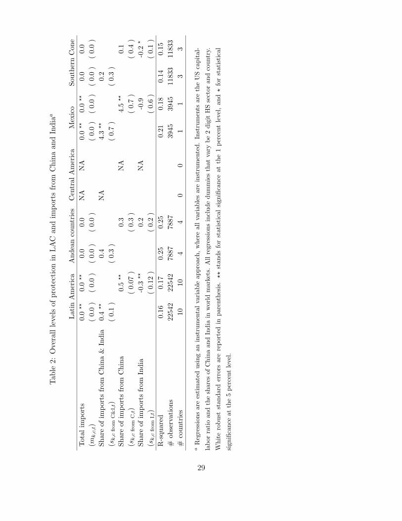
Does the pattern of higher protection applied to Chinese goods and lower protection
applied to Indian goods hold when we consider non tariff barriers as well? The answer is
positive and the results are reported in Table 2, where we use the same specification as in
Table 1, but add to the six digit Harmonized System tariffs the ad-valorem equivalents of non
tariff barriers obtained by Kee, Nicita and Olarreaga (2006).12 The statistical significance
of the estimates is not as high as for those in Table 1, but the same pattern is present. Note
that we do not have results for Central American countries, because there are no estimates
available for the trade restrictiveness of their non tariff barriers.13
In sum, sectors characterized by a larger share of imports from China tend to receive
higher protection, while sectors characterized by a larger share of imports from India tend
to face lower levels of protection. While we think that this evidence is per se important,
to provide an explanation for these patterns we extend the Grossman and Helpman (1994)
‘protection for sale’ model to allow for imperfect substitution between domestically produced
goods and imported goods. We then bring the extended model to the data.
11We have also experimented estimating equation (1) controlling for the presence of preferential tradeagreeements and for the accession of China as a WTO member. In the former case, we used fixed effects tocontrol for the presence of preferential agreeements. In the latter case, we have also used as an explanatoryvariable the interaction between the share of imports from China and a dummy variable which is equal toone after the year of 2000. The results described above remain intact and the regression results are availableupon request.
12Note that these estimates only exist for the year 2001, so we lost the time dimension in our sample.Results reported in Table 2 are for the year 2001 only.
13The first-stage regressions used to compute the results in table 2 are in general highly statisticallysignificant. The first-stage results are available upon reuqest.
8
3 Introducing imperfect substitution in the protection
for sale model
To analyze the political economy consequences of increased commercial ties with emerging
economies such as China and India, we consider a model in which a small open economy sets
trade policy vis-a-vis imports from the rest of the world (ROW). The key hypothesis in our
model is that goods are differentiated by location of origin, that is, we adopt the Armington
assumption and regard imports and domestically produced varieties as imperfect substitutes.
Our model features n + 1 different types of goods, and we allow each type to be produced
either domestically or imported from abroad. Later on we will allow for three different types
of imported goods, depending on whether they originate in India, China or elsewhere. The
extension is straightforward and thus to simplify the presentation of the extended model we
focus on a composite imported variety.14
Indicating by subscript k the type of good, consumers in the home country maximize the
following quasi-linear utility function:
U = X0 +n∑
k=1
Uk(Xk) (2)
where Uk(.) are strictly concave subutility functions (Uk = Ek ln Xk, that is, an upper tier
Cobb-Douglas) that depend on a CES aggregate of the imported and domestic variety of the
good, denoted with subscripts d and i respectively, i.e.
Xk =[x
ρkk,d + x
ρkk,i
] 1ρk 0 < ρk < 1 (3)
where xk,d stands for the consumption of the domestic variety of good k ∈ {1, ..., n}, xk,i
is the consumption of the imported variety, σk = 11−ρk
> 1 is the elasticity of substitution
between the two varieties, and good zero is the numeraire. Note that quasi–linearity implies
that there is neither an income nor a substitution effect for non-numeraire goods, as is
14Different varieties in a protection for sale model under monopolistic competition have been analyzed byChang (2005).
9
standard in the protection for sale model.
The supply side is a specific-factor model where the primary inputs are sector-specific
capital and mobile labor. Each individual in this economy is endowed with labor and at most
one sector–specific input. The specifics of supply in each sector are summarized by profit
functions πk(pk,d), where pk,d is the price of the domestic variety. To make things tractable,
we are going to work with linear supply schedules, i.e. we will assume that the profit functions
are quadratic. Production of good zero uses only labor under constant returns to scale, and
by appropriate choice of unit its price as well as the wage rate are normalized to one.
For an individual with income E the maximization of equation 2 subject to the budget
constraint E = X0 +∑n
k=1(pk,dxk,d + pk,ixk,i) yields the following demands for the domestic
and imported varieties of each product:
xk,d(pk,d, pk,i, Ek; ρk) =Ekp
1ρk−1
k,d
pρk
ρk−1
k,d + pρk
ρk−1
k,i
(4)
xk,i(pk,d, pk,i, Ek; ρk) =Ekp
1ρk−1
k,i
pρk
ρk−1
k,d + pρk
ρk−1
k,i
(5)
where pk,i = p∗k + tk is the price of the imported variety that results as the sum of the
exogenous world market price and the import tariff, and Ek is the expenditure on good k
(see the parameter of the Cobb-Douglas above). Note that — in line with a substantial part
of the literature and in view of the goal of this paper — we do not explicitly consider export
policies.
The price of the domestic variety results from the interplay of domestic supply and
domestic demand, where the latter varies not only with the price of the domestic variety
but also with the price of the imported variety, and this relation depends on the degree of
substitutability. In particular, setting demand equal supply in the market for the domestic
variety, i.e. xk,d(pk,d, pk,i, Ek; ρk) = π′(pk,d), implicitly defines the equilibrium price of the
domestic variety
10
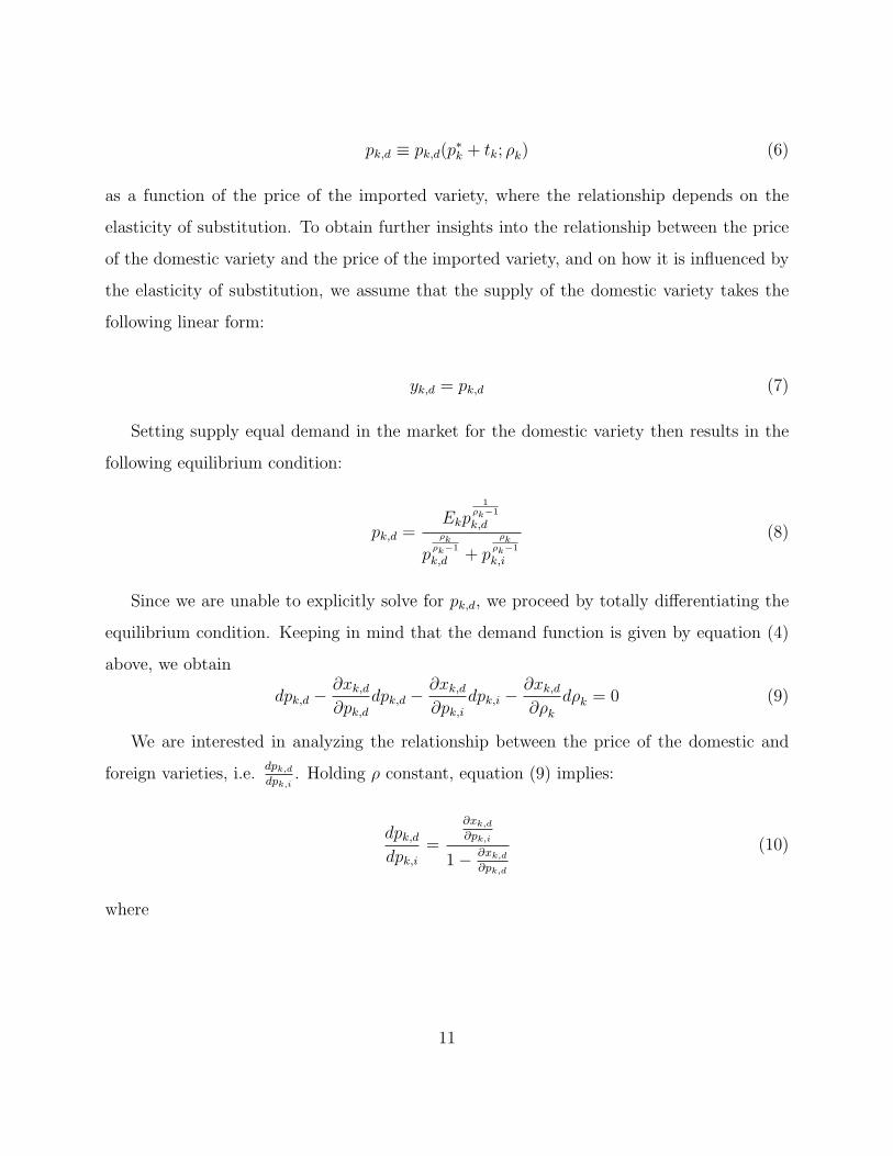
pk,d ≡ pk,d(p∗k + tk; ρk) (6)
as a function of the price of the imported variety, where the relationship depends on the
elasticity of substitution. To obtain further insights into the relationship between the price
of the domestic variety and the price of the imported variety, and on how it is influenced by
the elasticity of substitution, we assume that the supply of the domestic variety takes the
following linear form:
yk,d = pk,d (7)
Setting supply equal demand in the market for the domestic variety then results in the
following equilibrium condition:
pk,d =Ekp
1ρk−1
k,d
pρk
ρk−1
k,d + pρk
ρk−1
k,i
(8)
Since we are unable to explicitly solve for pk,d, we proceed by totally differentiating the
equilibrium condition. Keeping in mind that the demand function is given by equation (4)
above, we obtain
dpk,d −∂xk,d
∂pk,d
dpk,d −∂xk,d
∂pk,i
dpk,i −∂xk,d
∂ρk
dρk = 0 (9)
We are interested in analyzing the relationship between the price of the domestic and
foreign varieties, i.e.dpk,d
dpk,i. Holding ρ constant, equation (9) implies:
dpk,d
dpk,i
=
∂xk,d
∂pk,i
1− ∂xk,d
∂pk,d
(10)
where
11
∂xk,d
∂pk,i
= −ρk
ρk−1Ek(pk,dpk,i)
1ρk−1
[pρk
ρk−1
k,d + pρk
ρk−1
k,i ]2, (11)
and
∂xk,d
∂pk,d
=Ep
2ρk−1
k,d (1− ρk + (pk,d/pk,i)−ρkρk−1 )
[pρk
ρk−1
k,d + pρk
ρk−1
k,i ]2(ρk − 1)
, (12)
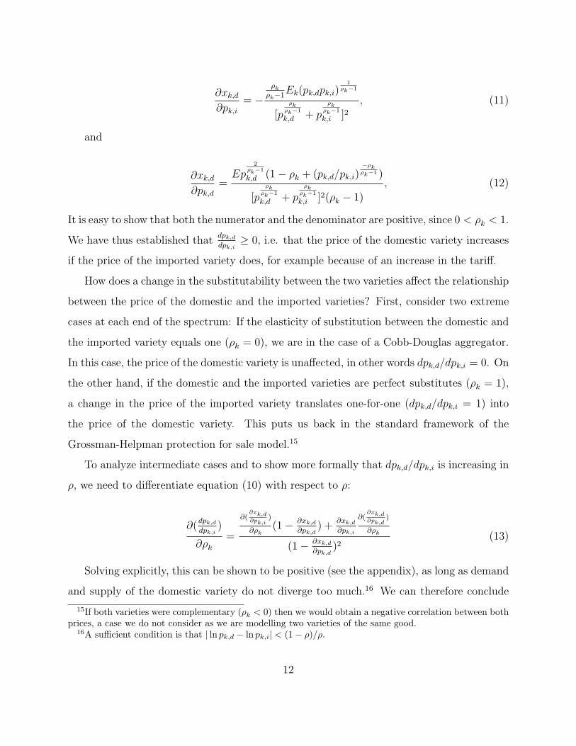
It is easy to show that both the numerator and the denominator are positive, since 0 < ρk < 1.
We have thus established thatdpk,d
dpk,i≥ 0, i.e. that the price of the domestic variety increases
if the price of the imported variety does, for example because of an increase in the tariff.
How does a change in the substitutability between the two varieties affect the relationship
between the price of the domestic and the imported varieties? First, consider two extreme
cases at each end of the spectrum: If the elasticity of substitution between the domestic and
the imported variety equals one (ρk = 0), we are in the case of a Cobb-Douglas aggregator.
In this case, the price of the domestic variety is unaffected, in other words dpk,d/dpk,i = 0. On
the other hand, if the domestic and the imported varieties are perfect substitutes (ρk = 1),
a change in the price of the imported variety translates one-for-one (dpk,d/dpk,i = 1) into
the price of the domestic variety. This puts us back in the standard framework of the
Grossman-Helpman protection for sale model.15
To analyze intermediate cases and to show more formally that dpk,d/dpk,i is increasing in
ρ, we need to differentiate equation (10) with respect to ρ:
∂(dpk,d
dpk,i)
∂ρk
=
∂(∂xk,d∂pk,i
)
∂ρk(1− ∂xk,d
∂pk,d) +
∂xk,d
∂pk,i
∂(∂xk,d∂pk,d
)
∂ρk
(1− ∂xk,d
∂pk,d)2
(13)
Solving explicitly, this can be shown to be positive (see the appendix), as long as demand
and supply of the domestic variety do not diverge too much.16 We can therefore conclude
15If both varieties were complementary (ρk < 0) then we would obtain a negative correlation between bothprices, a case we do not consider as we are modelling two varieties of the same good.
16A sufficient condition is that | ln pk,d − ln pk,i| < (1− ρ)/ρ.
12
that p′k ≡ dpk,d/dpk,i is a positive function of ρk.
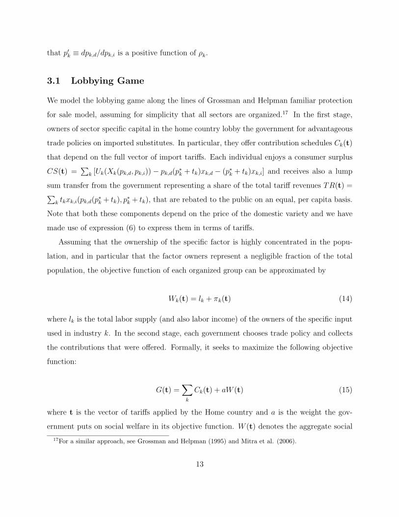
3.1 Lobbying Game
We model the lobbying game along the lines of Grossman and Helpman familiar protection
for sale model, assuming for simplicity that all sectors are organized.17 In the first stage,
owners of sector specific capital in the home country lobby the government for advantageous
trade policies on imported substitutes. In particular, they offer contribution schedules Ck(t)
that depend on the full vector of import tariffs. Each individual enjoys a consumer surplus
CS(t) =∑
k [Uk(Xk(pk,d, pk,i))− pk,d(p∗k + tk)xk,d − (p∗k + tk)xk,i] and receives also a lump
sum transfer from the government representing a share of the total tariff revenues TR(t) =∑k tkxk,i(pk,d(p
∗k + tk), p
∗k + tk), that are rebated to the public on an equal, per capita basis.
Note that both these components depend on the price of the domestic variety and we have
made use of expression (6) to express them in terms of tariffs.
Assuming that the ownership of the specific factor is highly concentrated in the popu-
lation, and in particular that the factor owners represent a negligible fraction of the total
population, the objective function of each organized group can be approximated by
Wk(t) = lk + πk(t) (14)
where lk is the total labor supply (and also labor income) of the owners of the specific input
used in industry k. In the second stage, each government chooses trade policy and collects
the contributions that were offered. Formally, it seeks to maximize the following objective
function:
G(t) =∑
k
Ck(t) + aW (t) (15)
where t is the vector of tariffs applied by the Home country and a is the weight the gov-
ernment puts on social welfare in its objective function. W (t) denotes the aggregate social
17For a similar approach, see Grossman and Helpman (1995) and Mitra et al. (2006).
13

welfare function, which is defined as follows:
W (t) = L +∑
k
πk(t) + CS(t) + TR(t) (16)
where L denotes the labor force (hence labor income because w = 1).
Because we do not have information on political organization by sector in Latin America
(i.e., there is no legal requirement for public disclosure of industries’ political contributions),
when solving for the optimal tariff we will assume that all industries are organized (which
is not unreasonable given the high level of industry aggregation in our data), and that
contribution functions are differentiable (i.e. locally truthful).
Taking the first order condition of the government’s maximization problem in (16), and
rearranging we obtain:
t0k1 + t0k
=1
a× zk
εk
× p′k (17)
where t0k ≡ tk/pk,i is the ad valorem tariff, zk ≡ xk,d/xk,i is the inverse import penetration
ratio, and εk is the total price elasticity of import demand that consists of the direct price
effect and the cross-price effect due to the tariff’s impact on the domestic price.18 The last
term is the main innovation vis-a-vis the standard model (p′k is given by equation (10)).
We have shown above that it depends positively on the elasticity of substitution. Thus in
the presence of high substitution between domestically produced goods and imported goods,
tariffs are likely to be higher.
4 Empirical Analysis
To assess the ability of our model to explain the patterns of protection towards Chinese
and Indian imports we have highlighted in our preliminary data analysis, we proceed in two
steps. First, we estimate the elasticity of substitution between the domestically produced
18Formally, εk = εk,i + εk,dεp,k = ∂xk,i
∂pk,i
pk,i
xk,i+ ∂xk,i
∂pk,d
pk,d
xk,i× ∂pk,d
∂pk,i
pk,i
pk,d.
14
variety of a given good and the varieties respectively imported from China, India and the
rest of the world. For our model to be compatible with the data, the estimated elasticity of
substitution between domestically produced and Chinese produced varieties should be higher
than the elasticity of substitution between the domestic variety and the variety imported
from the rest of the world. The opposite should hold for the Indian imported varieties.
Next, we compare the performance of our model against the standard Grossman and
Helpman benchmark. If product heterogeneity is important, we expect our model to fit
better the data than the standard benchmark.
4.1 Estimating the substitutability between domestically produced
goods and imports from China and India
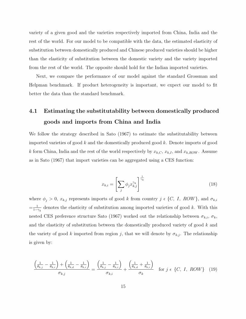
We follow the strategy described in Sato (1967) to estimate the substitutability between
imported varieties of good k and the domestically produced good k. Denote imports of good
k form China, India and the rest of the world respectively by xk,C , xk,I , and xk,ROW . Assume
as in Sato (1967) that import varieties can be aggregated using a CES function:
xk,i =
[∑j
φjxγkk,j
] 1γk
(18)
where φj > 0, xk,j represents imports of good k from country j ε {C, I, ROW}, and σk,i
= 11−γk
denotes the elasticity of substitution among imported varieties of good k. With this
nested CES preference structure Sato (1967) worked out the relationship between σk,i, σk,
and the elasticity of substitution between the domestically produced variety of good k and
the variety of good k imported from region j, that we will denote by σk,j. The relationship
is given by:
(1
θk,j− 1
θk,i
)+
(1
θk,d− 1
θk,i
)σk,j
=
(1
θk,j− 1
θk,i
)σk,i
+
(1
θk,d+ 1
θk,i
)σk
for j ε {C, I, ROW} (19)
15

where θk,j is the share of total expenditure on the imported variety of good k from region j,
θk,i is the share of total expenditure on imports of that good (i.e., θk,i =∑
j θk,j), and θk,d
is the share of total expenditure on the domestic variety of good k.
Using equation (5) we can derive the price elasticity of the composite of imported goods,
εk. Solving for σk we have σk = −εk. Thus, with an estimate of the price elasticity of the
imported composite good k that we can be borrow from the existing literature, we can derive
an estimate for σk. With data on σk and on the share of expenditure on domestic and on
imported varieties we can use the relationship described in equation (19) to obtain estimates
for the degree of substitutability between domestically produced goods and respectively
imports from China, India and the rest of the world.19
Before bringing equation (19) to the data, notice that the shares of expenditure on
domestic and imported varieties appear in the left and right-hand sides of expression (19).
Therefore, we need to rearrange the expression to be able to estimate the parameters of
interest. As a result, the equation to be estimated becomes:
1
σ= α1,j
(1
θk,d− 1
θk,i
)(
1θk,d
+ 1θk,i
) + α2,j
(1
θk,j− 1
θk,i
)(
1θk,d
+ 1θk,i
) + εk for j ε {C, I, ROW} (20)
where α1,j = 1σj
and α2,j =(
1σi− 1
σj
)are the parameters of interest, while εk is a zero mean
error term that captures measurement errors in the dependent variable. σj can be estimated
by calculating 1/α1,j. Expression (20) is the basis for our estimation of the relative degrees
of substitutability between the domestically produced and the goods imported from different
regions. Results are discussed in subsection 4.3.
4.2 Does the extended model perform better?
In order to assess whether the extended model with imperfect substitution between domes-
tically produced goods and imported goods performs better than the traditional ‘protection
19Note though that in our empirical analysis we will only be able to capture the average degree of substi-tutability σC , σI , and σROW , as we have too few observations to estimate sector specific elasticities.
16
for sale’ model with homogeneous goods, we will run both models on our sample of Latin
American countries: the extended model provided by equation (17) and the traditional model
where the last term in equation (17) is not present. We will then explore which of the two
models better explains Latin America’s tariff structure by comparing the R-squared of the
two regressions and by applying Davidson and MacKinnon (1981) non-nested J-test.20
We will also assess the two specifications in terms of their economic significance. One
problem with the empirical literature on the ‘protection for sale’ model is that the estimates
obtained for a, the parameter describing the weight attached by the government to aggregate
welfare, are unreasonably high (see Gawande and Krishna, 2004 for a survey of the empirical
literature). According to the existing estimates of the traditional ‘protection for sale’ model
with homogeneous goods, the weight attached by the government on industry lobbying when
setting trade policy represents less than 1 percent of the weight the government puts on social
welfare. This is hardly consistent with observed behavior and tariff structures. If we were
to obtain a lower, and more reasonable estimate for a when bringing our extended model to
the data, we would have evidence suggesting that our framework is also economically more
meaningful.
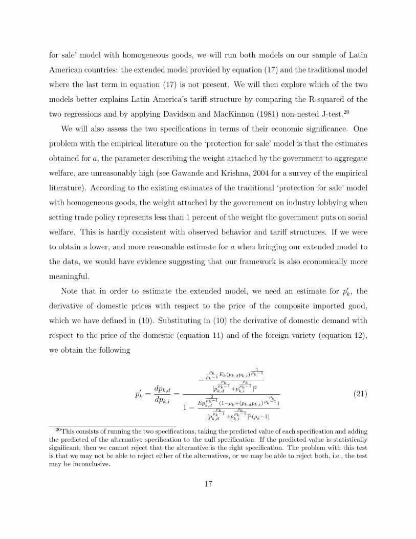
Note that in order to estimate the extended model, we need an estimate for p′k, the
derivative of domestic prices with respect to the price of the composite imported good,
which we have defined in (10). Substituting in (10) the derivative of domestic demand with
respect to the price of the domestic (equation 11) and of the foreign variety (equation 12),
we obtain the following
p′k =dpk,d
dpk,i
=
−ρk
ρk−1Ek(pk,dpk,i)
1ρk−1
[p
ρkρk−1
k,d +p
ρkρk−1
k,i ]2
1− Ep
2ρk−1
k,d (1−ρk+(pk,dpk,i)−ρkρk−1 )
[p
ρkρk−1
k,d +p
ρkρk−1
k,i ]2(ρk−1)
(21)
20This consists of running the two specifications, taking the predicted value of each specification and addingthe predicted of the alternative specification to the null specification. If the predicted value is statisticallysignificant, then we cannot reject that the alternative is the right specification. The problem with this testis that we may not be able to reject either of the alternatives, or we may be able to reject both, i.e., the testmay be inconclusive.
17

To be able to estimate p′k, we need data on the prices of the domestic and the composite
imported good, as well as consumer expenditure in sector k. The relative price between
the domestic good and the composite imported good is obtained using the two first order
conditions of the consumer maximization problem. More precisely, we take the ratio between
(4) and (5) and solve for the relative price. The quasi-linear structure of the theoretical
framework implies that there are neither income nor substitution effects for non-numeraire
goods. Thus, the model allows us to assume that the price of the imported good in every
sector is equal to one. Consumption is readily obtained from trade and production data.21
We use then equations (4) and (5) to calculate the price of the domestic varieties. One
concern we have when constructing p′k in this fashion is measurement error, but we instrument
the term p′k jointly with the rest of the right hand side term to address this problem.
Finally, a well-known problem with the estimation of the ‘protection for sale’ model in its
traditional or extended form is the endogeneity of the right-hand-side variables. In order to
correct for this we use as instruments China and India’s share in world trade by product, and
the capital-labor ratio of the United States in each industry. The results of the estimation of
the extended and traditional ‘protection for sale model’ as well as the first-stage regressions
are discussed in the next section (4.3).
4.3 Results
We start by discussing the results of the estimation of the degree of substitutability between
domestically produced goods and varieties that are imported from either China, India or the
rest of the world. We estimate equation (20) using data on imports from China, India, and
rest of the world separately. Parameter estimates obtained for equation (20), as well as the
implied σ’s are reported in Table 3. A quick look suggests that the degree of substitution
between Chinese goods and goods produced domestically in Latin America – as measured by
σC – is higher than the degree of substitution between goods imported from the rest of the
world and domestically produced goods – as measured by σROW – using data on the entire
21Or rather apparent consumption which equals imports plus domestic production minus exports.
18
sample of Latin American countries, on Andean countries and Southern cone countries. The
estimates for σC is numerically and statistically larger than the estimates for σROW , with
the exception of Mexico and Central America. The results for σI are statistically different
from zero in all regions, with the exception of Central America. However, the comparison
between σROW and σI does not generate a clear result, and in some cases the difference
between these parameters is not statistically different from zero.
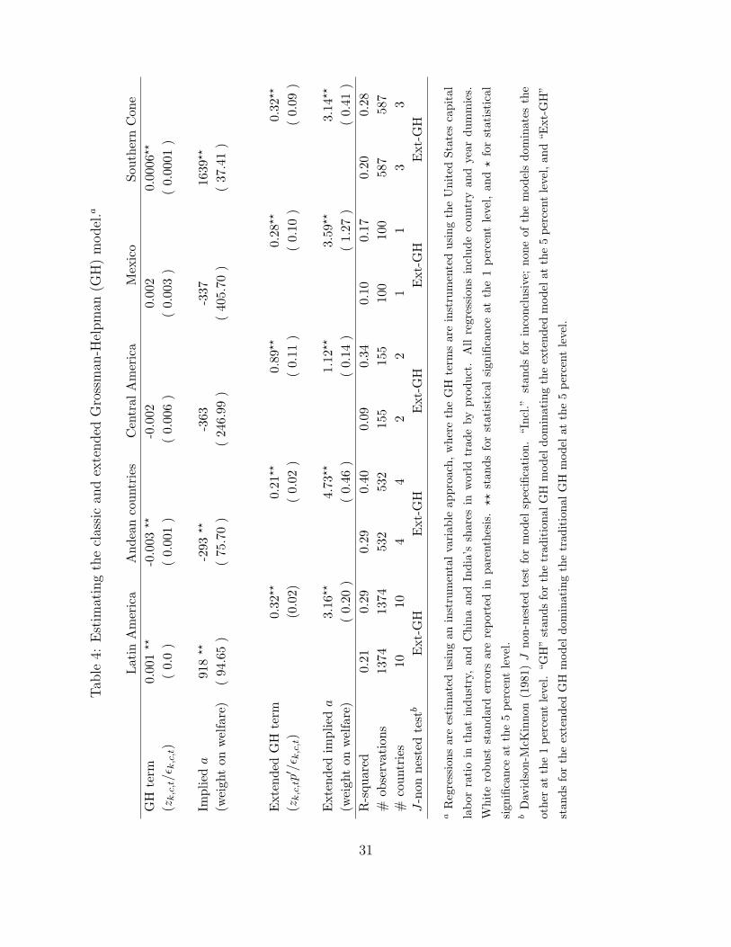
Table 4 provides the results of the estimation of (17) and the traditional ‘protection for
sale model’ for the entire pooled sample and the four sub-regions. Results for the pooled
sample, and for the Southern Cone always have the expected positive sign on the coefficient
of the GH term and of the extended GH term. For Andean countries, Central America, and
Mexico the coefficient is negative when using the traditional GH specification, which is at
odds with theory. This coefficient is instead positive for the extended GH specification, a
result that is consistent with our theoretical predictions. In fact, in all cases the extended
GH coefficient has the expected sign and is statistically different from zero.
Our results also suggest that the extended GH model performs better in terms of R-
squared, suggesting that the extended model that allows for imperfect substitutability be-
tween domestic and imported varieties fits better the data. The Davidson-McKinnon non-
nested J test for model specification indicates that the extended GH model dominates the
model with homogenous goods using either the pooled sample or the data by sub-regions.
As it can be seen from (17) the coefficient in front of the GH term (both in its traditional
and extended form) is given by 1/a, i.e., the inverse of the weight the government puts
on social welfare relative to industry lobbying when setting trade policy. In the case of the
extended GH model we obtain estimates for this parameter that are all positive (as expected)
and statistically different from zero.
More interestingly, the estimates for the weight the governments put on welfare relative
to industry lobbying are more realistic than the figures obtained in the existing literature. In
fact, for the extended GH model, they oscillate between 1 and 5, rather than ranging from
negative to between 900 and 1600 (or even negative) as in the traditional GH model. Allowing
19
for imperfect substitution between domestically produced goods and imported goods thus
provides one possible solution to the puzzle of large estimates of a. In fact, the results from
the traditional GH model would suggest that the relative weight the government puts on
industry lobbying is around 0.1 percent of the weight put on social welfare for the pooled
LAC sample (0.001 = 1/[a = 918])). If this were the case, assuming no other market
imperfections, it would be very difficult to explain the high levels of trade protection that
can be observed in Latin America. On the other hand, the estimates from the extended
GH model suggest that the weight attached by the government on industry lobbying is 32
percent of the weight it puts on social welfare (0.32 = 1/([a = 3.16])), suggesting a much
larger scope for lobbies’ influence. Governments with the least concern for social welfare are
to be found in Central America (where a is estimated at 1.12), and the governments with the
highest concern for social welfare are to be found among Andean countries with an average
a estimated at 4.73.22
Table 5 shows the first-stage regression results which were used to obtain the results
displayed in table 4. The F-statistics indicate that the instrumental variables used to estimate
the traditional GH model are statistically significant for the pooled sample, for the Andean
and for the Mercosur countries, and for Mexico. There is no evidence that the instrumental
variables are suitable in estimating the traditional GH model for Central American countries.
The F-test indicates that the instrumental variables are jointly significant for the pooled
sample and for all sub-region when estimating the extended GH model. In most cases, the
F-statistics is greater than 10 in the extended GH model’s first stage regressions. Since we
have a single endogenous regressor, these results reinforce our belief in the appropriateness
of the instrumental variables used to estimated the extended GH model.23
22We also estimate (17) and the traditional ‘protection for sale model’ using the overall level of protectionthat includes ad-valorem equivalents of non tariff barriers as the left hand side variable. Results for thepooled sample suggest that the parameter a equals 898 in the case of the traditional GH model, and is equalto 2.17 in the case of the extended GH model. However none of the estimates of the traditional GH modelare statistically different from zero (although they are different from each other). In the case of the extendedGH model, the estimates for the pooled sample as well as for Mercosur countries are statistically significantand have the expected sign. The results for the other sub-regions are not statistically significant.
23This observation follows from the “rule of thumb” suggested by Staiger and Stock (1997).
20
5 Conclusion
The growing presence of China and India in world markets and as a source for Latin American
imports has caught policy makers attention. This paper explores the response of Latin
American policy-makers to growing imports from China and India in their markets. We
found that sectors in which the share of imports from China is growing, generally tend to
have higher tariffs, controlling for reverse causality and industry, year and country effects.
The reverse pattern is observed in sectors where India’s presence is growing.
In order to explain this evidence, we develop an extension to the Grossman and Helpman
(1994) ‘protection for sale’ model to allow for imperfect substitution between domestically
produced goods and goods imported from different regions. The model suggest that as the
elasticity of substitution between domestically produced goods and imported goods increases,
the incentives to lobby also increase, and the resulting equilibrium tariff is higher.
Our analysis has been carried out in two steps. First, we have studied the substitutability
of domestically produced goods with imports from either China, India or the rest of the
world. We have found that Chinese imports are on average closer substitutes to goods
domestically produced in Latin America countries than goods originating in the rest of the
world, while the opposite is true for goods originating in India. Next, we have brought our
extended protection for sale framework to the data. We have shown that it outperforms the
traditional Grossman Helpman framework in two respects. First of all, it fits better the data.
Secondly, and even more interestingly, explicitly modeling imperfect substitutability between
domestic and imported varieties allows us to obtain substantially more realistic structural
parameter estimates than the ones obtained using an homogenous good specification.
A possible explanation for this result is that by ignoring the imperfect substitutability
between imported and domestically produced goods the existing literature is obtaining es-
timates for the weight attached by the government to aggregate welfare that are upward
biased. In fact, by assuming that imported goods and domestic varieties are perfect substi-
tutes, we would be led to conclude that the large variation observed in the political economy
term of the Grossman Helpman model (zk/εk) translates into a relatively small variation in
21
the level of protection because of the large weight attached by the government to aggregate
welfare. If we instead allow for our more general setting, the reason for which the govern-
ment does not react is not that it cares mainly about social welfare, but rather that there is
no lobbying pressure when imported goods are very imperfect substitutes for domestically
produced goods.
References
[1] Calderon, C., 2006. Trade, Specialization and Cycle Synchronization: Explaining Out-
put Comovement between Latin America, China and India. mimeo, The World Bank.
[2] Chang, P.L., 2005. Protection for sale under monopolistic competition. Journal of In-
ternational Economics 66 (2), 509-526.
[3] Davidson, R. and Mackinnon, J. G., 1981. Several tests for model specification in the
presence of alternative hypotheses. Econometrica 49(3), 781-793.
[4] Facchini G., Willmann G. and J. Van Biesebroeck, 2006 Protection for sale with imper-
fect rent capturing. Canadian Journal of Economics 39(3), 845–873.
[5] Gawande, K., 1997. Generated regressors in linear and non linear models. Economic
Letters 54(2), 119-126.
[6] Gawande, K., Bandhopadhyay, U., 2000. Is protection for sale? A test of the Grossman-
Helpman theory of endogenous protection. Review of Economics and Statistics 89(1),
139-152.
[7] Gawande, K., Krishna, P., 2004. The political economy of trade policy: empirical ap-
proaches. In: Choi, K., Harrigan, J. (Eds.), Handbook of International Trade. New
York: Basil Blackwell.
[8] Goldberg, P., Maggi, G., 1999. Protection for sale: an empirical investigation. American
Economic Review 89(5), 1135-1155.
22

[9] Grossman, G., Helpman, E., 1995. The politics of free trade agreement. American Eco-
nomic Review 85(4), 667–690.
[10] Grossman, G., Helpman, E., 1994. Protection for sale. American Economic Review
84(4), 833-850.
[11] Hoekman, B. M. and Kostecki M. M. 2001 The political economy of the world trading
system. Second Edition. Oxford University Press, Oxford and New York
[12] Kee, H.L., Nicita, A. and Olarreaga, M., 2004, Import demand elasticities and trade
distortions. Policy Research Working Paper #3452, The World Bank.
[13] Kee, H.L., Nicita, A. and Olarreaga, M., 2006, Estimating trade restrictiveness indices.
Policy Research Working paper # 3840, The World Bank.
[14] McCalman, Ph. 2004. Protection for Sale and Trade Liberalization: an Empirical In-
vestigation. Review of International Economics 12, 81-94.
[15] Mitra, D., 1999. Endogenous lobby formation and endogenous protection: a long-run
model of trade policy determination. American Economic Review 89(5), 1116-1134.
[16] Mitra, Devashish, Thomakos, D. and Ulubasoglu, M., 2002. Protection for sale in a
developing country: democracy versus dictatorship. Review of Economics and Statistics
84.
[17] Mitra, Devashish, Thomakos, D. and Ulubasoglu, M., 2006. Can we obtain realistic
estimates for the ’prtection for sale’ model? Canadian Journal of Economics 39: 187–
210
[18] Nicita, A. and Olarreaga, M., 2006. Trade, production and protection, 1976-2004.
Mimeo, The World Bank (available at www.worldbank.org/trade).
[19] Sato, K., 1967. A Two-Level Constant-Elasticity-of-Substitution Production Function.
Review of Economic Studies 34(2), 201-218.
23
[20] Staiger, D., and Stock, J. H., 1997. Instrumental Variables Regression with Weak In-
struments. Econometrica 65, 557 - 586.
24

Appendix
There are two parts to this appendix. First, we calculate the derivative of the domestic
prices with respect to the degree of substitutability between domestically produced goods
and imported goods. Second, we describe the data used in our analysis.
Derivative of p′k with respect to ρk
Differentiating (21) with respect to ρk, setting all international prices equal to 1, and denoting
pk = pk,d/pk,i as the relative price of domestic to imported goods yields:
∂p′k∂ρk
= Ekpρk+1
ρk−1
k
[(Ekp
2ρk−1
k + p2ρk
ρk−1
k
)(ρk − 1)− p
ρkρk−1
k
(Ekp
2ρk−1
k
+ 2p2ρk
ρk−1
k
)(1− ρk + ρklog(pk)) + p
ρkρk−1
k (ρk − 1 + ρklog(pk))
]/
[p
3ρkρk−1
k (ρk − 1)− Ekp2
ρk−1
k + 2p2ρk
ρk−1
k (ρk − 1)
+ pρk
ρk−1
k
(Ekp
2ρk−1
k + 1
)(ρk − 1)
]2
(ρk − 1) (22)
And it can be shown that a sufficient condition for the right hand side of (22) to be positive
is log(pk) = log(pk,d)− log(pk,i) < (1− ρk)/ρk. To see this note that the denominator is non-
positive as ρk ≤ 1. The first two terms in the squared parenthesis are also non-positive as
long as log(pk) > 0 (which will be the case in this world with horizontal differentiation and
tariffs on imported goods). Thus, a sufficient condition is that the third term in the squared
parenthesis in the numerator is negative. And this will be the case if log(pk) =< (1−ρk)/ρk.
25
Data Appendix
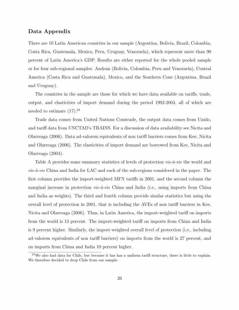
There are 10 Latin American countries in our sample (Argentina, Bolivia, Brazil, Colombia,
Costa Rica, Guatemala, Mexico, Peru, Uruguay, Venezuela), which represent more than 90
percent of Latin America’s GDP. Results are either reported for the whole pooled sample
or for four sub-regional samples: Andean (Bolivia, Colombia, Peru and Venezuela), Central
America (Costa Rica and Guatemala), Mexico, and the Southern Cone (Argentina, Brazil
and Uruguay).
The countries in the sample are those for which we have data available on tariffs, trade,
output, and elasticities of import demand during the period 1992-2004, all of which are
needed to estimate (17).24
Trade data comes from United Nations Comtrade, the output data comes from Unido,
and tariff data from UNCTAD’s TRAINS. For a discussion of data availability see Nicita and
Olarreaga (2006). Data ad-valorem equivalents of non tariff barriers comes from Kee, Nicita
and Olarreaga (2006). The elasticities of import demand are borrowed from Kee, Nicita and
Olarreaga (2004).
Table A provides some summary statistics of levels of protection vis-a-vis the world and
vis-a-vis China and India for LAC and each of the sub-regions considered in the paper. The
first column provides the import-weighted MFN tariffs in 2001, and the second column the
marginal increase in protection vis-a-vis China and India (i.e., using imports from China
and India as weights). The third and fourth column provide similar statistics but using the
overall level of protection in 2001, that is including the AVEs of non tariff barriers in Kee,
Nicita and Olarreaga (2006). Thus, in Latin America, the import-weighted tariff on imports
from the world is 13 percent. The import-weighted tariff on imports from China and India
is 9 percent higher. Similarly, the import-weighted overall level of protection (i.e., including
ad-valorem equivalents of non tariff barriers) on imports from the world is 27 percent, and
on imports from China and India 10 percent higher.
24We also had data for Chile, but because it has has a uniform tariff structure, there is little to explain.We therefore decided to drop Chile from our sample.
26

Table A: Average Levels of protection vis-a-vis the world, and China and India in 2001.a
Tariffs, 2001 Overall level of protection, 2001
World China & India World China & India
Andean countries 11 +26% 23 -4%
Central America 5 +66% NA NA
Mexico 11 +13% 24 +9%
Southern Cone 15 +9% 30 +19%
Latin America 13 +9% 27 +10%
aAll averages are import-weighted. For China and India, we provide the change in protection with respectto the MFN levels in percentages.
27

Tab
le1:
Tar
iffs
inLA
Can
dim
por
tsfr
omC
hin
aan
dIn
dia
a
Lat
inA
mer
ica
And
ean
coun
trie
sC
entr
alA
mer
ica
Mex
ico
Sout
hern
Con
eTot
alim
port
s0.
14??
0.94
??
0.1
??
4.0
??
-0.2
??
-0.2
??
0.01
??
0.02
??
0.07
??
0.08
??
(mk,c
,t)
(0.
01)
(0.
01)
(0.
02)
(0.
09)
(0.
05)
(0.
06)
(0.
00)
(0.
00)
(0.
01)
(0.
02)
Shar
eof
impo
rts
from
Chi
na&
Indi
a0.
8??
0.25
??
-2.2
8??
0.59
??
0.4
??
(sk,c
from
C&
I,t)
(0.
04)
(0.
03)
(0.
09)
(0.
08)
(0.
04)
Shar
eof
impo
rts
from
Chi
na4.
52??
6.45
??
-2.7
??
1.12
??
3.8
??
(sk,c
from
C,t)
(0.
05)
(0.
16)
(0.
11)
(0.
09)
(0.
08)
Shar
eof
impo
rts
from
Indi
a-0
.05
??
-0.1
3??
-0.4
3-0
.21
??
-0.1
??
(sk,c
from
I,t)
(0.
01)
(0.
02)
(0.
25)
(0.
05)
(0.
02)
R-s
quar
ed0.
550.
570.
670.
680.
650.
650.
560.
570.
630.
64#
obse
rvat
ions
2478
2224
7822
1010
1010
1010
3421
534
215
2267
622
676
8992
189
921
#co
untr
ies
1010
44
22
11
33
aR
egre
ssio
nsar
ees
tim
ated
usin
gan
inst
rum
enta
lva
riab
leap
proa
ch,
whe
real
lva
riab
les
are
inst
rum
ente
d.In
stru
men
tsar
eth
esh
ares
of
Chi
naan
dIn
dia
inw
orld
mar
kets
,an
dth
eU
Sca
pita
l-la
bor
rati
o.A
llre
gres
sion
sin
clud
edu
mm
ies
that
vary
be2
digi
tH
Sse
ctor
,ye
aran
d
coun
try.
Whi
tero
bust
stan
dard
erro
rsar
ere
port
edin
pare
nthe
sis.
??st
ands
for
stat
isti
cal
sign
ifica
nce
atth
e1
perc
ent
leve
l,an
d?
for
stat
isti
calsi
gnifi
canc
eat
the
5pe
rcen
tle
vel.
28
Tab
le2:
Ove
rall
leve
lsof
pro
tect
ion
inLA
Can
dim
por
tsfr
omC
hin
aan
dIn
dia
a
Lat
inA
mer
ica
And
ean
coun
trie
sC
entr
alA
mer
ica
Mex
ico
Sout
hern
Con
eTot
alim
port
s0.
0??
0.0
??
0.0
0.0
NA
NA
0.0
??
0.0
??
0.0
0.0
(mk,c
,t)
(0.
0)
(0.
0)
(0.
0)
(0.
0)
(0.
0)
(0.
0)
(0.
0)
(0.
0)
Shar
eof
impo
rts
from
Chi
na&
Indi
a0.
4??
0.4
NA
4.3
??
0.2
(sk,c
from
C&
I,t)
(0.
1)
(0.
3)
(0.
7)
(0.
3)
Shar
eof
impo
rts
from
Chi
na0.
5??
0.3
NA
4.5
??
0.1
(sk,c
from
C,t)
(0.
07)
(0.
3)
(0.
7)
(0.
4)
Shar
eof
impo
rts
from
Indi
a-0
.3??
0.2
NA
-0.9
-0.2
?
(sk,c
from
I,t)
(0.
12)
(0.
2)
(0.
6)
(0.
1)
R-s
quar
ed0.
160.
170.
250.
250.
210.
180.
140.
15#
obse
rvat
ions
2254
222
542
7887
7887
3945
3945
1183
311
833
#co
untr
ies
1010
44
00
11
33
aR
egre
ssio
nsar
ees
tim
ated
usin
gan
inst
rum
enta
lva
riab
leap
proa
ch,w
here
allva
riab
les
are
inst
rum
ente
d.In
stru
men
tsar
eth
eU
Sca
pita
l-
labo
rra
tio
and
the
shar
esof
Chi
naan
dIn
dia
inw
orld
mar
kets
.A
llre
gres
sion
sin
clud
edu
mm
ies
that
vary
be2
digi
tH
Sse
ctor
and
coun
try.
Whi
tero
bust
stan
dard
erro
rsar
ere
port
edin
pare
nthe
sis.
??st
ands
for
stat
isti
cal
sign
ifica
nce
atth
e1
perc
ent
leve
l,an
d?
for
stat
isti
cal
sign
ifica
nce
atth
e5
perc
ent
leve
l.
29
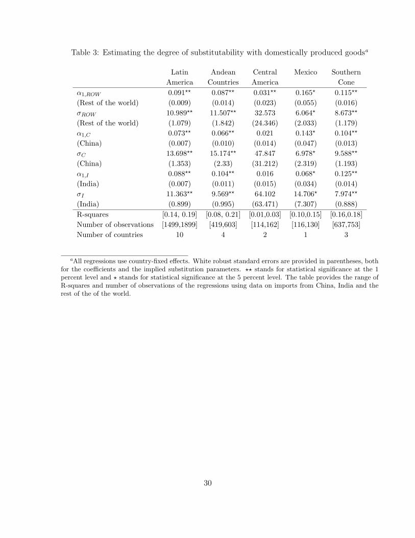
Table 3: Estimating the degree of substitutability with domestically produced goodsa
Latin Andean Central Mexico SouthernAmerica Countries America Cone
α1,ROW 0.091?? 0.087?? 0.031?? 0.165? 0.115??
(Rest of the world) (0.009) (0.014) (0.023) (0.055) (0.016)σROW 10.989?? 11.507?? 32.573 6.064? 8.673??
(Rest of the world) (1.079) (1.842) (24.346) (2.033) (1.179)α1,C 0.073?? 0.066?? 0.021 0.143? 0.104??
(China) (0.007) (0.010) (0.014) (0.047) (0.013)σC 13.698?? 15.174?? 47.847 6.978? 9.588??
(China) (1.353) (2.33) (31.212) (2.319) (1.193)α1,I 0.088?? 0.104?? 0.016 0.068? 0.125??
(India) (0.007) (0.011) (0.015) (0.034) (0.014)σI 11.363?? 9.569?? 64.102 14.706? 7.974??
(India) (0.899) (0.995) (63.471) (7.307) (0.888)R-squares [0.14, 0.19] [0.08, 0.21] [0.01,0.03] [0.10,0.15] [0.16,0.18]Number of observations [1499,1899] [419,603] [114,162] [116,130] [637,753]Number of countries 10 4 2 1 3
aAll regressions use country-fixed effects. White robust standard errors are provided in parentheses, bothfor the coefficients and the implied substitution parameters. ?? stands for statistical significance at the 1percent level and ? stands for statistical significance at the 5 percent level. The table provides the range ofR-squares and number of observations of the regressions using data on imports from China, India and therest of the of the world.
30
Tab
le4:
Est
imat
ing
the
clas
sic
and
exte
nded
Gro
ssm
an-H
elpm
an(G
H)
model
.a
Lat
inA
mer
ica
And
ean
coun
trie
sC
entr
alA
mer
ica
Mex
ico
Sout
hern
Con
eG
Hte
rm0.
001
??
-0.0
03??
-0.0
020.
002
0.00
06??
(zk,c
,t/ε
k,c
,t)
(0.
0)
(0.
001
)(
0.00
6)
(0.
003
)(
0.00
01)
Impl
ied
a91
8??
-293
??
-363
-337
1639
??
(wei
ght
onw
elfa
re)
(94
.65
)(
75.7
0)
(24
6.99
)(
405.
70)
(37
.41
)
Ext
ende
dG
Hte
rm0.
32??
0.21
??
0.89
??
0.28
??
0.32
??
(zk,c
,tp′ /
ε k,c
,t)
(0.0
2)(
0.02
)(
0.11
)(
0.10
)(
0.09
)
Ext
ende
dim
plie
da
3.16
??
4.73
??
1.12
??
3.59
??
3.14
??
(wei
ght
onw
elfa
re)
(0.
20)
(0.
46)
(0.
14)
(1.
27)
(0.
41)
R-s
quar
ed0.
210.
290.
290.
400.
090.
340.
100.
170.
200.
28#
obse
rvat
ions
1374
1374
532
532
155
155
100
100
587
587
#co
untr
ies
1010
44
22
11
33
J-n
onne
sted
test
bE
xt-G
HE
xt-G
HE
xt-G
HE
xt-G
HE
xt-G
H
aR
egre
ssio
nsar
ees
tim
ated
usin
gan
inst
rum
enta
lva
riab
leap
proa
ch,w
here
the
GH
term
sar
ein
stru
men
ted
usin
gth
eU
nite
dSt
ates
capi
tal
labo
rra
tio
inth
atin
dust
ry,
and
Chi
naan
dIn
dia’
ssh
ares
inw
orld
trad
eby
prod
uct.
All
regr
essi
ons
incl
ude
coun
try
and
year
dum
mie
s.
Whi
tero
bust
stan
dard
erro
rsar
ere
port
edin
pare
nthe
sis.
??st
ands
for
stat
isti
cal
sign
ifica
nce
atth
e1
perc
ent
leve
l,an
d?
for
stat
isti
cal
sign
ifica
nce
atth
e5
perc
ent
leve
l.b
Dav
idso
n-M
cKin
non
(198
1)J
non-
nest
edte
stfo
rm
odel
spec
ifica
tion
.“I
ncl.”
stan
dsfo
rin
conc
lusi
ve;
none
ofth
em
odel
sdo
min
ates
the
othe
rat
the
1pe
rcen
tle
vel.
“GH
”st
ands
for
the
trad
itio
nalG
Hm
odel
dom
inat
ing
the
exte
nded
mod
elat
the
5pe
rcen
tle
vel,
and
“Ext
-GH
”
stan
dsfo
rth
eex
tend
edG
Hm
odel
dom
inat
ing
the
trad
itio
nalG
Hm
odel
atth
e5
perc
ent
leve
l.
31

Tab
le5:
First
-Sta
geR
esult
s.a
Lat
inA
mer
ica
And
ean
coun
trie
sC
entr
alA
mer
ica
Mex
ico
Sout
hern
Con
eG
HE
xt-G
HG
HE
xt-G
HG
HE
xt-G
HG
HE
xt-G
HG
HE
xt-G
HU
SK
/L0.
00??
0.00
??
0.00
∗∗0.
00∗∗
-0.0
00.
000.
000.
000.
00∗
0.00
(0.
00)
(0.
00)
(0.
00)
(0.
00)
(0.
00)
(0.
00)
(0.
00)
(0.
00)
(0.
00)
(0.
00)
Chi
na’s
wor
ldsh
are
218.
67??
1.02
??
17.6
11.
17∗∗
-25.
420.
51∗
-2.0
00.
7760
0.74
??
1.08
∗∗
(70
.66
)(
0.14
)(1
4.00
)(
0.24
)(
38.7
8)
(0.
27)
(23
.30
)(
0.62
)(1
43.9
8)
(0.
23)
Indi
a’s
wor
ldsh
are
-739
.48∗∗
0.96
??
-104
.97∗∗
1.20
-211
.40
0.80
-206
.90
??
-2.2
0-1
570.
25∗∗
1.04
(16
6.42
)(
0.44
)(
34.5
2)
(0.
67)
(14
8.08
)(
0.90
)(
80.1
1)
(1.
84)
(36
4.83
)(
0.73
)
Con
stan
t4.
52∗
0.04
??
7.00
∗∗0.
02∗∗
4.72
∗∗0.
027.
94??
0.15
??
3.02
0.06
∗∗
(2.
08)
(0.
01)
(1.
22)
(0.
01)
(1.
41)
(0.
01)
(2.
08)
(0.
05)
(4.
24)
(4.
38)
F7.
07??
38.5
7??
4.58
??
14.2
4??
2.25
3.08
∗2.
98∗
2.14
6.33
??
23.0
4??
#ob
serv
atio
ns13
7413
7453
253
215
515
510
010
058
758
7#
coun
trie
s10
104
42
21
13
3
aW
hite
robu
stst
anda
rder
rors
are
repo
rted
inpa
rent
hesi
s.??
stan
dsfo
rst
atis
tica
lsi
gnifi
canc
eat
the
1pe
rcen
tle
vel,
and
?fo
rst
atis
tica
l
sign
ifica
nce
atth
e5
perc
ent
leve
l.
32