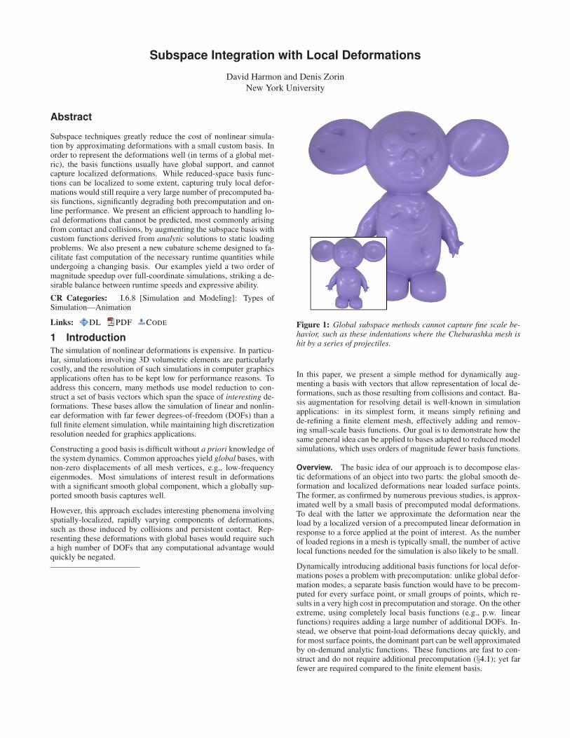
Subspace Integration with Local Deformations

David Harmon and Denis Zorin

New York University

Abstract

Subspace techniques greatly reduce the cost of nonlinear simula-tion by approximating deformations with a small custom basis. Inorder to represent the deformations well (in terms of a global met-ric), the basis functions usually have global support, and cannotcapture localized deformations. While reduced-space basis func-tions can be localized to some extent, capturing truly local defor-mations would still require a very large number of precomputed ba-sis functions, significantly degrading both precomputation and on-line performance. We present an efficient approach to handling lo-cal deformations that cannot be predicted, most commonly arisingfrom contact and collisions, by augmenting the subspace basis withcustom functions derived from analytic solutions to static loadingproblems. We also present a new cubature scheme designed to fa-cilitate fast computation of the necessary runtime quantities whileundergoing a changing basis. Our examples yield a two order ofmagnitude speedup over full-coordinate simulations, striking a de-sirable balance between runtime speeds and expressive ability.

CR Categories: I.6.8 [Simulation and Modeling]: Types ofSimulation—Animation

Links: DL PDF CODE

1 IntroductionThe simulation of nonlinear deformations is expensive. In particu-lar, simulations involving 3D volumetric elements are particularlycostly, and the resolution of such simulations in computer graphicsapplications often has to be kept low for performance reasons. Toaddress this concern, many methods use model reduction to con-struct a set of basis vectors which span the space of interesting de-formations. These bases allow the simulation of linear and nonlin-ear deformation with far fewer degrees-of-freedom (DOFs) than afull finite element simulation, while maintaining high discretizationresolution needed for graphics applications.

Constructing a good basis is difficult without a priori knowledge ofthe system dynamics. Common approaches yield global bases, withnon-zero displacements of all mesh vertices, e.g., low-frequencyeigenmodes. Most simulations of interest result in deformationswith a significant smooth global component, which a globally sup-ported smooth basis captures well.

However, this approach excludes interesting phenomena involvingspatially-localized, rapidly varying components of deformations,such as those induced by collisions and persistent contact. Rep-resenting these deformations with global bases would require sucha high number of DOFs that any computational advantage wouldquickly be negated.

Figure 1: Global subspace methods cannot capture fine scale be-havior, such as these indentations where the Cheburashka mesh ishit by a series of projectiles.

In this paper, we present a simple method for dynamically aug-menting a basis with vectors that allow representation of local de-formations, such as those resulting from collisions and contact. Ba-sis augmentation for resolving detail is well-known in simulationapplications: in its simplest form, it means simply refining andde-refining a finite element mesh, effectively adding and remov-ing small-scale basis functions. Our goal is to demonstrate how thesame general idea can be applied to bases adapted to reduced modelsimulations, which uses orders of magnitude fewer basis functions.

Overview. The basic idea of our approach is to decompose elas-tic deformations of an object into two parts: the global smooth de-formation and localized deformations near loaded surface points.The former, as confirmed by numerous previous studies, is approx-imated well by a small basis of precomputed modal deformations.To deal with the latter we approximate the deformation near theload by a localized version of a precomputed linear deformation inresponse to a force applied at the point of interest. As the numberof loaded regions in a mesh is typically small, the number of activelocal functions needed for the simulation is also likely to be small.

Dynamically introducing additional basis functions for local defor-mations poses a problem with precomputation: unlike global defor-mation modes, a separate basis function would have to be precom-puted for every surface point, or small groups of points, which re-sults in a very high cost in precomputation and storage. On the otherextreme, using completely local basis functions (e.g., p.w. linearfunctions) requires adding a large number of additional DOFs. In-stead, we observe that point-load deformations decay quickly, andfor most surface points, the dominant part can be well approximatedby on-demand analytic functions. These functions are fast to con-struct and do not require additional precomputation (§4.1); yet farfewer are required compared to the finite element basis.

Prior work in subspace integration has taken great pains to maintaina computational complexity that is a small power of the number ofbasis vectors. This is made possible by significant precomputa-tion that can easily be ruined by the introduction of dynamic bases(§5.1). We show that for the problem of local deformations we canmaintain the reduced complexity needed for interactive simulationsin two ways: our subspace DOFs are output-sensitive to the numberof loaded regions in the model, which is in most cases small (§4.2),and we use a novel cubature sampling strategy that takes advantageof the structure of loaded surfaces (§5.2).

We demonstrate dynamically generated subspace bases for defor-mations arising from transient collisions and persistent contact. Ourlocal subspace addition introduces only a modest computationalburden, yielding a two order of magnitude speedup speedup overfull-coordinate simulations for our examples (§7).

2 Related work

Subspace integration techniques have a long history in engineer-ing [Nickell 1976; Bathe and Gracewski 1981], with modal analy-sis a popular method for construction of a reduced basis [Thomson2004]. Later, these ideas were introduced to the graphics commu-nity by Pentland and Williams [1989], and extended to the non-linear regime by Barbic and James [2005], which built on similarwork from engineering [Idelsohn and Cardona 1985b].

Moving beyond linear modal analysis, Barbic and James [2005]expanded the concept of modal derivatives to represent large defor-mations and experimented with custom bases derived from sampleforces and offline static solutions. Example-based shape synthesishas been a popular research topic [Koyama et al. 2012; Martin et al.2011], however these methods are dependent on the quality of thetraining data provided.

Kim and James [2011] perform a domain decomposition withmodal analysis on each domain, which are then coupled togetherat boundaries, allowing restricting deformations to precomputeddomains. Truly local displacements, however, cannot be repre-sented unless decomposition is performed at a prohibitively finelevel. Barbic and Zhao [2011] build a hierarchy out of mesh com-ponents, with impulses transferred through the (small) interfacesdown the hierarchy. This allows somewhat local displacements, butagain limited to the mesh partitioning and specific mesh types thatadmit this type of substructuring.

Idelsohn and Cardona [1985a] compute new basis vectors dynami-cally, while Kim and James [2009] perform online model reductionto adaptively sample a precomputed basis. While not intended forlocal deformations, we make use of several ideas from this paper todynamically adapt a basis on-the-fly to external stimulii.

Ogot et al. [1996] proposed a hybrid simulation that uses rigid bodydynamics for free flight and explicit finite elements during the con-tact phase. At a high level this is similar to our approach, but weare not limited to purely rigid motion and do not resort to full finiteelements during contact, avoiding the limitations of both ends.

Adaptive refinement in finite element simulations has been an ac-tively studied topic in both engineering and graphics [Debunneet al. 2001; Wu et al. 2001; Grinspun et al. 2002]. In contrast tothese methods, which begin with a full-coordinate basis and thenrefine/coarsen, we begin with a modal basis and then dynamicallybuild local modes from displacement fields. Our approach requiressignificantly fewer basis functions (Fig. 3), and is not as dependenton the underlying mesh geometry.

An et al. [2008] developed a cubature scheme for approximatingintegrals across a mesh using a small set of representative ele-

ments. Our work uses cubature as well, but instead of an expensiveprecomputation, we construct our representative set and cubatureweights dynamically.

In graphics, simulating elastic objects independent of an underly-ing mesh has been an active topic of research. Point-based meth-ods [Gerszewski et al. 2009] as well as meshless methods [Faureet al. 2011] are popular alternatives. Previous work in precomputedGreen’s functions [James and Pai 2003], analytic solutions, such asthe Boussinesq solution [Pauly et al. 2004], and fundamental so-lutions to Navier’s equations [James and Pai 1999] are all similarin spirit to our method: using precomputed (or analytic) responsefunctions to accelerate online computation.

3 Subspace integration

The second order Euler-Lagrange equations describe the motion ofa deformable object:

Mu+D(u, u) +R(u) = f , (1)

where M is the system mass matrix, u is the vector of displace-ments, D,R, and f denote damping, internal, and external forces,respectively, and dots denote time derivatives.

In model reduction, the displacement vector is represented in a re-duced set of coordinates,

u = Uq,

where U ∈ R3n,r is a matrix with columns corresponding to the

vectors of the reduced displacement basis and q ∈ Rr is the vector

of reduced coordinates. The dimension of the subspace r is chosento be much less than 3n. Substituting u = Uq into Eqn. (1) wearrive at the reduced equations of motion, approximating (1) withfar fewer degrees-of-freedom:

Mq+ D(q, q) + R(q) = f , (2)

where a tilde denotes a reduced quantity, obtained by projecting into

the chosen subspace: M = UTMU, D(q, q) = UTD(Uq,Uq),

R(q) = UTR(Uq) and f = UT f .

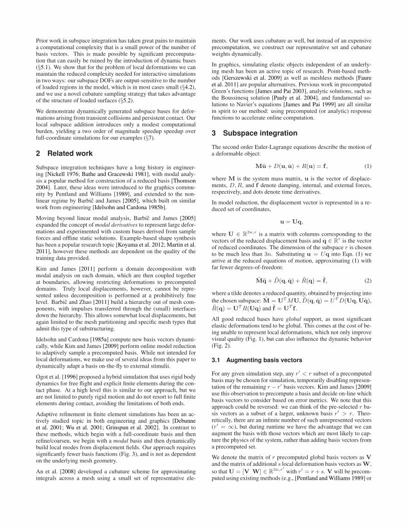
All good reduced bases have global support, as most significantelastic deformations tend to be global. This comes at the cost of be-ing unable to represent local deformations, which not only improvevisual quality (Fig. 1), but can also influence the dynamic behavior(Fig. 2).

3.1 Augmenting basis vectors

For any given simulation step, any r′ < r subset of a precomputedbasis may be chosen for simulation, temporarily disabling represen-tation of the remaining r− r′ basis vectors. Kim and James [2009]use this observation to precompute a basis and decide on-line whichbasis vectors to consider based on error metrics. We note that thisapproach could be reversed: we can think of the pre-selected r ba-sis vectors as a subset of a larger, unknown basis r′ > r. Theo-retically, there are an infinite number of such unrepresented vectors(r′ = ∞), but during runtime we have the advantage that we canaugment the basis with those vectors which are most likely to cap-ture the physics of the system, rather than adding basis vectors froma precomputed set.

We denote the matrix of r precomputed global basis vectors as Vand the matrix of additional s local deformation basis vectors as W,

so that U = [V W] ∈ R3n,r′ with r′ = r+ s. V will be precom-

puted using existing methods (e.g., [Pentland and Williams 1989] or

Figure 2: Local deformations can also significantly effect the simulation dynamics. A spikey box is dropped under gravity between twounfortunately-spaced cylinders. A global subspace cannot represent the local deformations needed to allow the box to slip between theobstacles. The local subspace method better approximates the overall behavior of the full-coordinate simulation.

global

local

hierarchical

f(x)

Figure 3: Representing the 1D function f(x) using a hierarchicalor subdivided basis would require an excessive number of basisfunctions, whereas a global basis combined with a shape-awarelocal basis can accurately capture the configuration with only afew basis functions.

[Barbic and James 2005]). W will be dynamically updated basedon the forces present in the system. Our focus is on deformationsdue to local forces, hence in the next section we show how to com-pute basis vectors in W in response to locally applied loads.

4 Local basis functions

We consider the specific case of augmenting a basis in order to rep-resent displacements from surface loads on the boundary of an ob-ject. This includes many interactive tools as well as deformationarising from collisions and contact. The only restriction we placeon these loads is that the resulting displacements are small enoughto be described by linear elasticity. Note, however, that this dis-placement is relative to existing modal deformations, so that in ag-gregate any node may experience quite large displacements.

4.1 Generating local basis vectors

The most direct way to augment a basis with local basis functionsis to use a local finite element basis, e.g., adding hat functions atthe nodes in the region of interest. The main problem of such astrategy is the number of basis functions that would be required torepresent even modest displacements (see Fig. 3). Not only wouldthree degrees of freedom be required per displaced surface node,but interior nodes must also be included for a reasonable represen-tation of displacement dynamics. In many cases these additionalbases have to cover a significant fraction of the mesh for faithfulrepresentation of deformations. Instead, we observe that the loads

of interest are often localized, thus, the load can be approximatedwell by a small number of local functions, while the deformationresponse can be approximated by the solutions of static elasticityproblems with point loads. Our idea is to adapt solutions to suchproblems, in the cases when these can be obtained analytically, foruse as additional basis functions.

Solutions to boundary load problems. Let f be a given loadon a single vertex, i.e., zero everywhere except for the vertex ofinterest. The exact solution for a given load f of a linear elasticityproblem is the solution u to the following linear equations:

Ku = f , (3)

where K is the 3n×3n Jacobian of R (Eqn. (1)), the FEM stiffnessmatrix. As this is the static solution for the given load, we expectthat u would form a good basis vector in W to represent displace-ment in response to loads in the direction of f , similar in manner toBarbic and James [2005], which utilizes static solutions to externalforces to construct basis vectors in an off-line process.

Analytic solutions. Eqn. (3), can be factored during pre-computation and solved at runtime in O(n) time, while caching ba-sis vectors should they be needed again. Nevertheless, for meshesthat are very large (n ≫ r4), this expense can cause considerableslowdown. To ease this burden we adapt analytic solutions to staticloading problems on a half-space to arbitrary volumes.

Analytic solutions under linear elasticity for a loaded half-spacehave been well-studied since Boussinesq, and can be found in stan-dard texts on linear elasticity and contact mechanics (e.g., John-son [1987]). In graphics, Pauly et al. [2004] used the Boussinesqsolution for describing contact in point clouds. The solution for anormal load f on the half-space bounded by the xz plane is:

ux =f

4πG

(

xy

ρ3− (1− 2ν)

x

ρ(ρ+ y)

)

(4)

uy =f

4πG

(

y2

ρ3+

2(1− ν)

ρ

)

(5)

uz =f

4πG

(

zy

ρ3− (1− 2ν)

z

ρ(ρ+ y)

)

, (6)

where ρ =√

x2 + y2 + z2 and G and ν are the shear modulus andPoisson ratio for the material. The actual basis vector is constructedas a linear approximation to the analytic expression Eqn. (4)-(6) byaligning a coordinate frame at the vertex with the surface normaland sampling it at the volume vertices. These functions are singularat the origin (the point around which the basis is being constructed);we used a “regularized” version, with values at the central vertexcomputed as a weighted average of the displacements of the neigh-boring element centroids.

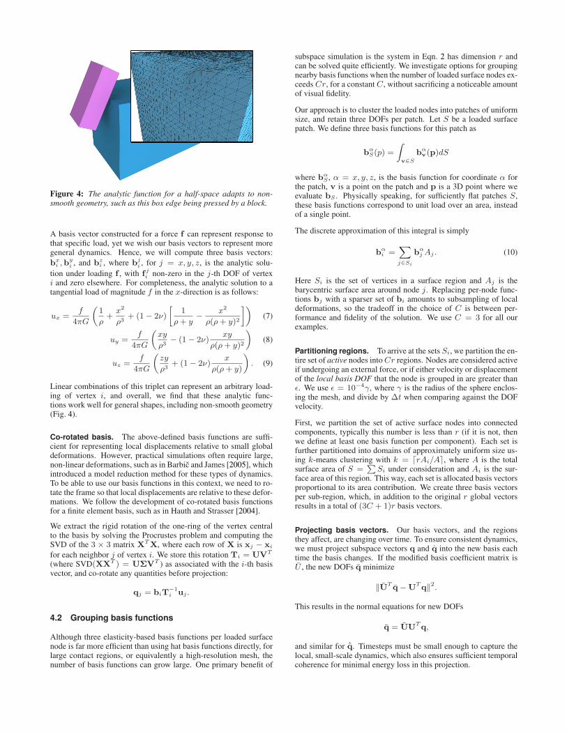
Figure 4: The analytic function for a half-space adapts to non-smooth geometry, such as this box edge being pressed by a block.

A basis vector constructed for a force f can represent response tothat specific load, yet we wish our basis vectors to represent moregeneral dynamics. Hence, we will compute three basis vectors:

bxi ,b

yi , and bz

i , where bji , for j = x, y, z, is the analytic solu-

tion under loading f , with fji non-zero in the j-th DOF of vertex

i and zero elsewhere. For completeness, the analytic solution to atangential load of magnitude f in the x-direction is as follows:

ux =f

4πG

(

1

ρ+

x2

ρ3+ (1− 2ν)

[

1

ρ+ y−

x2

ρ(ρ+ y)2

])

(7)

uy =f

4πG

(

xy

ρ3− (1− 2ν)

xy

ρ(ρ+ y)2

)

(8)

uz =f

4πG

(

zy

ρ3+ (1− 2ν)

x

ρ(ρ+ y)

)

. (9)

Linear combinations of this triplet can represent an arbitrary load-ing of vertex i, and overall, we find that these analytic func-tions work well for general shapes, including non-smooth geometry(Fig. 4).

Co-rotated basis. The above-defined basis functions are suffi-cient for representing local displacements relative to small globaldeformations. However, practical simulations often require large,non-linear deformations, such as in Barbic and James [2005], whichintroduced a model reduction method for these types of dynamics.To be able to use our basis functions in this context, we need to ro-tate the frame so that local displacements are relative to these defor-mations. We follow the development of co-rotated basis functionsfor a finite element basis, such as in Hauth and Strasser [2004].

We extract the rigid rotation of the one-ring of the vertex centralto the basis by solving the Procrustes problem and computing theSVD of the 3 × 3 matrix XTX, where each row of X is xj − xi

for each neighbor j of vertex i. We store this rotation Ti = UVT

(where SVD(XXT ) = UΣVT ) as associated with the i-th basisvector, and co-rotate any quantities before projection:

qj = biT−1

i uj .

4.2 Grouping basis functions

Although three elasticity-based basis functions per loaded surfacenode is far more efficient than using hat basis functions directly, forlarge contact regions, or equivalently a high-resolution mesh, thenumber of basis functions can grow large. One primary benefit of

subspace simulation is the system in Eqn. 2 has dimension r andcan be solved quite efficiently. We investigate options for groupingnearby basis functions when the number of loaded surface nodes ex-ceeds Cr, for a constant C, without sacrificing a noticeable amountof visual fidelity.

Our approach is to cluster the loaded nodes into patches of uniformsize, and retain three DOFs per patch. Let S be a loaded surfacepatch. We define three basis functions for this patch as

bαS(p) =

∫

v∈S

bαv(p)dS

where bαS , α = x, y, z, is the basis function for coordinate α for

the patch, v is a point on the patch and p is a 3D point where weevaluate bS . Physically speaking, for sufficiently flat patches S,these basis functions correspond to unit load over an area, insteadof a single point.

The discrete approximation of this integral is simply

bαi =

∑

j∈Si

bαj Aj . (10)

Here Si is the set of vertices in a surface region and Aj is thebarycentric surface area around node j. Replacing per-node func-tions bj with a sparser set of bi amounts to subsampling of localdeformations, so the tradeoff in the choice of C is between per-formance and fidelity of the solution. We use C = 3 for all ourexamples.

Partitioning regions. To arrive at the sets Si, we partition the en-tire set of active nodes into Cr regions. Nodes are considered activeif undergoing an external force, or if either velocity or displacementof the local basis DOF that the node is grouped in are greater thanǫ. We use ǫ = 10−4γ, where γ is the radius of the sphere enclos-ing the mesh, and divide by ∆t when comparing against the DOFvelocity.

First, we partition the set of active surface nodes into connectedcomponents, typically this number is less than r (if it is not, thenwe define at least one basis function per component). Each set isfurther partitioned into domains of approximately uniform size us-ing k-means clustering with k = ⌈rAi/A⌉, where A is the totalsurface area of S =

∑

Si under consideration and Ai is the sur-face area of this region. This way, each set is allocated basis vectorsproportional to its area contribution. We create three basis vectorsper sub-region, which, in addition to the original r global vectorsresults in a total of (3C + 1)r basis vectors.

Projecting basis vectors. Our basis vectors, and the regionsthey affect, are changing over time. To ensure consistent dynamics,we must project subspace vectors q and q into the new basis eachtime the basis changes. If the modified basis coefficient matrix isU , the new DOFs q minimize

‖UTq−U

Tq‖2.

This results in the normal equations for new DOFs

q = UUTq,

and similar for ˙q. Timesteps must be small enough to capture thelocal, small-scale dynamics, which also ensures sufficient temporalcoherence for minimal energy loss in this projection.

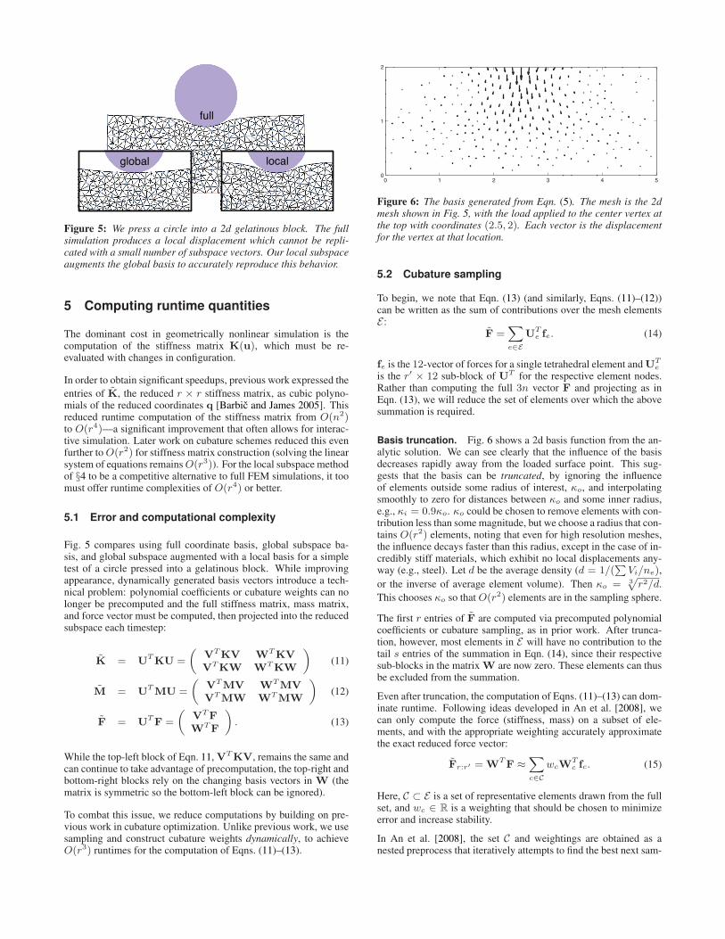
full

global local

Figure 5: We press a circle into a 2d gelatinous block. The fullsimulation produces a local displacement which cannot be repli-cated with a small number of subspace vectors. Our local subspaceaugments the global basis to accurately reproduce this behavior.

5 Computing runtime quantities

The dominant cost in geometrically nonlinear simulation is thecomputation of the stiffness matrix K(u), which must be re-evaluated with changes in configuration.

In order to obtain significant speedups, previous work expressed the

entries of K, the reduced r × r stiffness matrix, as cubic polyno-mials of the reduced coordinates q [Barbic and James 2005]. Thisreduced runtime computation of the stiffness matrix from O(n2)to O(r4)—a significant improvement that often allows for interac-tive simulation. Later work on cubature schemes reduced this evenfurther to O(r2) for stiffness matrix construction (solving the linearsystem of equations remains O(r3)). For the local subspace methodof §4 to be a competitive alternative to full FEM simulations, it toomust offer runtime complexities of O(r4) or better.

5.1 Error and computational complexity

Fig. 5 compares using full coordinate basis, global subspace ba-sis, and global subspace augmented with a local basis for a simpletest of a circle pressed into a gelatinous block. While improvingappearance, dynamically generated basis vectors introduce a tech-nical problem: polynomial coefficients or cubature weights can nolonger be precomputed and the full stiffness matrix, mass matrix,and force vector must be computed, then projected into the reducedsubspace each timestep:

K = UTKU =

(

VTKV WTKV

VTKW WTKW

)

(11)

M = UTMU =

(

VTMV WTMV

VTMW WTMW

)

(12)

F = UTF =

(

VTF

WTF

)

. (13)

While the top-left block of Eqn. 11, VTKV, remains the same andcan continue to take advantage of precomputation, the top-right andbottom-right blocks rely on the changing basis vectors in W (thematrix is symmetric so the bottom-left block can be ignored).

To combat this issue, we reduce computations by building on pre-vious work in cubature optimization. Unlike previous work, we usesampling and construct cubature weights dynamically, to achieveO(r3) runtimes for the computation of Eqns. (11)–(13).

0 1 2 3 4 50

1

2

Figure 6: The basis generated from Eqn. (5). The mesh is the 2dmesh shown in Fig. 5, with the load applied to the center vertex atthe top with coordinates (2.5, 2). Each vector is the displacementfor the vertex at that location.

5.2 Cubature sampling

To begin, we note that Eqn. (13) (and similarly, Eqns. (11)–(12))can be written as the sum of contributions over the mesh elementsE :

F =∑

e∈E

UTe fe. (14)

fe is the 12-vector of forces for a single tetrahedral element and UTe

is the r′ × 12 sub-block of UT for the respective element nodes.Rather than computing the full 3n vector F and projecting as inEqn. (13), we will reduce the set of elements over which the abovesummation is required.

Basis truncation. Fig. 6 shows a 2d basis function from the an-alytic solution. We can see clearly that the influence of the basisdecreases rapidly away from the loaded surface point. This sug-gests that the basis can be truncated, by ignoring the influenceof elements outside some radius of interest, κo, and interpolatingsmoothly to zero for distances between κo and some inner radius,e.g., κi = 0.9κo. κo could be chosen to remove elements with con-tribution less than some magnitude, but we choose a radius that con-tains O(r2) elements, noting that even for high resolution meshes,the influence decays faster than this radius, except in the case of in-credibly stiff materials, which exhibit no local displacements any-way (e.g., steel). Let d be the average density (d = 1/(

∑

Vi/ne),

or the inverse of average element volume). Then κo = 3√

r2/d.

This chooses κo so that O(r2) elements are in the sampling sphere.

The first r entries of F are computed via precomputed polynomialcoefficients or cubature sampling, as in prior work. After trunca-tion, however, most elements in E will have no contribution to thetail s entries of the summation in Eqn. (14), since their respectivesub-blocks in the matrix W are now zero. These elements can thusbe excluded from the summation.

Even after truncation, the computation of Eqns. (11)–(13) can dom-inate runtime. Following ideas developed in An et al. [2008], wecan only compute the force (stiffness, mass) on a subset of ele-ments, and with the appropriate weighting accurately approximatethe exact reduced force vector:

Fr:r′ = WTF ≈

∑

c∈C

wcWTc fc. (15)

Here, C ⊂ E is a set of representative elements drawn from the fullset, and wc ∈ R is a weighting that should be chosen to minimizeerror and increase stability.

In An et al. [2008], the set C and weightings are obtained as anested preprocess that iteratively attempts to find the best next sam-

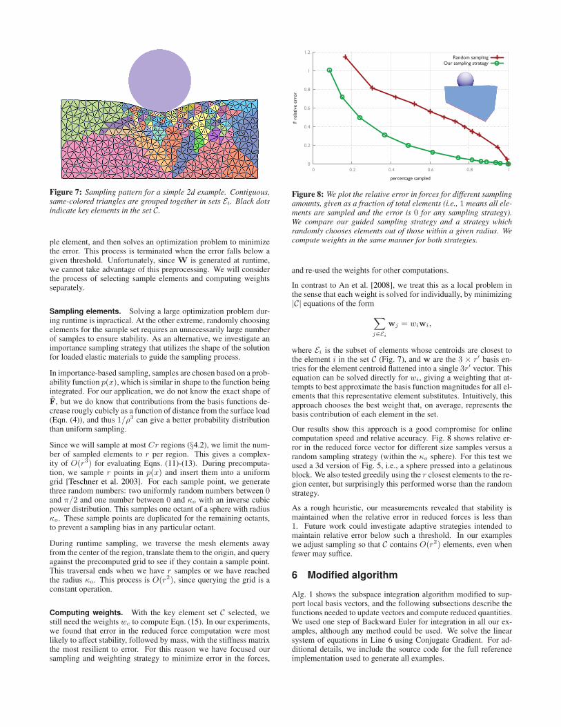
Figure 7: Sampling pattern for a simple 2d example. Contiguous,same-colored triangles are grouped together in sets Ei. Black dotsindicate key elements in the set C.

ple element, and then solves an optimization problem to minimizethe error. This process is terminated when the error falls below agiven threshold. Unfortunately, since W is generated at runtime,we cannot take advantage of this preprocessing. We will considerthe process of selecting sample elements and computing weightsseparately.

Sampling elements. Solving a large optimization problem dur-ing runtime is inpractical. At the other extreme, randomly choosingelements for the sample set requires an unnecessarily large numberof samples to ensure stability. As an alternative, we investigate animportance sampling strategy that utilizes the shape of the solutionfor loaded elastic materials to guide the sampling process.

In importance-based sampling, samples are chosen based on a prob-ability function p(x), which is similar in shape to the function beingintegrated. For our application, we do not know the exact shape of

F, but we do know that contributions from the basis functions de-crease rougly cubicly as a function of distance from the surface load(Eqn. (4)), and thus 1/ρ3 can give a better probability distributionthan uniform sampling.

Since we will sample at most Cr regions (§4.2), we limit the num-ber of sampled elements to r per region. This gives a complex-ity of O(r3) for evaluating Eqns. (11)-(13). During precomputa-tion, we sample r points in p(x) and insert them into a uniformgrid [Teschner et al. 2003]. For each sample point, we generatethree random numbers: two uniformly random numbers between 0and π/2 and one number between 0 and κo with an inverse cubicpower distribution. This samples one octant of a sphere with radiusκo. These sample points are duplicated for the remaining octants,to prevent a sampling bias in any particular octant.

During runtime sampling, we traverse the mesh elements awayfrom the center of the region, translate them to the origin, and queryagainst the precomputed grid to see if they contain a sample point.This traversal ends when we have r samples or we have reachedthe radius κo. This process is O(r2), since querying the grid is aconstant operation.

Computing weights. With the key element set C selected, westill need the weights wc to compute Eqn. (15). In our experiments,we found that error in the reduced force computation were mostlikely to affect stability, followed by mass, with the stiffness matrixthe most resilient to error. For this reason we have focused oursampling and weighting strategy to minimize error in the forces,

Figure 8: We plot the relative error in forces for different samplingamounts, given as a fraction of total elements (i.e., 1 means all ele-ments are sampled and the error is 0 for any sampling strategy).We compare our guided sampling strategy and a strategy whichrandomly chooses elements out of those within a given radius. Wecompute weights in the same manner for both strategies.

and re-used the weights for other computations.

In contrast to An et al. [2008], we treat this as a local problem inthe sense that each weight is solved for individually, by minimizing|C| equations of the form

∑

j∈Ei

wj = wiwi,

where Ei is the subset of elements whose centroids are closest tothe element i in the set C (Fig. 7), and w are the 3 × r′ basis en-tries for the element centroid flattened into a single 3r′ vector. Thisequation can be solved directly for wi, giving a weighting that at-tempts to best approximate the basis function magnitudes for all el-ements that this representative element substitutes. Intuitively, thisapproach chooses the best weight that, on average, represents thebasis contribution of each element in the set.

Our results show this approach is a good compromise for onlinecomputation speed and relative accuracy. Fig. 8 shows relative er-ror in the reduced force vector for different size samples versus arandom sampling strategy (within the κo sphere). For this test weused a 3d version of Fig. 5, i.e., a sphere pressed into a gelatinousblock. We also tested greedily using the r closest elements to the re-gion center, but surprisingly this performed worse than the randomstrategy.

As a rough heuristic, our measurements revealed that stability ismaintained when the relative error in reduced forces is less than1. Future work could investigate adaptive strategies intended tomaintain relative error below such a threshold. In our exampleswe adjust sampling so that C contains O(r2) elements, even whenfewer may suffice.

6 Modified algorithm

Alg. 1 shows the subspace integration algorithm modified to sup-port local basis vectors, and the following subsections describe thefunctions needed to update vectors and compute reduced quantities.We used one step of Backward Euler for integration in all our ex-amples, although any method could be used. We solve the linearsystem of equations in Line 6 using Conjugate Gradient. For ad-ditional details, we include the source code for the full referenceimplementation used to generate all examples.

Algorithm 1 Use Backward Euler integration to step subspace po-sitions and and velocities by time h = tn+1 − tn

1: STEP(qn, qn, h)2: q = qn + hqn

3: (Fext,L) = getSurfaceLoads(q) {§6.1}4: U = updateBasis(L) {§6.2}

5: (Fint, K, M) = computeReducedQuantities(q,U,L) {§6.3}

6: ∆qn+1 = −(M+ h2K)−1(Fint + Fext)h7: qn+1 = qn +∆qn+1

8: qn+1 = qn + qn+1

R

∆R qT ABS

δR ||q ||s

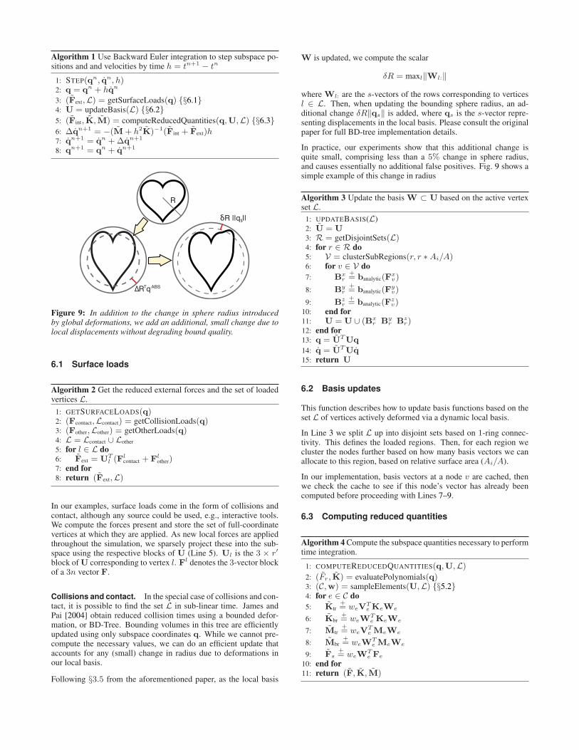
Figure 9: In addition to the change in sphere radius introducedby global deformations, we add an additional, small change due tolocal displacements without degrading bound quality.

6.1 Surface loads

Algorithm 2 Get the reduced external forces and the set of loadedvertices L.

1: GETSURFACELOADS(q)2: (Fcontact,Lcontact) = getCollisionLoads(q)3: (Fother,Lother) = getOtherLoads(q)4: L = Lcontact ∪ Lother

5: for l ∈ L do6: Fext = UT

l (Flcontact + Fl

other)7: end for8: return (Fext,L)

In our examples, surface loads come in the form of collisions andcontact, although any source could be used, e.g., interactive tools.We compute the forces present and store the set of full-coordinatevertices at which they are applied. As new local forces are appliedthroughout the simulation, we sparsely project these into the sub-space using the respective blocks of U (Line 5). Ul is the 3 × r′

block of U corresponding to vertex l. Fl denotes the 3-vector blockof a 3n vector F.

Collisions and contact. In the special case of collisions and con-tact, it is possible to find the set L in sub-linear time. James andPai [2004] obtain reduced collision times using a bounded defor-mation, or BD-Tree. Bounding volumes in this tree are efficientlyupdated using only subspace coordinates q. While we cannot pre-compute the necessary values, we can do an efficient update thataccounts for any (small) change in radius due to deformations inour local basis.

Following §3.5 from the aforementioned paper, as the local basis

W is updated, we compute the scalar

δR = maxl‖Wl:‖

where Wl: are the s-vectors of the rows corresponding to verticesl ∈ L. Then, when updating the bounding sphere radius, an ad-ditional change δR‖qs‖ is added, where qs is the s-vector repre-senting displacements in the local basis. Please consult the originalpaper for full BD-tree implementation details.

In practice, our experiments show that this additional change isquite small, comprising less than a 5% change in sphere radius,and causes essentially no additional false positives. Fig. 9 shows asimple example of this change in radius

Algorithm 3 Update the basis W ⊂ U based on the active vertexset L.

1: UPDATEBASIS(L)2: U = U3: R = getDisjointSets(L)4: for r ∈ R do5: V = clusterSubRegions(r, r ∗Ai/A)6: for v ∈ V do

7: Bxr

+= banalytic(F

xv)

8: Byr

+= banalytic(F

yv)

9: Bzr

+= banalytic(F

zv)

10: end for11: U = U ∪ (Bx

r Byr Bz

r)12: end for13: q = UTUq

14: q = UTUq15: return U

6.2 Basis updates

This function describes how to update basis functions based on theset L of vertices actively deformed via a dynamic local basis.

In Line 3 we split L up into disjoint sets based on 1-ring connec-tivity. This defines the loaded regions. Then, for each region wecluster the nodes further based on how many basis vectors we canallocate to this region, based on relative surface area (Ai/A).

In our implementation, basis vectors at a node v are cached, thenwe check the cache to see if this node’s vector has already beencomputed before proceeding with Lines 7–9.

6.3 Computing reduced quantities

Algorithm 4 Compute the subspace quantities necessary to performtime integration.

1: COMPUTEREDUCEDQUANTITIES(q,U,L)

2: (Fr, K) = evaluatePolynomials(q)3: (C,w) = sampleElements(U,L) {§5.2}4: for e ∈ C do

5: Ktr+= weV

Te KeWe

6: Kbr+= weW

Te KeWe

7: Mtr+= weV

Te MeWe

8: Mbr+= weW

Te MeWe

9: Fs+= weW

Te Fe

10: end for11: return (F, K, M)

In Alg. 4, the function evaluatePolynomials uses precomputeddata [Barbic and James 2005] or cubature optimization [An et al.

2008] to evaluate the first r sub-vector of F and the (r, r) top-left

sub-block of K. The subscripts tr and br denote the (r, s) top-rightand (s, s) bottom-right sub-blocks of the respective matrices.

7 Results

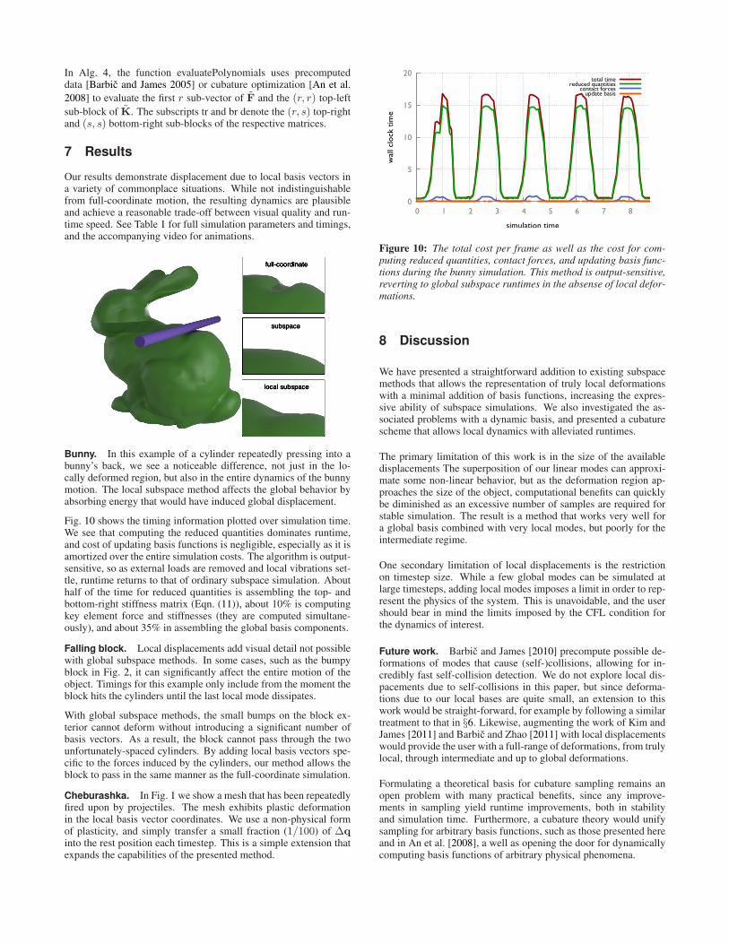
Our results demonstrate displacement due to local basis vectors ina variety of commonplace situations. While not indistinguishablefrom full-coordinate motion, the resulting dynamics are plausibleand achieve a reasonable trade-off between visual quality and run-time speed. See Table 1 for full simulation parameters and timings,and the accompanying video for animations.

Bunny. In this example of a cylinder repeatedly pressing into abunny’s back, we see a noticeable difference, not just in the lo-cally deformed region, but also in the entire dynamics of the bunnymotion. The local subspace method affects the global behavior byabsorbing energy that would have induced global displacement.

Fig. 10 shows the timing information plotted over simulation time.We see that computing the reduced quantities dominates runtime,and cost of updating basis functions is negligible, especially as it isamortized over the entire simulation costs. The algorithm is output-sensitive, so as external loads are removed and local vibrations set-tle, runtime returns to that of ordinary subspace simulation. Abouthalf of the time for reduced quantities is assembling the top- andbottom-right stiffness matrix (Eqn. (11)), about 10% is computingkey element force and stiffnesses (they are computed simultane-ously), and about 35% in assembling the global basis components.

Falling block. Local displacements add visual detail not possiblewith global subspace methods. In some cases, such as the bumpyblock in Fig. 2, it can significantly affect the entire motion of theobject. Timings for this example only include from the moment theblock hits the cylinders until the last local mode dissipates.

With global subspace methods, the small bumps on the block ex-terior cannot deform without introducing a significant number ofbasis vectors. As a result, the block cannot pass through the twounfortunately-spaced cylinders. By adding local basis vectors spe-cific to the forces induced by the cylinders, our method allows theblock to pass in the same manner as the full-coordinate simulation.

Cheburashka. In Fig. 1 we show a mesh that has been repeatedlyfired upon by projectiles. The mesh exhibits plastic deformationin the local basis vector coordinates. We use a non-physical formof plasticity, and simply transfer a small fraction (1/100) of ∆qinto the rest position each timestep. This is a simple extension thatexpands the capabilities of the presented method.

0

5

10

15

20

0 1 2 3 4 5 6 7 8

wal

l cl

ock

tim

e

simulation time

total timereduced quantities

contact forcesupdate basis

Figure 10: The total cost per frame as well as the cost for com-puting reduced quantities, contact forces, and updating basis func-tions during the bunny simulation. This method is output-sensitive,reverting to global subspace runtimes in the absense of local defor-mations.

8 Discussion

We have presented a straightforward addition to existing subspacemethods that allows the representation of truly local deformationswith a minimal addition of basis functions, increasing the expres-sive ability of subspace simulations. We also investigated the as-sociated problems with a dynamic basis, and presented a cubaturescheme that allows local dynamics with alleviated runtimes.

The primary limitation of this work is in the size of the availabledisplacements The superposition of our linear modes can approxi-mate some non-linear behavior, but as the deformation region ap-proaches the size of the object, computational benefits can quicklybe diminished as an excessive number of samples are required forstable simulation. The result is a method that works very well fora global basis combined with very local modes, but poorly for theintermediate regime.

One secondary limitation of local displacements is the restrictionon timestep size. While a few global modes can be simulated atlarge timesteps, adding local modes imposes a limit in order to rep-resent the physics of the system. This is unavoidable, and the usershould bear in mind the limits imposed by the CFL condition forthe dynamics of interest.

Future work. Barbic and James [2010] precompute possible de-formations of modes that cause (self-)collisions, allowing for in-credibly fast self-collision detection. We do not explore local dis-pacements due to self-collisions in this paper, but since deforma-tions due to our local bases are quite small, an extension to thiswork would be straight-forward, for example by following a similartreatment to that in §6. Likewise, augmenting the work of Kim andJames [2011] and Barbic and Zhao [2011] with local displacementswould provide the user with a full-range of deformations, from trulylocal, through intermediate and up to global deformations.

Formulating a theoretical basis for cubature sampling remains anopen problem with many practical benefits, since any improve-ments in sampling yield runtime improvements, both in stabilityand simulation time. Furthermore, a cubature theory would unifysampling for arbitrary basis functions, such as those presented hereand in An et al. [2008], a well as opening the door for dynamicallycomputing basis functions of arbitrary physical phenomena.

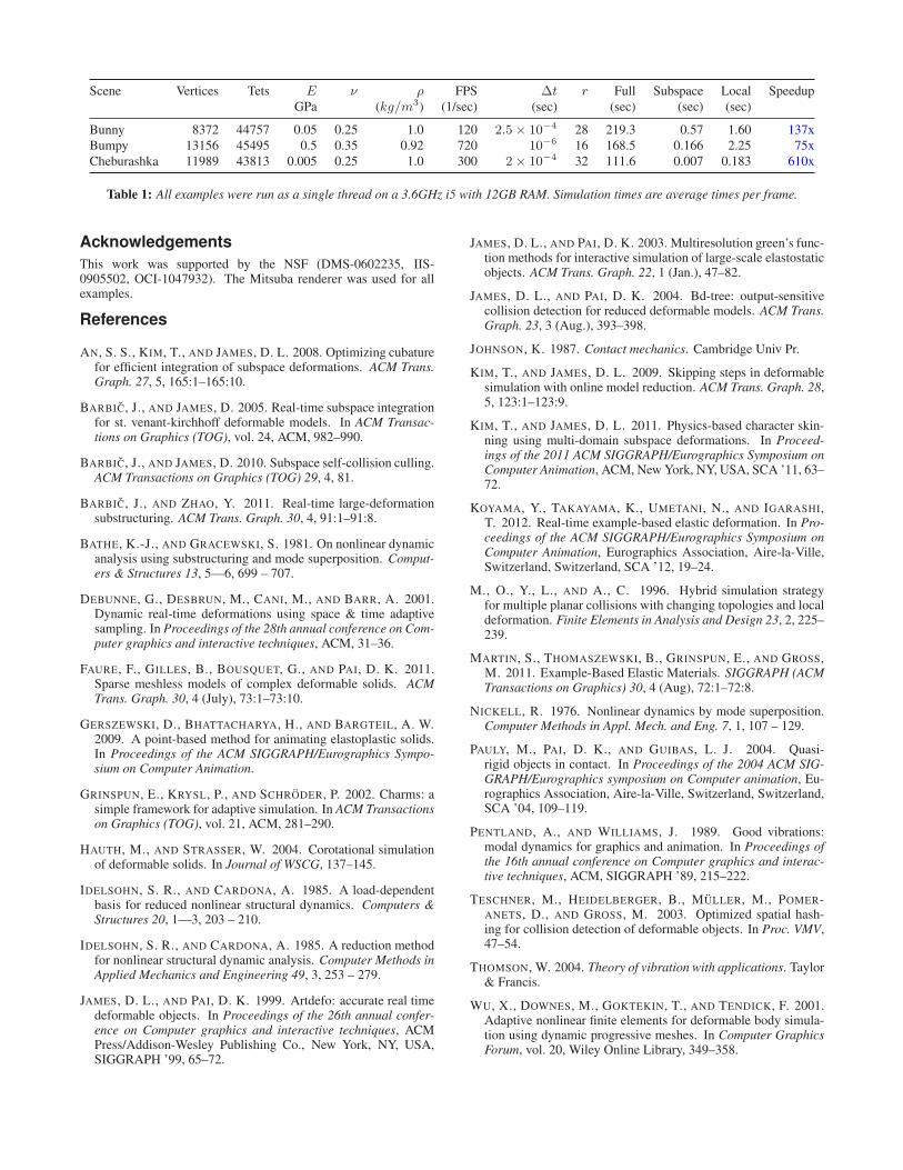
Scene Vertices Tets E ν ρ FPS ∆t r Full Subspace Local Speedup

GPa (kg/m3) (1/sec) (sec) (sec) (sec) (sec)

Bunny 8372 44757 0.05 0.25 1.0 120 2.5× 10−4 28 219.3 0.57 1.60 137x

Bumpy 13156 45495 0.5 0.35 0.92 720 10−6 16 168.5 0.166 2.25 75x

Cheburashka 11989 43813 0.005 0.25 1.0 300 2× 10−4 32 111.6 0.007 0.183 610x

Table 1: All examples were run as a single thread on a 3.6GHz i5 with 12GB RAM. Simulation times are average times per frame.

Acknowledgements

This work was supported by the NSF (DMS-0602235, IIS-0905502, OCI-1047932). The Mitsuba renderer was used for allexamples.

References

AN, S. S., KIM, T., AND JAMES, D. L. 2008. Optimizing cubaturefor efficient integration of subspace deformations. ACM Trans.Graph. 27, 5, 165:1–165:10.

BARBIC, J., AND JAMES, D. 2005. Real-time subspace integrationfor st. venant-kirchhoff deformable models. In ACM Transac-tions on Graphics (TOG), vol. 24, ACM, 982–990.

BARBIC, J., AND JAMES, D. 2010. Subspace self-collision culling.ACM Transactions on Graphics (TOG) 29, 4, 81.

BARBIC, J., AND ZHAO, Y. 2011. Real-time large-deformationsubstructuring. ACM Trans. Graph. 30, 4, 91:1–91:8.

BATHE, K.-J., AND GRACEWSKI, S. 1981. On nonlinear dynamicanalysis using substructuring and mode superposition. Comput-ers & Structures 13, 5—6, 699 – 707.

DEBUNNE, G., DESBRUN, M., CANI, M., AND BARR, A. 2001.Dynamic real-time deformations using space & time adaptivesampling. In Proceedings of the 28th annual conference on Com-puter graphics and interactive techniques, ACM, 31–36.

FAURE, F., GILLES, B., BOUSQUET, G., AND PAI, D. K. 2011.Sparse meshless models of complex deformable solids. ACMTrans. Graph. 30, 4 (July), 73:1–73:10.

GERSZEWSKI, D., BHATTACHARYA, H., AND BARGTEIL, A. W.2009. A point-based method for animating elastoplastic solids.In Proceedings of the ACM SIGGRAPH/Eurographics Sympo-sium on Computer Animation.

GRINSPUN, E., KRYSL, P., AND SCHRODER, P. 2002. Charms: asimple framework for adaptive simulation. In ACM Transactionson Graphics (TOG), vol. 21, ACM, 281–290.

HAUTH, M., AND STRASSER, W. 2004. Corotational simulationof deformable solids. In Journal of WSCG, 137–145.

IDELSOHN, S. R., AND CARDONA, A. 1985. A load-dependentbasis for reduced nonlinear structural dynamics. Computers &Structures 20, 1—3, 203 – 210.

IDELSOHN, S. R., AND CARDONA, A. 1985. A reduction methodfor nonlinear structural dynamic analysis. Computer Methods inApplied Mechanics and Engineering 49, 3, 253 – 279.

JAMES, D. L., AND PAI, D. K. 1999. Artdefo: accurate real timedeformable objects. In Proceedings of the 26th annual confer-ence on Computer graphics and interactive techniques, ACMPress/Addison-Wesley Publishing Co., New York, NY, USA,SIGGRAPH ’99, 65–72.

JAMES, D. L., AND PAI, D. K. 2003. Multiresolution green’s func-tion methods for interactive simulation of large-scale elastostaticobjects. ACM Trans. Graph. 22, 1 (Jan.), 47–82.

JAMES, D. L., AND PAI, D. K. 2004. Bd-tree: output-sensitivecollision detection for reduced deformable models. ACM Trans.Graph. 23, 3 (Aug.), 393–398.

JOHNSON, K. 1987. Contact mechanics. Cambridge Univ Pr.

KIM, T., AND JAMES, D. L. 2009. Skipping steps in deformablesimulation with online model reduction. ACM Trans. Graph. 28,5, 123:1–123:9.

KIM, T., AND JAMES, D. L. 2011. Physics-based character skin-ning using multi-domain subspace deformations. In Proceed-ings of the 2011 ACM SIGGRAPH/Eurographics Symposium onComputer Animation, ACM, New York, NY, USA, SCA ’11, 63–72.

KOYAMA, Y., TAKAYAMA, K., UMETANI, N., AND IGARASHI,T. 2012. Real-time example-based elastic deformation. In Pro-ceedings of the ACM SIGGRAPH/Eurographics Symposium onComputer Animation, Eurographics Association, Aire-la-Ville,Switzerland, Switzerland, SCA ’12, 19–24.

M., O., Y., L., AND A., C. 1996. Hybrid simulation strategyfor multiple planar collisions with changing topologies and localdeformation. Finite Elements in Analysis and Design 23, 2, 225–239.

MARTIN, S., THOMASZEWSKI, B., GRINSPUN, E., AND GROSS,M. 2011. Example-Based Elastic Materials. SIGGRAPH (ACMTransactions on Graphics) 30, 4 (Aug), 72:1–72:8.

NICKELL, R. 1976. Nonlinear dynamics by mode superposition.Computer Methods in Appl. Mech. and Eng. 7, 1, 107 – 129.

PAULY, M., PAI, D. K., AND GUIBAS, L. J. 2004. Quasi-rigid objects in contact. In Proceedings of the 2004 ACM SIG-GRAPH/Eurographics symposium on Computer animation, Eu-rographics Association, Aire-la-Ville, Switzerland, Switzerland,SCA ’04, 109–119.

PENTLAND, A., AND WILLIAMS, J. 1989. Good vibrations:modal dynamics for graphics and animation. In Proceedings ofthe 16th annual conference on Computer graphics and interac-tive techniques, ACM, SIGGRAPH ’89, 215–222.

TESCHNER, M., HEIDELBERGER, B., MULLER, M., POMER-ANETS, D., AND GROSS, M. 2003. Optimized spatial hash-ing for collision detection of deformable objects. In Proc. VMV,47–54.

THOMSON, W. 2004. Theory of vibration with applications. Taylor& Francis.

WU, X., DOWNES, M., GOKTEKIN, T., AND TENDICK, F. 2001.Adaptive nonlinear finite elements for deformable body simula-tion using dynamic progressive meshes. In Computer GraphicsForum, vol. 20, Wiley Online Library, 349–358.