SU PPLEMENTARY INFORMATION - media. · PDF fileeral non-line-of-sight imaging approaches. The...

Supplementary Methods

Equipment details The time-resolved detector is a PDM series single photon avalanche diode (SPAD) from Mi-

cro Photon Devices with a 100 µm⇥ 100 µm active area, a reported 27 ps timing jitter (100 kHz laser at 675 nm),

and 40.9 dark counts per second. Detection events are time stamped with 4 ps temporal resolution using a PicoHarp

300 Time-Correlated Single Photon Counting (TCSPC) module. The detected light is focused by a 75mm achro-

matic doublet (Thorlabs AC254-075-A-ML), and filtered using a laser line filter (Thorlabs FL670-10). The detec-

tion optics are co-axially aligned with an active light source using a polarized beamsplitter (Thorlabs PBS251).

The light source (ALPHALAS PICOPOWER-LD-670-50) consists of a 670 nm wavelength pulsed laser diode

with a reported pulse width of 30.6 ps at a 10MHz repetition rate and 0.11mW average power. A 2-axis scanning

galvonometer (Thorlabs GVS012) raster scans the illumination and detection spots across a wall located approx-

imately 2m from the system at an oblique angle. The measured jitter of the entire system is approximately 60 ps

without the laser line filter, and 200 ps with the filter on. We only use the filter for the outdoor experiments to

reduce ambient light. The increase in jitter is due to the fact that the spectral transmission properties of the filter

affect the temporal characteristics of the imaging system via the time-bandwidth product.16 An appropriate choice

of spectral line filter and pulsed laser could mitigate this effect.

Challenges with confocal scanning Unlike conventional approaches, a confocalized NLOS system exposes the

detector to direct reflections. This can be problematic, because the overwhelmingly bright contribution of direct

light reduces the SNR of the indirect signal in two ways. First, after detecting a photon, the SPAD sensor becomes

inactive for approximately 75 ns and ignores any photons that strike the detector for this period of time (commonly

referred to as the dead time of the device). If the contribution of direct light is too strong, this reduces the detection

probability of indirect photons. Second, approximately 0.1% of detected photon events produce a secondary event

due to an effect known as afterpulsing. The contribution of direct photons therefore increases the number of

spurious photons detected by the SPAD, further reducing the SNR of the indirect signal.

To avoid the negative effects of a strong direct signal, a time-gated SPAD could be used for detection to gate

out photons due to direct light.16 Given that our SPAD operates in free-running mode, we instead illuminate and

image two slightly different points on a wall to reduce the contribution of direct light. The distance between these

points should be sufficiently small so as to not affect the confocal image formation model.

System calibration The first calibration step involves aligning the detector and light source by adjusting the

position of the beamsplitter to maximize the photon count rate. When perfectly aligned, the strong direct signal

significantly reduces the number of indirect photons detected by the SPAD. Therefore, the second step involves

slightly adjusting the position of the beamsplitter to decrease the direct photon counts and increase the indirect

WWW.NATURE.COM/NATURE | 1

SUPPLEMENTARY INFORMATIONdoi:10.1038/nature25489

photon counts originating from a hidden retroreflector placed within the scene (e.g., the exit sign). The SPAD

detected between 0.29 and 1 million counts per second for all experiments (i.e., the number of detected events

ranged between 2.9% and 10% of the total number of pulses). For the final step, the system scans a 6 ⇥ 6 grid of

points on the wall and uses the time of arrival of direct photons and known galvanometer mirror angles to compute

the relative position and orientation of the wall relative to the system.

Acquisition procedure The system scans 64⇥64 equidistant points on a wall for indoor experiments, and 32⇥32points for the outdoor experiment. At a 10MHz repetition rate, the PicoHarp 300 returns unprocessed histograms

containing 25, 000 bins with a temporal resolution of 4 ps per bin. The acquired histograms are temporally aligned

such that the direct pulses appear at time t = 0. Histograms are then trimmed to either 2048 bins for indoor

experiments or 4096 bins for the outdoor experiment. The first 600 bins are set to 0 to remove the direct component.

The histograms are then downsampled by a factor of 4 to either 512 or 1024 bins before processing, where each bin

now has a temporal resolution of 16 ps. The acquisition time for each histogram is either 0.1 s or 1 s, as indicated

for each respective experiment.

Validating radiometric falloff To verify the radiometric intensity falloff in the proposed image formation model,

we measure the intensity of a small patch behind the wall while varying the distance between the NLOS patch

and the sampled wall. Figure 1 shows the intensity response for several different materials: a diffuse patch and

retroreflective patches of different grades (“engineering” grade and “diamond” grade). For the diffuse patch, mea-

surements (blue circles) closely match the predicted 1r

4 falloff (blue line), where r is the distance between patch

and wall. Similarly, the diamond grade retroreflective material (red circles) closely matches the predicted 1r

2 falloff

(red line). Lower-quality retroreflectors, such as the engineering grade retroreflective material or most retroreflec-

tive paints, exhibit a falloff that is somewhere between diffuse and perfectly retroreflective. The engineering grade

retroreflective material (green circles), for example, can be modeled by a falloff term of 1r

2.3 (green line).

Note that the intensity falloff only includes the propagation distance between the visible wall and the hidden

surface as well as the distance back along the same path. The additional travel distance between the laser/detector

and the wall is fixed, and does not affect the intensity falloff rate.

Image formation We briefly review the conventional NLOS formulation that models the indirect light transport

that occurs between two different points on a wall. Several simplifying assumptions are made in the derivation of

this image formation model (see below), resulting in an approximation of the physical light transport process. We

then introduce the confocal NLOS image formation model, followed by the light cone transform and a discretiza-

tion of the proposed model.


SUPPLEMENTARY INFORMATIONRESEARCHdoi:10.1038/nature25489

0 0.2 0.4 0.6 0.8 1distance (m)

2

4

6

8

10

dete

cted

eve

nts

x104

diffuseretroreflector (engineer grade)retroreflector (diamond grade)

0 0.2 0.4 0.6 0.8 1distance (m)

100

102

104

106

108

dete

cted

eve

nts

diffuseretroreflector (engineer grade)retroreflector (diamond grade)

a

b

Figure 1: (a) A linear plot and (b) a semi-logarithmic plot of the number of indirect photons detected as a function ofan object’s distance from the wall. The target objects are 5 cm⇥ 5 cm squares with different reflectance properties.The number of events is approximated by the function 1

r

4 for the diffuse object (blue line), 1r

2.3 for the engineergrade retroreflector (green line), and 1

r

2 for the diamond grade retroreflector (red line).

Conventional non-line-of-sight imaging

As illustrated in Figure 2, conventional NLOS imaging records a transient image14, 25–27 of a flat wall with a

time-resolved detector while sequentially illuminating points on the wall with an ultra-short laser pulse.14–19 The

geometry and albedo of the wall is assumed to be known or it can be scanned in a pre-processing step. Without

loss of generality, we model the wall as a reference plane at position z = 0. The recorded transient image ⌧ is

⌧ (x0, y0, t) =

ZZZ

⌦

1

r2l

r2⇢ (x, y, z)⇥ (5)

�

✓q(x0 � x)

2+ (y0 � y)

2+ z2 +

q(x

l

� x)2+ (y

l

� y)2+ z2 � tc

◆dx dy dz.

Here, ⇢ is the sought-after albedo of the hidden scene at each point in the three-dimensional half-space ⌦ satisfying

z > 0. The transient image is recorded while the light source illuminates position xl

, yl

on the wall with an ultra-

short pulse. This pulse is diffusely reflected off the wall and then scattered by the hidden scene back towards the

wall. The radiometric term 1/r2l

r2 models the square distance falloff using the distance rl

between xl

, yl

and some

hidden scene point x, y, z, as well as the distance r from that point to the sampled detector position on the wall

x0, y0. This equation can be discretized as ⌧ = A⇢ and solved with an iterative numerical approach that does not

require A to be directly inverted.

The conventional NLOS image formation model makes the following assumptions: there is only single scat-

tering behind the wall (i.e., no inter-reflections in the hidden scene parts), and there are no occlusions between

hidden scene parts. We also assume surfaces reflect light isotropically (i.e., the ratio of reflected radiance is inde-

pendent of both the incident light direction and outgoing view direction), in order to avoid the added complexity

of introducing Lambert’s cosine terms to model diffuse surface reflections.



Opt

ical

Set

upTi

me

Prof

ile

Pulsed Point Emitters

wall wall wall

light source light source

Conventional NLOS Confocal NLOSa b c

Figure 2: Illustration of time profiles incident on a wall from two scatterers that emit or reflect ultra-short pulsesof light. (a) The two points emit a single pulse at the same time. (b) Conventional NLOS imaging scans severalcombinations of light source positions x

l

, yl

and detector positions on the wall; here, this is illustrated for one lightsource position. (c) Confocal NLOS scans over the wall once with a co-located illuminator and detector. Note thatthe time profiles of the confocal setup are identical to those of point emitters after scaling the arrival times by afactor of two.

Confocal non-line-of-sight imaging

Instead of exhaustively scanning different combinations of light source positions xl

, yl

and detector positions

x0, y0 on the wall, confocal NLOS imaging is a sequential scanning approach where the light source and a single

detector are co-axial, or “confocalized”. Data recorded with a confocal NLOS setup thus represents a subset

of the samples required by conventional NLOS imaging. One of the primary benefits of the confocal setup is

that it is consistent with existing scanned LIDAR systems that often use avalanche photodiodes (APDs) or single

photon avalanche diodes (SPADs). The proposed signal processing approach to NLOS imaging may therefore be

compatible with many existing scanners.

Here, the transient image on the wall is given by

⌧ (x0, y0, t) =

ZZZ

⌦

1

r4⇢ (x, y, z) �

✓2

q(x0 � x)

2+ (y0 � y)

2+ z2 � tc

◆dx dy dz. (6)

This image formation model shares the same assumptions as Equation (5) (i.e., no multi-bounce transport, no

occlusions, and isotropic scattering).

Equation (6) is a laterally (i.e., in x and y) shift-invariant convolution. The convolution kernel is the surface of

a spatio-temporal 4D hypercone

x2 + y2 + z2 �✓tc

2

◆2

= 0. (7)

This formulation for light propagation is similar to Minkowski’s light cone used in special relativity,28 except that

it models a spherical wavefront propagating at half the speed of light.



Dirac delta identity

The image formation model of Equation (6) can be rewritten in a more convenient form by squaring and scaling

the arguments of the Dirac delta with the following identity:Z

⌦f(x) � (2kx0 � xk2 � tc) dx =

Z

⌦f(x) kx0 � xk2 � kx0 � xk22 �

✓tc

2

◆2!

dx (8)

where we denote x = (x, y, z) and x0 = (x0, y0, 0) for simplicity.

Proof The Dirac delta function can be expressed as the limit of a sequence of normalized functions30

�(x) = lim✏!0+

✏

(x) = lim✏!0+

1

✏⇣x✏

⌘. (9)

For example, the limit of a sequence of normalized hat functions (i.e., (x) = max(1� |x|, 0)) is the Dirac delta

function. The following uses this definition and a change of variables, ✏ = ✏0 42kx0�xk2+tc

, to derive Equation (8):Z

⌦f(x) � (2kx0 � xk2 � tc) dx =

Z

⌦f(x) lim

✏!0+

1

✏

✓2kx0 � xk2 � tc

✏

◆dx

=

Z

⌦f(x) lim

✏

0!0+

2kx0 � xk2 + tc

4✏0

✓4kx0 � xk22 � (tc)2

4✏0

◆dx

=

Z

⌦f(x)

✓2kx0 � xk2 + tc

4

◆lim

✏

0!0+

1

✏0

kx0 � xk22 �

�tc

2

�2

✏0

!dx

=

Z

⌦f(x)

✓2kx0 � xk2 + tc

4

◆�

kx0 � xk22 �

✓tc

2

◆2!

dx

=

Z

⌦f(x) kx0 � xk2 � kx0 � xk22 �

✓tc

2

◆2!

dx ⌅ (10)

Radiometric considerations

One of several interesting and unique properties of confocal NLOS imaging is that the distance function r is

directly related to the measured time-of-flight as

2

c

q(x0 � x)

2+ (y0 � y)

2+ z2

| {z }r

= t , r =tc

2. (11)

Therefore, the corresponding radiometric term, 1r

4 , can be pulled out of the triple integral of Equation (6). For

conventional NLOS imaging, we only know the combined distance rl

+ r = tc, but we cannot easily use this

information to replace the radiometric falloff term 1/�r2l

r2�

in Equation (5).

Another important property is that retroreflective materials can be modeled by replacing the radiometric falloff

term 1r

4 with 1r

2 , signifying a drastic increase in the indirect light signal as a function of distance r. Retroreflective

materials cannot be handled appropriately by existing non-confocal NLOS methods.



The light cone transform

We propose the light cone transform (LCT) that expresses the confocal NLOS image formation model as a

shift-invariant 3D convolution in the transform domain. The LCT is a computationally efficient way for computing

the forward model and, more importantly, leads to a closed-form expression for the inverse problem.

We start by using the Dirac delta identity from Equation (8) to rewrite the image formation model in Equa-

tion (6) as

⌧ (x0, y0, t) =

ZZZ

⌦

1

r3⇢ (x, y, z) �

(x0 � x)

2+ (y0 � y)

2+ z2 �

✓tc

2

◆2!

dx dy dz. (12)

Next, we pull out the radiometric term from the integral and perform a change of variables by letting z =pu,

dz

du

= 12pu

such that

⌧ (x0, y0, t) =

✓2

tc

◆3 ZZZ

⌦⇢�x, y,pu��

(x0 � x)

2+ (y0 � y)

2+ u�

✓tc

2

◆2!

1

2pu

dx dy du. (13)

We also introduce a second change of variables using v =�tc

2

�2, such that

v32 ⌧

✓x0, y0,

2

c

pv

◆

| {z }R

t

{⌧}(x0,y

0,v)

=

ZZZ

⌦

1

2pu

⇢�x, y,pu�

| {z }R

z

{⇢}(x,y,u)

�⇣(x0 � x)

2+ (y0 � y)

2+ u� v

⌘

| {z }h(x0�x,y

0�y,v�u)

dx dy du. (14)

The image formation model is a 3D convolution, which can alternatively be written as

Rt

{⌧} = h ⇤Rz

{⇢} , (15)

where ⇤ is the 3D convolution operator, h is the shift-invariant convolution kernel, Rz

{·} resamples ⇢ along the

z-axis and attenuates the result by 1/2pu, and R

t

{·} resamples ⌧ along the time axis and scales the result by

v32 . Note that a similar transform is not known to exist for the conventional NLOS problem, and that the LCT is

specific to the confocal case.

Discretizing the image formation

The transforms introduced with the continuous image formation model (Equation (15)) are implemented as

discrete operations in practice. For example, the operation Rt

{⌧} can be represented as an integral transform

Rt

{⌧} (x0, y0, v) = v32 ⌧

✓x0, y0,

2

c

pv

◆=

Z

t>0v

32 �

✓t� 2

c

pv

◆⌧(x0, y0, t) dt . (16)

Note that this transformation applies to all points (x0, y0) independently.

The discrete analog of this transform is given by a matrix-vector multiplication Rt

⌧ , between the vectorized

representation of the transient image ⌧ 2 Rn

x

n

y

n

t

+ and matrix Rt

2 Rn

x

n

y

n

h

⇥n

x

n

y

n

t

+ . Consider the case of a



single measurement on the wall (i.e., nx

= 1 and ny

= 1), where ⌦xy

is the region sampled by the detector. The

individual elements of the vectorized transient image and corresponding transform matrix are then given by

(⌧ )j

=

ZZ

⌦xy

Zt

j

t

j�1

⌧(x0, y0, t) dt dx0 dy0 , (Rt

)ij

=

Zh

i

h

i�1

Zt

j

t

j�1

v32 �

✓t� 2

c

pv

◆dt dv , (17)

where 1 i nh

and 1 j nt

. Here, the transient image is defined over a range of time values [a, b] ⇢ (0,1),

which is uniformly discretized into nt

equal spaces such that a = t0 < t1 < · · · < tn

t

= b. Similarly, the matrix

Rt

resamples the transient image into nh

elements where�ca

2

�2= h0 < h1 < · · · < h

n

h

=�cb

2

�2.

The corresponding discrete analog of the transformation Rz

{⇢} is similarly defined as a matrix-vector prod-

uct Rz

⇢, between the vectorized representation of unknown surface albedos ⇢ 2 Rn

x

n

y

n

z

+ and matrix Rz

2Rn

x

n

y

n

h

⇥n

x

n

y

n

z

+ . The elements are defined as

(⇢)k

=

ZZ

⌦xy

Zz

k

z

k�1

⇢(x, y, z) dz dx dy , (Rz

)ik

=

Zh

i

h

i�1

Zz

k

z

k�1

1

2pu

��z �pu� dz du , (18)

where 1 k nz

and ca

2 = z0 < z1 < · · · < zn

z

= cb

2 .

The full discrete image formation model is therefore

⌧ = A⇢ = R�1t

HRz

⇢ . (19)

where the matrix A = R�1t

HRz

is referred to as the light transport matrix. Note that each of these matrices

is independently applied to the respective dimension and can therefore be applied to large-scale datasets in a

memory efficient way. The matrix H 2 Rn

x

n

y

n

h

⇥n

x

n

y

n

h

+ represents the shift-invariant 3D convolution with the

4D hypercone (i.e., a convolution with a discretized version of the kernel h), which models light transport in free

space in the transform domain. Together, these matrices represent the discrete light cone transform.

The discrete light cone transform provides a fast and memory efficient approach to computing both forward

light transport (i.e., A⇢) and inverse light transport (i.e., A�1⇢) without forming any of the matrices explicitly.

Computational efficiency is largely achieved using the convolution theorem to compute matrix-vector multiplica-

tions with H as element-wise multiplications in the Fourier domain. Similarly, matrix-vector multiplications with

their inverses are computed as element-wise divisions in the Fourier domain.

Inverse methods Here, we derive a closed-form solution for the discrete NLOS problem. We first assume that

the noise model associated with the discrete light transform model in Equation (19) satisfies

⌧̃ = H⇢̃+ ⌘, (20)

where ⌧̃ = Rt

⌧ , ⇢̃ = Rz

⇢, and ⌘ 2 Rn

x

n

y

n

h is white noise.



The solution ⇢̃⇤ that minimizes the mean square error with respect to the ground truth solution ⇢̃ is well known

to be given by the Wiener deconvolution filter:29

⇢̃⇤ = F�1

"1

bH· | bH|2| bH|2 + 1

↵

#F⌧̃ , (21)

where the matrix F represents the 3D discrete Fourier transform and bH is a diagonal matrix containing the Fourier

transform of the shift-invariant 3D convolution kernel. ↵ is a frequency-dependent term representing the signal-to-

noise ratio (SNR).

Expanding Equation (21) results in the closed-form solution for the confocal NLOS problem:

⇢⇤ = R�1z

F�1

"1

bH· | bH|2| bH|2 + 1

↵

#FR

t

⌧ . (22)

In the Supplementary Derivations, we also outline a maximum a posteriori estimator for the reconstruction problem

that lifts these assumptions on the noise model and that also allows image priors to be imposed on the reconstructed

volume.



Supplementary Discussion

Resolution limits The accuracy of the reconstructed shape depends on several factors, including the system jitter,

the scanning area 2w ⇥ 2w, and the distance of the hidden object from the wall z (Figure 3). Here, the resolution

limit is defined as the minimum resolvable distance of two scatterers �d. Specifically, two scattering points, q1

and q2, are resolvable in space only if their indirect signals are resolvable in time:

�d = abs (kp� q1k2 � kp� q2k2) �c�t

2(23)

Using this formula, a bound on the minimum axial distance, i.e., along the z-axis, can be defined as �z � c�t/2.

In practice, this bound is related to the full width at half maximum (FWHM) of the temporal jitter of the detection

system, represented by the scalar �, as

�z � c�

2(24)

As illustrated in Figure 3, the FWHM is a practical means to derive resolution limits of a NLOS imaging system

and it is closely related to diffraction-limited resolution limits in microscopy. Alternative resolution criteria include

the Rayleigh criterion and the Sparrow limit. However, due to the fact that the temporal point spread functions

in NLOS imaging are not Airy disks, the FWHM criterion is an appropriate formulation for this application. If

the temporal jitter follows a Gaussian shape, the FWHM is directly proportional to the standard deviation � of the

jitter as � = 2p2ln2�.

Similarly, we can derive an approximate bound on the lateral resolution �x. For this purpose, we assume that

�x is much smaller than the area of the wall being sampled, such that cos(✓) ⇡ c�t/ (2�x) (see Figure 3(d)).

norm

aliz

ed re

spon

se

wall wall

a b c

d

Figure 3: (a) Illustration of the temporal response of two hidden points measured at one location on a visiblesurface. Assuming that the jitter of the detection system is well-described by a Gaussian function, the differencein time of arrival �t of the response of two points has to be farther apart than the FWHM � of the Gaussian jitter,i.e., �t � �. Panel (a) illustrates the case where �t = �, which we consider the minimum resolvable difference.To derive bounds on (b) axial and (c, d) lateral resolvable feature size, �t is related to the axial (�z) and lateral(�x) difference in position of the two points q1/2. In this illustration, p indicates the scanned point on the visiblewall that carries the most amount of information for resolving the difference between the hidden points q1/2. Asshown in panels (c) and (d), the lateral resolution is mainly determined by the size of the sampled wall 2w and thedistance of the point to the wall z.



Then,

c�t

2⇡ �x cos(✓) ⇡ �x cos

⇣tan�1

⇣ z

w

⌘⌘(25)

= �xwp

w2 + z2(26)

Using the FWHM criterion, the minimum lateral distance between two points is

�x � cpw2 + z2

2w� (27)

The formulation above allows us to make several important insights. First, the smallest resolvable axial feature

size �z represents the lowest resolution bound for all NLOS imaging applications. Second, the smallest resolvable

lateral feature size �x is depth dependent and only in the limit of z = 0 equal to �z. For sufficiently large depth

values, i.e., z � w, �x increases linearly with z.

Note that these bounds not only apply to the confocal NLOS acquisition setup introduced in this paper, but

also to all conventional NLOS approaches that scan different combinations of imaged and illuminated positions on

the wall. The fundamental limit of resolvable feature size is dictated by the temporal resolution of the detection

system and the size of the sampled area on the wall, which is also noted in prior work.16 These insights are not

surprising, because they directly relate to characteristics of diffraction-limited, coherent imaging systems, where

resolution is governed by wavelength and numerical aperture.

We verify these theoretical bounds with two experiments using a planar resolution chart and a set of individual

reflectors. Both targets are custom-made from retroreflective material and shown in Figure 4 (left column). For

both experiments, the confocal laser scanner samples the wall at 64 ⇥ 64 uniformly-spaced locations over a total

area of 2w ⇥ 2w = 40 cm ⇥ 40 cm. The acquisition time per sampled location is constant (approx. 0.1 s) for all

experiments. The temporal uncertainty of the imaging system is 60 ps, including SPAD jitter and finite laser pulse

width. Using Equation (27), we predict lateral resolutions of approx. 2 cm and 3.1 cm when the NLOS target is

z = 40 cm and z = 65 cm away from the wall, respectively.

The resolution chart consists of 5 groups of lines, and the width of the lines in each group is 3 cm, 2 cm, 1.5 cm,

1 cm, and 0.5 cm. Based on our prediction, the first group should be just resolvable at a distance of z = 65 cm

and the second group should be just resolvable at z = 40 cm. Columns 2-5 of Figure 4 show maximum intensity

projections of reconstructed volumes via front and side views at two different target distances. As predicted,

group 1 is resolvable at the farther distance while moving the target closer to the wall allows for group 2 to be

recovered as well.

The second experiment shows a different resolution target that consists of 3 ⇥ 3 circular retroreflectors, each

with a diameter of 3.2 cm, spaced apart by 10 cm. As we move this target away from the wall, the resolution of the

reconstructed target slightly degrades and it becomes more noisy due to the deceased signal-to-noise ratio in the

measurements.



1

2 3

4

5

10 cm 10cm 10cm 10cm 10cm

10cm 10cm 10cm 10cm 10cm

target object front (z = 40 cm) side (z = 40 cm) front (z = 65 cm) side (z = 65 cm)

Figure 4: Experimental resolution analysis of confocal NLOS imaging. For this setup, the theoretical lateralresolution is �x ⇡ 2.0 cm for a plane at depth z = 40 cm, and �x ⇡ 3.1 cm at depth z = 65 cm. Images sharethe same scale. Row 1: This resolution chart has multiple groups of lines. According to the theoretical predictions,group 1 should be just resolvable at z = 65 cm and group 2 at z = 40 cm, which is observed in practice. Row 2:The lateral resolution of a set of circular reflectors degrades slightly as the target moves away from the wall.Moreover, the signal-to-noise ratio of the measurements decreases and results in noisier reconstructions at fartherdistances.

Compute time and memory requirements Here, we list expected runtimes and memory requirements for sev-

eral non-line-of-sight imaging approaches. The backprojection algorithm, a direct inverse of the light transport

matrix, and iterative approaches to solving the inverse problem have been proposed in previous work. The discrete

light cone transform introduced in this paper allows a direct inverse of the light transport matrix to be computed

with orders of magnitude lower computational complexity and less memory requirements than existing methods.

In the following, we assume for simplicity that the recorded histograms sample the hidden volume of resolution

N⇥N⇥N at N⇥N locations on the wall. Each of the measured locations is represented as a temporal histogram

of length N . Thus, the light transport matrix A is of size N3 ⇥ N3 and it contains N5 non-zero elements that

would have to be stored in a sparse matrix representation.

The backprojection algorithm is a matrix-vector product of the transpose light transport matrix and the measure-

ment vector, which has a computational complexity of O�N5�. The backprojection algorithm can be computed

without explicitly constructing the matrix, and only requires O�N3�

memory.

Computing the inverse light transport matrix, for example via the singular value decomposition, includes

O�N9�

computational complexity for computing the SVD as well as two additional matrix-vector multiplica-

tions and a vector-vector multiplication. The overall runtime is still on the order of O�N9�

and the memory

requirements just for storing the decompositions is O�N6�. An attractive alternative to the SVD would be an

iterative, large scale solver, such as the conjugate gradient method. In this case, the computational complexity for



each iteration would be in the same order as the backprojection algorithm. In practice, it is computationally more

efficient to discretize the light transport matrix for use in iterative inverse procedures,20 at the cost of increasing

memory requirements to the order of O�N5�.

The discrete light cone transform (LCT) applies a transformation operation along the time axis (O�N3�),

followed by a 3D Fourier transform (O�N3logN

�), an element-wise multiplication (O

�N3�), an inverse 3D

Fourier transform (O�N3logN

�), and another transformation operation (O

�N3�). The combined computational

complexity is O�N3logN

�. The alternating-direction method of multipliers (ADMM) and its linearized version

(L-ADMM) are iterative algorithms that apply the LCT sequentially along with other, computationally less com-

plex, proximal operators (see Supplementary Derivations). Therefore, the order of the computational complexity

per iteration is similar to that of the LCT. The LCT only requires a single volume to be stored in memory, so

the memory requirements are several orders of magnitude better than existing methods. ADMM and L-ADMM

require several intermediate variables of the same size as the volume to be stored but the order of memory required

remains the same as the LCT.

Backprojection Direct Iterative Direct Inverse ADMM L-ADMMInverse Inverse⇤ with LCT with LCT⇤ with LCT⇤

Runtime O�N5�

O�N9�

O�N5�

O�N3logN

�O�N3logN

�O�N3logN

�

Memory O�N3�

O�N6�

O�N5�

O�N3�

O�N3�

O�N3�

⇤ The complexity listed for iterative methods represent the computation and memory requirements per iteration.



Supplementary Results

In support of the results shown in the primary text, we show several additional results of C-NLOS imaging in

Figures 5–12. Here, Figures 5–9 are physical experiments. Figures 10–12 are simulations that explore the impact

of tradeoffs necessary to achieve lower acquisition times by either reducing exposure time or by subsampling the

wall.

Figure 5 shows a scene with a flat retroreflective traffic sign. The volume of recorded measurements is shown on

the upper left and other columns in the first row show two x� t slices of the measurements as indicated by dashed,

yellow lines. These represent only indirect parts of the recorded light transport; the direct reflections off the wall

are digitally gated out by the proposed acquisition procedure. Compared with a reconstruction via backprojection

(left column) or filtered backprojection (center left column), the proposed LCT-based reconstruction (center right

column) reveals significantly more details, making the text and arrow legible. Even with the Laplacian filter

proposed by Velten et al.15 (center left column), the filtered backprojection method is not able to adequately recover

the hidden scene, because the solution to the inverse system is only approximated but not actually computed.

Note that for conciseness, we have thus far assumed that the volume of unknown albedos is reconstructed

directly from the transient image captured of the visible wall. In practice, however, the histograms measured by

SPADs are not necessarily the same as the transient image. A single photon that hits a SPAD has some probability

of creating an electron avalanche that is then time-stamped by the time-to-digital converter. After a detected event,

the SPAD must be quenched before another event can be recorded. Assuming that the length of the emitted laser

pulse is significantly smaller than the SPAD’s dead time, at most one of the photons in that pulse can trigger an

event, which is not necessarily the first arriving photon. The presence or absence of a detected event within a

short window is thus a Bernoulli trial, which is repeated many times to accumulate the histogram. A sequence of

Bernoulli trials with constant probabilities results in measured histograms being observations of an inhomogeneous

Poisson process. In the Supplementary Derivations (next section), we develop a comprehensive signal processing

framework that incorporates Poisson noise in the measurements as well as scene priors on the recovered volume

of albedos. At the core of this signal processing framework is the light cone transform, but it is embedded in an

iterative optimization framework. Please refer to prior work for more details on the connection between transient

images and measured SPAD histograms.27

We show results of this iterative approach in the right column of Figure 5 and impose priors on the Poissonian

nature of the measurements, a nonnegativity prior on the recovered albedos, as well as a combination of sparsity

and isotropic 3D total variation (TV) priors on the albedos. Related priors are commonly applied in various

computational imaging applications, such as LIDAR,23 and they have also been proposed for NLOS imaging.17, 20

We are the first to develop appropriate formulations for incorporating these priors in NLOS applications that are

dominated by Poisson noise. Please refer to the mathematical derivations section for more details.



In Figure 6, we show another scene that contains two retroreflective objects that partly occlude each other.

Even though this scene violates one of the assumptions made by our image formation model, the reconstructions

in this experiment are relatively robust to these occlusions. The two characters are well-separated, as seen in the

x � z slices in the bottom row, and a small amount of residual blur in the LCT results (center right column) is

removed by adding a combination of sparsity and isotropic 3D TV priors to the unknown volume (right column).

Figure 7 shows another, more complex 3D scene. The front of the mannequin torso, head, and limbs are coated

with a retroreflective paint before recording this object. The 3D structure of this hidden scene is well-recovered.

Similar to Figures 5 and 6, the LCT reconstruction shows significant improvements over backprojection-type

approaches. Adding additional priors further improves our results.

A purely diffuse scene is tested in Figure 8. The SNR for diffuse NLOS scenes is significantly lower than

that of retroreflective scenes, as seen in the noisy measurements (top row). The decreased SNR results in much

noisier measurements for the LCT (center right column). Again, these can be mitigated by applying priors on the

recovered albedos, here promoting contiguous surfaces, but the overall reconstruction quality is slightly lower than

for retroreflective objects.

A scene captured outdoors in indirect sunlight is shown in Figure 9. The reconstructed retroreflective letter is

identifiable in the reconstruction despite the high levels of ambient sunlight. The letter is placed 115 cm away from

the wall. The wall itself consists of a light and dark stone, and so there is an observable variation in the intensity

of the measurements. The reconstruction method is robust in this challenging scenario.

All physical experiments, except for the “Outside S”, are recorded by sampling the wall at 64 ⇥ 64 locations

with 512 time bins for the temporal histograms, each with a precision of 16 ps. The “Outside S” scene is sampled at

32⇥32 locations on the wall. The exposure time per sample is 0.1 s for the “Exit Sign”, the “SU”, the “Outside S”

and the resolution chart scenes. The exposure time for the “Mannequin” and “Diffuse S” scenes is 1 s per sampled

location. Thus, the total exposure time therefore ranges from 1.7min for the “Outside S” scene and 68min for

the “Diffuse S” scene. The sampled area on the wall is 80 cm ⇥ 80 cm for the “Exit Sign”, 70 cm ⇥ 70 cm for

the “SU”, the “Mannequin”, and the “Diffuse S”, 1m ⇥ 1m for the “Outside S”, and 40 cm ⇥ 40 cm for the

resolution chart. The simulations in Figures 10 & 11 have a resolution of 512⇥512 spatial samples, and Figure 12

has a resolution of 256 ⇥ 256. Reconstruction times with the LCT approach are below 1 s for all scenes with a

resolution up to 64 ⇥ 64 samples and approx. 3–5min for the simulations with a resolution of 512 ⇥ 512. Our

unoptimized implementation of the backprojection method and the filtered backprojection methods took 8.5min

for the scenes with 64 ⇥ 64 samples, which makes our LCT-based reconstruction more than 500⇥ faster than the

inferior backprojection-type methods. Higher-resolution reconstructions with priors took significantly longer, up

to 8 hours for the simulations with a resolution of 512⇥ 512. See Table 1 for a summary of experimental details,

including the detected photon count for each experiment.



Me

asu

re

me

nts

x0 t

y0

30 cm

t

x0

30 cm

Backprojection

x

y

z

Filtered Backprojection

LCT

LCT +R+ + k·k1,TV

30 cm

y

x

30 cm 30cm 30cm

30cm

z

x

30 cm 30cm 30cm

Figure 5: Experimental result: “Exit Sign”. A planar, retroreflective traffic sign is imaged outside the direct line ofthe sight of the detector and light source. The volume of time-resolved measurements is shown in the top row alongwith two x � t slices or “streak images” indicated by dashed, yellow lines and a photograph of the traffic sign.Backprojection-type methods (left and center left columns) fail to recover fine details and are usually blob-like.The light cone transform (LCT) developed in this paper is a direct inverse method that unlocks significantly fasterand higher-quality reconstructions with a smaller memory footprint than other methods (center right column). TheLCT also allows for additional priors, such as nonnegativity, sparsity, or total variation, to be imposed on theunknown albedos (right column).



Me

asu

re

me

nts

x0 t

y0

20 cm

t

x0

20 cm

Backprojection

x

y

z


LCT

LCT +R+ + k·k1,TV

20 cm

y

x

20 cm 20cm 20cm

20cm

z

x

20 cm 20cm 20cm

Figure 6: Experimental result: “SU”. This scene contains two planar, retroreflective objects that partly occlude eachother. Even though occlusions violate one of the assumptions of the proposed image formation, the reconstructionsare relatively insensitive to this violation. Again, backprojection-type methods (left and center left columns) failto recover fine details whereas a direct inverse via the LCT (center right column) or via the LCT and scene priors(right column) allows for significantly better and also faster reconstructions.



Me

asu

re

me

nts

x0 t

y0

20 cm

t

x0

20 cm

Backprojection

x

y

z


LCT

LCT +R+ + k·k1,TV

20 cm

y

x

20 cm 20cm 20cm

20cm

z

x

20 cm 20cm 20cm

Figure 7: Experimental result: “Mannequin”. This scene has a more complex 3D structure than the planar objectsshown so far. The mannequin is coated with retroreflective paint. Despite its complex 3D structure, the man-nequin is composed of surface patches that are spatially well-separated from each other. The hands, arms, legs,head, and torso do not contain fine geometric detail and have sufficient spacing between them for backprojection-type reconstruction approaches (left and center left columns) to generate a reasonable approximation of the 3Dshape. Nevertheless, as with the previous examples, LCT-type reconstructions (center right and right columns) aresuccessful in recovering more details of the mannequin.



Me

asu

re

me

nts

x0 t

y0

20 cm

t

x0

20 cm

Backprojection

x

y

z


LCT

LCT +R+ + k·k1,TV

20 cm

y

x

20 cm 20cm 20cm

20cm

z

x

20 cm 20cm 20cm

Figure 8: Experimental result: “Diffuse S”. As opposed to the previous examples, this scene shows a planardiffuse object. Even with an exposure time of 1 second per sampled location, the measurements of this diffusescene (top row) are significantly noisier than those of retroreflective scenes because the intensity reduces withdistance at a faster rate for diffuse objects than for retroreflective objects. The noisy measurements propagate intothe reconstructions (center right column), but can be mitigated by a total variation (TV) prior (right column).



Me

asu

re

me

nts

x0 t

y0

30 cm

t

x0

30 cm

Backprojection

x

y

z


LCT

LCT +R+ + k·k1,TV

30 cm

y

x

30 cm 30cm 30cm

30cm

z

x

30 cm 30cm 30cm

Figure 9: Experimental result: “Outside S”. A planar, retroreflective object is imaged outdoors in indirect sunlight.The object is placed outside the direct line of sight of the detector, and approximately 115 cm away from a buildingwall. The wall is composed of light and dark-colored stone, and so measurements captured on the darker stone arenoticeably lower in intensity. Despite the challenging nature of the outdoor environment, the reconstructed letter isrecognizable in the LCT reconstruction (center right column), where details are more accurately represented thanwith filtered backprojection. Adding priors to the reconstruction further improves the quality of the reconstructedresult (right column).



Experiment name Samples Bins Detection area Exposure Retro. Counts1 Counts2 Counts3

Res. Chart (40 cm) 64⇥ 64 512 0.4m⇥ 0.4m 0.1 s Yes 1.0⇥ 105 5.9⇥ 104 2.9⇥ 103

Res. Chart (65 cm) 64⇥ 64 512 0.4m⇥ 0.4m 0.1 s Yes 1.0⇥ 105 5.5⇥ 104 1.8⇥ 103

Dot Chart (40 cm) 64⇥ 64 512 0.4m⇥ 0.4m 0.1 s Yes 1.0⇥ 105 5.8⇥ 104 1.4⇥ 103

Dot Chart (65 cm) 64⇥ 64 512 0.4m⇥ 0.4m 0.1 s Yes 1.0⇥ 105 5.9⇥ 104 0.8⇥ 103

Exit Sign 64⇥ 64 512 0.8m⇥ 0.8m 0.1 s Yes 4.1⇥ 104 2.0⇥ 104 5.6⇥ 103

SU 64⇥ 64 512 0.7m⇥ 0.7m 0.1 s Yes 2.9⇥ 104 1.3⇥ 104 1.2⇥ 103

Mannequin 64⇥ 64 512 0.7m⇥ 0.7m 1.0 s Yes 5.1⇥ 105 2.6⇥ 105 1.8⇥ 103

Diffuse S 64⇥ 64 512 0.7m⇥ 0.7m 1.0 s No 3.6⇥ 105 1.8⇥ 104 1.1⇥ 103

Outside S 32⇥ 32 1024 1.0m⇥ 1.0m 0.1 s Yes 8.5⇥ 104 3.3⇥ 104 2.7⇥ 103

Table 1: Experimental details for Figures 4 to 9. Samples: number of points sampled on wall. Bins: numberof histogram bins used to generate result. Detection area: physical size of region sampled on wall. Exposure:exposure time per sample. Retro.: boolean for hidden object’s retroreflectivity. Counts1: average number ofcounts in unprocessed histogram. Counts2: average number of counts in cropped/downsampled histogram (withoutremoval of direct component). Counts3: average number of counts in cropped/downsampled histogram (withremoval of direct component).

We further investigate the impact of sensor noise with simulations in Figures 10 and 11.

Figure 10 evaluates the case where temporal histograms (row 1, column 2) with a reasonably high signal-to-

noise ratio (SNR) are simulated for an NLOS object in the shape of a bunny (row 1, column 1). Measurements

are simulated with a physically-based ray tracer (PBRT) and Poisson noise is added subsequently. Neither the

backprojection method (row 1, column 3) nor the filtered backprojection method15 (row 1, column 4) achieve

good results. The LCT allows for significantly higher-resolution reconstructions (rows 2-4, column 1). Here we

show the maximum intensity projection (MIP, row 2) as well as the recovered shape (row 3) and also the error

of the recovered shape with respect to ground truth (row 4). The LCT achieves a high-quality reconstruction at

a resolutions of 5123 voxels, which is well beyond the scope of what conventional algorithms can handle.1 Fine

details on the bunny’s surface are faithfully recovered. Accounting for the Poissonian nature of the measurement

noise and applying a nonnegativity prior (rows 2-4, column 2), a nonnegativity prior combined with a sparsity prior

on the 3D albedo volume (rows 2-4, column 3), or a nonnegativity prior combined with a 3D TV prior on the 3D

albedo volume (rows 2-4, column 4) does not noticeably improve the reconstruction quality in this experiment.

None of the approaches evaluated in Figure 10 are able to recover the right ear of the bunny. This is due

to self occlusions in the measurements. Occlusions are not modeled by any existing NLOS algorithm and the

resulting violation of the image formation model results in reconstruction errors, such as those observed in the

right ear. Moreover, we see that the error of the recovered shape is higher around the outline of the bunny than in

the interior. This is due to the fact that the image formation model in our and other NLOS approaches does not

take surface normals and the resulting foreshortening of surface patches into account, which results in intensity1Even a sparse representation of the light transport matrix corresponding to a 5123 volume would require 0.3 petabytes of memory and

that of a volume with 10243 voxels (see bunny experiment in primary text) approx. 9 petabytes when represented with 64 bit double-precisionfloating point values.



variations along the measured “streaks”. Both occlusions and hidden surface normals are not modeled adequately

by existing NLOS approaches and could further improve NLOS reconstructions in future work. However, a direct

inverse such as the LCT, which is enabled by a shift-invariant image formation model, may not be applicable in

that case.

Figure 11 shows another experiment. Here, we significantly reduce the measured signal (row 1, column 2),

which results in more Poisson noise than the experiment in Figure 10. Neither the backprojection method (row 1,

column 3) nor the filtered backprojection method (row 1, column 4) generates a meaningful result. The LCT

reconstruction is also heavily corrupted by noise, although most of these artifacts accumulate at the far end of

the hidden volume and the shape of the bunny (row 3, column 1) can still be made out clearly. Using the iterative

reconstruction framework developed in the Supplementary Derivations, we again account for Poisson noise and add

a nonnegativity prior (rows 2-4, column 2), a nonnegativity prior combined with a sparsity prior on the 3D albedo

volume (rows 2-4, column 3), and a nonnegativity prior combined with a 3D TV prior on the 3D albedo volume

(rows 2-4, column 4). In this experiment, the quality of the reconstructions is significantly improved and especially

the sparsity prior (rows 2-4, column 3) suppresses reconstruction noise. Thus, priors on the hidden volume can

improve reconstructions that are heavily corrupted by noise and modeling the noise statistics adequately seems

crucial. This can be achieved by embedding the LCT in an iterative signal processing framework, as derived in the

following, but comes at the cost of increased reconstruction times.

Finally, we try to answer the following question with the experiment shown in Figure 12: if one would like

to reduce the acquisition time of C-NLOS imaging, would it be better to reduce the exposure time of a fixed

number of samples on the wall or to subsample the wall while keeping the exposure time per sample fixed? This

experiment suggests that it may be beneficial to reduce the number of samples rather that the exposure time per

sampled location. This experiment further argues for the importance of high SNR in measurements which can be

optimized using retroreflective materials, as facilitated by C-NLOS imaging.



Target Shape

x

y

z 30 cm

Measurement

Backprojection MIP

Filtered BP MIP

LCT

MIP

LCT + R+ LCT + R+ + k·k1 LCT + R+ + k·kTV

Sh

ap

eE

rro

rS

ha

pe

Figure 10: Evaluation of various reconstruction approaches for weak Poisson noise. The top row shows the targetshape of the hidden object, one x� t slice of the measurements as well as maximum intensity projections (MIPs)of reconstructions using the backprojection and filtered backprojection methods. Rows 2-4 also show MIPs, re-constructed shapes, and the error in shape of the light cone transform (LCT, column 1) as well as iterative solutionsthat use the LCT and a maximum a priori estimation accounting for Poisson noise along with a nonegativity prior(column 2), a nonnegativity prior together with a sparsity prior (column 3), and a nonnegativity prior together witha total variation prior (column 4). Here, the LCT achieves high-quality results which are not significantly improvedby additional priors.



x

y

z

Target Shape

30 cm

Measurement

Backprojection MIP

Filtered BP MIP

LCT

MIP

LCT + R+ LCT + R+ + k·k1 LCT + R+ + k·kTV

Sh

ap

eE

rro

rS

ha

pe

Figure 11: Evaluation of various reconstruction approaches for strong Poisson noise. The top row shows the targetshape of the hidden object, one x� t slice of the measurements as well as maximum intensity projections (MIPs)of reconstructions using the backprojection and the filtered backprojection methods. Rows 2-4 also show MIPs,reconstructed shapes, and the error in shape of the light cone transform (LCT, column 1) as well as iterative solu-tions that use the LCT and a maximum a priori estimation accounting for Poisson noise along with a nonnegativityprior (column 2), a nonnegativity prior together with a sparsity prior (column 3), and a nonnegativity prior togetherwith a total variation prior (column 4). Here, backprojection-type methods fail to recover a meaningful result. TheLCT reconstruction is corrupted by noise, especially at the far end of the volume. Additional priors, in particularthose promoting sparsity, significantly improve the reconstruction.



a

LCT

x

y

z

MIP

LCT + R+ + k·k1

LCT + R+ + k·kTV

Sh

ap

e

b

c

Figure 12: Evaluation of variation in acquisition time and sampling density for reconstructions with Poisson noisefor a fixed-size volume in simulation. Rows 5-6 (panel (c)) can be interpreted as the “ground truth” of this scene.The two rows of panel (c) show maximum intensity projections (MIP) and shape visualizations. These imagesshow reconstructions for densely sampled measurements with long acquisition times. To minimize total acquisi-tion time, one can either record fewer samples with the same exposure time as the “ground truth” (panel (a)) orkeep the number of samples comparable while reducing the exposure time (panel (b)). In panel (a), we simulate areduced number of total samples. For the direct reconstruction via LCT, the sparse measurements are upsampledusing nearest neighbor interpolation before applying the LCT (panel (a), left column). For the LCT + prior recon-structions, a sampling operator is incorporated into the iterative reconstructions which accounts for subsamplingas described in the next section (panel (a), center and right columns). Panel (b) shows reconstructions for denselysampled measurements with short acquisition times, but equivalent total acquisition time as in (a). The reconstruc-tion quality of panel (a) is better than that of panel (b), suggesting that longer exposure times for fewer sampleswould be a preferred tradeoff when trying to minimizing acquisition times.



00.5

1-0.5

0

1.5 1.5

z (m)

y (m

) 0.5

1

1

20.5

x (m)

2.50 3-0.5 3.5-1

Figure 13: Tracking results for a non-line-of-sight retroreflective sign moving across a room. The system recordsmeasurements at three different points (shown in red) on a wall as position z = 0, and uses the indirect signalto compute the distance of the sign from the wall. The intersection of three spheres produces 3D coordinatesof the sign (shown in blue). The exposure period for each point is 0.1 s, producing 3D coordinates at a rate ofapproximately 3Hz. Measurements become noisier as the object moves away from the wall.

Real-time non-line-of-sight tracking Instead of fully recovering the shape of non-line-of-sight objects, one may

also be interested in detecting the presence of an object or roughly track its location.11–13 The minimum number of

required sample points to unambiguously track a single 3D object is three. The detector records the time of flight

between the three sample points and the NLOS object. A single sample point is ambiguous because the manifold

of possible 3D locations of the corresponding object is the surface of a hemisphere. With three measurements, we

can compute the intersection of the three respective hemispheres to triangulate the position of the object.

Figure 13 shows the results of tracking the 3D location of a planar traffic sign outside the line of sight of the

detector. Three locations on the wall are sampled with mutual distances of approx. 60 cm, as indicated by the red

dots. This tracking procedure is performed at interactive framerates with 3Hz and an exposure time of 0.1 s per

sample. Please also see the Supplementary Video for additional real-time tracking results in outdoor applications.



Supplementary Derivations

In the following, we derive efficient C-NLOS estimation schemes for applications where Poisson noise dominates

the image formation. A closed-form solution for the C-NLOS problem does not exist in this case, so we utilize the

alternating direction method of multipliers (ADMM) as an iterative reconstruction method. Our ADMM algorithm

is tailored to C-NLOS imaging and makes extensive use of the discrete light cone transform derived above.

Modeling single photon detection Photon counters, such as the single photon avalanche diodes used in our

prototype, detect the time of arrival of a single photon event within a certain time window with some probability.

In low-flux applications, such as non-line-of-sight imaging, this is a Bernoulli experiment, which is repeated many

times.23, 24 Therefore, the image formation of confocal non-line-of-sight imaging is

h ⇠ P(A⇢+ d), (28)

where h 2 Zn

x

n

y

n

t

⇤ is a vectorized representation of the measured photon count for nx

⇥ ny

sampled locations

on the wall, each containing nt

discrete histogram time bins. Ambient light and erroneous photon detection events

known as dark count are modeled by the term d 2 Rn

x

n

y

n

t

+ . The unknown albedos of each voxel in the hidden

volume of resolution nx

⇥ ny

⇥ nz

is ⇢ 2 Rn

x

n

y

n

z

+ . The matrix A 2 Rn

x

n

y

n

t

⇥n

x

n

y

n

z

+ encodes the discretized

version of the image formation outlined by Equation (12).

The probability of having taken a measurement at one particular SPAD and histogram bin i is thus given as

p (hi

|A⇢,d) =(A⇢+ d)

h

i

i

e�(A⇢+d)i

hi

!. (29)

Maximum a posteriori C-NLOS estimation via ADMM Here, we derive a maximum a posteriori (MAP)

estimator for the inverse NLOS problem that minimizes the negative log-likelihood of Equation (29) and also

imposes a prior � (·) on the volume as

minimize{⇢}

� log p (h|A⇢,d) + �(⇢) (30)

subject to 0 ⇢

Without loss of generality, we can bring the constraint into the objective function and write this as

minimize{⇢}

� log p (h|A⇢,d) + IR+(⇢) + �(⇢). (31)

Here, IR+ (·) is the indicator function that enforces the nonnegativity constraints

IR+ (x) =

⇢0 x 2 R+

+1 x /2 R+(32)



where R+ is the closed nonempty convex set representing nonnegative real-valued numbers.

Next, we follow the general approach of the alternating direction method of multipliers (ADMM)31 and split

the unknowns while enforcing consensus in the constraints

minimize{⇢}

�log (p (h|z1,d))| {z }g1(z1)

+ IR+ (z2)| {z }g2(z2)

+� (z3)| {z }g3(z3)

subject to

2

4AII

3

5

| {z }K

⇢�2

4z1z2z3

3

5

| {z }z

= 0 (33)

The Augmented Lagrangian of this objective is formulated as

L⇢

(⇢, z,y) =3X

i=1

gi

(zi

) + yT (K⇢� z) +⇢

2kK⇢� zk22 . (34)

An iterative solver can now be constructed that sequentially minimizes the Augmented Lagrangian with respect

to each of the variables ⇢ and zi

. For convenience, the scaled form of ADMM uses the scaled dual variable

u = (1/⇢)y instead of the Lagrange multiplier y. The variables zi

and ui

are initialized to zero, and ⇢ is

initialized to ⇢0, which can be zero or an initial guess (e.g. the closed-form LCT reconstruction). This leads to the

following iterative updates:

zi

0, ui

0, ⇢ ⇢0

for k = 1 to maxiter

z1 proxP,⇢

(v) = arg min{z1}

L⇢

(⇢, z,y) = arg min{z1}

g1 (z1) +⇢

2kv � z1k22 , v = A⇢+ u1 (35)

z2 proxI,⇢ (v) = arg min{z2}

L⇢


g2 (z2) +⇢

2kv � z2k22 , v = ⇢+ u2 (36)

z3 prox�,⇢ (v) = arg min{z3}

L⇢


g3 (z3) +⇢

2kv � z3k22 , v = ⇢+ u3 (37)

2

4u1

u2

u3

3

5

| {z }u

u+K⇢� z (38)

⇢ proxk·k2(v) = arg min

{⇢}L⇢

(⇢, z,y) = arg min{⇢}

1

2kK⇢� vk22 , v = z� u (39)

end for

Note that both g1 and g2 are convex. As long as the prior � is convex, ADMM is guaranteed to find the global

minimum of the objective. Even though ADMM is not guaranteed to converge for non-convex priors, many such

priors have been shown to result in robust convergence in practice.27



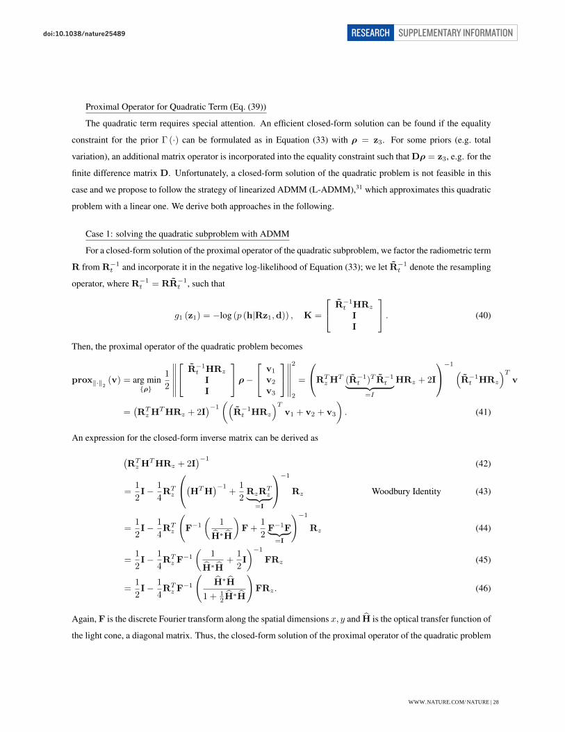
Proximal Operator for Quadratic Term (Eq. (39))

The quadratic term requires special attention. An efficient closed-form solution can be found if the equality

constraint for the prior � (·) can be formulated as in Equation (33) with ⇢ = z3. For some priors (e.g. total

variation), an additional matrix operator is incorporated into the equality constraint such that D⇢ = z3, e.g. for the

finite difference matrix D. Unfortunately, a closed-form solution of the quadratic problem is not feasible in this

case and we propose to follow the strategy of linearized ADMM (L-ADMM),31 which approximates this quadratic

problem with a linear one. We derive both approaches in the following.

Case 1: solving the quadratic subproblem with ADMM

For a closed-form solution of the proximal operator of the quadratic subproblem, we factor the radiometric term

R from R�1t

and incorporate it in the negative log-likelihood of Equation (33); we let R̃�1t

denote the resampling

operator, where R�1t

= RR̃�1t

, such that

g1 (z1) = �log (p (h|Rz1,d)) , K =

2

4R̃�1

t

HRz

II

3

5 . (40)

Then, the proximal operator of the quadratic problem becomes

proxk·k2(v) = arg min

{⇢}

1

2

��

2

4R̃�1

t

HRz

II

3

5⇢�2

4v1

v2

v3

3

5

��

2

2

=

0

@RT

z

HT (R̃�1t

)T R̃�1t| {z }

=I

HRz

+ 2I

1

A�1⇣R̃�1

t

HRz

⌘T

v

=�RT

z

HTHRz

+ 2I��1

✓⇣R̃�1

t

HRz

⌘T

v1 + v2 + v3

◆. (41)

An expression for the closed-form inverse matrix can be derived as

�RT

z

HTHRz

+ 2I��1

(42)

=1

2I� 1

4RT

z

0

@�HTH��1

+1

2R

z

RT

z| {z }=I

1

A�1

Rz

Woodbury Identity (43)

=1

2I� 1

4RT

z

F�1

✓1

bH⇤ bH

◆F+

1

2F�1F| {z }

=I

!�1

Rz

(44)

=1

2I� 1

4RT

z

F�1

✓1

bH⇤ bH+

1

2I

◆�1

FRz

(45)

=1

2I� 1

4RT

z

F�1

bH⇤ bH

1 + 12bH⇤ bH

!FR

z

. (46)

Again, F is the discrete Fourier transform along the spatial dimensions x, y and bH is the optical transfer function of

the light cone, a diagonal matrix. Thus, the closed-form solution of the proximal operator of the quadratic problem



is

proxk·k2(v) =

1

2I� 1

4RT

z

F�1bH⇤ bH

1 + 12bH⇤ bH

!FR

z

!✓⇣R̃�1

t

HRz

⌘T

v1 + v2 + v3

◆. (47)

This proximal operator can be efficiently evaluated for large-scale problems without explicitly forming any of the

matrices.

Case 2: approximating the quadratic subproblem with L-ADMM

If the choice of prior alters the equality constraints given by Equation (33), a closed-form solution of the

proximal operator of the quadratic subproblem may not exist. In this case, Equation (39) could be solved iteratively,

for example using the conjugate gradient (CG) method. However, this is computationally expensive because we

have to solve an iterative method (CG) embedded within another iterative method (ADMM). Instead, we propose to

use linearized ADMM (L-ADMM),31 where the quadratic subproblem is approximated with a linear one, resulting

in the following update in Equation (39):

⇢ proxk·k2(v) ⇡ ⇢� ⇢

µKT (K⇢� v) . (48)

This approach can be interpreted as a single step of a gradient descent approach with a step length of ⇢/µ. Conse-

quently, one would expect the linearized ADMM approach to converge slower than solving the quadratic subprob-

lem with the closed-form solution outlined above. Nevertheless, for certain priors which are incompatible with

the closed-form solution, linearized ADMM may be a good alternative. A suggested choice for the step length is

⇢/µ = 1/ kKk22 with ⇢ = 1/ kKk2.

Proximal Operator for Poisson Term (Eq. 35)

The specific splitting approach of Equation (40) requires the proximal operator of the Poisson term to include

the radiometric term R. Recall, this proximal operator is defined as

proxP,⇢

(v) = arg min{z1}

O (z1) = arg min{z1}

�log (p (h|Rz1,d)) +⇢

2kz1 � vk22 . (49)

Due to the fact that R is diagonal, the noisy observations are independent of each other, so we do not need to

account for the joint probability of all measurements. We write the ith element of the objective function O as

Oi

(z1) = �log✓(r

i

z1i

+ di

)h

i e�(riz1i

+d

i

) 1

hi

!

◆+

⇢

2(z1

i

� vi

)2 (50)

= �log (ri

z1i

+ di

)hi

+ (ri

z1i

+ di

)� log✓

1

hi

!

◆+

⇢

2(z1

i

� vi

)2

and its gradient as

@Oi

@z1i

= �ri

hi

ri

z1i

+ di

+ ri

+ ⇢ (z1i

� vi

) ,@O

i

@z1j

= 0 8i 6= j. (51)



Equating this gradient to zero results in a classical root-finding problem of a quadratic, which can be solved

independently for each z1i

. The quadratic has two roots, but due to the nonnegativity constraints in our objective

function we are only interested in the positive one. Thus, we can define the proximal operator as

proxP,⇢

(v) = �r2 + ⇢d� ⇢vr

2⇢r+

s✓r2 + ⇢d� ⇢vr

2⇢r

◆2

+rh+ ⇢dv � rd

⇢r. (52)

This operator is a closed-form solution that is independently applied to each pixel, i.e. all vector-vector multiplica-

tions, divisions, and exponentials in Equation (52) are performed element-wise. Note that we still need to choose a

parameter ⇢ for the ADMM updates. Heuristically, small values (e.g., 1e�5) work best for large signals with little

noise, but as the Poisson noise starts to dominate the image formation, ⇢ should be higher. For more details on

similar types of proximal operators, please refer to Dupe et al.32

Proximal Operator for Indicator Function (Eq. (36))

The proximal operator for the indicator function representing the constraints is straightforward

proxI,⇢ (v) = arg min{z2}

IR+ (z2) +⇢

2kv � z2k22 = arg min

{z22R+}kz2 � vk22 = ⇧R+ (v) , (53)

where ⇧R+ (·) is the element-wise projection operator onto the convex set R+

⇧R+ (vj

) =

⇢0 v

j

< 0vj

vj

� 0(54)

Proximal Operator for the Prior � (Eq. (37))

The objective function of Equation (37) is

prox�,⇢ (v) = arg min{z3}

� (z3) +⇢

2kv � z3k22 . (55)

A variety of priors, many with closed-form solutions, have been proposed.31 For example, total variation (TV) is

one of the most widely used priors in image reconstruction and has recently been proposed for denoising range data

captured with SPADs.24 For this choice of prior, solving Equation (55) amounts to a soft-thresholding operator31

where we impose the constraint z3 = D⇢, with D implementing a finite difference operator. However, the addition

of the matrix operator in the constraint complicates the closed-form solution of the quadratic ADMM subproblem

described in Case 1. Thus for the TV prior, or other priors which bring in additional terms to the constraints, the

L-ADMM approach can be used.

Other choices of priors include sparsity priors on the volume or self-similarity-type priors, such as non-local

means or BM3D. Many of these priors were recently studied in the context of denoising and deconvolution of

transient images;27 all of these priors or weighted combinations of them are equally applicable for NLOS imaging.



References

30 Arfken, G. Mathematical Methods for Physicists (Academic Press, 1985), third edn.

31 Boyd, S., Parikh, N., Chu, E., Peleato, B. & Eckstein, J. Distributed optimization and statistical learning via the

alternating direction method of multipliers. Foundations and Trends in Machine Learning 3, 1–122 (2011).

32 Dupe, F.-X., Fadili, M. & Starck, J.-L. Inverse problems with Poisson noise: primal and primal-dual splitting.

Int. Conference on Image Processing 1901–1904 (2011).



SU PPLEMENTARY INFORMATION - media. · PDF fileeral non-line-of-sight imaging approaches. The...

Documents

Transcript of SU PPLEMENTARY INFORMATION - media. · PDF fileeral non-line-of-sight imaging approaches. The...