Studying Recommendation Algorithms

by Graph Analysis

Batul J. MirzaDepartment of Computer Science

Virginia TechBlacksburg, VA 24061

bmirza@csgrad.cs.vt.edu

Benjamin J. KellerDepartment of Computer Science

Eastern Michigan UniversityYpsilanti, MI 48197

Ben.Keller@emich.edu

Naren RamakrishnanDepartment of Computer Science

Virginia TechBlacksburg, VA 24061naren@cs.vt.edu

Abstract

We present a novel framework for studying recommendation algorithms in terms of the‘jumps’ that they make to connect people to artifacts. This approach emphasizes reach-ability via an algorithm within the implicit graph structure underlying a recommenderdataset and allows us to consider questions relating algorithmic parameters to propertiesof the datasets. For instance, given a particular algorithm ‘jump,’ what is the averagepath length from a person to an artifact? Or, what choices of minimum ratings andjumps maintain a connected graph? We illustrate the approach with a common jumpcalled the ‘hammock’ using movie recommender datasets.

Keywords: Recommender Systems, Collaborative Filtering, Information System Eval-uation, Random Graphs.

1

1 Introduction

Recommender systems [41] constitute one of the fastest growing segments of the Interneteconomy today. They help reduce information overload and provide customized informationaccess for targeted domains. Building and deploying recommender systems has maturedinto a fertile business activity, with benefits in retaining customers and enhancing revenues.Elements of the recommender landscape include customized search engines, handcraftedcontent indices, personalized shopping agents on e-commerce sites, and news-on-demandservices. The scope of such personalization thus extends to many different forms of informa-tion content and delivery, not just web pages. The underlying algorithms and techniques,in turn, range from simple keyword matching of consumer profiles, collaborative filtering, tomore sophisticated forms of data mining, such as clustering web server logs.

Recommendation is often viewed as a system involving two modes (typically people andartifacts, such as movies and books) and has been studied in domains that focus on har-nessing online information resources, information aggregation, social schemes for decisionmaking, and user interfaces. A recurring theme among many of these applications is thatrecommendation is implicitly cast as a task of learning mappings (from people to recom-mended artifacts, for example) or of filling in entries to missing cells in a matrix (of consumerpreferences, for example). Consequently, recommendation algorithms are evaluated by theaccuracies of their predicted ratings. We approach recommendation from a different butcomplementary perspective of considering the connections that are made.

1.1 Motivating Scenarios

We describe three scenarios involving recommender system design to motivate the ideaspresented in this paper.

• Scenario 1: A small town bookstore is designing a recommender system to providetargeted personalization for its customers. Transactional data, from purchases cata-loged over three years, is available. The store is not interested in providing specificrecommendations of books, but is keen on using its system as a means of introducingcustomers to one another and encouraging them to form reading groups. It wouldlike to bring sufficiently concerted groups of people together, based on commonality ofinterests. Too many people in a group would imply a diffusion of interests; modelingreading habits too narrowly might imply that some people cannot be matched withanybody. How can the store relate commonality of interests to the sizes of clusters ofpeople that are brought together?

• Scenario 2: An e-commerce site, specializing in books, CDs, and movie videos, isinstalling a recommendation service. The designers are acutely aware that peoplebuy and rate their different categories of products in qualitatively different ways. Forexample, movie ratings follow a hits-buffs distribution: some people (the buffs) see/ratealmost all movies, and some movies (the hits) are seen/rated by almost all people.Music CD ratings are known to be more clustered, with hits-buffs distributions visibleonly within specific genres (like ‘western classical’). Connections between differentgenres are often weak, compared to connections within a genre. How can the designersreason about and visualize the structure of these diverse recommendation spaces, toallow them to custom-build their recommendation algorithms?

2

• Scenario 3: An online financial firm is investing in a recommendation service and isrequiring each of its members to rate at least κ products of their own choice to ensurethat there are enough overlaps among ratings. The company’s research indicates thatpeople’s ratings typically follow power-law distributions. Furthermore, the company’smarketers have decided that recommendations of ratings can be explainably transferredfrom one person to another if they have at least 6 ratings in common. Given thesestatistics and design constraints, what value of κ should be set by the company to ensurethat every person (and every product) is reachable by its recommendation service?

The common theme among these applications is that they emphasize many important aspectsof a recommender system other than predictive accuracy: its role as an indirect way ofbringing people together, its signature pattern of making connections, and the explainabilityof its recommendations. To address the questions raised by considering these aspects ofrecommendation, we propose a framework based on a mathematical model of the socialnetwork implicit in recommendation. This framework allows a more direct approach toreasoning about recommendation algorithms and their relationship to the recommendationpatterns of users. We effectively ignore the issue of predictive accuracy, and so the frameworkis a complement to approaches based on field studies.

The defined framework depends only on connections between people and artifacts, andso merely requires that we can capture the effect of a recommendation algorithm in suchterms. This does not mean that the framework only applies to collaborative filtering whereuser-artifact relationships are explicitly collected. Other approaches that implicitly connecta user to an artifact can also be studied in this framework (e.g., by web page visits, using co-occurrence patterns). Algorithms that use direct measures of the similarity of the attributesof users (e.g., age) can also be modeled, although we do not describe how in this paper.

Our framework allows a novel strategy for characterizing a recommender algorithm interms of the connections that it makes. We explore the foundations of this strategy for ageneralization of the connections made by most common (collaborative filtering) algorithms.In particular, we look at characteristics of the social network graph induced by this algorithm,relating to whether recommendations can be made (connectivity of the social network) andhow much effort is required (path lengths in the social network).

1.2 Reader’s Guide

Section 2 surveys current research and motivates the need for a new approach to analyzingalgorithms for recommender systems. Section 3 introduces the jumping connections frame-work and develops a mathematical model based on random graph theory. Section 4 providesexperimental results for one particular way of jumping on two application datasets. Issuesrelated to interpretation of results from our model are also presented here. Finally, Section 5identifies some opportunities for future research.

2 Characterizing Recommendation Algorithms

Most current research efforts cast recommendation as a specialized task of information re-trieval/filtering or as a task of function approximation/learning mappings [2, 7, 8, 19, 20,23, 24, 27, 31, 39, 46, 47, 48, 50, 51, 53]. Even approaches that focus on clustering view

3

clustering primarily as a pre-processing step for functional modeling [30], or as a technique toensure scalability [37, 47] or to overcome sparsity of ratings [54]. This emphasis on functionalmodeling and retrieval has influenced evaluation criteria for recommender systems.

Traditional information retrieval evaluation metrics such as precision and recall havebeen applied toward recommender systems involving content-based design. Ideas such ascross-validation on an unseen test set have been used to evaluate mappings from people toartifacts, especially in collaborative filtering recommender systems. Such approaches missmany desirable aspects of the recommendation process, namely:

• Recommendation is an indirect way of bringing people together. As we willdiscuss recommendation algorithms, especially collaborative filtering, exploit connec-tions between users and artifacts. Social network theory [55] can be used to model sucha recommendation system of people versus artifacts as an affiliation network and dis-tinguishes between a primary mode (e.g., people) and a secondary mode (e.g., movies),where a mode refers to a distinct set of entities that have similar attributes [55]. Thepurpose of the secondary mode is viewed as serving to bring entities of the primarymode together (i.e., it isn’t treated as a first-class mode).

• Recommendation, as a process, should emphasize modeling connectionsfrom people to artifacts, besides predicting ratings for artifacts. In many sit-uations, users would like to request recommendations purely based on local and globalconstraints on the nature of the specific connections explored. Functional modelingtechniques are inadequate because they embed the task of learning a mapping frompeople to predicted values of artifacts in a general-purpose learning system such asneural networks or Bayesian classification [10]. A notable exception is the work byHofmann and Puzicha [25] which allows the incorporation of constraints in the formof aspect models involving a latent variable.

• Recommendations should be explainable and believable. The explanationsshould be made in terms and constructs that are natural to the user/application do-main. It is nearly impossible to convince the user of the quality of a recommendationobtained by black-box techniques such as neural networks. Furthermore, it is wellrecognized that “users are more satisfied with a system that produces [bad recommen-dations] for reasons that seem to make sense to them, than they are with a systemthat produces [bad recommendations] for seemingly stupid reasons” [44].

• Recommendations are not delivered in isolation, but in the context of animplicit/explicit social network. In a recommender system, the rating patterns ofpeople on artifacts induce an implicit social network and influence the connectivitiesin this network. Little study has been done to understand how such rating patternsinfluence recommendations and how they can be advantageously exploited.

Our approach in this paper is to study recommendation algorithms using ideas fromgraph analysis. In the next section, we will show how our viewpoint addresses each of theabove aspects, by providing novel metrics. The basic idea is to begin with data that canbe modeled as a network and attempt to infer useful knowledge from the vertices and edgesof the graph. Vertices represent entities in the domain (e.g., people, movies), and edgesrepresent the relationships between entities (e.g., the act of a person viewing a particularmovie).

4

2.1 Related Research

The idea of graph analysis as a basis to study information networks has a long tradition; oneof the earliest pertinent studies is Schwartz and Wood [49]. The authors describe the useof graph-theoretic notions such as cliques, connected components, cores, clustering, averagepath distances, and the inducement of secondary graphs. The focus of the study was tomodel shared interests among a web of people, using email messages as connections. Suchlink analysis has been used to extract information in many areas such as in web searchengines [28], in exploration of associations among criminals [42], and in the field of medicine[52]. With the emergence of the web as a large scale graph, interest in information networkshas recently exploded [1, 11, 12, 14, 17, 26, 28, 29, 32, 38, 40, 56].

Most graph-based algorithms for information networks can be studied in terms of (i) thegraph modeling (e.g., what are the modes?, how do they relate to the information domain?),and (ii) the structures/operations that are mined/conducted on the graph. One of themost celebrated examples of graph analysis arises in search engines that exploit both linkinformation and textual content. The Google search engine uses the web’s link structure inaddition to the anchor text, as a factor in ranking pages based on the pages that (hyper)linkto the given page [11]. Google essentially models a one-mode directed graph (of web pages)and uses measures involving principal components to ascertain ‘page ranks.’ Jon Kleinberg’sHITS (Hyperlink-Induced Topic Search) algorithm goes a step further by viewing the one-mode web graph as actually comprising two modes (called hubs and authorities) [28]. Ahub is a node primarily with edges to authorities, and so a good hub has links to manyauthorities. A good authority is a page that is linked to by many hubs. Starting with aspecific search query, HITS performs a text-based search to seed an initial set of results.An iterative relaxation algorithm then assigns hub and authority weights using a matrixpower iteration. Empirical results show that remarkably authoritative results are obtainedfor search queries. The CLEVER search engine is built primarily on top of the basic HITSalgorithm [14].

The use of link analysis in recommender systems was highlighted by the “referral chain-ing” technique of the ReferralWeb project [26]. The idea is to use the co-occurrence of namesin any of the documents available on the web to detect the existence of direct relationshipsbetween people and discover a social network. The underlying assumption is that peoplewith similar interests swarm in the same circles to discover collaborators [38].

The exploration of link analysis in social structures has led to several new avenues ofresearch, most notably small-world networks. Small-world networks are highly clustered butrelatively sparse networks with small average length. An example is the folklore notion ofsix degrees of separation separating any two people in our universe: the phenomenon wherea person can discover a link to any other random person through a chain of at most sixacquaintances. A small-world network is sufficiently clustered so that most second neighborsof a node X are also neighbors of X (a typical ratio would be 80%). On the other hand, theaverage distance between any two nodes in the graph is comparable to the low characteristicpath length of a random graph. Until recently, a mathematical characterization of suchsmall-world networks has proven elusive. Watts and Strogatz [56] provide the first suchcharacterization of small-world networks in the form of a graph generation model.

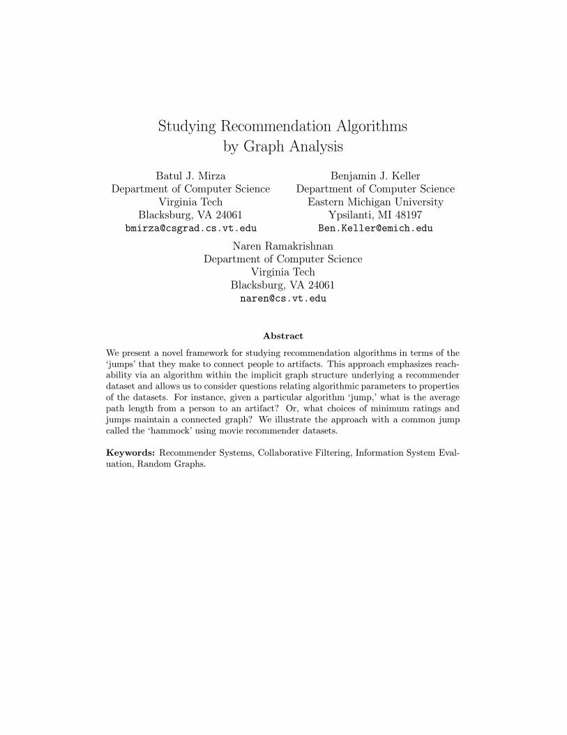
In this model, Watts and Strogatz use a regular wreath network with n nodes, and kedges per node (to its nearest neighbors) as a starting point for the design. A small fraction

5

p = 1p= 0

Increasing randomness

Random NetworkSmall-World NetworkRegular Network

Figure 1: Generation of a small-world network by random rewiring from a regular wreathnetwork. Figure adapted from [56].

10-4

10-3

10-2

10-1

100

0

0.1

0.2

0.3

0.4

0.5

0.6

0.7

0.8

0.9

1

Probability p

Average LengthAverage Clustering Coefficient

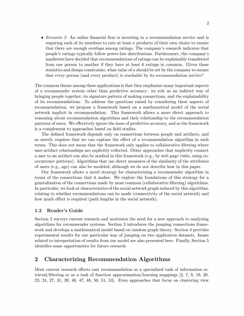
Figure 2: Average path length and clustering coefficient versus the rewiring probability p(from [56]). All measurements are scaled w.r.t. the values at p = 0.

6

of the edges are then randomly rewired to arbitrary points on the network. A full rewiring(probability p = 1) leads to a completely random graph, while p = 0 corresponds to the(original) wreath (Fig. 1). The starting point in the figure is a regular wreath topologyof 12 nodes with every node connected to its four nearest neighbors. This structure has ahigh characteristic path length and high clustering coefficient. The average length is themean of the shortest path lengths over all pairs of nodes. The clustering coefficient is de-termined by first computing the local neighborhood of every node. The number of edges inthis neighborhood as a fraction of the total possible number of edges denotes the extent ofthe neighborhood being a clique. This factor is averaged over all nodes to determine theclustering coefficient. The other extreme in Fig. 1 is a random network with a low char-acteristic path length and almost no clustering. The small-world network, an interpolationbetween the two, has the low characteristic path length (of a random network), and retainsthe high clustering coefficient (of the wreath). Measuring properties such as average lengthand clustering coefficient in the region 0 ≤ p ≤ 1 produces surprising results (see Fig. 2).

As shown in Fig. 2, only a very small fraction of edges need to be rewired to bring thelength down to random graph limits, and yet the clustering coefficient is high. On closerinspection, it is easy to see why this should be true. Even for small values of p (e.g., 0.1), theresult of introducing edges between distantly separated nodes reduces not only the distancebetween these nodes but also the distances between the neighbors of those nodes, and soon (these reduced paths between distant nodes are called shortcuts). The introduction ofthese edges further leads to a rapid decrease in the average length of the network, but theclustering coefficient remains almost unchanged. Thus, small-world networks fall in betweenregular and random networks, having the small average lengths of random networks but highclustering coefficients akin to regular networks.

While the Watts-Strogatz model describes how small-world networks can be formed, itdoes not explain how people are adept at actually finding short paths through such networksin a decentralized fashion. Kleinberg addresses precisely this issue and proves that this isnot possible in the family of one-dimensional Watts-Strogatz networks [29]. Embedding thenotion of random rewiring in a two-dimensional lattice leads to one unique model for whichsuch decentralization is effective.

The small-world network concept has implications for a variety of domains. Watts andStrogatz simulate the spread of an infectious disease in a small-world network [56]. Adamicshows that the world wide web is a small-world network and suggests that search enginescapable of exploiting this fact can be more effective in hyperlink modeling, crawling, andfinding authoritative sources [1].

Besides the Watts-Strogatz model, a variety of models from graph theory are availableand can be used to analyze information networks. Kumar et al. [32] highlight the useof traditional random graph models to confirm the existence of properties such as coresand connected components in the web. In particular, they characterize the distributions ofweb page degrees and show that they are well approximated by power laws. Finally, theyperform a study similar to Schwartz and Wood [49] to find cybercommunities on the web.Flake et al. [17] provide a max-flow, min-cut algorithm to identify cybercommunities. Theyalso provide a focused crawling strategy to approximate such communities. Broder et al. [12]perform a more detailed mapping of the web and demonstrate that it has a bow-tie structure,which consists of a strongly connected component, as well as nodes that link into but arenot linked from the strongly connected component, and nodes that are linked from but do

7

not link to the strongly connected component. Pirolli et al. [40] use ideas from spreadingactivation theory to subsume link analysis, content-based modeling, and usage patterns.

A final thread of research, while not centered on information networks, emphasizes themodeling of problems and applications in ways that make them amenable to graph-basedanalyses. A good example in this category is the approach of Gibson et al. [18] for miningcategorical datasets.

While many of these ideas, especially link analysis, have found their way into recom-mender systems, they have been primarily viewed as mechanisms to mine or model struc-tures. In this paper, we show how ideas from graph analysis can actually serve to characterizerecommender algorithms.

3 Graph Analysis

In the previous section, we identified four pertinent aspects of recommendation:

• bringing people together by connections; in

• an underlying graph-theoretic structure;

• explainability; and

• modeling of social networks.

To address these four aspects, we develop a novel way to study algorithms for recommendersystems. Algorithms are distinguished, not by the predicted ratings of services/artifacts theyproduce, but by the combinations of people and artifacts that they bring together. Twoalgorithms are considered equivalent if they bring together identical sets of nodes regardlessof whether they work in qualitatively different ways. Our emphasis is on the role of arecommender system as a mechanism for bridging entities in a social network. We refer tothis approach of studying recommendation as jumping connections.

Notice that the framework does not emphasize how the recommendation is actually made,or the information that an algorithm uses to make connections (e.g., does it rely on others’ratings, on content-based features, or both?). In addition, we make no claims about therecommendations being better or that they will be better received. Our metrics, hence,will not lead a designer to directly conclude that an algorithm A is more accurate thanan algorithm B; such conclusions can only be made through a field evaluation (involvingfeedback and reactions from users) or via survey/interview procedures. By restricting itsscope to exclude the actual aspect of making ratings and predictions, the jumping connectionsframework provides a systematic and rigorous way to study recommender systems.

Of course, the choice of how to jump connections will be driven by the (often conflicting)desire to reach almost every node in the graph (i.e., recommend every product for somebody,or recommend some product for everybody) and the strength of the jumps enjoyed when twonodes are brought together. The conflict between these goals can be explicitly expressed inour framework.

It should be emphasized that our model doesn’t imply that algorithms only exploit localstructure of the recommendation dataset. Any mechanism — local or global — could be

8

used to jump connections. In fact, it is not even necessary that algorithms employ graph-theoretic notions to make connections. Our framework only requires a boolean test to see iftwo nodes are brought together.

Notice also that when an algorithm brings together person X and artifact Y , it couldimply either a positive recommendation or a negative one. Such differences are, again, notcaptured by our framework unless the mechanism for making connections restricts its jumps,for instance, to only those artifacts for which ratings satisfy some threshold. In other words,thresholds for making recommendations could be abstracted into the mechanism for jumping.

Jumping connections satisfies all the aspects outlined in the previous section. It involves asocial-network model, and thus, emphasizes connections rather than prediction. The natureof connections jumped also aids in explaining the recommendations. The graph-theoreticnature of jumping connections allows the use of mathematical models (such as randomgraphs) to analyze the properties of the social networks in which recommender algorithmsoperate.

3.1 The Jumping Connections Construction

We now develop the framework of jumping connections. We use concepts from a movierecommender system to provide the intuition; this does not restrict the range of applicabilityof jumping connections and is introduced here only for ease of presentation.

A recommender dataset R consists of the ratings by a group of people of movies in acollection. The ratings could in fact be viewings, preferences, or other constraints on movierecommendations. Such a dataset can be represented as a bipartite graph G = (P ∪M,E)where P is the set of people, M is the set of movies, and the edges in E represent the ratingsof movies. We denote the number of people by NP = |P |, and the number of movies asNM = |M |.

We can view the set M as a secondary mode that helps make connections — or jumps —between members of P . A jump is a function J : R 7→ S, S ⊆ P × P that takes as input arecommender dataset R and returns a set of (unordered) pairs of elements of P . Intuitively,this means that the two nodes described in a given pair can be reached from one anotherby a single jump. Notice that this definition does not prescribe how the mapping shouldbe performed, or whether it should use all the information present in R. We also make theassumption that jumps can be composed in the following sense: if node B can be reachedfrom A in one jump, and C can be reached from B in one jump, then C is reachable from Ain two jumps. The simplest jump is the skip, which connects two members in P if they haveat least one movie in common.

A jump induces a graph called a social network graph. The social network graph ofa recommender dataset R induced by a given jump J is a unipartite undirected graphGs = (P,Es), where the edges are given by Es = J (R). Notice that the induced graphcould be disconnected based on the strictness of the jump function. Figure 3 (b) shows thesocial network graph induced from the example in Figure 3 (a) using a skip jump.

We view a recommender system as exploiting the social connections (the jumps) thatbring together a person with other people who have rated an artifact of (potential) interest.To model this, we view the unipartite social network of people as a directed graph andreattach movies (seen by each person) such that every movie is a sink (reinforcing its role asa secondary mode). The shortest paths from a person to a movie in this graph can then be

9

p2

p3

p4p5

p1

J

m1

m2

m4

p1

p2

p3

p4

p5

m3

(c)

(b)

(a)

m1

m2

m3

m4

p2

p3

p1

p5

p4

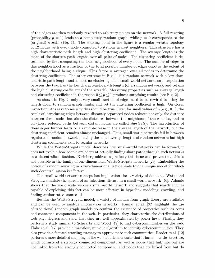
Figure 3: Illustration of the skip jump. (a) bipartite graph of people and movies. (b) Socialnetwork graph, and (c) recommender graph.

used to provide the basis for recommendations. We refer to a graph induced in this fashionas a recommender graph (Figure 3 (c)). Since the outdegree of every movie node is fixed atzero, paths through the graph are from people to movies (through more people, if necessary).

The recommender graph of a recommender dataset R induced by a given jump functionJ is a directed graph Gr = (P ∪M,Esd ∪Emd), where Esd is an ordered set of pairs, listingevery pair from J (R) in both directions, and Emd is an ordered set of pairs, listing everypair from E in the direction pointing to the movie mode.

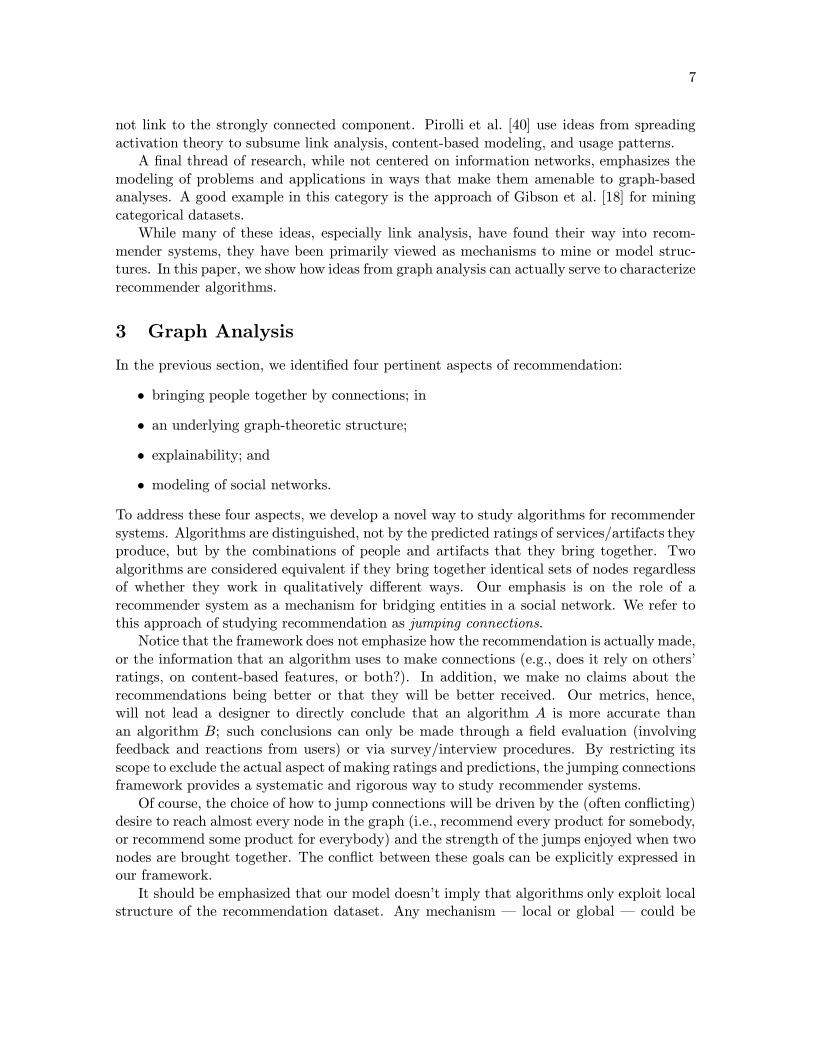
Assuming that the jump construction does not cause Gr to be disconnected, the portionof Gr containing only people is its strongest component: every person is connected to everyother person. The movies constitute vertices which can be reached from the strongest com-ponent, but from which it is not possible to reach the strongest component (or any othernode, for that matter). Thus, Gr can be viewed as a ‘half bow-tie,’ (Figure 4) as contrastedto the full bow-tie nature of the web, observed by Broder et al. [12]. The circular portionin the figure depicts the strongly connected component derived from Gs. Links out of thisportion of the graph are from people nodes and go to sinks, which are movies.

3.2 Basic Approach

The skip jump is admittedly a simplistic way to model a recommendation algorithm and isintroduced here only for illustration. A realistic recommendation algorithm would be morecareful in bringing people nodes together; it might consider aspects such as commonality ofrated artifacts, agreement among ratings, correlations, and other metrics of statistical simi-larity. There are thus many ways of inducing the social network graph and the recommendergraph.

Our basic approach is to think of the operation of a given recommendation algorithmas performing a jump and study this jump algorithmically using tools from random graphtheory. Our specific contributions in this paper are the emphasis on graph analysis as a way to

10

p4

p2p1

p3

p5

m1

m2

m4

m3

Figure 4: The jumping connections construction produces a half bow-tie graph Gr.

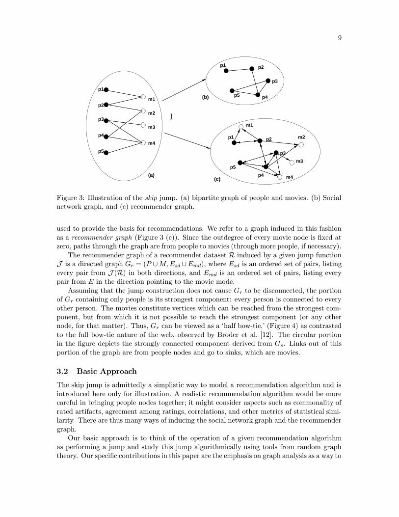
Figure 5: A path of hammock jumps, with a hammock width w = 4.

11

study recommendation algorithms and the use of random graph models to predict propertiesof interest about the social network and recommender graphs. The mathematical machinerybrought to bear upon this problem is the work of Newman, Strogatz, and Watts [36]; theuse of these formulas for studying recommendation algorithms is novel here.

For want of space, we are unable to study all or even a considerable number of jumpsfrom the recommender systems literature. Instead, we focus on one jump called the hammockjump and describe the full extent of the analyses that can be conducted within our proposedframework. A more comprehensive list of jumps defined by different algorithms is exploredby Mirza [35].

3.3 Hammocks

A hammock jump brings two people together in Gs if they have at least w movies in commonin R. Formally, a pair (p1, p2) is in J (R) whenever there is a set M(p1,p2) of w movies suchthat there is an edge from p1 and p2 to each element of M(p1,p2). The number w of commonartifacts is called the hammock width. Figure 5 illustrates a sequence (or hammock path) ofhammocks.

There is some consensus in the community that hammocks are fundamental in rec-ommender algorithms since they represent commonality of ratings. It is our hypothesisthat hammocks are fundamental to all recommender system jumps. Early recommendationprojects such as GroupLens [31], LikeMinds [33], and Firefly [50] can be viewed as employing(simple versions of) hammock jumps involving at most one intermediate person.

The horting algorithm of Aggarwal et al. [2] extends this idea to a sequence of hammockjumps. Two relations — horting and predictability — are used as the basis for a jump. Aperson p1 horts person p2 if the ratings they have in common are a sufficiently large subset ofthe ratings of p1. A person predicts another if they have a reverse horting relationship, andif there is a linear transformation between their ratings. The algorithm first finds shortestpaths of hammocks that relate to predictability and then propagates ratings using the lineartransformations. The implementation described by Aggarwal et al. [2] uses a bound on thelength of the path.

There are a number of interesting algorithmic questions that can be studied. First,since considering more common ratings can be beneficial (see [23] for approaches) having awider hammock could be better (this is not exactly true, when correlations between ratingsare considered [23]). Second, many recommender systems require a minimum number κ ofratings before the user may use the system, to prevent free-riding on recommendations [5].What is a good value for κ? And, third what is the hammock diameter or how far would wehave to traverse to reach everyone in the social network graph? We begin looking at thesequestions in the next section.

3.4 Random Graph Models

Our goal is to be able to answer questions about hammock width, minimum ratings, andpath length in a typical graph. The approach we take is to use a model of random graphsadapted from the work of Newman, Strogatz, and Watts [36]. This model, while havinglimitations, is the best-fit of existing models, and as we shall see, provides imprecise butdescriptive results.

12

A recommender dataset R can be characterized by the number of ratings that each per-son makes, and the number of ratings that each artifact receives. These values correspondto the degree distributions in the bipartite rating graph for R. These counts are relativelyeasy to obtain from a dataset and so could be used in the analysis of recommender algo-rithms. Therefore, we would like to be able to characterize a random bipartite graph usingparticular degree distributions. This requirement means that the more common randomgraph models (e.g., [15]) are not appropriate, since they assume that edges occur with equalprobability. On the other hand, a model recently proposed by Aiello, Chung, and Lu [3] isbased on a power-law distribution, similar to characteristics observed of actual recommen-dation datasets (see next section). But again this model is not directly parameterized bythe degree distribution. The Newman-Strogatz-Watts model is the only (known) model thatcharacterizes a family of graphs in terms of degree distributions.

From the original bipartite graph G = (P ∪M,E) for R we develop two models, one forthe social network graph Gs and one for the recommender graph Gr.

3.5 Modeling the Social Network Graph

Recall that the social network graph Gs = (P,Es) is undirected and Es is induced by a jumpfunction J on R. The Newman-Strogatz-Watts model works by characterizing the degreedistribution of the vertices, and then using that to compute the probability of arriving at anode. Together they describe a random process of following a path through a graph, andallow computations of the length of paths. Here we only discuss the equations that are used,and not the details of their derivation. The application of these equations to these graphs isoutlined by Mirza [35] and is based on the derivation by Newman et al. [36].

We describe the social network graph Gs by the probability that a vertex has a particulardegree. This is expressed as a generating function G0(x)

G0(x) =∞∑

k=0

pkxk,

where pk is the probability that a randomly chosen vertex in Gs has degree k. This functionmust satisfy the property that

G0(1) =∞∑

k=0

pk = 1.

To obtain an expression that describes the typical length of a path, we can consider howmany steps we need to go from a node to be able to get to every other node in the graph. Todo this we can use the number of neighbors k steps away. For a randomly chosen vertex inthis graph, G0(x) gives us the distribution of the immediate neighbors of that vertex. So, wecan compute the average number of vertices z1 one edge away from a vertex as the averagedegree z:

z1 = z =∑

k

kpk = G′0(1)

The number of neighbors two steps away is given by

z2 =∑

k

kpk1

z

∑

k

k(k − 1)pk

13

It turns out (see [36] for details) that the number of neighbors m steps away is given in termsof these two quantities:

zm =

(z2

z1

)m−1

z1

The path length lpp we are interested in is the one that is big enough to reach all of the NP

elements of P , and so lpp should satisfy the equation

1 +

lpp∑

m=1

zm = NP

where the constant 1 counts the initial vertex. Using this equation, it can be shown that thetypical length from one node to another in Gs is

lpp =log[(NP − 1)(z2 − z1) + z2

1 ]− log[z21]

log[z2/z1](1)

We use this formula as our primary means of computing the distances between pairs of peoplein Gs in the empirical evaluation in the next section. Since we use actual datasets, we cancompute pk as the fraction of vertices in the graph having degree k.

3.6 Modeling the Recommender Graph

The recommender graph Gr = (P ∪M,Esd∪Emd) is directed, and hence Newman, Strogatz,and Watts [36] capture both indegrees and outdegrees in a generating function:

G(x, y) =j=∞,k=∞∑

j=0,k=0

pjkxjyk,

where pjk is the probability that a randomly chosen vertex has indegree j and outdegree k.From the jumping connections construction, we know that movie vertices have outdegree

0 (the converse is not true, vertices with outdegree 0 could be people nodes isolated as aresult of a severe jump constraint). Notice also that by using the joint distribution pij ,independence of the indegree and outdegree distributions is not implied. We show in thenext section that this feature is very useful. In addition, the average number of arcs entering(or leaving) a vertex is zero. And, so

∑

jk

(j − k)pjk =∑

jk

(k − j)pjk = 0.

We arrive at new expressions for z1 and z2 [35]:

z1 =∑

jk

kpjk .

z2 =∑

jk

jkpjk.

The average path length lr can be calculated as before:

lr =log[(NP + NM − 1)(z2 − z1) + z2

1 ]− log[z21]

log[z2/z1], (2)

14

where NP + NM is the size of the recommender graph Gr (assuming that the graph is onegiant component), with NM denoting the number of movies. The length lr includes pathsfrom people to movies, as well as paths from people to people. The average length of onlyreaching movies from people lpm can be expressed as:

lpm =(lr(NP (NP − 1) + NPNM)− lppNP (NP − 1))

NPNM(3)

3.7 Caveats with the Newman-Strogatz-Watts Equations

There are various problems with using the above formulas in a realistic setting [21]. First,unlike most results in random graph theory, the formulas do not include any guaranteesand/or confidence levels. Second, all the equations above are obtained over the ensembleof random graphs that have the given degree distribution, and hence assume that all suchgraphs are equally likely. The specificity of the jumping connections construction impliesthat the Gs and Gr graphs are poor candidates to serve as a typical random instance of agraph.

In addition, the equations utilizing NP and NM assume that all vertices are reachablefrom any starting vertex (i.e., the graph is one giant component). This will not be satisfiedfor very strict jumping constraints. In such cases, Newman, Strogatz, and Watts suggestthe substitution of these values with measurements taken from the largest component ofthe graph. Expressing the size of the components of the graph using generating functionsis also suggested [36]. However, the complexity of jumps such as the hammock can makeestimation of the cluster sizes extremely difficult, if not impossible (in the Newman-Strogatz-Watts model). We leave this issue to future research.

Finally, the Newman-Strogatz-Watts model is fundamentally more complicated than tra-ditional models of random graphs. It has a potentially infinite set of parameters (pk), doesn’taddress the possibility of multiple edges, loops and, by not fixing the size of the graph, as-sumes that the same degree distribution sequence applies for all graphs, of all sizes. Theseobservations hint that we cannot hope for more than a qualitative indication of the depen-dence of the average path length on the jump constraints. In the next section, we describehow well these formulas perform on two real-world datasets.

4 Experimental Results

We devote this section to an investigation of two actual datasets from the movies domain;namely the EachMovie dataset, collected by the Digital Equipment Corporation (DEC)Systems Research Center, and the MovieLens [43] dataset developed at the University ofMinnesota. Both these datasets were collected by asking people to log on to a website andrate movies. The time spent rating movies was repaid by providing predictions of ratingsfor other movies not yet seen, which the recommendation engines calculated based on thesubmitted ratings and some other statistical information.

The datasets contain some basic demographic information about the people (age, gender,etc) as well the movies (title, genre, release date, etc). Associated with each person and movieare unique ids. The rating information (on a predefined numeric scale) is provided as a setof 3−tuples: the person id, the movie id, and the rating given for that movie by that person.Some statistics for both the datasets are provided in Table 1. Notice that only a small

15

Table 1: Some statistics for the EachMovie and MovieLens datasets.

Dataset Number of people Number of movies Sparsity Connected?

MovieLens 943 1,682 93.70% Yes

EachMovie 61,265 1,623 97.63% Yes

MOVIES

PEO

PLE

Figure 6: Hits-buffs structure of the (reordered) MovieLens dataset.

number of actual ratings are available (as a fraction of all possible combinations), and yetthe bipartite graphs of people versus movies are connected, in both cases.

4.1 Preliminary Investigation

Both the EachMovie and MovieLens datasets exhibit a hits-buffs structure. Assume thatpeople are ordered according to a buff index b: A person with buff index 1 has seen themost number of movies, a person with buff index 2 has seen the second most number ofmovies, and so on. For example, in the EachMovie dataset, the person with buff index 1has seen 1,455 movies from the total of 1,623. These 1,455 movies have, in turn, been seenby 61,249 other people. Thus, within two steps, a total of 62,705 nodes in the graph can bevisited; with other choices of the intermediate buff node, the entire graph can be shown tobe connected in, at the most, two steps. The MovieLens dataset satisfies a similar property.

Furthermore, the relationship between the buff index b and the number of movies seenby the buff P (b) follows a power-law distribution, with an exponential cutoff:

P (b) ∝ b−αe− bτ

For the EachMovie dataset, α ≈ 1.3 and τ ≈ 10,000. Similar trends can be observed forthe hits and for the MovieLens dataset. Graphs with such power-law regimes can thus formsmall-worlds [4] as evidenced by the short length between any two people in both MovieLensand EachMovie. To better demonstrate the structure, we reorder the people and movie ids,so that the relative positioning of the ids denotes the extent of a person being a buff, or amovie being a hit. For example, person id 1 refers to the person with buff index 1 and movieid 1 refers to the movie with hit index 1. Figure 6 illustrates the hits-buffs structure of theMovieLens dataset.

16

0 5 10 15 20 25 300

50

100

150

200

250

Hammock width wN

umbe

r of

com

pone

nts

Figure 7: Effect of the hammock width on the number of components in the Gr graphinduced from the MovieLens dataset.

4.2 Experiments

The goal of our experiments is to investigate the effect of the hammock width w on the aver-age characteristic path lengths of the induced Gs social network graph and Gr recommendergraph for the above datasets. We use versions of the EachMovie and MovieLens datasetssanitized by removing the rating information. So, even though rating information can easilybe used by an appropriate jump function (an example is given in [2]), we explore a purelyconnection-oriented jump in this study. Then, for various values of the hammock width w,we form the social network and recommender graphs and calculate the degree distributions(for the largest connected component). This was used to obtain the lengths predicted byequations 1 and 2 from Section 3. We also compute the average path length for the largestconnected component of both the secondary graphs using parallel implementations of Djik-stra’s and Floyd’s algorithms. The experimental observations are compared with the formulapredictions.

4.2.1 MovieLens

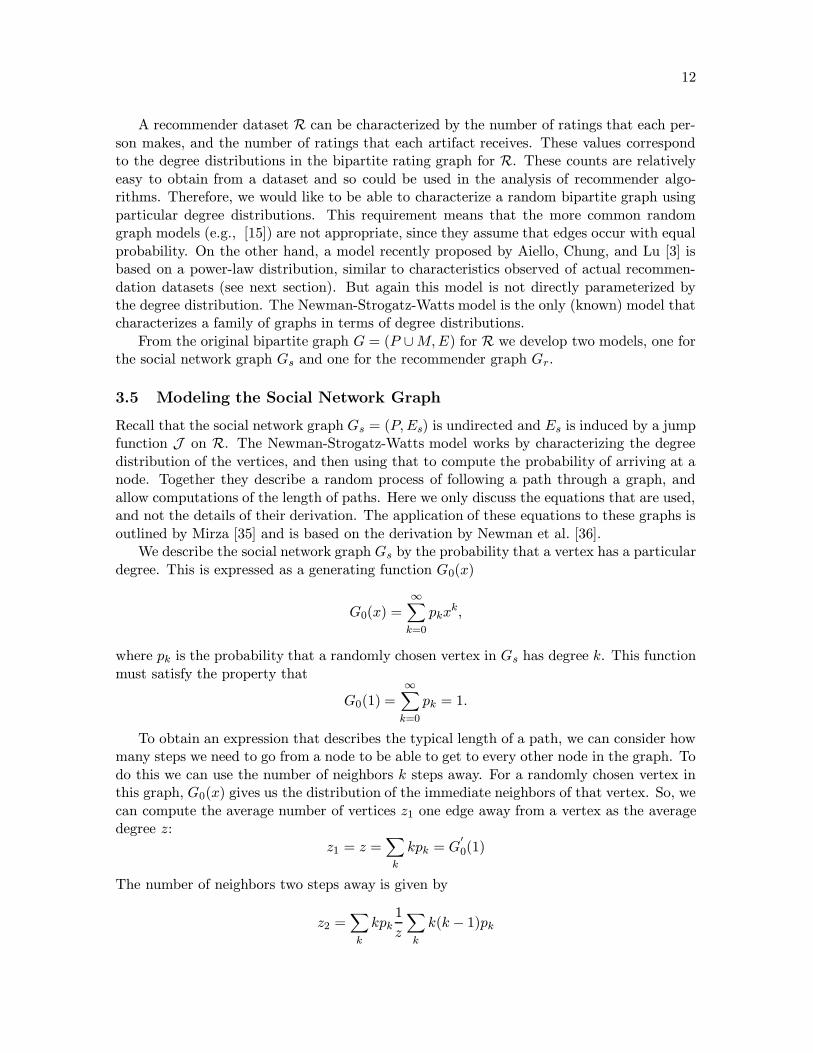
Fig. 7 describes the number of connected components in Gr as a result of imposing increas-ingly strict hammock jump constraints. Up to about w = 17, the graph remains in onepiece and rapidly disintegrates after this threshold. The value of this transition thresholdis not surprising, since the designers of MovieLens insisted that every participant rate atleast κ = 20 movies. As observed from our experiment results, after the threshold and upto w = 28, there is still only one giant component with isolated people nodes (Fig. 8, left).Specifically, the degree distributions of the MovieLens social network graphs for w > 17 showus that the people nodes that are not part of the giant component do not form any otherconnected components and are isolated. We say that a jump shatters a set of nodes if thevertices that are not part of the giant component do not have any edges. This aspect ofthe formation of a giant component is well known from random graph theory [9]. Since ourconstruction views the movies as a secondary mode, we can ensure that only the strictesthammock jumps shatter the NM movie nodes. Fig. 8 (right) demonstrates that the movienodes are not stranded as a result of hammock constraints up to hammock width w = 29.

The comparison of experimental observations with formula predictions for the lpp and lr

17

0 5 10 15 20 25 30700

750

800

850

900

950

Hammock width w

Num

ber

of p

eopl

e in

larg

est c

ompo

nent

0 5 10 15 20 25 301500

1520

1540

1560

1580

1600

1620

1640

1660

1680

1700

Hammock width w

Num

ber

of m

ovie

s in

larg

est c

ompo

nent

Figure 8: (left) Effect of the hammock width on the number of people in the largest com-ponents in the MovieLens Gr graph. (right) Effect of the hammock width on the number ofmovies in the largest components in the MovieLens Gr graph.

0 5 10 15 20 25 301

1.1

1.2

1.3

1.4

1.5

1.6

1.7

1.8

Hammock width w

Ave

rage

l pp le

ngth

Length from actual experimentsLength from formulas

0 5 10 15 20 25 301.2

1.3

1.4

1.5

1.6

1.7

1.8

1.9

2

Hammock width w

Ave

rage

l r leng

th Length from actual experimentsLength from formulas

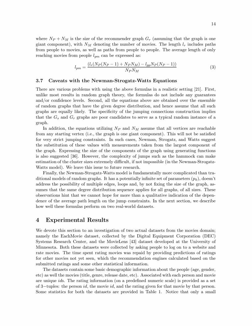
Figure 9: (left) Comparison of the lpp measure (MovieLens) from actual computations andfrom the formulas. (right) Comparison of the lr measure (MovieLens) from actual compu-tations and from the formulas.

lengths are shown in Fig. 9. The graphs for lpp share certain important characteristics. Theincrease in length up to the threshold point is explained by the fact that edges are removedfrom the giant component, meaning paths of greater length have to be traversed to reachother nodes. After the threshold, the relative stability of the length indicates that the onlyedges lost are those that are associated with the stranded people nodes. We attribute thefact that the lengths are between 1 and 2 to the hits-buffs structure, which allows short pathsto almost any movie. Notice that while the formulas capture the qualitative behavior of theeffect of the hammock width, it is obvious from Fig. 9 (left) that they postulate significantlyless clustering than is actually observed. A possible explanation is given later in this section.

The comparison of the experimental observations and formula predictions for lr (Fig. 9,right) show substantially better agreement, as well as tracking of the qualitative change.Once again, the formulas assume significantly less clustering than the actual data. In otherwords, the higher values of lengths from the actual measurements indicate that there is somesource of clustering that is not captured by the degree distribution, and so is not included

18

0.25 0.3 0.35 0.4 0.45 0.5 0.55 0.6 0.65 0.710

0

101

102

Epsilon

Kap

pa

0 5 10 150.25

0.3

0.35

0.4

0.45

0.5

Kappa

L_in

f Nor

m o

f Diff

eren

ces

in P

P_L

engt

hs

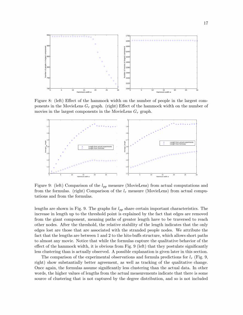
Figure 10: (left) Calibrating the value of ε in the synthetic model of EachMovie producesdatasets with required specifications on minimum rating κ. (right) Comparison of the lppmeasure (EachMovie) from actual computations and from the formulas for varying values ofκ.

in the formulas.

4.2.2 EachMovie

The evaluation of the EachMovie data is more difficult owing to inconsistencies in datacollection. For example, the dataset was collected in two phases, with entirely differentrating instructions and scales in the two situations, and also contains duplicate ratings. Weconcentrate on the portion of the data collected in 1997 and use a synthetic dataset that hasthe same sparsity and exponent of the power-law as this reduced dataset. Specifically, ourdataset includes 500 people and 75 movies and has the property that the person with buffindex b has seen the first d75b−εe movies (recall that the movies are also ordered accordingto their hit id). An ε = 0.7 produces a dataset with a minimum rating of 1 movie (95.5%sparse), while ε = 0.27 produces a minimum rating of 15 movies (with sparsity 76.63%).The choice of ε thus provides a systematic way to analyze the effect of the minimum ratingconstraint κ (see Fig. 10, left). In addition, for each (person, movie) edge of these syntheticgraphs, we generate a uniform (discrete) random variate in [0, 10] and rewire the movieendpoint of the edge if this variate is < 2. This device models deviations from a stricthits-buffs distribution. We generated 15 such graphs and ensured that they were connected(in some cases, manual changes were made to ensure that the graph was connected). Thesegraphs served as the starting points for our analysis. For each of these 15 graphs, we vary thehammock width w from 1 to 25 and repeat the length calculations (using both experimentsand formula predictions) for the social network and recommender graphs.

Like the MovieLens experiment, the formulas for EachMovie predict shorter lpp lengths(and consequently, lesser clustering) than observed from actual experiments. To characterizethe mismatch, for each of the 15 values of κ, we express the differences between the formulapredictions and experimental observations as a vector (of length 25, for each of the 25 valuesof hammock width w). The L∞ norm of this vector is plotted against κ in Fig. 10 (right).Notice the relatively linear growth of the discrepancy as κ increases. In the range of κconsidered, the hammock constraints shatter the graph into many small components, so

19

0 5 10 15 20 251

1.5

2

2.5

3

3.5

4

4.5

Hammock width w

Ave

rage

l r leng

th

Length from actual experimentsLength from formulas

0 5 10 15 20 251

1.1

1.2

1.3

1.4

1.5

1.6

1.7

1.8

Hammock width w

Ave

rage

l r leng

th

Length from actual experimentsLength from formulas

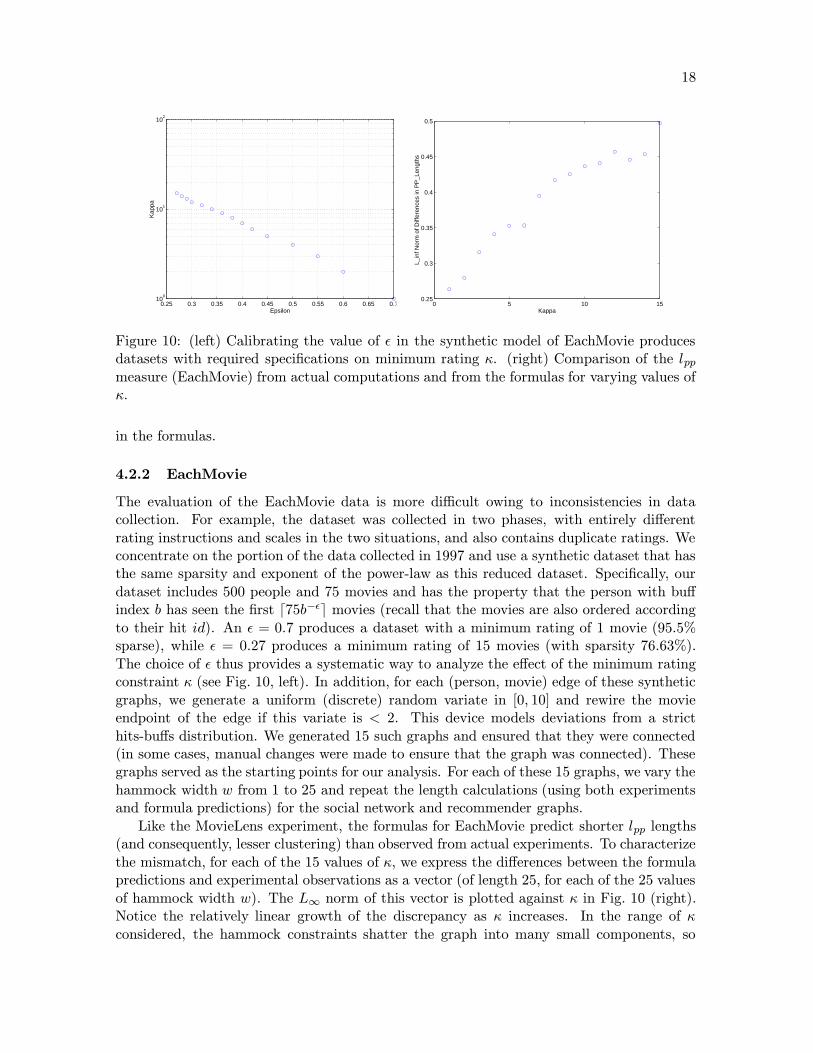
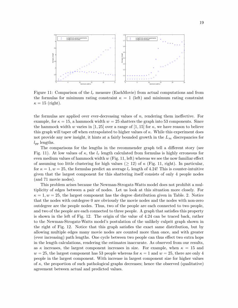
Figure 11: Comparison of the lr measure (EachMovie) from actual computations and fromthe formulas for minimum rating constraint κ = 1 (left) and minimum rating constraintκ = 15 (right).

the formulas are applied over ever-decreasing values of n, rendering them ineffective. Forexample, for κ = 15, a hammock width w = 25 shatters the graph into 53 components. Sincethe hammock width w varies in [1, 25] over a range of [1, 15] for κ, we have reason to believethis graph will taper off when extrapolated to higher values of κ. While this experiment doesnot provide any new insight, it hints at a fairly bounded growth in the L∞ discrepancies forlpp lengths.

The comparisons for the lengths in the recommender graph tell a different story (seeFig. 11). At low values of κ, the lr length calculated from formulas is highly erroneous foreven medium values of hammock width w (Fig. 11, left) whereas we see the now familiar effectof assuming too little clustering for high values (≥ 12) of κ (Fig. 11, right). In particular,for κ = 1, w = 25, the formulas predict an average lr length of 4.24! This is counter-intuitivegiven that the largest component for this shattering itself consists of only 4 people nodes(and 71 movie nodes).

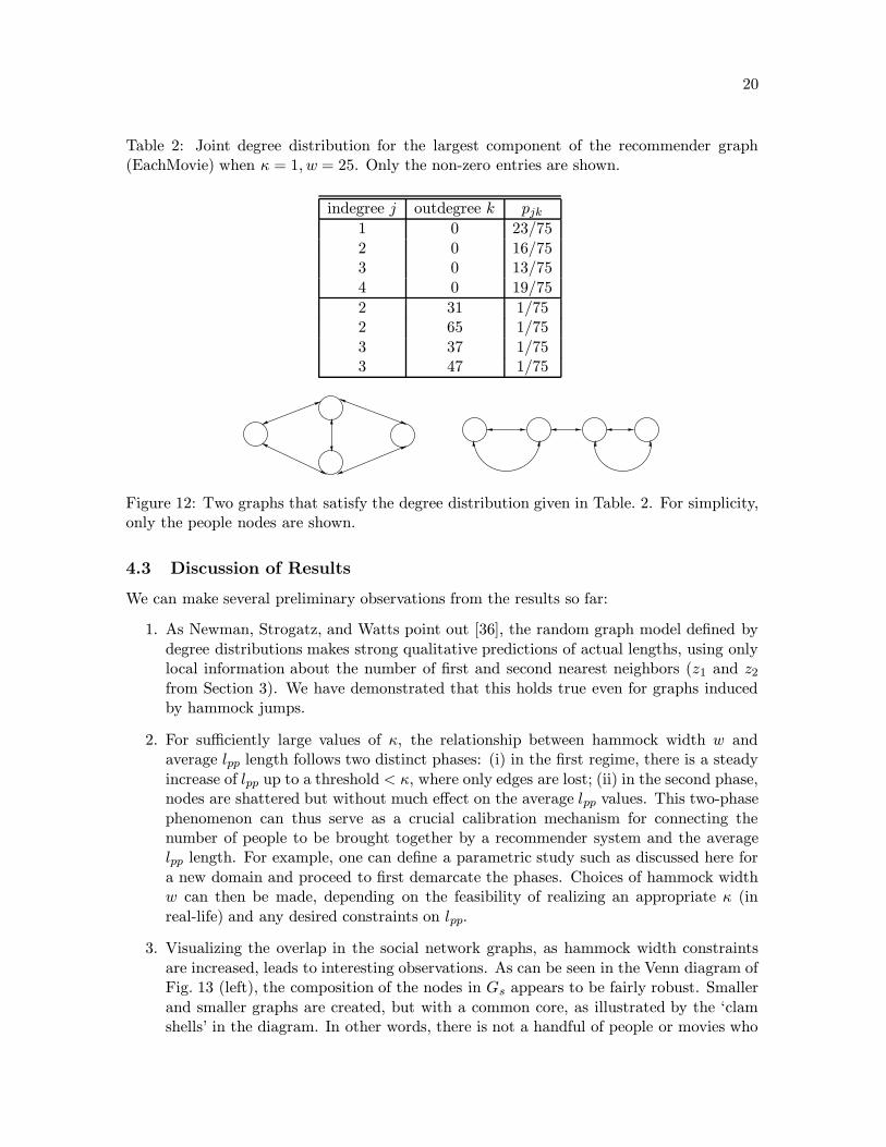
This problem arises because the Newman-Strogatz-Watts model does not prohibit a mul-tiplicity of edges between a pair of nodes. Let us look at this situation more closely. Forκ = 1, w = 25, the largest component has the degree distribution given in Table. 2. Noticethat the nodes with outdegree 0 are obviously the movie nodes and the nodes with non-zerooutdegree are the people nodes. Thus, two of the people are each connected to two people,and two of the people are each connected to three people. A graph that satisfies this propertyis shown in the left of Fig. 12. The origin of the value of 4.24 can be traced back, ratherto the Newman-Strogatz-Watts model’s postulation of the unlikely culprit graph shown inthe right of Fig. 12. Notice that this graph satisfies the exact same distribution, but byallowing multiple edges many movie nodes are counted more than once, and with greater(ever increasing) path lengths. One cycle between two people can thus effect two extra hopsin the length calculations, rendering the estimates inaccurate. As observed from our results,as κ increases, the largest component increases in size. For example, when κ = 15 andw = 25, the largest component has 53 people whereas for κ = 1 and w = 25, there are only 4people in the largest component. With increase in largest component size for higher valuesof κ, the proportion of such pathological graphs decreases; hence the observed (qualitative)agreement between actual and predicted values.

20

Table 2: Joint degree distribution for the largest component of the recommender graph(EachMovie) when κ = 1, w = 25. Only the non-zero entries are shown.

indegree j outdegree k pjk1 0 23/752 0 16/753 0 13/754 0 19/75

2 31 1/752 65 1/753 37 1/753 47 1/75

Figure 12: Two graphs that satisfy the degree distribution given in Table. 2. For simplicity,only the people nodes are shown.

4.3 Discussion of Results

We can make several preliminary observations from the results so far:

1. As Newman, Strogatz, and Watts point out [36], the random graph model defined bydegree distributions makes strong qualitative predictions of actual lengths, using onlylocal information about the number of first and second nearest neighbors (z1 and z2

from Section 3). We have demonstrated that this holds true even for graphs inducedby hammock jumps.

2. For sufficiently large values of κ, the relationship between hammock width w andaverage lpp length follows two distinct phases: (i) in the first regime, there is a steadyincrease of lpp up to a threshold < κ, where only edges are lost; (ii) in the second phase,nodes are shattered but without much effect on the average lpp values. This two-phasephenomenon can thus serve as a crucial calibration mechanism for connecting thenumber of people to be brought together by a recommender system and the averagelpp length. For example, one can define a parametric study such as discussed here fora new domain and proceed to first demarcate the phases. Choices of hammock widthw can then be made, depending on the feasibility of realizing an appropriate κ (inreal-life) and any desired constraints on lpp.

3. Visualizing the overlap in the social network graphs, as hammock width constraintsare increased, leads to interesting observations. As can be seen in the Venn diagram ofFig. 13 (left), the composition of the nodes in Gs appears to be fairly robust. Smallerand smaller graphs are created, but with a common core, as illustrated by the ‘clamshells’ in the diagram. In other words, there is not a handful of people or movies who

21

Figure 13: (left) ‘Clam shells’ view of the social networks Gs induced by various hammockwidths. Increasing hammock width leads to smaller networks. (right) a hypothetical situa-tion likely to be caused by the presence of a few strong points in the graph.

form a cutset for the graph — there is no small group of people or movies whose removal(by a sufficiently strict hammock width) causes the entire graph to be broken into twoor more pieces (see right of Fig. 13). This confirms observations made elsewhere [6] thatpower-laws are a major factor ensuring the robustness and scaling properties of graph-based networks. Our study is the first to investigate this property for graphs inducedby hammock jumps. However, we believe this robustness is due to the homogeneousnature of ratings in the movie domain. In other domains such as music CDs, wherepeople can be partitioned by preference, the diagram on the right of Fig. 13 would bemore common.

4. The average lr lengths are within the range [1, 2] in both formula predictions andexperimental results. Caution has to be exercised whenever the graph size n getssmall, as Fig. 12 shows. In our case, this happens when the hammock width constraintw rises above the minimum rating constraint κ. Of course, this behavior should alsobe observed for other strict jumps.

5. Both of the lpp and lr formulas postulate consistently less clustering than observed inthe real data. We attempt to address this below. The typical random graph modelhas a Poisson distribution of edges [9], whereas, as seen earlier, real datasets exhibit apower-law distribution [13, 16]. The power-law feature is sometimes described as ‘scale-free’ or ‘scale-invariant’ since a single parameter (the exponent of the law) capturesthe size of the system at all stages in its cycle (the x-axis of the law). A log-log plotof values would thus produce a straight line, an effect not achievable by traditionalrandom graph models. Barabasi and Albert [6] provide two sufficient conditions forthis property: growth and preferential attachment. Growth refers to the ability of thesystem to dynamically add nodes; random graph models that fix the number of nodesare unable to expand. Preferential attachment refers to the phenomenon that nodesthat have high degrees have a greater propensity of being linked to by new nodes.In our case, a movie that is adjudged well by most people is likely to become a hitwhen additional people are introduced. Barabasi and Albert refer to this as a “richget richer” effect [6].

22

0 100 200 300 400 500 600 700 800 900 10000

0.2

0.4

0.6

0.8

1

1.2

Degree d

P[D

>=

d]

0 0.2 0.4 0.6 0.8 1 1.2 1.4 1.6 1.8 2

x 104

0

0.2

0.4

0.6

0.8

1

1.2

Degree d

P[D

>=

d]

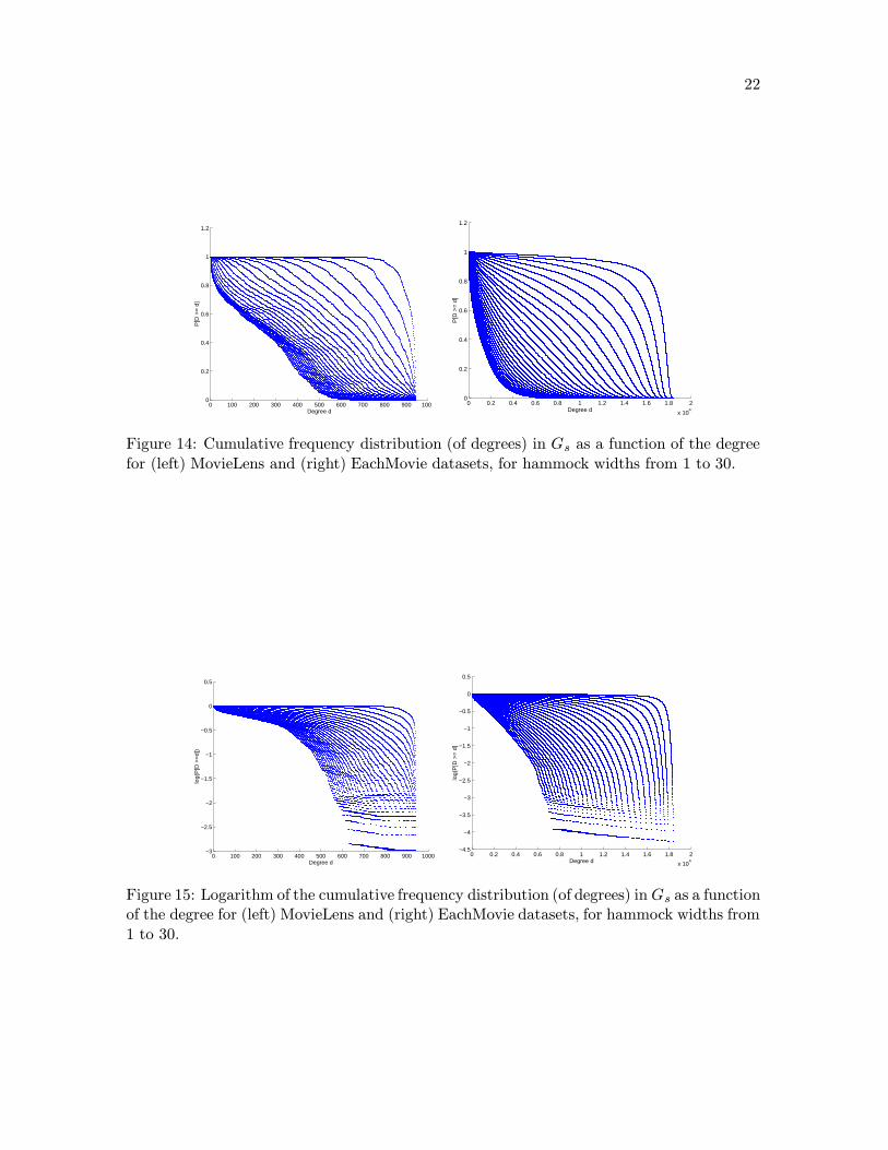
Figure 14: Cumulative frequency distribution (of degrees) in Gs as a function of the degreefor (left) MovieLens and (right) EachMovie datasets, for hammock widths from 1 to 30.

0 100 200 300 400 500 600 700 800 900 1000−3

−2.5

−2

−1.5

−1

−0.5

0

0.5

Degree d

log(

P[D

>=

d])

0 0.2 0.4 0.6 0.8 1 1.2 1.4 1.6 1.8 2

x 104

−4.5

−4

−3.5

−3

−2.5

−2

−1.5

−1

−0.5

0

0.5

Degree d

log(

P[D

>=

d]

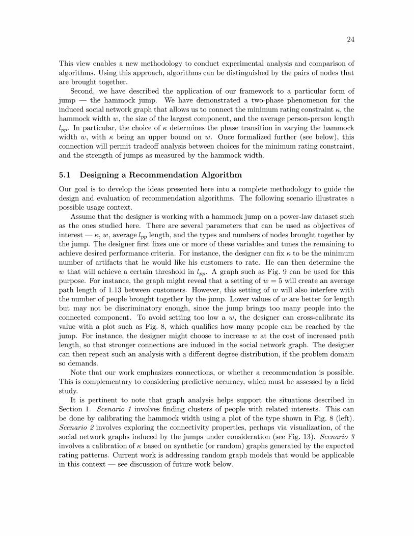
Figure 15: Logarithm of the cumulative frequency distribution (of degrees) in Gs as a functionof the degree for (left) MovieLens and (right) EachMovie datasets, for hammock widths from1 to 30.

23

To characterize the possible causes in our domain, we consider the distribution ofdegrees in the social network graphs Gs of both MovieLens and (the actual) EachMoviedatasets (see Fig. 14). In the figure, lines from top to bottom indicate increasinghammock widths. Both datasets do not follow a strict power law for the entire rangeof the hammock width w. For low values of w, there is a small and steadily increasingpower-law regime, followed by an exponential cutoff. For higher values of w, the graph‘falls’ progressively earlier and the CDF resembles a Gaussian or exponential decay,with no power-law behavior. This is evident if the logarithm of the CDF is plotted,as in Fig. 15 where top to bottom indicates increasing hammock widths. Notice thesignificant cusp in the left side of both graphs, depicting the qualitative change inbehavior. These two extremes of deviations from power-law behavior (at low andhigh values of w) are referred to as broad-scale and single-scale [4], respectively, todistinguish them from the scale-free behavior of power-laws.

Causes for such deviations from a pure power-law are also understood, e.g. agingand capacity. Aging refers to the fact that after a certain point in time, nodes stopaccumulating edges. Capacity refers to resource-bounded environments where cost andeconomics prevent the hits from becoming arbitrarily greater hits. These observationshave been verified for environments such as airports (capacity limitations on runways),and natural networks (aging caused by people dying) [4].

In our domain, recall that the Gs graphs model the connectivities among people, andare hence indirect observations from an underlying bipartite graph. One possible ex-planation for the deviations of the connectivities in Gs from from power-law behavioris suggested in a study done by Robalino and Gibney [45], which models the impactof movie demand on the social network underlying a word-of-mouth recommendation.The two new factors introduced there are expectation and homogeneity (of the socialnetwork). The authors suggest that “some movies might end up having low demand,depending on the initial agents expectations and their propagation through the socialnetwork” [45]. Furthermore, they assume that negative information (ratings) obtainedearly in a movie’s lifetime can have substantial effect in a homogeneous network (onewhere individuals trust each others opinions strongly than in other networks). At thispoint, we are unable to accept or reject this observation due to lack of informationabout the social dynamics in which the data was collected in MovieLens and Each-Movie.

However, such an effect might not still model the shift in the emphasis from a broad-scale behavior to a single-scale behavior as w increases. Fortunately, this is easy toexplain algorithmically from our construction. For higher values of w, the degreedistributions resemble more and more a typical random graph (for smaller values ofn), which has a connectivity characterized by a fast decaying tail (such as a Poissondistribution). Insisting on greater values of w leads to higher and higher decays, suchthat for sufficiently large w (relative to κ), no power-law regime is visible [4].

5 Concluding Remarks

This research makes two key contributions. First, we have shown how algorithms for recom-mender systems can be studied in terms of the connections they make in a bipartite graph.

24

This view enables a new methodology to conduct experimental analysis and comparison ofalgorithms. Using this approach, algorithms can be distinguished by the pairs of nodes thatare brought together.

Second, we have described the application of our framework to a particular form ofjump — the hammock jump. We have demonstrated a two-phase phenomenon for theinduced social network graph that allows us to connect the minimum rating constraint κ, thehammock width w, the size of the largest component, and the average person-person lengthlpp. In particular, the choice of κ determines the phase transition in varying the hammockwidth w, with κ being an upper bound on w. Once formalized further (see below), thisconnection will permit tradeoff analysis between choices for the minimum rating constraint,and the strength of jumps as measured by the hammock width.

5.1 Designing a Recommendation Algorithm

Our goal is to develop the ideas presented here into a complete methodology to guide thedesign and evaluation of recommendation algorithms. The following scenario illustrates apossible usage context.

Assume that the designer is working with a hammock jump on a power-law dataset suchas the ones studied here. There are several parameters that can be used as objectives ofinterest — κ, w, average lpp length, and the types and numbers of nodes brought together bythe jump. The designer first fixes one or more of these variables and tunes the remaining toachieve desired performance criteria. For instance, the designer can fix κ to be the minimumnumber of artifacts that he would like his customers to rate. He can then determine thew that will achieve a certain threshold in lpp. A graph such as Fig. 9 can be used for thispurpose. For instance, the graph might reveal that a setting of w = 5 will create an averagepath length of 1.13 between customers. However, this setting of w will also interfere withthe number of people brought together by the jump. Lower values of w are better for lengthbut may not be discriminatory enough, since the jump brings too many people into theconnected component. To avoid setting too low a w, the designer can cross-calibrate itsvalue with a plot such as Fig. 8, which qualifies how many people can be reached by thejump. For instance, the designer might choose to increase w at the cost of increased pathlength, so that stronger connections are induced in the social network graph. The designercan then repeat such an analysis with a different degree distribution, if the problem domainso demands.

Note that our work emphasizes connections, or whether a recommendation is possible.This is complementary to considering predictive accuracy, which must be assessed by a fieldstudy.

It is pertinent to note that graph analysis helps support the situations described inSection 1. Scenario 1 involves finding clusters of people with related interests. This canbe done by calibrating the hammock width using a plot of the type shown in Fig. 8 (left).Scenario 2 involves exploring the connectivity properties, perhaps via visualization, of thesocial network graphs induced by the jumps under consideration (see Fig. 13). Scenario 3involves a calibration of κ based on synthetic (or random) graphs generated by the expectedrating patterns. Current work is addressing random graph models that would be applicablein this context — see discussion of future work below.

25

Small−World network modelHits−Buffs rewiring model

0 0.1 0.2 0.3 0.4 0.5 0.6 0.7 0.8 0.9 12

4

6

8

10

12

14

16

18

Probability (p)

Ave

rage

Len

gth

Ratings

0200

400600

8001000

0

500

1000

1500

20001

2

3

4

5

MOVIESPEOPLE

RA

TIN

GS

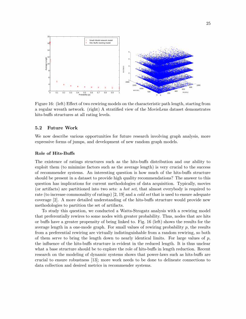
Figure 16: (left) Effect of two rewiring models on the characteristic path length, starting froma regular wreath network. (right) A stratified view of the MovieLens dataset demonstrateshits-buffs structures at all rating levels.

5.2 Future Work

We now describe various opportunities for future research involving graph analysis, moreexpressive forms of jumps, and development of new random graph models.

Role of Hits-Buffs

The existence of ratings structures such as the hits-buffs distribution and our ability toexploit them (to minimize factors such as the average length) is very crucial to the successof recommender systems. An interesting question is how much of the hits-buffs structureshould be present in a dataset to provide high quality recommendations? The answer to thisquestion has implications for current methodologies of data acquisition. Typically, movies(or artifacts) are partitioned into two sets: a hot set, that almost everybody is required torate (to increase commonality of ratings) [2, 19] and a cold set that is used to ensure adequatecoverage [2]. A more detailed understanding of the hits-buffs structure would provide newmethodologies to partition the set of artifacts.

To study this question, we conducted a Watts-Strogatz analysis with a rewiring modelthat preferentially rewires to some nodes with greater probability. Thus, nodes that are hitsor buffs have a greater propensity of being linked to. Fig. 16 (left) shows the results for theaverage length in a one-mode graph. For small values of rewiring probability p, the resultsfrom a preferential rewiring are virtually indistinguishable from a random rewiring, so bothof them serve to bring the length down to nearly identical limits. For large values of p,the influence of the hits-buffs structure is evident in the reduced length. It is thus unclearwhat a base structure should be to explore the role of hits-buffs in length reduction. Recentresearch on the modeling of dynamic systems shows that power-laws such as hits-buffs arecrucial to ensure robustness [13]; more work needs to be done to delineate connections todata collection and desired metrics in recommender systems.

26

Expressive Jumps

Our experimentation has concentrated on the hammock jump varied by the hammock widthparameter. However, it is also possible to consider other jumps within this framework,and compare them by the connections they make for the same recommender dataset. Thiscomparison can concentrate on the clusters of people (or people and movies) that are broughttogether (illustrated in Fig. 13). For instance, given two algorithms A and B parameterizedby α, we would be able to make statements of the form

Algorithm A with α = 2 makes the same connections as algorithm B with α ≤ 6.

Results of this form would aid in the selection of recommendation algorithms by the relativestrengths of the underlying jump.

This approach would clearly point us in the direction of trying to find algorithms thatuse the strongest jump possible for all datasets. However, these algorithms may be compu-tationally intensive (for instance, recently proposed algorithms that use mixture models [22]and latent variables [25]), while in a particular dataset the jump is actually equivalent to oneperformed by a much less expensive algorithm. This point is illustrated by the observationin our experimentation that the path lengths in the recommender graph are between 1 and2, which suggests that algorithms that attempt to find longer paths will end up being equiv-alent to algorithms that do not. Therefore, the choice of algorithm is strongly dependenton the dataset, and simpler machinery may be more efficient and cost effective than morecomplex algorithms that would perform better in other contexts.

The need to identify efficient forms of jumping is more important when additional in-formation, such as rating values, is included in jump calculations. Fig. 16 (right) showsthe ratings information present in the MovieLens dataset. As can be seen, the hits-buffsstructure is stratified by rating values into multiple layers and can be used advantageouslyboth within a ratings layer and across layers. Algorithms can exploit such prior knowledgeof rating patterns to make cheaper jumps.

Finally, we make the observation that almost always, recommendation algorithms neverbring disconnected portions of a graph together, and when they do, it is in only very patho-logical cases. This observation, in part, leads us to the belief that all recommender jumpsdepend in some way on hammock jumps. In some cases this dependency is obvious, butothers will require more study.

New Random Graph Models

The formulas presented in this paper for the lengths of the social network graph and of therecommender graph are derived from the parameters of the induced Gs and Gr graphs. Onepossible direction of work is to cast these variables in terms of parameters of the originalbipartite graph (or datasetR). However, the Newman-Strogatz-Watts model is very difficultto analyze for all but the simplest forms of jumps. Recall the Aiello-Chung-Lu model [3] formassive graphs modeled after power-laws. Unlike the Newman-Strogatz-Watts model andlike traditional random graph models, this model has only two parameters (the interceptand slope of the power-law plotted on a log-log scale). Estimations of graph properties suchas diameter have very recently been initiated [34] for this new model and it appears to be apromising candidate for application to recommender systems. In particular, we could aim fora more accurate modeling of the connection between κ and the hammock width constraint

27

w at which the graph becomes shattered.

Acknowledgements: The authors express their thanks to L.S. Heath for helpful discussions.Acknowledgements are also due to the Compaq Equipment Corporation, which provided theEachMovie dataset and the University of Minnesota, which provided the MovieLens datasetused in our experiments.

References

[1] L.A. Adamic. “The Small World Web”. In ECDL’99, Proceedings of the Third EuropeanConference on Research and Advanced Technology for Digital Libraries, pages 443–452.Springer-Verlag, 1999.

[2] C.C. Aggarwal, J.L. Wolf, K.-L. Wu, and P.S. Yu. “Horting Hatches an Egg: A NewGraph-Theoretic Approach to Collaborative Filtering”. In KDD’99, Proceedings ofthe Fifth ACM SIGKDD International Conference on Knowledge Discovery and DataMining, pages 201–212. ACM Press, 1999.

[3] W. Aiello, F. Chung, and L. Lu. “A Random Graph Model for Massive Graphs”. InSTOC’00, Proceedings of the ACM Symposium on Theory of Computing, pages 171–180.ACM Press, 2000.

[4] L.N. Amaral, A. Scala, M. Bathelemy, and H.E. Stanley. “Classes of Behavior of Small-World Networks”. Proceedings of the National Academy of Science, USA, Vol. 97:pages11149–11152, 2000.

[5] C. Avery and R. Zeckhauser. “Recommender Systems for Evaluating Computer Mes-sages”. Communications of the ACM, Vol. 40(3):pages 88–89, March 1997.

[6] A.-L. Barabasi and R. Albert. “Emergence of Scaling in Random Networks”. Science,Vol. 286:pages 509–512, October 1999.

[7] C. Basu, H. Hirsh, and W.W. Cohen. “Recommendation as Classification: Using Socialand Content-Based Information in Recommendation”. In AAAI’98, Proceedings of theFifteeth National Conference on Artifical Intelligence, pages 714–720. AAAI Press, 1998.

[8] D. Billsus and M. Pazzani. “Learning Collaborative Information Filters”. In ICML’98,Proceedings of the Fifteenth International Conference on Machine Learning, pages 46–53. Morgan Kaufmann, 1998.

[9] B. Bollabas. “Random Graphs”. Academic Press, London, 1985.

[10] J.S. Breese, D. Heckerman, and C. Kadie. “Empirical Analysis of Predictive Algo-rithms for Collaborative Filtering”. In UAI’98, Proceedings of the Fourteenth AnnualConference on Uncertainty in Artificial Intelligence, pages 43–52. Morgan Kaufmann,1998.

[11] S. Brin and L. Page. “The Anatomy of a Large-Scale Hypertextual Web Search Engine”.In WWW’98, Proceedings of the Seventh International World Wide Web Conference,pages 107–117. Elsevier Science, 1998.

28

[12] A. Broder, R. Kumar, F. Maghoul, P. Raghavan, S. Rajagopalan, R. Stata, A. Tomkins,and J. Wiener. “Graph Structure in the Web”. In WWW’99, Proceedings of the NinthInternational World Wide Web Conference, 1999.

[13] J.M. Carlson and J. Doyle. “Highly Optimized Tolerance: A Mechanism for Power Lawsin Designed Systems”. Physical Review, E60(1412), 1999.

[14] S. Chakrabarti, B.E. Dom, S. Ravi Kumar, P. Raghavan, S. Rajagopalan, A. Tomkins,D. Gibson, and J. Klienberg. “Mining the Web’s Link Structure”. IEEE Computer,Vol. 32(8):pages 60–67, August 1999.

[15] P. Erdos and A. Renyi. “On Random Graphs”. Publicationes Mathematicae, Vol. 6:pages290–297, 1959.

[16] M. Faloutsos, P. Faloutsos, and C. Faloutsos. “On Power-Law Relationships of theInternet Topology”. In Proceedings of the ACM SIGCOM Conference on Applications,Technologies, Architectures, and Protocols for Computer Communication, pages 251–262. ACM Press, 1999.

[17] G.W. Flake, S. Lawrence, and C. Lee Giles. “Efficient Identification of Web Commu-nities”. In KDD’00, Proceedings of the Sixth ACM SIGKDD International Conferenceon Knowledge Discovery and Data Mining, pages 150–160. ACM Press, 2000.

[18] D. Gibson, J. Kleinberg, and P. Raghavan. “Clustering Categorical Data: An ApproachBased on Dynamical Systems”. VLDB Journal, Vol. 8(3-4):pages 222–236, 2000.

[19] K. Goldberg, T. Roeder, D. Gupta, and C. Perkins. “Eigentaste: A Constant TimeCollaborative Filtering Algorithm”. Technical Report M00/41, Electronic ResearchLaboratory, University of Berkeley, August 2000.

[20] N. Good, J. Scafer, J. Konstan, A. Borchers, B. Sarwar, J. Herlocker, and J. Riedl.“Combining Collaborative Filtering with Personal Agents for Better Recommenda-tions”. In AAAI’99, Proceedings of the Sixteenth National Conference on ArtificalIntelligence, pages 439–446. AAAI Press, 1999.

[21] L.S. Heath. Personal Communication, 2001.

[22] D. Heckerman, D.M. Chickering, C. Meek, R. Rounthwaite, and C. Kadie. “DependencyNetworks for Inference, Collaborative Filtering, and Data Visualization”. Journal ofMachine Learning Research, Vol. 1:pages 49–75, 2000.

[23] J. Herlocker, J. Konstan, A. Borchers, and J. Riedl. “An Algorithmic Framework forPerforming Collaborative Filtering”. In SIGIR’99, Proceedings of the Twenty SecondAnnual ACM Conference on Research and Development in Information Retrieval, pages230–237. ACM Press, 1999.

[24] W. Hill, L. Stead, M. Rosenstein, and G. Furnas. “Recommending and EvaluatingChoices in a Virtual Community of Use”. In CHI’95, Proceedings of the ACM Conferenceon Human Factors and Computing Systems, pages 194–201. ACM Press, 1995.

29

[25] T. Hofmann and J. Puzicha. “Latent Class Models for Collaborative Filtering”. InIJCAI’99, Proceedings of the 16th International Joint Conference on Artificial intelli-gence. IJCAI Press, 1999.

[26] H. Kautz, B. Selman, and M. Shah. “ReferralWeb: Combining Social Networks andCollaborative Filtering”. Communications of the ACM, Vol. 40(3):pages 63–65, March1997.

[27] B. Kitts, D. Freed, and M. Vrieze. “Cross-Sell: A Fast Promotion-Tunable Customer-Item Recommendation Method Based on Conditional Independent Probabilities”. InKDD’00, Proceedings of the Sixth International Conference on Knowledge Discoveryand Data Mining, pages 437–446. ACM Press, 2000.

[28] J. Kleinberg. “Authoritative Sources in a Hyperlinked Environment”. Journal of theACM, Vol. 46(5):pages 604–632, September 1999.

[29] J. Kleinberg. “The Small-World Phenomenon: An Algorithmic Perspective”. Nature,Vol. 406(6798), August 2000.

[30] A. Kohrs and B. Merialdo. “Clustering for Collaborative Filtering Applications”. InProceedings of Computational Intelligence for Modelling, Control and Automation. IOSPress, 1999.

[31] J. Konstan, B. Miller, D. Maltz, J. Herlocker, L. Gordan, and J. Riedl. “GroupLens:Applying Collaborative Filtering to Usenet News”. Communications of the ACM, Vol.40(3):pages 77–87, March 1997.

[32] R. Kumar, P. Raghavan, S. Rajagopalan, and A. Tomkins. “Trawling the Web forEmerging Cyber-Communities”. In WWW’99, Proceedings of the Eighth InternationalWorld Wide Web Conference, 1999.

[33] Macromedia LikeMinds. “Macromedia LikeMinds Personalization and Performance”.URL: http://ebusiness.macromedia.com/software/likeminds/whitepapers/lm

white 3rd.pdf.

[34] L. Lu. “The Diameter of Random Massive Graphs”. In SODA’00, Proceedings ofthe Twelth Annual ACM-SIAM Symposium on Discrete Algorithms, pages 912–921.ACM/SIAM Press, 2000.

[35] B.J. Mirza. “Jumping Connections: A Graph-Theoretic Model for Recommender Sys-tems”. Master’s thesis, Virginia Tech, February 2001. 64 pages.

[36] M. Newman, S. Strogatz, and D. Watts. “Random Graphs with Arbitrary DegreeDistribution and their Applications”. Technical Report 0007042, Santa Fe Institute,2000.

[37] M. O’Conner and J. Herlocker. “Clustering Items for Collaborative Filtering”. InProceedings of the ACM SIGIR Workshop on Recommender Systems, 1999.

[38] D. Payton. “Discovering Collaborators by Analyzing Trails through an InformationSpace”. In Proceedings of the AAAI Fall Symposium on Artificial Intelligence and LinkAnalysis, pages 84–87. AAAI Press, 1998.

30

[39] D. Pennock, E. Horvitz, S. Lawrence, and C. Giles. “Collaborative Filtering by Person-ality Diagnosis: A Hybrid Memory- and Model-Based Approach”. In UAI’00, Proceed-ings of the Sixteenth Conference on Uncertainty in Artificial Intelligence, pages 473–480.Morgan Kaufmann, 2000.

[40] P. Pirolli, J. Pitkow, and R. Rao. “Silk from a Sow’s Ear: Extracting Usable Structuresfrom the Web”. In CHI’96, Proceedings of the ACM Conference on Human Factors andComputing Systems. ACM Press, 1996.

[41] P. Resnick and H. Varian. “Recommender Systems”. Communications of the ACM,Vol. 40(3):pages 56–58, March 1997.

[42] L. Richard. “Automatic Information Extraction from Documents: A Tool for Intelli-gence and Law Enforcement Analysts”. In Proceedings of the AAAI Fall Symposium onArtificial Intelligence and Link Analysis, pages 63–67. AAAI Press, 1998.

[43] J. Riedl and J. Konstan. “GroupLens Research”. URL: http://www.cs.umn.edu/

Research/GroupLens/.

[44] E. Riloff and L. Hollaar. “Text Databases and Information Retrieval”. In A.B.Tucker Jr., editor, “The Computer Science and Engineering Handbook”, pages 1125–1141. CRC Press, 1996.

[45] D. Robalino and M. Gibney. “A Model of the Impact on Movie Demand of SocialNetworks and Word of Mouth Recommendation”. URL: http://www.metaculture.

net/Searches/movies, 1999.

[46] B. Sarwar, G. Karypis, J. Konstan, and J. Riedl. “Analysis of Recommendation Algo-rithms for E-Commerce”. In Proceedings of the Second ACM Conference on ElectronicCommerce, pages 158–167. ACM Press, 2000.

[47] B. Sarwar, G. Karypis, J. Konstan, and J. Riedl. “Application of Dimensionality Re-duction in Recommender System – A Case Study”. Technical Report CS-TR 00-043,Computer Science and Engineering Dept., University of Minnesota, July 2000.

[48] J. Schafer, J. Konstan, and J. Riedl. “Recommender Systems in E-Commerce”. InProceedings of the First ACM Conference on Electronic Commerce, pages 158–166. ACMPress, 1999.

[49] M.F. Schwartz and D.C.M. Wood. “Discovering Shared Interests Using Graph Analy-sis”. Communications of the ACM, Vol. 36(8):pages 78–89, August 1993.

[50] U. Shardanand and P. Maes. “Social Information Filtering: Algorithms for Automating‘Word of Mouth’”. In CHI’95, Proceedings of the ACM Conference on Human Factorsand Computing Systems, pages 210–217. ACM Press, 1995.

[51] I. Soboroff and C. Nicholas. “Combining Content and Collaboration in Text Filtering”.In Proceedings of the IJCAI’99 Workshop on Machine Learning in Information Filtering,pages 86–91, 1999.

31

[52] D. Swanson and N. Smalheiser. “Link Analysis of MedLine Titles as an Aid to ScientificDiscovery”. In Proceedings of the AAAI Fall Symposium on Artificial Intelligence andLink Analysis, pages 94–97. AAAI Press, 1998.

[53] L. Terveen, W. Hill, B. Amento, D. McDonald, and J. Creter. “PHOAKS: A Systemfor Sharing Recommendations”. Communications of the ACM, Vol. 40(3):pages 59–62,March 1997.

[54] L. Ungar and D. Foster. “Clustering Methods for Collaborative Filtering”. In Proceed-ings of the AAAI-98 Workshop on Recommender Systems, pages 112–125. AAAI Press,1998.

[55] S. Wasserman and K. Faust. “Social Network Analysis: Methods and Applications”.Cambridge University Press, New York, 1994.

[56] D. Watts and S. Strogatz. “Collective Dynamics of ‘Small-World’ Networks”. Nature,Vol. 393(6):pages 440–442, June 1998.