Analysis Tool for Model Output to Evaluate Express Toll Lanes Feasibility

STUDY TO EVALUATE THE ECONOMIC FEASIBILITY OF REPLACING A
PRESSURE REDUCING VALVE WITH A PRESSURE REDUCING TURBINE
FOR A SPECIFIC CASE STUDY
Francis Joseph Nadaraju
A Research Report submitted to the Faculty of Engineering and the Built
Environment, University of the Witwatersrand, in partial fulfilment of the
requirements for the Master of Science in Engineering.
Johannesburg, 2011

TABLE OF CONTENTS
DECLARATION........................................ ............................................................ i
ABSTRACT........................................... .............................................................. ii
ACKNOWLEDGEMENTS ................................... ............................................... iii
LIST OF FIGURES ............................................................................................. iv
LIST OF TABLES..................................... .......................................................... vi
LIST OF SYMBOLS .................................... ...................................................... vii
1 INTRODUCTION ...................................................................................... 1
1.1 Energy recovery.................................... .................................................. 4
1.2 Plan of development................................ ............................................... 7
2 LITERATURE REVIEW .................................. .......................................... 9
2.1 Energy recovery in mining applications ............. .................................. 9
2.2 Pumps as turbines.................................. .............................................. 15
2.3 Applications of pump-turbine systems ............... ................................ 16
2.4 Conclusion ......................................... ................................................... 19
3 THEORETICAL BACKGROUND ............................. .............................. 20
3.1 First law of thermodynamics ........................ ....................................... 20
3.2 Flow processes..................................... ................................................ 21
3.3 Second law of thermodynamics ....................... ................................... 23
3.3.1 Heat engines........................................................................................... 24
3.3.2 Entropy ................................................................................................... 27
3.4 Property relationships............................. ............................................. 29
3.4.1 Internal energy and enthalpy................................................................... 29
3.4.2 Enthalpy and entropy.............................................................................. 29
3.4.3 Specific volume....................................................................................... 31
3.4.4 Joule-Thomson effect ............................................................................. 31
3.5 Turbine expansion process .......................... ....................................... 32
3.6 Mechanical energy balance.......................... ........................................ 35
3.7 Frictional losses .................................. ................................................. 36
3.7.1 Pipe friction............................................................................................. 36
3.7.2 Other frictional losses ............................................................................. 38
3.8 System characteristic.............................. ............................................. 39

3.9 Electrical generators .............................. .............................................. 40
3.9.1 Electrical drives....................................................................................... 41
3.9.2 Operating speed ..................................................................................... 43
3.10 Conclusion ......................................... ................................................... 44
4 DISCUSSION ......................................................................................... 45
4.1 Anglogold Ashanti Mponeng mine (du Toit, 2009) ..... ........................ 45
4.2 Design criteria.................................... ................................................... 48
4.2.1 Water flow and pressure data ................................................................. 48
4.2.2 Regression of water flow and pressure data ........................................... 49
4.2.3 Water temperature.................................................................................. 54
4.2.4 Heat capacity.......................................................................................... 55
4.2.5 Specific volume and density.................................................................... 56
4.2.6 Viscosity ................................................................................................. 57
4.2.7 Joule-Thomson coefficient ...................................................................... 58
4.2.8 Summary of design criteria ..................................................................... 59
4.3 System modelling ................................... .............................................. 59
4.3.1 System curve.......................................................................................... 59
4.3.2 Pump-turbine model................................................................................ 61
4.3.3 System alternatives: variable and constant speed operation................... 64
4.3.4 Energy recovery and discharge water temperature................................. 73
4.3.5 Electrical design...................................................................................... 74
4.3.6 System operation and control ................................................................. 79
4.4 Capital expenditure................................ ............................................... 83
4.5 Financial analysis ................................. ................................................ 83
4.5.1 Net present value and internal rate of return ........................................... 86
4.5.2 Payback period ....................................................................................... 87
4.6 Project management................................. ............................................ 88
4.7 Conclusion ......................................... ................................................... 88
5 CONCLUSION AND RECOMMENDATIONS ..................... .................... 89
5.1 Summary of the project ............................. ........................................... 89
5.2 Recommendations for further work................... .................................. 90
5.3 Closure ............................................ ...................................................... 90
REFERENCES .................................................................................................. 91
BIBLIOGRAPHY ....................................... ........................................................ 96

APPENDIX A RAW DATA ........................................... ................................. 98
APPENDIX B REGRESSION OF WATER FLOW DATA...................... ...... 114
APPENDIX C MANUFACTURER’S DATA ................................ ................. 116
APPENDIX D SAMPLE CALCULATIONS................................ .................. 118
APPENDIX E ESKOM TARIFFS ...................................... .......................... 129
APPENDIX F CAPITAL EXPENDITURE................................ .................... 132
APPENDIX G FINANCIAL CALCULATIONS ............................. ................ 133
APPENDIX H PROJECT SCHEDULE ................................... ..................... 135

i
DECLARATION
I declare that this research report is my own unaided work. It is being submitted
to the Degree of Master of Science to the University of the Witwatersrand,
Johannesburg. It has not been submitted before for any degree or examination
to any other degree.
day of year

ii
ABSTRACT
The technical and economic feasibility of energy recovery, using of a reverse-
running pump, has been carried out. Water flow and pressure data for an
underground pressure-reducing station, at Anglogold Ashanti Mponeng mine,
was used. A statistical analysis resulted in a design flow and pressure.
Turbine curves for a HPH 28-1S pump were provided by Sulzer and regression
models were used to predict system performance. Variable and constant speed
systems were proposed. The expected energy recovered would be 318.5 kW
and 319.1 kW for the variable and constant speed systems, respectively. The
discharge water temperature for both systems would be 10.32 °C.
The constant speed system was preferred since the capital cost (R 3 776 900)
and payback period was lower (2.3 years), while the NPV (R 11 645 000) and
IRR (42.9 %) was higher. The system should be constructed to confirm the
design calculations and predicted results.

iii
ACKNOWLEDGEMENTS
There are several people who assisted me in my quest for knowledge.
I would like to express my gratitude to the following people for the supply of data,
technical information and assistance: Mr Andrew Robbins at Anglogold Ashanti
Mponeng mine; Mr Alexander Bergh at Sulzer and Mr Alastair Gerrard at Zest
Energy.
I would also like to thank the staff at Bluhm Burton Engineering. I received
technical assistance and encouragement from Dr Steven Bluhm and Mr Ross
Wilson. To Mr Avinash Andhee, Mr Itumeleng Monnahela and Mr Duran Durieux,
I am grateful for the editorial assistance (and reminding me that English is my first
language!). I am also grateful to Mr Philip Venter and Mr Evert Zwarts for
assistance with the engineering drawings. In particular, I am indebted to Mr
Russell Ramsden for sharing his knowledge and wisdom, and providing much
needed encouragement to complete this study.
To my supervisor Professor Huw Phillips, whose guidance proved useful in
maintaining a focused study, with achievement of the outlined objectives.
In closing, I would like to express my heartfelt gratitude to my parents, Dean and
Anne Nadaraju, for their unwavering support and encouragement; especially
during this study.

iv
LIST OF FIGURES
Figure 1.1 Typical layout of a water reticulation and ice system for a deep mine
(Funnell et. al., 2006)........................................................................................... 3
Figure 1.2 Pelton wheel turbine (Douglas et. al., 1995)........................................ 5
Figure 1.3 Reaction turbine (radial flow): Francis turbine (Douglas et. al., 1995) .6
Figure 1.4 Reaction turbine (axial flow): Kaplan turbine (Douglas et. al., 1995) ...6
Figure 1.5 Standard pump in normal operation (a) and reverse operation (b) (after
Douglas et. al., 1995)........................................................................................... 7
Figure 2.1 Francis turbine installed at a three-stage spray chamber (Ferguson
and Bluhm, 1984) .............................................................................................. 11
Figure 2.2 Three-pipe chamber feeder system (Hoffman, 1994) ........................ 13
Figure 2.3 Operating sequence of the 3 CPF (Walters and Pretorius, 1994)...... 14
Figure 2.4 Schematic of Hydrotreating process (Gopalakrishnan, 1986)............ 17
Figure 2.5 Schematic of Gas scrubbing process (Gopalakrishnan, 1986) .......... 17
Figure 3.1 A flow process (after Smith et. al., 2001)........................................... 21
Figure 3.2 PV diagram showing the Carnot cycle for an ideal gas (Smith et. al.,
2001) ................................................................................................................. 25
Figure 3.3 A reversible cyclic process (Smith et. al., 2001) ................................ 28
Figure 3.4 Expansion process of a fluid (after Smith et. al., 2001) ..................... 34
Figure 3.5 Friction factor chart (Perry and Green, 1997) .................................... 37
Figure 3.6 System curve and turbine curve........................................................ 40
Figure 3.7 Electromechanical converter system................................................. 40
Figure 3.8 Cross-section through an electrical drive .......................................... 41
Figure 3.9 Operating modes of an induction machine (after Gray, 1989) ........... 42
Figure 4.1 Mponeng water reticulation system (du Toit, 2009)........................... 46
Figure 4.2 84 Level Ice dam (after du Toit, 2009)............................................... 48
Figure 4.3 Average water flow through 104 Level PRV station (19 to
26 March 2010) ................................................................................................. 51
Figure 4.4 Average discharge pressure downstream of 104 Level PRV station
(19 to 26 March 2010) ....................................................................................... 51
Figure 4.5 Average water flow through 104 Level PRV station (typical) ............. 52
Figure 4.6 Average discharge pressure downstream of 104 Level PRV station
(typical) .............................................................................................................. 53
Figure 4.7 Air and water temperatures measured at Mponeng (du Toit, 2010)...54
Figure 4.8 System curve and pump-turbine curve.............................................. 61

v
Figure 4.9 Pump-turbine head curve regression ................................................ 63
Figure 4.10 Pump-turbine efficiency curve regression ....................................... 64
Figure 4.11 Schematic layout of a variable turbine speed pressure reducing
system (van Antwerpen and Greyvenstein, 2005).............................................. 65
Figure 4.12 System and pump-turbine curves (variable speed) ......................... 65
Figure 4.13 Pump-turbine efficiency curve (variable speed)............................... 66
Figure 4.14 System and pump-turbine curves (constant speed) ........................ 68
Figure 4.15 Pump-turbine efficiency curve (constant speed).............................. 69
Figure 4.16 System efficiency for variable and constant speed alternatives....... 71
Figure 4.17 Process flow diagram (FN-PT-10-001)............................................ 72
Figure 4.18 General arrangement of pump-turbine & generator – variable speed
(FN-PT-10-004) ................................................................................................. 75
Figure 4.19 General arrangement of pump-turbine & generator – constant speed
(FN-PT-10-005) ................................................................................................. 76
Figure 4.20 Single line diagram – variable speed (FN-PT-10-006)..................... 77
Figure 4.21 Single line diagram – constant speed (FN-PT-10-007).................... 77
Figure 4.22 Power profile for a typical week (variable speed alternative) ........... 78
Figure 4.23 Power profile for a typical week (constant speed alternative) .......... 78
Figure 4.24 Piping and instrumentation diagram – variable speed (FN-PT-10-002)
.......................................................................................................................... 80
Figure 4.25 Piping and instrumentation diagram – constant speed (FN-PT-10-
003) ................................................................................................................... 82
Figure 4.26 Power generated and Eskom tariffs for a Friday at constant speed.84
Figure 4.27 Projected cash inflows and outflows for the pump-turbine system
(variable speed)................................................................................................. 85
Figure 4.28 Projected cash inflows and outflows for the pump-turbine system
(constant speed)................................................................................................ 86
Figure B1 Histogram for water flow through the 104 Level station ................... 115
Figure C1 500 kW induction generator for variable speed alternative .............. 117
Figure C2 400 kW induction generator for constant speed alternative ............. 117
Figure E1 Eskom’s defined time of use periods (Conradie, 2010).................... 129
Figure E2 Transmission zones and applicable percentages (Conradie, 2010) . 130
Figure E3 Nominal Megaflex tariff for a weekday............................................. 131
Figure E4 Nominal Megaflex tariff for a Saturday............................................. 131

vi
LIST OF TABLES
Table 3.1 Friction losses for pipe components (after Massey, 1970).................. 39
Table 4.1 Mining level depths ............................................................................ 45
Table 4.2 Average water flow and pressure for 104 Level PRV station .............. 50
Table 4.3 Variation of heat capacity with temperature........................................ 55
Table 4.4 Variation of specific volume and density with temperature ................. 56
Table 4.5 Variation of viscosity with temperature ............................................... 57
Table 4.6 Variation of volume expansivity and Joule-Thomson coefficient with
temperature ....................................................................................................... 58
Table 4.7 Modes of operation for the pump-turbine system at variable speed....67
Table 4.8 Modes of operation for the pump-turbine system at constant speed...70
Table 4.9 Eskom Megaflex tariffs (2012)............................................................ 83
Table 4.10 Electrical power income for a week in 2012...................................... 85
Table 4.11 Net present values and Internal rates of return................................. 87
Table B1 Statistical analysis of water flow data................................................ 115
Table D2: Eskom Megaflex tariffs (2012) ......................................................... 125
Table D3 Power generated during Eskom defined periods .............................. 126
Table D4 Energy generated during Eskom defined periods ............................. 126
Table D5 Electrical power income for a week (2012) ....................................... 127
Table D6 Summary of present value costs....................................................... 128

vii
LIST OF SYMBOLS
a Pump-turbine head/speed/flow modelling constant
A Area
CP Molar or specific heat capacity, constant pressure
CV Molar or specific heat capacity, constant volume
D Pipe inside diameter
f Friction factor
g Local acceleration of gravity
h Pump head
hcon Head loss, abrupt contraction
hex Head loss, abrupt enlargement
hf Head loss, pipe friction
hL Head loss, other pipe fittings (bend, tee, valve, etc.)
H Molar or specific enthalpy, ≡ U + PV
(∆HS) Molar or specific enthalpy change, constant entropy
(∆H 'S) Molar or specific enthalpy change, equivalent, constant
entropy
KL Head loss coefficient
L Characteristic length
m Mass
m Mass flow rate
N Steady state shaft speed
NS Steady state synchronous shaft speed
P Absolute pressure
∆Pf Absolute pressure change, pipe friction
∆P ' Absolute pressure change, equivalent
PRV Pressure-reducing valve
q Volumetric flow rate
Q Heat
R Universal gas constant
Re Reynolds number, ≡ Luρ/µF
s Number of pump stages
S Molar or specific entropy
T Absolute temperature, kelvins

viii
T Shaft torque
u Velocity
U Molar or specific internal energy
V Molar or specific volume
W Work
W Work rate (power)
WS Shaft work for flow process
WS Shaft power for flow process
(WS)S Shaft work for flow process, constant entropy
y Efficiency modelling constant
z Elevation above a datum level
NPV Net present value
IRR Internal rate of return
PV Principle or present value
FV Total of principle and accumulated interest at time n
i Interest rate based on length of one interest period
n Number of time units or interest periods
Greek letters
β Volume expansivity
ε Pipe roughness
η Efficiency
κ Isothermal compressibility
µF Fluid viscosity
µH Joule-Thomson coefficient, constant enthalpy
µS Joule-Thomson coefficient, constant entropy
ρ Molar or specific density, ≡ 1/V
φ Flow coefficient, ≡ q/N
Subscripts
SYS Reference to the system

1
1 INTRODUCTION
Mining activity is an essential component of the South African economy,
contributing 8 % to gross domestic product and providing approximately 500 000
jobs (Marais, 2010). Increased activity and/or better returns on the capital
employed in this sector of the economy would certainly prove favourable for
South Africa’s wealth. Consequently, mining of available mineral resources and
undertaking exploration activity (to seek new mineral resources) would be fruitful.
AngloGold Ashanti’s Mponeng mine has progressed to a depth of 3 955 metres
below surface and is the deepest gold mine in South Africa. The life-of-mine
could be extended by further 20 years if mining goes to an estimated depth of
4 100 metres below surface (O’Donnell, 2010). Another expansion project is
currently taking place at Gold Fields’ South Deep mine. Gold production will
increase to between 750 000 and 850 000 ounces per year by the end of 2014.
This will be achieved by extension of the mine, which is currently 2 693 metres
below surface to depths between 2 500 and 3 500 metres below surface
(Creamer, 2010).
At these greater depths, higher virgin rock temperatures will be observed and
auto-compression effects1 will result in higher air temperatures. It therefore
becomes necessary to provide both adequate ventilation and cooling for the
mine. Prudence must be exercised during the design and implementation
phases of the mine ventilation system, as costs can escalate dramatically.
The ventilation system in South African mines normally consists of main fans
installed on surface, in an exhaust arrangement, on the ventilation shaft. The air
will be induced to flow down the main shaft, though the underground tunnels and
workings and out of the mine via the ventilation shaft. Up to a depth of about
2 000 metres below surface, the air alone can provide adequate cooling for
acceptable working conditions. Below this depth, there will be diminished cooling
potential of the air along with an unacceptable working environment underground
1 The pressure of the air increases at greater depths due to the increase in the weight of
the air (in the shaft). This is defined as “auto-compression” and results in an increase in
the air temperature.

2
(Bluhm et.al., 2003). When mining has progressed beyond this point, the air
must be cooled to once again achieve acceptable working conditions.
Air cooling is carried out in heat exchangers using chilled water from refrigeration
machines. The refrigeration machines and heat exchangers are installed on
surface and cooled air is sent down the intake shaft. Once again, at a critical
depth the cold air loses its cooling potential and provision of more surface cooling
and refrigeration is ineffective in providing an acceptable working environment
underground.
When this point has been reached, the mine cooling system has to be modified.
Since the “auto-compression” effect for water is strictly zero, compared to dry air
at typical mine temperature and pressure (9.75 + 0.022 °C per km); chilled water
is fed underground rather than more cooled air (Ramsden, 1983). The chilled
water is fed to underground heat exchangers to achieve bulk cooling of the air
and spot cooling close to the workings.
Deep-level mines, such as Mponeng and South Deep, have complex ventilation
and cooling systems – this includes various combinations of surface and
underground refrigeration machines and heat exchangers. A typical water
reticulation and ice system is shown in Figure 1.1.

3
3500 m
2800 m
2000 m
1000 m
SU
BS
HA
FT
SH
AF
T
5000 m
TE
RTI
AR
Y S
HA
FT
4000 m
2600 m
REFRIGERATION PLANTAND BULK AIR COOLER
REFRIGERATION PLANTUNDERGROUND
UNDERGROUNDBULK AIR COOLER
SURFACE
WORKINGLEVELS
(STOPING)
Figure 1.1 Typical layout of a water reticulation a nd ice system for a deep
mine (Funnell et. al., 2006)
DAM
PUMP
COOLING
TOWERS
SPOT COOLER
(WITH PROVISION FOR
SERVICE WATER)

4
1.1 Energy recovery
A typical water reticulation system would include the distribution of water between
surface and underground. Refrigeration machines located on surface will chill
mine water for bulk cooling of air and will be fed underground. The water flowing
down a mine shaft to a level underground (in a closed pipe), will increase in
potential energy as greater depths are reached. This energy is manifested as an
increase in water pressure. On a level underground, the water pressure is
reduced by control valves, before the water is distributed. This pressure drop is
the dissipation of the potential energy via friction. This frictional loss takes place
at constant enthalpy and results in an increase in the temperature of the water.
This process is referred to as the Joule-Thomson effect.
As mentioned previously, the chilled water is used in bulk air cooling and spot
cooling close to the working areas. An elevated water temperature (downstream
of the pressure-reducing valve) has the consequence of reducing cooling
potential. The water will therefore reach the working areas at a higher
temperature. It is possible to minimise the water temperature rise, through the
employment of energy recovery devices. One such device, a turbine, is in use at
South African mining operations.
A turbine is a mechanical device that converts potential and/or kinetic energy
from a fluid into useful work. It typically consists of rotating blades mounted on a
hub; onto which a shaft is mounted. The fluid will cause the blades to turn,
resulting in the rotation of the shaft. The turbine can be used to drive other
mechanical devices such as pumps or fans; or to generate electricity when
coupled to a generator. Turbines can be classified as impulse and reaction type
devices. Reaction turbines are further classified as radial and axial flow types.
In an impulse turbine, the direction of the working fluid is changed by directing it
onto the turbine blades. The kinetic energy of the fluid results in the rotation of
the turbine blades. The discharge pressure of the fluid will drop to the local
barometric pressure. Typically, nozzles are used to accelerate the fluid prior to
striking the turbine blades or buckets. Pelton wheels (Figure 1.2) are impulse
turbines commonly used and are suitable for heads in the range of about 150-
2 000 m head.

5
Figure 1.2 Pelton wheel turbine (Douglas et. al., 1 995)
A radial flow reaction turbine that finds use in a variety of head and flow
applications is the Francis turbine (Figure 1.3). The pressure of the fluid induces
a torque on the turbine blades; causing it to rotate. Water will enter the volute;
pass through a set of fixed guide vanes followed by adjustable guide vanes. The
water then passes through the rotor blades and exits through the draft tube at 90°
to the inlet water. The volute exit diameter is smaller than the inlet diameter. The
pressure drop will take place as the fluid moves through the turbine. Guide
vanes direct the fluid onto the rotor blades. A Francis turbine would typically
operate at heads of between 30 and 500 m.

6
Figure 1.3 Reaction turbine (radial flow): Francis turbine (Douglas et. al.,
1995)
Another type of reaction turbine is the Kaplan turbine (Figure 1.4). Water will flow
axially over the runner blades since the fixed guide vanes will force the fluid to
move at 90°. This is fluid motion takes place sinc e the guide vanes are
positioned at a plane higher than the runner blades. Typical applications are high
flow rates and low heads and high torques are produced.
Figure 1.4 Reaction turbine (axial flow): Kaplan tu rbine (Douglas et. al.,
1995)

7
A standard pump can also operate as a turbine. The normal operation of a pump
is to move a fluid from one point to another by increasing the pressure of the
fluid. The fluid will normally enter the suction end of the pump; and leave at a
higher pressure at the discharge end of the pump. When a fluid at a high
pressure enters the pump at the discharge end, the pump impeller will rotate and
the fluid will leave the suction end of the pump at a lower pressure.
(a) Normal operation (b) Reverse operation
Figure 1.5 Standard pump in normal operation (a) an d reverse operation (b)
(after Douglas et. al., 1995)
1.2 Plan of development
At present, a pressure-reducing valve station is installed underground on
104 Level at Mponeng mine (3 160 m below surface). The water originates from
a dam located on 84 Level (2 560 m below surface). The water enters the valve
station at a pressure of 52 bar and discharges at a pressure of 10.5 bar due to
frictional losses. It will therefore be possible to recover some of this potential
energy through the employment of a turbine. It is envisaged to use a standard
centrifugal pump operating in reverse to recover this energy.
A detailed design of the pump-turbine system will be undertaken. It is envisaged
to replace a pressure reducing valve station with this system, should a business
case arise from potential cost and energy savings.

8
This Project Report commences with a review of energy recovery in a mining
context, followed by applications that make use of pumps as turbines (Chapter 2).
The theory governing the pump-turbine system will be described Chapter 3. The
thermodynamics and fluid mechanics governing the system will be derived from
first principles.
The pump-turbine system design will be based on data recorded at Mponeng
mine (Chapter 4). Design criteria will be extracted from the data and from
physical property databanks; and this will form the basis of the design. The
system design will be based on models proposed by van Antwerpen and
Greyvenstein (2005). The economic feasibility will be ascertained using financial
models (net present value, internal rate of return and payback period).
The conclusions will be presented in Chapter 5 and recommendations will also be
included.

9
2 LITERATURE REVIEW
A study by Whillier (1977) has shown that the temperature of water flowing down
a mine shaft will increase by 2.33 °C per kilometre of depth. This temperature
increase is attributed to the dissipation of the potential energy by friction. A
turbine can be installed to recover part of the potential energy and reduce the
water temperature rise. The study also illustrated that the installation of a turbine
with an efficiency of 70 % increased the cooling potential of the water by 11.6 %.
For a similar turbine having an efficiency of 60 %, the value of energy recovered
would be approximately R 70 500 per annum (at a rate of R 60 per annum per
kW recovered). The expected value of energy recovered in 2011 would be
R 9 232 500 at a rate of R 7 900 per annum per kW2. The benefit of energy
recovery using turbines is therefore justified.
The subject of energy recovery will be examined in further detail in this chapter.
This will include past work undertaken within the mining sector, followed by a
general overview of pumps operating as turbines. The chapter concludes with
applications of pump-turbines.
2.1 Energy recovery in mining applications
Pressure-reducing valves installed in chilled water systems negatively impact on
the system efficiency. The temperature of chilled water downstream of the
pressure-reducing valve will increase. The water then reaches the air coolers at
an elevated temperature resulting in cooling duties which are lower than
predicted. It has been shown that a total loss of 2 MW can be incurred at ten
pressure-reducing stations dissipating 200 m of static head at a flow of 100 l/s.
The loss in available cooling amounts to in excess of R 2 million per year
(R 7.6 million in 2011), for each valve. A recommendation from the study was
that small turbines should be used to effect pressure regulation (Bluhm et.al,
2000).
2 The “escalation” of the values from 1977 to present day values (in 2011) are illustrated
in APPENDIX D, Section D.9).

10
The pelton wheel turbine, coupled to a generator, is an established technology
and finds use in many deep-level mines. The water discharge pressure drops to
the local atmospheric pressure, which can be a disadvantage. To avoid this
problem, the turbine can be used to drive a pump for distribution of the chilled
water to the working areas. It should be borne in mind that such a pump can
increase the water temperature, if it does not operate at the best efficiency point.
In general, pumps operating at higher heads tend to be considerably inefficient,
and the “wasted” energy is transferred to the pumped medium. Thus, the use of
a pump having a high flow and low head can allow for better efficiencies being
observed (Gopal and Harper, 1999).
A pelton wheel turbine system has been installed at Buffelsfontein gold mine in
Klerksdorp. The turbine-generator system was installed 1 525 m below surface
and the turbine was designed to handle a water flow of 300 l/s and a net head of
1 435 m. An induction generator with an output power of 3 900 kW and a voltage
of 6 600 kV was selected. An average saving of 1 746 MWh per month has been
reported and the power generated has been estimated at 3 MW, with an
availability of 84 %. The saving from this system amounts to R 45 000 per month
(van der Merwe, 1986). The saving in 2011 would be R 1.7 million per month.
Torbin (1989) has described an energy recovery system installed at the Lucky
Friday mine located in Mullan, Idaho. Four alternatives were considered, namely,
a turbine coupled to a generator; a turbine used to drive a pump; a turbine used
to drive a pump-motor; and a turbine used to drive a compressor. The turbine
alternatives included the Pelton wheel (reaction-type), Francis turbine (impulse-
type) and standard reverse-running pump. The energy recovery system selected
was the turbine-generator set, with the turbine being the Pelton wheel. The
preference was attributed to the Pelton wheel being able to maintain high
efficiency over a wide water flow range and therefore sustain high electrical
output during most shifts in the mining operation. The turbine was designed to
generate 210 kW of power at a design water flow of 31.5 l/s and inlet head of 840
m. The rated efficiency is 87 %. After a year of operation, the system produced

11
1 460 MWh of electricity with an annual power saving of $ 38 000 (R 99 770)3.
The expected saving in 2011 would be R 2 534 500 per annum.
The water that discharges from a Francis turbine has residual pressure.
Ramsden and Bluhm (1985) have exploited this concept in a two-stage spray
chamber having a design duty of 2 000 kW. Water at a pressure of 1 000 kPa
was fed to the turbine and the discharge water, at a pressure of 300 kPa, was
sprayed into the first stage of the heat exchanger. The power recovered in the
turbine from the potential energy was used to drive the restage pumps. The
water pressure downstream of the pump was also 300 kPa. The overall system
efficiency was 43 %.
Ferguson and Bluhm (1984) have extended the above system to a three-stage
spray chamber. The system is illustrated in Figure 2.1.
Figure 2.1 Francis turbine installed at a three-sta ge spray chamber
(Ferguson and Bluhm, 1984)
3 The average annual exchange rate in 1989 was R 2.60 per US $ (South African
Reserve Bank, 2011).

12
The turbine was selected for an inlet pressure of 1 000 kPa and a discharge
pressure of 175 kPa. The turbine was coupled to the restage pumps via a v-belt.
The pumps resprayed the water into the second and third stages of the spray
chamber. The spray chamber had a design cooling duty of 750 kW, air flow of
36 kg/s (at a density of 1.2 kg/s) and an inlet air temperature of 29.0 °C (wet-
bulb). The design water flow was 15 l/s per stage, with the water entering the
first stage at 13.5 °C. The outlet air temperature was 29.0 °C (wet-bulb) while the
water leaving the third stage was 25.5 °C. The tur bine efficiency was reported at
54 % and observed to operate as per specification. The overall combined
efficiency of the pump-turbine arrangement was 42 %. The factor-of-merit for the
spray chamber was 0.75 while a water efficiency of 80 % was noted. A financial
evaluation showed that for a 10 kW Francis turbine, the payback period is less
than a year (R 200 per kW in 1984 or R 11 300 per kW in 2011). Also, the cost of
electric motors (for the pumps) was saved.
Another study showed a Francis-type turbine being used to drive a 610 mm axial
fan. Such fans are typically installed at air coolers positioned close to the
working areas. The water flow and pressure entering the turbine were varied to
ascertain the performance of this system. It was concluded that the overall
efficiency is likely to be 40 %. This shows the versatility of a turbine in driving
mechanical equipment (Ramsden and Bluhm, 1985).
Another existing energy recovery system in deep-level mining described by
Gopal and Harper (1999) is the three-pipe chamber feeder (3 CPF). The system
is based on the U-tube principle: the flow of cold water down the shaft is
balanced by the flow of warm water out of the mine. A booster pump is located
on surface to overcome pipe friction, while pumps are used to feed cold and
warm water through the system (Figure 2.2). The operation is described in
Figure 2.3.
.

13
Figure 2.2 Three-pipe chamber feeder system (Hoffma n, 1994)

14
Figure 2.3 Operating sequence of the 3 CPF (Walters and Pretorius, 1994)
Several disadvantages of the 3 CPF are highlighted. The system requires high
capital expenditure, has limited flexibility and requires several pumps to operate.
Also, down-times tend to have negative financial implications. However, the
3 CPF has low operating costs; has a high efficiency and reliability (Gopal and
Harper, 1999).

15
Hoffman (1994) suggests that the installation of the 3 CPF would impact on the
design of the water reticulation circuit. Larger hot water dams would be required
underground for flexibility and pumping should be done during periods of
maximum demand. It is also recommended to achieve dam level control and
pump operation using sophisticated control systems.
2.2 Pumps as turbines
The benefits of operating a standard water pump as a turbine include low
manufacturing cost, short delivery times, low runaway speeds as well as large
output range. The disadvantages to be borne in mind include lower best
efficiency point, lower efficiency at part load and higher losses associated with
regulating the water flow rate (Laux, 1982). Pump manufacturers (such as KSB)
are focussing on the benefits of pumps operating in reverse and are investing
resources into development of this technology (Orchard and Klos, 2009).
Pump-turbines are used in several applications including chemical and
petrochemical processes; reverse-osmosis operations, and water supply systems
(Laux, 1982). Isolated rural communities typically employ pump-turbine systems
in micro-hydro schemes to generate electricity (Ramos and Borga, 2000).
Depending on the application and specified duty, Buse (1981) has provided a
methodology on how to select the pump for reverse operation. Most pump
manufacturers do not provide the equivalent turbine curves for a given pump, and
mathematical relations are provided to select a pump for turbine operation; and to
predict the performance of the pump in turbine mode.
A recent study was carried out by Derakshan and Nourbakhsh (2008) to predict
the operation of a pump in reverse. Dimensionless pump parameters at the best
efficiency point, for the pump in reverse mode, were determined theoretically
from pump characteristics in normal mode. A computational fluid dynamics
(CFD) analysis was also carried out for the pump in normal and reverse
operation. This allowed for the generation of pump-turbine curves. A test-rig was
constructed to verify the theoretical and CFD analyses. The experimental results
showed that, at the best efficiency point for the pump in reverse mode, the
discharge number, head number, power number and efficiency were 1.1 %,

16
4.7 %, 5.25 % and 2.1 % higher than the theoretical predictions, respectively.
The CFD model showed that the discharge number, head number and power
number were 1.1 %, 22.9 % and 16.4 % lower than the experimental data,
respectively. The efficiency of the pump in reverse mode was 5.5 % higher than
the value predicted by the CFD model. The reason attributed to this observation
was the flow path of the water being different; when in normal and reverse
modes.
2.3 Applications of pump-turbine systems
The purification of seawater via reverse-osmosis makes use of high pressures
ranging between 5.5 and 7.0 MPa. Part of this energy is recovered in the clean
water, while the balance is “wasted” in the brine solution. It is possible to recover
up to 80 % of the “wasted” energy using a low cost pump-turbine (Raja and
Paizza, 1981). More recently, Sulzer have developed a compact pump-turbine
system that enables the recovery of energy from the brine. The system
comprises a multi-stage pump coupled to a pelton wheel on a common shaft. It
is however possible to replace this system with a reverse-running pump (Scholl,
2000).
Gopalakrishnan (1986) describes three processes that make use of pumps as
turbines. In the hydrocarbon industry, hydrogen is used to increase the purity of
liquid olefins. This usually takes place at high temperature and pressure. A
typical arrangement for the pump-turbine system is shown in Figure 2.4. The
high pressure stream leaving the reactor can be used to drive the pump-turbine
and provide part of the load for the motor. The clutch ensures that the turbine
does not overload the motor.

17
Figure 2.4 Schematic of Hydrotreating process (Gopa lakrishnan, 1986)
The second application would be scrubbing of natural gas by a liquid, such as
monoethanolamine or dienthanolamine. The reactor exit stream would drive the
pump-turbine as shown in Figure 2.5. The manufacture of synthetic ammonia
would be the third application and is similar to the scrubbing process.
Figure 2.5 Schematic of Gas scrubbing process (Gopa lakrishnan, 1986)
Pump-turbines are also suitable for use in micro hydro-power systems. Pumps
operating in reverse are preferred for generating electricity in rural areas due their

18
practicality and low cost. Mankbadi and Mikhail (1984) describe the methodology
for design of the low-head hydropower pump-turbine system. The governing
equations are presented, which include static and dynamic system losses.
Williams (1996) describes two areas where the system has been constructed. In
1991, the pump-turbine system was installed at a remote farm in North England
and has been operating successfully. The system has resulted in savings of up
to $ 1 500 (R 6 440)4 per year in fuel and maintenance. The savings in 2011 is
expected to amount to R 50 100 per year. The second pump-turbine system was
installed in Indonesia. The overall system efficiency was reported at 48 % from a
head of 19 m and water flow of 50 l/s.
A pump-turbine hydropower system has been designed for Lao People’s
Democratic Republic in South East Asia. Several options were considered for
generating power, which included solar energy. The pump as turbine system
was selected as the best alternative, when compared to propeller and cross-flow
turbines. The projected installation time is expected to be three weeks after all
electrical and mechanical equipment is delivered to the site. However,
construction has been placed on hold due to the unavailability of funds. The
pump as turbine system for low head applications is still considered a viable
technical and economical alternative (Arriaga, 2010).
Van Antwerpen and Greyvenstein (2005) have proposed a concept design for a
pump operating in reverse. Two alternatives for the concept have been provided,
namely, constant and variable pump-turbine speed. Theoretical models have
been derived from first principles for the head and efficiency, as a function of flow
and speed. These mathematical models were data-fitted to manufacturer
supplied data. The concept was developed to recover the energy from water
flowing down a mine shaft. The two alternatives were evaluated technically, and
it was concluded that the constant speed system was the better option. The
constant speed system was preferred due to its simplicity and that it maintains an
4 The average annual exchange rate in 1996 was R 4.30 per US $ (South African
Reserve Bank, 2011).

19
acceptable level of efficiency, over a wide flow range. Moreover, the system can
be constructed from off-the-shelf components.
2.4 Conclusion
The economic benefit of employing energy recovery systems has been shown in
the previous sections. In a mining context, energy recovery systems have made
use of Pelton wheels, Francis turbines and three-chamber pipe feeders. Other
industries have also made use of these technologies, including standard pumps
operating in reverse.
The type of system in a particular industry will depend on the prevailing process
conditions. Consequently, the energy recovery system must be carefully
designed to maximise the system efficiency at minimum cost.
When considering the standard pump, it is primarily designed for moving fluid
from one point to another. However, reversing the operation of the pump makes
this machine quite versatile: in reverse mode it can behave as an energy
recovery turbine. Furthermore, the low manufacturing cost, short delivery times
and low runaway speeds encourage the use of reverse-running pumps as
turbines.

20
3 THEORETICAL BACKGROUND
The examination of the pump-turbine system will invoke the laws of
thermodynamics which will indicate the energy changes that will take place in the
system. In order to understand how the system will be influenced by the
thermodynamics, it is necessary to examine these laws in detail.
3.1 First law of thermodynamics
The law of conservation of energy states that the total quantity of energy will
remain constant: when the energy disappears in one form it simultaneously
appears in other forms. This postulate can be examined by considering two
distinct parts, the system and its surroundings. To distinguish the parts, a
process occurs within the boundary of the system; while anything with which the
system interacts is the surroundings. A mathematical statement for the
conservation of energy is
∆(energy of the system) + ∆(energy of the surroundings) = 0 (3.1)
This equation states that any change (∆) in energy of the system will affect the
energy of the surroundings. Defining a closed system as a boundary across
which mass may not pass while energy is allowed to pass; this energy will appear
as heat (Q) and work (W). Adopting the sign convention that the energy leaving
the system is negative,
∆(energy of the surroundings) = – Q – W (3.2)
Substituting into equation (3.1),
∆(energy of the system) = Q + W (3.3)
This means that an energy change within a closed system is the energy
transferred to it as heat and work. Also, the only energy change that typically
occurs within a closed system, results in a change in the internal energy only.
This is expressed as
∆U = Q + W (3.4)
This describes finite changes in internal energy of the system. For infinitesimal
changes,

21
dU = dQ + dW (3.5)
Equations (3.4) and (3.5) are mathematical expressions for the first law of
thermodynamics.
3.2 Flow processes
When considering flow processes, the concept of an open system must be
adopted. The open system allows both mass and energy to cross the system
boundary. In an open system, the laws of thermodynamics still apply, along with
the principles of fluid mechanics. The study of fluid mechanics is based on
Newton’s second law and results from pressure gradients present within the fluid.
Furthermore, the fluid may exhibit temperature, velocity and concentration
gradients. Therefore, the combination of thermodynamics and fluid mechanics
will allow for the determination of the state of the system including the rate at
which the process would occur.
Considering an open system (Figure 3.1) with flowing streams across the system
boundary, the mass flow rate m, is related to the volumetric flow rate q and the
fluid density ρ. Also the fluid velocity u is dependent on the volumetric flow
through the cross-sectional area A.
m = q ρ and q = u A (3.6a)
therefore, m = u A ρ (3.6b)
OPEN SYSTEM
P V, U, H
u
z
Q
W S
Figure 3.1 A flow process (after Smith et. al., 200 1)
22
The conservation of mass for the system is stated as:
rate of mass entering the system – rate of mass leaving the system + rate of
change of mass in the system = 0
or mathematically,
dm/dt + ∆(m) = 0 (3.7a)
dm/dt + ∆(u A ρ) = 0 (3.7b)
Equation (3.7a) is the general mass balance and is often called the continuity
equation. The ‘∆’ in this equation is the difference between the inlet and outlet
flows to the system. When the mass within the system remains constant with
respect to time, the system is characterised as ‘steady-state’ and
∆(u A ρ) = 0 (3.8)
The special case of a system having a single inlet and single outlet, and a
process that is at steady-state, equation (3.8) becomes
uin Ain ρin – uout Aout ρout = 0 (3.9a)
and, m = uin Ain ρin = uout Aout ρout = constant (3.9b)
Now considering the conservation of energy, the rate of change of energy in the
system would be the same as the net rate of transfer of energy into the system.
The streams entering and leaving the system will have energy associated with
them, which will result in an energy change in the system. The total energy of
each stream will be U + ½u2 + gz; where u is the average velocity of the stream,
z is the elevation with respect to a datum level and g is the local acceleration due
to gravity5. The energy balance is now written as
d(mU)/dt + ∆[(U + ½ u2 + g z) m] = Q + work rate (3.10)
The ‘work rate’ would include moving the fluid through the entrances and exits of
the system, and arises from Newton’s second law. This term can be described
by (PV) m and is work done on the system. The work rate would also include
5 The value for g in the Witwatersrand region is taken as 9.79 m/s2 (Whillier, 1977).

23
work done on the system by stirring, as well as the work done by the system in
the form of expansion or contraction – this term is the shaft work, WS
d(mU)/dt + ∆ [(U + ½ u2 + g z) m] + ∆ [(P V) m] = Q + WS (3.11)
Introducing the definition of enthalpy H = U + P V, and rearranging results in
d(mU)/dt + ∆ [(H + ½ u2 + g z) m] = Q + WS (3.12)
The energy balance for an open system at steady-state, having a single entrance
and exit, results in
(∆H + ½ ∆u2 + g ∆z) m = Q + WS (3.13)
The ‘∆’ would once again refer to the inlet minus the outlet. Dividing by the mass
flow rate yields
∆H + ½ ∆u2 + g ∆z = Q + WS (3.14)
3.3 Second law of thermodynamics
The first law shows that energy can be transformed from one form into another.
However, there are limitations on the transformation. In the energy balance, the
work and heat terms are included as additive terms. This has the underlying
simplification that one joule of heat is equivalent to one joule of work.
Mathematically this may be true, but this is not the case when actual processes
are considered.
Considering the conversion of potential energy of an object into kinetic energy by
acceleration, or into electrical energy by operating a generator. This indicates
that work can be completely transformed into other forms of energy. This
conversion can approach an efficiency of 100 % by the elimination of friction and
other dissipative influences. However, the conversion of heat into other forms of
energy or work is not very efficient. Also, there are restrictions imposed on the
conversion of heat into other useful forms of energy. This leads to the
development of the second law of thermodynamics. Two statements can
summarise the restriction:

24
1. It is not possible for a system to undergo a process that results solely in the
conversion heat absorbed completely into work done by the system; and
2. Heat transfer can not take place from a lower temperature to a higher
temperature.
Statement one means that when heat is absorbed by the system, work will be
done by the system on the surroundings and
∆(energy of the system) = Q – W (3.15)
Therefore, from equation (3.1),
∆(energy of the surroundings) = – Q + W (3.16)
To combat the change in the surroundings, heat must be absorbed by the
surroundings and work must be done by the surroundings on the system. This
cyclic process returns the system to its original state, with no net work being
produced. This proves the first statement.
3.3.1 Heat engines
The second law can be understood from a macroscopic perspective, by
considering heat engines. These are mechanical devices that absorb heat in a
cyclic process and produce work. The process involves the absorption of heat by
the system at a high temperature and rejection of heat to the surroundings at a
lower temperature; along with the production of work. The operation of a heat
engine can be described by considering the concept of a heat reservoir, a body
that can absorb an infinite amount of heat without causing a change in its
temperature. The first law of thermodynamics can be written for a heat engine
that absorbs heat |QH | from a hot reservoir, produces work |W |, and rejects heat
|QC | to a cold reservoir and returns to its original state. Absolute values are used
so that to make the equations independent of sign convention.
|W | = |QH |+ |QC | (3.17)
The thermal efficiency is defined as
η = net work output / heat absorbed

25
Introducing equation (3.17),
η = |W | / |QH | = (|QH |+ |QC |) / |QH | (3.18a)
η = 1 – |QC | / |QH | (3.18b)
The heat engine will be 100 % efficient (η = 1) when the |QC | is zero. It should
be noted that no engine has been built that is 100 % efficient, which further
emphasizes Statement 1 of the second law of thermodynamics. The upper limit
for the efficiency of a heat engine is determined by the Carnot engine, a
reversible heat engine. The Carnot cycle for an ideal gas is described in four
steps and is shown in Figure 3.2.
P
V
b
c
da
T H
T C
T C
T H
|Q H |
|Q C |
Figure 3.2 PV diagram showing the Carnot cycle for an ideal gas (Smith et.
al., 2001)
The cycle proceeds in the following order:
a-b The system at a temperature TC undergoes a reversible adiabatic process
causing the temperature to increase to TH.
b-c Heat |QH | is absorbed by the system from the hot reservoir and the system
undergoes a reversible isothermal process.
c-d A reversible adiabatic process results in the temperature of the system
returning to TC.
d-a The system rejects heat |QC | to the cold reservoir during a reversible
isothermal process.

26
The ideal Carnot engine absorbs heat at the temperature of the hot reservoir and
rejects heat at the temperature of the cold reservoir. For a real heat engine, a
temperature difference exists between the system and the heat reservoirs making
the process irreversible.
The concept of the irreversible heat engine and the reversible Carnot engine
results in the development of Carnot’s equations. The equation of state for an
ideal gas is
PV = RT (3.19)
The ideal gas is considered to exhibit no molecular interactions, with the
conclusion that the internal energy is dependent only on the temperature6. By
definition the heat capacity at constant volume CV is
CV = (∂U / ∂T)V (3.20)
The first law for an ideal gas undergoing a reversible process is
CV dT = dQ + dW (3.21)
and noting that dW = – P dV and P = RT / V,
dQ = CV dT + RT dV / V (3.22)
For the isothermal steps (dT = 0), b-c and d-a, equation (3.22) is rearranged and
integrated to yield
|QH | = RTH ln (VC / Vb ) (3.23a)
|QC | = RTC ln (Vd / Va ) (3.23b)
and
|QH | / |QC | = (TH / TC) [ln (VC / Vb ) / ln (Vd / Va )] (3.24)
Now considering the adiabatic steps (dQ = 0), a-b and c-d, rewriting
equation (3.22) will result in
– (CV / R) dT / T = dV / V (3.25)
6 These simplifying assumptions can not be used to describe the behaviour of real gases, however,
the ideal gas is a useful model to compare the behaviour of real gases.

27
Integrating from TC to TH yields
∫ (CV / R) dT / T = ln (Va / Vb ) (3.26a)
∫ (CV / R) dT / T = ln (Vd / VC ) (3.26b)
Since the left side of these equations (3.26a) and (3.26b) are identical
ln (Va / Vb ) = ln (Vd / VC ) (3.27a)
or, ln (VC / Vb ) = ln (Vd / Va ) (3.27b)
and equation (3.24) becomes
|QH | / |QC | = TH / TC (3.28)
Combining this result with the definition of the thermal efficiency
η = |W | / |QH | = 1 – TC / TH (3.29)
Equations (3.28) and (3.29) are known as Carnot’s equations. The efficiency will
approach unity when the value of |QC | is zero, corresponding with absolute zero
for TC, and |QH | approaching infinity. None of these conditions are attainable
resulting in the conclusion that real engines operate at values less than unity.
3.3.2 Entropy
The Carnot equations can be rewritten by considering an engine absorbing heat
QH and the rejecting heat QC to the surroundings. Equation (3.28) then becomes
QH / TH = – QC / TC (3.30a)
or QH / TH + QC / TC = 0 (3.30b)
This means that when an engine undergoes a reversible cyclic process of
absorbing and rejecting heat, the engine returns to its original state. All
properties associated with the engine including temperature, pressure and
internal energy return to their initial values. Equation (3.30b) shows that a
property exists, represented by Q / T, that will restore the system to its original
state after traversing a cyclic process.

28
P
V
T H
T C
Q H
Q C
Figure 3.3 A reversible cyclic process (Smith et. a l., 2001)
For each Carnot cycle shown in Figure 3.3, isotherms (TC and TH) and adiabats
(QH and QC) are drawn for different Carnot cycles. When the adiabatic curves
become closely spaced to give infinitesimal isothermal steps, the heat quantities
become differential and
dQH / TH + dQC / TC = 0 (3.31)
When the working fluid of the engine undergoes the cyclic process, it will attain
temperatures TH and TC. Also, these temperatures are the absolute
temperatures of the working fluid. Summation of all the terms in equation (3.30b)
leads to the integral
∫ dQ / T = 0 (3.32)
This equation applied to a heat engine undergoing an arbitrary cyclic that is
reversible. This indicates the presence of a property that will sum to zero when
traversing such a process. The definition of entropy (S) is defined as
dS = dQ / T (3.33a)
or dQ = T dS (3.33b)
When a process is reversible and adiabatic, dQ = 0 and by equation (3.33a)
dS = 0. This process will take place at constant entropy or is said to be
isentropic.

29
3.4 Property relationships
3.4.1 Internal energy and enthalpy
The first law can be expressed as
dU = dQ + dW (3.5)
The work done by the system for a reversible process is given by
dW = – P dV (3.34)
where P is the pressure of the fluid.
Combining equations (3.5), (3.33a) and (3.34) yields
dU = T dS – P dV (3.35)
Equation (3.35) has combined the first and second laws for the special case of a
reversible process. It can be seen that there are state properties on the right-
hand side of the equation, which implies that they are path independent. It is
therefore possible to apply this equation to any process that undergoes
differential change from one state to another, with the restriction that the mass
remains constant.
Enthalpy, H, is defined as
H = U + PV (3.36)
Differentiation of the enthalpy, equation (3.36), gives
dH = dU + P dV + V dP (3.37)
Substitution of equation (3.35) into (3.37) yields
dH = T dS + V dP (3.38)
Equations (3.35) and (3.38) are fundamental property relations for internal energy
and enthalpy. These relations can be applied to fluid that is homogenous and of
constant composition.
3.4.2 Enthalpy and entropy
It is quite useful to express enthalpy and entropy of a homogeneous phase as a
function of temperature and pressure. This can be stated as

30
H = H (T, P) (3.39a)
S = S (T, P) (3.39b)
and in terms of partial derivatives
dH = (∂H / ∂T)P dT + (∂H / ∂P)T dP (3.40a)
dS = (∂S / ∂T)P dT + (∂S / ∂P)T dP (3.40b)
By definition, the heat capacity at constant pressure CP is given by
CP = (∂H / ∂T)P (3.41)
At constant pressure, dividing equation (3.38) by dT gives
(∂H / ∂T)P = T (∂S / ∂T)P (3.42)
Combining equations (3.41) and (3.42):
(∂S / ∂T)P = CP / T (3.43)
The Maxwell equation7 relates pressure derivative to volume:
(∂S / ∂P)T = – (∂V / ∂T)P (3.44)
Dividing equation (3.38) by dP and restricting to constant temperature
(∂H / ∂P)T = T (∂S / ∂P)T + V (3.45)
and substituting (3.44) gives
(∂H / ∂P)T = V – T (∂V / ∂T)P (3.46)
Hence equation (3.40a) becomes
dH = CP dT + [V – T (∂V / ∂T)P] dP (3.47)
and
dS = (CP / T) dT – (∂V / ∂T)P dP (3.48)
7 These are the second derivatives of the thermodynamic fundamental property relations
(Smith et. al., 2001).

31
By introducing volume expansivity β to eliminate the partial derivative,
β = (1 / V) (∂V / ∂T)P (3.53)
dH = CP dT + (1 – β T )V dP (3.49)
dS = (CP / T) dT – β V dP (3.50)
Equations (3.49) and (3.50) are general equations for enthalpy and entropy as a
function of temperature and pressure.
3.4.3 Specific volume
The specific volume V, of a fluid may be expressed as a function of temperature
and pressure. Following a similar procedure for the enthalpy and entropy,
V = V (T, P) (3.51)
and in terms of partial derivatives
dV = (∂V / ∂T)P dT + (∂V / ∂P)T dP (3.52)
For a liquid (in the single-phase region), two properties are defined, namely,
volume expansivity β
β = (1 / V) (∂V / ∂T)P (3.53)
and isothermal compressibility, κ
κ = – (1 / V) (∂V / ∂P)T (3.54)
For liquids, β is positive (water between 0°C and 4°C is an excep tion) and κ is
positive. At conditions not close to the critical point, β and κ are weak functions
of temperature and pressure respectively. Thus little error is introduced when
volume expansivity and isothermal compressibility are assumed constant. This is
a better approximation than assuming the fluid is incompressible, which has the
implication of specific volume being independent of temperature and pressure,
and constant.
3.4.4 Joule-Thomson effect
When a fluid undergoes an isenthalpic process (constant enthalpy), without a
significant change in kinetic or potential energy, the fluid pressure will change.
32
No shaft work would be produced and frictional losses can be considered
negligible. If the process is also adiabatic (Q = 0) the energy balance,
equation (3.14) (Section 3.2) reduces to
∆H = 0 or Hin = Hout (3.55)
and results in the definition of the ‘Joule-Thomson coefficient’ µH which is defined
as
µH = (∂T / ∂P)H (3.56)
Considering the enthalpy as a function of temperature and pressure in
equation (3.49), an isenthalpic process will lead to
CP dT = (βT – 1)V dP (3.57)
Rearranging results in
µH = (∂T / ∂P)H = (βT – 1) V / CP (3.58)
Similarly, for an isentropic process where ∆S = 0, or Sin = Sout, the Joule-
Thomson coefficient at constant entropy, µS can be defined as
µS = (∂T / ∂P)S (3.59)
At constant entropy, equation (3.50) becomes
(CP / T) dT = β V dP (3.60)
Rearranging and introducing µH from equation (3.56) results in
µS = (∂T / ∂P)S = βVT / CP (3.61a)
or µS = µH + V / CP (3.61b)
When high pressure water flows through a pressure-reducing valve, the pressure
loss occurs at constant enthalpy (Whillier, 1977) and the temperature increase is
described by the Joule-Thomson coefficient at constant enthalpy, µH.
3.5 Turbine expansion process
When a fluid at a high pressure flows through a turbine, the fluid will expand and
result in a high velocity stream. This increases the kinetic energy of the fluid.

33
The kinetic energy is then converted into shaft work. This process is manifested
by a fluid impinging on the blades of a turbine; and the subsequent rotation of the
turbine shaft.
The energy balance, equation (3.13), can be written for the turbine. Assuming
the inlet and outlet pipe sizes are the same (u1 = u2) and heat transfer into the
system is negligible, the energy balance simplifies to
WS = (∆H + g ∆z) m (3.62)
The potential energy term would be the difference in elevation between the
centre-lines of the inlet and outlet and would be constant.
For an adiabatic, isentropic process the fundamental property relation
dH = T dS + V dP becomes
dH = V dP (3.63a)
and integrating yields (∆H)S= V ∆P (3.63b)
If a new term ∆H ' is defined that combines the pressure and potential energy
terms of equation (3.62), the equivalent form of the enthalpy difference would be
(∆H ')S = V ∆P ' (3.64)
The ∆P ' would be the “equivalent differential pressure” of the combined pressure
and potential energy terms. This would only be valid under the assumption of a
reversible adiabatic process (i.e. isentropic).
The expansion process of a turbine can be best understood by using an
enthalpy-entropy plot, which is sometimes referred to as a Mollier diagram.

34
H
S
P 1
P 2
∆H
(∆H )S
1
2
3
4
∆S
Figure 3.4 Expansion process of a fluid (after Smit h et. al., 2001)
When a fluid at a high pressure undergoes an expansion process, the fluid will
follow one of three paths, namely, isentropic, isenthalpic and a path lying
between these two boundaries.
Isentropic expansion will occur when moving from point 1 to point 2 in Figure 3.4.
This constant entropy process will result in the maximum shaft work being
produced. It should be noted that this process is also adiabatic. The isentropic
work done is
(WS)S = (∆H ')S (3.65)
The temperature change for an isentropic process is given by equation (3.59)
(pp 32). It should be noted that there will be a reduction in temperature (point 2).
An isenthalpic process will result an expansion that increases the kinetic energy,
without any shaft work being produced. Instead, the kinetic energy will be
converted into friction and increase the temperature of the fluid. In this case,
there is no turbine present. This constant enthalpy process is commonly referred
to as ‘throttling’ and will follow the path 1-4 (Figure 3.4). The Joule-Thomson
coefficient (equation (3.56), pp 32) is used to determine the temperature of
throttling process.

35
With a turbine present, a path moving from point 1 to 3 will be followed. This
arises from the fact that no turbine is 100 % efficient. Consequently, the turbine
efficiency η is defined as the ratio of the actual shaft work to the isentropic shaft
work,
η = WS / (WS)S (3.66a)
and η = ∆H ' / (∆H ')S (3.66b)
The outlet temperature of the turbine, will be higher than the temperature of an
isentropic expansion and lower than the temperature of a throttling process (T2 <
T3 < T4). It should be noted that the process will result in the same outlet
pressure (only the path will be different). Therefore, the turbine outlet
temperature can be determined from heat capacity data (CP).
∆H ' = CP (T4 – T3) (3.67a)
or (∆H ' )S – ∆H ' = CP (T3 – T2) (3.67b)
3.6 Mechanical energy balance
In deriving the energy balance for an open system (Section 3.2) the ideal case of
frictionless flow was considered. This assumes that the fluid has zero viscosity.
However, real fluids exhibit viscous effects and work is done to overcome friction.
This energy is converted into thermal energy that increases the internal energy of
the fluid. The net effect is an increase in fluid temperature and a decrease in the
available energy for conversion into work. This loss can be expressed as ∆U –
Q. It is convenient to express this friction loss as the ‘head loss’ hf. For a fluid of
constant density,
g hf = ∆U – Q (3.68)
Rewriting the energy balance for an open system at steady-state, equation (3.11)
becomes
∆ [(U + ½ u2 + g z) m] + ∆ [(P V) m] = Q + WS (3.69)
Assuming no heat is added to the system but heat will originate from frictional
losses, dividing by the mass flow rate and defining the entrance and exit as
points 1 and 2
U1 + ½ u12 + g z1 + P1 V1 = WS – Q + U2 + ½ u2
2 + g z2 + P2 V2 (3.70)

36
Introducing the head loss and replacing V with density, ρ
P1 / ρ1 + ½ u12 + g z1 = P2 / ρ2 + ½ u2
2 + g z2 + WS + g hf (3.71)
The above equation will apply to an incompressible fluid (constant fluid density).
It should be noted that the increase in the temperature of the fluid due to friction
is usually negligible. Equation (3.71) is commonly referred to as a mechanical
energy balance. Mechanical energy can be described as work or a form that can
be readily converted into work. The friction term g hf is the sum of all friction
losses in the system.
3.7 Frictional losses
In a pipe system, some of the components would include valves, elbows and
bends. The fluid flowing in the network would encounter frictional losses due to
these components. The estimation of this energy dissipation is vital to ascertain
the effect on the system.
3.7.1 Pipe friction
A fluid can exhibit two kinds of flow, namely, laminar and turbulent. At low
velocities, the fluid will move in straight lines and is usually referred to as ‘laminar’
flow. Turbulent flow is characterised by disorderly fluid motion and is observed at
higher velocities. A ‘transitional’ flow regime exists between laminar and
turbulent flows. The flow regime for an incompressible fluid, can be determined
by using the ‘Reynolds’ number (Re).
The Reynolds number relates the viscous and inertial forces a fluid flowing in a
conduit, and is defined as
Re = Luρ / µF (3.72)
For fluid flowing in a circular pipe, the characteristic length L, can be replaced
with the pipe inside diameter D. The upper limit for laminar flow occurs at Re ≈
2 100, while turbulent flow will occur at approximately Re > 5 000 (the transitional
region will lie between these two values). Since the fluid motion is different in

37
each flow regime, the frictional loss of the fluid will different for laminar,
transitional and turbulent flows.
The frictional pressure loss in a pipe (∆Pf), can be determined using the following
relation (Perry and Green, 1997):
∆Pf = 4f (L / D) ρu2 / 2 (3.73)
The friction factor f, is the drag force per unit wetted surface area, divided by the
product of density and velocity head ½ρu2. The friction factor is dependent on
the Reynolds number Re, and the pipe roughness ε. The surface roughness will
vary in size, shape and spacing, but an acceptable average value would suffice.
In general, the relative roughness ε/D is used to estimate the friction factor.
Figure 3.5 shows a plot of friction factor as a function of Re and ε/D, for laminar
and turbulent flow regimes.
Figure 3.5 Friction factor chart (Perry and Green, 1997)
The use of a graph can introduce some error into the final solution. To try and
reduce the error, equations are available to calculate f. For laminar flow
f = 16 / Re (3.74)

38
and for turbulent flow, the Colebrook relation (Perry and Green, 1997) can be
used for rough pipes:
1 / f ½ = -4 log [ε/ 3.7 D + 1.256 / (Re f ½)] (3.75)
For smooth pipes, the Blasius equation (Perry and Green, 1997) gives a good
approximation over a wide range.
f = 0.079 / Re0.25 (3.76)
3.7.2 Other frictional losses
In a pipe network, the area can increase abruptly, resulting in turbulence and
eddy currents. Assuming turbulent flow in both sections, the pressure loss can
be evaluated using equations listed in Table 3.1. The geometric opposite, an
abrupt contraction, also results in a pressure loss due to the formation of a vena
contractor downstream of the junction. There is also eddy formation between the
wall of the pipe and the vena contractor.
When fluid flows through a bend, the change in direction gives rise to turbulence
and a subsequent loss in pressure. The magnitude of the loss is dependent on
the curvature of the bend.
Pipe fittings such as valves and couplings also result in friction losses. The loss
is proportional to the flow path through the fitting – a high pressure loss will occur
through a tortuous flow path.
The pressure losses for the above components are proportional to the velocity
head. Table 3.1 lists the equations for calculating the head losses. The pressure
loss is obtained by multiplying the head loss by ρg. For pipe fittings, values for KL
are available in the literature (Perry and Green, 1997).

39
Table 3.1 Friction losses for pipe components (afte r Massey, 1970)
Abrupt
enlargement u 1
u 2
A 2A 1
hex = KL(1 – A1/A2)u12 / 2
Abrupt
contraction u 1 u
A 2A 1
hcon = KL (1 – A2/A1)u22 / 2
Other fittings
(bends, tees,
valves, etc.)
hL = KL u2 / 2
3.8 System characteristic
The previous section showed that the friction losses arise from the presence of
pipe fittings, and is dependent on the fluid velocity. It is convenient to examine
the system at various flow rates and present this in graphical format (Figure 3.6).
The system pressure is calculated from the mechanical energy balance
(equation (3.71), pp 36) at varying flow rates.
The turbine performance curve is also plotted on the same set of axes. The
turbine curve is typically provided by turbine manufacturers. The system
operating point occurs at the intersection of the system and turbine curves.
eddy currents
vena contractor
90° bend
valve
tee-piece

40
Flow
Hea
d
Figure 3.6 System curve and turbine curve
3.9 Electrical generators
There are several devices available that can convert electrical energy into
mechanical energy and vice versa. Typically, the conversion takes place due to
the presence of an electromagnetic field. The concept is explored by considering
the conservation of energy, noting the restrictions imposed by the second law of
thermodynamics on the inefficiency. There are three parts to the conversion
system, namely, the electrical system, mechanical system and a coupling field to
“link” these two systems (Figure 3.7).
Figure 3.7 Electromechanical converter system
The electrical loss would be the windings loss (stator and rotor losses) present in
the electrical drive, while the field loss would result from the variation in magnetic
field within the drive. The mechanical losses would result due to moving parts
and friction.
Figure 3.7 describes the conversion of electrical to mechanical energy: an
electrical input is applied and a mechanical shaft would rotate. Traversing the
path from right to left would describe the reverse operation.
Electrical
system
Coupling
field
Mechanical
system
Field
loss
Electrical
loss
Mechanical
loss
Mechanical
power
Electrical
power
System curve
Turbine curve
Operating point

41
3.9.1 Electrical drives
An electrical drive is a machine that achieves the electromagnetic conversion. It
is composed of a rotor in the centre of the machine and a stator on the periphery
of the machine, separated by an air-gap. The rotor is allowed to move while the
stator fixed to the machine. Magnetic pole-pairs (north and south) are fixed to the
stator.
Figure 3.8 Cross-section through an electrical driv e
Slots are cut into the outer part of the rotor and the inner part of the stator.
Conductors are placed within these slots to form windings. When current flows
through a winding, it is termed a field winding. An armature winding results when
an induced voltage results across the given winding. The air gap is the physical
boundary between the rotor and stator.
The electric machine construction would determine the operation of the drive.
This would include the positions of the armature and field windings within the
rotor and stator. Consequently, three types of electrical drives are used for
electromechanical conversion are available: direct current (dc), induction and
synchronous machines.
The field windings of a dc machine are installed in the stator while the armature
windings are present within the rotor. When operating as a generator a shaft
coupled to the rotor, would cause the rotor to turn. Rotation within the stator
magnetic field would induce a voltage and hence alternating current (ac) would
flow through the armature windings. A commutator-brush system keeps the
current in a single direction. The electromagnetic flux produced within the air
gap, induces direct current within the field windings of the stator. The dc machine
rotor air gap
stator

42
can operate as a motor: when a dc current is applied to the stator windings, ac
current is induced in the rotor windings causing the rotor to turn a shaft.
A synchronous machine has the field windings present within the rotor, while the
armature windings are installed within the stator. The synchronous machine
operates in reverse compared to the dc machine. The rotating shaft causes the
rotor to turn and dc current is induced within the rotor windings. Electromagnetic
flux induced in the air gap results in a voltage across the stator windings – ac
current flows through the stator windings. When an ac current is applied to the
stator windings, dc current would flow through the rotor windings. The rotor
would then turn a shaft and the synchronous machine then operates as a motor.
In an induction machine, the stator windings would function both as armature and
field windings. The rotor construction can be similar to the stator or composed of
aluminium of copper bars in the rotor slots with rings attached to the ends. When
the rotor turns due to a rotating shaft, electromagnetic flux generated within the
air gap, induces current to flow within the rotor and stator windings. Ac current is
produced in the stator windings. The induction machine can also operate as a
motor when an ac current is applied to the stator windings. The modes of
operation of an induction machine can be described in Figure 3.9.
Figure 3.9 Operating modes of an induction machine (after Gray, 1989)
When an electrical supply is applied to the stator, the rotor will turn in the same
direction as the stator rotating electromagnetic field. This is the “motoring” region
indicated in the figure above and is the typical operation of the machine. The
T
sNN S0
1 02
-N S
-1
2N S
Plugging Motoring Generating

43
steady-state speed, N is lower than the synchronous speed NS. The torque T,
will be in the same direction as the stator rotating magnetic field.
When the rotor speed increases above the synchronous speed, the machine will
produce a torque opposite in direction to the stator rotating magnetic field. The
flow of power will reverse and be fed back to the supply.
Plugging occurs when the rotor turns in the opposite direction to the stator
magnetic field, but the torque produced will oppose rotor motion.
The slip s, is also shown in Figure 3.9 and is defined as the difference between
the rotor speed N and synchronous speed NS
s = (NS – N) / NS (3.77)
During the normal operation of motoring, the slip would lie between zero and one;
while the slip would be negative during power generation.
3.9.2 Operating speed
The electrical drive can be coupled to the turbine via a gearbox, or it can be
direct-driven. The water flow through the turbine will determine the turbine shaft
speed and hence the speed of the drive. If the water flow is not constant, the
turbine shaft speed would impact on the design of the electrical system. Two
strategies can be adopted for the design of the electrical system, namely, a
constant speed system or a variable speed system.
A simple constant speed system would use an induction machine that is directly
coupled to the turbine; and operates at the supply frequency. In South Africa, the
supply frequency is 50 Hz and for a 2-pole electrical drive, this corresponds to a
synchronous rotational speed of 3 000 rpm. This would then fix the turbine
operating water flow to a single value. The consequence is the capture of energy
at this water flow and head.
The variable speed system can also have the turbine and electrical drive directly
coupled. The drive would use power electronics (typically inverters and rectifiers)

44
to convert the variable voltage and frequency into a constant voltage and
frequency (Patel, 2006). A range of water flows is then allowed to flow through
the turbine and therefore, it is possible to recover more energy.
3.10 Conclusion
The pump-turbine system will be subject to the laws of conservation of mass and
conservation of energy. Consequently, mass and energy balances are required
to ensure that the system obeys these laws.
The energy balance was derived from the first law of thermodynamics and
simplifying assumptions to the proposed models have been made for the different
components. It was necessary to incorporate the second law of thermodynamics
to ensure that the models predicted actual rather than ideal behaviour.
The energy recovered by the pump-turbine was shown graphically on the Mollier
diagram (Figure 3.4) and will be calculated using the method described in
Section 3.5.
The system is also composed of pipes, pipe fittings and valves that are subject to
frictional losses (described in Section 3.7). This will assist in the generation of a
system curve (Figure 3.6) in combination with the mechanical energy balance
(Section 3.6).

45
4 DISCUSSION
The system design is based on data received from the Anglogold Ashanti
Mponeng mine. The data included water flow and discharge pressure of two
pressure reducing stations, located on 99 and 104 Levels. A description of
Mponeng mine will be provided, followed by a summary of the design criteria
employed. The design methodology will, thereafter, be described with suitable
justifications. The feasibility of the proposed energy recovery system will also be
illustrated in this chapter.
4.1 Anglogold Ashanti Mponeng mine (du Toit, 2009)
The datum level on surface is taken at 1.5 m above the main shaft collar. The
shaft collar is approximately 1 550 m above sea level. The elevations of the mine
levels (metres below datum, m bd) can be summarised in the table below:
Table 4.1 Mining level depths
Mining level Depth
45 Level 1 360 m bd
70 Level 2 134 m bd
84 Level 2 560 m bd
89 Level 2 712 m bd
94 Level 2 862 m bd
99 Level 3 012 m bd
104 Level 3 162 m bd
109 Level 3 312 m bd
110 Level 3 342 m bd
120 Level 3 647 m bd

46
The water reticulation system at Mponeng is illustrated in Figure 4.1.
Figure 4.1 Mponeng water reticulation system (du To it, 2009)

47
Refrigeration machines located on surface cool water and discharges the water
into a holding dam on surface. Part of the water is pumped from this dam to a
bulk air cooler located on surface to cool the downcast air. A small quantity of
water is pumped to an ice-machine also located on surface. The balance of
water from the holding dam is fed by gravity to dams located below surface on
45, 70 and 84 Levels. Pelton turbines have been installed to recover the
potential energy and minimise the water temperature increase due to the Joule-
Thomson effect.
Ice produced on surface is fed to the ice-dam located on 84 Level. Part of the
water leaving this dam is pumped to two air coolers located on 84 Level and fed
by gravity to open-circuit air coolers located on 89, 94, 99, 104 and 109 Levels.
Pressure-reducing valves (PRVs) are installed on these levels to reduce the
water pressure before entering the coolers. Part of the water, downstream of the
PRVs, cascades into a secondary cooling dam located on 109 Level. Water for
mining activities will originate from this dam.
Some of the ice from the surface plant is fed to a second ice-dam that is located
on 110 Level. The water entering this dam will originate from the 109 Level dam
and 84 Level ice-dam (a pelton turbine is installed on the feed from 84 Level
dam). The water leaving the 110 Level dam is fed by gravity to 113, 116 and
120 Levels to closed-circuit air coolers. PRVs are installed to reduce the pressure
before entering the coolers.
The warm water downstream of the closed-circuit air coolers (113, 116 and
120 Levels) will cascade into a warm water dam located on 120 Level. The water
is pumped from this dam to a warm water dam located on 109 Level.
The water downstream of the open-circuit air coolers (89, 94, 99, 104 and
109 Levels) will cascade into the 109 Level warm water dam. Water will be
pumped from this dam to the warm water dam located on 84 Level. It should be
noted that fissure water and water from mining activities will report to 84, 109 and
120 Level warm water dams. Water from 84 Level dam will be pumped to a
warm water dam located on 45 Level.

48
The water will be pumped back to a surface dam from the 45 Level warm water
dam. The warm water from this dam is cooled in a pre-cooling tower on surface
before being pumped to the surface refrigeration machines.
4.2 Design criteria
The mine’s Supervisory Control and Data Acquisition (SCADA) system records
specific data at the pressure-reducing valve (PRV) stations. The data for PRV
stations located on 99 Level and 104 Level were provided by the mine for the
period 19 to 26 March 2010. The data included water flow through the PRV
station and discharge pressure. The pressure upstream of the PRV station on
99 Level was 42 bar while the pressure upstream of the PRV station on
104 Level was 52 bar (Robbins, 2010). The water circuit under consideration is
shown in Figure 4.2.
Figure 4.2 84 Level Ice dam (after du Toit, 2009)
4.2.1 Water flow and pressure data
The raw data for the pressure reducing stations were compared graphically. This
included plots of water flow and pressure as a function of time for the 99 Level
station and 104 Level station (APPENDIX A). It should be noted that there were
significant variations in both water flow and pressure for the 99 Level station
measurements. The flow varied between 0 and 36 l/s while the discharge
pressure ranged from 0 to 17 bar.
service water
for mining
BAC dam
overflow
chilled water
from surface
feed to BACs
to 109 Level
cooling dam to 110 Level
ice dam
84 LEVEL
ICE DAM

49
However, the water flow and discharge pressure recorded at the 104 Level PRV
station was relatively stable. The water flow and pressure remained fairly
constant over certain time periods, with discrete changes in these parameters
being observed. The flow varied between 9 and 140 l/s while the pressure
ranged from 6 to 21 bar.
Due to the erratic flow and pressure data observed at the 99 Level valve station,
the data was not used in further calculations. It would be possible to model both
valves to recover energy, however the erratic data points introduced difficulty in
identifying a suitable design flow and pressure. Therefore, only the 104 Level
valve data was used in further calculations.
4.2.2 Regression of water flow and pressure data
The water flow through the 104 Level station, was notably higher during the week
compared to the weekend. On the Saturday, the water flow remained at an
average value of 40.3 l/s and the average discharge pressure of 14 bar. The
average flow reduced to 15.3 l/s on Sunday at approximately 07:25; with a
concurrent increase in pressure to 15.3 bar.
A subsequent increase in flow to 111.8 l/s and decrease in discharge pressure to
10.9 bar, was observed at 19:25 on Monday evening. From Tuesday to Friday,
the average peak flow remained between 107.0 and 120.5 l/s; with an average
pressure ranging between 9.8 and 10.9 bar. For about two hours each weekday,
the flow reduced to a value between 11.1 and 24.9 l/s; while the pressure
increased to 13.3 bar. The average water flow and average discharge pressure
through the PRV station is presented in Table 4.2 and presented graphically in
Figure 4.3 and Figure 4.4 respectively.

50
Table 4.2 Average water flow and pressure for 104 L evel PRV station
Date Day Time Average Average
Start Finish Water flow
[l/s]
Discharge pressure
[bar]
19-Mar-10 Fri 0:00 18:00 99.5 10.6
18:00 0:00 40.3 14.0
20-Mar-10 Sat 0:00 0:00 40.3 14.0
21-Mar-10 Sun 0:00 7:25 40.3 14.0
7:25 0:00 15.3 15.3
22-Mar-10 Mon 0:00 19:25 15.3 15.3
19:25 0:00 111.8 10.9
23-Mar-10 Tues 0:00 18:45 111.8 10.9
18:45 21:50 13.1 13.2
21:50 0:00 107.0 10.8
24-Mar-10 Wed 0:00 19:10 107.0 10.8
19:10 21:20 11.1 13.3
21:20 0:00 108.7 10.1
25-Mar-10 Thurs 0:00 18:55 108.7 10.1
18:55 21:20 24.9 13.6
21:20 0:00 120.5 9.8
26-Mar-10 Fri 0:00 15:00 120.5 9.8

51
Average water flow during the week
0
20
40
60
80
100
120
140
0:00
18:0
0
0:00
0:00
7:25
0:00
19:2
5
0:00
18:4
5
21:5
0
0:00
19:1
0
21:2
0
0:00
18:5
5
21:2
0
0:00
Friday Sat Sunday Monday Tuesday Wednesday Thursday Fri
Flo
w [l
/s]
Figure 4.3 Average water flow through 104 Level PRV station (19 to
26 March 2010)
Average discharge pressure during the week
0
2
4
6
8
10
12
14
16
0:00 18:00 0:00 0:00 7:25 0:00 19:25 0:00 18:45 21:50 0:00 19:10 21:20 0:00 18:55 21:20 0:00
Friday Sat Sunday Monday Tuesday Wednesday Thursday Fri
Dis
char
ge p
ress
ure
[bar
]
Figure 4.4 Average discharge pressure downstream of 104 Level PRV
station (19 to 26 March 2010)
It should be noted that Monday, 22 March 2010 was a public holiday (Human
Rights day) and lower water flows were observed. The water flow remained at
15.3 l/s until 19:25. This can be attributed to reduced mining activity on the

52
holiday, which required a lower consumption of service water and less air cooling
(a reduced quantity of water was fed to the air cooler located downstream of the
PRV station). This flow trend was considered representative of a Sunday.
During the week, the average peak water flows observed, vary between 99.5 and
120.5 l/s. For a period of two hours per day, the flow reduced to an average of
15.6 l/s. This trend was observed from Monday through Friday. The reduced
water consumption (for the two hours) can be attributed to a change in working
shifts (afternoon shift to night shift).
A typical week was then extracted from the data, based on the above
observations. A weekday was characterised by an average water flow rate of
109.4 l/s for 22 hours and an average water flow of 15.6 l/s for the remaining two
hours. On a Saturday the water flow would remain at an average of 40.3 l/s for
24 hours. At 07:30 on a Sunday, the water flow would drop to 15.6 l/s, and
increase to a peak flow of 109.4 l/s at 19:30. The typical week is shown
graphically in Figure 4.5.
Typical weekly water flow
0
20
40
60
80
100
120
140
0:0
0
0:0
0
7:3
0
19
:30
0:0
0
19
:00
21
:30
0:0
0
19
:00
21
:30
0:0
0
19
:00
21
:30
0:0
0
19
:00
21
:30
0:0
0
18
:00
Sat Sunday Monday Tuesday Wednesday Thursday Friday
Flo
w [l
/s]
Figure 4.5 Average water flow through 104 Level PRV station (typical) 8
8 The justification for the average water flows is presented in APPENDIX B.

53
The average water flow of 109.4 l/s was selected as the design value. The peak
water flows (99.5 to 120.5 l/s) were observed during 102 hours of the week
(61 %) and a significant amount of energy can be recovered during these
periods.
The discharge pressures were influenced by the water flows. When the water
flow increased, the pressure reduced; while a decrease in water flow resulted in
an increase in pressure. This variation is shown in Figure 4.6.
Typical weekly discharge pressure
0
2
4
6
8
10
12
14
16
0:00
0:00
7:30
19:
30
0:00
19:
00
21:
30
0:00
19:
00
21:
30
0:00
19:
00
21:
30
0:00
19:
00
21:
30
0:00
18:
00Sat Sunday Monday Tuesday Wednesday Thursday Friday
Dis
char
ge p
ress
ure
[bar
]
Figure 4.6 Average discharge pressure downstream of 104 Level PRV
station (typical)
An average discharge pressure of 10.5 bar was selected since this corresponds
to the average water flow of 109.4 l/s.

54
4.2.3 Water temperature
Chilled water and ice is fed to the 84 Level dam from surface. There will be
energy losses in the ice conveying system between surface and the underground
dams, which will include heat flow through pipe walls and dissipation of potential
energy. Also, energy losses are expected in the water conveying system
between surface and the 84 Level dam due to heat flow through the pipe walls
and the dams as well as turbine inefficiencies and dissipation of potential energy.
The net effect is an increase in the temperature of the water between surface and
the 84 Level dam. The temperature in the ice dams and the level to which this is
controlled is another important assumption.
Mponeng measurements Oct 09-Jan 10
0
2
4
6
8
10
12
14
16
18
1 6 8 12 14 16 20 22 26 28 30 1 3 5 7 10 12 16 18 20 24 26 30 2 4 8 10 14 17 21 23 5 7 11 13
Day
Tem
pera
ture
°C
0
4
8
12
16
20
24
28
32
36
40
No
of p
lant
s op
erat
ing
Ice plants operate Refr plants operate 85 Ice dam 110 Ice dam Water dow n @ 7am Wet Bulb 6H00
85 ice dam avg 10.48 °C110 ice dam avg 4.91 °CSurface w b avg 12.95 °CWater to u/g avg 3.77 °C
Figure 4.7 Air and water temperatures measured at M poneng (du Toit, 2010)
Data from the mine (Figure 4.7) indicated that in 2009, the 84 Level ice dam was
operating at around 10°C, however it was assumed th at the ice dam would
operate at the more efficient value of 6.0°C.
The difference in elevation between 84 and 104 Levels is approximately 610 m.
The friction in the pipe connecting these levels (from the dam to the PRV station)
will increase the temperature of the water. It is assumed that the water
temperature will increase by 0.1 °C to give an inle t water temperature of 10.1 °C.

55
4.2.4 Heat capacity
The heat capacity of water at constant pressure was obtained from the literature
(Perry and Green, 1997) and is presented in Table 4.3. An average value of
4.194 kJ/kg.K was assumed.
Table 4.3 Variation of heat capacity with temperatu re
Temperature
T [°C]
Heat capacity
CP [kJ/kg.K]
4.0 4.205
5.0 4.202
6.0 4.200
7.0 4.198
8.0 4.196
9.0 4.194
10.0 4.192
11.0 4.191
12.0 4.189
13.0 4.188
14.0 4.187
15.0 4.186

56
4.2.5 Specific volume and density
Values of specific volume V, were obtained from saturated steam tables in the
literature (Smith et.al, 2001). The values are presented in Table 4.4 and an
average value of 0.001 m3/kg has been assumed.
The density ρ, is the reciprocal of specific volume. Therefore, the density was
assumed at a constant value of 1 000 kg/m3.
Table 4.4 Variation of specific volume and density with temperature
Temperature
T [°C]
Specific volume
V [m3/kg x10-4]
Density
ρ [kg/m3]
4.0 10.0 1000
5.0 10.0 1000
6.0 10.0 1000
7.0 10.0 1000
8.0 10.0 1000
9.0 10.0 1000
10.0 10.0 1000
11.0 10.0 1000
12.0 10.0 1000
13.0 11.0 909
14.0 11.0 909
15.0 11.0 909

57
4.2.6 Viscosity
The values for the viscosity µF, were obtained from the literature (Perry and
Green, 1997) and listed in Table 4.5. An average value of
1.34 x 10⁻⁶ Pa.s was assumed for the viscosity.
Table 4.5 Variation of viscosity with temperature
Temperature
T [°C]
Viscosity
µF [Pa.s x 10-6]
4.0 1.57
5.0 1.52
6.0 1.47
7.0 1.43
8.0 1.39
9.0 1.35
10.0 1.31
11.0 1.27
12.0 1.24
13.0 1.20
14.0 1.17
15.0 1.14

58
4.2.7 Joule-Thomson coefficient
The Joule-Thomson coefficient µH, is the slope of a temperature-pressure plot at
constant enthalpy. The coefficient can be expressed mathematically as
µH = (β T – 1) V / CP (3.58)
The values for the volume expansivity β were obtained from the literature (Perry
and Green, 1997) and listed in Table 4.6. An average value of -0.239 K per MPa
was assumed for the Joule-Thomson coefficient at constant enthalpy. An
average value of 0.006 K per MPa was assumed for the Joule-Thomson
coefficient at constant entropy.
Table 4.6 Variation of volume expansivity and Joule -Thomson coefficient
with temperature
Temperature
T [°C]
Volume
expansivity
β [K-1 x 10⁴]
Joule-Thomson
coefficient (constant
enthalpy)
µH [K / MPa]
Joule-Thomson
coefficient (constant
entropy)
µS [K / MPa x 10-4]
4.0 0.003 -0.238 0.02
5.0 0.160 -0.237 1.06
6.0 0.312 -0.236 2.07
7.0 0.460 -0.235 3.07
8.0 0.604 -0.234 4.05
9.0 0.744 -0.233 5.01
10.0 0.880 -0.233 5.94
11.0 1.012 -0.232 6.86
12.0 1.141 -0.231 7.77
13.0 1.267 -0.253 9.52
14.0 1.389 -0.252 10.5
15.0 1.509 -0.251 11.4

59
4.2.8 Summary of design criteria
Water inlet pressure on 104 Level 52 bar
Water flow (average) 109.4 l/s
Water discharge pressure (average) 10.5 bar
Water inlet temperature 6.1 °C
Heat capacity of water 4.194 kJ/kg.K
Specific volume of water 0.001 m3/kg
Density of water 1 000 kg/m3
Viscosity of water 1.34 x10⁻⁶ Pa.s
Joule-Thomson coefficient (µH) -0.239 K per MPa
Joule-Thomson coefficient (µS) 0.006 K per MPa
4.3 System modelling
The pump-turbine system is shown in the process flow diagram (Figure 4.17,
drawing FN-PT-10-0019). This gives a summary of the operating conditions of
the pump-turbine system on 104 Level.
4.3.1 System curve
The system was modelled using the design criteria outlined above in conjunction
with the mechanical energy balance. This is given by the formula,
P1 / ρ1 + ½ u12 + g z1 = P2 / ρ2 + ½ u2
2 + g z2 + WS + g hf (3.71)
Point 1 refers to the entering water conditions, while point 2 refers to the pump
outlet conditions.
The inlet water pressure P1 was given as 52 bar, while the outlet pressure P2 was
calculated at 10.5 bar. The density of the water was assumed to be constant10 at
the inlet and outlet; at a value of 1 000 kg/m3.
9 This refers to engineering drawings. “FN” is the author’s initials, “PT” refers to pump-
turbine, “10” is the year in which the drawing was compiled (2010) and “001” is a
sequential number. 10 The fluid was assumed to be incompressible since no significant temperature
difference was observed across the turbine.

60
The design water flow was 109.4 l/s. A nominal pipe diameter of 250 mm was
selected for the inlet and outlet of the pump. This resulted in an average velocity
of 2.2 m/s. Therefore the velocity terms on the left- and right-hand side of the
energy balance were equal and cancelled each other out.
The elevation difference ∆z (z1 – z2), constituted the height between the pump
suction and discharge centre-lines. This static height was 0.45 m.
The frictional losses hf resulted from the pipes, pipe fittings and valves that were
selected (Figure 4.24 and Figure 4.25). The total friction loss was calculated by
summing the loss from each component (Section 3.7) and including it in the
energy balance. The friction loss determined at a water flow of 109.4 l/s was
25.2 kPa which included a design factor of 10 %.
The mechanical energy balance was then reduced to
(P1 – P2) / ρ + g (z1 – z2) – g hf = WS (4.1)
The shaft work WS was the available pressure that could be recovered. The
available pressure for energy recovery at the design flow of 109.4 l/s was
4 127 kPa. Since the frictional losses from pipe roughness, valves and fittings
increase at higher flow rates, the water flow was varied and a system curve was
generated (Figure 4.8).

61
System curve and pump-turbine curves
0
100
200
300
400
500
600
700
800
0 10 20 30 40 50 60 70 80 90 100 110 120 130 140 150 160
Flow [l/s]
Hea
d [m
]
System curve
Pump-turbine curve[3000 rpm ]
Operating point
Figure 4.8 System curve and pump-turbine curve
The calculation of a point on the system curve is presented in APPENDIX D.
4.3.2 Pump-turbine model
A pump-turbine was selected at the design flow rate of 109.4 l/s. The inlet
pressure to the system was 52 bar and the discharge pressure was 10.5 bar.
Friction losses arising from piping, valves and fitting resulted in 4 127 kPa being
available for energy recovery. The pump-turbine curve for this duty was provided
by Sulzer. A multi-stage pump having four stages was proposed.

62
The pump-turbine system was modelled using a design proposed by van
Antwerpen and Greyvenstein (2005). The design included the regression of
turbine curves for pumps operating in reverse. Head/flow/speed and
efficiency/flow/head relations were derived from first principles. The relation for
the pump head was
h = s (a1 q2 – a2 q N + a3 N
2) (4.2)
where,
h – pump head
q – water flow
N – pump speed
ai – regression constants
s – number of stages
The pump efficiency was described by a fourth-order polynomial
η = y1 φ 4 + y2 φ 3 + y3 φ 2 + y4 φ + y5 (4.3)
where,
η – pump efficiency
φ – Ratio of water flow to pump speed (q / N)
yi – regression constants
The pump-turbine curves for the head and efficiency were regressed using these
models. A graph was plotted and the data was fitted to a second-order
polynomial (Figure 4.9) for a single stage (s = 1). The coefficients of the
polynomial were used to determine the regression constants a1 to a3. The pump
manufacturer specified a speed of 3 000 rpm.

63
Pump data regression [head-flow]
0
20
40
60
80
100
120
140
160
180
0 20 40 60 80 100 120 140 160
Flow [l/s]
Hea
d [m
]
HT-HPHX 28-1S [3000rpm]
Curve fit [2nd order]
Figure 4.9 Pump-turbine head curve regression
From Figure 4.9, the pump-turbine head curve can be mathematically expressed
as
H = s (6.50 x 10⁻³ q2 – 1.01 x 10⁻⁴ q N + 6.67 x 10⁻⁶ N2)
The correlation coefficient (R2) of 0.9998 indicated an acceptable data fit to the
second-order polynomial.
A similar procedure was followed for the pump-turbine efficiency. The data was
fitted to a fourth-order polynomial (Figure 4.10).

64
Pump data regression [efficiency-flow-speed]
0.50
0.55
0.60
0.65
0.70
0.75
0.80
0.85
0.90
0.020 0.025 0.030 0.035 0.040 0.045 0.050 0.055
Q/N [l/s/rpm]
Effi
cien
cy
HT-HPHX 28-1S [3000rpm]
Curve fit [3000rpm]
Figure 4.10 Pump-turbine efficiency curve regressio n
From Figure 4.10, the pump-turbine efficiency curve was mathematically
expressed as
η = 1.55 x 10⁵ φ 4 – 9.21 x 10³ φ 3 – 1.00 x 10³ φ 2 + 88.5 φ – 0.949
The correlation coefficient (R2) for the efficiency curve was 0.9991.
4.3.3 System alternatives: variable and constant sp eed operation
Van Antwerpen and Greyvenstein (2005) also proposed two modes of operation
for the pump-turbine system, namely, variable speed and constant speed (Figure
4.11). The regression models derived in the previous section were used to
design the variable and constant speed systems.
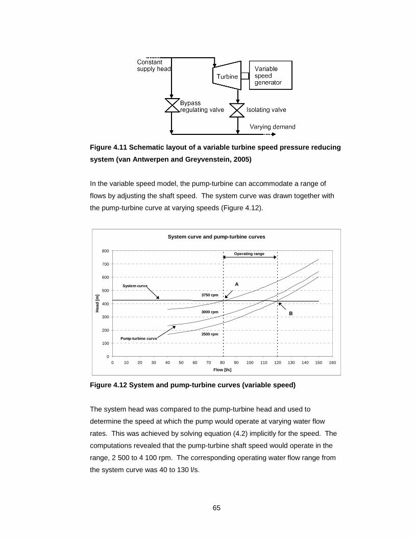
65
Figure 4.11 Schematic layout of a variable turbine speed pressure reducing
system (van Antwerpen and Greyvenstein, 2005)
In the variable speed model, the pump-turbine can accommodate a range of
flows by adjusting the shaft speed. The system curve was drawn together with
the pump-turbine curve at varying speeds (Figure 4.12).
System curve and pump-turbine curves
0
100
200
300
400
500
600
700
800
0 10 20 30 40 50 60 70 80 90 100 110 120 130 140 150 160
Flow [l/s]
Hea
d [m
] 3750 rpm
3000 rpm
2500 rpm
System curve
Pump-turbine curve
Operating range
Figure 4.12 System and pump-turbine curves (variabl e speed)
The system head was compared to the pump-turbine head and used to
determine the speed at which the pump would operate at varying water flow
rates. This was achieved by solving equation (4.2) implicitly for the speed. The
computations revealed that the pump-turbine shaft speed would operate in the
range, 2 500 to 4 100 rpm. The corresponding operating water flow range from
the system curve was 40 to 130 l/s.
A
B

66
The pump-turbine efficiency placed a constraint on the range of operating water
flow and shaft speed. The efficiency was calculated using equation (4.3) at the
determined flow rate/speed pairs (Figure 4.13). This reduced the operating flow
range to between 52 and 120 l/s.
A further constraint on the water flow range was the pump-turbine runaway speed
of 3 900 rpm11. The upper limit for the pump-turbine shaft speed was therefore
selected at 5 % below the runaway speed, namely, 3 750 rpm. Consequently,
the pump-turbine would operate between 2 500 and 3 750 rpm. The
corresponding water flow range was 80.7 to 120 l/s.
It should be noted that an increase in water flow through the pump-turbine results
in a decrease in the operating speed. This observation is consistent with the
variable speed pump-turbine model proposed by van Antwerpen and
Greyvenstein (2005). When the flow is 80.7 l/s the operating speed will be
3 750 rpm (point A, Figure 4.12). At point B, the operating speed has deceased
to 2 500 rpm and the flow has increased to 120 l/s.
Pump-turbine efficiency
0.0
0.1
0.2
0.3
0.4
0.5
0.6
0.7
0.8
0.9
0 10 20 30 40 50 60 70 80 90 100 110 120 130 140 150 160
Flow [l/s]
Effi
cien
cy
Figure 4.13 Pump-turbine efficiency curve (variable speed)
11 The pump-turbine manufacturer stated that the runaway speed for this pump-turbine
would be 130 % of the normal operating speed of 3 000 rpm (Tasker, 2011).

67
It has been shown that the (system) average water flow varies between 11.1 and
120.5 l/s. The pump-turbine operating range (80.7 to 120 l/s), could not
adequately cope with the system water flow range. This necessitated a bypass
line in parallel with the pump-turbine system to cater for water flows outside
pump-turbine flow range. Two pressure-reducing valves would be installed in
series in the bypass line to reduce the pressure from 52 bar to 10.5 bar.
This defined three modes of operation for the system (Table 4.7).
Table 4.7 Modes of operation for the pump-turbine s ystem at variable speed
Mode I Mode II Mode III
Water flow range 0 – 80.7 l/s 80.7 – 120 l/s > 120 l/s
System
configuration
Turbine off
Bypass open
Turbine on
Bypass closed
Turbine on
Bypass open
At low water flows (Mode I), the turbine would not operate, but pressure reduction
is achieved using the pressure-reducing valves. Mode II describes the turbine
operation, where energy will be recovered. The bypass also caters for higher
flow demands (Mode III), when the water flow increases above 120 l/s.
Depending on the mode of operation (Table 4.7), the overall efficiency will be
determined by the operation of the pressure-reducing valves and the pump-
turbine. When operating in Mode I, all the water will flow through the bypass and
the system efficiency will be zero (no energy will be recovered). When the flow
increases above 80.7 l/s, the system will then operate in Mode II and energy will
be recovered by the pump-turbine. The system efficiency will be the same as the
pump-turbine efficiency and determined using the regressed equation for the
efficiency [equation (4.3)].
When the system operates in Mode III, energy will be recovered by the pump-
turbine and energy will be dissipated across the pressure-reducing valves in the
bypass. The following relation can be used to determine the system efficiency,
ηSYS
ηSYS = η (q / qSYS) (4.4)

68
The maximum water flow through the pump-turbine q is 120 l/s and the
corresponding efficiency η is 80 %. The total flow entering the system will is qSYS.
The second alternative for the pump-turbine system is operation at constant shaft
speed. In Figure 4.11, the variable speed generator becomes a constant speed
generator; while the isolating valve becomes a pressure regulating valve (pp 65).
A shaft speed of 3 000 rpm (50 Hz) was selected since this corresponds to the
frequency of electrical power supplied by Eskom. This mitigated the need for
complex power electronics when connecting the system to the electrical power
grid (Section 4.3.5).
System curve and pump-turbine curves
0
100
200
300
400
500
600
700
800
0 10 20 30 40 50 60 70 80 90 100 110 120 130 140 150 160
Flow [l/s]
Hea
d [m
]
System curve
Pump-turbine curve3000 rpm
Figure 4.14 System and pump-turbine curves (constan t speed)
The operating water flow range for the pump-turbine system is 40 to 110 l/s
(Figure 4.15). A minimum flow of 40 l/s is required to prevent cavitation in the
pump-turbine. The upper limit for the flow range (110 l/s) was determined by the
intersection of the pump-turbine and system head curves. The pump-turbine can
not operate above 110 l/s since the system head is lower than the required
pump-turbine head.
∆Pvalve

69
An efficiency of 77.2 % is observed at the maximum water flow of 110 l/s.
However, the system efficiency below 110 l/s, was lower due to the presence of
the pressure-reducing valve in series.
A pressure-reducing valve is required in series with the pump-turbine since at
water flows below the operating point; the pump-turbine does not use the full
system head.
Pump-turbine efficiency
0.0
0.1
0.2
0.3
0.4
0.5
0.6
0.7
0.8
0.9
0 10 20 30 40 50 60 70 80 90 100 110 120 130 140 150 160
Flow [l/s]
Effi
cien
cy
Figure 4.15 Pump-turbine efficiency curve (constant speed)
Three modes of operation for the system were also defined for the constant
speed alternative (Table 4.8). A bypass line will also be installed to cater for
water flows outside the pump-turbine operating range. The bypass pressure
reducing valves would be the same as for the variable speed alternative.
The pump-turbine curve and system curve intersected at 110 l/s and defined the
upper limit for Mode II operation. The minimum flow was 40 l/s (Figure 4.15).

70
Table 4.8 Modes of operation for the pump-turbine s ystem at constant
speed
Mode I Mode II Mode III
Water flow range 0 – 40 l/s 40 – 110 l/s > 110 l/s
System
configuration
Turbine off
Bypass open
Turbine on
Bypass closed
Turbine on
Bypass open
The system efficiency is influenced by the pump-turbine and pressure-reducing
valves. In Mode I, no energy will be recovered and the efficiency will be zero.
When in Mode II, the system efficiency will depend on the pump-turbine efficiency
and energy dissipated by the valve installed in series. The relationship used was
ηSYS = η (h / hSYS) (4.5)
In the above equation, the system efficiency ηSYS was determined using the
pump-turbine efficiency η and head h at corresponding water flows.
Equation (4.3) was used when the system operated in Mode II only.
When the flow increased above 110 l/s, the bypass allowed additional water flow.
The system efficiency for Mode III of operation, involved the solution of
equation (4.5).
The system efficiency for variable and constant speed alternatives is shown
graphically below.

71
System efficiency
0.0
0.1
0.2
0.3
0.4
0.5
0.6
0.7
0.8
0.9
0 10 20 30 40 50 60 70 80 90 100 110 120 130 140 150 160
Flow [l/s]
Effi
cien
cy
Figure 4.16 System efficiency for variable and cons tant speed alternatives
The constant speed system would recover energy over a wider water flow range.
The variable speed system shows a steeper rise to peak efficiency with higher
efficiencies observed above 120 l/s. The constant speed system had a maximum
efficiency of 77.2 % at 110 l/s, while the variable speed system had a peak
efficiency of 80 % at 120 l/s.
Constant speed
system
Variable speed
system

72
Figure 4.17 Process flow diagram (FN-PT-10-001)
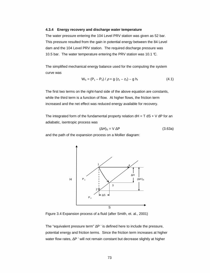
73
4.3.4 Energy recovery and discharge water temperatu re
The water pressure entering the 104 Level PRV station was given as 52 bar.
This pressure resulted from the gain in potential energy between the 84 Level
dam and the 104 Level PRV station. The required discharge pressure was
10.5 bar. The water temperature entering the PRV station was 10.1 °C.
The simplified mechanical energy balance used for the computing the system
curve was
WS = (P1 – P2) / ρ + g (z1 – z2) – g hf (4.1)
The first two terms on the right-hand side of the above equation are constants,
while the third term is a function of flow. At higher flows, the friction term
increased and the net effect was reduced energy available for recovery.
The integrated form of the fundamental property relation dH = T dS + V dP for an
adiabatic, isentropic process was
(∆H)S = V ∆P (3.63a)
and the path of the expansion process on a Mollier diagram:
H
S
P 1
P 2
∆H
(∆H )S
1
2
3
4
∆S
Figure 3.4 Expansion process of a fluid (after Smith, et. al., 2001)
The “equivalent pressure term” ∆P ' is defined here to include the pressure,
potential energy and friction terms. Since the friction term increases at higher
water flow rates, ∆P ' will not remain constant but decrease slightly at higher

74
water flows (the friction term is negative). The form was the same as defined
previously as
(∆H ')S = V ∆P ' (3.64)
and
(WS) S = (∆H ')S (3.65)
The value of ∆P ' used in the above equation was the value previously calculated
for generating the system curve. This value was 4 127 kPa at the design water
flow of 109.4 l/s. The enthalpy difference, at constant entropy, was 4.13 kJ/kg
while the maximum shaft power was 452 kW at the design condition.
The pump-turbine efficiency was given by the pump manufacturer (APPENDIX
C). After computing the isentropic enthalpy difference (∆H ')S, the actual enthalpy
difference across the turbine ∆H ' was calculated using
η = ∆H ' / (∆H ')S (3.66a)
The enthalpy difference ∆H ', was 3.19 kJ/kg and the hydraulic power was
349 kW at a predicted efficiency of 77.3 %.
The discharge water temperatures were then calculated using the Joule-
Thomson coefficients at constant entropy µS and constant enthalpy µH. The
temperature entering the turbine was 10.1 °C and is entropic process, path 1-2,
resulted in the water temperature reducing to 10.08 °C. However, the
temperature increased to 11.09 °C when the isenthal pic process, path 1-4, was
followed.
The water discharge temperature when the pump-turbine was present resulted in
a temperature greater that the isentropic process temperature and less than the
isenthalpic process temperature. This temperature was 10.32 °C.
4.3.5 Electrical design
The hydraulic power produced by a turbine system will be converted to electrical
power using an electrical drive. An induction machine was selected since it is
easy to maintain and common in industry. This eliminated the commutator-brush
system of the dc machine which is subject to mechanical breakdown.

75
For the variable speed alternative, the model predicted a hydraulic power
generated at the peak flow of 120 l/s (Mode II operation) of 394 kW at a pump-
turbine efficiency of 79.7 %. A 15 % safety margin was added to yield an
expected generated power of 454 kW. Therefore, a standard WEG induction
generator at a rated power of 500 kW was selected.
Figure 4.18 General arrangement of pump-turbine & g enerator – variable
speed (FN-PT-10-004)
The pump-turbine at constant speed is expected to generate 353 kW of power at
the peak flow of 110 l/s and efficiency of 77.3 % (maximum water flow for Mode II
operation). When the safety margin of 15 % was added, the power generated will
be 406 kW. Therefore, a WEG induction generator rated at 400 kW was
selected.

76
Figure 4.19 General arrangement of pump-turbine & g enerator – constant
speed (FN-PT-10-005)
It should be noted that the electrical losses within the induction generator were
assumed at 96 %12.
The power generated by the pump-turbine will be fed back into the electrical
power grid at a substation in the vicinity of the pump-turbine system. The stand-
alone system was not preferred since a local source that could utilise the power
was not available (i.e. a pump or fan).
The constant speed system will generate power at a shaft speed of 3 000 rpm or
50 Hz. This corresponded to the Eskom supply frequency and will therefore be
connected using an electrical cable (240 mm2, 4 core, low voltage, PVC
insulated) and WEG 400 kW switchgear. The switchgear would be installed in a
spare panel within the substation and cables would be routed from the electrical
drive to the substation. A loss factor of 5 %13 was assumed between the pump-
turbine system and the electrical system.
12 This value was taken from the datasheet provided by the manufacturer (APPENDIX C). 13 Eskom loss factors for transmission (0-300 km) and distribution (≥ 500 V and < 66 kV)
are 1.0096 and 1.0758 respectively. The average of these values is 1.043.

77
Figure 4.20 Single line diagram – variable speed (F N-PT-10-006)
The variable speed system will operate between 2 500 rpm and 3 750 rpm (42 to
63 Hz). This system will therefore require a WEG 500 kW variable frequency
drive (VFD) in addition to cabling (300 mm2, 4 core, low voltage, PVC insulated)
and a WEG VFD panel. The variable frequency drive panel will convert the
incoming variable frequencies to the supply frequency of 50 Hz.
Figure 4.21 Single line diagram – constant speed (F N-PT-10-007)
The power expected to be fed back into the grid by the variable speed alternative,
for the typical week is shown in Figure 4.22. At the average maximum water flow
of 109.4 l/s, the electrical power generated will be 318.5 kW. Since the lower
limit for the operating range in Mode II was 52 l/s, no energy is expected to be
recovered at a flow of 40.3 l/s.

78
Power profile (variable speed)
0
50
100
150
200
250
300
350
0:00 7:30 19:30 0:00 19:30 21:30 0:00 19:00 21:30 0:00 19:00 21:30 0:00 19:00 21:30 0:00 18:00 0:00
0:00 0:00 7:30 19:30 0:00 19:30 21:30 0:00 19:00 21:30 0:00 19:00 21:30 0:00 19:00 21:30 0:00 18:00
Sat Sunday Monday Tuesday Wednesday Thursday Friday
Ele
ctric
al p
ower
[kW
]
Figure 4.22 Power profile for a typical week (varia ble speed alternative)
For the constant speed alternative (Figure 4.23), the power generated at the
water flow of 109.4 l/s will be marginally higher at 319.1 kW; and at a flow of
40.3 l/s, 5.7 kW is expected to be recovered and fed back to the power grid.
Power profile (constant speed)
0
50
100
150
200
250
300
350
0:00 7:30 19:30 0:00 19:30 21:30 0:00 19:00 21:30 0:00 19:00 21:30 0:00 19:00 21:30 0:00 18:00 0:00
0:00 0:00 7:30 19:30 0:00 19:30 21:30 0:00 19:00 21:30 0:00 19:00 21:30 0:00 19:00 21:30 0:00 18:00
Sat Sunday Monday Tuesday Wednesday Thursday Friday
Ele
ctric
al p
ower
[kW
]
Figure 4.23 Power profile for a typical week (const ant speed alternative)

79
4.3.6 System operation and control
The pump-turbine system consists of various components to enable generation of
power and minimise the temperature increase of the water. Three modes of
operation have been defined in Section 4.3.3. Mode II describes the water flow
range in which the pump-turbine will operate. The bypass line with the pressure-
reducing valve is necessary for Mode I operation (low flow condition) and
Mode III operation (high flow condition). An Allen-Bradley programmable logic
controller (PLC) will be installed to monitor the system operation and provide
feedback on status of the system (normal, fault, failure). Tag numbers for valves
and instrumentation are indicated in the piping and instrumentation diagram
(Figure 4.24).

80
Figure 4.24 Piping and instrumentation diagram – va riable speed (FN-PT-10-
002)
A magnetic flow meter FE-101 will measure the water flow entering the system.
Two motorised control valves (FCV-101 and FCV-102) will be installed

81
downstream of the flow meter. When FCV-101 is open, water will flow to the
pump and when FCV-102 is open, water will flow through the bypass line.
Isolating manual valves (B25 and B20) are installed for maintenance purposes.
Pressure indicators (PI-101 and PI-102) are installed to measure the inlet and
outlet water pressures. Temperature indicators (TI-101 and TI-102) are installed
to measure the inlet and outlet water temperatures. In the event of a power
failure, FCV-101 will fail closed and FCV-102 will fail open.
In variable speed mode the pump-turbine will operate at varying shaft speeds,
ranging from 2 500 to 3 750 rpm (42 to 63 Hz). When the water flow is below
80.7 l/s, valve FCV-102 must open to allow the water to flow through the bypass
line. FCV-102 must remain closed (Mode I operation).
When the water flow exceeds 80.7 l/s, a signal must be sent to valve FCV-102 to
close and a signal must be sent to FCV-101 to open. This will allow the water to
flow through the pump-turbine. No water will flow through the bypass line
(Mode II operation).
When the water flow increases above 120 l/s, a signal will be sent to FCV-102 to
open while FCV-101 will remain open. This will allow the additional water above
120 l/s to flow through the bypass line (Mode III operation); while the maximum
water flow of 120 l/s will flow through the pump-turbine (FCV-101 will be open
and the pump speed will be 2 500 rpm).
A speed transmitter ST-101 will measure the pump-turbine shaft speed. When
the water flow is at 80.7 l/s, the pump-turbine will operate at a shaft speed of
3 750 rpm. When the water flow increases, the pump speed will reduce. The
maximum water flow through the pump system will be 120 l/s and the
corresponding pump speed will be 2 500 rpm. The speed of the pump-turbine
will adjust according to the system curve (Figure 4.12). In the event of the pump-
turbine shaft speed reaching the runaway speed of 3 900 rpm, valve FCV-101
must close and FCV-102 must open to allow the water to flow through the bypass
line.

82
In constant speed alternative (Figure 4.25), the pump will operate at a fixed
speed of 3 000 rpm (50 Hz). When the water flow is below 40 l/s, valve FCV-102
must open to allow the water to flow through the bypass line. FCV-101 must
remain closed (Mode I operation).
Figure 4.25 Piping and instrumentation diagram – co nstant speed (FN-PT-
10-003)
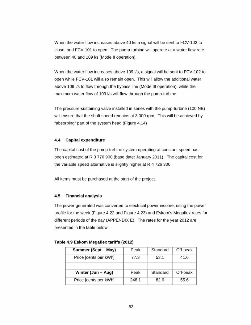
83
When the water flow increases above 40 l/s a signal will be sent to FCV-102 to
close, and FCV-101 to open. The pump-turbine will operate at a water flow rate
between 40 and 109 l/s (Mode II operation).
When the water flow increases above 109 l/s, a signal will be sent to FCV-102 to
open while FCV-101 will also remain open. This will allow the additional water
above 109 l/s to flow through the bypass line (Mode III operation); while the
maximum water flow of 109 l/s will flow through the pump-turbine.
The pressure-sustaining valve installed in series with the pump-turbine (100 NB)
will ensure that the shaft speed remains at 3 000 rpm. This will be achieved by
“absorbing” part of the system head (Figure 4.14)
4.4 Capital expenditure
The capital cost of the pump-turbine system operating at constant speed has
been estimated at R 3 776 900 (base date: January 2011). The capital cost for
the variable speed alternative is slightly higher at R 4 726 300.
All items must be purchased at the start of the project.
4.5 Financial analysis
The power generated was converted to electrical power income, using the power
profile for the week (Figure 4.22 and Figure 4.23) and Eskom’s Megaflex rates for
different periods of the day (APPENDIX E). The rates for the year 2012 are
presented in the table below.
Table 4.9 Eskom Megaflex tariffs (2012)
Summer (Sept – May) Peak Standard Off-peak
Price [cents per kWh] 77.3 53.1 41.6
Winter (Jun – Aug) Peak Standard Off-peak
Price [cents per kWh] 248.1 82.6 55.6

84
It should be noted that the periods during which power was generated by the
pump-turbine system did not correspond entirely within the Eskom tariff periods.
It was therefore necessary to allocate the power generated during the week into
the Eskom defined rate periods to obtain an acceptable estimate of the power
income. As an example, Figure 4.26 illustrates the power generated by the
constant speed alternative on the Friday, with the corresponding Eskom tariffs for
the summer months (low demand season).
Power profile for Friday (constant speed)
0
50
100
150
200
250
300
350
0:0
0
1:0
0
2:0
0
3:0
0
4:0
0
5:0
0
6:0
0
7:0
0
8:0
0
9:0
0
10
:00
11
:00
12
:00
13
:00
14
:00
15
:00
16
:00
17
:00
18
:00
19
:00
20
:00
21
:00
22
:00
23
:00
Ele
ctric
al p
ower
[kW
]
0
10
20
30
40
50
60
Esk
om ta
riff [
cent
s pe
r kW
h]
Eskom tariff
319.1 kW
5.7 kW
Figure 4.26 Power generated and Eskom tariffs for a Friday at constant
speed
For the typical week, the variable speed alternative generated 6 146 kWh during
the peak periods, 14 814 kWh during standard periods and 13 395 kWh during
off-peak periods. The electrical power income generated for the summer and
winter months for a week, are presented in Table 4.10.

85
Table 4.10 Electrical power income for a week in 20 12
Summer (Sept – May) Peak Standard Off-peak Total
Electrical power income [R] 4 801 7 952 5 635 18 388
Winter (Jun – Aug) Peak Standard Off-peak Total
Electrical power income [R] 15 407 12 370 7 521 35 298
It should be noted that the electrical power income listed in the above table would
be for the year 2011. Annual increases to these tariffs have been approved by
the National Energy Regulator of South Africa (NERSA). These tariffs will
increase by 25.8 % in 2011 and increase by a further 25.9 % in 2012. Years
2013 and 2014 will have 25 % increases in cost (Eskom, 2010). This has the
implication of higher electrical power income being generated in later years
(APPENDIX G).
A business case has been compiled for the pump-turbine system. Predicted
cash-flows for each year have been calculated using the above Eskom proposed
tariffs and presented in APPENDIX G. The projected cash flows over a ten-year
horizon are presented in Figure 4.27.
Projected cash flow
-6
-4
-2
0
2
4
6
8
10
2011 2012 2013 2014 2015 2016 2017 2018 2019 2020 2021
Cas
h in
flow
s (o
utflo
ws)
[R x
10
6 ]
5%
10%
15%
Figure 4.27 Projected cash inflows and outflows for the pump-turbine
system (variable speed)

86
Eskom have also stated that the tariff will increase annually by 6 % from 2016
(Eskom, 2010). However, the proposed increase can change in the interim. A
sensitivity analysis was therefore carried out for tariff increases of 5, 10 and
15 %. The cash inflow and outflows for the constant speed alternative is
presented below.
Projected cash flow
-6
-4
-2
0
2
4
6
8
10
2011 2012 2013 2014 2015 2016 2017 2018 2019 2020 2021
Cas
h in
flow
s (o
utflo
ws)
[R x
10
6 ]
5%
10%
15%
Figure 4.28 Projected cash inflows and outflows for the pump-turbine
system (constant speed)
4.5.1 Net present value and internal rate of return
The feasibility of the project was ascertained using the Net present value (NPV)
method. This economic model considers the time-value of money by
“discounting” the future cash flows to present day. The cash-flows are
discounted to present day by using the formula
NPV = (future cash-flows) x ( 1 + discount rate ) –n (4.6)
A discount rate of 10 % was used and over a ten year period (n), the NPV for the
pump-turbine system was R 11 564 500 for the variable speed alternative. The
NPV for the constant speed alternative was slightly higher at R 11 644 600.
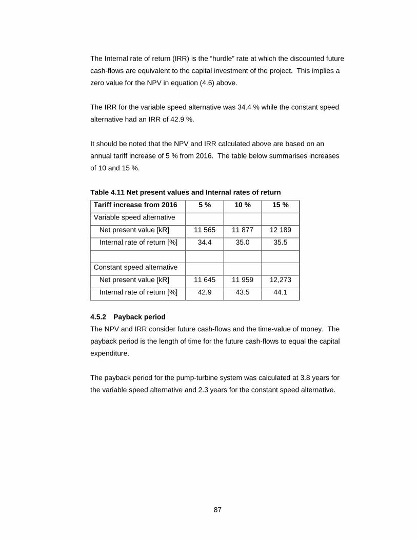
87
The Internal rate of return (IRR) is the “hurdle” rate at which the discounted future
cash-flows are equivalent to the capital investment of the project. This implies a
zero value for the NPV in equation (4.6) above.
The IRR for the variable speed alternative was 34.4 % while the constant speed
alternative had an IRR of 42.9 %.
It should be noted that the NPV and IRR calculated above are based on an
annual tariff increase of 5 % from 2016. The table below summarises increases
of 10 and 15 %.
Table 4.11 Net present values and Internal rates of return
Tariff increase from 2016 5 % 10 % 15 %
Variable speed alternative
Net present value [kR] 11 565 11 877 12 189
Internal rate of return [%] 34.4 35.0 35.5
Constant speed alternative
Net present value [kR] 11 645 11 959 12,273
Internal rate of return [%] 42.9 43.5 44.1
4.5.2 Payback period
The NPV and IRR consider future cash-flows and the time-value of money. The
payback period is the length of time for the future cash-flows to equal the capital
expenditure.
The payback period for the pump-turbine system was calculated at 3.8 years for
the variable speed alternative and 2.3 years for the constant speed alternative.

88
4.6 Project management
The project will take approximately 38 weeks to from project kick-off to
commissioning and hand-over. This includes all civil, mechanical and electrical
works. The items with the longest lead times are the pump-turbine set and VSD
and switchgear (16 and 22 weeks respectively). The project schedule is included
in APPENDIX H.
4.7 Conclusion
The data for the pressure reducing valve station on 104 Level was regressed to
obtain a design water flow and pressure. A suitable pump was thereafter
selected. Design criteria were defined and models proposed in the literature
were employed to predict the performance of the pump-turbine system. The
technical and economic feasibility of two alternative systems were subsequently
examined. The constant speed alternative was shown to be the better option. A
schedule was also provided for construction of the system.

89
5 CONCLUSION AND RECOMMENDATIONS
5.1 Summary of the project
A study has been carried out to ascertain the feasibility of replacing a pressure-
reducing valve with a turbine. This was achieved by using data received from
Anglogold Ashanti Mponeng mine. The data included water flows and pressure
data recorded at a pressure-reducing station located on 104 Level. A statistical
analysis and data regression was carried out and a typical operating week was
obtained. The average water flow through the station was 109.4 l/s with a
corresponding discharge pressure of 10.5 bar.
A multi-stage pump was selected at the design water flow and pressure. The
pump would operate in reverse i.e. the high pressure water will enter the pump
via the “discharge” nozzle and exit via the “suction” nozzle. Turbine curves for
the pump were provided by Sulzer and the pump selected was HPH 28-1S. The
pump-turbine curves for the head and efficiency was regressed using models
proposed by van Antwerpen and Greyvenstein (2005). The regressed models
were used to define two alternative systems; namely a variable shaft speed
system and a constant shaft speed system.
An operating water flow range was defined for each alternative system. The
quantity of energy expected to be recovered was calculated and would be fed
back to the electrical power grid. At the design water flow, the variable speed
system potentially generated 318.5 kW; while 319.1 kW would be generated at
constant speed. The discharge water temperature for both systems would be
10.32 °C.
Capital costs were compiled from budget quotations received from potential
suppliers and historical costs14. The variable speed system requires R 4 726 300
capital investment while the constant speed system costs R 3 776 900.
14 BBE Cost Database, 2010.

90
A financial analysis for the variable speed system revealed an NPV of
R 11 565 000; IRR of 34.4 % and payback of 3.8 years. The constant speed
system has an NPV of R 11 645 000; IRR of 42.9 % and payback of 2.3 years.
Both systems are technically and economically feasible. However, the constant
speed system would be the better alternative.
5.2 Recommendations for further work
It is recommended to progress beyond the current project scope into a
construction and testing phase.
The work would include the verification of the design calculations and predicted
results by experimental data. This can be achieved by procurement and
construction of the constant speed system and equipping the experimental site
with suitable data-logging systems.
The pump system will be installed in parallel to the existing pressure-reducing
station located on 104 Level. This is to ensure continuity of the chilled water
supply in the event that the experimental facility becomes unavailable due to any
number of factors.
5.3 Closure
The objective of the project was to evaluate the economic feasibility of replacing
a pressure reducing valve with a pressure reducing turbine. Towards that end,
an energy recovery system was designed using a standard pump that would
operate in reverse. It has been shown that the system would recover energy in a
manner that is both technically and economically feasible.

91
REFERENCES
ABERDARE POWER CABLES, (2009) “Cable facts and figures handbook”,
Aberdare Cables (Pty) Ltd, Gauteng.
ANONYMOUS, (Oct 2010), Eskom – Looking ahead (chief executive breakfast
presentation), Eskom, South Africa, Internet: http://www.eskom.co.za/tariffs.php,
27 Nov 2010.
ANONYMOUS, Selected historical exchange rates and other interest rates, South
African Reserve Bank, Internet:
http://www.resbank.co.za/Research/Rates/Pages/Rates-Home.aspx,
4 April 2011.
ARRIAGA M., (2010), Pump as turbine – A pico-hydro alternative in Lao People’s
Democratic Republic, Renewable Energy, Vol.35, pp 1109-1115.
BLUHM, S.J., HEMP, R., FUNNELL, R., SHEER, T.J., BUTTERWORTH, M.D.,
RAWLINS, A., (Apr 2000), Deepmine Task 6.5.3, Efficiency of chilled water
distribution systems, Bluhm Burton Engineering, Johannesburg, South Africa.
BLUHM, S.J., VON GLEHN, F.H., SMIT, H., (Feb 2003), Important basics of mine
ventilation and cooling planning, Journal of the Mine Ventilation Society of South
Africa, Conference Proceedings, CSIR Pretoria.
BUSE, F., (1981), Using centrifugal pumps as hydraulic turbines, Chemical
Engineering, pp 113-117.
CONRADIE, D., (Apr 2010), Tariffs and charges 2010/2011,
Internet: http://www.eskom.co.za/live/content.php, 27 Nov 2010.
CREAMER, M., (Jun 25, 2010), South Deep will prove to be one the best
investments ever made – Gold Fields, Mining Weekly, Creamer Media,
Johannesburg.

92
DERAKHSHAN, S., NOURBAKHSH, A., (2008), Theoretical, numerical and
experimental investigation of centrifugal pumps in reverse operation,
Experimental Thermal and Fluid Science, Vol. 32, pp 1620-1627.
DOUGLAS, J.F., GASIOREK, J.M., SWAFFIELD, J.A., (1995), Fluid Mechanics,
Third edition, Longman Group Limited, England.
DU TOIT, L., (2009), Mponeng simplified CW reticulation system, Anglogold
Ashanti Mponeng, North-west province, South Africa.
DU TOIT, L., (2010), Mponeng dam temperatures, Anglogold Ashanti Mponeng,
North-west province, South Africa.
FERGUSON, D.W.B., BLUHM, S.J., (Nov 1984), Performance testing of an
energy recovery turbine at a three-stage spray chamber, Journal of the Mine
Ventilation Society of South Africa, Vol. 37, pp 121-125.
FUNNELL, R.C., GUNDERSEN, R.E., BLUHM, S.J., VON GLEHN, F.H., (March
2006), The synergistic benefits and limitations of hydro-mine power for mine
cooling, South African Institute of Mining and Metallurgy Conference,
Johannesburg.
GEANKOPLIS, C.J., (1993), Transport Processes and Unit Operations, Third
Edition, Prentice-Hall, New Jersey.
GOPAL, A.K., HARPER, G.S., (Mar 1999), Deepmine Task 13.4.1, “Energy
recovery device, CSIR Miningtek, Johannesburg, South Africa.
GOPALAKRISHNAN, S., (1986), Power recovery turbines for the process
industry, Proceedings of the Third Pump Users Symposium, pp 3-11.
GRAY, C.B., (1989), Electrical Machines and Drive Systems, Longman Scientific
and Technical, England.

93
HOFFMAN, D., (Jul 1994), The installation of a 3-Chamber pipe-feeder system –
its effect on the design of the water reticulation system, Journal of the Mine
Ventilation Society of South Africa, Vol. 47, pp 142-144.
LAUX, C.H., (1982), Reverse-running standard pumps as energy recovery
turbines, Sulzer Technical Review, Vol. 2, pp 23-27.
LUYBEN, W.L., (1989), Process modelling, Simulation, and Control for Chemical
Engineers, Second Edition, McGraw-Hill, New York
MANKBADI R.R., MIKHAIL, S.A., (1984), A turbine-pump system for low-head
hydropower, Energy Conversion and Management, Vol.25, No. 3, pp 339-344.
MARAIS, J., (Feb 6, 2011), Oppenheimers reposition, Sunday Times,
Independent Newspapers, Gauteng, South Africa.
MASSEY, B.S., (1970) Mechanics of fluids, Second edition, Van Nostrand
Reinhold Company, Canada.
McPHERSON, M.J., (1993), Subsurface Ventilation and Environmental
Engineering, Chapman and Hall, London.
O’DONNELL, M.A., (Feb 19, 2010), The energy behind the world’s deepest gold
mine, Mining Weekly, Creamer Media, Johannesburg.
ORCHARD, B., KLOS, S., (2009), Pumps as turbines for water industry, World
Pumps, pp 22-23.
PATEL, M.R., (2006), Wind and Solar Power Systems, Second edition, CRC
Press, Florida.
PERRY, R.H., GREEN, D.W., (1997), Perry’s Chemical Engineers Handbook,
Seventh Edition, McGraw-Hill, New York.

94
PETERS, M.S., TIMMERHAUS, K.D., WEST, R.D., (2003), Plant Design and
economics for chemical engineers, Fifth Edition, McGraw-Hill, New York.
RAJA, W.A., PIAZZA, R.W., (1981), Reverse running centrifugal pumps as
hydraulic power recovery turbines for seawater reverse osmosis systems,
Desalination, Vol. 38, pp 123-134.
RAMOS, H., BORGA, A., (1999), Pumps as turbines: an unconventional solution
to energy production, Urban Water, Vol. 1, pp 261-263.
RAMSDEN, R., (Sept 1983), The temperature rise of chilled water flowing
through pipes, Journal of the Mine Ventilation Society of South Africa, Vol. 36,
pp 85-93.
RAMSDEN, R., BLUHM, S.J., (Sept 1985) Energy recovery turbines for use with
underground air coolers, Proceedings of the Second US Mine Ventilation
Symposium, Reno, Nevada, USA, pp 571-80.
RICHMOND, S.B., (1964) Statistical Analysis, Second edition, The Ronald Press
Company, New York
ROBBINS, A., (Mar 26, 2010), PRV Station data, Anglogold Ashanti Mponeng,
North-west province, South Africa.
SAYERS, A.T., (1946), “Hydraulic and Compressible Flow Turbomachines”,
Library of Congress Cataloging-in-Publication Data, Britain.
SCHOLL, H.G., (2000), A pump-turbine combination for sea water, World Pumps,
pp 24-25.
SMITH, J.M., Van Ness, H.C., Abbott, M.M., (2001), Introduction to Chemical
Engineering Thermodynamics, Sixth edition, McGraw-Hill, New York.
TASKER, M, (2011), Runaway speed, Sulzer, Gauteng, South Africa.

95
TORBIN, R.N., (1989), Alternate methods of energy recovery for the mining
industry, IEEE Transactions on Industry Applications, Vol. 25, No. 5, pp 811-818.
VAN ANTWERPEN, H.J., GREYVENSTEIN, G.P., (2005), Use of turbines for
simultaneous pressure regulation and recovery in secondary cooling water
systems in deep mines, Energy Conversion and Management, Vol. 46, pp 563-
575.
VAN DER MERWE, M.L., (Mar 1986), Power recovery from chilled water at the
Buffelsfontein gold mine Southern shaft, Journal of the Mine Ventilation Society
of South Africa, Vol. 39, pp 37-45.
WALTERS, D.M, PRETORIUS, A.R.W., (1994), How a three chamber pipe
feeder system operates, Journal of the Mine Ventilation Society of South Africa,
Vol. 47, pp 144-146.
WHILLIER, A., (Apr 1977), Recovery of energy from water going down mine
shafts, Journal of South African Institute of Mining and Metallurgy, Vol. 77
pp 183-186.
WILLIAMS, A.A., (1996) Pumps as turbines for low cost micro hydro power,
World Renewable Energy Congress, Denver, Colorado, USA, pp 1227-1234.

96
BIBLIOGRAPHY
ANONYMOUS, (1998), Pump-turbine research project completed, World Pumps,
pp 12.
CREAMER, M., (Apr 21, 2010), Gold Fields spotlights unrivalled riches of one-of-
a-kind South Deep gold mine, Mining Weekly, Creamer Media, Johannesburg.
CREAMER, M., (Feb 9, 2009), World’s new deepest mine ‘safe, cheap’ –
AngloGold, Mining Weekly, Creamer Media, Johannesburg.
FRASER, P., LE ROUX, D., (May 2008), Energy savings by recovering the
pressure head in mines: A review of the theoretical and practical issues
associated with the design, installation, operation and maintenance of the 3
Chamber pump systems (3CPS) and turbine energy recovery systems,
Proceedings of the Mine Ventilation Conference, CSIR Pretoria.
HEGERMAN, C., (Mar 1997), Optimising the cooling of the Vaal Reefs No.11
shaft underground environment and a description of refrigeration and energy
recover equipment used, Journal of the Mine Ventilation Society, Vol. 50, pp 18-
24.
KRAMERS, A.P., (Mar 2002), Deepmine Task 6.4.2: Assessment of three-pipe
chamber feeder (3CPF) technology, CSIR Miningtek, Johannesburg, South
Africa.
LAUX, C.H., (1980), Reversible multistage pumps as energy recovery turbines in
oil supply systems, Sulzer Technical Review, Vol. 2, pp 61-75.
MOHAN, N., UNDELAND, T.M., ROBBINS, W.P., (1995), Power Electronics:
Converters, Applications and Design, John Wiley and Sons, United States of
America.
NAUTIYAL, H., VARUN, KUMAR, A., (2010), Reverse running pumps analytical,
experimental and computational study: a review, Renewable and Sustainable
Energy Reviews, Vol. 14, pp 2059-2067.

97
O’DONNELL, M.A., (Jun 25, 2010), New-order mining rights approved for gold
mine expansion project, Mining Weekly, Creamer Media, Johannesburg.
SHAFER, L.L., (1982), Pumps as power turbines, Mechanical Engineering,
pp 40-43.
STEPANOFF, A.J., (1957), Centrifugal and Axial Flow Pumps, Second edition,
John Wiley and Sons, United States of America.
WILLIAMS, A.A., SMITH, N.P.A., BIRD, C., HOWARD, M., (1998), Pumps as
Turbines and Induction Motors as Generators for Energy Recovery in Water
Supply Systems, Journal of the Chartered Institution of Water and Environmental
Management, Vol. 12, pp 175-178.

98
APPENDIX A RAW DATA
A.1 104 Level PRV data
0
2
4
6
8
10
12
14
16
18
20
0:00 2:00 4:00 6:00 8:00 10:00 12:00 14:00 16:00 18:00 20:00 22:00 0:00
Time [hour]
Dis
char
ge p
ress
ure
[bar
]Friday, 19 March 2010
0
20
40
60
80
100
120
140
0:00 2:00 4:00 6:00 8:00 10:00 12:00 14:00 16:00 18:00 20:00 22:00 0:00
Time [hour]
Flo
w [l
/s]

99
plot day formula:
0
2
4
6
8
10
12
14
16
18
20
0:00 2:00 4:00 6:00 8:00 10:00 12:00 14:00 16:00 18:00 20:00 22:00 0:00
Time [hour]
Dis
char
ge p
ress
ure
[bar
]
Head
Saturday, 20 March 2010
0
20
40
60
80
100
120
140
0:00 2:00 4:00 6:00 8:00 10:00 12:00 14:00 16:00 18:00 20:00 22:00 0:00
Time [hour]
Flo
w [l
/s]

100
p1 + 2880 - 1 = p2
Sunday, 21 March 2010
0
20
40
60
80
100
120
140
0:00 2:00 4:00 6:00 8:00 10:00 12:00 14:00 16:00 18:00 20:00 22:00 0:00
Time [hour]
Flo
w [l
/s]
0
2
4
6
8
10
12
14
16
18
20
0:00 2:00 4:00 6:00 8:00 10:00 12:00 14:00 16:00 18:00 20:00 22:00 0:00
Time [hour]
Dis
char
ge p
ress
ure
[bar
]

101
Monday, 22 March 2010
0
20
40
60
80
100
120
140
0:00 2:00 4:00 6:00 8:00 10:00 12:00 14:00 16:00 18:00 20:00 22:00 0:00
Time [hour]
Flo
w [l
/s]
0
2
4
6
8
10
12
14
16
18
20
0:00 2:00 4:00 6:00 8:00 10:00 12:00 14:00 16:00 18:00 20:00 22:00 0:00
Time [hour]
Dis
char
ge p
ress
ure
[bar
]

102
0
2
4
6
8
10
12
14
16
18
20
0:00 2:00 4:00 6:00 8:00 10:00 12:00 14:00 16:00 18:00 20:00 22:00 0:00
Time [hour]
Dis
char
ge p
ress
ure
[bar
]
Tuesday, 23 March 2010
0
20
40
60
80
100
120
140
0:00 2:00 4:00 6:00 8:00 10:00 12:00 14:00 16:00 18:00 20:00 22:00 0:00
Time [hour]
Flo
w [l
/s]

103
0
2
4
6
8
10
12
14
16
18
20
0:00 2:00 4:00 6:00 8:00 10:00 12:00 14:00 16:00 18:00 20:00 22:00 0:00
Time [hour]
Dis
char
ge p
ress
ure
[bar
]
Wednesday, 24 March 2010
0
20
40
60
80
100
120
140
0:00 2:00 4:00 6:00 8:00 10:00 12:00 14:00 16:00 18:00 20:00 22:00 0:00
Time [hour]
Flo
w [l
/s]

104
Thursday, 25 March 2010
0
20
40
60
80
100
120
140
0:00 2:00 4:00 6:00 8:00 10:00 12:00 14:00 16:00 18:00 20:00 22:00 0:00
Time [hour]
Flo
w [l
/s]
0
2
4
6
8
10
12
14
16
18
20
0:00 2:00 4:00 6:00 8:00 10:00 12:00 14:00 16:00 18:00 20:00 22:00 0:00
Time [hour]
Dis
char
ge p
ress
ure
[bar
]

105
0
2
4
6
8
10
12
14
16
18
20
0:00 2:00 4:00 6:00 8:00 10:00 12:00 14:00 16:00 18:00 20:00 22:00 0:00
Time [hour]
Dis
char
ge p
ress
ure
[bar
]
Friday, 26 March 2010
0
20
40
60
80
100
120
140
0:00 2:00 4:00 6:00 8:00 10:00 12:00 14:00 16:00 18:00 20:00 22:00 0:00
Time [hour]
Flo
w [l
/s]

106
A.2 99 Level PRV data
Friday, 19 March 2010
0
5
10
15
20
25
30
35
40
0:00 2:00 4:00 6:00 8:00 10:00 12:00 14:00 16:00 18:00 20:00 22:00 0:00
Time [hour]
Flo
w [l
/s]
0
2
4
6
8
10
12
14
16
18
0:00 2:00 4:00 6:00 8:00 10:00 12:00 14:00 16:00 18:00 20:00 22:00 0:00
Time [hour]
Dis
char
ge p
ress
ure
[bar
]

107
Saturday, 20 March 2010
0
5
10
15
20
25
30
35
40
0:00 2:00 4:00 6:00 8:00 10:00 12:00 14:00 16:00 18:00 20:00 22:00 0:00
Time [hour]
Flo
w [l
/s]
0
2
4
6
8
10
12
14
16
18
0:00 2:00 4:00 6:00 8:00 10:00 12:00 14:00 16:00 18:00 20:00 22:00 0:00
Time [hour]
Dis
char
ge p
ress
ure
[bar
]

108
Sunday, 21 March 2010
0
5
10
15
20
25
30
35
40
0:00 2:00 4:00 6:00 8:00 10:00 12:00 14:00 16:00 18:00 20:00 22:00 0:00
Time [hour]
Flo
w [l
/s]
0
2
4
6
8
10
12
14
16
18
0:00 2:00 4:00 6:00 8:00 10:00 12:00 14:00 16:00 18:00 20:00 22:00 0:00
Time [hour]
Dis
char
ge p
ress
ure
[bar
]

109
Monday, 22 March 2010
0
5
10
15
20
25
30
35
40
0:00 2:00 4:00 6:00 8:00 10:00 12:00 14:00 16:00 18:00 20:00 22:00 0:00
Time [hour]
Flo
w [l
/s]
0
2
4
6
8
10
12
14
16
18
0:00 2:00 4:00 6:00 8:00 10:00 12:00 14:00 16:00 18:00 20:00 22:00 0:00
Time [hour]
Dis
char
ge p
ress
ure
[bar
]

110
0
2
4
6
8
10
12
14
16
18
0:00 2:00 4:00 6:00 8:00 10:00 12:00 14:00 16:00 18:00 20:00 22:00 0:00
Time [hour]
Dis
char
ge p
ress
ure
[bar
]
Tuesday, 23 March 2010
0
5
10
15
20
25
30
35
40
0:00 2:00 4:00 6:00 8:00 10:00 12:00 14:00 16:00 18:00 20:00 22:00 0:00
Time [hour]
Flo
w [l
/s]

111
0
2
4
6
8
10
12
14
16
18
0:00 2:00 4:00 6:00 8:00 10:00 12:00 14:00 16:00 18:00 20:00 22:00 0:00
Time [hour]
Dis
char
ge p
ress
ure
[bar
]
Wednesday, 24 March 2010
0
5
10
15
20
25
30
35
40
0:00 2:00 4:00 6:00 8:00 10:00 12:00 14:00 16:00 18:00 20:00 22:00 0:00
Time [hour]
Flo
w [l
/s]

112
Thursday, 25 March 2010
0
5
10
15
20
25
30
35
40
0:00 2:00 4:00 6:00 8:00 10:00 12:00 14:00 16:00 18:00 20:00 22:00 0:00
Time [hour]
Flo
w [l
/s]
0
2
4
6
8
10
12
14
16
18
0:00 2:00 4:00 6:00 8:00 10:00 12:00 14:00 16:00 18:00 20:00 22:00 0:00
Time [hour]
Dis
char
ge p
ress
ure
[bar
]

113
Friday, 26 March 2010
0
5
10
15
20
25
30
35
40
0:00 2:00 4:00 6:00 8:00 10:00 12:00 14:00 16:00 18:00 20:00 22:00 0:00
Time [hour]
Flo
w [l
/s]
0
2
4
6
8
10
12
14
16
18
0:00 2:00 4:00 6:00 8:00 10:00 12:00 14:00 16:00 18:00 20:00 22:00 0:00
Time [hour]
Dis
char
ge p
ress
ure
[bar
]

114
APPENDIX B REGRESSION OF WATER FLOW DATA
The purpose of regressing the data is to identify a weekly trend. This was
achieved using descriptive statistics. Statistical theory will be presented below,
followed by calculations and a justification of the values selected.
B.1 Statistical analysis 15
The average value (¯ ) of a data range, is the sum of the observations in the data
range divided by the number of observations (n) in the range. Mathematically,
(¯ ) = ∑ x / n (B.1)
The average value in isolation is of little significance. The standard deviation (s)
gives an indication of how wide the data varies from the average; and is
calculated using
s = [ ∑ (x – ¯ )2 / (n – 1) ] ½ (B.2)
In a data range, the median divides the data such that half of the observations
and larger and half are smaller. The mode of the range is the value in the data
range with highest number of occurrences.
The above parameters provide information on the tendency of data to centre
about a particular value. As an example, when the median and mode of the data
range are equal, the data is symmetrical about that value.
B.2 104 Level station data
The water flow through the 104 Level pressure-reducing valve station shows
three distinct ranges; and the flows have been classified as peak, intermediate
and low. A histogram of the raw data shows these ranges below.
15 Richmond, S.B., 1964
x
x
x

115
Water flow histogram
0
200
400
600
800
1000
1200
1400
1600
1800
2000
9 15 20 25 30 35 41 46 51 56 61 67 72 77 82 87 93 98 103 108 113 119 124 129 134
Water flow [l/s]
Fre
quen
cy
Low flow range
Intermediate flow range
High flow range
15.5 l/s
40.7 l/s
109.1 l/s
Figure B1 Histogram for water flow through the 104 Level station
The value indicated in each flow range (Figure B1) is the mode. Table B1 lists
the statistical parameters that were calculated from the data for the week.
Table B1 Statistical analysis of water flow data
Water flow [l/s] Low Intermediate Peak
Sample size (n) 4 491 5 267 12 197
Average (¯ ) 15.6 40.3 109.4
Standard deviation (s) 3.1 1.1 7.7
Median 15.3 40.3 108.8
Mode 15.5 40.7 109.1
The average value was used in the calculations since central tendency about this
value is observed (a marginal difference is noted between the average, median
and mode).
x

116
APPENDIX C MANUFACTURER’S DATA
C.1 Pump-turbine curves (Sulzer)

117
C.2 Induction generator performance curves (Zest en ergy)
Figure C1 500 kW induction generator for variable s peed alternative
Figure C2 400 kW induction generator for constant s peed alternative

118
APPENDIX D SAMPLE CALCULATIONS
D.1 System Curve
The system curve (Figure 3.6, pp 40) was generated determining the available
shaft work, at a range of water flows. A flow of 110 l/s and discharge pressure of
10.5 bar will be used to illustrate the methodology.
The system under consideration is
The mechanical energy balance has been derived as
(P1 – P2) / ρ + g (z1 – z2) – g hf = WS (4.1)
and multiplying the equation by density ρ gives
(P1 – P2) + ρ g (z1 – z2) – ρ g hf = ρ WS
The available work WS = 4 150 + 4.41 – 27.8 = 4 127 kPa
• Pressure term: P1 – P2 = (52 – 10.5) bar x 100 kPa / bar = 4 150 kPa
• Potential energy term: ρ g (z1 – z2) = 1 000 x 9.79 x 0.45 = 4 406 Pa = 4.41 kPa
ρ = 1 000 kg/m3 g = 9.79 m/s2
z1 – z2 = 0.45 m (elevation difference between suction and
discharge centre-lines)
• Friction loss term: ρ g hf = sum of friction losses (pipe, pipe fittings and
valves)
= 3 x (0.597) + 5.76 + 3.11 + 6.76 + 5.28 + 1.76
= 25.2 kPa
A design factor of 10 % was added to the total friction loss to give 27.8 kPa
PUMP-TURBINE
52 bar
250 mm
109.4 l/s
10.5 bar
250 mm

119
From the P&ID (FN-PT-10-002) the following fittings are present:
Loss coefficient Pressure loss
Butterfly valves (3-off) KL = 0.24 KL ρ u2 / 2
Anti-vibration joint (1-off) KL = 0.3 KL ρ u2 / 2
Anti-vibration joint (1-off) KL = 0.3 KL ρ u2 / 2
Reducer (1-off) KL = 0.55(1 – A2/A1) KL ρ u22 / 2
Diffuser (1-off) KL =(1 – A1/A2) KL ρ u12 / 2
For a butterfly valve, KL ρ u2 / 2 = 0.24 x 1 000 x 2.232 / 2 = 597 Pa = 0.597 kPa
D = 250 mm A = π / 4 x D2 = π / 4 x 0.252 = 0.049 m2
u = q / A = 109.4 / 0.049 / 1 000 = 2.23 m/s
Similarly, the pressure losses for the anti-vibration joints are 5.76 kPa
(150 mm) and 3.11 kPa (175 mm).
For the reducer, KL ρ u22 / 2 = 0.55 (1 – A2/A1) ρ u2
2 / 2 = 0.55(1 –
0.018/0.049) 1 000 x 6.202 / 2
= 6758 Pa =
6.76 kPa
D1 = 250 mm A = π / 4 x D2 = π / 4 x 0.252 = 0.049 m2
D2 = 150 mm A = π / 4 x D2 = π / 4 x 0.152 = 0.018 m2
u = q / A = 109.4 / 0.018 / 1 000
= 6.20 m/s
(velocity at the smaller area is used)
Similarly, the pressure loss for the diffuser is 5.28 kPa.
The pipe friction was 4f (L / D) ρ u2 / 2
= 4 x 0.0037 x (12 / 0.25) 1 000 x 2.232 / 2
= 1757 Pa
= 1.76 kPa

120
The friction factor was solved implicitly using the Colebrook equation
1 / f½ = – 4 log [ε / 3.7 D + 1.256 / (Re f½)]
= – 4 log [0.07 / 3.7 (0.25) + 1.256 / (4.16 x 10⁸ f½)]
Therefore, f = 0.0037
ε = 0.07 mm (1.5 times the roughness of a new steel pipe –
0.046 mm)
Re = Lu ρ / µF
= 0.25 x 2.23 x 1 000 /
1.34 x 10-6
= 4.16 x 10⁸
(characteristic length L will be the
pipe diameter D)
D.2 Pump-turbine curves
The pump-turbine curve provided by the manufacturer was regressed to give
(Section 4.3.2)
h = s (6.50 x 10⁻³ q2 – 1.01 x 10⁻⁴ q N + 6.67 x 10⁻⁶ N2)
For the variable speed alternative, the speed N was solved implicitly, at a given
water flow q and corresponding system head h. At the design flow of 109.4 l/s,
the system head was 421.8 m. Substituting into the above equation (s = 4
stages) yields
421.8 = 4 { 6.50 x 10⁻³ (109.4)2 – 1.01 x 10⁻⁴ (109.4) N + 6.67 x 10⁻⁶ N2 }
Hence, N = 3014 rpm
At constant speed, N = 3 000 rpm. Both water flow and speed are known, and
are inserted on the right-hand side in the above equation. At 109.4 l/s
H = 4 { 6.50 x 10⁻³ (109.4)2 – 1.01 x 10⁻⁴ (109.4) (3 000) + 6.67 x 10⁻⁶ (3 000)2 }
And H = 420.1 m. The pressure drop across the valve would be the difference
between the system and pump-turbine head.

121
D.3 System Efficiency
The pump-turbine efficiency curve provided by the manufacturer was regressed
to give (Section 4.3.2)
η = 1.55 x 10⁵ φ4 – 9.21 x 10³ φ3 – 1.00 x 10³ φ2 + 88.5 φ – 0.949
where φ is the flow to speed ratio, q/N. At the design flow, φ = 109.4 / 3 014 =
0.036 l/s per rpm. Therefore, the pump-turbine efficiency is
η = 1.55 x 10⁵ (0.036)4 – 9.21 x 10³ (0.036)3 – 1.00 x 10³ (0.036)2 + 88.5 (0.036)
– 0.949
and η = 0.773 or 77.3 %.
The system efficiency is defined by the mode of operation. In Mode I, the water
flows through the bypass and no energy is recovered, therefore the system
efficiency is zero. In Mode II, the system efficiency would be equivalent to the
pump-turbine efficiency when operating at variable speed. At water flows above
the flow at which peak efficiency is observed, the system efficiency reduces
according to
ηSYS = η (q / qSYS) (4.4)
At a water flow of 130 l/s,
ηSYS = 0.797 (120 / 130)
and ηSYS = 0.736 or 73.6 %.
At constant speed (3 000 rpm), the series pressure-reducing valve will reduce the
system efficiency when the pump-turbine operates (Mode II) according to
ηSYS = η (h / hSYS) (4.5)
The peak flow for Mode II was 110 l/s and the efficiency was 77.2 %. At a flow of
90 l/s,
ηSYS = 0.772 (342.5 / 422.7)
therefore ηSYS = 0.553 or 55.3 %.

122
At a flow above 110 l/s (Mode III operation), equation (4.5) is used,
ηSYS = 0.772 (110 / 130)
and ηSYS = 0.652 or 65.2 %.
D.4 Energy recovered
The energy recovered by the pump-turbine was calculated. A flow of 109.4 l/s
and discharge pressure of 10.5 bar will be used to illustrate the methodology.
∆P ' = 4 127 kPa (equivalent pressure term from system curve
calculation)
For the variable speed alternative,
Enthalpy difference (isentropic) Maximum shaft power
(∆H ')S = V ∆P '
= 0.001 x 4127
= 4.127 kJ/kg
(WS)S = q (∆H ')S
= 109.4 x 4.127
= 451 kW
Enthalpy difference (actual) Actual pump-turbine power
∆H ' = η (∆H ')S
= 0.773 x 4.127
= 3.19 kJ/kg
WS = η (WS)S
= 0.773 x 452
= 349 kW
The pump-turbine efficiency is used above to calculate the energy recovered (not
system efficiency ηSYS).
D.5 Energy fed into the power grid
The energy recovered by the pump-turbine at a flow of 109.4 l/s was 349 kW for
the variable speed alternative. The generator efficiency was assumed at 96 %
and the electrical system loss was 5 %.
Power at electrical drive = 0.96 x 349 kW
= 335 kW

123
Power fed into grid = (1 – 0.05) x 335 kW
= 319 kW
When the system operation changes from Mode II to Mode III, the water entering
the system will flow through the bypass, while the pump-turbine still operates.
Therefore, in Mode III energy will be generated and fed into the grid.
D.6 Discharge water temperatures
The pump-turbine outlet water temperature was calculated. A flow of 109.4 l/s
and discharge pressure of 10.5 bar will be used to illustrate the methodology.
• Isenthalpic discharge water temperature: using the Joule-Thomson coefficient
at constant enthalpy ,
µH = (∂T / ∂P)H ≈ ∆T / ∆P ' = (T1 – T4) / ∆P '
Rearranging results in
T4 = T1 – µH ∆P '
= 10.1 – (-0.2388) x 4.127
= 11.09 °C
• Isentropic discharge water temperature: using the Joule-Thomson coefficient
at constant entropy,
µS = (∂T / ∂P)S ≈ ∆T / ∆P ' = (T1 – T2) / ∆P '
Rearranging results in
T2 = T1 – µS ∆P '
= 10.1 – (0.006) x 4.127
= 10.08 °C
• Actual pump-turbine discharge water temperature: the enthalpy change
across the pump-turbine,
∆H ' = CP (T4 – T3)
and ∆H ' = ηSYS (∆H ')S
= ηSYS V ∆P '

124
Rearranging results in
T3 = T4 – ηS V ∆P ' / CP
= 10.1 – 0.773 (0.001) 4.127 / 4.194
= 10.32 °C
The system efficiency was used to calculate discharge temperature since it
considers the presence of the series pressure reducing valve (constant speed
alternative) and bypass pressure reducing valve (both alternatives).
D.7 Electrical cable sizing
The cables that were selected for the pump-turbine system was based on a
calculation outlined in a handbook published by Aberdare Cables.
The full-load current IFL was calculated using the following relation:
IFL = P * 1000 / (3½ * V * cos φ)
where, P is the power in kW, V is the supply voltage and cos φ is the power factor
(0.9).
Therefore, for the variable speed alternative,
IFL = 394 * 1000 / (3½ * 525 * 0.9) = 482 Amps
From Table 6.2, pp 38, the current rating close to the above full load amps is
509 Amps for a cable size of 300 mm2. This cable can carry 509 Amps
continuously when installed under standard conditions in air.
The voltage drop is calculated using the voltage drop factor (0.189 mV/A/m, from
Table 6.2) and the starting current. Since the pump-turbine will be direct on line,
the full load amps are multiplied by a factor of 6. A distance of 25 m was
assumed between the induction generator and the substation.
Hence
Volt drop = 0.189 mV/A/m x 6 x 482 x 25 m / 1000 = 13.7 volts
The percentage voltage drop was 13.7 / 525 x 100 = 2.6 %

125
The 300 mm2, 4 core, SWA low voltage cable selected is acceptable (the
maximum voltage drop allowed by SABS 0142-1978 is 5 %).
Similarly for the constant speed alternative, the cable selected was 240 mm2,
4 core, SWA low voltage (the percentage voltage drop calculated was 2.6 %).
D.8 Electrical power income
The financial analysis involves in the calculation of the electrical power income.
This will be illustrated below for the variable speed alternative.
Eskom has defined time periods during the week that have different tariff
charges, namely, peak, standard and off-peak (Table D2). The calculation of the
final values is illustrated in APPENDIX E.
Table D2: Eskom Megaflex tariffs (2012)
Summer (Sept – May) Peak Standard Off-peak
Price [cents per kWh] 77.3 53.1 41.6
Winter (Jun – Aug) Peak Standard Off-peak
Price [cents per kWh] 248.1 82.6 55.6
Depending on the period during which power is generated, the power income
would be different.

126
Table D3 Power generated during Eskom defined perio ds
318.5 kW 0 kW 0 kW
Hours Peak Standard Off-peak Peak Std Off-peak
Mon 4.5 9.5 8.0 – – – 2.0
Tues 4.0 9.5 8.0 – – – 2.5
Wed 4.0 9.5 8.0 – – – 2.5
Thurs 4.0 9.5 8.0 – – 2.5
Fri 3.0 9.0 6.0 2.0 2.0 2.0 –
Sat – – – – 7.0 17 –
Sunday – – 4.5 – – 7.5 12
Multiplication of the power with the operating hours gives kilowatt-hours (Table
D4).
Table D4 Energy generated during Eskom defined peri ods
kWh Peak Standard Off-peak
Monday 1 433 3 026 2 548
Tuesday 1 274 3 026 2 548
Wednesday 1 274 3 026 2 548
Thursday 1 274 3 026 2 548
Friday 956 2 867 1 911
Saturday 0 0 0
Sunday 0 0 1 433
Total 6 211 14 970 13 536
Finally, the electrical power income is determined by multiplying the respective
Megaflex cost (Table D2) by the energy generated. The income is listed in the
table below.

127
Table D5 Electrical power income for a week (2012)
Summer (Sept – May) Peak Standard Off-peak Total
Electrical power income [R] 4 801 7 952 5 635 18 388
Winter (Jun – Aug) Peak Standard Off-peak Total
Electrical power income [R] 15 407 12 370 7 521 35 298
D.9 Present value calculation
The compound interest concept was used to “convert” the costs listed in the
Literature review to an equivalent present day value (2011). The formula used
was (Peters, et. al., 2003)
FV = PV (1 + i)n
where FV is the future amount, that includes the present amount or principle
(PV), i is the interest rate based on length of one interest period; while n is the
number of time units or interest periods. The energy saving of R 70 500 in 1977,
will be “converted” to an equivalent value in 2011.
Annual interest rates were obtained from published data (by the South African
Reserve Bank) from 1977 and 2011. Average annual interest rates were used.
(When a change in the rate occurred during the year, the average rate was
obtained by summing the interest rates scaled by the fraction of months the rate
prevailed out of 12 months).
The average interest rate i, calculated from 1977 to 2011, is 15.4 %, while the
number of interest periods is 34 years. Substituting in the above equation yields
FV = 70 500 (1 + 0.154)34
FV = 9 232 500
The other costs have also been “converted” present day value by adopting this
approach. Table D6 summarises the values.

128
Table D6 Summary of present value costs
Year PV [R] i [%] n [years] FV [R]
1977 70 500 15.4 34 9 232 500
1977 60 15.4 34 7 900
1984 200 15.9 27 11 300
1986 45 000 15.5 25 1 717 300
1989 99 770 15.6 22 2 534 500
1996 6 440 14.4 15 50 100
2000 2 000 000 12.6 11 7 610 200
The costs shown for 1989 and 1996 were $ 38 000 and $ 1 500 respectively.
These values were converted to Rand using the average annual exchange rate.
The average rand-dollar exchange rate in 1989 was R 2.60 per $; while in 1996,
the average exchange rate was R 4.30 per $ (from data published by the South
African Reserve Bank).

129
APPENDIX E ESKOM TARIFFS
Eskom publishes the tariff charges to its urban, residential and rural customers.
A year is split into a high demand season and a low demand season. The winter
months, June to August would fall under the high demand season and have
higher tariffs. The remainder of the year (September to May) would be classified
as low demand season having lower tariff charges.
The seasons are further divided into three regions, namely peak, standard and
off-peak. These define different charges for weekdays and weekends; as well as
different times of the day. The regions are described in Figure E1 below.
Figure E1 Eskom’s defined time of use periods (Conr adie, 2010)
Furthermore, distance also influences the cost through a transmission network
charge. This depends on the distance from a central point in Johannesburg and
described in Figure E2. For a distance under 300 km, there is no additional
charge. Between 300 and 600 km a surcharge of 1% is added. A further 300 km
would increase the cost by a further percent. Where the radial distance exceeds
900 km, the transmission network charge would be increased by 3%.

130
Figure E2 Transmission zones and applicable percent ages (Conradie, 2010)
Mponeng is charged Megaflex rates and the calculation of the cost will be
illustrated below. The remaining charges are shown graphically for a weekday
and Saturday in Figure E3 and Figure E4 respectively. The off-peak rate would
apply for the entire of Sunday.
The Active energy charge during the high demand season and a peak period is
142.38 c/kWh. The transmission zone is less than 300 km and the voltage is
between 500 volts and 66 kilovolts. Adding the environmental levy of 2 c/kWh
gives 144.38 c/kWh.
A reactive energy charge of 5.89 c/kvarh is levied. This value is divided by the
power factor (0.96) to convert it to 6.14 c/kWh. It should be noted that during the
low demand season, there is no charge for reactive energy. A rate-rebalancing
levy of 3.09 c/kWh is also included.
Distribution network charges would include a network access charge
(R 6.72 per kVA/month); a network demand charge (R 12.73 per kVA/month) and
a transmission network charge (R 3.35 per kVA/month). The network demand
charge is the highest actual demand during peak and standard periods for given
month. Assuming the distribution network charges to be 25% higher than the
continuous rate, the total charge would be 4.12 c/kWh.

131
Capital charges would include a service charge (R 1 638.73 per account/day) and
an administration charge (R 52.33 per day). Assuming 25 MW of continuous
absorbed power, the total charge would be 0.27 c/kWh.
Combining the above, the peak cost during the high demand season would be
158 c/kWh.
0102030405060708090
100110120130140150160170180190200
0:00
1:00
2:00
3:00
4:00
5:00
6:00
7:00
8:00
9:00
10:0
0
11:0
0
12:0
0
13:0
0
14:0
0
15:0
0
16:0
0
17:0
0
18:0
0
19:0
0
20:0
0
21:0
0
22:0
0
23:0
0
0:00
Ene
rgy
cost
[c p
er k
W h
our]
NOMINAL ELECTRICAL POWER COST [MEGAFLEX 2010]
WINTER
SUMMER26.533.8
49.2
35.4
52.6
158.0
Weekday
Figure E3 Nominal Megaflex tariff for a weekday
0
10
20
30
40
50
60
70
80
0:00
1:00
2:00
3:00
4:00
5:00
6:00
7:00
8:00
9:00
10:0
0
11:0
0
12:0
0
13:0
0
14:0
0
15:0
0
16:0
0
17:0
0
18:0
0
19:0
0
20:0
0
21:0
0
22:0
0
23:0
0
0:00
Ene
rgy
cost
[c p
er k
W h
our]
NOMINAL ELECTRICAL POWER COST [MEGAFLEX 2010]
WINTER
SUMMER26.5
33.8
35.4
52.6
Saturday
Figure E4 Nominal Megaflex tariff for a Saturday
The Eskom published rates are also included.

132
APPENDIX F CAPITAL EXPENDITURE
Base date: March 2011
ITEM DESCRIPTION NOTESConstant Variable
speed speed
1.0 Civil and Structural 4,200 4,7001.1 Pump-motor plinth 3,700 4,200 Note 11.2 Pipe supports 500 500 Note 2
2.0 Mechanicals 2,354,500 2,316,0002.1 Pump-turbine set 1,324,600 1,324,600 Note 32.2 Piping and pipe fittings 148,100 148,100 Note 42.3 Manual valves 278,300 278,300 Note 52.4 Control valves 320,000 320,000 Note 62.5 Pressure-reducing valves 283,500 245,000 Note 6
3.0 Electrical and instrumentation 662,800 1,460,3003.1 Switchgear 110,200 789,700 Notes 8, 93.2 Induction generator 260,800 399,800 Note 83.3 Programmable logic controller (PLC) 162,000 162,000 Note 103.4 Instrumentation (temperature, pressure, etc) 108,800 108,800 Note 73.5 Miscellaneous (cabling, etc) 21,000 25,000 Note 10
4.0 General 755,400 945,3004.1 Installation and commissioning [15% of direct costs] 453,200 567,200 Note 104.2 Contingencies [10% of direct costs] 302,200 378,100 Note 10
TOTAL 3,776,900 4,726,300
Notes[1]
[2][3][4][5][6][7][8][9][10]
Budget quotation from Zest Energy.
COST [R]
Clamp-type support assumed to be R100 each (estimate from BBE cost database).
Budget quotation from potential suppliers (Macsteel, CU Engineering).
Includes earthworks, concrete, formed and unformed surfaces and re-bar. Costs have been
estimated from drawings and sizes of equipment and an overall cost of R11,000 per m3 was used
Budget quotation from Sulzer (supply only).
Estimated from BBE cost database.
Budget quotation from potential suppliers (HPE, Macsteel).Budget quotation from HPE.Budget quotation from potential suppliers (Mecosa, Wika, IFM).
For the Variable speed alternative, the VSD cost is included with the Switchgear cost.
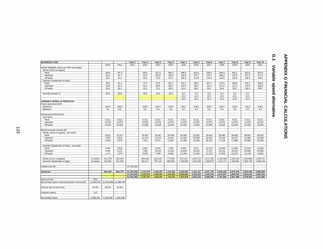
133
AP
PE
ND
IX G
FIN
AN
CIA
L CA
LCU
LAT
ION
S
G.1
Variable speed alternative
BUSINESS CASE Year 0 Year 1 Year 2 Year 3 Year 4 Year 5 Year 6 Year 7 Year 8 Year 9 Year 102010 2011 2011 2012 2013 2014 2015 2016 2017 2018 2019 2020 2021
Eskom Megaflex [cents per kWh (average)]Winter (June to August)
Peak 158.0 197.2 248.1 312.3 390.4 488.0 512.4 538.0 564.9 593.1 622.8 653.9Standard 52.6 65.7 82.6 104.0 130.0 162.6 170.7 179.2 188.2 197.6 207.5 217.8Off-peak 35.4 44.2 55.6 70.0 87.4 109.3 114.8 120.5 126.5 132.9 139.5 146.5
Summer (September to May)Peak 49.2 61.4 77.3 97.3 121.7 152.1 159.7 167.7 176.0 184.8 194.1 203.8Standard 33.8 42.2 53.1 66.9 83.6 104.5 109.7 115.2 121.0 127.0 133.4 140.0Off-peak 26.5 33.1 41.6 52.4 65.5 81.9 86.0 90.3 94.8 99.5 104.5 109.7
Annual increase % 24.8 25.8 25.9 25.0 25.0 5.0 5.0 5.0 5.0 5.0 5.010.0 10.0 10.0 10.0 10.0 10.015.0 15.0 15.0 15.0 15.0 15.0
VARIABLE SPEED ALTERNATIVEPower generated (kW)
Maximum 318.5 318.5 318.5 318.5 318.5 318.5 318.5 318.5 318.5 318.5 318.5 318.5Minimum 0.0 0.0 0.0 0.0 0.0 0.0 0.0 0.0 0.0 0.0 0.0 0.0
Energy generated (kWh)One week
Peak 6,211 6,211 6,211 6,211 6,211 6,211 6,211 6,211 6,211 6,211 6,211 6,211Standard 14,970 14,970 14,970 14,970 14,970 14,970 14,970 14,970 14,970 14,970 14,970 14,970Off-peak 13,536 13,536 13,536 13,536 13,536 13,536 13,536 13,536 13,536 13,536 13,536 13,536
Electrical power income (R)Winter (June to August) - one week
Peak 9,813 12,247 15,407 19,397 24,246 30,308 31,823 33,414 35,085 36,839 38,681 40,615Standard 7,879 9,833 12,370 15,573 19,467 24,333 25,550 26,828 28,169 29,577 31,056 32,609Off-peak 4,791 5,979 7,521 9,470 11,837 14,796 15,536 16,313 17,128 17,985 18,884 19,828
Summer (September to May) - one weekPeak 3,058 3,816 4,801 6,044 7,556 9,444 9,917 10,413 10,933 11,480 12,054 12,656Standard 5,065 6,321 7,952 10,012 12,515 15,644 16,426 17,247 18,110 19,015 19,966 20,964Off-peak 1,270 1,979 5,635 7,095 8,869 11,086 11,640 12,222 12,833 13,475 14,148 14,856
Winter (June to August) 14 weeks 314,759 392,819 494,166 622,156 777,694 972,118 1,020,724 1,071,760 1,125,348 1,181,616 1,240,696 1,302,731Summer (September to May) 34 weeks 319,381 411,956 625,211 787,141 983,926 1,229,908 1,291,403 1,355,974 1,423,772 1,494,961 1,569,709 1,648,194
Capital cost (R) (4,726,300)
Summary 634,140 804,775 (4,726,300) 1,119,378 1,409,297 1,761,621 2,202,026 2,312,127 2,427,734 2,549,120 2,676,576 2,810,405 2,950,926(4,726,300) 1,119,378 1,409,297 1,761,621 2,202,026 2,422,229 2,543,340 2,670,507 2,804,032 2,944,234 3,091,446(4,726,300) 1,119,378 1,409,297 1,761,621 2,202,026 2,532,330 2,658,946 2,791,894 2,931,489 3,078,063 3,231,966
Discount rate 10%Net present value of electrical power income (R) 11,564,542 11,876,669 12,188,796
Internal rate of return (%) 34.4% 35.0% 35.5%
Payback (years) 3.8
Net surplus (loss) 6,838,242 7,150,369 7,462,496

134
G.2
Constant speed alternative
BUSINESS CASE Year 0 Year 1 Year 2 Year 3 Year 4 Year 5 Year 6 Year 7 Year 8 Year 9 Year 102010 2011 2011 2012 2013 2014 2015 2016 2017 2018 2019 2020 2021
Eskom Megaflex [cents per kWh (average)]Winter (June to August)
Peak 158.0 197.2 248.1 312.3 390.4 488.0 512.4 538.0 564.9 593.1 622.8 653.9Standard 52.6 65.7 82.6 104.0 130.0 162.6 170.7 179.2 188.2 197.6 207.5 217.8Off-peak 35.4 44.2 55.6 70.0 87.4 109.3 114.8 120.5 126.5 132.9 139.5 146.5
Summer (September to May)Peak 49.2 61.4 77.3 97.3 121.7 152.1 159.7 167.7 176.0 184.8 194.1 203.8Standard 33.8 42.2 53.1 66.9 83.6 104.5 109.7 115.2 121.0 127.0 133.4 140.0Off-peak 26.5 33.1 41.6 52.4 65.5 81.9 86.0 90.3 94.8 99.5 104.5 109.7
Annual increase % 24.8 25.8 25.9 25.0 25.0 5.0 5.0 5.0 5.0 5.0 5.0 5.010.0 10.0 10.0 10.0 10.0 10.0 10.015.0 15.0 15.0 15.0 15.0 15.0 15.0
CONSTANT SPEED ALTERNATIVEPower generated (kW)
Maximum 319.1 319.1 319.1 319.1 319.1 319.1 319.1 319.1 319.1 319.1 319.1 319.1Minimum 5.7 5.7 5.7 5.7 5.7 5.7 5.7 5.7 5.7 5.7 5.7 5.7
Energy generated (kWh)One week
Peak 6,235 6,235 6,235 6,235 6,235 6,235 6,235 6,235 6,235 6,235 6,235 6,235Standard 15,051 15,051 15,051 15,051 15,051 15,051 15,051 15,051 15,051 15,051 15,051 15,051Off-peak 13,714 13,714 13,714 13,714 13,714 13,714 13,714 13,714 13,714 13,714 13,714 13,714
Electrical power income (R)Winter (June to August) - one week
Peak 9,851 12,294 15,466 19,471 24,339 30,424 31,945 33,542 35,219 36,980 38,829 40,771Standard 7,922 9,886 12,437 15,658 19,572 24,465 25,688 26,973 28,322 29,738 31,224 32,786Off-peak 4,854 6,057 7,620 9,594 11,992 14,990 15,740 16,527 17,353 18,220 19,132 20,088
Summer (September to May) - one weekPeak 3,070 3,831 4,819 6,068 7,585 9,481 9,955 10,452 10,975 11,524 12,100 12,705Standard 5,093 6,356 7,995 10,066 12,583 15,728 16,515 17,341 18,208 19,118 20,074 21,078Off-peak 1,287 2,005 5,709 7,188 8,985 11,231 11,792 12,382 13,001 13,651 14,334 15,051
Winter (June to August) 14 weeks 316,763 395,320 497,313 626,117 782,646 978,307 1,027,223 1,078,584 1,132,513 1,189,139 1,248,596 1,311,025Summer (September to May) 34 weeks 321,279 414,500 629,814 792,936 991,170 1,238,962 1,300,910 1,365,956 1,434,254 1,505,966 1,581,265 1,660,328
Capital cost (R) (3,776,900)
Summary 638,042 809,820 (3,776,900) 1,127,127 1,419,052 1,773,816 2,217,270 2,328,133 2,444,540 2,566,767 2,695,105 2,829,860 2,971,353(3,776,900) 1,127,127 1,419,052 1,773,816 2,217,270 2,438,996 2,560,946 2,688,994 2,823,443 2,964,615 3,112,846(3,776,900) 1,127,127 1,419,052 1,773,816 2,217,270 2,549,860 2,677,353 2,811,221 2,951,782 3,099,371 3,254,339
Discount rate 10%Net present value of electrical power income (R) 11,644,597 11,958,885 12,273,173
Internal rate of return (%) 42.9% 43.5% 44.1%
Payback (years) 2.3
Net surplus (loss) 7,867,697 8,181,985 8,496,273

135
APPENDIX H PROJECT SCHEDULE