Study on synchronization of coupled oscillators using the Fokker-Planck equation
37
synchronization of coupled oscillators using the Fokker-Planck equation H.Sakaguchi Kyushu University, Japan Fokker-Planck equation: important equation in statistical physics Synchronization in coupled oscillators
-
Upload
fitzgerald-walsh -
Category
Documents
-
view
36 -
download
4
description
Study on synchronization of coupled oscillators using the Fokker-Planck equation. H.Sakaguchi Kyushu University, Japan. Fokker-Planck equation: important equation in statistical physics Synchronization in coupled oscillators. Langevin equation. Stochastic differential equation - PowerPoint PPT Presentation
Transcript of Study on synchronization of coupled oscillators using the Fokker-Planck equation

Study on synchronization of coupled oscillators using the
Fokker-Planck equationH.Sakaguchi
Kyushu University, Japan
Fokker-Planck equation: important equation in statistical physics Synchronization in coupled oscillators

Langevin equation
Stochastic differential equation
Time evolution in a noisy environment
)()( txFdt
dx
Langevin equationX(t): a stochastic variable such as a position or a membrane potentialξ(t): a random force, Gaussian white noise

Random forcesGaussian:
The probability distribution function is Gaussian with average 0 and variance 2D.
White: There is no time correlation.
)'(2)'()( ttDtt Consider a large number of independent stochastic variables which obey the Langevin eq.
The stochastic variables are randomly distributed, since the random forces are different.

Fokker-Planck equation
Consider the probability density P(x,t) that the stochastic variable takes a value x.
P obeys the Fokker-Planck equation
2
2)(
x
PD
x
FP
t
P
Drift term Diffusion term
The probability density drifts with velocity F(x) and diffuses owing to the random force

Random walkNo drift force
t
dttxtxtdt
dx
xF
0 )()0()( ),(
,0)(
Langevin equation
Dt
xx
DtP
x
PD
t
P
4
))0((exp
4
1
,
2
2
2
Fokker-Planck equation

Ornstein-Ulenbeck process
Linear force ( v : velocity,- k v viscous force)
)(vv
v)v(
tkdt
d
kF
Fokker-Planck equation
Maxwell distribution
Stationary distribution
Brownian motion of a small particle such as a pollen on water surface
Tk
m
D
k
D
kP
PD
Pk
t
P
B2
vexp
2
vexp
2
,vv
)v(
22
2
2

Thermal equilibrium distribution
)(
)(
tx
U
dt
dxx
UxF
Potential force
Fokker-Planck equation
Tk
xUP
x
PD
x
xPU
t
P
B
)(exp
,)/(
2
2
D=kBT; T: Temperature
Thermal equilibrium distributionNo probability flow: Detailed balance

Fokker-Planck equation for coupled Langevin equations
Coupled Langevin equations for two variables
)'(2)'()( ),(),(
)'(2)'()( ),(),(
2222
1111
ttDtttyxGdt
dy
ttDtttyxFdt
dx
Fokker-Planck equation for P(x,y)
2
2
22
2
1
)),(()),((
y
PD
x
PD
y
PyxG
x
PyxF
t
P

Synchronization of coupled biological oscillators
Synchronization of flashing of fireflies.
Synchronization of cell activity in suprachiasmaticnucleus which control the circadian rhythms
Sleep spindle waves are brain waves which appear in the second stage of sleep. Spindle waves are created by synchronous firing
of inhibitory neurons in thalamus. (Steriade et al.)
Human EEG

Phase oscillatorsLimit cycle oscillation
Phase description:
phase variables
Two-coupled phase oscillators
K
KKdt
d
Kdt
d
Kdt
d
Kdt
d
2 for 0
,2 for )2() () (
)sin(2 )(
), sin(
), sin(
2 1
2 122
2 12 1
2 1 212 1
2 122
1211
Mutual Entrainment
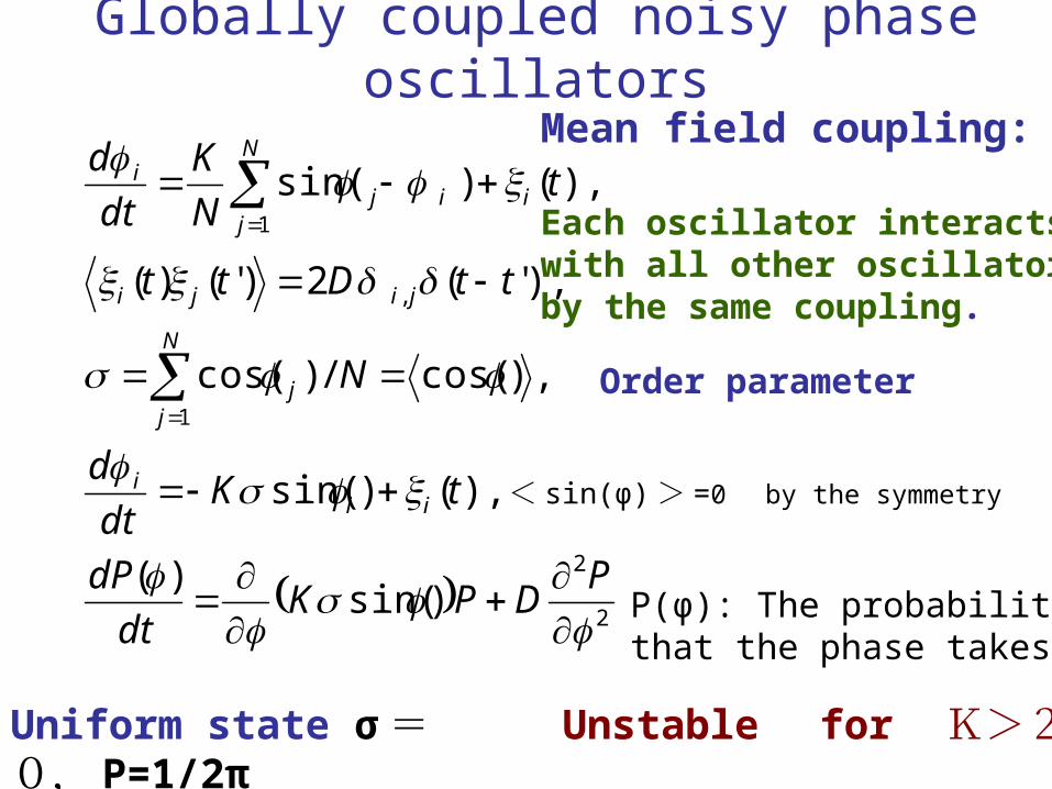
Globally coupled noisy phase oscillators
2
2
1
,
1
)sin()(
),()sin(
,)cos(/)cos(
),'( 2)'()(
),() sin(
PDPK
dt
dP
tKdt
d
N
ttDtt
tN
K
dt
d
iii
N
jj
jiji
i
N
jij
i
Uniform state σ =0, P=1/2πUnstable for K>2D
P(φ): The probability that the phase takes φ
Mean field coupling:
Each oscillator interactswith all other oscillatorsby the same coupling.
Order parameter
< sin(φ) > =0 by the symmetry

Self-Consistent MethodOrder parameter
12
16 ,
162
by expansionTaylor
)cos(
exp)(
)sin(
)cos()( )cos(
3
33
2
2
2
0
D
K
K
D
D
K
D
K
D
KP
PDPK
t
P
dP

Order-Disorder transitionWeak interaction, Large noise
Phases are randomly distributed.
Disordered phase.
Strong interaction, small noise
Phases gather together.
< cos(φ )> is nonzero.
Ordered state
Order-Disorder transition
Phase transition from ferromagnetism to paramagentism
If a magnet is heated above a critical temperature,
the magnetism disappears.

Globally coupled oscillators with different frequencies
rotation: , ||For
ent Entrainm)/(sin , ||For
sin
)cos(
)g(-)g( , of ondistributi :)g(
timeinconstant but random :
,) sin(
1
1
ii
iii
iii
N
jiji
i
K
KK
Kdt
d
N
K
dt
d
Phase oscillator model
Kuramoto model

Self-Consistent analysis
KK
Kdtd
gK
KKg
gK
gKKg
dg
c
c
c
||for )(
||for 0/
,|)0("|
))(0(8
)0(
2
,)0("16
)0(2
expansionTaylor
)())(cos(
22
3
33
ω

Globally coupled oscillators with different frequencies and external noises
2
2
,
1
)sin(),(
),() sin(
,)cos(
),'( 2)'()(
),() sin(
PDPK
dt
dP
tKdt
d
ttDtt
tN
K
dt
d
iiii
jiji
i
N
jiji
i
g(ω): Distribution of the natural frequency ω

Stationary solution of the Fokker-Planck equation for nonzero ω
2
0
0
))cos(1())cos(1(
2
2
)0()2( :ity Periodic,1)( :ionNormalizat
)0(),(
,0)sin(),(
PPdP
deD
cPeP
PDPK
t
P
D
K
D
K
Flow of probability: average circulation of phase Stationary but non-equilibrium distribution

Phase transition via synchronization
Complete entrainment is impossible owing to noises
22
2/1
22
2
0
2
1
,)(
)/()(
1
for unstable is state Uniform
)cos(),()(
)cos(
D
K
KK
DdDgKK
ddPg
c
c

Integrate-and-fire modelHodgkin-Huxley equation
Detailed dynamics of membrane potential
and several ion channels
IF model
simplest model of the neural firing
0. reset to is ,1 If
1for ,
xx
,xbxIdt
dx
x:membrane potential

Synchronization of two IF neurons
fires.neuron other when theby shifts variableThe
fires.neuron second) (thefirst when thejth time theis )(
,)(1
,)(1
21
122
211
gx
tt
ttgbxdt
dx
ttgbxdt
dx
jj
j
j
Instantaneous interactionResponse time 0
Complete synchronization for t>80
01.0 ,8.0 gb
δx=x1-x2
Noisy integrate-and-fire model and the Fokker-Planck equation
,10for ,
1)0(
,0for )0(
ondistributi Stationary
)/(
,)()(
xfor equationPlanck -Fokker
)'(2)'()( ),(
1
0
/}2/1 ({
0
/)}2/1 ({
/)2/1 (
/)2/1 (
10
02
2
2
2
2
2
xdze
dzeeP
xePP
xPDJ
Jxx
PDPbxI
xt
P
ttDtttbxIdt
dx
DbzzI
x DbzzI
DbxxI
DbxxI
x
reset process

Stochastic resonance in the noisy IF model
Stochastic resonanceResponse of excitable systems to periodic force + noises
Response is maximum for intermediate strength of noise
.0for 1:solution Stationary
system, Excitable
1 ),'(2)'()(
),()sin(1
,
eD/bx
bttDtt
ttebxdt
dx
jiji
iii

Direct simulation of the Fokker-Planck equation
ly.periodical changes )/( rate Firing
,)())sin(1(
equationPlanck -Fokker
10
02
2
xxPDJ
Jxx
PDPbxte
xt
P
Firing rateOscillation of P
Oscillation of J0
D=0.005,0.0015 b=1.1,e=0.05

Phase transition in a globally coupled IF models
)(
),()(}))(1{(
neuron kth theof timefiring jth : ,)(
)()(1
0
02
2
1
tgJIdt
dI
tJxx
PDPtIbx
xt
P
tttN
gI
dt
dI
ttIbxdt
dx
jk
N
k j
jk
iii
Oscillation amplitude vs. D
Disorder
Order
b=0.8,D=0.215,g=0.6,τ=0.01
τ : response time

Phase transition in a nonlocally coupled IF model
|)'|exp(48.0|)'|4exp(8.1)'(
,')'()'(),(
),,()()(
),,()(})),(1{(),(
0
02
2
yyyyyyg
dyyJyygtyJ
tyJyIdt
ydI
tyJxx
PDPytIbx
xt
yxP
Nonlocal interactionMaxican-hat type
Excitatory in the neighborhoodInhibitory in far regions
Synaptic coupling is nonlocal.Synaptic current at y is determined by the firing rate at y’ by the integral.
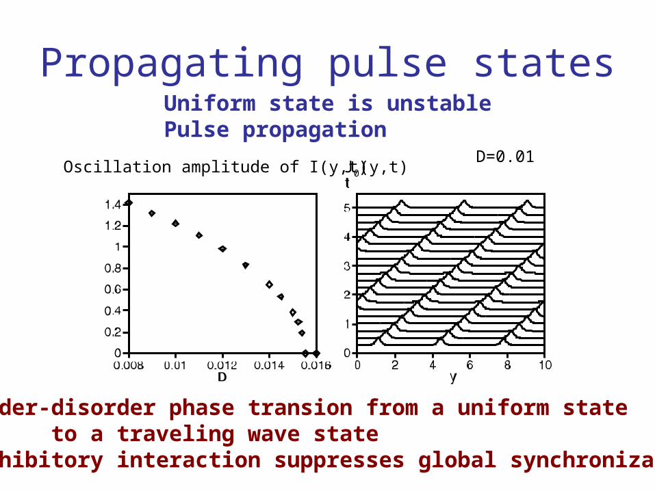
Propagating pulse statesUniform state is unstable Pulse propagation
Oscillation amplitude of I(y,t) J0(y,t)
Order-disorder phase transion from a uniform state to a traveling wave stateInhibitory interaction suppresses global synchronization
D=0.01

Another IF model and inhibitory networkThalamus(thalamic reticular neurons) Synchronization occurs among inhibitory neurons. Synchronization between two inhibitory IF neurons is possible if the response time τtakes a suitable value. Another IF model including the dynamics of excited state
50 ,35' ,30
40, -35, ,2,035.0
. tojumps , todown goes If
. tojumps ,over goes If
for )'(
for )(
200
2
22
1
0
0
VVV
VVC
VVVV
VVVV
VVVVdt
dVC
VVVVdt
dVC
TT
iTi
iTi
Tiii
Tiii
V>VT Excited state
VT
V1VT2
V2

Two IF neurons with inhibitory coupling
Synchronization of two inhibitory IF neurons
0for 0 ,0for 1)(
,)}(2/{
for ,)'(
for ,)(
2
1
0
0
VVV
VKIdt
dI
VVIVVdt
dVC
VVIVVdt
dVC
jjs
s
Tisii
Tisii
-Is inhibitory synapse
V1 and V2 are synchronized
K=0.5,V0=-18
Synchronization becomes easier owing to finite duration of excited state

Phase transition in globally coupled IF models with mutual inhibition
0
2211
2
2
0
1
0
)(
),()()()(
}),,({
,)(
)(),,(
dxxPKIdt
dI
tJVxtJVxx
PDPIIVf
xt
P
VN
KI
dt
dI
tIIVfdt
dV
i
N
jj
iii
Langevin equation
Fokker-Planck equation

Oscillatory phase transition in inhibitory systems
Oscillation amplitude vs. K
τ
Phase diagram
D=0.2,τ=20 D=0.2
Finite response time is preferable for global oscillation
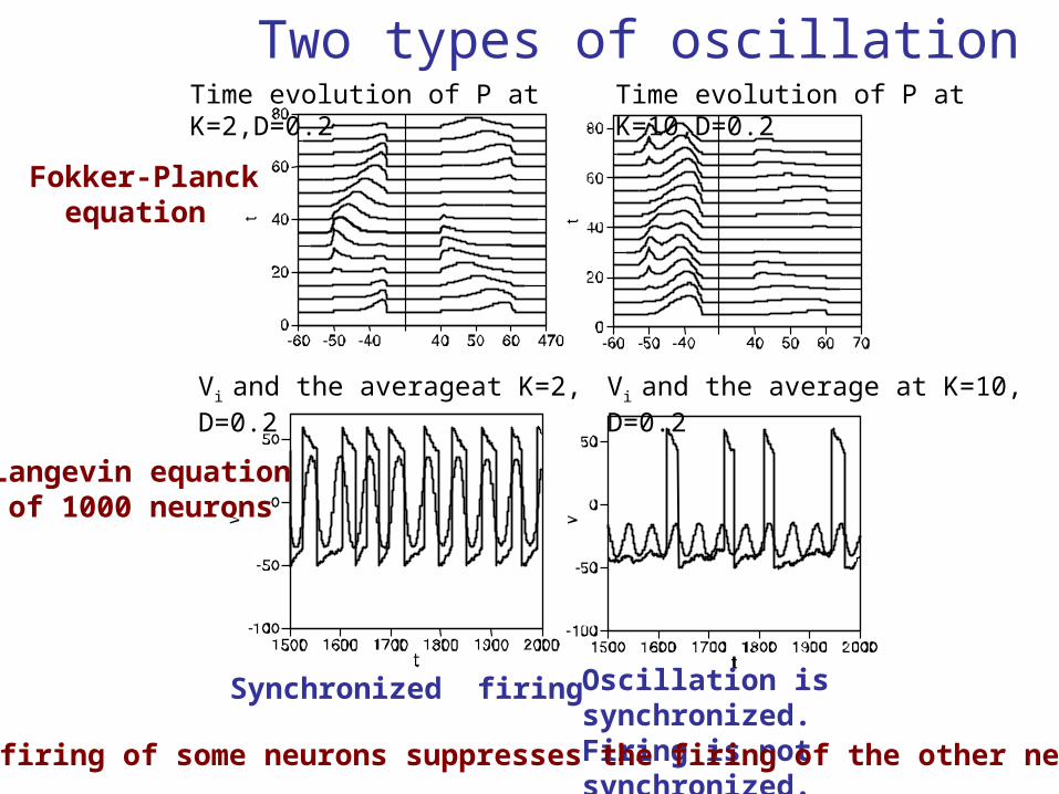
Vi and the average at K=10, D=0.2Vi and the averageat K=2, D=0.2
Time evolution of P at K=10,D=0.2Time evolution of P at K=2,D=0.2
Two types of oscillation
Oscillation is synchronized.Firing is not synchronized.
Fokker-Planck equation
Langevin equation of 1000 neurons
Synchronized firing
The firing of some neurons suppresses the firing of the other neurons
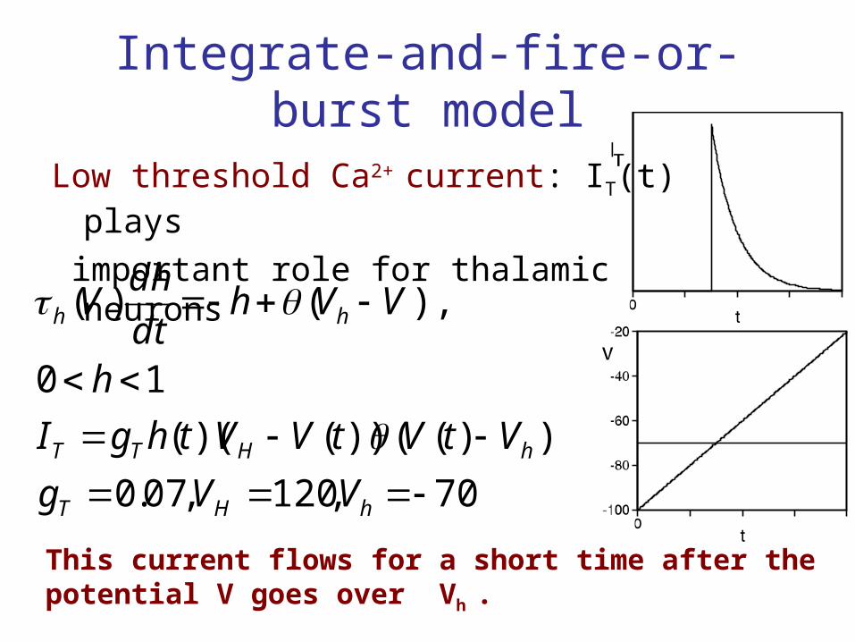
Integrate-and-fire-or-burst model
Low threshold Ca2+ current: IT(t) plays
important role for thalamic neurons
70,120,07.0
))(())()((
10
),()(
hHT
hHTT
hh
VVg
VtVtVVthgI
h
VVhdt
dhV
This current flows for a short time after the potential V goes over Vh .
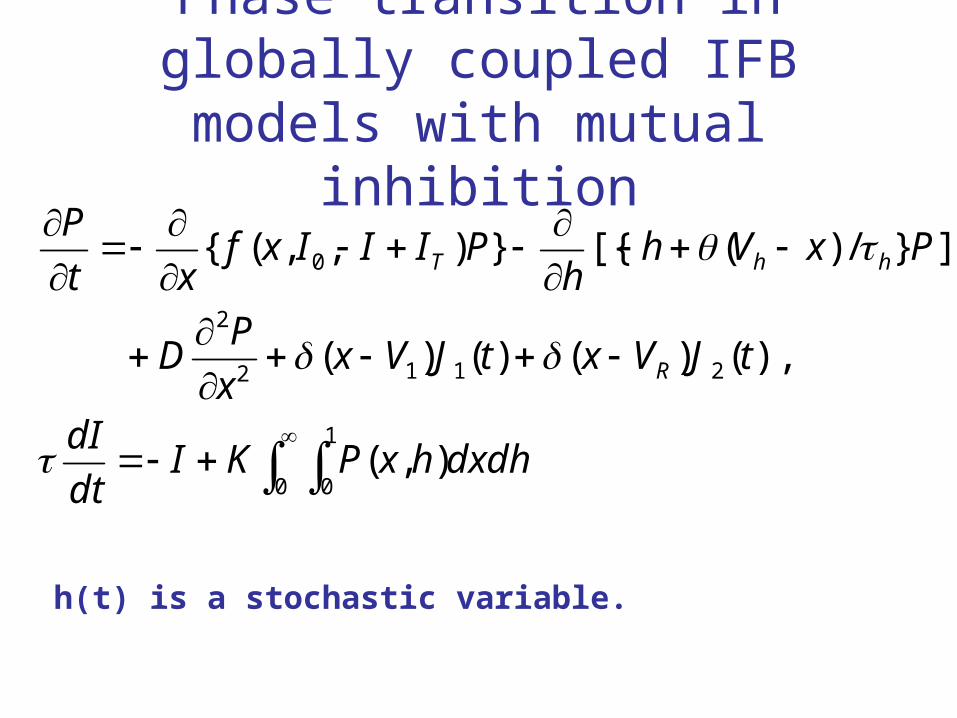
Phase transition in globally coupled IFB models with mutual inhibition
0
1
0
2112
2
0
),(
),()()()(
]}/)([{}),,({
dxdhhxPKIdt
dI
tJVxtJVxx
PD
PxVhh
PIIIxfxt
P
R
hhT
h(t) is a stochastic variable.

Bistability of globally coupled IFB model
I0=1.6,K=40, D=0.2 and τ=20.
h≠0, in one mode (rebound mode, burst mode).h=0, and IT does not work, in another mode (tonic mode).
Average membrane potential E(t) <h(t)> vs.I0.
Vh =-70I0 is external input
Two modes are bistable for 0.55<I0<2.2

Summary
1 Phase transition via mutual synchronization
2 Direct simulation of Fokker-Planck equation
3 Phase oscillator model and IF models
4 Transition to traveling wave states
5 Mutual synchronization in inhibitory systems Intermittent firing in strongly inhibited systems

Discussions and ProblemsGood points of the Fokker-Planck equation:
1. Stationary distribution might be solved.
2. Numerical results are clear, since it is
a deterministic equation.
Weak points of the Fokker-Planck equation:
If the number of stochastic variables is not one
or two, numerical simulations are rather hard.
Langevin simulations may be efficient for realistic equations such as noisy Hodgkin-Huxley equations.

References
Y.Kuramoto, “Chemical Oscillations, Waves
and Turbulence” Springer (Berlin, 1984).
H.Sakaguchi, Prog.Theor.Phys. Vol.79(1988) 39
S.H.Strogatz, Physica D Vol. 143 (2000) 1.
H.Sakaguchi, Phys.Rev. E Vol.70(2004) 022901.
M.Steriade and R.R.Llinas, Phsiol.Rev. Vol.68
(1988) 649