Study on improvement of ABS performance usingadditional sensor informationSteur, E.

Published: 01/01/2004

Document VersionPublisher’s PDF, also known as Version of Record (includes final page, issue and volume numbers)

Please check the document version of this publication:

• A submitted manuscript is the author's version of the article upon submission and before peer-review. There can be important differencesbetween the submitted version and the official published version of record. People interested in the research are advised to contact theauthor for the final version of the publication, or visit the DOI to the publisher's website.• The final author version and the galley proof are versions of the publication after peer review.• The final published version features the final layout of the paper including the volume, issue and page numbers.

Link to publication

Citation for published version (APA):Steur, E. (2004). Study on improvement of ABS performance using additional sensor information. (DCTrapporten; Vol. 2004.077). Eindhoven: Technische Universiteit Eindhoven.

General rightsCopyright and moral rights for the publications made accessible in the public portal are retained by the authors and/or other copyright ownersand it is a condition of accessing publications that users recognise and abide by the legal requirements associated with these rights.

• Users may download and print one copy of any publication from the public portal for the purpose of private study or research. • You may not further distribute the material or use it for any profit-making activity or commercial gain • You may freely distribute the URL identifying the publication in the public portal ?

Take down policyIf you believe that this document breaches copyright please contact us providing details, and we will remove access to the work immediatelyand investigate your claim.

Download date: 02. Jun. 2018

Study on improvement of ABS performance using additional

sensor information

E. Steur

DCT Report no: 2004.77 June 2004

TUIe Bachelor Final Project Report

Coaches: Dr. Ir. I.J.M. Besseling Dr. Ir. F.E. Veldpaus Ir. A.J.C. Schmeitz

Supervisor: Prof. Dr. Ir. M. Steinbuch

Eindhoven University of Technology Department of Mechanical Engineering Division Dynamical Systems Design Control Systems Technology

Eindhoven, June 25,2004

Abstract

In this report a quarter vehicle model is used to study the possibilities of improvement of the braking performance using additional sensor information. The model is implemented in Matlab-Simulink to simulate straight-line braking on both flat and uneven roads. The vehicle model includes a suspension model, a tyre model and models of Anti-lock braking systems.

A conventional ABS, based on combined wheel slip and wheel peripheral acceleration is compared with a new ABS controller using feedback linearization. Additional information for the feedback linearization is provided by so called "smart" sensorized tyres.

Simulation results are used to determine the benefits of using additional sensor information. The non-linear ABS controller seems to perform (much) better then a conventional ABS control algorithm.

Contents

Introduction 1.1 Historical overview 1.2 Objectives 1.3 Major components of ABS

Early Bosch B S algorithm 2.1 Typical control cycle

Quarter Vehicle Model 3.1 Vertical suspension 3.2 Horizontal suspension 3.3 Torque around the y-axis 3.4 SWIFT model 3.5 Parameters used in the Simulink Model

Tyre-to-road friction 4.1 Friction curves

Simulink model of a conventional ABS 5.1 Assumptions and restrictions 5.2 Slip computation block 5.3 Wheel peripheral acceleration block 5.4 The ABS block

Road and Tyre used in the simulations 6.1 Road 6.2 Tyre

Simulations with the Conventional ABS 7.1 Simulation results on a flat road 7.2 Simulation results on an uneven road 7.3 Simulation results on a wet road

Design of a non-linear ABS controller 8.1 Simplified QVM 8.2 Feedback linearization 8.3 Controller 8.4 Smart tyres and bearings

8.4.1 Smart tyres 8.4.2 Smart bearings

8.5 Reconstruction of F,, 8.6 The non-linear ABS block

Simulations with the non-linear ABS controller 9.1 Slip setpoint 9.2 Results of the simulations

10. Conclusion and Recommendations 10.1 Conclusion 10.2 Recommendations

References

Appendix A: SAE sign convention

Appendix B: QVM Si~~dkk Implemextaticn

Appendix C: M-file Conventional ABS

Appendix D: M-file non-linear ABS controller

Appendix E: Error in estimation of F,,

Appendix I;: Extended plots of the perfomaxce of the canventionalL4BS

Appendix G: Extended plots of the performance of the non-linear ABS

Appendix H: Performance of the non-linear ABS with a non-proper choice of K~

1 Chapter 2: Earlv Bosch Algorithm

Chapter 1

Introduction

An Anti-lock Braking System, briefly ABS, is an important component of a modern car. The ABS improves the braking performance of the vehicle compared to a conventional braking system by preventing wheel lock. When the brake torque, demanded by the driver through the pedai, will cause the wheeis to lock, the ABS takes over.

In a conventional ABS system, the wheel slip oscillates around a critical slip. The oscillation limits the ABS performance and has undesirable vibrations as side effect. A solution can be found in designing a more smooth, continuous controller whose setpoints are determined using information provided by wheel speed sensors and smart tyres and bearing.

This report is divided in two parts. First, a description of a Quarter Vehicle Model (QVM) and an ABS controller based on the early Bosch algorithm will be given, followed by its implementation in Simulink. Tine second part consists of a new, non-linear ABS control algorithm using some extra information provided by smart tyres and bearings. In both parts, the ABS controller will be evaluated for straight-line emergency braking on a flat and an uneven road.

1.1 Historical overview

The first ABS (Dunlop "Maxaret") was developed to assist airplanes to stop faster and along a straight line on slippery runways. The first automotive use of ABS was in 1954, when an ABS of a French aircraft was fitted on a limited number of Lincolns. In the late 60's Ford and Kelsey Hayes developed a rear-wheel-only ABS system for the Thunderbird. Chrysler and Bendix produced a four-wheel ABS for the Imperial in the early 70's. These systems used vacuum-actuated modulators and analogue electronics. Because the vacuum-actuated modulators cycled slowly and the electronics was not very reliable, the actual stopping distance even increased.

In Europe the major brake and electronics suppliers had decided to develop ABS, changing from analog to digital electronics and from vacuum to hydraulic actuation. In 1978 Mercedes used a Bosch hydraulic ABS on sedans. Audi and BMW followed. Japanese brake suppliers started to design their own ABS, based on the Bosch system. In 1985 Teves introduced the "integrated" ABS on the Lincoln Mark VII.

Today many cars are equipped with an ABS. By the late 80's ABS was offered on high-priced luxury and sports csrs. The modern ABS is s rtle bssed control system, using exhaustive tables for different braking scenarios, using criteria in terms of wheel peripheral acceleration 2nd wheel slip.

2 Chapter 2: Early Bosch Algorithm

1.2 Objectives

The objectives of an ABS are threefold.

Reduce the stopping distance The stopping distance is a function of the initial velocity, the mass of the vehicle and the brake force. Applying the brakes as hard as possible will not lead to the minimal stopping distance because it will cause the wheels to lock. Every tyre on nearly all types of surfaces will show a peak in the friction coefficient at a certain wheel slip. By keeping all of the wheels near the peak, maximum braking force will be achieved, and so the minimal stopping distance will be attained.

Improve stability Although maximal fiction will lead to the minimal stopping distance, not in all situations maximal friction is desirable. On so-called p-split surfaces (different friction condition for the left and right wheels), maximum friction on each wheel means that the braking force on the left will differ from that on the right, resulting in a jaw-moment. Select high and select low algorithms are introduced to maintain stability during braking on those p-split surfaces.

Improve steerability during braking The lateral force will decrease with increasing wheel slip. So with maximal wheel slip (locked wheel) the lateral force is almost equal to zero, and it is impossible to steer. Steerability during braking is important, for instance to avoid an obstacle during braking.

In each of these objectives the tyre characteristics play an important role. The longitudinal forces as well as the lateral forces are both generated within a small contact zone between the tyre and the road surface.

1.3 Major components of the ABS

The modern ABS in general consists of the following parts.

Wheel Speed Sensors These sensors are electro-magnetic pulse pickups with toothed wheels, mounted near the rotating components of the drive train or the wheel hub. These devices provide a digital signal whose frequency is proportional to the wheel rotational velocity.

Figure 1.1: wheel speed sensor (Bosch)

3 Chapter 2: Early Bosch Algorithm

Electronic Control Unit (ECU) The ECU is an electronic device containing signal processing units, computation functions and output devices. The (filtered) signals of the wheel speed sensors are used to estimate the vehicle velocity and to compute the wheel slip. When a wheel is going to lock, the ECU sends a signal to the brake pressure modulator to increase, hold or reduce the brake line pressure and hence the brake torque.

Brake Pressure Modulator The brake pressure modulator is an electro-hydraulic or electro-pneumatic device for increasing, holding or reducing the brake pressure. It modulates the brake pressure to one or more wheels, independent of the brake pedal actions of the driver. Depending on the design, this device nsly hclude 2 motorlpunp, accumu!Iltor 2nd reservoirs.

4 Chapter 2: Early Bosch Algorithm

Chapter 2

Early Bosch Algorithm

The basic control philosophy for a conventional ABS, is a combination of: wheel slip control and wheel peripheral acceleration control.

This type of control strategy is used in the eariy Bosch aigorithm. The reason for choosing wheel slip and wheelperipheral acceleration as control variables is that only wheel slip control or only wheel peripheral acceleration control gives satisfling performance: A combination of both can perform better.

Wheel slip as control variable Wheel slip is computed by the ECU using information from the wheel speed sensors. Because the tyre-road characteristics are highiy non-linear and road conditions are changing constantly, an ABS controller based only on wheel slip with a preset slip value will not always provide maximum braking force.

Wheel peripheral acceleration as control variable Wheel acceleration can be obtained by differentiating the angular velocity of the wheel. In case of high wheel moments of inertia, low friction coefficients and a slow rise of the brake pressure in the wheel brake cylinder (cautious initial braking, e.g. on black ice), the wheel might lock up without violating the acceleration threshold.

Combined wheel peripheral acceleration and slip as control variable Combining both control variables described above, nearly optimal control can be achieved.

2.1 Typical control cycle

The depicted control cycle in Figure 2.1 shows ABS control for high fiction coefficients. The wheel peripheral acceleration is computed in the ECU.

At the end of phase 1, when the value for the wheel peripheral acceleration drops below a preset threshold al, the hydraulic modulator valve unit is switched to the pressure hold mode. If afterwards the slip-switching threshold hl is exceeded as well, the valve unit is switched to pressure reduction. This will be done until the a1 threshold is crossed again. During the subsequent pressure holding phase, the wheel peripheral acceleration increases until the a2 threshold is exceeded; thereupon the pressure is kept constant. After the relatively high +A threshold is exceeded, the brake pressure is increased, to avoid excessive acceleration of the wheei as it enters the stabie range oftine fi-ictiodsiip curve. During phase 6, the pressure is maintained again at a constant level. After the a2 threshold is crossed, the brake pressure is slowly raised until, when the wheel peripheral acceleration falls below the a1 threshold, the second cycle is initiated, this time with an immediate pressure reduction. In the first cycle, the brief pressure holding phase 2 is necessary for the filtering of disturbances.

5 Chapter 2: Early Bosch Algorithm

Figure 2.1: Typical Control Cycle Posch)

6 Chapter 3: The Quarter Vehicle Model

Chapter 3

The Quarter Vehicle Model

To simulate a straight-line braking-manoeuvre a Simulink Quarter Vehicle Model (QVM) is used. This QVM is basically the same as in [pangelov, 20041. It includes a model of the suspension in vertical direction, a fore-aft axle compliance model, and a tyre (SWIFT) model (figure 3.1). The complete Simulink model of the Q W is given in Appendix B.

Figure 3.1: Quarter vehicle, suspension and tire representation in X and Z directions

3.1 Verticd suspension

In the vertical direction the suspension is modelled as a linear spring with stiffness k, and a linear viscous damper with damping c,. This spring-damper combination connects the vehicle body mass m2 with the unsprung-mass ml, consisting of the mass of all moving parts connected to the wheel hub such as the rim, the brake disc, the calliper etc. The equations of motion in the vertical direction are given by:

where 21 - vertical position of the unsprung-mass 22 - vertical position of the vehicle body mass Lo - the unloaded spring length

7 Cha~ter 3: The Quarter Vehicle Model

The vertical force F , , of the tyre on the rim is determined in the SWIFT model, using the road profile and the axle vertical position zl and velocity 2,.

Initially the system is at rest. The steady state position zlo of the axle and displacement zzo follow fiom:

where:

Yo - unloaded tyre radius

W o - initial road height

k,, - vertical tyre stiffness as specified in the SWIFT model.

3.2 Horizontal suspension

The equations of motions for the horizontal direction are given by:

The initial horizontal position xlo ofthe axle and xzo are set to zero.

3.3 Torque around the y-axis

The equation of motion for rotations around the y-axis is given by:

where I, - the wheel polar moment of inertia R, - wheel angular velocity

My,, - moment, exerted by the tyre on the rim Tb - brake torque

3.4 The Swift modei

The adopted tyre model used is the Short Wave Intermediate Frequency Tyre (SWIFT) model. The SWIFT model combines a Magic Formula slip force description with a rigid ring for the thread. This rigid ring is suspended to the rim by a vertical and longitudinal sidewall stiffness kb and damping cb. Rotational sidewall stiffness and damping are included as well in the model. The contact model uses the spring stiffhess k,, to model the vertical force at the contact point (Figure 3.2). Experiments show that the total vertical stiffness of the tyre is smaller then the stiffness kb of the first mode of vibration. To match the vertical s t i ~ e s s of

8 Chapter 3: The Quarter Vehicle Model

the model with the real tyre, the residual stiffness k,, is introduced. More information about the SWIFT model can be found in [TNO automotive, 20021.

Figure 3.2: Side view of the rigid-ring representation of the tyre. In-plain characteristics.

3.5 Parameters used in the Simulink model

Table 3.1: values used in the Simulink model

Velocity at which the vehicle is considered stopped Wheel-tire assemble polar moment of inertia Unloaded tire radius Effective rolling radius Vehicle initial velocity Maximum value of the brake torque

ustop

ID TO

ref U,,

Tb,max

1 .o 1 .04

0.3 135 0.3067

variable 2500

mls

kg.m2 m m m/s Nm

9 Chapter 4: Tvre-to-road friction

Chapter 4

Tyre-to-road friction

ABS control involves uncertainties, mainly due to the highly non-linear and uncertain tyre-to- road friction characteristics. A commonly used model for this friction is the "magic formulayy or Pacejka model [Pacejka, 20021. In this work a Pacejka model be used for simulations.

4.1 Friction curves

The tyre-to-road friction p is a non-linear function of: K - longitudinal wheel slip; a - slip angle of the wheel; p~ - maximum friction coefficient between tyre and road; F, - vertical force,

The longitudinal friction force F, is given by

Where the longitudinal wheel slip K is defmed as:

U U

with u - the velocity of the wheel centre in x-direction; us - the longitudinal slip speed. (us = u - Q, rg); ref/. - the effective rolling radius of the tyre.

The slip value K = 0 characterizes the free motion of the wheel, i.e when no longitudinal friction force is exerted. When K = -1, the wheel is fully locked (SZ, = 0 ) and the friction coefficient will be reduced to p~ (Figure 4.1).

The friction coefficient will reach its maximum p~ for the optimal longitudinal wheel slip KO.

For values of K < KO, the friction coefficient enters the unstable region. Any further increase in slip within this region will lead to a decrease in p.

The friction coefficient highly depends on the road surface (see figure 4.1) [Dijks, 19741. Some typical ambers are given in Table 4.1.

Table 4.1: pn and p~ for different types of roads

I Ice -0.22 -0.07 1

Road surface Asphalt (dryl Amhalt (wet)

PH -1.21 -0.85

PG -0.81 -0.44

10 Chapter 4: Tyre-to-road friction

-1.5 -1 -0.9 -0.8 -0.7 -0.6 -0.5 -0.4 -0.3 -0.2 " ~ 0 . 1 0

K 1-1

-0.5

Fz=5kN . . . . Fz=9kN

-1.5 -1 -0.9 -0.8 -0.7 -0.6 -0.5 -0.4 -0.3 -0.2 -0.1 0

. . . . . . . . . . ........

- A 3

- . . . . ice

-1.5 -1 -0.9 -0.8 -0.7 -0.6 -0.5 -0.4 -0.3 -0.2 -0.1 0

Figure 4.1: typical friction curves

I=.-.-.- -:--.-i:- - _ - _ _ - ...... . /

.................... ....

--- a = 3 deg

, .. - a = I deg --- - - I

--- a = 3 d e g a = 7 d e g

- - a = 10 deg I I I I I I I I I

-0.9 -0.8 -0.7 -0.6 -0.5 -0.4 -0.3 -0.2 -0.1 0 K 1-1

Figure 4.2: Tyre side slip friction curves

11 Chapter 5: Sirnulink Model of a Conventional ABS

Chapter 5

Simulink model of a conventional ABS

The conventional ABS is based on the early Bosch algorithm and the combined slip and wheel peripheral acceleration controller presented in [Rangelov, 20041.

5.1 Assumption and Restrictions

a Only straight-line braking until a pre-set stop velocity is reached is considered. a The ABS is not operational for velocities below 1 mls.

Rates of the brake torque increase and decrease are fmed. At each time t the wheel angular velocity R and the vehicle longitudinal velocity U are available from measurements andlor reconstruction.

a The brake torque is realised without any time delay; Effects of hydraulics will be neglected.

a The effect of load transfer during braking will be neglected.

5.2 Slip Computation Block

The longitudinal slip, given by equation 4.2, is computed in the slip computation block. The comparator outputs a "1" when the slip threshold is exceeded.

r kappa I S l i ~ Threshold

U(4 YU(2) - 1

X2-dot Slip Computation

(double)

Slip threshold Relational Data Type Conve Operator

Figure 5.1 Slip Computation Block

5.3 Wheel Peripheral Acceleration Block

The wheel peripheral acceleration a,,, is computed according to:

where h, - the angular acceleration of the rim

In the block comparators are introduced, which outputs a "1" when a threshold (al, a2 or A) is exceeded.

12 Chapter 5: Simulink Model of a Conventional ABS

derivative/ L o w p a n filter

Data Type Conversion1

Omega Operator

u Wheel Aooel./Deceleration

A threshold (double)

- - - Relational Data Type Conversion2 *

a2 threshold

a? threshold Relational OperatoR

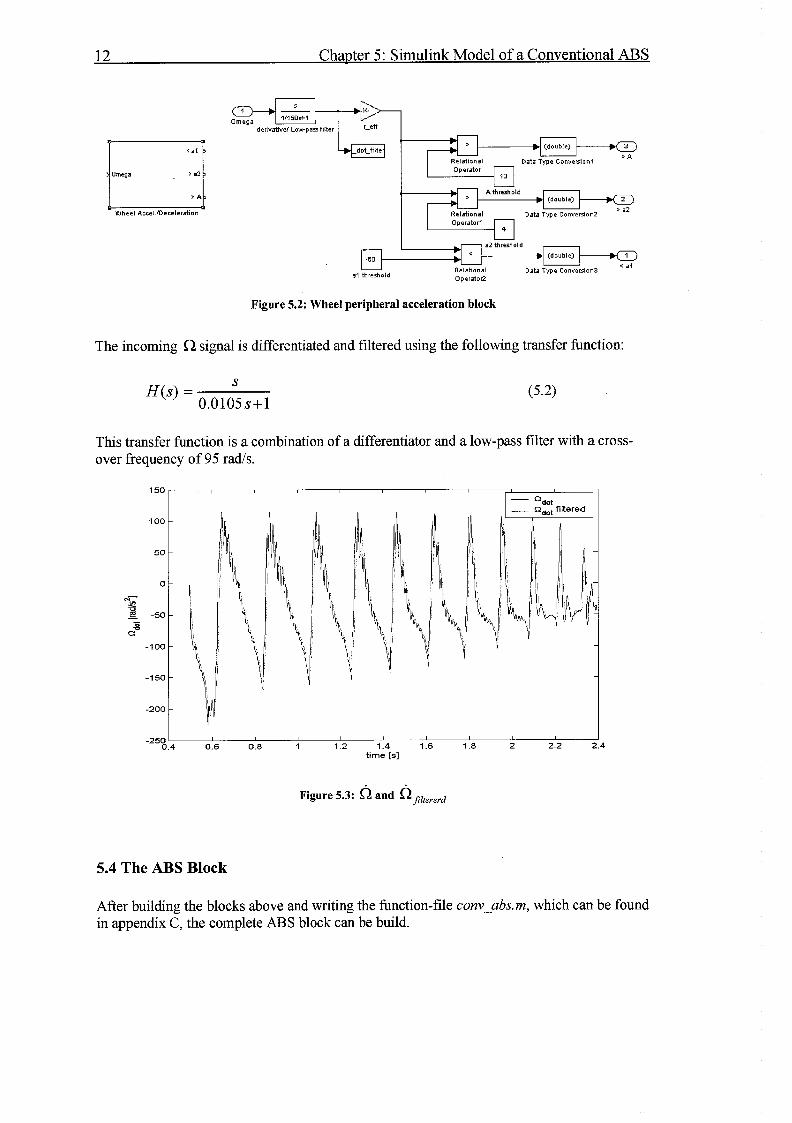
Figure 5.2: Wheel peripheral acceleration block

The incoming R signal is differentiated and filtered using the following transfer function:

This transfer function is a combination of a differentiator and a low-pass filter with a cross- over frequency of 95 radls.

-250 I I , I I I I I I

0.4 0.6 0.8 1 1 .2 1.4 1.6 1.8 2 2.2 2.4 time [s]

Figure 5.3: fi and Rfiltererd

5.4 The ABS Block

After building the blocks above and writing the function-file convabxm, which can be found in appendix C, the complete ABS block can be build.

13 Chapter 5: Sirnulink Model of a Conventional ABS

Brake-appl

omega I-1 ABS b l o d

Omega > aZ t. MATLAB Fundion

MATLAB Fcn Integrator ,A t.

I I Wheel Accel./Deceleratlon

Omega

c kappa

Slip Threshold

Figure 5.5: Complete ABS Block

As mentioned before, the rates of increase of the brake torque are fixed. The values used are given in Table 5.1.

Table 5.1: values of Rl-fast, Rl-slow and R2

R1 fast, rate of increase of the brake torque fast R1 slow, rate of increase of the brake torque slow R2, rate of decrease of the brake torque

19000 N d s 2533 N d s - 19000 N d s

14 Chapter 6: Road and Tvre used in the Simulations

Chapter 6

Road and Tyre used in the Simulations

The QVM with ABS will be simulated on two different high friction roads.

6.1 Road

The simulations are performed for a completely flat road and a very uneven road. Both roads have a surface of asphalt (dry or wet). The picture below shows the characteristics of the used uneven road.

left track data 0.3 I I I I I I I I I

-0.2 1 I I I I I I I I I I 0 100 200 300 400 500 600 700 800 900 1000

travelled distance [m]

right track data 0.3 I I I I I I I I I

-0.2 1 I I I I I I I I 1 I 0 100 200 300 400 500 600 700 800 900 1000

travelled distance [m]

Figure 6.1: characteristics uneven road; travelled distance versus road height

Figure (6.2) shows the forces in the z-direction acting on the rim and in the tyre-road contact point at a constant velocity of 80 W h . The brakes are applied after 3.5 seconds, when the tyre is hardly contacting the road.

15 Chapter 6: Road and Tyre used in the Simulations

01 I I I I I 0 1 2 3 4 5

time [s]

Figure 6.2: Contact force FGC versus time, driving on a uneven road without braking

6.2 Tyre

The tyre is a standard passenger car tyre of type 205/60R15, where (see Figure 5.2):

205 - section width of the tyre in millimetres. 60 - aspect ratio: the ratio between the section height and section width in %. R - construction of the tyre: radial tyre. 15 - diameter of the rim in inches.

outer diameter

j section j height

* - ' rim diameter

Pignre 5.2: The tyre cross-section

16 Chapter 7: Simulations with the Conventional ABS

Chapter 7

Simulations with the Conventional ABS

The conventional ABS is tested in simulations with an initial velocity of 80 W h .

The theoretical minimal stopping distance and the stopping distance with fully locked wheels on a dry and on a wet road are given in the table below.

Table 7.1: stopping distances for a car with an initial velocity of 80 km/h on a high friction road

I Fully locked (wet road) 57.01

Theoretical minimum (dry road) Fully locked (dry road) Theoretical minimum (wet road)

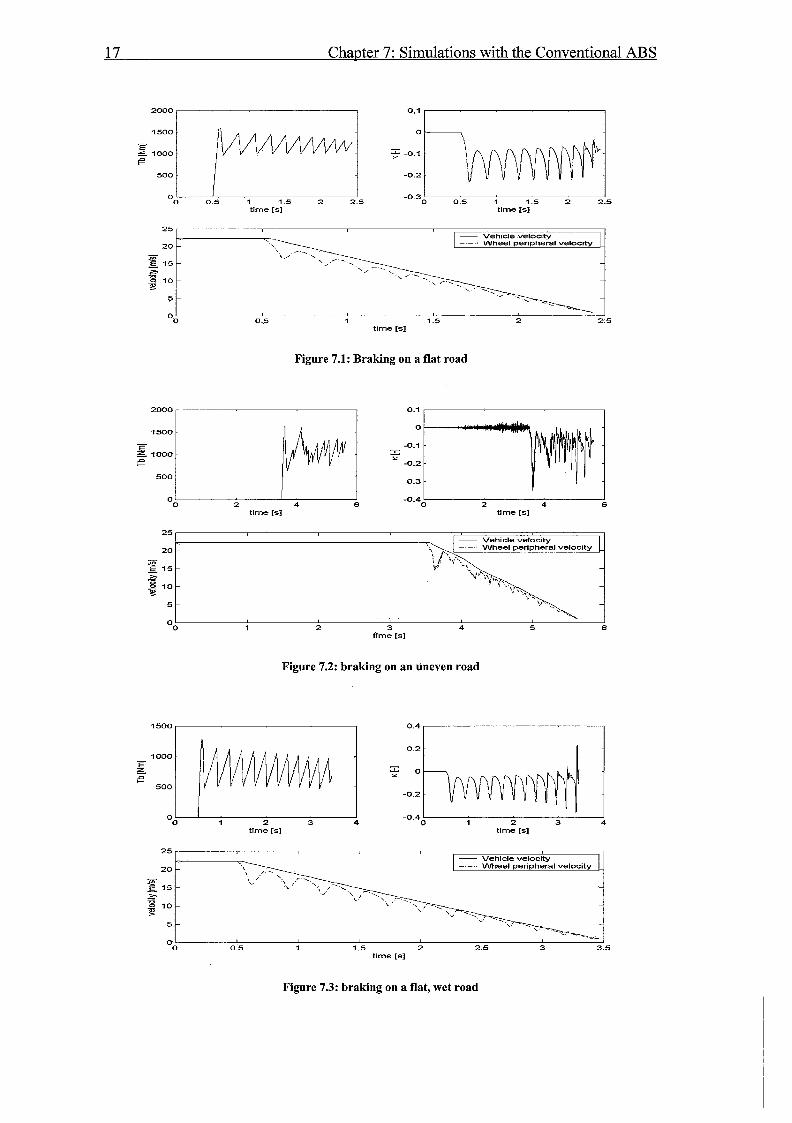
7.1 simulation results on a flat road

20.66 31.14 29.52

Figure (7.1) shows the results of the ABS on a flat road. The thresholds used, provided by [Rangelov, 20041, are given in Table 7.2.

Table 7.2: used theshold values

With these values of the thresholds, the stopping distance is 22.65 m, implying a large influence of the ABS.

Slip a1 a2

7.2 simulation results on a uneven road

20 % - 60 rn/s2 4 rn/s2

The simulation on the uneven road with the use of the same thresholds is depicted in figure (7.2). The brakes are applied after 3.5 s (see Section 6.1), which results in a stopping distance of 25.43 m.

7.3 simulation results on a wet road

Finally, simulations are performed on a flat, wet road (see Figure 7.3). The stopping distance yields 33.91 m, there the theoretical minimum yields 29.52 m.

Appendix F will show more extended plots of the performance of the conventional ABS.

17 Chapter 7: Simulations with the Conventional ABS

0.5 1 1.5 2 2.5 time [s]

2000

1500 - E 2 1000 e

500

0

Figure 7.1: Braking on a flat road

I . I 2 4 6 2 4

-0.4

time [s] time [s]

0 05 1 15 2 25 -0 3

0 05 1 15 2 25 tlme Is] tune [sl

-

-

-

5

0 1 2 3 4 5 6

time [s]

0 1

0

- " -0 1 -0 2

Figure 7.2: braking on an uneven road

0.2 - 1000 E - z A

e r 0

500 -0.2

0 1 2 3 4 1 2 3

-0.4

time Is] time [s]

Vehlcle veloclty Wheel per~pheral velocity

E \ - B 10 9

5

0 5 1 15 2 2 5 3 3 5 tlme [s]

Figure 7.3: braking on a flat, wet road

18 Chapter 8: Design of a non-linear ABS Controller

Chapter 8

Design of a nonlinear ABS controller

8.1 Simplified QVM

For the design of a non-linear controller, a simplified QVM will be used (see Figure 8.1).

Figure 8.1: Simplified QVM

The equations of motion are given by:

where m - total mass of the QVM

Using the longitudinal wheel slip definition (equation 4.2), the derivative of the slip can be written as:

Here it is assumed that the derivative of the effective radius refmay be neglected.

19 Chapter 8: Design of a non-linear ABS Controller

8.2 Feedback linearization

The non-linearity of equation 8.3 can be cancelled using feedback linearization. For that purpose equation 8.3 is written as:

1 1 K = - - ~ ( K ) - - c T ~ U U

Now let Tb be:

where Tbcontro, = U P(K - Kd )- U K~

with m the desired wheel slip (setpoint). We will assume this slip setpoint will be provided by a higher level control system such as an ESP (Electronic Stability Program).

The tracking error of the closed loop system is given by:

e+Pe =O (8.7)

which yields exponential convergence of e (= rc - red) to zero.

8.3 Controller

For the sake of simplicity a P-controller is chosen (see equation 8.6). The control gain P is multiplied with the vehicle velocity u to eliminate the velocity in the error equation 8.7.

8.4 Smart tyres and bearings

The use of this control law requires extra information about the longitudinal force in the contact point F,. This extra information might be gathered using smart tyres and/or smart bearings.

8.4.1 Smart tyres

Smart tyres provide information of the moment My,, exerted by the lyre on the rim (see figure 3.1). This so called Sidewall Torsion (SWT) system is able to estimate My,, by measuring defamation of the side wa!! using a semor (see figure 8.2, number 1) md some rnqp3 . i~ strip (see figure 8.2, number 2).

20 Chapter 8: Design of a non-linear ABS Controller

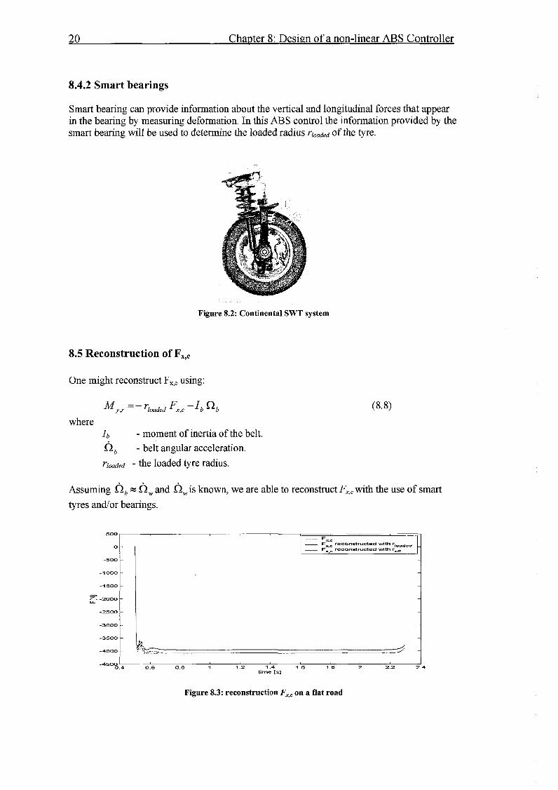
8.4.2 Smart bearings

Smart bearing can provide information about the vertical and longitudinal forces that appear in the bearing by measuring deformation. In this ABS control the information provided by the smart bearing will be used to determine the loaded radius rlOaded of the tyre.

Figure 8.2: Continental SWT system

8.5 Reconstruction of F , ,

One might reconstruct F,, using:

My,i- =- 'loaded Fx,c -I6 ab

where I b - moment of inertia of the belt.

- belt angular acceleration.

rladed - the loaded tyre radius.

Assuming = hw and hw is known, we are able to reconstruct F,, with the use of smart

tyres andor bearings.

Fx.s - FX.= reconstructed wlth r

I F,,, reconstructed woth r,*

I 0.6 0.8 1 1.2 1.4 1.6 1 .8 2 2.2 2.4

time [q]

Figure 8.3: reconstruction F , , on a flat road

2 1 Cha~ter 8: Design of a non-linear ABS Controller

- FXe reconstructed with rloeded

I I I

3.6 3.8 4 4 2 4.4 4.6 4.8 5 5.2 time [s]

Figure 8.4: reconstmctian Fx,, on a uneven road

Fx,, is reconstructed with the use of rloaded and reff instead of r loakd (see figure 8.3, figure 8.4 and appendix E). Both results are satisfying. From a economic point we will reconstruct F, , with the use of ref instead of r l d e d , SO only smart tyres are needed.

8.6 The non-linear ABS Block

The control law (equation 8.5) is provided in an m-file, which is presented in appendix D. The signals My,, and fl, are filtered using first order low-pass filters with a cross-over frequency

of 200 rad/s and 10 rad/s, respectively

omega

Brake-appl -EB9 zero Switch Saturation

Figure 8.5: ABS block non-linear controller

22 Chapter 9: Simulations with the non-linear ABS Controller

Chapter 9

Simulations with the nonlinear ABS controller

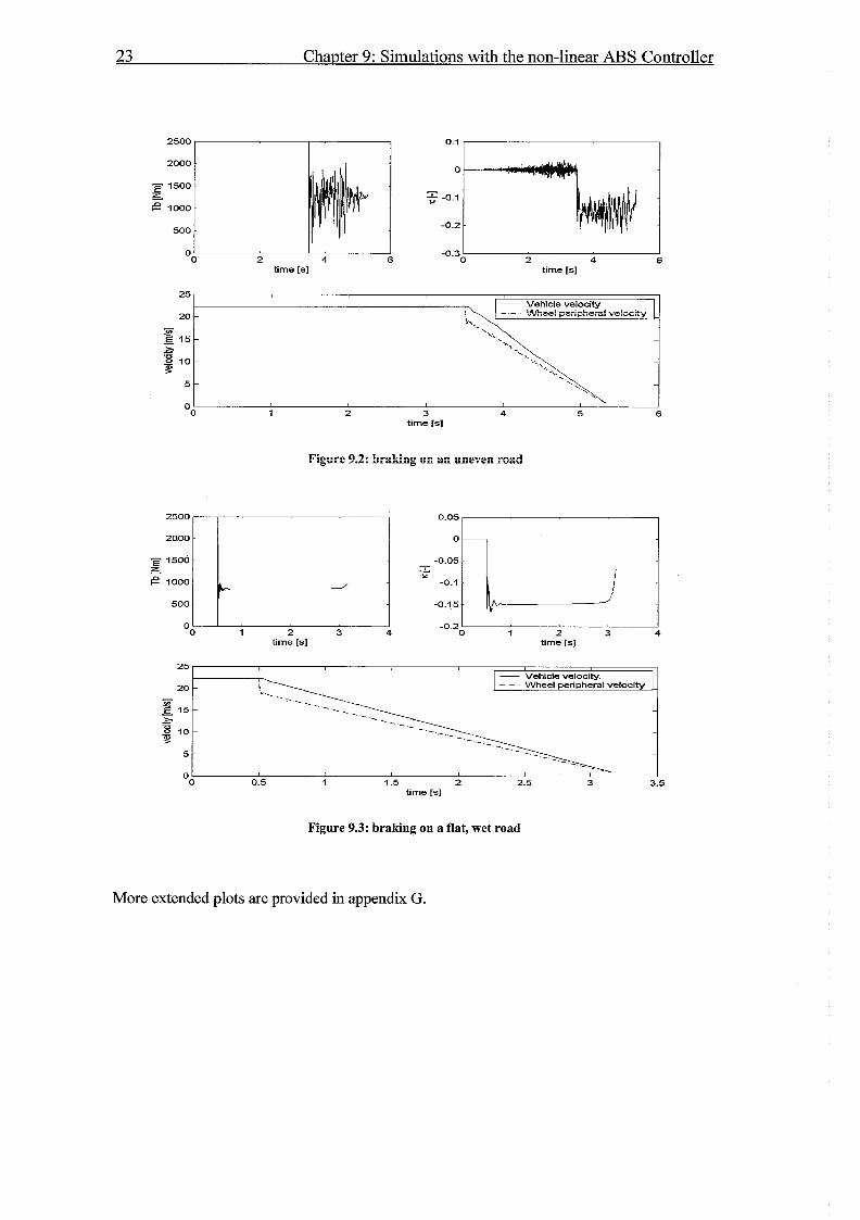
Like the conventional ABS the performance of the nonlinear ABS controller is tested using simulations on a dry or wet flat road, and on an uneven road for an initial velocity of 80 km/h.

9.1 Slip setpoint

The setpoint of the longitudinal wheel slip ~d is set at -0.15. At this value maximum friction will be achieved for the dry road (see figure 4.1). The gain P is determined empirically and is set to 300 Nm.

9.2 Results of the simulations

The stoppings distances on the flat road, the uneven road and on the wet road are presented in table 9.1.

Table 9.1: stopping distances with the non-linear ABS

A non-proper choice of the slip setpoint ~ d ( ~ d = -0.20 for example), when the unstable region of the friction curve will be entered, will not result in unstable behavior of the ABS (see figure HI, appendix H). Only with a extreme high gain (P = 3000 for example), the dynamics will become unstable (see figure H2), probably due to the difference between the simulation model and the control design model.

Flat road (dry) Uneven road (dry) Flat road (wet)

I I I -0.2 1 I '0 0.5 1 1.5 2 2.5 0 0.5 1 1.5 2 2.5

time [s] time [sl

Stopping distance [m] 20.94 21.24 30.94

Figure 9.1: braking on an flat road

23 Chapter 9: Simulations with the non-linear ABS Controller

2500 0.1

2000 0

I500 - 3 A -0.1 i= 1000

500 -0.2

0 0 2 4 6 0 2 4 6

-0.3

time [s] time [s]

time [s ]

25

20 - g 1 5 -

0 8 10- - S

5

0

Figure 9.2: braEng on an uneven road

- Vehlcle veloclty - W e e : peripheral ve:oci:y

-

-

- -

8 I

1 2 3 4 5 6

2500

2000

= 1500 3 e 1000

500

time [s]

Figure 9.3: braking on a flat, wet road

-- 20 -

e E 15- - )1 = 8 10- - Y

5

0

More extended plots are provided in appendix G.

-

-

- /

-

- Vehlcle veloclty - - - Wheel per~pheral velocity

-

-

- -

0.5 1 1.5 2 2.5 3 3.5

0.05

- L Y

Oo 1 2 3 4 1 2 3 -0.2

tlme [s] time [s]

24 Chapter 1 0: Conclusions and recommendations

Chapter 10

Conclusions and Recommendations

10.1 Conclusions

The design and implementation of a simple but accurate non-linear ABS controller is presented. The performance of this controller is much better than the performance of a conventional ABS (see figure 10.1). The use of additional sensor information (smart tyres) is beneficial.

Locked wheel braking

Conventional ABS

Nonlinear ABS controller

Theoretical minimum

flat road (wet)

684 uneven road (dryl

!&Ti flat road (dryl

Figure 10.1: comparison of stopping distance in meters with the different ABS

10.2 Recommendations

In order to improve the braking performance further study of the wheel lock criteria and braking algorithms is necessary.

First the stability and robustness of the non-linear ABS controller should be investigated in more detail.

The use of a PI controller in combination with feedback-linearization might even perform better then a P controiler in combination feedback-linearization. The effect of load disturbances is minimized due to I-action [Solyom 20021.

Studies on adaptive control technologies like extremum-seeking control might be beneficial in the ABS control problem. This type of control is able to find the maximum or minimum of an opthisation function if that function has a maximum or minimum. More information can be found in [Ariyur, 20021 and [Ariyur, 20031.

25 References

References

Besselink, I.G.M. (2003). Vehicle Dynamics, Lecture Notes, Eindhoven University of Technology, the Netherlands.

Bosch, Robert (2000). Bosch Automotive Handbook, 51h edition. Society of Automotive Engineers, Warrendale P.A.

Dijks, A (1974). A mudtvactor examiaatioa ofwet $.kid resistaace o f cw tyes. Society of Automotive Engineers, Warrendale P.A.

Ariyur,K. B. and Krstic.M (2002). Multivariable Extremum Seeking Feedback: Analysis and Design. Department of Mechanical and Aerospace Engineering University of California, San Diego.

Ariyur, K.B (2003). Real-time Optimalization by Extremum-Seeking Control. John Wiley & Sons hc.

Pacejka, H. B. (2002). Tyre and Vehicle Dynamics. Butterworth-Heinemann, Oxford.

Peterson, Idar (2003). Wheel Slip Control in ABS Brakes using Gain Scheduled Optimal Control with Constraints. Norwegian University of Science and Technology Trondheim, Norway.

Rangelov, Kiril Z. (2004). SIMULINK Models of a Quarter-Vehicle with an Anti-lock Braking System. Eindhoven University of Technology, the Netherlands.

Rowell, J. Martin and Paul S. Gritt (1 987). ANTI-LOCK BRAKING SYSTEMS for Passenger Cars and Light Trucks - A Review. Society of Automotive Engineers, Warrendale P.A.

Slotine, J. J. and W. Li (2002). Applied Nonlinear Control. Prentice Hall, Englewood Cliffs, New Jersey.

Solyom,S (2002). Synthesis of a Model-based Tire Slip Controller. Department of Automatic Contro1,Lund Institute of Technology. Lund, Sweden

The Mathworks (2003). Matlab Release 13 service pack I documentation.

TNO Automotive (2002). Delft Tyre -Tyre models user Manuel. Delft, The Netherlands.

TNO Automotive (2003). Matlab/Simulink Installation and User Manual. Delft, The Netherlands.

26 Appendix A: SAE Sign Convention

Appendix A

SAE Sign Convention

The vehicle axis system used in this report is consistent with the SAE sign convention.

Yaw Velocity (r)

z Axis

Figure Al: SAE sign convention

vehicle x,y,z axis system x: pointing forward, through plane of symmetry y: pointing sideward, normal to plane of symmetry z: normal to the road x,y: parallel to the road

translation x-direction: longitudinal velocity u y-direction: lateral velocity v z-direction: vertical velocity w

rotation x-direction: roll velocity p y-direction: pitch velocity q z-direction: yaw velocity

27 Appendix B: OVM Simulink Implementation

Appendix B

QVM Simulink Implementation

The QVM basically consists of three different parts: vertical suspension

horizontal suspension axle-tyre-road system

Vertical suspension The Simulink model of the horizontal suspension is made using equations 3.1 and 3.2.

Figure B1: Simulink representation of the vertical suspension

Horizontal suspension The Simulink model of the horizontal suspension is made using equations 3.5 and 3.6.

suspension

zero veloeihr

switch integrator stopping

I Distance

Figure B2: Simulink representation of the horizontal suspension

28 Appendix B: QVM Simulink Implementation

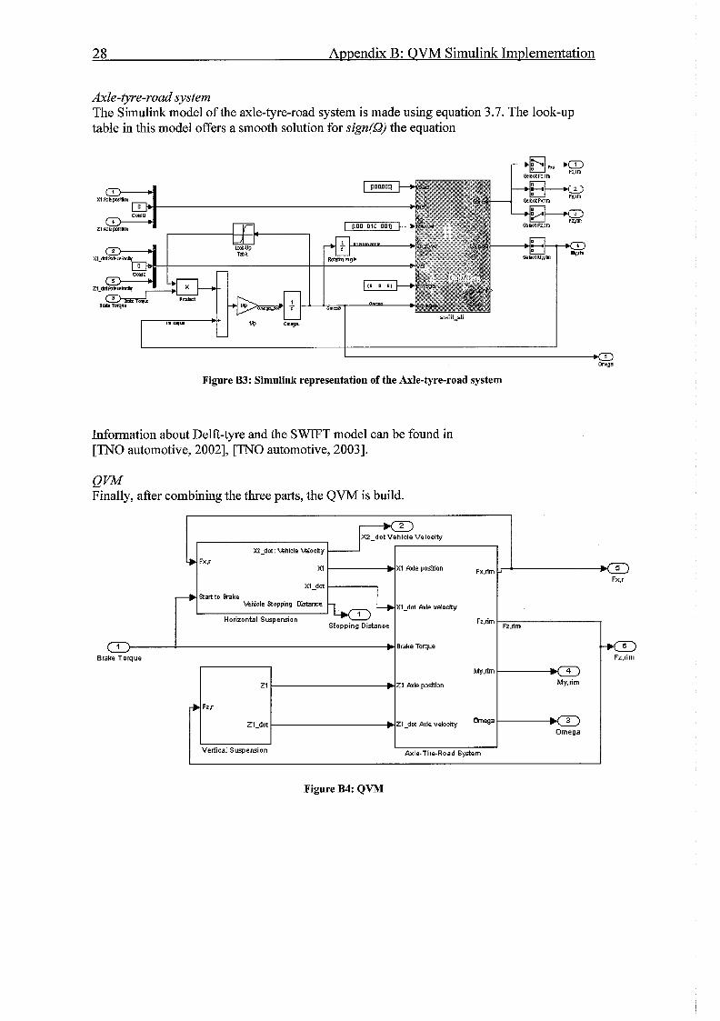
Axle-tyre-road system The Sirnulink model of the axle-tyre-road system is made using equation 3.7. The look-up table in this model offers a smooth solution for sign(S2) the equation

I a omega

Figure B3: Simulink representation of the Axle-tyre-road system

Information about Delft-tyre and the SWIFT model can be found in [TNO automotive, 20021, [TNO automotive, 20031.

QVM Finally, after combining the three parts, the QVM is build.

XI 1 2 ~ 1 ale position

XI-dot Stan to Brake

Xl-dot Pale velocity

Horizontal Suspension

Brake Toque

Brake Torque

X2-dot vehicle Velocity

I

- I Vedical Suspension I

Axle-Tire-Road System

Fx.rim

Fz.rim

W.rim

Omega

My.rim

Omega

Figure B4: QVM

29 Appendix C: M-file Conventional ABS

Appendix C

M-file Conventional ABS

% file: conv-abs.m

% This function computes the increase/decrease of the brake torque % according to some preset threshold values. The effects of hydraulics are % neglected. This file is only suitable for simulations of emergency braking % manoeuvres.

% INPUTS: % brake-appl The command "brake-appl" denotes when the brakes are 5. applied. % al-exceeded gives 1 if preset a1 is exceeded, 0 if not % a2-exceeded gives 1 if preset a2 is exceeded, 0 if not % A-exceeded gives 1 if preset A is exceeded, 0 if not % slip-exceeded gives 1 if preset slip is exceeded, 0 if not

%OUTPUT : %dTb Rate of increase or decrease or hold of the brake torque.

function dTb = conv-abs(brake-appl, al-exceeded, a2_exceeded, A-exceeded, slip-exceeded);

% defining global variables global n k dTb

% rates in increase/decrease Rl-f = 19000; % Fast rate of increase of the brake torque. Rl-s = 2533; % Slow rate of increase of the brake torque.

% This rate of increase replaces the modulated increase % of the brake torque in the Bosch algorithm.

R2 = -19000; % Rate of decrease of the brake torque.

% Algorithm: The algorithm is build using switch cases (Thresholds). % The variable "n" denotes the different parts of the typical control cycle. % The variable "k" is used as a first cycle indicator.

if brake-appl == 1, switch 1, case n == 1 & k == 0 & al-exceeded == 1,

dTb = 0; n = 2; case n == 1 & k == 1 & (al-exceeded == 1 I slip-exceeded == I),

dTb = R2; n = 3; case n == 2 & slip-exceeded == 1,

dTb = R2; n = 3; case n == 3 & a2-exceeded == 1,

dTb = 0; n = 4; case n == 4 & A-exceeded == 1,

dTb = Rl-s; n = 5; case n == 5 & A-exceeded == 0,

dTb = 0; n = 6; k = 1; case n == 6 & k == 0 & a2-exceeded == 0,

dTb = Rl-f; n = 1; case n == 6 & k == 1 & a2-exceeded == 0,

dTb = Rl-s; n = 1; otherwise

dTb = dTb; n = n; end

else dTb = R2; n = 6; k = 0;

end

3 0 Appendix D: M-file nonlinear ABS Controller

Appendix D

M-file non-linear ABS Controller

% m-file Tbcontro1.m

% This function computes the brake torque according to the non-linear % control law. The effects of hydraulics are neglected. % This file is only suitable for simulations of emergency braking % manoeuvres.

% INPUTS: % brake-appl The command "brake-appl" denotes when the brakes are applied. % x2-dot Vehicle velocity % omega wheel angular velocity % omega-dot wheel angular acceleration % My-r Moment exerted by the yre on the rim

%OUTPUT : % Tb Brake Torque

function Tb = Tbcontrol(x2_dot, omega, omega-dot, My-r)

% constants I-belt = 0.695; %[kg.mA21 Moment of inertia of the belt I-wheel = 1.04; %[kg.mA21 Moment of inertia of the wheel m = 335; %[kg] Mass of the QVM r-eff = 0.3067; % [m] The effective tyre radius c = r-eff / I-wheel;

% controller variables P = 300; % Gain kappa-des = -0.15; % desired slip

% computation wheel longitudinal slip kappa = omega * r-eff / x2-dot - 1;

% approximation of Fx-c using additional sensor information Fx-approx = -(My-r + I-belt * omega-dot) / r-eff;

% computation £(kappa) f = ( l/m * (1 + kappa) + (r-effA2) / I-wheel ) * Fx-approx;

% computation Tb ~b = -l/c*f + x2_dot/c * P * (kappa - kappa-des);

3 1 Appendix E: Error in estimation of F'

Appendix E

Error in estimation of Fx,c

estimation of F,,, uslng rloaded 0.02 I I I I I I I ,

Mean: 0.000282 Standard deviation 0.006i52

-0.06 I I I I I I I I I 0.4 0.6 0.8 1 1.2 1.4 1.6 1.8 2 2.2 :

time [s]

estimation of F,,, using reR

2 -0.04 aa

-0.06 Mean: -0.031 127

e! Standard deviation 0.006020

time [s]

Figure El: Error in estimation F , , on a flat road

estimation of F,,, using rloaded I I I I I I I I I I

estimation of F,,, using raw

-1

1

0.5 - - g 0

B 4 -0.5 - e!

-1

-1.5 3.4 3.6 3.8 4 4.2 4.4 4.6 4.8 5 5.2 5.4

time [s]

- 1 Mean: -0.00071 6 Standard deviation 0.149530

Figure E2: Error in estimation FX,C on an uneven road

-1.5 I I I I I I I I I

3.4 3.6 3.8 4 4.2 4.4 4.6 4.8 5 5.2 ! time [s]

3 2 Appendix F: Extended plots of the performance of the conventional ABS

Appendix F

Extended plots of the performance of the conventional ABS

I I I I

t - 7 - 7 d o d o

Figure F1: Conventional ABS; braking on a flat road

3 3 Appendix F: Extended plots of the performance of the conventional ABS

Figure F2: Conventional ABS; braking on a uneven road

3 4 Appendix - F: Extended plots of the performance of the conventional ABS

Figure F3: Conventional ABS; braking on a flat, wet road

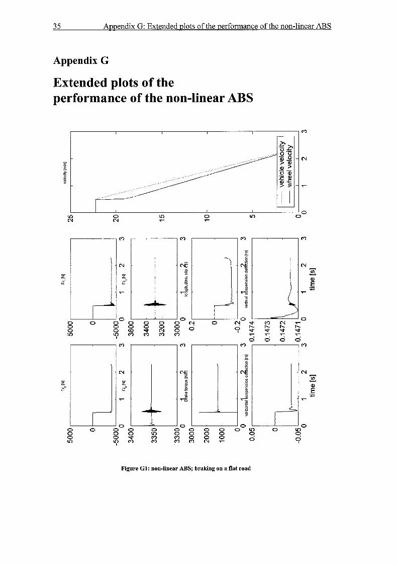
35 Appendix G: Extended plots of the performance of the non-linear ABS

Appendix G

Extended plots of the performance of the non-linear ABS

Figure GI: non-linear ABS; braking on a flat road

36 Appendix G: Extended plots of the performance of the non-linear ABS

Figure G2: non-linear ABS; braking on an uneven road

37 Appendix G: Extended plots of the performance of the non-linear ABS

Figure G3: non-linear ABS; braking on a flat, wet road

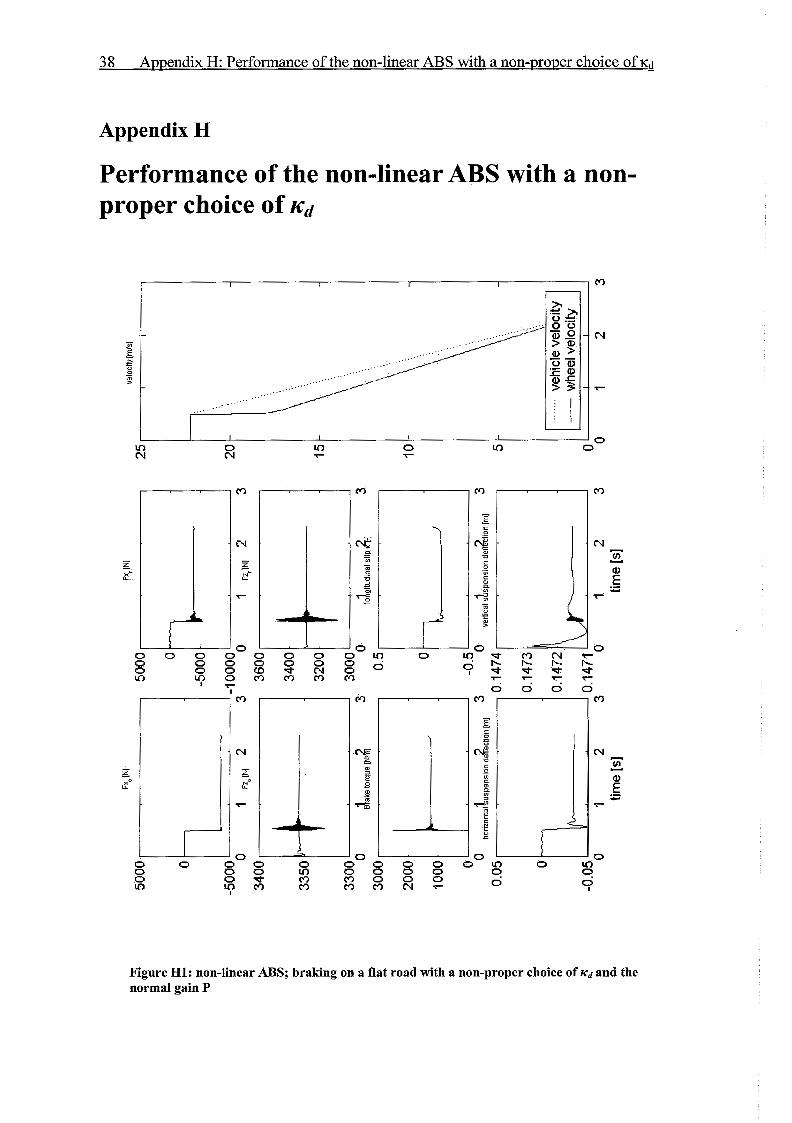
38 Appendix H: Performance of the non-linear ABS with a non-proper choice of K~ -

Appendix H

Performance of the non-linear ABS with a non- proper choice of

Figure HI: non-linear ABS; braking on a flat road with a non-proper choice of I C ~ and the normal gain P

39 Appendix H: Performance of the non-linear ABS with a non-proper choice of K~

Figure H2: non-linear ABS; braking on a flat road with a non-proper choice of red and an exteme high gain P