Study on Hysteresis Model of Welding Material in ...

applied sciences

Article

Study on Hysteresis Model of Welding Material inUnstiffened Welded Joints of Steel TubularTruss Structure

Yaqi Suo 1 , Wenwei Yang 1,* and Peng Chen 2

1 College of Civil and Hydraulic Engineering, Ningxia University, Yinchuan 750021, China; [email protected] Institute of Architectural Engineering, Huangshan University, Huangshan 245021, China; [email protected]* Correspondence: [email protected]

Received: 27 August 2018; Accepted: 16 September 2018; Published: 19 September 2018��

Featured Application: The main purpose of this study is to present a damage constitutive modelof welded joints in steel structures, which can provide a basis for the precise design of steelstructure joints. It can be popularized and applied in steel structure building, hydraulic steelstructure pump house, dike and so on in field of civil engineering and hydraulic engineering.It also can be used for reference in the field of mechanical manufacturing.

Abstract: The weld form of intersecting joints in a steel tubular truss structure changes with thevarious intersecting curves. As the key role of joints in energy dissipation and seismic resistance,the weld is easy to damage, as a result the constitutive behavior of the weld is different from that ofthe base metal. In order to define the cumulative damage characteristic and study the constitutivebehavior of welded metal with the influence of damage accumulation, low-cycle fatigue tests werecarried out to evaluate overall response characteristics and to quantify variation of cyclic stressamplitude, unloading stiffness and energy dissipation capacity. The results show that the cyclicsoftening behavior of welding materials is apparent, however, the steel shows hardening behaviorwith the increase of cyclic cycles, while the cyclic stress amplitude, unloading stiffness, and energydissipation capacity of the welding materials degenerate gradually. Based on the Ramberg–Osgoodmodel and introducing the damage variable D, a hysteretic model of welding material with the effectof damage accumulation was established, including an initial loading curve, cyclic stress-strain curve,and hysteretic curve model. Further, the evolution equation of D was also built. The parametersreflecting the damage degradation were fitted by the test data, and the simulation results of the modelwere proved to be in good agreement with the test results.

Keywords: damage accumulation; unstiffened welded joints of steel tube truss; welding material;low-fatigue test; evolution equation of damage accumulation; hysteretic model; parameter fitting

1. Introduction

Since steel tubular truss structures have fluent joint construction, favorable seismic behavior anda handsome visual effect, they have been widely used and researched in large public buildings such asstadiums, airports and bridges [1]. For example, 48 railway truss bridges were used as case studies byKhademi [2,3] to study hybrid structural analysis and the procedures that were developed to enhancethe load rating of railway truss bridges. There are also many other investigations for the behaviorof trusses [4–12]. Still, the energy dissipation of a steel tubular truss structure depends mainly onthe welded joint under earthquake. The intersecting line of the joint is a continuous spatial curve,which leads to the weld form needing constant change, so the welding process usually needs to be

Appl. Sci. 2018, 8, 1701; doi:10.3390/app8091701 www.mdpi.com/journal/applsci

http://www.mdpi.com/journal/applsci

http://www.mdpi.com

https://orcid.org/0000-0002-1410-7218

https://orcid.org/0000-0002-8837-6277

http://www.mdpi.com/2076-3417/8/9/1701?type=check_update&version=1

http://dx.doi.org/10.3390/app8091701

http://www.mdpi.com/journal/applsci

Appl. Sci. 2018, 8, 1701 2 of 24

completed manually and residual strain can be found in the weld. In this condition, the welds undercyclic are prone to damage accumulation, which is observed to be a process that can cause immediatefailure when the load is not large enough [13]. It should be pointed out that damage accumulation hassuch an important impact on the performance and service life of structure [14–19], and even severalstudies have focused on the damage detection of the construction structure and material [20–24],but there is little consideration of the weld damage accumulation in the study of seismic performanceof steel tubular truss structure joints [25–28], and the difference of the constitutive relation betweenthe welding material and base metal is often neglected. For instance, the research results of Wang [29]revealed that the welding material and its parent material of 304 L steel have different hardening lawsand damage evolution laws under cyclic loading. In addition, the size and shape of the yield surface ofmaterial will change continuously under cyclic loading, which is quite different from the constitutivebehavior under a monotonic load. If the stress and strain distribution of the large cyclic deformationis calculated only by the plastic model, such as the perfect elastic-plastic and bilinear model that isalways used for monotonous loading, it will result in a greater difference from the actual process.

It is critical to find a constitutive model that can be used to describe the cyclic characteristics ofwelding materials. Shen [30,31] put forward a hysteresis model of steel, which has been considered asthe damage accumulation of steel under cyclic loads. The model has good applicability but did notconsider the effect of nonlinear hardening. A constitutive model of piezoelectric materials with damageis presented by Sun et al. [32], meanwhile, the evolution for damage accumulation is developed byusing the finite difference method and the Newmark scheme. Shi et al. [33] conducted the cyclicexperiments of Q235B and Q345B structural steel, and a hysteretic model of structural steel undercyclic loading was proposed. The model has proven to be effective and can be used in finite elementanalysis. Van Do et al. [34] derived a cyclic constitutive model about a super duplex stainless steel,the model was established based on the Chaboche and the Burlet and Cailletaud model, which canreflect the nonlinear kinematic hardening rule. Wang et al. [35] studied the cyclic behavior of law yieldpoint steels (LYP100 and LYP160), then the Ramberg–Osgood model was used to fit the cyclic skeletoncurves of low yield point (LYP) and the parameters for the combined hardening model were obtained.The form of the Ramberg–Osgood relationship was also verified and can be used to define the cyclicstress-strain curves of structural carbon steel by Nip et al. [36]. Besides, the difference between theChaboche model and the Ramberg–Osgood model in simulating and analyzing the cyclic loadingcharacteristics of low alloy 42CrMo steel was compared and analyzed by Basan et al. [37],which showedthat the two models have similar results on the premise of stable material performance. In recentyears, the Ramberg–Osgood model has been adopted in other research to describe the stress-strainconstitutive relation of metallic materials [38–42].

In conclusion, numerous previous studies have shown that the Ramberg–Osgood model [43] hasgood applicability in describing the cyclic stress-strain relationship of metallic materials, but littlerelated research has taken into account the damage accumulation in the hysteretic model andconstitutive model. On the other hand, the study showed that there are obvious differences in the cycliccharacteristics between the welding material and its parent material. For weld, Corigliano et al. [44]investigated the behavior of welded T-joints under low-cycle fatigue though tests and nonlinear finiteelement analysis, which has contributed to the predicting model of fracture and fatigue behaviorfor welded joints. Some other studies [45–50] relating to the constitutive model of the differentmaterials of a weld also should be mentioned, but the research on the cyclic constitutive model for thewelding material of steel tubular truss structure joints has still not been fully carried out, and thereis also a lack of model parameters that can reflect the damage deterioration of the welding material.Thus, the cumulative damage evolution rule [51–55] of welding materials also should be paid attentionto. Consequently, an experimental investigation was performed in this research on the weldingmaterial of steel tubular truss structure joints under law cyclic loading. The experimental details arepresented and the observations of test, the stress-strain responses, as well as the hysteretic propertiesand energy dissipation capacity, were discussed. The cumulative evolution law of the welding material

Appl. Sci. 2018, 8, 1701 3 of 24

was obtained through experiments. Based on the experimental results, a damage cumulative evolutionequation of welding material was established, and a hysteresis model of welding material consideringdamage cumulative effects was constructed. Then, the damage parameters of the hysteresis modelwere fitted by the experimental data. Finally, the results calculated by the hysteretic model werecompared with the experimental results.

2. Experimental Study

2.1. Specimen Design

There are butt welds and fillet welds in the welded joints of the steel tubular truss structures,as illustrated in Figure 1. For instance, there are butt welds near the crown points, fillet welds aroundthe heel point, and fillet welds around the saddle point. According to the two kinds of weld forms andwelding process, the model of T type fillet welds and butt welds were welded by the advanced welders,which fully penetrated the Q235 and Q345 law carbon steel produced in accordance with Chinesestandard [56] that were used as the base material. The welding process satisfied the requirementsprescribed in the Chinese national standard for the welding of a steel structure (JGJ81-2002) [57].Then, the standard specimens of weld metal, steel in heat-affected zone, and steel before welding wereextracted from the model. The butt weld and the fillet weld model as the sampling position of thestandard specimens are shown in Figure 2. The steel specimens are extracted in vertical and parallel torolling directions to study whether the rolling direction has an effect on the cyclic characteristics of thespecimens. The specific dimensions of the specimens are depicted in Figure 3a. The specimens weremarked based on the steel strength grade, welding type, and loading pattern, as presented in Table 1,where the labeled numbers of (1)–(3) in each group were designed for different loading patterns.

Table 1. Labels of the specimens of low cycle fatigue test.

Type forBase Metal

Steel Specimen before Welding Welding Material Steel of Heat-Effected Zone

Parallel RollingDirection

Vertical RollingDirection Butt Weld

Fillet Weld of T TypeButt Weld

Fillet Weld of T Type

Left Right Left Right

Q235SA1 SA2 WA1 WA2 WA3 HA1 HA2 HA3

(1)–(3) (1)–(3) (1)–(3) (1)–(3) (1)–(3) (1)–(3) (1)–(3) (1)–(3)

Q345SB1 SB2 WB1 WB2 WB3 HB1 HB2 HB3

(1)–(3) (1)–(3) (1)–(3) (1)–(3) (1)–(3) (1)–(3) (1)–(3) (1)–(3)

Appl. Sci. 2018, 8, x FOR PEER REVIEW 3 of 25

law of the welding material was obtained through experiments. Based on the experimental results, a damage cumulative evolution equation of welding material was established, and a hysteresis model of welding material considering damage cumulative effects was constructed. Then, the damage parameters of the hysteresis model were fitted by the experimental data. Finally, the results calculated by the hysteretic model were compared with the experimental results.

2. Experimental Study

2.1. Specimen Design

There are butt welds and fillet welds in the welded joints of the steel tubular truss structures, as illustrated in Figure 1. For instance, there are butt welds near the crown points, fillet welds around the heel point, and fillet welds around the saddle point. According to the two kinds of weld forms and welding process, the model of T type fillet welds and butt welds were welded by the advanced welders, which fully penetrated the Q235 and Q345 law carbon steel produced in accordance with Chinese standard [56] that were used as the base material. The welding process satisfied the requirements prescribed in the Chinese national standard for the welding of a steel structure (JGJ81-2002) [57]. Then, the standard specimens of weld metal, steel in heat-affected zone, and steel before welding were extracted from the model. The butt weld and the fillet weld model as the sampling position of the standard specimens are shown in Figure 2. The steel specimens are extracted in vertical and parallel to rolling directions to study whether the rolling direction has an effect on the cyclic characteristics of the specimens. The specific dimensions of the specimens are depicted in Figure 3a. The specimens were marked based on the steel strength grade, welding type, and loading pattern, as presented in Table 1, where the labeled numbers of (1)–(3) in each group were designed for different loading patterns.

Table 1. Labels of the specimens of low cycle fatigue test.

Type for Base Metal

Steel Specimen before Welding Welding Material Steel of Heat-Effected Zone

Parallel Rolling Direction

Vertical Rolling Direction

Butt Weld

Fillet Weld of T Type Butt

Weld

Fillet Weld of T Type

Left Right Left Right

Q235 SA1 SA2 WA1 WA2 WA3 HA1 HA2 HA3

(1)–(3) (1)–(3) (1)–(3) (1)–(3) (1)–(3) (1)–(3) (1)–(3) (1)–(3)

Q345 SB1 SB2 WB1 WB2 WB3 HB1 HB2 HB3 (1)–(3) (1)–(3) (1)–(3) (1)–(3) (1)–(3) (1)–(3) (1)–(3) (1)–(3)

Figure1. Weld distribution of intersecting joints in steel tubular truss structure.

Has fillet weld with a groove

Intersecting joint

Intersecting lineSteel tubular truss structure

Fillet weld

Has butt weldB

B

CA

1-1

11

Figure 1. Weld distribution of intersecting joints in steel tubular truss structure.

Appl. Sci. 2018, 8, 1701 4 of 24


(a) (b)

Figure 2. Acquisition of the standard specimen. (a) Sampling of fillet weld(mm); (b) Sampling of butt weld (mm).

(a) (b)

Figure 3. Experimental specimen and setup. (a) Dimensions of specimen (mm); (b) Experimental setup and instrumentation.

2.2. Test Procedure

The specimens were loaded by an electro-hydraulic servo fatigue testing machine (DPL-9010, DEXKC, Chengdu, China), as shown in Figure 3b. Low cyclic loads were applied to test the cyclic behavior of the specimens. And the loading was realized by a hydraulic servo drive technology and controlled by computer. As the rapid development of deformation after yielding, strain controlled loading was adopted though the measured displacement data from the extensometer over the gage length (see Figure 3a,b). The gage length and the elongation of the extensometer are 25 mm and 10% respectively, therefore, the strain values could be obtained from the displacements divided by 25 mm. The specimens were loaded until fracture, although the extensometer was dismantled and replaced by the displacement control when the wide fatigue cracks appeared in the specimen or the stress amplitude attenuated to around 50%, so as to prevent the extensometer from being damaged caused by the sudden breaking of the specimen. On the other hand, the stress could be obtained from the load divided by the section area of the standard specimen. After the test, the stress-strain data were outputted to depict the hysteretic curves.

The loading patterns, which are described in Figure 4, for weld metal, steel in the heat-affected zone and steel before welding were imposed. As showed in Figure 4, the tensile and compress cyclic loads were applied in the form of symmetrical triangular waves. The loading rate is 0.5%, and the strain ratio is −1(εmax/εmin = −1). In order to study the effect of the loading strain amplitude on the

Heat-effected zone

Steel sampling

Welding material sampling

Welding zone

200

30

100

30

Steel samplingWelding material sampling

30

10205766572010

6 117117

20 Gauge length

Extensometer

25Clampingposition

1-1

1

1

510

5

20550 6060

R30

Ф10

Figure 2. Acquisition of the standard specimen. (a) Sampling of fillet weld(mm); (b) Sampling of buttweld (mm).


(a) (b)

Figure 2. Acquisition of the standard specimen. (a) Sampling of fillet weld(mm); (b) Sampling of butt weld (mm).

(a) (b)

Figure 3. Experimental specimen and setup. (a) Dimensions of specimen (mm); (b) Experimental setup and instrumentation.

2.2. Test Procedure

The specimens were loaded by an electro-hydraulic servo fatigue testing machine (DPL-9010, DEXKC, Chengdu, China), as shown in Figure 3b. Low cyclic loads were applied to test the cyclic behavior of the specimens. And the loading was realized by a hydraulic servo drive technology and controlled by computer. As the rapid development of deformation after yielding, strain controlled loading was adopted though the measured displacement data from the extensometer over the gage length (see Figure 3a,b). The gage length and the elongation of the extensometer are 25 mm and 10% respectively, therefore, the strain values could be obtained from the displacements divided by 25 mm. The specimens were loaded until fracture, although the extensometer was dismantled and replaced by the displacement control when the wide fatigue cracks appeared in the specimen or the stress amplitude attenuated to around 50%, so as to prevent the extensometer from being damaged caused by the sudden breaking of the specimen. On the other hand, the stress could be obtained from the load divided by the section area of the standard specimen. After the test, the stress-strain data were outputted to depict the hysteretic curves.

The loading patterns, which are described in Figure 4, for weld metal, steel in the heat-affected zone and steel before welding were imposed. As showed in Figure 4, the tensile and compress cyclic loads were applied in the form of symmetrical triangular waves. The loading rate is 0.5%, and the strain ratio is −1(εmax/εmin = −1). In order to study the effect of the loading strain amplitude on the

Heat-effected zone

Steel sampling

Welding material sampling

Welding zone

200

30

100

30

Steel samplingWelding material sampling

30

10205766572010

6 117117

20 Gauge length

Extensometer

25Clampingposition

1-1

1

1

510

5

20550 6060

R30

Ф10

Figure 3. Experimental specimen and setup. (a) Dimensions of specimen (mm); (b) Experimental setupand instrumentation.

2.2. Test Procedure

The specimens were loaded by an electro-hydraulic servo fatigue testing machine (DPL-9010,DEXKC, Chengdu, China), as shown in Figure 3b. Low cyclic loads were applied to test the cyclicbehavior of the specimens. And the loading was realized by a hydraulic servo drive technology andcontrolled by computer. As the rapid development of deformation after yielding, strain controlledloading was adopted though the measured displacement data from the extensometer over the gagelength (see Figure 3a,b). The gage length and the elongation of the extensometer are 25 mm and 10%respectively, therefore, the strain values could be obtained from the displacements divided by 25 mm.The specimens were loaded until fracture, although the extensometer was dismantled and replacedby the displacement control when the wide fatigue cracks appeared in the specimen or the stressamplitude attenuated to around 50%, so as to prevent the extensometer from being damaged causedby the sudden breaking of the specimen. On the other hand, the stress could be obtained from theload divided by the section area of the standard specimen. After the test, the stress-strain data wereoutputted to depict the hysteretic curves.

The loading patterns, which are described in Figure 4, for weld metal, steel in the heat-affectedzone and steel before welding were imposed. As showed in Figure 4, the tensile and compress cyclic

Appl. Sci. 2018, 8, 1701 5 of 24

loads were applied in the form of symmetrical triangular waves. The loading rate is 0.5%, and thestrain ratio is −1(εmax/εmin = −1). In order to study the effect of the loading strain amplitude on thehysteretic model, the loading strain amplitude of each group of specimens ranges from 0.2% to 0.5%,that is, the loading strain amplitudes of the specimens numbered (1), (2), (3) are 0.25%, 0.35% and0.45%, for specimens of weld, steel, and the heat-effected zone. As a result, Figure 4a corresponds toall No. (1) specimens, Figure 4b corresponds to all No. (2) specimens, and Figure 4c corresponds to allNo. (3) specimens. Table 2 summarizes the primary mechanical parameters of the specimens, whichwere obtained by uniaxial tensile test (averaged over three specimens).


hysteretic model, the loading strain amplitude of each group of specimens ranges from 0.2% to 0.5%, that is, the loading strain amplitudes of the specimens numbered (1), (2), (3) are 0.25%, 0.35% and 0.45%, for specimens of weld, steel, and the heat-effected zone. As a result, Figure 4a corresponds to all No. (1) specimens, Figure 4b corresponds to all No. (2) specimens, and Figure 4c corresponds to all No. (3) specimens. Table 2 summarizes the primary mechanical parameters of the specimens, which were obtained by uniaxial tensile test (averaged over three specimens).

(a) (b) (c)

Figure 4. Cyclic loading patterns. (a) For all No. (1) specimens; (b) For all No. (2) specimens; (c) For all No. (3) specimens.

Table 2. Mechanical parameters under monotonic loading.

Specimens fy/MPa fu/MPa εy/% εu/% E/GPa SA1 268.8 430.1 0.15 16.3 207.1 SA2 268.1 429.7 0.15 16.4 195.7 WA1 391.7 497.6 0.16 13.0 239.7 WA2 401.6 486.8 0.17 12.7 233.6 WA3 402.3 497.8 0.17 11.8 213.0 HA1 254.7 433.5 0.13 15.8 223.3 HA2 259.2 423.6 0.13 15.5 203.6 HA3 255.4 422.9 0.13 15.6 204.5 SB1 365.6 532.6 0.16 16.0 216.1 SB2 385.1 540.1 0.15 15.2 217.9 WB1 420.1 498.1 0.15 12.7 235.5 WB2 426.3 508.5 0.17 11.7 251.0 WB3 431.5 525.4 0.17 11.3 217.6 HB1 365.2 531.0 0.16 16.0 235.0 HB2 357.8 530.5 0.15 15.3 225.1 HB3 358.5 527.6 0.16 15.2 218.3

3. The Test Results and Discussion

3.1. Failure Model and Damage Processes

Figure 5 shows three stages of cumulative damage of welded specimens under low-cycle cyclic loading. The first stage that can be observed is the initial stage of damage process, which was characterized by the initiation of cracks on the surface of the specimen. As the loading cycles increased, micro cracks could be observed on the surface of the specimen, as shown in Figure 5a. This stage was typically short in duration, and the crack occurred in the slip band of the micro-defect or weak position of the material, which then developed internally along the direction of the maximum shear stress (45° with the principal stress). As shown in Figure 5b, with the increase of loading cycles, the damage accumulated continually and the specimen gradually entered into the second stable stage, in which the crack began to widen and the direction of the crack propagation gradually turned perpendicular to the principal stress. This stage has the longest duration and the crack developed relatively slow, which is considered to be the main stage of damage accumulation. The last stage is

0ε/%

0.25

0.250.35

0.35

0ε/%0.45

ε/%

0.45

0

Figure 4. Cyclic loading patterns. (a) For all No. (1) specimens; (b) For all No. (2) specimens; (c) For allNo. (3) specimens.

Table 2. Mechanical parameters under monotonic loading.

Specimens f y/MPa f u/MPa εy/% εu/% E/GPa

SA1 268.8 430.1 0.15 16.3 207.1SA2 268.1 429.7 0.15 16.4 195.7WA1 391.7 497.6 0.16 13.0 239.7WA2 401.6 486.8 0.17 12.7 233.6WA3 402.3 497.8 0.17 11.8 213.0HA1 254.7 433.5 0.13 15.8 223.3HA2 259.2 423.6 0.13 15.5 203.6HA3 255.4 422.9 0.13 15.6 204.5

SB1 365.6 532.6 0.16 16.0 216.1SB2 385.1 540.1 0.15 15.2 217.9WB1 420.1 498.1 0.15 12.7 235.5WB2 426.3 508.5 0.17 11.7 251.0WB3 431.5 525.4 0.17 11.3 217.6HB1 365.2 531.0 0.16 16.0 235.0HB2 357.8 530.5 0.15 15.3 225.1HB3 358.5 527.6 0.16 15.2 218.3

3. The Test Results and Discussion

3.1. Failure Model and Damage Processes

Figure 5 shows three stages of cumulative damage of welded specimens under low-cycle cyclicloading. The first stage that can be observed is the initial stage of damage process, which wascharacterized by the initiation of cracks on the surface of the specimen. As the loading cycles increased,micro cracks could be observed on the surface of the specimen, as shown in Figure 5a. This stage wastypically short in duration, and the crack occurred in the slip band of the micro-defect or weak positionof the material, which then developed internally along the direction of the maximum shear stress (45◦

with the principal stress). As shown in Figure 5b, with the increase of loading cycles, the damageaccumulated continually and the specimen gradually entered into the second stable stage, in whichthe crack began to widen and the direction of the crack propagation gradually turned perpendicularto the principal stress. This stage has the longest duration and the crack developed relatively slow,

Appl. Sci. 2018, 8, 1701 6 of 24

which is considered to be the main stage of damage accumulation. The last stage is the failure stage,as shown in Figure 5c, where the specimens were fractured at the maximum main crack.


the failure stage, as shown in Figure 5c, where the specimens were fractured at the maximum main crack.

(a) (b) (c)

Figure 5. Damage process of welded specimen in low cycle fatigue test. (a) Crack appeared in specimen; (b) Crack develop; (c) Specimen fractured at the maximum main crack.

3.2. Cyclic Behavior and Damage Analysis

The number of semi-cycles until the specimens were fractured are listed in Table 3, which are about the welding material and its base material of welded joints in the steel tubular truss structure. It can be revealed by Table 3 that the cyclic life of the welded metal is less than that of the base metal with the same working condition, which indicates that the speed of damage accumulation of the welding material is faster than that of the steel, in other words, the welding materials accumulate damage more easily than the base materials. The cycling life of the welding materials decreases with the increase of the loading strain amplitude. The higher the strain amplitude level, the faster the degradation rate of the specimens under cyclic loading, and resulting in earlier destruction. Table 3 also shows that the influence of the steel rolling direction on the cycling life of steel is mainly reflected in Q235 steels.

Table 3. Number of half cycles of welding material and steel.

Specimens Welded Specimens Steel Specimens

WA1 WA2 WA3 WB1 WB2 WB3 SA1 SA2 SB1 SB2 (1) (0.25%) 3091 3810 3430 4351 4205 4293 4321 3789 4766 4703 (2) (0.35%) 1865 1801 1831 2223 1992 1973 2109 1983 2525 2607 (3) (0.45%) 1089 994 977 1559 1165 1106 1301 976 1639

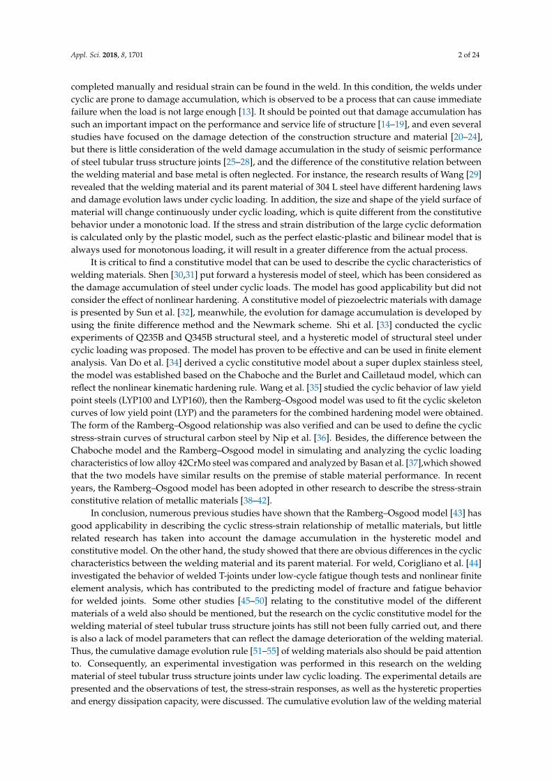
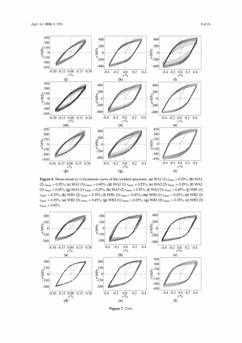
The cyclic stress-strain (σ-ε) curves of welded specimens and steel specimens are shown in Figures 6 and 7, respectively, in which the abscissa axis represents the strain of the specimen, and the ordinate axis represents the stress. It can be seen that the stress-strain constitutive relation of the materials reflected by the hysteretic curves changes with the increase of cyclic cycles under cyclic loading. As can be studied analytically, each of the semi-cycles contains two main stages, that is, the loading stage with curvilinear segment and the unloading stage with approximate liner segment, respectively. There is an apparent difference between the curves of welded materials and steels. The welded material shows obvious damage degradation, that is, the stress amplitudes increase slightly only at the beginning of the loading, then decrease gradually with the increase of cyclic cycles, which indicate that the cyclic softening behavior of the welding material is apparent as the imposed displacement cycles increase, on the contrary, the steel shows cyclic hardening characteristics. During the cycling process, the stress level of the welded materials is higher than that of the steel specimens under the same working condition, but the cycling life of the welded material is less than that of the steel. This indicates that the welded material was hardened to a certain extent due to the influence of complex factors such as the welding process with high temperature, but its ability of plastic

Microcrack appeared

Crackwidened

Figure 5. Damage process of welded specimen in low cycle fatigue test. (a) Crack appeared in specimen;(b) Crack develop; (c) Specimen fractured at the maximum main crack.

3.2. Cyclic Behavior and Damage Analysis

The number of semi-cycles until the specimens were fractured are listed in Table 3, which areabout the welding material and its base material of welded joints in the steel tubular truss structure.It can be revealed by Table 3 that the cyclic life of the welded metal is less than that of the base metalwith the same working condition, which indicates that the speed of damage accumulation of thewelding material is faster than that of the steel, in other words, the welding materials accumulatedamage more easily than the base materials. The cycling life of the welding materials decreases withthe increase of the loading strain amplitude. The higher the strain amplitude level, the faster thedegradation rate of the specimens under cyclic loading, and resulting in earlier destruction. Table 3also shows that the influence of the steel rolling direction on the cycling life of steel is mainly reflectedin Q235 steels.

Table 3. Number of half cycles of welding material and steel.

SpecimensWelded Specimens Steel Specimens

WA1 WA2 WA3 WB1 WB2 WB3 SA1 SA2 SB1 SB2

(1) (0.25%) 3091 3810 3430 4351 4205 4293 4321 3789 4766 4703(2) (0.35%) 1865 1801 1831 2223 1992 1973 2109 1983 2525 2607(3) (0.45%) 1089 994 977 1559 1165 1106 1301 976 1639

The cyclic stress-strain (σ-ε) curves of welded specimens and steel specimens are shown inFigures 6 and 7, respectively, in which the abscissa axis represents the strain of the specimen, and theordinate axis represents the stress. It can be seen that the stress-strain constitutive relation of thematerials reflected by the hysteretic curves changes with the increase of cyclic cycles under cyclicloading. As can be studied analytically, each of the semi-cycles contains two main stages, that is,the loading stage with curvilinear segment and the unloading stage with approximate liner segment,respectively. There is an apparent difference between the curves of welded materials and steels.The welded material shows obvious damage degradation, that is, the stress amplitudes increaseslightly only at the beginning of the loading, then decrease gradually with the increase of cycliccycles, which indicate that the cyclic softening behavior of the welding material is apparent as theimposed displacement cycles increase, on the contrary, the steel shows cyclic hardening characteristics.During the cycling process, the stress level of the welded materials is higher than that of the steelspecimens under the same working condition, but the cycling life of the welded material is lessthan that of the steel. This indicates that the welded material was hardened to a certain extent

Appl. Sci. 2018, 8, 1701 7 of 24

due to the influence of complex factors such as the welding process with high temperature, but itsability of plastic deformation has been weakened, which makes the welded material more prone todamage accumulation and damage degradation than its base metal. Furthermore, it is suggestedthat the constitutive relation between the welded metal and its base metal should be considereddistinguishingly and the damage accumulation should be considered in the cyclic nonlinear analysisof the direct welded joints of the tubular truss structures.

Figure 6 contains the hysteretic curves of the welding materials under different conditions ofweld seam types, base metal types, and loading strain amplitudes. It can be seen from the curvesthat in addition to the degradation of the cyclic stress amplitude, the hysteretic curve of the weldedmetal shows a gradual “down” trend with the increase of the cyclic cycles, that is, the damageaccumulation caused degradation of bearing capacity and unloading stiffness. Furthermore, the areaaround the hysteresis loop decreases with the increase of the cyclic cycles, which means that thedamage accumulation can also lead to a decrease in energy dissipation capacity. In a word, undercyclic loading, the damage of the welded metal was expanding and accumulating, which is themain reason for the performance degradation until the final failure. For the existing constitutivemodels of metallic materials, the damage degradation behavior of welded materials has been seldomconsidered and the failure mechanism of materials and structures due to damage accumulation cannotbe accurately revealed.


deformation has been weakened, which makes the welded material more prone to damage accumulation and damage degradation than its base metal. Furthermore, it is suggested that the constitutive relation between the welded metal and its base metal should be considered distinguishingly and the damage accumulation should be considered in the cyclic nonlinear analysis of the direct welded joints of the tubular truss structures.

Figure 6 contains the hysteretic curves of the welding materials under different conditions of weld seam types, base metal types, and loading strain amplitudes. It can be seen from the curves that in addition to the degradation of the cyclic stress amplitude, the hysteretic curve of the welded metal shows a gradual “down” trend with the increase of the cyclic cycles, that is, the damage accumulation caused degradation of bearing capacity and unloading stiffness. Furthermore, the area around the hysteresis loop decreases with the increase of the cyclic cycles, which means that the damage accumulation can also lead to a decrease in energy dissipation capacity. In a word, under cyclic loading, the damage of the welded metal was expanding and accumulating, which is the main reason for the performance degradation until the final failure. For the existing constitutive models of metallic materials, the damage degradation behavior of welded materials has been seldom considered and the failure mechanism of materials and structures due to damage accumulation cannot be accurately revealed.

(a) (b) (c)

(d) (e) (f)

(g) (h) (i)

-0.30 -0.15 0.00 0.15 0.30-400

-200

0

200

400

σ/M

Pa

ε/%-0.4 -0.2 0.0 0.2 0.4

-400

-200

0

200

400

σ/M

Pa

ε/%-0.4 -0.2 0.0 0.2 0.4

-400

-200

0

200

400

σ/M

Pa

ε/%

-0.30 -0.15 0.00 0.15 0.30-450-300-150

0150300450

σ/M

Pa

ε/%-0.4 -0.2 0.0 0.2 0.4

-400

-200

0

200

400

σ/M

Pa

ε/% -0.4 -0.2 0.0 0.2 0.4-400

-200

0

200

400

σ/M

Pa

ε/%

-0.30 -0.15 0.00 0.15 0.30-450-300-150

0150300450

σ/M

Pa

ε/%-0.4 -0.2 0.0 0.2 0.4

-400

-200

0

200

400

σ/M

Pa

ε/%-0.4 -0.2 0.0 0.2 0.4

-400

-200

0

200

400

σ/M

Pa

ε/%

Figure 6. Cont.

Appl. Sci. 2018, 8, 1701 8 of 24


(j) (k) (l)

(m) (n) (o)

(p) (q) (r)

Figure 6. Stress-strain (σ-ε) hysteresis curve of the welded specimen. (a) WA1 (1) εmax = 0.25%; (b) WA1 (2) εmax = 0.35%; (c) WA1 (3) εmax = 0.45%; (d) WA2 (1) εmax = 0.25%; (e) WA2 (2) εmax = 0.35%; (f) WA2 (3) εmax = 0.45%; (g) WA3 (1) εmax = 0.25%; (h) WA3 (2) εmax = 0.35%; (i) WA3 (3) εmax = 0.45%; (j) WB1 (1) εmax = 0.25%; (k) WB1 (2) εmax = 0.35%; (l) WB1 (3) εmax = 0.45%; (m) WB2 (1) εmax = 0.25%; (n) WB2 (2) εmax = 0.35%; (o) WB2 (3) εmax = 0.45%; (p) WB3 (1) εmax = 0.25%; (q) WB3 (2) εmax = 0.35%; (r) WB3 (3) εmax = 0.45%.

(a) (b) (c)

(d) (e) (f)

-0.30 -0.15 0.00 0.15 0.30-450-300-150

0150300450

σ/M

Pa

ε/%-0.4 -0.2 0.0 0.2 0.4

-400

-200

0

200

400

σ/M

Pa

ε/%-0.4 -0.2 0.0 0.2 0.4

-400

-200

0

200

400

σ/M

Pa

ε/%

-0.30 -0.15 0.00 0.15 0.30-450-300-150

0150300450

σ/M

Pa

ε/%-0.4 -0.2 0.0 0.2 0.4

-400

-200

0

200

400

σ/M

Pa

ε/%-0.4 -0.2 0.0 0.2 0.4

-400

-200

0

200

400

σ/M

Pa

ε/%

-0.30 -0.15 0.00 0.15 0.30-450-300-150

0150300450

σ/M

Pa

ε/%-0.4 -0.2 0.0 0.2 0.4

-400

-200

0

200

400

σ/M

Pa

ε/%-0.4 -0.2 0.0 0.2 0.4

-450-300-150

0150300450

σ/M

Pa

ε/%

-0.30 -0.15 0.00 0.15 0.30

-300-150

0150300

σ/M

Pa

ε/%-0.4 -0.2 0.0 0.2 0.4

-300-150

0150300

σ/M

Pa

ε/%-0.4 -0.2 0.0 0.2 0.4

-400

-200

0

200

400

σ/M

Pa

ε/%

-0.30 -0.15 0.00 0.15 0.30

-300-150

0150300

σ/M

Pa

ε/% -0.4 -0.2 0.0 0.2 0.4

-300-150

0150300

σ/M

Pa

ε/%-0.4 -0.2 0.0 0.2 0.4

-450-300-150

0150300450

σ/M

Pa

ε/%

Figure 6. Stress-strain (σ-ε) hysteresis curve of the welded specimen. (a) WA1 (1) εmax = 0.25%; (b) WA1(2) εmax = 0.35%; (c) WA1 (3) εmax = 0.45%; (d) WA2 (1) εmax = 0.25%; (e) WA2 (2) εmax = 0.35%; (f) WA2(3) εmax = 0.45%; (g) WA3 (1) εmax = 0.25%; (h) WA3 (2) εmax = 0.35%; (i) WA3 (3) εmax = 0.45%; (j) WB1 (1)εmax = 0.25%; (k) WB1 (2) εmax = 0.35%; (l) WB1 (3) εmax = 0.45%; (m) WB2 (1) εmax = 0.25%; (n) WB2 (2)εmax = 0.35%; (o) WB2 (3) εmax = 0.45%; (p) WB3 (1) εmax = 0.25%; (q) WB3 (2) εmax = 0.35%; (r) WB3 (3)εmax = 0.45%.


(j) (k) (l)

(m) (n) (o)

(p) (q) (r)

Figure 6. Stress-strain (σ-ε) hysteresis curve of the welded specimen. (a) WA1 (1) εmax = 0.25%; (b) WA1 (2) εmax = 0.35%; (c) WA1 (3) εmax = 0.45%; (d) WA2 (1) εmax = 0.25%; (e) WA2 (2) εmax = 0.35%; (f) WA2 (3) εmax = 0.45%; (g) WA3 (1) εmax = 0.25%; (h) WA3 (2) εmax = 0.35%; (i) WA3 (3) εmax = 0.45%; (j) WB1 (1) εmax = 0.25%; (k) WB1 (2) εmax = 0.35%; (l) WB1 (3) εmax = 0.45%; (m) WB2 (1) εmax = 0.25%; (n) WB2 (2) εmax = 0.35%; (o) WB2 (3) εmax = 0.45%; (p) WB3 (1) εmax = 0.25%; (q) WB3 (2) εmax = 0.35%; (r) WB3 (3) εmax = 0.45%.

(a) (b) (c)

(d) (e) (f)

-0.30 -0.15 0.00 0.15 0.30-450-300-150

0150300450

σ/M

Pa

ε/%-0.4 -0.2 0.0 0.2 0.4

-400

-200

0

200

400

σ/M

Pa

ε/%-0.4 -0.2 0.0 0.2 0.4

-400

-200

0

200

400

σ/M

Pa

ε/%

-0.30 -0.15 0.00 0.15 0.30-450-300-150

0150300450

σ/M

Pa

ε/%-0.4 -0.2 0.0 0.2 0.4

-400

-200

0

200

400

σ/M

Pa

ε/%-0.4 -0.2 0.0 0.2 0.4

-400

-200

0

200

400

σ/M

Pa

ε/%

-0.30 -0.15 0.00 0.15 0.30-450-300-150

0150300450

σ/M

Pa

ε/%-0.4 -0.2 0.0 0.2 0.4

-400

-200

0

200

400

σ/M

Pa

ε/%-0.4 -0.2 0.0 0.2 0.4

-450-300-150

0150300450

σ/M

Pa

ε/%

-0.30 -0.15 0.00 0.15 0.30

-300-150

0150300

σ/M

Pa

ε/%-0.4 -0.2 0.0 0.2 0.4

-300-150

0150300

σ/M

Pa

ε/%-0.4 -0.2 0.0 0.2 0.4

-400

-200

0

200

400

σ/M

Pa

ε/%

-0.30 -0.15 0.00 0.15 0.30

-300-150

0150300

σ/M

Pa

ε/% -0.4 -0.2 0.0 0.2 0.4

-300-150

0150300

σ/M

Pa

ε/%-0.4 -0.2 0.0 0.2 0.4

-450-300-150

0150300450

σ/M

Pa

ε/%

Figure 7. Cont.

Appl. Sci. 2018, 8, 1701 9 of 24


(g) (h) (i)

(j) (k)

Figure 7. Stress-strain (σ-ε) hysteresis curve of the steel (base metal) specimen.(a) SA1 (1) εmax = 0.25%; (b) SA1 (2) εmax = 0.35%; (c) SA1 (3) εmax = 0.45%; (d) SA2 (1) εmax = 0.25%; (e) SA2 (2) εmax = 0.35%; (f) SA2 (3) εmax = 0.45%; (g) SB1 (1) εmax = 0.25%; (h) SB1 (2) εmax = 0.35%; (i) SB2 (1) εmax = 0.25%; (j) SB2 (2) εmax = 0.35%; (k) SB2 (3) εmax = 0.45%.

3.3. Variation of Cyclic Stress Amplitude

As seen in Figure 8, obtained through Figures 6 and 7 are curves about the variation of the cyclic stress amplitudes with increases to the cyclic cycles of the welding materials and steels, in which the non-dimensional parameter η was obtained from the numbers of semi-cycles in a certain time divided by the numbers of semi-cycles at the end of the test. Each picture in Figure 8 contains three stress amplitude-η curves that were obtained from three loading conditions with different strain amplitudes, which can be realized from Table 1 and Figure 4. Therefore, the influence of weld form, base material type, and loading mode on the damage accumulation of the welding materials will be compared and analyzed.

As shown in Figure 8a–f, the degradation of the cyclic stress amplitude is basically divided into three stages, corresponding to the three stages of crack development in a low-cycle fatigue test. The stress amplitude degenerated rapidly in the first stage, which has a number of cycles less than 20%, corresponding to the initial stage of fatigue crack development. When the numbers of cycle reached about 20%, the stress amplitude decreased steadily, and corresponded to the stable stage of fatigue crack development, which is the longest stage of stress amplitude degradation. Finally, the stress amplitude degenerated sharply and the specimens were fractured rapidly when the number of cycles reached about 80% or 90%. Loading strain amplitude has a certain effect on the damage degradation rate. As we can see, there are three curves in each picture of Figure 8a–f, and the loading train amplitude of the curves increased in turn. It indicates that the cyclic stress amplitude increased with the increasing of the controlled strain amplitude. Moreover, the specimens with larger controlled strain amplitude degenerated faster in the failure stage. All of the above indicate that the larger the controlled loading strain amplitude, the faster the rate of damage accumulation.

The influence of type of specimens also should be discussed. As shown in Figure 8g–h, the stress amplitude-η curves of WA and WB welding specimens are compared at the same time. It can be concluded that the stress amplitude of the welding materials with Q235 base metal degenerated faster than that of the Q345 base metal, and the curves of WB specimens are more concentrated than those of WA specimens, indicating that the influence of the loading strain amplitude in the rate of damage accumulation is more significant for welding materials with a Q235 base steel. For the influence of the welding mode, the welded form of No. (1) specimens with the Q235 and Q345 base metal is a butt

-0.30 -0.15 0.00 0.15 0.30-450-300-150

0150300450

σ/M

Pa

ε/%-0.4 -0.2 0.0 0.2 0.4

-450-300-150

0150300450

σ/M

Pa

ε/%-0.30 -0.15 0.00 0.15 0.30-450

-300-150

0150300450

σ/M

Pa

ε/%

-0.4 -0.2 0.0 0.2 0.4-450-300-150

0150300450

σ/M

Pa

ε/%-0.4 -0.2 0.0 0.2 0.4

-450-300-150

0150300450

σ/M

Pa

ε/%

Figure 7. Stress-strain (σ-ε) hysteresis curve of the steel (base metal) specimen.(a) SA1 (1) εmax = 0.25%;(b) SA1 (2) εmax = 0.35%; (c) SA1 (3) εmax = 0.45%; (d) SA2 (1) εmax = 0.25%; (e) SA2 (2) εmax = 0.35%;(f) SA2 (3) εmax = 0.45%; (g) SB1 (1) εmax = 0.25%; (h) SB1 (2) εmax = 0.35%; (i) SB2 (1) εmax = 0.25%;(j) SB2 (2) εmax = 0.35%; (k) SB2 (3) εmax = 0.45%.

3.3. Variation of Cyclic Stress Amplitude

As seen in Figure 8, obtained through Figures 6 and 7 are curves about the variation of the cyclicstress amplitudes with increases to the cyclic cycles of the welding materials and steels, in which thenon-dimensional parameter η was obtained from the numbers of semi-cycles in a certain time divided bythe numbers of semi-cycles at the end of the test. Each picture in Figure 8 contains three stress amplitude-ηcurves that were obtained from three loading conditions with different strain amplitudes, which can berealized from Table 1 and Figure 4. Therefore, the influence of weld form, base material type, and loadingmode on the damage accumulation of the welding materials will be compared and analyzed.

As shown in Figure 8a–f, the degradation of the cyclic stress amplitude is basically dividedinto three stages, corresponding to the three stages of crack development in a low-cycle fatigue test.The stress amplitude degenerated rapidly in the first stage, which has a number of cycles less than 20%,corresponding to the initial stage of fatigue crack development. When the numbers of cycle reachedabout 20%, the stress amplitude decreased steadily, and corresponded to the stable stage of fatiguecrack development, which is the longest stage of stress amplitude degradation. Finally, the stressamplitude degenerated sharply and the specimens were fractured rapidly when the number of cyclesreached about 80% or 90%. Loading strain amplitude has a certain effect on the damage degradationrate. As we can see, there are three curves in each picture of Figure 8a–f, and the loading trainamplitude of the curves increased in turn. It indicates that the cyclic stress amplitude increased withthe increasing of the controlled strain amplitude. Moreover, the specimens with larger controlledstrain amplitude degenerated faster in the failure stage. All of the above indicate that the larger thecontrolled loading strain amplitude, the faster the rate of damage accumulation.

The influence of type of specimens also should be discussed. As shown in Figure 8g–h, the stressamplitude-η curves of WA and WB welding specimens are compared at the same time. It can beconcluded that the stress amplitude of the welding materials with Q235 base metal degenerated fasterthan that of the Q345 base metal, and the curves of WB specimens are more concentrated than thoseof WA specimens, indicating that the influence of the loading strain amplitude in the rate of damageaccumulation is more significant for welding materials with a Q235 base steel. For the influence of thewelding mode, the welded form of No. (1) specimens with the Q235 and Q345 base metal is a butt

Appl. Sci. 2018, 8, 1701 10 of 24

weld (the dotted line in Figure 8g–h), whose stress amplitudes are lower than that of the fillet weldspecimens under the same working conditions. This can be attributed to the fact that the structure andwelding process of the fillet welds are more complex than the butt welds, resulting in more damageaccumulation than the fillet welds.


weld (the dotted line in Figure 8g–h), whose stress amplitudes are lower than that of the fillet weld specimens under the same working conditions. This can be attributed to the fact that the structure and welding process of the fillet welds are more complex than the butt welds, resulting in more damage accumulation than the fillet welds.

(a) (b) (c)

(d) (e) (f)

(g) (h)

(i) (j)

Figure 8. Stress amplitude-dimensionless (σm-η) half cycle of welding material and steel. (a) WA1; (b) WA2; (c) WA3; (d) WB1; (e) WB2; (f) WB3; (g) WA; (h) WB; (i) SA1; (j) SB2.

3.4. EnergyDissipation Behavior

Referring to the consideration of energy dissipation in the Park-Ang damage cumulative model [58], the cumulative energy dissipation is dealt with in the dimensionless method, and the energy dissipation capacity is reflected by the cumulative energy dissipation coefficient ξa. The expression is shown in Equation (1) [58]. Eu is the ultimate hysteretic energy under monotonic loading, which can be calculated from the area enclosed by the stress-strain curves of monotonic tensile test and the coordinate axis. Ei is the actual dissipated energy of the No. i semi-cycle, which can be calculated from the area enclosed by the cyclic stress-strain hysteretic curves of cyclic loading test and the

0.0 0.2 0.4 0.6 0.8 1.0150200250300350400450

σ m/MPa WA1(1) WA1(2) WA1(3)η 0.0 0.2 0.4 0.6 0.8 1.0200250300350400450

σ m/MPa WA2(1) WA2(2) WA2(3)

η0.0 0.2 0.4 0.6 0.8 1.0200250300350400450

σ m/MPa

η

WA3(1) WA3(2) WA3(3)

0.0 0.2 0.4 0.6 0.8 1.0200250300350400450

σ m/MPa

η

WB1(1) WB1(2) WB1(3)

0.0 0.2 0.4 0.6 0.8 1.0200250300350400450σ m/MPa

η

WB2(1) WB2(2) WB2(3) 0.0 0.2 0.4 0.6 0.8 1.0200250300350400450

σ m/MPa WB3(1) WB3(2) WB3(3)η

0.0 0.2 0.4 0.6 0.8 1.0200250300350400

σ m/MPa

η

SA1(1) SA1(2) SA1(3) 0.0 0.2 0.4 0.6 0.8 1.0200250300350400450500550

η

σ m/MPa SB2(1) SB2(2) SB2(3)

0.0 0.2 0.4 0.6 0.8 1.0 1.2 1.4200250300350400450

σ m/MPa

η

WA1(1) WA2(1) WA3(1) WA1(2) WA2(2) WA3(2) WA1(3) WA2(3) WA3(3) 0.0 0.2 0.4 0.6 0.8 1.0 1.2 1.4 1.6200250300350400450

σ m/MPa

η

WB1(1) WB1(2) WB1(3) WB2(1) WB2(2) WB2(3) WB3(1) WB3(2) WB3(3)Figure 8. Stress amplitude-dimensionless (σm-η) half cycle of welding material and steel. (a) WA1;(b) WA2; (c) WA3; (d) WB1; (e) WB2; (f) WB3; (g) WA; (h) WB; (i) SA1; (j) SB2.

3.4. EnergyDissipation Behavior

Referring to the consideration of energy dissipation in the Park-Ang damage cumulativemodel [58], the cumulative energy dissipation is dealt with in the dimensionless method, and the energydissipation capacity is reflected by the cumulative energy dissipation coefficient ξa. The expressionis shown in Equation (1) [58]. Eu is the ultimate hysteretic energy under monotonic loading, whichcan be calculated from the area enclosed by the stress-strain curves of monotonic tensile test and thecoordinate axis. Ei is the actual dissipated energy of the No. i semi-cycle, which can be calculated

Appl. Sci. 2018, 8, 1701 11 of 24

from the area enclosed by the cyclic stress-strain hysteretic curves of cyclic loading test and thecoordinate axis. Then, ξa-η curve of welded material is depicted in Figure 9, it can be seen that theslope of the curves decreases with the increase of cyclic cycles, which means that the rate of cumulativeenergy dissipation decreases gradually, in other words, the enclosing area of the hysteretic loopsdecreases with the increase of cyclic cycles, and the energy dissipation capacity decreases gradually.It is due to the continuous damage accumulation of the welding materials under cyclic loading. In aword, the cumulative damage rule of the welding material can be discussed through cumulativeenergy dissipation behavior is consistent with the law of stress amplitude degradation. That is, withthe continuous development of damage accumulation under cyclic loading, the amplitude of cyclicstress, unloading stiffness, and energy dissipation capacity of the welded metal, these degenerategradually until failure occurs, and compared with the base metal, the welded metal is more prone todamage accumulation.

ξa =

n∑

i=1Ei

Eu(1)


coordinate axis. Then, ξa-η curve of welded material is depicted in Figure 9, it can be seen that the slope of the curves decreases with the increase of cyclic cycles, which means that the rate of cumulative energy dissipation decreases gradually, in other words, the enclosing area of the hysteretic loops decreases with the increase of cyclic cycles, and the energy dissipation capacity decreases gradually. It is due to the continuous damage accumulation of the welding materials under cyclic loading. In a word, the cumulative damage rule of the welding material can be discussed through cumulative energy dissipation behavior is consistent with the law of stress amplitude degradation. That is, with the continuous development of damage accumulation under cyclic loading, the amplitude of cyclic stress, unloading stiffness, and energy dissipation capacity of the welded metal, these degenerate gradually until failure occurs, and compared with the base metal, the welded metal is more prone to damage accumulation.

u

n

ii

a E

E== 1ξ (1)

(a) (b) (c)

(d) (e) (f)

Figure 9. ξa-η curve of welding material. (a) WA1ξa-η; (b) WA2ξa-η; (c) WA3ξa-η; (d) WB1ξa-η; (e) WA2ξa-η; (f) WA3ξa-η.

4. An Evolution Equation of Damage Accumulation for Welding Materials

Damage variable D is used to represent the damage degree of material in damage theory [59]. Meanwhile, the experimental results show that the macroscopic mechanical behavior of the damage of the welding material can be expressed in both energy and deformation. Therefore, in order to describe the microscopic structural damage mechanism of the material in macroscopic mechanics, the evolution equation of the damage variable D of the welding material under cyclic loading is established based on the experimental results. As shown in Equation (2), the Park-Ang [58] model is suitable for structural damage cumulative analysis, in which δm and δu is the maximum deformation

with loading and ultimate deformation of material respectively, dE is the cumulative dissipation

of plastic energy, Fyδu is equivalent to the ultimate hysteretic energy under the monotonic load of perfect elastic-plastic condition.

0.2 0.4 0.6 0.8 1.00

10

20

30

40

WA1(1) WA1(2) WA1(3)

aξ

η 0.2 0.4 0.6 0.8 1.00

10

20

30

40

WA2(1) WA2(2) WA2(3)

aξ

η 0.2 0.4 0.6 0.8 1.00

10

20

30

40

WA3(1) WA3(2) WA3(3)

aξ

η

0.2 0.4 0.6 0.8 1.001020304050

η

WB1(1) WB1(2) WB1(3)

aξ

0.2 0.4 0.6 0.8 1.001020304050

η

aξ

WB2(1) WB2(2) WB2(3)

0.2 0.4 0.6 0.8 1.00

10

20

30

40

50

η

aξ

WB3(1) WB3(2) WB3(3)

Figure 9. ξa-η curve of welding material. (a) WA1ξa-η; (b) WA2ξa-η; (c) WA3ξa-η; (d) WB1ξa-η;(e) WA2ξa-η; (f) WA3ξa-η.

4. An Evolution Equation of Damage Accumulation for Welding Materials

Damage variable D is used to represent the damage degree of material in damage theory [59].Meanwhile, the experimental results show that the macroscopic mechanical behavior of the damageof the welding material can be expressed in both energy and deformation. Therefore, in order todescribe the microscopic structural damage mechanism of the material in macroscopic mechanics,the evolution equation of the damage variable D of the welding material under cyclic loading isestablished based on the experimental results. As shown in Equation (2), the Park-Ang [58] model issuitable for structural damage cumulative analysis, in which δm and δu is the maximum deformationwith loading and ultimate deformation of material respectively,

∫dE is the cumulative dissipation of

plastic energy, Fyδu is equivalent to the ultimate hysteretic energy under the monotonic load of perfectelastic-plastic condition.

Based on the above model, an evolution equation of damage variable D (2) for calculating thecumulative damage of the welding material is established, as seen in Equation (3), in which the effects

Appl. Sci. 2018, 8, 1701 12 of 24

of plastic strain and cumulative plastic energy dissipation on the damage accumulation of the weldingmaterial are considered comprehensively. In Equation (3), ε

pm is the maximum plastic strain in cyclic

process, εpu is the ultimate plastic strain of materials that can be obtained from the uniaxial tensile

test, Ei is the plastic deformation energy dissipation of No. i semi-cycles, which is equal to the area ofthe hysteresis loop in numerical value, Eu is the ultimate hysteretic energy under monotonic loading,which can be calculated from the area enclosed by the stress-strain curves of the monotonic tensile testand the coordinate axis, λ is a parameter means the weight of cumulative plastic energy dissipation,which can be calculated by the cyclic loading test results. Compared with Equation (2), the energy partof the model in Equation (3) is no longer confined to the perfect elastic-plastic condition, and the factthat the value of damage variable D is always less than or equal to 1 until fractured is ensured.

D =δm

δu+ β

∫dE

Fyδu(2)

D = (1− λ)εp

m

εpu

+n

∑i=n1

λEiEu

(3)

5. A Hysteresis Model with Damage Accumulation of Welding Materials

5.1. Basic Requirements of the Model

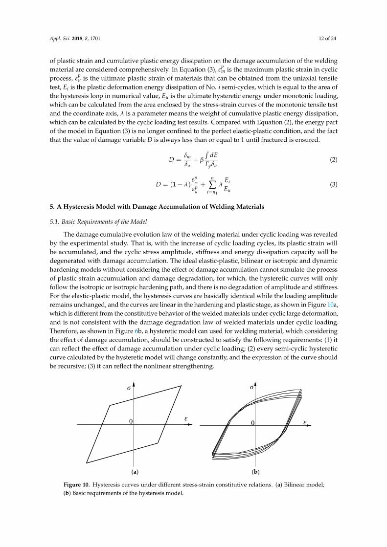
The damage cumulative evolution law of the welding material under cyclic loading was revealedby the experimental study. That is, with the increase of cyclic loading cycles, its plastic strain willbe accumulated, and the cyclic stress amplitude, stiffness and energy dissipation capacity will bedegenerated with damage accumulation. The ideal elastic-plastic, bilinear or isotropic and dynamichardening models without considering the effect of damage accumulation cannot simulate the processof plastic strain accumulation and damage degradation, for which, the hysteretic curves will onlyfollow the isotropic or isotropic hardening path, and there is no degradation of amplitude and stiffness.For the elastic-plastic model, the hysteresis curves are basically identical while the loading amplituderemains unchanged, and the curves are linear in the hardening and plastic stage, as shown in Figure 10a,which is different from the constitutive behavior of the welded materials under cyclic large deformation,and is not consistent with the damage degradation law of welded materials under cyclic loading.Therefore, as shown in Figure 6b, a hysteretic model can used for welding material, which consideringthe effect of damage accumulation, should be constructed to satisfy the following requirements: (1) itcan reflect the effect of damage accumulation under cyclic loading; (2) every semi-cyclic hystereticcurve calculated by the hysteretic model will change constantly, and the expression of the curve shouldbe recursive; (3) it can reflect the nonlinear strengthening.


(a) (b)

Figure 10. Hysteresis curves under different stress-strain constitutive relations. (a) Bilinear model; (b) Basic requirements of the hysteresis model.

5.2. Initial Loading Curve

The expression of the initial loading curve is shown in Equation (4), which is established though the uniaxial tensile test for a welded material and the curve is depicted in Figure 11a, in which the stages named I, II, and III correspond to the formulas in Equation (4), respectively. The constitutive equation contains the effect of damage, and the parameters will be fitted by the uniaxial tensile test results obtained before the cyclic test. Figure 11b is the fitting result of the WA1 specimen. And the results of the other specimens are shown in Table 4.

>+−

−−=

≤<=

≤=

20

0

21

1

;)()](1[

;;

ym

CC

yyy

y

bKD

E

εεεεε

εεσ

εεεσσεεεσ

(4)

Table 4. Parameter values of initial loading curve.

Base Metal

Welding Material E/Gpa σy/MPa K/Gpa m εy1/% εy2(ε0)/% εc/% b DC/%

Q235 Butt weld 239.70 391.70 2.73 0.77 0.16 1.50 21.25 0.065 59.24 Fillet weld 223.30 401.94 1.82 0.54 0.18 1.50 21.34 0.046 50.03


(a) (b)

Figure 11. Fitting results of the initial loading curve. (a) The schematic diagram of the initial loading curve; (b) Fitting result of the WA1 specimen.

ε

σ

0

σ

ε

0

ⅢⅡⅠ

εμ εc(ε0)εy2εy1

σyσμ

ε

σ

0.05 0.10 0.15 0.20 0.250100200300400500

σ/MPa

ε

Formula fitting Tset

Figure 10. Hysteresis curves under different stress-strain constitutive relations. (a) Bilinear model;(b) Basic requirements of the hysteresis model.

Appl. Sci. 2018, 8, 1701 13 of 24


The expression of the initial loading curve is shown in Equation (4), which is established thoughthe uniaxial tensile test for a welded material and the curve is depicted in Figure 11a, in which thestages named I, II, and III correspond to the formulas in Equation (4), respectively. The constitutiveequation contains the effect of damage, and the parameters will be fitted by the uniaxial tensile testresults obtained before the cyclic test. Figure 11b is the fitting result of the WA1 specimen. And theresults of the other specimens are shown in Table 4.

σ = Eε ; ε ≤ εy1

σ = σy ; εy1 < ε ≤ εy2

σ = [1− (DCε−ε0

εC−ε0)]K(ε + b)m ; ε > εy2

(4)


Base Metal Welding Material E/Gpa σy/MPa K/Gpa m εy1/% εy2(ε0)/% εc/% b DC/%

Q235Butt weld 239.70 391.70 2.73 0.77 0.16 1.50 21.25 0.065 59.24Fillet weld 223.30 401.94 1.82 0.54 0.18 1.50 21.34 0.046 50.03

Q345Butt weld 247.71 420.07 2.52 0.65 0.17 1.70 17.71 0.052 57.64Fillet weld 241.07 433.92 2.17 0.60 0.18 1.70 16.97 0.044 53.11


(a) (b)

Figure 10. Hysteresis curves under different stress-strain constitutive relations. (a) Bilinear model; (b) Basic requirements of the hysteresis model.


The expression of the initial loading curve is shown in Equation (4), which is established though the uniaxial tensile test for a welded material and the curve is depicted in Figure 11a, in which the stages named I, II, and III correspond to the formulas in Equation (4), respectively. The constitutive equation contains the effect of damage, and the parameters will be fitted by the uniaxial tensile test results obtained before the cyclic test. Figure 11b is the fitting result of the WA1 specimen. And the results of the other specimens are shown in Table 4.

>+−

−−=

≤<=

≤=

20

0

21

1

;)()](1[

;;

ym

CC

yyy

y

bKD

E

εεεεε

εεσ

εεεσσεεεσ

(4)


Base Metal

Welding Material E/Gpa σy/MPa K/Gpa m εy1/% εy2(ε0)/% εc/% b DC/%



(a) (b)

Figure 11. Fitting results of the initial loading curve. (a) The schematic diagram of the initial loading curve; (b) Fitting result of the WA1 specimen.

ε

σ

0

σ

ε

0

ⅢⅡⅠ

εμ εc(ε0)εy2εy1

σyσμ

ε

σ

0.05 0.10 0.15 0.20 0.250100200300400500σ/MPa

ε

Formula fitting TsetFigure 11. Fitting results of the initial loading curve. (a) The schematic diagram of the initial loadingcurve; (b) Fitting result of the WA1 specimen.

5.3. Cyclic Stress-Strain Curve Based on Ramberg–Osgood Model

The stress-strain hysteretic curves obtained from different loading strain amplitudes are placed inthe same coordinate system, and the maximum and minimum stress peaks are connected to obtain thecyclic stress-strain curves, just as depicted in Figure 12, which does not represent the true stress-strainpath of the welded material under cyclic loading, but is a cyclic stress-strain curve under steady state.Researches [33,60,61] show that the cyclic stress-strain curves of steady-state are different from thoseunder monotonic loading, the cyclic stress-strain curve can be described by the Ramberg–Osgood [43]model approximately, as presented in Equation (5). E0 and K0 are the initial elastic modulus andhardening coefficients, respectively, which can be fitted by the Low-cycle fatigue test of the weldingmaterials. The parameters of Equation (5) are summarized in Table 5.

ε =

σE0

+(

σK0

)n0; σ > 0

σE0−(−σK0

)n0; σ ≤ 0

(5)

Appl. Sci. 2018, 8, 1701 14 of 24

Got the logarithm of Equation (5), just as Equation (6), then, let y = ln(ε − σE0) , x = ln σ,

b = −n0 ln K0, Equation (6) will transform to Equation (7), thus, linear fitting can be performed.

ln(ε− σ

E0) = n0(ln σ− ln K0) (6)

y = n0x + b (7)


5.3. Cyclic Stress-Strain Curve Based on Ramberg–Osgood Model

The stress-strain hysteretic curves obtained from different loading strain amplitudes are placed in the same coordinate system, and the maximum and minimum stress peaks are connected to obtain the cyclic stress-strain curves, just as depicted in Figure 12, which does not represent the true stress-strain path of the welded material under cyclic loading, but is a cyclic stress-strain curve under steady state. Researches [33,60,61] show that the cyclic stress-strain curves of steady-state are different from those under monotonic loading, the cyclic stress-strain curve can be described by the Ramberg–Osgood [43] model approximately, as presented in Equation (5). E0 and K0 are the initial elastic modulus and hardening coefficients, respectively, which can be fitted by the Low-cycle fatigue test of the welding materials. The parameters of Equation (5) are summarized in Table 5.

≤

−−

>

+

=

0;

0;

0

0

00

00

σσσ

σσσ

εn

n

KE

KE (5)

Got the logarithm of Equation (5), just as Equation (6), then, let )ln(0E

y σε −= , σln=x ,

00 ln Knb −= , Equation (6) will transform to Equation (7), thus, linear fitting can be performed.

)ln(ln)ln( 000

KnE

−=− σσε (6)

bxny += 0(7)

Figure 12. Schematic diagram of cyclic stress-strain curve.

Table 5. Parameters of the cyclic stress-strain curves for welding materials.

With Q235 Base Metal With Q345 Base Metal Specimens E0/GPa K0/MPa n0 Specimens E0/GPa K0/MPa n0

WA1 239.700 1266 4.784 WB1 247.710 953 8.099 WA2 223.000 1331 5.531 WB2 241.070 939 8.610 WA3 223.000 1466 6.203 WB3 241.070 885 9.272

5.4. A Model of Hysteretic Curve with Damage Accumulation

The Ramberg–Osgood model has proven to be a good description of the cyclic stress-strain relationship of the metallic materials by many studies, and the Masing criterion shows that the stress-strain path under cyclic loading can be described by amplifying 1 time the cyclic stress-strain curve

cyclic stress-strain curveσ

ε

Figure 12. Schematic diagram of cyclic stress-strain curve.

Table 5. Parameters of the cyclic stress-strain curves for welding materials.

With Q235 Base Metal With Q345 Base Metal

Specimens E0/GPa K0/MPa n0 Specimens E0/GPa K0/MPa n0

WA1 239.700 1266 4.784 WB1 247.710 953 8.099WA2 223.000 1331 5.531 WB2 241.070 939 8.610WA3 223.000 1466 6.203 WB3 241.070 885 9.272

5.4. A Model of Hysteretic Curve with Damage Accumulation

The Ramberg–Osgood model has proven to be a good description of the cyclic stress-strainrelationship of the metallic materials by many studies, and the Masing criterion shows that thestress-strain path under cyclic loading can be described by amplifying 1 time the cyclic stress-straincurve in a steady state [62–65], such as explained in Figure 13. Based on the theory, and consideringthe effect of the damage, the evolution equation of damage variable D is introduced to construct amodel of the hysteretic curve for the welding material. As shown in Figure 14, a hysteresis model withdamage accumulation of welding materials is presented, in which the No. n semi-cycle is shown as anexample to describe the hysteresis criterion.


in a steady state [62–65], such as explained in Figure 13. Based on the theory, and considering the effect of the damage, the evolution equation of damage variable Dis introduced to construct a model of the hysteretic curve for the welding material. As shown in Figure 14, a hysteresis model with damage accumulation of welding materials is presented, in which the No. n semi-cycle is shown as an example to describe the hysteresis criterion.

Figure 13. Masing behavior.

Curve An-Cn-Bn is the loading curve of No. n semi-cycle, which is constructed by considering nonlinear loading. Point An is the starting point of then semi-cycle loading curve, and Bn is the final point of the loading curve, but is the starting point of the n semi-cycle unloading curve. )(nD

mσ is the stress amplitude of the No. n semi-cyclic stress-strain curve and the ordinate of point Bn. The stress amplitude of each semi-cycle will be degraded with damage accumulating, so )(nD

mσ is thought of as the damage stress amplitude, which can be calculated by Equation (8) based on damage mechanics theory, mσ is the initial stress amplitude, nD is the cumulative damage variable after nth semi-cycle, which can be calculated by Equation (3),η and ξ are the damage parameters that can be fitted by the low-cycle fatigue test results of the welding material. Curve Bn-An+1 is the unloading curve of No. n semi-cycle, and the unloading process is approximately elastic. D

nE is the elastic modulus

with damage accumulation, which in respect of nD can be calculated by Equation (9) based on

damage mechanics theory and Shen [30,31]. 0E is the original elastic modulus, g and h are the damage parameters like η and ξ.

mnnD

m D σξησ )()( −= (8)

0)( EhDgE nDn −= (9)

AB

C

FED0 ε

σ

cyclic σ-ε curve

Figure 13. Masing behavior.

Appl. Sci. 2018, 8, 1701 15 of 24

Curve An-Cn-Bn is the loading curve of No. n semi-cycle, which is constructed by considering nonlinearloading. Point An is the starting point of the n semi-cycle loading curve, and Bn is the final point of theloading curve, but is the starting point of the n semi-cycle unloading curve. σ

D(n)m is the stress amplitude

of the No. n semi-cyclic stress-strain curve and the ordinate of point Bn. The stress amplitude of eachsemi-cycle will be degraded with damage accumulating, so σ

D(n)m is thought of as the damage stress

amplitude, which can be calculated by Equation (8) based on damage mechanics theory, σm is the initialstress amplitude, Dn is the cumulative damage variable after nth semi-cycle, which can be calculated byEquation (3),η and ξ are the damage parameters that can be fitted by the low-cycle fatigue test results of thewelding material. Curve Bn-An+1 is the unloading curve of No. n semi-cycle, and the unloading process isapproximately elastic. ED

n is the elastic modulus with damage accumulation, which in respect of Dn can becalculated by Equation (9) based on damage mechanics theory and Shen [30,31]. E0 is the original elasticmodulus, g and h are the damage parameters like η and ξ.

σD(n)m = (η − ξ Dn)σm (8)

EDn = (g− hDn)E0 (9)Appl. Sci. 2018, 8, x FOR PEER REVIEW 16 of 25

Figure 14. Hysteretic model of welding material considering cumulative damage under cyclic loading.

Overall, the hysteresis model considering damage accumulation of welding material is depicted in Figure 14, the expressions of the model are as follows:

(1) unloading curve (Linear)

nnDnn tE += εσ (10)

)( )(B

Dn

nDmn Et εσ −= (11)

In Equations (10) and (11), σn and εn are stress and strain values of point at nth semi-cycle curves, tn is the parameter for determining the shape of the curve, εB is the strain amplitude.

(2) loading curve (nonlinear)

The expression of the model is established based on the damage degenerating law, Ramberg–Osgood model and Masing behavior.

−+

′−−−

−+

′

−+−

=′

′

0)(;

0(;

)()()(

)()()(

＜

）＞

nDmnB

n

nnD

mDn

nDmn

nDmnB

nnDmn

Dn

nDmn

n

KE

KE

σσεσσσσ

σσεσσσσ

ε (12)

(12) In Equation (13), )(nD

mσ and DnE are degenerated according to Formulas (10) and (11), K’ and n’

can be fitted by the data of the low-cycle fatigue test. Equation (13) shows that, considering the effect of damage accumulation, the stress-strain paths of each semi-cycle determined by the model do not coincide completely even in the case of constant amplitude cycling. And the unloading stiffness, bearing capacity, and energy dissipation capacity are irreversibly degraded with the increase of the number of half cycles, which is consistent with the damage accumulation law of the welding materials reflected in the test.

In conclusion, the hysteresis model with damage accumulation for welding materials is as follows:

unloading curveloading curve

(n+1)th semi-cycle

unloading curve

•

••

•

••

••

σy

Yn(ε(n)y ,σ（n)

y )

EDn+1

σD(n+1)m

Cn+1(εCn+1,σCn+1)

Cn(εCn ,σCn)(n+2)th semi-cycle

nth semi-cycle

εpn+1

cyclic σ-ε curve

An(εAn ,σAn) An+2(εAn+2 ,σAn+2)

σD(n)m

ε

σ

EDn

loading curveE0

An+1(εAn+1,σAn+1)

Bn+1(εB ,σD(n+1)m )

Bn(εB ,σD(n)m )

0•

Figure 14. Hysteretic model of welding material considering cumulative damage under cyclic loading.

Overall, the hysteresis model considering damage accumulation of welding material is depictedin Figure 14, the expressions of the model are as follows:

(1) unloading curve (Linear)

σn = EDn εn + tn (10)

tn = (σD(n)m − ED

n εB) (11)

In Equations (10) and (11), σn and εn are stress and strain values of point at nth semi-cycle curves,tn is the parameter for determining the shape of the curve, εB is the strain amplitude.

(2) loading curve (nonlinear)

Appl. Sci. 2018, 8, 1701 16 of 24

The expression of the model is established based on the damage degenerating law,Ramberg–Osgood model and Masing behavior.

εn =

σn−σ

D(n)m

EDn

+

(σn−σ

D(n)m

K′

)n′

+ εB ; (σn − σD(n)m ) > 0

σn−σD(n)m

EDn−(

σD(n)m −σn

K′

)n′

+ εB ; (σn − σD(n)m ) < 0

(12)

In Equation (13), σD(n)m and ED

n are degenerated according to Formulas (10) and (11), K’ and n’can be fitted by the data of the low-cycle fatigue test. Equation (13) shows that, considering the effectof damage accumulation, the stress-strain paths of each semi-cycle determined by the model do notcoincide completely even in the case of constant amplitude cycling. And the unloading stiffness,bearing capacity, and energy dissipation capacity are irreversibly degraded with the increase of thenumber of half cycles, which is consistent with the damage accumulation law of the welding materialsreflected in the test.

In conclusion, the hysteresis model with damage accumulation for welding materials is as follows:

εn =

σn−σD(n)m

EDn

+

(σn−σ

D(n)m

KDn

)n′

+ εB ; d|σ| ≥ 0, (σn − σD(n)m ) ≥ 0

σn−tnED

n; d|σ|0

σn−σD(n)m

EDn−(

σD(n)m −σn

KDn

)n′

+ εB ; d|σ| ≥ 0, (σn − σD(n)m ) ≤ 0

(13)

As shown in Figure 14, the hysteresis model can be calculated by Equations (3), (8), (9) and (13), and theeffect of damage accumulation is considered to start from the second semi-cycle. Damage degradationis considered by introducing the evolution equation of the damage variable D. The realization processof the hysteresis criterion is: the initial stress amplitude under cyclic loading is calculated by thecyclic stress-strain curve and the initial loading curve→ the damage variable Dn of each semi-cycle iscalculated by Equation (3)→ the stress amplitude σ

D(n)m and the elastic modulus ED

n are calculated byEquations (8) and (9)→ the hysteresis curve of the nth semi-cycle can be obtained by Equation (13)→then calculate the (n + 1)th semi-cycle, and so on.

5.5. Parameter Fitting of the Model

5.5.1. The Parameter λ of EvolutionEquation of Damage Accumulation

The cumulative damage variable D will be valued 1 when the specimen is destroyed, and calculatethe maximum plastic strain ε

pm and the cumulative plastic energy dissipation in the cyclic process, then

the parameter λ can be obtained use Equation (3), so the value of λ can fitaccording to Equation (14)by the test data, and the fitting results are presented in Table 6.

λ =1− ε

pm

εpu

n∑n1

EiEm− ε

pm

εpu

(14)

Appl. Sci. 2018, 8, 1701 17 of 24

Table 6. Values of Parameter λ.

Specimens

Welding Material of Q235 Steel Welding Material of Q345 Steel

Butt Weld Fillet Weld Butt Weld Fillet Weld

WA1 WA2 WA3 WB1 WB2 WB3

(1) 0.02529 0.02609 0.02871 0.02311 0.02156 0.02176(2) 0.02233 0.02538 0.02613 0.01905 0.01909 0.02433(3) 0.02905 0.03043 0.03280 0.02071 0.02326 0.02230

Model Parameters 0.0256 0.0273 0.0294 0.0209 0.02130 0.0227

5.5.2. The Parameters η, ξ, g, h, K’ and n’

(1) Damage Parameters η, ξ, g, h

The parameters can be fitted according to Equations (8) and (9) by the results of low-cycle fatigue

test. Equations (8) and (9) can be transformed into Equations (15) and (16), and the curves of σD(n)mσm−Dn

and EDn

E0−Dn of WB1(2) are presented in Figure 15 (an example). Therefore, the parameters can be

fitted according to Figure 15, the values of the parameters of all welding specimens are summarized inTables 7 and 8.

EDn

E0= g− hDn (15)

σD(n)mσm

= η − ξDn (16)


0

Dn

nE g hDE

= − (15)

( )D nm

nm

Dσ η ξσ

= −

(16)

(a) (b)

Figure 15. Parameter fitting of WB1 (2). (a) Curve ( )D n

mn

m

Dσσ

− ; (b) Curve 0

Dn

nE DE

− .

Table 7. Values of parameters η, ξ.

Specimens I II III

ξ1 η1 D1 ξ2 η2 D2 ξ3 η3

Butt weld of Q235 steel

WA1(1) 0.509 0.961 0.228 0.099 0.873 0.897 1.799 2.350 WA1(2) 0.475 0.998 0.239 0.105 0.875 0.866 1.879 2.355 WA1(3) 0.485 1.001 0.231 0.087 0.897 0.860 1.770 2.362 Model

Parameters 0.489 0.986 0.233 0.097 0.882 0.874 1.816 2.356

Left fillet weld of Q235 steel

WA2(1) 0.530 1.001 0.247 0.057 0.858 0.883 1.191 1.871 WA2(2) 0.455 0.997 0.241 0.058 0.901 0.886 2.158 2.790 WA2(3) 0.456 0.998 0.226 0.059 0.899 0.859 2.157 2.788 Model

Parameters 0.480 0.999 0.238 0.058 0.886 0.876 1.825 2.483

Right fillet weld of Q235 steel

WA3(1) 0.445 1.002 0.251 0.086 0.887 0.863 1.167 1.843 WA3(2) 0.500 1.000 0.243 0.045 0.889 0.858 2.078 2.678 WA3(3) 0.525 0.999 0.229 0.077 0.896 0.886 1.996 2.675 Model

Parameters 0.490 1.000 0.241 0.069 0.891 0.869 1.747 2.399

Butt weld of Q345 steel

WB1(1) 0.468 0.999 0.235 0.058 0.902 0.899 2.551 3.151 WB1(2) 0.534 1.002 0.228 0.065 0.893 0.869 1.832 2.427 WB1(3) 0.508 0.989 0.236 0.075 0.887 0.889 2.235 2.912

ModelParameters 0.503 0.997 0.233 0.066 0.894 0.885 2.206 2.830

Left fillet weld of Q345 steel

WB2(1) 0.535 0.998 0.233 0.068 0.889 0.865 1.622 2.233 WB2(2) 0.625 1.002 0.241 0.077 0.868 0.887 1.620 2.237 WB2(3) 0.612 1.000 0.231 0.095 0.881 0.859 1.634 2.210 Model

Parameters 0.592 1.000 0.235 0.080 0.879 0.865 1.625 2.227

0.0 0.2 0.4 0.6 0.8 1.00.50.60.70.80.91.0

Dn

σD(n) m/σ m

:Ⅰ σDm/σm=-0.534D+1.002(0<D≤D1):Ⅱ σDm/σm=-0.065D+0.893(D1<D≤D2):Ⅲ DDm/σm=-1.832D+2.427(D>D2) 0.0 0.2 0.4 0.6 0.8 1.00.40.50.60.70.80.91.01.1

Dn

ED n/E 0

+ :Ⅰ Ⅱ ED/E0=-0.102D+1.000(0<D≤D2):Ⅲ ED/E0=-1.807D+2.499(D>D2)

Figure 15. Parameter fitting of WB1 (2). (a) Curve σD(n)mσm− Dn; (b) Curve ED

nE0− Dn.

Appl. Sci. 2018, 8, 1701 18 of 24

Table 7. Values of parameters η, ξ.

SpecimensI II III

ξ1 η1 D1 ξ2 η2 D2 ξ3 η3

Butt weld ofQ235 steel

WA1(1) 0.509 0.961 0.228 0.099 0.873 0.897 1.799 2.350WA1(2) 0.475 0.998 0.239 0.105 0.875 0.866 1.879 2.355WA1(3) 0.485 1.001 0.231 0.087 0.897 0.860 1.770 2.362

Model Parameters 0.489 0.986 0.233 0.097 0.882 0.874 1.816 2.356

Left fillet weld ofQ235 steel

WA2(1) 0.530 1.001 0.247 0.057 0.858 0.883 1.191 1.871WA2(2) 0.455 0.997 0.241 0.058 0.901 0.886 2.158 2.790WA2(3) 0.456 0.998 0.226 0.059 0.899 0.859 2.157 2.788


Right fillet weld ofQ235 steel

WA3(1) 0.445 1.002 0.251 0.086 0.887 0.863 1.167 1.843WA3(2) 0.500 1.000 0.243 0.045 0.889 0.858 2.078 2.678WA3(3) 0.525 0.999 0.229 0.077 0.896 0.886 1.996 2.675



WB1(1) 0.468 0.999 0.235 0.058 0.902 0.899 2.551 3.151WB1(2) 0.534 1.002 0.228 0.065 0.893 0.869 1.832 2.427WB1(3) 0.508 0.989 0.236 0.075 0.887 0.889 2.235 2.912



WB2(1) 0.535 0.998 0.233 0.068 0.889 0.865 1.622 2.233WB2(2) 0.625 1.002 0.241 0.077 0.868 0.887 1.620 2.237WB2(3) 0.612 1.000 0.231 0.095 0.881 0.859 1.634 2.210



WB3(1) 0.505 0.998 0.219 0.064 0.902 0.875 2.279 2.841WB3(2) 0.446 0.997 0.241 0.048 0.901 0.887 2.587 3.153WB3(3) 0.455 0.998 0.246 0.063 0.902 0.878 2.284 2.854


Table 8. Values of parameters g, h.

SpecimensI + II III

h2 g2 D2 h3 g3


WA1(1) 0.045 0.991 0. 889 2.083 2.466WA1(2) 0.024 0.982 0. 881 1.694 2.433WA1(3) 0.024 0.989 0. 879 1.668 2.453

Model Parameters 0.031 0.987 0. 883 1.815 2.446


WA2(1) 0.020 0.997 0. 875 1.751 2.553WA2(2) 0.021 0.998 0. 882 1.751 2.503WA2(3) 0.020 0.997 0. 879 1.709 2.513

Model Parameters 0.020 0.997 0. 879 1.737 2.523


WA3(1) 0.056 1.000 0.887 1.345 2.134WA3(2) 0.020 0.997 0.886 1.384 2.196WA3(3) 0.113 1.000 0.886 0.981 1.796

Model Parameters 0.063 0.999 0.886 1.225 2.044


WB1(1) 0.109 0.999 0.890 1.519 2.269WB1(2) 0.111 1.000 0.882 1.807 2.499WB1(3) 0.103 1.002 0.886 1.445 2.196



WB2(1) 0.113 0.997 0.879 1.005 1.825WB2(2) 0.094 0.999 0.881 1.083 1.878WB2(3) 0.104 1.001 0.877 1.054 1.883



WB3(1) 0.083 0.999 0.857 1.198 1.956WB3(2) 0.057 1.000 0.887 2.365 3.043WB3(3) 0.089 0.999 0.890 1.789 2.513


(2) K’ and n’

The Parameters K’ and n’ can be fitted through Equation (12) and the test results, which arepresented in Table 9.

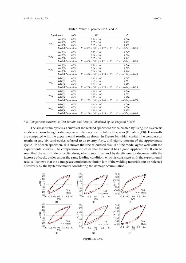
Appl. Sci. 2018, 8, 1701 19 of 24

Table 9. Values of parameters K’ and n’.

Specimens εB/% K’ n’

WA1

WA1(1) 0.25 2.26 × 107 0.546WA1(2) 0.35 2.65 × 107 0.499WA1(3) 0.45 3.05 × 107 0.459Model Parameters K′ = 3.95× 109εB + 1.27× 107 n′ = −43.5εB + 0.654

WA2


WA3


WB1

WB1(1) 0.25 1.40 × 107 0.567WB1(2) 0.35 1.63 × 107 0.521WB1(3) 0.45 1.86 × 107 0.475Model Parameters K′ = 2.30× 109εB + 8.25× 106 n′ = −46.0εB + 0.628

WB2


WB3


5.6. Comparison between the Test Results and Results Calculated by the Proposal Model

The stress-strain hysteresis curves of the welded specimens are calculated by using the hysteresismodel and considering the damage accumulation, constructed by this paper (Equation (13)). The resultsare compared with the experimental results, as shown in Figure 16, which contain the comparisonresults of any six semi-cycles referred to as twenty, forty, and eighty percent of the approximatecyclic life of each specimen. It is shown that the calculated results of the model agree well with theexperimental curves. The comparison indicates that the model has a good applicability. It can beseen that the amplitude of cyclic stress, elastic modulus, and hysteretic energy decrease with theincrease of cyclic cycles under the same loading condition, which is consistent with the experimentalresults. It shows that the damage accumulation evolution law of the welding materials can be reflectedeffectively by the hysteretic model considering the damage accumulation.


Model Parameters 79 1024.11000.4 ×+×=′ BK ε 649.00.41 +−=′ Bn ε

WB1

WB1(1) 0.25 1.40 × 107 0.567 WB1(2) 0.35 1.63 × 107 0.521 WB1(3) 0.45 1.86 × 107 0.475


WB2

WB2(1) 0.25 1.41 × 107 0.566 WB2(2) 0.35 1.63 × 107 0.521 WB2(3) 0.45 1.85 × 107 0.476


WB3

WB3(1) 0.25 1.40 × 107 0.566 WB3(2) 0.35 1.64 × 107 0.520 WB3(3) 0.45 1.86 × 107 0.475


5.6. Comparison between the Test Results and Results Calculated by the Proposal Model

The stress-strain hysteresis curves of the welded specimens are calculated by using the hysteresis model and considering the damage accumulation, constructed by this paper (Equation (13)). The results are compared with the experimental results, as shown in Figure 16, which contain the comparison results of any six semi-cycles referred to as twenty, forty, and eighty percent of the approximate cyclic life of each specimen. It is shown that the calculated results of the model agree well with the experimental curves. The comparison indicates that the model has a good applicability. It can be seen that the amplitude of cyclic stress, elastic modulus, and hysteretic energy decrease with the increase of cyclic cycles under the same loading condition, which is consistent with the experimental results. It shows that the damage accumulation evolution law of the welding materials can be reflected effectively by the hysteretic model considering the damage accumulation.

(a) (b) (c)

(d) (e) (f)

-0.3 -0.2 -0.1 0.0 0.1 0.2 0.3-400-300-200-1000100200300400

σ/MPa

ε/% Test Model -0.4 -0.2 0.0 0.2 0.4-450-300-1500

150300450

Test Model

σ/MPa

ε/% -0.4 -0.2 0.0 0.2 0.4-450-300-1500150300450 Test Model

ε/%

σ/MPa

-0.3 -0.2 -0.1 0.0 0.1 0.2 0.3-400-300-200-1000100200300400 Test Model

ε/%

σ/MPa

-0.4 -0.2 0.0 0.2 0.4-450-300-1500150300450

Test Model

σ/MPa

ε/% -0.4 -0.2 0.0 0.2 0.4-450-300-1500150300450 Test Model

σ/MPa

ε/%Figure 16. Cont.

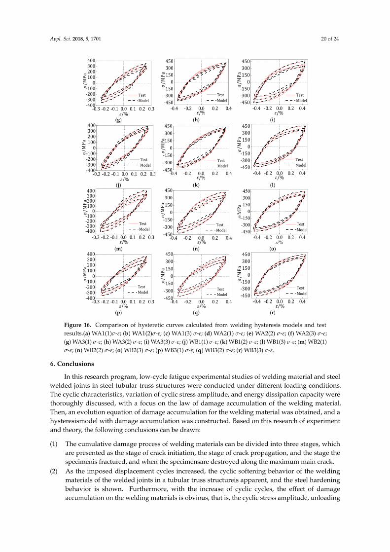
Appl. Sci. 2018, 8, 1701 20 of 24


(g) (h) (i)

(j) (k) (l)

(m) (n) (o)

(p) (q) (r)

Figure 16. Comparison of hysteretic curves calculated from welding hysteresis models and test results.(a) WA1(1)σ-ε; (b) WA1(2)σ-ε; (c) WA1(3) σ-ε; (d) WA2(1) σ-ε; (e) WA2(2) σ-ε; (f) WA2(3) σ-ε; (g) WA3(1) σ-ε; (h) WA3(2) σ-ε; (i) WA3(3) σ-ε; (j) WB1(1) σ-ε; (k) WB1(2) σ-ε; (l) WB1(3) σ-ε; (m) WB2(1) σ-ε; (n) WB2(2) σ-ε; (o) WB2(3) σ-ε; (p) WB3(1) σ-ε; (q) WB3(2) σ-ε; (r) WB3(3) σ-ε.

6. Conclusions

In this research program, low-cycle fatigue experimental studies of welding material and steel welded joints in steel tubular truss structures were conducted under different loading conditions. The cyclic characteristics, variation of cyclic stress amplitude, and energy dissipation capacity were thoroughly discussed, with a focus on the law of damage accumulation of the welding material. Then, an evolution equation of damage accumulation for the welding material was obtained, and a hysteresismodel with damage accumulation was constructed. Based on this research of experiment and theory, the following conclusions can be drawn:

-0.3 -0.2 -0.1 0.0 0.1 0.2 0.3-400-300-200-1000100200300400 Test Model

σ/MPaε/% -0.4 -0.2 0.0 0.2 0.4-450-300-1500150300450

Test Model

σ/MPa

ε/% -0.4 -0.2 0.0 0.2 0.4-450-300-1500150300450 Test Model

σ/MPa

ε/%

-0.3 -0.2 -0.1 0.0 0.1 0.2 0.3-400-300-200-1000100200300400 Test Model

σ/MPa

ε/% -0.4 -0.2 0.0 0.2 0.4-450-300-1500150300450

Test Model

σ/MPaε/% -0.4 -0.2 0.0 0.2 0.4-450-300-1500150300450

Test Model

σ/MPa

ε/%

-0.3 -0.2 -0.1 0.0 0.1 0.2 0.3-400-300-200-1000100200300400 Test Model

σ/MPa

ε/% -0.4 -0.2 0.0 0.2 0.4-450-300-1500150300450

Test Model

σ/MPa

ε/% -0.4 -0.2 0.0 0.2 0.4-450-300-150

0150300450

Test Modelσ/

MPa

ε/%

-0.3 -0.2 -0.1 0.0 0.1 0.2 0.3-400-300-200-1000100200300400 Test Model

σ/MPa

ε/% -0.4 -0.2 0.0 0.2 0.4-450-300-1500150300450

Test Model

σ/MPa

ε/% -0.4 -0.2 0.0 0.2 0.4-450-300-1500150300450 Test Model

σ/MPa

ε/%Figure 16. Comparison of hysteretic curves calculated from welding hysteresis models and testresults.(a) WA1(1)σ-ε; (b) WA1(2)σ-ε; (c) WA1(3) σ-ε; (d) WA2(1) σ-ε; (e) WA2(2) σ-ε; (f) WA2(3) σ-ε;(g) WA3(1) σ-ε; (h) WA3(2) σ-ε; (i) WA3(3) σ-ε; (j) WB1(1) σ-ε; (k) WB1(2) σ-ε; (l) WB1(3) σ-ε; (m) WB2(1)σ-ε; (n) WB2(2) σ-ε; (o) WB2(3) σ-ε; (p) WB3(1) σ-ε; (q) WB3(2) σ-ε; (r) WB3(3) σ-ε.

6. Conclusions

In this research program, low-cycle fatigue experimental studies of welding material and steelwelded joints in steel tubular truss structures were conducted under different loading conditions.The cyclic characteristics, variation of cyclic stress amplitude, and energy dissipation capacity werethoroughly discussed, with a focus on the law of damage accumulation of the welding material.Then, an evolution equation of damage accumulation for the welding material was obtained, and ahysteresismodel with damage accumulation was constructed. Based on this research of experimentand theory, the following conclusions can be drawn:

(1) The cumulative damage process of welding materials can be divided into three stages, whichare presented as the stage of crack initiation, the stage of crack propagation, and the stage thespecimenis fractured, and when the specimensare destroyed along the maximum main crack.

(2) As the imposed displacement cycles increased, the cyclic softening behavior of the weldingmaterials of the welded joints in a tubular truss structureis apparent, and the steel hardeningbehavior is shown. Furthermore, with the increase of cyclic cycles, the effect of damageaccumulation on the welding materials is obvious, that is, the cyclic stress amplitude, unloading

Appl. Sci. 2018, 8, 1701 21 of 24

stiffness, and energy dissipation capacity of the weldingmaterials degenerate gradually.Furthermore, the larger the controlled loading strain amplitude, the faster the rate of damageaccumulation. The amplitude of the loading strain has a greater effect on the welding material ofbase metal Q235 than that of base metal Q345.

(3) Based on the test results and Park–Ang model, an evolutionequation of damage accumulationfor welding materials is established considering both energy and deformation comprehensively,in which the energy part is no longer confined to the perfect elastic-plastic condition.Then, the value of parameter λ is fitted by the test data.

(4) It is revealed by the experimental research that the cyclic characteristic and constitutive behaviorof the welding material is quite different from the base metal, and the constitutive model used formonotonic loading cannot simulate the damage degradation behavior of the welding materialsunder cyclic loading. Therefore, a hysteresismodel with damage accumulation of weldingmaterials is constructed based on the Ramberg–Osgood model and the experimental results,which includedthe initial loading curve, cyclic stress-strain curve, and a model of the hystereticcurve. The model can reveal the effects of damage accumulation and the nonlinear constitutiverelation of the plasticstage.

(5) The damage parameters and model parameters η, ξ, g, h, K’ and n’ are fitted by the test results.The hysteretic curves calculated by the hysteretic model are compared with the test results, whichshow that the model has good applicability and the cumulative damage evolution law of thewelding materials reflected by the model is basically consistent with the test results.

Author Contributions: W.Y. designed the experiments. Y.S. and P.C. performed the experiments. Y.S. and W.Y.analyzed the data and wrote the paper.

Funding: This research was supported in part by The National Natural Science Foundation of China under Grant51468054 and in part by the Funding Project of First-Class Discipline Construction of Universities in Ningxia(Domestic First-Class Discipline Construction) under Grant NXYLXK2017A03.

Conflicts of Interest: The authors declare no conflict of interest.

References

1. Wardenier, J.; Packer, J.A.; Zhao, X.L.; Vegte, G.J.V.D. Hollow Sections in Structural Applications; Bouwen MetStaal: Rotterdam, The Netherlands, 2010.

2. Khademi, F. Load Rating of Railway Bridges by Analysis and Testing. Master’s Thesis, Illinois Institute ofTechnology, Chicago, IL, USA, 2015.

3. Khademi, F. Enhancing Load Rating of Railway Truss Bridges through a Hybrid Structural Analysis andinstrumentation Procedure. Ph.D. Thesis, Illinois Institute of Technology, Chicago, IL, USA, 2017.

4. Chen, Y.; Feng, R.; Gao, S.W. Experimental study of concrete-filled multiplanar circular hollow sectiontubular trusses. Thin-Walled Struct. 2015, 94, 199–213. [CrossRef]

5. Cui, C.; Zhang, Q.H.; Bao, Y.; Kang, J.P.; Bu, Y.Z. Fatigue performance and evaluation of welded joints insteel truss bridges. J. Constr. Steel Res. 2018, 148, 450–456. [CrossRef]

6. Gillman, A.; Fuchi, K.; Buskohl, P.R. Truss-based nonlinear mechanical analysis for origami structuresexhibiting bifurcation and limit point instabilities. Int. J. Solids Struct. 2018, 147, 80–93. [CrossRef]

7. Huang, W.J.; Fenu, L.G.; Chen, B.C.; Briseghella, B. Experimental study on joint resistance and failure modesof concrete filled steel tubular (cfst) truss girders. J. Constr. Steel Res. 2018, 141, 241–250. [CrossRef]

8. Ozyurt, E.; Wang, Y.C. Effects of non-uniform temperature distribution on critical member temperature ofsteel tubular truss. Eng. Struct. 2016, 116, 95–106. [CrossRef]

9. Tiainen, T.; Mela, K.; Jokinen, T.; Heinisuo, M. The effect of steel grade on weight and cost of warren-typewelded tubular trusses. Proc. Inst. Civ. Eng. Struct. Build. 2017, 170, 855–873. [CrossRef]

10. Van Der Kooi, K.; Hoult, N.A.; Le, H. Monitoring an in-service railway bridge with a distributed fiber opticstrain sensing system. J. Bridge Eng. 2018, 23, 05018007. [CrossRef]

11. Zhou, W.; Chen, Y.; Wang, K.; Han, S.; Galarza, F.P. Experimental research on circular concrete filled stainlesssteel tubular truss. Thin-Walled Struct. 2017, 117, 224–238. [CrossRef]

http://dx.doi.org/10.1016/j.tws.2015.04.013

http://dx.doi.org/10.1016/j.jcsr.2018.06.014

http://dx.doi.org/10.1016/j.ijsolstr.2018.05.011


http://dx.doi.org/10.1016/j.engstruct.2016.02.044

http://dx.doi.org/10.1680/jstbu.16.00112

http://dx.doi.org/10.1061/(ASCE)BE.1943-5592.0001281

http://dx.doi.org/10.1016/j.tws.2017.04.026

Appl. Sci. 2018, 8, 1701 22 of 24

12. Yang, W.W.; Wang, X.L.; Wang, D.D. Design of long-span and wave-shaped steel canopy structure of ningxiahelan mountain stadium. Adv. Mater. Res. 2011, 243–249, 72–78. [CrossRef]

13. Cui, W.; Wang, F. Damage Accumulation. In Encyclopedia of Tribology, 2013 Edition; Wang, Q.J.,Chung, Y.-W., Eds.; Springer: Boston, MA, USA, 2013; pp. 706–709.

14. Diel, S.; Huber, O. A continuum damage mechanics model for the static and cyclic fatigue of cellularcomposites. Materials 2017, 10, 951. [CrossRef] [PubMed]

15. Lian, J.H.; Jia, X.X.; Munstermann, S.; Bleck, W. A generalized damage model accounting for instability andductile fracture for sheet metals. Key Eng. Mater. 2014, 611–612, 106–110. [CrossRef]

16. Möller, B.; Baumgartner, J.; Wagener, R.; Kaufmann, H.; Melz, T. Low cycle fatigue life assessment of weldedhigh-strength structural steels based on nominal and local design concepts. Int. J. Fatigue 2017, 101, 192–208.[CrossRef]

17. Nie, G.B.; Fan, F.; Zhi, X.D. A constitutive model for circular steel pipe by spatial hysteretic test. Adv. Struct.Eng. 2012, 15, 1279–1290. [CrossRef]

18. Rong, J.; Kyriakides, S. Ratcheting, wrinkling and collapse of tubes under axial cycling. Int. J. Solids Struct.2009, 46, 2856–2870.

19. Whittaker, M.T.; Wilshire, B. Creep and creep fracture of 2.25cr–1.6w steels (grade 23). Mater. Sci. Eng. A2010, 527, 4932–4938. [CrossRef]

20. Du, G.F.; Huo, L.S.; Kong, Q.Z.; Song, G.B. Damage detection of pipeline multiple cracks using piezoceramictransducers. J. Vibroeng. 2016, 18, 2828–2838. [CrossRef]

21. Feng, Q.; Kong, Q.Z.; Song, G.B. Damage detection of concrete piles subject to typical damage types basedon stress wave measurement using embedded smart aggregates transducers. Measurement 2016, 88, 345–352.[CrossRef]

22. Feng, Q.; Xiao, H.; Kong, Q.Z.; Liang, Y.B.; Song, G.B. Damage detection of concrete piles subject to typicaldamages using piezoceramic based passive sensing approach. J. Vibroeng. 2016, 18, 801–812.

23. Ling, Y.B.; Li, D.S.; Song, G.B.; Zhan, C. Damage detection of shear buildings through structural mass-stiffnessdistribution. Smart Struct. Syst. 2017, 19, 11–20. [CrossRef]

24. Lu, G.T.; Li, Y.R.; Wang, T.; Xiao, H.; Huo, L.S.; Song, G.B. A multi-delay-and-sum imaging algorithm for damagedetection using piezoceramic transducers. J. Intell. Mater. Syst. Struct. 2017, 28, 1150–1159. [CrossRef]

25. Guo, Y.L.; Zhou, P.; Wang, M.Z.; Pi, Y.L.; Bradford, M.A. Numerical studies of cyclic behavior and designsuggestions on triple-truss-confined buckling-restrained braces. Eng. Struct. 2017, 146, 1–17. [CrossRef]

26. Li, Z.; Zhu, B.; Wu, L.; Han, Q. Experimental research on hysteretic behavior of unstiffened tubular n-joints.J. Build. Struct. 2008, 29, 69–74.

27. Yang, W.; Wang, X. Experimental research on seismic behavior of unstiffened overlapped chs k-joints.J. Build. Struct. 2013, 34, 85–92.

28. Yang, W.; Wang, X. Numerical analysis of hysteretic behavior of unstiffened overlapped chs k-joints in steelpipe structures by finite element method. J. Lanzhou Univ. Technol. 2012, 33, 009.

29. Wang, H.; Jing, H.; Zhao, L.; Han, Y.; Lv, X.; Xu, L. Dislocation structure evolution in 304l stainless steel andweld joint during cyclic plastic deformation. Mater. Sci. Eng. A 2017, 690, 16–31. [CrossRef]

30. Shen, Z.; Wu, A. Seismic analysis of steel structures considering damage cumulation. Front. Arch. Civ.Eng. China 2007, 1, 1–11. [CrossRef]

31. Shen, Z.Y. A cumulative damage model for the analysis of steel frames under seismic actions. In Proceedingsof the Advances in Steel Structures, Hong Kong, China, 15–17 December 1999; pp. 13–24.

32. Sun, Z.; Wang, X. Postbuckling investigations of piezoelectric microdevices considering damage effects.Sensors 2014, 14, 4876. [CrossRef] [PubMed]

33. Shi, Y.; Wang, M.; Wang, Y. Experimental and constitutive model study of structural steel under cyclicloading. J. Constr. Steel Res. 2011, 67, 1185–1197. [CrossRef]

34. Do, V.N.V.; Lee, C.H.; Chang, K.H. A constitutive model for uniaxial/multiaxial ratcheting behavior of aduplex stainless steel. Mater. Des. 2015, 65, 1161–1171.

35. Wang, M.; Fahnestock, L.A.; Qian, F.; Yang, W. Experimental cyclic behavior and constitutive modeling oflow yield point steels. Constr. Build. Mater. 2017, 131, 696–712. [CrossRef]

36. Nip, K.H.; Gardner, L.; Davies, C.M.; Elghazouli, A.Y. Extremely low cycle fatigue tests on structural carbonsteel and stainless steel. J. Constr. Steel Res. 2009, 66, 96–110. [CrossRef]

http://dx.doi.org/10.4028/www.scientific.net/AMR.243-249.72

http://dx.doi.org/10.3390/ma10080951

http://www.ncbi.nlm.nih.gov/pubmed/28809806

http://dx.doi.org/10.4028/www.scientific.net/KEM.611-612.106

http://dx.doi.org/10.1016/j.ijfatigue.2017.02.014

http://dx.doi.org/10.1260/1369-4332.15.8.1279

http://dx.doi.org/10.1016/j.msea.2010.04.033

http://dx.doi.org/10.21595/jve.2016.17040

http://dx.doi.org/10.1016/j.measurement.2016.01.042

http://dx.doi.org/10.12989/sss.2017.19.1.011

http://dx.doi.org/10.1177/1045389X16666184


http://dx.doi.org/10.1016/j.msea.2017.02.090

http://dx.doi.org/10.1007/s11709-007-0001-7

http://dx.doi.org/10.3390/s140304876



http://dx.doi.org/10.1016/j.conbuildmat.2016.11.035


Appl. Sci. 2018, 8, 1701 23 of 24

37. Basan, R.; Franulovic, M.; Prebil, I.; Kunc, R. Study on ramberg-osgood and chaboche models for42crmo4 steel and some approximations. J. Constr. Steel Res. 2017, 136, 65–74. [CrossRef]

38. Dundu, M. Evolution of stress-strain models of stainless steel in structural engineering applications.Constr. Build. Mater. 2018, 165, 413–423. [CrossRef]

39. Hassanein, M.F.; Elchalakani, M.; Karrech, A.; Patel, V.I.; Yang, B. Behaviour of concrete-filled double-skinshort columns under compression through finite element modelling: Shs outer and shs inner tubes. Structures2018, 14, 358–375. [CrossRef]

40. Marohnic, T.; Basan, R.; Franulovic, M. Evaluation of methods for estimation of cyclic stress-strain parametersfrom monotonic properties of steels. Metals 2017, 7, 15. [CrossRef]

41. Szymczak, C.; Kujawa, M. Torsional buckling and post-buckling of columns made of aluminium alloy.Appl. Math. Model. 2018, 60, 711–720. [CrossRef]

42. Zappalorto, M.; Maragoni, L. Nonlinear mode iii crack stress fields for materials obeying a modifiedramberg-osgood law. Fatigue Fract. Eng. Mater. Struct. 2018, 41, 708–714. [CrossRef]

43. Ramberg, W.; Osgood, W.R. Description of Stress-Strain Curves by Three Parameters; Technical Note;NationalAdvisory Committee for Aeronautics: Washington, DC, USA, 1943.

44. Corigliano, P.; Crupi, V.; Fricke, W.; Friedrich, N.; Guglielmino, E. Experimental and numerical analysis offillet-welded joints under low-cycle fatigue loading by means of full-field techniques. Proc. Inst. Mech. Eng.Part C J. Mech. Eng. Sci. 2015, 229, 1327–1338. [CrossRef]

45. Aucott, L.; Huang, D.; Dong, H.B.; Wen, S.W.; Marsden, J.; Rack, A.; Cocks, A.C.F. A three-stage mechanisticmodel for solidification cracking during welding of steel. Met. Mater. Trans. A Phys. Met. Mater. Sci. 2018,49A, 1674–1682. [CrossRef]

46. Borgesen, P.; Wentlent, L.; Khasawneh, S.; Shirazi, S.; Schmitz, D.; Alghoul, T.; Greene, C.; Yin, L. A mechanisticthermal fatigue model for snagcu solder joints. J. Electron. Mater. 2018, 47, 2526–2544. [CrossRef]

47. Mac Ardghail, P.; Harrison, N.; Leen, S.B. A through-process, thermomechanical model for predictingwelding-induced microstructure evolution and post-weld high-temperature fatigue response. Int. J. Fatigue2018, 112, 216–232. [CrossRef]

48. Markiewicz, E.; Langrand, B.; Notta-Cuvier, D. A review of characterisation and parameters identificationof materials constitutive and damage models: From normalised direct approach to most advanced inverseproblem resolution. Int. J. Impact Eng. 2017, 110, 371–381. [CrossRef]

49. Peng, Y.; Wu, C.; Gan, J.; Dong, J. Determination of the local constitutive properties of the welded steel jointsusing digital image correlation method. Constr. Build. Mater. 2018, 171, 485–492. [CrossRef]

50. Wang, X.L.; Yang, W.W.; Zou, L. Finite element analysis for unstiffened overlapped chs kk-joints welded indifferent ways. Adv. Mater. Res. 2011, 163–167, 299–306. [CrossRef]

51. Brünig, M.; Gerke, S. Simulation of damage evolution in ductile metals undergoing dynamic loadingconditions. Int. J. Plast. 2011, 27, 1598–1617. [CrossRef]

52. Cheng, C.; Li, X. Cyclic experimental studies on damage evolution behaviors of shale dependent on structuralorientations and confining pressures. Energies 2018, 11, 160. [CrossRef]

53. Ku-Herrera, J.; Pacheco-Salazar, O.; Ríos-Soberanis, C.; Domínguez-Rodríguez, G.; Avilés, F. Self-sensing ofdamage progression in unidirectional multiscale hierarchical composites subjected to cyclic tensile loading.Sensors 2016, 16, 400. [CrossRef] [PubMed]

54. Mielke, A. Complete-damage evolution based on energies and stresses. Discret. Contin. Dyn. Syst. Ser.S (DCDS-S) 2012, 4, 423–439.

55. Murakami, S.; Kamiya, K. Constitutive and damage evolution equations of elastic-brittle materials based onirreversible thermodynamics. Int. J. Mech. Sci. 1997, 39, 473–486. [CrossRef]

56. Chinese Code. Gb/700-2006 Carbon Structural Steel; Standards Press of China: Beijing, China, 2006.57. Chinese Code. Jgj81-2002 Technical Specification for Welding of Steel Structure of Building; Standards Press of

China: Beijing, China, 2003.58. Park, Y.J.; Ang, H.S. Mechanistic seismic damage model for reinforced concrete. J. Struct. Eng. 1985, 111,

722–739. [CrossRef]59. Krajcinovic, D. Damage Mechanics; Elsevier: New York, NY, USA, 1996; pp. 117–197.60. Shi, G.; Gao, Y.; Wang, X.; Zhang, Y. Mechanical properties and constitutive models of low yield point steels.

Constr. Build. Mater. 2018, 175, 570–587. [CrossRef]



http://dx.doi.org/10.1016/j.istruc.2018.04.006

http://dx.doi.org/10.3390/met7010017

http://dx.doi.org/10.1016/j.apm.2018.03.040

http://dx.doi.org/10.1111/ffe.12730

http://dx.doi.org/10.1177/0954406215571462

http://dx.doi.org/10.1007/s11661-018-4529-z

http://dx.doi.org/10.1007/s11664-018-6121-0

http://dx.doi.org/10.1016/j.ijfatigue.2018.02.015

http://dx.doi.org/10.1016/j.ijimpeng.2017.01.028


http://dx.doi.org/10.4028/www.scientific.net/AMR.163-167.299

http://dx.doi.org/10.1016/j.ijplas.2011.02.003

http://dx.doi.org/10.3390/en11010160

http://dx.doi.org/10.3390/s16030400


http://dx.doi.org/10.1016/S0020-7403(97)87627-8

http://dx.doi.org/10.1061/(ASCE)0733-9445(1985)111:4(722)


Appl. Sci. 2018, 8, 1701 24 of 24

61. Shi, G.; Wang, M.; Bai, Y.; Wang, F.; Shi, Y.; Wang, Y. Experimental and modeling study of high-strengthstructural steel under cyclic loading. Eng. Struct. 2012, 37, 1–13. [CrossRef]

62. Christ, H.J.; Mughrabi, H. Cyclic stress-strain response and microstructure under variable amplitude loading.Fatigue Fract. Eng. Mater. Struct. 1996, 19, 335–348. [CrossRef]

63. Mayer, T.; Mazza, E.; Holdsworth, S.R. Parameter evolution in a continuous masing approach for cyclicplasticity and its physical interpretation. Mech. Mater. 2013, 57, 86–96. [CrossRef]

64. Segalman, D.J.; Starr, M.J. Inversion of masing models via continuous iwan systems. Int. J. Non-Linear Mech.2007, 43, 74–80. [CrossRef]

65. Siddiquee, M.S.A. A pressure-sensitive kinematic hardening model incorporating masing’s law. Acta Geotech.2015, 10, 623–642. [CrossRef]

© 2018 by the authors. Licensee MDPI, Basel, Switzerland. This article is an open accessarticle distributed under the terms and conditions of the Creative Commons Attribution(CC BY) license (http://creativecommons.org/licenses/by/4.0/).


http://dx.doi.org/10.1111/j.1460-2695.1996.tb00971.x

http://dx.doi.org/10.1016/j.mechmat.2012.10.014

http://dx.doi.org/10.1016/j.ijnonlinmec.2007.10.005

http://dx.doi.org/10.1007/s11440-015-0375-y

http://creativecommons.org/

http://creativecommons.org/licenses/by/4.0/.

Study on Hysteresis Model of Welding Material in ...

Documents

Transcript of Study on Hysteresis Model of Welding Material in ...