STUDY OF THE PARABOLIC AND ELLIPTIC APPROACHES VALIDITIES...

Mahmoud, H., et al.: Study of the Parabolic and Elliptic Approaches Validities for … THERMAL SCIENCE, Year 2012, Vol. 16, No. 1, pp. 223-238 223

STUDY OF THE PARABOLIC AND ELLIPTIC APPROACHES

VALIDITIES FOR A TURBULENT CO-FLOWING JET

by

Houda MAHMOUD a*

, Wassim KRIAA a, Hatem MHIRI

a,

Georges Le PALEC b, and Philippe BOURNOT

b

a Unité de thermique et thermodynamique des procédés industriels, Ecole Nationale d’Ingénieurs de Monastir, Monastir, Tunisie

b IUSTI, UMR CNRS, Marseille, France

Original scientific paper DOI: 102298/TSCI101104097M

An axisymmetric turbulent jet discharged in a co-flowing stream was studied with the aid of parabolic and elliptic approaches. The simulations were performed with two in-house codes. Detailed comparisons of data show good agreement with the corresponding experiments; and different behaviors of jet dilution were found in initial region at different ranges of velocities ratios. It has been found that the two approaches give practically the same results for the velocities ratios Ru ≤ 1.5. Further from this value, the elliptic approach highlights the appearance of the fall velocity zone and that’s due to the presence of a trough low pressure. This fall velocity has not been detected by the parabolic approach and that’s due to the jet entrainment by the ambient flow. The intensity of this entrainment is di-rectly related to the difference between the primary (jet) and the secondary flow (co-flow). In fact, by increasing the velocities ratios Ru, the sucked flux by the outer stream becomes more important; the fall velocity intensifies and changes into a recirculation zone for Ru 5.

Key words: axisymmetric jet, turbulence, co-flow, recirculation zone, parabolic approach, elliptic approach

Introduction

The turbulent jets emerged in a moving stream exist widely in nature as well as in

propulsion systems, reactors, engines, etc. The ability to predict the turbulent mixing in flows

with complex features is vital for modeling the dynamics of such flows and a prerequisite for

predicting turbulent combustion situation [1].

In this context, several experimental [2-5] and numerical [6-8] works have been

devoted. The experiments on co-flowing jets have been piloted since 1973, with low

velocities ratios (Ru ranging between 0.01 and 0.33). The purpose is to solve the seeding

problems found at the jet edge and to avoid the oscillations development in the primary flow.

Antonia et al. [2] were the first who led an experimental study on turbulent jets emerged in a

co-flow with velocities ratios ranging between 0.22 and 0.33. These authors have shown that

*nCorresponding author; e-mail: [email protected]

Mahmoud, H., et al.: Study of the Parabolic and Elliptic Approaches Validities for … 224 THERMAL SCIENCE, Year 2012, Vol. 16, No. 1, pp. 223-238

such flow does not reach an asymptotic state. Afterwards, Nickels et al. [3] proved the

existence of the self-similarity zone. They showed that, for a velocity ratio Ru = 0.09, the

radial profiles of the mean streamwise velocity collapse fairly well far downstream (x/d = 30). Also, they noted that the flow becomes independent from initial conditions at an axial

distance strongly depending on initial momentum. Mesnier [4] investigated three turbulent

jets, including helium, air and CO2 jets exiting with 40 m/s velocity in a low-speed air co-

flow. He was concerned to study density and nozzle geometry effects on jet structure. Antoine

et al. [5] performed measurements in turbulent water jet flowing with an injection velocity

equal to 10 m/s and emerging in a low-speed co-flow water (Ru = 0.05). They showed that co-

flow reduces the jet spreading rate by approximately 30% from the free jet.

Numerically, the study of turbulent jets emerging in a co-flow with low velocities

ratios has been the subject of several works [6-7] in order to stabilize the calculations and to

ensure the codes convergence. These studies, conducted with small velocities ratios (0.01 ≤ Ru

≤ 0.2), are based on the elliptic (complete equations) or parabolic approach (boundary layer

assumptions). Imine et al. [6] performed their numerical simulation on an axisymmetric isothermal and turbulent jet discharged in a co-flow at a velocity ratio Ru equal to 0.01.

They used the elliptic approach and the second order model. These authors are interested to

study the nozzle geometry and the densities ratios influence on the jet mixing rate and on

mean and turbulent flow parameters. They showed that the asymmetric geometry improve the

mixing process of the turbulent co-flowing jet. Habli et al. [7] used the parabolic approach,

the first and the second order model to study an axisymmetric turbulent jet moving in a co-

flow with different velocities ratios (Ru ranging between 0 and 0.2). They focused their work

on the test of Reynolds Stress algebraic Model performance compared to that of the standard

k-e model in predicting the average and the turbulent flow sizes in free and forced convection

modes. Also, they are interested to the influence of the velocities ratios on the jet typical

parameters and self-similarity zone. These authors showed that the two considered models

give similar results in forced convection mode. In contrast, in free convection mode, the

second order model is better than the k-e model in modeling buoyancy and turbulence

structures.

This bibliographic review shows that all experimental and numerical studies have

considered low velocities ratios Ru ranging between 0.01 and 0.33. However, a co-flowing jet

with large velocities ratios is a new method of flame stabilization [8] and a desire of many

industrial applications. In this context, in our last publication [9] we studied an axisymmetric

turbulent jet discharging into co-flowing stream with different velocities ratios ranging

between 0 and . The results showed that the two turbulence models: standard k- and the

Reynolds stress model (RSM) are valid to predict the average and turbulent flow sizes. Also,

the effect of the velocities ratios on the flow structure was examined. It is noted, for Ru > 1,

the appearance of a fall velocity zone due to the presence of a trough low pressure. This fall

velocity becomes increasingly intense according to Ru and changes into a recirculation zone

for Ru 4.5.

In this paper, we propose to study the limit of the parabolic approach validity

compared to the elliptic one, to predict the turbulent co-flowing jet structure for a large range

of velocities ratios (Ru varied between 0 and 10). The resolution of the governing equations

was performed by two computer codes: the first code use the elliptic approach (complete

equations governing the flow without the boundary layer approximations) while the second

code is based on the parabolic approach (equations with boundary layer assumptions).


Numerical modeling

Assumptions

The flow configuration and the associated parameters used in the present study are

the same as those used by Mesnier [4] for its measurements (fig. 1). A turbulent jet, with a

discharge velocity U0, issues out from a circular nozzle of diameter d equal to 7 mm, in a co-

-flowing atmosphere of the same fluid which has a velocity U. The flow is assumed to be

incompressible, axisymmetric, and mean steady in nature. The Reynolds number Re = u0d/

is assumed large enough for the flow to be fully turbulent at the considered distances from the

nozzle. A cylindrical co-ordinate system may be used, with x the axial position, originating

from the nozzle, and r the radial distance from the nozzle axis.

Figure 1. Grid and domain of the studied configuration; (a) grid of the elliptic approach, (b) grid of the

parabolic approach

Governing equations

Based on the above assumptions and the following dimensionless variables (1), the

Reynolds-averaged Navier-Stokes (RANS) equations written in cylindrical co-ordinates were

used by the parabolic and elliptic approaches.

2 3 20 0 0 0

, , , , , ,x r u v k εd p

X R U V K E Pd d u u u u ρu

(1)

For the elliptic approach and according to the Reynolds averaged decomposition, the

transport equations can be written as:


( ) ( )

0RU RV

X R

(2)

( ) 1 ( ) 1( ) ( )

UU RVU PU U RU V

X R R X X R R

(3)

( ) 1 ( ) 1

( ) ( )UV RVV P

U V RV VX R R R X R R

(4)

Taking into account that the two models: standard k-e and RSM predict well the

characteristic sizes of the turbulent co-flowing jet [7, 9] and the standard k-e model is

inexpensive and easy to implement, it will be adopted in this work.

The dimensionless turbulent kinetic energy and dissipation rate equations can be

written in the following way:

k

t k t k

( ) 1 1 1( )

Re Re

UK K R KRVK P E

X R R X X R R R

s s (5)

2

1 k 2

t t

1 1 1( )

Re Re

UE E R E E ERVE C P C

X R R X X R R R K K

(6)

Pk is the production term of the turbulent kinetic energy given by the following

relation:

2 2 2 2

t

12

ReK

U V V U VP

X R R X R

(7)

We note that the Reynolds constraints tensor terms i jU U (i, j = 1 or 2) are modelled

by the approximations proposed by Martynenko et al. [10]. The constants numerical values of

the standard k-e model are given in tab. 1 [11].

For the parabolic approach, we

used the standard k-e model by

considering the boundary layer

approximations. These equations

are given by Habli et al. [7].

Dimensionless boundary conditions

The dimensionless boundary (8) and inlet (9) conditions are written into the follow-

ing way:

For X > 0:

u

0 for 0

, 0, , for

U K E PV R

R R R R

U R P K K E E R

(8)

Table 1.Empirical constants of the standard k-e model [11]

Cm Ck s C1 C2 sk

0.09 1.0 1.3 1.44 1.92 1


In this study, we considered several types of emission conditions. The following

system gives the uniforms’ velocity profile:

For X= 0:

0 0

u

= 0, 1, , for 0 1/2

= 0, , , , = 0 for 1/2

V U K K E E R

V U R K K E E P R

(9)

The inlet turbulent kinetic energy k0 is deduced from the turbulent intensity I (10)

given by Mesnier [4], I = 4.17%:

20 0

3( )

2k Iu (10)

For a jet with an axial symmetry, the inlet dissipation rate of the turbulent kinetic

energy is calculated by the relation [12]:

30

0

k

l

(11)

The turbulence length scale l is a physical quantity related to the size of the large

eddies that contain the energy in turbulent flows. In the axisymmetric jet, l is restricted by the

half of the nozzle diameter.

The turbulent kinetic energy K and the dissipation rate E at the co-flow emission

are calculated by the correlations [13]:

23

2k u I (12)

3 34

0.07

C k

l

(13)

The experimental emission profiles of Mesnier [4] and Antoine et al. [5] were used

to study the validity of the elaborated codes with velocities ratios Ru, equal to 0.01 and 0.05,

respectively.

Numerical method

The numerical resolution of the elliptic approach eq. (2-6) associated to their

boundary and emission conditions (8-9) was carried out by an in-house code based on a finite

volume method and a SIMPLE algorithm resolution. The transport equations were discretized

using a hybrid scheme and a staggered grid. This method was adopted for numerical stability

reasons. The idea is to evaluate scalar variables, such as pressure, at ordinary nodal points but

to calculate velocity components on staggered grids centred on the cell faces, (fig. 1(a). In

fact, the axial velocity cell is centred at the nodes (i + 1/2, j), the radial component cell at the

nodes (i, j + 1/2), whereas the pressure term, the kinetic energy and the dissipation rate are

centred at the nodes (i, j). For all the treated cases, the investigation domain dimensions according to X and R

depend on the injection velocities ratios Ru (50 ≤ X ≤ 160 and 30 ≤ R ≤ 60). Indeed, the

domain is very undersized when the velocity is extremely high.


In the longitudinal and transverse directions, the used grid is not uniform. Indeed,

the step was taken very small in the nozzle vicinity (DX » DR »10–2

). A little further, the step

of calculation increased (110 RX ), fig. 1(a).

To improve the accuracy of the numerical results for the elliptic approach, we con-

ducted a series of grid independency tests for each set velocity ratio. For Ru = 0.01, we

applied the test for three additional grids: (1) a coarse mesh with 504 277 nodes; (2) a me-

dium mesh with 504 427 nodes; and (3) a more refinement mesh with 558 427 nodes. We

can observe in fig. 2(a) that the passage through the grid refinement from the coarse grid to

the medium grid caused big difference in the predicted relative pressure. However, the cal-

culations using the fine mesh (558 427) gives similar results as using the medium grid (504

427). Thus, we presumed that the results obtained on the (504 427) mesh do not depend

on the grid. Therefore, we conducted all the simulations with the medium grid 504 427.

For the parabolic approach, the numerical resolution of the system equations was

carried out using another in-house code based on a finite difference method with a shifted

grid. In fact, the transport equations of momentum, energy, turbulent kinetic energy, and its

dissipation were discretized at the nodes (i + 1/2, j), whereas the continuity equation was

discretized at the nodes (i + 1/ 2, j + 1/2). The obtained discretized equations are then solved

by adopting a non-linear Gauss Seidel method [11] used in a former work [12]. This method

was adopted for numerical stability reasons as compared to a non-shifted grid method.

In the longitudinal direction, the used grid is not uniform. In this direction, we tested

different steps (fig. 2(b)). Then, we showed that taking ΔX1 = 0.001 for X < 5 and ΔX2 = 0.01

for X > 5 is sufficient to obtain a numerical solution independent of the grid. In the transverse

direction, the used grid is uniform and the calculation step was constant (DR = 10–2

). Its value

imposed a sufficient number of points in this direction, so that the jet was not cut.

For the two approaches, the obtained equations were solved line by line using the

tri-diagonal matrix algorithm (TDMA). The convergence of the calculations was obtained

when the sum of normalized residues was less than 10–5

. In fact, when the discretized

equation is written as: apfp = Sanbfnb + Sf, the normalized residue is the difference between

the two terms of this equation divided by p pp

a :

p p

nb nb p pnoeudP nb

n

p

a S a

Ra

where p is the variable U, V, K, or E in the node, anb and ap – the coefficients of the

discretized equation, and S – the source term of this equation.

Results and discussion

The first stage of calculation consisted primarily in testing the developed programs

based on parabolic and elliptic approaches. To validate our numerical computations, the

obtained results are compared with the experimental data of Mesnier [4] and Antoine et al. [5]. Then, we undertook a parametric study of the two approaches ability in depicting the co-

flowing stream effects on the behavior of the jet flow.


Comparaison between computation results and experimental data

Two in-house codes were developed in order to study the behavior of the co-flowing

jet under large range of velocities ratios. The first code is developed to solve the parabolic

approach equations and the second is elaborated to solve the elliptic approach equations. To

validate these two codes, the calculated mean quantities were compared to the results of

Mesnier [4] proposed in initial and intermediate regions and with the results of Antoine et al. [5] given in the developed zone.

The initial conditions used for the validation with the experimental data of Mesnier

[4] correspond to a velocities ratio Ru equal to 0.01 and a Reynolds number equal to 23115. In

this case, the calculations started from an axial distance X = 0.3. To compare our numerical

simulation with the experimental data of Antoine et al. [5], we used an initial velocities ratio

Ru = 0.05, a fully developed velocity profile at the nozzle exit and a Reynolds number Re =

=10000.

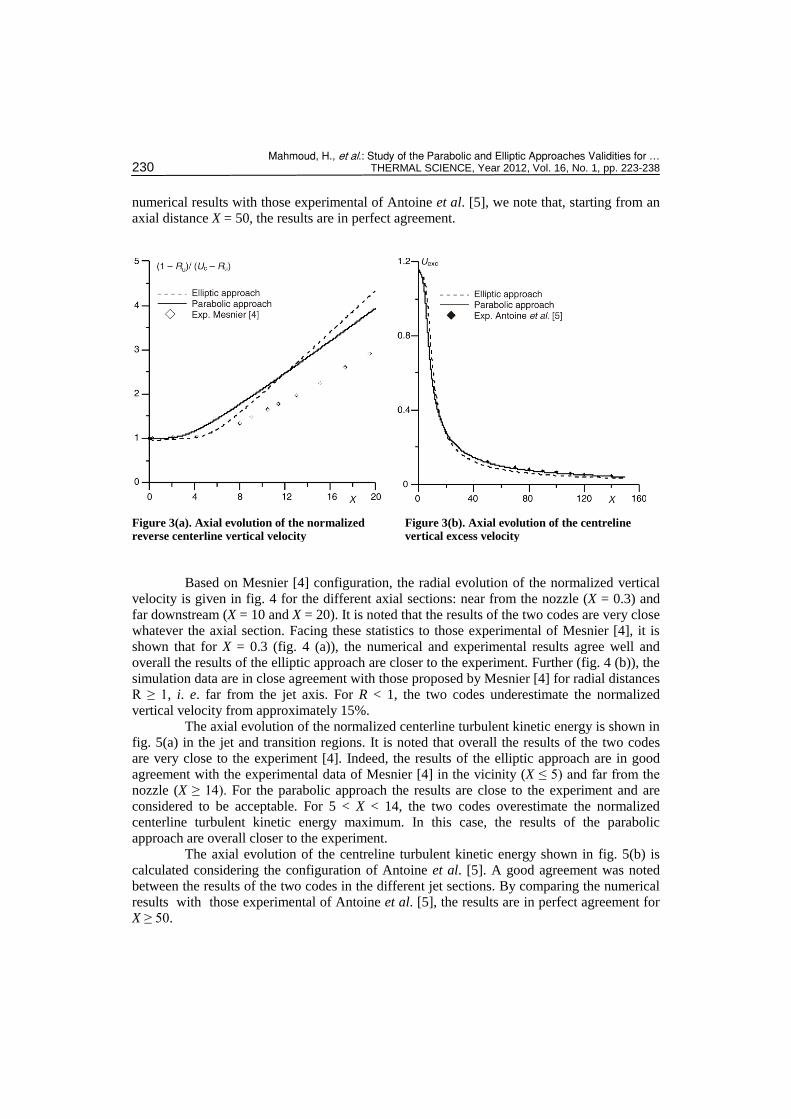
In fig. 3(a), we represented the axial evolution of the normalized centerline vertical

velocity in the two first zones. It is noted that, overall, the results of the two codes are very

close and satisfactory. In fact, closely to the nozzle X ≤ 2, the results of the two codes are

similar and agree well with the experimental data of Mesnier [4]. For X > 2, a small

difference, which does not exceed 2% is observed between the results of the two codes. The

comparison between the experimental data of Mesnier [4] and our numerical results showed

that, for 2 < X ≤ 12, the elliptic approach results are closer to those experimental. On the other

hand, for X > 12, the results of the parabolic approach are closest with those of experiment.

Nevertheless, the differences between the experimental and numerical results remain

acceptable and can be explained by experiment errors [4, 6] quoted in former work.

The streamwise distribution of the centreline vertical excess velocity Uexc (Antoine

et al. [5] configuration) is presented in fig. 3(b). It illustrates a satisfactory agreement between

the results of the two computer codes in the different flow regions. By comparing the

Figure 2. Effect of the grid on the centreline; (a) relative pressure (elliptic approach), (b) vertical velocity (parabolic approach)


numerical results with those experimental of Antoine et al. [5], we note that, starting from an

axial distance X = 50, the results are in perfect agreement.

Figure 3(a). Axial evolution of the normalized reverse centerline vertical velocity

Figure 3(b). Axial evolution of the centreline vertical excess velocity

Based on Mesnier [4] configuration, the radial evolution of the normalized vertical

velocity is given in fig. 4 for the different axial sections: near from the nozzle (X = 0.3) and

far downstream (X = 10 and X = 20). It is noted that the results of the two codes are very close

whatever the axial section. Facing these statistics to those experimental of Mesnier [4], it is

shown that for X = 0.3 (fig. 4 (a)), the numerical and experimental results agree well and

overall the results of the elliptic approach are closer to the experiment. Further (fig. 4 (b)), the

simulation data are in close agreement with those proposed by Mesnier [4] for radial distances

R ≥ 1, i. e. far from the jet axis. For R < 1, the two codes underestimate the normalized

vertical velocity from approximately 15%.

The axial evolution of the normalized centerline turbulent kinetic energy is shown in

fig. 5(a) in the jet and transition regions. It is noted that overall the results of the two codes

are very close to the experiment [4]. Indeed, the results of the elliptic approach are in good

agreement with the experimental data of Mesnier [4] in the vicinity (X ≤ 5) and far from the

nozzle (X ≥ 14). For the parabolic approach the results are close to the experiment and are

considered to be acceptable. For 5 < X < 14, the two codes overestimate the normalized

centerline turbulent kinetic energy maximum. In this case, the results of the parabolic

approach are overall closer to the experiment.

The axial evolution of the centreline turbulent kinetic energy shown in fig. 5(b) is

calculated considering the configuration of Antoine et al. [5]. A good agreement was noted

between the results of the two codes in the different jet sections. By comparing the numerical

results with those experimental of Antoine et al. [5], the results are in perfect agreement for

X ≥ 50.


Figure 4. Radial evolution of the normalized vertical velocity

Figure 5. (a) Axial evolution of the normalized centerline turbulent kinetic energy, (b) Axial evolution of

the centerline turbulent kinetic energy

So, we can conclude that the numerical results of the two codes obtained using the

parabolic and elliptic approach are very close and practically similar. The comparison

between the numerical and experimental data of [4] and [5] in the three jet areas, show a very

acceptable and satisfactory agreement which validates the two calculations codes.

Study of the co-flowing jet structure using the

parabolic and elliptic approaches

In this section, we focus on the behavior of the co-flowing jet under a velocities

ratios change by the aid of the parabolic and elliptic approaches. The calculations were carried

out using the geometrical configuration of Mesnier [4] and the uniform emission profiles.


Study of the characteristic sizes of the flow

The comparison between the characteristic sizes of a co-flowing jet obtained by

parabolic and elliptic approaches are investigated in this section, for different velocities ratios

ranging between 0 and 10 and a Reynolds number Re equal to 23115. The main idea was to

study the ability of the parabolic approach compared to the elliptic one to predict the co-flowing

jet structure for all considered velocities ratios.

The axial evolution of the centerline vertical velocity Uc is given in fig. 6 for

different velocities ratios Ru. For Ru ≤ 1.5, fig. 6(a), it is noted that the parabolic and elliptic

approaches give similar results in the nozzle vicinity (initial zone of the jet). Nevertheless, the

potential core length given by the elliptic approach is slightly greater than that of the parabolic

approach. In the transition zone, whatever the value of Ru, a small difference which does not

exceed 5% is observed between the results of the two approaches. In fact, more Ru moves

away from 1 (Ru → 0 or Ru →1.5), more this difference is remarkable but always lower than

5%. In the developed region, the two approaches give the same results. Thus, we can conclude that for velocities ratios Ru ≤ 1.5, the two approaches give results practically similar and acceptable in the different jet regions, which confirms the validity of the parabolic approach. In fig. 6(b), we show the axial evolution of the centerline vertical velocity Uc for different velocities ratios Ru respectively equal to 2, 3.5, and 4.5. It is noted

that the elliptic approach highlights in the nozzle vicinity an abrupt fall of the velocity which

isn’t visible by parabolic calculation. This fall takes values greater than zero and becomes

more intense when Ru is larger. This phenomenon is ascribable with a non-compensation of

the momentum loss due to the trough of low pressure created by the secondary flow (co-flow),

fig. 7(b). Further, in the established zone, the results of the two approaches become similar.

Thus, we confirm that when Ru is greater than 1.5, the parabolic approach becomes inapt to

predict the characteristic of the co-flowing jet especially the fall velocity marked by the

elliptic approach. In fig. 6(c), we represent the evolution of Uc for different velocities ratios

equal to 5, 7, and 10, respectively. By comparing the results of the two approaches, we note

that the elliptic approach shows an abrupt fall of the centerline vertical velocity to reach a

minimal value Ucmin. (appearance of the recirculation bubble), before growing for tending

towards the co-flow velocity. This fall is more intense when Ru is larger. This recirculation

zone that has not been detected by the parabolic approach is due to the use of the boundary

layer approximations unable to describing the recirculation zone in the nozzle vicinity. So, for

this flow regime, the parabolic approach is inapt to predict the structure of the jet discharged

into a co-flow.

The axial evolutions of the centerline relative pressure determined by the parabolic

and elliptic approaches for different velocities ratios Ru, are presented in fig. 7. It is noted that

for the parabolic approach Pc is almost constant and equal to zero for the different velocities

ratios. For Ru 1.5, fig. 7(a), it is shown with the elliptic approach that the dimensionless

centerline relative pressure is about 10–3

in the nozzle vicinity and tends towards zero for the

great values of X. So, the pressure is very low and almost equal to zero in the all calculation

field. In this case, the small depression detected in the nozzle vicinity does not have an effect

on the vertical velocity, fig. 6(a), which explains the absence of the fall velocity in this zone.

For 1.5 < Ru < 5, fig. 7(b), the centerline relative pressure takes important negative values in

the nozzle vicinity (about 10–1

), from where appear the fall velocity, fig. 6(b). In fact, as Ru

increases as the depression becomes more important and the fall velocity intensifies in the


Figure 6. Axial evolution of the centerline vertical velocity, (a) Ru ≤ 1.5, (b) 1.5 < Ru < 5, (c) Ru ≥ 5

Figure 7. Axial evolution of the centreline relative pressure, (a) Ru ≤ 1.5, (b) 1.5 < Ru < 5, (c) Ru ≥ 5


nozzle vicinity. Just afterwards, the centerline pressure increases to reach a maximum which depends on Ru and then tends towards zero downstream the nozzle. For Ru ≥ 5, fig.

7(c), the depression detected in the nozzle vicinity becomes more intense and is at the

origin of the velocity drop and hence the appearance of a recirculation bubble on the jet axis,

fig.7(b).

Visualization of the turbulent co-flowing jet structure

using the parabolic and elliptic approaches

To study the stream structure and the different flow regimes using the parabolic and

elliptic approaches, the vertical velocity contours and the streamlines are presented in fig. 8,

Figure 8. Vertical velocity contours and streamlines for the first case; depression without effect on

velocity (Ru ≤ 1.5)


9, and 10 for a broad range of velocities ratios Ru ranging between 0 and 10 (the jet velocity is

taken constant and equal to 40 m/s) and a Reynolds number equal to 23115. From these

figures, we can distinguish three cases: the first case where the depression is without any

effect on the velocity (regime without recirculation bubble), 0 ≤ Ru ≤ 1.5 (fig. 8). In the

second case, the depression is with an effect on the velocity (regime without recirculation

bubble), 1.5 < Ru <5 (fig. 9) and the third case where the depression is with recirculation

bubble (regime with recirculation bubble), Ru ≥ 5 (fig.10).

Figure 9. Vertical velocity contours and streamlines for the second case; depression with effect on velocity (1.5 < Ru < 5)

The results of the parabolic and elliptic approaches were compared in fig. 8, for

three velocities ratios Ru respectively equal to 0, 0.5, and 1.5. We note that the two

approaches give very close results and when Ru recedes from 1 (Ru → 0 or Ru → 1.5), the

differences between the contours become noticeable but stay acceptable, fig. 6(a). In this


Case (Ru ≤ 1.5), the boundary layer assumptions (parabolic approach) are considered valid,

which is in agreement with the previous works who have adopted the parabolic approach to

study the turbulent free jets [12] and the co-flowing jets [6-8] moving with low velocities ratios Ru ≤ 0.2.

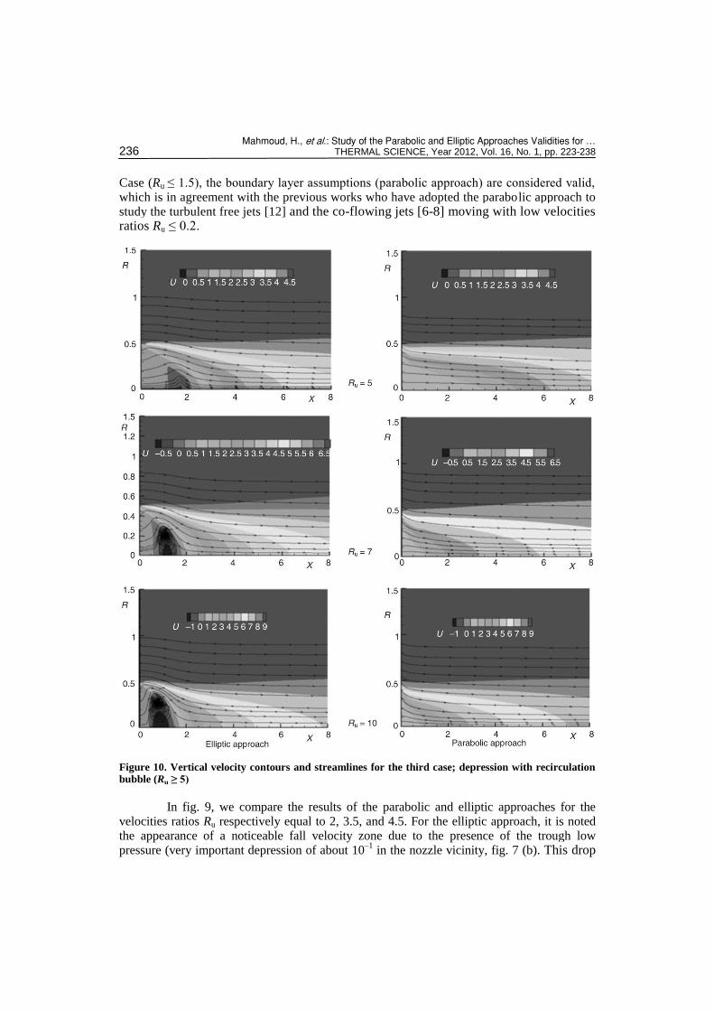
Figure 10. Vertical velocity contours and streamlines for the third case; depression with recirculation bubble (Ru ≥ 5)

In fig. 9, we compare the results of the parabolic and elliptic approaches for the

velocities ratios Ru respectively equal to 2, 3.5, and 4.5. For the elliptic approach, it is noted

the appearance of a noticeable fall velocity zone due to the presence of the trough low

pressure (very important depression of about 10–1

in the nozzle vicinity, fig. 7 (b). This drop


that has not been seen by the parabolic approach is due to the phenomenon of the jet training by the outer stream. The intensity of this training is directly related to the difference

between the primary (jet) and the secondary flow (co-flow). In fact, for the great velocities

ratios, the sucked flux by the co-flow becomes more important and the fall velocity

intensifies. Also, we note that when the fall velocity is important, the streamlines are very

deformed. Thus, we conclude that the parabolic approach becomes unable to predict and to

describe the structure of the co-flowing jet when Ru is greater than 1.5.

The flow regime with depression and recirculation bubble (Case 3) is shown in fig.

10 for the velocities ratios Ru respectively equal to 5, 7, and 10. The comparison between the

results of the elliptic and parabolic approaches shows that when Ru increases, the elliptic

approach highlights a recirculation zone which moves from the jet axis towards the outer

nozzle edge. This recirculation zone that has not been detected by the parabolic approach is

explained by the fact that the mass fluid provided by jet is not sufficient any more for the

secondary flow when Ru ≥ Ruc = 5, which creates a return of the downstream fluid. Thus, a

negative vertical velocity zone is observed: this is the recirculation bubble. Moreover, the

comparison between the streamlines of the two approaches shows that close to the nozzle, the

elliptic approach streamlines are completely deformed compared to those of the parabolic

approach. This character is due to the presence of recirculation zone. Thus, for this flow

regime, the difference between the two approaches become obvious and the parabolic

approach is inapt to describe the structure of the jet emerging in a co-flowing stream.

Conclusions

In the present paper, a detailed comparison has been made for many statistical

quantities, such as the axial evolution of mean streamwise velocity, turbulent kinetic energy,

as well as radial profiles of vertical velocity. The agreement between simulation and

experiment is generally very good for the elliptic and parabolic approaches. In the near filed,

the numerical results deviate somewhat from the experimental data of Mesnier, presumably

due to imperfection in the experiment.

According to the velocities ratio Ru, three cases and two flow regimes are identified:

a depression produced without any effect on the velocity for 0 ≤ Ru ≤ 1.5 (Case 1: regime

without recirculation bubble). A drop pressure which is accompanied with an effect on the

velocity for 1.5 < Ru < 5 (Case 2: regime without recirculation bubble). Finally, the depression

has an influence on the velocity and displays a recirculation bubble for 5 ≤ Ru ≤ 10 (Case 3:

regime with recirculation bubble). The origin of these two regimes is the entrainment between the jet and the ambient

stream. The intensity of this phenomenon is related to the velocities difference. In fact, for the

greatest velocities ratios, the sucked flux by the secondary stream becomes more important

and the fall velocity intensifies. For Ru Ruc = 5, this depression is sufficient to have a

negative fall velocity and generate the recirculation bubble which migrates to the nozzle

extremity according to the value of Ru. The comparison between the results of the two approaches showed that the

phenomena identified by the elliptic approach in both cases 2 and 3 are invisible by the

parabolic approach. This concluded the validity of the parabolic approach compared to the

elliptic one which is limited to the first case (depression without effect on the velocity) i. e.

for 0 ≤ Ru ≤ 1.5. In fact, for Ru > 1.5, the parabolic approach becomes unable to predict and to

describe the structure and the characteristic parameters of the co-flowing jet.


References

[1] Benarous, A., Liazid, A., H2-O2 Supercritical Combustion Modeling Using a CFD code, Thermal Science, 13 (2009), 3, pp. 139-152

[2] Antonia, R. A., Bilger, R. W., An Experimental Investigation of an Axisymmetric Jet in a Co-Flowing Air Stream, Journal of fluid Mechanics, 61 (1973), 4, pp. 805-822

[3] Nickels, T. B., Perry, A. E., An Experimental and Theoretical Study of the Turbulent Coflowing Jet, Journal Fluid Mechanics, 309 (1996), pp. 157-182

[4] Mesnier, B., Studies on the Development of Turbulent Jets with Variable Density in Axisymmetric and Asymmetric Geometries (In Frensh), Ph. D. thesis, Orleans University, Orleans, France, 2001

[5] Antoine, Y., Fabrice, L., Michel, L., Turbulent Transport of a Passive Scalar in a Round Jet Discharging into a Co-Flowing Stream, Journal Mechanics B. Fluids, 20 (2001), 2, pp. 275-301

[6] Imine, B., et al., Study of Non-Reactive Isothermal Turbulent Asymmetric Jet with Variable Density, Comput. Mechanics, 38 (2006), 2, pp. 151-162

[7] Habli, S., et al., Influence of a Coflowing Ambient Stream on a Turbulent Axisymmetric Buoyant Jet, Journal Heat Transfer, 130 (2008), 2, pp. 1-15

[8] Wei-Biao, F., et al. The Use of Co-Flowing Jets with Large Velocity Differences for the Stabilization of Low Grade Coal Flames, Proceedings, 26st Symposium (International) on Combustion, Naples, Italy, The Combustion Institute, Pittsburgh, Penn., USA, 1987, pp. 567-574

[9] Mahmoud, H., et al., A Numerical Study of a Turbulent Axisymmetric Jet Emerging in a Co-Flowing Stream, Energy Conversion and Management, 51 (2010), 11, pp. 2117-2126

[10] Martynenko, O. G., Korovkin, V. N., Flow and Heat Transfer in Round Vertical Buoyant Jets, Interna-tional Journal Heat Mass Trans, 37 (1994), 1, pp. 51-58

[11] Hossain, M. S., Rodi, W., A Turbulent Model for Boyant Flows and Its Application to Vertical Boyant Jets, Pergamon, New York, USA, 1982, pp. 121-178

[12] Habli, S., Mhiri, H., Golli, S., Numerical Study of Inflow Conditions on an Axisymmetric Turbulent Jet turbulent, International Journal Thermal Science, 40 (2001), 5, pp. 497-511

[13] ***, Fluent Incorporated 6.2.16.

Paper submitted: November 12, 2010 Paper revised: October 6, 2011 Paper accepted: October 6, 2011

Nomenclature

d – nozzle diameter, [m] k – turbulent kinetic energy, [m2s2] P – static pressure, [Pa] r – transverse co-ordinates Re – Reynolds number (= ud/n), [–] Ru – velocities ratio (= u/ u0), [–] U, V – dimensionless mean velocity components, [–] Uex – excess velocity (Uex = U – U), [–] u, v – mean velocity components along x and – y-directions, [ms–1] x – longitudinal co-ordinate, [m]

Greeks symbols

e – dissipation rate of the turbulent – kinetic energy, [m2s–3]

n – molecular kinematic viscosity, [ m2s–1] – density, [kgm–3]

Subscripts

C – jet axis – ambient middle 0 – nozzle exit

Superscripts

– – Reynolds average ' – fluctuation

STUDY OF THE PARABOLIC AND ELLIPTIC APPROACHES VALIDITIES...

Documents

Transcript of STUDY OF THE PARABOLIC AND ELLIPTIC APPROACHES VALIDITIES...