Study of the influence of bed roughness on the flow ...

Wouter Callewaert, Brecht Versteele

characteristics of an open channel confluenceStudy of the influence of bed roughness on the flow

Academic year 2013-2014Faculty of Engineering and ArchitectureChairman: Prof. dr. ir. Peter TrochDepartment of Civil Engineering

Master of Science in Civil EngineeringMaster's dissertation submitted in order to obtain the academic degree of

Counsellors: Ir. Stéphan Creëlle, Ir. Laurent SchindfesselSupervisor: Prof. dr. ir. Tom De Mulder

Foreword

During the first master year of Civil Engineering, our interest in hydraulic engineering grew. This

common interest resulted in the choice of a master dissertation in the field of hydraulics and we were

delighted with the assignment of this subject: “Study of the influence of bed roughness on the flow

characteristics of an open channel confluence”. The balance between performing experiments and

processing of results created an enjoyable working schedule. The difference in interpreting

measurement data and theory gave us a challenging year but also a very interesting one from which we

learned a lot. Getting used to both aspects of experimental research presented itself to be very

enriching.

We would like to express our sincere gratitude to the people who have supported us. First we would

like to thank our promoter, prof. dr. ir. Tom De Mulder, for giving us the opportunity to conduct this

master dissertation and for all his support. Our gratitude also goes to our supervisor ir. Stéphan

Creëlle for his guidance and feedback during the year. His expertise on the subject helped a lot for the

realization of this master dissertation. Furthermore, we would like to thank ir. Laurent Schindfessel

for his practical tips, handy tools, and support during the year.

Finally, we would like to thank our parents for the support and trust they gave us during our study of

Civil Engineering.

Wouter Callewaert & Brecht Versteele

Ghent, June 2014

Deze pagina is niet beschikbaar omdat ze persoonsgegevens bevat.Universiteitsbibliotheek Gent, 2021.

This page is not available because it contains personal information.Ghent University, Library, 2021.

Overview

Study of the influence of bed roughness on the flow characteristics of an

open channel confluence

Wouter Callewaert, Brecht Versteele

Supervisor: Prof. dr. ir. Tom De Mulder

Counsellors: Ir. Stéphan Creëlle, Ir. Laurent Schindfessel

Master's dissertation submitted in order to obtain the academic degree of

Master of Science in Civil Engineering

Department of Civil Engineering

Chairman: Prof. dr. ir. Peter Troch

Faculty of Engineering and Architecture

Academic year 2013-2014

Keywords:

Open channel confluence, flow characteristics, experimental, bed roughness, artificial grass

Study of the influence of bed roughness on

the flow characteristics of an open channel

confluence

Wouter Callewaert and Brecht Versteele

Supervisor: prof. dr. ir. Tom De Mulder

Abstract: An experimental study on a 90° open

channel confluence is performed to investigate the

influence of bed roughness on the flow characteristics.

To this end, artificial grass, which acts as a well-

submerged vegetation, is put on the channel bottom to

increase the bed roughness. Measurement data is

gathered from both configurations and compared. From

this comparison, it was found that the velocity

distribution over the channel depth changes for the grass

configuration. Because of this rearrangement, higher

velocities are present at the water surface and the

dimensions of the separation zone change. Furthermore,

the width of the mixing layer develops in a different way

when going downstream and a different overall flow

pattern is obtained.

Keywords: Open channel confluence, flow

characteristics, experimental, bed roughness, artificial

grass, mixing layer, zone of separation

I. INTRODUCTION

Open channel confluences are very common in

nature whereby every river consists of a main channel

and some tributaries. Since this is a very important

part of the river, it has already led to numerous

studies presented in literature. The main flow features

of a confluence (Figure 1) are a stagnation zone at the

upstream corner, a zone of separation just

downstream of the tributary, a contracted flow region

between the separation zone and the wall opposing

the tributary and a mixing layer.

Figure 1: flow characteristics in an open channel

confluence

The zone of separation is an area just downstream

of the junction where the flow has a small velocity

and where recirculation exists. It is created by the

momentum of the side flow which causes the main

flow to detach at the downstream corner of the

junction. Studies (Shumate, 1998; Best and Reid,

1984) have shown that the separation zone is

significantly longer and wider at the surface level than

at the bottom[1] [2].

L. Crombé (2013) also indicated with numerical simulations that the friction coefficient is a determining parameter [3]. The dimensions of the

zone of separation decrease with increasing bed

friction. Furthermore, the dimensions of this zone

decrease when the flow ratio from the main channel to

the downstream channel increases. The presence of

the separation zone forces the water from both

channels to pass a smaller zone. This contracted

region will have bigger downstream velocities

because the same amount of water has to pass a

smaller zone. The aim of the present paper is to investigate the

influence of bed roughness on these flow

characteristics. To increase the friction factor at the

bottom, the flume is equipped with a cover of

artificial grass. The grass blades of this cover have an

average height of 3cm. In the past, the flume without

the grass cover has already been discussed by

Schindfessel et al. (2014) and will be used as

benchmark [4].

II. LABORATORY EXPERIMENTS

A. Experimental set-up

The experiments were performed at the hydraulics

laboratory of Ghent. The open channel facility

consists of a 90° channel confluence with a chamfered

rectangular cross-section with concrete walls. The

main channel has a length of 33.18m. The tributary is

5.17m long and intersects with the main channel at

13.12m (measured from upstream). Both channels

have a constant width Wd of 0.98m. The coordinate

system originates at the upstream corner of the

junction. The x-axis is orientated along the main

channel towards upstream while the y-axis is pointing

in the downstream direction of the tributary.

The coordinates are always represented

dimensionless by dividing them by the channel width

Wd. The discharge ratio q* is defined as:

(1)

Where Qm and Qt denote the incoming discharge of

the main channel and the tributary respectively, Qd

expresses the downstream discharge and is the sum of

the discharge of both inlet channels. The downstream

discharge Qd of 40 l/s together with a constant

downstream water level hd of 0.415m yields to a

constant downstream Froude number Frd of 0.05. This

value is typical for lowland rivers [5]. The choice for

q* = 0.25 was based on the value of the reference

case.

Schindfessel et al. (2014) carried out their

experiments in the same experimental set-up, with

equal geometrical and flow parameters. As flumes

with a chamfered rectangular cross-section are quite

uncommon in literature, a comparison was made with

the experiments of Shumate (1998). The latter carried

out his experiments in the Iowa Institute of Hydraulic

Research. The flume has similar dimensions but the

cross-section is not chamfered. Moreover, total

discharge and velocity are higher than in the present

study. As a consequence of the lower velocities in the

present experiments, water level differences will be

negligible. According to Schindfessel et al. (2014),

one of the main differences due to the chamfers, is the

depth of the zone of separation. This zone does not

gradually decrease in width towards the bottom, like

observed by Shumate, but has a vertical interface that

ends abruptly at z/Wd = 0.1 (just above the chamfer).

B. Measurement methodology

Flow velocities at the water surface are measured

using large scale surface particle image velocimetry

(LSSPIV). Therefore a 1920x1080 pixel camera is

placed at a fixed height above the water surface,

taking images at a rate of 15Hz. The fluid is seeded

with a tracing material that is recognizable by the

camera. The applied material consists of

polypropylene particles, covered in a white coating.

The duration of the recording is fixed at 180 seconds,

this results in the best equilibrium between quality

and quantity of the measurements. The processing

from frames to velocity data is done with the freeware

PIVlab 1.32.

To create velocity profiles in a cross-section of the

flume the ‘Vectrino II Profiling Velocimeter’ is used.

This device is a high-resolution acoustic Doppler

velocimeter (ADV) that can be used to measure

turbulence and velocities in 3D. Based on

observations from Schindfessel et al. (2014), a

measurement duration of 2min was chosen as

sufficient to obtain time-averaged velocities. To

obtain an accurate velocity profile over the entire

cross-section, nine vertical lines are measured where

each line consists of 15 measurement points. By

interpolation between the measured data, an

approximate plot is obtained with velocities for the

entire cross-section.

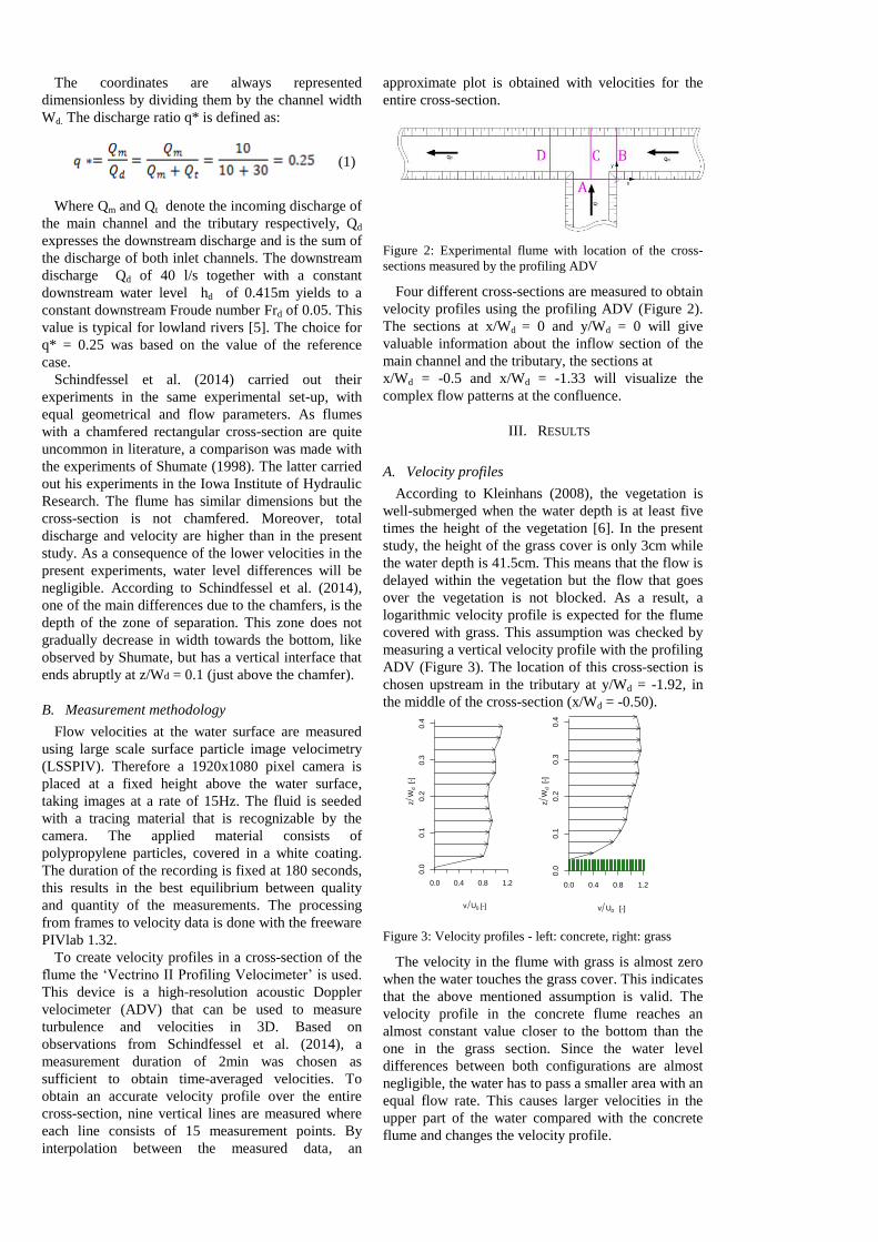
Figure 2: Experimental flume with location of the cross-

sections measured by the profiling ADV

Four different cross-sections are measured to obtain

velocity profiles using the profiling ADV (Figure 2).

The sections at x/Wd = 0 and y/Wd = 0 will give

valuable information about the inflow section of the

main channel and the tributary, the sections at

x/Wd = -0.5 and x/Wd = -1.33 will visualize the

complex flow patterns at the confluence.

III. RESULTS

A. Velocity profiles

According to Kleinhans (2008), the vegetation is

well-submerged when the water depth is at least five

times the height of the vegetation [6]. In the present

study, the height of the grass cover is only 3cm while

the water depth is 41.5cm. This means that the flow is

delayed within the vegetation but the flow that goes

over the vegetation is not blocked. As a result, a

logarithmic velocity profile is expected for the flume

covered with grass. This assumption was checked by

measuring a vertical velocity profile with the profiling

ADV (Figure 3). The location of this cross-section is

chosen upstream in the tributary at y/Wd = -1.92, in

the middle of the cross-section (x/Wd = -0.50).

0.0 0.4 0.8 1.2

0.0

0.1

0.2

0.3

0.4

v U0 [-]

zW

d [-]

0.0 0.4 0.8 1.2

0.0

0.1

0.2

0.3

0.4

v U0 [-]

zW

d [-]

Figure 3: Velocity profiles - left: concrete, right: grass

The velocity in the flume with grass is almost zero

when the water touches the grass cover. This indicates

that the above mentioned assumption is valid. The

velocity profile in the concrete flume reaches an

almost constant value closer to the bottom than the

one in the grass section. Since the water level

differences between both configurations are almost

negligible, the water has to pass a smaller area with an

equal flow rate. This causes larger velocities in the

upper part of the water compared with the concrete

flume and changes the velocity profile.

B. General velocity patterns

The main effect of the placement of the grass cover

is a rearrangement of the velocity distribution. This

difference is more pronounced in the tributary

because its discharge is three times larger than the one

of the main channel.

Due to the larger velocities in the tributary, the flow

enters the confluence with a larger force and pushes

the fluid from the main channel further to the outer

side. The separation zone increases in width and

decreases in length (Figure 4). This is partly

contradictory with the literature which predicts that

both the length and the width of the separation zone

decrease with increasing friction coefficient. It can be

concluded that the altered velocity distribution

obtained through the grass cover will dominate the

flow characteristics.

Figure 4: Vector plots obtained with the LSSPIV showing

velocity patterns – top: concrete, bottom: grass (The dotted

contour line indicates points with a longitudinal velocity of

zero).

Cross-sectional plots at x/Wd = -1.33 are shown in

Figure 5. For the flume with the grass cover, the

separation zone extends vertically but ends already at

mid-depth (z/Wd = 0.20). Lateral inflow from the

tributary collides with the flow of the main channel,

bends downward and is redirected towards the left

bank. This is probably the reason for the abrupt end

of the separation zone at a depth of z/Wd = 0.20. This

phenomenon does not appear in the concrete flume

because here, the cross-sectional velocities are

smaller and have not the power to reach the left bank

after the collision with the stream of the main channel,

instead the main flow redirects them downstream. The

highest upstream velocities, in the separation zone,

appear at the water surface and decrease in magnitude

when moving towards the bottom.

Figure 5: Cross-sectional plots at x/Wd = -1.33 with

longitudinal velocity (color scale) and cross-sectional

velocity (arrows) – Top: concrete, bottom: grass

C. Mixing and shear layer

The mixing layer width δ is defined as the ratio

between the outer velocity difference ΔU and the

maximum velocity gradient of the cross-section:

(2)

The width of the mixing layer is shown in Figure 6

and initially increases for both configurations (The

flow direction is from right to left). For the concrete

flume, the width of the mixing layer decreases again

from x/Wd = -0.45 while for the flume with the grass

cover, it increases until a value of x/Wd = -0.6

where it seems to remain constant. These results agree

well with the trend observed by Mignot et al. (2013)

[7]. This plateau is related to the strong lateral

confinement of the flow when it reaches the

confluence.

Figure 6: Mixing layer width

The instability of the shear layers was investigated

by means of vorticity plots and optical observations.

The vorticity of the shear layer starting at the

upstream corner was low in comparison with the shear

layer at the separation zone. These values are

confirmed with the optical observations. A lot of

vortices are shed from the downstream corner while

this is not the case for the upstream corner. As a

consequence only the shear layer at the separation

zone is unstable. The optical observations also

pointed out that the size of these vortices increase

over a longer distance at the grass flume.

IV. CONCLUSIONS

Experiments were performed to investigate the

influence of bed roughness on the flow characteristics

at a 90° confluence. The grass cover that was placed

on the channel bottom was small enough to presume

well-submerged vegetation. By equipping the flume

with this grass cover, the available cross-section for

the fluid to pass decreased. This resulted in an altered

velocity distribution. This difference was more

pronounced in the tributary because its discharge was

three times higher. As a result, the separation zone

could develop more in width and its length decreased

Measurement data from the profiling ADV showed

that the depth of the recirculation zone is limited by

the effect of the chamfers and the return flow to the

left bank located just above the channel bottom.

Furthermore, the mixing layer is wider in the grass

configuration and will extend further downstream

before both streams are mixed completely. At last,

optical observations showed that only the shear layer

starting at the downstream corner was unstable. The

instability arose as vortices that were shed and grew

along the shear plane.

REFERENCES

[1] E.D. Shumate, ‘Experimental description of flow at an

open-channel junction’, Unpublished Master thesis.

University of Iowa, 1998

[2] J.L. Best and I. Reid, ‘Separation zone at open channel

confluences’, Journal of Hydraulic Engineering, Vol.

110,11,1588-1594, 1984

[3] L. Crombe, S. Creelle, T.D.Mulder, Numerieke modellering

van een riviersamenvloeiing: Onderzoek naar de invloed van

vegetatie op de stromingspatronen(thesis).” 2013.

[4] L. Schindfessel, S. Creëlle, T. Boelens and T. De Mulder,

‘Flow patterns in an open channel confluence with a small

ratio of main channel to tributary discharge, Hydraulics

laboratory, Department of Civil Engineering, Ghent

University, Belgium, 2014

[5] Khublaryan, 2009, Surface Waters: Rivers, Streams, Lakes

and Wetlands. In Types and properties of water. Oxford:

EOLSS Publishers Co. Ltd.

[6] M. Kleinhans, Hydraulic roughness, 2008

Last visited December 2, 2013, from Utrecht University,

Faculty of Geosciences.

Web site:

www.geog.uu.nl/fg/mkleinhans/teaching/rivmorrough.pdf

[7] E. Mignot, I. Vinkovic, D. Doppler, N. Riviere, ‘Mixing

layer in open-channel junction flows’, Environmental Fluid

Mech, 2013

http://www.geog.uu.nl/fg/mkleinhans/teaching/rivmorrough.pdf

Studie van de invloed van bodemruwheid op

de stromingskarakteristieken van een

samenvloeiing van open kanalen

Wouter Callewaert en Brecht Versteele

Promotor: prof. dr. ir. Tom De Mulder

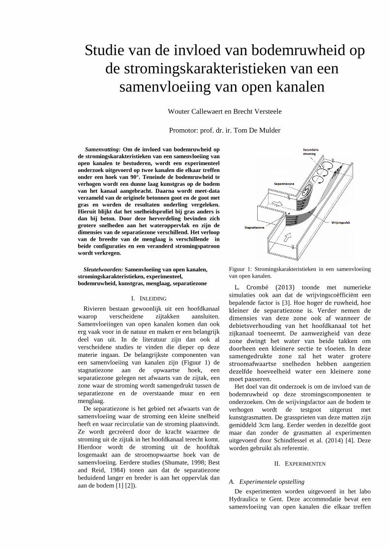
Samenvatting: Om de invloed van bodemruwheid op

de stromingskarakteristieken van een samenvloeiing van

open kanalen te bestuderen, wordt een experimenteel

onderzoek uitgevoerd op twee kanalen die elkaar treffen

onder een hoek van 90°. Teneinde de bodemruwheid te

verhogen wordt een dunne laag kunstgras op de bodem

van het kanaal aangebracht. Daarna wordt meet-data

verzameld van de originele betonnen goot en de goot met

gras en worden de resultaten onderling vergeleken.

Hieruit blijkt dat het snelheidsprofiel bij gras anders is

dan bij beton. Door deze herverdeling bevinden zich

grotere snelheden aan het wateroppervlak en zijn de

dimensies van de separatiezone verschillend. Het verloop

van de breedte van de menglaag is verschillende in

beide configuraties en een veranderd stromingspatroon

wordt verkregen.

Sleutelwoorden: Samenvloeiing van open kanalen,

stromingskarakteristieken, experimenteel,

bodemruwheid, kunstgras, menglaag, separatiezone

I. INLEIDING

Rivieren bestaan gewoonlijk uit een hoofdkanaal

waarop verscheidene zijtakken aansluiten.

Samenvloeiingen van open kanalen komen dan ook

erg vaak voor in de natuur en maken er een belangrijk

deel van uit. In de literatuur zijn dan ook al

verscheidene studies te vinden die dieper op deze

materie ingaan. De belangrijkste componenten van

een samenvloeiing van kanalen zijn (Figuur 1) de

stagnatiezone aan de opwaartse hoek, een

separatiezone gelegen net afwaarts van de zijtak, een

zone waar de stroming wordt samengedrukt tussen de

separatiezone en de overstaande muur en een

menglaag.

De separatiezone is het gebied net afwaarts van de

samenvloeiing waar de stroming een kleine snelheid

heeft en waar recirculatie van de stroming plaatsvindt.

Ze wordt gecreëerd door de kracht waarmee de

stroming uit de zijtak in het hoofdkanaal terecht komt.

Hierdoor wordt de stroming uit de hoofdtak

losgemaakt aan de stroomopwaartse hoek van de

samenvloeiing. Eerdere studies (Shumate, 1998; Best

and Reid, 1984) tonen aan dat de separatiezone

beduidend langer en breder is aan het oppervlak dan

aan de bodem [1] [2]).

Figuur 1: Stromingskarakteristieken in een samenvloeiing

van open kanalen.

L. Crombé (2013) toonde met numerieke

simulaties ook aan dat de wrijvingscoëfficiënt een

bepalende factor is [3]. Hoe hoger de ruwheid, hoe kleiner de separatiezone is. Verder nemen de dimensies van deze zone ook af wanneer de debietsverhouding van het hoofdkanaal tot het zijkanaal toeneemt. De aanwezigheid van deze zone dwingt het water van beide takken om doorheen een kleinere sectie te vloeien. In deze samengedrukte zone zal het water grotere stroomafwaartse snelheden hebben aangezien dezelfde hoeveelheid water een kleinere zone moet passeren.

Het doel van dit onderzoek is om de invloed van de

bodemruwheid op deze stromingscomponenten te

onderzoeken. Om de wrijvingsfactor aan de bodem te

verhogen wordt de testgoot uitgerust met

kunstgrasmatten. De grassprieten van deze matten zijn

gemiddeld 3cm lang. Eerder werden in dezelfde goot

maar dan zonder de grasmatten al experimenten

uitgevoerd door Schindfessel et al. (2014) [4]. Deze

worden gebruikt als referentie.

II. EXPERIMENTEN

A. Experimentele opstelling

De experimenten worden uitgevoerd in het labo

Hydraulica te Gent. Deze accommodatie bevat een

samenvloeiing van open kanalen die elkaar treffen

onder een hoek van 90°. De doorsnede bestaat uit een

afgeschuinde rechthoekige sectie met betonnen

muren. De lengte van het hoofdkanaal is 33.18m. De

zijtak is 5.17m lang en snijdt het hoofdkanaal op een

afstand van 13.12m (van opwaarts gemeten). Beide

kanalen hebben een constante breedte Wd van 0.98m.

De oorsprong van het assenstelsel is gepositioneerd

aan de stroomopwaartse hoek van de samenvloeiing.

De x-as is georiënteerd langs het hoofdkanaal, gericht

naar opwaarts, en de positieve zin van de y-as is

gericht in de afwaartse zin van de zijtak. De

coördinaten worden dimensieloos weergegeven door

ze te delen door de kanaalbreedte. De

debietsverhouding q* wordt gedefinieerd als:

(1)

Met Qd en Qt respectievelijk het instromend debiet

van de hoofdtak en de zijtak. Qd is het afwaartse

debiet wat de som is van de debieten van beide

instroomkanalen. Het afwaartse debiet Qd van 40 l/s

samen met de constante stroomafwaartse waterhoogte

hd van 0.415m leidt tot een constant stroomafwaarts

Froude nummer Frd van 0.05. Deze waarde is

typisch voor laagland rivieren [5]. De keuze voor

q* = 0.25 was gebaseerd op de waarde uit het

referentiegeval.

Schindfessel et al. (2014) voerden experimenten uit

in dezelfde experimentele opstelling, met dezelfde

geometrische - en stromingskarakteristieken.

Aangezien goten met een afgeschuinde doorsnede vrij

ongewoon zijn in de literatuur, wordt een vergelijking

gemaakt met de experimenten van Shumate (1998).

Die laatste voerde zijn experimenten uit in het

hydraulisch onderzoeksinstuut te Iowa. De goot daar

heeft gelijkaardige dimensies maar de doorsnede is

niet afgeschuind. Bovendien zijn het totale debiet en

de snelheden groter dan in de huidige studie. Als

gevolg van de lagere snelheden in de huidige studie

zijn de waterhoogteverschillen verwaarloosbaar.

Volgens Schindfessel et al., is één van de grootste

verschillen, veroorzaakt door de afschuiningen, de

diepte van de separatiezone. De breedte van deze

zone neemt niet geleidelijk af naar de bodem toe,

zoals waargenomen was door Shumate, maar heeft

een verticaal raakvlak dat abrupt stopt op z/Wd = 0.1

(Net boven de afschuining).

B. Meetmethode

Met de LSSPIV (Large scale surface particle image

velocimetry) worden stromingssnelheden aan het

wateroppervlak gemeten. Hiervoor wordt een

1920x1080 pixel camera op een vaste hoogte boven

het wateroppervlak geplaatst die beelden neemt met

een frequentie van 15Hz. Het water oppervlak wordt

bestrooid met een materiaal dat herkenbaar is voor de

camera. Dit materiaal bestaat uit polypropyleen

deeltjes die bedekt zijn met een witte deklaag. De

duur van een opname is 180 seconden, dit resulteert

in het beste evenwicht tussen de kwaliteit en

kwantiteit van de metingen. De verwerking van de

beelden naar snelheidsdata wordt uitgevoerd met de

freeware PIVlab 1.32.

Om een snelheidsprofiel te verkrijgen in een

doorsnede van de goot wordt de ‘Vectrino II Profiling

Velocimeter’ gebruikt. Dit toestel is een hoge-

resolutie akoestische Doppler Velocimeter ADV) die

kan gebruikt worden om turbulentie en snelheden in

3D te meten. Een meetduur van 2min werd, via

observaties van Schindfessel et al. (2014), als

voldoende beschouwd om tijdsgemiddelde snelheden

te verkrijgen. Om een nauwkeurig snelheidsprofiel

over de volledige doorsnede te verkrijgen zijn 9

verticale lijnen opgemeten waarbij elke lijn bestaat uit

15 meetpunten. Via interpolatie tussen de gemeten

data kan een benaderende plot verkregen worden met

snelheden over de volledige doorsnede.

Vier verschillende doorsnedes werden opgemeten

met de ADV om een snelheidsprofiel te verkrijgen.

De secties op

x/Wd = 0 en y/Wd = 0 geven belangrijke informatie

over de instroming uit het hoofd -en zijkanaal. De

secties x/Wd = -0.5 en x/Wd = -1.33 dienen om de

complexe stromingsprocessen te visualiseren die

optreden aan de samenvloeiing.

Figuur 2: Experimentele goot met de locatie van de

doorsneden die opgemeten worden met de ADV

III. RESULTATEN

A. Snelheidsprofielen

Volgens Kleinhans (2008) wordt vegetatie als

“voldoende onder water” beschouwd wanneer de

waterdiepte ten minste vijf keer de vegetatiehoogte is

[6]. In de huidige studie is de hoogte van de

grasbedekking slechts 3cm terwijl de waterhoogte

41.5cm is. Hierdoor wordt de stroming in de vegetatie

vertraagd terwijl de stroming die over de vegetatie

gaat niet belemmerd wordt. Bijgevolg wordt een meer

logaritmisch snelheidsprofiel verwacht in de grasgoot.

Deze aanname wordt gecontroleerd door een verticaal

snelheidsprofiel op te meten met de ADV (Figuur 3).

Dit profiel wordt opwaarts in de zijtak opgemeten op

y/Wd = -1.92 in het midden van de sectie

(x/Wd = -0.50).

0.0 0.4 0.8 1.2

0.0

0.1

0.2

0.3

0.4

v U0 [-]

zW

d [-]

0.0 0.4 0.8 1.2

0.0

0.1

0.2

0.3

0.4

v U0 [-]

zW

d [-]

Figuur 3: Snelheidsprofielen - links: beton / rechts: gras

De snelheid in de grasgoot is bijna nul aan de

bovenkant van de matten. Dit duidt erop dat de

bovenvermelde aanname correct is. Het

snelheidsprofiel in de betonnen goot bereikt een bijna

constante waarde dichter bij de bodem dan het profiel

in gras. Aangezien het waterhoogteverschil tussen

beide configuraties verwaarloosbaar is vloeit het

water door een kleinere sectie met hetzelfde debiet.

Hierdoor verandert het snelheidsprofiel over de diepte

en worden hogere snelheden aan het water oppervlak

verkregen en lagere aan de bodem vergeleken met de

betonnen goot.

B. Algemeen stromingspatroon

Het belangrijkste effect van de plaatsing van de

grasmaten is een herverdeling van de snelheid. Dit

verschil komt meer tot uiting in de zijtak aangezien

het debiet daar drie keer groter is dan in het

hoofdkanaal. Door de grotere snelheden in de zijtak,

komt de stroming de samenvloeiing met een grotere

kracht binnen en duwt de stroming van het

hoofdkanaal verder naar de buitenzijde. De

separatiezone neemt af in lengte en toe in breedte

(Figuur 4).

Figuur 4: Vectorplot van de LSSPIV data die de

snelheidspatronen weergeeft. - boven: beton / onder: gras

(de streeplijn geeft punten aan waar u=0)

Dit is gedeeltelijk tegenstrijdig met de literatuur

waarin voorspeld wordt dat zowel de lengte als de

breedte van de separatiezone afnemen met

toenemende wrijvingscoëfficiënt. Uit het vorige kan

besloten worden dat de hogere snelheden aan het

wateroppervlak in de grasconfiguratie de

stromingskarakteristieken zullen domineren. Figuur 5

toont plots van de snelheden op x/Wd = -1.33.

Figuur 5: Dwarsdoorsnede op x = -1.33 met longitudinale

snelheden (kleur) en laterale snelheden (pijlen) -

Boven: Beton / Onder: Gras

In de grasgoot strekt de separatiezone zich verticaal

uit tot op een diepte van z/Wd = 0.20. Laterale

instroming van de zijtak botst tegen de stroming van

het hoofdkanaal. Hierdoor wordt deze stroming

neerwaarts gebogen en geheroriënteerd naar de linker

zijde. Dit is de reden voor het abrupte einde van de

separatiezone op z/Wd = 0.20. Dit fenomeen komt

niet voor in de betonnen goot omdat de longitudinale

snelheden in de zijtak hier kleiner zijn. Hierdoor

hebben ze niet de kracht om, na de botsing met de

stroming van het hoofdkanaal, nog de linkerzijde te

bereiken. In plaats daarvan worden ze via de stroming

uit het hoofdkanaal naar afwaarts getransporteerd. In

beide gevallen bevinden de hoogste stroomopwaartse

snelheden in de separatiezone zich aan het

wateroppervlak en nemen ze in grootte af naar

beneden toe.

C. Meng –en Afschuiflaag

De breedte van de menglaag δ wordt gedefinieerd

als de verhouding tussen het uiterste snelheidsverschil

ΔU tot de maximale snelheidsgradient in de

doorsnede:

(2)

De breedte van de menglaag δ wordt weergegeven

in Figuur 6 en neemt initieel toe in beide

configuraties. (De stroming richting is van links naar

rechts). In de betonnen goot neemt de dikte van de

menglaag af vanaf x/Wd =-0.45 terwijl ze in de

grasgoot toeneemt tot een waarde van x/Wd = -0.6

waarna ze constant blijft. Deze resultaten komen goed

overeen met de trend die waargenomen werd door

Mignot et al. (2013) [7]. Dit plateau heeft te maken

met de sterke laterale begrenzing van de stroming

wanneer ze de samenvloeiing bereikt.

Figuur 6: Breedte van de menglaag

Instabiliteit van de afschuiflaag wordt onderzocht

met behulp van vorticiteitplots en visuele observaties.

De vorticiteit van de afschuiflaag, die begint aan de

stroomopwaartse hoek, is klein in vergelijking met de

afschuiflaag aan de separatiezone. Dit wordt

bevestigd door de visuele observaties. Verscheidene

vortexen ontstaan aan de stroomafwaartse hoek

terwijl dit niet het geval is aan de stroomopwaartse

hoek. Bijgevolg is enkel de afschuiflaag aan de

separatiezone onstabiel. De visuele observaties maken

ook duidelijk dat de grootte van de vortexen over een

langere afstand toeneemt in vergelijking met de

grasgoot.

IV. CONCLUSIE

Om de invloed van bodemruwheid op de

stromingskarakteristieken in een samenvloeiing onder

een hoek van 90° te onderzoeken werden

experimenten uitgevoerd. Het gras dat op de bodem

werd geplaatst was klein genoeg om als ‘voldoende

onder water’ beschouwd te worden. Door de goot uit

te rusten met deze grasmatten wordt de beschikbare

sectie, waarlangs het water kan stromen, verkleind.

Dit resulteert in een veranderde snelheidsverdeling.

Dit verschil komt meer tot uiting in de zijtak omdat

het debiet hier drie keer groter is dan in de zijtak. Dit

resulteert in een bredere separatiezone met een

kleinere lengte. Meet-data van de ADV tonen aan dat

de diepte van de recirculatiezone begrensd is door het

effect van de afschuiningen en de terugkerende

stroming naar de linkerzijde van het hoofdkanaal die

zich net boven de kanaalbodem bevindt. Verder is de

menglaag breder in de grasconfiguratie en zal ze zich

verder uitstrekken naar afwaarts toe voor beide

stromingen volledig vermengd zijn. Als laatste

toonden visuele observaties aan dat de afschuiflaag

die start aan de stroomafwaartse hoek onstabiel is.

Deze instabiliteit was merkbaar door het afscheiden

van vortexen die groeien naar afwaarts toe.

REFERENTIES

[1] E.D. Shumate, ‘Experimental description of flow at an

open-channel junction’, Unpublished Master thesis.

University of Iowa, 1998

[2] J.L. Best en I. Reid, ‘Separation zone at open channel

confluences’, Journal of Hydraulic Engineering, Vol.

110,11,1588-1594, 1984

[3] L. Crombe, S. Creelle, T.D.Mulder, Numerieke modellering

van een riviersamenvloeiing: Onderzoek naar de invloed van

vegetatie op de stromingspatronen(thesis).” 2013.

[4] L. Schindfessel, S. Creëlle, T. Boelens en T. De Mulder,

‘Flow patterns in an open channel confluence with a small

ratio of main channel to tributary discharge, Hydraulics

laboratory, Department of Civil Engineering, Ghent

University, Belgium, 2014

[5] Khublaryan, 2009, Surface Waters: Rivers, Streams, Lakes

and Wetlands. In Types and properties of water. Oxford:

EOLSS Publishers Co. Ltd.

[6] M. Kleinhans, Hydraulic roughness, 2008

Last visited December 2, 2013, from Utrecht University,

Faculty of Geosciences.

Web site:

www.geog.uu.nl/fg/mkleinhans/teaching/rivmorrough.pdf

[7] E. Mignot, I. Vinkovic, D. Doppler, N. Riviere, ‘Mixing

layer in open-channel junction flows’, Environmental Fluid

Mech, 2013

http://www.geog.uu.nl/fg/mkleinhans/teaching/rivmorrough.pdf

Contents

Introduction ............................................................................................................................................... 1

1. Literature review ............................................................................................................................... 3

1.1. General concepts ....................................................................................................................... 3

1.1.1. Manning, Weisbach & Chézy coefficients ........................................................................ 4

1.1.2. Moody diagram ............................................................................................................. 6

1.1.3. Momentum vs energy resistance coefficients ............................................................. 7

1.1.4. Energy Dissipation ....................................................................................................... 8

1.2. Resistance .................................................................................................................................. 9

1.2.1. Boundary Layer Theory ................................................................................................ 9

1.2.2. Nonalluvial channel .................................................................................................... 12

1.2.3. Alluvial channels ......................................................................................................... 13

1.3. Vegetated Channels ................................................................................................................. 15

1.3.1. Velocity Profiles .......................................................................................................... 15

1.3.2. Energy exchange ..........................................................................................................17

1.3.3. Flexibility .................................................................................................................... 20

1.4. Resistance of composite or compound channels .................................................................. 23

1.5. Secondary currents in open channels .................................................................................... 25

1.6. Open channels ......................................................................................................................... 27

1.6.1. Open channel confluence ........................................................................................... 27

1.6.2. Comparison of confluence and diversion flow .......................................................... 30

1.6.3. Flow variables ............................................................................................................. 31

1.7. Flow instability ........................................................................................................................ 37

1.7.1. Kelvin-Helmholtz instability .......................................................................................... 38

1.7.2. Instability at confluences ........................................................................................... 39

1.7.3. Influence of a gradient on shear flow stability .......................................................... 42

1.7.4. Shear flow instability criteria ..................................................................................... 44

1.8. Conclusion ............................................................................................................................... 47

2. Experiments ..................................................................................................................................... 49

2.1. Introduction ............................................................................................................................. 49

2.2. Layout of the flume ................................................................................................................. 49

2.3. Measurement devices .............................................................................................................. 53

2.3.1. Large-scale surface particle image velocimetry ........................................................ 53

2.3.2. Acoustic Doppler Velocimetry.................................................................................... 57

2.4. Preparations ............................................................................................................................ 65

2.5. Results ...................................................................................................................................... 69

2.5.1. Comparison velocity profile concrete and grass ....................................................... 69

2.5.2. Comparison LSSPIV & ADV ....................................................................................... 70

2.5.3. General flow pattern ................................................................................................... 72

2.5.4. separation zone ........................................................................................................... 76

2.5.5. Mixing layer................................................................................................................. 77

2.5.6. Secondary current ....................................................................................................... 81

2.5.7. Shear planes and vorticity .......................................................................................... 85

2.6. Conclusion ............................................................................................................................... 91

Bibliography ................................................................................................................................................. 93

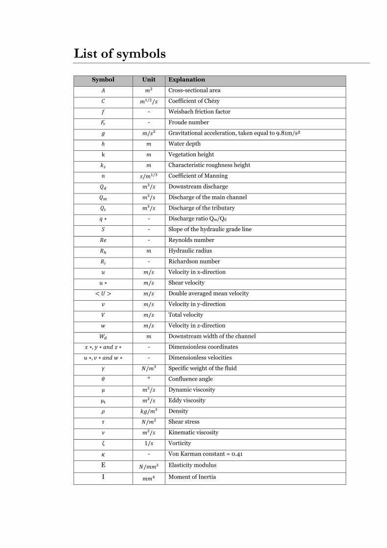
List of symbols

Symbol Unit Explanation

Cross-sectional area

Coefficient of Chézy

- Weisbach friction factor

- Froude number

Gravitational acceleration, taken equal to 9.81m/s²

Water depth

Vegetation height

Characteristic roughness height

Coefficient of Manning

Downstream discharge

Discharge of the main channel

Discharge of the tributary

- Discharge ratio Qm/Qd

- Slope of the hydraulic grade line

- Reynolds number

Hydraulic radius

- Richardson number

Velocity in x-direction

Shear velocity

Double averaged mean velocity

Velocity in y-direction

Total velocity

Velocity in z-direction

Downstream width of the channel

- Dimensionless coordinates

- Dimensionless velocities

Specific weight of the fluid

° Confluence angle

Dynamic viscosity

Eddy viscosity

Density

Shear stress

Kinematic viscosity

Vorticity

- Von Karman constant = 0.41

E Elasticity modulus

I Moment of Inertia

List of abbreviations

Abbreviation Explanation

ADV Acoustic Doppler velocimeter

DCC Direct cross-correlation

FFT Fast Fourier transforms

IA Interrogation area

K-H Kelvin-Helmholtz

LSSPIV Large-scale surface particle image velocimetry

PTV Particle tracking velocimetry

List of figures

Figure 1-1: Components of flow resistance ................................................................................................... 3

Figure 1-2: Moody Diagram for open channels with impervious rigid boundary [Ben Chie Yen (2002)]6

Figure 1-3: Energy cascade [P.A. Davidson (2004)] .................................................................................... 8

Figure 1-4: Boundary layer δ and laminar sublayer ............................................................................... 9

Figure 1-5: Inner and outer law of boundary layer .................................................................................... 10

Figure 1-6: Hydraulically smooth vs. hydraulically rough ......................................................................... 10

Figure 1-7: Channel boundary classification [Ben Chie Yen (2002)] ......................................................... 11

Figure 1-8: Types of rough-surface flows: (a) k-type; (b) d-type; (c) transitional-type [Chow (1959)] .. 12

Figure 1-9: k-type roughness – mechanism [C. Polatel (2006)] ............................................................... 13

Figure 1-10: Possible movements of particles near the bed ....................................................................... 13

Figure 1-11: Forms of bed roughness in sand-bed channels [G.J. Arcement (1989)] .............................. 14

Figure 1-12: Velocity profile - well-submerged vegetation [Galema (2008)] ........................................... 15

Figure 1-13: Velocity profile – submerged vegetation [Galema (2008)] .................................................. 15

Figure 1-14: Three zone sub model [Nezu and Sanjou (2008)] ................................................................. 16

Figure 1-15: Emerged vegetation [Galema (2008)] ................................................................................... 17

Figure 1-16: Energy exchange model – vegetated channels [H.J.S. Fernando (2013)] ........................... 18

Figure 1-17: Effect of submergence depth on Reynolds stresses [Nezu et al. (2008)] ............................. 18

Figure 1-18: Quadrant conditional [Nezu and Nakagawa (1977)] ............................................................. 19

Figure 1-19: Circle C: Sweep – Circle B: Ejection [Nezu and Nakagawa (1977)] ...................................... 19

Figure 1-20: Flexible vegetation compared to rigid vegetation [Carollo et al. (2005)] .......................... 20

Figure 1-21: Flow patterns in dense flexible vegetation. (a) Erect or rigid. (b) Swaying (no organized).

(c) Monami (organized). (d) Prone. [H.J. (2013)] ..................................................................................... 21

Figure 1-22: Subregions of in function of the water depth [Fu-Chun Wu et al. (1999)] .................... 21

Figure 1-23: Composite channel .................................................................................................................. 23

Figure 1-24: Isolines in ducts and open channels (subcritical) - left=smooth/right=rough [Nezu et al.

(1989)] .......................................................................................................................................................... 25

Figure 1-25: Vectorplot in ducts and open channels(subcritical) - left=smooth/right=rough [Nezu et al.

(1989)] .......................................................................................................................................................... 25

Figure 1-26: Classification of secondary currents [Nezu et al. (2005)] .................................................... 26

Figure 1-27: Flow characteristics in an open channel junction [Weber et al. (2001)] ............................. 27

Figure 1-28: Surface velocity pattern (for q*=0.250) from the Iowa experiment [Weber et al. (2001)] 28

Figure 1-29: Schematic of flow structure for q*=0.250 from the Iowa experiment [Shumate (1998)] .. 28

Figure 1-30: Location of the cross-sections and verticals [Weber et al. (2001)] ...................................... 29

Figure 1-31: Secondary flow patterns for q*=0.250: (a) x*=-1.33; (b) x*=-2.00; (c) x*=-5.00, [Shumate

(1998)] .......................................................................................................................................................... 30

Figure 1-32: Diversion flow structure [Barkdoll (2001)] ........................................................................... 30

Figure 1-33: Schematic of flow structure: (a) q*=0.250 en (b) q*=0.750 from the Iowa experiment

[Shumate, 1998] ........................................................................................................................................... 31

Figure 1-34: Water surface mapping for different discharge ratios [Shumate (1998)] ........................... 32

Figure 1-35: Dimensions of the separation zone as a function of the friction coefficient [Creëlle et al.

(2014)] .......................................................................................................................................................... 32

Figure 1-36: Streamlines and water surface mappings for different junction angles [Huang et al.

(2002)] ......................................................................................................................................................... 33

Figure 1-37: Bed discordance (a) 90° Tributary Step; (b) 45° Step Tributary Step [Biron et al. (1996)] 35

Figure 1-38: Principal of flow instability .................................................................................................... 37

Figure 1-39: Location of shear planes at the confluence ........................................................................... 37

Figure 1-40: Kelvin-Helmholtz instability - (a): Situation sketch (b): Initiation of K-H vortex ............. 38

Figure 1-41: Kelvin-Helmholtz instability visible in clouds ....................................................................... 38

Figure 1-42: Curved free shear layer [Liou (1993)] .................................................................................... 39

Figure 1-43: Variation of growth rate α in function of the frequency σ [Liou (1993)] ............................. 40

Figure 1-44: Sketch of the mixing layer in an open channel junction [Mignot et al. (2013)] .................. 41

Figure 1-45: (a) TANH velocity profile; (d) SECH velocity profile; created either by (b)(e) varying

and h = constant or by (c)(f) varying h and = constant [Chu (1991)] .................................................. 43

Figure 1-46: Physical interpretation of Rayleigh’s inflection-point theorem ........................................... 45

Figure 1-47: Velocity and vorticity profiles to demonstrate Fjørtoft criterion ......................................... 45

Figure 2-1: Layout of the test flume ............................................................................................................ 49

Figure 2-2: Filter at inlet channels ............................................................................................................. 50

Figure 2-3: Downstream boundary condition, weir .................................................................................. 50

Figure 2-4: Discharge measurement devices – left: electromagnetic flow meter, right: gauge for the

weir ............................................................................................................................................................... 50

Figure 2-5: Setup of the LSSPIV system ..................................................................................................... 53

Figure 2-6: Principle of LSSPIV – (a): Image recording, (b): First image t=t0, (c): Second image

t=t0+∆t .......................................................................................................................................................... 54

Figure 2-7: LSSPIV coordinate system with the position of the camera .................................................. 55

Figure 2-8: Overlap between subsequent LSSPIV measurements ............................................................ 55

Figure 2-9: Reflection of light during LSSPIV ............................................................................................ 57

Figure 2-10: Close-up of the transmitter and the four beams of the ADV ................................................ 57

Figure 2-11: ADV - positive direction of Bisector (not on scale) ............................................................... 58

Figure 2-12: Measurement range ADV 30-70mm (not on scale) .............................................................. 58

Figure 2-13: Measurement grid - indication of upper boundary of measurement profile ....................... 59

Figure 2-14: Plot of Göring and Nikora Despiking criterion (2002) ........................................................ 60

Figure 2-15: Location of the ADV – cross-sections .................................................................................... 63

Figure 2-16: Inflow section tributary at y*=-1.92 (concrete flume) – Present study ............................... 65

Figure 2-17: Velocity profiles in tributary (y*=-1.92, x*=0.49) – (a): Present study (after), (b): Present

study (before) (c): Schindfessel et al. .......................................................................................................... 66

Figure 2-18: Location grass cover .............................................................................................................. 68

Figure 2-19: Thickness grass cover when compressed by ADV ................................................................ 68

Figure 2-20: Velocity Profile - Sweet spots - Left: Concrete / Right: Grass ............................................. 69

Figure 2-21: Vector plot LSSPIV (concrete) - The dotted line indicates points where u=0..................... 72

Figure 2-22: Vector plot LSSPIV (grass) - The dotted line indicates points where u=0 .......................... 72

Figure 2-23: Contour plot of total velocities (LSSPIV) - left: Concrete / right: Grass ............................. 73

Figure 2-24: Contour plot of the cross-sectional velocities (LSSPIV) - left: Concrete / right: Grass...... 73

Figure 2-25: Cross-section x*=0 – left: Concrete / right: Grass ............................................................... 74

Figure 2-26: Cross-section y*=0 – left: Concrete / right: Grass ............................................................... 74

Figure 2-27: Cross-section x*=-0.5 – left: Concrete / right: Grass ........................................................... 75

Figure 2-28: Cross-section x*=-1.33 – left: Concrete / right: Grass ......................................................... 75

Figure 2-29: Upstream velocities in the recirculation zone – left: concrete / right: grass ...................... 76

Figure 2-30: Velocity Gradient - Mixing layer - Left: Concrete / Right : Grass ....................................... 77

Figure 2-31: Cross-section x*=-0.75 - flume with grass cover ................................................................... 81

Figure 2-32: Cross-section x*=-0.5 - flume with grass cover .................................................................... 81

Figure 2-33: Cross-section x*=-0.25 - flume with grass cover .................................................................. 81

Figure 2-34: Divergence x*=0 - x*=-1.0 - Left: Concrete / Right: Grass ................................................. 83

Figure 2-35: Divergence at separation zone – left: Concrete / right: Grass ............................................ 84

Figure 2-36: Indication of shear planes ...................................................................................................... 85

Figure 2-37: Frame of the existing confluence where the shear planes are visualized with tracers ....... 85

Figure 2-38: Frame of the grass configuration from x*=-0 to x*=-0.66 ................................................. 86

Figure 2-39: Frame of the grass configuration from x*=-1.02 to x*=-1.69 ............................................. 86

Figure 2-40: Frame of the grass configuration from x*=-1.50 to x*=-2.16 ............................................. 86

Figure 2-41: Vorticity - mixing layer – left: concrete / right: grass........................................................... 87

Figure 2-42: Vorticity –Separation zone – Left: Concrete / right: Grass ................................................ 88

List of Tables

Table 1-1: Base values of Manning’s n for natural channels [Arcement et al. (1989)] ............................... 5

Table 1-2: Base values of Manning’s n for artificial channels ..................................................................... 5

Table 1-3: Comparison between present study and the experiments of Shumate (1998) ....................... 29

Table 1-4: Water-surface elevation in function of junction angle θ .......................................................... 34

Table 1-5: Velocity and vorticity profiles to illustrate the Fjørtoft criterion............................................. 46

Table 2-1: Parameters of the experimental setup ...................................................................................... 51

Table 2-2: Locations of the LSSPIV measurements ................................................................................... 56

Table 2-3: Mean and standard deviation of reference measurements - Concrete flume ......................... 62

Table 2-4: Mean and standard deviation of reference measurements - Grass flume .............................. 62

Table 2-5: Location of the ADV – cross-sections ....................................................................................... 63

Table 2-6: Reliability measurements .......................................................................................................... 67

Table 2-7: Location shear layer vs recirculation area ................................................................................ 82

List of Graphs

Graph 2-1: Mean velocities at x*=-1.33 – z=41cm (concrete) ................................................................... 70

Graph 2-2: Standard deviation of the velocities at x*=-1.33 – z=41cm (concrete) .................................. 70

Graph 2-3: Mean velocities at x*=-0.50 (grass) ..........................................................................................71

Graph 2-4: Velocity U1 and U2 - concrete vs grass flume ......................................................................... 78

Graph 2-5: Total Velocity Profile x*=-0.25 - Grass flume ......................................................................... 78

Graph 2-6: ΔU - Concrete vs Grass flume .................................................................................................. 79

Graph 2-7: Maximum Velocity Gradient - Concrete vs Grass flume ........................................................ 79

Graph 2-8: Width δ of the mixing layer - Concrete vs Grass flume ......................................................... 80

Graph 2-9: Total Velocity Profile x*=-1.33 ................................................................................................. 89

1

Introduction

Open channel confluences are frequently encountered in hydraulic structures and in nature

(e.g. a river with a main channel and a lot of tributaries) and form the nodes of the riverine network.

The different flow features often induce important morphodynamic changes that have a significant

effect on the maintenance of these channels. At certain locations sedimentation can occur and other

locations may be affected by scour. Both processes may influence the general flow pattern and alter the

navigability of the confluence.

Despite the fact that a lot of research has been carried out to clarify the flow patterns that occur at a

confluence, the effect of some determining variables is only partially known. On the one hand, the

influence of the geometric characteristics of the channels or the angle at which they meet has already

been investigated. On the other hand, not many studies have been carried out to quantify the influence

of roughness on the flow features at a confluence. In this thesis, experimental research was performed

to clarify some aspects of this influence at a 90° open channel confluence.

Over the past years, a lot of formulas have been derived to describe flow resistance. Some formulas

consider other parameters of the channel in which the fluid flows. Other formulas claim to be more

accurate than some earlier derived equations. Due to all the research that was carried out over the last

decades, it is not clear to see which one is more accurate and where the distinction has to be made

between different situations.

In the following chapter, an attempt will be made to explain some general concepts on roughness and

resistance. After explaining the concept of resistance, the most common equations to express this

resistance will be mentioned. An attempt is made to give some explanation on the resistance in

channels with different roughness. Not all types of surfaces are examined, but the most common

situations are explained. Afterwards, the most important components of a confluence are highlighted

and the possible effect of some variables on the flow pattern will be described. The studies performed

by Shumate et al. (1999) and Schindfessel et al. (2014) are used as a benchmark in the present study.

By comparison with their results, the consistency of the obtained information will be verified.

Furthermore, some general concepts on flow (in)stability will be explained to clarify the occurrence of

instability at the confluence.

With the knowledge of the previous chapter, experimental research is carried out in a test flume at the

Laboratory of Hydraulics in Ghent. Data will be gathered with two different techniques. The main goal

is to verify whether the additional bed roughness influences the flow features at the confluence or not.

With additional measurements the overall result on the flow pattern is estimated and the effect on

different components of the intersection is highlighted. From a comparison of the obtained results

with the data obtained at the concrete set up some distinct changes in flow features are noticed that

partially disagree with some earlier executed studies.

3

1. Literature review

1.1. General concepts

In general, a distinction has to be made between the terms ‘roughness factor’ and ‘resistance

coefficient’. Both terms are not interchangeable, so a clear definition of both words is necessary:

- The resistance coefficient is used to describe and quantify the dynamic behaviour of the

boundary which resists the flow of the fluid. This is expressed in terms of momentum or

energy slopes. This resistance is primarily caused by turbulence developed by surface

properties, geometrical boundaries, obstructions and other factors.

- The roughness factor is a value related to the actual unevenness of the boundary.

In fluid mechanics, hydraulic resistance can be described as the force to overcome the action of the

rigid, flexible or moving boundary on the flow. This can be separated into different components

depending on the writer. In 1964, Leopold et Al. subdivided the resistance into a component due to

skin friction, a component due to internal distortion and one due to spills [1]. Yalin (1977) separated

the resistance into skin roughness, sand wave roughness and resistance due to suspended sediment

[2]. In 1965, Rouse tried to review the hydraulic resistance in open channels [3]. He started by making

a distinction between the following components of flow resistance:

- Surface or skin friction,

- Form resistance or drag,

- Wave resistance from free surface distortion,

- Resistance associated with local accelerations or flow unsteadiness.

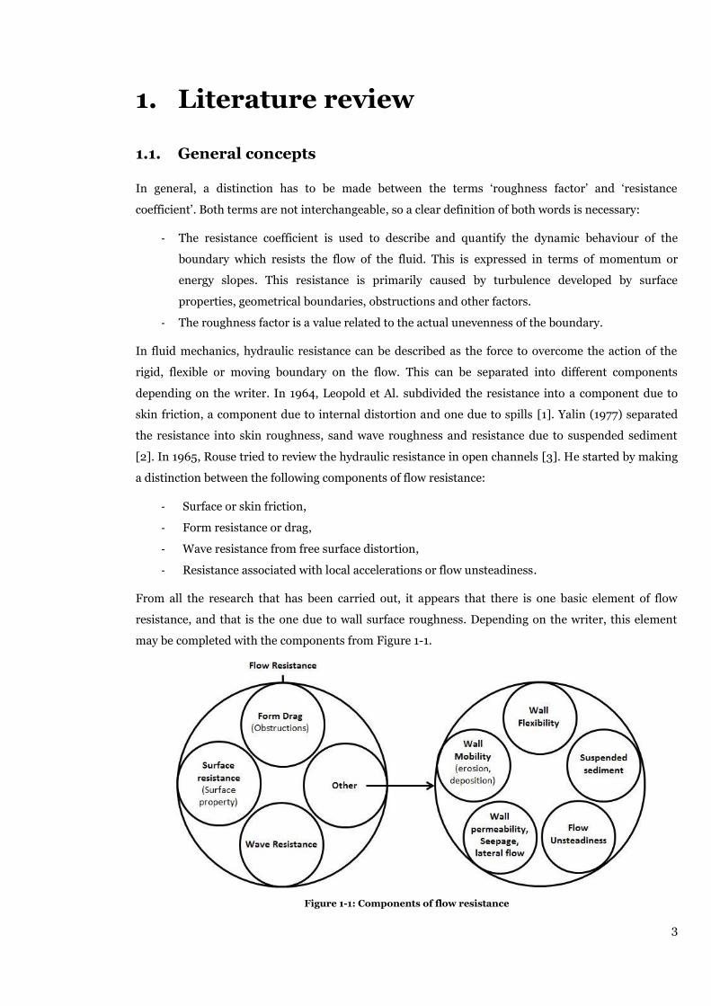
From all the research that has been carried out, it appears that there is one basic element of flow

resistance, and that is the one due to wall surface roughness. Depending on the writer, this element

may be completed with the components from Figure 1-1.

Figure 1-1: Components of flow resistance

4

Form drag resistance occurs as a result of the geometry of the channel. Due to the bending of the river,

the flow has a tendency to form vortices which cause a resistance to the flow. Form drag also occurs

due to elements that are present in the flow (e.g. resistance due to surface geometry, etc.).

In this research, the resistance will be mainly attributed to the surface or skin friction. The test flume

will be equipped with a different bottom type which has another value for the roughness coefficient.

Furthermore, the effects on the flow pattern will be described.

Manning, Weisbach & Chézy coefficients 1.1.1.

The most common used formulas quantifying open channel flow resistance were developed by

Manning, Darcy-Weisbach and Chézy, each relating the cross-sectional velocity U to a certain

coefficient.

-

(Manning)

- √

√ (Darcy-Weisbach)

- √ (Chézy)

With:

- = Hydraulic Radius [m]

- S = Slope of the hydraulic grade line [-]

- √

These coefficients are called the Manning, Weisbach and Chézy coefficients n, f and C and have

different dimensions. These equations can be related to each other by equalizing the velocities in the

previous equations. This makes all three coefficients interchangeable.

√

√

√

√

( 1.1 )

This confirms the presumption that there is not one perfect formula to describe flow resistance and

that a deeper look into the matter is necessary.

From a practical point of view, it is clear that every coefficient has its advantages and disadvantages.

For example, for completely developed turbulent flow over a rigid rough surface, the Manning

coefficient has the advantage of being nearly independent over flow depth h , Reynolds’s number or

the relative roughness

. Chézy is the oldest and most simplified formula and Weisbach’s f is directly

related to the development of fluid mechanics. The disadvantage of Chézy is that no clear table or

figure that lists Chézy coefficients exists.

As the Manning formula is most frequently encountered, this one will be used in practice. To have an

idea on the magnitude of this coefficient, Table 1-1 and Table 1-2 give an overview of the values for

natural channels and artificial channels. Adding some material to the bottom can easily alter these

coefficients so the listed values are only approximately correct.

5

Table 1-1: Base values of Manning’s n for natural channels [Arcement et al. (1989)]

Material Median

size [mm]

n- channel

straight/uniform smooth

Sand

0.2 0.012 -

0.3 0.017 -

0.4 0.02 -

0.5 0.022 -

0.6 0.023 -

0.8 0.025 -

1.0 0.026 -

Concrete - 0.012-0.018 0.011

Rock Cut - - 0.025

Firm Soil - 0.025-0.032 0.200

Coarse Sand 1.0 tot 2.0 0.026-0.035 -

Fine Gravel - - 0.240

Gravel 2 tot 64 0.028-0.035 -

Coarse Gravel - - 0.260

Cobble 64-256 0.030-0.050 -

Boulder >256 0.040-0.070 -

Table 1-2: Base values of Manning’s n for artificial channels

Channel Surface n

Asbestos cement 0.011

Asphalt 0.016

Brick 0.015

Cast-iron 0.012

Concrete 0.012

Copper 0.011

Masonry 0.025

Metal – corrugated 0.016

Glass 0.010

Plastic 0.009

Lead 0.011

Wood 0.012

6

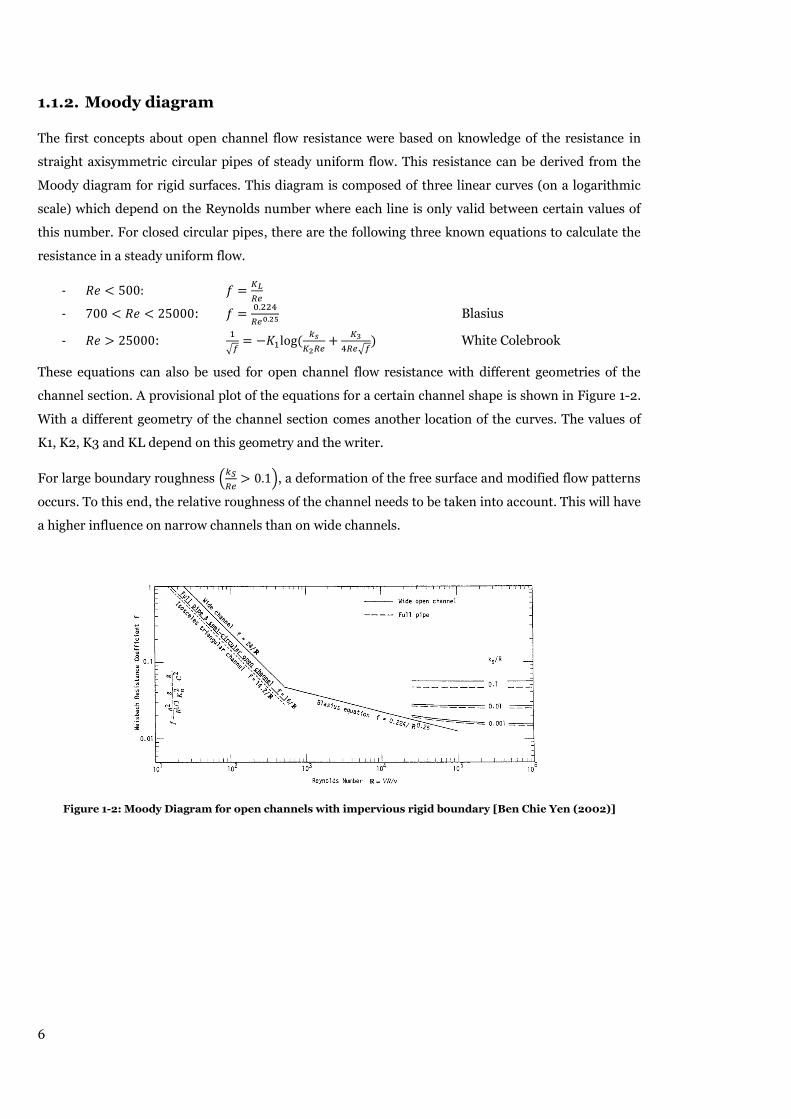
Moody diagram 1.1.2.

The first concepts about open channel flow resistance were based on knowledge of the resistance in

straight axisymmetric circular pipes of steady uniform flow. This resistance can be derived from the

Moody diagram for rigid surfaces. This diagram is composed of three linear curves (on a logarithmic

scale) which depend on the Reynolds number where each line is only valid between certain values of

this number. For closed circular pipes, there are the following three known equations to calculate the

resistance in a steady uniform flow.

-

- :

Blasius

- :

√

√ White Colebrook

These equations can also be used for open channel flow resistance with different geometries of the

channel section. A provisional plot of the equations for a certain channel shape is shown in Figure 1-2.

With a different geometry of the channel section comes another location of the curves. The values of

K1, K2, K3 and KL depend on this geometry and the writer.

For large boundary roughness (

), a deformation of the free surface and modified flow patterns

occurs. To this end, the relative roughness of the channel needs to be taken into account. This will have

a higher influence on narrow channels than on wide channels.

Figure 1-2: Moody Diagram for open channels with impervious rigid boundary [Ben Chie Yen (2002)]

7

Momentum vs energy resistance coefficients 1.1.3.

In §1.1.2, the flow resistance was expressed in function of the energy slope S as is often done in open

channels. With this parameter, flow resistance can be reviewed in two ways. The momentum concept

considers the resistance as the resultant of the forces against a flow. This flow acts on the boundary of

a control volume. The momentum slope then results from external forces that are working on the

boundary of the control volume and is not directly related to the flow inside the control volume/cross-

section. The slope of the momentum resistance along the direction of a channel cross-section is

expressed as:

∫

( 1.2 )

With:

- = specific weight of the fluid

- σ = surface of the boundary

- A = flow cross-sectional area normal to direction bounded by σ

- = directional normal of σ along

- (

)

= shear stress acting on σ

- = turbulence fluctuation with respect to the local mean velocity component

In this approach, the wall surface resistance is reviewed by using the boundary layer theory and the

velocity distribution which will be clarified later. Another way of considering the flow resistance is by

using the energy concept. The energy slope is the energy lost as the fluid moves across the boundary

and can be expressed as:

∫

( 1.3 )

This actually represents the work done by the flow against internal forces. These forces are created by

molecular viscosity and eddy viscosity which overcomes the flow velocity gradient.

Both approaches differ a lot. The energy slope is a scalar quantity while the momentum slope is a

vector quantity. Furthermore, momentum slope resistance is a surface integral or a line integral while

the energy slope resistance is an area integral or a volume integral. So both terms cannot be mixed up.

The exception is steady uniform flow in a straight prismatic channel with a rigid impervious wall and

without lateral flow. Here the channel slope, so both methods lead to the same value

for the resistance. Based on the previous approaches, also the Weisbach, Manning and Chézy

coefficients can be expressed by using these concepts as , in case of the energy concept and

in case of the momentum concept.

In general it is almost impossible to obtain accurate information on the momentum and energy

resistance coefficients except for uniform flow in pipes or 2D channels where the Moody diagram is

available. So the formulas above are not frequently used, but the concepts remain important.

8

Energy Dissipation 1.1.4.

The main question in this paragraph will be: “What happens with the energy?”. When the flow moves

across the channel, it has a certain kinetic energy and a certain velocity. But due to the surface

roughness, the obstacles in the flow, etc., this energy is dissipated and transformed into heat.

At certain locations in the flow, depending on the characteristics of the channel, the flow passes

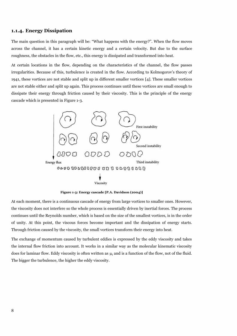
irregularities. Because of this, turbulence is created in the flow. According to Kolmogorov’s theory of

1941, these vortices are not stable and split up in different smaller vortices [4]. These smaller vortices

are not stable either and split up again. This process continues until these vortices are small enough to

dissipate their energy through friction caused by their viscosity. This is the principle of the energy

cascade which is presented in Figure 1-3.

Figure 1-3: Energy cascade [P.A. Davidson (2004)]

At each moment, there is a continuous cascade of energy from large vortices to smaller ones. However,

the viscosity does not interfere so the whole process is essentially driven by inertial forces. The process

continues until the Reynolds number, which is based on the size of the smallest vortices, is in the order

of unity. At this point, the viscous forces become important and the dissipation of energy starts.

Through friction caused by the viscosity, the small vortices transform their energy into heat.

The exchange of momentum caused by turbulent eddies is expressed by the eddy viscosity and takes

the internal flow friction into account. It works in a similar way as the molecular kinematic viscosity

does for laminar flow. Eddy viscosity is often written as and is a function of the flow, not of the fluid.

The bigger the turbulence, the higher the eddy viscosity.

9

1.2. Resistance

Boundary Layer Theory 1.2.1.

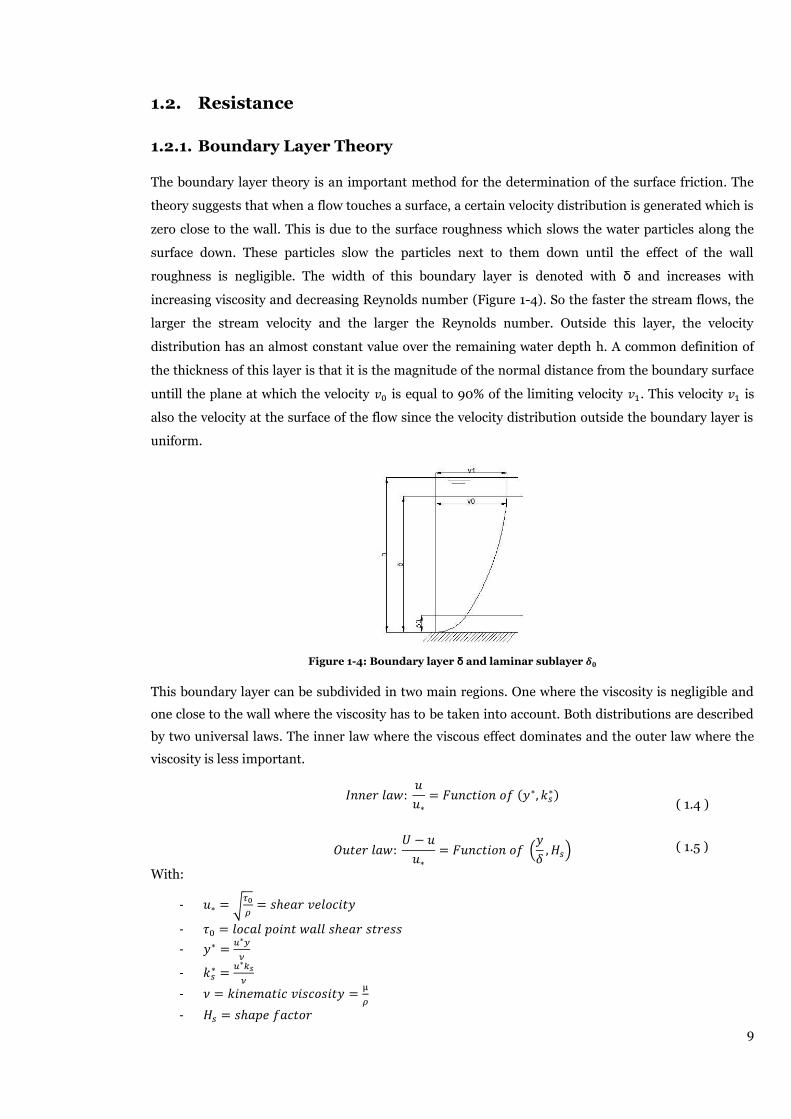
The boundary layer theory is an important method for the determination of the surface friction. The

theory suggests that when a flow touches a surface, a certain velocity distribution is generated which is

zero close to the wall. This is due to the surface roughness which slows the water particles along the

surface down. These particles slow the particles next to them down until the effect of the wall

roughness is negligible. The width of this boundary layer is denoted with δ and increases with

increasing viscosity and decreasing Reynolds number (Figure 1-4). So the faster the stream flows, the

larger the stream velocity and the larger the Reynolds number. Outside this layer, the velocity

distribution has an almost constant value over the remaining water depth h. A common definition of

the thickness of this layer is that it is the magnitude of the normal distance from the boundary surface

untill the plane at which the velocity is equal to 90% of the limiting velocity . This velocity is

also the velocity at the surface of the flow since the velocity distribution outside the boundary layer is

uniform.

Figure 1-4: Boundary layer δ and laminar sublayer

This boundary layer can be subdivided in two main regions. One where the viscosity is negligible and

one close to the wall where the viscosity has to be taken into account. Both distributions are described

by two universal laws. The inner law where the viscous effect dominates and the outer law where the

viscosity is less important.

( 1.4 )

(

) ( 1.5 )

With:

- √

-

-

-

-

-

10

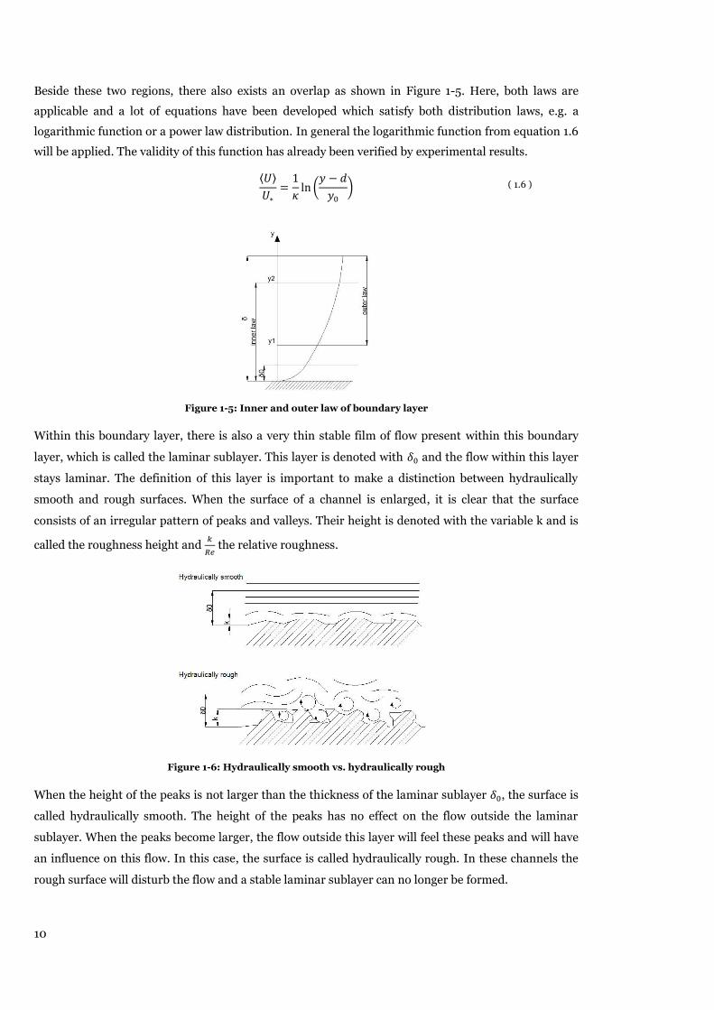
Beside these two regions, there also exists an overlap as shown in Figure 1-5. Here, both laws are

applicable and a lot of equations have been developed which satisfy both distribution laws, e.g. a

logarithmic function or a power law distribution. In general the logarithmic function from equation 1.6

will be applied. The validity of this function has already been verified by experimental results.

⟨ ⟩

(

) ( 1.6 )

Figure 1-5: Inner and outer law of boundary layer

Within this boundary layer, there is also a very thin stable film of flow present within this boundary

layer, which is called the laminar sublayer. This layer is denoted with and the flow within this layer

stays laminar. The definition of this layer is important to make a distinction between hydraulically

smooth and rough surfaces. When the surface of a channel is enlarged, it is clear that the surface

consists of an irregular pattern of peaks and valleys. Their height is denoted with the variable k and is

called the roughness height and

the relative roughness.

Figure 1-6: Hydraulically smooth vs. hydraulically rough

When the height of the peaks is not larger than the thickness of the laminar sublayer , the surface is

called hydraulically smooth. The height of the peaks has no effect on the flow outside the laminar

sublayer. When the peaks become larger, the flow outside this layer will feel these peaks and will have

an influence on this flow. In this case, the surface is called hydraulically rough. In these channels the

rough surface will disturb the flow and a stable laminar sublayer can no longer be formed.

11

The velocity distribution over the boundary layer is related to the flow resistance by using equation 1.7

proposed by Saint-Venant. Stokes (1845) already suggested a similar equation which links the

tangential shear stress to the molecular dynamic viscosity µ and the velocity gradient but this

equation is more general.

(

) ( 1.7 )

With:

-

This equation is applicable to laminar flows when ε equals the dynamic viscosity µ. In this case, the

equation of Stokes equals the proposed equation of Saint-Venant. It can be used to describe turbulent

flow when ε includes the molecular dynamic viscosity and the turbulent viscosity.

The previous explained boundary layer theory gives a clear relation between the velocity distribution

and the shear stress of the wall. However, there are not only rigid impervious surfaces present on the

boundaries of an open channel. Figure 1-7 shows a possible classification of channel boundaries for

steady flows. A different boundary also involves another velocity distribution and another shear stress

on the wall.

Figure 1-7: Channel boundary classification [Ben Chie Yen (2002)]

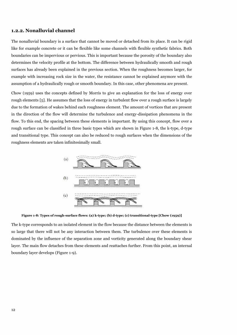
12

Nonalluvial channel 1.2.2.

The nonalluvial boundary is a surface that cannot be moved or detached from its place. It can be rigid

like for example concrete or it can be flexible like some channels with flexible synthetic fabrics. Both

boundaries can be impervious or pervious. This is important because the porosity of the boundary also

determines the velocity profile at the bottom. The difference between hydraulically smooth and rough

surfaces has already been explained in the previous section. When the roughness becomes larger, for

example with increasing rock size in the water, the resistance cannot be explained anymore with the

assumption of a hydraulically rough or smooth boundary. In this case, other phenomena are present.

Chow (1959) uses the concepts defined by Morris to give an explanation for the loss of energy over

rough elements [5]. He assumes that the loss of energy in turbulent flow over a rough surface is largely

due to the formation of wakes behind each roughness element. The amount of vortices that are present

in the direction of the flow will determine the turbulence and energy-dissipation phenomena in the

flow. To this end, the spacing between these elements is important. By using this concept, flow over a

rough surface can be classified in three basic types which are shown in Figure 1-8, the k-type, d-type

and transitional type. This concept can also be reduced to rough surfaces when the dimensions of the

roughness elements are taken infinitesimally small.

Figure 1-8: Types of rough-surface flows: (a) k-type; (b) d-type; (c) transitional-type [Chow (1959)]

The k-type corresponds to an isolated element in the flow because the distance between the elements is

so large that there will not be any interaction between them. The turbulence over these elements is

dominated by the influence of the separation zone and vorticity generated along the boundary shear

layer. The main flow detaches from these elements and reattaches further. From this point, an internal

boundary layer develops (Figure 1-9).

13

Figure 1-9: k-type roughness – mechanism [C. Polatel (2006)]

For the d-type, the elements are so close together that the flow passes the top of the elements. The

holes between the elements contain stable eddies with dead water. The flow will not feel the grooves

and the roughness of the elements, so the surface will be almost hydraulically smooth.

Chow (1959) calls this a quasi-smooth flow. However, a distinction has to be made with hydraulically

smooth surfaces because the eddies in between will still consume a certain amount of energy.

The transitional flow is more difficult. The roughness elements are positioned with a smaller spacing

than k-type roughness but with a larger one than d-type roughness. As a consequence, the wake and

vortex of each element will interfere with those of the following element so a complex interaction takes

place. Here, the height of the elements will be of minor importance.

Alluvial channels 1.2.3.

Alluvial channels have a surface that can be moved due to the flow. The sediment particles have the

ability to be set in motion. Water can then move through the voids between the particles of the bed.

These sediments can cause resistance to the flow because the water puts energy in the movement of

these particles. The latter can occur by rolling or saltation (Figure 1-10).

Figure 1-10: Possible movements of particles near the bed

The resistance of alluvial channels can be split up in two parts. A plane bed that has no geometrical

elements on the bed and a bed form part. The bed form can consist of four important forms. The plane

bed resistance is almost similar to a rigid channel because the source of the resistance is again surface

resistance. However, there are two differences. Firstly, the water has to spend energy in alluvial

channels on rolling and picking up of particles. Secondly the flow, contrary to an impervious boundary,

will move through the voids between the particles. So the boundary is not impermeable. When the

velocity increases or the depth of the flow decreases, the Froude number increases and ripples can be

formed. The sources of this resistance are surface resistance and form resistance so an increase in

resistance coefficient can be seen. For channels with dunes and antidunes also wave resistance has to

be taken into account so an extra resistance is generated.

14

Figure 1-11: Forms of bed roughness in sand-bed channels [G.J. Arcement (1989)]

Due to the presence of these bedforms, turbulence will occur between the crests of each dune. The

same principle can be used as in non-alluvial boundaries, only the square-shaped elements are

replaced by dunes, ripples or antidunes. The bed form can change in an unsteady flow so the resistance

of the bed might also change in time.

When the channel is sufficiently wide and the sediment transport is in equilibrium, the resistance

coefficient f can be simplified so it only depends on four independent variables.

(

)

With:

- = representative size measure of sediment

The alluvial channel resistance can be separated, in a linear way, in two parts so that every part only

depends on two or three of the previous variables.

( 1.8 )

With:

-

-

In this way, the problem of determining f with four independent variables is simplified. This

superposition method was also used for the determination of the bed shear .

( 1.9 )

In the nonlinear approaches, the resistance coefficient is kept as a single factor.

15

1.3. Vegetated Channels

Velocity Profiles 1.3.1.

A lot of variation is possible in vegetated channels. It can be submerged or unsubmerged, flexible or

rigid, etc. All these different configurations with their corresponding surface resistance will modify the

velocity profile of the flow. Depending on the height of the vegetation and of the flow, three different

cases can be distinguished: emergent, submerged and well-submerged vegetation.

Flow over well-submerged vegetation occurs when the water depth h is much higher than the

vegetation height k. The velocity of the flow is delayed within the vegetation, but the flow that goes

over the vegetation is not blocked. When the water depth is high enough, the velocity profile becomes

logarithmic as was the case for a non-alluvial boundary. According to Kleinhans (2008) the vegetation

is well submerged when the water depth is a lot higher than five times the vegetation height [6]. The

situation of well-submerged vegetation is shown in Figure 1-12.

( 1.10 )

Figure 1-12: Velocity profile - well-submerged vegetation [Galema (2008)]

When the water depth is less than five times the vegetation height, but still larger than its height, the

vegetation is submerged (Figure 1-13). In this case the logarithmic velocity profile disappears. The flow

begins to feel the vegetation and the following velocity profile occurs:

Figure 1-13: Velocity profile – submerged vegetation [Galema (2008)]

Previous studies claimed that a two zone sub model is valid. In these models, the velocity profile above

the vegetation had a different path than the one in it. Above the vegetation, the well-known

logarithmic distribution is valid. Within the vegetation, an exponential velocity profile is present.

However, Sanjou and Nezu (2008) proved that this model was not valid [7]. Instead, a three zone sub

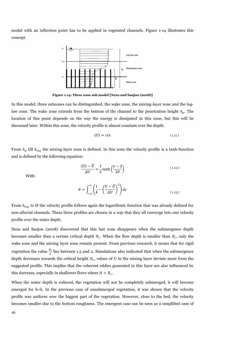
16

model with an inflection point has to be applied in vegetated channels. Figure 1-14 illustrates this

concept.

Figure 1-14: Three zone sub model [Nezu and Sanjou (2008)]

In this model, three subzones can be distinguished, the wake zone, the mixing-layer zone and the log-

law zone. The wake zone extends from the bottom of the channel to the penetration height . The

location of this point depends on the way the energy is dissipated in this zone, but this will be

discussed later. Within this zone, the velocity profile is almost constant over the depth.

⟨ ⟩ ( 1.11 )

From till the mixing-layer zone is defined. In this zone the velocity profile is a tanh-function

and is defined by the following equation:

⟨ ⟩

(

) ( 1.12 )

With:

∫ (

(

)

)

( 1.13 )

From to H the velocity profile follows again the logarithmic function that was already defined for

non-alluvial channels. These three profiles are chosen in a way that they all converge into one velocity

profile over the water depth.

Nezu and Sanjou (2008) discovered that this last zone disappears when the submergence depth

becomes smaller than a certain critical depth . When the flow depth is smaller than , only the

wake zone and the mixing layer zone remain present. From previous research, it seems that for rigid

vegetation the value

lies between 1.5 and 2. Simulations also indicated that when the submergence

depth decreases towards the critical height , values of U in the mixing layer deviate more from the

suggested profile. This implies that the coherent eddies generated in this layer are also influenced by

this decrease, especially in shallower flows where .

When the water depth is reduced, the vegetation will not be completely submerged, it will become

emerged for h<k. In the previous case of unsubmerged vegetation, it was shown that the velocity

profile was uniform over the biggest part of the vegetation. However, close to the bed, the velocity

becomes smaller due to the bottom roughness. The emergent case can be seen as a simplified case of

17

the unsubmerged vegetation. The water flow over the vegetation is diminished so only the flow

through the vegetation remains. From the previous part, it can be seen that the most efficient way to

describe the flow resistance in vegetated channels is by investigating the submerged case.

Figure 1-15: Emerged vegetation [Galema (2008)]

Energy exchange 1.3.2.

By investigating the energy dissipation in the submerged case, a decent explanation for the velocity

profile can be obtained. The part below the penetration depth is called the wake zone. The reason

for this name is that the turbulent transport in this zone is mainly due to the strong wake effects

behind the vegetation stems. This means that the Karman vortex appears significantly in the wake

zone and governs the longitudinal transport of momentum. The turbulence created by these stem

wakes scales significantly with the plant morphology, this is an important factor to consider. Nepf and

Vivoni (2000) called this zone the longitudinal exchange zone [8]. The vertical transport of

momentum or energy is negligible in this zone. The latter is comparable to the emergent vegetated

open channel flow. Within this zone, the flow depends on a balance between vegetative drag and the

pressure gradient.

The value of depends on the author, e.g. Nepf and Vivoni (2000) defined it as the depth at which

the Reynolds stress has decayed to 10% of its maximum value. On the other hand, Ghisalberti and

Nepf (2006) said that the value at which has decayed to zero, is the penetration depth [9].

Hence different definitions of this zone remain available. They also pointed out that the value of the

penetration depth changes when the water depth increases but becomes a constant when the critical

water depth is reached. The contribution from the bottom roughness to the total resistance in

vegetated channels is negligible because the viscous stress and the bed drag appear to be almost

negligible compared to the vegetative drag.

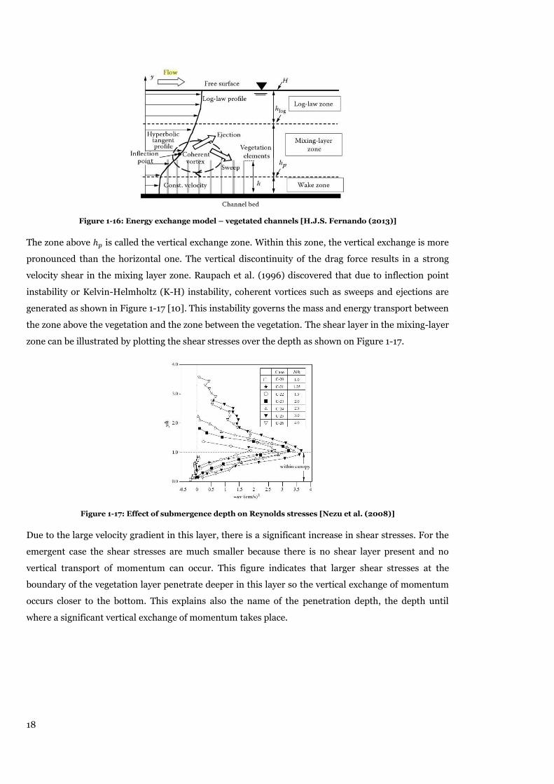
18

Figure 1-16: Energy exchange model – vegetated channels [H.J.S. Fernando (2013)]

The zone above is called the vertical exchange zone. Within this zone, the vertical exchange is more

pronounced than the horizontal one. The vertical discontinuity of the drag force results in a strong

velocity shear in the mixing layer zone. Raupach et al. (1996) discovered that due to inflection point

instability or Kelvin-Helmholtz (K-H) instability, coherent vortices such as sweeps and ejections are

generated as shown in Figure 1-17 [10]. This instability governs the mass and energy transport between

the zone above the vegetation and the zone between the vegetation. The shear layer in the mixing-layer

zone can be illustrated by plotting the shear stresses over the depth as shown on Figure 1-17.

Figure 1-17: Effect of submergence depth on Reynolds stresses [Nezu et al. (2008)]

Due to the large velocity gradient in this layer, there is a significant increase in shear stresses. For the

emergent case the shear stresses are much smaller because there is no shear layer present and no

vertical transport of momentum can occur. This figure indicates that larger shear stresses at the

boundary of the vegetation layer penetrate deeper in this layer so the vertical exchange of momentum

occurs closer to the bottom. This explains also the name of the penetration depth, the depth until

where a significant vertical exchange of momentum takes place.

19

In the mixing layer zone coherent vortices appear due to K-H instability. An explanation for the

exchange of momentum that goes on in these vortices can be given by using the Quadrant Conditional

Analysis of Nakagawa and Nezu (1977) [11]. They made an analysis of the instantaneous Reynolds

stresses. The quadrant Reynolds stress was defined as follows:

∫

( 1.14 )

When u(t) and v(t) exist in a certain quadrant, I(t) equals unity. Otherwise it is zero. Each quadrant

corresponds to a certain event.

- -

-

-

The sum of the Quadrant Reynolds stresses of all quadrants equals unity. These events are illustrated

in Figure 1-18.

Figure 1-18: Quadrant conditional [Nezu and Nakagawa (1977)]

By plotting the contribution of each of these motions over the depth of the flume, a plot similar to

Figure 1-19 can be obtained. This indicates which mechanism is more important than the other over

the depth of the flume. Ejection motions are motions in which low speed fluid is lifted up towards the

free surface and sweep motions are motions in which high speed fluid is inrushed into the vegetation

layer. From simulations, it appeared that both motions occur periodically. Each sweep is followed by

an ejection and these coherent motions are associated with large-scale secondary flows.

Figure 1-19: Circle C: Sweep – Circle B: Ejection [Nezu and Nakagawa (1977)]

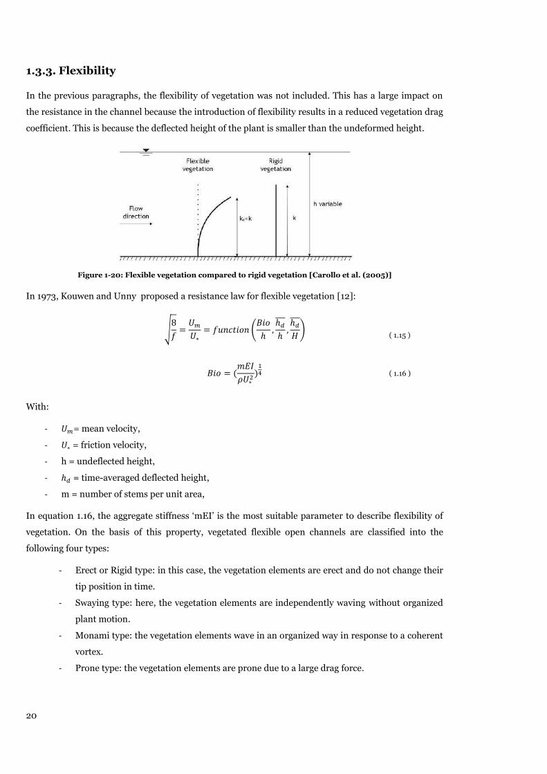
20

Flexibility 1.3.3.

In the previous paragraphs, the flexibility of vegetation was not included. This has a large impact on

the resistance in the channel because the introduction of flexibility results in a reduced vegetation drag

coefficient. This is because the deflected height of the plant is smaller than the undeformed height.

Figure 1-20: Flexible vegetation compared to rigid vegetation [Carollo et al. (2005)]

In 1973, Kouwen and Unny proposed a resistance law for flexible vegetation [12]:

√

(

)

( 1.15 )

( 1.16 )

With:

- = mean velocity,

- = friction velocity,

- h = undeflected height,

- = time-averaged deflected height,

- m = number of stems per unit area,

In equation 1.16, the aggregate stiffness ‘mEI’ is the most suitable parameter to describe flexibility of

vegetation. On the basis of this property, vegetated flexible open channels are classified into the

following four types:

- Erect or Rigid type: in this case, the vegetation elements are erect and do not change their

tip position in time.

- Swaying type: here, the vegetation elements are independently waving without organized

plant motion.

- Monami type: the vegetation elements wave in an organized way in response to a coherent

vortex.

- Prone type: the vegetation elements are prone due to a large drag force.

21

Figure 1-21: Flow patterns in dense flexible vegetation. (a) Erect or rigid. (b) Swaying (no organized). (c)

Monami (organized). (d) Prone. [H.J. (2013)]

The most important one of the previous types is the Monami type. The latter should be distinguished

from the non-organized motion according to Okamoto and Nezu (2009). They pointed out that with

increasing vegetation density, a K-H instability occurs near the vegetation edge and a large-scale

coherent vortex is generated in the mixing layer. For aquatic flexible vegetation, this coherent vortex

will be the cause of the organized plant motion called Monami. Furthermore, due to bending of the

vegetation, the penetration thickness for rigid is larger than for flexible vegetation. As a result, the

transfer of momentum will be less pronounced in the case of flexible vegetation. Wilson et al. (2003)

suggested that the bending of the vegetation surface was the cause of less momentum exchange [13].

The evolution of the resistance coefficient from unsubmerged to submerged vegetation is illustrated in

Figure 1-22. Here, the results of a simplified experimental test that was carried out by Fu-Chun Wu et

al. (1999) is shown [14]. In this analytical model, the flume was covered with separated stems. The

model is a rough approximation so the actual values of the resistance coefficient cannot be applied, but

the evolution of the coefficient stays the same. This is presented in Figure 1-22.

Figure 1-22: Subregions of in function of the water depth [Fu-Chun Wu et al. (1999)]

In the first subregion, the coefficient decreases since the velocity in the flow increases with increasing

depth. In the second subregion, a boundary shear is present from D =0.030 to 0.045 with D the depth

of the flow and T the thickness of the vegetation layer. This boundary shear acts as a resistance to the

free flow over the vegetation so Manning’s n tends to increase. The effect of this layer becomes less

important when the vegetation becomes more submerged so the resistance coefficient decreases again.

This model is only a simplified model but gives a general view on the processes and forces that are

present in submerged and unsubmerged vegetated channels.

23

1.4. Resistance of composite or compound channels

Composite and compound channels are very common in nature. Their roughness coefficient and the

geometric shapes of their cross-sections vary over the entire channel. A composite channel can be

defined as a channel whose wall roughness changes along the wetted perimeter of the cross-section. A

compound channel is a channel that contains different subsections with different geometric shapes.

Usually a compound channel will be a composite channel, e.g. a main channel with floodplains (Figure

1-23). Different subsections and different roughness coefficients are present along this channel.

Figure 1-23: Composite channel

The resistance coefficient of these channels can be expressed by making a weighed sum of the local

resistance coefficient with a weighing function . The cross-sectional value of the resistance

coefficient can then be calculated with the following equation.

∫

( 1.17 )

The fact that the resistance of a composite channel changes across the cross-section also has some

influence on the flow pattern and flow characteristics.

25

1.5. Secondary currents in open channels

Nezu et al. (1989) performed some experiments with regard to the influence of roughness on the

secondary currents in open channels and ducts [15]. Their first discovery was the fact that a dip was

present in the velocity distribution. The maximum velocity appeared to be absent at the free surface

but occurred at a distance of 0.6 times the water height as can be seen on Figure 1-24.

Nezu et al. (1989) proved that the secondary currents were responsible for this phenomenon.

Furthermore, they found that the velocity dip only appeared when the ratio of the channel width to the

water depth was less than five. In this case, the channel was classified as narrow.

Figure 1-24: Isolines in ducts and open channels (subcritical) - left=smooth/right=rough [Nezu et al. (1989)]

The previous figure shows the velocity distribution across half of the channel. It also shows that the

velocity in the rough test flume is more uniformly retarded near the bed. Moreover, the smooth

isolines disappear completely in the rough flume and show a more broken pattern.

Figure 1-25: Vectorplot in ducts and open channels(subcritical) - left=smooth/right=rough [Nezu et al. (1989)]

Figure 1-25 shows vector plots for the smooth and the rough test flume. There exists a strong lateral

component at the free surface in both of them that is directed towards the centre of the channel and is

26

then redirected towards the bottom. Adjacent to this vortex there appears to exist a bottom vortex that

is significantly smaller in size. This vortex is created by the anisotropy of turbulence that is caused by

the free surface effect and the presence of the side wall. With increasing roughness this bottom vortex

disappears while the surface vortex increases in size. These flow characteristics probably will not occur

at the confluence but have to be taken into account when comparing results. The fact that the flow in

one of the branches of the confluence contains a recirculation cell can also slightly be influenced by

these effects.

For curved channels, not only a turbulence-driven force is present but also a centrifugal force. To this

end, a distinction has to be made between the secondary currents that were seen in the straight

channel and the ones encountered in the curved channel. Based on the derivation of the streamwise

component of the channel vorticity, two different types of secondary currents can be described.

Secondary currents in a curved channel are created by the presence of the centrifugal force but also

slightly by the presence of the anisotropic turbulence that was spotted in the straight channel. These

are called secondary currents of the first kind. If the centrifugal force is absent, so the channel is

straight, the currents are from the second kind and the flow characteristics mentioned before are

present. Figure 1-26 points out the differences between both situations.

Figure 1-26: Classification of secondary currents [Nezu et al. (2005)]

27

1.6. Open channels

Open channel confluence 1.6.1.

Open channel confluences are very common in nature where every river consists of a main channel

and some tributaries. Since this is a very important part of the river, it has already led to numerous

studies presented in literature. In this first part, a 90° open channel confluence will be discussed. In

Figure 1-27, the most important flow characteristics of this configuration are shown, with a zone of

separation, a contracted flow region and a shear plane as most important flow regions.

Figure 1-27: Flow characteristics in an open channel junction [Weber et al. (2001)]

The flow features at this junction depend on many geometrical parameters. These include the size and

shape of the channel and also the junction angle. Flow variables such as the Froude number and the

ratio of flow discharge are also of crucial importance. This ratio is defined as:

( 1.18 )

Where and denote the incoming discharge of the main channel and the tributary respectively,

expresses the downstream discharge and is the sum of the discharge of both inlet channels.

The zone of separation is an area just downstream of the tributary, it is a place where the flow has a

small velocity and where recirculation exists. The momentum of the side flow causes the main flow to

detach at the downstream corner of the junction. Studies ([Shumate (1998)], [Best and Reid (1984)])

have shown that the separation zone is significantly longer and wider at the surface level compared to

the bottom of the channel [16] [17]. According to simulations performed by L. Crombé (2013), the

friction coefficient is also a determining parameter [18]. The dimensions of the zone of separation

decreased with increasing roughness. Furthermore, the dimensions of this zone decrease when the

flow ratio q* increases.

The recirculation zone is an area inside the zone of separation where upstream velocities occur. These

velocities decrease towards downstream. Because of the presence of this zone, the water has to pass a

narrower zone. This contracted flow region will have bigger downstream velocities because the same

amount of water has to pass a smaller area.

28

The mixing layer is the area where the fluid of the main channel meets the fluid of the tributary.

Different methods exist to measure and visualize this zone. If different temperatures are assigned to

both flows, the temperature gradient at every location can be seen. This is of course depending on the

flow ratio. Furthermore, the dimensions of the recirculation zone can be determined. Another option is

to give both currents a different concentration of an arbitrary substance. Figure 1-28 shows a surface

velocity plot from the Iowa experiment performed by Shumate (1998). The mixing layer is shown in

the red rectangle. The width of this layer is not constant over the depth of the flume. It decreases in

width from the bottom till the free surface.

Figure 1-28: Surface velocity pattern (for q*=0.250) from the Iowa experiment [Weber et al. (2001)]

Figure 1-29 shows a 3D-configuration of the test setup of the Iowa experiment performed by Shumate.

This 3D-perspective gives more insight in the location and shape of the shear layer and of secondary

currents while a 2D-look focuses more on the general flow patterns of this open channel junction. As

shown in Figure 1-28, the shear plane is not vertical but slightly tilting towards the outer wall.

Figure 1-29: Schematic of flow structure for q*=0.250 from the Iowa experiment [Shumate (1998)]

In the Iowa experiment, measurements were performed at different locations of the flume. The cross-

sections and vertical profiles of these measurements are shown in Figure 1-30. The location of the

cross-sections are dimensionless by dividing the absolute coordinates by the width of the channel

( = 0.914m).

29

Figure 1-30: Location of the cross-sections and verticals [Weber et al. (2001)]

The dimensions of the flume are comparable with the ones of the present study and will give a global

overview of the flow features that can be expected in the present experiment. The most important

characteristics are listed in Table 1-3.

Table 1-3: Comparison between present study and the experiments of Shumate (1998)

Characteristic Present study Shumate (1998)

0.04 0.17

0.104 0.628

0.384 0.271

0.98 0.914

2.36 3.09

0.05 0.37

98000 452000

yes no

In Figure 1-31, vector fields are shown that illustrate the secondary flow patterns in the flume. The flow

at x* = -1.33 (a), just downstream of the channel junction, shows the surface water approaching the

junction-opposite wall (at y* = 1.00). The lateral momentum of the flow is significantly higher near the

surface compared to the bed. Because it is not possible that the flow goes into the wall, the surface flow

is deflected to the bottom. This motion creates a secondary current that is present along the right bank

of the channel (looking downstream). A part of this secondary current, close to the bed, approaches the

junction adjacent wall and is deflected upwards into the zone of separation. This results in a secondary

current further downstream of the confluence (Figure 1-31b). Eventually, at a distance of

approximately 4.00 m downstream, the two secondary currents converge in one large clockwise

rotating current (Figure 1-31c).

30

Figure 1-31: Secondary flow patterns for q*=0.250: (a) x*=-1.33; (b) x*=-2.00; (c) x*=-5.00, [Shumate (1998)]

Comparison of confluence and diversion flow 1.6.2.

Figure 1-32 is a schematic diagram of the flow characteristics in a 90° diverging open channel flow.

When comparing the confluence and the divergence, comparable flow features are observed. The

interaction between the main and the side channel creates a zone of recirculation in both flow

scenarios, but the location changes. In confluence flow, the recirculation zone appears near the main

channel wall, just downstream of the tributary. In diversion flow, this zone occurs on the inside wall of

the tributary. Although the location of the recirculation zone is different, the physics are similar. In

both cases, this zone is wider near the surface than near the bed.

Figure 1-32: Diversion flow structure [Barkdoll (2001)]

Another similarity between both flows is a surface dividing the main channel flow from the side

channel flow. Previously, the dividing surface in confluence flow was called shear plane due to the fact

that two flows are merging, thereby setting up a shearing action as the flow from both channels is

flowing at different velocities. In diversion flow, the surface is called a dividing stream surface because

it cuts the flow in two, entering the side and main channel.

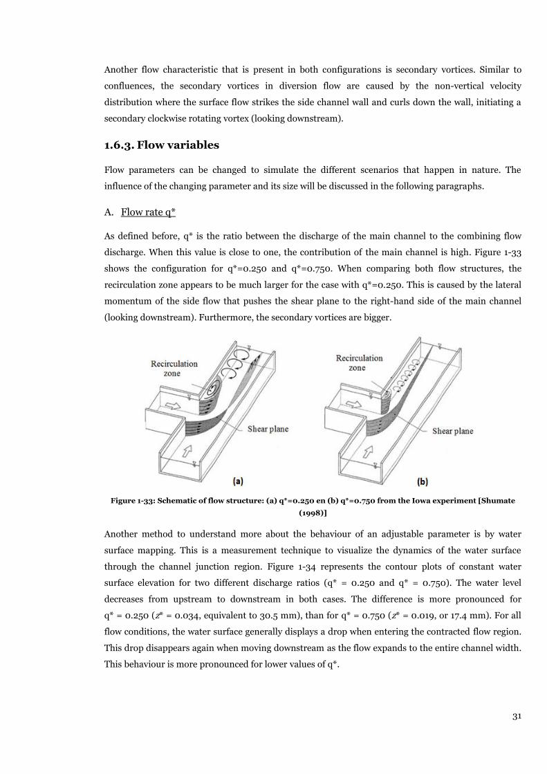
31

Another flow characteristic that is present in both configurations is secondary vortices. Similar to

confluences, the secondary vortices in diversion flow are caused by the non-vertical velocity

distribution where the surface flow strikes the side channel wall and curls down the wall, initiating a

secondary clockwise rotating vortex (looking downstream).

Flow variables 1.6.3.

Flow parameters can be changed to simulate the different scenarios that happen in nature. The

influence of the changing parameter and its size will be discussed in the following paragraphs.

A. Flow rate q*

As defined before, q* is the ratio between the discharge of the main channel to the combining flow

discharge. When this value is close to one, the contribution of the main channel is high. Figure 1-33

shows the configuration for q*=0.250 and q*=0.750. When comparing both flow structures, the

recirculation zone appears to be much larger for the case with q*=0.250. This is caused by the lateral

momentum of the side flow that pushes the shear plane to the right-hand side of the main channel

(looking downstream). Furthermore, the secondary vortices are bigger.

Figure 1-33: Schematic of flow structure: (a) q*=0.250 en (b) q*=0.750 from the Iowa experiment [Shumate

(1998)]

Another method to understand more about the behaviour of an adjustable parameter is by water

surface mapping. This is a measurement technique to visualize the dynamics of the water surface

through the channel junction region. Figure 1-34 represents the contour plots of constant water

surface elevation for two different discharge ratios (q* = 0.250 and q* = 0.750). The water level

decreases from upstream to downstream in both cases. The difference is more pronounced for

q* = 0.250 (z* = 0.034, equivalent to 30.5 mm), than for q* = 0.750 (z* = 0.019, or 17.4 mm). For all

flow conditions, the water surface generally displays a drop when entering the contracted flow region.

This drop disappears again when moving downstream as the flow expands to the entire channel width.

This behaviour is more pronounced for lower values of q*.

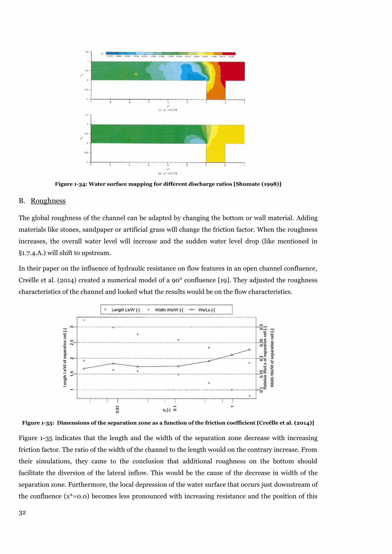
32

Figure 1-34: Water surface mapping for different discharge ratios [Shumate (1998)]

B. Roughness

The global roughness of the channel can be adapted by changing the bottom or wall material. Adding

materials like stones, sandpaper or artificial grass will change the friction factor. When the roughness

increases, the overall water level will increase and the sudden water level drop (like mentioned in

§1.7.4.A.) will shift to upstream.

In their paper on the influence of hydraulic resistance on flow features in an open channel confluence,

Creëlle et al. (2014) created a numerical model of a 90° confluence [19]. They adjusted the roughness

characteristics of the channel and looked what the results would be on the flow characteristics.

Figure 1-35: Dimensions of the separation zone as a function of the friction coefficient [Creëlle et al. (2014)]

Figure 1-35 indicates that the length and the width of the separation zone decrease with increasing

friction factor. The ratio of the width of the channel to the length would on the contrary increase. From

their simulations, they came to the conclusion that additional roughness on the bottom should

facilitate the diversion of the lateral inflow. This would be the cause of the decrease in width of the

separation zone. Furthermore, the local depression of the water surface that occurs just downstream of

the confluence (x*=0.0) becomes less pronounced with increasing resistance and the position of this

33

minimum shifts towards the upstream direction. This corresponds well with the observations of

Shumate (1998).

Furthermore, the simulations showed that the increase of the friction factor at the bottom of the flume

altered the velocity profiles in the different cross-sections. The downstream evolution towards a fully

developed flow seems to occur more easily and the fully developed flow is reached faster.

C. Junction angle

In this paragraph, the influence of the junction angle on the flow characteristics will be discussed.

Huang et al. (1999) made a 3-dimensional numerical study of flows based on the experimental data of

Shumate [20]. He used the data with a low discharge ratio (q*=0.250) because this resulted in a larger

separation zone and a more pronounced water-surface elevation. Figure 1-36 shows the calculated

water-surface elevations and streamlines for four different confluence angles θ.

Figure 1-36: Streamlines and water surface mappings for different junction angles

[Huang et al. (2002)]

One clearly distinguishes that increasing the junction angle leads to higher surface-elevations

upstream of the confluence. The results are listed in Table 1-4. These results are consistent with the

findings of Hsu et al. (1998) who found that the ratio of upstream to downstream depth increases with

increasing junction angle [21].

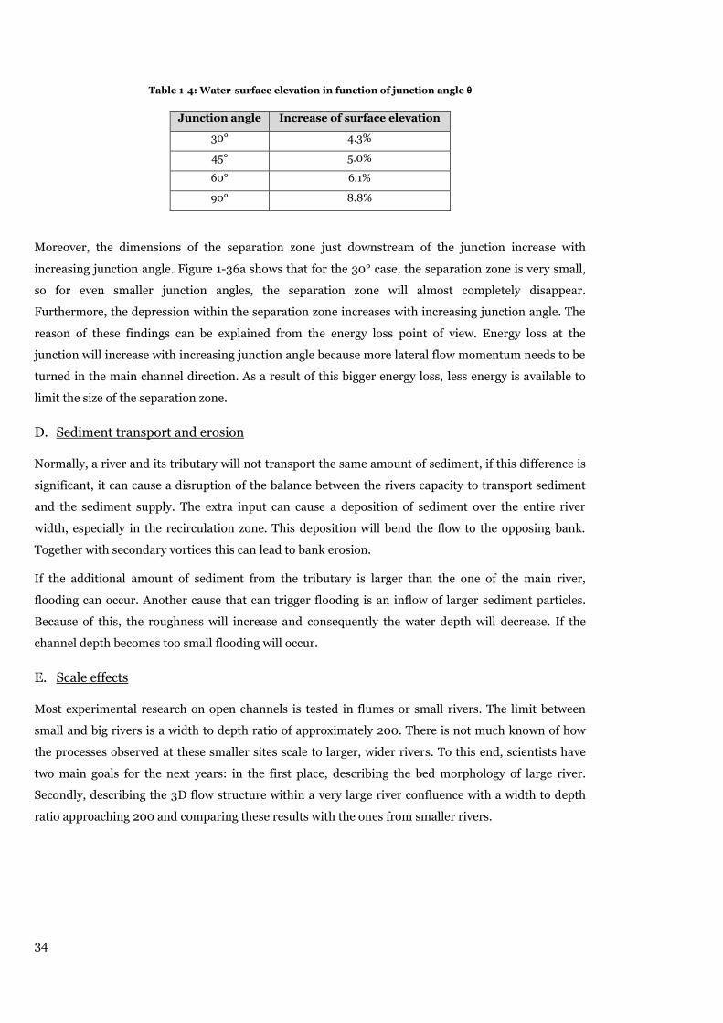
34

Table 1-4: Water-surface elevation in function of junction angle θ

Junction angle Increase of surface elevation

30° 4.3%

45° 5.0%

60° 6.1%

90° 8.8%

Moreover, the dimensions of the separation zone just downstream of the junction increase with

increasing junction angle. Figure 1-36a shows that for the 30° case, the separation zone is very small,

so for even smaller junction angles, the separation zone will almost completely disappear.

Furthermore, the depression within the separation zone increases with increasing junction angle. The

reason of these findings can be explained from the energy loss point of view. Energy loss at the

junction will increase with increasing junction angle because more lateral flow momentum needs to be

turned in the main channel direction. As a result of this bigger energy loss, less energy is available to

limit the size of the separation zone.

D. Sediment transport and erosion

Normally, a river and its tributary will not transport the same amount of sediment, if this difference is

significant, it can cause a disruption of the balance between the rivers capacity to transport sediment

and the sediment supply. The extra input can cause a deposition of sediment over the entire river

width, especially in the recirculation zone. This deposition will bend the flow to the opposing bank.

Together with secondary vortices this can lead to bank erosion.

If the additional amount of sediment from the tributary is larger than the one of the main river,

flooding can occur. Another cause that can trigger flooding is an inflow of larger sediment particles.

Because of this, the roughness will increase and consequently the water depth will decrease. If the

channel depth becomes too small flooding will occur.

E. Scale effects

Most experimental research on open channels is tested in flumes or small rivers. The limit between

small and big rivers is a width to depth ratio of approximately 200. There is not much known of how

the processes observed at these smaller sites scale to larger, wider rivers. To this end, scientists have

two main goals for the next years: in the first place, describing the bed morphology of large river.

Secondly, describing the 3D flow structure within a very large river confluence with a width to depth

ratio approaching 200 and comparing these results with the ones from smaller rivers.

35

F. Bed discordance

Bed discordance between the main and tributary channel is a common phenomenon in most river

confluences, however it is ignored in most models. Biron et al. (1996) used experimental data from a

flume with a junction angle of 30° to investigate this issue. Three different scenarios were investigated

[22]. A situation with concordant beds, one with a 90° tributary step and one with a 45° tributary step.

Those two last scenarios are sketched in Figure 1-37. Their results were focused on four important flow

regions: the zone of separation, the contracted flow region, the zone of deflection and the mixing layer

between both flows.

Figure 1-37: Bed discordance (a) 90° Tributary Step; (b) 45° Step Tributary Step [Biron et al. (1996)]

The experiments pointed out that discordance in bed height between the main channel and tributary

significantly influences the flow dynamics at open channel junctions in three principal ways. At first,

the deflection of the flow from the main channel at the bed may be suppressed. Second, the mixing

layer between the two combining flows is deflected towards the side channel and results in transport of

flow from the deeper main channel into the shallower tributary. Third, water surface differences occur

at the downstream junction corner. In this zone, flow separation is almost absent near the bed,

whereas it is present close to the water surface. The bed height discordance and the presence of a

tributary mouth step results in reduced flow acceleration in the downstream channel. These results

show the importance of bed discordance and it should be taken into account in future models of river

confluence flow dynamics.

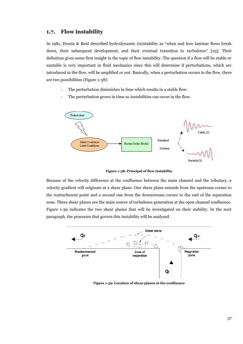
37

1.7. Flow instability

In 1981, Drazin & Reid described hydrodynamic (in)stability as “when and how laminar flows break

down, their subsequent development, and their eventual transition to turbulence” [23]. Their

definition gives some first insight in the topic of flow instability. The question if a flow will be stable or

unstable is very important in fluid mechanics since this will determine if perturbations, which are

introduced in the flow, will be amplified or not. Basically, when a perturbation occurs in the flow, there

are two possibilities (Figure 1-38):

- The perturbation diminishes in time which results in a stable flow.

- The perturbation grows in time so instabilities can occur in the flow.

Figure 1-38: Principal of flow instability

Because of the velocity difference at the confluence between the main channel and the tributary, a

velocity gradient will originate at a shear plane. One shear plane extends from the upstream corner to

the reattachment point and a second one from the downstream corner to the end of the separation

zone. These shear planes are the main source of turbulence generation at the open channel confluence.

Figure 1-39 indicates the two shear planes that will be investigated on their stability. In the next

paragraph, the processes that govern this instability will be analysed.

Figure 1-39: Location of shear planes at the confluence

38

Kelvin-Helmholtz instability 1.7.1.

Kelvin-Helmholtz (K-H) instability is widely known and is generated in density stratified shear flows

or within a single continuous fluid where a shear flow with a strong velocity gradient is present. Two

immiscible and inviscid flows with a different density and velocity are shown in

Figure 1-40a. The lighter fluid, which has the highest velocity, is located above the heavier one. Both

streams interact with each other by a single plane, called the shear plane.

Figure 1-40: Kelvin-Helmholtz instability - (a): Situation sketch (b): Initiation of K-H vortex

The velocity and density profiles of both flows are uniform but the interface between the fluid layers is

discontinuous. This discontinuity in the transverse velocity profile is a shear layer and induces larger

waves in the vicinity of the interface. These waves continue to grow until they turn over and the typical

spiral, which characterizes the Kelvin Helmholtz instability, originates as is indicated in Figure 1-40b.

The breaking waves that generate the mixing are called billows.

An environmental example of this instability is the formation of billow clouds or Kelvin-Helmholtz

clouds. If two different air layers are propagating at a different speed they will form a wave structure.

The top of the fastest cloud layer will try to catch up the slower layer and this results in a rolling

structure (Figure 1-41). Other examples are the air-ocean interface where the density difference is of an

order three, or a river entering a colder lake or a river entering a salty ocean.

Figure 1-41: Kelvin-Helmholtz instability visible in clouds

Instability can be indicated with the Richardson number, Ri. This dimensionless number is the ratio

between the potential and kinetic energy.

(1.19 )

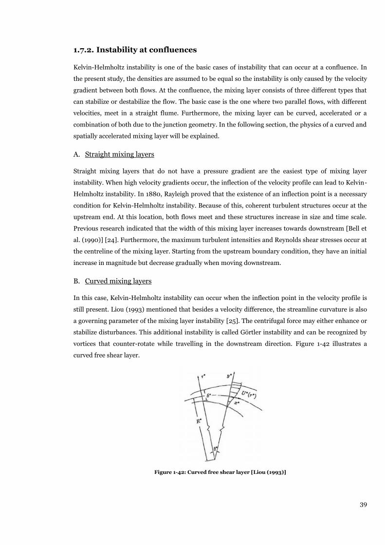
39

Instability at confluences 1.7.2.

Kelvin-Helmholtz instability is one of the basic cases of instability that can occur at a confluence. In

the present study, the densities are assumed to be equal so the instability is only caused by the velocity

gradient between both flows. At the confluence, the mixing layer consists of three different types that

can stabilize or destabilize the flow. The basic case is the one where two parallel flows, with different

velocities, meet in a straight flume. Furthermore, the mixing layer can be curved, accelerated or a

combination of both due to the junction geometry. In the following section, the physics of a curved and

spatially accelerated mixing layer will be explained.

A. Straight mixing layers

Straight mixing layers that do not have a pressure gradient are the easiest type of mixing layer

instability. When high velocity gradients occur, the inflection of the velocity profile can lead to Kelvin-

Helmholtz instability. In 1880, Rayleigh proved that the existence of an inflection point is a necessary

condition for Kelvin-Helmholtz instability. Because of this, coherent turbulent structures occur at the

upstream end. At this location, both flows meet and these structures increase in size and time scale.

Previous research indicated that the width of this mixing layer increases towards downstream [Bell et

al. (1990)] [24]. Furthermore, the maximum turbulent intensities and Reynolds shear stresses occur at

the centreline of the mixing layer. Starting from the upstream boundary condition, they have an initial

increase in magnitude but decrease gradually when moving downstream.

B. Curved mixing layers

In this case, Kelvin-Helmholtz instability can occur when the inflection point in the velocity profile is

still present. Liou (1993) mentioned that besides a velocity difference, the streamline curvature is also

a governing parameter of the mixing layer instability [25]. The centrifugal force may either enhance or

stabilize disturbances. This additional instability is called Görtler instability and can be recognized by

vortices that counter-rotate while travelling in the downstream direction. Figure 1-42 illustrates a

curved free shear layer.

Figure 1-42: Curved free shear layer [Liou (1993)]

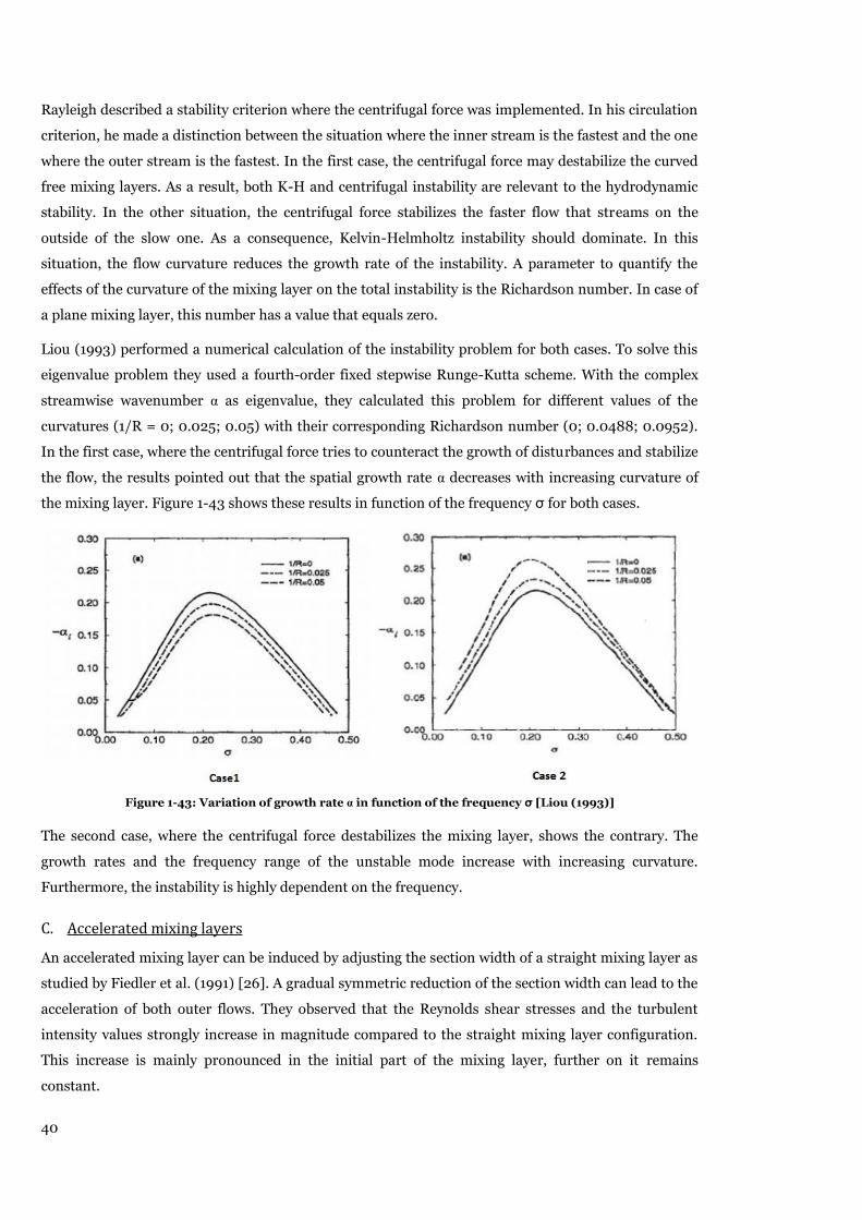
40

Rayleigh described a stability criterion where the centrifugal force was implemented. In his circulation

criterion, he made a distinction between the situation where the inner stream is the fastest and the one

where the outer stream is the fastest. In the first case, the centrifugal force may destabilize the curved

free mixing layers. As a result, both K-H and centrifugal instability are relevant to the hydrodynamic

stability. In the other situation, the centrifugal force stabilizes the faster flow that streams on the

outside of the slow one. As a consequence, Kelvin-Helmholtz instability should dominate. In this

situation, the flow curvature reduces the growth rate of the instability. A parameter to quantify the

effects of the curvature of the mixing layer on the total instability is the Richardson number. In case of

a plane mixing layer, this number has a value that equals zero.

Liou (1993) performed a numerical calculation of the instability problem for both cases. To solve this

eigenvalue problem they used a fourth-order fixed stepwise Runge-Kutta scheme. With the complex

streamwise wavenumber α as eigenvalue, they calculated this problem for different values of the

curvatures (1/R = 0; 0.025; 0.05) with their corresponding Richardson number (0; 0.0488; 0.0952).

In the first case, where the centrifugal force tries to counteract the growth of disturbances and stabilize

the flow, the results pointed out that the spatial growth rate α decreases with increasing curvature of

the mixing layer. Figure 1-43 shows these results in function of the frequency σ for both cases.

Figure 1-43: Variation of growth rate α in function of the frequency σ [Liou (1993)]

The second case, where the centrifugal force destabilizes the mixing layer, shows the contrary. The

growth rates and the frequency range of the unstable mode increase with increasing curvature.

Furthermore, the instability is highly dependent on the frequency.

C. Accelerated mixing layers

An accelerated mixing layer can be induced by adjusting the section width of a straight mixing layer as

studied by Fiedler et al. (1991) [26]. A gradual symmetric reduction of the section width can lead to the

acceleration of both outer flows. They observed that the Reynolds shear stresses and the turbulent

intensity values strongly increase in magnitude compared to the straight mixing layer configuration.

This increase is mainly pronounced in the initial part of the mixing layer, further on it remains

constant.

41

D. Mixing layer in open channel junctions

The mixing layer at a confluence is a combination of the curved and accelerated type. Although these

individual parts are quite straightforward, the application to an open channel junction has some

difficulties. At first, the radius of curvature of the mixing layer is not uniform because it is not

supported by a solid wall. As a result, the shear plane evolves in time and depends on the flow ratio

and the geometric characteristics of the confluence. Secondly, the reduction of the flow section is not

symmetric around the centerline and does not occur gradually.

Figure 1-44: Sketch of the mixing layer in an open channel junction [Mignot et al. (2013)]

42

Influence of a gradient on shear flow stability 1.7.3.

Next to all the previously mentioned parameters that cause instability, the decrease of roughness over

the length of the flume or the immediate increase of the water depth in the flume can cause instability

as investigated by Chu (1991) [27]. His analysis was based on a shallow open channel with a horizontal

length scale significantly larger than the water depth. The Saint-Venant equations were used for the

calculation. His results were correlated with two dimensionless parameters:

- A bed-friction number defined at the inflection point which compares the stabilizing effect of

the bed-friction to the destabilizing effect of the transverse shear.

- A velocity parameter that characterizes the changes in depth and roughness across the open

channel.

In the limiting case of a weak transverse shear flow, the bed-friction number becomes the only

dimensionless parameter governing their stability.

The two most important parameters of the stability of a transverse shear flow are its magnitude and

the degree of bed-friction influence. The bed-friction has a positive and a negative effect on the

stability. On the one hand the bed friction generates small-scale disturbances, but on the other hand, it

has a stabilizing effect on the large-scale transverse disturbances. If this second factor dominates the

process, a transverse shear flow will become stable. Furthermore, a flow can be unstable because of the

inflections in the transverse velocity profile that are produced by the abrupt change in water depth.

Numerical calculations were executed on four groups of parallel flows. The hyperbolic tangent (Tanh)

and the hyperbolic secant velocity profile (Sech) were obtained either by varying the friction coefficient

while keeping the depth h constant or by varying the depth h while keeping the friction coefficient

constant. The obtained velocity profiles are shown in Figure 1-45 and listed below.

- Constant depth and TANH velocity profile

- Constant depth and SECH velocity profile

- Depth-varying flows with uniform bed-friction coefficient

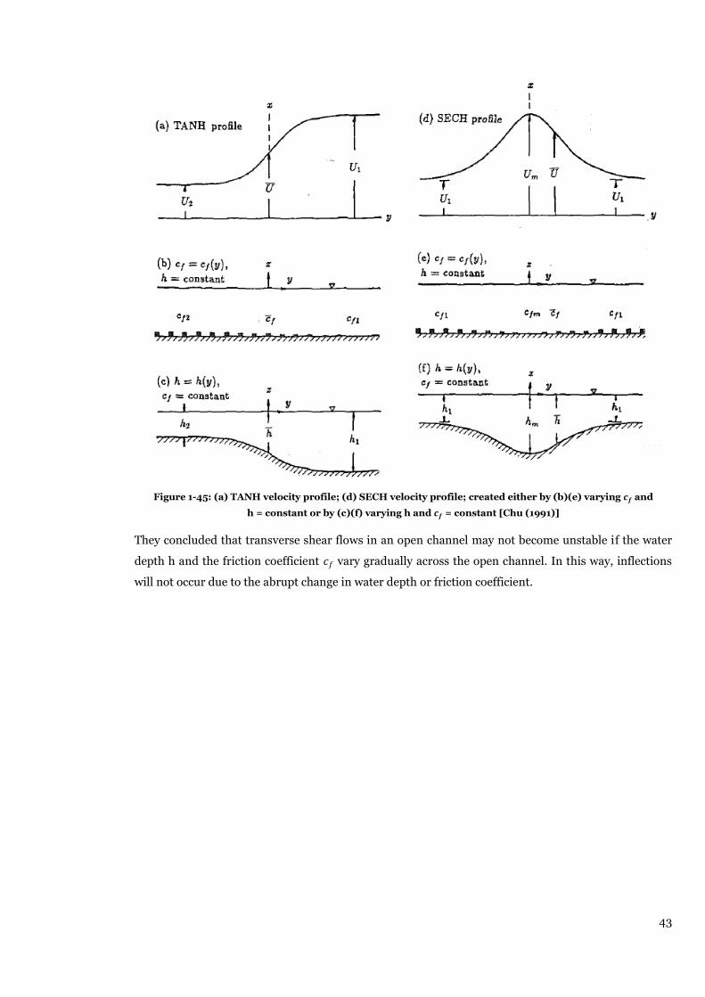
43

Figure 1-45: (a) TANH velocity profile; (d) SECH velocity profile; created either by (b)(e) varying and

h = constant or by (c)(f) varying h and = constant [Chu (1991)]

They concluded that transverse shear flows in an open channel may not become unstable if the water

depth h and the friction coefficient vary gradually across the open channel. In this way, inflections

will not occur due to the abrupt change in water depth or friction coefficient.

44

Shear flow instability criteria 1.7.4.

In the previous paragraphs, a lot of parameters are mentioned that have an influence on the possible

(in)stability of shear planes. In this paragraph, a possible criterion is mentioned to predict whether

instability occurs or not. This criterion will be used in the present study to verify its validity on the

shear planes of the confluence. The occurrence of hydrodynamic instability can be verified by using the

following procedure:

1. Search for a laminar solution to the hydrodynamic equations (Mass conservation and

Navier-Stokes equations) .

2. Add small disturbances to the laminar solution, usually sinusoidal in space and time.

3. Substitute the disturbed solution into the hydrodynamic equations to derive disturbance

equations. This results in an eigenvalue problem for the wave number and frequency of the

disturbances.

4. Solve the eigenvalue problem to study instability.

When following this scheme, three different types of solutions are possible:

- Absolute instabilities where the disturbances grow in time

- Convective instabilities where the disturbances grow in space

- Stable solutions where the disturbances are damped

Orr-Sommerfeld described this eigenvalue problem for viscous parallel flows. Later, Rayleigh (1880)

adapted this equation for inviscous flows and derived a criterion to check the stability of an inviscid

shear flow. This criterion is better known as the Rayleigh’s inflection-point theorem. He verified that

shear flows can be unstable if an inflection point is present in the velocity profile. This condition is

necessary, but not sufficient in order to have inviscid shear flow instability.

The physical interpretation of this theorem will be discussed by introducing the pseudovector

vorticity . This parameter represents a field that describes the local spinning motion of a fluid. For a

two-dimensional shear flow, the vorticity distribution is given by equation 1.20.

( 1.20 )

For the velocity profile shown in Figure 1-46a, the vorticity can be denoted as equation 1.21. When the

velocity field U has an inflection point,

, the vorticity will have a local maximum.

( 1.21 )

Consider a fluid particle that undergoes a virtual displacement from to a region of lower vorticity

(Figure 1-46b). According to the vorticity transport law in an inviscid fluid, this particle takes its

vorticity along with it. As a result, there is a net excess of vorticity which induces a positive vorticial

flow as shown in Figure 1-46c. This rotating current transports lower vorticity from above to the left

http://en.wikipedia.org/wiki/Pseudovector

http://en.wikipedia.org/wiki/Vector_field

http://en.wikipedia.org/wiki/Rotation

http://en.wikipedia.org/wiki/Fluid

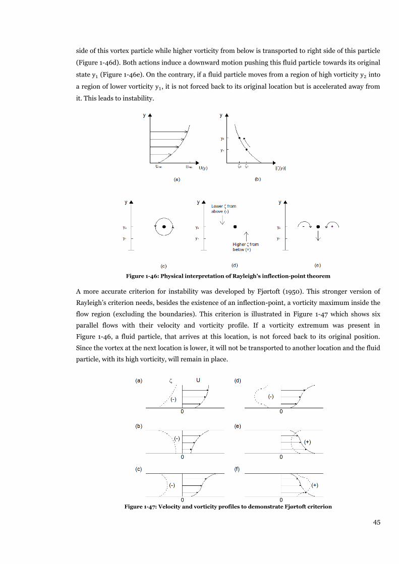
45

side of this vortex particle while higher vorticity from below is transported to right side of this particle

(Figure 1-46d). Both actions induce a downward motion pushing this fluid particle towards its original

state (Figure 1-46e). On the contrary, if a fluid particle moves from a region of high vorticity into

a region of lower vorticity , it is not forced back to its original location but is accelerated away from

it. This leads to instability.

Figure 1-46: Physical interpretation of Rayleigh’s inflection-point theorem

A more accurate criterion for instability was developed by Fjørtoft (1950). This stronger version of

Rayleigh’s criterion needs, besides the existence of an inflection-point, a vorticity maximum inside the

flow region (excluding the boundaries). This criterion is illustrated in Figure 1-47 which shows six

parallel flows with their velocity and vorticity profile. If a vorticity extremum was present in

Figure 1-46, a fluid particle, that arrives at this location, is not forced back to its original position.

Since the vortex at the next location is lower, it will not be transported to another location and the fluid

particle, with its high vorticity, will remain in place.

Figure 1-47: Velocity and vorticity profiles to demonstrate Fjørtoft criterion

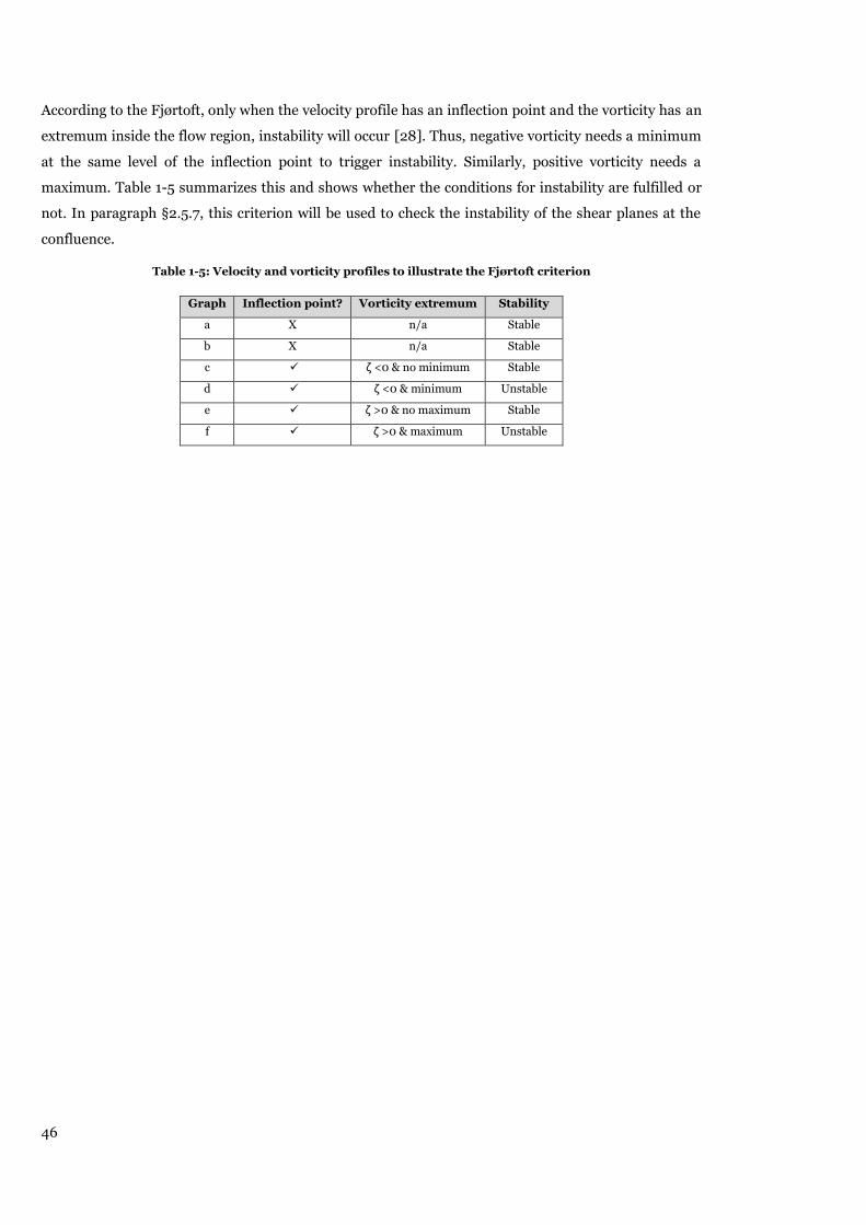
46

According to the Fjørtoft, only when the velocity profile has an inflection point and the vorticity has an

extremum inside the flow region, instability will occur [28]. Thus, negative vorticity needs a minimum

at the same level of the inflection point to trigger instability. Similarly, positive vorticity needs a

maximum. Table 1-5 summarizes this and shows whether the conditions for instability are fulfilled or

not. In paragraph §2.5.7, this criterion will be used to check the instability of the shear planes at the

confluence.

Table 1-5: Velocity and vorticity profiles to illustrate the Fjørtoft criterion

Graph Inflection point? Vorticity extremum Stability

a X n/a Stable

b X n/a Stable

c ζ <0 & no minimum Stable

d ζ <0 & minimum Unstable

e ζ >0 & no maximum Stable

f ζ >0 & maximum Unstable

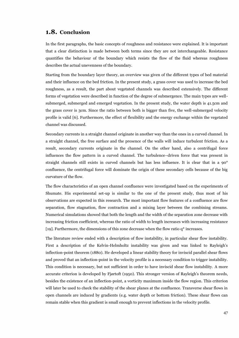
47

1.8. Conclusion

In the first paragraphs, the basic concepts of roughness and resistance were explained. It is important

that a clear distinction is made between both terms since they are not interchangeable. Resistance

quantifies the behaviour of the boundary which resists the flow of the fluid whereas roughness

describes the actual unevenness of the boundary.

Starting from the boundary layer theory, an overview was given of the different types of bed material

and their influence on the bed friction. In the present study, a grass cover was used to increase the bed

roughness, as a result, the part about vegetated channels was described extensively. The different

forms of vegetation were described in function of the degree of submergence. The main types are well-

submerged, submerged and emerged vegetation. In the present study, the water depth is 41.5cm and

the grass cover is 3cm. Since the ratio between both is bigger than five, the well-submerged velocity

profile is valid [6]. Furthermore, the effect of flexibility and the energy exchange within the vegetated

channel was discussed.

Secondary currents in a straight channel originate in another way than the ones in a curved channel. In

a straight channel, the free surface and the presence of the walls will induce turbulent friction. As a

result, secondary currents originate in the channel. On the other hand, also a centrifugal force

influences the flow pattern in a curved channel. The turbulence–driven force that was present in

straight channels still exists in curved channels but has less influence. It is clear that in a 90°

confluence, the centrifugal force will dominate the origin of these secondary cells because of the big

curvature of the flow.

The flow characteristics of an open channel confluence were investigated based on the experiments of

Shumate. His experimental set-up is similar to the one of the present study, thus most of his

observations are expected in this research. The most important flow features of a confluence are flow

separation, flow stagnation, flow contraction and a mixing layer between the combining streams.

Numerical simulations showed that both the length and the width of the separation zone decrease with

increasing friction coefficient, whereas the ratio of width to length increases with increasing resistance

[19]. Furthermore, the dimensions of this zone decrease when the flow ratio q* increases.

The literature review ended with a description of flow instability, in particular shear flow instability.

First a description of the Kelvin-Helmholtz instability was given and was linked to Rayleigh’s

inflection-point theorem (1880). He developed a linear stability theory for inviscid parallel shear flows

and proved that an inflection-point in the velocity profile is a necessary condition to trigger instability.

This condition is necessary, but not sufficient in order to have inviscid shear flow instability. A more

accurate criterion is developed by Fjørtoft (1950). This stronger version of Rayleigh’s theorem needs,

besides the existence of an inflection-point, a vorticity maximum inside the flow region. This criterion

will later be used to check the stability of the shear planes at the confluence. Transverse shear flows in

open channels are induced by gradients (e.g. water depth or bottom friction). These shear flows can

remain stable when this gradient is small enough to prevent inflections in the velocity profile.

49

2. Experiments

2.1. Introduction

In the literature review, the theoretical background of the experimental research was explained. In this

chapter, this information will be used to explain the expected flow features of the experiments and to

interpret the obtained results. At first, the experimental setup with the laboratory flume and the

different measurements devices are explained. Large scale surface particle image velocimetry (LSSPIV)

and measurements with an acoustic Doppler velocimeter (ADV) are performed to obtain experimental

data. The bed material was adjusted to reproduce the effect of changing bed roughness in a confluence.

The basic configuration is the concrete flume while in the second case artificial grass was put on the

bottom to apply another friction factor. Experiments were performed for both configurations with the

same boundary conditions. A constant flow discharge of q*=0.25 was imposed. This value was chosen

based on previous experiments (e.g. Shumate (1998), Schindfessel et al. (2014)) so a comparison can

be made. As mentioned before q* is defined as:

( 2.1 )

Where and denote the incoming discharge of the main channel and the tributary respectively,

expresses the downstream discharge and is the sum of the discharge of both inlet channels.

2.2. Layout of the flume

The experiments were performed at the hydraulics laboratory of Ghent. The open channel facility

consists of a 90° channel confluence with a chamfered rectangular cross-section with concrete walls.

The main channel has a length of 33.18m. The tributary is 5.17m long and intersects with the main

channel at 13.12m (measured from upstream). Both channels have a constant width of 0.98m. The

coordinate system originates at the upstream corner of the junction. The x-axis is orientated along the

main channel towards upstream while the y-axis is pointing in the downstream direction of the

tributary. The coordinates are always represented dimensionless by dividing them by the channel

width . Figure 2-1 gives an overview of the geometrical characteristics of the experimental facility.

Figure 2-1: Layout of the test flume

50

Both inlet channels are connected to the storage tank through pipes. To straighten and stabilize the

flow, filters are installed at the start of both channels. These consist of quarry stones entrapped

between two plates with a honeycomb structure as can be seen on Figure 2-2. As the tributary is only

5.17m long, the flow will probably not be fully developed at the start of the confluence. In the main

channel this is less an issue because its length is 13.16m, so it will be fully developed when it reaches

the confluence. The downstream boundary condition is controlled by a crest weir. Its height is 0.36m

and its width is 0.019m. Some minor leakage is present at both sides of the weir. A picture of the crest

is shown in Figure 2-3.

Figure 2-2: Filter at inlet channels

Figure 2-3: Downstream boundary condition, weir

The flow discharge of the main channel is measured by an electromagnetic flow meter mounted at the

inlet pipe and regulated by an adjustable valve. According to the manufacturer, the accuracy of the

electromagnetic flow meter is . The discharge of the tributary is regulated by a weir that can

be adjusted by a valve. Figure 2-4 shows the discharge measurement devices.

Figure 2-4: Discharge measurement devices – left: electromagnetic flow meter, right: gauge for the weir

51

The downstream discharge of 40 l/s together with a constant downstream water level of 0.415 m

yields to a constant downstream Froude number of 0.05. This number is calculated with equation

2.2 with .

√

( 2.2 )

This value is typical for lowland rivers, (Khublaryan 2009) [29]. The low flow velocities, which are

limited by the robustness of the inlet filter, result in negligible water level differences between the

beginning and the end of the flume. The most important flow parameters are summarized in Table 2-1.

Table 2-1: Parameters of the experimental setup

Flow parameter Value

[m³/s] 0.040

[m/s] 0.104

[m²] 0.384

[m] 0.980

[-] 0.050

[-] 98000

53

2.3. Measurement devices

Large-scale surface particle image velocimetry 2.3.1.

A. Introduction

Large-scale surface particle image velocimetry (LSSPIV) is an optical technique to measure flow

velocities at the free surface. Therefore a 1920x1080 pixel camera is mounted on a horizontal bar and

placed at a fixed height above the water surface taking images at a rate of 15Hz. The setup of the

LSSPIV is shown in Figure 2-5. The fluid is seeded with a tracing material that is recognizable by the

camera. The floating material applied consists of polypropylene particles with a maximum size of

5mm, covered in a white coating. The white coating is used to increase the contrast and makes the

image processing easier. Because the particles are very small, they will not interrupt the average flow

field. This technique results in velocity fields at the free surface.

Figure 2-5: Setup of the LSSPIV system

B. Methodology

The first step in the process is the image recording. The duration of the recording is established on 180

seconds, thus every LSSPIV-measurement captures 2700 frames. This measurement duration results

in a good balance between quality and quantity of the experiments. The obtained frames suffer from

lens distortion but this issue is solved by calibrating them. The processing from frames to velocity data

is done with the freeware PIVlab 1.32. On these frames, the boundary conditions (the walls) have to be

indicated by creating masks on them. When this is done, some pre-processing settings are adjusted to

enhance the results. The next settings can be adapted depending on the resolution and computation

time that is taken as acceptable. Like for every setting, equilibrium needs to be found between the

accuracy of the calculation and the computational time. This was often done by trial and error.

- Contrast-limited adaptive histogram equalization (CLAHE): This setting is enabled by

default and will optimize the contrast of the images and is governed by the size of the

CLAHE filter. With decreasing window size, the contrast will increase but the

computational time will increase as well. A value of 20 pixels seems to give a good balance

between both.

54

- Highpass: When enabled, the images are sharpened and background noise is removed. It

can be adjusted by changing the filter size. In the present, study a value of 25 pixels was

chosen and gave decent results.

- The threshold value for clipping: All values below this threshold are removed, in most

calculations a value of 65 was used.

First, a distinction has to be made between PTV (particle tracking velocimetry) where particle by

particle is followed and PIV (particle image velocimetry) where an area is investigated. In the present

study, PIV is used where a cross-correlation of particles is made. The images are subdivided into

interrogation areas (IA) which contains some particles. The ideal situation is where each IA consists of

a single particle but then it is hard to find this particle back in the second image. Keane and Adrian

(1992) suggest that 8-10 particles within each interrogation area results in the best analysis. An IA is

selected in the first image (Figure 2-6a) and is compared with an area in the second frame [30].

Because the particles have moved over a certain distance D, the area needs to be found in a bigger

searching area (Figure 2-6b). To know the exact displacement of this particle pattern, a cross-

correlation is calculated for all possible displacements within the searching area. Equation 2.3 is used

to calculate the velocity of this area.

( 2.3 )

With:

Figure 2-6: Principle of LSSPIV – (a): Image recording, (b): First image t=t0, (c): Second image t=t0+∆t

PIVlab offers two different LSSPIV algorithms to process the measurements:

- Direct-cross correlation (DCC) where a fixed interrogation area is defined. In this case, the

size of the area and the spacing between different interrogation areas are adjustable.

- FFT window deformation: this algorithm is more accurate because it uses different passes to

arrive at the final interrogation area. First a large interrogation area (e.g. 128 x 64 px) is

chosen. Large areas lead to a better signal-to-noise ratio and a more robust cross correlation.

55

The disadvantage is that it yields a low vector resolution. As a result, the size of the

interrogation area is decreased in the next steps. The writer of the freeware PIVlab

recommends to use three steps because this seems to give an optimal equilibrium between

vector resolution and computation time

In the experiments, the DCC algorithm with an interrogation area of 32 pixels and a step size of 16

pixels was used. This gave decent results and the computation time is smaller than the FFT window

deformation algorithm. After the processing, all velocities are still expressed in pixels/frames. To this

end, a calibration is done to change the velocities from pixel per frame to meter per second. Because of

the fixed height of the camera, a geometrical scale of 1 pixel = 0.00062m is obtained. The y and

z-coordinate of the camera are fixed (y= 0.623m, z=0m) for all measurements, the only geometrical

variable is the x-position of the bar. This is illustrated in Figure 2-7.

Figure 2-7: LSSPIV coordinate system with the position of the camera

With the fixed position of the camera, a rectangle of 0.65 x 1.19m is recorded. To ensure that the whole

area is measured, the borders of the field of view (FOV) between two different measurements need an

overlap. As one measurement covers a length of 0.65m, dx is chosen at 0.5m. In this way, there is an

overlap of 0.15m between two subsequent measurements (Figure 2-8). This overlap is removed in the

post-processing.

Figure 2-8: Overlap between subsequent LSSPIV measurements

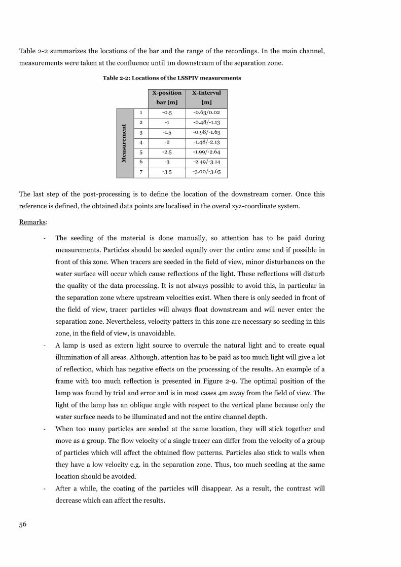
56

Table 2-2 summarizes the locations of the bar and the range of the recordings. In the main channel,

measurements were taken at the confluence until 1m downstream of the separation zone.

Table 2-2: Locations of the LSSPIV measurements

X-position

bar [m]

X-Interval

[m]

Me

as

ur

em

en

t

1 -0.5 -0.63/0.02

2 -1 -0.48/-1.13

3 -1.5 -0.98/-1.63

4 -2 -1.48/-2.13

5 -2.5 -1.99/-2.64

6 -3 -2.49/-3.14

7 -3.5 -3.00/-3.65

The last step of the post-processing is to define the location of the downstream corner. Once this

reference is defined, the obtained data points are localised in the overal xyz-coordinate system.

Remarks:

- The seeding of the material is done manually, so attention has to be paid during

measurements. Particles should be seeded equally over the entire zone and if possible in

front of this zone. When tracers are seeded in the field of view, minor disturbances on the

water surface will occur which cause reflections of the light. These reflections will disturb

the quality of the data processing. It is not always possible to avoid this, in particular in

the separation zone where upstream velocities exist. When there is only seeded in front of

the field of view, tracer particles will always float downstream and will never enter the

separation zone. Nevertheless, velocity patters in this zone are necessary so seeding in this

zone, in the field of view, is unavoidable.

- A lamp is used as extern light source to overrule the natural light and to create equal

illumination of all areas. Although, attention has to be paid as too much light will give a lot

of reflection, which has negative effects on the processing of the results. An example of a

frame with too much reflection is presented in Figure 2-9. The optimal position of the

lamp was found by trial and error and is in most cases 4m away from the field of view. The

light of the lamp has an oblique angle with respect to the vertical plane because only the

water surface needs to be illuminated and not the entire channel depth.

- When too many particles are seeded at the same location, they will stick together and

move as a group. The flow velocity of a single tracer can differ from the velocity of a group

of particles which will affect the obtained flow patterns. Particles also stick to walls when

they have a low velocity e.g. in the separation zone. Thus, too much seeding at the same

location should be avoided.

- After a while, the coating of the particles will disappear. As a result, the contrast will

decrease which can affect the results.

57

Figure 2-9: Reflection of light during LSSPIV

Acoustic Doppler Velocimetry 2.3.2.

A. Methodology

To create velocity a profile in a cross-section of the flume, the ‘Vectrino II Profiling Velocimeter’ is

used. This device is a high-resolution acoustic Doppler velocimeter that can be used to measure

turbulence and velocities in 3D. These velocities are obtained by means of the Doppler effect. The

change of frequency is higher when the acoustic source approaches and lower during the recession.

This change indicates how fast a particle is moving and can be calculated with the following equation:

( 2.4 )

With:

In the present study, the ADV exists of one transmitter and four receivers. The transmitter is located in

the centre of the device and sends out a short pulse. This pulse is reflected on dirt particles that are

suspended in the water and is received by the four beams located at each side of the transmitter as can

be seen on Figure 2-10.

Figure 2-10: Close-up of the transmitter and the four beams of the ADV

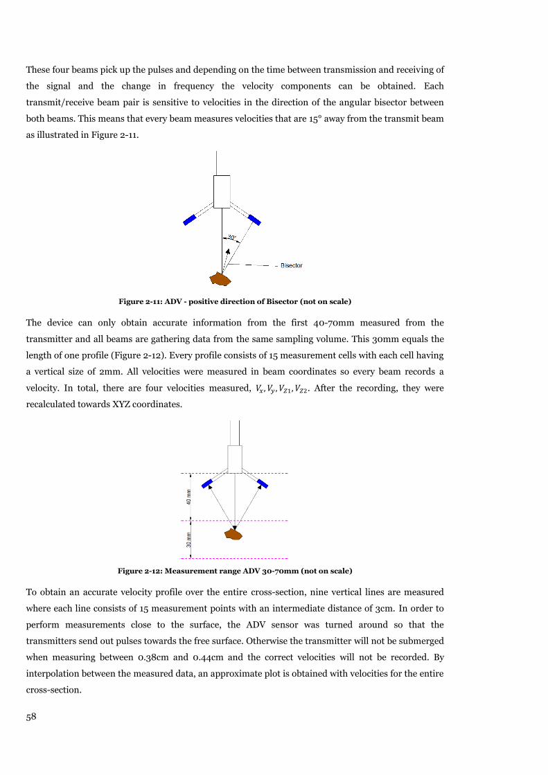
58

These four beams pick up the pulses and depending on the time between transmission and receiving of

the signal and the change in frequency the velocity components can be obtained. Each

transmit/receive beam pair is sensitive to velocities in the direction of the angular bisector between

both beams. This means that every beam measures velocities that are 15° away from the transmit beam

as illustrated in Figure 2-11.

Figure 2-11: ADV - positive direction of Bisector (not on scale)

The device can only obtain accurate information from the first 40-70mm measured from the

transmitter and all beams are gathering data from the same sampling volume. This 30mm equals the

length of one profile (Figure 2-12). Every profile consists of 15 measurement cells with each cell having

a vertical size of 2mm. All velocities were measured in beam coordinates so every beam records a

velocity. In total, there are four velocities measured, . After the recording, they were

recalculated towards XYZ coordinates.

Figure 2-12: Measurement range ADV 30-70mm (not on scale)

To obtain an accurate velocity profile over the entire cross-section, nine vertical lines are measured

where each line consists of 15 measurement points with an intermediate distance of 3cm. In order to

perform measurements close to the surface, the ADV sensor was turned around so that the

transmitters send out pulses towards the free surface. Otherwise the transmitter will not be submerged

when measuring between 0.38cm and 0.44cm and the correct velocities will not be recorded. By

interpolation between the measured data, an approximate plot is obtained with velocities for the entire

cross-section.

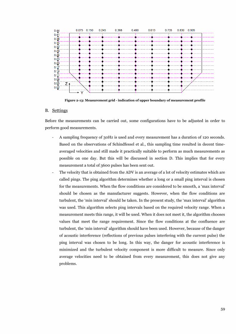
59

Figure 2-13: Measurement grid - indication of upper boundary of measurement profile

B. Settings

Before the measurements can be carried out, some configurations have to be adjusted in order to

perform good measurements.

- A sampling frequency of 30Hz is used and every measurement has a duration of 120 seconds.

Based on the observations of Schindfessel et al., this sampling time resulted in decent time-

averaged velocities and still made it practically suitable to perform as much measurements as

possible on one day. But this will be discussed in section D. This implies that for every

measurement a total of 3600 pulses has been sent out.

- The velocity that is obtained from the ADV is an average of a lot of velocity estimates which are

called pings. The ping algorithm determines whether a long or a small ping interval is chosen

for the measurements. When the flow conditions are considered to be smooth, a ‘max interval’

should be chosen as the manufacturer suggests. However, when the flow conditions are

turbulent, the ‘min interval’ should be taken. In the present study, the ‘max interval’ algorithm

was used. This algorithm selects ping intervals based on the required velocity range. When a

measurement meets this range, it will be used. When it does not meet it, the algorithm chooses

values that meet the range requirement. Since the flow conditions at the confluence are

turbulent, the ‘min interval’ algorithm should have been used. However, because of the danger

of acoustic interference (reflections of previous pulses interfering with the current pulse) the

ping interval was chosen to be long. In this way, the danger for acoustic interference is

minimized and the turbulent velocity component is more difficult to measure. Since only

average velocities need to be obtained from every measurement, this does not give any

problems.

60

- The SNR, signal-to-noise ratio represents the quality of the signal and how large the noise in

the measurement is. If this value is large, the signal will be easy to detect and the amount of

noise will be negligible. If however this ratio is small (<10), the original signal will be very hard

to detect and measures have to be taken to increase this value again. One of the solutions is to

create some suspension in the upstream channels, so more particles become suspended. Low

values of the SNR is the main cause of inaccurate measurements

- The velocity range was always chosen to be 0.5. This gave good results for almost all

measurements. Close to the bottom and in the middle of the cross-section the SNR display

appeared to be stationary at some locations in the profile. It is hypothesized that this is due to

too much reflections at the bottom and due to the geometric characteristics of the cross-

section. This resulted in inaccurate measurements so the velocity range was adjusted towards

values in the range of 0.2-0.4 until the display fluctuated again.

- Also the choice of the location of the measurement profile has to be made. The manufacturer

already suggests a sweet spot exists in the SNR, this spot is located at 5cm below the

transmitter and is the location where the SNR is highest. So the best profiling range is located

around this sweet spot. Because of this, the measurement cell was chosen at 40 to 70mm so

the sweet spot is located in the middle of the profile.

C. Processing

Before the gathered data of the ADV can be used, some post-processing has to be applied. Most of the

time, the ADV does not record the exact 2min so first the records have to be cut off at a duration of 120

seconds.

Figure 2-14: Plot of Göring and Nikora Despiking criterion (2002)

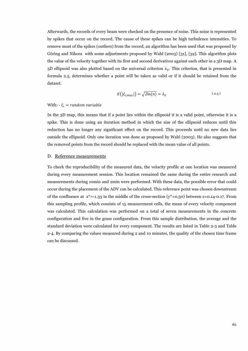
61

Afterwards, the records of every beam were checked on the presence of noise. This noise is represented

by spikes that occur on the record. The cause of these spikes can be high turbulence intensities. To

remove most of the spikes (outliers) from the record, an algorithm has been used that was proposed by

Göring and Nikora with some adjustments proposed by Wahl (2003) [31], [32]. This algorithm plots

the value of the velocity together with its first and second derivatives against each other in a 3D map. A

3D ellipsoid was also plotted based on the universal criterion . This criterion, that is presented in

formula 2.5, determines whether a point will be taken as valid or if it should be retained from the

dataset.

( ) √ ( 2.5 )

With: -

In the 3D map, this means that if a point lies within the ellipsoid it is a valid point, otherwise it is a

spike. This is done using an iteration method in which the size of the ellipsoid reduces until this

reduction has no longer any significant effect on the record. This proceeds until no new data lies

outside the ellipsoid. Only one iteration was done as proposed by Wahl (2003). He also suggests that

the removed points from the record should be replaced with the mean value of all points.

D. Reference measurements

To check the reproducibility of the measured data, the velocity profile at one location was measured

during every measurement session. This location remained the same during the entire research and

measurements during 10min and 2min were performed. With these data, the possible error that could

occur during the placement of the ADV can be calculated. This reference point was chosen downstream

of the confluence at x*=-1.33 in the middle of the cross-section (y*=0.50) between z=0.14-0.17. From

this sampling profile, which consists of 15 measurement cells, the mean of every velocity component

was calculated. This calculation was performed on a total of seven measurements in the concrete

configuration and five in the grass configuration. From this sample distribution, the average and the

standard deviation were calculated for every component. The results are listed in Table 2-3 and Table

2-4. By comparing the values measured during 2 and 10 minutes, the quality of the chosen time frame

can be discussed.

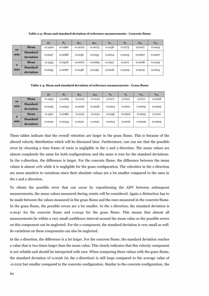
62

Table 2-3: Mean and standard deviation of reference measurements - Concrete flume

10

min

Mean -0.1400 0.0480 -0.0079 -0.0073 0.0156 0.0173 0.0107 0.0103

Standard

deviation 0.0047 0.0086 0.0156 0.0155 0.0014 0.0013 0.0007 0.0007

2

min

Mean -0.1395 0.0476 -0.0070 -0.0063 0.0157 0.0171 0.0108 0.0103

Standard

deviation 0.0055 0.0087 0.0138 0.0136 0.0018 0.0019 0.0015 0.0013

Table 2-4: Mean and standard deviation of reference measurements - Grass flume

10

min

Mean -0.1532 0.0289 -0.0122 -0.0122 0.0171 0.0211 0.0111 0.0108

Standard

deviation 0.0042 0.0034 0.0026 0.0026 0.0013 0.0011 0.0005 0.0005

2

min

Mean -0.1521 0.0282 -0.0121 -0.0121 0.0156 0.0202 0.0103 0.0101

Standard

deviation 0.0019 0.0044 0.0021 0.0021 0.0014 0.0016 0.0009 0.0009

These tables indicate that the overall velocities are larger in the grass flume. This is because of the

altered velocity distribution which will be discussed later. Furthermore, one can see that the possible

error by choosing a time frame of 2min is negligible in the x and y-direction. The mean values are

almost completely the same for both configurations and the same is true for the standard deviations.

In the z-direction, the difference is larger. For the concrete flume, the difference between the mean

values is almost 10% while it is negligible for the grass configuration. The velocities in the z-direction

are more sensitive to variations since their absolute values are a lot smaller compared to the ones in

the x and y-direction.

To obtain the possible error that can occur by repositioning the ADV between subsequent

measurements, the mean values measured during 10min will be considered. Again a distinction has to

be made between the values measured in the grass flume and the ones measured in the concrete flume.

In the grass flume, the possible errors are a lot smaller. In the x-direction, the standard deviation is

0.0047 for the concrete flume and 0.0042 for the grass flume. This means that almost all

measurements lie within a very small confidence interval around the mean value so the possible errors

on this component can be neglected. For the y-component, the standard deviation is very small as well.

So variations on these components can also be neglected.

In the z-direction, the difference is a lot larger. For the concrete flume, the standard deviation reaches

a value that is two times larger than the mean value. This clearly indicates that this velocity component

is not reliable and should be interpreted with care. When comparing these values with the grass flume,

the standard deviation of 0.0026 (in the z-direction) is still large compared to the average value of

-0.0122 but smaller compared to the concrete configuration. Similar to the concrete configuration, the

63

z-component has to be interpreted with care. When both situations are compared, these differences

have to be taken into account. Consistent vertical motions will be reliable and will be present in the

test flume, but individual values will not. The setup of the ADV measurement device is designed so that

the positioning happens as accurately as possible. However, variations are possible since only a visual

control of its perpendicular position was performed. When the comparison is made between the

standard deviations in the concrete and the grass flume, the standard deviations of the samples of the

grass flume are a lot smaller so these data will be much more reliable.

E. Choice cross-sections

To visualize the processes that take place at the confluence, four different cross-sections have been

measured in both situations. These are chosen at x*=0.0, x*=-0.5, x*=-1.33 and y*=0.0 (Figure 2-15).

Figure 2-15: Location of the ADV – cross-sections

The velocities in the cross-section x*=-1.33 give a clear representation of the processes that occur

downstream and the flow features in the separation zone. The cross-section at x*=-0.5 was chosen to

see what processes occur in the confluence before both flows have merged and how the flow from the

tributary responds to the presence of momentum from the main channel. The cross-sections at x*=0.0

and y*=0.0 were chosen so that the inflow of water from both channels could be monitored.

Table 2-5: Location of the ADV – cross-sections

Location ADV – Cross-sections

A = 0

B = 0

C = -0.5

D = -1.33

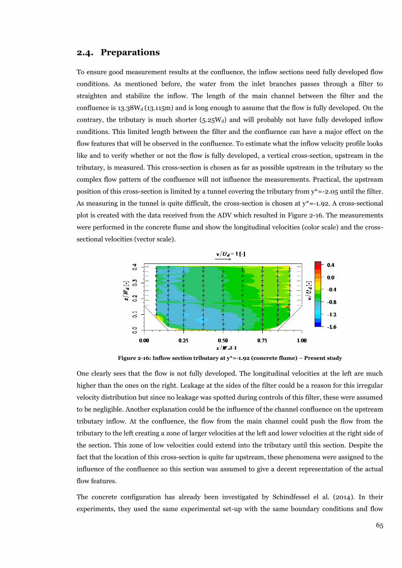
65

2.4. Preparations

To ensure good measurement results at the confluence, the inflow sections need fully developed flow

conditions. As mentioned before, the water from the inlet branches passes through a filter to

straighten and stabilize the inflow. The length of the main channel between the filter and the

confluence is 13.38Wd (13.115m) and is long enough to assume that the flow is fully developed. On the

contrary, the tributary is much shorter (5.25Wd) and will probably not have fully developed inflow

conditions. This limited length between the filter and the confluence can have a major effect on the

flow features that will be observed in the confluence. To estimate what the inflow velocity profile looks

like and to verify whether or not the flow is fully developed, a vertical cross-section, upstream in the

tributary, is measured. This cross-section is chosen as far as possible upstream in the tributary so the

complex flow pattern of the confluence will not influence the measurements. Practical, the upstream

position of this cross-section is limited by a tunnel covering the tributary from y*=-2.05 until the filter.

As measuring in the tunnel is quite difficult, the cross-section is chosen at y*=-1.92. A cross-sectional

plot is created with the data received from the ADV which resulted in Figure 2-16. The measurements

were performed in the concrete flume and show the longitudinal velocities (color scale) and the cross-

sectional velocities (vector scale).

Figure 2-16: Inflow section tributary at y*=-1.92 (concrete flume) – Present study

One clearly sees that the flow is not fully developed. The longitudinal velocities at the left are much

higher than the ones on the right. Leakage at the sides of the filter could be a reason for this irregular

velocity distribution but since no leakage was spotted during controls of this filter, these were assumed

to be negligible. Another explanation could be the influence of the channel confluence on the upstream

tributary inflow. At the confluence, the flow from the main channel could push the flow from the

tributary to the left creating a zone of larger velocities at the left and lower velocities at the right side of

the section. This zone of low velocities could extend into the tributary until this section. Despite the

fact that the location of this cross-section is quite far upstream, these phenomena were assigned to the

influence of the confluence so this section was assumed to give a decent representation of the actual

flow features.

The concrete configuration has already been investigated by Schindfessel el al. (2014). In their

experiments, they used the same experimental set-up with the same boundary conditions and flow

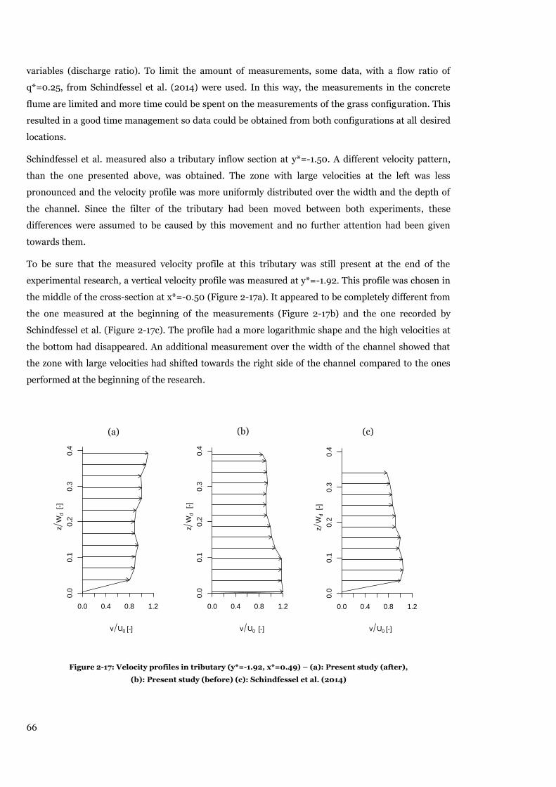
66

variables (discharge ratio). To limit the amount of measurements, some data, with a flow ratio of

q*=0.25, from Schindfessel et al. (2014) were used. In this way, the measurements in the concrete

flume are limited and more time could be spent on the measurements of the grass configuration. This

resulted in a good time management so data could be obtained from both configurations at all desired

locations.

Schindfessel et al. measured also a tributary inflow section at y*=-1.50. A different velocity pattern,

than the one presented above, was obtained. The zone with large velocities at the left was less

pronounced and the velocity profile was more uniformly distributed over the width and the depth of

the channel. Since the filter of the tributary had been moved between both experiments, these

differences were assumed to be caused by this movement and no further attention had been given

towards them.

To be sure that the measured velocity profile at this tributary was still present at the end of the

experimental research, a vertical velocity profile was measured at y*=-1.92. This profile was chosen in

the middle of the cross-section at x*=-0.50 (Figure 2-17a). It appeared to be completely different from

the one measured at the beginning of the measurements (Figure 2-17b) and the one recorded by

Schindfessel et al. (Figure 2-17c). The profile had a more logarithmic shape and the high velocities at

the bottom had disappeared. An additional measurement over the width of the channel showed that

the zone with large velocities had shifted towards the right side of the channel compared to the ones

performed at the beginning of the research.

Figure 2-17: Velocity profiles in tributary (y*=-1.92, x*=0.49) – (a): Present study (after),

(b): Present study (before) (c): Schindfessel et al. (2014)

0.0 0.4 0.8 1.2

0.0

0.1

0.2

0.3

0.4

v U0 [-]

zW

d [-]

0.0 0.4 0.8 1.2

0.0

0.1

0.2

0.3

0.4

v U0 [-]

zW

d [-

]

0.0 0.4 0.8 1.2

0.0

0.1

0.2

0.3

0.4

v U0 [-]

zW

d [-]

(a) (b) (c)

67

No explanation could be given towards these differences since no relocation of the filter had occurred

and during checks of the filter, no leakage problems were discovered. As a consequence, the results in

the following sections have to be handled with care. All three profiles give differences in shape and

magnitude. The velocity profile from Schindfessel et al. showed a good distribution across the width of

the channel. Despite the larger velocities at the bottom, it is assumed that these measurements are

appropriate and that they can be used for comparison with the grass configuration. Since the flow is

uniformly distributed over the width of the channel, changes of this profile at the confluence will be

caused by the confluence and will not have been present at the tributary.

The data gathered for the present study in the concrete flume will not be as reliable as the ones

measured by Schindfessel et al. The large velocity difference between the left and the right side of the

channel may have had a large influence on the flow features at the confluence. As a consequence these

measurements have to be investigated critically. The measurements at the grass configuration are a lot

better. The LSSPIV data shows that the inflow is uniformly distributed over the width of the channel.

Furthermore, the velocity profile shows no large velocities at the bottom. As a consequence, these

measurements are considered to be reliable.

When comparing measurements data, it will always be mentioned who took the measurements so it is

clear which velocity distribution at the tributary was present. At the confluence of the concrete

configuration, almost only the LSSPIV data of Schindfessel et al. was used, so comparisons with

LSSPIV data between concrete and grass will be reliable. Changes in the flow pattern will be caused by

the roughness at the bottom and not by the change in velocity profile at the tributary.

For the ADV-data, the velocity profile at x*=-1.33 at the concrete configuration was measured by

Schindfessel et al. Since the data at the grass configuration is assumed to be reliable, a comparison of

both cross-sections will be reliable. The velocity profile at x*=0 was measured in this research but

since the tributary has no influence on this section these data will be reliable as well. The ADV-data

gathered at the other cross-sections (x*=-0.5 and y*=0) in the concrete configuration has to be studied

critically to draw no false conclusions.

Because the reliability of these inflow sections is important, all measurement data with their

corresponding parameters are summarized in Table 2-6.

Table 2-6: Reliability measurements

Observer Type of bed material Type of measurement reliability results

Schindfessel el al. Concrete All LSSPIV and ADV (x*=-1.33) Good

Present study Concrete ADV (x*=0, x*=-0.5, y*=0) Maybe

Present study Grass All LSSPIV and all ADV Good

In paragraph §2.3.2.D, the reproducibility of the ADV data was checked. The analysis showed that

every measurement session resulted in approximately the same values. The reproducibility of these

data was good which indicates that the flow features at the confluence are less influenced by the

68

different velocity profiles than initially considered. This increases the reliability of the measurements

performed downstream.

The grass cover consists of several parts of different length and width. The location of these elements

was chosen attentive to create a smooth transition between the different grass covers and to minimize

the influence of the flow features at the confluence. The cover indicated with the number three on

Figure 2-18 has a length of 6m and was placed so that the intersection with the cover upstream in the

main channel occurred at approximately x*=1. To this end, the possible influence of this transition on

the confluence will be negligible. This cover extends 5m downstream so the entire investigated part of

the main channel at the confluence is covered with one grass element. In this way, possible changes in

flow features between both ends of the cover are caused by the processes that occur at the confluence

and not by inaccurate placement of the separate elements.

Figure 2-18: Location grass cover

With the placement of the grass cover comes an extra error. The grass cover is approximately 1.1 cm

thick when compressed by the ADV. In the concrete flume, the ADV was standing on top of the

concrete but in the grass flume the device stands on top of the grass cover. Because of this, all values

have to be displaced 1.1 cm upwards. In this way a comparison of both plots is more easily.

Figure 2-19: Thickness grass cover when compressed by ADV

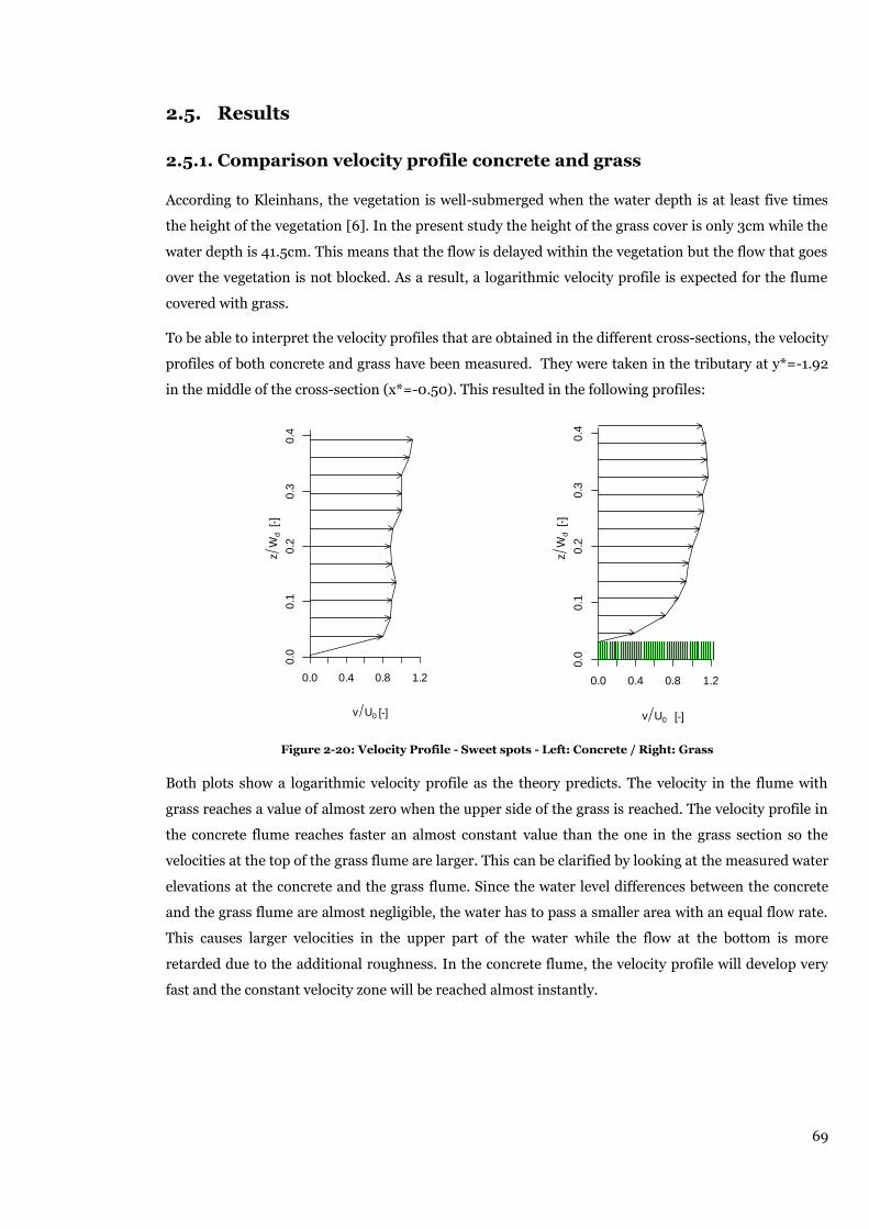
69

2.5. Results

Comparison velocity profile concrete and grass 2.5.1.

According to Kleinhans, the vegetation is well-submerged when the water depth is at least five times

the height of the vegetation [6]. In the present study the height of the grass cover is only 3cm while the

water depth is 41.5cm. This means that the flow is delayed within the vegetation but the flow that goes

over the vegetation is not blocked. As a result, a logarithmic velocity profile is expected for the flume

covered with grass.

To be able to interpret the velocity profiles that are obtained in the different cross-sections, the velocity

profiles of both concrete and grass have been measured. They were taken in the tributary at y*=-1.92

in the middle of the cross-section (x*=-0.50). This resulted in the following profiles:

Figure 2-20: Velocity Profile - Sweet spots - Left: Concrete / Right: Grass

Both plots show a logarithmic velocity profile as the theory predicts. The velocity in the flume with

grass reaches a value of almost zero when the upper side of the grass is reached. The velocity profile in

the concrete flume reaches faster an almost constant value than the one in the grass section so the

velocities at the top of the grass flume are larger. This can be clarified by looking at the measured water

elevations at the concrete and the grass flume. Since the water level differences between the concrete

and the grass flume are almost negligible, the water has to pass a smaller area with an equal flow rate.

This causes larger velocities in the upper part of the water while the flow at the bottom is more

retarded due to the additional roughness. In the concrete flume, the velocity profile will develop very

fast and the constant velocity zone will be reached almost instantly.

0.0 0.4 0.8 1.2

0.0

0.1

0.2

0.3

0.4

v U0 [-]

zW

d [-]

0.0 0.4 0.8 1.2

0.0

0.1

0.2

0.3

0.4

v U0 [-]

zW

d [-]

70

Comparison LSSPIV & ADV 2.5.2.

The methodology of both devices is quite different. However, it is important that both devices give

comparable results at the same location in the flume. Their compatibility will be checked in this

paragraph.

Since the LSSPIV can only measure flow velocities at the surface, the highest measurement row of the

ADV grid will be used to compare with the LSSPIV data. Depending on the cross-section that will be

compared, ADV measurements at z=41cm or z=40cm will be used. This is due to the fact that the ADV

data close to the surface is not always accurate. With an average water depth of 41.5cm, these

measurements will give a decent approximation of the velocities at the water plane. The ADV

measurements were performed at four different cross-sections so a comparison of data at some of

these locations will be made. First the section at x* =-1.33 will be analysed. Graph 2-1 shows the mean

velocities of the concrete configuration measured with both devices.

Graph 2-1: Mean velocities at x*=-1.33 – z=41cm (concrete)

Graph 2-1 indicates that both the magnitude and the shape of the mean velocities give quite similar

results. The location of the separation zone is visible in both measurements and the amplitude of the

velocity gradient is comparable. Graph 2-2 shows the standard deviation of the total velocity V.

Graph 2-2: Standard deviation of the velocities at x*=-1.33 – z=41cm (concrete)

-2

-1.5

-1

-0.5

0

0.5

1

1.5

2

0 0.2 0.4 0.6 0.8 1

Ve

loci

ty /

U0

y/Wd [-]

Vx- LSSPIV Vy- LSSPIV V - LSSPIV

Vx - ADV Vy - ADV V - ADV

0

0.1

0.2

0.3

0.4

0.5

0.6

0 0.2 0.4 0.6 0.8 1

σV

/U

0

y/Wd [-]

σV - ADV σV - LSSPIV

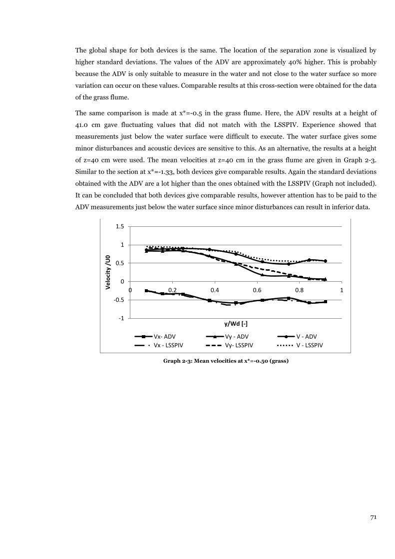
71

The global shape for both devices is the same. The location of the separation zone is visualized by

higher standard deviations. The values of the ADV are approximately 40% higher. This is probably

because the ADV is only suitable to measure in the water and not close to the water surface so more

variation can occur on these values. Comparable results at this cross-section were obtained for the data

of the grass flume.

The same comparison is made at x*=-0.5 in the grass flume. Here, the ADV results at a height of

41.0 cm gave fluctuating values that did not match with the LSSPIV. Experience showed that

measurements just below the water surface were difficult to execute. The water surface gives some

minor disturbances and acoustic devices are sensitive to this. As an alternative, the results at a height

of z=40 cm were used. The mean velocities at z=40 cm in the grass flume are given in Graph 2-3.

Similar to the section at x*=-1.33, both devices give comparable results. Again the standard deviations

obtained with the ADV are a lot higher than the ones obtained with the LSSPIV (Graph not included).

It can be concluded that both devices give comparable results, however attention has to be paid to the

ADV measurements just below the water surface since minor disturbances can result in inferior data.

Graph 2-3: Mean velocities at x*=-0.50 (grass)

-1

-0.5

0

0.5

1

1.5

0 0.2 0.4 0.6 0.8 1Ve

loci

ty /

U0

y/Wd [-]

Vx- ADV Vy - ADV V - ADV

Vx - LSSPIV Vy- LSSPIV V - LSSPIV

72

General flow pattern 2.5.3.

In this paragraph, the general flow pattern together with the main differences between both

configurations will be discussed. This comparison involves LSSPIV data which shows the flow features

at the water surface while the ADV data describes the processes that take place below this surface. The

LSSPIV-data of the concrete flume mainly consists of observations performed by Schindfessel et al.

(2014). Vector plots of the LSSPIV-measurements are shown in Figure 2-21 and Figure 2-22. These

indicate that the presence of the grass cover influences the dimensions of the separation zone. The

length of this zone decreases while the width increases. Inside the separation zone, the flow velocities

at the concrete flume have an upstream directed component. In the other configuration, these

velocities consist of an upstream component together with a lateral one directed towards the

boundaries of the separation zone. Downstream of this zone, this lateral component is still present and

diminishes further downstream. A more extensive description will be discussed in paragraph §2.5.4.

Figure 2-21: Vector plot LSSPIV (concrete) - The dotted line indicates points where u=0

Figure 2-22: Vector plot LSSPIV (grass) - The dotted line indicates points where u=0

73

Figure 2-23 shows contour plots of the surface velocities. In the grass configuration, these are higher

which was also indicated in the velocity profiles of §2.5.1. Because of the larger separation zone, the

flow has to pass a narrower channel so its overall surface velocities increase. At the tributary, the total

velocities are larger for the grass configuration which results in a smaller stagnation zone at the

upstream corner. Furthermore, the plot at the grass configuration indicates that the inflow from the

tributary is more uniformly distributed over the width of the channel.

Figure 2-23: Contour plot of total velocities (LSSPIV) - left: Concrete / right: Grass

Figure 2-24 shows the higher velocities in the cross-sectional-direction at the grass configuration. Due

to the larger velocities in the tributary, the flow enters the confluence with a larger force and pushes

the water from the main channel further to the side.

Figure 2-24: Contour plot of the cross-sectional velocities (LSSPIV) - left: Concrete / right: Grass

Four different cross-sections were measured using the ADV in both configurations and are shown in

the figures below. First the two cross-sections just before the confluence (x*=0 in the main channel

and y*=0 in the tributary) will be discussed. Afterwards, the cross-section at x*=-0.5 and the one

downstream of the confluence (x*=-1.33) will be analysed. Attention has to be paid while analysing the

plots at y*=0 and x*=-0.5 at the concrete configuration since these can be influenced by the changed

velocity profile, as mentioned in §2.4.

The ADV-plots at x*=0 (Figure 2-25) indicate that the highest downstream velocities occur at the wall

opposing the tributary (y*=1). This is due to the flow contraction caused by the lateral momentum of

the tributary. The flow on the left bank is decelerated and ends in the stagnation zone. The cross-

sectional motion, shown as arrows, is quite similar in both configurations. Its distribution is uniform

over the width of the channel and small in magnitude.

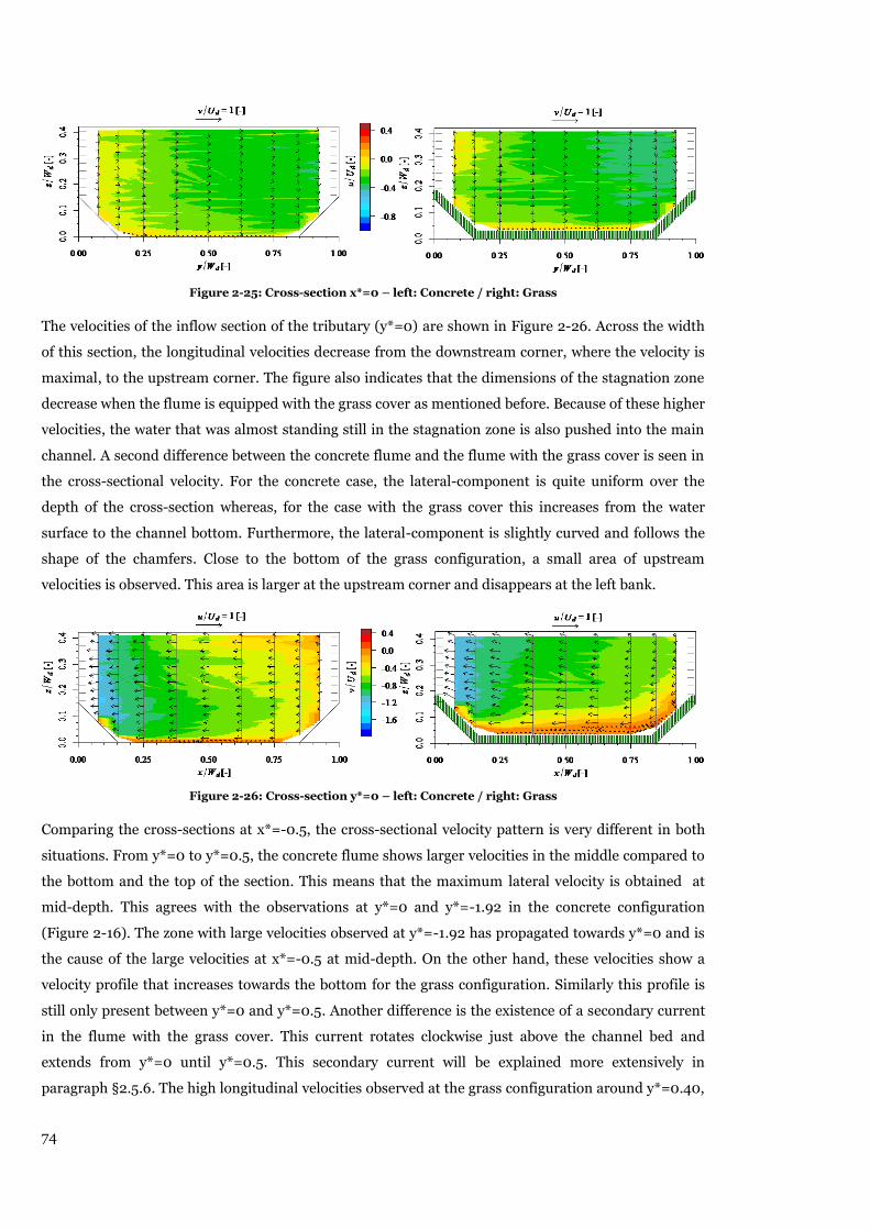
74

Figure 2-25: Cross-section x*=0 – left: Concrete / right: Grass

The velocities of the inflow section of the tributary (y*=0) are shown in Figure 2-26. Across the width

of this section, the longitudinal velocities decrease from the downstream corner, where the velocity is

maximal, to the upstream corner. The figure also indicates that the dimensions of the stagnation zone

decrease when the flume is equipped with the grass cover as mentioned before. Because of these higher

velocities, the water that was almost standing still in the stagnation zone is also pushed into the main

channel. A second difference between the concrete flume and the flume with the grass cover is seen in

the cross-sectional velocity. For the concrete case, the lateral-component is quite uniform over the

depth of the cross-section whereas, for the case with the grass cover this increases from the water

surface to the channel bottom. Furthermore, the lateral-component is slightly curved and follows the

shape of the chamfers. Close to the bottom of the grass configuration, a small area of upstream

velocities is observed. This area is larger at the upstream corner and disappears at the left bank.

Figure 2-26: Cross-section y*=0 – left: Concrete / right: Grass

Comparing the cross-sections at x*=-0.5, the cross-sectional velocity pattern is very different in both

situations. From y*=0 to y*=0.5, the concrete flume shows larger velocities in the middle compared to

the bottom and the top of the section. This means that the maximum lateral velocity is obtained at

mid-depth. This agrees with the observations at y*=0 and y*=-1.92 in the concrete configuration

(Figure 2-16). The zone with large velocities observed at y*=-1.92 has propagated towards y*=0 and is

the cause of the large velocities at x*=-0.5 at mid-depth. On the other hand, these velocities show a

velocity profile that increases towards the bottom for the grass configuration. Similarly this profile is

still only present between y*=0 and y*=0.5. Another difference is the existence of a secondary current

in the flume with the grass cover. This current rotates clockwise just above the channel bed and

extends from y*=0 until y*=0.5. This secondary current will be explained more extensively in

paragraph §2.5.6. The high longitudinal velocities observed at the grass configuration around y*=0.40,

75

indicate the location of the shear plane. The lateral inflow from the tributary is transformed in a

longitudinal component. This results in a reduction of this lateral component around this location.

Figure 2-27: Cross-section x*=-0.5 – left: Concrete / right: Grass

The last cross-section that will be discussed is located downstream of the confluence at x*=-1.33. The

measurement data of the concrete case is based on the experiments of Schindfessel et al. (2014). The

plots of this cross-section are shown in Figure 2-28 and show a clockwise rotating cell in the

separation zone. The dotted contour line indicates points with a longitudinal velocity of zero. Within

this zone, positive (upstream) velocities are present. For both cases the highest upstream velocities in

the separation zone appear at the water surface and decrease in magnitude when moving towards the

bottom. The secondary cell does not extend until the bottom of the flume but stops somewhere in

between.

For the concrete case, the separation zone is constant in width and ends at z*=0.10. This is contrary to

the results of Shumate who predicts a separation zone that decreases in width towards the bottom [16].

These differences are due to the presence of the chamfers. The larger longitudinal velocities near the

bottom of the left bank are caused by the reduced transfer of lateral momentum from the tributary to

the main channel. These observations were already made by Schindfessel el al. (2014).

For the case with the grass cover, the separation zone still extends vertically but ends already at mid-

depth (z*=0.20). Lateral inflow from the tributary collides on the flow of the main channel, bends

downward and is redirected towards the left bank. This is the reason for the abrupt end of the

separation zone at a depth of z*=0.20. This phenomenon does not appear for the concrete case

because here, the lateral velocities are smaller and do not have the power to reach the left bank after

the collision with the stream of the main channel. The zone with large velocities around y*=0.40 has

increased in comparison with the concrete flume. This will be further explained in §2.5.6.

Figure 2-28: Cross-section x*=-1.33 – left: Concrete / right: Grass

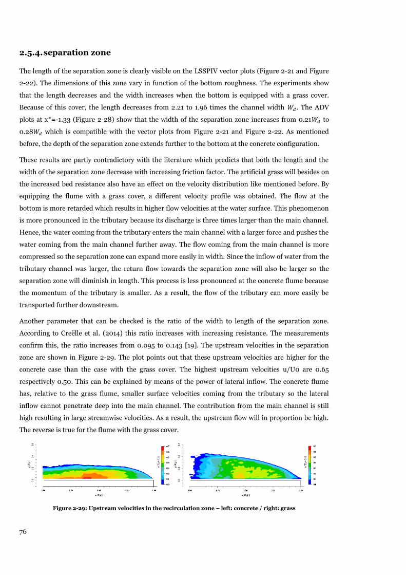
76

separation zone 2.5.4.

The length of the separation zone is clearly visible on the LSSPIV vector plots (Figure 2-21 and Figure

2-22). The dimensions of this zone vary in function of the bottom roughness. The experiments show

that the length decreases and the width increases when the bottom is equipped with a grass cover.

Because of this cover, the length decreases from 2.21 to 1.96 times the channel width . The ADV

plots at x*=-1.33 (Figure 2-28) show that the width of the separation zone increases from 0.21 to

0.28 which is compatible with the vector plots from Figure 2-21 and Figure 2-22. As mentioned

before, the depth of the separation zone extends further to the bottom at the concrete configuration.

These results are partly contradictory with the literature which predicts that both the length and the

width of the separation zone decrease with increasing friction factor. The artificial grass will besides on

the increased bed resistance also have an effect on the velocity distribution like mentioned before. By

equipping the flume with a grass cover, a different velocity profile was obtained. The flow at the

bottom is more retarded which results in higher flow velocities at the water surface. This phenomenon

is more pronounced in the tributary because its discharge is three times larger than the main channel.

Hence, the water coming from the tributary enters the main channel with a larger force and pushes the

water coming from the main channel further away. The flow coming from the main channel is more

compressed so the separation zone can expand more easily in width. Since the inflow of water from the

tributary channel was larger, the return flow towards the separation zone will also be larger so the

separation zone will diminish in length. This process is less pronounced at the concrete flume because

the momentum of the tributary is smaller. As a result, the flow of the tributary can more easily be

transported further downstream.

Another parameter that can be checked is the ratio of the width to length of the separation zone.

According to Creëlle et al. (2014) this ratio increases with increasing resistance. The measurements

confirm this, the ratio increases from 0.095 to 0.143 [19]. The upstream velocities in the separation

zone are shown in Figure 2-29. The plot points out that these upstream velocities are higher for the

concrete case than the case with the grass cover. The highest upstream velocities u/U0 are 0.65

respectively 0.50. This can be explained by means of the power of lateral inflow. The concrete flume

has, relative to the grass flume, smaller surface velocities coming from the tributary so the lateral

inflow cannot penetrate deep into the main channel. The contribution from the main channel is still

high resulting in large streamwise velocities. As a result, the upstream flow will in proportion be high.

The reverse is true for the flume with the grass cover.

Figure 2-29: Upstream velocities in the recirculation zone – left: concrete / right: grass

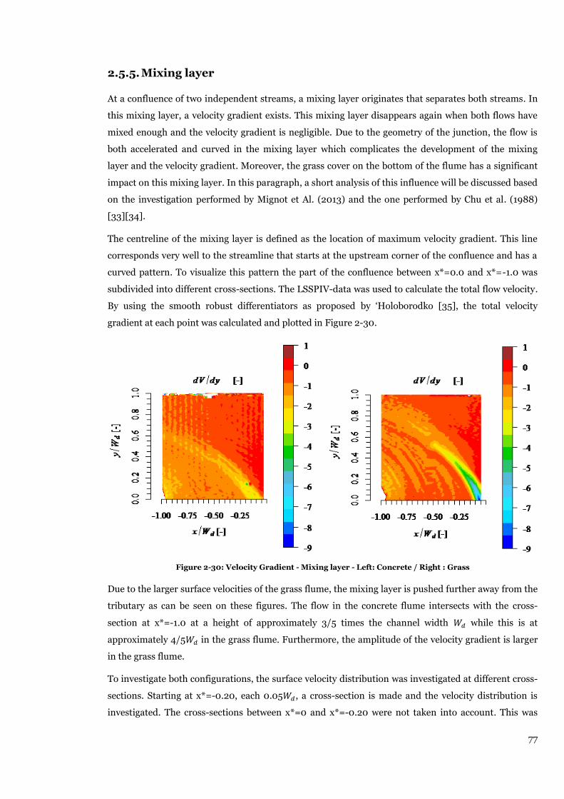
77

Mixing layer 2.5.5.

At a confluence of two independent streams, a mixing layer originates that separates both streams. In

this mixing layer, a velocity gradient exists. This mixing layer disappears again when both flows have

mixed enough and the velocity gradient is negligible. Due to the geometry of the junction, the flow is

both accelerated and curved in the mixing layer which complicates the development of the mixing

layer and the velocity gradient. Moreover, the grass cover on the bottom of the flume has a significant

impact on this mixing layer. In this paragraph, a short analysis of this influence will be discussed based

on the investigation performed by Mignot et Al. (2013) and the one performed by Chu et al. (1988)

[33][34].

The centreline of the mixing layer is defined as the location of maximum velocity gradient. This line

corresponds very well to the streamline that starts at the upstream corner of the confluence and has a

curved pattern. To visualize this pattern the part of the confluence between x*=0.0 and x*=-1.0 was

subdivided into different cross-sections. The LSSPIV-data was used to calculate the total flow velocity.

By using the smooth robust differentiators as proposed by ‘Holoborodko [35], the total velocity

gradient at each point was calculated and plotted in Figure 2-30.

Figure 2-30: Velocity Gradient - Mixing layer - Left: Concrete / Right : Grass

Due to the larger surface velocities of the grass flume, the mixing layer is pushed further away from the

tributary as can be seen on these figures. The flow in the concrete flume intersects with the cross-

section at x*=-1.0 at a height of approximately 3/5 times the channel width while this is at

approximately 4/5 in the grass flume. Furthermore, the amplitude of the velocity gradient is larger

in the grass flume.

To investigate both configurations, the surface velocity distribution was investigated at different cross-

sections. Starting at x*=-0.20, each 0.05 , a cross-section is made and the velocity distribution is

investigated. The cross-sections between x*=0 and x*=-0.20 were not taken into account. This was

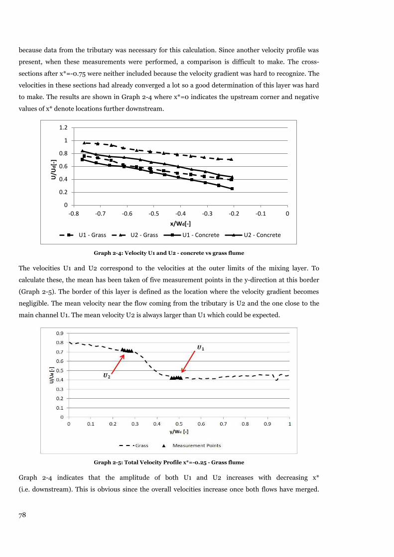
78

because data from the tributary was necessary for this calculation. Since another velocity profile was

present, when these measurements were performed, a comparison is difficult to make. The cross-

sections after x*=-0.75 were neither included because the velocity gradient was hard to recognize. The

velocities in these sections had already converged a lot so a good determination of this layer was hard

to make. The results are shown in Graph 2-4 where x*=0 indicates the upstream corner and negative

values of x* denote locations further downstream.

Graph 2-4: Velocity U1 and U2 - concrete vs grass flume

The velocities U1 and U2 correspond to the velocities at the outer limits of the mixing layer. To

calculate these, the mean has been taken of five measurement points in the y-direction at this border

(Graph 2-5). The border of this layer is defined as the location where the velocity gradient becomes

negligible. The mean velocity near the flow coming from the tributary is U2 and the one close to the

main channel U1. The mean velocity U2 is always larger than U1 which could be expected.

Graph 2-5: Total Velocity Profile x*=-0.25 - Grass flume

Graph 2-4 indicates that the amplitude of both U1 and U2 increases with decreasing x*

(i.e. downstream). This is obvious since the overall velocities increase once both flows have merged.

0

0.2

0.4

0.6

0.8

1

1.2

-0.8 -0.7 -0.6 -0.5 -0.4 -0.3 -0.2 -0.1 0

U/U

d[-

]

x/Wd[-]

U1 - Grass U2 - Grass U1 - Concrete U2 - Concrete

79

However, the velocity difference over the mixing layer is not equal for the concrete configuration and

the grass configuration as shown in Graph 2-6.

Graph 2-6: ΔU - Concrete vs Grass flume

The velocity difference decreases in both configurations with decreasing x*. This is obvious since both

flows have to converge towards a uniform flow. The velocity difference is larger in the grass flume than

in the concrete flume. The difference decreases only a little bit in the concrete flume, while this value

decreases in the grass flume with half of its initial value. This can be explained when looking at the

overall flow pattern of the confluence. In the concrete configuration at the upstream corner, the

velocities remain low in both tributary and main channel. So at the first cross-section that was plotted,

only a small velocity variation can be spotted. Further downstream, the flow velocities increase, but

both flows start to merge so the overall effect will stagnate. At the grass configuration, the velocity

difference at the upstream corner is more pronounced. Because of this, the shearing effect will be

larger and the flow velocities will converge at a faster rate.

When looking at Graph 2-7, the velocity gradient decreases when going downstream. Since both flows

converge, this velocity gradient has to decrease so a single flow remains.

Graph 2-7: Maximum Velocity Gradient - Concrete vs Grass flume

0

0.05

0.1

0.15

0.2

0.25

0.3

0.35

-0.8 -0.7 -0.6 -0.5 -0.4 -0.3 -0.2 -0.1 0

ΔU

/U0[-

]

x/Wd[-]

Grass Concrete

00.5

11.5

22.5

33.5

44.5

-0.8 -0.7 -0.6 -0.5 -0.4 -0.3 -0.2 -0.1 0

max

(dU

/dy)

[-]

x/Wd [-]

Grass Concrete

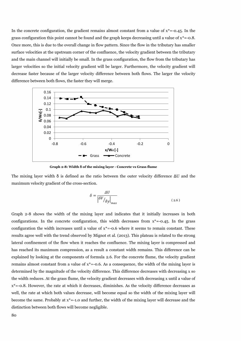
80

In the concrete configuration, the gradient remains almost constant from a value of x*=-0.45. In the

grass configuration this point cannot be found and the graph keeps decreasing until a value of x*=-0.8.

Once more, this is due to the overall change in flow pattern. Since the flow in the tributary has smaller

surface velocities at the upstream corner of the confluence, the velocity gradient between the tributary

and the main channel will initially be small. In the grass configuration, the flow from the tributary has

larger velocities so the initial velocity gradient will be larger. Furthermore, the velocity gradient will

decrease faster because of the larger velocity difference between both flows. The larger the velocity

difference between both flows, the faster they will merge.

Graph 2-8: Width δ of the mixing layer - Concrete vs Grass flume

The mixing layer width δ is defined as the ratio between the outer velocity difference ΔU and the

maximum velocity gradient of the cross-section.

| ⁄ |

( 2.6 )

Graph 2-8 shows the width of the mixing layer and indicates that it initially increases in both

configurations. In the concrete configuration, this width decreases from x*=-0.45. In the grass

configuration the width increases until a value of x*=-0.6 where it seems to remain constant. These

results agree well with the trend observed by Mignot et al. (2013). This plateau is related to the strong

lateral confinement of the flow when it reaches the confluence. The mixing layer is compressed and

has reached its maximum compression, as a result a constant width remains. This difference can be

explained by looking at the components of formula 2.6. For the concrete flume, the velocity gradient

remains almost constant from a value of x*=-0.6. As a consequence, the width of the mixing layer is

determined by the magnitude of the velocity difference. This difference decreases with decreasing x so

the width reduces. At the grass flume, the velocity gradient decreases with decreasing x until a value of

x*=-0.8. However, the rate at which it decreases, diminishes. As the velocity difference decreases as

well, the rate at which both values decrease, will become equal so the width of the mixing layer will

become the same. Probably at x*=-1.0 and further, the width of the mixing layer will decrease and the

distinction between both flows will become negligible.

0

0.02

0.04

0.06

0.08

0.1

0.12

0.14

0.16

-0.8 -0.6 -0.4 -0.2 0

δ/W

d[-

]

x/Wd [-]

Grass Concrete

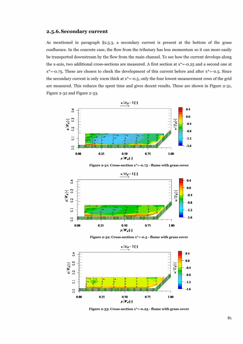
81

Secondary current 2.5.6.

As mentioned in paragraph §2.5.3, a secondary current is present at the bottom of the grass

confluence. In the concrete case, the flow from the tributary has less momentum so it can more easily

be transported downstream by the flow from the main channel. To see how the current develops along

the x-axis, two additional cross-sections are measured. A first section at x*=-0.25 and a second one at

x*=-0.75. These are chosen to check the development of this current before and after x*=-0.5. Since

the secondary current is only 10cm thick at x*=-0.5, only the four lowest measurement rows of the grid

are measured. This reduces the spent time and gives decent results. These are shown in Figure 2-31,

Figure 2-32 and Figure 2-33.

Figure 2-31: Cross-section x*=-0.75 - flume with grass cover



82

These figures show the location of the recirculation cell which has a clockwise rotating motion near the

bottom of the flume. In the upstream section (x*=-0.25), the cell has a significant smaller size

compared to the other ones. The cell size increases when going downstream. This increase can be seen

in both the width and the height of the cell. The width increases from 0.20m to approximately 0.40m

at x*=-0.75 and the height of the cell increases from 0.07 Wd at x*=-0.25 to a height of approximately

0.15Wd at x*=-0.75. Another difference is the larger longitudinal-component of the velocity in the

recirculation area when going further downstream. At x*=-0.25 this component is small and the zone

can hardly be seen. At x*=-0.75, this velocity component has increased towards a value that cannot be

neglected. This shows that an important undercurrent is present at the confluence. The flow that goes

over this recirculation area transforms its lateral component into a longitudinal component and is

transported downstream.

Furthermore, the initiation of this recirculation area starts further into the main channel when moving

downstream. At x*=-0.25, this zone starts at y*=0.05 while at x*=-0.50, the zone starts at y*=0.10 and

at x*=-0.75, this is approximately y*=0.20. A lateral shift has occurred from up to downstream. This

counters the possibility that this recirculation area is initiated by a bed discordance caused by two

grass covers that do not match exactly. Since two grass covers meet at the confluence, a height

difference could be present. When this is the case, the recirculation area should start at y*=0 in every

cross-section and the growth of this cell would not be as large as it is now. This lateral shift is also

present at Figure 2-26 at the bottom. The zone with upstream current at the bottom decreases in size

from the right bank to the left. This represents the lateral shift of this secondary cell.

The location of this recirculation area is approximately equal to the location of the mixing layer. This

mixing layer, as mentioned in §2.5.5 starts at the upstream corner and has a curved pattern towards

the right side of the flume (looking downstream). Table 2-7 shows a comparison of the LSSPIV data

and the ADV data. With the ADV data, the location of the recirculation cell was determined, while the

location of the mixing layer at the water surface was measured with the LSSPIV data. This

measurement is based on the location of the largest velocity gradient in each of these cross-sections.

The location of the recirculation area was guessed from the figures on the previous page.

Table 2-7: Location shear layer vs recirculation area

y* - LSSPIV y* - ADV

x*=-0.25 0.36 0.25

x*=-0.50 0.57 0.50

x*=-0.75 0.71 0.65

A comparison between both data is rather difficult since the LSSPIV-data is monitored at the water

surface and the ADV data at the bottom of the flume. Due to the skewed shape of the shear plane, these

locations can differ. However, the location of the recirculation area is always close to the location of the

mixing layer. The recirculation area is located closer to the left than the maximum velocity gradient.

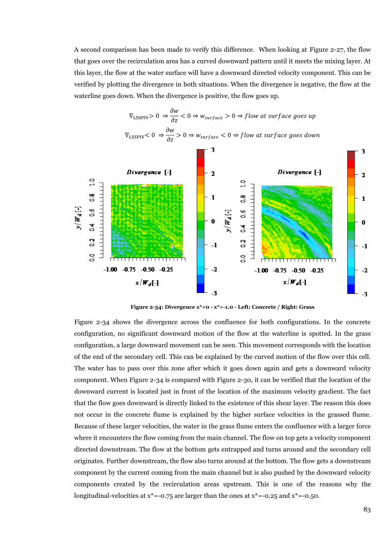
83

A second comparison has been made to verify this difference. When looking at Figure 2-27, the flow

that goes over the recirculation area has a curved downward pattern until it meets the mixing layer. At

this layer, the flow at the water surface will have a downward directed velocity component. This can be

verified by plotting the divergence in both situations. When the divergence is negative, the flow at the

waterline goes down. When the divergence is positive, the flow goes up.

Figure 2-34: Divergence x*=0 - x*=-1.0 - Left: Concrete / Right: Grass

Figure 2-34 shows the divergence across the confluence for both configurations. In the concrete

configuration, no significant downward motion of the flow at the waterline is spotted. In the grass

configuration, a large downward movement can be seen. This movement corresponds with the location

of the end of the secondary cell. This can be explained by the curved motion of the flow over this cell.

The water has to pass over this zone after which it goes down again and gets a downward velocity

component. When Figure 2-34 is compared with Figure 2-30, it can be verified that the location of the

downward current is located just in front of the location of the maximum velocity gradient. The fact

that the flow goes downward is directly linked to the existence of this shear layer. The reason this does

not occur in the concrete flume is explained by the higher surface velocities in the grassed flume.

Because of these larger velocities, the water in the grass flume enters the confluence with a larger force

where it encounters the flow coming from the main channel. The flow on top gets a velocity component

directed downstream. The flow at the bottom gets entrapped and turns around and the secondary cell

originates. Further downstream, the flow also turns around at the bottom. The flow gets a downstream

component by the current coming from the main channel but is also pushed by the downward velocity

components created by the recirculation areas upstream. This is one of the reasons why the

longitudinal-velocities at x*=-0.75 are larger than the ones at x*=-0.25 and x*=-0.50.

84

Divergence plots of the separation zone are shown in Figure 2-35. One clearly distinguishes a relative

big upward motion (positive values) for the grass configuration while this upward motion is almost

absent at the concrete flume. At the grass flume, the water moves upward near the left bank and goes

down again close the shear layer. Between both actions, the water moves lateral towards the right

bank. These observations were also seen in the LSSPIV-vector plots (Figure 2-21 and Figure 2-22) and

the velocity contour plots in the y-direction (Figure 2-24). These plots indicate a lateral motion away

from the left bank towards the shear layer. This current is absent at the concrete configuration where

the fluid only has an upstream velocity component. These findings were confirmed with visual

observations of the tracer particles. In the grass flume they move under an oblique angle with an

upstream component and a lateral component towards the right bank. The particles of the concrete

case only have an upstream velocity component.

Figure 2-35: Divergence at separation zone – left: Concrete / right: Grass

85

Shear planes and vorticity 2.5.7.

The available data from the LSSPIV can be used to get more information about the instability of the

shear planes. First, the instability of the shear planes will be analysed in an optical way. Two different

shear planes are present, one originating at the upstream corner and ending at the reattachment point

and a second one going from the downstream corner until the end of the separation zone. These shear

planes are visualised in Figure 2-36 and in the real situation (Figure 2-37).

Figure 2-36: Indication of shear planes

Figure 2-37: Frame of the existing confluence where the shear planes are visualized with tracers

LSSPIV-frames from the grass configuration are shown in Figure 2-38 (x*=0 to x*=0.66), Figure 2-39

(x*=-1.02 to x*=-1.69) and Figure 2-40 (x*=-1.50 to x*=-2.16). These frames only give an

instantaneous impression of the situation, but are chosen attentively so they give a good

representation of the global flow pattern. Figure 2-38 shows that the tracers follow a curved track and

do not rotate around their axis. The red line on the figure represents the mixing layer. Because most

tracers do not rotate, no vortices are created along the shear plane.

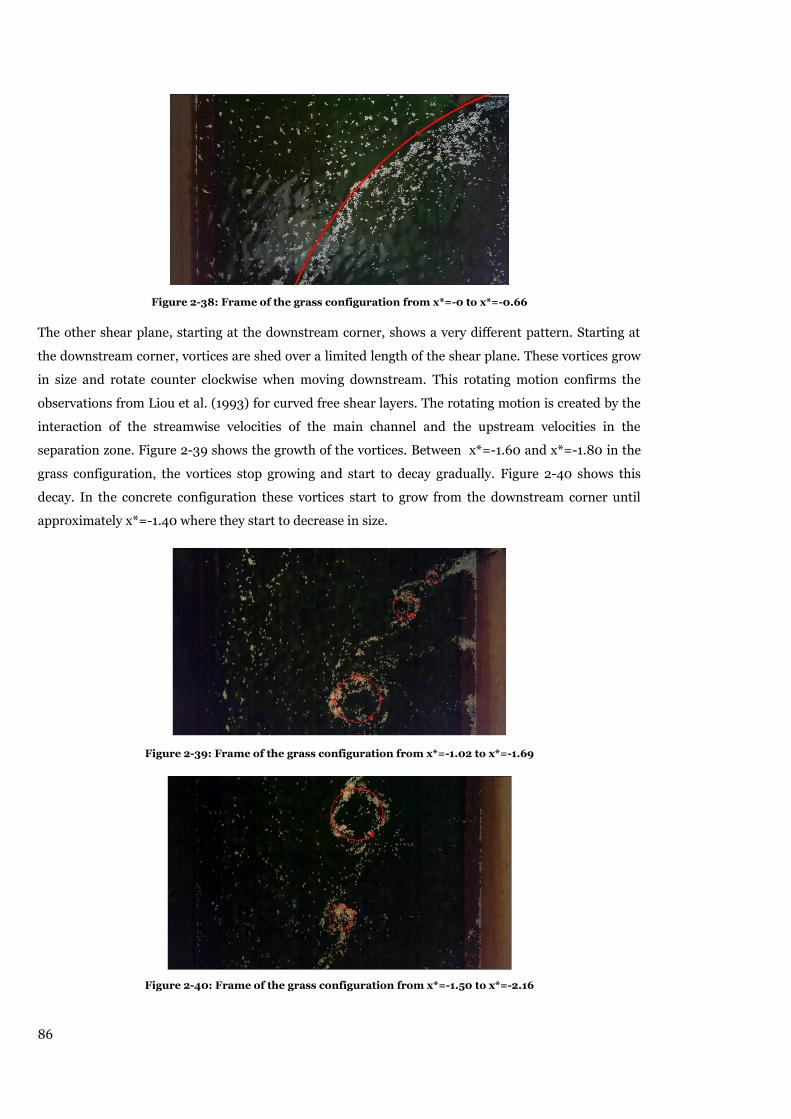
86

Figure 2-38: Frame of the grass configuration from x*=-0 to x*=-0.66

The other shear plane, starting at the downstream corner, shows a very different pattern. Starting at

the downstream corner, vortices are shed over a limited length of the shear plane. These vortices grow

in size and rotate counter clockwise when moving downstream. This rotating motion confirms the

observations from Liou et al. (1993) for curved free shear layers. The rotating motion is created by the

interaction of the streamwise velocities of the main channel and the upstream velocities in the

separation zone. Figure 2-39 shows the growth of the vortices. Between x*=-1.60 and x*=-1.80 in the

grass configuration, the vortices stop growing and start to decay gradually. Figure 2-40 shows this

decay. In the concrete configuration these vortices start to grow from the downstream corner until

approximately x*=-1.40 where they start to decrease in size.

Figure 2-39: Frame of the grass configuration from x*=-1.02 to x*=-1.69

Figure 2-40: Frame of the grass configuration from x*=-1.50 to x*=-2.16

87

In both configurations, the size and quantity of these vortices was monitored. In the grass

configuration, fewer vortices were present compared to the concrete one but their average size was

larger. In the concrete flume, their dimensions varied more from very small to very large so no clear

trend could be drawn. As mentioned before, they start to decay faster so this layer becomes stable at an

earlier section.

Figure 2-41 shows the vorticity distribution at the mixing layer of the confluence. This shear layer

starts at the upstream corner and proceeds downstream. Calculation of these values was performed

using the velocities calculated with the robust smooth differentiator. The vorticity was then calculated

with the following formula:

( 2.7 )

Figure 2-41: Vorticity - mixing layer – left: concrete / right: grass

Both figures indicate the vorticity at the mixing layer which remains low. The blue regions on top of

both figures do not indicate vortices, but just mark the presence of the border. Because of this border,

the velocity gradient is large at this location which results in large amplitudes of the vorticity.

In both situations, vortices are present but are small and decrease rapidly in size. To check if

instability at the mixing layer can be predicted, the Fjörtoft criterion will be used. To trigger instability,

a vorticity extremum and an inflection point in the velocity profile have to be present at the same

location. The velocity profiles at the mixing layer were already studied in §2.5.5. In this paragraph,

only the sections between x*=-0.20 and x*=-0.75 were examined. Since the inflection point at

locations further downstream was difficult to find, instability will not occur at these locations. An

inflection point at the cross-section between x*=0 and x*=-0.20 is assumed to be present, so these will

also be considered to check instability. One condition to have instability according to Fjörtoft, is that

the vorticity has to reach a maximum or minimum.

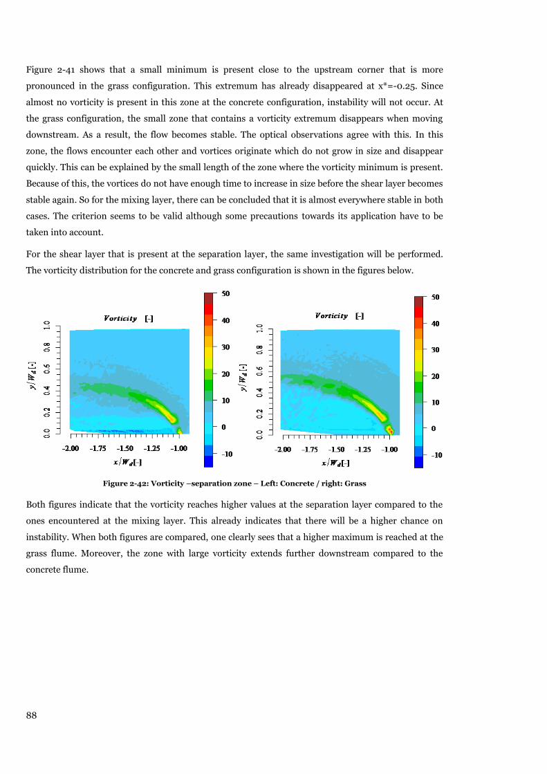
88

Figure 2-41 shows that a small minimum is present close to the upstream corner that is more

pronounced in the grass configuration. This extremum has already disappeared at x*=-0.25. Since

almost no vorticity is present in this zone at the concrete configuration, instability will not occur. At

the grass configuration, the small zone that contains a vorticity extremum disappears when moving

downstream. As a result, the flow becomes stable. The optical observations agree with this. In this

zone, the flows encounter each other and vortices originate which do not grow in size and disappear

quickly. This can be explained by the small length of the zone where the vorticity minimum is present.

Because of this, the vortices do not have enough time to increase in size before the shear layer becomes

stable again. So for the mixing layer, there can be concluded that it is almost everywhere stable in both

cases. The criterion seems to be valid although some precautions towards its application have to be

taken into account.

For the shear layer that is present at the separation layer, the same investigation will be performed.

The vorticity distribution for the concrete and grass configuration is shown in the figures below.

Figure 2-42: Vorticity –separation zone – Left: Concrete / right: Grass

Both figures indicate that the vorticity reaches higher values at the separation layer compared to the

ones encountered at the mixing layer. This already indicates that there will be a higher chance on

instability. When both figures are compared, one clearly sees that a higher maximum is reached at the

grass flume. Moreover, the zone with large vorticity extends further downstream compared to the

concrete flume.

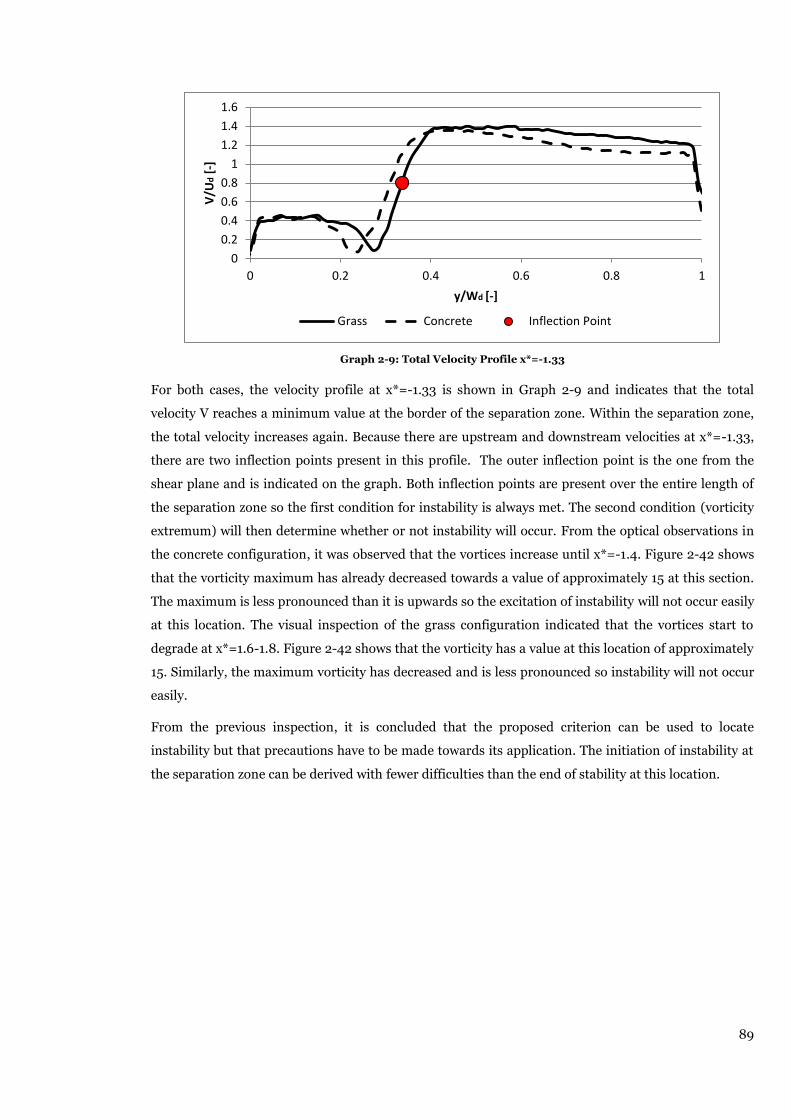
89

Graph 2-9: Total Velocity Profile x*=-1.33

For both cases, the velocity profile at x*=-1.33 is shown in Graph 2-9 and indicates that the total

velocity V reaches a minimum value at the border of the separation zone. Within the separation zone,

the total velocity increases again. Because there are upstream and downstream velocities at x*=-1.33,

there are two inflection points present in this profile. The outer inflection point is the one from the

shear plane and is indicated on the graph. Both inflection points are present over the entire length of

the separation zone so the first condition for instability is always met. The second condition (vorticity

extremum) will then determine whether or not instability will occur. From the optical observations in

the concrete configuration, it was observed that the vortices increase until x*=-1.4. Figure 2-42 shows

that the vorticity maximum has already decreased towards a value of approximately 15 at this section.

The maximum is less pronounced than it is upwards so the excitation of instability will not occur easily

at this location. The visual inspection of the grass configuration indicated that the vortices start to

degrade at x*=1.6-1.8. Figure 2-42 shows that the vorticity has a value at this location of approximately

15. Similarly, the maximum vorticity has decreased and is less pronounced so instability will not occur

easily.

From the previous inspection, it is concluded that the proposed criterion can be used to locate

instability but that precautions have to be made towards its application. The initiation of instability at

the separation zone can be derived with fewer difficulties than the end of stability at this location.

0

0.2

0.4

0.6

0.8

1

1.2

1.4

1.6

0 0.2 0.4 0.6 0.8 1

V/U

d [

-]

y/Wd [-]

Grass Concrete Inflection Point

91

2.6. Conclusion

Experiments were done to investigate the influence of a grass cover on the flow characteristics at a

confluence. LSSPIV was used to measure velocity patterns at the water surface, while the ADV was

used to measure the flow features at different cross-sections. In this way, the complex flow pattern at a

confluence was investigated in three dimensions.

The ADV-reference measurements indicated that the possible error by choosing a time frame of 2min

(instead of 10min) is negligible in the x and y-direction. This error is slightly bigger in z-direction

because here, the velocities are much smaller compared to the x and y-direction which results in more

sensitivity to deviations. To conclude, the choice of a time frame of 2min was justified. The

reproducibility of the ADV data was checked by means of confidence intervals. This interval is small

for velocities in the x and y-direction but is large in z-direction. For the concrete flume, the standard

deviation reaches a value that is two times larger than the mean value. As a result, the velocities in

z-direction should be interpreted with care.

Because of the limited length of the tributary, the flow is not fully developed when it reaches the

confluence. Different measurements upstream in the tributary, show altered velocity profiles. This is

probably caused by a shift of the filter at the tributary. As a consequence, attention has to be paid when

comparing ADV-data at y*=0 and x*=-0.5. The surface velocities of the LSSPIV were compared with

the ADV-data just below the water surface in order to check their compatibility. This was done for

every cross-section and gave decent results. Both the shape and the magnitude of the velocity profile

were comparable.

By equipping the flume with the grass cover, a different velocity profile was obtained with lower

velocities close to the bottom. Since the water level differences between the concrete and the grass

flume are almost negligible, the water has to pass a smaller area with an equal flow rate. This causes

larger velocities in the upper part of the cross-section while the flow at the bottom is retarded due to

the additional roughness. Since the discharge of the tributary is three times larger than the one of the

main channel, this change in velocity profile is more pronounced in the tributary. As a result,

momentum from the tributary pushes the shear layer further away from the side channel. The flow

coming from the main channel is more compressed so the separation zone can expand more in width,

whereas it decreases in length. Furthermore, the ratio of the width to length of the separation zone

increases. which agrees with the numerical simulations of Creëlle et al. (2014).

The depth of the recirculation zone is limited by the effect of the chamfer and the return flow to the left

bank located just above the channel bottom. This return flow will bend upwards in the separation zone

resulting in a lateral velocity component towards the right bank. This phenomenon does not appear for

the concrete case because here, the inflow velocities are smaller and do not have the power to reach the

left bank after the collision with the stream of the main channel. As a consequence, the flow in the

separation zone has only an upstream velocity component. These observations were confirmed in

divergence plots of the flow. Another difference is the existence of a secondary current in the flume

92

with the grass cover. This current rotates clockwise just above the channel bed and increases in size

when moving downstream. At x*=-0.25, it is hardly present while it is not negligible for x*=-0.50 and

x*=-0.75. Furthermore the initiation of this recirculation area starts further into the main channel

when moving downstream. . In the concrete case, this cell is absent because the flow from the tributary

has less momentum so it can more easily be transported downstream by the flow from the main

channel.

Visual observations showed that only vortices originate at the shear layer of the separation zone. The

Fjörtoft criterion was used to check the instability of the shear layers and to confirm the visual

observations. For both shear layers, the inflection point is present in the velocity profile but only the

shear layer originating at the downstream corner shows a clear vorticity extremum at the same

location of the inflection point. As a result, only this shear will be unstable and only here vortices will

be shed.

93

Bibliography

[1] L. Leopold, M. Wolman and J. Miller, Fluvial processes in geomorphology, Freeman: San Francisco,

1964.

[2] M. Yalin, Mechanics of sediment transport, Oxford, UK.: Pergamon, 1977.

[3] H. Rouse, “Critical analysis of open-channel resistance,” Journal of the Hydraulics Division, vol. 91, no.

4, pp. 1-15, 1965.

[4] A. Kolmogorov, “Dissipation of energy in the locally isotropic turbulence,” Proceedings of the USSR

Academy of Sciences, vol. 32, pp. 16-18, 1941.

[5] V. Chow, “Chapter 8,” in Theoretical concepts of boundary layer, surface roughness,velocity

distribution and instability of uniform flow, 1959, pp. 192-199.

[6] M. Kleinhans, “Hydraulic roughness,” Utrecht University, [Online]. Available:

www.geog.uu.nl/fg/mkleinhans/teaching/rivmorrough.pdf. [Accessed 27 May 2014].

[7] I. Nezu and M. Sanjou, “Turbulence structure and coherent motion in vegetated canopy open-channel

flows,” Journal of Hydro-environment research 2, 2008.

[8] H. Nepf and E. Vivoni, “Flow structure in depth-limited, vegetated flow,” Journal of geophysical

research vol.105, 2000.

[9] M. Ghisalberti and H. Nepf, “The structure of the shear layer over rigid and flexible canopies,”

Environmental Fluid Mechanics, vol. 6, pp. 277-301, 2006.

[10] M. Raupach, J. Finnigan and Y. Brunet, “Coherent eddies and turbulece in vegetation canopies: the

mixing-layer analogy,” Centre for Environmental Mechanics, 1996.

[11] H. Nakagawa and I. Nezu, “Prediction of the contributions to the Reynolds stress from bursting events

in open-channel flows,” Journal of Fluid Mechanics, vol. 80, pp. 99-128, 1977.

[12] N. Kauwen and T. Unny, “Flexible roughness in open channel,” Journal of the Hydraulics Division, vol.

99, no. 5, pp. 713-728, 1973.

[13] C. Wilson, A. Batemann-Pinzen, P. Bates and T. Stoesser, “Open channel flow through different forms

of submerged flexible vegetation,” Journal of Hydraulic Engineering, vol. 129, no. 11, pp. 847-853,

2003.

[14] F. Wu, H. Sheh and Y. Chou, “Variation of roughness coefficients for unsubmerged and submerged

vegetation,” Journal of hydraulic Engineering, pp. 934-942, 1999.

[15] I. Nezu, H. Nakagawa and W. Rodi, “Significant difference between secondary currents in closed

channels and narrow open channels,” pp. A125-A132, 1989.

94

[16] E. Shumate, Experimental description of flow at an open-channel junction, Unpublished master thesis,

University of Iowa, Iowa, 1998.

[17] J. Best and I. Reid, “Separation zone at open channel junctions,” Journal of Hydraulic Engineering,

vol. 110, no. 11, pp. 1588-1594, 1984.

[18] L. Crombé, “Numerieke modellering van een riviersamenvloeiing: Onderzoek naar de invloed van

vegetatie op de stromingspatronen (Unpublished master thesis),” no. University of Ghent, 2012.

[19] S. Creëlle, T. De Mulder, L. Schindfessel and T. Van Oyen, “Influence of hydraulic resistance on flow

features in an open channel confluence: Accepted in de Almeide(ed.),” in Proc. 3rd IAHR Europe

Congress, Porto, 13-17 April 2014.

[20] J. Huang, L. Weber and Y. Lai, “Three dimensional numerical study of flows in open-channel

junctions,” Journal of hydraulic engineering, pp. 268-280, 2002.

[21] C. Hsu, F. Wu and W. Lee, “Flow at a 90° equal-width open-channel junction,” Journal of Hydraulic

Engineering, vol. 124, no. 2, pp. 186-191, 1998.

[22] P. Biron, J. Best and A. Roy, “Effects of bed discordance on flow dynamics at open channel

confluences,” Journal of Hydralic Engineering vol. 122, pp. 676-682, 1996.

[23] P. Drazin and W. Reid, “Introduction to hydrodynamic stability,” pp. 138-180.

[24] J. Bell and R. Metha, “Development of a two-stream mixing layerfrom tripped and untripped boundary

layers,” AIAA journal, vol. 28, no. 12, pp. 2034-2042, 1990.

[25] W. Liou, “Linear instability of curved free shear layers,” Phys. Fluids 6, pp. 541-548, 1993.

[26] H. Fiedler, J.-H. Kim and N. Köpp, “The spatially accelerated mixing layer in a tailored pressure

gradient,” European Journal of Mechanics, vol. 10, no. 4, pp. 349-376, 1991.

[27] V. Chu, J. Wu and R. Khayat, “Stability of transverse shear flows in shallow open channels,” Journal of

Hydraulic Engineering, vol. 127, pp. 351-368, 1991.

[28] R. Fjortoft, “Application of integral theorems in deriving criteria of stability for laminar flows and for

the baroclinic circular vortex,” Geophys. Publ., vol. 17, pp. 1-52, 1950.

[29] M. Khublaryan, “Surface Waters: Rivers, Streams, Lakes and Wetlands.,” in Types and Properties of

Water, Oxford: EOLSS Publischers Co. Ltd, 2009.

[30] R. Keane and R. Adrian, “Theory of cross-correlation analysis of PIV images,” Applied Scientific

Research, pp. 191-215, 1992.

[31] D. G. Goring and V. I. Nikora, “Discussion of "Despiking Acoustic Doppler Velocimeter Data" by Derek

G. Goring and Vladimir I. Nikora,” Journal of Hydraulic Engineering vol. 129, pp. 484-487, 2003.

95

[32]

T. Wahl, “Despiking acoustic Doppler velocimeter Data. discussion,” Journal of Hydraulic Engineering,

vol. 129, no. 6, pp. 484-487, 2003.

[33] E. Mignot, I. Vinkovic, D. Doppler and N. Riviere, “Mixing layer in open-channel junction flows,”

Environmental Fluid Mechanics, 2013.

[34] V. Chu and S. Babarutsi, “Confinement and bed-friction effects in shallow turbulent mixing layers,”

Journal of hydraulic engineering vol.114, pp. 1257-1273, 1988.

[35] Holoborodko, “www.holoborodko.com,” [Online]. Available:

http://www.holoborodko.com/pavel/numerical-methods/numerical-derivative/smooth-low-noise-

differentiators/. [Accessed 3 Mai 2014].

[36] H. Fernando, “Handbook of environmental fluid dynamics, volume one: overview and fundamentals,”

2013, pp. 289-291.

[37] L. Weber, Schumate, E. Shumate and N. Mawer, “Experiments on flow at 90° open-channel junction,”

Journal of Hydraulic Engineering vol.127, pp. 340-350, 2001.

[38] B. Barkdoll, “Discussion of "experiments on flow at an 90° open channel junction" by Larry J. Weber,

Eric D. Shumate, and Nicola Mawer,” Hydraulic Engineering vol. 127, pp. 340-350, 2001.

[39] B. White and H. Nepf, “A vortex based model of velocity and shear stress in a partially vegetated

shallow channel,” Water resources research vol.44, 2008.

[40] B. Stone and H. Shen, “Hydraulic resistance of flow in channels with cylindrical roughness,” Journal of

Hydraulic Engineering vol. 128, pp. 500-506, 2002.

[41] D. Vermaas, W. Uijttewaal and A. Hoitink, “Lateral transfer of streamwise momentum caused by

roughness transition across a shallow channel,” Water resources research vol. 47, 2011.

[42] L. Schindfessel, S. Creëlle, T. Boelens and T. De Mulder, “Flow patterns in an open channel confluence

with a small ratio of main chanel to tributary discharge,” Ghent University, 2014.

[43] H. Fisher and T. Hanamura, “The effect of roughness strips on transverse mixing in hydraulic models,”

Water resources research vol.11 No 1, pp. 362-364, 1975.

[44] D. Goring and V. Nikora, “Despiking Acoustic Doppler Velocimeter Data,” Journal of Hydraulic

Engineering vol.128, pp. 117-126, 2002.

[45] G. Katul, G. Kuhn, J. Schieldge and C. Hsieh, “The ejection-sweep character of scalar fluxes in the

unstable surface layer,” 1996.

[46] M. Muste, I. Fujita and A. Hauet, “Large-scale particle image velocimetry for measurements in riverine

environments,” Water resources research vol. 44, 2008.

[47] K. Bradbrook, S. Lane, K. Richards, P. Brion and A. Roy, “Role of bed discordance at asymmetrical

river confluences,” Journal of Hydraulic Engineering vol. 127, pp. 351-368, 2001.

96

[48] H. Schlichting and K. Gersten, Boundary layer theory.

[49] S. Leonardi, P. Oriandi and R. Antonia, “Properties of d-type and k-type roughness in turbulent

channel flows,” Physics of fluids, 2007.

[50] T. Saad, “Turbulence modelling for beginners,” University of Tenessee Space institute.

[51] S. Otto, T. Jackson and F. Hu, “On the spatial evolution of centrifugal instabilities with curved

incompressible mixing lyaer,” Journal of Fluid mechanics vol. 315, pp. 85-103, 1996.

[52] J. Jarvela, “Flow resistance of flexible and stiff vegetation: af flume study with natural plants,” Journal

of Hydrology vol.269, pp. 44-54, 2002.

[53] B. Yen, “Open channel flow resistance,” Journal of hydraulic engineering, vol. 128, pp. 20-39, 2002.

[54] H. Nepf, “drag, turbulence and diffusion in flow through emergent vegetatoin,” Water resources

research vol.35, 1999.

[55] J. Green, “Modelling flow resistance in vegetated streams: review and development of new theory,”

Hydrological Processes 19, pp. 1245-1259, 2005.

[56] Environmental fluid mechanics chapter 5: Instabilities, Darthmounth college: Thayer school of

engineering, pp. 103-125.

[57] “National committee for fluid mechanics films,” [Online]. Available:

http://web.mit.edu/hml/ncfmf.html. [Accessed 17 March 2014].

[58] A. Galema, “Vegetation resistance evaluation of vegetation resistance descriptors for flood

management (Unpublished master thesis),” 2009.

[59] G. Arcement and V. Schneider, “Guide for selecting Mannings's roughness coefficients for Natural

channels and flood plaines,” United States Geological Survey Water-Supply, 1989.

[60] F. Carollo, V. Ferro and D. Termini, “ Flow resistance law in channels with flexible submerged

vegetation,” Journal of Hydraulic research, vol. 131, pp. 554-564, 2005.

[61] M. A. I. Nezu, “Open-channel Flow Turbulence and its research prospect in the 21st century,” Journal

of Hydraulic Engineering, pp. 229-246, 2005.

[62] P. Davidson, “Turbulence: An introduction for scientists and engineers,” Oxford University Press,

2004, p. 19.

[63] C. Polatel, “Large-Scale roughness effect on free-surface and bulk flo9w characteristics in open-channel

flows,” Iowa, 2006.

Study of the influence of bed roughness on the flow ...

Documents

Transcript of Study of the influence of bed roughness on the flow ...