ABB Contactors - 4 Pole Contactors ABB AF09 AF09Z (AC DC) Contactors
Study of gas-liquid flow contactors using
low-intrusive measuring technology
Dissertation
zur
Erlangung des akademischen Grades eines
Dr.-Ing.
der
Fakultät Maschinenbau
der Ruhr-Universität Bochum
von
Dipl. -Ing. Guanghua Zheng
aus
Jilin, China
Bochum 2017

Dissertation eingereicht am: 06. Dezember 2017
Tag der mündlichen Prüfung: 04. Mai 2018
Erster Referent: Prof. Dr.-Ing. Marcus Grünewald
Zweiter Referent: Prof. Dr.-Ing. Uwe Hampel
Danksagung
Die vorliegende Arbeit entstand während meiner Tätigkeit als wissenschaftlicher
Mitarbeiter am Lehrstuhl für Fluidverfahrenstechnik der Fakultät Maschinenbau
der Ruhr-Universität Bochum.
Mein besonderer Dank gilt dem Inhaber des Lehrstuhls für Fluidverfahrens-
technik, Herrn Prof. Dr.-Ing. Marcus Grünewald, für die Überlassung des
Promotionsthemas, das Vertrauen in die Wichtigkeit messtechnischer
Fragestellungen bei der Untersuchung von Mehrphasenapparaten und vor allem
für die vielfältige Unterstützung.
Herrn Prof. Dr.-Ing. Uwe Hampel danke ich für die Erstellung des Zweitgutachtens.
Darüber hinaus bedanke ich mich bei den Kollegen am Lehrstuhl für
Fluidverfahrenstechnik für die gute Arbeitsatmosphäre und den fachlichen
Austausch. Insbesondere danke ich Melanie Bothe, Manuela Kopatschek und
Corinna Hecht für die gegenseitige Unterstützung und die angenehme gemeinsame
Zeit.
Viele wertvolle Anregungen und Diskussionen habe ich darüber hinaus aus den im
Rahmen der Forschungsarbeiten durchgeführten Studien-, Projekt- und Diplom-
arbeiten von J. Yan, S. Wu, P. Biessey, N. Abel, M. Dippel, T. Sonau, P. Zheng, C. Zhao,
K. Keshk, I. Moltup, J. Huang, J. Xin, Z. Li und W. Li erhalten.
Nicht zuletzt gilt mein Dank auch meinen lieben Eltern, meiner Frau und meiner
Tochter, die mit ihrer andauernden Geduld, ihrem Verständnis und ihrer
Unterstützung viel zum Gelingen der vorliegenden Dissertation beigetragen haben.

Content
1 Introduction ............................................................................................................................... 1
2 Measuring methods for measurements of gas-liquid flow pattern ......................................... 3
2.1 Measurements of gas-liquid flow pattern using electrical tomography ................................. 4
2.1.1 Construction and working principle of the WMS ................................................................. 8
2.2 Measurement of gas-liquid flow using the WMS ..................................................................... 8
2.2.1.1 Conductive Wire Mesh Sensor ....................................................................................... 9
2.2.1.2 Capacitive Wire Mesh Sensor ....................................................................................... 11
2.2.2 Electric field simulation of capacitive WMS (own studies) ................................................ 14
2.2.2.1 Permittivity model of the capacitive WMS .................................................................. 14
2.2.2.2 Parameters of the capacitive WMS .............................................................................. 16
2.2.2.3 Finite element method ................................................................................................. 17
2.2.2.4 Two-dimensional electric field simulation .................................................................. 18
2.2.2.4.1 Influence of bubble shape on capacitance ........................................................... 20
2.2.2.4.2 Influence of bubble position on capacitance ....................................................... 20
2.2.2.4.3 Influence of bubble fraction on capacitance ....................................................... 21
2.2.2.4.4 Study of influence of medium permittivity on capacitance ................................ 24
2.2.2.5 Three-dimensional electric field simulation ................................................................ 25
2.2.2.5.1 Influence of bubble size on capacitance .............................................................. 25
2.2.2.5.2 Influence of bubble position (in contact to wires) on capacitance ..................... 26
2.2.2.5.3 Influence of bubble position (without contact to wires) on capacitance ............ 27
2.2.3 Discussion ............................................................................................................................. 28
2.3 Measurements of bubble rise velocity and bubble size using optical fiber method ............ 29
2.3.1 Single optical fiber method .................................................................................................. 29
2.3.2 Four optical fiber method .................................................................................................... 30
2.3.3 Double optical fiber method ................................................................................................ 30
2.3.4 Laser doppler anemometer ................................................................................................. 31
2.3.5 Particle image velocimetry .................................................................................................. 31

2.3.6 Optical fiber method ............................................................................................................ 32
3 Study of phase distribution in bubble columns ..................................................................... 34
3.1 Flow regime in bubble columns ............................................................................................. 34
3.2 Experimental measurements of bubble column .................................................................... 36
3.2.1 Measurements of bubble distribution using WMS ............................................................. 36
3.2.1.1 Experimental results of the capacitive WMS ............................................................... 37
3.2.1.2 Conclusion ..................................................................................................................... 44
3.2.2 Measurements of bubble rise velocity and bubble size using an optical fiber method .... 45
3.2.2.1 Experimental setup ....................................................................................................... 45
3.2.2.2 Data processing of measurements using the optical fiber method ............................ 46
3.2.2.3 Experimental measurements of bubble rise velocity using the optical fiber method 49
3.3 Conclusion ............................................................................................................................... 54
4 Study of phase distribution in packed columns ..................................................................... 56
4.1 Theoretical background of packed columns .......................................................................... 56
4.1.1 Pressure drop ....................................................................................................................... 59
4.1.2 Liquid holdup ....................................................................................................................... 61
4.1.3 Loading and flooding points ................................................................................................ 65
4.1.4 Mass transfer process ........................................................................................................... 67
4.1.4.1 Equilibrium model ........................................................................................................ 67
4.1.4.2 Rate-based model .......................................................................................................... 69
4.1.5 Study of phase distribution .................................................................................................. 73
4.2 Experimental study of packed column ................................................................................... 83
4.2.1.1 Study of hydrodynamics in structured packing .......................................................... 85
4.2.1.2 Study of hydrodynamics in random packing .............................................................. 87
4.2.1.3 Mass transfer of structured and random packing ....................................................... 90
4.2.2 Experimental investigation of phase distribution using a liquid collector ........................ 94
4.2.3 Experimental measurements using WMS ........................................................................... 98
4.2.3.1 Experimental measurements of phase distribution in random packed column ....... 98
4.2.3.2 Experimental measurements of phase distribution in structured packed column . 106

4.3 Simulation and Modeling of phase distribution .................................................................. 107
4.3.1 Cell model ........................................................................................................................... 109
4.3.2 Simulation of phase distribution using cell model ........................................................... 116
4.4 Discussion .............................................................................................................................. 119
5 Nomenclature ........................................................................................................................ 121
6 References ............................................................................................................................. 123
Introduction
1
1 Introduction
Packed columns and bubble columns are important apparatuses for gas-liquid
contacting processes.
Packed columns are widely used for gas-liquid or liquid-liquid separation
processes, e.g. absorption, desorption and rectification. In packed columns, the
liquid phase is often assumed to be homogeneously distributed over the column
cross section. So far, large scale maldistribution is not considered in many existing
theoretical models, namely volume-averaged models. The widely used models of
Mersmann [Mersmann and Deixler (1986)], Billet [Billet (1995)], Mackowiak
[Mackowiak (2010)] and Stichlmair [Stichlmair et al. (1989)]) generally constitute
simplified physical models and the parameters of the derived correlations can be
fitted with experimental results. The liquid collecting method, which is used for
measurements of liquid holdups in packed columns, strongly affects the phase
distribution, resulting in less reliable experimental measurements.
Bubble columns are commonly used for gas-liquid reactions in continuous or semi-
batch processes, due to their good heat transfer characteristics and their relatively
simple construction and operation. Since bubble columns are very successfully
applied in the chemical industry, they represent an important type of gas-liquid
contactors. Backmixing of the liquid phase through the gas phase in bubble
columns greatly influences reaction conversion rate and selectivity. Although the
design of bubble columns is simple, the determination of gas and liquid phase
interfacial area is difficult. Dispersion models studied by Deckwer [Deckwer and
Field (1992)] and Becker [Becker et al. (1994)] assumed ideal mixing in the radial
direction. The mixing of the liquid phase through the moving gas phase is also
influenced by the column wall. It is possible to calculate the rise velocity of a single
bubble. However, it is difficult to predict the rise velocity of bubble clusters.
The phase distribution in such gas-liquid contacting devices is often assumed to be
homogeneous. The phase distribution in multiphase flow can significantly
influence the performance and efficiency of mass transfer. Thus, it is essential to
study the phase distribution inside gas-liquid contacting apparatuses. In many
cases, validation of theoretical models with experimental results is still

Introduction
2
unsatisfactory, as the local flow structure and the flow regime are often not
sufficiently described by simplified models.
Many measurement techniques have already been used to measure the phase
distribution in gas-liquid contactors. Recently, new measurement methods, e.g.
electrical resistance/capacitance tomography, reviewed by Chaumat [Chaumat
et al. (2005)], allow measurements of the phase distribution inside gas-liquid
contactors with strongly reduced intrusiveness. The spatial resolution is not
satisfied.
The capacitive wire mesh sensor (WMS) developed by Da Silva [Da Silva et al.
(2007)] [Da Silva and Hampel (2010)] was used for measurements of phase
distributions in this work. The capacitive WMS is in direct contact with both, the
gas and the liquid phase. The phase distribution across the column cross-section
can be measured with high temporal resolution. The spatial resolution of the WMS
depends on the distance between neighbored wires of the WMS.
The capacitive WMS was applied for measurements of the phase distribution in
packed and bubble columns. Additionally, an optical fiber method was applied to
measure bubble size distributions and bubble rise velocity in bubble columns. The
target of this thesis is to study the influences of phase distribution on the process
parameters in packed and bubble columns based on reliable experimental
measurements.
This work attributes to experimental studies of phase distribution in gas-liquid
contactors, that are packed and bubble columns, using conventional and modern
measurement methods. The fraction of the liquid phase close to the wall of packed
columns was measured using an on-wall liquid collector. Large scale
maldistribution was observed. Depending on the packing types and operational
conditions, the phase distribution is discussed individually. The working principle,
advantages and disadvantages of the capacitive WMS are analyzed and discussed.
The capacitive WMS is applied for the measurement of the phase distribution
across the cross section of packed columns, which is the cross-sectional averaged
measuring method. The experimental results in bubble columns using the WMS
and the optical fiber method are discussed. Both methods can be classified as low-

Measuring methods for measurements of gas-liquid flow pattern
3
intrusive methods for gas-liquid contactors. The spatial and temporal resolutions
are proven to be reliable for the study of phase distribution in packed and bubble
columns. Concerning the experimental results with the WMS, a phase distribution
model for packed columns (cell model) is developed. The influence of process
parameters on the phase distribution is discussed on the basis on the cell model
simulation results.
2 Measuring methods for measurements of gas-liquid flow
pattern
Although packed columns and bubble columns are widely used in chemical
industry and separation technology, their local phase distribution is not yet well
known, limited by the measurement methods. Conventional measurement devices
have unneglectable invasiveness on the phase distribution measurements. Thus,
the results are less reliable. Measurement methods for multiphase flow remain a
challenging task in chemical engineering. Non-intrusive measurements to monitor
multiphase flow have gained more and more attention recently.
Computer tomography, electrical tomography and wire mesh sensor methods
measure phase distribution over the vessel cross section, while the optical fiber
method, which measures the local phase distribution, is considered as pointwise
method.
Computer tomography methods reviewed by Toye [Toye et al. (1997)] and
Dudukovic [Dudukovic (2002)] were have been used for measurements of the gas-
liquid distribution. These methods have satisfied the requirements on spatial
resolution. Compared to the other methods, however, the temporal resolution is
severely limited. Furthermore, tomography is not environmentally friendly due to
the radioactivity and the devices are very expensive. Electrical tomography has a
high temporal resolution, but the spatial resolution is not sufficient for the
investigation of the phase distribution. The spatial resolution of electrical
capacitance tomography was studied and is briefly discussed. In this work
measurements with the WMS and the optical fiber method are focused and
discussed.

Measuring methods for measurements of gas-liquid flow pattern
4
2.1 Measurements of gas-liquid flow pattern using electrical
tomography
Electrical tomography methods for cross-sectional measurements have been
developed in the last decades and are of great interest for phase distribution
measurement, since these belong to the non-invasive and non-intrusive methods.
These methods enable the visualization of cross sectional phase distributions of
apparatuses. Depending on the measuring principles, e.g. resistance, capacitance,
inductance, the electrical tomography methods are categorized into electrical
resistance tomography (ERT), electrical capacitance tomography (ECT) and
electromagnetic tomography (EMT), respectively. The resistance-based methods
are suitable for electrically conductive fluids, while capacitance based methods are
suitable for electrically insulating fluids. Electrical tomography methods have been
applied to monitor two immiscible fluids inside of pipelines as industrial
application or for the observation of gas-liquid mixing in a stirred vessel by Wang
[Wang et al. (2000)]. Halow [Halow (1997)], Dyakowski [Dyakowski (1996)] and
Chaouki [Chaouki (1997)] have reviewed the non-invasive measurement methods
for multiphase flow.
The phase distribution in bubble columns can be measured with ERT. Electrical
sensors are installed in holes in the column wall, in contact with the working fluid,
as shown in Figure 2-1. As the gas bubbles flow upward, the sensors of one cross-
sectional plane are activated sequentially within a short time. The gas phase
influences the electric field depending on its position. The electrical signals (voltage
or current) are measured and analyzed with calibration signals to eliminate the
measurement noise. In theory, bubbles size and position can be reconstructed from
these signals.

Measuring methods for measurements of gas-liquid flow pattern
5
Figure 2-1: Application of ERT in multiphase contactors
Williams [Williams and Beck (1995)] has reviewed the possible tomography
methods of multiphase flow. Electrical impedance tomography, microwave
tomography and optical tomography were explained according to the working
principles. Reconstruction algorithms and error analysis of tomography methods
were discussed by Xie [Xie (1995)]. Case studies of mixing processes using
tomography methods were widely discussed by Mewes [Mewes and Fellhölter
(1995)] and Bridgwater [Bridgwater (1995)]. In these studies, the applicability of
electrical tomography methods for two-phase distribution measurements were
verified. The accuracy of electrical tomography methods for individual
applications was not focused.
Pakzad [Pakzad et al. (2008)] studied the homogeneity of flow patterns inside a
stirred tank. The size of cavern was measured by ERT and was validated by CFD
simulation. The mixing behavior of the immiscible liquid-gas phase was studied.
Good agreement of measurements and simulation was found in this study. Bolton
[Bolton et al. (2004)] applied the ERT (8×16 electrodes) to study the flow distribution
in a packed bed. Spheres (∅ = 3 mm and ∅ = 10 mm) were used as the packed bed.
The results are questionable since the spatial resolution of the measurement was
relatively low and it was not possible to determine the liquid phase fraction. The
ECT method and its application in structured packed columns were studied by
Loser [Loser et al. (2001)] [Loser (2002)]. Although the spatial resolution could be
improved with a proposed weighting matrix, compared to the standard sensitivity
methods, the spatial resolution was not high. Matusiak [Matusiak et al. (2010)]
Measuring methods for measurements of gas-liquid flow pattern
6
measured the spatial resolution using ECT and the WMS. It was shown that the
spatial resolution of the WMS is much higher than the one of ECT.
The electric field of the electrical tomography method depends strongly on the
distribution of the immiscible fluids and the number of electrical sensors. The
spatial resolution of electrical tomography is relatively low since the number of
sensors mounted in the cross-section is limited. Better measurement accuracy can
be obtained by increasing the number of sensors and by limiting the amount of
bubbles. For a limited sensor number, electrical tomographic measurements are
not satisfied. Compared to computer tomography the evaluation algorithms of
electrical tomography are more complicated. The electric field is non-linear in
between two active electrical sensors. Many different algorithms have been
developed to reconstruct the electric field by numerical methods for better
accuracy. This is usually realized using the finite element method. Finite element
method can be used to determine a sensitivity map, which defines the sensitivity of
each measurement to changes in the contents of each pixel element. Qualitative
images can be reconstructed from the sensitivity map using a simple matrix
multiplication. Iterative approaches typically provide more accurate images, but
the process is time consuming and there may be problems with convergence as
studied by York [York (2001)]. Loser [Loser et al. (2001)] suggested to use a
reconstruction model based on finite element method. A weighting matrix, which
was derived from x-ray (along linear lines), was analogous used for ECT.
Polydorides [Polydorides and Lionheart (2002)] and Adler [Adler and Lionheart
(2006)] developed a toolkit (EIDORS) using MATLAB, that can be used to reconstruct
the electric field of electrical resistance tomography.
With the toolkit (EIDORS) the electrical tomography method was studied for bubble
columns in this thesis. In Figure 2-2 a), b) and c), there cases are shown:
a) a single bubble locates in the center of bubble column (∅ = 10 cm)
b) three smaller bubbles are in the center and two bubbles distributed near the
column wall
c) multiple bubbles distribute homogeneously
Depending on the reconstruction algorithms (Figures d, g and j are results of case

Measuring methods for measurements of gas-liquid flow pattern
7
a, Figures e, h and k are results of case b and Figures f, i and l are results of case c),
bubbles can be reconstructed as shown in Figure 2-2.
a) b) c)
d) e) f)
g) h) i)
j) k) l)
Figure 2-2: Reconstruction of single bubble and multiple bubbles using the EIDORS
It is obvious that the position of single central bubble can be identified easily.
However, the bubble diameter is strongly dependent on the applied reconstruction
algorithms. The position reconstruction of multiple bubbles in the cross section of

Measuring methods for measurements of gas-liquid flow pattern
8
the vessel has accuracy problems as shown in e), h) and k). Finally, results for the
reconstruction of more than 10 bubbles are not satisfied (see f), i) and l)). Bubble
positions and their number cannot be clearly resolved.
The simulation results performed using EIDORS were applied to study the accuracy
of the spatial resolution of the electrical tomography method. Although these
methods can be used to measure the phase distribution in bubble columns
qualitatively, the spatial resolution is not satisfied. With an increase of bubble
number, the accuracy decreases drastically. This method was not further applied
in this work due to the requirement of high spatial resolution necessary for the
resolution of the phase distribution in bubble columns. In the following chapter a
measurement method using a capacitive WMS, that allows measurements of the
phase distribution with higher spatial resolution, is introduced and discussed in
detail.
2.1.1 Construction and working principle of the WMS
The working principle of the WMS and measurements using WMS are reviewed in
this chapter. The electric field analysis of the WMS using the finite element method
is considered in principle. Based on the simulation results, suitable algorithms for
the conversion of capacitance to phase fraction/holdup as used in packed columns
and bubble columns were derived. The algorithm for the measured signals in
bubble columns was found different from the one for packed columns.
2.2 Measurement of gas-liquid flow using the WMS
The WMS allows to investigate the phase distribution of gas and liquid along the
column cross section. It can be categorized as an invasive, but low-intrusive
method. Advantages of the WMS are that no complicated algorithm of image
reconstruction (e.g. ERT and ECT) is required. Moreover, a high spatial and
temporal resolution of the phase distribution can be obtained since the sensor
wires are mounted within the cross section of the column, fluids having direct
contact with the wires. The diameter of the wires is relatively small. Thus, the
influence on fluid flow is relatively low.

Measuring methods for measurements of gas-liquid flow pattern
9
As shown in Figure 2-3, the WMS comprises two planes of 32 sensor wires each.
Each plane of wires is stretched parallel (not in touch) across the cross-section.
Wires from different planes are orthogonal (not in touch), forming sets of electrode
pairs. Each crossing point acts as a local phase indicator. The WMS with
32×32 wires recieves 32 signals at one excitation. After a periodic excitation of all
wires of the transmitter plane, up to 1024 signals can be obtained. Some of the
sensing points are located outside of the circular cross section and thus they are
not considered for the measurements. The associated electronics measure the
signals (capacitance or conductivity) in the gaps of all crossing points at high
repetition rates.
Figure 2-3: Setup of capacitive WMS designed
by Helmholz-Zentrum Rossendorf-Dresden
2.2.1.1 Conductive Wire Mesh Sensor
A WMS measuring the conductivity in a two-fluid mixture flowing in a pipe was
introduced and patented by Johnson [Johnson (1987)]. The integral gas fraction in
the pipe cross section was measured. Reinecke [Reinecke et al. (1996)] presented a
device to visualize sequences of gas fraction distributions in a horizontal pipe, that
consisted of three layers of electrode grids. The distance between the layers was 3
mm and the diameter of the wires was 100 μm. Only 5% of the cross section was
occupied by the wires. Three independent projections of the gas fraction
distribution across the sensor cross section were obtained by measuring the
conductivity between two adjacent parallel wires. Phase distribution was

Measuring methods for measurements of gas-liquid flow pattern
10
reconstructed temporally (about 100 frames per second) and spatially. Prasser
[Prasser et al. (1998)] studied the conductive WMS based on conductivity
measurements with a new circuit design. Normally, direct current (DC) was used
for the conductive WMS method.
Experimental studies using the conductive WMS in bubble columns has been
further investigated by Prasser [Prasser et al. (1998), Prasser et al. (2003), Prasser
(2008)]. The conductive WMS has been used to study the bubble flow regime.
Prasser [Prasser et al. (2002)] studied the gas fraction distributions in a cross section
of a vertical tube with a temporal resolution of 1200 frames per second and a spatial
resolution of about 2-3 mm. It should be noted that the spatial resolution not only
depends on the cross section of the pipe but also on the number of wires in the
cross section. The more wires are used, the better spatial resolutions can be
achieved. Conductive WMS developed by Prasser [Prasser et al. (2003), Prasser
et al. (2007), Prasser (2008)] can also reach increased temporal resolutions up to
10000 frames per second. An experimental comparison between a fast X-ray
method and conductive WMS was made by Prasser [Prasser et al. (2007)]. The
measurements were carried out in a vertical pipe of 42 mm inner diameter with an
air and water mixture. It was found that the agreement of the results depends on
the data processing of the X-ray method. Gas fractions of large bubbles measured
with WMS were slightly underestimated.
Dudlik [Dudlik et al. (2002)] studied the water hammer effect and cavitation shock
waves of fast closing valve using the conductive WMS. The fraction of the gas phase
was successfully measured with a conductive WMS and an acceptable temporal
resolution. The cavitation bubble behind a fast acting shut-off valve was studied in
a pipeline with a time resolution of 1000 frames per second.
The electric conductive measurement technique requires a conductive medium as
the continuous phase. Therefore, the application of the conductive WMS is limited
by the conductivity of the liquid. In packed columns the gas phase is the continuous
phase. Hence, the application of the conductive method in packed columns is
limited. Measurements of capacitance instead of electrical conductivity are
advantageous for measurements of the phase distribution in packed columns, with

Measuring methods for measurements of gas-liquid flow pattern
11
the liquid phase fraction being relatively low.
2.2.1.2 Capacitive Wire Mesh Sensor
The capacitive WMS can be used to measure the multiphase flow of a discontinuous
conductive phase, especially in the case that the continuous phase is a non-
conductive organic phase. The sensitivity of the capacitive WMS on the electric
field, the geometry of the electrodes and excitation frequency were studied by
Da Silva [Da Silva (2008)]. The design principle of a capacitive WMS is shown in
Figure 2-4. Wires in one plane are activated sequentially, controlled by a series of
switches. Due to the excitation of one wire, all wires on the other plane are
receiving electrical signals. By repeated, successive activation of all transmitter
electrodes the displacement currents of all receiver channels can be obtained from
the measurements. The current is measured using the designed circuits. Different
as the conductive WMS which uses DC stream source, an alternative current (AC)
method is used for capacitive WMS.
Figure 2-4: Circuit diagram of a capacitive WMS by Da Silva [Da Silva et al. (2007)]
The Application of capacitive WMS in packed beds was studied by Matusiak
[Matusiak et al. (2010)]. The phase distribution measured in an electrical
capacitance tomography and capacitive WMS was compared and discussed by
Bieberle [Bieberle et al. (2010)]. In their work, some models were suggested for the
determination of the phase fraction based on the measured permittivity.
Abdulkadir [Abdulkadir et al. (2014)] applied the capacitive WMS on a mixture of

Measuring methods for measurements of gas-liquid flow pattern
12
air and silicone oil in a 6 m long riser pipe with an internal diameter of 67 mm. The
accuracy and performance of the void fraction correlations were carried out in
terms of percentage error and Root Mean Square (RMS) error. The average
observed void fraction distribution was reported to be satisfied.
Based on the capacitive principle of the WMS, a novel multi-channel capacitive
planar sensor was investigated by Da Silva [Da Silva et al. (2009)]. The phase
distribution of a mixture of air, benzene and isopropyl alcohol can be measured
clearly. Da Silva [Da Silva and Hampel (2009)] studied the electric field of the multi-
channel capacitive planer sensor in Figure 2-5. The electrodes at the excitation
plane were sequentially connected to a sinusoidal voltage source of a fixed
frequency of 5 MHz while the non-activated electrodes were grounded.
Figure 2-5: Multi-channel capacitive planer sensor by Da Silva [Da Silva and Hampel (2009)]
Electric field within the sensors was simulated by means of three-dimensional
finite element method (FEM) using the commercial software Comsol Multiphysics
(shown in Figure 2-6 by Da Silva [Da Silva and Hampel (2009)]). Electric field
simulations were simplified as 5 × 5 sensor geometry. Since the size of the sensor
was much smaller than the wavelength of the involved electric fields, an
electrostatic model was used. It was shown that the spatial sensitivity of the
activated electrodes was better that 90 % and the perturbation between
neighbored electrodes was 30 % in the maximum on the boundary layer (shown in
Figure 2-7 by Da Silva [Da Silva and Hampel (2009)]).
Bieberle [Bieberle et al. (2010)] and Schubert [Schubert et al. (2010)][Schubert et al.

Measuring methods for measurements of gas-liquid flow pattern
13
(2006)] studied the phase distribution in a trickle bed reactor using the capacitive
WMS for different process conditions. Good coincidence of calculated and
experimental measured results was obtained. As shown in Figure 2-8 (left), for each
excitation of the active wire, signals from the wires on the receiver plane were
measured. The generator used a harmonic excitation while current was measured
at the receiver wires.
Figure 2-6: Simulation of the electric field by Da Silva [Da Silva
and Hampel (2009)]
Figure 2-7: Spatial sensitivity of planer sensor by Da Silva [Da Silva and Hampel (2009)]
As shown in Figure 2-8 (right), the measured capacitance of the WMS is influenced
by the discontinuous phase (bubbles or droplets) passing the wires. The relative
permittivity of air and water are 1 and 80 F/m, respectively. Based on the measured
capacitance the obtained signals can be converted into phase fractions at each
crossing point.
Ultrafast X-ray tomography and WMS applied to study upward gas-liquid flow in a
vertical pipe of 50 mm diameter were studied by Zhang [Zhang et al. (2013)]. The
measurements were performed with 2500 frames per second with both
arrangements. It was reported that radial profiles of time averaged gas fraction
agree for both imaging techniques. Sharaf [Sharaf et al. (2011)] compared the WMS
to gamma densitometry for phase fraction measurements. Experimental
measurements of the capacitive and conductive WMS and with the gamma
densitometer (GD) were investigated. A vertical round pipe of approximately 1 m
in length and an internal diameter of 50 mm was used. The WMS consisting
x y

Measuring methods for measurements of gas-liquid flow pattern
14
of 16×16 wires was used with high spatial and temporal resolution. Air and
deionized water were used as two-phase mixture. Good agreement has been
reported between WMS and the GD measured chordal void fraction near the center
of the pipe. A similar study was carried out by Rodriguez [Rodriguez et al. (2014)]
who studied the phase distribution in a 15 m long horizontal steel pipe with a
8.28 cm internal diameter, using mineral oil and brine applying a capacitive WMS.
Phase fraction was calculated with several mixture permittivity models. Two
gamma-ray densitometers were used to measure the holdup which was used to
validate the data acquired with the capacitive WMS.
Figure 2-8: Measurement principle by Schubert [Schubert et al. (2010)]
Analogous to the electric field simulation, the electric field of capacitive WMS was
studied in this work using the commercial software ANSYS. Aim of the numerical
simulation is to study the sensitivity of the capacitive WMS on multiphase flow and
the signal interpretation algorithm for bubble columns (Gas bubbles are
discontinuous) and packed columns (liquid droplets are continuous phase),
respectively.
2.2.2 Electric field simulation of capacitive WMS (own studies)
2.2.2.1 Permittivity model of the capacitive WMS
The signal implementation of the conductive WMS measurements can normally be
fitted with a linear relationship. Though, it is not yet clear which permittivity model
can be used for the measurements with the capacitive WMS. A suitable algorithm
is an important factor that strongly influences the accuracy of the measurements.
Measuring methods for measurements of gas-liquid flow pattern
15
Thus, in the following section some conventional permittivity models for the
conversion of the electric field signal to a phase fraction were studied using the
finite element method.
The relation between voltage and fluid permittivity can be described as
proportional. Da Silva [Da Silva et al. (2007)] studied the relation between the
relative permittivity εr and the capacitance C of selected fluids (air, silicone oil, 2-
propanol, glycol and deionized water). It was shown that the relation between the
relative permittivity and capacitance can be described with a linear
function: C = 0.0095×εr. Schubert [Schubert et al. (2010)] studied permittivity
models of the capacitive WMS for trickled-bed reactors. By their work the liquid
saturation rate δL,x in an air-liquid mixture was implemented using the models
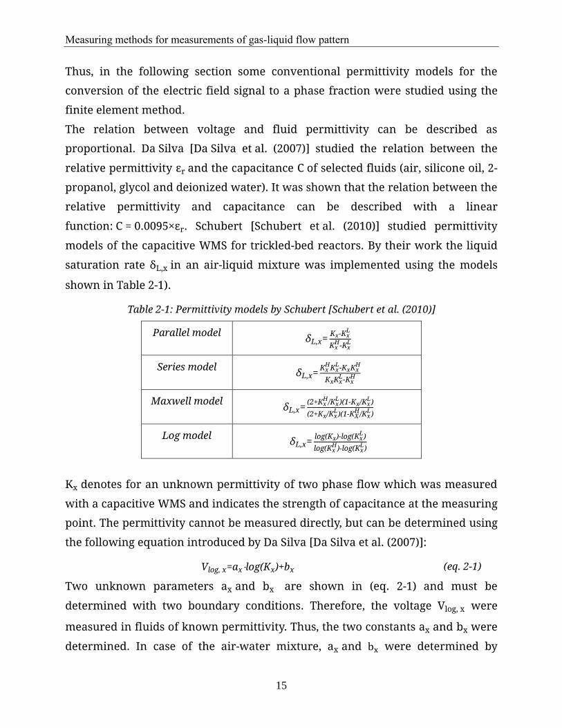
shown in Table 2-1).
Table 2-1: Permittivity models by Schubert [Schubert et al. (2010)]
Parallel model δL,x=
Kx-KxL
KxH-Kx
L
Series model δL,x=
KxHKx
L-KxKxH
KxKxL-Kx
H
Maxwell model δL,x=
(2+KxH/Kx
L)(1-Kx/KxL)
(2+Kx/KxL)(1-KX
H/Kx
L)
Log model δL,x=
log(Kx)-log(KxL)
log(KxH)-log(Kx
L)
Kx denotes for an unknown permittivity of two phase flow which was measured
with a capacitive WMS and indicates the strength of capacitance at the measuring
point. The permittivity cannot be measured directly, but can be determined using
the following equation introduced by Da Silva [Da Silva et al. (2007)]:
Vlog, x=ax⋅log(Kx)+bx (eq. 2-1)
Two unknown parameters ax and bx are shown in (eq. 2-1) and must be
determined with two boundary conditions. Therefore, the voltage Vlog, x were
measured in fluids of known permittivity. Thus, the two constants ax and bx were
determined. In case of the air-water mixture, ax and bx were determined by
Measuring methods for measurements of gas-liquid flow pattern
16
measuring the permittivity of water KxH as the medium of higher permittivity and
air 𝐾𝑥𝐿 , which has a lower permittivity. It should be noted that the values of ax and
bx depend not only on the relative permittivity but also on the temperature.
Furthermore, the signal noise can influence both parameters significantly.
Therefore, it is recommended to perform calibration measurements (for
determination of ax and bx) before and after each measurement using the
capacitive WMS.
The results presented by Schubert [Schubert et al. (2010)] for the determination of
the permittivity model for the trickle-bed reactor were validated with a liquid
collection method for local liquid flows. However, results generated by this method
were not representative, since the collection method measured flow rates, while
the capacitive WMS measured phase fractions in across the cross section.
Literature shows that it is necessary to understand the relation between measured
permittivity and the phase fraction more accurately. However, for the application
of the capacitive WMS used in packed columns, there is no existing theoretical
model yet. In this sense, the following sections are dealing with the influence of the
electric field on the phase distribution, studied with the commercial Software
ANSYS®
2.2.2.2 Parameters of the capacitive WMS
The WMS, which was delivered by Helmholz-Zentrum Rossendorf-Dresden, with
the diameter of 288 mm comprises two planes. In each plane there are 32 stainless-
steel wires of 0.2 mm in diameter and an equidistant spacing of 9.0 mm from each
other. The distance between the two planes (transmitter and receiver plane) is 3
mm and the wires from different planes are orthogonal to each other. The sensor
measures electrical signals (capacitance), if two wires from different planes are
activated. This arrangement results in a grid of 32×32 sensing points with a total of
1024 crossings of which 840are inside the circular cross section of the column. The
remaining 184 crossings are outside of the circular column cross-section. These
outer sensing points are masked out and thus they are not considered for the
measurements. The measuring frequency is set as 400 Hz (400 frames per second).

Measuring methods for measurements of gas-liquid flow pattern
17
Quasi-static time-harmonic electric (AC) condition is used for this electric field
simulation and the excitation frequency of the WMS is set as 10-5 Hz. For the
demodulation of the AC signals, a logarithmic detector scheme is used. Therefore,
the study of the electric field can be categorized as a low frequency electric field
problem. Dielectric changes are reflected in the measured voltage values. Due to
the fact, that many conductor wires are arranged within the cross section, the cross-
talk should be sufficiently suppressed by applying driver circuits. This leads to
limitations concerning the maximum conductivity of the liquid phase. The device
can work at liquid conductivities up to approximately 1000 μS/cm (tap water
quality). The lower limit is given by the sensitivity of the input cascades (0.1 μS/cm,
distillate water).
The permittivity of material is given by ϵ = ϵ0×ϵr, whereby ϵ0 (ϵ0 = 8.85 ×
10−12 V−1m−1) denotes the vacuum permittivity. The relative permittivity ranges of
air and water are shown in Table 2-2. Organic liquids have intermediate
permittivity values, for instance ϵr=2 for oil, ϵr=20 for 2-propanol.
Table 2-2: Dielectric constants of common materials
Material Temperature
[°C] Frequency
[Hz] Dielectric constant
air 20 3 × 10⁶ 1 water 20 low 80
Sensor wire 20 - 2000
The size and position of bubbles and droplets measured with capacitive WMS can
strongly affect the electric field. The averaged dielectric coefficient is different for
individual cases. The dielectric coefficient, depending on the medium capacitance,
can be calculated. The dependency of the capacitance measured with WMS can be
calculated by voltage (Calibration method). Finite element method (FEM)
simulation with ANSYS is used for the numerical electric field analysis.
2.2.2.3 Finite element method
Selection of finite elements using FEM is based on the freedom of element types,
e.g. element type Plane230 (quadrilateral, eight nodes, see Figure 2-9), which has
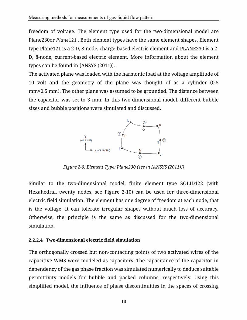
Measuring methods for measurements of gas-liquid flow pattern
18
freedom of voltage. The element type used for the two-dimensional model are
Plane230or 𝑃𝑙𝑎𝑛𝑒121 . Both element types have the same element shapes. Element
type Plane121 is a 2-D, 8-node, charge-based electric element and PLANE230 is a 2-
D, 8-node, current-based electric element. More information about the element
types can be found in [ANSYS (2011)].
The activated plane was loaded with the harmonic load at the voltage amplitude of
10 volt and the geometry of the plane was thought of as a cylinder (0.5
mm×0.5 mm). The other plane was assumed to be grounded. The distance between
the capacitor was set to 3 mm. In this two-dimensional model, different bubble
sizes and bubble positions were simulated and discussed.
Figure 2-9: Element Type: Plane230 (see in [ANSYS (2011)])
Similar to the two-dimensional model, finite element type SOLID122 (with
Hexahedral, twenty nodes, see Figure 2-10) can be used for three-dimensional
electric field simulation. The element has one degree of freedom at each node, that
is the voltage. It can tolerate irregular shapes without much loss of accuracy.
Otherwise, the principle is the same as discussed for the two-dimensional
simulation.
2.2.2.4 Two-dimensional electric field simulation
The orthogonally crossed but non-contacting points of two activated wires of the
capacitive WMS were modeled as capacitors. The capacitance of the capacitor in
dependency of the gas phase fraction was simulated numerically to deduce suitable
permittivity models for bubble and packed columns, respectively. Using this
simplified model, the influence of phase discontinuities in the spaces of crossing

Measuring methods for measurements of gas-liquid flow pattern
19
points can be analyzed in two dimensions. In addition, the electric field between
two wires of WMS was extended to a three-dimensional field. The three-
dimensional models were applied to study the influence of phase discontinuities in
the scenarios: the bubbles/droplets are not exactly located in the center between
two activated wires.
Figure 2-10: Element Type: Solid122 (see in [ANSYS (2011)])
The two-dimensional simulation model is shown in Figure 2-11. The range drawn
with depicted lines is concerned in the electric field simulation.
Figure 2-11: Two-dimensional geometry for electric field simulation
For this two-dimensional model, the orthogonally crossed points of activated and
Measuring methods for measurements of gas-liquid flow pattern
20
grounded wires are assumed as capacitors. This simplification aims to study the
influence of the phase distribution on the simulated capacitance. The length of the
activated wires can influence the simulated capacitance and is studied using the
three-dimensional electric field simulation.
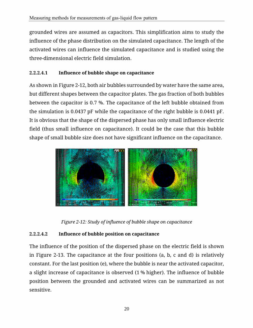
2.2.2.4.1 Influence of bubble shape on capacitance
As shown in Figure 2-12, both air bubbles surrounded by water have the same area,
but different shapes between the capacitor plates. The gas fraction of both bubbles
between the capacitor is 0.7 %. The capacitance of the left bubble obtained from
the simulation is 0.0437 pF while the capacitance of the right bubble is 0.0441 pF.
It is obvious that the shape of the dispersed phase has only small influence electric
field (thus small influence on capacitance). It could be the case that this bubble
shape of small bubble size does not have significant influence on the capacitance.
Figure 2-12: Study of influence of bubble shape on capacitance
2.2.2.4.2 Influence of bubble position on capacitance
The influence of the position of the dispersed phase on the electric field is shown
in Figure 2-13. The capacitance at the four positions (a, b, c and d) is relatively
constant. For the last position (e), where the bubble is near the activated capacitor,
a slight increase of capacitance is observed (1 % higher). The influence of bubble
position between the grounded and activated wires can be summarized as not
sensitive.

Measuring methods for measurements of gas-liquid flow pattern
21
Figure 2-13: Study of influence of bubble position on capacitance
2.2.2.4.3 Influence of bubble fraction on capacitance
From the previous results, it is known that the position and shape of dispersed
phase has almost no influence on the total capacitance. Nevertheless, the gas
fraction between the capacitor plates can influence the capacitance. To study the
influence of gas phase on the capacitance, the gas fraction is varied.
Figure 2-14: Study of influence of bubble holdup on capacitance
gas phase
water phase
activated wire
grounded wire a b c d e
activated wire
grounded wire
gas phase
water phase

Measuring methods for measurements of gas-liquid flow pattern
22
As shown in Figure 2-14, the gas fraction varies from 12 % to 93.4 %. Blue areas
denote for the liquid phase while the green area represent the gas phase. Relation
between gas fraction and capacitance was studied and results are illustrated in
Figure 2-15. It is clear that the gas fraction significantly influences the electric field
and the relation between capacitance and gas fraction in the entire range of the
capacitor for the bubble column can be fitted by a linear function.
Figure 2-15: Dependency of simulated capacitance on gas fraction
At lower gas fractions (up to 10 %), the capacitance changes relatively sensitive to
an increase of the gas fraction. With increasing gas fraction, the sensitivity of
capacitance is reduced. The relation between capacitance and phase fraction over
the entire range of gas fractions (from 0 % to 100 %) can be approximated as a
linear function.
The previously discussed procedure and analysis of gas bubbles can be extended
for the case of dispersed liquid phase and the continuous gas phase is gas, e. g.
droplets in a packed column. The influence of phase fraction on capacitance for
bubbles as dispersed phase (e.g. bubble column) and liquid as dispersed phase (e.g.

Measuring methods for measurements of gas-liquid flow pattern
23
packed column) are summarized in Figure 2-16.
It is shown that the dependency of capacitance on gas fraction in bubble columns
is approximately linear (blue curve with rectangular symbol) and the dependency
of capacitance in packed column is strongly non-linear (black curve with circle
symbol).
Fraction of dispersed phase
Relative permittivity of liquid phase is 5 (e.g. organic solution)
Figure 2-16: Dependency of normalized capacitance on phase holdup in bubble columns and packed columns
It is observed that for a relatively low liquid holdup and the change of capacitance
is relatively insensitive to the change of liquid holdup. That means, a small change
of measured or calculated capacitance could mean a large change of liquid holdup.
At relatively high liquid holdup, the capacitance is more sensitive to liquid holdup.
These results indicate that measurements with capacitive WMS have higher
accuracy for bubble columns than for packed columns. The relations of phase
fraction and permittivity for both applications are not identical.
Measuring methods for measurements of gas-liquid flow pattern
24
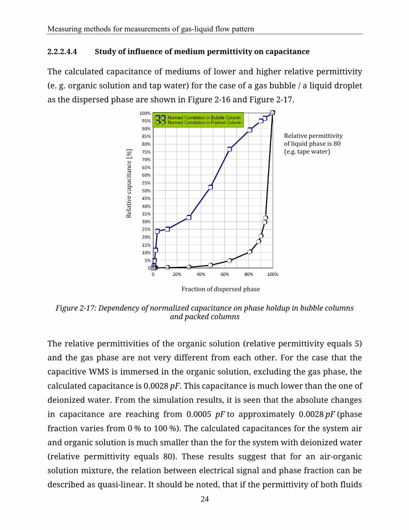
2.2.2.4.4 Study of influence of medium permittivity on capacitance
The calculated capacitance of mediums of lower and higher relative permittivity
(e. g. organic solution and tap water) for the case of a gas bubble / a liquid droplet
as the dispersed phase are shown in Figure 2-16 and Figure 2-17.
Fraction of dispersed phase
Relative permittivity of liquid phase is 80 (e.g. tape water)
Figure 2-17: Dependency of normalized capacitance on phase holdup in bubble columns and packed columns
The relative permittivities of the organic solution (relative permittivity equals 5)
and the gas phase are not very different from each other. For the case that the
capacitive WMS is immersed in the organic solution, excluding the gas phase, the
calculated capacitance is 0.0028 pF. This capacitance is much lower than the one of
deionized water. From the simulation results, it is seen that the absolute changes
in capacitance are reaching from 0.0005 pF to approximately 0.0028 pF (phase
fraction varies from 0 % to 100 %). The calculated capacitances for the system air
and organic solution is much smaller than the for the system with deionized water
(relative permittivity equals 80). These results suggest that for an air-organic
solution mixture, the relation between electrical signal and phase fraction can be
described as quasi-linear. It should be noted, that if the permittivity of both fluids

Measuring methods for measurements of gas-liquid flow pattern
25
not significantly differs from each other, this could make measurements less
accurate.
2.2.2.5 Three-dimensional electric field simulation
As shown in Figure 2-18, gas bubbles with different radiuses which are located on
the crossing point of the WMS were studied using the three-dimensional electric
field simulation. The activated and grounded wire are marked in red. The
dispersed phase is a gas bubble which is surrounded by a liquid phase (e. g.,
deionized water). The diameter of the dispersed bubble was varied to investigate
its influence on capacitance.
2.2.2.5.1 Influence of bubble size on capacitance
Capacitance was calculated for various bubble sizes. In Figure 2-19 it is shown that
the bubble size has a strong influence on the sum of electrical flux density vectors.
Gas bubbles were assumed as spheres to focus on the influence of capacitance on
bubble size. One can certainly assume other types of dispersed bubble shapes, but
as previously discussed, the two-dimensional simulation shows that the influence
of bubble shape can be neglected with acceptable small errors. Following, the
bubble size up to 4 mm was studied. The dependency of bubble radius on
capacitance can be described by a linear function (from bubble size of 0.9 mm to
Figure 2-18: Three-dimensional geometry of the electric field simulation
activated wire
grounded wire
neighbored wires
Disperse phase (droplet or bubble)

Measuring methods for measurements of gas-liquid flow pattern
26
4 mm) as shown in Figure 2-19.
It is observed that, although the orthogonally crossing point of the activated and
grounded wire is enclosed by a large bubble, the simulated capacitance is larger
than the capacitance of single continuous gas phase. The capacitance has merely
reached 50 % of the capacitance difference between pure water and pure gas
phase. This is since the part of wires near the crossing point still have strong
influence on capacitance. This three-dimensional simulation shows that the
capacitance also has a linear dependency on the bubble radius.
Figure 2-19: Influence of bubble size on capacitance (left Figure shows the electric field simulation; the right Figure shows the dependency of capacitance on bubble size based on
the results of electric field simulation)
2.2.2.5.2 Influence of bubble position (in contact to wires) on capacitance
As shown in Figure 2-20, the influence of decentral (from the crossing point) bubble
positions, that are still in contact with either the activated or the grounded wire by
various positions of bubbles (∅ = 2 mm), were studied.
It is shown that by the variation of bubble positions on the wire the absolute
changes of capacitance are significant. The variation of capacitance in this case
ranges from 12.65 pF to 11.9 pF. The sensitivity of a bubble can consider to be

Measuring methods for measurements of gas-liquid flow pattern
27
(12.65 pF - 11.9 pF) / 11.9 pF =10 %. As previously discussed, the bubble size at the
cross point has a stronger influence.
2.2.2.5.3 Influence of bubble position (without contact to wires) on capacitance
In the previous case was assumed that the bubble is in contact with the wires.
However, even small bubbles could flow through the WMS without touching the
wires. Therefore, the sensitivity of small bubbles without and with contact to the
activated wires were investigated.
Figure 2-20: Influence of bubble position on capacitance (left Figure shows the electric field simulation; the right Figure shows the dependency of capacitance on bubble
position based on the results of electric field simulation)
Given the case, that the rising bubble (∅ = 2 mm) has not touched the wire yet, the
bubble towards the wire (shown in Figure 2-21) was simulated. The electrical flux
density was influenced by the bubble, even at a distance of 4.5 mm to the crossing
point (shown in the first row). Distance variations from up to 4.5 mm from the
activated wires were studied. The bubble in contact with the wire at different
position has a more significant influence on capacitance compared to the bubble
without wire contact. The bubble which is not touching the wires has still influence
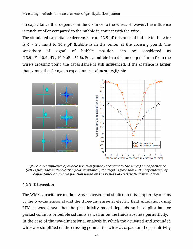
Measuring methods for measurements of gas-liquid flow pattern
28
on capacitance that depends on the distance to the wires. However, the influence
is much smaller compared to the bubble in contact with the wire.
The simulated capacitance decreases from 13.9 pF (distance of bubble to the wire
is ∅ = 2.5 mm) to 10.9 pF (bubble is in the center at the crossing point). The
sensitivity of signal of bubble position can be considered as
(13.9 pF - 10.9 pF) / 10.9 pF = 29 %. For a bubble in a distance up to 1 mm from the
wire’s crossing point, the capacitance is still influenced. If the distance is larger
than 2 mm, the change in capacitance is almost negligible.
Figure 2-21: Influence of bubble position (without contact to the wires) on capacitance (left Figure shows the electric field simulation; the right Figure shows the dependency of
capacitance on bubble position based on the results of electric field simulation)
2.2.3 Discussion
The WMS capacitance method was reviewed and studied in this chapter. By means
of the two-dimensional and the three-dimensional electric field simulation using
FEM, it was shown that the permittivity model depends on its application for
packed columns or bubble columns as well as on the fluids absolute permittivity.
In the case of the two-dimensional analysis in which the activated and grounded
wires are simplified on the crossing point of the wires as capacitor, the permittivity

Measuring methods for measurements of gas-liquid flow pattern
29
models for both, bubble columns and packed columns, respectively, can be derived.
The relative permittivity of the medium can also strongly influence the permittivity
models.
For the three-dimensional model, analysis is more complicated due to the large
possibility of bubble positions and sizes. It is not possible to consider all scenarios
to derive a unique permittivity model for both, bubble and packed columns.
In the simulation studies it is found that the capacitance depends on the bubble
diameter quasi-linear. Moreover, it is shown that the bubble size and bubble
position have strong influence on the measured signals. The bubbles which flow
through the wires without contact are still measurable up to certain distance. In
other words, total phase fraction of very small bubbles could be underestimated
and of large bubbles will be measured more accurate according to these simulation
results.
By an increase of wire number, the spatial resolution can be certainly improved.
However, the intrusiveness will increase significantly as well. In this study, it was
shown that the application of this method is suitable for multiphase measurements
with acceptable accuracy.
2.3 Measurements of bubble rise velocity and bubble size using
optical fiber method
The optical fiber method was studied by Miller [Miller and Mitchie (1970)] to
measure bubbles in a two-phase flow. Fordham [Fordham et al. (1999)] studied the
factors that influenced the accuracy of measurements by comparison of cross-
sectional profiles across the pipe diameter and time-averaged volume fractions of
a liquid-liquid flow. It was shown that surface treatments influenced the accuracy
of measurements strongly. Fordham [Fordham et al. (1999)] studied the application
of the optical method in kerosene/air and crude oil/nitrogen flows. The bubble
profile was successfully measured using this method.
2.3.1 Single optical fiber method
Vejrazka [Vejrazka et al. (2010)] studied isolated bubbles freely rising in a still

Measuring methods for measurements of gas-liquid flow pattern
30
liquid. The intrusiveness of the optical method was studied by comparison of the
dwell time of the probe tip within the gas phase and the expected value for a non-
perturbed bubble. It was noted that the interaction increased the dwell time and
the local void fraction was underestimated. However, the void fraction error can
be correlated with a modified Weber number. Bubble velocity and bubble diameter
were measured with a single tip optical probe in a bubble column by Mizushima
[Mizushima et al. (2013)]. The position and angle between the tip and the measured
bubble were not clearly determined. A pre-signal which was analyzed using a
three-dimensional computational ray tracing method was applied. The simulator
traced enormous ray segment trajectories in an optical fiber and rendered
complicated optical boundary conditions. Evaluation of the complex output signals
were achieved by computing the polarization and energy of every ray. On this way,
the image quality was improved.
2.3.2 Four optical fiber method
The four-point optical method studied by Guet [Guet et al. (2005)] was validated
using image analysis. A new algorithm was developed for the evaluation of the
four-point optical fiber method to estimate bubble orientation and shape. It was
also suggested to analyze bubble orientation and shape in more detail and for
multiple bubble shear flow. Xue [Xue et al. (2008)] used the four-point optical fiber
method in a cylindrical bubble column with a diameter of 16.2 cm. The bubble
velocity and size in bubbly and highly churn turbulent flow were determined.
2.3.3 Double optical fiber method
Saberi [Saberi et al. (1995)] developed a method to detect and measure bubble sizes
and velocities in a gas-liquid column. Bubble velocity was calculated using two
identical parallel fibers and the cross-correlation technique. With the velocities and
the passage time determined, it was possible to determine the bubble diameter. The
double tip fiber probe method was used by Kiambi [Kiambi et al. (2001)]. They
determined the time averaged local interfacial area in a riser of an airlift reactor
for an air/water medium. The dimensions of the riser were 0.094 m in diameter and

Measuring methods for measurements of gas-liquid flow pattern
31
1.2 m in height. Both optical probes had a distance of 3.2 mm. Chaumat [Chaumat
et al. (2005)] also used a double tip optical probe technique in a rectangular tank.
They tested the reliability of the probe data with a high-speed camera. The shape
and velocity of even distorted and tumbling bubbles were studied. Chaumat
[Chaumat et al. (2007)] extended the double fiber probe for more complex flow in
a bubble column with a diameter of 0.2 m. Rüdisüli [Rüdisüli et al. (2012)] used the
double tip optical fiber method to measure the bubble size and bubble rise velocity
in fluidized beds. A bubble linking algorithm based on regression techniques was
proposed. Due to slugging and wall effects, the bubble rise velocity did not show a
clear trend that an increased gas velocity and an elevated probe height lead to
larger bubbles and a modified bubble size distribution.
2.3.4 Laser doppler anemometer
Laser doppler anemometer (LDA) in bubble columns were basically explained and
discussed by Gross [Gross (1990)]. Kulkarni [Kulkarni (2005)] applied the LDA
method to study the influence of flow patterns of single point sparger on the local
flow field in a bubble column. Therning [Therning and Rasmuson (2005)] measured
liquid velocities in a small-scale bubble column with an internal diameter of
50 mm, packed with glass Raschig rings of 10 and 15 mm. It was found that the axial
time-averaged liquid velocity was lower than that obtained in empty bubble
columns. Although this method was non-intrusive, the application was limited to a
relative low gas holdup, and the bubbles close to the center of the bubble column
were not accurately measurable at higher gas loads.
2.3.5 Particle image velocimetry
Particle image velocimetry (PIV) was used by Chaouki [Chaouki et al. (1997)] in gas-
liquid flow to determine either the liquid velocity or the bubble velocity and size.
This method is advantageous to clearly investigate the fluid hydrodynamics.
Images were captured using a digital camera with a charge-coupled device (CCD)
chip. Delnoij [Delnoij et al. (1999)] reviewed the basic applications of the PIV
method in bubble columns and introduced some new points considering gas and

Measuring methods for measurements of gas-liquid flow pattern
32
liquid flow fields induced by a bubble plume rising in a rectangular bubble column.
Nevertheless, the addition of small particles which flow with the gas and liquid
influences the original process condition.
2.3.6 Optical fiber method
An experimental method using the double optical fiber method described by Ji [Ji
(2007)] was employed in this work for the measurement of the bubble rise velocity
and the bubble size in a bubble column (∅ = 288 mm). Experimental equipment
(Laser Doppler and high-speed camera) were supplied by Prof. Walzel from
University Dortmund. The method suggested by Saberi [Saberi et al. (1995)] (cross-
correlation method) for data processing using the software MATLAB® has been
applied in this work to analyze the bubble size and bubble rise velocity.
The measuring system consisted of multiple light-guide fibers with a step-index
profile, wherein the fiber core material was Polymethylmethacrylate (PMMA). An
important feature of the fibers used in this work is the relatively large fiber core
diameter of 490 μm. The large fiber core is favorable for an in-line light coupling.
The concept of the optical fiber method exploited the Fresnel-effect on the interface
between a fiber tip and the surrounding fluid, which can be either a gas phase or a
liquid phase. When light was coupled into the fiber on one side, the intensity of the
reflected light on the other end depended on the refractive index difference
between the fiber core material and the fiber environment. The intensity of the
reflected light reached its minimum when the refractive index of the fiber core
material and the surrounding fluid was almost equal. With increasing difference
in refractive index, the intensity of the reflected light increased. Applying this
principle to the multi-phase flow within a bubble column, where one fluid was air
(nA = 1) and the other was water (nW = 1.33), the maximum intensity was achieved
when the fiber tip was located within a moving bubble. For other cases, i.e. when
the fiber tip was surrounded by water, the intensity of the reflected light was
reduced. Mounting a CCD element on the opposing end of the fiber, the local phase
changes on the fiber tip within the multiphase flow were visualized as a light
intensity plot over time.
Measuring methods for measurements of gas-liquid flow pattern
33
Since both sides of the fibers were used in the present configuration, the light
coupling had to be achieved in-line. An additional challenge was that the major
amount of the light was coupled in the direction of the sensor tip, as it otherwise
would blend the measuring signal on the receiving side of the fiber.
The procedure of light coupling was performed through laser diode. A laser diode
with a power of 1 W and a wavelength of 660 nm was used along with a CCD line
scan camera with a sampling rate of 33.7 kHz. The advantage of this set-up is the
possibility to realize a light coupling into multiple fibers with relatively low
equipment requirements. A laser line with a flat-top intensity profile was generated
using a laser-diode and a proper lens configuration. A flat-top profile was needed
to ensure that the same amount of light was coupled in each fiber, leading to a
comparable signal quality for all sensor fibers. To achieve a selective light coupling
in the preferred direction, a bending coupler was used. The bending coupler was a
massive wedge, where one or multiple fibers were bend along its sharp edge. Due
to the bending, the fibers become permeable to light. Realizing a proper
arrangement of both, the laser-diode and the wedge, most of the light can be
coupled in the measuring direction.

Study of phase distribution in bubble columns
34
3 Study of phase distribution in bubble columns
Bubble columns are widely used as gas-liquid contacting apparatuses in the
chemical, biochemical and petrochemical industry. The gaseous phase in form of
bubbles is brought in contact with the liquid phase. Compared to other chemical
reactors, bubble columns have excellent heat and mass transfer characteristics -
high heat and mass transfer coefficients. Little maintenance and low operating
costs are required. Although the construction of bubble columns is simple, the
hydrodynamics of bubble columns are complex. Therefore, it is essential to apply
reliable measurement methods for the study of hydrodynamics in bubble columns
with high temporal and spatial resolution.
3.1 Flow regime in bubble columns
The disperse phase of bubble column is the gas phase while liquid phase is
continuous. As a bubble rises upwards in bubble columns, the movement speed in
axial direction is defined as axial velocity. Fluctuations of bubbles causes an
additional radial velocity. Flow regimes of bubbles in bubble columns can be
categorized as homogeneous regime, transition regime and heterogeneous regime,
depending on the superficial gas velocity and diameter of the bubble column.
The dependency of flow regime on the superficial gas velocity and diameter of the
bubble column is illustrated in Figure 3-1. In the homogeneous flow regime, it can
be assumed that the sizes of bubbles are equal. In the heterogeneous flow regime
bubble clusters of mixed different bubble sizes are formed. The flow regimes of
bubbles in a bubble column are dependent on design parameters (e.g. distributor
design, column diameter), operating parameters (e.g. superficial gas and liquid
velocities) and physical properties (viscosity, surface tension, density and
coalescing nature of the liquid phase).
In the homogeneous flow regime, the gas holdup increases markedly with the
superficial gas velocity. The bubble size is roughly uniform and the radial profile
of gas holdup is nearly flat. This was validated by Euzen [Euzen, Jp. et al. (2000)].
The trajectory of a small bubble (1.12 mm) was experimentally studied and

Study of phase distribution in bubble columns
35
demonstrated by Shew [SHEW et al. (2006)]. At a low gas velocity range, the
distributor design affects gas holdup as reported by Luo [Luo et al. (1999)]. The
transition flow regime can be reached by increasing the superficial gas velocity
from the homogeneous regime. In the transition flow regime, larger bubbles can
be formed. Large bubbles move more quickly than small bubbles. This flow regime
is not as homogeneous as the homogeneous flow regime. The radial profile of gas
holdup shows a maximum at the center of the bubble column, and gas distribution
is nearly zero at the wall as reported by Krishna [Krishna et al. (1996)].
Figure 3-1: Flow regimes in bubble column reported by Deckwer
[Deckwer et al. (1980)]
In the heterogeneous flow regime, bubble coalescence and breakage are
significantly present. The breakage and coalescence mechanisms are responsible
for two classes of bubbles (Large and small bubbles). Liquid recirculation and
radial gas holdup profiles were studied by Chen [Chen et al. (2004)]. An increase of
the gas superficial velocity leads to a higher gas holdup. This slug flow regime is
highly unstable. The gas passes through the liquid as intermittent plugs, while the
liquid continuously pulsates up and down near the wall. However, the slug flow
regime is generally limited to columns of small diameter. The domain of industrial

Study of phase distribution in bubble columns
36
interest concerns in particular the heterogeneous regime, characterized by high
mass and heat transfers. Bubble columns were studied by Deckwer [Deckwer and
Field (1992)].
The capacitive WMS discussed in the previous chapter was applied for the study of
phase distribution in an air/water system. Since one WMS is not able to be used for
the determination of the bubble rise velocity, the application of two WMS is
necessary, which, however, will strongly influence the phase distribution. Large
bubbles can be cut by the wires in multiple bubbles after passing through the first
WMS. This bubble cannot be identified by the second WMS. For that reason, the
optical fiber method was applied as additional method for the study of the bubble
rise velocity.
3.2 Experimental measurements of bubble column
3.2.1 Measurements of bubble distribution using WMS
Phase distribution in a bubble column (∅ = 0.288 m) was studied with a WMS. The
working principle of the WSM was discussed previously. By the electric field
simulation of the WMS, it was seen that the electrical signals of WMS were
evaluated with a linear relation for the bubble fraction. In this chapter the
experimental measurements of bubble distribution in the bubble column with
capacitive WMS are presented and the results are discussed.
As shown in Figure 3-2, a bubble column (air/deionized water system) with a
constant diameter of 0.288 m was investigated.
The vertical distance between gas distributor and WMS was about 1 m. Gas phase
was distributed through two orthogonally crossed pipes with small holes of 2 mm
diameter. The gas phase flowed through the gas distributor from the bottom into
bubble column and left from the top of the bubble column. The liquid phase was
stationary, without further in and outlet streams. As the superficial gas velocity was
increased, the flow regime changed from the homogeneous flow regime over the
transition range to the heterogeneous flow regime (Figure 3-2). Phase distribution
at different superficial gas velocities (2 cm/s, 4.2 cm/s, 8.4 cm/s, 16.8 cm/s) was

Study of phase distribution in bubble columns
37
measured with the capacitive WMS.
Figure 3-2: Flow regimes in studied operating points of bubble column and experimental setup for phase distribution measurements using the WMS
3.2.1.1 Experimental results of the capacitive WMS
As shown in Figure 3-3, the spatial distribution of the gas phase (colored ranges) in
the cross-section of the bubble column was measured with a WMS. The colored
regions are indicating the gas phase while the white areas are representing the
liquid phase.
It was observed that at the moment of measurement the gas phase can be clearly
distinguished from the liquid phase due to the difference in permittivity. For this
process conditions (gas superficial velocity was 2 cm/s), the flow regime was
homogeneous. Figure 3-4 illustrates the phase distribution over time in intervals of
0.025 s. Due to bubbles changing their position continuously, it is important to study
the phase distribution over an integral time interval.
uG = 16.8 cm/s
uG = 2 cm/s
uG = 8.4 cm/s

Study of phase distribution in bubble columns
38
Figure 3-3: Gas phase distribution across the cross-section of a bubble column measured by
the WMS
At a superficial gas velocity of 8.4 cm/s a large bubble cluster was observed to pass
the WMS over a time interval of 112 ms as shown in Figure 3-4. Due to the high
temporal resolution, it can be seen, that the bubble cluster has a quite irregular
shape and within the cluster even some interfacial area was recognized between
50 and 70 ms.
Figure 3-4: Temporal distribution of bubble clusters in cross-section of bubble column

Study of phase distribution in bubble columns
39
A bubble flow profile of the transient regime is shown in Figure 3-5. The shown
phase distribution was taken along the diameter of the bubble column with time
intervals of 0.5 s. At a low superficial gas velocity of 2 cm/s the gas flow was mainly
bubble flow. Relatively large bubbles occurred primarily at the center of the
column while close to the wall there were almost no or too small bubbles to be
detected. With an increase of the superficial gas velocity the homogeneous bubble
flow (e.g. superficial gas velocity at 8.4 cm/s) turned to a mixed size bubble flow.
Larger bubbles were also found mostly near the center of the bubble column.
Smaller bubbles were detected near the wall. With a further increase of the
superficial gas velocity to 16.8 cm/s, large bubbles in forms of bubble clusters were
observed. The reason are the larger bubbles at the center of the bubble column that
raised much faster than the surrounding small bubbles. Due to circulation of the
liquid (downwards near the column wall and upwards in the center) the small
bubbles were transferred away from the wall into the center of the bubble column.
The small and large bubbles formed bubble clusters, where the interfacial area
cannot clearly be identified.
Figure 3-5: Temporal and spatial gas phase distribution at different operating points (flow regimes)
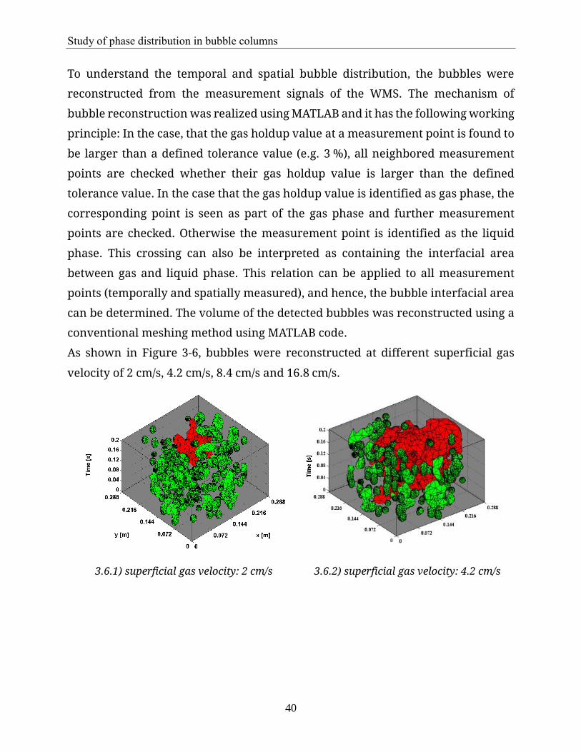
Study of phase distribution in bubble columns
40
To understand the temporal and spatial bubble distribution, the bubbles were
reconstructed from the measurement signals of the WMS. The mechanism of
bubble reconstruction was realized using MATLAB and it has the following working
principle: In the case, that the gas holdup value at a measurement point is found to
be larger than a defined tolerance value (e.g. 3 %), all neighbored measurement
points are checked whether their gas holdup value is larger than the defined
tolerance value. In the case that the gas holdup value is identified as gas phase, the
corresponding point is seen as part of the gas phase and further measurement
points are checked. Otherwise the measurement point is identified as the liquid
phase. This crossing can also be interpreted as containing the interfacial area
between gas and liquid phase. This relation can be applied to all measurement
points (temporally and spatially measured), and hence, the bubble interfacial area
can be determined. The volume of the detected bubbles was reconstructed using a
conventional meshing method using MATLAB code.
As shown in Figure 3-6, bubbles were reconstructed at different superficial gas
velocity of 2 cm/s, 4.2 cm/s, 8.4 cm/s and 16.8 cm/s.
3.6.1) superficial gas velocity: 2 cm/s 3.6.2) superficial gas velocity: 4.2 cm/s
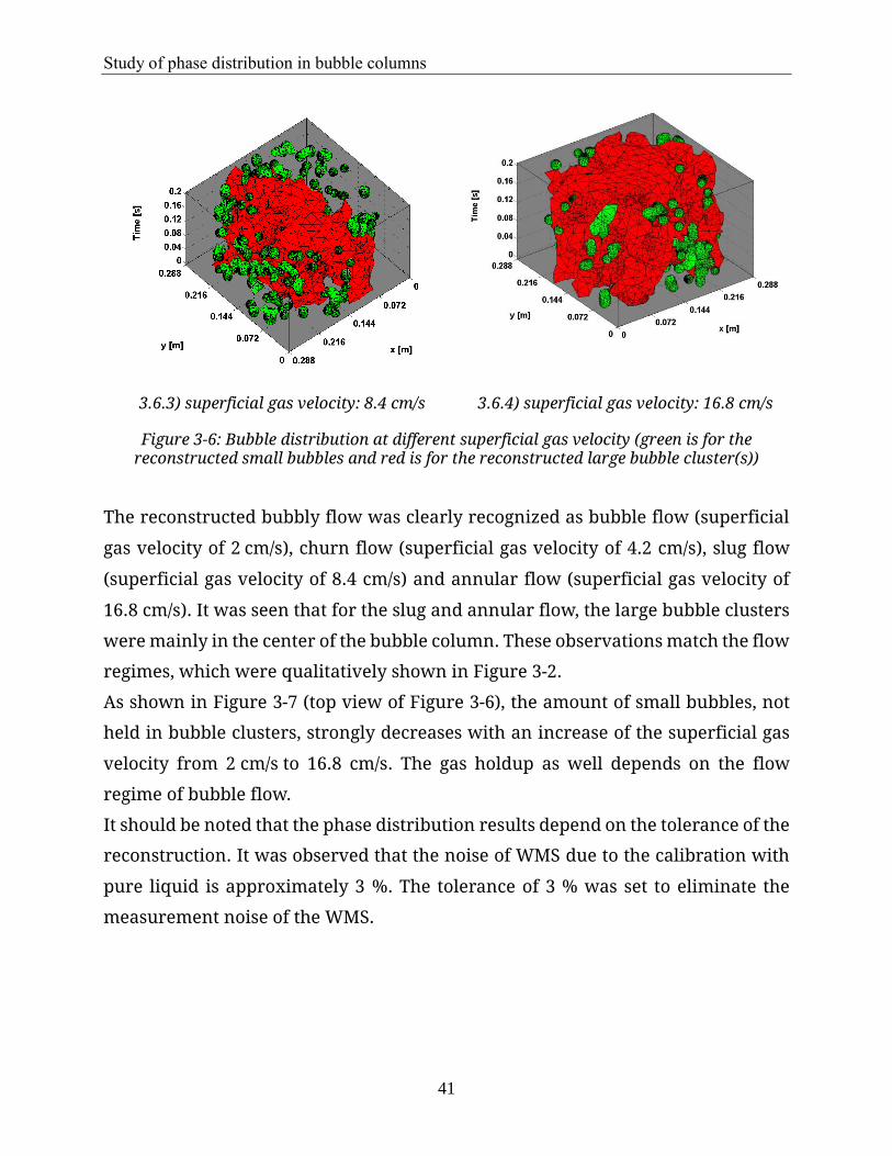
Study of phase distribution in bubble columns
41
3.6.3) superficial gas velocity: 8.4 cm/s 3.6.4) superficial gas velocity: 16.8 cm/s
Figure 3-6: Bubble distribution at different superficial gas velocity (green is for the reconstructed small bubbles and red is for the reconstructed large bubble cluster(s))
The reconstructed bubbly flow was clearly recognized as bubble flow (superficial
gas velocity of 2 cm/s), churn flow (superficial gas velocity of 4.2 cm/s), slug flow
(superficial gas velocity of 8.4 cm/s) and annular flow (superficial gas velocity of
16.8 cm/s). It was seen that for the slug and annular flow, the large bubble clusters
were mainly in the center of the bubble column. These observations match the flow
regimes, which were qualitatively shown in Figure 3-2.
As shown in Figure 3-7 (top view of Figure 3-6), the amount of small bubbles, not
held in bubble clusters, strongly decreases with an increase of the superficial gas
velocity from 2 cm/s to 16.8 cm/s. The gas holdup as well depends on the flow
regime of bubble flow.
It should be noted that the phase distribution results depend on the tolerance of the
reconstruction. It was observed that the noise of WMS due to the calibration with
pure liquid is approximately 3 %. The tolerance of 3 % was set to eliminate the
measurement noise of the WMS.

Study of phase distribution in bubble columns
42
3.7.1) superficial gas velocity: 2 cm/s 3.7.2) superficial gas velocity: 4.2 cm/s
3.7.3) superficial gas velocity: 8.4 cm/s 3.7.4) superficial gas velocity: 16.8 cm/s
Figure 3-7: Overview of bubble distribution at different superficial gas velocities (green is for the reconstructed small bubbles and red is for the reconstructed large bubble
cluster(s))
The local gas holdup in the radial direction (time- averaged) at a low superficial gas
velocity of 2 cm/s in Figure 3-8 and a high superficial gas velocity of 16.8 cm/s are
shown in Figure 3-9. At the low superficial gas velocity of 2 cm/s the gas holdup was
between 2 % and 5 % while at the higher superficial gas velocity of 16.8 cm/s, the
gas holdup within the center of the column cross section was much higher than the
one close to the wall (shown in Figure 3-10). Although the gas holdup at a superficial
gas velocity of 16.8 cm/s was high, it mainly occurred in form of large bubble
clusters. Compared to the small bubbles, large bubble clusters with the same gas
holdup have less interfacial area and a shorter residence time.

Study of phase distribution in bubble columns
43
Figure 3-8: Reconstructed profile for a superficial gas velocity of 2 cm/s
Figure 3-9: Reconstructed profile for a superficial gas velocity of 16.8 cm/s
Figure 3-10: Local radial gas holdup distribution
Comparison of gas holdups using the difference in height method and a WMS is
shown in Figure 3-11. It is shown that the gas holdup measured by the height
difference method is higher than the gas holdup that was measured with the WMS
for different superficial gas velocities. The reason might be small bubbles flowing
through the WMS without touching the wires. Hence, the number of small bubbles
measured with the WMS was underestimated.
Ga
s h
old
up
Column radius [m]
Tim
e [s
]
Tim
e [s
]
x coordinate [m] x coordinate
[m]
y coordinate [m]
y coordinate [m]

Study of phase distribution in bubble columns
44
Figure 3-11: Comparison of gas holdup measured with WMS and the height difference method
3.2.1.2 Conclusion
It was shown in this chapter that the capacitive WMS was successfully used for the
measurements of phase distribution in bubble columns. The high temporal
resolution of the WMS enables the detection of bubbles in ms. The high spatial
resolution of the WMS makes possible measurements of bubble distributions over
the whole cross section of a bubble column.
The measurements of flow regimes using the capacitive WMS have been validated
as qualitatively shown in Figure 3-2. Moreover, small and large bubbles (or bubble
clusters) could be distinguished in the measurements. It has been found that large
bubbles prefer to flow in the center of the bubble columns.
Gas holdups measured with capacitive WMS at different gas superficial velocities
were qualitatively similar to the measurements which were obtained with the
volume-averaged method (height difference method). Deviations of the results
between both methods were caused by the measuring principles of the WMS, by
which too small bubbles cannot be measured.
In summary, the capacitive WMS was applied successfully for the measurements of
phase distribution. It should be noted that, although the time interval of a large
Superficial gas velocity [cm/s]
Ga
s h
old
up

Study of phase distribution in bubble columns
45
bubble cluster can be measured, the bubble rise velocity is not measurable using
the WMS. Optical fiber methods were applied for the measurements of bubble rise
velocity in bubble columns.
3.2.2 Measurements of bubble rise velocity and bubble size using an optical
fiber method
3.2.2.1 Experimental setup
The main part of the experimental apparatus used for optical fiber method is a
cylindrical column (288 mm in diameter) that is shown in Figure 3-12. The positions
of the fibers and the corresponding distances are shown in Figure 3-13.
Figure 3-12: Bubble column equipped with the optical fiber
method
Figure 3-13: Schematic representation of the experimental setup using optical fibers in the bubble
column
Two fibers each were installed as a couple. The fibers were inserted into the bubble
column through sealed holes in the column wall. This method allows the
measurements of bubble rise velocity at 12 different positions. Each fiber couple
was inserted into a 20 cm long steel tube with 0.5 mm inner diameter to stabilize
the fibers. The length of the steel tube in the bubble column was varied over the
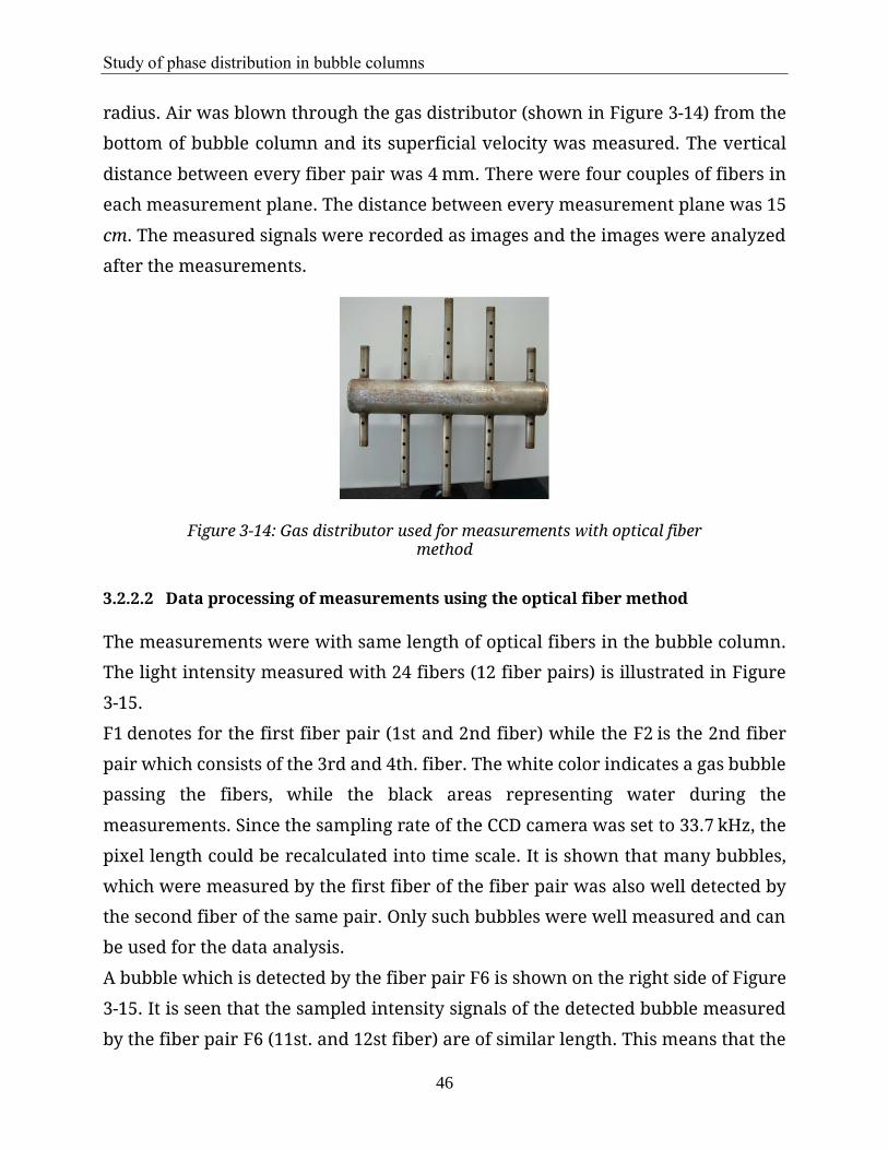
Study of phase distribution in bubble columns
46
radius. Air was blown through the gas distributor (shown in Figure 3-14) from the
bottom of bubble column and its superficial velocity was measured. The vertical
distance between every fiber pair was 4 mm. There were four couples of fibers in
each measurement plane. The distance between every measurement plane was 15
cm. The measured signals were recorded as images and the images were analyzed
after the measurements.
Figure 3-14: Gas distributor used for measurements with optical fiber method
3.2.2.2 Data processing of measurements using the optical fiber method
The measurements were with same length of optical fibers in the bubble column.
The light intensity measured with 24 fibers (12 fiber pairs) is illustrated in Figure
3-15.
F1 denotes for the first fiber pair (1st and 2nd fiber) while the F2 is the 2nd fiber
pair which consists of the 3rd and 4th. fiber. The white color indicates a gas bubble
passing the fibers, while the black areas representing water during the
measurements. Since the sampling rate of the CCD camera was set to 33.7 kHz, the
pixel length could be recalculated into time scale. It is shown that many bubbles,
which were measured by the first fiber of the fiber pair was also well detected by
the second fiber of the same pair. Only such bubbles were well measured and can
be used for the data analysis.
A bubble which is detected by the fiber pair F6 is shown on the right side of Figure
3-15. It is seen that the sampled intensity signals of the detected bubble measured
by the fiber pair F6 (11st. and 12st fiber) are of similar length. This means that the
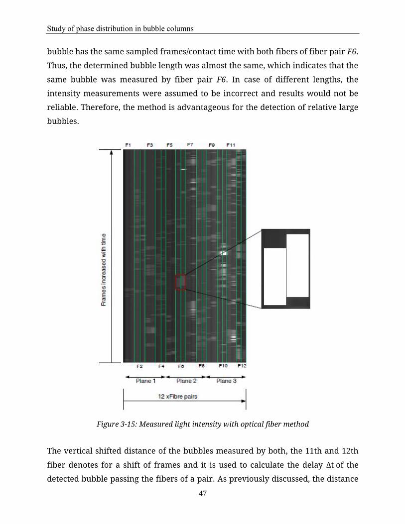
Study of phase distribution in bubble columns
47
bubble has the same sampled frames/contact time with both fibers of fiber pair F6.
Thus, the determined bubble length was almost the same, which indicates that the
same bubble was measured by fiber pair F6. In case of different lengths, the
intensity measurements were assumed to be incorrect and results would not be
reliable. Therefore, the method is advantageous for the detection of relative large
bubbles.
Figure 3-15: Measured light intensity with optical fiber method
The vertical shifted distance of the bubbles measured by both, the 11th and 12th
fiber denotes for a shift of frames and it is used to calculate the delay Δt of the
detected bubble passing the fibers of a pair. As previously discussed, the distance

Study of phase distribution in bubble columns
48
of the fiber pairs L is known and the time difference Δt from the first to the second
fiber can be calculated. Thus, the bubble rise velocity vb can be calculated using
(eq. 3-1).
vb=L
Δt
(eq. 3-1)
To obtain the time difference between two signals, the intensity signals of an 8-bit
monochrome image were analyzed using MATLAB®. Each intensity signal can be
represented over time. Since the noise of intensity signals influences the Δt,a
proper data processing has to be applied.
Figure 3-16: Calculation of time delay using cross-correlation used by Ji [Ji (2007)]
A well-known analysis method, namely the cross-correlation function applied by
Kipphan [Kipphan (1977)] and Ji [Ji (2007)], as shown Figure 3-16, was used for the
determination of the time difference. The correlation coefficient Ψxy(𝜏) was
determined from two signals x(t) and y(t) for each sensor pair:
ψxy
=1/T ∫ x(t-τ)⋅y(t)dt
T
0
(eq. 3-2)
In
(eq. 3-2), τ is the initial time difference and T is the considered period of time. If a
maximum of correlation coefficient ψxy(τ) is found, τ is the time difference to be
determined. It should be noted that ψxy(τ) can always be found mathematically
within a given range of τ . Therefore, it is necessary to verify whether the results
are reasonable.

Study of phase distribution in bubble columns
49
3.2.2.3 Experimental measurements of bubble rise velocity using the optical fiber
method
Bubble size and rise velocity at various positions of the bubble column radius and
superficial velocities were studied using the optical fiber method. The measured
intensities of each experiment are shown in Figure 3-17.
r/R=0.7
r/R=0.8
r/R=0.9
Figure 3-17: Experimental results at gas superficial velocity from 1.28 to 12.8 cm/s at r/R = 0.7, 0.8 and 0.9
As shown in Figure 3-18, the intensity at the front tips of the optical fibers were
measured within 1200 ms for the superficial gas velocity of 12.8 cm/s and a
dimensionless radius of 0.9 from the sensor position to the bubble column center.
Each peak of intensity denotes the detection of a bubble at the front tip of the optical
fiber.
On the one hand, some peaks were only measured by one of the two coupled
sensors, but not by the other one. On the other hand, the form of the bubble
measured by sensor 1 and 2 differed significantly from each other. Such bubbles
cannot be applied for analysis with the methods discussed.
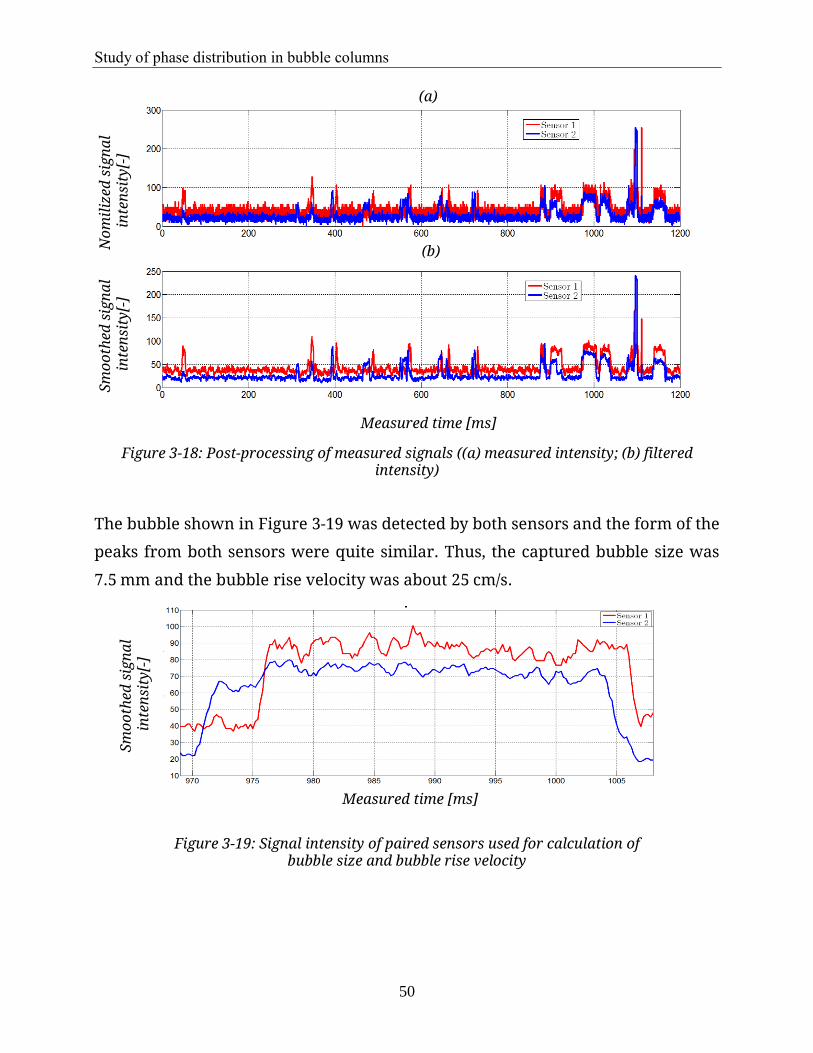
Study of phase distribution in bubble columns
50
Figure 3-18: Post-processing of measured signals ((a) measured intensity; (b) filtered intensity)
The bubble shown in Figure 3-19 was detected by both sensors and the form of the
peaks from both sensors were quite similar. Thus, the captured bubble size was
7.5 mm and the bubble rise velocity was about 25 cm/s.
Figure 3-19: Signal intensity of paired sensors used for calculation of bubble size and bubble rise velocity
Measured time [ms]
(a)
(b)
Measured time [ms]
No
mil
ized
sig
na
l i
nte
nsi
ty[-
] S
mo
oth
ed s
ign
al
in
ten
sity
[-]
Sm
oo
thed
sig
na
l i
nte
nsi
ty[-
]
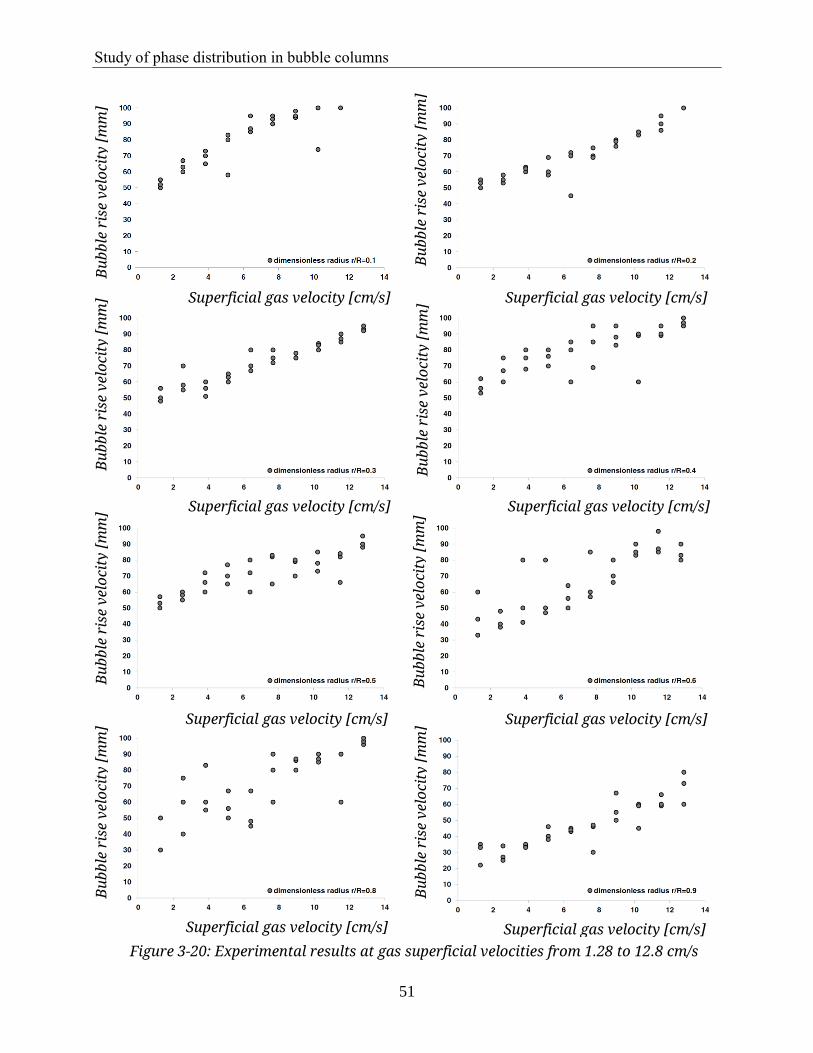
Study of phase distribution in bubble columns
51
Figure 3-20: Experimental results at gas superficial velocities from 1.28 to 12.8 cm/s
Superficial gas velocity [cm/s] Superficial gas velocity [cm/s]
Bu
bb
le r
ise
vel
oci
ty [
mm
]
Bu
bb
le r
ise
vel
oci
ty [
mm
] B
ub
ble
ris
e v
elo
city
[m
m]
Bu
bb
le r
ise
vel
oci
ty [
mm
]
Superficial gas velocity [cm/s] Superficial gas velocity [cm/s]
Bu
bb
le r
ise
vel
oci
ty [
mm
] B
ub
ble
ris
e v
elo
city
[m
m]
Superficial gas velocity [cm/s] Superficial gas velocity [cm/s]
Superficial gas velocity [cm/s] Superficial gas velocity [cm/s]
Bu
bb
le r
ise
vel
oci
ty [
mm
] B
ub
ble
ris
e v
elo
city
[m
m]

Study of phase distribution in bubble columns
52
The bubble rise velocity depending on superficial gas velocity and the
dimensionless radius of the bubble column is illustrated in Figure 3-20. The bubble
rise velocity is displayed at dimensionless radiuses of r/R = 0.1, 0.2, 0.3, 0.4, 0.5, 0.6,
0.8 and 0.9. The superficial gas velocity varies from 1.28 cm/s to 12.8 cm/s.
It is observed that with an increase in superficial gas velocity, the bubble rise
velocity increases from 50 cm/s to 100 cm/s, respectively. The variation of the
measured bubble rise velocity from r/R = 0.1 to 0.5 was not considerable. From a
dimensionless radius of r/R = 0.6, a slight decrease of bubble rise velocity at low
superficial gas velocities was observed, while that at higher superficial velocities is
still approximately 90 cm/s. At a dimensionless radius of r/R = 0.8 and 0.9, the
bubble rise velocity depends on the superficial gas velocity. The bubble rise velocity
at r/R = 0.9 is considerably smaller than the one in the middle range. It was
observed that the liquid near the column wall slightly circulated downwards. This
could result in a slowdown of the rising bubble flow, so that reasonable smaller
bubble rise velocities were observed.
The bubble rise velocity shown in Figure 3-21 at r/R = 0.7 was almost independent
of the superficial gas velocity. The reason of this phenomena could be that at this
dimensionless radius the bubbles flowing upwards are affected by the liquid phase
flowing downwards (circulation of liquid phase), so that the bubble rise velocities
were similar for different superficial gas velocities.
Figure 3-21: Experimental results at gas superficial velocities from 1.28 to 12.8 cm/s
Superficial gas velocity [cm/s]
Bu
bb
le r
ise
vel
oci
ty [
cm/s
] [m
m]

Study of phase distribution in bubble columns
53
Based on the data processing method (cross-correlation method) discussed earlier
in this chapter, the bubble diameters in dependence of superficial gas velocity and
dimensionless radius in the bubble column were also studied. The results are
shown in Figure 3-22.
Figure 3-22: Bubble size distribution in radial direction
It is seen that at a superficial gas velocity of 1.28 cm/s, the vertical bubble lengths
(assumed as bubble diameter) were approximately similar over the dimensionless
radius from 0.1 to 0.9. The measurements match the prediction that at this
superficial gas velocity the flow regime was approximately homogeneous.
Figure 3-23: Comparison of experimental results with data published
by Wallis [Wallis (1969)]
Superficial gas velocity: 12.8 [cm/s]
Superficial gas velocity: 1.28 [cm/s]
Superficial gas velocity: 6.4 [cm/s]
Dimensionless radius r/R [-]
Bu
bb
le d
iam
eter
[m
m]

Study of phase distribution in bubble columns
54
With an increase of superficial gas velocity to 6.4 cm/s and 12.8 cm/s, larger bubbles
were detected. It was seen that the higher the superficial velocity is, the larger is
the bubble diameter. Larger bubbles were mainly detected in the center of the
bubble column. Near the column wall only small bubbles were detected for the
studied superficial gas velocities. As it was shown by the measurements with
capacitive WMS, the flow regime was heterogeneous at a superficial gas velocity of
12.8 cm/s.
The comparison of the experimental results with literature shows a generally
higher bubble rise velocity for the studied bubble sizes of 2 mm to about 30 mm.
The reason could be that the optical fibers only measure parts of the larger bubbles,
so that the bubble rise velocity of a larger bubble is underestimated. Similar results,
as shown in Figure 3-24, were reported by Chaumat [Chaumat et al. (2005)], as well.
Figure 3-24: Experimental measurements of bubble rise velocities using an optical method by Chaumat [Chaumat et al. (2005)]
3.3 Conclusion
The optical fiber method was reviewed and studied in this chapter. It was shown
that the optical fiber method can experimentally be applied for the measurement
of gas-liquid flow (air-water) in bubble columns. Bubble rise velocities and bubble
sizes in axial direction were successfully measured. However, the analysis of
measured intensity signals should be handled with care. Only well measured
bubble signals can be considered for analysis. This method can be categorized as a
Axial bubble velocity [m/s]
Eq
uiv
ale
nt
dia
met
er [
mm
]

Study of phase distribution in bubble columns
55
pointwise method whereby the measurements depend significantly on the local
flow conditions.
Compared to other conventional experimental methods, measurements in bubble
columns with capacitive WMS and the optical fiber method, as shown in this work,
are low-intrusive. Thus, they only little affect the process hydrodynamics.
Compared to non-intrusive methods used for measurements in bubble columns,
the WMS has a higher spatial and temporal resolution while the optical fiber
method has only a high temporal resolution and can be used in the bubble column
on arbitrary positions. The limitation of both methods is the relatively complicated
data processing.

Study of phase distribution in packed columns
56
4 Study of phase distribution in packed columns
Packed columns are widely used in separation processes (e.g. distillation and
absorption) and remain the core element of diffusion separation processes. This
underlines the need for advanced design principles of packed columns to improve
design efficiency and reliability. Compared to bubble columns, packed columns are,
due to the packing structures, opaque multiphase contactors; which change the gas
and liquid flow regimes continuously and irregularly. Thus, it is difficult to observe
and measure the flow regime and phase distribution in packed columns. The
hydrodynamics of gas-liquid flow in packed columns are still not completely
understood. Normally, studies of packed columns are based on simplified physical
models and on analyzing experimentally obtained parameters, e.g. pressure drop
and liquid holdup. In packed columns it is assumed that both, gas and liquid phases
are uniformly distributed across the column cross section.
In this work, studies of packed columns were reviewed with respect to theoretical
and experimental contributions. The review is especially focused on phase
distribution in packed columns. Moreover, phase distribution in random and
structured packings was measured experimentally using the capacitive WMS
introduced in chapter 2.2. With the WMS method, the phase distribution was
measured with relatively low intrusiveness. Theoretically, the phase distribution in
packed column was studied using a cell model.
4.1 Theoretical background of packed columns
In packed columns, mass and heat transfer processes are performed with high
driving force for two-phase counter-current flow. The pressure drop of the gas
phase and the liquid holdup depends on the installed types of packing. For column
design it is necessary to study the hydrodynamics and mass transfer processes
depending on the packing types, the gas loads and the liquid flow rates. Previous
studies of packed columns have usually adopted simplified physical models. Based
on the model assumption, equations were mathematically derived. Then,
experimental results considering the process conditions are applied to determine
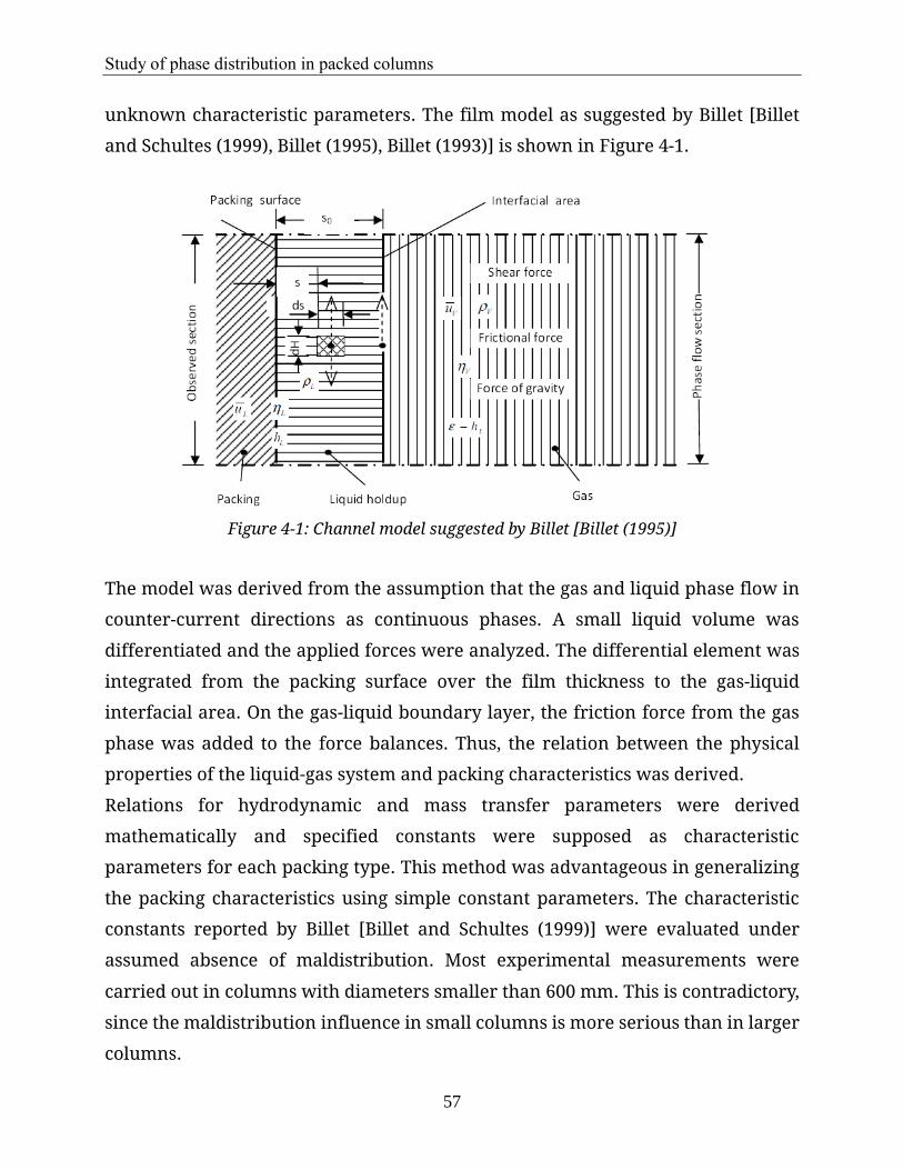
Study of phase distribution in packed columns
57
unknown characteristic parameters. The film model as suggested by Billet [Billet
and Schultes (1999), Billet (1995), Billet (1993)] is shown in Figure 4-1.
Figure 4-1: Channel model suggested by Billet [Billet (1995)]
The model was derived from the assumption that the gas and liquid phase flow in
counter-current directions as continuous phases. A small liquid volume was
differentiated and the applied forces were analyzed. The differential element was
integrated from the packing surface over the film thickness to the gas-liquid
interfacial area. On the gas-liquid boundary layer, the friction force from the gas
phase was added to the force balances. Thus, the relation between the physical
properties of the liquid-gas system and packing characteristics was derived.
Relations for hydrodynamic and mass transfer parameters were derived
mathematically and specified constants were supposed as characteristic
parameters for each packing type. This method was advantageous in generalizing
the packing characteristics using simple constant parameters. The characteristic
constants reported by Billet [Billet and Schultes (1999)] were evaluated under
assumed absence of maldistribution. Most experimental measurements were
carried out in columns with diameters smaller than 600 mm. This is contradictory,
since the maldistribution influence in small columns is more serious than in larger
columns.

Study of phase distribution in packed columns
58
The suspended droplet model (SDM) shown in Figure 4-2 suggested by Mackowiak
[Mackowiak (2010)] is based on experimental observations at high fractions of
liquid droplets within in the column. This mechanism of droplet formation was
experimental verified by studies carried out by Bornhütter [Bornhütter (1991)]. A
force balance analysis was established for a single droplet and droplet clusters
which were suspended inside the packed columns. It was thought that droplets
were formed before reaching the loading point and that the large amounts of liquid
droplets were the main reason for flooding effects. The model was applied for the
study of hydrodynamic parameters, e.g. pressure drop ΔP, liquid holdup hL, gas
load capacity FV. Mass transfer processes were not investigated using the
suspended droplet model.
Figure 4-2: Suspended droplet model (SDM) suggested by Mackowiak [Mackowiak
(2010)]
Stichlmair [Stichlmair et al. (1989)] applied the particle model for predicting the
pressure drop and the capacity of counter-current gas-liquid flow in random
packed columns. In this model, the random packing was conceived as a collection
of orbicular particles. The size of the orbicular particles was dependent on the beds
void fraction and the surface area of the packing. For increasing liquid flow rate,
the void fraction of the bed drops, the size of the particle increases and the pressure
drop increases as well. This model was used to predict the pressure drop in both
irrigated random and structured packings. This approach was derived on basis of
the dry pressure drop and was extended to irrigation applications by a correction
in the presence of liquid.

Study of phase distribution in packed columns
59
Experimental measurements of the pressure drop and the liquid holdup of
traditional random packings (e.g. Pallring) up to the loading point were predicted
more accurately with the model suggested by Billet. The reason for this is that the
traditional random packings have a relatively lower specific area and thus produce
a lower fraction of droplets. The main regime of the liquid flow is film flow.
Accordingly, above the loading point, the suspended droplet model describes the
pressure drop and liquid holdup more accurately, since liquid droplets are formed
in larger fraction.
4.1.1 Pressure drop
Based on the theoretical models, pressure drop of un-wetted and wetted packings
can be calculated. The pressure drop of packings is influenced by the ratio of the
specific surface area a of each packing to the packed volume of the column, the void
volume fraction ε, the gas load factor FV, the wall factor 𝐾 and friction coefficient ζ.
Billet [Billet and Schultes (1999)] suggested to use (eq. 4-1) for the prediction of the
dry pressure drop. The friction coefficient was calculated with the Reynolds
number 𝑅𝑒 and the packing specific pressure drop constant of an un-wetted
packing CP,0 by (eq. 4-2). A large number of CP,0 were determined experimentally.
The pressure drop of irrigated packings was calculated by (eq. 4-3). The gas flow
friction coefficient ζ was determined using the pressure drop constant of an
irrigated packing CP with (eq. 4-4). The irrigated pressure drop strongly depends
on the liquid holdup.
Similar to the model suggested by Billet, Stichlmair [Stichlmair et al. (1989)]
suggested to calculate the pressure drop using (eq. 4-5). The gas phase friction
coefficient was determined using Re of the gas phase and the constants C1, C2, C3 as
shown in (eq. 4-6).
The pressure drop equation suggested by Mackowiak [Mackowiak (2010)] is more
complicated than the methods introduced by Billet and Stichlmair. The pressure
drop of un-wetted packings was similarly computed, using (eq. 4-7). The resistance
coefficient ψ was calculated with the constants K1, K2, K3, K4, dependent on Re as
shown in (eq. 4-8) and (eq. 4-9).

Study of phase distribution in packed columns
60
The irrigated pressure drop was determined using (eq. 4-10). Here, the resistance
coefficient ψ was calculated using (eq. 4-11). μ in (eq. 4-11) is a packing type
dependent form factor and A as well as B were the experimentally fitted constants
for the determination the irrigated pressure drop.
The pressure drop is one of the most important parameters for packed columns.
The equations suggested by Billet [Billet and Schultes (1999)] were basically derived
on large amounts of experimental results measured at the Ruhr- University
Bochum. A large fraction of the experimental results used by Mackowiak
[Mackowiak (2010)] were also originated from Ruhr- University Bochum.
Table 4-1: Correlations for the prediction of pressure drop
Author Remarks Correlations
[Billet and Schultes (1999)]
pressure drop for unwetted packings
20 v vΔP u ρa 1
= ζH ε 2 K
20 v vΔP u ρa 1
= ζH ε 2 K
20 v vΔP u ρa 1
= ζH ε 2 K
(eq. 4-1)
pressure drop coefficient for unwetted packings 0 ,0 0.08
64 1.8( )P
V V
CRe Re
= + (eq. 4-2)
pressure drop for irrigated packings
2
3
1
2( )v V
L
uP a
H Kh
=
−
(eq. 4-3)
pressure drop coefficient for irrigated packings
1.5
0.08
1.5
64 1.8( )( )Re Re
13300exp( )
LP
v v
L
hC
Fra
−= +
(eq. 4-4)
[Stichlmair et al. (1989)]
pressure drop for irrigated packings ( )
2
3
4.652
4.65
1 10.125
1
1
/c
L
v v
hp
u ah
+
−
− − =
−
−
(eq. 4-5)
pressure drop constant of irrigated packings C1, C2 and C3 from experiments
1 230.5Re Rev v
C CC = + +
(eq. 4-6)
pressure drop for unwetted packings
20
0 3
3 1 1
4v v
P
P u
H d K
−=
(eq. 4-7)
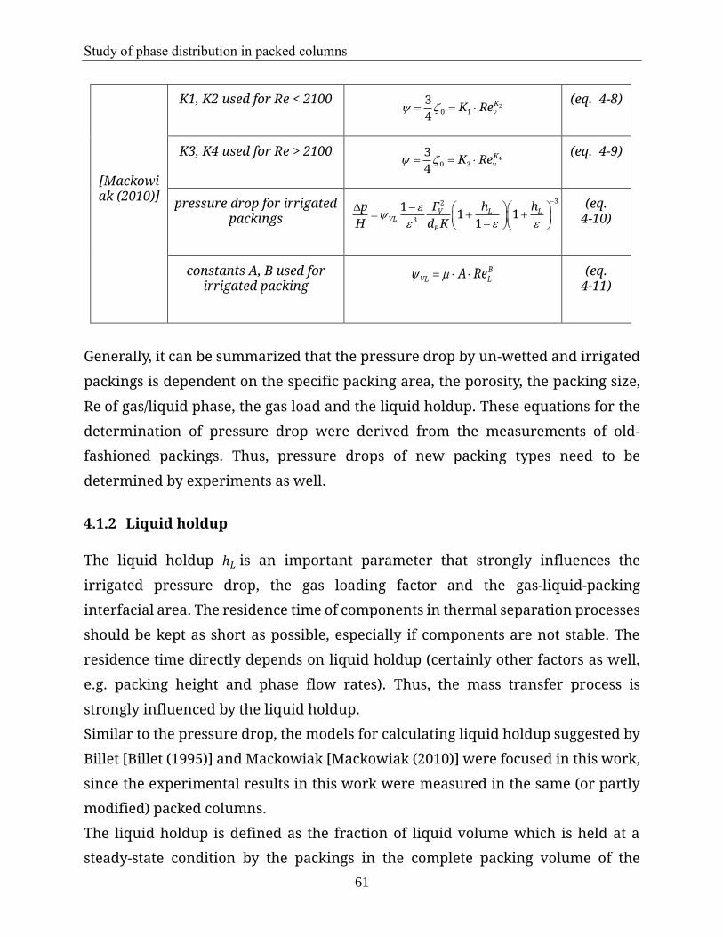
Study of phase distribution in packed columns
61
[Mackowiak (2010)]
K1, K2 used for Re < 2100 2
0 1
3
4KvK Re = =
(eq. 4-8)
K3, K4 used for Re > 2100 4
0 3
3
4KvK Re = =
(eq. 4-9)
pressure drop for irrigated packings
32
3
11 1
1V L L
VL
P
F h hp
H d K
− −
= + + −
(eq.
4-10)
constants A, B used for irrigated packing
BVL LA Re = (eq.
4-11)
Generally, it can be summarized that the pressure drop by un-wetted and irrigated
packings is dependent on the specific packing area, the porosity, the packing size,
Re of gas/liquid phase, the gas load and the liquid holdup. These equations for the
determination of pressure drop were derived from the measurements of old-
fashioned packings. Thus, pressure drops of new packing types need to be
determined by experiments as well.
4.1.2 Liquid holdup
The liquid holdup ℎ𝐿 is an important parameter that strongly influences the
irrigated pressure drop, the gas loading factor and the gas-liquid-packing
interfacial area. The residence time of components in thermal separation processes
should be kept as short as possible, especially if components are not stable. The
residence time directly depends on liquid holdup (certainly other factors as well,
e.g. packing height and phase flow rates). Thus, the mass transfer process is
strongly influenced by the liquid holdup.
Similar to the pressure drop, the models for calculating liquid holdup suggested by
Billet [Billet (1995)] and Mackowiak [Mackowiak (2010)] were focused in this work,
since the experimental results in this work were measured in the same (or partly
modified) packed columns.
The liquid holdup is defined as the fraction of liquid volume which is held at a
steady-state condition by the packings in the complete packing volume of the

Study of phase distribution in packed columns
62
packed column. In this sense, liquid holdup is a volume-averaged parameter.
Equations for the prediction of liquid holdup are listed in Table 4-2. The
dependency of liquid holdup on the gas load factor FV can be divided into three
areas:
1) Liquid holdup remains constant and is independent of the gas load Fv, if
superficial gas velocity is below the loading point Fv,S (Fv < Fv,S). The friction force
of the gas phase on the liquid phase at the phase interface is not large enough to
slow down the liquid phase. Increasing the gas load only leads to larger pressure
drop for any constant liquid irrigation rate. The liquid holdup is not influenced.
2) If the gas load exceeds the loading point, an increase of the liquid holdup can be
observed. With a further increase of the gas load, the local velocity of the liquid
inside the packing is slowed down by the gas phase. The liquid phase strongly
accumulates with further increase of the gas load. The tendency of the liquid
holdup increase is exponential.
3) The packed column floods, if the gas load factor reaches its maximum. At the
flooding point the pressure drop is so large that a further increase of the gas load
is not possible anymore.
As shown in Table 4-2, the calculation of the liquid holdup suggested by Billet is
influenced by the gas flow velocity uv, the gas density ρv, the pressure drop
coefficient ζ, the packing porosity ε, the packing specific area 𝑎, the liquid property
(e.g. liquid density ρL) and the liquid velocity uL. Liquid holdups below loading
point were determined using (eq. 4-17), in which the wetted area was determined
using equation (eq. 4-18) and (eq. 4-19). The liquid holdup above the loading point
was calculated using (eq. 4-20). Liquid holdup below the loading point is defined
as hL and liquid holdup above loading point as hL,S. One should be aware that the
exponent 13 in (eq. 4-20) indicates that the liquid holdup above the loading points
increases very quickly. However, it has been determined experimentally, that for
kinds of structured packings with high porosity, the exponent can be much smaller
(varies from 7 to 11). This exponent strongly depends on the packing form, packing
size and packing structure.
The average liquid thickness δL on the packing can be calculated with the liquid

Study of phase distribution in packed columns
63
holdup and the specific area a using (eq. 4-12).
δL=hL
a
(eq. 4-12)
The liquid film thickness δL shown in (eq. 4-13) was suggested by [Buchanan
(1969)] to determine the liquid holdup using (eq. 4-21).
δL= (3⋅η
l⋅uL
ρL
⋅g⋅a)
1/3
(eq. 4-13)
Mackowiak [Mackowiak (2010)] suggested to use (eq. 4-22) for calculation of the
liquid holdup. Liquid holdup in (eq. 4-22) is dependent on the gas load. If the
loading factor is larger than 65 % of gas load factor at the flooding point, (eq. 4-23)
should be used. The liquid holdup at the flooding point can theoretically be
determined using (eq. 4-24). The parameter 𝑚 depends on other quantities, e.g the
liquid phase Reynolds number ReL or the mass flow ratio of gas-liquid phase λ0. It
is determined using (eq. 4-25).
Stichlmair [Stichlmair et al. (1989)] studied the relations between the FrL and liquid
holdup based on experimental measurements. The relation was described by (eq.
4-26). FrL was defined by (eq. 4-14) as following.
FrL = uL2
a
gε4.65 (eq. 4-14)
FrL number used in (eq. 4-18) and (eq. 4-19) was calculated using (eq. 4-15).
FrL = uL
2 ⋅a
g
(eq. 4-15)
The liquid holdup above the loading point was calculated using (eq. 4-27), where
H is the total packing height and ΔP the pressure drop.
As shown in Table 4-2, liquid holdup strongly depends on the pressure drop,
packing size, packing materials, packing porosity and process condition and vice
versa. In these models the phase distribution was not considered and assumed as
uniform in the packings.

Study of phase distribution in packed columns
64
Table 4-2: Correlations for prediction of liquid holdup
Author Remarks Correlations
[Billet and Schultes (1999)]
2 1/ 2
2( )
3 4 ( )n L
L L L v v
L L
g aa u h u
h h
= −
−
(eq. 4-16)
Liquid holdup under the loading point ( )
,
1 22 3 3
, 12v v s
hL LL L su u
L
aa uh h
g a
= =
(eq. 4-17)
ReL < 5 0.25 0.10.85 Reh
h L L
aC Fr
a
=
(eq. 4-18)
ReL > 5 0.15 0.1Reh
h L L
aC Fr
a
=
(eq. 4-19)
Liquid holdup above the loading point ( )
13
, , ,
,
vL S L L FL L S
v Fl
uh h h h
u
= + −
(eq. 4-20)
[Buchanan (1969)]
( ) ( )1/3 1/32/33 /L L Lh g a u=
(eq. 4-21)
[Mackowiak (2010)]
Calculation of constant Pi ( )
( )11
mvLi L
L L
uuP h
h h + = −
−
(eq. 4-22)
𝑢𝑣 > 65% 𝑢𝑣,𝐹𝑙 1 1( (1 ) ( 1) )mv i L L Lu P h u h + −= − − −
(eq. 4-23)
phase flow ratio λ0 at flooding point
λ0=uL/uv
( ) ( ) ( ) ( )
( )( )L Fl
m m mh
m
+ + + − − +=
+ −
20 0 0 0
,
0
2 4 1 1 2
2 1 1
(eq. 4-24)
M = f(ReL, _0)
( )
1
,
,
0 ,
1 11
L Fl
L Fl
L Fl
hm h
h
−
= + −
−
(eq. 4-25)
[Stichlmair et al. (1989)]
e.g. C=0.555 for studied Raschig rings, Pallrings,
Hiflow, Mellapak, NSW rings,
Bialeckirings and Intalox
1/3L Lh C Fr=
(eq. 4-26)
2
, 1 20L S L
L
Ph h
H g
= +
(eq. 4-27)

Study of phase distribution in packed columns
65
4.1.3 Loading and flooding points
As discussed in chapter 4.1.2, gas loading capacity is limited by the gas load at the
loading and flooding point. Old-fashioned packings, e.g. Pallring and Raschig ring
have comparably lower loading and flooding points due to the fact that the porosity
of the packings is relatively low resulting in higher pressure drops. Although the
mass transfer rates of such packings are acceptable, high gas and liquid load
capacities are also important properties for achieving high time to volume
conversion.
The liquid holdup near the loading point is the most studied property of interest,
since industrial packed columns are usually operated close to the loading point.
Below the loading point, the pressure drop is small and the flow rate of gas is small
as well. Moreover, the mass transfer process is less efficient than the above loading
point, because above the loading point, the liquid flow is mainly turbulent. This
improves the mass transfer rates due to an enlarged interfacial area of the gas-
liquid phases. If the gas load factor is too high, the phase distribution is negatively
affected and strong maldistributions are formed. In this state, the mass transfer
rates are significantly reduced. The suggested gas load for optimized column
operation is 75% of the gas load at the flooding point as suggested by Mackowiak
[Mackowiak (2010)] is about 75 % of the gas capacity at the flooding point. The gas
loading capacity suggested Billet [Billet and Schultes (1999)] by was about 80 %.
This difference is dependent on the experimental packing types used for loading
point determination. For some of the new type packings, the loading point can be
larger than 85 % of the flooding load.
Generally, determination of loading and flooding points are performed at constant
liquid irrigation rates. As discussed in chapter 4.1.2, the liquid holdup begins to
increase at the loading point and reaches its maximum at the flooding point.
Calculations of the gas and liquid flow velocity at the loading point uv,S and uL,S and
flooding point uv,Fl and uL,Fl are shown in Table 4-3 .
The loading point constant CS in (eq. 4-28) was experimentally determined for
many kinds of packing. If CS is known, the friction coefficient ψS is evaluated using
(eq. 4-28). The gas flow velocity uv,Fl and liquid flow velocity uL,Fl at the loading

Study of phase distribution in packed columns
66
point are estimated using (eq. 4-29). Since the uv,Fl and uL,Fl are unknown variables,
(eq. 4-30) it is required to evaluate them iteratively.
Table 4-3: Determination of loading and flooding points using correlations as suggested by Billet [Billet and Schultes (1999)]
Author Remarks Correlations
[Billet and Schultes (1999)]
0.4, 0.723Vs
L
Ln
V
= −
0.4, 0.326Vs
L
Ln
V
= −
20.4
2
sn
v LS
L vS
g L
V etaC
−
=
(eq. 4-28)
, ,( )v S L Su f u= 1/3
1/2, ,1/6
1/6
,
112
112
Lv S L S
S L
L LL S
L v
gu a u
ga
ug
= −
(eq. 4-29)
, ,( )L S v Su f u= , ,
vL S v S
L
Lu u
V
=
(eq. 4-30)
0.4, 0.708Vs
L
Ln
V
= −
0.4, 0.194Vs
L
Ln
V
= −
20.2
2
Fln
v LFl
L vFl
g L
V etaC
−
=
(eq. 4-31)
, ,( )v Fl L Flu f h= ( )3 2, , ,
63 vL
L Fl L Fl v Fl
L L
Lh h a u
g V
− =
(eq. 4-32)
, ,( )v Fl v Flh f u= 1/4 1/2
1.2,
7/2
,1
h T LV F Fl
T V
L F
d d gu C
d
h
−
=
(eq. 4-33)
, ,( )L Fl v Flu f u= , ,
vL Fl v Fl
L
Lu u
V
=
(eq. 4-34)
Similar to the determination of the gas and liquid load at the loading point, the gas
and liquid flow rates at flooding point are evaluated iteratively as well. (eq. 4-31)

Study of phase distribution in packed columns
67
can be used for the evaluation of CFl, if CFl is known. The parameters for many kinds
of random and structured packings were reported by Billet [Billet and Schultes
(1999)]. Both, (eq. 4-32) and (eq. 4-33) contain two unknown variables, hv, Fl and
uv, Fl, which have to be evaluated iteratively as well. Thus, the liquid load can be
calculated using (eq. 4-34).
It is shown that determination of gas and liquid velocities at loading and flooding
point can be evaluated iteratively using the equations suggested by Billet [Billet and
Schultes (1999)]. The determination of loading and flooding points suggested by
Mackowiak [Mackowiak (2010)] are iteratively as well.
4.1.4 Mass transfer process
As previously explained, the pressure drop and liquid holdup is important for the
separation efficiency. The film model derived by Billet can also be applied for the
mass transfer process. Mass transfer parameters were suggested and reported in
Billet [Billet and Schultes (1999), Billet and Schultes (1995), Billet (1995), Billet and
Schultes (1993)]. The mass transfer process strongly depends on the
hydrodynamics of the absorption/ desorption process. In general, the mass transfer
process can be described using the equilibrium model and rate-based approaches.
4.1.4.1 Equilibrium model
The equilibrium stage model assumes that the gas and liquid phase leaving a tray
or a packing segment are in thermodynamical equilibrium with each other. The
equilibrium model for the description of separation processes was studied by
Henley [Henley and Seader (1981)]. As shown in Figure 4-3 (a), physical liquid
desorption (e.g., dilutet CO2 in H2O is stripped out of liquid phase by the gas phase)
mainly occurs at the top of the desorption column and physical gas absorption in
Figure 4-3 (b) (e.g., NH3 in air is absorbed though H2O phase) occurs in the bottom
range of the absorption column. The required packed height depends on the purity
requirements of the phases, gas and liquid flow rates and packing characteristics.
The equilibrium model assumes that the soluble component in the exiting gas and
liquid phase of each stage are in equilibrium. The equilibrium constant can be
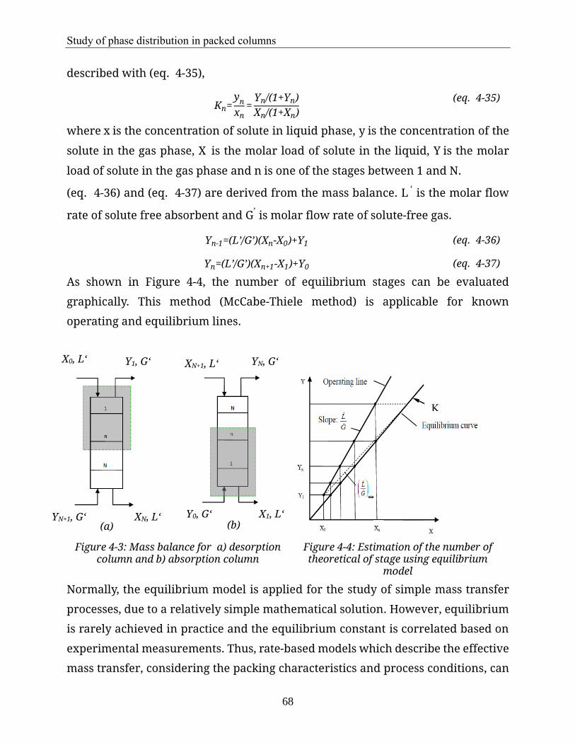
Study of phase distribution in packed columns
68
described with (eq. 4-35),
Kn=y
n
xn=
Yn/(1+Yn)
Xn/(1+Xn)
(eq. 4-35)
where x is the concentration of solute in liquid phase, y is the concentration of the
solute in the gas phase, X is the molar load of solute in the liquid, Y is the molar
load of solute in the gas phase and n is one of the stages between 1 and N.
(eq. 4-36) and (eq. 4-37) are derived from the mass balance. L ‘ is the molar flow
rate of solute free absorbent and G’ is molar flow rate of solute-free gas.
Yn-1=(L’/G’)(Xn-X0)+Y1 (eq. 4-36)
Yn=(L’/G’)(Xn+1-X1)+Y0 (eq. 4-37)
As shown in Figure 4-4, the number of equilibrium stages can be evaluated
graphically. This method (McCabe-Thiele method) is applicable for known
operating and equilibrium lines.
Figure 4-3: Mass balance for a) desorption column and b) absorption column
Figure 4-4: Estimation of the number of theoretical of stage using equilibrium
model
Normally, the equilibrium model is applied for the study of simple mass transfer
processes, due to a relatively simple mathematical solution. However, equilibrium
is rarely achieved in practice and the equilibrium constant is correlated based on
experimental measurements. Thus, rate-based models which describe the effective
mass transfer, considering the packing characteristics and process conditions, can
K
(a) (b) YN+1, G‘ XN, L‘
X0, L‘ Y1, G‘ YN, G‘ XN+1, L‘
Y0, G‘ X1, L‘
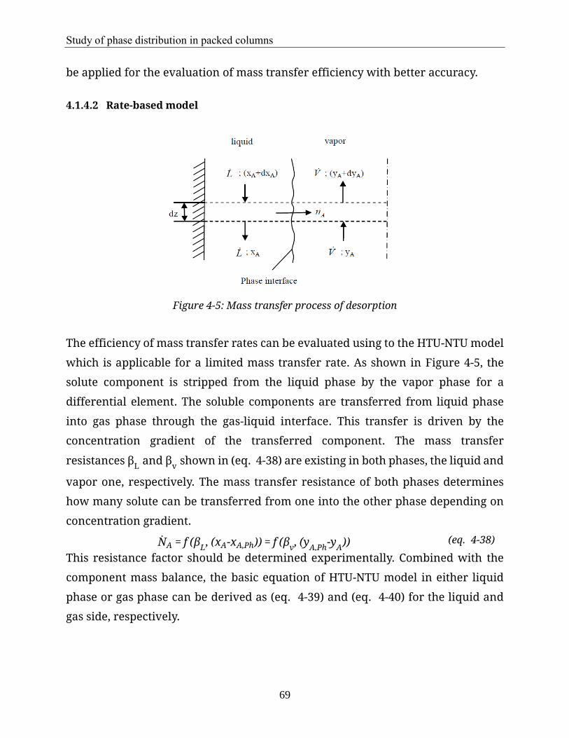
Study of phase distribution in packed columns
69
be applied for the evaluation of mass transfer efficiency with better accuracy.
4.1.4.2 Rate-based model
Figure 4-5: Mass transfer process of desorption
The efficiency of mass transfer rates can be evaluated using to the HTU-NTU model
which is applicable for a limited mass transfer rate. As shown in Figure 4-5, the
solute component is stripped from the liquid phase by the vapor phase for a
differential element. The soluble components are transferred from liquid phase
into gas phase through the gas-liquid interface. This transfer is driven by the
concentration gradient of the transferred component. The mass transfer
resistances βL and β
v shown in (eq. 4-38) are existing in both phases, the liquid and
vapor one, respectively. The mass transfer resistance of both phases determines
how many solute can be transferred from one into the other phase depending on
concentration gradient.
NA = f (βL, (xA-xA,Ph)) = f (β
v, (y
A,Ph-y
A)) (eq. 4-38)
This resistance factor should be determined experimentally. Combined with the
component mass balance, the basic equation of HTU-NTU model in either liquid
phase or gas phase can be derived as (eq. 4-39) and (eq. 4-40) for the liquid and
gas side, respectively.
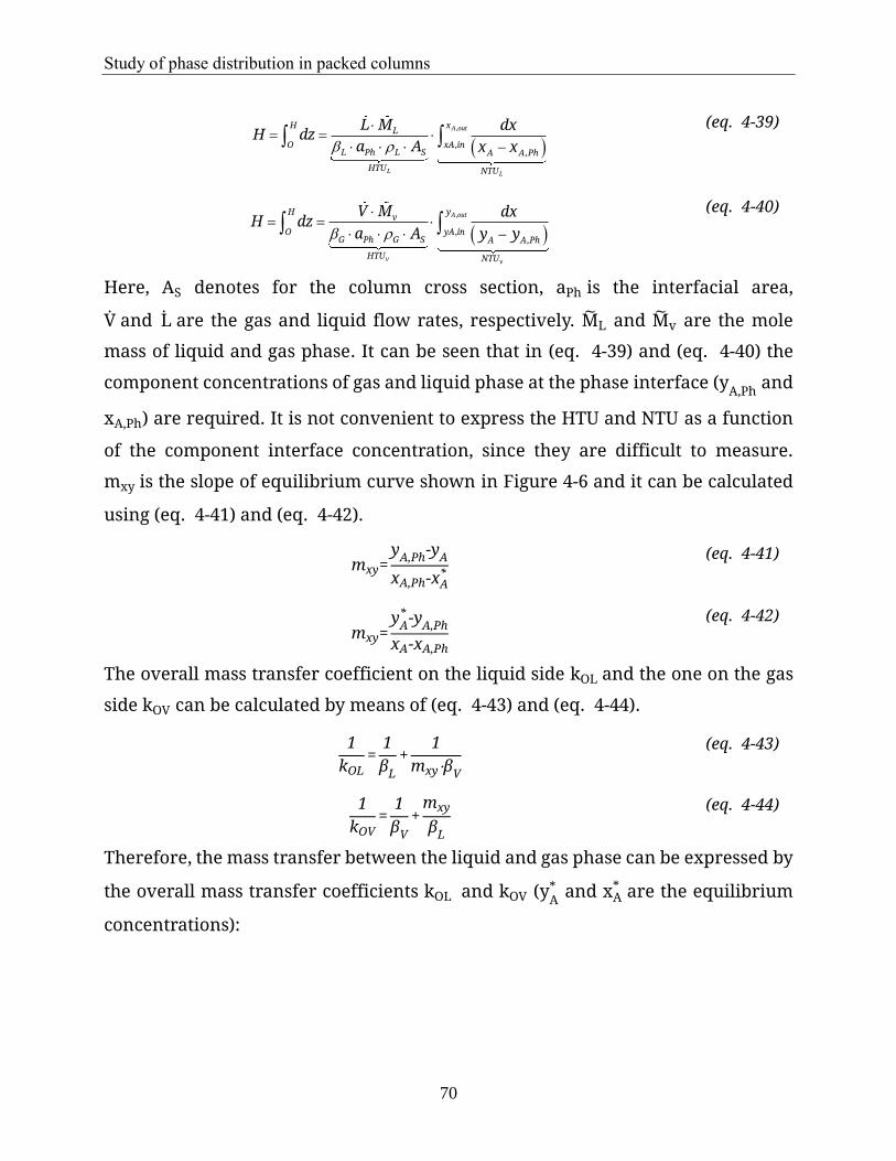
Study of phase distribution in packed columns
70
( )A,out
L L
H xL
O xA,inL Ph L S A A,Ph
HTU NTU
L M dxH dz
a A x x
= =
−
(eq. 4-39)
( ),
,,
A out
v v
H yv
O yA inG Ph G S A A Ph
HTU NTU
V M dxH dz
a A y y
= =
−
(eq. 4-40)
Here, AS denotes for the column cross section, aPh is the interfacial area,
V and L are the gas and liquid flow rates, respectively. ML and Mv are the mole
mass of liquid and gas phase. It can be seen that in (eq. 4-39) and (eq. 4-40) the
component concentrations of gas and liquid phase at the phase interface (yA,Ph
and
xA,Ph) are required. It is not convenient to express the HTU and NTU as a function
of the component interface concentration, since they are difficult to measure.
mxy is the slope of equilibrium curve shown in Figure 4-6 and it can be calculated
using (eq. 4-41) and (eq. 4-42).
mxy=y
A,Ph-y
A
xA,Ph-xA*
(eq. 4-41)
mxy=y
A* -y
A,Ph
xA-xA,Ph
(eq. 4-42)
The overall mass transfer coefficient on the liquid side kOL and the one on the gas
side kOV can be calculated by means of (eq. 4-43) and (eq. 4-44).
1
kOL=
1
βL
+1
mxy⋅βV
(eq. 4-43)
1
kOV=
1
βV
+mxy
βL
(eq. 4-44)
Therefore, the mass transfer between the liquid and gas phase can be expressed by
the overall mass transfer coefficients kOL and kOV (yA* and xA
* are the equilibrium
concentrations):
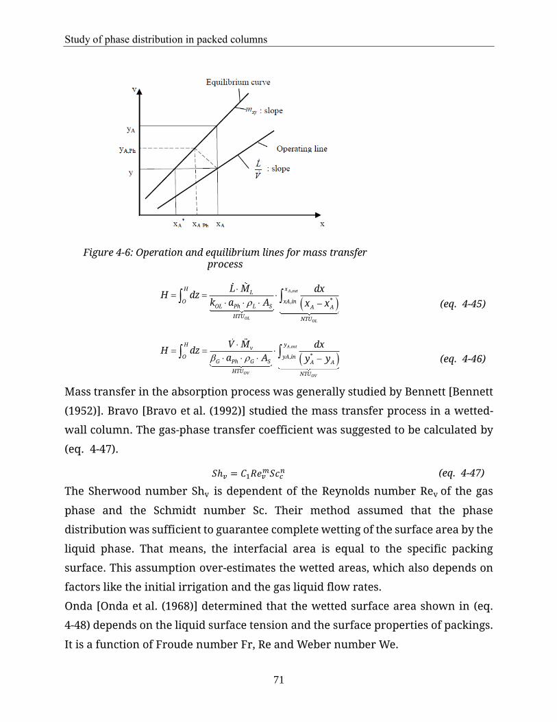
Study of phase distribution in packed columns
71
Figure 4-6: Operation and equilibrium lines for mass transfer process
( ),
*,
A out
OLOL
H xL
O xA inOL Ph L S A A
HTU NTU
L M dxH dz
k a A x x
= =
−
(eq. 4-45)
( ),
*,
A out
OVOV
H yv
O yA inG Ph G S A A
HTU NTU
V M dxH dz
a A y y
= =
−
(eq. 4-46)
Mass transfer in the absorption process was generally studied by Bennett [Bennett
(1952)]. Bravo [Bravo et al. (1992)] studied the mass transfer process in a wetted-
wall column. The gas-phase transfer coefficient was suggested to be calculated by
(eq. 4-47).
𝑆ℎ𝑣 = 𝐶1𝑅𝑒𝑣𝑚𝑆𝑐𝑐
𝑛 (eq. 4-47)
The Sherwood number Shv is dependent of the Reynolds number Rev of the gas
phase and the Schmidt number Sc. Their method assumed that the phase
distribution was sufficient to guarantee complete wetting of the surface area by the
liquid phase. That means, the interfacial area is equal to the specific packing
surface. This assumption over-estimates the wetted areas, which also depends on
factors like the initial irrigation and the gas liquid flow rates.
Onda [Onda et al. (1968)] determined that the wetted surface area shown in (eq.
4-48) depends on the liquid surface tension and the surface properties of packings.
It is a function of Froude number Fr, Re and Weber number We.

Study of phase distribution in packed columns
72
Aph
a=1-exp(-1.45(
σc
σL)0.75
ReL0.1FrL
-0.05WeL0.2)
(eq. 4-48)
Here, σc 𝑎𝑛𝑑 σL are the packing and liquid surface tensions, respectively.
Billet [Billet (1993)] suggested to calculate the wetted area using (eq. 4-49). The
dependency of the wetted area on Re, Fr and We are significantly different than
that in (eq. 4-48). This is the reason that the influence of surface tension is not
specified in (eq. 4-49) and organic solvent was especially applied to study the
influence of the liquid surface tension on the mass transfer process. Another reason
for the different approaches is that the measurements by Onda [Onda et al. (1968)]
mainly focused on the packing type Raschig rings.
Aph
a = 1.5(adh)
-0.5ReL
-0.2FrL-0.45WeL
0.75 (eq. 4-49)
Billet [Billet and Schultes (1999)] suggested to use (eq. 4-50) for the evaluation of
HTUOV (uV and uL are the gas and liquid superficial velocity).
HTUOV = uV
βV
⋅aPh+
mxy
L/V
uL
βL
⋅aPh
(eq. 4-50)
NTUOV, HTUOL and NTUOL were evaluated using (eq. 4-51) to (eq. 4-54).
H = HTUOV⋅NTUOV (eq. 4-51)
H=HTUOL⋅NTUOL (eq. 4-52)
HTUOL=HTUOV/λ (eq. 4-53)
NTUOL=λ⋅NTUOV (eq. 4-54)
The mass transfer coefficients of both phases can be evaluated with (eq. 4-55) and
(eq. 4-56). The constants CV and CL are the packing type specific constants for the
calculation of gas and liquid side limited mass transfer (HTU and NTU). The
influence of the liquid and gas phase flow rates on these parameters was also
studied. In these equations, HL’ is the holdup under the loading point, Dv is the
diffusion coefficient and dh is the equivalent diameter of one packing element.
βLaPh = CL⋅121/6
(uL
hL’
)
0.5
(D
dH)
0.5
a (aPh
a)
(eq. 4-55)

Study of phase distribution in packed columns
73
βV
aPh = CV⋅1
(ε-hL’
)0.5
a1.5
dh0.5
DV (uV
a∙νV)
0.75
(νV
DV)
1/3
(aPh
a)
(eq. 4-56)
The equations of mass transfer suggested and developed by Billet are considering
data of over 3500 experimental measurements, more than 50 different test systems
and were based on measurements with over 70 packing types. The model suggested
by Billet is widely accepted and applied. Within this work, the experimental
measurements, both the hydrodynamic and mass transfer measurements, were
mainly evaluated based on this model.
4.1.5 Study of phase distribution
The previously discussed models were derived from experimental observations
and are based on a uniform phase distribution. Non-uniform phase distribution,
which is defined as maldistribution as well, is related to column diameter, column
height, packing type and packing size, to name just a few. Maldistribution of the
liquid and gas phase can severely reduce packed column efficiency. Experimental
results should be analyzed, considering the maldistribution depending on the
column dimensions.
The study of liquid spreading using Gaussian distribution was suggested by Tour
[Tour and Lerman (1939)] to analyze their experimental results. It was concluded
that liquid spreading behaves similarly to the diffusion equation. Cihla [Cihla and
Schmidt (1957)] modified their study by introducing a partial differential equation
derived from the diffusion equation. They assumed that liquid spreading in the
horizontal direction is a random process and a function of the packing size.
Experimental and theoretical investigations of phase distribution in packed
columns are summarized in Table 4-4.
Cihla [Cihla and Schmidt (1957)] suggested to use a mathematical approach
(dispersion model) for the description of the trickling liquid phase in a random
packed column. In cylindrical packed columns different types of liquid distributors
were discussed. The packed height, column radius and liquid flow rates were
considered as influencing factors which play an important role in phase
distribution. The distribution of liquid flow over a layer of packing was interpreted
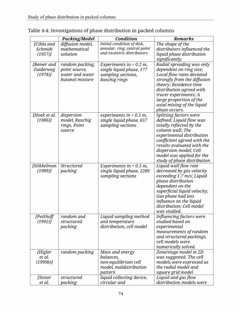
Study of phase distribution in packed columns
74
Table 4-4: Investigations of phase distribution in packed columns
Packing/Model Condition Remarks [Cihla and Schmidt (1957)]
diffusion model, mathematical solution
Initial condition of disk, annular, ring, central point and excentric distributors
The shape of the distributors influenced the liquid phase distribution significantly.
[Bemer and Zuiderweg
(1978)]
random packing, point source, water and water butanol mixture
Experiments in = 0.2 m, single liquid phase, 177 sampling sections, Raschig rings
Radial spreading was only dependent on ring size; Local flow rates deviated strongly from the diffusion theory; Residence time distribution agreed with tracer experiments; A large proportion of the axial mixing of the liquid phase occurs.
[Hoek et al. (1986)]
dispersion model, Raschig rings, Point source
experiments in = 0.5 m, single liquid phase, 657 sampling sections
Splitting factors were defined; Liquid flow was totally reflected by the column wall; The experimental distribution coefficient agreed with the results evaluated with the dispersion model; Cell model was applied for the study of phase distribution
[Stikkelman (1989)]
Structured packing
Experiments in = 0.5 m, single liquid phase, 1289 sampling sections
Liquid wall flow rate decreased by gas velocity exceeding 1.7 m/s; Liquid phase distribution dependent on the superficial liquid velocity; Gas phase had less influence on the liquid distribution; Cell model was studied.
[Potthoff (1992)]
random and structured packing
Liquid sampling method and temperature distribution, cell model
Influencing factors were studied based on experimental measurements of random and structured packings, cell models were numerically solved.
[Higler et al.
(1999b)]
random packing Mass and energy balances, non-equilibrium cell model, maldistribution pattern
Zone/stage model in 2D was suggested. The cell models were expressed as the radial model and square grid model
[Stoter et al.
structured packing
liquid collecting device, circular and
Liquid and gas flow distribution models were
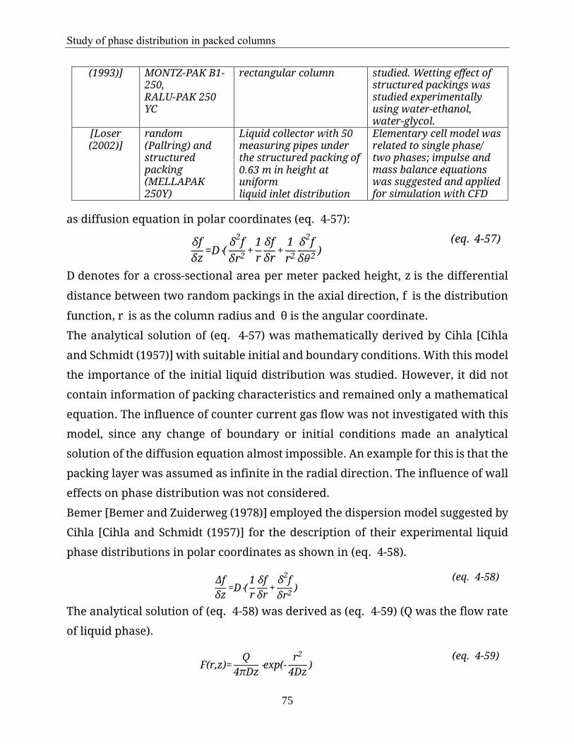
Study of phase distribution in packed columns
75
(1993)] MONTZ-PAK B1-250, RALU-PAK 250 YC
rectangular column studied. Wetting effect of structured packings was studied experimentally using water-ethanol, water-glycol.
[Loser (2002)]
random (Pallring) and structured packing (MELLAPAK 250Y)
Liquid collector with 50 measuring pipes under the structured packing of 0.63 m in height at uniform liquid inlet distribution
Elementary cell model was related to single phase/ two phases; impulse and mass balance equations was suggested and applied for simulation with CFD
as diffusion equation in polar coordinates (eq. 4-57):
δf
δz=D⋅(
δ2f
δr2+
1
r
δf
δr+
1
r2
δ2f
δ𝜃2)
(eq. 4-57)
D denotes for a cross-sectional area per meter packed height, z is the differential
distance between two random packings in the axial direction, f is the distribution
function, r is as the column radius and θ is the angular coordinate.
The analytical solution of (eq. 4-57) was mathematically derived by Cihla [Cihla
and Schmidt (1957)] with suitable initial and boundary conditions. With this model
the importance of the initial liquid distribution was studied. However, it did not
contain information of packing characteristics and remained only a mathematical
equation. The influence of counter current gas flow was not investigated with this
model, since any change of boundary or initial conditions made an analytical
solution of the diffusion equation almost impossible. An example for this is that the
packing layer was assumed as infinite in the radial direction. The influence of wall
effects on phase distribution was not considered.
Bemer [Bemer and Zuiderweg (1978)] employed the dispersion model suggested by
Cihla [Cihla and Schmidt (1957)] for the description of their experimental liquid
phase distributions in polar coordinates as shown in (eq. 4-58).
Δf
δz=D⋅(
1
r
δf
δr+
δ2f
δr2)
(eq. 4-58)
The analytical solution of (eq. 4-58) was derived as (eq. 4-59) (Q was the flow rate
of liquid phase).
F(r,z)=Q
4πDz⋅exp(-
r2
4Dz)
(eq. 4-59)

Study of phase distribution in packed columns
76
In the experimental measurements shown in Figure 4-7, performed by Bemer
[Bemer and Zuiderweg (1978)], the liquid collector was divided into 177 sampling
cells (with each cell size having 16x16 mm2).
Due to the small scale of the cells, local distribution was investigated on the scale
of a single packing element. Underneath the support plate a collection device was
installed. As irrigating liquids, both tap water and mixtures of water/ butanol were
used while the column was filled with glass and Teflon coated Raschig Rings of
different size (dP = 0.01 - 0.03 m). Superficial liquid velocity uL was varied between
2 and 30 m3/m2/h at packed heights between 5 and 30 cm. It was found that wetting
properties had no noticeable influence on the flow distribution, since typical
channeling of liquid in random packing was observed independently of the packing
wettability.
As shown in Figure 4-8, Hoek [Hoek et al. (1986)] used similar equipment as [Bemer
and Zuiderweg (1978)]. The packing height was varied up to two meters and a
distributor with 68 nozzles of 3.0 mm diameter (approximately 350 nozzles/m2,
irrigation diameter < 0.45 m) was used. It was suggested to analyze the flow
patterns measured after several splittings of the liquid flow and thus after several
packing layers, where the flow patterns were smooth and of regular shape. At the
given packed height, 12 packing layers were installed. The diffusion equation (eq.
4-58) was applied to study the flow patterns. From these flow patterns the
distribution coefficient Dr was determined as 0.0029 m for 25 mm Raschig Rings. It
was reported that the value was similar to the one in their experimental study.

Study of phase distribution in packed columns
77
Figure 4-7: Experimental setup used by Bemer [Bemer and Zuiderweg
(1978)]
Figure 4-8: Experimental setup used by Hoek [Hoek et al. (1986)]
For the flow pattern shown in Figure 4-9, a regular liquid flow distribution without
channeling was observed. It was found that Dr was 0.03 m for the structured
packing Mellapak at a certain packing height and liquid flow rate. Based on their
experimental results, large scale maldistribution was also studied and a correlation
for the description of liquid wall flow was suggested.
Figure 4-9: Liquid phase distribution studied by Hoek [Hoek et al. (1986)]
The effects of gas load on the liquid distribution were studied experimentally by

Study of phase distribution in packed columns
78
Stikkelman [Stikkelman (1989)]. His experimental results showed that the liquid
bulk flow became less uniform as the superficial liquid velocity was diminished.
However, the flow distribution was almost independent of the gas flow. The
spreading pattern of liquid flow showed a small increase up to the loading point
and a more rapid increase above it. Radial spreading mechanisms shown in Figure
4-10 were applied for the description of the phase distributions using a cell model.
The liquid flow downwards from an overlying cell is splitted: One part of the liquid
flows downward vertically, to the underlying central cell. The rest of the liquid is
symmetrically divided into the four adjacent cells of the underlying central cell.
The gas phase, which flows counter current, was described with a similar splitting
mechanism, whereby the splitting factor differed from the one of the liquid phase.
The splitting factors were experimentally determined by point source experiments.
Compared to the cell model suggested by Potthoff [Potthoff (1992)], Stikkelman
[Stikkelman (1989)] considered less cells within the splitting process. By the model
suggested Potthoff [Potthoff (1992)], it was assumed that at each cell plane both, the
gas and liquid phases are flowing in slug flow. The separation efficiency NTUOV
was evaluated using the mass transfer coefficients discussed in the previous
chapter. The cells at the column wall were considered as well. The gas and liquid
flows in the cells at the column wall were assumed as ideal counter current.
Figure 4-10: Cell model as suggested by Stikkelman [Stikkelman (1989)]
Figure 4-11: Cell model as suggested by Potthoff [Potthoff (1992)]
Billingham [Billingham et al. (1997)] suggested to define the radial spreading
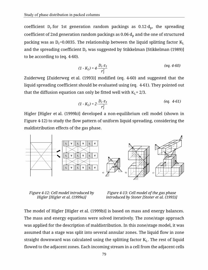
Study of phase distribution in packed columns
79
coefficient Dr for 1st generation random packings as 0.12∙dp, the spreading
coefficient of 2nd generation random packings as 0.06∙dp and the one of structured
packing was as Dr=0.0035. The relationship between the liquid splitting factor KL
and the spreading coefficient Dr was suggested by Stikkelman [Stikkelman (1989)]
to be according to (eq. 4-60).
(1 - KL) = 4⋅Dr⋅z1
r12
(eq. 4-60)
Zuiderweg [Zuiderweg et al. (1993)] modified (eq. 4-60) and suggested that the
liquid spreading coefficient should be evaluated using (eq. 4-61). They pointed out
that the diffusion equation can only be fitted well with KL= 2/3.
(1 - KL) = 2⋅Dr⋅z1
r12
(eq. 4-61)
Higler [Higler et al. (1999b)] developed a non-equilibrium cell model (shown in
Figure 4-12) to study the flow pattern of uniform liquid spreading, considering the
maldistribution effects of the gas phase.
Figure 4-12: Cell model introduced by Higler [Higler et al. (1999a)]
Figure 4-13: Cell model of the gas phase introduced by Stoter [Stoter et al. (1993)]
The model of Higler [Higler et al. (1999b)] is based on mass and energy balances.
The mass and energy equations were solved iteratively. The zone/stage approach
was applied for the description of maldistribution. In this zone/stage model, it was
assumed that a stage was split into several annular zones. The liquid flow in zone
straight downward was calculated using the splitting factor KL. The rest of liquid
flowed to the adjacent zones. Each incoming stream in a cell from the adjacent cells
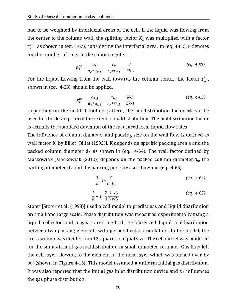
Study of phase distribution in packed columns
80
had to be weighted by interfacial areas of the cell. If the liquid was flowing from
the center to the column wall, the splitting factor KL was multiplied with a factor
rkao , as shown in (eq. 4-62), considering the interfacial area. In (eq. 4-62), k denotes
for the number of rings to the column center.
Rkao =
ak
ak+ak-1 =
rk
rk+rk-1 =
k
2k-1
(eq. 4-62)
For the liquid flowing from the wall towards the column center, the factor rkai ,
shown in (eq. 4-63), should be applied.
Rkao =
ak-1
ak+ak-1 =
rk-1
rk+rk-1 =
k-1
2k-1
(eq. 4-63)
Depending on the maldistribution pattern, the maldistribution factor Mf can be
used for the description of the extent of maldistribution. The maldistribution factor
is actually the standard deviation of the measured local liquid flow rates.
The influence of column diameter and packing size on the wall flow is defined as
wall factor K by Billet [Billet (1995)]. K depends on specific packing area a and the
packed column diameter dS as shown in (eq. 4-64). The wall factor defined by
Mackowiak [Mackowiak (2010)] depends on the packed column diameter ds, the
packing diameter dP and the packing porosity ϵ as shown in (eq. 4-65).
1
k=1+
4
a∙ds
(eq. 4-64)
1
k = 1+
2
3
1
1-ϵ
dP
dS
(eq. 4-65)
Stoter [Stoter et al. (1993)] used a cell model to predict gas and liquid distribution
on small and large scale. Phase distribution was measured experimentally using a
liquid collector and a gas tracer method. He observed liquid maldistribution
between two packing elements with perpendicular orientation. In the model, the
cross section was divided into 12 squares of equal size. The cell model was modified
for the simulation of gas maldistribution in small diameter columns. Gas flow left
the cell layer, flowing to the element in the next layer which was turned over by
90∘ (shown in Figure 4-13). This model assumed a uniform initial gas distribution.
It was also reported that the initial gas inlet distribution device and 𝑅𝑒 influences
the gas phase distribution.
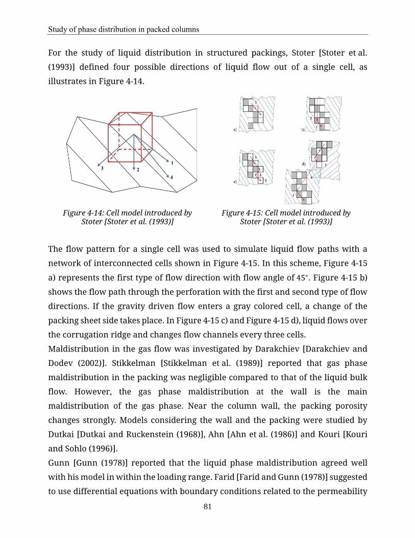
Study of phase distribution in packed columns
81
For the study of liquid distribution in structured packings, Stoter [Stoter et al.
(1993)] defined four possible directions of liquid flow out of a single cell, as
illustrates in Figure 4-14.
Figure 4-14: Cell model introduced by Stoter [Stoter et al. (1993)]
Figure 4-15: Cell model introduced by Stoter [Stoter et al. (1993)]
The flow pattern for a single cell was used to simulate liquid flow paths with a
network of interconnected cells shown in Figure 4-15. In this scheme, Figure 4-15
a) represents the first type of flow direction with flow angle of 45∘. Figure 4-15 b)
shows the flow path through the perforation with the first and second type of flow
directions. If the gravity driven flow enters a gray colored cell, a change of the
packing sheet side takes place. In Figure 4-15 c) and Figure 4-15 d), liquid flows over
the corrugation ridge and changes flow channels every three cells.
Maldistribution in the gas flow was investigated by Darakchiev [Darakchiev and
Dodev (2002)]. Stikkelman [Stikkelman et al. (1989)] reported that gas phase
maldistribution in the packing was negligible compared to that of the liquid bulk
flow. However, the gas phase maldistribution at the wall is the main
maldistribution of the gas phase. Near the column wall, the packing porosity
changes strongly. Models considering the wall and the packing were studied by
Dutkai [Dutkai and Ruckenstein (1968)], Ahn [Ahn et al. (1986)] and Kouri [Kouri
and Sohlo (1996)].
Gunn [Gunn (1978)] reported that the liquid phase maldistribution agreed well
with his model in within the loading range. Farid [Farid and Gunn (1978)] suggested
to use differential equations with boundary conditions related to the permeability
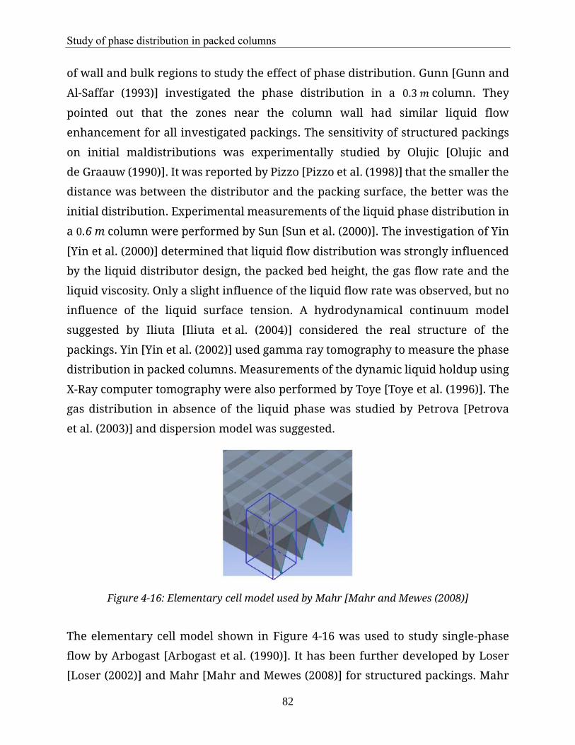
Study of phase distribution in packed columns
82
of wall and bulk regions to study the effect of phase distribution. Gunn [Gunn and
Al-Saffar (1993)] investigated the phase distribution in a 0.3 𝑚 column. They
pointed out that the zones near the column wall had similar liquid flow
enhancement for all investigated packings. The sensitivity of structured packings
on initial maldistributions was experimentally studied by Olujic [Olujic and
de Graauw (1990)]. It was reported by Pizzo [Pizzo et al. (1998)] that the smaller the
distance was between the distributor and the packing surface, the better was the
initial distribution. Experimental measurements of the liquid phase distribution in
a 0.6 m column were performed by Sun [Sun et al. (2000)]. The investigation of Yin
[Yin et al. (2000)] determined that liquid flow distribution was strongly influenced
by the liquid distributor design, the packed bed height, the gas flow rate and the
liquid viscosity. Only a slight influence of the liquid flow rate was observed, but no
influence of the liquid surface tension. A hydrodynamical continuum model
suggested by Iliuta [Iliuta et al. (2004)] considered the real structure of the
packings. Yin [Yin et al. (2002)] used gamma ray tomography to measure the phase
distribution in packed columns. Measurements of the dynamic liquid holdup using
X-Ray computer tomography were also performed by Toye [Toye et al. (1996)]. The
gas distribution in absence of the liquid phase was studied by Petrova [Petrova
et al. (2003)] and dispersion model was suggested.
Figure 4-16: Elementary cell model used by Mahr [Mahr and Mewes (2008)]
The elementary cell model shown in Figure 4-16 was used to study single-phase
flow by Arbogast [Arbogast et al. (1990)]. It has been further developed by Loser
[Loser (2002)] and Mahr [Mahr and Mewes (2008)] for structured packings. Mahr

Study of phase distribution in packed columns
83
[Mahr and Mewes (2008)] studied phase distribution in MELLAPAK 250.Y (PP)
experimentally using x-Ray tomography and described the phase distribution with
the elementary cell model. The cell model shown in Figure 4-16 suggested by Loser
[Loser (2002)] and Mahr [Mahr and Mewes (2008)] is focused on the smallest
periodic elementary cell, which was used to describe the phase flow within the
whole packing. The smallest representative cell can be chosen as one or two cells.
The conservation equations of mass and momentum were applied for each
elementary cell. Due to its channel structure, corrugated structured packings
strongly feature the preference of certain flow directions. The anisotropic flow
resistance for the gas phase was modeled using a direction dependent resistance
coefficient. The liquid phase was split up into two sub-phases to separately model
the flow along each preferential flow direction. The force balance of the gas and
liquid phases were based on the liquid film flow on an inclined plate with counter-
current gas flow, that was suggested by Brauer [Brauer (1971)].
4.2 Experimental study of packed column
Pressure drop, liquid holdup and mass transfer in packed a column, which was
filled with random or structured packings, were experimentally studied at
different gas loads and without counter current gas flow. Experimental
measurements were carried out in packed column with diameter of 288 mm. A
liquid collector was applied for the measurements of the liquid fraction at the
column wall. A capacitive WMS was applied for the phase distribution
measurements in the packed column.
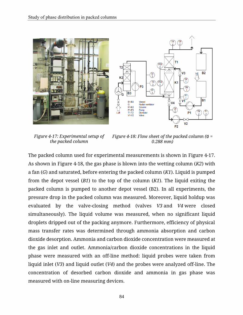
Study of phase distribution in packed columns
84
Figure 4-17: Experimental setup of
the packed column Figure 4-18: Flow sheet of the packed column (∅ =
0.288 mm)
The packed column used for experimental measurements is shown in Figure 4-17.
As shown in Figure 4-18, the gas phase is blown into the wetting column (K2) with
a fan (G) and saturated, before entering the packed column (K1). Liquid is pumped
from the depot vessel (B1) to the top of the column (K1). The liquid exiting the
packed column is pumped to another depot vessel (B2). In all experiments, the
pressure drop in the packed column was measured. Moreover, liquid holdup was
evaluated by the valve-closing method (valves V3 and V4 were closed
simultaneously). The liquid volume was measured, when no significant liquid
droplets dripped out of the packing anymore. Furthermore, efficiency of physical
mass transfer rates was determined through ammonia absorption and carbon
dioxide desorption. Ammonia and carbon dioxide concentration were measured at
the gas inlet and outlet. Ammonia/carbon dioxide concentrations in the liquid
phase were measured with an off-line method: liquid probes were taken from
liquid inlet (V3) and liquid outlet (V4) and the probes were analyzed off-line. The
concentration of desorbed carbon dioxide and ammonia in gas phase was
measured with on-line measuring devices.

Study of phase distribution in packed columns
85
4.2.1.1 Study of hydrodynamics in structured packing
The operating conditions for the hydrodynamic measurements of structured
packings (type A and type B) are shown in Table 4-5. Both structured packings had
the same specific area, porosity and structure. The packing types differed only in
the packing surfaces. The studied packed heights for both structured packings were
1.86 m and 1.54 m, respectively. The gas load factors Fv were varied from
0.5 Pa0.5 to 4.0 Pa0.5 , while the liquid loads 0, 10, 20, 30 to 40 m3/m2/h were
investigated.
Table 4-5: Structured packing used in packed column
Structured packing type A Structured packing type B
specific area a 240 m2/m3 240 m2/m3
porosity ε 0.945 0.945
packed height H 1.86 m 1.54 m
gas load factor FV 0.5 Pa0.5 - 4.0 Pa0.5 0.5 Pa0.5 - 4.0 Pa0.5
liquid load factor u𝐿 0, 10, 20, 30, 40 m3/m2/h 0, 10, 20, 30, 40 m3/m2/h
It is seen from Figure 4-19 that the specific pressure drops of both structured
packings are very similar. The constant parameter CP which was calculated using
(eq. 4-1) to (eq. 4-4) is shown in Table 4-6. It indicates that the roughness of the
packing surfaces does not significantly influences the pressure drop.
Typ A
Typ B
Figure 4-19: Pressure drop of different types of structured packing

Study of phase distribution in packed columns
86
The liquid holdup of type A and type B is shown in Figure 4-20. Unlike the pressure
drop, the liquid holdup of both structured packings significantly differs from each
other at different liquid flow rates. The liquid holdup plot of type 𝐴 is relatively
typical, as the loading and flooding condition are clearly recognized. The liquid
holdup of type 𝐵 is non-typical, since the loading and flooding points are difficult
to recognize.
Type A Type B
Figure 4-20: Liquid holdup of of different types of structured packing
Moreover, the loading point at a liquid flow rate of 10 m3/m2/h is smaller for type
B than for type A. The difference was most likely caused by the roughness of the
packing surfaces or the different packed heights resulting in in different phase
distributions (packing heights of type A and type B are 1.86 m and 1.54 m,
respectively). The holdup constant Ch was determined using (eq. 4-16) to (eq. 4-20)
for both structured packings.
The constants calculated for the Billet method for type A and type B are
summarized in Table 4-6 and Table 4-7, respectively.
It can be recognized that the constants CP and Ch of structured packings type 𝐴 and
type 𝐵 are relatively independent on the liquid flow rates, slightly on the gas load
factors below the loading point and strongly on the gas load above the loading
point. The constants CP and Ch of both packing types A and B differ significantly
from each other, since the surface roughness of both structured packings is
different.

Study of phase distribution in packed columns
87
Table 4-6: Characteristic constants of structured packing type A
Table 4-7: Characteristic constants of structured packing type B
𝑢𝐿 [m³/m²/h]
𝐹𝑉 [𝑃𝑎0.5]
𝐶𝑃 [-]
𝐶ℎ [-]
𝐶𝑆 [-]
𝐶𝐹𝑙 [-]
𝑢𝐿 [m³/m²/h]
𝐹𝑉 [𝑃𝑎0.5]
𝐶𝑃 [-]
𝐶ℎ [-]
𝐶𝑆 [-]
𝐶𝐹𝑙 [-]
0 0.885 0.144 - - - 0 0.877 0.148 - - - 0 1.630 0.154 - - - 0 1.630 0.159 - - - 0 2.185 0.157 - - - 0 2.184 0.158 - - - 0 2.674 0.157 - - - 0 2.674 0.161 - - - 0 3.039 0.157 - - - 0 3.052 0.162 - - - 0 3.443 0.158 - - - 0 3.454 0.160 - - - 0 3.763 0.156 - - - 0 3.800 0.160 - - -
10 0.880 0.204 0.320
3.170
2.452
10 0.877 0.222 0.351
3.194
2.474
10 1.740 0.227 0.320 10 1.590 0.229 0.336 10 2.298 0.226 0.339 10 2.261 0.223 0.425 10 2.637 0.227 0.359 10 2.601 0.223 0.517 10 2.895 0.241 0.339 10 2.894 0.216 0.586 10 3.345 0.252 0.400 10 3.341 0.226 0.704 10 3.472 0.269 0.442 10 3.511 0.243 0.828 20 0.890 0.197 0.286
3.548
2.756
20 0.934 0.196 0.428
3.713
2.910
20 1.740 0.217 0.263 20 1.694 0.199 0.506 20 2.323 0.214 0.323 20 2.286 0.198 0.545 20 2.567 0.227 0.310 20 2.578 0.202 0.556 20 2.868 0.244 0.335 20 2.879 0.208 0.567 20 3.149 0.274 0.374 20 3.157 0.242 0.622 20 3.397 0.291 0.497 20 3.635 0.308 0.659 30 0.885 0.183 0.255
3.908
3.053
30 0.826 0.196 0.362
3.940
3.083
30 1.639 0.218 0.246 30 1.599 0.205 0.386 30 2.145 0.219 0.255 30 2.099 0.201 0.481 30 2.395 0.219 0.282 30 2.323 0.200 0.462 30 2.728 0.230 0.368 30 2.743 0.212 0.574 30 2.962 0.252 0.506 30 2.914 0.243 0.591 30 3.500 0.336 0.745 30 3.543 0.331 0.833 40 0.903 0.189 0.295
3.933
3.044
40 0.852 0.184 0.387
4.055
3.157
40 1.673 0.203 0.279 40 1.608 0.193 0.450 40 2.311 0.206 0.350 40 2.191 0.190 0.521 40 2.578 0.217 0.427 40 2.561 0.190 0.590 40 2.739 0.255 0.508 40 2.743 0.224 0.643 40 3.053 0.317 0.634 40 3.052 0.316 0.802 40 3.251 0.344 0.715 40 3.402 0.405 0.854
The constants of loading (CS) and flooding (CFl) capacity factors, which are shown
in Table 4-6 and Table 4-7, were evaluated using (eq. 4-28) to (eq. 4-34). It can be
seen that the constants CS and CFl are dependent on the liquid flow rates. They are
almost constant at larger liquid flow rates (at 𝑢𝐿= 30 m3/m2/h and 𝑢𝐿= 40 m3/m2/h)
for both packing types. It should be noted that the description of pressure drop,
liquid holdup, loading and flooding points using only one constant CP, Ch, CS and
CFl can lead to relative large deviation, since the constants depend on liquid phase
flow rates or gas loading factors.
4.2.1.2 Study of hydrodynamics in random packing
Pallrings (∅ = 25 mm, a = 225 m2/m3, ϵ = 0.95) were applied with a packed height of

Study of phase distribution in packed columns
88
2 m. In Figure 4-21, the pressure drop at different liquid flow rates (∅ = 288 mm) is
illustrated. The comparison of the pressure drops of Palling’s, structured packing’s
type A and type B shows that the pressure drop of the Pallrings is significantly larger
at all studied liquid flow rates, although the specific area is slightly lower.
Figure 4-21: Pressure drop of Pallrings (25 𝑚𝑚, metal) in a packed column (𝜙=288 𝑚𝑚)
The liquid holdup of the Pallrings is shown in Figure 4-22. It was observed that the
liquid holdup can be well described by the discussed equations (see Billet method).
Figure 4-22: Liquid holdup of Pallring (25 𝑚𝑚) Metall in packed column (𝜙 =288 𝑚𝑚)
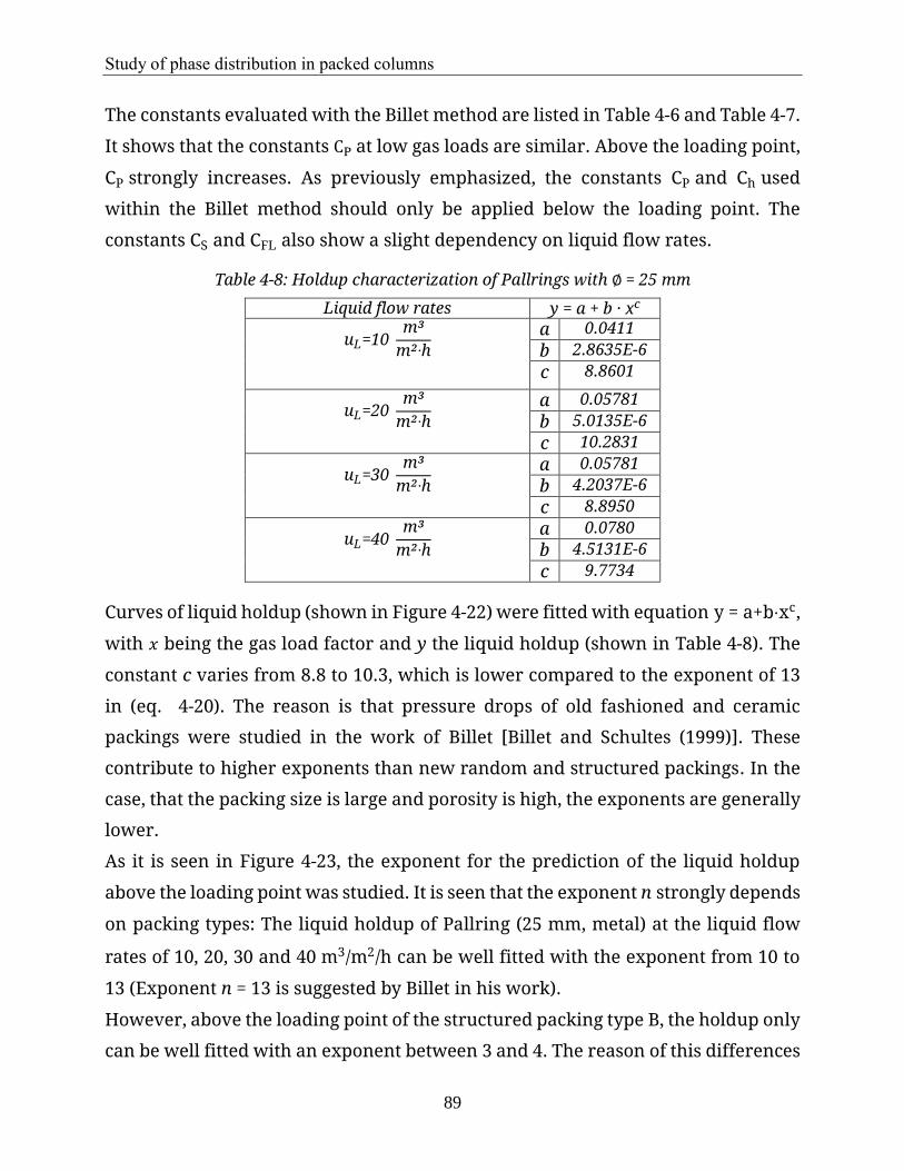
Study of phase distribution in packed columns
89
The constants evaluated with the Billet method are listed in Table 4-6 and Table 4-7.
It shows that the constants CP at low gas loads are similar. Above the loading point,
CP strongly increases. As previously emphasized, the constants CP and Ch used
within the Billet method should only be applied below the loading point. The
constants CS and CFL also show a slight dependency on liquid flow rates.
Table 4-8: Holdup characterization of Pallrings with ∅ = 25 mm
Liquid flow rates y = a + b · xc
uL=10 m³
m²∙h
a 0.0411
b 2.8635E-6
c 8.8601
uL=20 m³
m²∙h
a 0.05781
b 5.0135E-6
c 10.2831
uL=30 m³
m²∙h
a 0.05781
b 4.2037E-6
c 8.8950
uL=40 m³
m²∙h
a 0.0780
b 4.5131E-6
c 9.7734
Curves of liquid holdup (shown in Figure 4-22) were fitted with equation y = a+b⋅xc,
with 𝑥 being the gas load factor and y the liquid holdup (shown in Table 4-8). The
constant c varies from 8.8 to 10.3, which is lower compared to the exponent of 13
in (eq. 4-20). The reason is that pressure drops of old fashioned and ceramic
packings were studied in the work of Billet [Billet and Schultes (1999)]. These
contribute to higher exponents than new random and structured packings. In the
case, that the packing size is large and porosity is high, the exponents are generally
lower.
As it is seen in Figure 4-23, the exponent for the prediction of the liquid holdup
above the loading point was studied. It is seen that the exponent n strongly depends
on packing types: The liquid holdup of Pallring (25 mm, metal) at the liquid flow
rates of 10, 20, 30 and 40 m3/m2/h can be well fitted with the exponent from 10 to
13 (Exponent n = 13 is suggested by Billet in his work).
However, above the loading point of the structured packing type B, the holdup only
can be well fitted with an exponent between 3 and 4. The reason of this differences
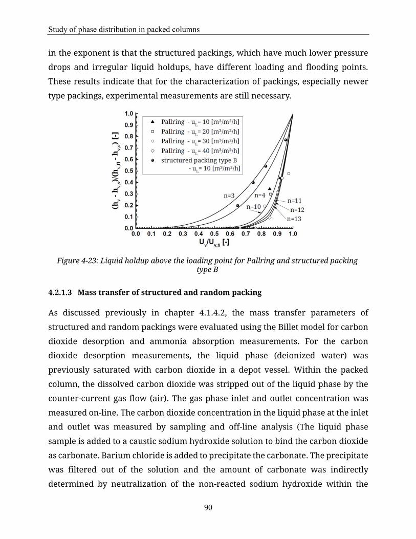
Study of phase distribution in packed columns
90
in the exponent is that the structured packings, which have much lower pressure
drops and irregular liquid holdups, have different loading and flooding points.
These results indicate that for the characterization of packings, especially newer
type packings, experimental measurements are still necessary.
Figure 4-23: Liquid holdup above the loading point for Pallring and structured packing type B
4.2.1.3 Mass transfer of structured and random packing
As discussed previously in chapter 4.1.4.2, the mass transfer parameters of
structured and random packings were evaluated using the Billet model for carbon
dioxide desorption and ammonia absorption measurements. For the carbon
dioxide desorption measurements, the liquid phase (deionized water) was
previously saturated with carbon dioxide in a depot vessel. Within the packed
column, the dissolved carbon dioxide was stripped out of the liquid phase by the
counter-current gas flow (air). The gas phase inlet and outlet concentration was
measured on-line. The carbon dioxide concentration in the liquid phase at the inlet
and outlet was measured by sampling and off-line analysis (The liquid phase
sample is added to a caustic sodium hydroxide solution to bind the carbon dioxide
as carbonate. Barium chloride is added to precipitate the carbonate. The precipitate
was filtered out of the solution and the amount of carbonate was indirectly
determined by neutralization of the non-reacted sodium hydroxide within the

Study of phase distribution in packed columns
91
solution). Similar to the desorption of carbon dioxide, for the ammonia absorption
measurements, ammonia was mixed with air at the gas phase inlet. The
concentration of ammonia at gas in and outlet was measured on-line. The liquid
phase (pure deionized water) flowed counter-current to the gas phase and
absorbed ammonia out of the gas. The absorbed ammonia in the liquid samples
was determined off-line by neutralization (PH-value neutralization method).
As already shown in Figure 4-3 and Figure 4-4, mass transfer rates between the gas
and liquid phase can be determined by carbon dioxide desorption and ammonia
absorption. It should be noted that the mass balances of the measurements should
always be checked to guarantee satisfactory measurement accuracy. The
separation efficiency was determined by the HTU-NTU method using (eq. 4-39) to
(eq. 4-46) and (eq. 4-50). Moreover, mass transfer coefficients (calculated with (eq.
4-52) and ((eq. 4-53)) can be obtained for known interfacial areas (as suggested by
Billet using (eq. 4-49)). The necessary parameters in (eq. 4-47) can be determined
for known Reynolds numbers, Schmidt numbers and Sherwood numbers.
The mass transfer process in a random packed column with Pallrings (ϕ = 25 mm,
a = 225 m2/m3, ϵ = 0.95, metal) was studied. As seen in Figure 4-24, measurements
from Billet [Billet et al. (1987)] were validated under same conditions in the same
apparatus with the same packing type. Liquid and gas samples were taken at the
bottom and the top of the packed column. The experimentally determined
volumetric mass transfer coefficients were in agreement with the one measured by
Billet [Billet et al. (1987)].
Table 4-9: Constants of Pallrings using Billet method
uL [m³/m²/h]
𝐹𝑉
[Pa0.5]
CP [-]
Ch [-]
CS [-]
CFl [-]
0 0.433 0.712 - - - 0 0.815 0.722 - - - 0 1.387 0.727 - - - 0 2.136 0.748 - - - 0 2.389 0.763 - - - 0 2.815 0.764 - - - 0 3.128 0.780 - - -
10 0.432 0.865 0.990
10 1.055 0.901 0.935 10 1.517 0.899 0.960

Study of phase distribution in packed columns
92
10 2.087 0.985 0.931 2.706 2.005 10 2.384 1.003 1.230 10 2.570 1.035 1.313 10 2.807 1.047 1.877 20 0.424 0.868 0.762
2.812
2.061
20 1.048 0.874 0.844 20 1.511 0.955 0.811 20 1.856 0.980 0.843 20 2.109 0.963 1.189 20 2.387 1.092 1.415 20 2.461 1.354 2.146 30 0.432 0.906 0.747
2.862
2.080
30 1.059 0.958 0.688 30 1.346 0.948 0.761 30 1.488 1.031 0.761 30 1.842 1.123 0.965 30 2.026 1.145 0.965 30 2.258 1.430 1.730 40 0.454 0.987 0.659
2.906
2.094
40 0.861 0.996 0.641 40 1.365 0.948 0.750 40 1.608 1.132 0.760 40 1.800 1.197 0.834 40 1.972 1.409 1.121 40 2.122 1.702 1.643
Modifications of the mass transfer measurements were made using the devices
shown in Figure 4-24. Liquid and gas samples were taken from the inside of random
packings. The collection of liquid flowing at the column wall was intentionally
avoided.
The volumetric mass transfer coefficients for carbon dioxide desorption measured
within the packing were significantly higher than the one measured at the column
bottom. This indicates that the carbon dioxide concentration in liquid phase was
not homogenous over the column cross section. Especially inside the packings, the
mass transfer rate was much higher than that near the column wall.
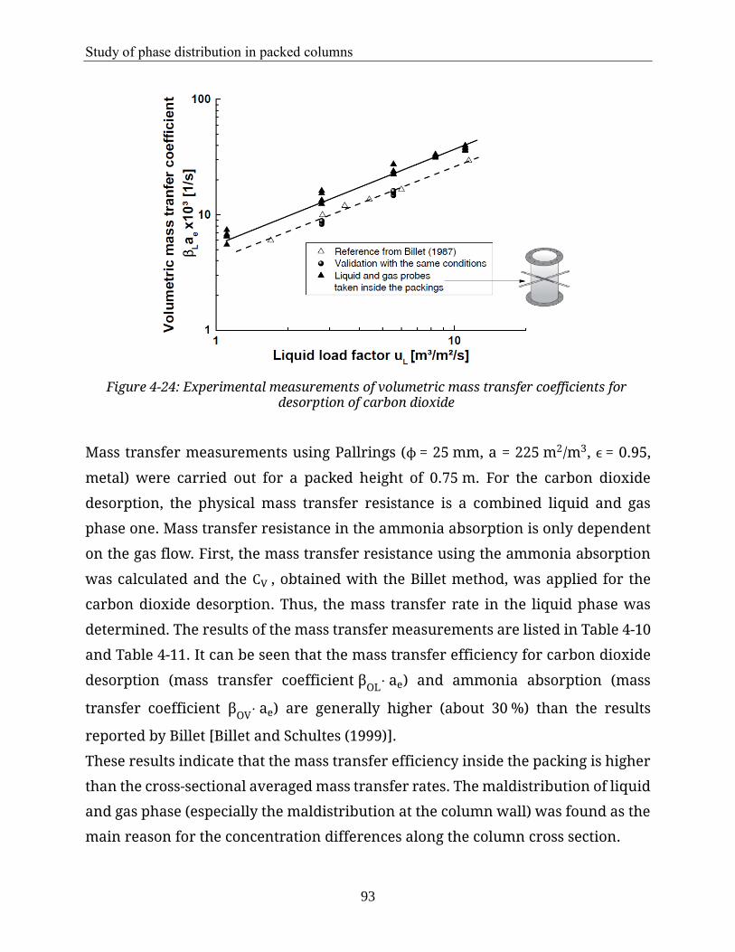
Study of phase distribution in packed columns
93
Figure 4-24: Experimental measurements of volumetric mass transfer coefficients for desorption of carbon dioxide
Mass transfer measurements using Pallrings (ϕ = 25 mm, a = 225 m2/m3, ϵ = 0.95,
metal) were carried out for a packed height of 0.75 m. For the carbon dioxide
desorption, the physical mass transfer resistance is a combined liquid and gas
phase one. Mass transfer resistance in the ammonia absorption is only dependent
on the gas flow. First, the mass transfer resistance using the ammonia absorption
was calculated and the CV , obtained with the Billet method, was applied for the
carbon dioxide desorption. Thus, the mass transfer rate in the liquid phase was
determined. The results of the mass transfer measurements are listed in Table 4-10
and Table 4-11. It can be seen that the mass transfer efficiency for carbon dioxide
desorption (mass transfer coefficient βOL
⋅ ae) and ammonia absorption (mass
transfer coefficient βOV
⋅ ae) are generally higher (about 30 %) than the results
reported by Billet [Billet and Schultes (1999)].
These results indicate that the mass transfer efficiency inside the packing is higher
than the cross-sectional averaged mass transfer rates. The maldistribution of liquid
and gas phase (especially the maldistribution at the column wall) was found as the
main reason for the concentration differences along the column cross section.

Study of phase distribution in packed columns
94
Table 4-10: Experimental measurements of volumetric mass transfer coefficients for
carbon dioxide desorption at different gas and liquid flow rates
Table 4-11: Experimental measurements of volumetric mass transfer coefficients for ammonia absorption at different gas
and liquid flow rates
uL
[m³/m²/h]
FV
[Pa0.5]
CL [-]
HTUOL [-]
HETP [-]
βOL
∙ae
[E³∙1/s]
uL [m³/m²/h]
FV
[Pa0.5]
CL [-]
HTUOL [-]
HETP [-]
βOL
∙ae
[E³∙1/s]
10 0.456 1.740 0.245 1.251 11.338 10 0.404 0.536 0.171 0.472 2.175 10 1.021 1.747 0.244 1.441 11.349 10 1.003 0.520 0.258 0.522 3.588 10 1.450 1.799 0.239 1.489 11.586 10 1.420 0.482 0.318 0.573 4.113 10 1.860 1.957 0.222 1.432 12.512 10 1.731 0.491 0.346 0.579 4.596 10 2.575 1.966 0.223 1.510 12.450 10 2.033 0.533 0.359 0.562 5.195 20 0.713 2.301 0.223 1.087 24.894 20 0.498 0.443 0.157 0.504 2.899 20 0.981 2.175 0.235 1.219 23.609 20 0.988 0.507 0.184 0.479 4.905 20 1.336 2.306 0.223 1.221 24.914 20 1.381 0.472 0.226 0.524 5.602 20 1.677 2.257 0.228 1.299 24.341 20 1.794 0.503 0.244 0.518 6.706 20 2.372 2.391 0.216 1.304 25.664 20 2.050 0.536 0.250 0.507 7.473 30 0.458 1.833 0.310 1.264 26.946 30 0.526 0.434 0.136 0.476 3.552 30 1.015 2.039 0.278 1.345 29.959 30 0.981 0.497 0.153 0.452 5.851 30 1.506 2.063 0.275 1.460 30.271 30 1.508 0.553 0.170 0.443 8.109 30 1.777 2.037 0.279 1.499 29.887 30 1.826 0.562 0.185 0.450 8.998 30 2.008 2.882 0.196 1.076 42.474 30 2.107 0.561 0.198 0.461 9.669 40 0.488 1.965 0.320 1.222 34.852 40 0.472 0.528 0.097 0.372 4.482 40 0.856 1.984 0.317 1.376 35.226 40 0.869 0.606 0.109 0.358 7.303 40 1.356 1.901 0.331 1.584 33.725 40 1.327 0.662 0.120 0.361 10.055 40 1.605 1.967 0.319 1.582 34.891 40 1.545 0.643 0.132 0.378 10.651 40 1.699 2.272 0.268 1.350 41.612 40 1.668 0.667 0.136 0.376 11.173
4.2.2 Experimental investigation of phase distribution using a liquid
collector
Pressure drop and liquid holdup for Pallrings (ϕ = 25 mm, a = 225 m2/m3, ϵ= 0.95,
metal) were measured in packed columns with diameters of ϕ = 288 mm and ϕ =
440 mm. Figure 4-25 shows that the measured pressure drop in both packed
columns is very similar. However, the liquid holdup strongly differs at liquid flow
rates of 30 and 40 m3/m2/h.
These results indicate that the pressure drop is not dependent on the column
diameter at the measured liquid flow rates. Contrary to this, the liquid holdup is
significantly influenced by the column diameter. The reason is that the wall
fraction of a small packed column is higher than that of the larger packed column
and the liquid phase accumulates more easily on the wall of small columns than in
larger columns. Thus, the liquid holdup in small columns is lower. In other words,
maldistribution in smaller columns is much more serious than in larger columns.
It is therefore necessary to study the phase distribution, especially the wall effect,

Study of phase distribution in packed columns
95
in small columns. Following, the phase distribution in ϕ= 288 mm was studied.
Figure 4-25: Experimental measurements of hydrodynamic parameters
The liquid collector shown in Figure 4-26 was applied to measure the liquid flow at
the column wall. The inner diameter of the liquid collector had a smaller diameter
(∅ = 266 mm) than the column, so that the liquid at the column wall was separated
from the rest of the column. Flow rates of the wall liquid were measured at
different gas and liquid loads. The liquid fraction at the column wall in the packed
column, which was filled with Pallrings (25 mm, metal, packed height 2 m), was
measured using the liquid collector. The results are shown in Figure 4-27. It was
seen that at small gas load factors up to 1 Pa0.5 the liquid fraction was relatively
independent on the gas load for all studied liquid flow rates from 5 to 30 m3/m2/h.
Firstly, with an increase of the gas load, the liquid fraction was strongly reduced.
The reason for that was that the gas phase flowing upwards pressed the liquid away
from the inlet range of the liquid collectors. With further increase of the gas load
factor, the liquid fraction on the column wall was strongly increased.
The mass transfer rates of the liquid flowing on the wall were studied using the
liquid collector with ammonia absorption. Air phase with NH3 was blown in from
the bottom of the packed column while liquid phase was distributed by the liquid
distributor from the top of the column. Ammonia concentrations at the gas phase
inlet and outlet were measured.

Study of phase distribution in packed columns
96
Figure 4-26: On-wall liquid collector Figure 4-27: Liquid fraction at the column wall for Pallrings (25 mm, metal) in a packed column (𝜙 =
288 mm) measured with a liquid collector.
NH3 concentration in liquid phase was determined by titration for both, the liquid
that was collected using the liquid collector and the one at the bottom of the packed
column (bulk liquid phase). The ammonia concentration of the on-wall liquid flow
and bulk-phase liquid is illustrated in Figure 4-28.
Measurements 1 to 5 were measured at a liquid flow rate uL of 30 m3/m2/h and gas
loads ug below the flooding point. It is seen that ammonia concentration of the on-
wall liquid phase was much lower than that of the bulk liquid. The ammonia
concentration of the on-wall liquid phase was 3 mol/m3. The ammonia
concentration in the bulk liquid was about 21 mol/m3. These results indicate that
the liquid flowing on the column wall did not effectively participate in the
absorption process.

Study of phase distribution in packed columns
97
Figure 4-28: Study of mass transfer of on-wall liquid using NH3 Absorption
The pressure drop (with gas flow) was further studied with and without the liquid
collector to determine its influence on the accuracy of the measurements. As shown
in Figure 4-29, the depicted lines denote the measurements without liquid collector
while the solid lines denote for the measurements with liquid collector. Higher
pressure drops (about 15 % higher) were generally measured with the liquid
collector at liquid flow rates from 5 to 30 m3/m2/h. This shows that the influence of
liquid collectors on hydrodynamic measurements is considerable.
Figure 4-29: Comparison of pressure drop of Pallrings (25 mm), metal in a packed column (∅ = 288 mm) with and without liquid collector
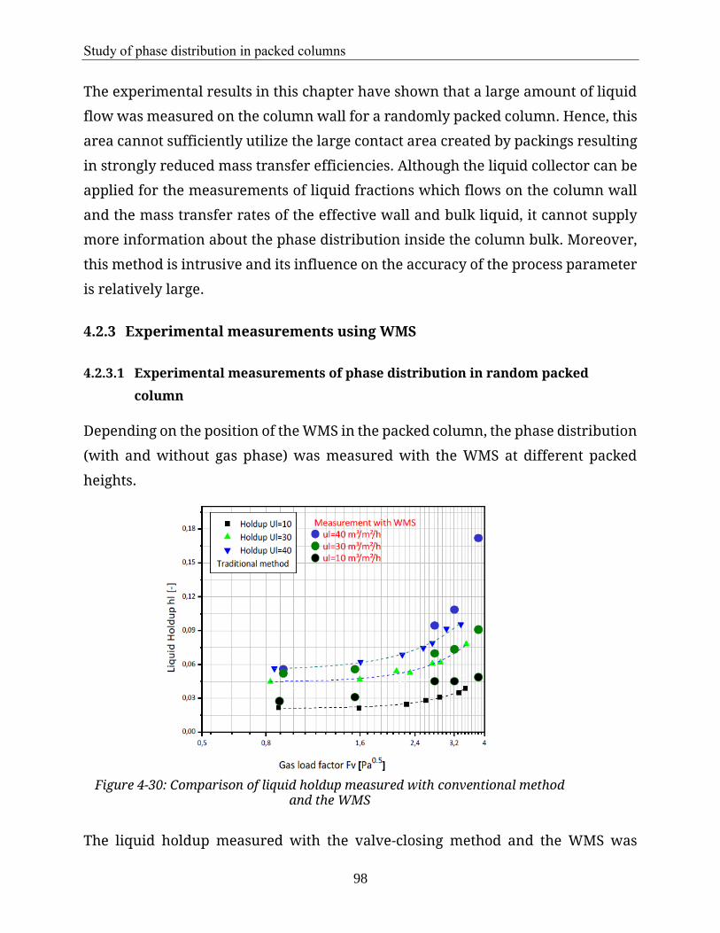
Study of phase distribution in packed columns
98
The experimental results in this chapter have shown that a large amount of liquid
flow was measured on the column wall for a randomly packed column. Hence, this
area cannot sufficiently utilize the large contact area created by packings resulting
in strongly reduced mass transfer efficiencies. Although the liquid collector can be
applied for the measurements of liquid fractions which flows on the column wall
and the mass transfer rates of the effective wall and bulk liquid, it cannot supply
more information about the phase distribution inside the column bulk. Moreover,
this method is intrusive and its influence on the accuracy of the process parameter
is relatively large.
4.2.3 Experimental measurements using WMS
4.2.3.1 Experimental measurements of phase distribution in random packed
column
Depending on the position of the WMS in the packed column, the phase distribution
(with and without gas phase) was measured with the WMS at different packed
heights.
Figure 4-30: Comparison of liquid holdup measured with conventional method
and the WMS
The liquid holdup measured with the valve-closing method and the WMS was

Study of phase distribution in packed columns
99
studied for the Pallring (∅ = 25 mm, a = 225 m2/m3, ϵ = 0.95, metal). The results are
shown in Figure 4-30 for liquid flow rates of 10, 20 and 30 m3/m2/h with counter
current gas flow. The column cross sectional averaged liquid holdup measured by
WMS (circle symbols) was comparable with the liquid holdup (depicted lines)
measured with the valve-closing method. These results indicate that the WMS can
be well used for the determination of the holdup in packed columns.
Phase distribution without gas phase using Pallrings (25 mm, metal) was
experimentally measured and studied with the WMS. The Liquid phase was
distributed from a single point source in the middle of packed column.
The liquid phase distribution at a liquid flow rates of 20 m3/m2/h and packed
heights of 10, 20, 30, 40 and 50 cm is shown in Figure 4-31.
Figure 4-31: Liquid phase distribution in cross-section of packed column at packing height from
10 cm to 50 cm, liquid load factor is 20 m³/m²/h
Liquid phase distribution at different liquid flow rates of 5, 10, 15 and
column diameter[m]
colu
mn
hei
gh
t [c
m]
column diameter[m]

Study of phase distribution in packed columns
100
20 m3/m2/h and packed heights of 10, 20, 30, 40 and 50 cm is shown in Figure 4-32.
It was observed that the maldistribution factor 𝑀𝑓 varied from 0.79 to 0.98 for all
experimental conditions.
(4.32.1) uL = 5 [m³/m²/h],
H = 10 [cm], Mf = 0.98 (4.32.2) uL = 10 [m³/m²/h],
H = 10 [cm], Mf = 0.93 (4.32.3) uL = 15 [m³/m²/h],
H = 10 [cm], Mf = 0.83 (4.32.4) uL=20 [m³/m²/h],
H = 10 [cm], Mf = 0.80
(4.32.5) uL = 5 [m³/m²/h],
H = 20 [cm], Mf = 0.90 (4.32.6) uL = 10 [m³/m²/h],
H = 20 [cm], Mf = 0.89 (4.32.7) uL = 15 [m³/m²/h],
H = 20 [cm], Mf = 0.87 (4.32.8) uL =20 [m³/m²/h],
H = 20 [cm], Mf = 0.85
(4.32.9) uL = 5 [m³/m²/h],
H = 30 [cm], Mf = 0.88 (4.32.10) uL = 10 [m³/m²/h], H =
30 [cm], Mf = 0.86 (4.32.11) uL = 15 [m³/m²/h],
H = 30 [cm], Mf = 0.85 (4.32.12) uL =20 [m³/m²/h],
H = 30 [cm], Mf = 0.84
(4.32.13) uL = 5 [m³/m²/h],
H = 40 [cm], Mf = 0.87 (4.32.14) uL = 10 [m³/m²/h],
H = 40 [cm], Mf = 0.85 (4.32.15) uL = 15 [m³/m²/h],
H = 40 [cm], Mf = 0.83 (4.32.16) uL =20 [m³/m²/h],
H = 40 [cm], Mf = 0.81
(4.32.17) uL = 5 [m³/m²/h],
H = 50 [cm], Mf = 0.86 (4.32.18) uL = 10 [m³/m²/h],
H = 50 [cm], Mf = 0.85 (4.32.19) uL = 15 [m³/m²/h],
H = 50 [cm], Mf = 0.84 (4.32.20) uL =20 [m³/m²/h],
H = 50 [cm], Mf = 0.82
Figure 4-32: Liquid phase distribution in cross-section of packed column at packing height from 10 cm to 50 cm, liquid load factor varies from 5, 10, 15 to 20 m³/m²/h (Black denotes for liquid
phase in cross-section of packed column)

Study of phase distribution in packed columns
101
At a liquid flow rate of 5 m3/m2/h, higher maldistribution factors were determined
for each packed. This is due to the fact that the maldistribution factor was
calculated across the column cross section and the liquid phase mainly
accumulated in the center of the column. The maldistribution factors Mf at a
packed height of 10 cm (Figure 4-32 (4.32.1) to Figure 4-32 (4.32.4)) show relatively
large variances.
The reason is that liquid distribution at the entrance length of the packed column
is strongly influenced by the initial liquid distribution. It was observed that during
the measurements, most of the liquid phase was still flowing as rivulets. With an
increase of the liquid load up to 20 m3/m2/h the maldistribution was slightly
reduced for each studied packed height. These results indicate that the liquid phase
distribution can be slightly influenced by the liquid flow rates for each packed
height. The suggested equations by Cihla who used the diffusion equation to
describe the phase distribution has no dependency of the liquid load. It was
assumed that the liquid load did not influence the phase distribution. However, in
this work was experimentally confirmed that the liquid phase distribution across
the column cross section was slightly influenced by the liquid load. Furthermore, it
was observed that the maldistribution factor Mf at each studied packed height
(from 20 cm to 50 cm) slightly decreases with an increase of packed height. The
phase distribution measured by Mf was almost constant at packed heights of
40 cm and 50 cm and a further increase of the packed height has almost no
influence on the phase distribution.
The liquid holdup in the radial direction (values were averaged over 10 seconds) is
shown in Figure 4-33 for packed heights of 10 cm and 20 cm. Blue marks were
measurements at 5 m3/m2/h (fitted by the blue line), red marks were measurements
at 10 m3/m2/h (fitted by the black line) and black marks were measurements at
15 m3/m2/h (fitted by the red line). For the measurements using Pallrings (without
gas phase), it can be seen that the liquid distributed in the radial range of 6 cm for
all studied cases (different packed heights and liquid loads).
The countercurrent gas flow, can strongly influence the distribution. Therefore, the
packed height of 10 cm was used to study the gas phase influence on the liquid
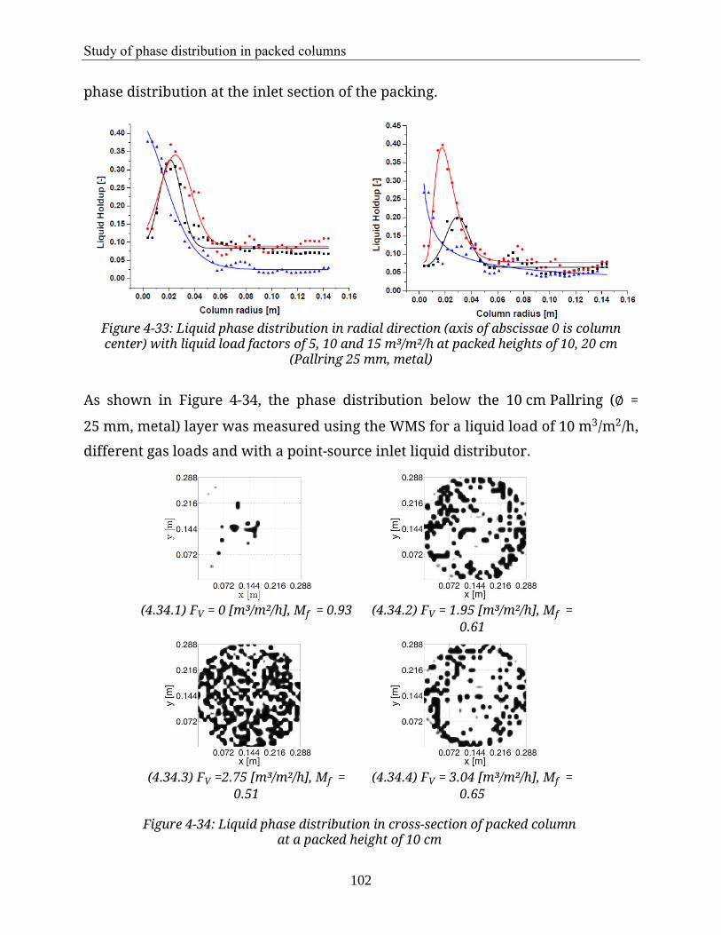
Study of phase distribution in packed columns
102
phase distribution at the inlet section of the packing.
Figure 4-33: Liquid phase distribution in radial direction (axis of abscissae 0 is column center) with liquid load factors of 5, 10 and 15 m³/m²/h at packed heights of 10, 20 cm
(Pallring 25 mm, metal)
As shown in Figure 4-34, the phase distribution below the 10 cm Pallring (∅ =
25 mm, metal) layer was measured using the WMS for a liquid load of 10 m3/m2/h,
different gas loads and with a point-source inlet liquid distributor.
(4.34.1) FV = 0 [m³/m²/h], Mf = 0.93 (4.34.2) FV = 1.95 [m³/m²/h], Mf =
0.61
(4.34.3) FV =2.75 [m³/m²/h], Mf =
0.51
(4.34.4) FV = 3.04 [m³/m²/h], Mf =
0.65
Figure 4-34: Liquid phase distribution in cross-section of packed column at a packed height of 10 cm
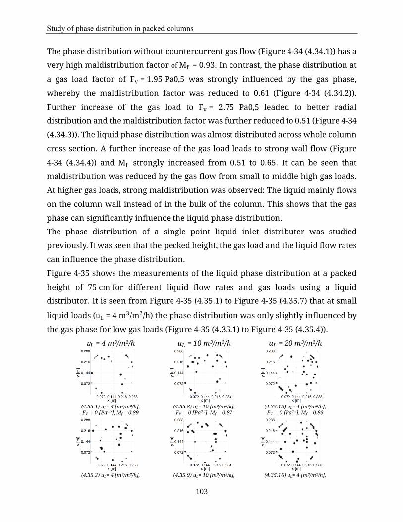
Study of phase distribution in packed columns
103
The phase distribution without countercurrent gas flow (Figure 4-34 (4.34.1)) has a
very high maldistribution factor of Mf = 0.93. In contrast, the phase distribution at
a gas load factor of Fv = 1.95 Pa0,5 was strongly influenced by the gas phase,
whereby the maldistribution factor was reduced to 0.61 (Figure 4-34 (4.34.2)).
Further increase of the gas load to Fv = 2.75 Pa0,5 leaded to better radial
distribution and the maldistribution factor was further reduced to 0.51 (Figure 4-34
(4.34.3)). The liquid phase distribution was almost distributed across whole column
cross section. A further increase of the gas load leads to strong wall flow (Figure
4-34 (4.34.4)) and Mf strongly increased from 0.51 to 0.65. It can be seen that
maldistribution was reduced by the gas flow from small to middle high gas loads.
At higher gas loads, strong maldistribution was observed: The liquid mainly flows
on the column wall instead of in the bulk of the column. This shows that the gas
phase can significantly influence the liquid phase distribution.
The phase distribution of a single point liquid inlet distributer was studied
previously. It was seen that the pecked height, the gas load and the liquid flow rates
can influence the phase distribution.
Figure 4-35 shows the measurements of the liquid phase distribution at a packed
height of 75 cm for different liquid flow rates and gas loads using a liquid
distributor. It is seen from Figure 4-35 (4.35.1) to Figure 4-35 (4.35.7) that at small
liquid loads (uL = 4 m3/m2/h) the phase distribution was only slightly influenced by
the gas phase for low gas loads (Figure 4-35 (4.35.1) to Figure 4-35 (4.35.4)).
uL = 4 m³/m²/h uL = 10 m³/m²/h uL = 20 m³/m²/h
(4.35.1) uL= 4 [m³/m²/h], FV = 0 [Pa0.5], Mf = 0.89
(4.35.8) uL= 10 [m³/m²/h], FV = 0 [Pa0.5], Mf = 0.87
(4.35.15) uL= 4 [m³/m²/h], FV = 0 [Pa0.5], Mf = 0.83
(4.35.2) uL= 4 [m³/m²/h], (4.35.9) uL= 10 [m³/m²/h], (4.35.16) uL= 4 [m³/m²/h],

Study of phase distribution in packed columns
104
FV = 1.11 [Pa0.5], Mf = 0.88 FV = 1.11 [Pa0.5], Mf = 0.86 FV = 1.11 [Pa0.5], Mf = 0.83
(4.35.3) uL= 4 [m³/m²/h],
FV = 1.41 [Pa0.5], Mf = 0.87 (4.35.10) uL= 10 [m³/m²/h], FV = 1.41 [Pa0.5], Mf = 0.85
(4.35.17) uL=20 [m³/m²/h], FV = 1.41 [Pa0.5], Mf = 0.83
(4.35.4) uL= 4 [m³/m²/h],
FV = 2.0 [Pa0.5], Mf = 0.86 (4.35.11) uL= 10 [m³/m²/h], FV = 2.0 [Pa0.5], Mf = 0.83
(4.35.18) uL= 20 [m³/m²/h], FV = 2.0 [Pa0.5], Mf = 0.81
(4.35.5) uL= 4 [m³/m²/h],
FV = 2.84 [Pa0.5], Mf = 0.77 (4.35.12) uL= 10 [m³/m²/h], FV = 2.84 [Pa0.5], Mf = 0.80
(4.35.19) uL= 20 [m³/m²/h], FV = 2.84 [Pa0.5], Mf = 0.77
(4.35.6) uL= 4 [m³/m²/h],
FV = 3.40 [Pa0.5], Mf = 0.74 (4.35.13) uL= 10 [m³/m²/h], FV = 3.40 [Pa0.5], Mf = 0.71
(4.35.20) uL= 20 [m³/m²/h], FV = 3.40 [Pa0.5], Mf = 0.73
(4.35.7) uL= 4 [m³/m²/h],
FV = 3.80 [Pa0.5], Mf = 0.77
(4.35.14) uL= 10 [m³/m²/h], FV = 3.80 [Pa0.5], Mf = 0.69
(4.35.21) uL= 20 [m³/m²/h], FV = 3.80 [Pa0.5], Mf = 0.71
Figure 4-35: Liquid phase distribution in cross-section of packed column with
liquid distributor at different liquid flow rates
With an increase of the gas load (Figure 4-35 (4.35.5) to Figure 4-35 (4.35.7)), the
liquid phase strongly accumulated at the column wall. Similar effects were seen for

Study of phase distribution in packed columns
105
the liquid load of uL = 10 m3/m2/h (see Figure 4-35 (4.35.8) to Figure 4-35 (4.35.14))
and 20 m3/m2/h (see Figure 4-35 (4.35.9) to (4.35.27)). Although at higher liquid
loads the liquid phase distributed more uniformly across the whole cross section,
the liquid flowed preferably near the column wall. Thus, it can be concluded that
the liquid phase maldistribution in the random packing is relatively high and the
gas phase can lead to strong accumulation of the liquid at the wall depending on
the gas as well as the liquid loads.
Figure 4-36 illustrates the dynamic phase distribution of Pallrings across the
column cross section measured by the WMS. The liquid flow on the column wall
was present mainly as film flow, which was stable over time. Within the column
bulk, most of the observed liquid was identified as droplets. The liquid flowing on
the column wall is not effective for mass transfer which was experimentally
determined and discussed during the mass transfer measurements.
Thus, it can be concluded that the separation efficiency in random packed columns
is strongly influenced by the liquid maldistribution on the column wall which itself
is strongly influenced by the gas load. Although in the loading range of the packed
column, the turbulence of liquid phase can facilitate the mass transfer, the fraction
of the liquid phase on the column wall is high and its influence cannot be neglected
for random packings.
Figure 4-36: Dynamic phase distribution across the column cross section (green and red denote for liquid phase)
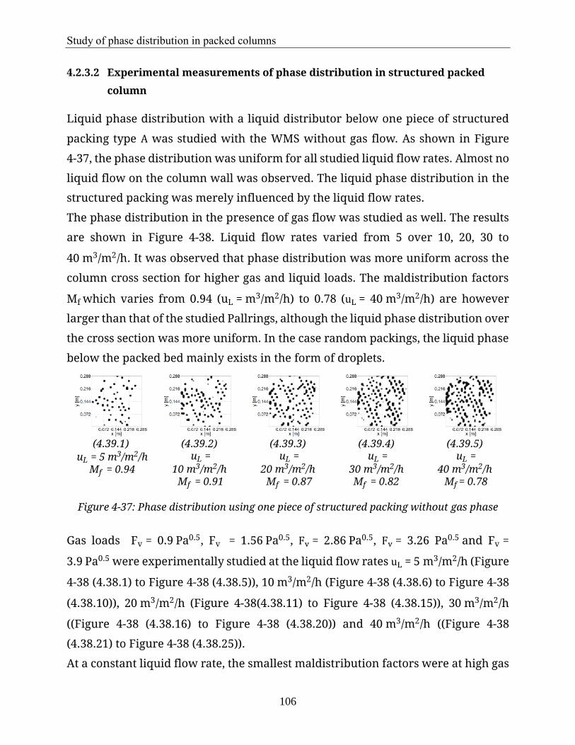
Study of phase distribution in packed columns
106
4.2.3.2 Experimental measurements of phase distribution in structured packed
column
Liquid phase distribution with a liquid distributor below one piece of structured
packing type A was studied with the WMS without gas flow. As shown in Figure
4-37, the phase distribution was uniform for all studied liquid flow rates. Almost no
liquid flow on the column wall was observed. The liquid phase distribution in the
structured packing was merely influenced by the liquid flow rates.
The phase distribution in the presence of gas flow was studied as well. The results
are shown in Figure 4-38. Liquid flow rates varied from 5 over 10, 20, 30 to
40 m3/m2/h. It was observed that phase distribution was more uniform across the
column cross section for higher gas and liquid loads. The maldistribution factors
Mf which varies from 0.94 (uL = m3/m2/h) to 0.78 (uL = 40 m3/m2/h) are however
larger than that of the studied Pallrings, although the liquid phase distribution over
the cross section was more uniform. In the case random packings, the liquid phase
below the packed bed mainly exists in the form of droplets.
(4.39.1)
uL = 5 m3/m2/h Mf = 0.94
(4.39.2) uL =
10 m3/m2/h Mf = 0.91
(4.39.3) uL =
20 m3/m2/h Mf = 0.87
(4.39.4) uL =
30 m3/m2/h Mf = 0.82
(4.39.5) uL =
40 m3/m2/h Mf = 0.78
Figure 4-37: Phase distribution using one piece of structured packing without gas phase
Gas loads Fv = 0.9 Pa0.5, Fv = 1.56 Pa0.5, Fv = 2.86 Pa0.5, Fv = 3.26 Pa0.5 and Fv =
3.9 Pa0.5 were experimentally studied at the liquid flow rates uL = 5 m3/m2/h (Figure
4-38 (4.38.1) to Figure 4-38 (4.38.5)), 10 m3/m2/h (Figure 4-38 (4.38.6) to Figure 4-38
(4.38.10)), 20 m3/m2/h (Figure 4-38(4.38.11) to Figure 4-38 (4.38.15)), 30 m3/m2/h
((Figure 4-38 (4.38.16) to Figure 4-38 (4.38.20)) and 40 m3/m2/h ((Figure 4-38
(4.38.21) to Figure 4-38 (4.38.25)).
At a constant liquid flow rate, the smallest maldistribution factors were at high gas

Study of phase distribution in packed columns
107
loads (e.g. Fv = 3.26 Pa0.5or Fv = 3.9 Pa0.5). The liquid phase distribution at lower gas
flow rates showed better distribution patterns than that of Pallrings (25 mm,
metal). Moreover, there was measured almost no large-scale maldistribution. The
reason is that the influence of gas flow on the liquid flow is limited by the structure
of the packings. The free volume between the structured packing and the column
wall was much smaller than for the random packings. Thus, based on these
experimental results it can be concluded that large scale maldistribution mainly
occurs in randomly packed columns.
4.3 Simulation and Modeling of phase distribution
In order to predict the hydrodynamics and mass transfer processes in packed
columns more accurately, numerous attempts have been applied to model both
these processes. Among these models, two main categories can be summarized: the
volume-averaged methods (e.g. Billet method) and geometry-based methods (e.g.
CFD methods). Both methods have its drawbacks: the local phase distribution,
especially maldistribution is not considered in the volume-averaged models and
the phase distribution in random packed columns is difficult to simulate using CFD
for the whole column due to the computational effort.
uL = 5 [m3/m2/h]
uL = 10 [m3/m2/h]
uL = 20 [m3/m2/h]
uL = 30 [m3/m2/h]
uL = 40 [m3/m2/h]
Fv = 0.90 [Pa0.5],
Mf = 0.94 Fv = 0.90 [Pa0.5],
Mf = 0.85 Fv = 0.90 [Pa0.5],
Mf = 0.78 Fv = 0.90 [Pa0.5],
Mf = 0.81 Fv = 0.90 [Pa0.5],
Mf = 0.77
Fv = 1.56 [Pa0.5],
Mf = 0.94 Fv = 1.56 [Pa0.5],
Mf = 0.89 Fv = 1.56 [Pa0.5],
Mf = 0.78 Fv = 1.56 [Pa0.5],
Mf = 0.80 Fv = 1.56 [Pa0.5],
Mf = 0.68
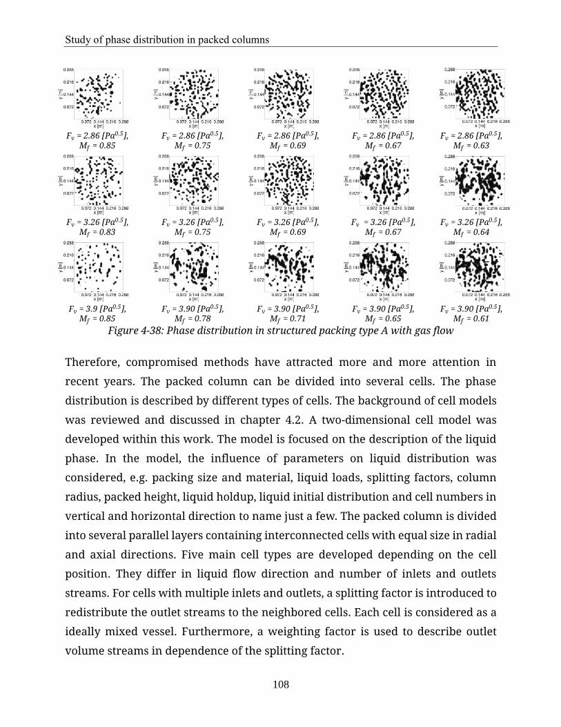
Study of phase distribution in packed columns
108
Fv = 2.86 [Pa0.5],
Mf = 0.85 Fv = 2.86 [Pa0.5],
Mf = 0.75 Fv = 2.86 [Pa0.5],
Mf = 0.69 Fv = 2.86 [Pa0.5],
Mf = 0.67 Fv = 2.86 [Pa0.5],
Mf = 0.63
Fv = 3.26 [Pa0.5],
Mf = 0.83 Fv = 3.26 [Pa0.5],
Mf = 0.75 Fv = 3.26 [Pa0.5],
Mf = 0.69 Fv = 3.26 [Pa0.5],
Mf = 0.67 Fv = 3.26 [Pa0.5],
Mf = 0.64
Fv = 3.9 [Pa0.5],
Mf = 0.85 Fv = 3.90 [Pa0.5],
Mf = 0.78 Fv = 3.90 [Pa0.5],
Mf = 0.71 Fv = 3.90 [Pa0.5],
Mf = 0.65 Fv = 3.90 [Pa0.5],
Mf = 0.61 Figure 4-38: Phase distribution in structured packing type A with gas flow
Therefore, compromised methods have attracted more and more attention in
recent years. The packed column can be divided into several cells. The phase
distribution is described by different types of cells. The background of cell models
was reviewed and discussed in chapter 4.2. A two-dimensional cell model was
developed within this work. The model is focused on the description of the liquid
phase. In the model, the influence of parameters on liquid distribution was
considered, e.g. packing size and material, liquid loads, splitting factors, column
radius, packed height, liquid holdup, liquid initial distribution and cell numbers in
vertical and horizontal direction to name just a few. The packed column is divided
into several parallel layers containing interconnected cells with equal size in radial
and axial directions. Five main cell types are developed depending on the cell
position. They differ in liquid flow direction and number of inlets and outlets
streams. For cells with multiple inlets and outlets, a splitting factor is introduced to
redistribute the outlet streams to the neighbored cells. Each cell is considered as a
ideally mixed vessel. Furthermore, a weighting factor is used to describe outlet
volume streams in dependence of the splitting factor.

Study of phase distribution in packed columns
109
4.3.1 Cell model
The packed column was divided into parallel layers and each layer contained a
certain number of interconnected cells (see Figure 4-39).
Figure 4-39: Two-dimensional symmetric cell model
Since the phase distribution in cylindrical coordinate depends on the column
radius 𝑟 and the packed height Z, the model was simplified as a symmetrical two-
dimensional model in Cartesian coordinates.
The connections of the cells for a M×N model are illustrated in Figure 4-40.
Figure 4-40: Two-dimensional symmetric cell model with liquid inlet and outlet steams
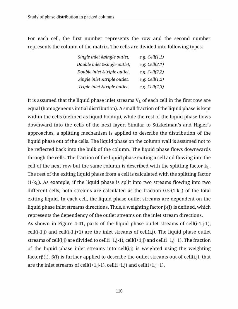
Study of phase distribution in packed columns
110
For each cell, the first number represents the row and the second number
represents the column of the matrix. The cells are divided into following types:
Single inlet &single outlet, e.g. Cell(1,1)
Double inlet &single outlet, e.g. Cell(2,1)
Double inlet &triple outlet, e.g. Cell(2,2)
Single inlet &triple outlet, e.g. Cell(1,2)
Triple inlet &triple outlet, e.g. Cell(2,3)
It is assumed that the liquid phase inlet streams VL of each cell in the first row are
equal (homogeneous initial distribution). A small fraction of the liquid phase is kept
within the cells (defined as liquid holdup), while the rest of the liquid phase flows
downward into the cells of the next layer. Similar to Stikkelman’s and Higler’s
approaches, a splitting mechanism is applied to describe the distribution of the
liquid phase out of the cells. The liquid phase on the column wall is assumed not to
be reflected back into the bulk of the column. The liquid phase flows downwards
through the cells. The fraction of the liquid phase exiting a cell and flowing into the
cell of the next row but the same column is described with the splitting factor kL.
The rest of the exiting liquid phase from a cell is calculated with the splitting factor
(1-kL). As example, if the liquid phase is split into two streams flowing into two
different cells, both streams are calculated as the fraction 0.5⋅(1-kL) of the total
exiting liquid. In each cell, the liquid phase outlet streams are dependent on the
liquid phase inlet streams directions. Thus, a weighting factor β(i) is defined, which
represents the dependency of the outlet streams on the inlet stream directions.
As shown in Figure 4-41, parts of the liquid phase outlet streams of cell(i-1,j-1),
cell(i-1,j) and cell(i-1,j+1) are the inlet streams of cell(i,j). The liquid phase outlet
streams of cell(i,j) are divided to cell(i+1,j-1), cell(i+1,j) and cell(i+1,j+1). The fraction
of the liquid phase inlet streams into cell(i,j) is weighted using the weighting
factorβ(i). β(i) is further applied to describe the outlet streams out of cell(i,j), that
are the inlet streams of cell(i+1,j-1), cell(i+1,j) and cell(i+1,j+1).

Study of phase distribution in packed columns
111
Figure 4-41: Cell type inside packings
The weighting factor β(i) is calculated using (eq. 4-66), (eq. 4-67) and (eq. 4-68).
β1 =
V.
c(i-1,j),out1
V.
c(i,j),in
⋅kL
V.
c(i-1,j-1),out2
V.
c(i,j),in
⋅0.5(1-kL)+V.
c(i-1,j),out1
V.
c(i,j),in
⋅kL+V.
c(i-1,j+1),out3
V.
c(i,j),in
⋅0.5(1-kL)
(eq. 4-66)
β2 =
V.
c(i-1,j-1),out2
V.
c(i,j),in
⋅0.5(1-kL)
V.
c(i-1,j-1),out2
V.
c(i,j),in
⋅0.5(1-kL)+V.
c(i-1,j),out1
V.
c(i,j),in
⋅kL+V.
c(i-1,j+1),out3
V.
c(i,j),in
⋅0.5(1-kL)
(eq. 4-67)
β 3
=
V.
c(i-1,j+1),out3
V.
c(i,j),in
⋅0.5(1-kL)
V.
c(i-1,j-1),out2
V.
c(i,j),in
⋅0.5(1-kL)+V.
c(i-1,j),out1
V.
c(i,j),in
⋅kL+V.
c(i-1,j+1),out3
V.
c(i,j),in
⋅0.5(1-kL)
(eq. 4-68)
whereby β1is the weighting factor into the vertical cell of the next layer and β
2 and
β3 are the weighting factors of the left and right neighbored cells to central cell of
the next layer, respectively. The liquid phase inlet stream V.
c(i,j),in of cell(i,j) is the
sum of the liquid phase outlet streams of cell(i+1,j-1), cell(i+1,j) and cell(i+1,j+1):
V.
c(i,j),in = V.
c(i-1,j-1),out1+V.
c(i-1,j),out2+V.
c2(i-1,j+1),out3 (eq. 4-69)
The liquid phase inlets streams of cell(i+1,j-1), cell(i+1,j) and cell(i+1,j+1) depend on
the splitting factors β(i) of cell(i,j) and are described as:

Study of phase distribution in packed columns
112
V.
c(i,j),out1 = β1
⋅V.
c(i,j),in (eq. 4-70)
V.
c(i,j),out2=β2
⋅V.
c(i,j),in (eq. 4-71)
V.
c(i,j),out3=β3
⋅V.
c(i,j),in (eq. 4-72)
Depending on the cell position in the packed columns, various cell types are applied
in the cell model. On the first layer two types of cells are used: The first and the last
cell on the first layer are the same cell type (cells assumed as lying on the column
wall) and shown in Figure 4-42 a). The cell on the first layer, cell(1,1) and cell(1,N),
contains a single input stream and a single outlet stream. Cells between the first
and the last cell have a single inlet stream and three outlet streams (shown in
Figure 4-42 b).
a) Cells at the column wall in the first layer
b) Bulk cells in the first layer
Figure 4-42: Cell types for the initial liquid phase inlet layer
Beginning from the second layer, there are three types of cells:
1) The cells(i,1) (i ≥ 2) (cells on the column wall) receives two inlet streams from
above cells outlet flows, which are from cell(i-1,1) and cell(i-1,2), while
cell(i,N) (I ≥ 2) receives two inlet streams from above cells. Which areoutlet
flows from cell(i-1,N-1) and cell(i-1,N) (shown in Figure 4-43). The liquid
phase outlet streams of cell(i,1) and cell(i,N) are inlet streams of cell(i+1,1)
and cell(i+1,N), respectively. No splitting factors were needed for this cell
type since the liquid phase on the column wall is assumed not to be reflected
back into the packing.

Study of phase distribution in packed columns
113
Figure 4-43: Cell type a) since second layer
2) The cell(i,2) (i ≥ 2) (shown in Figure 4-44) receives two inlet streams from
above cells, which are outlet flows from cell(i-1,2) and cell(i-1,3), while
cell(i,N-1) (i ≥ 2) receives two inlet streams from above cells, which areoutlet
flows from cell(i-1,N-2) and cell(i-1,N-1). The liquid phase outlet streams of
cell(i,1)/cell(i,N) are inlet streams of cell(i+1,1), cell(i+1,2) and
cell(i+1,3)/cell(i+1,N-2), cell(i+1,N-1) and cell(i+1,N), respectively.
Figure 4-44: Cell type b) since second layer
The splitting factors β(i) for the outlet streams of cell(i,2) (i ≥ 2) are defined as:

Study of phase distribution in packed columns
114
β1=
V.
c(i-1,2),out1
V.
c(i,2),in
⋅kL
V.
c(i-1,1),out3
V.
c(i,2),in
⋅(1-kL)+V.
c(i-1,2),out1
V.
c(i,2),in
⋅kL
(eq. 4-73)
β2=
V.
c(i-1,2),out1
V.
c(i,2),in
⋅(1-γ)(1-kL)
V.
c(i-1,2),out3
V.
c(i,1),in
⋅(1-kL)+V.
c(i-1,2),out1
V.
c(i,2),in
⋅kL
(eq. 4-74)
β3=
V.
c(i-1,1),out3
V.
c(i,2),in
⋅γ(1-kL)
V.
c(i-1,1),out3
V.
c(i,2),in
⋅(1-kL)+V.
c(i-1,2),out1
V.
c(i,2),in
⋅kL
(eq. 4-75)
The factor γ is defined to describe the outlet streams of cell(i,2). Therefore, γ is
adjusted and fitted depending on the packing characteristics. The liquid phase
outlet streams of cell(i,2) are described by using the splitting factors β(i) for (eq.
4-76) to (eq. 4-79).
V.
c(i,2),in=V.
c(i-1,2),out1+V.
c(i-1,1),out3 (eq. 4-76)
V.
c(i,2),out1=β1
⋅x⋅V.
c(i,2),in (eq. 4-77)
V.
c(i,2),out2=β2
⋅x⋅V.
c(i,2),in (eq. 4-78)
V.
c(i,2),out3=β3
⋅x⋅V.
c(i,2),in (eq. 4-79)
Similar to cell(i,2) (i ≥ 2), the splitting factors β(i) for the outlet streams of cell(i,N-2)
((i ≥2) are defined as following:
β1=
V.
c(i-1,N-1),out1
V.
c(i,N-1),in
⋅kL
V.
c(i-1,N-2),out3
V.
c(i,N-1),in
⋅(1-kL)+V.
c(i-1,N-1),out1
V.
c(i,N-1),in
⋅kL
(eq. 4-80)
𝛽2 =
𝑉.
𝑐(𝑖−1,𝑁−1),𝑜𝑢𝑡1
𝑉.
𝑐(𝑖,𝑁−1),𝑖𝑛
⋅ (1 − 𝛾)(1 − 𝑘𝐿)
𝑉.
𝑐(𝑖−1,𝑁−1),𝑜𝑢𝑡3
𝑉.
𝑐(𝑖,𝑁−2),𝑖𝑛
⋅ (1 − 𝑘𝐿) +𝑉.
𝑐(𝑖−1,𝑁−1),𝑜𝑢𝑡1
𝑉.
𝑐(𝑖,𝑁−1),𝑖𝑛
⋅ 𝑘𝐿
(eq. 4-81)

Study of phase distribution in packed columns
115
β3=
V.
c(i-1,N-2),out3
V.
c(i,N-1),in
⋅γ(1-kL)
V.
c(i-1,N-2),out3
V.
c(i,N-1),in
⋅(1-kL)+V.
c(i-1,N-1),out1
V.
c(i,N-1),in
⋅kL
(eq. 4-82)
Whereby the factor γ is defined to weight the outlet streams of cell(i,N-1). The liquid
phase outlet streams of cell(i,N-1) are described using the splitting factors β(i) for
(eq. 4-83) to (eq. 4-86).
V.
c(i,N-1),in=V.
c(i-1,N-1),out1+V.
c(i-1,N-2),out3 (eq. 4-83)
V.
c(i,N-1),out1=β1
⋅x⋅V.
c(i,N-1),in (eq. 4-84)
V.
c(i,N-1),out2=β2
⋅x⋅V.
c(i,N-1),in (eq. 4-85)
V.
c(i,N-1),out3=β3
⋅x⋅V.
c(i,N-1),in (eq. 4-86)
3) The third cell type (with 3 inlet streams and 3 outlet streams) is shown in Figure
4-41 and the corresponding splitting factors β(i) were already described in (eq.
4-66) to (eq. 4-72). This cell type is used for the bulk cells which are not directly
influenced by the column wall.
Every cell illustrated in Figure 4-40 is assumed as an ideally stirred tank. Its
temporal change of the liquid holdup depends on the number of liquid inlets and
outlets streams in the consideration of the corresponding splitting factors.
Δholdup
Δtime = ∑(liquid inlet streams from upper layer) –
∑(liquid outlet streams to lower layer)
(eq. 4-87)
The outlet streams are dependent on the liquid holdup of each cell. After a short
unsteady simulation (δholdup/δt≠0), an equilibrium state is reached, whereby the
liquid cell holdups are not dependent on the simulation time anymore.
Liquid distribution is simulated with and without the weighting factors. In the case
of model without the weighting factors, the cells are assumed as well stirred tanks
and the outlet streams out of every cell are not dependent on the direction of the
inlet streams. The streams only depend on the defined splitting factors. In the
model with weighting factors the outlet streams of each cell are weighted according
to the amount and direction of the inlet streams. This means, if the amount of inlet

Study of phase distribution in packed columns
116
stream in one direction is much larger than the one in other directions, the outlet
streams in that direction are also larger. It should be noted that the weighting factor
should be determined based on experimental studies or fitted to experimental
measurements.
4.3.2 Simulation of phase distribution using cell model
The cell model described previously was simulated in MATLAB. The liquid
distribution was studied for a point source central inlet. Unsteady-state equations
(solved with ode45 function of MATLAB) were applied. The phase distribution is a
function of time and the temporal holdup was calculated in each cell. Steady state
was reached when the holdup was not dependent on time anymore. It was
observed that the steady-state in each cell can be obtained really quickly.
By parameter analysis of the phase distribution it was found that the cell number
in vertical and horizontal direction as well as the splitting factor most significantly
influenced the phase distribution. The packing height was not directly influencing
the phase distribution for the investigated cell numbers. Liquid flow rates and the
value of the liquid holdup did not influence the phase distribution.
As shown in Figure 4-45 and Figure 4-46, the random packed column (shown in
Figure 4-39) was divided into 10×10 and 18×18 cells, individually. The splitting
factor was varied from 0.1 to 0.4 with the same averaged liquid amount in each cell
assumed as 3 %.

Study of phase distribution in packed columns
117
a) splitting factor = 0.1 b) splitting factor = 0.2
c) splitting factor = 0.3 d) splitting factor = 0.4
Figure 4-45: Simulation results using cell model with 10×10 cells
Compared to the simulation with 18×18 cells, the 10×10 cell model denotes for large
packings. For the 10x10 simulation, it is seen in Figure 4-45 that for splitting factors
larger than 0.2 the liquid reaches the column wall.
For 18×18 cells, the liquid phase reaches the column wall for splitting factors larger
than 0.3. This means that larger packings lead the liquid more easily to the wall
than smaller packings.
a) splitting factor = 0.1 b) splitting factor = 0.2

Study of phase distribution in packed columns
118
c) splitting factor = 0.3 d) splitting factor = 0.4
Figure 4-46: Simulation results using cell model with 18×18 cells
In Figure 4-45 d) and Figure 4-46 d) it is shown that the liquid phase accumulates
on the column wall and its amount increases continuously with increasing packed
height. This assumption was realized in the cell model because it is based on the
experimental observations. The liquid phase on the column wall cannot be
redistributed back into the column bulk.
Next, the splitting factor was set as 0.3 for a 13×13 cell model. The liquid inlet was
assumed as centered and homogeneous. It is seen in Figure 4-47 that a significant
amount of the liquid fraction was observed on the column wall at homogeneous
liquid inlet conditions.
Other factors influencing the liquid phase distribution are either not significant
(e.g., local liquid amount held in the cells) or can be summarized in the liquid
splitting factor (gas phase upwards enlarged the liquid distribution, thus leading to
a larger splitting factor). The liquid flow rates is influencing the absolute liquid
holdup values but is not significantly influencing the liquid distribution.
Furthermore, the influence of cell number on liquid phase distribution was
studied. It was found that the cell number can influence the amount of liquid on
the column wall.
Splitting factors should be experimentally determined using the single point liquid

Study of phase distribution in packed columns
119
inlet source. The fitted splitting factor can then be used for a homogeneous liquid
inlet. It should be noted that in this model it was assumed that the splitting factor
was constant and independent of cell position. In reality, the splitting factor
strongly depends on the arrangement of the random packings.
Figure 4-47: Phase distribution for a splitting factor of 0.3 using a 13×13 cell model
4.4 Discussion
In this chapter the topic of packed columns was reviewed. Volume-averaged
models, e.g. the widely cited and used film model proposed by Billet was
experimental proved as an effective method to evaluate the hydrodynamic and
mass transfer parameters for random and structured packings. Advantages of this
method is that a large amount of experimental measurements were applied for
derivation of the equations. Especially, mass transfer processes were well
described by rate-based model. Based on the experimental measurements, some
limitations of the Billet method were found.
Moreover, the phase distribution in packed column was experimentally studied.
Phase distribution is an important factor which determines the efficiency of the
packed column. The phase distribution was experimentally studied using a
modified conventional method and the WMS method which has been discussed in
a previous chapter. The influence of the conventional method was experimentally
Study of phase distribution in packed columns
120
studied, and it was seen that the measuring method is very intrusive and can
strongly influence the results making the measurements less reliable. With the aid
of the capacitive WMS, the phase distribution was experimentally measured. A
large-scale liquid maldistribution, namely liquid wall flow was identified in
random packed columns.
Finally, the phase distribution, especially the liquid fraction of wall flow, was
described using the cell model. It was seen that some parameters, e.g. the splitting
factor, the cell number and the liquid exchange between cells have noticeable
influences on the phase distribution.
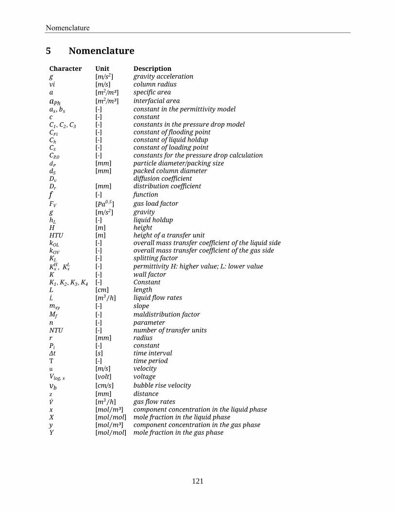
Nomenclature
121
5 Nomenclature
Character Unit Description g [m/s2] gravity acceleration vi [m/s] column radius a [m2/m³] specific area
aPh [m2/m³] interfacial area
ax, bx [-] constant in the permittivity model c [-] constant C1, C2, C3 [-] constants in the pressure drop model C𝐹𝑙 [-] constant of flooding point Ch [-] constant of liquid holdup C𝑆 [-] constant of loading point CP,0 [-] constants for the pressure drop calculation 𝑑𝑃 [mm] particle diameter/packing size dS [mm] packed column diameter Dv diffusion coefficient Dr [mm] distribution coefficient
f [-] function
FV [Pa0.5] gas load factor
g [m/s2] gravity hL [-] liquid holdup H [m] height HTU [m] height of a transfer unit kOL [-] overall mass transfer coefficient of the liquid side kOV [-] overall mass transfer coefficient of the gas side KL [-] splitting factor
KxH
, KxL [-] permittivity H: higher value; L: lower value
K [-] wall factor K1, K2, K3, K4 [-] Constant L [cm] length
�� [m3 h⁄ ] liquid flow rates mxy [-] slope
Mf [-] maldistribution factor
n [-] parameter NTU [-] number of transfer units r [mm] radius Pi [-] constant Δt [s] time interval T [-] time period u [m/s] velocity Vlog, x [volt] voltage
vb [cm/s] bubble rise velocity
z [mm] distance
�� [m3 h⁄ ] gas flow rates x [mol m³⁄ ] component concentration in the liquid phase X [mol mol⁄ ] mole fraction in the liquid phase y [mol m³⁄ ] component concentration in the gas phase Y [mol mol⁄ ] mole fraction in the gas phase

Nomenclature
122
Symbol
φ [mm] diameter
ψ [-] resistance coefficient
μ [-] packing type dependent factor
τ [s] residence time
𝜓𝑥𝑦 [-] function
ε [-] porosity
ρ [kg/m³] density
β1 , β
2 , β
3 [-] splitting factor in the cell model
v [m/s] velocity
σ [N/m] surface tension
ϵ [-] packing porosity
ξ [-] resistance coefficient
δ [mm] thickness
θ [°] angle
η [Pa/s] dynamic viscosity
λ0 [-] mass flow ratio of the gas-liquid phase
β [m³/m²/s] mass transfer coefficient
ML [g/mol] mole weight of the liquid phase
MV [g/mol] mole weight of the gas phase
Subscript
V gas/bubble
P pressure
L liquid
0 un-wetted
VL gas and liquid phase
S loading point
FL flooding point
Superscript
i integer
j integer
n stage number
Ph interfacial
Dimensionless number
Re [-] Reynolds number
We [-] Weber number
Fr [-] Froude number
Sc [-] Schmidt number
Sh [-] Sherwood number

References
123
6 References
[Abdulkadir et al. (2014)] Abdulkadir, M., V. Hernandez-Perez, I. Lowndes, B. Azzopardi, and E. Brantson (2014). Detailed analysis of phase distributions in a vertical riser using wire mesh sensor (wms). Experimental Thermal and Fluid Science 59(0), 32 – 42. [Adler and Lionheart (2006)] Adler, A. and W. R. B. Lionheart (2006). Uses and abuses of eidors: an extensible software base for eit. Physiological Measurement 27(5), S25. [Ahn et al. (1986)] Ahn, B. J., A. Zoulalian, and J. M. Smith (1986). Axial dispersion in packed beds with large wall effect. AIChE Journal 32(1), 170–174. [ANSYS (2011)] ANSYS (2011). ANSYS Finite-Element Manual. Software Engineering Company. [Arbogast et al. (1990)] Arbogast, T., J. Douglas, and U. Hornung (1990, July). Derivation of the double porosity model of single phase flow via homogenization theory. SIAM J. Math. Anal. 21(4), 823–836. [Becker et al. (1994)] Becker, S., A. Sokolichin, and G. Eigenberger (1994, December). Gas–liquid flow in bubble columns and loop reactors: Part ii. Comparison of detailed experiments and flow simulations. Chemical Engineering Science 49(24, Part 2), 5747–5762. [Bemer and Zuiderweg (1978)] Bemer, G. G. and F. J. Zuiderweg (1978). Radial liquid spread and maildistribution in packed columns under different wetting conditions. Chem. Eng. Sci. 33, 1637–1643. [Bennett (1952)] Bennett, C. O. (1952, August). Absorption and extraction. 2nd ed. Thomas k. Sherwood and Robert l. Pigford. New york-London: Mcgraw-Hill, 1952. 478 pp. Science 116(3006), 156–156. [Bieberle et al. (2010)] Bieberle, A., M. Schubert, M. J. Da Silva, and U. Hampel (2010). Measurement of liquid distributions in particle packings using wire-mesh sensor versus transmission tomographic imaging. Industrial & Engineering Chemistry Research 49(19), 9445–9453. [Billet (1993)] Billet, R. (1993). Evaluation of random packings and the extent of their development. Chem.-Ing.-Tech 65, 157. [Billet (1995)] Billet, R. (1995). Packed Towers. VCH. [Billet et al. (1987)] Billet, R., J. Mackowiak, and R. Chromik (1987). Hochleistungsfüllkörper für Gas-Flüssig Systeme (16. Jahrgang, Nr.5 ed.). Chemie-Technik. [Billet and Schultes (1993)] Billet, R. and M. Schultes (1993). Predicting mass transfer in packed columns. Chem. Eng. Technol. 16(1), 1–9. [Billet and Schultes (1995)] Billet, R. and M. Schultes (1995). Fluid dynamics and mass transfer in the total capacity range of packed columns up to the flood point. Chem. Eng. Technol. 18(6), 371–379. [Billet and Schultes (1999)] Billet, R. and M. Schultes (1999, September). Prediction of mass transfer columns with dumped and arranged packings: Updated summary of the calculation method of Billet and Schultes. Chemical Engineering Research and Design 77(6), 498–504. [Billingham et al. (1997)] Billingham, J. F., D. P. Bonaquist, and M. J. Lockett (1997). Characterization of the performance of packed distillation column liquid distributors. IChemE Symp. Ser. 142, 841. [Bolton et al. (2004)] Bolton, G., C. Hooper, R. Mann, and E. Stitt (2004). Flow distribution and velocity measurement in a radial flow fixed bed reactor using electrical resistance tomography. Chemical Engineering Science 59(10), 1989 – 1997. [Bornhütter (1991)] Bornhütter, H. (1991). Stoffaustausch von Füllkörperkolonnenrperschüttungen unter Berücksichtigung der Flüssigkeitsströmungsform. PhD. Thesis, TU München.
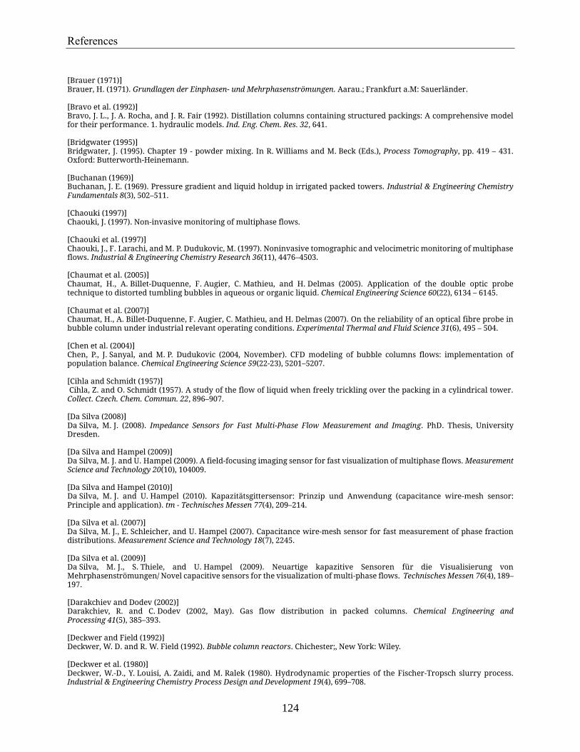
References
124
[Brauer (1971)] Brauer, H. (1971). Grundlagen der Einphasen- und Mehrphasenströmungen. Aarau.; Frankfurt a.M: Sauerländer. [Bravo et al. (1992)] Bravo, J. L., J. A. Rocha, and J. R. Fair (1992). Distillation columns containing structured packings: A comprehensive model for their performance. 1. hydraulic models. Ind. Eng. Chem. Res. 32, 641. [Bridgwater (1995)] Bridgwater, J. (1995). Chapter 19 - powder mixing. In R. Williams and M. Beck (Eds.), Process Tomography, pp. 419 – 431. Oxford: Butterworth-Heinemann. [Buchanan (1969)] Buchanan, J. E. (1969). Pressure gradient and liquid holdup in irrigated packed towers. Industrial & Engineering Chemistry Fundamentals 8(3), 502–511. [Chaouki (1997)] Chaouki, J. (1997). Non-invasive monitoring of multiphase flows. [Chaouki et al. (1997)] Chaouki, J., F. Larachi, and M. P. Dudukovic, M. (1997). Noninvasive tomographic and velocimetric monitoring of multiphase flows. Industrial & Engineering Chemistry Research 36(11), 4476–4503. [Chaumat et al. (2005)] Chaumat, H., A. Billet-Duquenne, F. Augier, C. Mathieu, and H. Delmas (2005). Application of the double optic probe technique to distorted tumbling bubbles in aqueous or organic liquid. Chemical Engineering Science 60(22), 6134 – 6145. [Chaumat et al. (2007)] Chaumat, H., A. Billet-Duquenne, F. Augier, C. Mathieu, and H. Delmas (2007). On the reliability of an optical fibre probe in bubble column under industrial relevant operating conditions. Experimental Thermal and Fluid Science 31(6), 495 – 504. [Chen et al. (2004)] Chen, P., J. Sanyal, and M. P. Dudukovic (2004, November). CFD modeling of bubble columns flows: implementation of population balance. Chemical Engineering Science 59(22-23), 5201–5207. [Cihla and Schmidt (1957)] Cihla, Z. and O. Schmidt (1957). A study of the flow of liquid when freely trickling over the packing in a cylindrical tower. Collect. Czech. Chem. Commun. 22, 896–907. [Da Silva (2008)] Da Silva, M. J. (2008). Impedance Sensors for Fast Multi-Phase Flow Measurement and Imaging. PhD. Thesis, University Dresden. [Da Silva and Hampel (2009)] Da Silva, M. J. and U. Hampel (2009). A field-focusing imaging sensor for fast visualization of multiphase flows. Measurement Science and Technology 20(10), 104009. [Da Silva and Hampel (2010)] Da Silva, M. J. and U. Hampel (2010). Kapazitätsgittersensor: Prinzip und Anwendung (capacitance wire-mesh sensor: Principle and application). tm - Technisches Messen 77(4), 209–214. [Da Silva et al. (2007)] Da Silva, M. J., E. Schleicher, and U. Hampel (2007). Capacitance wire-mesh sensor for fast measurement of phase fraction distributions. Measurement Science and Technology 18(7), 2245. [Da Silva et al. (2009)] Da Silva, M. J., S. Thiele, and U. Hampel (2009). Neuartige kapazitive Sensoren für die Visualisierung von Mehrphasenströmungen/ Novel capacitive sensors for the visualization of multi-phase flows. Technisches Messen 76(4), 189–197. [Darakchiev and Dodev (2002)] Darakchiev, R. and C. Dodev (2002, May). Gas flow distribution in packed columns. Chemical Engineering and Processing 41(5), 385–393. [Deckwer and Field (1992)] Deckwer, W. D. and R. W. Field (1992). Bubble column reactors. Chichester;, New York: Wiley. [Deckwer et al. (1980)] Deckwer, W.-D., Y. Louisi, A. Zaidi, and M. Ralek (1980). Hydrodynamic properties of the Fischer-Tropsch slurry process. Industrial & Engineering Chemistry Process Design and Development 19(4), 699–708.

References
125
[Delnoij et al. (1999)] Delnoij, E., J. Westerweel, N. Deen, J. Kuipers, and W. van Swaaij (1999). Ensemble correlation {PIV} applied to bubble plumes rising in a bubble column. Chemical Engineering Science 54(21), 5159 – 5171. [Dudlik et al. (2002)] Dudlik, A., S. Schönfeld, S. Schlüter, H. Fahlenkamp, and H.-M. Prasser (2002). Prevention of water hammer and cavitational hammer in pipeline systems. Chemical Engineering & Technology 25(9), 888–890. [Dudukovic (2002)] Dudukovic, M. P. (2002, August). Opaque multiphase flows: experiments and modeling. Experimental Thermal and Fluid Science 26(6-7), 747–761. [Dutkai and Ruckenstein (1968)] Dutkai, E. and E. Ruckenstein (1968). Liquid distribution in packed columns. Chemical Engineering Science 23(11), 1365 – 1373. [Dyakowski (1996)] Dyakowski, T. (1996). Process tomography applied to multi-phase flow measurement. Measurement Science and Technology 7(3), 343. [Euzen, Jp. et al. (2000)] Euzen, Jp., Krishna, R., and Gauthier, T. (2000). A scale-up strategy for a commercial scale bubble column slurry reactor for Fischer-Tropsch synthesis. Oil & Gas Science and Technology - Rev. IFP 55(4), 359–393. [Farid and Gunn (1978)] Farid, M. M. and D. J. Gunn (1978). Liquid distribution and redistribution in packed columns–ii. Experimental. Chemical Engineering Science 33(9), 1221–1231. [Fordham et al. (1999)] Fordham, E. J., A. Holmes, R. T. Ramos, S. Simonian, S.-M. Huang, and C. P. Lenn (1999). Multi-phase-fluid discrimination with local fibre-optical probes: I. liquid/liquid flows. Measurement Science and Technology 10(12), 1329. [Fordham et al. (1999)] Fordham, E. J., S. Simonian, R. T. Ramos, A. Holmes, S.-M. Huang, and C. P. Lenn (1999). Multi-phase-fluid discrimination with local fibre-optical probes: Ii. gas/liquid flows. Measurement Science and Technology 10(12), 1338. [Gross (1990)] Gross, R. (1990). Laser Doppler Anemometry Measurements in a Laboratory Model Bubble Column. West Virginia University. [Guet et al. (2005)] Guet, S., S. Luther, and G. Ooms (2005). Bubble shape and orientation determination with a four-point optical fibre probe. Experimental Thermal and Fluid Science 29(7), 803 – 812. [Gunn (1978)] Gunn, D. J. (1978). Liquid distribution and redistribution in packed columns-i theoretical. Chemical Engineering Science 33(9), 1211–1219. [Gunn and Al-Saffar (1993)] Gunn, D. J. and H. B. S. Al-Saffar (1993). Liquid distribution in packed columns. Chemical Engineering Science 48(22), 3845–3854. [Halow (1997)] Halow, J. (1997). Chapter 9 - electrical capacitance imaging of fluidized beds. In J. C. L. P. Dudukovic (Ed.), Non-Invasive Monitoring of Multiphase Flows, pp. 263 – 307. Amsterdam: Elsevier Science B.V. [Henley and Seader (1981)] Henley, E. J. and J. D. Seader (1981). Equilibrium Stage Separation Operations in Chemical Engineering. Wiley. Equilibrium Stage Separation. [Higler et al. (1999a)] Higler, A., R. Krishna, and R. Taylor (1999a). Nonequilibrium cell model for multicomponent (reactive) separation processes. AIChE Journal 45(11), 23572370. [Higler et al. (1999b)] Higler, A., R. Krishna, and R. Taylor (1999b, October). Nonequilibrium cell model for packed distillation columns - the influence of maldistribution. Industrial & Engineering Chemistry Research 38(10), 3988–3999. [Hoek et al. (1986)] Hoek, P. J., J. A. Wesselingh, and F. J. Zuiderweg (1986). Small scale and large scale liquid maldistribution in packed columns. Chem. Eng. Res. Des. 64, 431.

References
126
[Iliuta et al. (2004)] Iliuta, I., C. Petre, and F. Larachi (2004, February). Hydrodynamic continuum model for two-phase flow structured-packing-containing columns. Chemical Engineering Science 59(4), 879–888. [Ji (2007)] Ji, A. (2007). Analyse diskreter Flüssigkeits-Gasströmungen mit optischen Fasersensoren. PhD. Thesis, TU Dortmund. [Johnson (1987)] Johnson, I. (1987, Februar). Method and apparatus for measuring water in crude oil. US Patent 4,644,263. [Kiambi et al. (2001)] Kiambi, S., A. Duquenne, A. Bascoul, and H. Delmas (2001). Measurements of local interfacial area: application of bi-optical fibre technique. Chemical Engineering Science 56, 6447 – 6453. [Kipphan (1977)] Kipphan, H. (1977). Bestimmung von Transportkenngrößen bei Mehrphasenströmungen mit Hilfe der Korrelationsmesstechnik. Chemie Ingenieur Technik 49(9), 695–707. [Kouri and Sohlo (1996)] Kouri, R. and J. Sohlo (1996). Liquid and gas flow patterns in random packings. The Chemical Engineering Journal and the Biochemical Engineering Journal 61(2), 95 – 105. [Krishna et al. (1996)] Krishna, R., J. Ellenberger, and S. Sie (1996). Reactor development for conversion of natural gas to liquid fuels: A scale-up strategy relying on hydrodynamic analogies. Chemical Engineering Science 51(10), 2041 – 2050. Chemical Reaction Engineering: From Fundamentals to Commercial Plants and Products. [Kulkarni (2005)] Kulkarni, A. (2005). Effect of sparger design on the local flow field in a bubble column: Analysis using {LDA}. Chemical Engineering Research and Design 83(1), 59 – 66. [Loser (2002)] Loser, T. (2002). Berechnung der zweiphasigen Strömung in Schichtungen. Ph. D. thesis, University Hannover. [Loser et al. (2001)] Loser, T., R. Wajman, and D. Mewes (2001). Electrical capacitance tomography: image reconstruction along electric field lines. Measurement Science and Technology 12(8), 1083. [Luo et al. (1999)] Luo, X., D. J. Lee, R. Lau, G. Yang, and L.-S. Fan (1999). Maximum stable bubble size and gas holdup in high-pressure slurry bubble columns. AIChE Journal 45(4), 665–680. [Mackowiak (2010)] Mackowiak, J. (2010). Fluid Dynamics of Packed Columns. Springer. [Mahr and Mewes (2008)] Mahr, B. and D. Mewes (2008). Two-phase flow in structured packings: Modeling and calculation on a macroscopic scale. AIChE J. 54(3), 614–626. [Matusiak et al. (2010)] Matusiak, B., M. J. da Silva, U. Hampel, and A. Romanowski (2010). Measurement of dynamic liquid distributions in a fixed bed using electrical capacitance tomography and capacitance wire-mesh sensor. Ind. Eng. Chem. Res. 49(5), 2070–2077. [Mersmann and Deixler (1986)] Mersmann, A. and A. Deixler (1986). Packed columns. Ger. Chem. Eng. 9, 265. [Mewes and Fellhölter (1995)] Mewes, D. and A. Fellhölter (1995). Chapter 22 - mixing processes in fluids. In R. Williams and M. Beck (Eds.), Process Tomography, pp. 487 – 508. Oxford: Butterworth-Heinemann. [Miller and Mitchie (1970)] Miller, N. and R. Mitchie (1970). Measurement of local voidage in liquid/gas 2-phase flow systems using a universal probe. Journal of the british nuclear energy society 2(2), 94–100. [Mizushima et al. (2013)] Mizushima, Y., A. Sakamoto, and T. Saito (2013). Measurement technique of bubble velocity and diameter in a bubble column via single-tip optical-fiber probing with judgment of the pierced position and angle. Chemical Engineering Science 100(0), 98 – 104. 11th International Conference on Gas-Liquid and Gas-Liquid-Solid Reactor Engineering. [Olujic and de Graauw (1990)] Olujic, Z. and J. de Graauw (1990). Experimental studies on the interaction between the initial liquid distribution and the

References
127
performance of structured packings. Separation Science and Technology 25(13), 1723–1735. [Onda et al. (1968)] Onda, K., H. Takeuchi, and Y. Okumoto (1968). Mass transfer coefficients between gas and liquid phases in packed columns. J. Chem. Eng. Jpn. 1, 56. [Pakzad et al. (2008)] Pakzad, L., F. Ein-Mozaffari, and P. Chan (2008). Using electrical resistance tomography and computational fluid dynamics modeling to study the formation of cavern in the mixing of pseudoplastic fluids possessing yield stress. Chemical Engineering Science 63(9), 2508 – 2522. [Petrova et al. (2003)] Petrova, T., K. Semkov, and C. Dodev (2003, November). Mathematical modeling of gas distribution in packed columns. Chemical Engineering and Processing 42(11), 931–937. [Pizzo et al. (1998)] Pizzo, S. M., D. Moraes, F. A. N. Fernandes, M. S. Kobayasi, and R. J. Pazini (1998). Analysis of liquid distribution in a packed column on a pilot scale. Industrial & Engineering Chemistry Research 37(7), 2844–2849. [Polydorides and Lionheart (2002)] Polydorides, N. and W. R. B. Lionheart (2002). A matlab toolkit for three-dimensional electrical impedance tomography: a contribution to the electrical impedance and diffuse optical reconstruction software project. Measurement Science and Technology 13(12), 1871. [Potthoff (1992)] Potthoff, R. (1992). Maldistribution in Füllkörperkolonnen. Fortschritt-berichte VDI Reihe 3 Nr. 294. Düsseldorf: VDI-Verlag, University Essen. [Prasser (2008)] Prasser, H. M. (2008, March). Novel experimental measuring techniques required to provide data for CFD validation. Nuclear Engineering and Design 238(3), 744–770. [Prasser et al. (1998)] Prasser, H. M., A. Böttger, and J. Zschau (1998, June). A new electrode-mesh tomograph for gas-liquid flows. Flow Measurement and Instrumentation 9(2), 111–119. [Prasser et al. (2002)] Prasser, H. M., E. Krepper, and D. Lucas (2002, January). Evolution of the two-phase flow in a vertical tube–decomposition of gas fraction profiles according to bubble size classes using wire-mesh sensors. International Journal of Thermal Sciences 41(1), 17–28. [Prasser et al. (2003)] Prasser, H. M., D. Lucas, E. Krepper, and D. Baldauf (2003). Flow maps and models for transient two-phase flows. Technical Report 150 1215, Rossendorf-Institut. Report - No.: FZR-379. [Prasser et al. (2007)] Prasser, H. M., M. Misawa, and I. Tiseanu (2007, April). Comparison between wire-mesh sensor and ultra-fast x-ray tomograph for an air-water flow in a vertical pipe. Flow Measurement and Instrumentation 16(2-3), 73–83. [Reinecke et al. (1996)] Reinecke, N., M. Boddem, G. Petritsch, and D. Mewes (1996). Tomographisches Messen der relativen Phasenanteile in zweiphasigen Strömungen fluider Phasen. Chemie Ingenieur Technik 68(11), 1404–1412. [Rodriguez et al. (2014)] Rodriguez, I., H. V. Pena, A. B. Riano, R. Henkes, and O. Rodriguez (2014). Experiments with a wire-mesh sensor for stratified and dispersed oil-brine pipe flow. International Journal of Multiphase Flow 70(0), 113–125. [Rüdisüli et al. (2012)] Rüdisüli, M., T. J. Schildhauer, S. M. Biollaz, and J. R. van Ommen (2012). Bubble characterization in a fluidized bed by means of optical probes. International Journal of Multiphase Flow 41(0), 56 – 67. [Saberi et al. (1995)] Saberi, S., K. Shakourzadeh, D. Bastoul, and J. Militzer (1995). Bubble size and velocity measurement in gas-liquid systems: Application of fiber optic technique to pilot plant scale. The Canadian Journal of Chemical Engineering 73(2), 253–257. [Schubert et al. (2010)] Schubert, M., A. Khetan, M. J. da Silva, and H. Kryk (2010, April). Spatially resolved inline measurement of liquid velocity in trickle bed reactors. Chemical Engineering Science 158(3), 623–632. [Schubert et al. (2010)] Schubert, M., H. Kryk, and U. Hampel (2010). Slow-mode gas/liquid-induced periodic hydrodynamics in trickling packed beds derived from direct measurement of cross-sectional distributed local capacitances. Chemical Engineering and Processing:

References
128
Process Intensification 49(10), 1107–1121. [Sharaf et al. (2011)] Sharaf, S., M. Da Silva, U. Hampel, C. Zippe, M. Beyer, and B. Azzopardi (2011). Comparison between wire mesh sensor and gamma densitometry void measurements in two-phase flows. Measurement Science and Technology 22(10), 104019. [SHEW et al. (2006)] SHEW, W. L., S. PONCET, and J.-F. PINTON (2006, 11). Force measurements on rising bubbles. Journal of Fluid Mechanics 569, 51–60. [Stichlmair et al. (1989)] Stichlmair, J., J. L. Bravo, and J. R. Fair (1989, March). General model for prediction of pressure drop and capacity of countercurrent gas/liquid packed columns. Gas Separation & Purification 3(1), 19–28. [Stikkelman (1989)] Stikkelman, R. (1989). Gas and liquid maldistribution in packed columns. Ph. D. thesis, Delft University of Technology. [Stikkelman et al. (1989)] Stikkelman, R., H. Teeuw, H. Wesselingh, J. de Graauw, and Z. Olujic (1989). A study of gas and liquid distributions in structured packings. Chemical Engineering & Technology 12(1), 445–449. [Stoter et al. (1993)] Stoter, F., Z. Olujic, and J. Graauw (1993). Modelling and measurement of gas flow distribution in corrugated sheet structured packings. The Chemical Engineering Journal and the Biochemical Engineering Journal 53(1), 55–66. [Sun et al. (2000)] Sun, C., F. Yin, A. Afacan, K. Nandakumar, and K. Chuang (2000, April). Modelling and simulation of flow maldistribution in random packed columns with gas-liquid countercurrent flow. Chemical Engineering Research and Design 78(3), 378–388. [Therning and Rasmuson (2005)] Therning, P. and A. Rasmuson (2005). Lda measurements of liquid velocities in a refractive index matched packed bubble column. Chemical Engineering Science 60(3), 717 – 726. [Tour and Lerman (1939)] Tour, R. and F. Lerman (1939). An improved device to demonstrate the laws of frequency distribution. Transactions of the AIChE 35, 709–718. [Toye et al. (1996)] Toye, D., P. Marchot, M. Crine, and G. L’Homme (1996). Modelling of multiphase flow in packed beds by computer-assisted x-ray tomography. Measurement Science and Technology 7(3), 436. [Toye et al. (1997)] Toye, D., P. Marchot, M. Crine, and G. L’Homme (1997). Chapter 3 - computer-assisted tomography for liquid imaging in trickle flow columns. In J. C. L. P. Dudukovic (Ed.), Non-Invasive Monitoring of Multiphase Flows, pp. 105 – 139. Amsterdam: Elsevier Science B.V. [Vejrazka et al. (2010)] Vejrazka, J., M. Vecer, S. Orvalho, P. Sechet, M. C. Ruzicka, and A. Cartellier (2010). Measurement accuracy of a mono-fiber optical probe in a bubbly flow. International Journal of Multiphase Flow 36(7), 533 – 548. [Wallis (1969)] Wallis, G. B. (1969). One-dimensional two-phase flow. New York : McGraw-Hill. Includes bibliographical references. [Wang et al. (2000)] Wang, M., A. Dorward, D. Vlaev, and R. Mann (2000). Measurements of gas-liquid mixing in a stirred vessel using electrical resistance tomography (ert). Chemical Engineering Journal 77(1-2), 93 – 98. [Williams and Beck (1995)] Williams, R. and M. Beck (1995). Chapter 1 - introduction to process tomography. In R. Williams and M. Beck (Eds.), Process Tomography, pp. 3 – 12. Oxford: Butterworth-Heinemann. [Xie (1995)] Xie, C. (1995). Chapter 15 - image reconstruction. In R. Williams and M. Beck (Eds.), Process Tomography, pp. 281 – 323. Oxford: Butterworth-Heinemann. [Xue et al. (2008)] Xue, J., M. Al-Dahhan, M. P. Dudukovic, and R. F. Mudde (2008). Bubble velocity, size, and interfacial area measurements in a bubble column by four-point optical probe. AIChE Journal 54(2), 350–363. [Yin et al. (2002)] Yin, F., A. Afacan, K. Nandakumar, and K. T. Chuang (2002, May). Liquid holdup distribution in packed columns: gamma ray tomography and cfd simulation. Chemical Engineering and Processing 41(5), 473–483.

References
129
[Yin et al. (2000)] Yin, F., Z. C. Wang, A. Afacan, K. Nandakumar, and K. T. Chuang (2000). Experimental studies of liquid flow maldistribution in a random packed column. Can. J. Chem. Eng. 78(3), 449–457. [York (2001)] York, T. (2001). Status of electrical tomography in industrial applications. Journal of Electronic Imaging 10(3), 608. [Zhang et al. (2013)] Zhang, Z., M. Bieberle, F. Barthel, L. Szalinski, and U. Hampel (2013). Investigation of upward cocurrent gas-liquid pipe flow using ultrafast x-ray tomography and wire-mesh sensor. Flow Measurement and Instrumentation 32(0), 111 – 118. [Zuiderweg et al. (1993)] Zuiderweg, F. J., J. G. Kunesh, and D. W. King (1993). A model for the calculation of the effect of maldistribution on the efficiency of a packed column. Trans. IChemE 71, 38.
Lebenslauf und Bildungsgang
01/2016 Evonik Technology & Infrastructure GmbH Chemiepark Marl Prozesssicherheit Ingenieur für Prozesssicherheit
11/2014 -12/2015 Evonik Technology & Infrastructure GmbH Chemiepark Marl Technische Anlagensicherheit Ingenieur für Anlagensicherheit
11/2013 -10/2014 Excellence AG Ingenieur für Anlagensicherheit
01/2009 - 07/2013 Promotion im Bereich Fluidverfahrenstechnik an der Ruhr-Universität Bochum
10/2003 - 11/2008 Diplomstudium Bio- und Chemieingenieurwesen an der Technischen Universität Dortmund Abschluss: Diplomingenieur
09/2002 - 09/2003 Sprachkurs (Deutsch) in Berlin
09/1999 - 07/2002 Technische Universität Harbin, China
09/1996 - 07/1999 Oberschule in Jilin, China
09/1993 - 07/1996 Mittelschule in Jilin, China
09/1987 – 07/1993 Grundschule in Jilin, China
14.02.1980 Geburt in Jilin, China