STUDY MATERIAL FOR B.SC CS COMPUTER GRAPHICS AND ...
72
STUDY MATERIAL FOR B.SC CS COMPUTER GRAPHICS AND VISUALIZATION SEMESTER - VI, ACADEMIC YEAR 2020 - 21 Page 1 of 72 UNIT CONTENT PAGE Nr I OVERVIEW OF GRAPHICS SYSTEM 02 II ATTRIBUTES OF OUTPUT PRIMITIVES 30 III TWO DIMENSIONAL VIEWING 45 IV GRAPHICAL USER INTERFACES AND INTERACTIVE 54 V THREE-DIMENSIONAL VIEWING 62
Transcript of STUDY MATERIAL FOR B.SC CS COMPUTER GRAPHICS AND ...
STUDY MATERIAL FOR B.SC CS COMPUTER GRAPHICS AND VISUALIZATION SEMESTER - VI, ACADEMIC YEAR 2020 - 21
Page 1 of 72
UNIT CONTENT PAGE Nr
I OVERVIEW OF GRAPHICS SYSTEM 02
II ATTRIBUTES OF OUTPUT PRIMITIVES 30
III TWO DIMENSIONAL VIEWING 45
IV GRAPHICAL USER INTERFACES AND INTERACTIVE 54
V THREE-DIMENSIONAL VIEWING 62
STUDY MATERIAL FOR B.SC CS COMPUTER GRAPHICS AND VISUALIZATION SEMESTER - VI, ACADEMIC YEAR 2020 - 21
Page 2 of 72
UNIT - I OVERVIEW OF GRAPHICS SYSTEM
Visual Display Devices:
The primary output device in a graphics system is a video monitor. Although many technologies exist, but the operation of most video monitors is based on the standard Cathode Ray Tube (CRT) design. Cathode Ray Tubes (CRT):
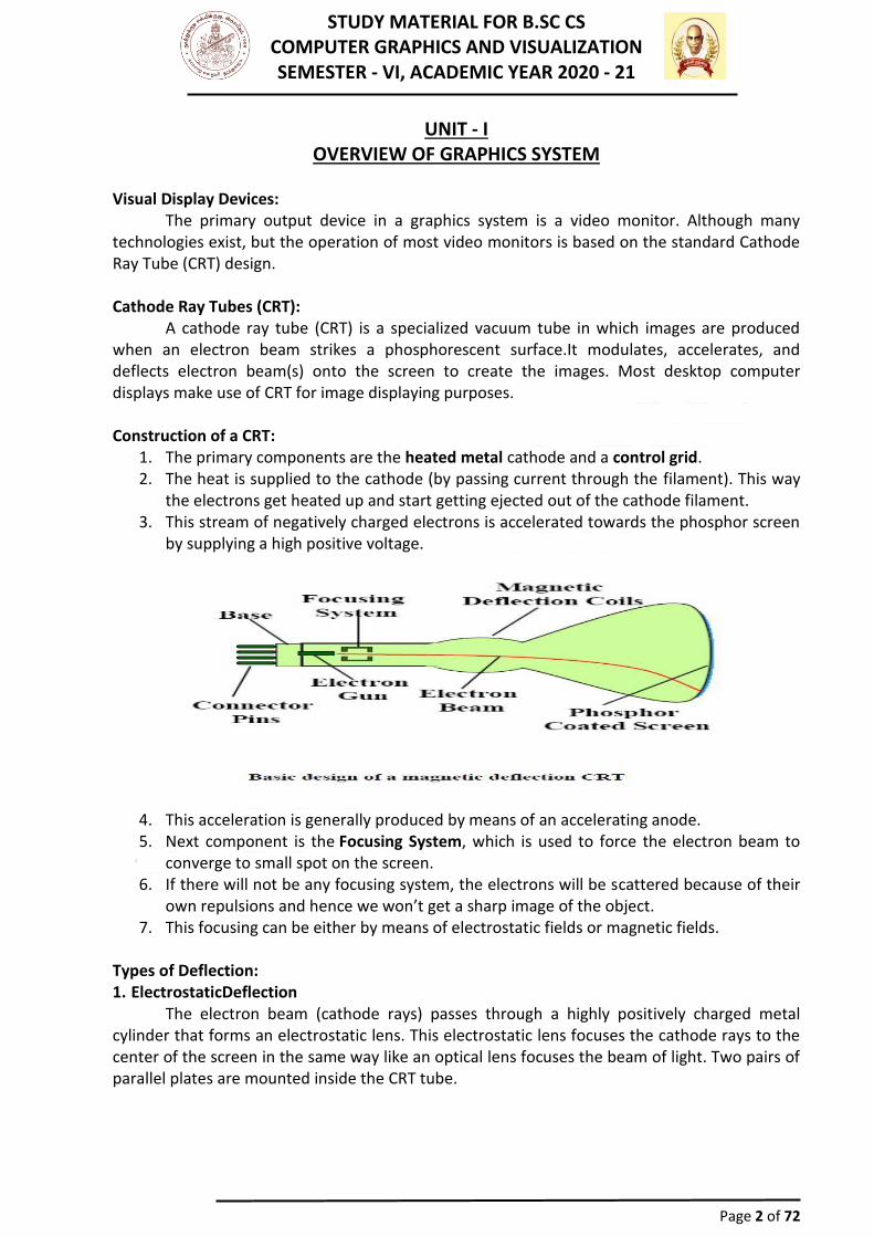
A cathode ray tube (CRT) is a specialized vacuum tube in which images are produced when an electron beam strikes a phosphorescent surface.It modulates, accelerates, and deflects electron beam(s) onto the screen to create the images. Most desktop computer displays make use of CRT for image displaying purposes. Construction of a CRT:
1. The primary components are the heated metal cathode and a control grid. 2. The heat is supplied to the cathode (by passing current through the filament). This way
the electrons get heated up and start getting ejected out of the cathode filament. 3. This stream of negatively charged electrons is accelerated towards the phosphor screen
by supplying a high positive voltage.
4. This acceleration is generally produced by means of an accelerating anode. 5. Next component is the Focusing System, which is used to force the electron beam to
converge to small spot on the screen. 6. If there will not be any focusing system, the electrons will be scattered because of their
own repulsions and hence we won’t get a sharp image of the object. 7. This focusing can be either by means of electrostatic fields or magnetic fields.
Types of Deflection: 1. ElectrostaticDeflection
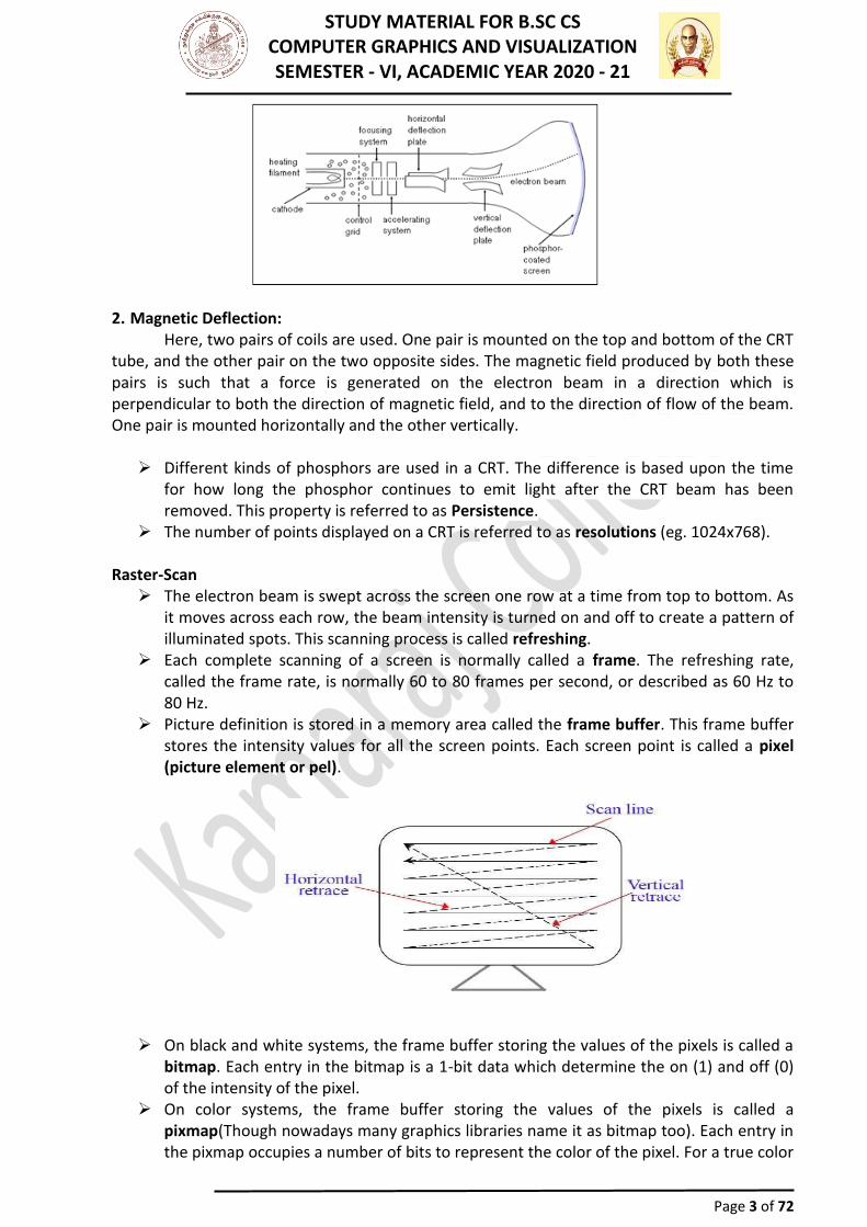
The electron beam (cathode rays) passes through a highly positively charged metal cylinder that forms an electrostatic lens. This electrostatic lens focuses the cathode rays to the center of the screen in the same way like an optical lens focuses the beam of light. Two pairs of parallel plates are mounted inside the CRT tube.
STUDY MATERIAL FOR B.SC CS COMPUTER GRAPHICS AND VISUALIZATION SEMESTER - VI, ACADEMIC YEAR 2020 - 21
Page 3 of 72
2. Magnetic Deflection:
Here, two pairs of coils are used. One pair is mounted on the top and bottom of the CRT tube, and the other pair on the two opposite sides. The magnetic field produced by both these pairs is such that a force is generated on the electron beam in a direction which is perpendicular to both the direction of magnetic field, and to the direction of flow of the beam. One pair is mounted horizontally and the other vertically.
➢ Different kinds of phosphors are used in a CRT. The difference is based upon the time for how long the phosphor continues to emit light after the CRT beam has been removed. This property is referred to as Persistence.
➢ The number of points displayed on a CRT is referred to as resolutions (eg. 1024x768). Raster-Scan
➢ The electron beam is swept across the screen one row at a time from top to bottom. As it moves across each row, the beam intensity is turned on and off to create a pattern of illuminated spots. This scanning process is called refreshing.
➢ Each complete scanning of a screen is normally called a frame. The refreshing rate, called the frame rate, is normally 60 to 80 frames per second, or described as 60 Hz to 80 Hz.
➢ Picture definition is stored in a memory area called the frame buffer. This frame buffer stores the intensity values for all the screen points. Each screen point is called a pixel (picture element or pel).
➢ On black and white systems, the frame buffer storing the values of the pixels is called a
bitmap. Each entry in the bitmap is a 1-bit data which determine the on (1) and off (0) of the intensity of the pixel.
➢ On color systems, the frame buffer storing the values of the pixels is called a pixmap(Though nowadays many graphics libraries name it as bitmap too). Each entry in the pixmap occupies a number of bits to represent the color of the pixel. For a true color
STUDY MATERIAL FOR B.SC CS COMPUTER GRAPHICS AND VISUALIZATION SEMESTER - VI, ACADEMIC YEAR 2020 - 21
Page 4 of 72
display, the number of bits for each entry is 24 (8 bits per red/green/blue channel, each channel 28 =256 levels of intensity value, ie. 256 voltage settings for each of the red/green/blue electron guns).
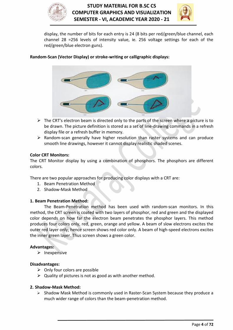
Random-Scan (Vector Display) or stroke-writing or calligraphic displays:
➢ The CRT's electron beam is directed only to the parts of the screen where a picture is to
be drawn. The picture definition is stored as a set of line-drawing commands in a refresh display file or a refresh buffer in memory.
➢ Random-scan generally have higher resolution than raster systems and can produce smooth line drawings, however it cannot display realistic shaded scenes.
Color CRT Monitors: The CRT Monitor display by using a combination of phosphors. The phosphors are different colors. There are two popular approaches for producing color displays with a CRT are:
1. Beam Penetration Method 2. Shadow-Mask Method
1. Beam Penetration Method:
The Beam-Penetration method has been used with random-scan monitors. In this method, the CRT screen is coated with two layers of phosphor, red and green and the displayed color depends on how far the electron beam penetrates the phosphor layers. This method produces four colors only, red, green, orange and yellow. A beam of slow electrons excites the outer red layer only; hence screen shows red color only. A beam of high-speed electrons excites the inner green layer. Thus screen shows a green color. Advantages:
➢ Inexpensive Disadvantages:
➢ Only four colors are possible ➢ Quality of pictures is not as good as with another method.
2. Shadow-Mask Method:
➢ Shadow Mask Method is commonly used in Raster-Scan System because they produce a much wider range of colors than the beam-penetration method.
STUDY MATERIAL FOR B.SC CS COMPUTER GRAPHICS AND VISUALIZATION SEMESTER - VI, ACADEMIC YEAR 2020 - 21
Page 5 of 72
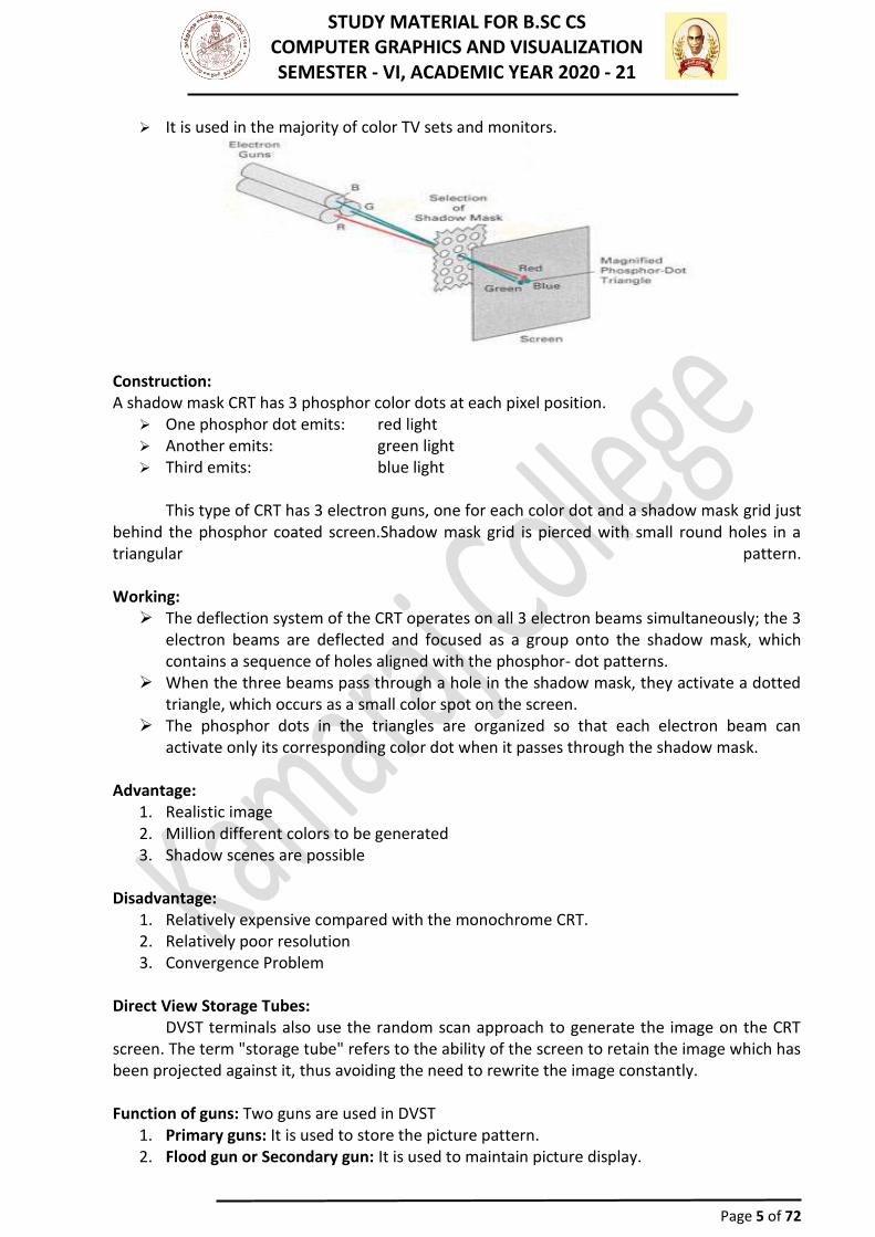
➢ It is used in the majority of color TV sets and monitors.
Construction: A shadow mask CRT has 3 phosphor color dots at each pixel position.
➢ One phosphor dot emits: red light ➢ Another emits: green light ➢ Third emits: blue light
This type of CRT has 3 electron guns, one for each color dot and a shadow mask grid just
behind the phosphor coated screen.Shadow mask grid is pierced with small round holes in a triangular pattern. Working:
➢ The deflection system of the CRT operates on all 3 electron beams simultaneously; the 3 electron beams are deflected and focused as a group onto the shadow mask, which contains a sequence of holes aligned with the phosphor- dot patterns.
➢ When the three beams pass through a hole in the shadow mask, they activate a dotted triangle, which occurs as a small color spot on the screen.
➢ The phosphor dots in the triangles are organized so that each electron beam can activate only its corresponding color dot when it passes through the shadow mask.
Advantage:
1. Realistic image 2. Million different colors to be generated 3. Shadow scenes are possible
Disadvantage:
1. Relatively expensive compared with the monochrome CRT. 2. Relatively poor resolution 3. Convergence Problem
Direct View Storage Tubes:
DVST terminals also use the random scan approach to generate the image on the CRT screen. The term "storage tube" refers to the ability of the screen to retain the image which has been projected against it, thus avoiding the need to rewrite the image constantly. Function of guns: Two guns are used in DVST
1. Primary guns: It is used to store the picture pattern. 2. Flood gun or Secondary gun: It is used to maintain picture display.
STUDY MATERIAL FOR B.SC CS COMPUTER GRAPHICS AND VISUALIZATION SEMESTER - VI, ACADEMIC YEAR 2020 - 21
Page 6 of 72
Advantage: 1. No refreshing is needed. 2. High Resolution 3. Cost is very less
Disadvantage:
1. It is not possible to erase the selected part of a picture. 2. It is not suitable for dynamic graphics applications. 3. If a part of picture is to modify, then time is consumed.
Flat Panel Display:
The Flat-Panel display refers to a class of video devices that have reduced volume, weight and power requirement compare to CRT. Example: Small T.V. monitor, calculator, pocket video games, laptop computers, an advertisement board in elevator. 1. Emissive Display:
The emissive displays are devices that convert electrical energy into light. Examples are Plasma Panel, thin film electroluminescent display and LED (Light Emitting Diodes). 2. Non-Emissive Display:
The Non-Emissive displays use optical effects to convert sunlight or light from some other source into graphics patterns. Examples are LCD (Liquid Crystal Device). Plasma Panel Display:
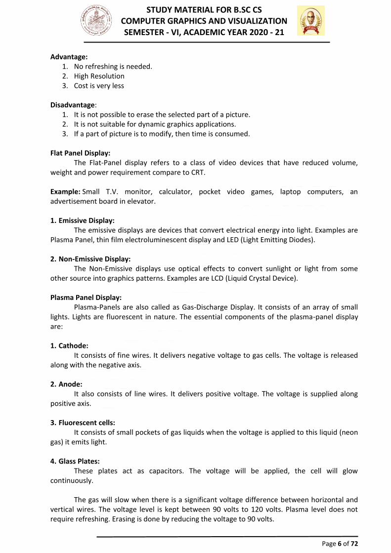
Plasma-Panels are also called as Gas-Discharge Display. It consists of an array of small lights. Lights are fluorescent in nature. The essential components of the plasma-panel display are: 1. Cathode:
It consists of fine wires. It delivers negative voltage to gas cells. The voltage is released along with the negative axis. 2. Anode:
It also consists of line wires. It delivers positive voltage. The voltage is supplied along positive axis. 3. Fluorescent cells:
It consists of small pockets of gas liquids when the voltage is applied to this liquid (neon gas) it emits light. 4. Glass Plates:
These plates act as capacitors. The voltage will be applied, the cell will glow continuously.
The gas will slow when there is a significant voltage difference between horizontal and vertical wires. The voltage level is kept between 90 volts to 120 volts. Plasma level does not require refreshing. Erasing is done by reducing the voltage to 90 volts.
STUDY MATERIAL FOR B.SC CS COMPUTER GRAPHICS AND VISUALIZATION SEMESTER - VI, ACADEMIC YEAR 2020 - 21
Page 7 of 72
Each cell of plasma has two states, so cell is said to be stable. Displayable point in plasma panel is made by the crossing of the horizontal and vertical grid. The resolution of the plasma panel can be up to 512 * 512 pixels. Advantage:
1. High Resolution 2. Large screen size is also possible. 3. Less Volume 4. Less weight 5. Flicker Free Display
Disadvantage:
1. Poor Resolution 2. Wiring requirement anode and the cathode is complex. 3. Its addressing is also complex.
LED (Light Emitting Diode):
➢ In an LED, a matrix of diodes is organized to form the pixel positions in the display and picture definition is stored in a refresh buffer. Data is read from the refresh buffer and converted to voltage levels that are applied to the diodes to produce the light pattern in the display.
LCD (Liquid Crystal Display): ➢ Liquid Crystal Displays are the devices that produce a picture by passing polarized light
from the surroundings or from an internal light source through a liquid-crystal material that transmits the light.
➢ LCD uses the liquid-crystal material between two glass plates; each plate is the right angle to each other between plates liquid is filled. One glass plate consists of rows of conductors arranged in vertical direction. Another glass plate is consisting of a row of conductors arranged in horizontal direction. The pixel position is determined by the intersection of the vertical & horizontal conductor. This position is an active part of the screen.
➢ Liquid crystal display is temperature dependent. It is between zero to seventy degree Celsius. It is flat and requires very little power to operate.
Advantage:
1. Low power consumption. 2. Small Size 3. Low Cost
Disadvantage:
1. LCDs are temperature-dependent (0-70°C) 2. LCDs do not emit light; as a result, the image has very little contrast. 3. LCDs have no color capability. 4. The resolution is not as good as that of a CRT.
Input Devices
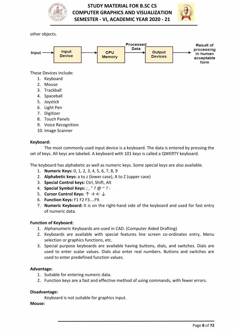
The Input Devices are the hardware that is used to transfer transfers input to the computer. The data can be in the form of text, graphics, sound, and text. Output device display data from the memory of the computer. Output can be text, numeric data, line, polygon, and
STUDY MATERIAL FOR B.SC CS COMPUTER GRAPHICS AND VISUALIZATION SEMESTER - VI, ACADEMIC YEAR 2020 - 21
Page 8 of 72
other objects.
These Devices include:
1. Keyboard 2. Mouse 3. Trackball 4. Spaceball 5. Joystick 6. Light Pen 7. Digitizer 8. Touch Panels 9. Voice Recognition 10. Image Scanner
Keyboard:
The most commonly used input device is a keyboard. The data is entered by pressing the set of keys. All keys are labeled. A keyboard with 101 keys is called a QWERTY keyboard. The keyboard has alphabetic as well as numeric keys. Some special keys are also available.
1. Numeric Keys: 0, 1, 2, 3, 4, 5, 6, 7, 8, 9 2. Alphabetic keys: a to z (lower case), A to Z (upper case) 3. Special Control keys: Ctrl, Shift, Alt 4. Special Symbol Keys: ; , " ? @ ~ ? : 5. Cursor Control Keys: ↑ → ← ↓ 6. Function Keys: F1 F2 F3....F9. 7. Numeric Keyboard: It is on the right-hand side of the keyboard and used for fast entry
of numeric data. Function of Keyboard:
1. Alphanumeric Keyboards are used in CAD. (Computer Aided Drafting) 2. Keyboards are available with special features line screen co-ordinates entry, Menu
selection or graphics functions, etc. 3. Special purpose keyboards are available having buttons, dials, and switches. Dials are
used to enter scalar values. Dials also enter real numbers. Buttons and switches are used to enter predefined function values.
Advantage:
1. Suitable for entering numeric data. 2. Function keys are a fast and effective method of using commands, with fewer errors.
Disadvantage:
Keyboard is not suitable for graphics input. Mouse:
STUDY MATERIAL FOR B.SC CS COMPUTER GRAPHICS AND VISUALIZATION SEMESTER - VI, ACADEMIC YEAR 2020 - 21
Page 9 of 72
A Mouse is a pointing device and used to position the pointer on the screen. It is a small
palm size box. There are two or three depression switches on the top. The movement of the mouse along the x-axis helps in the horizontal movement of the cursor and the movement along the y-axis helps in the vertical movement of the cursor on the screen. The mouse cannot be used to enter text. Therefore, they are used in conjunction with a keyboard. Advantage:
1. Easy to use 2. Not very expensive
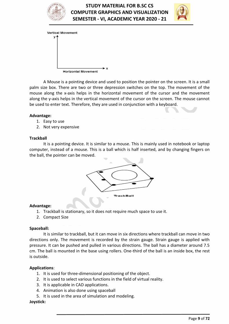
Trackball
It is a pointing device. It is similar to a mouse. This is mainly used in notebook or laptop computer, instead of a mouse. This is a ball which is half inserted, and by changing fingers on the ball, the pointer can be moved.
Advantage:
1. Trackball is stationary, so it does not require much space to use it. 2. Compact Size
Spaceball:
It is similar to trackball, but it can move in six directions where trackball can move in two directions only. The movement is recorded by the strain gauge. Strain gauge is applied with pressure. It can be pushed and pulled in various directions. The ball has a diameter around 7.5 cm. The ball is mounted in the base using rollers. One-third of the ball is an inside box, the rest is outside. Applications:
1. It is used for three-dimensional positioning of the object. 2. It is used to select various functions in the field of virtual reality. 3. It is applicable in CAD applications. 4. Animation is also done using spaceball 5. It is used in the area of simulation and modeling.
Joystick:
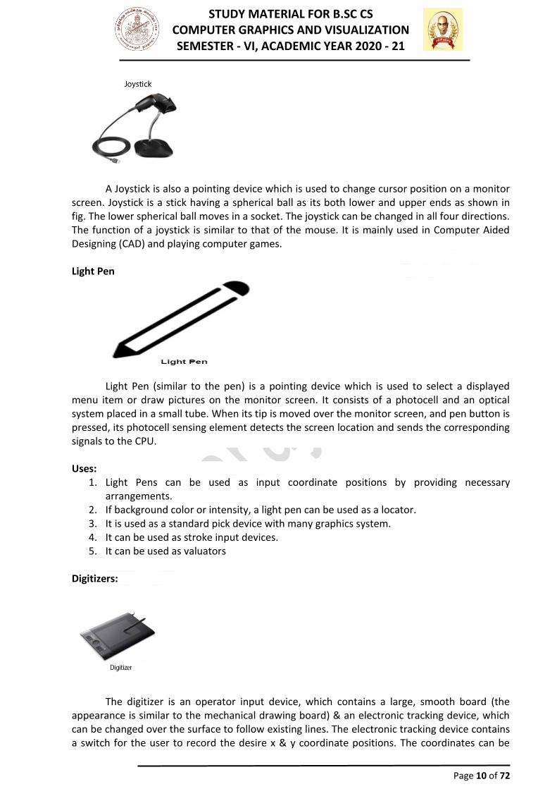
STUDY MATERIAL FOR B.SC CS COMPUTER GRAPHICS AND VISUALIZATION SEMESTER - VI, ACADEMIC YEAR 2020 - 21
Page 10 of 72
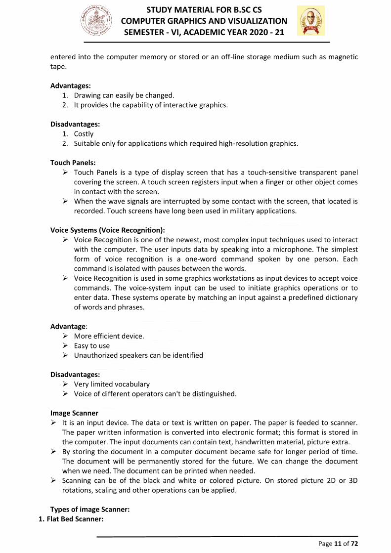
A Joystick is also a pointing device which is used to change cursor position on a monitor screen. Joystick is a stick having a spherical ball as its both lower and upper ends as shown in fig. The lower spherical ball moves in a socket. The joystick can be changed in all four directions. The function of a joystick is similar to that of the mouse. It is mainly used in Computer Aided Designing (CAD) and playing computer games. Light Pen
Light Pen (similar to the pen) is a pointing device which is used to select a displayed
menu item or draw pictures on the monitor screen. It consists of a photocell and an optical system placed in a small tube. When its tip is moved over the monitor screen, and pen button is pressed, its photocell sensing element detects the screen location and sends the corresponding signals to the CPU. Uses:
1. Light Pens can be used as input coordinate positions by providing necessary arrangements.
2. If background color or intensity, a light pen can be used as a locator. 3. It is used as a standard pick device with many graphics system. 4. It can be used as stroke input devices. 5. It can be used as valuators
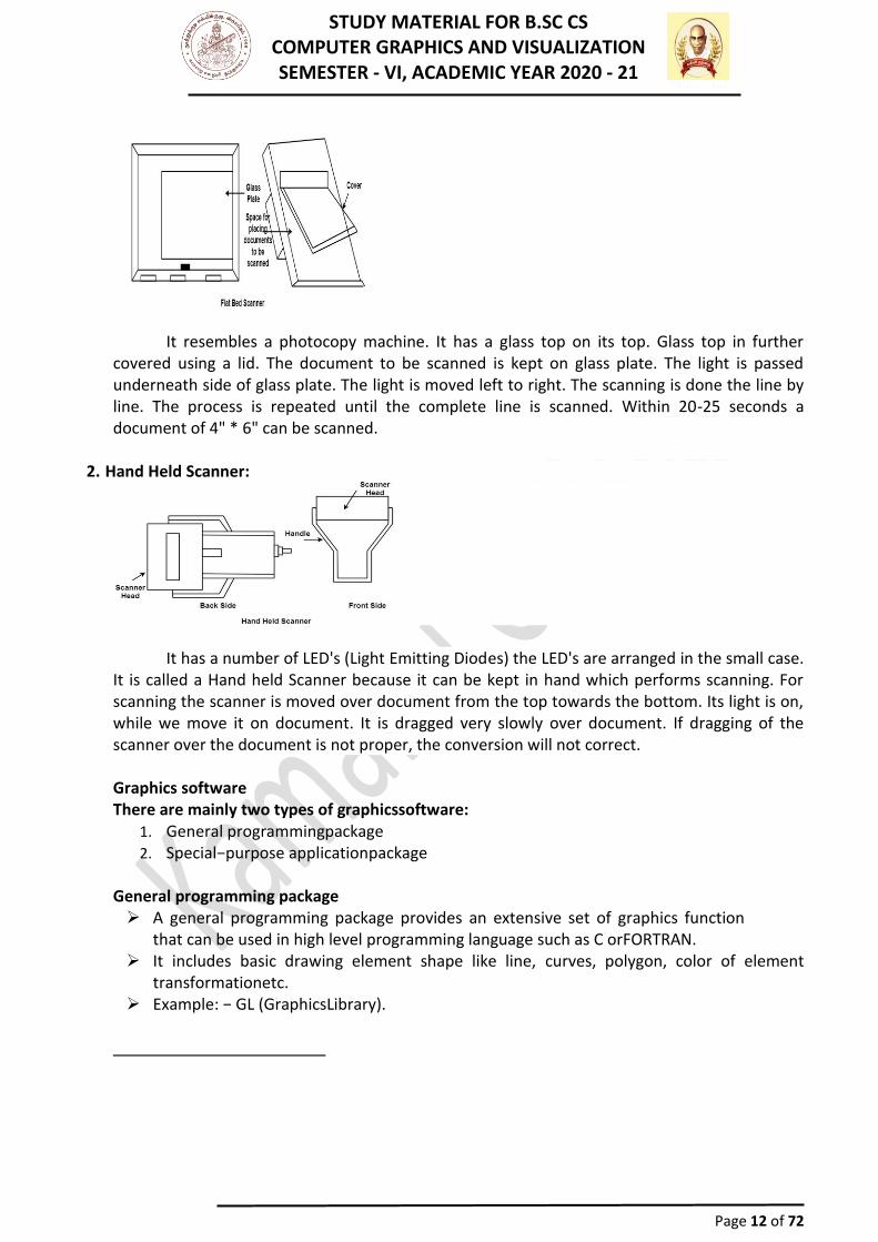
Digitizers:
The digitizer is an operator input device, which contains a large, smooth board (the appearance is similar to the mechanical drawing board) & an electronic tracking device, which can be changed over the surface to follow existing lines. The electronic tracking device contains a switch for the user to record the desire x & y coordinate positions. The coordinates can be
STUDY MATERIAL FOR B.SC CS COMPUTER GRAPHICS AND VISUALIZATION SEMESTER - VI, ACADEMIC YEAR 2020 - 21
Page 11 of 72
entered into the computer memory or stored or an off-line storage medium such as magnetic tape. Advantages:
1. Drawing can easily be changed. 2. It provides the capability of interactive graphics.
Disadvantages:
1. Costly 2. Suitable only for applications which required high-resolution graphics.
Touch Panels:
➢ Touch Panels is a type of display screen that has a touch-sensitive transparent panel covering the screen. A touch screen registers input when a finger or other object comes in contact with the screen.
➢ When the wave signals are interrupted by some contact with the screen, that located is recorded. Touch screens have long been used in military applications.
Voice Systems (Voice Recognition):
➢ Voice Recognition is one of the newest, most complex input techniques used to interact with the computer. The user inputs data by speaking into a microphone. The simplest form of voice recognition is a one-word command spoken by one person. Each command is isolated with pauses between the words.
➢ Voice Recognition is used in some graphics workstations as input devices to accept voice commands. The voice-system input can be used to initiate graphics operations or to enter data. These systems operate by matching an input against a predefined dictionary of words and phrases.
Advantage:
➢ More efficient device. ➢ Easy to use ➢ Unauthorized speakers can be identified
Disadvantages:
➢ Very limited vocabulary ➢ Voice of different operators can't be distinguished.
Image Scanner ➢ It is an input device. The data or text is written on paper. The paper is feeded to scanner.
The paper written information is converted into electronic format; this format is stored in the computer. The input documents can contain text, handwritten material, picture extra.
➢ By storing the document in a computer document became safe for longer period of time. The document will be permanently stored for the future. We can change the document when we need. The document can be printed when needed.
➢ Scanning can be of the black and white or colored picture. On stored picture 2D or 3D rotations, scaling and other operations can be applied.
Types of image Scanner:
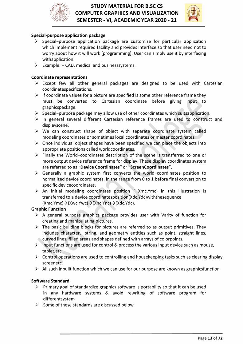
1. Flat Bed Scanner:
STUDY MATERIAL FOR B.SC CS COMPUTER GRAPHICS AND VISUALIZATION SEMESTER - VI, ACADEMIC YEAR 2020 - 21
Page 12 of 72
It resembles a photocopy machine. It has a glass top on its top. Glass top in further covered using a lid. The document to be scanned is kept on glass plate. The light is passed underneath side of glass plate. The light is moved left to right. The scanning is done the line by line. The process is repeated until the complete line is scanned. Within 20-25 seconds a document of 4" * 6" can be scanned.
2. Hand Held Scanner:
It has a number of LED's (Light Emitting Diodes) the LED's are arranged in the small case. It is called a Hand held Scanner because it can be kept in hand which performs scanning. For scanning the scanner is moved over document from the top towards the bottom. Its light is on, while we move it on document. It is dragged very slowly over document. If dragging of the scanner over the document is not proper, the conversion will not correct. Graphics software There are mainly two types of graphicssoftware:
1. General programmingpackage 2. Special−purpose applicationpackage
General programming package ➢ A general programming package provides an extensive set of graphics function
that can be used in high level programming language such as C orFORTRAN. ➢ It includes basic drawing element shape like line, curves, polygon, color of element
transformationetc. ➢ Example: − GL (GraphicsLibrary).
STUDY MATERIAL FOR B.SC CS COMPUTER GRAPHICS AND VISUALIZATION SEMESTER - VI, ACADEMIC YEAR 2020 - 21
Page 13 of 72
Special-purpose application package ➢ Special−purpose application package are customize for particular application
which implement required facility and provides interface so that user need not to worry about how it will work (programming). User can simply use it by interfacing withapplication.
➢ Example: − CAD, medical and businesssystems. Coordinate representations ➢ Except few all other general packages are designed to be used with Cartesian
coordinatespecifications. ➢ If coordinate values for a picture are specified is some other reference frame they
must be converted to Cartesian coordinate before giving input to graphicspackage.
➢ Special−purpose package may allow use of other coordinates which suitsapplication. ➢ In general several different Cartesian reference frames are used to construct and
displayscene. ➢ We can construct shape of object with separate coordinate system called
modeling coordinates or sometimes local coordinates or master coordinates. ➢ Once individual object shapes have been specified we can place the objects into
appropriate positions called worldcoordinates. ➢ Finally the World−coordinates description of the scene is transferred to one or
more output device reference frame for display. These display coordinates system are referred to as “Device Coordinates” or “ScreenCoordinates”.
➢ Generally a graphic system first converts the world−coordinates position to normalized device coordinates. In the range from 0 to 1 before final conversion to specific devicecoordinates.
➢ An initial modeling coordinates position ( Xmc,Ymc) in this illustration is transferred to a device coordinatesposition(Xdc,Ydc)withthesequence (Xmc,Ymc)→(Xwc,Ywc)→(Xnc,Ync)→(Xdc,Ydc).
Graphic Function ➢ A general purpose graphics package provides user with Varity of function for
creating and manipulating pictures. ➢ The basic building blocks for pictures are referred to as output primitives. They
includes character, string, and geometry entities such as point, straight lines, curved lines, filled areas and shapes defined with arrays of colorpoints.
➢ Input functions are used for control & process the various input device such as mouse, tablet,etc.
➢ Control operations are used to controlling and housekeeping tasks such as clearing display screenetc.
➢ All such inbuilt function which we can use for our purpose are known as graphicsfunction Software Standard ➢ Primary goal of standardize graphics software is portability so that it can be used
in any hardware systems & avoid rewriting of software program for differentsystem
➢ Some of these standards are discussed below
STUDY MATERIAL FOR B.SC CS COMPUTER GRAPHICS AND VISUALIZATION SEMESTER - VI, ACADEMIC YEAR 2020 - 21
Page 14 of 72
Graphical Kernel System (GKS) ➢ This system was adopted as a first graphics software standard by the
international standard organization (ISO) and various national standard organizations includingANSI.
➢ GKS was originally designed as the two dimensional graphics package and then later extension was developed for threedimensions.
PHIGS (Programmer’s Hierarchical Interactive Graphic Standard) ➢ PHIGS is extension of GKS. Increased capability for object modeling, color
specifications, surface rendering, and picture manipulation are provided inPHIGS. ➢ Extension of PHIGS called “PHIGS+” was developed to provide three dimensional
surface shading capabilities not available inPHIGS. OUTPUT PRIMITIVES Points and Lines ➢ Point plotting is done by converting a single coordinate position furnished by an
application program into appropriate operations for the output device inuse. ➢ Line drawing is done by calculating intermediate positions along the line path
between two specified endpointpositions. ➢ The output device is then directed to fill in those positions between the end
points with somecolor. ➢ For some device such as a pen plotter or random scan display, a straight line can
be drawn smoothly from one end point toother. ➢ Digital devices display a straight line segment by plotting discrete points between
the twoendpoints. ➢ Discrete coordinate positions along the line path are calculated from the
equation of theline. ➢ For a raster video display, the line intensity is loaded in frame buffer at the
corresponding pixel positions. ➢ Reading from the frame buffer, the video controller then plots the screenpixels. ➢ Screen locations are referenced with integer values, so plotted positions may only
approximate actual line positions between two specifiedendpoints. ➢ For example line position of (12.36, 23.87) would be converted to pixel position
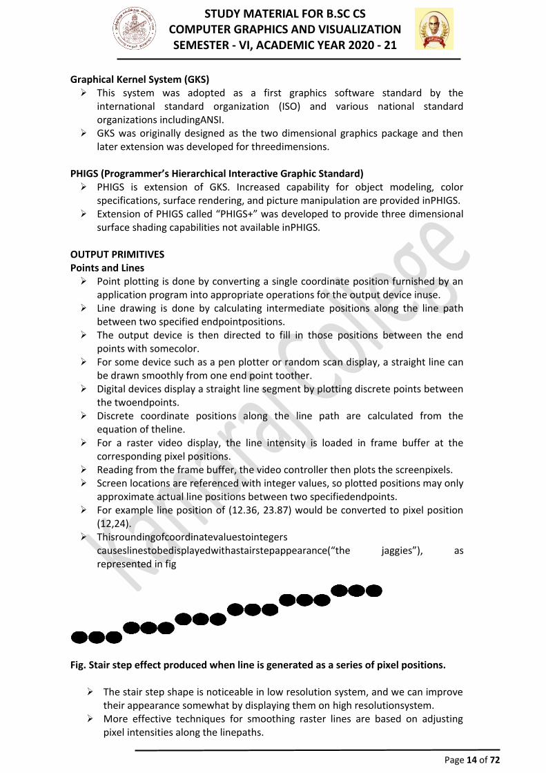
(12,24). ➢ Thisroundingofcoordinatevaluestointegers
causeslinestobedisplayedwithastairstepappearance(“the jaggies”), as represented in fig
Fig. Stair step effect produced when line is generated as a series of pixel positions.
➢ The stair step shape is noticeable in low resolution system, and we can improve their appearance somewhat by displaying them on high resolutionsystem.
➢ More effective techniques for smoothing raster lines are based on adjusting pixel intensities along the linepaths.
STUDY MATERIAL FOR B.SC CS COMPUTER GRAPHICS AND VISUALIZATION SEMESTER - VI, ACADEMIC YEAR 2020 - 21
Page 15 of 72
6
5
4
3
2
1
0
0 1 2 3 4 5 6
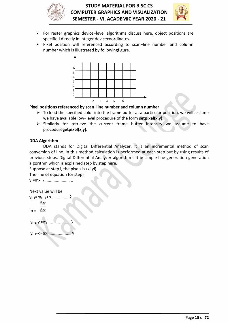
➢ For raster graphics device−level algorithms discuss here, object positions are specified directly in integer devicecoordinates.
➢ Pixel position will referenced according to scan−line number and column number which is illustrated by followingfigure.
Pixel positions referenced by scan−line number and column number ➢ To load the specified color into the frame buffer at a particular position, we will assume
we have available low−level procedure of the form setpixel(x,y). ➢ Similarly for retrieve the current frame buffer intensity we assume to have
proceduregetpixel(x,y). DDA Algorithm
DDA stands for Digital Differential Analyzer. It is an incremental method of scan conversion of line. In this method calculation is performed at each step but by using results of previous steps. Digital Differential Analyzer algorithm is the simple line generation generation algorithm which is explained step by step here. Suppose at step i, the pixels is (xi,yi) The line of equation for step i yi=mxi+b...................... 1 Next value will be yi+1=mxi+1+b............... 2
m = yi+1-yi=∆y................... 3 yi+1-xi=∆x.....................4
STUDY MATERIAL FOR B.SC CS COMPUTER GRAPHICS AND VISUALIZATION SEMESTER - VI, ACADEMIC YEAR 2020 - 21
Page 16 of 72
yi+1=yi+∆y ∆y=m∆x yi+1=yi+m∆x ∆x=∆y/m xi+1=xi+∆x xi+1=xi+∆y/m Case1: When |m|<1 then (assume that x1<x2)
x= x1,y=y1 set ∆x=1 yi+1=y1+m, x=x+1 Until x = x2 Case2: When |m|>1 then (assume that y1<y2) x= x1,y=y1 set ∆y=1
xi+1= , y=y+1 Until y → y2 Advantage:
1. It is a faster method than method of using direct use of line equation. 2. This method does not use multiplication theorem. 3. It allows us to detect the change in the value of x and y ,so plotting of same point twice
is not possible. 4. This method gives overflow indication when a point is repositioned. 5. It is an easy method because each step involves just two additions.
Disadvantage:
1. It involves floating point additions rounding off is done. Accumulations of round off error cause accumulation of error.
2. Rounding off operations and floating point operations consumes a lot of time.
STUDY MATERIAL FOR B.SC CS COMPUTER GRAPHICS AND VISUALIZATION SEMESTER - VI, ACADEMIC YEAR 2020 - 21
Page 17 of 72
3. It is more suitable for generating line using the software. But it is less suited for hardware implementation.
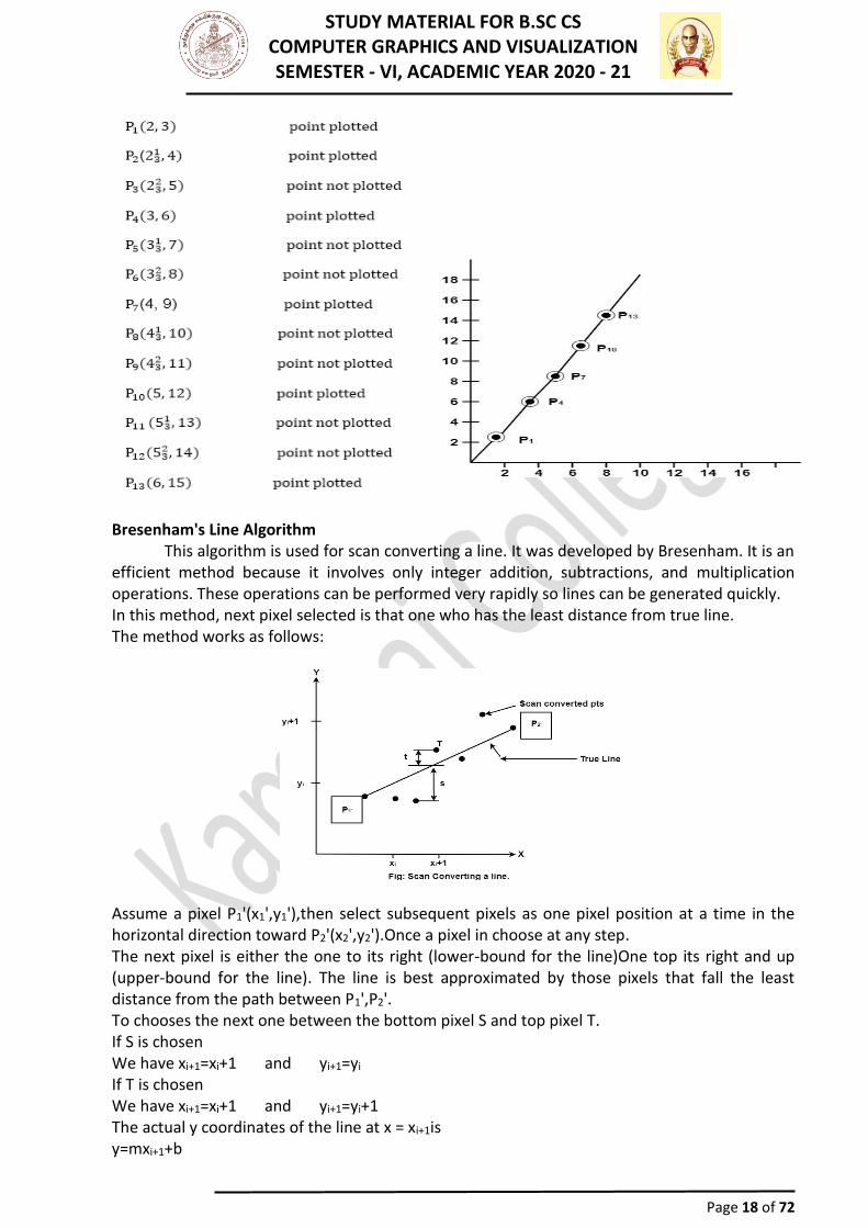
DDA Algorithm: Step1: Start Algorithm Step2: Declare x1,y1,x2,y2,dx,dy,x,y as integer variables. Step3: Enter value of x1,y1,x2,y2. Step4: Calculate dx = x2-x1 Step5: Calculate dy = y2-y1 Step6: If ABS (dx) > ABS (dy) Then step = abs (dx) Else Step7:xinc=dx/step yinc=dy/step assign x = x1 assign y = y1 Step8: Set pixel (x, y) Step9: x = x + xinc y = y + yinc Set pixels (Round (x), Round (y)) Step10: Repeat step 9 until x = x2 Step11: End Algorithm Example: If a line is drawn from (2, 3) to (6, 15) with use of DDA. How many points will needed to generate such line? Solution: P1 (2,3) P11 (6,15) x1=2 y1=3 x2= 6 y2=15 dx = 6 - 2 = 4 dy = 15 - 3 = 12
m =
For calculating next value of x takes x = x +
STUDY MATERIAL FOR B.SC CS COMPUTER GRAPHICS AND VISUALIZATION SEMESTER - VI, ACADEMIC YEAR 2020 - 21
Page 18 of 72
Bresenham's Line Algorithm This algorithm is used for scan converting a line. It was developed by Bresenham. It is an
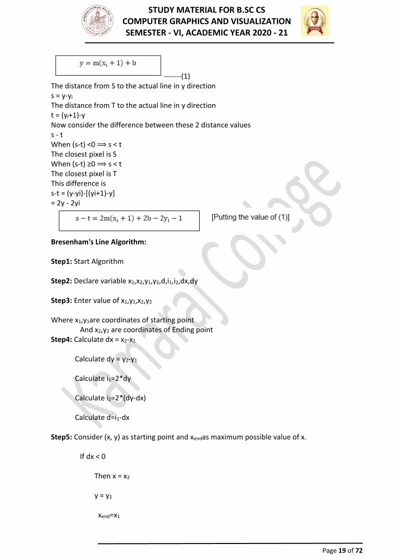
efficient method because it involves only integer addition, subtractions, and multiplication operations. These operations can be performed very rapidly so lines can be generated quickly. In this method, next pixel selected is that one who has the least distance from true line. The method works as follows:
Assume a pixel P1'(x1',y1'),then select subsequent pixels as one pixel position at a time in the horizontal direction toward P2'(x2',y2').Once a pixel in choose at any step. The next pixel is either the one to its right (lower-bound for the line)One top its right and up (upper-bound for the line). The line is best approximated by those pixels that fall the least distance from the path between P1',P2'. To chooses the next one between the bottom pixel S and top pixel T. If S is chosen We have xi+1=xi+1 and yi+1=yi
If T is chosen We have xi+1=xi+1 and yi+1=yi+1 The actual y coordinates of the line at x = xi+1is y=mxi+1+b
STUDY MATERIAL FOR B.SC CS COMPUTER GRAPHICS AND VISUALIZATION SEMESTER - VI, ACADEMIC YEAR 2020 - 21
Page 19 of 72
-------(1) The distance from S to the actual line in y direction s = y-yi The distance from T to the actual line in y direction t = (yi+1)-y Now consider the difference between these 2 distance values s - t When (s-t) <0 ⟹ s < t The closest pixel is S When (s-t) ≥0 ⟹ s < t The closest pixel is T This difference is s-t = (y-yi)-[(yi+1)-y] = 2y - 2yi
Bresenham's Line Algorithm: Step1: Start Algorithm Step2: Declare variable x1,x2,y1,y2,d,i1,i2,dx,dy Step3: Enter value of x1,y1,x2,y2
Where x1,y1are coordinates of starting point And x2,y2 are coordinates of Ending point Step4: Calculate dx = x2-x1
Calculate dy = y2-y1
Calculate i1=2*dy
Calculate i2=2*(dy-dx)
Calculate d=i1-dx
Step5: Consider (x, y) as starting point and xendas maximum possible value of x. If dx < 0 Then x = x2
y = y2
xend=x1
STUDY MATERIAL FOR B.SC CS COMPUTER GRAPHICS AND VISUALIZATION SEMESTER - VI, ACADEMIC YEAR 2020 - 21
Page 20 of 72
If dx > 0 Then x = x1
y = y1
xend=x2 Step6: Generate point at (x,y)coordinates. Step7: Check if whole line is generated. If x > = xend
Stop. Step8: Calculate co-ordinates of the next pixel If d < 0 Then d = d + i1
If d ≥ 0 Then d = d + i2
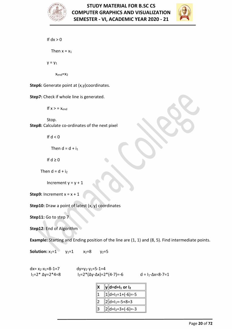
Increment y = y + 1 Step9: Increment x = x + 1 Step10: Draw a point of latest (x, y) coordinates Step11: Go to step 7 Step12: End of Algorithm Example: Starting and Ending position of the line are (1, 1) and (8, 5). Find intermediate points. Solution: x1=1 y1=1 x2=8 y2=5 dx= x2-x1=8-1=7 dy=y2-y1=5-1=4 I1=2* ∆y=2*4=8 I2=2*(∆y-∆x)=2*(4-7)=-6 d = I1-∆x=8-7=1
X y d=d+I1 or I2
1 1 d+I2=1+(-6)=-5
2 2 d+I1=-5+8=3
3 2 d+I2=3+(-6)=-3
STUDY MATERIAL FOR B.SC CS COMPUTER GRAPHICS AND VISUALIZATION SEMESTER - VI, ACADEMIC YEAR 2020 - 21
Page 21 of 72
4 3 d+I1=-3+8=5
5 3 d+I2=5+(-6)=-1
6 4 d+I1=-1+8=7
7 4 d+I2=7+(-6)=1
8 5
Advantage:
1. It involves only integer arithmetic, so it is simple. 2. It avoids the generation of duplicate points. 3. It can be implemented using hardware because it does not use multiplication and
division. 4. It is faster as compared to DDA (Digital Differential Analyzer) because it does not involve
floating point calculations like DDA Algorithm. Disadvantage:
1. This algorithm is meant for basic line drawing only Initializing is not a part of Bresenham's line algorithm. So to draw smooth lines, you should want to look into a different algorithm.
STUDY MATERIAL FOR B.SC CS COMPUTER GRAPHICS AND VISUALIZATION SEMESTER - VI, ACADEMIC YEAR 2020 - 21
Page 22 of 72
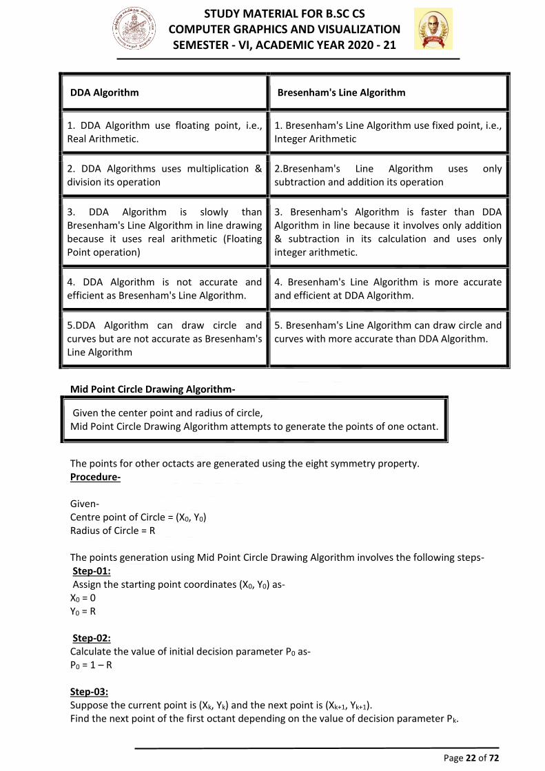
DDA Algorithm Bresenham's Line Algorithm
1. DDA Algorithm use floating point, i.e., Real Arithmetic.
1. Bresenham's Line Algorithm use fixed point, i.e., Integer Arithmetic
2. DDA Algorithms uses multiplication & division its operation
2.Bresenham's Line Algorithm uses only subtraction and addition its operation
3. DDA Algorithm is slowly than Bresenham's Line Algorithm in line drawing because it uses real arithmetic (Floating Point operation)
3. Bresenham's Algorithm is faster than DDA Algorithm in line because it involves only addition & subtraction in its calculation and uses only integer arithmetic.
4. DDA Algorithm is not accurate and efficient as Bresenham's Line Algorithm.
4. Bresenham's Line Algorithm is more accurate and efficient at DDA Algorithm.
5.DDA Algorithm can draw circle and curves but are not accurate as Bresenham's Line Algorithm
5. Bresenham's Line Algorithm can draw circle and curves with more accurate than DDA Algorithm.
Mid Point Circle Drawing Algorithm-
Given the center point and radius of circle, Mid Point Circle Drawing Algorithm attempts to generate the points of one octant.
The points for other octacts are generated using the eight symmetry property. Procedure- Given- Centre point of Circle = (X0, Y0) Radius of Circle = R The points generation using Mid Point Circle Drawing Algorithm involves the following steps- Step-01: Assign the starting point coordinates (X0, Y0) as- X0 = 0 Y0 = R Step-02: Calculate the value of initial decision parameter P0 as- P0 = 1 – R Step-03: Suppose the current point is (Xk, Yk) and the next point is (Xk+1, Yk+1). Find the next point of the first octant depending on the value of decision parameter Pk.
STUDY MATERIAL FOR B.SC CS COMPUTER GRAPHICS AND VISUALIZATION SEMESTER - VI, ACADEMIC YEAR 2020 - 21
Page 23 of 72
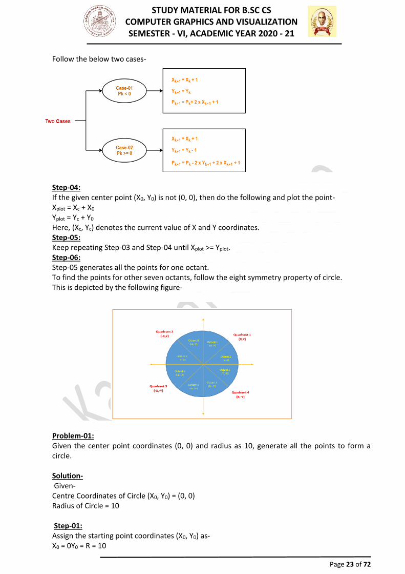
Follow the below two cases-
Step-04: If the given center point (X0, Y0) is not (0, 0), then do the following and plot the point- Xplot = Xc + X0 Yplot = Yc + Y0 Here, (Xc, Yc) denotes the current value of X and Y coordinates. Step-05: Keep repeating Step-03 and Step-04 until Xplot >= Yplot. Step-06: Step-05 generates all the points for one octant. To find the points for other seven octants, follow the eight symmetry property of circle. This is depicted by the following figure-
Problem-01: Given the center point coordinates (0, 0) and radius as 10, generate all the points to form a circle. Solution- Given- Centre Coordinates of Circle (X0, Y0) = (0, 0) Radius of Circle = 10 Step-01: Assign the starting point coordinates (X0, Y0) as- X0 = 0Y0 = R = 10
STUDY MATERIAL FOR B.SC CS COMPUTER GRAPHICS AND VISUALIZATION SEMESTER - VI, ACADEMIC YEAR 2020 - 21
Page 24 of 72
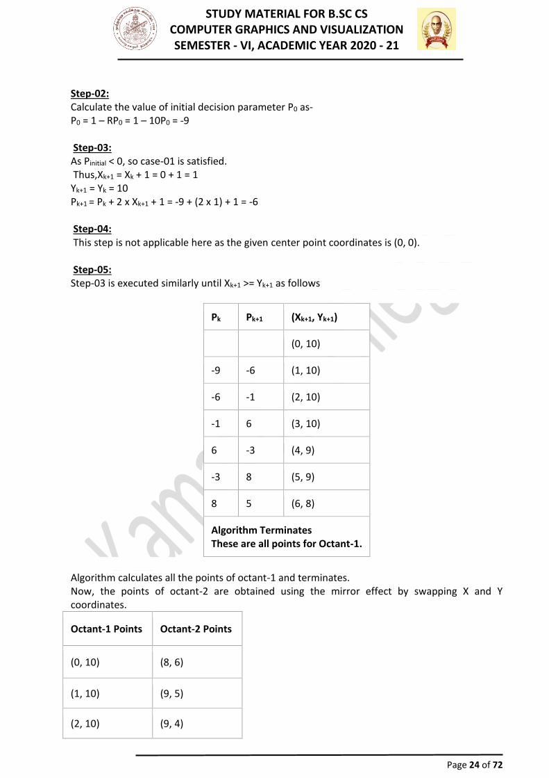
Step-02: Calculate the value of initial decision parameter P0 as- P0 = 1 – RP0 = 1 – 10P0 = -9 Step-03: As Pinitial < 0, so case-01 is satisfied. Thus,Xk+1 = Xk + 1 = 0 + 1 = 1 Yk+1 = Yk = 10 Pk+1 = Pk + 2 x Xk+1 + 1 = -9 + (2 x 1) + 1 = -6 Step-04: This step is not applicable here as the given center point coordinates is (0, 0). Step-05: Step-03 is executed similarly until Xk+1 >= Yk+1 as follows
Pk Pk+1 (Xk+1, Yk+1)
(0, 10)
-9 -6 (1, 10)
-6 -1 (2, 10)
-1 6 (3, 10)
6 -3 (4, 9)
-3 8 (5, 9)
8 5 (6, 8)
Algorithm Terminates These are all points for Octant-1.
Algorithm calculates all the points of octant-1 and terminates. Now, the points of octant-2 are obtained using the mirror effect by swapping X and Y coordinates.
Octant-1 Points Octant-2 Points
(0, 10) (8, 6)
(1, 10) (9, 5)
(2, 10) (9, 4)
STUDY MATERIAL FOR B.SC CS COMPUTER GRAPHICS AND VISUALIZATION SEMESTER - VI, ACADEMIC YEAR 2020 - 21
Page 25 of 72
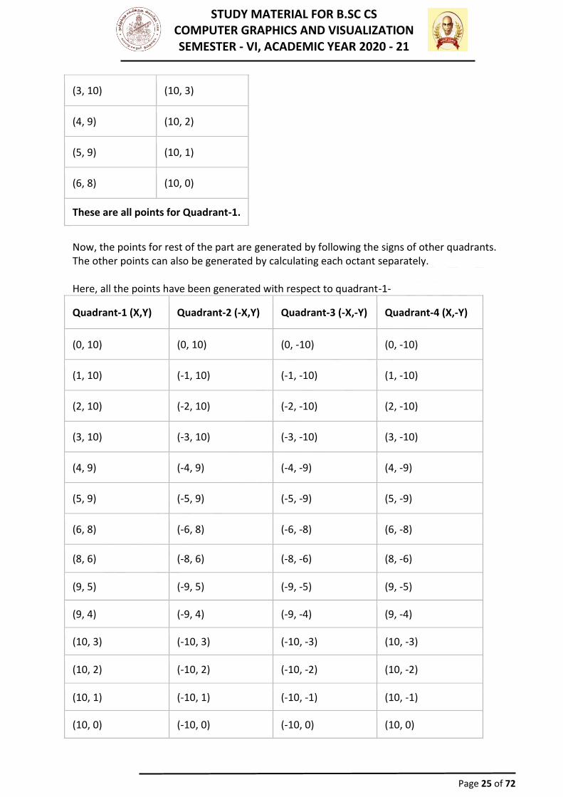
(3, 10) (10, 3)
(4, 9) (10, 2)
(5, 9) (10, 1)
(6, 8) (10, 0)
These are all points for Quadrant-1.
Now, the points for rest of the part are generated by following the signs of other quadrants. The other points can also be generated by calculating each octant separately. Here, all the points have been generated with respect to quadrant-1-
Quadrant-1 (X,Y) Quadrant-2 (-X,Y) Quadrant-3 (-X,-Y) Quadrant-4 (X,-Y)
(0, 10) (0, 10) (0, -10) (0, -10)
(1, 10) (-1, 10) (-1, -10) (1, -10)
(2, 10) (-2, 10) (-2, -10) (2, -10)
(3, 10) (-3, 10) (-3, -10) (3, -10)
(4, 9) (-4, 9) (-4, -9) (4, -9)
(5, 9) (-5, 9) (-5, -9) (5, -9)
(6, 8) (-6, 8) (-6, -8) (6, -8)
(8, 6) (-8, 6) (-8, -6) (8, -6)
(9, 5) (-9, 5) (-9, -5) (9, -5)
(9, 4) (-9, 4) (-9, -4) (9, -4)
(10, 3) (-10, 3) (-10, -3) (10, -3)
(10, 2) (-10, 2) (-10, -2) (10, -2)
(10, 1) (-10, 1) (-10, -1) (10, -1)
(10, 0) (-10, 0) (-10, 0) (10, 0)
STUDY MATERIAL FOR B.SC CS COMPUTER GRAPHICS AND VISUALIZATION SEMESTER - VI, ACADEMIC YEAR 2020 - 21
Page 26 of 72
These are all points of the Circle.
Advantages of Mid-Point Circle Drawing Algorithm-
➢ It is a powerful and efficient algorithm. ➢ The entire algorithm is based on the simple equation of circle X2 + Y2 = R2. ➢ It is easy to implement from the programmer’s perspective. ➢ This algorithm is used to generate curves on raster displays.
Disadvantages of Mid-Point Circle Drawing Algorithm-
➢ Accuracy of the generating points is an issue in this algorithm. ➢ The circle generated by this algorithm is not smooth. ➢ This algorithm is time consuming.
Important Points • Circle drawing algorithms take the advantage of 8 symmetry property of circle. • Every circle has 8 octants and the circle drawing algorithm generates all the points for
one octant. • The points for other 7 octants are generated by changing the sign towards X and Y
coordinates. • To take the advantage of 8 symmetry property, the circle must be formed assuming that
the center point coordinates is (0, 0). • If the center coordinates are other than (0, 0), then we add the X and Y coordinate
values with each point of circle with the coordinate values generated by assuming (0, 0) as centre point.
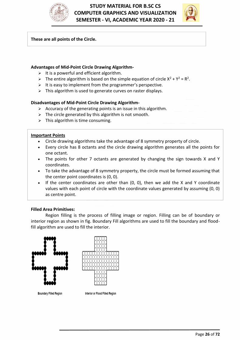
Filled Area Primitives:
Region filling is the process of filling image or region. Filling can be of boundary or interior region as shown in fig. Boundary Fill algorithms are used to fill the boundary and flood-fill algorithm are used to fill the interior.
STUDY MATERIAL FOR B.SC CS COMPUTER GRAPHICS AND VISUALIZATION SEMESTER - VI, ACADEMIC YEAR 2020 - 21
Page 27 of 72
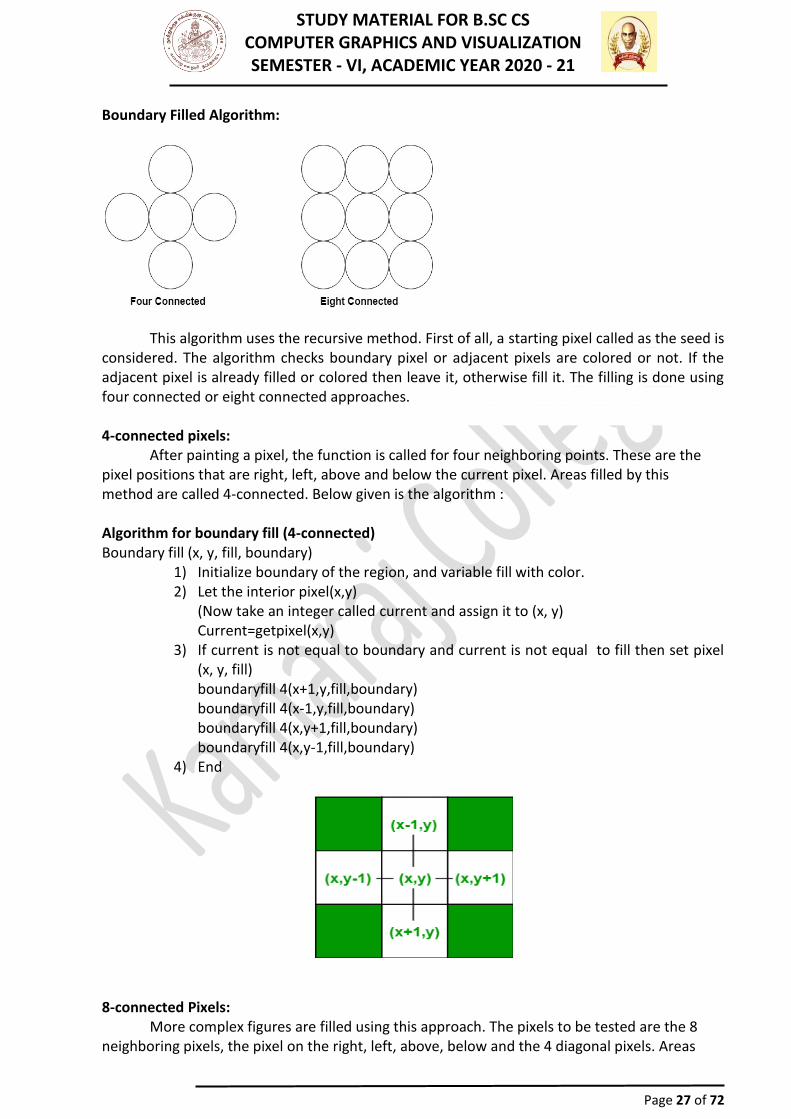
Boundary Filled Algorithm:
This algorithm uses the recursive method. First of all, a starting pixel called as the seed is
considered. The algorithm checks boundary pixel or adjacent pixels are colored or not. If the adjacent pixel is already filled or colored then leave it, otherwise fill it. The filling is done using four connected or eight connected approaches. 4-connected pixels:
After painting a pixel, the function is called for four neighboring points. These are the pixel positions that are right, left, above and below the current pixel. Areas filled by this method are called 4-connected. Below given is the algorithm : Algorithm for boundary fill (4-connected) Boundary fill (x, y, fill, boundary)
1) Initialize boundary of the region, and variable fill with color. 2) Let the interior pixel(x,y)
(Now take an integer called current and assign it to (x, y) Current=getpixel(x,y)
3) If current is not equal to boundary and current is not equal to fill then set pixel (x, y, fill) boundaryfill 4(x+1,y,fill,boundary) boundaryfill 4(x-1,y,fill,boundary) boundaryfill 4(x,y+1,fill,boundary) boundaryfill 4(x,y-1,fill,boundary)
4) End
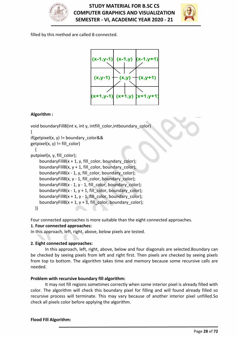
8-connected Pixels:
More complex figures are filled using this approach. The pixels to be tested are the 8 neighboring pixels, the pixel on the right, left, above, below and the 4 diagonal pixels. Areas
STUDY MATERIAL FOR B.SC CS COMPUTER GRAPHICS AND VISUALIZATION SEMESTER - VI, ACADEMIC YEAR 2020 - 21
Page 28 of 72
filled by this method are called 8-connected.
Algorithm : void boundaryFill8(int x, int y, intfill_color,intboundary_color) { if(getpixel(x, y) != boundary_color&& getpixel(x, y) != fill_color) { putpixel(x, y, fill_color); boundaryFill8(x + 1, y, fill_color, boundary_color); boundaryFill8(x, y + 1, fill_color, boundary_color); boundaryFill8(x - 1, y, fill_color, boundary_color); boundaryFill8(x, y - 1, fill_color, boundary_color); boundaryFill8(x - 1, y - 1, fill_color, boundary_color); boundaryFill8(x - 1, y + 1, fill_color, boundary_color); boundaryFill8(x + 1, y - 1, fill_color, boundary_color); boundaryFill8(x + 1, y + 1, fill_color, boundary_color); }} Four connected approaches is more suitable than the eight connected approaches. 1. Four connected approaches: In this approach, left, right, above, below pixels are tested. 2. Eight connected approaches:
In this approach, left, right, above, below and four diagonals are selected.Boundary can be checked by seeing pixels from left and right first. Then pixels are checked by seeing pixels from top to bottom. The algorithm takes time and memory because some recursive calls are needed. Problem with recursive boundary fill algorithm:
It may not fill regions sometimes correctly when some interior pixel is already filled with color. The algorithm will check this boundary pixel for filling and will found already filled so recursive process will terminate. This may vary because of another interior pixel unfilled.So check all pixels color before applying the algorithm. Flood Fill Algorithm:
STUDY MATERIAL FOR B.SC CS COMPUTER GRAPHICS AND VISUALIZATION SEMESTER - VI, ACADEMIC YEAR 2020 - 21
Page 29 of 72
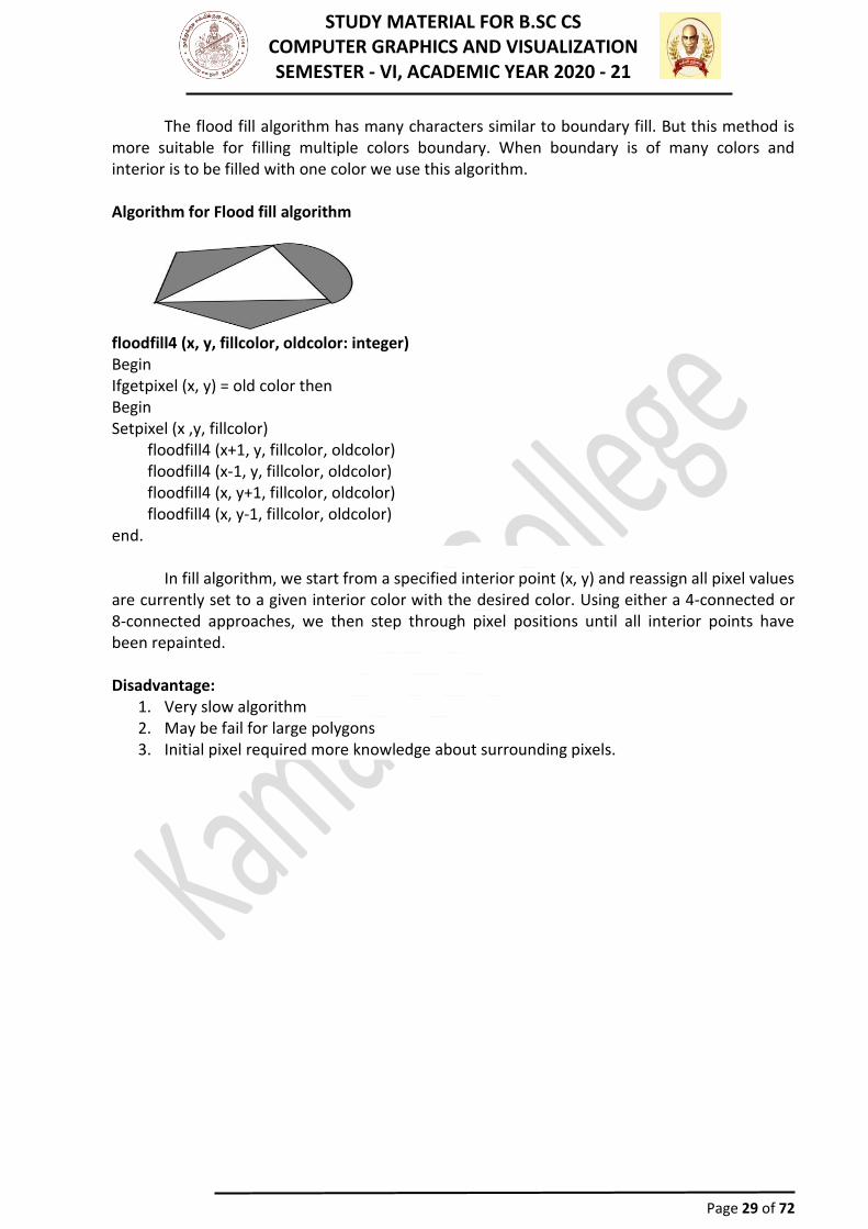
The flood fill algorithm has many characters similar to boundary fill. But this method is more suitable for filling multiple colors boundary. When boundary is of many colors and interior is to be filled with one color we use this algorithm. Algorithm for Flood fill algorithm
floodfill4 (x, y, fillcolor, oldcolor: integer) Begin Ifgetpixel (x, y) = old color then Begin Setpixel (x ,y, fillcolor) floodfill4 (x+1, y, fillcolor, oldcolor) floodfill4 (x-1, y, fillcolor, oldcolor) floodfill4 (x, y+1, fillcolor, oldcolor) floodfill4 (x, y-1, fillcolor, oldcolor) end.
In fill algorithm, we start from a specified interior point (x, y) and reassign all pixel values are currently set to a given interior color with the desired color. Using either a 4-connected or 8-connected approaches, we then step through pixel positions until all interior points have been repainted. Disadvantage:
1. Very slow algorithm 2. May be fail for large polygons 3. Initial pixel required more knowledge about surrounding pixels.
STUDY MATERIAL FOR B.SC CS COMPUTER GRAPHICS AND VISUALIZATION SEMESTER - VI, ACADEMIC YEAR 2020 - 21
Page 30 of 72
UNIT - II ATTRIBUTES OF OUTPUT PRIMITIVES
Attributes of OutputPrimitives
Any parameter that affects the way a primitive is to be displayed is referred to as an attribute parameter. Example attribute parameters are color, size etc. A line drawing function for example could contain parameter to set color, width and other properties.
1. LineAttributes 2. CurveAttributes 3. Color and GrayscaleLevels 4. Area FillAttributes 5. CharacterAttributes 6. BundledAttributes
Line Attributes
Basic attributes of a straight line segment are its type, its width, and its color. In some graphics packages, lines can also be displayed using selected pen or brush options
➢ LineType ➢ LineWidth ➢ Pen and BrushOptions ➢ LineColor
Line type
Possible selection of line type attribute includes solid lines, dashed lines and dotted lines. To set line type attributes in a PHIGSapplication program, a user invokes the functionsetLinetype (lt)
Where parameter lt is assigned a positive integer value of 1, 2, 3 or 4 to generate lines that aresolid, dashed, dash dotted respectively. Other values for line type parameter it could be used to display variations in dot-dash patterns. Line width
Implementation of line width option depends on the capabilities of the output device to set the line width attributes.
SetLinewidthScaleFactor (lw) Line width parameter lw is assigned a positive number to indicate the relative
width of line to be displayed. A value of 1 specifies a standard width line. A user could set lw to a value of 0.5 to plot a line whose width is half that of the standard line. Values greater than 1 produce lines thicker than the standard. Line Cap
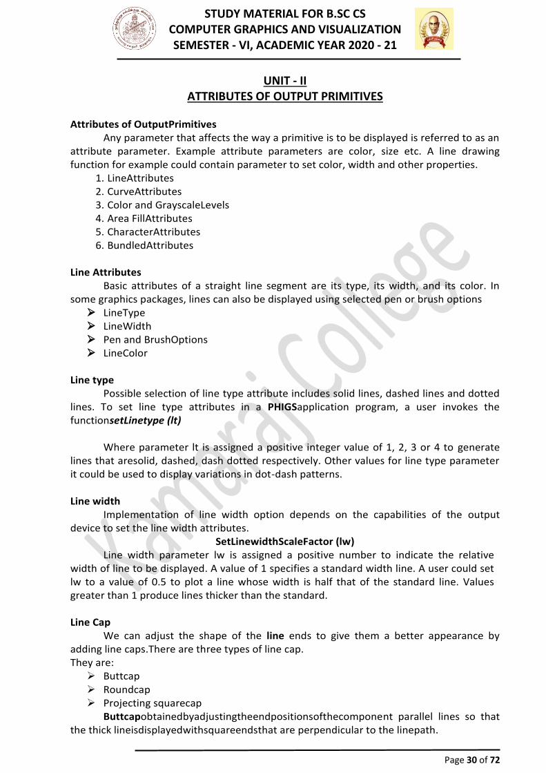
We can adjust the shape of the line ends to give them a better appearance by adding line caps.There are three types of line cap. They are:
➢ Buttcap ➢ Roundcap ➢ Projecting squarecap
Buttcapobtainedbyadjustingtheendpositionsofthecomponent parallel lines so that the thick lineisdisplayedwithsquareendsthat are perpendicular to the linepath.
STUDY MATERIAL FOR B.SC CS COMPUTER GRAPHICS AND VISUALIZATION SEMESTER - VI, ACADEMIC YEAR 2020 - 21
Page 31 of 72
Round cap obtained by adding a filled semicircle to each butt cap. The circular arcs
are centered on the line endpoints and have a diameter equal to the line thickness.
Projecting square cap extend the line and add butt caps that are positioned one-half of the line width beyond the specified endpoints.
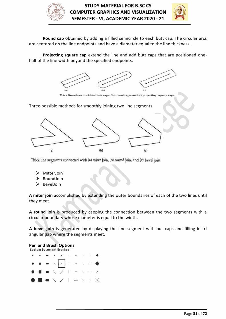
Three possible methods for smoothly joining two line segments
➢ MitterJoin ➢ RoundJoin ➢ BevelJoin
A miter join accomplished by extending the outer boundaries of each of the two lines until they meet. A round join is produced by capping the connection between the two segments with a circular boundary whose diameter is equal to the width. A bevel join is generated by displaying the line segment with but caps and filling in tri angular gap where the segments meet. Pen and Brush Options
STUDY MATERIAL FOR B.SC CS COMPUTER GRAPHICS AND VISUALIZATION SEMESTER - VI, ACADEMIC YEAR 2020 - 21
Page 32 of 72
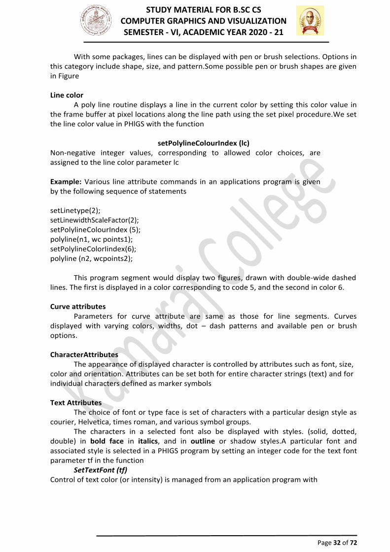
With some packages, lines can be displayed with pen or brush selections. Options in this category include shape, size, and pattern.Some possible pen or brush shapes are given in Figure Line color
A poly line routine displays a line in the current color by setting this color value in the frame buffer at pixel locations along the line path using the set pixel procedure.We set the line color value in PHlGS with the function
setPolylineColourIndex (lc)
Non-negative integer values, corresponding to allowed color choices, are assigned to the line color parameter lc Example: Various line attribute commands in an applications program is given by the following sequence of statements setLinetype(2); setLinewidthScaleFactor(2); setPolylineColourIndex (5); polyline(n1, wc points1); setPolylineColorIindex(6); polyline (n2, wcpoints2);
This program segment would display two figures, drawn with double-wide dashed lines. The first is displayed in a color corresponding to code 5, and the second in color 6. Curve attributes
Parameters for curve attribute are same as those for line segments. Curves displayed with varying colors, widths, dot – dash patterns and available pen or brush options. CharacterAttributes
The appearance of displayed character is controlled by attributes such as font, size, color and orientation. Attributes can be set both for entire character strings (text) and for individual characters defined as marker symbols Text Attributes
The choice of font or type face is set of characters with a particular design style as courier, Helvetica, times roman, and various symbol groups.
The characters in a selected font also be displayed with styles. (solid, dotted, double) in bold face in italics, and in outline or shadow styles.A particular font and associated style is selected in a PHIGS program by setting an integer code for the text font parameter tf in the function
SetTextFont (tf) Control of text color (or intensity) is managed from an application program with
STUDY MATERIAL FOR B.SC CS COMPUTER GRAPHICS AND VISUALIZATION SEMESTER - VI, ACADEMIC YEAR 2020 - 21
Page 33 of 72
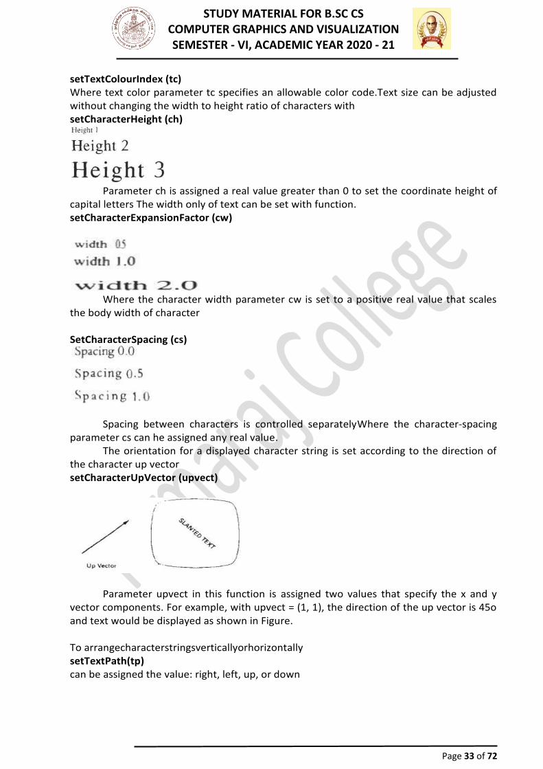
setTextColourIndex (tc) Where text color parameter tc specifies an allowable color code.Text size can be adjusted without changing the width to height ratio of characters with setCharacterHeight (ch)
Parameter ch is assigned a real value greater than 0 to set the coordinate height of
capital letters The width only of text can be set with function. setCharacterExpansionFactor (cw)
Where the character width parameter cw is set to a positive real value that scales
the body width of character SetCharacterSpacing (cs)
Spacing between characters is controlled separatelyWhere the character-spacing parameter cs can he assigned any real value.
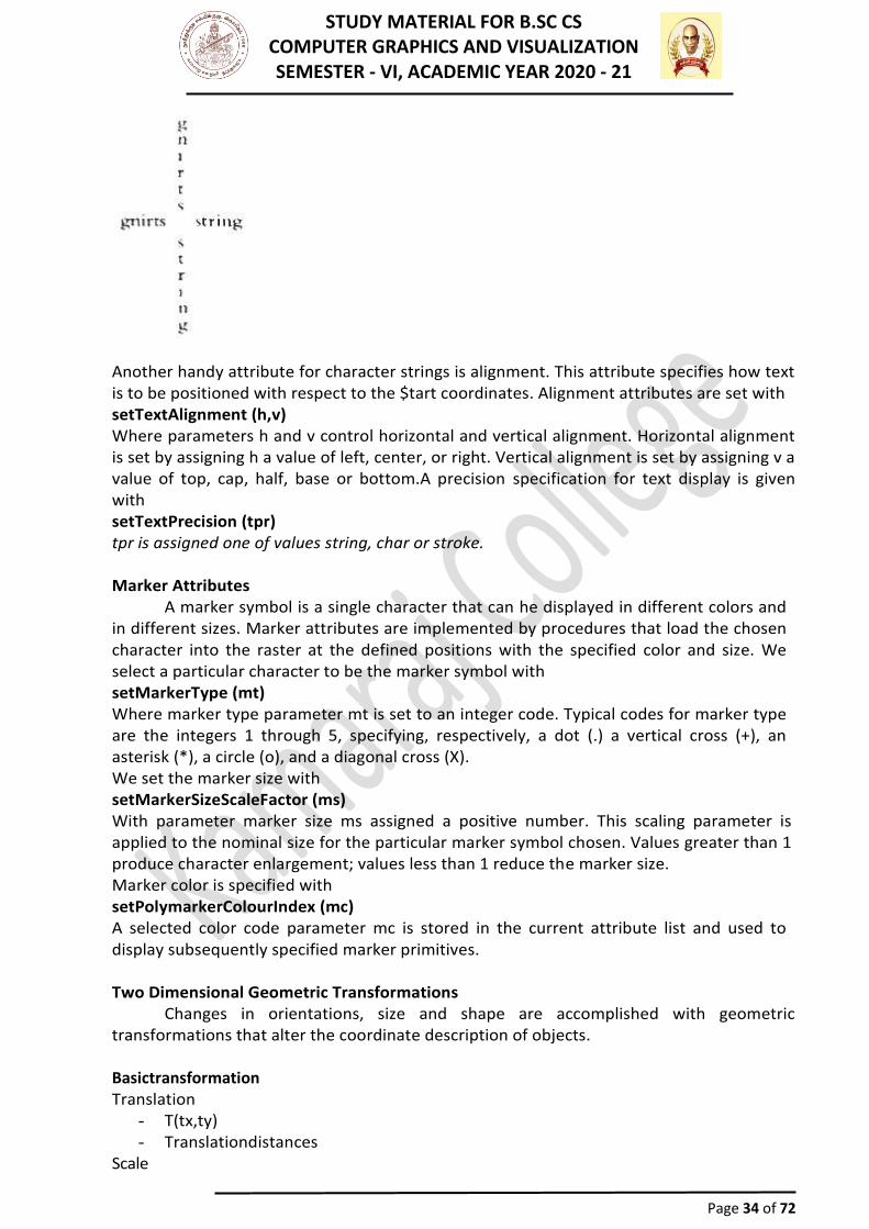
The orientation for a displayed character string is set according to the direction of the character up vector setCharacterUpVector (upvect)
Parameter upvect in this function is assigned two values that specify the x and y vector components. For example, with upvect = (1, 1), the direction of the up vector is 45o and text would be displayed as shown in Figure. To arrangecharacterstringsverticallyorhorizontally setTextPath(tp) can be assigned the value: right, left, up, or down
STUDY MATERIAL FOR B.SC CS COMPUTER GRAPHICS AND VISUALIZATION SEMESTER - VI, ACADEMIC YEAR 2020 - 21
Page 34 of 72
Another handy attribute for character strings is alignment. This attribute specifies how text is to be positioned with respect to the $tart coordinates. Alignment attributes are set with setTextAlignment (h,v) Where parameters h and v control horizontal and vertical alignment. Horizontal alignment is set by assigning h a value of left, center, or right. Vertical alignment is set by assigning v a value of top, cap, half, base or bottom.A precision specification for text display is given with setTextPrecision (tpr) tpr is assigned one of values string, char or stroke. Marker Attributes
A marker symbol is a single character that can he displayed in different colors and in different sizes. Marker attributes are implemented by procedures that load the chosen character into the raster at the defined positions with the specified color and size. We select a particular character to be the marker symbol with setMarkerType (mt) Where marker type parameter mt is set to an integer code. Typical codes for marker type are the integers 1 through 5, specifying, respectively, a dot (.) a vertical cross (+), an asterisk (*), a circle (o), and a diagonal cross (X). We set the marker size with setMarkerSizeScaleFactor (ms) With parameter marker size ms assigned a positive number. This scaling parameter is applied to the nominal size for the particular marker symbol chosen. Values greater than 1 produce character enlargement; values less than 1 reduce the marker size. Marker color is specified with setPolymarkerColourIndex (mc) A selected color code parameter mc is stored in the current attribute list and used to display subsequently specified marker primitives. Two Dimensional Geometric Transformations
Changes in orientations, size and shape are accomplished with geometric transformations that alter the coordinate description of objects. Basictransformation Translation
- T(tx,ty) - Translationdistances
Scale
STUDY MATERIAL FOR B.SC CS COMPUTER GRAPHICS AND VISUALIZATION SEMESTER - VI, ACADEMIC YEAR 2020 - 21
Page 35 of 72
- S(sx,sy) - Scalefactors
Rotation - R() - Rotationangle
Translation
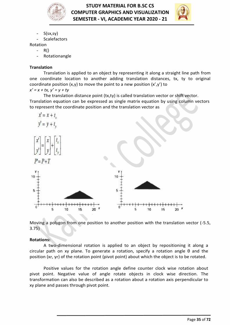
Translation is applied to an object by representing it along a straight line path from one coordinate location to another adding translation distances, tx, ty to original coordinate position (x,y) to move the point to a new position (x’,y’) to x’ = x + tx, y’ = y + ty
The translation distance point (tx,ty) is called translation vector or shift vector. Translation equation can be expressed as single matrix equation by using column vectors to represent the coordinate position and the translation vector as
Moving a polygon from one position to another position with the translation vector (-5.5, 3.75) Rotations:
A two-dimensional rotation is applied to an object by repositioning it along a circular path on xy plane. To generate a rotation, specify a rotation angle θ and the position (xr, yr) of the rotation point (pivot point) about which the object is to be rotated.
Positive values for the rotation angle define counter clock wise rotation about
pivot point. Negative value of angle rotate objects in clock wise direction. The transformation can also be described as a rotation about a rotation axis perpendicular to xy plane and passes through pivot point.
STUDY MATERIAL FOR B.SC CS COMPUTER GRAPHICS AND VISUALIZATION SEMESTER - VI, ACADEMIC YEAR 2020 - 21
Page 36 of 72
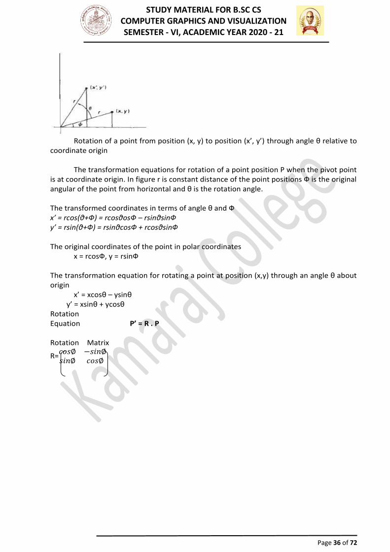
Rotation of a point from position (x, y) to position (x’, y’) through angle θ relative to
coordinate origin
The transformation equations for rotation of a point position P when the pivot point is at coordinate origin. In figure r is constant distance of the point positions Ф is the original angular of the point from horizontal and θ is the rotation angle. The transformed coordinates in terms of angle θ and Ф x’ = rcos(θ+Ф) = rcosθosФ – rsinθsinФ y’ = rsin(θ+Ф) = rsinθcosФ + rcosθsinФ The original coordinates of the point in polar coordinates x = rcosФ, y = rsinФ The transformation equation for rotating a point at position (x,y) through an angle θ about origin x’ = xcosθ – ysinθ
y’ = xsinθ + ycosθRotation Equation Rotation Matrix
R=𝑐𝑜𝑠∅ −𝑠𝑖𝑛∅𝑠𝑖𝑛∅ 𝑐𝑜𝑠∅
P’ = R . P
STUDY MATERIAL FOR B.SC CS COMPUTER GRAPHICS AND VISUALIZATION SEMESTER - VI, ACADEMIC YEAR 2020 - 21
Page 37 of 72
Note: Positive values for the rotation angle define counterclockwise rotations about the rotation point and negative values rotate objects in the clockwise. Scaling
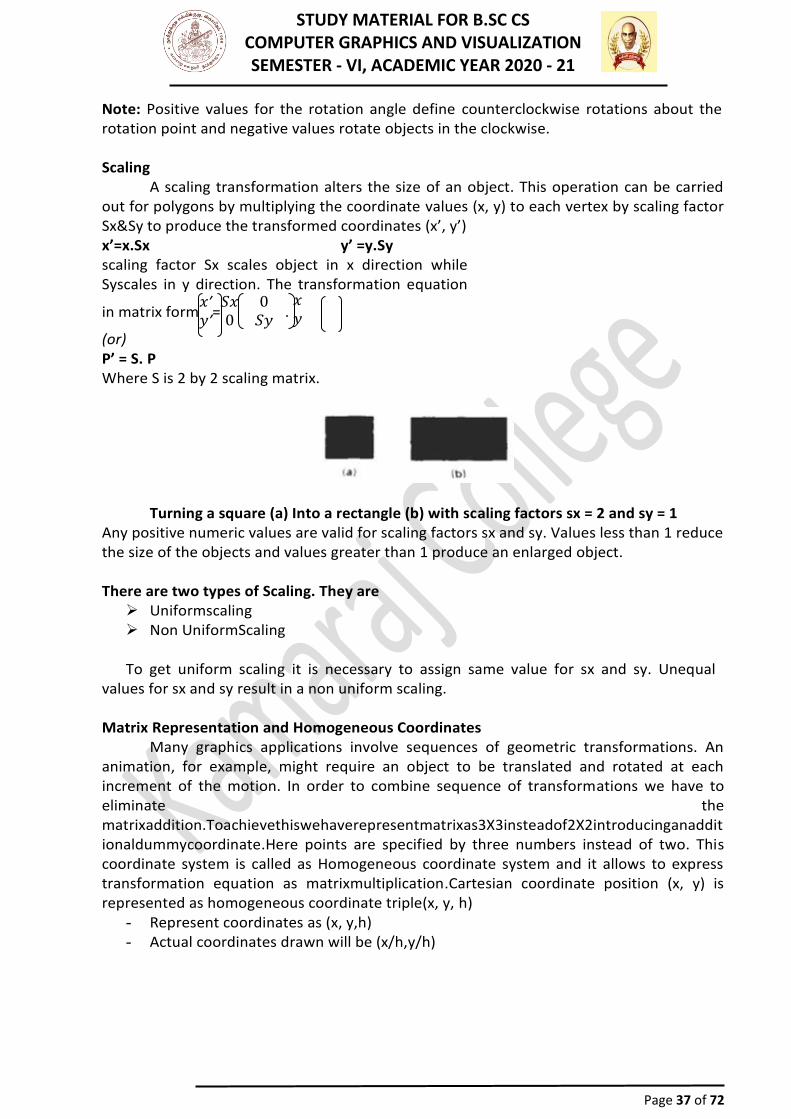
A scaling transformation alters the size of an object. This operation can be carried out for polygons by multiplying the coordinate values (x, y) to each vertex by scaling factor Sx&Sy to produce the transformed coordinates (x’, y’) x’=x.Sx y’ =y.Sy scaling factor Sx scales object in x direction while Syscales in y direction. The transformation equation
in matrix form𝑥′𝑦′
=𝑆𝑥 00 𝑆𝑦
. 𝑥𝑦
(or) P’ = S. P Where S is 2 by 2 scaling matrix.
Turning a square (a) Into a rectangle (b) with scaling factors sx = 2 and sy = 1 Any positive numeric values are valid for scaling factors sx and sy. Values less than 1 reduce the size of the objects and values greater than 1 produce an enlarged object. There are two types of Scaling. They are
➢ Uniformscaling ➢ Non UniformScaling To get uniform scaling it is necessary to assign same value for sx and sy. Unequal
values for sx and sy result in a non uniform scaling. Matrix Representation and Homogeneous Coordinates
Many graphics applications involve sequences of geometric transformations. An animation, for example, might require an object to be translated and rotated at each increment of the motion. In order to combine sequence of transformations we have to eliminate the matrixaddition.Toachievethiswehaverepresentmatrixas3X3insteadof2X2introducinganadditionaldummycoordinate.Here points are specified by three numbers instead of two. This coordinate system is called as Homogeneous coordinate system and it allows to express transformation equation as matrixmultiplication.Cartesian coordinate position (x, y) is represented as homogeneous coordinate triple(x, y, h)
- Represent coordinates as (x, y,h) - Actual coordinates drawn will be (x/h,y/h)
STUDY MATERIAL FOR B.SC CS COMPUTER GRAPHICS AND VISUALIZATION SEMESTER - VI, ACADEMIC YEAR 2020 - 21
Page 38 of 72
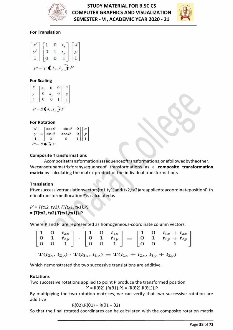
For Translation
For Scaling
For Rotation
Composite Transformations
Acompositetransformationisasequenceoftransformations;onefollowedbytheother. Wecansetupamatrixforanysequenceof transformations as a composite transformation matrix by calculating the matrix product of the individual transformations Translation Iftwosuccessivetranslationvectors(tx1,ty1)and(tx2,ty2)areappliedtoacoordinatepositionP,thefinaltransformedlocationP’is calculatedas P’ = T(tx2, ty2). {T(tx1, ty1).P} = {T(tx2, ty2).T(tx1,ty1)}.P Where P and P’ are represented as homogeneous-coordinate column vectors.
Which demonstrated the two successive translations are additive. Rotations Two successive rotations applied to point P produce the transformed position
P’ = R(θ2).{R(θ1).P} = {R(θ2).R(θ1)}.P By multiplying the two rotation matrices, we can verify that two successive rotation are additive
R(θ2).R(θ1) = R(θ1 + θ2) So that the final rotated coordinates can be calculated with the composite rotation matrix
STUDY MATERIAL FOR B.SC CS COMPUTER GRAPHICS AND VISUALIZATION SEMESTER - VI, ACADEMIC YEAR 2020 - 21
Page 39 of 72
as
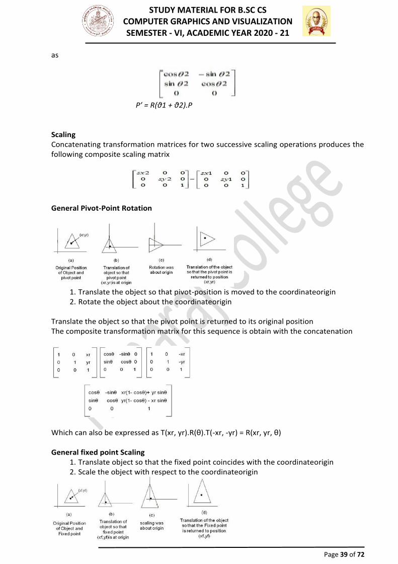
P’ = R(θ1 + θ2).P Scaling Concatenating transformation matrices for two successive scaling operations produces the following composite scaling matrix
General Pivot-Point Rotation
1. Translate the object so that pivot-position is moved to the coordinateorigin 2. Rotate the object about the coordinateorigin
Translate the object so that the pivot point is returned to its original position The composite transformation matrix for this sequence is obtain with the concatenation
Which can also be expressed as T(xr, yr).R(θ).T(-xr, -yr) = R(xr, yr, θ) General fixed point Scaling
1. Translate object so that the fixed point coincides with the coordinateorigin 2. Scale the object with respect to the coordinateorigin
STUDY MATERIAL FOR B.SC CS COMPUTER GRAPHICS AND VISUALIZATION SEMESTER - VI, ACADEMIC YEAR 2020 - 21
Page 40 of 72
Use the inverse translation of step 1 to return the object to its original position Concatenating the matrices for these three operations produces the required scaling matix
Can also be expressed as T(xf, yf).S(sx, sy).T(-xf, -yf) = S(xf, yf, sx, sy) Note: Transformations can be combined by matrix multiplication
Other Transformations
➢ Reflection ➢ Shear
Reflection
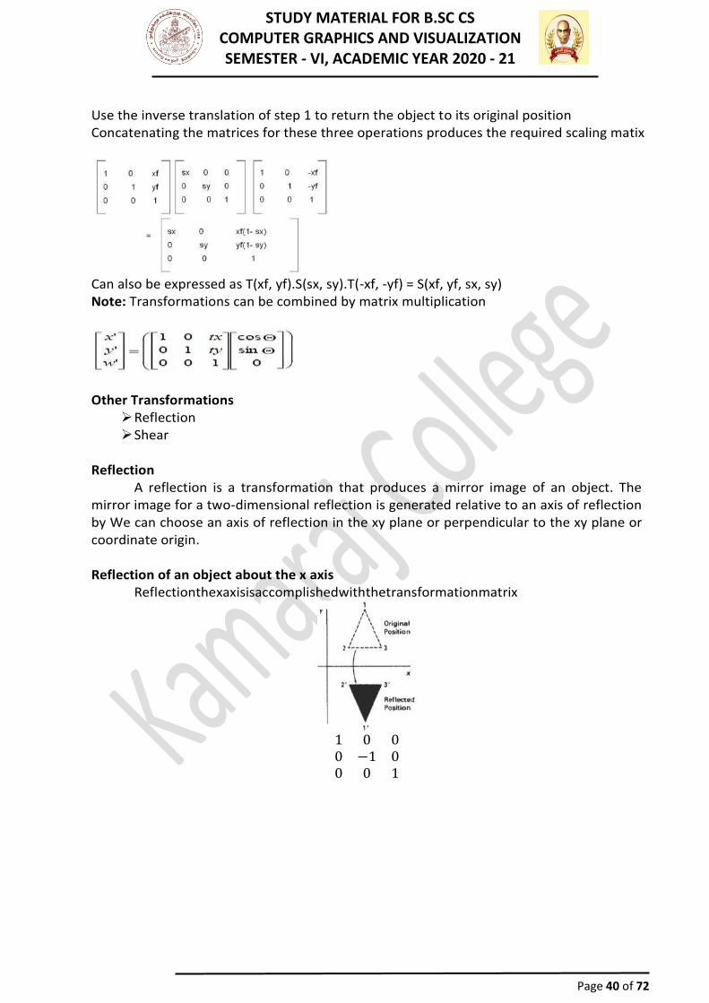
A reflection is a transformation that produces a mirror image of an object. The mirror image for a two-dimensional reflection is generated relative to an axis of reflection by We can choose an axis of reflection in the xy plane or perpendicular to the xy plane or coordinate origin. Reflection of an object about the x axis
Reflectionthexaxisisaccomplishedwiththetransformationmatrix
1 0 00 −1 00 0 1
STUDY MATERIAL FOR B.SC CS COMPUTER GRAPHICS AND VISUALIZATION SEMESTER - VI, ACADEMIC YEAR 2020 - 21
Page 41 of 72
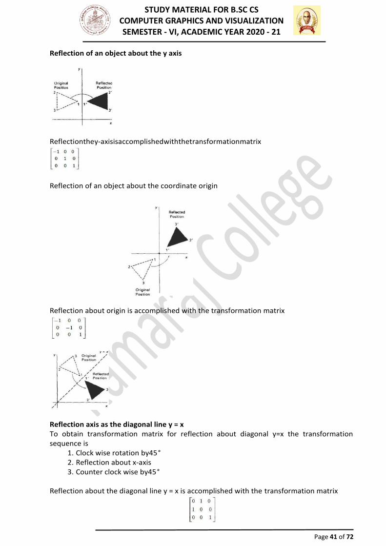
Reflection of an object about the y axis
Reflectionthey-axisisaccomplishedwiththetransformationmatrix
Reflection of an object about the coordinate origin
Reflection about origin is accomplished with the transformation matrix
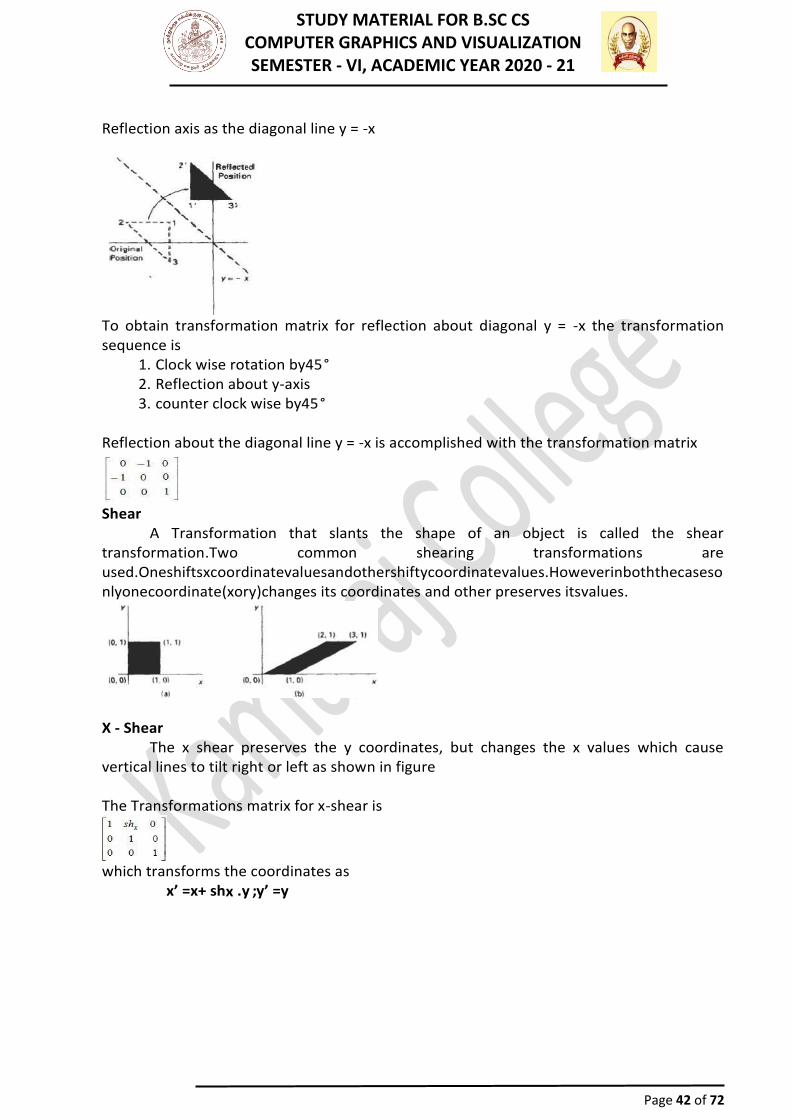
Reflection axis as the diagonal line y = x To obtain transformation matrix for reflection about diagonal y=x the transformation sequence is
1. Clock wise rotation by45° 2. Reflection about x-axis 3. Counter clock wise by45°
Reflection about the diagonal line y = x is accomplished with the transformation matrix
STUDY MATERIAL FOR B.SC CS COMPUTER GRAPHICS AND VISUALIZATION SEMESTER - VI, ACADEMIC YEAR 2020 - 21
Page 42 of 72
Reflection axis as the diagonal line y = -x
To obtain transformation matrix for reflection about diagonal y = -x the transformation sequence is
1. Clock wise rotation by45° 2. Reflection about y-axis 3. counter clock wise by45°
Reflection about the diagonal line y = -x is accomplished with the transformation matrix
Shear
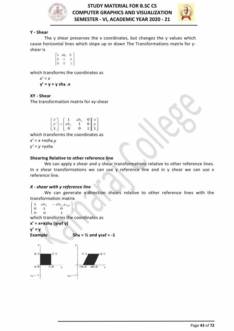
A Transformation that slants the shape of an object is called the shear transformation.Two common shearing transformations are used.Oneshiftsxcoordinatevaluesandothershiftycoordinatevalues.Howeverinboththecasesonlyonecoordinate(xory)changes its coordinates and other preserves itsvalues.
X - Shear
The x shear preserves the y coordinates, but changes the x values which cause vertical lines to tilt right or left as shown in figure The Transformations matrix for x-shear is
which transforms the coordinates as x’ =x+ shx .y ;y’ =y
STUDY MATERIAL FOR B.SC CS COMPUTER GRAPHICS AND VISUALIZATION SEMESTER - VI, ACADEMIC YEAR 2020 - 21
Page 43 of 72
Y - Shear The y shear preserves the x coordinates, but changes the y values which
cause horizontal lines which slope up or down The Transformations matrix for y-shear is which transforms the coordinates as
x’ = x y’ = y + y shx .x
XY - Shear The transformation matrix for xy-shear
which transforms the coordinates as x’ = x +xshx.y y’ = y +yshx
Shearing Relative to other reference line
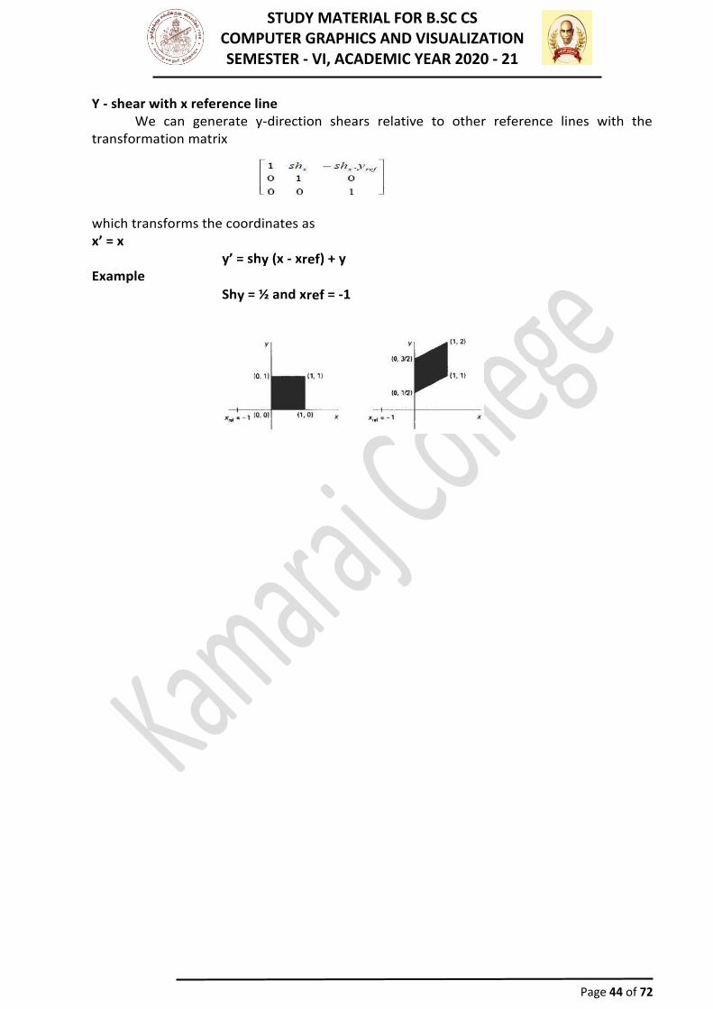
We can apply x shear and y shear transformations relative to other reference lines. In x shear transformations we can use y reference line and in y shear we can use x reference line. X - shear with y reference line
We can generate x-direction shears relative to other reference lines with the transformation matrix
which transforms the coordinates as x’ = x+xshx (yref y)
y’ = y Example Shx = ½ and yref = -1
STUDY MATERIAL FOR B.SC CS COMPUTER GRAPHICS AND VISUALIZATION SEMESTER - VI, ACADEMIC YEAR 2020 - 21
Page 44 of 72
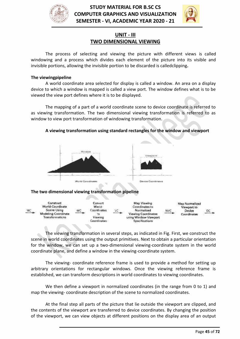
Y - shear with x reference line We can generate y-direction shears relative to other reference lines with the
transformation matrix
which transforms the coordinates as x’ = x Example
y’ = shy (x - xref) + y
Shy = ½ and xref = -1
STUDY MATERIAL FOR B.SC CS COMPUTER GRAPHICS AND VISUALIZATION SEMESTER - VI, ACADEMIC YEAR 2020 - 21
Page 45 of 72
UNIT - III TWO DIMENSIONAL VIEWING
The process of selecting and viewing the picture with different views is called
windowing and a process which divides each element of the picture into its visible and invisible portions, allowing the invisible portion to be discarded is calledclipping.
The viewingpipeline
A world coordinate area selected for display is called a window. An area on a display device to which a window is mapped is called a view port. The window defines what is to be viewed the view port defines where it is to be displayed.
The mapping of a part of a world coordinate scene to device coordinate is referred to as viewing transformation. The two dimensional viewing transformation is referred to as window to view port transformation of windowing transformation.
A viewing transformation using standard rectangles for the window and viewport
The two dimensional viewing transformation pipeline
The viewing transformation in several steps, as indicated in Fig. First, we construct the
scene in world coordinates using the output primitives. Next to obtain a particular orientation for the window, we can set up a two-dimensional viewing-coordinate system in the world coordinate plane, and define a window in the viewing-coordinate system.
The viewing- coordinate reference frame is used to provide a method for setting up arbitrary orientations for rectangular windows. Once the viewing reference frame is established, we can transform descriptions in world coordinates to viewing coordinates.
We then define a viewport in normalized coordinates (in the range from 0 to 1) and map the viewing- coordinate description of the scene to normalized coordinates.
At the final step all parts of the picture that lie outside the viewport are clipped, and the contents of the viewport are transferred to device coordinates. By changing the position of the viewport, we can view objects at different positions on the display area of an output
STUDY MATERIAL FOR B.SC CS COMPUTER GRAPHICS AND VISUALIZATION SEMESTER - VI, ACADEMIC YEAR 2020 - 21
Page 46 of 72
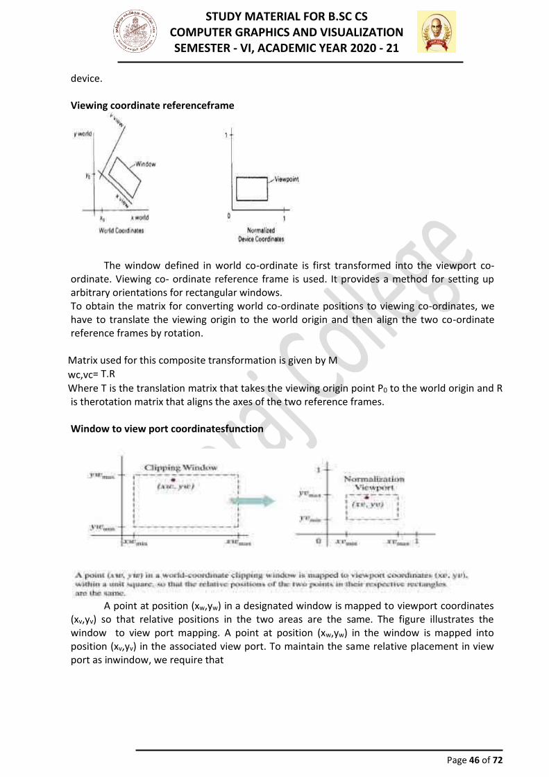
device. Viewing coordinate referenceframe
The window defined in world co-ordinate is first transformed into the viewport co-ordinate. Viewing co- ordinate reference frame is used. It provides a method for setting up arbitrary orientations for rectangular windows. To obtain the matrix for converting world co-ordinate positions to viewing co-ordinates, we have to translate the viewing origin to the world origin and then align the two co-ordinate reference frames by rotation.
Matrix used for this composite transformation is given by M
wc,vc= T.R
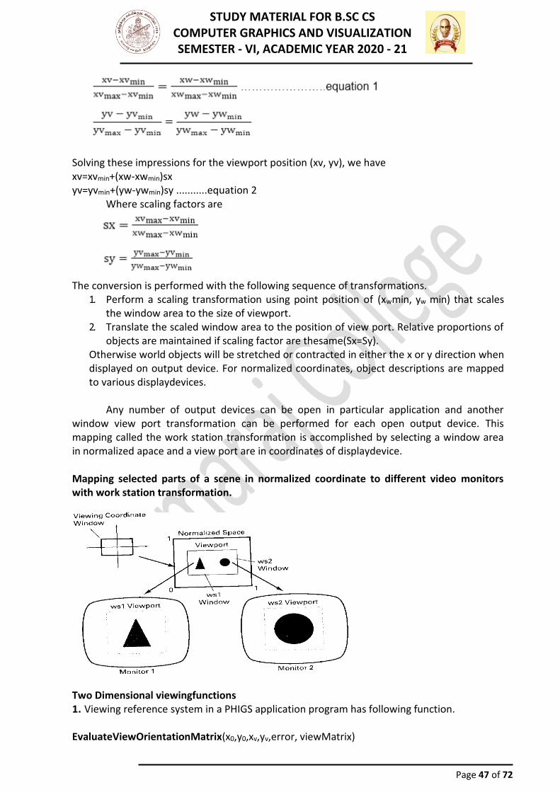
Where T is the translation matrix that takes the viewing origin point P0 to the world origin and R is therotation matrix that aligns the axes of the two reference frames. Window to view port coordinatesfunction
A point at position (xw,yw) in a designated window is mapped to viewport coordinates
(xv,yv) so that relative positions in the two areas are the same. The figure illustrates the window to view port mapping. A point at position (xw,yw) in the window is mapped into position (xv,yv) in the associated view port. To maintain the same relative placement in view port as inwindow, we require that
STUDY MATERIAL FOR B.SC CS COMPUTER GRAPHICS AND VISUALIZATION SEMESTER - VI, ACADEMIC YEAR 2020 - 21
Page 47 of 72
Solving these impressions for the viewport position (xv, yv), we have xv=xvmin+(xw-xwmin)sx yv=yvmin+(yw-ywmin)sy ...........equation 2
Where scaling factors are
The conversion is performed with the following sequence of transformations.
1. Perform a scaling transformation using point position of (xwmin, yw min) that scales the window area to the size of viewport.
2. Translate the scaled window area to the position of view port. Relative proportions of objects are maintained if scaling factor are thesame(Sx=Sy).
Otherwise world objects will be stretched or contracted in either the x or y direction when displayed on output device. For normalized coordinates, object descriptions are mapped to various displaydevices.
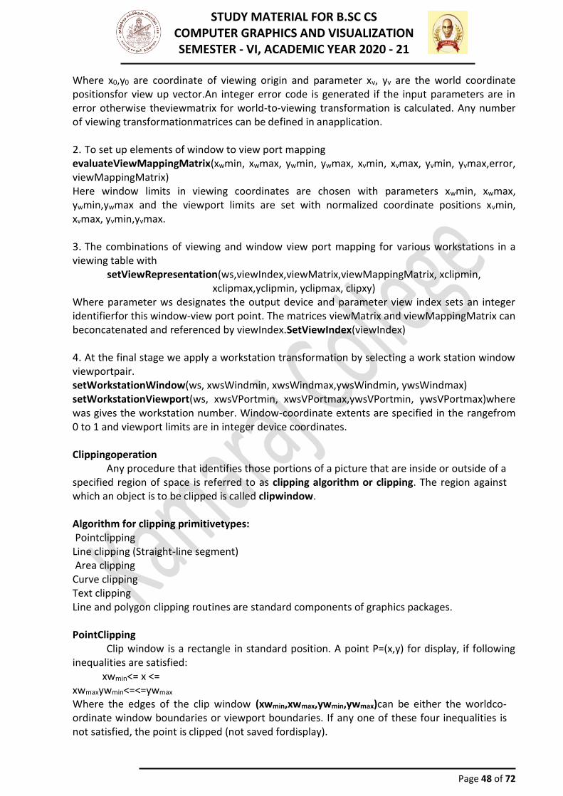
Any number of output devices can be open in particular application and another
window view port transformation can be performed for each open output device. This mapping called the work station transformation is accomplished by selecting a window area in normalized apace and a view port are in coordinates of displaydevice.
Mapping selected parts of a scene in normalized coordinate to different video monitors with work station transformation.
Two Dimensional viewingfunctions 1. Viewing reference system in a PHIGS application program has following function.
EvaluateViewOrientationMatrix(x0,y0,xv,yv,error, viewMatrix)
STUDY MATERIAL FOR B.SC CS COMPUTER GRAPHICS AND VISUALIZATION SEMESTER - VI, ACADEMIC YEAR 2020 - 21
Page 48 of 72
Where x0,y0 are coordinate of viewing origin and parameter xv, yv are the world coordinate positionsfor view up vector.An integer error code is generated if the input parameters are in error otherwise theviewmatrix for world-to-viewing transformation is calculated. Any number of viewing transformationmatrices can be defined in anapplication. 2. To set up elements of window to view port mapping evaluateViewMappingMatrix(xwmin, xwmax, ywmin, ywmax, xvmin, xvmax, yvmin, yvmax,error, viewMappingMatrix) Here window limits in viewing coordinates are chosen with parameters xwmin, xwmax, ywmin,ywmax and the viewport limits are set with normalized coordinate positions xvmin, xvmax, yvmin,yvmax. 3. The combinations of viewing and window view port mapping for various workstations in a viewing table with
setViewRepresentation(ws,viewIndex,viewMatrix,viewMappingMatrix, xclipmin, xclipmax,yclipmin, yclipmax, clipxy)
Where parameter ws designates the output device and parameter view index sets an integer identifierfor this window-view port point. The matrices viewMatrix and viewMappingMatrix can beconcatenated and referenced by viewIndex.SetViewIndex(viewIndex) 4. At the final stage we apply a workstation transformation by selecting a work station window viewportpair. setWorkstationWindow(ws, xwsWindmin, xwsWindmax,ywsWindmin, ywsWindmax) setWorkstationViewport(ws, xwsVPortmin, xwsVPortmax,ywsVPortmin, ywsVPortmax)where was gives the workstation number. Window-coordinate extents are specified in the rangefrom 0 to 1 and viewport limits are in integer device coordinates. Clippingoperation
Any procedure that identifies those portions of a picture that are inside or outside of a specified region of space is referred to as clipping algorithm or clipping. The region against which an object is to be clipped is called clipwindow. Algorithm for clipping primitivetypes: Pointclipping Line clipping (Straight-line segment) Area clipping Curve clipping Text clipping Line and polygon clipping routines are standard components of graphics packages. PointClipping
Clip window is a rectangle in standard position. A point P=(x,y) for display, if following inequalities are satisfied:
xwmin<= x <= xwmaxywmin<=<=ywmax Where the edges of the clip window (xwmin,xwmax,ywmin,ywmax)can be either the worldco-ordinate window boundaries or viewport boundaries. If any one of these four inequalities is not satisfied, the point is clipped (not saved fordisplay).
STUDY MATERIAL FOR B.SC CS COMPUTER GRAPHICS AND VISUALIZATION SEMESTER - VI, ACADEMIC YEAR 2020 - 21
Page 49 of 72
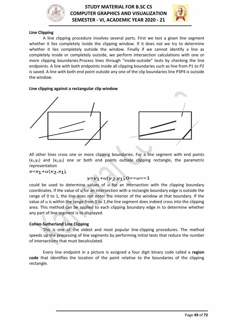
Line Clipping A line clipping procedure involves several parts. First we test a given line segment
whether it lies completely inside the clipping window. If it does not we try to determine whether it lies completely outside the window. Finally if we cannot identify a line as completely inside or completely outside, we perform intersection calculations with one or more clipping boundaries.Process lines through “inside-outside” tests by checking the line endpoints. A line with both endpoints inside all clipping boundaries such as line from P1 to P2 is saved. A line with both end point outside any one of the clip boundaries line P3P4 is outside the window.
Line clipping against a rectangular clip window
All other lines cross one or more clipping boundaries. For a line segment with end points (x1,y1) and (x2,y2) one or both end points outside clipping rectangle, the parametric representation x=x1+u(x2-x1),
y=y1+u(y2-y1),0<=u<=1
could be used to determine values of u for an intersection with the clipping boundary coordinates. If the value of u for an intersection with a rectangle boundary edge is outside the range of 0 to 1, the line does not enter the interior of the window at that boundary. If the value of u is within the range from 0 to 1,the line segment does indeed cross into the clipping area. This method can be applied to each clipping boundary edge in to determine whether any part of line segment is to displayed. Cohen-Sutherland Line Clipping
This is one of the oldest and most popular line-clipping procedures. The method speeds up the processing of line segments by performing initial tests that reduce the number of intersections that must becalculated.
Every line endpoint in a picture is assigned a four digit binary code called a region code that identifies the location of the point relative to the boundaries of the clipping rectangle.
STUDY MATERIAL FOR B.SC CS COMPUTER GRAPHICS AND VISUALIZATION SEMESTER - VI, ACADEMIC YEAR 2020 - 21
Page 50 of 72
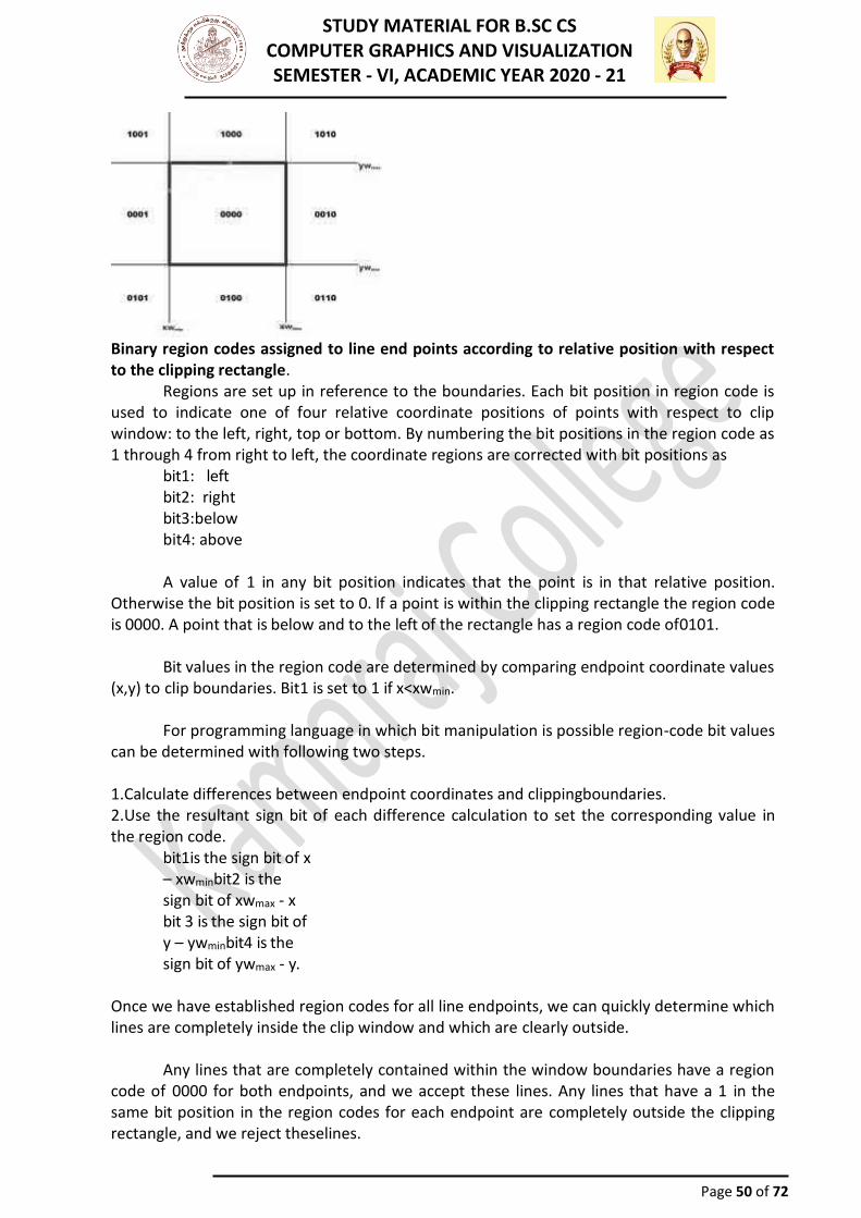
Binary region codes assigned to line end points according to relative position with respect to the clipping rectangle.
Regions are set up in reference to the boundaries. Each bit position in region code is used to indicate one of four relative coordinate positions of points with respect to clip window: to the left, right, top or bottom. By numbering the bit positions in the region code as 1 through 4 from right to left, the coordinate regions are corrected with bit positions as
bit1: left bit2: right bit3:below bit4: above
A value of 1 in any bit position indicates that the point is in that relative position.
Otherwise the bit position is set to 0. If a point is within the clipping rectangle the region code is 0000. A point that is below and to the left of the rectangle has a region code of0101.
Bit values in the region code are determined by comparing endpoint coordinate values (x,y) to clip boundaries. Bit1 is set to 1 if x<xwmin.
For programming language in which bit manipulation is possible region-code bit values can be determined with following two steps. 1.Calculate differences between endpoint coordinates and clippingboundaries. 2.Use the resultant sign bit of each difference calculation to set the corresponding value in the region code.
bit1is the sign bit of x – xwminbit2 is the sign bit of xwmax - x bit 3 is the sign bit of y – ywminbit4 is the sign bit of ywmax - y.
Once we have established region codes for all line endpoints, we can quickly determine which lines are completely inside the clip window and which are clearly outside.
Any lines that are completely contained within the window boundaries have a region
code of 0000 for both endpoints, and we accept these lines. Any lines that have a 1 in the same bit position in the region codes for each endpoint are completely outside the clipping rectangle, and we reject theselines.
STUDY MATERIAL FOR B.SC CS COMPUTER GRAPHICS AND VISUALIZATION SEMESTER - VI, ACADEMIC YEAR 2020 - 21
Page 51 of 72
We would discard the line that has a region code of 1001 for one endpoint and a code
of 0101 for the other endpoint. Both endpoints of this line are left of the clipping rectangle, as indicated by the 1 in the first bit position of each regioncode.
A method that can be used to test lines for total clipping is to perform the logical and
operation with both region codes. If the result is not 0000,the line is completely outside the clipping region.
Lines that cannot be identified as completely inside or completely outside a clip
window by these tests are checked for intersection with window boundaries.
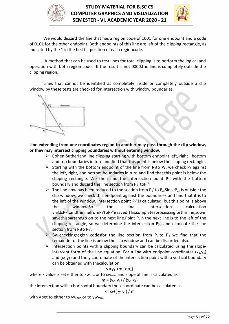
Line extending from one coordinates region to another may pass through the clip window, or they may intersect clipping boundaries without entering window.
➢ Cohen-Sutherland line clipping starting with bottom endpoint left, right , bottom and top boundaries in turn and find that this point is below the clipping rectangle.
➢ Starting with the bottom endpoint of the line from P1to P2, we check P1 against the left, right, and bottom boundaries in turn and find that this point is below the clipping rectangle. We then find the intersection point P1‟ with the bottom boundary and discard the line section from P1 toP1‟.
➢ The line now has been reduced to the section from P1‟ to P2,SinceP2, is outside the clip window, we check this endpoint against the boundaries and find that it is to the left of the window. Intersection point P2‟ is calculated, but this point is above the window.So the final intersection calculation yieldsP2”,andthelinefromP1‟toP2”issaved.Thiscompletesprocessingforthisline,sowesavethispartandgo on to the next line.Point P3in the next line is to the left of the clipping rectangle, so we determine the intersection P3‟, and eliminate the line section from P3to P3'.
➢ By checkingregion codesfor the line section from P3'to P4 we find that the remainder of the line is below the clip window and can be discarded also.
➢ Intersection points with a clipping boundary can be calculated using the slope-intercept form of the line equation. For a line with endpoint coordinates (x1,y1) and (x2,y2) and the y coordinate of the intersection point with a vertical boundary can be obtained with thecalculation.
y =y1 +m (x-x1) where x value is set either to xwmin or to xwmax and slope of line is calculated as
m = (y2- y1) / (x2- x1) the intersection with a horizontal boundary the x coordinate can be calculated as
x= x1+( y- y1) / m with y set to either to ywmin or to ywmax.
STUDY MATERIAL FOR B.SC CS COMPUTER GRAPHICS AND VISUALIZATION SEMESTER - VI, ACADEMIC YEAR 2020 - 21
Page 52 of 72
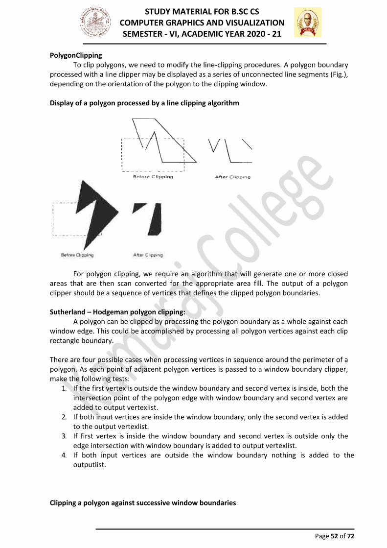
PolygonClipping To clip polygons, we need to modify the line-clipping procedures. A polygon boundary
processed with a line clipper may be displayed as a series of unconnected line segments (Fig.), depending on the orientation of the polygon to the clipping window. Display of a polygon processed by a line clipping algorithm
For polygon clipping, we require an algorithm that will generate one or more closed areas that are then scan converted for the appropriate area fill. The output of a polygon clipper should be a sequence of vertices that defines the clipped polygon boundaries.
Sutherland – Hodgeman polygon clipping:
A polygon can be clipped by processing the polygon boundary as a whole against each window edge. This could be accomplished by processing all polygon vertices against each clip rectangle boundary. There are four possible cases when processing vertices in sequence around the perimeter of a polygon. As each point of adjacent polygon vertices is passed to a window boundary clipper, make the following tests:
1. If the first vertex is outside the window boundary and second vertex is inside, both the intersection point of the polygon edge with window boundary and second vertex are added to output vertexlist.
2. If both input vertices are inside the window boundary, only the second vertex is added to the output vertexlist.
3. If first vertex is inside the window boundary and second vertex is outside only the edge intersection with window boundary is added to output vertexlist.
4. If both input vertices are outside the window boundary nothing is added to the outputlist.
Clipping a polygon against successive window boundaries
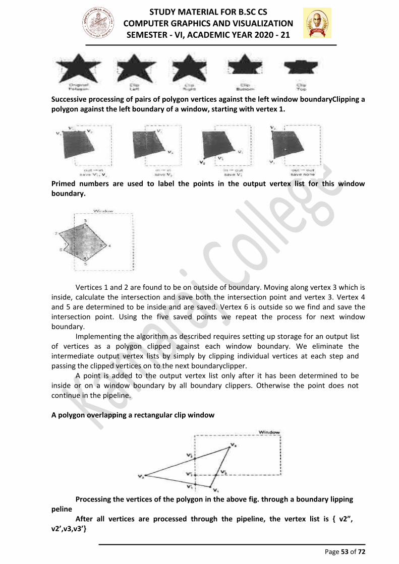
STUDY MATERIAL FOR B.SC CS COMPUTER GRAPHICS AND VISUALIZATION SEMESTER - VI, ACADEMIC YEAR 2020 - 21
Page 53 of 72
Successive processing of pairs of polygon vertices against the left window boundaryClipping a polygon against the left boundary of a window, starting with vertex 1.
Primed numbers are used to label the points in the output vertex list for this window boundary.
Vertices 1 and 2 are found to be on outside of boundary. Moving along vertex 3 which is inside, calculate the intersection and save both the intersection point and vertex 3. Vertex 4 and 5 are determined to be inside and are saved. Vertex 6 is outside so we find and save the intersection point. Using the five saved points we repeat the process for next window boundary.
Implementing the algorithm as described requires setting up storage for an output list of vertices as a polygon clipped against each window boundary. We eliminate the intermediate output vertex lists by simply by clipping individual vertices at each step and passing the clipped vertices on to the next boundaryclipper.
A point is added to the output vertex list only after it has been determined to be inside or on a window boundary by all boundary clippers. Otherwise the point does not continue in the pipeline. A polygon overlapping a rectangular clip window
Processing the vertices of the polygon in the above fig. through a boundary lipping
peline After all vertices are processed through the pipeline, the vertex list is { v2”,
v2’,v3,v3’}
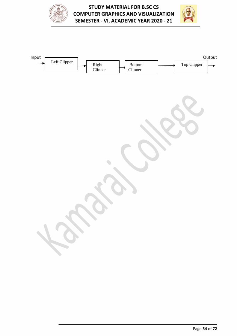
STUDY MATERIAL FOR B.SC CS COMPUTER GRAPHICS AND VISUALIZATION SEMESTER - VI, ACADEMIC YEAR 2020 - 21
Page 54 of 72
Input Output Output
Left Clipper Right
Clipper
Bottom
Clipper
Top Clipper
STUDY MATERIAL FOR B.SC CS COMPUTER GRAPHICS AND VISUALIZATION SEMESTER - VI, ACADEMIC YEAR 2020 - 21
Page 55 of 72
UNIT - IV GRAPHICAL USER INTERFACES AND INTERACTIVE INPUT METHODS
In order to be able to interact with the graphical image input methods are required.
These can be used to just change the location and orientation of the camera, or to change specific settings of the rendering itself.
Different devices are more suitable for changing some settings then others. In this chapter we will specify different types of these devices and discuss their advantages. Input methods can be classified using the following categories:
➢ Locator ➢ Stroke ➢ String ➢ Valuator ➢ Choice ➢ Pick
Locator
A device that allows the user to specify one co-ordinate position. Different methods can be used, such as a mouse cursor, where a location is chosen by clicking a button, or a cursor that is moved using different keys on the keyboard. Touch screens can also be used as locators; the user specifies the location by inducing force onto the desired coordinate on the screen. Stroke
A device that allows the user to specify a set of coordinate positions. The positions can be specified, for example, by dragging the mouse across the screen while a mouse button is kept pressed. On release, a second coordinate can be used to define a rectangular area using the first coordinate inaddition. String
A device that allows the user to specify text input. A text input widget in combination with the keyboard is used to input the text. Also, virtual keyboards displayed on the screen where the characters can be picked using the mouse can be used if keyboards are not available to the application. Valuator
A device that allows the user to specify a scalar value. Similar to string inputs, numeric values can be specified using the keyboard. Often, up-down-arrows are added to increase or decrease the current value. Rotary devices, such as wheels can also be used for specifying numerical values. Often times, it is useful to limit the range of the numerical value depending on the value. Choice
A device that allows the user to specify a menu option. Typical choice devices are menus or radio buttons which provide various options the user can choose from. For radio buttons, often only one option can be chosen at a time. Once another option is picked, the previous one gets cleared. Pick
STUDY MATERIAL FOR B.SC CS COMPUTER GRAPHICS AND VISUALIZATION SEMESTER - VI, ACADEMIC YEAR 2020 - 21
Page 56 of 72
A device that allows the user to specify a component of a picture. Similar to locator devices, a coordinateis specified using the mouse or other cursor input devices and then back-projected into the scene to determine the selected 3-D object. It is often useful to allow a certain “error tolerance” so that an object is picked even though the user did not exactly onto the object but close enough next to it. Also, highlighting objects within the scene can be used to traverse through a list of objects that fulfill the proximity criterion. INPUT FUNCTIONS Input Modes
➢ Specify how the program and input device shouldinteract including request mode, sample mode and eventmode
Request Mode
➢ the application program initiate data entry Sample Mode
➢ the application program and input devices operate independently Event Mode
➢ the input device initiate data input to the application program Other functions are used to specify physical devicesfor the logical dataclasses
THREE DIMENSIONAL DISPLAY METHODS
To obtain display of a three-dimensional scene that has been modeled in world coordinates. We must first set up a coordinate reference for the "camera". This coordinate reference defines the position and orientation for the plane of the camera film which is the plane we want to us to display a view of the objects in the scene. Object descriptions are then transferred to the camera reference coordinates and projected onto the selected display plane. We can then display the objects in wireframe (outline) form, or we can apply lighting surface rendering techniques to shade the visible surfaces. Parallel Projection
In a parallel projection, parallel lines in the world-coordinate scene projected into parallel lines on the two-dimensional display plane. Perspective Projection
Another method for generating a view of a three-dimensional scene is to project points to the display plane along converging paths. This causes objects farther from the viewing position to be displayed smaller than objects of the same size that are nearer to the viewing position.In a perspective projection, parallel lines in a scene that are not parallel to the display plane are projected into converging lines Depth Cueing
A simple method for indicating depth with wireframe displays is to vary the intensity of objects according to their distance from the viewing position. The viewing position are displayed with the highest intensities, and lines farther away are displayed with decreasing intensities. Visible Line and Surface Identification
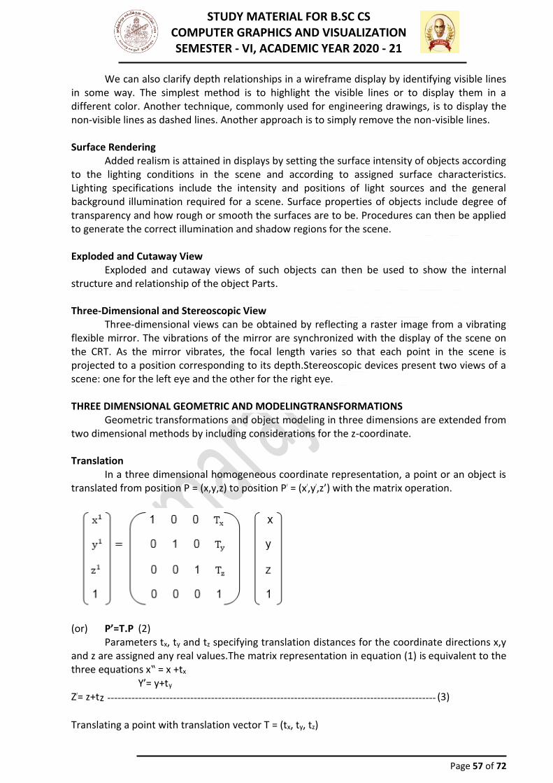
STUDY MATERIAL FOR B.SC CS COMPUTER GRAPHICS AND VISUALIZATION SEMESTER - VI, ACADEMIC YEAR 2020 - 21
Page 57 of 72
We can also clarify depth relationships in a wireframe display by identifying visible lines in some way. The simplest method is to highlight the visible lines or to display them in a different color. Another technique, commonly used for engineering drawings, is to display the non-visible lines as dashed lines. Another approach is to simply remove the non-visible lines. Surface Rendering
Added realism is attained in displays by setting the surface intensity of objects according to the lighting conditions in the scene and according to assigned surface characteristics. Lighting specifications include the intensity and positions of light sources and the general background illumination required for a scene. Surface properties of objects include degree of transparency and how rough or smooth the surfaces are to be. Procedures can then be applied to generate the correct illumination and shadow regions for the scene. Exploded and Cutaway View
Exploded and cutaway views of such objects can then be used to show the internal structure and relationship of the object Parts. Three-Dimensional and Stereoscopic View
Three-dimensional views can be obtained by reflecting a raster image from a vibrating flexible mirror. The vibrations of the mirror are synchronized with the display of the scene on the CRT. As the mirror vibrates, the focal length varies so that each point in the scene is projected to a position corresponding to its depth.Stereoscopic devices present two views of a scene: one for the left eye and the other for the right eye. THREE DIMENSIONAL GEOMETRIC AND MODELINGTRANSFORMATIONS
Geometric transformations and object modeling in three dimensions are extended from two dimensional methods by including considerations for the z-coordinate. Translation
In a three dimensional homogeneous coordinate representation, a point or an object is translated from position P = (x,y,z) to position P’ = (x’,y’,z’) with the matrix operation.
(or) P’=T.P (2)
Parameters tx, ty and tz specifying translation distances for the coordinate directions x,y and z are assigned any real values.The matrix representation in equation (1) is equivalent to the three equations x‟ = x +tx
Y’= y+ty Z’= z+tz ----------------------------------------------------------------------------------------------- (3)
Translating a point with translation vector T = (tx, ty, tz)
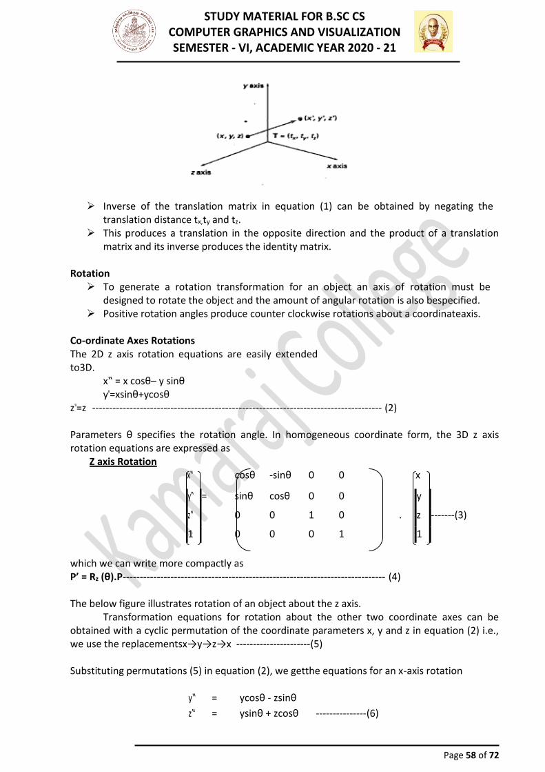
STUDY MATERIAL FOR B.SC CS COMPUTER GRAPHICS AND VISUALIZATION SEMESTER - VI, ACADEMIC YEAR 2020 - 21
Page 58 of 72
➢ Inverse of the translation matrix in equation (1) can be obtained by negating the
translation distance tx,ty and tz. ➢ This produces a translation in the opposite direction and the product of a translation
matrix and its inverse produces the identity matrix. Rotation
➢ To generate a rotation transformation for an object an axis of rotation must be designed to rotate the object and the amount of angular rotation is also bespecified.
➢ Positive rotation angles produce counter clockwise rotations about a coordinateaxis. Co-ordinate Axes Rotations The 2D z axis rotation equations are easily extended to3D.
x‟ = x cosθ– y sinθ y‟=xsinθ+ycosθ
z‟=z ------------------------------------------------------------------------------------- (2) Parameters θ specifies the rotation angle. In homogeneous coordinate form, the 3D z axis rotation equations are expressed as
Z axis Rotation x‟
cosθ
-sinθ
0
0
x
y‟ = sinθ cosθ 0 0 y
z‟ 0 0 1 0 . z -------(3)
1 0 0 0 1 1
which we can write more compactly as P’ = Rz (θ).P ----------------------------------------------------------------------------- (4) The below figure illustrates rotation of an object about the z axis.
Transformation equations for rotation about the other two coordinate axes can be obtained with a cyclic permutation of the coordinate parameters x, y and z in equation (2) i.e., we use the replacementsx→y→z→x ----------------------(5) Substituting permutations (5) in equation (2), we getthe equations for an x-axis rotation
y‟ = ycosθ - zsinθ
z‟ = ysinθ + zcosθ ---------------(6)
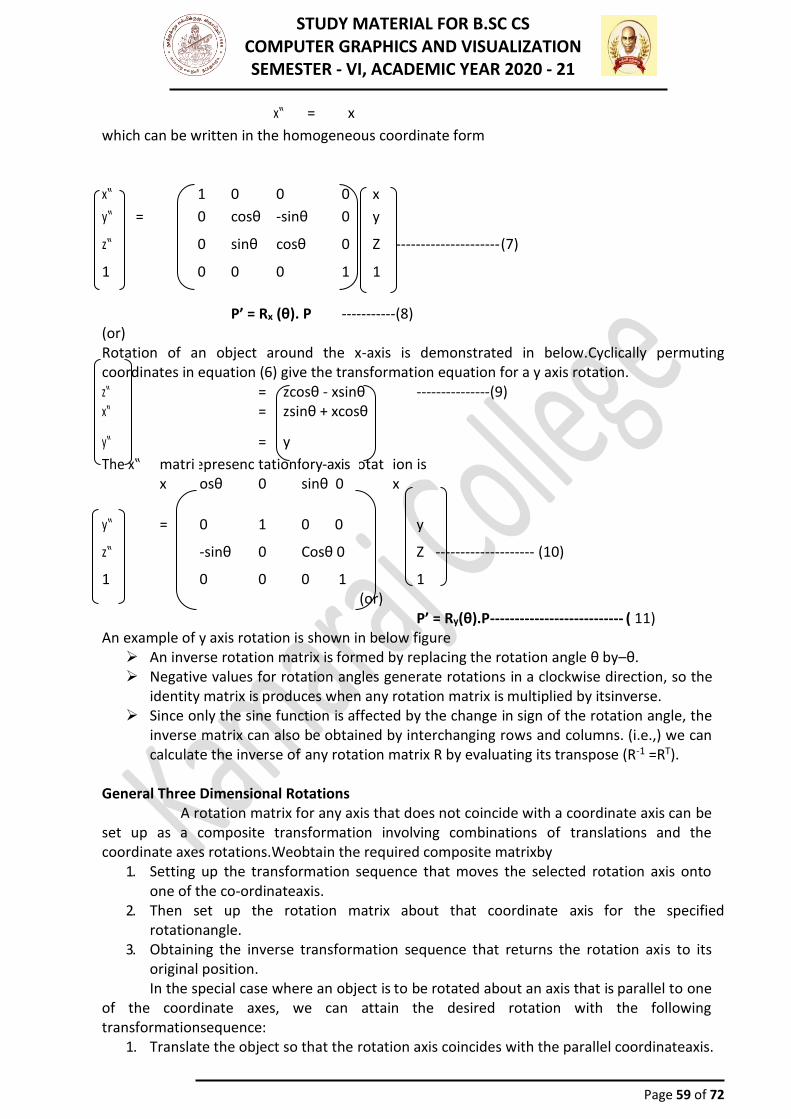
STUDY MATERIAL FOR B.SC CS COMPUTER GRAPHICS AND VISUALIZATION SEMESTER - VI, ACADEMIC YEAR 2020 - 21
Page 59 of 72
x‟ = x
which can be written in the homogeneous coordinate form
Rotation of an object around the x-axis is demonstrated in below.Cyclically permuting coordinates in equation (6) give the transformation equation for a y axis rotation.
An example of y axis rotation is shown in below figure ➢ An inverse rotation matrix is formed by replacing the rotation angle θ by–θ. ➢ Negative values for rotation angles generate rotations in a clockwise direction, so the
identity matrix is produces when any rotation matrix is multiplied by itsinverse. ➢ Since only the sine function is affected by the change in sign of the rotation angle, the
inverse matrix can also be obtained by interchanging rows and columns. (i.e.,) we can calculate the inverse of any rotation matrix R by evaluating its transpose (R-1 =RT).
General Three Dimensional Rotations A rotation matrix for any axis that does not coincide with a coordinate axis can be set up as a composite transformation involving combinations of translations and the coordinate axes rotations.Weobtain the required composite matrixby
1. Setting up the transformation sequence that moves the selected rotation axis onto one of the co-ordinateaxis.
2. Then set up the rotation matrix about that coordinate axis for the specified rotationangle.
3. Obtaining the inverse transformation sequence that returns the rotation axis to its original position. In the special case where an object is to be rotated about an axis that is parallel to one
of the coordinate axes, we can attain the desired rotation with the following transformationsequence:
1. Translate the object so that the rotation axis coincides with the parallel coordinateaxis.
x‟ 1 0 0 0 x
y‟ = 0 cosθ -sinθ 0 y
z‟ 0 sinθ cosθ 0 Z --------------------- (7)
1 0 0 0 1 1
(or)
P’ = Rx (θ). P
-----------(8)
z‟ x‟
= =
zcosθ - xsinθ zsinθ + xcosθ
---------------(9)
y‟ = y
The x‟ matrix
represencosθ
tationf 0
ory-axis sinθ 0
rotat 0
ion is x
y‟ = 0 1 0 0 y
z‟ -sinθ 0 Cosθ 0 Z -------------------- (10)
1 0 0 0 1 (or)
1 P’ = Ry(θ).P --------------------------- ( 11)
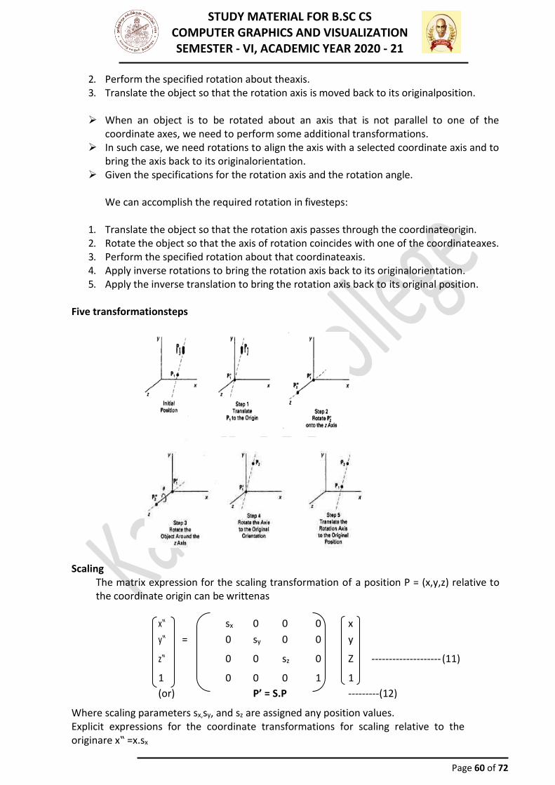
STUDY MATERIAL FOR B.SC CS COMPUTER GRAPHICS AND VISUALIZATION SEMESTER - VI, ACADEMIC YEAR 2020 - 21
Page 60 of 72
2. Perform the specified rotation about theaxis. 3. Translate the object so that the rotation axis is moved back to its originalposition.
➢ When an object is to be rotated about an axis that is not parallel to one of the
coordinate axes, we need to perform some additional transformations. ➢ In such case, we need rotations to align the axis with a selected coordinate axis and to
bring the axis back to its originalorientation. ➢ Given the specifications for the rotation axis and the rotation angle.
We can accomplish the required rotation in fivesteps:
1. Translate the object so that the rotation axis passes through the coordinateorigin. 2. Rotate the object so that the axis of rotation coincides with one of the coordinateaxes. 3. Perform the specified rotation about that coordinateaxis. 4. Apply inverse rotations to bring the rotation axis back to its originalorientation. 5. Apply the inverse translation to bring the rotation axis back to its original position.
Five transformationsteps
Scaling
The matrix expression for the scaling transformation of a position P = (x,y,z) relative to the coordinate origin can be writtenas
x‟ sx 0 0 0 x
y‟ = 0 sy 0 0 y
z‟ 0 0 sz 0 Z -------------------- (11)
1 0 0 0 1 1
(or) P’ = S.P ---------(12)
Where scaling parameters sx,sy, and sz are assigned any position values. ➢ Explicit expressions for the coordinate transformations for scaling relative to the
originare x‟ =x.sx
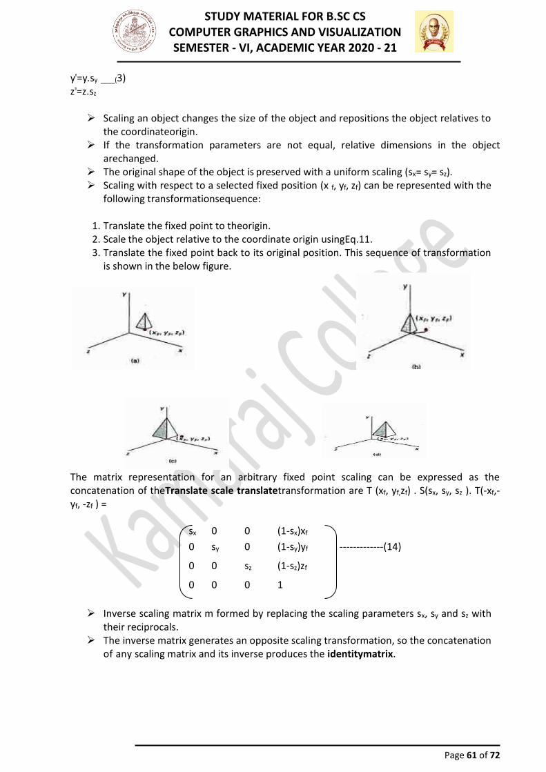
STUDY MATERIAL FOR B.SC CS COMPUTER GRAPHICS AND VISUALIZATION SEMESTER - VI, ACADEMIC YEAR 2020 - 21
Page 61 of 72
y‟=y.sy ____(3) z‟=z.sz
➢ Scaling an object changes the size of the object and repositions the object relatives to
the coordinateorigin. ➢ If the transformation parameters are not equal, relative dimensions in the object
arechanged. ➢ The original shape of the object is preserved with a uniform scaling (sx= sy= sz). ➢ Scaling with respect to a selected fixed position (x f, yf, zf) can be represented with the
following transformationsequence:
1. Translate the fixed point to theorigin. 2. Scale the object relative to the coordinate origin usingEq.11. 3. Translate the fixed point back to its original position. This sequence of transformation
is shown in the below figure.
The matrix representation for an arbitrary fixed point scaling can be expressed as the concatenation of theTranslate scale translatetransformation are T (xf, yf,zf) . S(sx, sy, sz ). T(-xf,-yf, -zf ) =
sx 0 0 (1-sx)xf
0 sy 0 (1-sy)yf -------------(14)
0 0 sz (1-sz)zf
0 0 0 1
➢ Inverse scaling matrix m formed by replacing the scaling parameters sx, sy and sz with
their reciprocals. ➢ The inverse matrix generates an opposite scaling transformation, so the concatenation
of any scaling matrix and its inverse produces the identitymatrix.
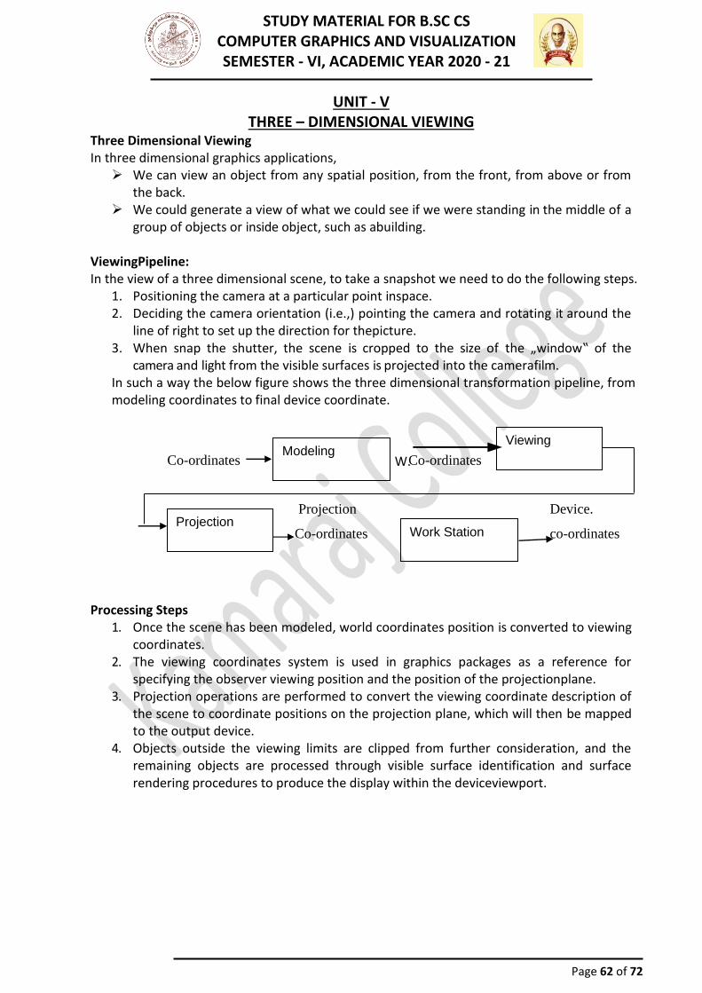
STUDY MATERIAL FOR B.SC CS COMPUTER GRAPHICS AND VISUALIZATION SEMESTER - VI, ACADEMIC YEAR 2020 - 21
Page 62 of 72
Co-ordinates Co-ordinates
Projection
Co-ordinates
Device.
co-ordinates
Viewing
Work Station Projection
Modeling
UNIT - V THREE – DIMENSIONAL VIEWING
Three Dimensional Viewing In three dimensional graphics applications,
➢ We can view an object from any spatial position, from the front, from above or from the back.
➢ We could generate a view of what we could see if we were standing in the middle of a group of objects or inside object, such as abuilding.
ViewingPipeline: In the view of a three dimensional scene, to take a snapshot we need to do the following steps.
1. Positioning the camera at a particular point inspace. 2. Deciding the camera orientation (i.e.,) pointing the camera and rotating it around the
line of right to set up the direction for thepicture. 3. When snap the shutter, the scene is cropped to the size of the „window‟ of the
camera and light from the visible surfaces is projected into the camerafilm. In such a way the below figure shows the three dimensional transformation pipeline, from modeling coordinates to final device coordinate.
W.
Processing Steps
1. Once the scene has been modeled, world coordinates position is converted to viewing coordinates.
2. The viewing coordinates system is used in graphics packages as a reference for specifying the observer viewing position and the position of the projectionplane.
3. Projection operations are performed to convert the viewing coordinate description of the scene to coordinate positions on the projection plane, which will then be mapped to the output device.
4. Objects outside the viewing limits are clipped from further consideration, and the remaining objects are processed through visible surface identification and surface rendering procedures to produce the display within the deviceviewport.
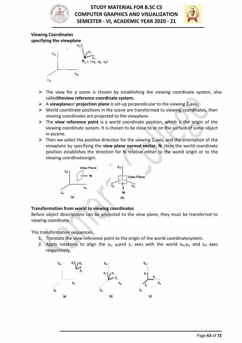
STUDY MATERIAL FOR B.SC CS COMPUTER GRAPHICS AND VISUALIZATION SEMESTER - VI, ACADEMIC YEAR 2020 - 21
Page 63 of 72
Viewing Coordinates specifying the viewplane
➢ The view for a scene is chosen by establishing the viewing coordinate system, also calledtheview reference coordinate system.
➢ A viewplaneor projection plane is set-up perpendicular to the viewing Zvaxis. ➢ World coordinate positions in the scene are transformed to viewing coordinates, then
viewing coordinates are projected to the viewplane. ➢ The view reference point is a world coordinate position, which is the origin of the
viewing coordinate system. It is chosen to be close to or on the surface of some object in ascene.
➢ Then we select the positive direction for the viewing Zvaxis, and the orientation of the viewplane by specifying the view plane normal vector, N. Here the world coordinate position establishes the direction for N relative either to the world origin or to the viewing coordinateorigin.
Transformation from world to viewing coordinates Before object descriptions can be projected to the view plane, they must be transferred to viewing coordinate. This transformation sequenceis,
1. Translate the view reference point to the origin of the world coordinatesystem. 2. Apply rotations to align the xv, yvand zv axes with the world xw,yw and zw axes
respectively.
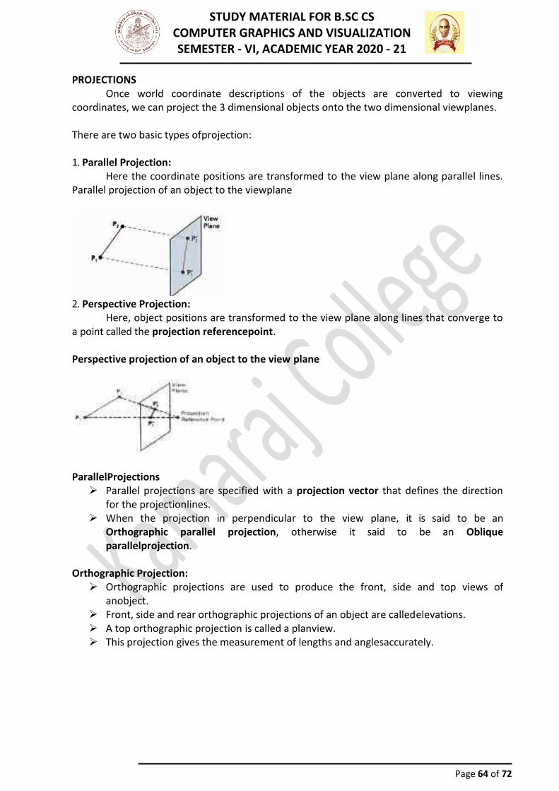
STUDY MATERIAL FOR B.SC CS COMPUTER GRAPHICS AND VISUALIZATION SEMESTER - VI, ACADEMIC YEAR 2020 - 21
Page 64 of 72
PROJECTIONS Once world coordinate descriptions of the objects are converted to viewing coordinates, we can project the 3 dimensional objects onto the two dimensional viewplanes. There are two basic types ofprojection: 1. Parallel Projection:
Here the coordinate positions are transformed to the view plane along parallel lines. Parallel projection of an object to the viewplane
2. Perspective Projection: Here, object positions are transformed to the view plane along lines that converge to a point called the projection referencepoint. Perspective projection of an object to the view plane
ParallelProjections
➢ Parallel projections are specified with a projection vector that defines the direction for the projectionlines.
➢ When the projection in perpendicular to the view plane, it is said to be an Orthographic parallel projection, otherwise it said to be an Oblique parallelprojection.
Orthographic Projection:
➢ Orthographic projections are used to produce the front, side and top views of anobject.
➢ Front, side and rear orthographic projections of an object are calledelevations. ➢ A top orthographic projection is called a planview. ➢ This projection gives the measurement of lengths and anglesaccurately.

STUDY MATERIAL FOR B.SC CS COMPUTER GRAPHICS AND VISUALIZATION SEMESTER - VI, ACADEMIC YEAR 2020 - 21
Page 65 of 72
Orthographic projections of an object, displaying plan and elevation views
The orthographic projection that displays more than one face of an object is called axonometric orthographic projections. ISOMETRIC PROJECTION
➢ The most commonly used axonometric projection is the isometricprojection. ➢ It can be generated by aligning the projection plane so that it intersects each
coordinate axis in which the object is defined as the same distance from theorigin.
Isometric projection for a cube ➢ Transformation equations for an orthographic parallel projection are straightforward. ➢ If the view plane is placed at position zvp along the zvaxis then any point (x,y,z) in
viewing coordinates is transformed to projection coordinatesasxp = x, yp = y where the original z coordinates value is kept for the depth information needed in
depth cueing and visible surface determinationprocedures. Oblique Projection
➢ An oblique projection in obtained by projecting points along parallel lines that are not perpendicular to the projectionplane.
➢ The below figure α and φ are twoangles.
➢ Point (x,y,z) is projected to position (xp,yp) on the viewplane. ➢ The oblique projection line form (x,y,z) to (xp,yp) makes an angle α with the line on the
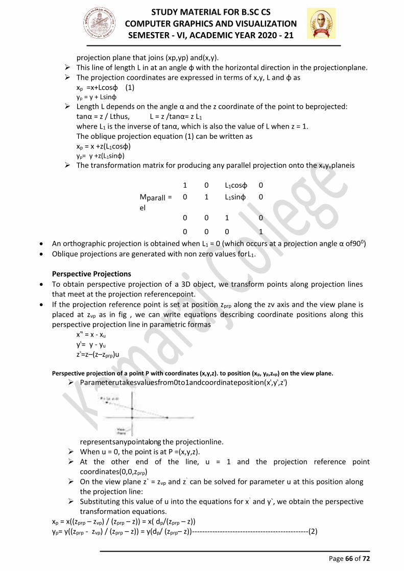
STUDY MATERIAL FOR B.SC CS COMPUTER GRAPHICS AND VISUALIZATION SEMESTER - VI, ACADEMIC YEAR 2020 - 21
Page 66 of 72
projection plane that joins (xp,yp) and(x,y). ➢ This line of length L in at an angle φ with the horizontal direction in the projectionplane. ➢ The projection coordinates are expressed in terms of x,y, L and φ as
xp =x+Lcosφ (1) yp = y + Lsinφ
➢ Length L depends on the angle α and the z coordinate of the point to beprojected: tanα = z / Lthus, L = z /tanα= z L1
where L1 is the inverse of tanα, which is also the value of L when z = 1. The oblique projection equation (1) can be written as xp = x +z(L1cosφ) yp= y +z(L1sinφ)
➢ The transformation matrix for producing any parallel projection onto the xvyvplaneis
1 0 L1cosφ 0
Mparallel
= 0 1 L1sinφ 0
0 0 1 0
0 0 0 1
• An orthographic projection is obtained when L1 = 0 (which occurs at a projection angle α of900)
• Oblique projections are generated with non zero values forL1.
Perspective Projections
• To obtain perspective projection of a 3D object, we transform points along projection lines that meet at the projection referencepoint.
• If the projection reference point is set at position zprp along the zv axis and the view plane is placed at zvp as in fig , we can write equations describing coordinate positions along this perspective projection line in parametric formas
x‟ = x - xu y‟= y - yu z‟=z–(z–zprp)u
Perspective projection of a point P with coordinates (x,y,z). to position (xp, yp,zvp) on the view plane.
➢ Parameterutakesvaluesfrom0to1andcoordinateposition(x‟,y‟,z‟)
representsanypointalong the projectionline. ➢ When u = 0, the point is at P =(x,y,z). ➢ At the other end of the line, u = 1 and the projection reference point
coordinates(0,0,zprp) ➢ On the view plane z` = zvp and z` can be solved for parameter u at this position along
the projection line: ➢ Substituting this value of u into the equations for x` and y`, we obtain the perspective
transformation equations. xp = x((zprp – zvp) / (zprp – z)) = x( dp/(zprp – z)) yp= y((zprp - zvp) / (zprp – z)) = y(dp/ (zprp– z)) ---------------------------------------------- (2)
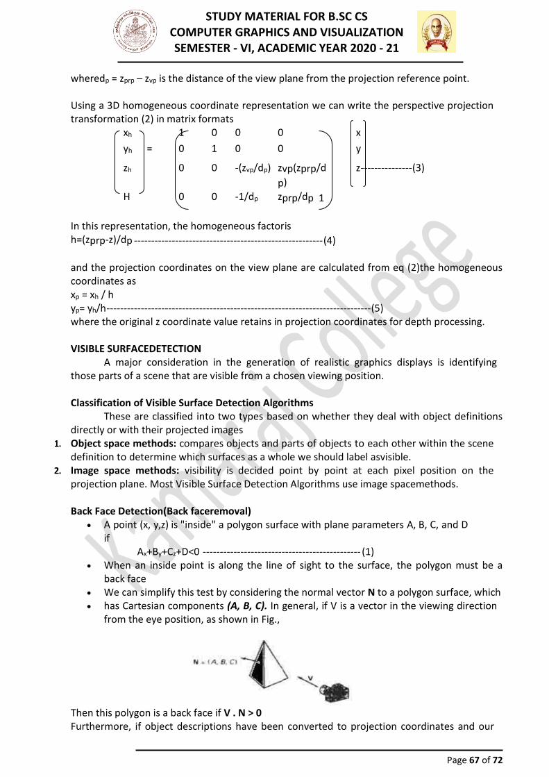
STUDY MATERIAL FOR B.SC CS COMPUTER GRAPHICS AND VISUALIZATION SEMESTER - VI, ACADEMIC YEAR 2020 - 21
Page 67 of 72
wheredp = zprp – zvp is the distance of the view plane from the projection reference point. Using a 3D homogeneous coordinate representation we can write the perspective projection transformation (2) in matrix formats
xh 1 0 0 0 x
yh = 0 1 0 0 y
zh 0 0 -(zvp/dp) zvp(zprp/d
p)
z --------------- (3)
H 0 0 -1/dp zprp/dp 1
In this representation, the homogeneous factoris h=(zprp-z)/dp ------------------------------------------------------- (4)
and the projection coordinates on the view plane are calculated from eq (2)the homogeneous coordinates as xp = xh / h yp= yh/h ----------------------------------------------------------------------------- (5) where the original z coordinate value retains in projection coordinates for depth processing. VISIBLE SURFACEDETECTION
A major consideration in the generation of realistic graphics displays is identifying those parts of a scene that are visible from a chosen viewing position. Classification of Visible Surface Detection Algorithms
These are classified into two types based on whether they deal with object definitions directly or with their projected images
1. Object space methods: compares objects and parts of objects to each other within the scene definition to determine which surfaces as a whole we should label asvisible.
2. Image space methods: visibility is decided point by point at each pixel position on the projection plane. Most Visible Surface Detection Algorithms use image spacemethods. Back Face Detection(Back faceremoval)
• A point (x, y,z) is "inside" a polygon surface with plane parameters A, B, C, and D if
Ax+By+Cz+D<0 ---------------------------------------------- (1) • When an inside point is along the line of sight to the surface, the polygon must be a
back face • We can simplify this test by considering the normal vector N to a polygon surface, which • has Cartesian components (A, B, C). In general, if V is a vector in the viewing direction
from the eye position, as shown in Fig.,
Then this polygon is a back face if V . N > 0 Furthermore, if object descriptions have been converted to projection coordinates and our
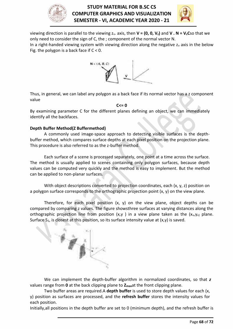
STUDY MATERIAL FOR B.SC CS COMPUTER GRAPHICS AND VISUALIZATION SEMESTER - VI, ACADEMIC YEAR 2020 - 21
Page 68 of 72
viewing direction is parallel to the viewing zv. axis, then V = (0, 0, Vz) and V . N = VzCso that we only need to consider the sign of C, the ; component of the normal vector N. In a right-handed viewing system with viewing direction along the negative zv axis in the below Fig. the polygon is a back face if C < 0.
Thus, in general, we can label any polygon as a back face if its normal vector has a z component value
C<= 0 By examining parameter C for the different planes defining an object, we can immediately identify all the backfaces. Depth Buffer Method(Z Buffermethod)
A commonly used image-space approach to detecting visible surfaces is the depth-buffer method, which compares surface depths at each pixel position on the projection plane. This procedure is also referred to as the z-buffer method.
Each surface of a scene is processed separately, one point at a time across the surface. The method is usually applied to scenes containing only polygon surfaces, because depth values can be computed very quickly and the method is easy to implement. But the method can be applied to non-planar surfaces.
With object descriptions converted to projection coordinates, each (x, y, z) position on a polygon surface corresponds to the orthographic projection point (x, y) on the view plane.
Therefore, for each pixel position (x, y) on the view plane, object depths can be compared by comparing z values. The figure showsthree surfaces at varying distances along the orthographic projection line from position (x,y ) in a view plane taken as the (xv,yv) plane. Surface S1, is closest at this position, so its surface intensity value at (x,y) is saved.
We can implement the depth-buffer algorithm in normalized coordinates, so that z
values range from 0 at the back clipping plane to Zmaxat the front clipping plane. Two buffer areas are required.A depth buffer is used to store depth values for each (x,
y) position as surfaces are processed, and the refresh buffer stores the intensity values for each position. Initially,all positions in the depth buffer are set to 0 (minimum depth), and the refresh buffer is
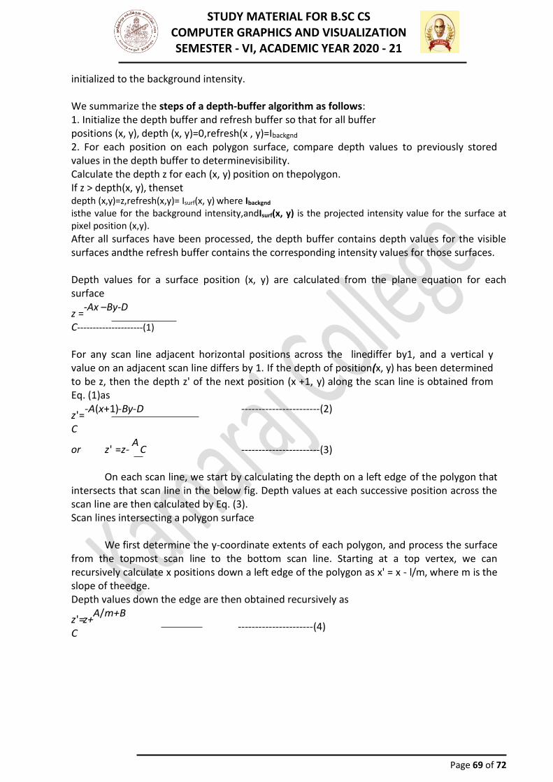
STUDY MATERIAL FOR B.SC CS COMPUTER GRAPHICS AND VISUALIZATION SEMESTER - VI, ACADEMIC YEAR 2020 - 21
Page 69 of 72
initialized to the background intensity. We summarize the steps of a depth-buffer algorithm as follows: 1. Initialize the depth buffer and refresh buffer so that for all buffer positions (x, y), depth (x, y)=0,refresh(x , y)=Ibackgnd 2. For each position on each polygon surface, compare depth values to previously stored values in the depth buffer to determinevisibility. Calculate the depth z for each (x, y) position on thepolygon. If z > depth(x, y), thenset depth (x,y)=z,refresh(x,y)= Isurf(x, y) where Ibackgnd
isthe value for the background intensity,andIsurf(x, y) is the projected intensity value for the surface at pixel position (x,y). After all surfaces have been processed, the depth buffer contains depth values for the visible surfaces andthe refresh buffer contains the corresponding intensity values for those surfaces. Depth values for a surface position (x, y) are calculated from the plane equation for each surface
z =-Ax –By-D
C---------------------(1) For any scan line adjacent horizontal positions across the linediffer by1, and a vertical y value on an adjacent scan line differs by 1. If the depth of position(x, y) has been determined to be z, then the depth z' of the next position (x +1, y) along the scan line is obtained from Eq. (1)as
z'=-A(x+1)-By-D
C
or z' =z- A
C
-----------------------(2) -----------------------(3)
On each scan line, we start by calculating the depth on a left edge of the polygon that
intersects that scan line in the below fig. Depth values at each successive position across the scan line are then calculated by Eq. (3). Scan lines intersecting a polygon surface
We first determine the y-coordinate extents of each polygon, and process the surface
from the topmost scan line to the bottom scan line. Starting at a top vertex, we can recursively calculate x positions down a left edge of the polygon as x' = x - l/m, where m is the slope of theedge. Depth values down the edge are then obtained recursively as
z'=z+A/m+B
C
----------------------(4)
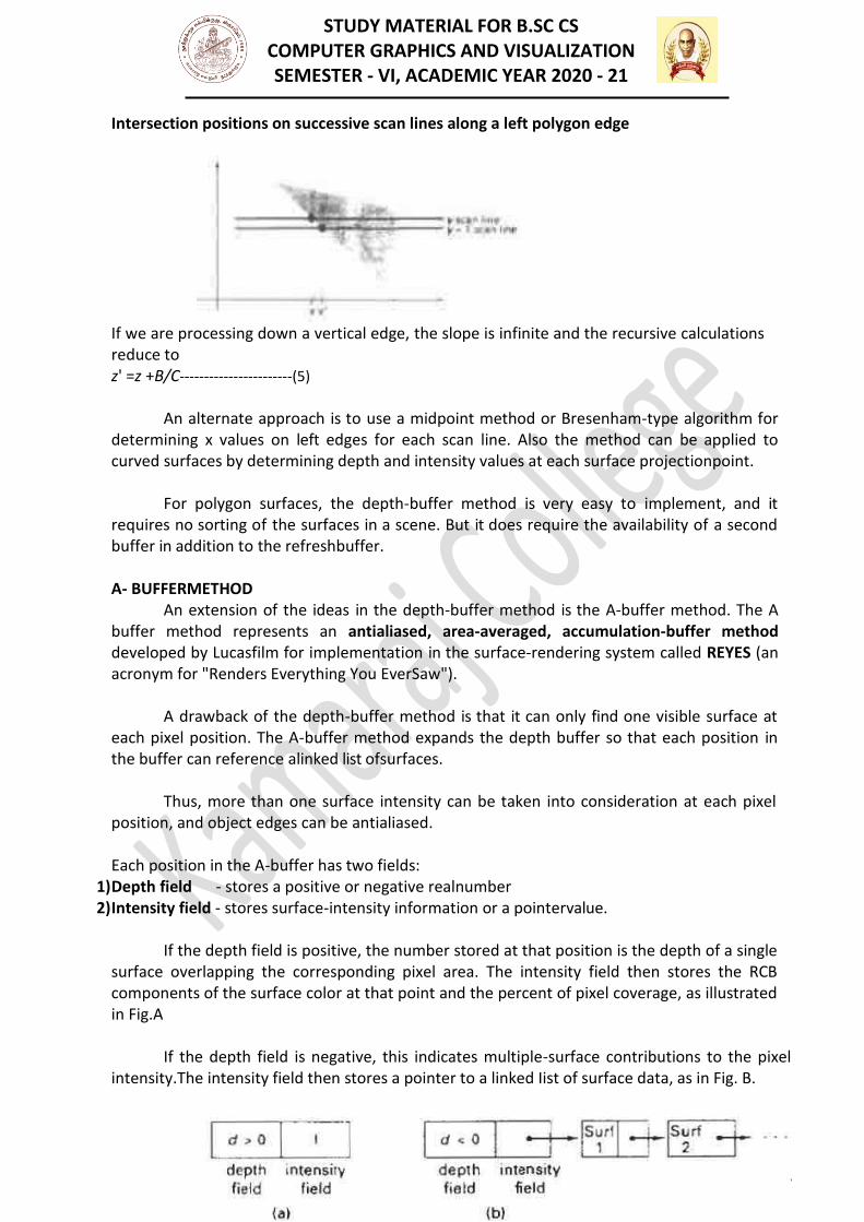
STUDY MATERIAL FOR B.SC CS COMPUTER GRAPHICS AND VISUALIZATION SEMESTER - VI, ACADEMIC YEAR 2020 - 21
Page 70 of 72
Intersection positions on successive scan lines along a left polygon edge
If we are processing down a vertical edge, the slope is infinite and the recursive calculations reduce to z' =z +B/C-----------------------(5)
An alternate approach is to use a midpoint method or Bresenham-type algorithm for
determining x values on left edges for each scan line. Also the method can be applied to curved surfaces by determining depth and intensity values at each surface projectionpoint.
For polygon surfaces, the depth-buffer method is very easy to implement, and it requires no sorting of the surfaces in a scene. But it does require the availability of a second buffer in addition to the refreshbuffer.
A- BUFFERMETHOD
An extension of the ideas in the depth-buffer method is the A-buffer method. The A buffer method represents an antialiased, area-averaged, accumulation-buffer method developed by Lucasfilm for implementation in the surface-rendering system called REYES (an acronym for "Renders Everything You EverSaw").
A drawback of the depth-buffer method is that it can only find one visible surface at each pixel position. The A-buffer method expands the depth buffer so that each position in the buffer can reference alinked list ofsurfaces.
Thus, more than one surface intensity can be taken into consideration at each pixel position, and object edges can be antialiased. Each position in the A-buffer has two fields:
1) Depth field - stores a positive or negative realnumber 2) Intensity field - stores surface-intensity information or a pointervalue.
If the depth field is positive, the number stored at that position is the depth of a single
surface overlapping the corresponding pixel area. The intensity field then stores the RCB components of the surface color at that point and the percent of pixel coverage, as illustrated in Fig.A
If the depth field is negative, this indicates multiple-surface contributions to the pixel intensity.The intensity field then stores a pointer to a linked Iist of surface data, as in Fig. B.
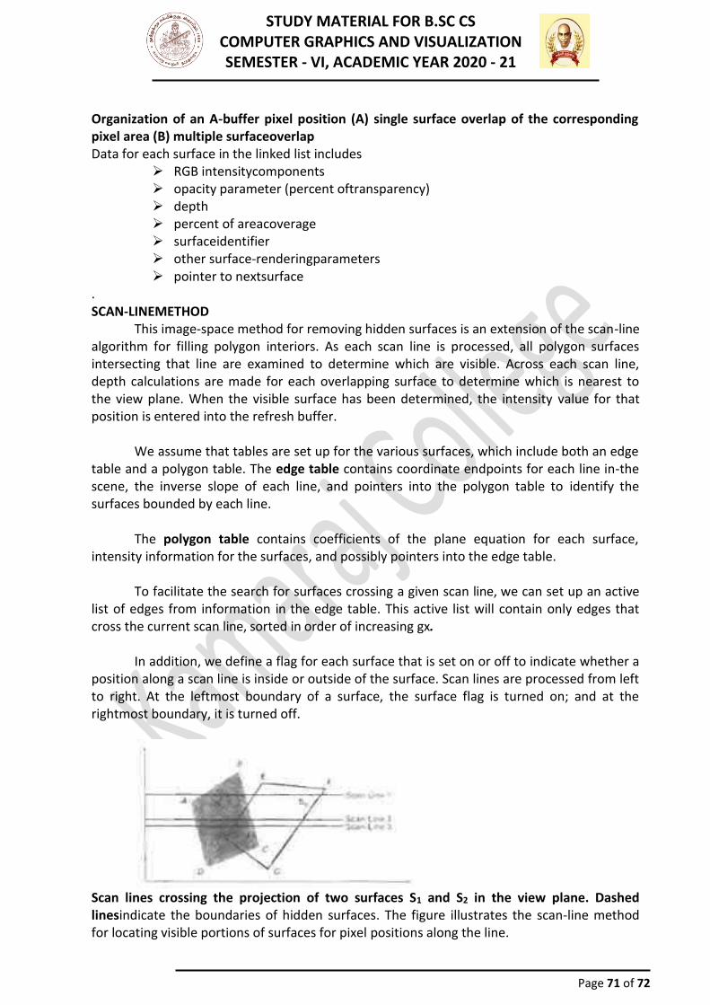
STUDY MATERIAL FOR B.SC CS COMPUTER GRAPHICS AND VISUALIZATION SEMESTER - VI, ACADEMIC YEAR 2020 - 21
Page 71 of 72
Organization of an A-buffer pixel position (A) single surface overlap of the corresponding pixel area (B) multiple surfaceoverlap Data for each surface in the linked list includes
➢ RGB intensitycomponents ➢ opacity parameter (percent oftransparency) ➢ depth ➢ percent of areacoverage ➢ surfaceidentifier ➢ other surface-renderingparameters ➢ pointer to nextsurface
. SCAN-LINEMETHOD
This image-space method for removing hidden surfaces is an extension of the scan-line algorithm for filling polygon interiors. As each scan line is processed, all polygon surfaces intersecting that line are examined to determine which are visible. Across each scan line, depth calculations are made for each overlapping surface to determine which is nearest to the view plane. When the visible surface has been determined, the intensity value for that position is entered into the refresh buffer.
We assume that tables are set up for the various surfaces, which include both an edge
table and a polygon table. The edge table contains coordinate endpoints for each line in-the scene, the inverse slope of each line, and pointers into the polygon table to identify the surfaces bounded by each line.
The polygon table contains coefficients of the plane equation for each surface,
intensity information for the surfaces, and possibly pointers into the edge table. To facilitate the search for surfaces crossing a given scan line, we can set up an active
list of edges from information in the edge table. This active list will contain only edges that cross the current scan line, sorted in order of increasing gx.
In addition, we define a flag for each surface that is set on or off to indicate whether a
position along a scan line is inside or outside of the surface. Scan lines are processed from left to right. At the leftmost boundary of a surface, the surface flag is turned on; and at the rightmost boundary, it is turned off.
Scan lines crossing the projection of two surfaces S1 and S2 in the view plane. Dashed linesindicate the boundaries of hidden surfaces. The figure illustrates the scan-line method for locating visible portions of surfaces for pixel positions along the line.
STUDY MATERIAL FOR B.SC CS COMPUTER GRAPHICS AND VISUALIZATION SEMESTER - VI, ACADEMIC YEAR 2020 - 21
Page 72 of 72
The active list for scan line 1 contains information from the edge table for edges AB, BC, EH, andFG.For positions along this scan line between edgesAB and BC, only the flag for surface S1 is on.
Therefore no depth calculations are necessary, and intensity information for surface S1, is entered from the polygon table into the refresh buffer.
Similarly, between edges EH and FG, only the flag for surface S2 is on. No other positions along scan line 1 intersect surfaces, so the intensity values in the other areas are set to the background intensity.
For scan lines 2 and 3 , the active edge list contains edges AD,EH, BC, and FG. Along scan line 2 from edge AD to edge EH, only the flag for surface S1, is on. But between edges EH and BC, the flags for both surfaces are on.
In this interval, depth calculations must be made using the plane coefficients for the two surfaces. For this example, the depth of surface S1is assumed to be less than that of S2, so intensities for surface S1, are loaded into the refresh buffer until boundary BC is encountered. Then the flag for surface S1 goes off, and intensities for surface S2 are stored until edge FG ispassed.
Any number of overlapping polygon surfaces can be processed with this scan-line method. Flags for the surfaces are set to indicate whether a position is inside or outside, and depth calculations are performed when surfaces overlap.