STUDY GUIDE FOR A BEGINNIN-G COURSE IN GROUND-WATER HYDROLOGY:

PART I -- COURSE PARTICIPANTS

L BOUNDARY OF FRESH ND-WATER SYSTEM

I BEDROCK

U.S. GEOLOGICAL SURVEY Open-File Report 90- 183

SECTION (4)--GROUND-WATER FLOW TO WELLS

Wells are our direct means of access or "window" to the subsurface environment. Uses of wells include pumping water for water supply, measuring pressures and heads, obtaining ground-water samples for chemical analysis, acting as an access hole for borehole geophysical logs, and direct sampling of earth materials for geologic description and laboratory analysis, primarily during the process of drilling the wells. Hydrogeologic investigations are based on these potential sources of well-related information.

Concept of Ground-Water Flow to Wells

Assignments

*Look up and write the definitions of the following terms relating to radial flow and wells in Fetter (1988), both in the glossary and in the index--drawdown, specific capacity of well, completely penetrating well, partially penetrating well, leaky confined aquifer, leaky artesian aquifer, semiconfined aquifer, and leaky confining bed or layer.

*Study Note (4-l) --Concept of ground-water flow to wells.

The general laws (Darcy's law and the principle of continuity) that govern ground-water flow to wells are the same as those that govern regional ground-water flow. The system concept is equally valid--we are still concerned with system geometry, both external and internal, boundary conditions, initial conditions, and spatial distribution of hydraulic parameters as outlined in table 1 of Note (3-2). However, the process of removing water from a vertical well imposes a particular geometry on the ground-water flow pattern in the vicinity of the well, which is called radial flow. Radial flow to a pumping well is a strongly converging flow whose geometry may be described by a particular family of differential equations that utilize cylindrical coordinates (r,z) instead of Cartesian coordinates (X,Y,Z) l A large number of analytical solutions to these differential equations with different boundary conditions describe the distribution of head near a pumping well.

Note (4-l). -TConcept of Ground-Water Flow to Wells

As has been noted previously, ground-water flow in real systems is three-dimensional. To obtain water from the ground-water system, wells are installed and pumped. Water pumped from the well lowers the water level in the well, thereby establishing a head gradient from the aquifer toward the well. As a result, water moves from the surrounding aquifer into the well. As pumping proceeds, a decline in head or drawdown propagates away from the well as water continues to move from areas of higher head to areas of lower head and is pumped out of the well.

; 130

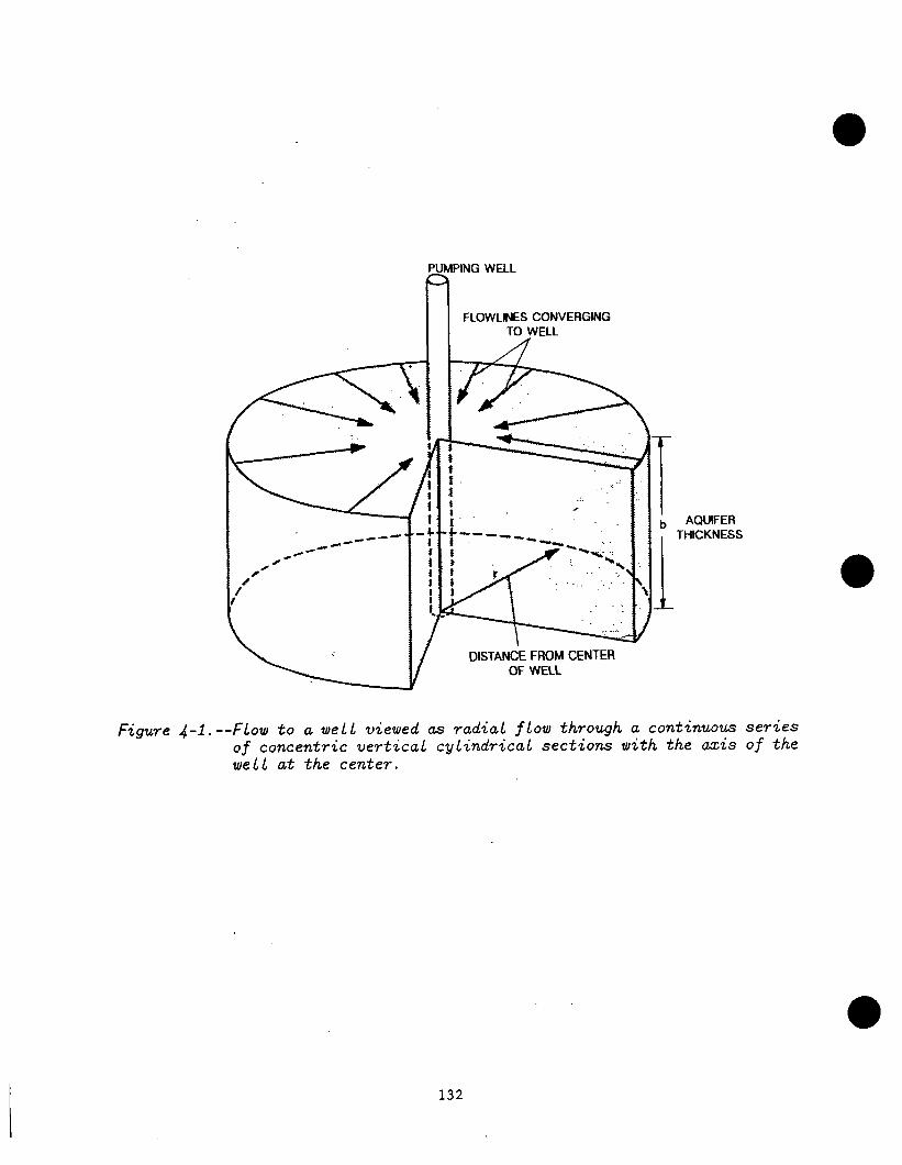
Ground-water flow to a pumping well can be viewed as occurring through a series of concentric vertical cylinders with the center of the well at the central vertical axis (fig. 4-l). If the aquifer properties (hydraulic conductivity (K) and storage coefficient (S)) are symmetric around the well, then the hydraulic head (or change in hydraulic head) and the flow of water (or change in flow) also will be symmetric. This symmetry enables us to simplify the analysis of a general three-dimensional flow system to a two- or one-dimensional system using cylindrical (or radial) coordinates.

Further consideration of figure 4-l indicates that flow to a well, or radial flow is a converging flow, because the areas of the concentric cylinders (A = Barb), which are perpendicular to the direction of ground-water flow, decrease continuously toward the well as the radial distance r from the center of the well decreases while the aquifer thickness b remains constant. If we apply Darcy's law conceptually to this flow system,

hl -b Q = KA s-_-m

1

where A = 2arb, and assume that Q and K are constant (that is, the flow system is in steady state and the aquifer is homogeneous), we can write

Q l-9 -h, - = _____ = constant A K 1

We have seen that the area perpendicular to ground-water flow decreases toward hl -hz

the well. Thus, for the above relation to be true, the head gradient ----- 1

must increase continuously toward the well. This qualitative inference from Darcy's law is a general and characteristic feature of flow to wells. Equations that define this increase in gradient toward the pumping well are developed in subsequent notes and exercises.

Because pumping wells may be located in diverse hydrogeologic environments, quantitative analysis of the associated radial-flow systems requires the use of simplifying assumptions. Our conceptualization of the system, based on the distribution of the transmitting and storage properties of the aquifer and the boundary conditions of the radial section under study, determines how the radial flow system is simplified and formulated for analysis. For example, transmitting and storage properties vary depending on whether the aquifer in question is one homogeneous aquifer, a heterogeneous layered aquifer, or a complex aquifer system. Boundary conditions, such as a partially penetrating well that causes significant vertical movement, or an impermeable top and bottom of the aquifer as opposed to a "leaky" top and bottom, also affect the complexity of the system to be analyzed.

All radial flow systems can be conceptualized in a variety of ways, each of which leads to a different simplification that is incorporated into a mathematical description of the system. As shown in figure 4-2(A), a well pumping in a multi-aquifer system could be studied in the context of the entire aquifer system, and the head and flow throughout the system could be

131

PUMPING WELL

r

I FLOWLINES CONVERGING I TO WELL

f

f t I’

_:_

s

DISTANCE FROM CENTER OF WELL

AQUIFER THICKNESS

Figure 4-l. --Flow to a well viewed as radial flow through a continuous series of concentric vertical cylindrical sections with the axis of the well at the center.

.32

Upper boundary ,(impermeable or free surface)

EXPLANATION

. . RADIAL CROSS SECTION OF AQUIFER TO BE SIMULATED

a WELL SCREEN

A. ANALYSIS OF ENTIRE AQUIFER SYSTEM

LEAKY TOPBOUNDARY

\ LEAKY BOTTOM BOUNDARY from center)

B. ANALYSIS OF THE PUMPED AQUIFER

Figure d-2. --Two conceptualizations of the same ground-water system.

133

simulated huantitatively by means of a numerical model. Or, the problem could be conceptualized by assuming that the pumping would not affect significantly the aquifer system above and below the extensive confining units. In this situation the flow system could be analyzed as a single aquifer that receives leakage from the overlying and underlying aquifers through the confining beds (fig. 4-2(B)). In case A, the entire multi-aquifer system is defined as the system under study, while in case B, only the aquifer being pumped is analyzed.

The notes and problems that follow describe the use of mathematical solutions for different radial flow conceptualizations. Keep in mind the internal characteristics and boundary conditions of the various radial-flow models and solutions that are discussed; these features determine the degree to which the mathematical representation of the flow system corresponds to the real, physical flow system.

Analysis of Flow to a Well --Introduction to Basic Analytical Solutions

Assignments

*Study Note (4-2)--Analytical solutions to the differential equations governing ground-water flow.

*Study Fetter (1988), p. 143, 199-201; Freeze and Cherry (1979), p. 188-189, 314-319; or Todd (1980), p. 112-113, 115-119, 123-124.

*Study Note (4-3) --Derivation of the Thiem equation for confined radial flow.

*Work Exercise (4-1)--Derivation of the Dupuit-Thiem equation for unconfined radial flow.

*Study Fetter (1988), p. 161-169.

*Study Note (4-4) --Additional analytical equations for well-hydraulic problems.

This subsection is primarily a study section that provides an introduction to some of the simplest and most widely applied radial-flow equations. We focus on three such equations-- (1) the Thiem equation for steady-state confined flow, (2) the Dupuit-Thiem equation for steady-state unconfined flow, and (3) the Theis equation for unsteady confined flow. These and all other radial-flow equations relate to specific, highly idealized ground-water flow systems. We cannot overemphasize the importance of learning the key features of the individual flow systems to which each equation applies. These key features relate in large part to the boundary conditions that are assumed in the derivation of a given equation.

134

Note (4-2) .--Analytical Solutions to the Differential Equation-s $‘overning Ground-Water Flow

This note reviews and extends some of the ideas discussed in a previous note on the information required to describe a ground-water system (Note 3-2).

Quantitative analysis of a ground-water flow problem involves the definition of an approprlate boundary-value problem. Definition of a boundary-value problem requires the specification of the governing differential equation and the initial and boundary conditions applicable to the specific problem under study. The governing differential equation is a mathematical model that describes ground-water flow in the flow domain. The information needed to define a boundary-value problem involving ground-water flow is shown in table 4-l (reproduced from table 3-1, Note 3-2) in the context of a simple system diagram.

Solution of a boundary-value problem involves solving the governing differential equation (generally a partial-differential equation in ground-water flow problems) for the initial and boundary conditions that apply to the problem. Today, complex boundary-value problems generally are solved by numerical methods with the assistance of a digital computer. However, many useful analytical solutions to boundary-value problems representing simple systems are available.

An analytical solution to a ground-water problem is an exact mathematical solution to a specific boundary-value problem that is relevant to ground-water studies. We may think of an analytical solution as a "formula" amenable to calculation that relates the dependent variable in the differential equation (generally head (h) or drawdown (s) in ground-water problems) to the independent variable(s) in the differential equation (coordinates of position (x,y,z) and time (t)). Thus, an analytical solution may be represented in a general way as

h = f(x,y,z,t).

An analytical solution is an exact solution to the governing differential equation, and provides a formula that permits calculation of the dependent variable in continuous space and time. However, analytical solutions usually are available only for highly idealized conceptualizations of ground-water systems. Thus, the solution to the idealized mathematical representation (governing differential equation and boundary conditions) is exact, but the mathematical representation rarely corresponds closely to hydrogeologic conditions in the real system.

Some of the typical simplifying assumptions used in the mathematical model to develop analytical solutions are (a) flow medium (earth material) is isotropic and homogeneous, (b) the aquifer is confined, (c) the aquifer is unbounded laterally (infinite area1 extent), and so on. Furthermore, the geometry of the flow system generally is simple--for example, the flow system is bounded by a rectangular or circular prism, the aquifer is horizontal and of constant thickness, the well completely penetrates the aquifer, and so on. Finally, boundary conditions usually are simple (constant head, no-flow, and constant flux are common boundary conditions).

135

Table 4-l. z- Information necessary for quantitative definition of a ground-water flow system in context of a general system concept l

Input ---------------->> System -me---- ------->>Output

Input or stress applied Factors that define the Output or response of to ground-water system ground-water system ground-water system

(1) Stress to be analyzed: (1)

- expressed as volumes of water added or withdrawn

- defined as function (2) of space and time

(3)

(4)

External and internal (1) Heads, drawdowns, geometry of system or pressures' (geologic framework)

-defined as - defined in space function of

space and time Boundary conditions

-defined with respect to heads and flows as a function of location and time on boundary surface

Initial conditions

-defined in terms of.heads and flows as a function of space

Distribution of hydraulic conducting and storage parameters

- defined in space

1 Flows or changes in flow within parts of the ground-water system or across its boundaries sometimes may also be regarded as a dependent variable. However, the dependent variable in the differential equations governing ground-water flow generally is expressed in terms of either head, drawdown, or pressure. Simulated flows across any reference surface can be calculated when the governing equations are solved for one of these variables, and flows in real systems can be measured directly or estimated from field observations.

136

Even with all their simplifications, analytical solutions can provide invaluable hydrologic insight into idealized but nevertheless representative and relevant ground-water systems. Furthermore, they often can be used effectively in the quantitative analysis of ground-water problems (for example, analysis of aquifer tests). In general, no analytical solution corresponds exactly to a given field situation. Thus, a proper application of analytical solutions to field problems requires that the hydrologist have a detailed understanding of the physical system represented by the analytical solution and the assumptions (the most important assumptions often involve boundary conditions) that underlie the analytical solution.

Note (4-3). --Derivation of the Thiem Equation for Confined Radial Flow

Darcy's law describes the flow of water through a saturated porous medium and can be written as follows (Fetter, 1988, p. 123, equation 5-19):

dh Q = - KA __

dr

where A is the cross-sectional area through which the water flows, r is distance along the ground-water flow path (in this case, radial distance), and the other terms are as previously defined. Steady flow to a well (fig. 4-3) in a confined aquifer bounded on top and bottom by impermeable units is radially convergent flow through a cylindrical area around the well. As shown in figure 4-3, the area (A) through which flow occurs is

A = Zarb,

where b is the thickness of the completely confined aquifer. Substituting this expression for A into Darcy's law gives:

dh Q = -2lrKbr -- .

dr

For steady flow, Q, the constant quantity of water pumped from the well, is also the flow rate through any cylindrical shell around the well.

This equation can be solved by separating variables and integrating both sides of the equation. Separation of variables gives:

1 2rKb _ dr = _ __-- dh. r Q

Integrating from r2 to rl, where the heads are h, and h,, respectively,

dr I

IT2 -- = rl r ,/

, ,'

,’ I,, /

137

SUlgA~L c - -

- - Q = CONSTANT WELL DISCHARGE

0 /

I SCREENEI INTERVAL OF WELL

I

/- / -

/’ / 1’ /

h

IMPERMEABLE CONFINING UNIT

r

AQUIFER

+- 4

c

6

Q b = AQUIFER THICKNESS

4

Note: h is head in aquifer above datum at radial distance r; Q is constant well discharge which equals constant radial flow in aquifer to well; r is radial distance from axis of well; Z is elevation head.

FigzLre d-9. --Steady flow to a completely penetrating well in a confined aquifer.

138

gives

or

27rKb In r2 - In rl = - ---- (h, - h,),

Q

r2 2aKb Ln -- = - ---- (h, - h,).

r1 Q

Rearranging terms gives

4 T2 Kb = -------_--- In -- .

2T(hg - hl 1 rl

Because Kb equals transmissivity (T) and the pumping rate is defined as a positive number, the resulting equation is

Q r2 T= ----------- In -- ,

2a(h, - hl 1 rl

which is the Thiem equation as given by Fetter (1988, p. 200, equation 6-56).

Exercise (4-l) --D erivation of the Dupuit-Thiem Equation for Unconfined Radial Flow

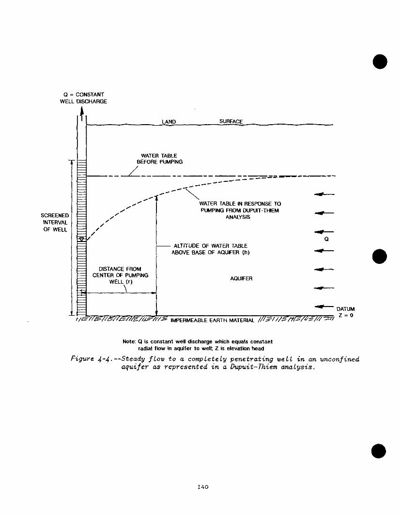
The Dupuit-Thiem equation (Fetter, 1988, p. 200, eqation 6-57) for unconfined radial flow is analogous hydrologically to the Thiem equation for confined radial flow (Note 4-3). Review Note 4-3 and derive the Dupuit-Thiem equation using a similar sequence of steps. The key difference between this derivation and the derivation of the Thiem equation lies in expressing the cylindrical area of flow around a pumping well in an unconfined aquifer as A = 2nrh (fig. 4-4), as opposed to A = 2%rb for confined flow, where h is the saturated thickness of the unconfined aquifer at a distance r from the pumping well. Expressed in another way, the datum or reference elevation for h is at the bottom of the unconfined aquifer, which is assumed to be an impermeable \ boundary (fig. 4-4).

139

Q = CONSTANT WELL DISCHARGE

SCREENED INTERVAL OF WELL

LAND SURFACE

WATER TABLE BEFORE PUMPING

/ -- --_-__-__-__-__ _4--- -- ----,-----

DISTANCE FROM CENTER OF PUMPING

‘*‘-’ ’ (0 WCLL AQUIFER

\ c

-WATER TABLE IN RESPONSE TO PUMPING FROM DUPUIT-THIEM

ANALYSIS

- ALTITUDE OF WATER TABLE ABOVE BASE OF AQUIFER (h)

t ~//E/&lz=iz/5 IMPERMEABLE EARTH MATERIAL ///-=/i/3 /%=/--=I# =i’7

DATUM Z=O

Note: Q is constant well discharge which equals constant radial flow in aquifer to well; Z is elevation head

Figure 4-4.--Steady flow to a completely penetrating well in an unconfined aquifer as represented in a Dupuit-Thiem analysis.

140

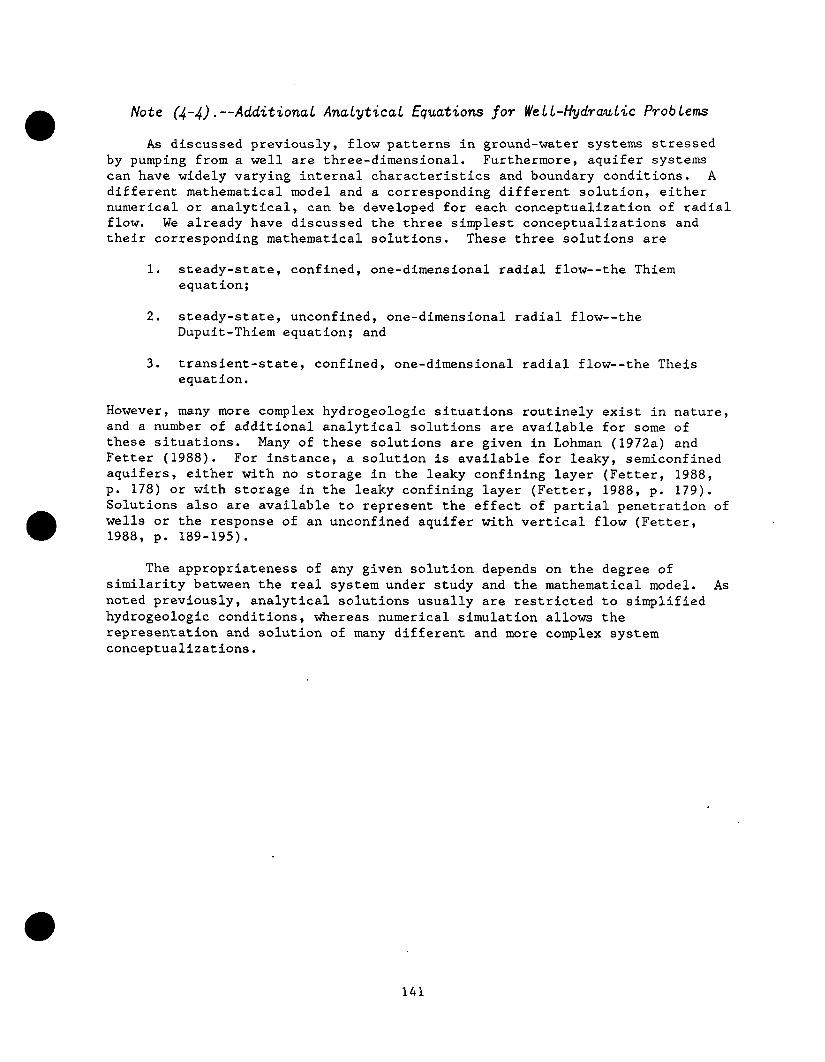
Note (4-4). --Additional Analytical Equations for We 11-Hydraulic Problems

As discussed previously, flow patterns in ground-water systems stressed by pumping from a well are three-dimensional. Furthermore, aquifer systems can have widely varying internal characteristics and boundary conditions. A different mathematical model and a corresponding different solution, either numerical or analytical, can be developed for each conceptualization of radial flow. We already have discussed the three simplest conceptualizations and their corresponding mathematical solutions. These three solutions are

1. steady-state, confined, one-dimensional radial flow--the Thiem equation;

2. steady-state, unconfined, one-dimensional radial flow--the Dupuit-Thiem equation; and

3. transient-state, confined, one-dimensional radial flow--the Theis equation.

However, many more complex hydrogeologic situations routinely exist in nature, and a number of additional analytical solutions are available for some of these situations. Many of these solutions are given in Lohman (1972a) and Fetter (1988). For instance, a solution is available for leaky, semiconfined aquifers, either with no storage in the leaky confining layer (Fetter, 1988, p. 178) or with storage in the leaky confining layer (Fetter, 1988, p. 179). Solutions also are available to represent the effect of partial penetration of wells or the response of an unconfined aquifer with vertical flow (Fetter, 1988, p. 189-195).

The appropriateness of any given solution depends on the degree of similarity between the real system under study and the mathematical model. As noted previously, analytical solutions usually are restricted to simplified hydrogeologic conditions , whereas numerical simulation allows the representation and solution of many different and more complex system conceptualizations.

141

Analysis of Flow to a Well--Applying Analytical Solutions to Specific Problems

Assignments

*Study Fetter (1988), p. 170-199; Freeze and Cherry (1979), p. 343-349; or Todd (1980), p. 125-134.

*Work Exercise (4-2)--Comparison of drawdown near a pumping well in confined and unconfined aquifers using the Thiem and Dupuit-Thiem equations.

*Work (a) the example problem in Fetter (1988), p. 165, and (b) using the same data as in (a), determine the radial distance at which the drawdown would be 0.30 meters after 1 day of pumping.

*Work Exercise (4-3)--Analysis of a hypothetical aquifer test using the Theis solution.

In this subsection we apply the analytical solutions introduced in the previous section to some typical problems. Additional problems, some that require other analytical solutions, are available in Fetter (1988) at the end of chapter 6.

Exercise (4-2) --Comparison of Drawdown Near a Pumping We1 1 in Confined and Unconfined Aquifers Using the Thiem and Dupuit-Thiem Equations

The purpose of this exercise is to (1) become more closely acquainted with the Thiem and Dupuit-Thiem equations by using them in numerical calculations and (2) contrast the response to stress (pumping) of a linear (confined) ground-water system and a nonlinear (unconfined) ground-water system. The concept of system linearity or nonlinearity refers to the relationship between system stresses, such as changes in pumping or recharge, and system response, as measured by changes in heads or drawdowns. For example, in a linear system, doubling the pumping rate of a given well in steady-state conditions, doubles the drawdown at every point in the neighborhood of that well. The response of a ground-water system to stress is inherently nonlinear if the geometry of the system changes in response to the stress. Common examples of changes in system geometry in response to stress are (1) changes in the elevation of the water table, (2) changes in the position of a freshwater-saltwater interface, and (3) changes in the length of a stream in hydraulic connection with the ground-water system.

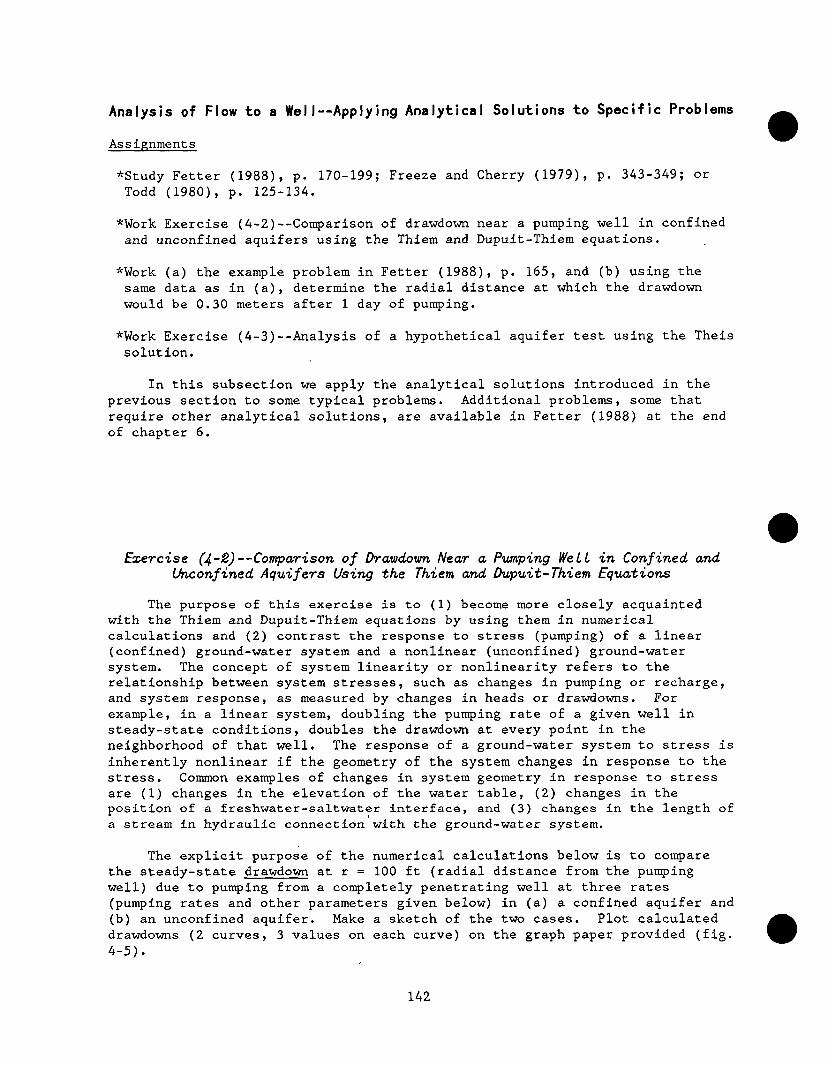
The explicit purpose of the numerical calculations below is to compare the steady-state drawdown at r = 100 ft (radial distance from the pumping well) due to pumping from a completely penetrating well at three rates (pumping rates and other parameters given below) in (a) a confined aquifer and (b) an unconfined aquifer. Make a sketch of the two cases. Plot calculated drawdowns (2 curves, 3 values on each curve) on the graph paper provided (fig. 4-5).

142

Pumping rates: Q1 = 25,920 fta/d, Q* = 51,840 fta/d, e = 103,680 ft=/d.

Confined Case (Thiem equation)

K= 50 ftlday

b (aquifer thickness) = 75 ft

r, ("radius of influence")' = 10,000 ft (assume the head is constant at this distance)

r (radial distance from pumping well at which calculations of head and drawdown will be made) = 100 ft

hinitial (head in aquifer before pumping begins) = he = 200 ft

Unconfined Case (Dupuit-Thiem equation)

K = 50 ftlday

re = 10,000 ft

r = 100 ft

h initial (saturated thickness of unconfined aquifer before pumping begins) = 75 ft

First, write the appropriate formula and solve algebraically for the unknown head before inserting numerical values. Then calculate drawdown.

(1) Suppose that the initial head in the confined aquifer is 500 ft instead of 200 ft. Would this change in initial head have any effect on the result of your calculation of drawdown?

(2) Write a careful description of the two curves plotted in figure 4-5.

1 The phrase "radius of influence" of a pumping well is loosely defined, but implies a distance from the pumping well at which the head is constant in all radial directions or the drawdown in response to that particular stress either is so small that it cannot be measured or becomes impossible to distinguish from "background noise" in the aquifer. In calculations with the Thiem and Dupult-Thiem equations, the "radius of influence" is the assumed or approximated distance from the pumping well at which head remains constant at the prepumping level.

143

. : : . : :

-...: . . . . . . . . . . . ..-. _...,.._.; . . ..i . . . . . . . . . . is..

: : : : : : . . . . . . . . . .

- . ..w............- - . . . . . . . . . . . . . - . . . . . _ s.....

: : : : . . : :

: : : : . .

: :

. . : : : : .

: : : : . .

- . ..-...e......... -...a..._ . . . . . . . . . . . . . . . . . . . .

: : : .

: : : :

: i :

.._r....,.... ;...- . . . . . . ..-. _._...-..; . . . . . . . .

I-“‘~” .:: . . . . . . . . . . . . . . ...“” . . . . . . . . . . . . . -.. : : : : . . .

- $...i . . . . . . . . . i . . . . . . . . . J . . . . j...; . . . . . . . . . j.- L I : : : : 1 : : : :

: : : *

t.

: : ._ . . . . . . . . . . . . . . _....m

: . : ; i

f :

. . . . . . . . . . :..e..._ . ..-.

: : : : . . .

ii ir./....; . . . . . . . . . ;...!“..; ._.. [..!?..

v .l__..; . .._ L . . . . . .._. J . . . . i....i....: . . . . :,..

/ i ; . .

h i i i i i

0 v) 0 T-

.._

. . .

. . .

. . .

,.-; . . . . . . . . . . _._.; -...

: : : :

. .

. . . . _ . . . . . . . . “.” ..-.

: : : .

. . . ..-.... . . . . . ..-....--,

: : :

. . . .

. . . . . . ..I.... -..-a...

: : : :

: * . : : : .

: : : :

: . . . ._.._. .e. . . ..-.-. . . . .

: : : :

: : ..__I . ..-....-, -.-.A:---

.

: : : . .__.........-_...-.._

. : : :

. : : . . _ . ., . . . . , . . . _. . . . ., . . .

. : : :

. . .

. . . : : : :

. . . .:. . .-; _. . .:. . . _ ‘.. .

: : : : . . .._........ L.......

. : : .

. . _ ;: . . . . , . . . .,- . f . -. . . . : : :

: : :

. : : :

, : . . ..-: _...: . .._ ,.-‘<...

: : : . -..:. . . .;. . .-:... .I..-

: : : . .

._ _.....: . . . . L...:...

: 9 ; .

._ . .._... :...A:- . . . . ..-.

, : : : . . . .

: . : . . . ..I . . . . . e...: . . . . . ..-.

: ; : . . . .._-....: . . . . y...:... : . * * . .

: : :

. . . . . . . . )-m-s: .,...; . . . .

: : : . . . .

.___........ -...e . . . .

: : : : . . . . . . . . . . . . . . . . . .._. :.-..

: . : .

: : :

. . . . . . . . . . . . . . . . . .

..-____.._...-_.......-.-.-...-.-, . . . I : : : : . . . . . . . . . ,..._.....,._ _ : : : : . , . . - . ,. . . . , . . : : : : .

. . ..__.... . . . . . . . .._....-. -...a..

: : : : : :

..; ._.. ;....__ _ . . . . . _ .,....~.._..,. _ : : : :

: : : : : : .... .... .... .... .... .... : : : : : :

. . . . .__.; . . . . . . . . . . . . . . . . ..-. . . . . :...

: : : . . :

: : . .

._*...._. ___... _._.. . . . . . . . . ..- s.....

: : : : ;

. ..i . .._ -: . . ..i ._..i .-.......; . . . . :...

. .

: : : : : :

-I . . . . . . ..__..... . . . . . . . . . . . . . . ;..

: : : : . . . . . .

.._ _._... _..-._s...-..s..- __.. _-

: : : : : .

. : : : ..: . . . . ..-...-.....-.. i-~ . . . . . . . ..-.

. . .

: : : : : : : : : : : :

._~_...~__....___C...,.......__~.....___......._..._.......~__....

: : : : : : : : : : : :

: : :

: : : :

: ; :

: :

: : ; :

:

: :

. . . . . : . . . : .

. : : : : I :

. . : : : : . : ; ; ,...........__.....-_.. _ . . . . . . . . - . . . . .._........._-... _ -....-...- _. : . : : : : : : : : : : : : ,.._I . . . . . . .-..,....,.... : : : : : : : . . . . . ..-..........--..-....-....... :.- ..,.... _.. : : : : : : : : . : : : .... ( .... ....

.... .... .... : : : : . . . :.-.-.: . . . . . . . . . . . . . . J. .-! . . ;... . . . . ,....I.....: .._. i....i __.. ,.. ,.. ._

. . . . . . . . . . . . . . . . . . . ..-........i....-...1.......................-...~.. . : : : : : : : : : : :

: : : : . .

. : * : . : : . . , .

. . .

. : : : . :

. 1

: : : . . . .

.___.. ~“:--~““..-“.

: :

. . . . . . . . . y..‘........ _.._ _..... _ . .._.m......

: I : I i

: : : : . : : ; . . .

____: . . . . . :--..;-...: . . . . . . . . . . . . . ‘s....‘.... ,.... _ ..-.: . . . ..-.... . . . . . . _. : :

i ; I i , , , I : : : . . : . I I i i I 1

, :: z

. : :

. .

: : : : . : : :

. . . . . . . . . .

_...____...._.__. _-._ . ..-..._.f_ - . . . .._.... _ . . . . _ . . . ..-... _...A......

. : : :

. .

: : : : : : : :

. *

: : . : : :

: : : : : : : .

. . . . . . : : : *

. . . . . . .

. .

. .

. .

. .

. .

. .

. . .

. .

. .

. .

.

. .

. .

. .

. .

. . ,.. . . . . .

.- ,

. . i

. . i . . -; s

1333 NI ‘113M YyOtIJ 1333 001 = J IV NMODMVtKl

144

Exercise (4-3)--Analysis of a Hypothetical Aquifer Test Using the Theis So Lution

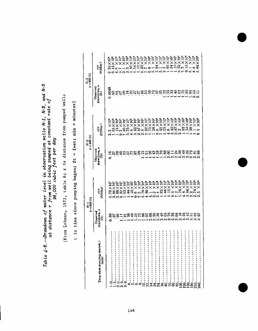
The purpose of this exercise is to use the Theis solution to determine the aquifer properties T and S by curve-matching. Drawdowns at three wells spaced 200, 400, and 800 ft from a well pumping at a rate of 96,000 fta/d are listed in table 4-2 (from Lohman, 1972).

(1) Plot the aquifer-test data in table 4-2 on log-log paper in two ways--(a) drawdown (s) against time (t) using data from a single well (any one of the three observation wells) on figure 4-7, and (b)'drawdown (s) against t/r2 using data from all three observation wells on figure 4-8. In general, if data from more than one observation well are available, alternative (b) is preferable. Calculate t/r2 by either taking the reciprocal of r*/t in table 4-2 or performing the calculation directly from the data given.

(2) Overlay the Theis type curve (fig. 4-6) onto each plot of test data and determine a match point. Use the values obtained from the match point and equations 6-3 and 6-4 in Fetter (1988, p. 164) to determine the transmissivity (T) and storage coefficient (S) of the aquifer. To facilitate the calculations, equation 6-3 can be rearranged as

Q T= --- W(u)

4lr.s

0 and equation 6-4 as

t S = 4Tu l -- .

r*

Concept of Superposition and Its Application to Well-Hydraulic Problems

Assignments

*Study Fetter (1988), p. 201-204; Freeze and Cherry (1979), p. 327-332; or Todd (1980), p. 139-149.

*Study Note (4-5) --Application of superposition to well-hydraulic problems.

*Work Exercise (4-4) --Superposition of drawdowns caused by a pumping well on the pre-existing head distribution in an area1 flow system.

Superposition is a concept that has many applications to ground-water hydrology as well as to other physical systems that are described by linear differential equations. We use superposition when we analyze (most) aquifer tests, perhaps without realizing this fact, and in the theory of images and image wells. Superposition also has applications to the numerical simulation of ground-water systems, a topic that is not discussed in this course.

145

146

4 ‘- l- 0

oJ)M

147

..:--:...:..i...~-...: . . . . . . t . .._...... .:-.I..>-;..i...: . . . . j . . . . . . . . _ . . . . . . . . . . ;.i..:..: . . . . . . . i . . . . . . . . . . . i..-- . . . . . ._.__._.._ ..~.~.~..~...:‘.“l~ . . .._ :_ . . . . . . _ ._.. ~.~.~..]..~..<..-.~ . . . . . . . . . . _._ . . . . !-:.t.-..-.:...:..-‘.......

/...: .*..:....-.. < . . . .._._....._..... ~.‘..~..~ . . . . . . . “..:‘.- -.-: . . . . . . . . . . . . ~.~.~..:‘..:“‘:~“.~~ . . . . . . ..--.. _., ;__i__:_ .!.. ;...; . .._. ____..; . ..---.-....<. < ..:.. :...:-..: . . . . > . . . . . . :...- . . . . . . . . i-b.) .‘.. ‘.-.~..-‘.-..--?..--.-...

. . . . . . . . *. . . . :...: .m..t.-.“.. :..- ___._...._.___,. :.y: ._._..; . . ..I ..__..; . . . . . . . . . ...! _ ..f.‘“..i . . ..-- -.:- . . . . . . . . . _ . . . . ,::: . : . .:::: ,._I ._,_. i-.;...>...; ___... > . ..____..... :.r..; . . . . ..i . . . . . . . . . . . . . . . . . . . _ . . . . . . . . ).:.:.-I . . . . . . . . ..-........ :- . . . . . _..- ::::: : : . . . . .

. : : . : : “::: : : . .

:.:..:-r..:...;...: . .._.. . ,.................... L.-i..-: . . . . ;-m-.-z . . . . . . . . . . . . . . . . . . . . ..~...i....~....-.....-..-. ::::: : : i .‘.: . , : : : : ‘.::’ : . . : “::: : * : ,..: : : : “:: . . . :::

:..:..:..;..:...: . . . . . _._......... _ .._... ;.:.;..:..: ..-.-...: . . . . . . . _- . . . . . . . . . . :.;.:..: ..-...; . . . . :. . . . . . . . . . . ..-A. ::::: : : :::: : : : ‘.::: . : . :‘::: : . , : : : 9 .:::. :

: : : *

::: i : ..: : : . . .:::. : .

.::.: : : : : * :.: .

: ‘. *:: . . *

. . . . . ::::: : :

. ,..... . . . . . . . . : . :..>.:..i..;...>.--; .._._. > .._..._. -...:-;..:..:...I..;...~~..-~.~..~-~ . . . . . . . ;.~.;..:...:.-.i.-.~: . . . . . . i . . . ..-.. _ ~.~.:..~~~~..‘~ . . ..I . . . . . . . . . . _ -..- m-,.:-b:- y-s. L......~....‘......~.~...~~~....~.~~~..’-..~...~‘..~....‘~’.~’~.‘~’ ,__,__ 2 .._.! __....__! . . . . . . :..._ _.._.... ~.~‘~..~““.‘,....~ . . . . . i ,_.........I .!...‘.“..: . . . . __._:_ _.............. . :..i.-:...:..:.-.i-..-: ..___. f . . . . . . .._... :..:..:..i..~...:....! ....._ :..-..-....--i-!-l.-i...:.--!-.--:.-----!.---..--.

. . . . . . ..*.*. ;.:..;..:..i ___...._: .____.: . ..___._.... ~‘~.~~.~..~..~ ..-.: . . . . . :.-- . . . . . . . . . :.:.: .-,. -“-.: . . . . ;.- . . . . :-- . ..-. -.

: : ::: : * : ,.++.. _._i___ -..\ ._.__.......i .-,_ -...* ..:...: ‘...:.‘.“‘.. _ :. .

. . ..-......-!-...:-.~...i.--.;-....i.........

: . : : . *..: . . : : “::: : : . . :..;..I..;..:...: . . . . :.. __..I . . . . . . . . . . ..i.............: .._. :...-..:..-- . . . . . . . . . . . . . :-.I .--‘-..i.--...-....i-....-.-- “.:: ’ : .::: : : : ..: .:: :::,: : :

. . ::::: : :::

:: :

. . . i .;. r..:m.;.s.ym..; . . . . . . . __.___...... >.:..>.;..t..-:- . ..i.....l......-.......i.;..~..:...i--..~-....i.. . . .._.f

._ . . . .’ . . _. !..- .____! _......______....__ ~.~.~..~.“..< . . . . “ . . . . f ._.......... !.~.!“-.‘“‘~“‘.~ .-.. -.: . . . . . -... . . ~...;.~~.~.~~...~~..~..~.~~........,”-.~..~.~..~...~....~’~~”.~.....~.“.“~~~.~..:“.:“.~““~’.”’~...~.“” >.y.: ..!.. ;--q . . ..I _____.; .._._.___.. -<.;.<-.:...f..; . . . . . . . . . . . . . . ..--...... ;.:.;--:...:-..: . . . . . .-..-. > .--......

. . . . . . . . . . . . . . :.-.: . . ..!..“... <...- _..._._____.... I’:.: .!.. :...; -...: . . . ..-. . . . . . . . . . ..-. .:.:.. :..i.. .:....: .--..: . . . . . . . -. .: :.. : : :..:.-:..:..i...~.-.; ___... > . . . .._...... :.:.;..:...;.... -.......-.... ..:: : *. . : :::: . ,:: .::: : : :

._ . . . . . . . . . . I.:..; . . . . . . . . . . / . . . . .._..__. . . . . . . . . :.‘. : . : ::.:. -.... ~ --...... _: ..__: ._____ i ..____ _ ._... :.;..:..:..;-.-.-..i-....-.-------.-..:.,-:--.-..:---,---.r---.-,..---.---

: . :::: * .::: : : : . : :::: : : i :.: : : . .

. : : : :

,:_ . . . .._ . , _. : . . .:. . . . . . . - _ ::: :

..: . . . . . . . . . . . . . :.;.;..:..: . . . . . . . . . . . . . . . . ..::: : :

..__........ ;.: _.,._: ..-...; . . . . . . . . . . . ;. . . . . . . . ::::: : : : “::: . : ::::: : .

:::: i .:: : : : ..::. : . . :

:‘: : : : : ::: : : : . : .

.’ : : . :::

.:::: : ::*,. .

; .:: : . . . . . . : ‘. : : I . :::

. . . . . ::. .: ..:.. :-.i..;.em :_._ -; ____. _:_.._____ .-.-.: -;..:-.;--‘.-; . . . . I . . . . . . . ._... _ . . . . . . ;.:..;-.:...:...:..--.: . . . . . . . . . ..-..-. . . . . . . _.,.. f . . . .._..I . . . . . . . . . . . . . . . . . . . y.:..y.f . . . . ..I . . . . . . . . . . . . . . . . . . . . . . . . ~...‘..:‘..~..~ . . . . b-.-..:..- . . . . . .

.:..:..:..;..:...: . . . . f--.m.e ._._____ __ ___d _ ,.__. ‘““.‘< _._. :“T.‘i-..--.- . . . . *

v) l- In l-

r

1333 NI ‘6) NMOCIMVHCI

148

::::: : . . . . .::: : : :I..: :

.:: . .:... .

.:-.:--:--i-.i---~-- _I______ :----- ______ .... ..-’ ..; ... .; ... ..; .......... JL......~.~~~.~ .. .._ . .

. . . ..I-.-.-........-.

.! -...: . . .._ -)-..--.---

. .

. . . ..~.........__..._

. . .

+.- .._..._ j.........

. .

. . . . . . . . ..i.........

. . .,.-.~--..-.;..-.---. : : : * : : .

1333 NI ‘6) NMOClMVtJQ

c

149

Note (4-5). --Application of Superposition to Well-Hydraulic Problems

To simplify the analysis of ground-water flow to wells we have assumed until now that heads and flows around the well axis are radially symmetrical. However, heads and flows are not always symmetrical around the axis of a well. If a regional gradient exists, the head upgradient from the well is higher than the head downgradient from the well. However, the change in head (the drawdown) and the change in flow due to pumping still are symmetrical about the well.

Using the theory of superposition (Reilly and others, 1987), we can analyze most well-hydraulic problems in terms of drawdowns and changes in flow. The theory of superposition states that, for linear systems, the solution to a problem involving multiple inputs (or stresses) is equal to the sum of the solutions for each individual input or stress. A more formal definition of superposition is that if Y, and Y, are two solutions to a linear differential equation with linear boundary conditions, then C,Y, + C,Y, is also a solution, where C, and C, are constants.

Superposition allows us to avoid analyzing the actual heads and to analyze only the drawdown. The Theis solution given by Fetter (1988, p. 164, equation 6-3) is stated in terms of drawdown (he-h) as

ha-h = ;z; W(u).

This equation is a solution to the governing differential equation which is given in terms of head by Fetter (1988, p. 162, equation 6-1) as

a2h 1 ah S ah --- + - -- = - --, at? r ar T at

The principle of superposition allows this equation to be written in terms of the changes in head (or drawdowns) that occur in the system as

a2 (&j-h) 1 wh,-h) s a($+) -e--w - -,- + - ------- = - -------9

h-2 r ar T at or

62 s 1 as s as --- + - -- = - -- 63 r ar T at

150

0

0

where s is the drawdown. This formulation greatly simplifies the mathematical solution because the initial conditions1 are a constant zero drawdown everywhere at the start of pumping, and the drawdown is radially symmetrical.

A more complete explanation of superposition and a set of problems is available in Reilly, Franke, and Bennett (1987).

Exercise (4-4)--Superposition.of Drawdowns Caused by a t%.unping .WeLL on the Pre-Existing Head Distribution in an Area1 Flow System

In Note 4-3, we derived the Thiem equation in terms of absolute head. In this form of the Thiem equation, the head at some radial distance from a pumping well must be the same in all directions. Through the use of superposition (Note 4-5), the Thiem equation can be applied to more general field situations in which drawdowns are radially symmetric even if absolute heads are not.

The Thiem equation from Note 4-3 is

T= --i-Q---- In (rz/rl). 2rr(h, -h, >

We can represent the head at points 1 and 2 by

h, = b-sl, and

where h,, is the original head before onset of pumping, and s is the drawdown. Substituting these equations into the Thiem equation gives

T= ----Q---- In (r2/rl). 21Tt.59 -s2 1

Assuming that the drawdown s2 is negligible at some distance, r,, from the pumping well and rearranging gives:

Sl = -Q_ In (re/rl). 2aT

This form of the Thiem equation gives the drawdown, sl, at any radial distance, rl, from the pumping well.

1 In analyses of ground-water systems, "initial conditions" means specifying the head distribution throughout the system at some particular time. These specified heads can be considered to be reference heads; calculated changes in head through time are relative to these given heads, and the time represented by these reference heads is the reference time. For further discussion of initial conditions see Franke, Reilly, and Bennett (1987).

151

A uniform head (potential) distribution in a hypothetical confined aquifer of uniform transmissivity, T, is shpwn in figure 4-9. Determine the future potential distribution under steady-state conditions in response to a pumping well centered in the figure at the square. Assume that there is no drawdown at a distance, r,, of 5,000 ft, for a well pumping at 9,090 ft3/d. The transmissivity of the aquifer is 1,000 ftg/d.

We will calculate drawdowns and the predicted new heads at locations marked with circles and labeled with letters in figure 4-9. Perform the calculations and contour the new head distribution using the following sequence of steps:

Calculate drawdowns--Use table 4-3 to calculate the drawdowns at various distances from the pumping well. Note that the locations of all 30 reference points are defined by only six radial distances, r, from the pumping well.

Calculate absolute heads--Use table 4-4 to calculate the new head at each reference point. Determine the initial prepumping head from the contour lines given in figure 4-9. Determine the distance of the observation point from the pumping well, and transfer the appropriate drawdown from table 4-3. Finally, subtract the drawdown from the initial head for each reference point.

Contour new potentiometric surface-- Plot the new heads on figure 4-10 and contour, using a 1-ft contour interval.

As an aid in contouring the new potentiometric surface, consider the original potentiometric surface in figure 4-9 and draw a dashed line on figure 4-9 that is perpendicular to the head contour lines and passes through the location of the pumping well. Because these initial head contour lines are parallel straight lines, the new potentiometric surface resulting from steady pumping of the well will be symmetrical about the dashed line. Draw a dashed line at the same position on figure 4-10 and observe that the potentiometric surface being contoured is symmetric about this line. This new potentiometric surface shows the effect of the discharging well.

(1) Based on available head data, estimate the position of the ground-water divide on the dashed line in figure 4-10. Starting at this point on the divide, sketch two upgradient streamlines, one on each side of the well, making the assumption that these streamlines are perpendicular to the existing head contour lines. Sketch two or three additional streamlines between the first two streamlines and the well. What is the significance of the first two streamlines? What is the area upgradient from those first two streamlines called?

(2) The drawdown at reference point T is 2.84 ft. Is the direction of flow at T toward or away from the discharging well? Explain why the water at this point is flowing in a direction away from the discharging well despite significant drawdowns at wells X, T, S, and Y.

152

. . . . . : . . , . ‘,. . . . . , . . : . : . . ; . . : . ._. . , . . : . . , . . , . . : . . , . . ;

153

Table 4-3. --Format for calculation of drawdowns at specified distances from the pumping we 11

fre is distance from pumping well at which drawdown is negligible; r1 is distance from pumping well at which drawdown equals sl; fi,~ is natural logarithm; Q is pumping rate of well; T is transmissivity of aquifer]

-Q Preliminary calculation: --- = constant =

2nT

250

500

I I

707 I I 1

1000

1118

I 1414 I

154

Table 4-4. --Format for calculation of absolute heads at specified reference points

WELL INITIAL DISTANCE DRAWDOWN HEAD = INITIAL IDENTIFICATION PREPUMPING FROM WELL DUE TO HEAD-DRAWDOWN,

LETTER HEAD (FEET) (r), IN FEET IN FEET

A

I3

C

D

E

F

G

H

I

J

K

L \

M 1

N

155

.,. ._...

156

.

Aquifer Tests

Assipnments

+Study Fetter (1988), p. 204-209; Freeze and Cherry (1979), p. 335-343, 349-350; or Todd (1980), p. 45-46, 70-78.

*Study Note (4-6)--Aquifer tests.

One of the main activities of ground-water hydrologists is to estimate physically reasonable values of aquifer parameters for different parts of the ground-water system under study. The most powerful- and direct field method for obtaining aquifer parameters is a carefully designed, executed, and analyzed aquifer test. Unfortunately, aquifer tests are labor- and time-intensive. Often, the most important decision in connection with an aquifer test is whether or not to perform one--in other words, whether the value of the test data equals the cost of obtaining those data. This generally is a difficult question to answer.

Note (4-6). --Aquifer Tests

An aquifer test is a controlled field experiment that is designed to determine the hydraulic properties of an aquifer and (or) associated confining beds. The most common type of aquifer test involves pumping a well at a constant rate to stress the aquifer, monitoring the drawdown response of the aquifer, and analyzing these data. The-analysis usually assumes radial symmetry and uses either an analytical solution to the conceptually appropriate mathematical model or a mathematical-numerical model solved by computer.

Stallman (1971, p. l-3) discusses the philosophy and general procedure of aquifer tests succinctly. HQ outlines the general procedure in terms of three phases --test design, field observations, and data analysis. It is critically important that the test be designed with an initial conceptualization of the system and a proposed method of analysis. The conceptualization of the system may change as analysis proceeds; then different methods of analysis may be required.

As noted previously, many analytical solutions to well-hydraulic problems exist. For example, Reed (1980) gives analytical solutions and type curves for 11,different cases of flow to wells in confined aquifers. However, analytical solutions tend to describe the response of simplified homogeneous systems. Therefore, numerical simulation sometimes is required to estimate the hydraulic properties of the aquifer being tested. Simulation usually is used in a trial-and-error manner, changing aquifer and confining bed coefficients in a systematic and physically reasonable way based on previous knowledge or simplified analyses (for example, analyses using analytical solutions), until an acceptable match between the observed response of the aquifer and the simulated response is achieved.

157