STUDY FOR THE COMPUTATIONAL RESOLUTION OF …

1

STUDY FOR THE COMPUTATIONAL RESOLUTION OF CONSERVATION EQUATIONS OF MASS, MOMENTUM

AND ENERGY

REPORT

Student: David Comerón Castillo Bachelor’s Degree in Aerospace Vehicles Engineering Director: Asensio Oliva Llena Co-Director: Carlos-David Perez Segarra Delivery date: 10th June 2019.

3

ACKNOWLEDGMENTS

I would like to thank everyone who has helped me develop this project, in one way or another. First, thank all the CTTC (Centre Tecnòlogic de Transferència de Calor) crew, especially professor Carlos David for the support he has given, guiding me through the realization of the project. Also, thank my family for always being there when I needed them, encouraging me to work on this thesis and giving me their best advice. Lastly, thank my friends for also supporting me and give a helping hand in whatever thing they could.

4

ABSTRACT

The main purpose of this project is the creation of a CFD program able to solve the Navier-Stokes equations. Before the realisation of this program, other programs solving different problems will be created, like a 2D heat conduction program, a potential flow program and a convection-diffusion program. After those are done and validated, the Navier-Stokes solving program will be done. This program must also be validated, so the results obtained are reliable.

6

INDEX

CHAPTER 1. INTRODUCTION ....................................................................................... 11

1.1 AIM ........................................................................................................................................... 11

1.2. REQUIREMENTS ..................................................................................................................... 11

1.3. SCOPE ..................................................................................................................................... 11

1.4 JUSTIFICATION AND STATE OF THE ART ........................................................................... 12

CHAPTER 2. NUMERICAL METHODOLOGY ............................................................... 13

2.1 INTRODUCTION ....................................................................................................................... 13

2.2 DISCRETIZATION METHODS.................................................................................................. 15

2.2.1 FINITE ELEMENT METHOD (FEM) .......................................................................................... 15

2.2.2 FINITE DIFFERENCE METHOD ............................................................................................... 16

2.2.3 FINITE VOLUME METHOD ...................................................................................................... 16

2.3 NUMERICAL SCHEMES .......................................................................................................... 18

2.3.1 UPWIND DIFFERENCE SCHEME ............................................................................................ 19

2.3.2 CENTRAL DIFFERENCE SCHEME ......................................................................................... 19

2.3.3 HYBRID DIFFERENCE SCHEME ............................................................................................. 19

2.3.4 EXPONENTIAL DIFFERENCE SCHEME ................................................................................. 20

2.3.5 QUICK SCHEME ...................................................................................................................... 20

2.4 TEMPORAL SCHEMES ........................................................................................................... 21

2.4.1 EXPLICIT .................................................................................................................................. 21

2.4.2 IMPLICIT................................................................................................................................... 21

2.4.3 CRANK-NICHOLSON ............................................................................................................... 21

2.5 SOLVERS ................................................................................................................................. 21

2.5.1 GAUSS-SEIDEL ....................................................................................................................... 22

7

2.5.2 TDMA ....................................................................................................................................... 23

2.5.3 LINE BY LINE ........................................................................................................................... 24

CHAPTER 3. TEST CASES AND RESULTS ANALYSIS .............................................. 25

3.1. INTRODUCTION ....................................................................................................................... 25

3.2 HEAT CONDUCTION ............................................................................................................... 25

3.2.1 HEAT CONDUCTION EQUATIONS ........................................................................................ 25

3.2.2 SPATIAL AND TEMPORAL DISCRETIZATION ......................................................................... 26

3.2.3 PROBLEM DEFINITION: 2D TRANSISTENT PROBLEM ........................................................... 27

3.2.4 RESOLUTION METHOD ............................................................................................................. 28

3.2.5 RESULTS AND CONCLUSIONS ................................................................................................. 33

3.2.6 PARALELIZED CASE: 1D TRANSISTENT PROBLEM .............................................................. 37

3.3 POTENTIAL FLOW ........................................................................................................................ 39

3.3.1 POTENTIAL FLOW EQUATIONS ............................................................................................... 39

3.3.2 EQUATIONS DISCRETIZATION ................................................................................................. 40

3.3.3 PROBLEM DEFINITION .............................................................................................................. 41



3.4 CONVECTION-DIFFUSION ............................................................................................................ 50

3.4.1 CONVECTION-DIFFUSION EQUATIONS ................................................................................... 50

3.4.2 TEMPORAL AND SPATIAL DISCRETIZATION .......................................................................... 51




3.5 NAVIER-STOKES........................................................................................................................... 63

8

3.5.1 THE NAVIER-STOKES EQUATIONS .......................................................................................... 63

3.5.2 FRACTIONAL STEP METHOD ................................................................................................... 64


3.5.4 PROBLEM RESOLUTION ........................................................................................................... 70


CHAPTER 4. BUDGET AND ENVIROMENTAL IMPACT .............................................. 80

4.1 BUDGET ........................................................................................................................................ 80

4.2 ENVIROMENTAL IMPACT ............................................................................................................. 84

CHAPTER 5. CONCLUSIONS AND FUTURE WORK ................................................... 85

5.1 CONCLUSIONS ............................................................................................................................. 85

5.2 FUTURE WORK ............................................................................................................................. 85

CHAPTER 6. REFERENCES .......................................................................................... 87

9

LIST OF FIGURES

Figure 1. Example of an ANSYS CFD simulation of a racing car. .......................................................... 12

Figure 2. General scheme for numerical resolution of a physical problem. ............................................ 13

Figure 3. Finite element method linear approximation of a function ....................................................... 15 Figure 4. Scheme of a node centred, Cartesian, structured and collocated mesh. ................................ 18

Figure 5. Tri-diagonal matrix general nomenclature .............................................................................. 23

Figure 6. 2D heat condutction problem geometrical scheme ................................................................. 27

Figure 7. Mesh used for the discretization of the domain of all problems. .............................................. 29

Figure 8. Resolution scheme for the 2D heat conduction case .............................................................. 32

Figure 9. Temperature map of the 2D heat conduction case with 4 materials with different physical properties. 80x80 nodes. ....................................................................................................................... 33 Figure 10 Temperature map of the 2D heat conduction case, with 1 material. 80x80 nodes ................. 34

Figure 11. Temperature map of the 1D heat conduction case with analytical solution. 80x80 nodes. .... 36

Figure 12. Comparison between the temperatures of the numerical simulation and the analytical solution of the 1D heat conduction case ............................................................................................................. 37

Figure 13. Scheme of the velocities nomenclature of a control volume for the potential flow resolution. 40

Figure 14. Scheme of the potential flow problem to be solved. .............................................................. 42

Figure 15. Resolution scheme of the potential flow problem. ................................................................. 46 Figure 16. Velocity module field for the flow around a cylinder, using 100x100 nodes. .......................... 47

Figure 17. Stream function map of the flow around a cylinder case, using 100x100 nodes. .................. 48

Figure 18. Stream function map of the analytical solution of the potential flow around a cylinder. ......... 49

Figure 19. Smith-Hutton problem definition scheme. ............................................................................. 53

Figure 20. Resolution scheme of the Smith-Hutton problem. ................................................................. 57

Figure 21. Comparison between reference and simulated results for the Smith-Hutton problem, 𝜌Г = 10 ............................................................................................................................................................. 59

Figure 22. Comparison between reference and simulated results for the Smith-Hutton problem, 𝜌Г =10𝑒3 .................................................................................................................................................... 59

Figure 23. Comparison between reference and simulated results for the Smith-Hutton problem, 𝜌Г =10𝑒6 .................................................................................................................................................... 60

Figure 24. Map of Ф for the Smith-Hutton problem, with 𝜌Г = 10 ....................................................... 61

Figure 25. Map of Ф for the Smith-Hutton problem, with 𝜌Г = 10𝑒3................................................... 61

Figure 26. Map of Ф for the Smith-Hutton problem, with 𝜌Г = 10𝑒6................................................... 62 Figure 27. Staggered mesh structure and location of the velocity components...................................... 66

Figure 28. Scheme of the driven cavity case, to be solved with the fractional step method. .................. 69

Figure 29. Scheme of the staggered mesh cells and corresponding boundary nodes velocities. ........... 71

Figure 30. Resolution scheme of the Navier-Stokes equations, using the fractional step method. ......... 74

10

LIST OF TABLES Table 1. Physical properties of the different materials for the 2D heat conduction case ......................... 28

Table 2. Boundary conditions values for the flow around a cylinder potential flow problem ................... 42

Table 3. Values of different variable parameters to convert the generic convection-diffusion equation into the Navier-Stokes equations ................................................................................................................. 50 Table 4. Boundary conditions for the Smith-Hutton problem. ................................................................. 54

Table 5. Values of 𝐴(𝑃) for the different numerical schemes as a function of the Peclet number ......... 56

Table 6. Different 𝜌Г values solved for the Smith-Hutton problem. ....................................................... 58

Table 7. Comparison of the reference and simulated results for the Smith-Hutton problem, for different 𝜌Г values ................................................................................................................................................... 58

Table 8. Comparison between the reference and the simulated results for the X component of the velocity at the middle vertical line of the driven cavity case ................................................................................ 79

Table 9. Comparison between the reference and the simulated results for the Y component of the velocity at the middle horizontal line of the driven cavity case ............................................................................ 78

Table 10. Hours spent on each task during the project .......................................................................... 82 Table 11. Initial Gantt table planning ..................................................................................................... 81

Table 12. Gantt table planning that was actually followed, done after the realisation of the project........ 82

Table 13. Planned future activities to be done for the project. ............................................................... 86

11

CHAPTER 1. INTRODUCTION 1.1 AIM

The main goal of this project is the numerical resolution of the Navier-Stokes equations in order to create a CFD (Computational Fluid Dynamics) program in C++, able to solve a particular case of an aeronautical or industrial problem. In addition, before taking on the practical cases, do a study of the theoretical background and solve some reference problems, which its solution is known in order to validate and verify the codes created.

1.2. REQUIREMENTS

The requirements for this project are listed below:

- The program developed must be written in C++ or C coding language. - The program must be able to solve numerically the Navier-Stokes, and be able to run

in a laptop. - Computational cost must be as low as possible. - The code must be self-made.

1.3. SCOPE

The tasks and activities that have to be done in order to complete this project are the following:

- A little research and study on the computational resolution of the Navier-Stokes equations.

- Develop a program able to solve conduction problems in 1D and 2D in a transient

regime. - Develop a program able to solve potential flow problems. - Develop a code in order to solve generic convection-diffusion equations. - Develop a CFD program able to solve the Navier-Stokes equations. - Modify the CFD program to make it resolve and optimize an industrial or aeronautical

problem.

12

- Study the viability of the resolution of the problem studied.

1.4 JUSTIFICATION AND STATE OF THE ART

Many of the engineering problems nowadays imply solving some kind of differential equations. Those equations, especially the ones that include partial derivatives, are hardly ever solved analytically, mostly because those problems do not have a known analytical solution. In the case of fluid dynamics, the equations governing the fluid motion are the Navier-Stokes equations, a set of partial derivative differential equations without a known analytical solution. Then, in order to solve this problems, a valid approach is using numerical methods and, in the case of fluid dynamics, using computational fluid dynamics. Even though the results of a problem obtained numerically are not exact, they are a good enough approximation to get valid results applicable to real world problems. Up until the late 20th century, since the computational power was insufficient, the numerical approach was just a theoretical way to solve those seemingly impossible to solve problems. However, with the recent increase in the late 20th century and early 21st of the computational power, these numerical methods were dusted off and given a primary role in the fluid dynamics. Nowadays, computational engineering is a key component of the fluid dynamics and heat transfer subjects, and is present in a lot of technical aspects. CFD is progressively taking ground off laboratory experiments, those last being more expensive. The main aim of this project is having a first contact with CFD programs, try to understand how they work by doing one yourself, and to interpret the results obtained.

Figure 1. Example of an ANSYS CFD simulation of a racing car.

13

CHAPTER 2. NUMERICAL METHODOLOGY

2.1 INTRODUCTION

As it has been stated in the introduction, a way to solve the Navier-Stokes equations is using numerical simulations. In this section, some of the numerical methods to approach the problems presented during the numerical resolution of the Navier-Stokes equations will be explained.

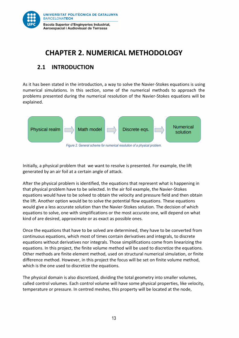
Figure 2. General scheme for numerical resolution of a physical problem.

Initially, a physical problem that we want to resolve is presented. For example, the lift generated by an air foil at a certain angle of attack. After the physical problem is identified, the equations that represent what is happening in that physical problem have to be selected. In the air foil example, the Navier-Stokes equations would have to be solved to obtain the velocity and pressure field and then obtain the lift. Another option would be to solve the potential flow equations. These equations would give a less accurate solution than the Navier-Stokes solution. The decision of which equations to solve, one with simplifications or the most accurate one, will depend on what kind of are desired, approximate or as exact as possible ones. Once the equations that have to be solved are determined, they have to be converted from continuous equations, which most of times contain derivatives and integrals, to discrete equations without derivatives nor integrals. Those simplifications come from linearizing the equations. In this project, the finite volume method will be used to discretize the equations. Other methods are finite element method, used on structural numerical simulation, or finite difference method. However, in this project the focus will be set on finite volume method, which is the one used to discretize the equations. The physical domain is also discretized, dividing the total geometry into smaller volumes, called control volumes. Each control volume will have some physical properties, like velocity, temperature or pressure. In centred meshes, this property will be located at the node,

14

situated at the centre of the cell. In staggered meshes, the property of the value is located at the node face, instead of in the middle of the cell. The way the geometry is discretized, will generate different types of meshes, structured on unstructured, quadrilateral or triangular, centred or staggered… In this project the meshes used will be structured, quadrilateral and centred, except for the case of the Navier-Stokes resolution, in which the method used is defined for a staggered, centred quadrilateral mesh. Moreover, the time is also discretized. Depending on the temporal discretization scheme, the temporal convergence and the result will be affected. Some of those temporal discretization schemes are implicit, explicit, crank Nicholson… and will be explained with detail later on another section. Even though the value of the property of interest will be located at the node, sometimes will be useful to know the value of that property at the face of a cell instead of at the node. To calculate the value, different numerical schemes are used, like CDS, EPS, QUICK… Those numerical schemes will be explained in detail in following sections. In this project, the most used will be CDS and EPS. Most of the times, the discretized equations end up being a system of algebraic equations, with 1 equation for each control volume. A solver is a method to solve this large system of equations. They can be direct or iterative, and will be studied with more detailed in future sections. Once the discretized equations are solved, a numerical solution will be obtained. This solution will be a set of numbers which will represent the value of the properties we’re looking for at each control volume. This will be a discrete solution, not a continuous one. Also, depending on different factors, like the mathematical equation used, the mesh size, or the equation discretization method used, the result can vary significantly. However, all the results obtained will be approximate solutions, since some errors are made. Modelling errors are made when going from the physical realm to the mathematical model. Discretization errors are committed from the mathematical model to the discretized equations, and solver residual round-off errors are made when solving the discretized equations. However, the result is often good enough to have a real world application or some relevant conclusions.

15

2.2 DISCRETIZATION METHODS

Discretization is the process of converting a continuous equation into a discrete equation. It is usually a first step towards the numerical resolution of that initial equation. However, when an equation is discretized, some errors are made. The goal is to make this error as small as possible. In this section, three discretization methods will be explained: Finite Element Method (FEM), Finite Difference Method (FDM) and Finite Volume Method (FVM). Nevertheless, since the method used in this project to program is the FVM, the focus will be set on that method, while the other two will be briefly explained.

2.2.1 FINITE ELEMENT METHOD (FEM)

The finite element method is a numerical method widely used to solve structural, heat transfer or fluid flow problems. This method converts a differential equation into a system of algebraic equations. The large system is sub-divided into smaller ones which are called finite elements. The function ruling the whole domain is then spitted among the finite elements, creating a lot of much simpler functions. The equations that model those finite elements are then assembled into a system of algebraic equations that can be solved. This method has several advantages:

- Accurate representation of complex geometries

- Inclusion of different material properties

- Capability to capture small local effects

- Relatively simple representation of the global solution

Figure 3. Finite element method linear approximation of a function

16

2.2.2 FINITE DIFFERENCE METHOD

The finite difference method is a numerical method able to solve differential equations by approximating them with difference equations, where derivatives are approximated. That method converts a differential equation into a system of algebraic equations, which can be solved by regular algebra. This method is the most used when solving partial differential equations. The basic idea is approximating the derivatives using the Taylor series expansion.

2.2.3 FINITE VOLUME METHOD

The finite volume method, similar to the other two methods, provides a way to represent partial differential equations using simple algebraic equations. The values to be calculated are located at discrete places on a meshed domain, usually located at the nodes. The concept finite volume refers to the volume assigned to each node, located at the centre of the control volume. The geometrical domain is split into small domains, called control volumes. This control volumes have the same properties in all its domain, so all the control volume has the same, for example, temperature as all the other points of the control volume. However, to know a the value of the temperature at the boundary which separates one control volume from another, numerical schemes for interpolation are used, which will be explained in future sections. The number of control volumes will determine the precision of the final result. The basics of the finite volume methods consists in transforming a volume integral in a partial differential equation, containing a divergence operator, into surface integrals along the faces of the finite volume, using the Ostrogradsky’s theorem, in Equation 1.

∫ 𝛻 ∗ 𝑑𝑉 = ∫ ∗ 𝑑𝑠𝑑𝛺𝛺

Equation 1

This surface integrals are then evaluated as fluxes through that face of the control volume. Since the flux that exits a control volume is the one that enters into the adjacent one, this method is conservative. Another notable advantage is that is easily implemented for unstructured meshes. This method is widely used in computational fluid dynamics.

17

2.2.3.1 GEOMETRICAL DISCRETIZATION AND MESHING

The mesh of a geometrical domain is the cells that domain is divided in. Every cell is called a control volume or a finite volume. As it was said before, there are different type of meshes, according to different criteria:

- According to the location of the variable value:

o Staggered: A staggered mesh has the scalar variables located at the centre of

the control volume, whereas the vector variables (usually, velocity) are

located at the cell faces. Staggered meshes are easily implemented on

structured meshes.

o Collocated: A collocated mesh has all the values of the variables stored in the

centre of the control volume, at the node.

- According to their spatial Distribution:

o Structured: Structured meshes are characterized by regular connectivity. This

type of mesh is very efficient in terms of space. Also, have better resolution

and better convergence.

o Unstructured: Unstructured meshes are characterized by irregular

connectivity. It can be highly space inefficient.

o Hybrid: A hybrid mesh contains a part of the mesh structured and the other

unstructured. Usually used when there are parts of the domain that have

regular geometries, which will be meshed using a structured mesh, and other

parts that have irregular geometries, that will be meshed using a unstructured

mesh.

- According to the shape:

o Quadrilateral: The mesh is formed by quadrilaterals. It is most common on

structured meshes.

o Triangular: The mesh is formed by triangles. Most common for unstructured

meshes.

- According to the nodes and faces locations:

o Face centred: The faces at located at the middle of the two closest nodes.

o Node centred: The nodes are located at the middle of the control volume.

The mesh used in almost every case for this project will be a Cartesian, collocated, structured and face centred mesh, using quadrilateral control volumes. In Figure 4, a visual representation of that kind of mesh can be seen. The neighbour nodes N, E, S and W (North, east, south and west respectively) will be of interest when computing the governing equations, and the node P is the node in the control volume that it is currently being

18

evaluated. The capital letters stand for the neighbour node, but the small ones stand for the faces of the control volume between the node P and the neighbour node. For example, “n” is the face that is between node N and P. The value of a certain variable at the faces will also be of interest. The way to compute this will be explained in future sections.

Figure 4. Scheme of a node centred, Cartesian, structured and collocated mesh.

2.3 NUMERICAL SCHEMES

Numerical schemes for interpolation allows for the computation of a certain variable value at a certain control volume’s boundary with another control volume. In this section, some methods to calculate that will be explained for face ‘e’ (east) of a control volume, so that the reasoning can be extrapolated to the other faces.

19

2.3.1 UPWIND DIFFERENCE SCHEME

The upwind difference scheme is a first order approximation scheme, and works well only if the mesh is fine enough. The value of a certain variable at the face is equalled to the value of that property at the upwind node. Taking as an example the velocity, if the velocity is positive (from left to right), the value of the property at the face will be equal to the value at the node E. However, if the velocity is negative (from right to left), the value of the property at the face will be equal to the node P. For example, Equations 2 and 3 show the upwind difference scheme for the east face.

𝜓𝑒 = 𝜓𝑃 𝑖𝑓 ( ∗ )𝑒 > 0 Equation 2

𝜓𝑒 = 𝜓𝐸 𝑖𝑓 ( ∗ )𝑒 < 0 Equation 3

With 𝜓𝑒 being the property value, the velocity and the vector normal to the control volume face.

2.3.2 CENTRAL DIFFERENCE SCHEME

The central difference scheme is a second order approximation scheme. The variable value at the face cell is calculated through the arithmetic mean. Assuming that the face is at the middle between two grid nodes, which will be the most common situation, and for face east:

𝜓𝑒 =1

2∗ (𝜓𝐸 + 𝜓𝑃)

Equation 4

If the face is not located at the middle point between the two grid points, the mean will be a ponderation between the two values at the nodes with their relative distance to the face ‘e’.

2.3.3 HYBRID DIFFERENCE SCHEME

The hybrid difference scheme (HDS) is a combination of the central difference scheme (CDS) and the upwind difference scheme(UDS). When the velocity is high, UDS is used, and when the velocity is low CDS is what’s used to interpolate. The reason behind it is that, when the Peclet number is higher than 2, CDS might become unstable, so UDS is used.

20

2.3.4 EXPONENTIAL DIFFERENCE SCHEME

Exponential difference scheme is a second order interpolation scheme, more precise than CDS or HDS, but also takes higher computational cost.

𝜓𝑒 − 𝜓𝑃

𝜓𝐸 − 𝜓𝑃=

𝑒(𝑃𝑒𝑥𝑒

𝐿) − 1

𝑒𝑃𝑒 − 1

Equation 5

Where 𝑃𝑒 is the Peclet number, 𝑥𝑒 is the X position of where the variable is being evaluated, and psi is the variable value. This scheme comes from the exact solution of the 1D and steady generic convection-diffusion equation with no source term. Using this scheme for 1D problems should give exact solutions.

2.3.5 QUICK SCHEME

QUICK (Quadratic Upwind Interpolation for Convective Kinematics) is a third order interpolation scheme. It approximates the variable function for a parabola instead of a straight line, and also uses the concept of upwind difference scheme, where the direction of the flow also has a heavy influence. To build a parabola, 3 points are needed. If the flow is positive (from left to right), W, P and E nodes will be used, and if the flow is negative P, E and EE nodes will be used, being EE the node that’s east from the east node. Simplifying the expression for uniform grids, which will be the ones used in this project, Equations 6 and 7 are obtained:

𝜓𝑒 =1

8∗ (6 ∗ 𝜓𝑃 + 3 ∗ 𝜓𝐸 − 𝜓𝑊) 𝑖𝑓 ( ∗ )𝑒 > 0

Equation 6

𝜓𝑒 =1

8∗ (6 ∗ 𝜓𝐸 + 3 ∗ 𝜓𝑃 − 𝜓𝐸𝐸) 𝑖𝑓 ( ∗ )𝑒 < 0

Equation 7

Where 𝜓 is the variable value, is the velocity and is the vector normal to the control volume’s face

21

2.4 TEMPORAL SCHEMES

2.4.1 EXPLICIT

The explicit temporal scheme calculates the state of the system at a later time step from the current State, taking into account only the State at the current time. This is a fester method than implicit or Crank-Nicholson, so has lower calculating time, but has the inconvenience that not always converges. This temporal scheme is first order.

2.4.2 IMPLICIT

Implicit temporal schemes calculate the State of the System at a later time step from the current State, taking into account the State of the System at the later time step. Since this state is usually not known in the first iteration, it’s supposed equal to the state in the time step before in the first iteration. This method is also first order, but unlike explicit, easily converges, but the computational time is also higher.

2.4.3 CRANK-NICHOLSON

Crank-Nicholson scheme calculates the state of the system at a later time step from the current state, taking into account both the current time step and the later time step. Is a combination of both explicit and implicit scheme. This scheme is second order and converges easily, being numerically stable. The computational time is then higher than the implicit or explicit ones.

2.5 SOLVERS

Most of the discretized equations end up transformed into a system of algebraic equations. Since there’s at least one equation and unknown per control volume, this systems of equations require a numerical solver in order to be solved. Putting the equations in form of a matrix equation, Equation 8 is obtained:

𝐴 ∗ 𝑥 = 𝐵 Equation 8

22

Where A is the matrix of coefficients, x is the vector of unknowns and B is the vector of independent coefficients. The common method to solve this equation would be to do the inverse of A and pass it to the other side, multiplying B. However, since matrix A is usually huge, the computational cost would be huge as well. In order to solve this equation, other methods are required. This other method is using a solver. Different solvers have different characteristics, such as memory used, computational time, convergence… Solvers can be divided into two main types: Iterative solvers and direct solvers:

- Iterative solvers start with an initial guess of the solution, and make successive

approximation until a value as close as possible to the real solution. With infinite

iterations, the real value could be achieved, but since that’s impossible, a

convergence criteria has to be established. When the solution just calculated and the

calculated the time before are smaller than a convergence criteria, call it epsilon, the

iteration stops and the last results obtained are considered the solution to the

equation.

- Direct solvers obtains the exact solution of the equation using operations and

mathematical techniques.

Even though it seems that direct solvers are better than iterative ones, they are more difficult to implement and their implementation also depends on what kind of system of equations you initially have.

2.5.1 GAUSS-SEIDEL

Gauss Seidel solver is an iterative solver. This solver is convergent only if the matrix of coefficients, A, is diagonally dominant or symmetrical and positive defined. Assuming the discretized equation shown in Equation 9:

𝜓𝑃𝑛+1 ∗ 𝑎𝑝 = 𝜓𝐸

𝑛+1 ∗ 𝑎𝐸 + 𝜓𝑊𝑛+1 ∗ 𝑎𝑊 + 𝜓𝑁

𝑛+1 ∗ 𝑎𝑁 + 𝜓𝑆𝑛+1 ∗ 𝑎𝑆 + 𝑏𝑝

Equation 9

Where the 𝑎𝑖 are the coefficients relative to each boundary node, 𝑏𝑝 is the independent

factor, and 𝜓 is the unkown variable. The super index ‘n+1’ means that is the unknown variable at the new iteration step. However, since the values of the variables will not be known at the first iteration, they will be supposed the initials or the calculated in the time step before.

Isolating 𝜓𝑃𝑛+1, the solution can be obtained.

Once the variable at instant ‘n+1’ is calculated at all the domain, the convergence criteria must be checked. If the maximum difference between the variable at all nodes in the just recently

23

calculated iteration step and the ones at the iteration step before is lower than a certain number, usually a small one, the final solution is obtained.

2.5.2 TDMA

TDMA (Tri-diagonal Matrix algorithm) is a direct solver. This solver is able to directly resolve equations with a tri-diagonal matrix of coefficients, A. The form of a tridiagonal matrix can be seen in Figure 5.

Figure 5. Tri-diagonal matrix general nomenclature

The TDMA algorithm is able to solve equations of the form of Equation 10 for 1D cases.

𝜓𝑖 = 𝑃𝑖 ∗ 𝜓𝑖−1 + 𝑄𝑖 Equation 10

Where P and Q are new coefficients that need to be calculated. The sub index ‘i’ means that is the value at the current node, P , while ‘i-1’ means the value at the left node, W. P and Q can be calculated with Equations 11 and 12.

𝑃𝑖 =𝑎𝑒,𝑖

𝑎𝑝,𝑖 − 𝑎𝑤,𝑖 ∗ 𝑃𝑖−1

Equation 11

𝑄𝑖 =𝑏𝑝,𝑖 + 𝑎𝑤,𝑖 ∗ 𝑄𝑖−1


Equation 12

Being 𝑃(0) = 0 and 𝑄(0) = 0 .With those two initial values, the rest P and Q can be calculated. Once every P and Q is calculated, Equation 10 can be easily solved for each node

24

one by one. This solver can only be applied to matrices that are diagonally dominant and positive defined.

2.5.3 LINE BY LINE

The line by line solver is a combination of Gauss-Seidel and TDMA. The basic concept of TDMA is solving each row and column directly, similarly to a TDMA, until the solution converges, which is the Gauss-Seidel part. This method is usually used for 2D cases, since TDMA can only be used for 1D cases. The equation to be solved is Equation 9, which after rearranging some terms Equation 13 can be obtained.

𝜓𝑃𝑛+1 ∗ 𝑎𝑝 = 𝜓𝐸

𝑛+1 ∗ 𝑎𝐸 + 𝜓𝑊𝑛+1 ∗ 𝑎𝑊 + 𝐶

Equation 13

Where C is:

𝐶 = 𝜓𝑁𝑛+1 ∗ 𝑎𝑁 + 𝜓𝑆

𝑛+1 ∗ 𝑎𝑆 + 𝑏𝑝 Equation 14

The kind of equations that this method can solve are equations of the form Equation 10. However, the coefficients Q and P will be different that the ones in the TDMA method. Their expressions can be found in Equations 15 and 16.

𝑃𝑖 =𝑎𝑒,𝑖


Equation 15

𝑄𝑖 =𝐶 + 𝑎𝑤,𝑖 ∗ 𝑄𝑖−1


Equation 16

The next step is to calculate the coefficients P and Q for each row, from the first one to the last one. Being 𝑃(0) = 0 and 𝑄(0) = 0, all the coefficients can be obtained. Once all the coefficients are known, the next step is to calculate the value of the variables through Equation 13, this time starting from the last row and swiping from right to left. After calculating all the values of the variable on the first iteration, the convergence criteria will be checked. Similarly to Gauss-Seidel, if the maximum difference between the variable at all nodes in the just recently calculated iteration step and the ones at the iteration step before is lower than a certain number, usually a small one, the final solution is obtained.

25

CHAPTER 3. TEST CASES AND RESULTS ANALYSIS

3.1. INTRODUCTION

This section is the main body of the project. Here, several problems are solved numerically, explaining the discretization process and the resolution process, and then commenting the results. The cases studied are

- 2D heat conduction, solving a square domain temperature map.

- Potential flow, solving the flow around a cylinder.

- Convection-diffusion equation, solving the Smith-Hutton problem.

- Navier-Stokes equations, solving the driven cavity problem.

3.2 HEAT CONDUCTION

Heat conduction is a heat transferring process in which two bodies exchange heat, without exchanging mass. The heat flows from the higher temperature body to the lower temperature body. The physical property that quantifies their capability to transfer heat is called thermal conductivity. The same that happens between two bodies will happened between two control volumes of a discretized domain. In this section, a 2D heat conduction problem will be solved, and the validity of the program will be checked with a benchmark problem, which has a known solution.

3.2.1 HEAT CONDUCTION EQUATIONS

Thermal conduction is determined by Fourier law:

= −𝑘∇𝑇 Equation 17

Where is the heat flux vector per Surface unit, 𝑘 is thermal conductivity and ∇𝑇 is the

temperature gradient. Expressing Equation 17 in differential form, Equation 18 is obtained:

𝑘

𝜌 ∗ 𝐶𝑝∗ (

𝜕2𝑇

𝜕𝑥2+

𝜕2𝑇

𝜕𝑦2+

𝜕2𝑇

𝜕𝑧2) +

𝐺

𝜌 ∗ 𝐶𝑝=

𝜕𝑇

𝜕𝑡

Equation 18

26

Where 𝑘 is thermal conductivity, (𝜕2𝑇

𝜕𝑥2 +𝜕2𝑇

𝜕𝑦2 +𝜕2𝑇

𝜕𝑧2) the Laplacian operator, which measures

heat fluxes, 𝐺 is the internal heat generated, 𝜌 is the density, 𝐶𝑝 is the specific heat and 𝜕𝑇

𝜕𝑡 is

the temperature variation with time.

3.2.2 SPATIAL AND TEMPORAL DISCRETIZATION

Integrating Equation 18, a discretization of the heat conduction equation for a 2D domain can be obtained.

∫ ∫ 𝜌 ∗ 𝐶𝑝 ∗𝑡+∆𝑡

𝑡Ω

𝜕𝑇

𝜕𝑡𝑑𝑡𝑑Ω = ∫ ∫ (𝑘 ∗

𝑒

𝑤

𝑡+∆𝑡

𝑡

𝜕2𝑇

𝜕𝑥2+ 𝑘 ∗

𝜕2𝑇

𝜕𝑦2)𝑑𝑥 𝑑𝑦 𝑑𝑡

Equation 19

Simplifying the derivatives and volume integrals over a control volume, the following expression can be obtained:

𝜌 ∗ 𝐶𝑝 ∗ (𝑇𝑝𝑛+1 − 𝑇𝑝

𝑛) ∗ 𝑉 =

∫𝑘 ∗ (𝑇𝐸 − 𝑇𝑃)

𝑑𝐸𝑃

𝑡+∆𝑡

𝑡

∗ 𝑆𝑒 −𝑘 ∗ (𝑇𝑃 − 𝑇𝑊)

𝑑𝑊𝑃∗ 𝑆𝑤 +

𝑘 ∗ (𝑇𝑁 − 𝑇𝑃)

𝑑𝑁𝑃∗ 𝑆𝑛 −

𝑘 ∗ (𝑇𝑃 − 𝑇𝑆)

𝑑𝑆𝑃∗ 𝑆𝑠

Equation 20

And now, simplifying the time integrals over a control volume: 𝜌 ∗ 𝐶𝑝 ∗ 𝑉

∆𝑡(𝑇𝑝

𝑛+1 − 𝑇𝑝𝑛)

= 𝛽

∗ (𝑘𝑒 ∗ (𝑇𝐸

𝑛+1 − 𝑇𝑃𝑛+1)

𝑑𝐸𝑃∗ 𝑆𝑒 −

𝑘𝑤 ∗ (𝑇𝑃𝑛+1 − 𝑇𝑊

𝑛+1)

𝑑𝑊𝑃∗ 𝑆𝑤

+𝑘𝑛 ∗ (𝑇𝑁

𝑛+1 − 𝑇𝑃𝑛+1)


𝑘𝑠 ∗ (𝑇𝑃𝑛+1 − 𝑇𝑆

𝑛+1)

𝑑𝑆𝑃∗ 𝑆𝑠) + (1 − 𝛽)

∗ (𝑘𝑒 ∗ (𝑇𝐸

𝑛 − 𝑇𝑃𝑛)


𝑘𝑤 ∗ (𝑇𝑃𝑛 − 𝑇𝑊

𝑛)


𝑘𝑛 ∗ (𝑇𝑁𝑛 − 𝑇𝑃

𝑛)

𝑑𝑁𝑃∗ 𝑆𝑛

−𝑘𝑠 ∗ (𝑇𝑃

𝑛 − 𝑇𝑆𝑛)

𝑑𝑆𝑃∗ 𝑆𝑠)

Equation 21

Where 𝛽 is a coefficient that will define the temporal Integration scheme. If 𝛽 = 1, it will be an explícit scheme, if 𝛽 = 0 it will be an implícit scheme, and if 𝛽 = 0.5 it will be a Crank-

27

Nicholson scheme (See section 2.4.). The 𝑑𝑖𝑗 are the distances between the nodes indicated

in the sub index, the 𝑆𝑓 are the surfaces of the faces indicated in the sub index, and 𝑉 is the

volume of the control volume. The super index ‘n+1’ means that is the temperature at the next time step, t+∆𝑡, while the super index ‘n’ is the temperature at the recently calculated time step, t. The equation that has to be solved in order to solve the heat conduction is Equation 21 for each control volume to obtain the temperature of the next time step, ‘n+1’.

3.2.3 PROBLEM DEFINITION: 2D TRANSISTENT PROBLEM

The heat conduction problem that will be solved is a 2D case transient problem. The domain will be a square geometry L x L, with four different materials, with different physical properties each material. A visual representation of the problem can be seen in Figure 6.

Figure 6. 2D heat condutction problem geometrical scheme

The bottom wall will be adiabatic, and the temperature and the right and left walls will be different, creating a temperature gradient. An initial temperature in all the domain will be set to 𝑇𝑖𝑛. In the left wall, the air temperature will be 𝑇𝑙𝑒𝑓𝑡 and in the right wall the air temperature

28

will be 𝑇𝑟𝑖𝑔ℎ𝑡. At the top wall, the temperature will be fixed to a certain temperature 𝑇𝑡𝑜𝑝. In

the side walls, free convection will occur. A heat transfer coefficient,𝛼, will be defined for the free convection with the outside air. The problem is transient since it changes on time. The System will change in time until it stabilizes into a permanent state, when all the temperatures will remain the same in all the domain. The numerical values of the physical and geometrical properties of each material can be found on Table 1. This properties will be estimated to be constant with time and temperature.

Material Material 1 Material 2 Material 3 Material 4

Density𝒌𝒈

𝒎𝟑⁄ 1000 2000 1500 1750

Specific

heat 𝑱

𝒌𝒈 ∗ 𝑲⁄

700 1000 800 500

Thermal conductivity 𝑾

𝒎 ∗ 𝑲⁄

200 100 300 150

∆𝒙 𝒎 1.2 m 0.8 1.2 0.8

∆𝒚 𝒎 1 m 1.3 1 0.7 Table 1. Physical properties of the different materials for the 2D heat conduction case

The left air temperature will be set to 250K, and the right air temperature will be set to 300K. The bottom wall is adiabatic, and the top wall temperature is fixed to 350K. The initial temperature of all the domain will be set to 273K for t=0s. Moreover, the heat transfer coefficient for the air at both the left and right walls will be set to 360 𝑤 𝑚2𝐾⁄ . The longitude

of the square side will be 2 meters.

3.2.4 RESOLUTION METHOD

Once the problem is defined and the equation to be solved is discretized, the next step is to start with the resolution of the problem. First of all, the mesh has to be established. In this case, a Cartesian, structured, quadrilateral and node-centred mesh will be used. Moreover, nodes at the boundary will be added in order to represent correctly the boundary conditions. A visual representation of the mesh used can be seen in Figure 7.

29

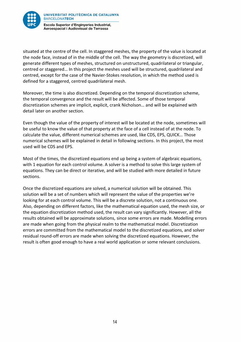
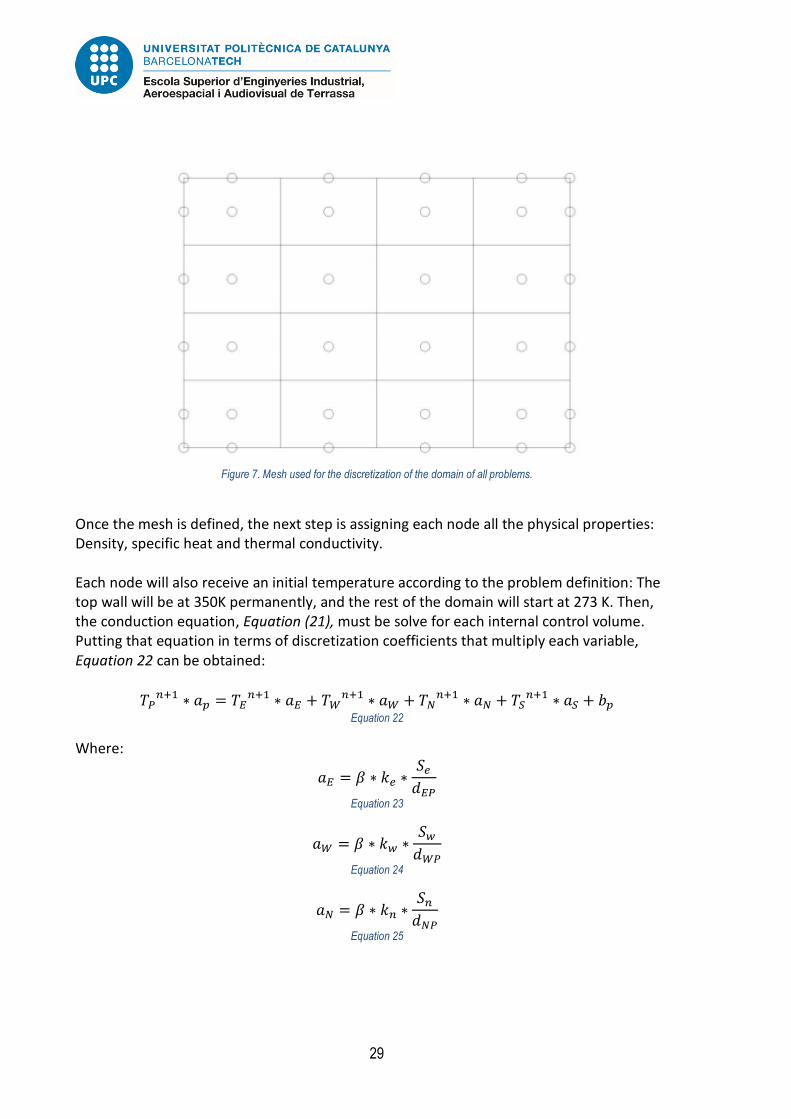
Figure 7. Mesh used for the discretization of the domain of all problems.

Once the mesh is defined, the next step is assigning each node all the physical properties: Density, specific heat and thermal conductivity. Each node will also receive an initial temperature according to the problem definition: The top wall will be at 350K permanently, and the rest of the domain will start at 273 K. Then, the conduction equation, Equation (21), must be solve for each internal control volume. Putting that equation in terms of discretization coefficients that multiply each variable, Equation 22 can be obtained:

𝑇𝑃𝑛+1 ∗ 𝑎𝑝 = 𝑇𝐸

𝑛+1 ∗ 𝑎𝐸 + 𝑇𝑊𝑛+1 ∗ 𝑎𝑊 + 𝑇𝑁

𝑛+1 ∗ 𝑎𝑁 + 𝑇𝑆𝑛+1 ∗ 𝑎𝑆 + 𝑏𝑝

Equation 22

Where:

𝑎𝐸 = 𝛽 ∗ 𝑘𝑒 ∗𝑆𝑒

𝑑𝐸𝑃

Equation 23

𝑎𝑊 = 𝛽 ∗ 𝑘𝑤 ∗𝑆𝑤

𝑑𝑊𝑃

Equation 24

𝑎𝑁 = 𝛽 ∗ 𝑘𝑛 ∗𝑆𝑛

𝑑𝑁𝑃

Equation 25

30

𝑎𝑆 = 𝛽 ∗ 𝑘𝑠 ∗𝑆𝑠

𝑑𝑆𝑃

Equation 26

𝑎𝑃 = 𝑎𝐸 + 𝑎𝑊 + 𝑎𝑁 + 𝑎𝑆 +𝜌 ∗ 𝐶𝑝 ∗ 𝑉

∆𝑡

Equation 27

𝑏𝑃 =𝜌 ∗ 𝐶𝑝 ∗ 𝑉 ∗ 𝑇𝑛

∆𝑡+ (1 − 𝛽) ∗ ∑ 𝑝

Equation 28

Where ∑ 𝑝is the sum of all the heat fluxes going through the faces of the control volume P

in instant ‘n’. This discretized equation obtained taking into account that there are no heat generated by intern sources, but the implementation of this term would be easy. However, since in our current case of study there are no intern sources of heat, those terms will be ignored. The thermal conductivity, 𝑘, at the faces is not defined, is defined for the nodes. To obtain the thermal conductivity at the face, a normal reasoning would be to just do the arithmetic mean between the thermal conductivities of the two nodes the face is in between. However, this can lead to huge errors in case the two nodes belong to different materials. To avoid that, the harmonic mean is used to calculate the thermal conductivity at the faces. Equation 29 shows the harmonic mean of the thermal conductivity for face ‘e’.

𝑘𝑒 =𝑑𝑃𝐸

𝑑𝑃𝑒

𝑘𝑃+

𝑑𝑒𝐸

𝑘𝐸

Equation 29

The same equation changing sub index can be used for the other faces. The boundary conditons will impose the temperature or a way to calculate the temperatures at the boundary nodes. In this case, there are three types of boundary conditions: Adiabatic wall, free convection wall and fixed temperature wall.

- In the fixed temperature wall, temperature will remain constant. In terms of the

discretization coefficients, 𝑎𝑝 = 1 and 𝑏𝑝 = 𝑇𝑡𝑜𝑝, and all the other coefficients will be

0. Tfix is the temperature which the wall has established.

31

- In the free convection wall, the conduction heat at the wall will be equalled to the

convection heat with air. Equation (X) shows this equality for the left free convection

wall, but the equation can easily be extrapolated for the west free convection wall.

𝑐𝑜𝑛𝑣 = 𝑐𝑜𝑛𝑑 = −𝑘 ∗𝑇𝐸 − 𝑇𝑃

𝑑𝐸𝑃= 𝛼 ∗ (𝑇𝑃 − 𝑇𝑒𝑥𝑡)

Equation 30

- In the adiabatic wall, the temperature of the node on the wall will be equalled to the

temperature of the closest internal node. In terms of the discretization coefficients,

supposing the south adiabatic wall,𝑎𝑝 = 1, 𝑎𝑛 = 1 and the rest of discretization

coefficients will be 0. That way, the temperature of node P, belonging to the

boundary south wall, will be equal to the temperature of node N, an interior node

just above node P.

Now that the heat conduction equation is defined for every node of the domain, a solver must obtain the temperature on all the nodes, solving the heat conduction equation. For this case, a Gauss-Seidel solver has been implemented, because of the simplicity of his implementation. Once the temperature of the ‘n+1’ instant of time is obtained through the resolution of Equation 22 with the Gauss-Seidel solver, the temperature just calculated, ‘n+1’, and the temperature of the last instant of time calculated, ‘n’, are compared. Each node’s temperature of both instants of times is compared, and the highest difference among them is obtained. If that difference is lower than a certain convergence value, call it 𝜀, usually a low number, the steady state is achieved and the calculation ends. However, if the maximum difference is higher than the convergence criteria another iteration of time is needed. The temperature of ‘n+1’ is now assigned to the temperature of ‘n’, and the necessary discretization coefficients are recalculated, in order to solve again the heat conduction equation. Time iterations are done until the convergence criteria is fulfilled, when the stationary state is accomplished. The resolution scheme is presented in Figure 8.

32

Figure 8. Resolution scheme for the 2D heat conduction case

33

3.2.5 RESULTS AND CONCLUSIONS

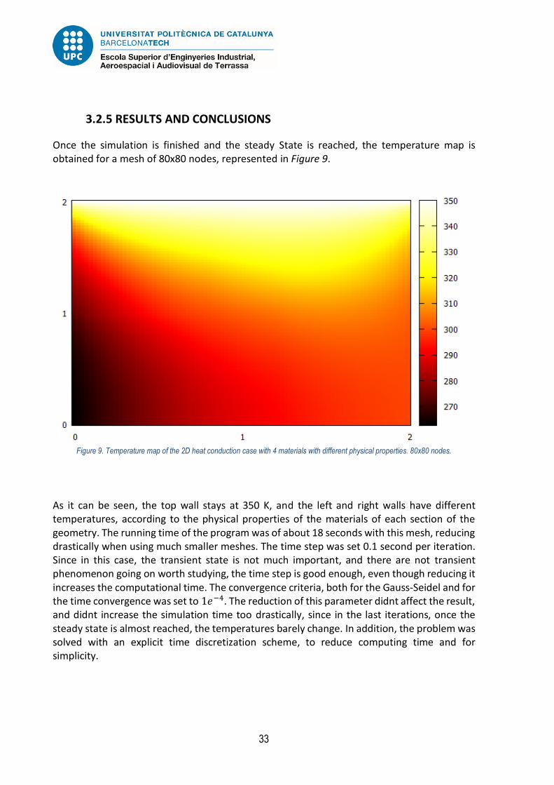
Once the simulation is finished and the steady State is reached, the temperature map is obtained for a mesh of 80x80 nodes, represented in Figure 9.

Figure 9. Temperature map of the 2D heat conduction case with 4 materials with different physical properties. 80x80 nodes.

As it can be seen, the top wall stays at 350 K, and the left and right walls have different temperatures, according to the physical properties of the materials of each section of the geometry. The running time of the program was of about 18 seconds with this mesh, reducing drastically when using much smaller meshes. The time step was set 0.1 second per iteration. Since in this case, the transient state is not much important, and there are not transient phenomenon going on worth studying, the time step is good enough, even though reducing it increases the computational time. The convergence criteria, both for the Gauss-Seidel and for the time convergence was set to 1𝑒−4. The reduction of this parameter didnt affect the result, and didnt increase the simulation time too drastically, since in the last iterations, once the steady state is almost reached, the temperatures barely change. In addition, the problem was solved with an explicit time discretization scheme, to reduce computing time and for simplicity.

34

To verify that at least the code is not functioning wrong, all materials are set to the same physical properties, and the temperature of the air fluid in both sides are set to the same value, 300K. In this way, the problem should be symmetrical, as it’s shown in Figure 10.

Figure 10 Temperature map of the 2D heat conduction case, with 1 material. 80x80 nodes

Moreover, to verify the code, the 2D problem was simplified to a 1D problem, converting the top wall with fixed temperature into an adiabatic wall. This way, the problem is converted into a 1D case, which has an analytical solution. The 1D problem is the same problem, with the top and bottom walls adiabatic, and the right and left walls are exchanging heat with external air through convection. The analytical solution for a 1D steady state plane wall is:

𝑇 =−𝑞𝑣

2 ∗ 𝑘∗ 𝑥2 + 𝐶1𝑥 + 𝑐

Equation 31

And for the heat flow, derivation with respect to x:

𝑞𝑥 = 𝑞𝑣 ∗ 𝑥 − 𝑘 ∗ 𝐶1 Equation 32

Where 𝑇 is the temperature, 𝑞𝑣 are the internal heat sources, 𝑘 is thermal conductivity, 𝐶1 and 𝐶2 are integration constants, 𝑞 is the heat flow and 𝑥 is the distance.

35

Using similar data of the problem simulated, the left wall air will be set to 250 K and the right wall air will be set to 300 K. The heat transfer coefficient will also be assumed to be 360 𝑤

𝑚2𝐾⁄ . Assuming one material, with constant physical properties, the conduction heat flux

through the left wall must be equal to the convection heat flow. Using this condition:

𝛼 ∗ (250 − 𝑇1) = 𝑞𝑥 Equation 33

For the right wall:

𝛼 ∗ (300 − 𝑇2) = 𝑞𝑥 Equation 34

Being 𝑇1 and 𝑇2 the temperatures and left and right walls respectively. Using the heat flow equation, and taking into account that the internal sources are 0:

𝑞𝑥 = −𝑘 ∗ 𝐶1 Equation 35

Using the temperature distribution equation, for the left wall, 𝑥 = 0, 𝑇 = 𝑇1

𝑇1 = 𝐶2 Equation 36

And for the right wall, 𝑥 = 𝐿 = 2 and 𝑇 = 𝑇2:

𝑇2 = +𝐶1𝐿 + 𝑇1 Equation 37

Isolating 𝐶1:

𝐶1 =𝑇2 − 𝑇1

𝐿

Equation 38

Now, both heat flows must be equal. Also, using 𝑘 = 200, Equations 39 and 40 can be written:

360 ∗ (250 − 𝑇1) = −200 ∗𝑇2 − 𝑇1

𝐿

Equation 39

36

360 ∗ (300 − 𝑇2) = −20 ∗𝑇2 − 𝑇1

2

Equation 40

This way, a system of 2 equations and 2 unknowns is formed, and both 𝑇1 and 𝑇2 can be obtained. Then 𝐶1 and 𝐶2 can be also calculated and the temperature distribution equation will be known. Solving, 𝑇1 = 258.9 and 𝑇2 = 291. Then the temperature distribution will follow Equation 41.

𝑇(𝑥) = 16.1𝑥 + 258.9 Equation 41

The simulation temperature map using the data for the analytical solution and using a mesh of 80x80 nodes is shown in Figure 11.

Figure 11. Temperature map of the 1D heat conduction case with analytical solution. 80x80 nodes.

Which now, plotting the analytical temperature distribution and comparing with the simulated distribution, Figure 12 is obtained:

37

Figure 12. Comparison between the temperatures of the numerical simulation and the analytical solution of the 1D heat conduction case

Where f(x) is the analytical solution, using Equation 41 and ‘simulation.txt’ is the simulated result. As it can be seen, both results are quite similar. The small differences are probably due to numerical errors, always present when doing a numerical simulation. However, the results can be considered equal and the validity of the code is confirmed.

3.2.6 PARALELIZED CASE: 1D TRANSISTENT PROBLEM

For the case of heat conduction, an extra study was made. A 1D transient heat conduction problem was programed, but this time for the processors to work in parallel, which should considerably reduce the computational time for the resolution of the problem. The case studied is the same that was used to verify the functionality of the code, a top and bottom adiabatic wall, and the two side walls surrounded by air, exchanging heat by natural convection. The physical problem was not the main focus of this study, but the study of the influence of using multiple processors to solve the problem, and the things that have to be taken into account when parallelizing a heat conduction problem. Each processor will be assigned a certain part of the global domain, and will calculate the temperature for those nodes using the same heat conduction, Equation 21. This work split is done by rows, to avoid complexity. For example, if the domain has a mesh of 10x10 nodes, and 5 processors are being used, each processor will compute the calculation’s needed for two rows of nodes in the Y direction. However, in order to compute the temperature in a

38

node, the temperatures of the boundary nodes are needed, and if each processor only calculates the nodes that the work-split has given to him, that processor will not have some of the boundary nodes needed in order to calculate the temperature in all its domain. To solve this problem, the halos are needed. Halos are fictitious nodes, added in the boundaries of each processors domain which contain the temperature of the nodes that are needed for the currently calculating processor to be able to compute the temperatures without any missing information. The halo implementation was the hardest part of the programming, because of the need of multiple processors to send and receive information at the same time. In addition, by doing this program, the impact of using multiple processors was observed. The computational time decreased more or less linearly with the number of processors used. For example, for a 30x30 nodes mesh, 0.8 seconds were needed for 1 processor. Using two processors, the time decreased to half this 0.8 value approximately, and so on until using all the processors of the computer running the simulation. Overall, using more processors clearly helps when talking about computational time, and for big simulations that are run in supercomputers, this is completely necessary. However, for academicals purposes, the results obtained using only 1 processor, with meshes without high resolution are good enough, even though academically is also very illustrating to program oneself a parallelized code: adds extra difficulty, but the fruits of the work also are reflected on the computational time.

39

3.3 POTENTIAL FLOW

The potential flow describes a velocity field as the gradient of a scalar function, called the velocity potential. There are two approaches to the potential flow: based on stream functions and based on velocity potential. The potential flow based on stream functions can be used for non-rotational and rotational flows, but is limited to steady 2D flows. The velocity potential flow can be used only for non-rotational flows, however it can be used for 3D unsteady cases. In this project, the main focus will be set on the stream function based potential flow. In this section, a 2D potential flow problem will be solved, and the solution will be validated through the comparison with the analytical solution of the problem.

3.3.1 POTENTIAL FLOW EQUATIONS

The velocities of a stream function are defined in Equations 42 and 43.

𝑣𝑥 =𝜌𝑜

𝜌∗

𝜕𝜓

𝜕𝑦

Equation 42

𝑣𝑦 = −𝜌𝑜

𝜌∗

𝜕𝜓

𝜕𝑥

Equation 43

Where 𝑣𝑥 and 𝑣𝑦 are the velocities in the x and y direction, 𝜌 is the density, 𝜌𝑜 is the density

at reference conditions and 𝜓 is the stream function. The equation for the stream function can be obtained, if the vorticity is known:

𝜕

𝜕𝑥(

𝜌𝑜

𝜌∗

𝜕𝜓

𝜕𝑥) +

𝜕

𝜕𝑦(

𝜌𝑜

𝜌∗

𝜕𝜓

𝜕𝑦) = 𝜔𝑧

Equation 44

Where 𝜔𝑧 is the vorticity. From the definition of circulation, Г:

Г = ∮ ∗ 𝑑𝑙𝐶

Equation 45

And using stokes theorem, Equation 46.

40

∫ (∇ 𝑥 ) ∗ 𝑑𝑆 =𝑆

∮ ∗ 𝑑𝑙𝐶

Equation 46

Now, assuming non-rotational flow (∇ 𝑥 = 0):

Г = ∮ ∗ 𝑑𝑙𝐶

= 0

Equation 47

3.3.2 EQUATIONS DISCRETIZATION

Integrating equation(X) for a control volume (see figure X), the following expression for the circulation can be obtained:

Г = 𝑣𝑦𝑒 ∗ ∆𝑦 − 𝑣𝑥𝑛 ∗ ∆𝑥 − 𝑣𝑦𝑤 ∗ ∆𝑦 + 𝑣𝑥𝑠 ∗ ∆𝑥 = 0 Equation 48

Figure 13. Scheme of the velocities nomenclature of a control volume for the potential flow resolution.

41

Now, simplifying the derivatives in the Equations 42 and 43 of the potential flow velocitites:

𝑣𝑦𝑒 =𝜌𝑜

𝜌∗

𝜓𝐸 − 𝜓𝑃

𝑑𝐸𝑃

Equation 49

𝑣𝑥𝑛 = −𝜌𝑜

𝜌∗

𝜓𝑁 − 𝜓𝑃

𝑑𝑁𝑃

Equation 50

𝑣𝑦𝑤 =𝜌𝑜

𝜌∗

𝜓𝑃 − 𝜓𝑊

𝑑𝑊𝑃

Equation 51

𝑣𝑥𝑠 = −𝜌𝑜

𝜌∗

𝜓𝑃 − 𝜓𝑆

𝑑𝑆𝑃

Equation 52

Then, replacing Equations 49, 50, 51 and 52 in Equation 48, the following expression can be obtained:

−𝜌𝑜

𝜌∗

𝜓𝐸 − 𝜓𝑃

𝑑𝐸𝑃∗ ∆𝑦 −

𝜌𝑜

𝜌∗

𝜓𝑁 − 𝜓𝑃

𝑑𝑁𝑃∗ ∆𝑥 +

𝜌𝑜

𝜌∗

𝜓𝑃 − 𝜓𝑊

𝑑𝑊𝑃∗ ∆𝑦 +

𝜌𝑜

𝜌∗

𝜓𝑃 − 𝜓𝑆

𝑑𝑆𝑃∗ ∆𝑥 = 0

Equation 53

Where 𝑑𝑖𝑗 are the distances between the nodes the sub index indicates, ∆𝑦 is the heigth of

the control volume, ∆𝑥 is the longitude of the control volume, 𝜓 is the stream function at the node the sub index indicates, ρ is the density and 𝜌𝑜 is the density at reference conditions.

3.3.3 PROBLEM DEFINITION

The potential flow problem that will be solved will be the flow around a static cylinder inside a conduct, assuming incompressible flow. The analytical solution of this problem is known, so the comparison of the numerical and the analytical results can be easily done. The domain will be a conduct of height 𝐻 20m and longitude 𝐿 of 20m. The cylinder, of radius 2.5m, will be located at the middle of the domain. However, the symmetry of this problem will be used to make the problem simpler. Only the upper half of the domain will be resolved, since the lower half will be exactly the same, due to the symmetry of the problem. Figure 14 is a visual representation of the problem to be solved.

42

Figure 14. Scheme of the potential flow problem to be solved.

This is a steady problem, so no temporal discretization will be needed. The stream functions at the left boundaries are known, and expressed in Table 2.

Wall Top Bottom Left Right

𝝍 𝜓 = 𝐻 ∗ 𝑣𝑜 𝜓 = 0 𝜓 = 𝑦 ∗ 𝑣𝑜 𝑑𝜓

𝑑𝑦= 0

Table 2. Boundary conditions values for the flow around a cylinder potential flow problem

Where 𝑦 is the height of the node and 𝑣𝑜 is the inlet velocity. The inlet velocity will be set to 10 𝑚 𝑠⁄ , and the pressure and temperature values at the inlet, which will be used as reference values, will be set to 1𝑒5 Pa and 350K respectively. Using air as the fluid that is going around the cylinder, 𝑟 = 287 using ideal gases law, the pressure can

be obtained, and its value is 0.9956 𝑘𝑔

𝑚3⁄ . In addition, in order to calculate the

temperatures later on, a specific heat value will be set to 1000 𝐽

𝑘𝑔 ∗ 𝐾⁄ .


With the problem defined and the equation that has to be solved discretized, the resolution of the problem can commence. The first step is to create a mesh. The mesh will be the same kind used for the 2D transient heat conduction case (see Figure 7). With the mesh defined and the physical properties defined and assigned a number, each node will receive an initial guess of the stream function value. For example, all the interior nodes will be set to 10, except the boundary nodes, that the value set for the stream function can be seen at section 3.2.3, where the boundary conditions are explained.

43

The discretized equation that has to be solved, Equation 53, will now be rearranged to put the equation in terms of the discretization coefficients to obtain Equation 54.

𝜓𝑃 ∗ 𝑎𝑝 = 𝜓𝐸 ∗ 𝑎𝐸 + 𝜓𝑊 ∗ 𝑎𝑊 + 𝜓𝑁 ∗ 𝑎𝑁 + 𝜓𝑆 ∗ 𝑎𝑆 + 𝑏𝑝 Equation 54

Where

𝑎𝐸 =𝜌𝑜 ∗ ∆𝑦

𝜌𝑒 ∗ 𝑑𝑃𝐸

Equation 55

𝑎𝑊 =𝜌𝑜 ∗ ∆𝑦

𝜌𝑤 ∗ 𝑑𝑃𝑊

Equation 56

𝑎𝑁 =𝜌𝑜 ∗ ∆𝑥

𝜌𝑛 ∗ 𝑑𝑃𝑁

Equation 57

𝑎𝑆 =𝜌𝑜 ∗ ∆𝑥

𝜌𝑠 ∗ 𝑑𝑃𝑆

Equation 58

𝑎𝑃 = 𝑎𝐸 + 𝑎𝑊 + 𝑎𝑁 + 𝑎𝑆 Equation 59

𝑏𝑝 = 0 Equation 60

But since this is an incompressible regime, with 𝑣𝑜 = 10𝑚/𝑠, the density at the faces and the reference densities will cancel out. Equation 54 will have to be solved for every interior node that is not a solid node. Since in this case the study is the flow around a solid, the nodes which are located in the fluid and the nodes located at the solid must be identified. Once the nodes that belong to each matter state are identified, the nodes which are on the fluid will have its density set to the value of the inlet density (incompressible flow), and the nodes which belong to a solid will have its density set to 0. Then, when calculating, for example, the densities division in face ‘e’, the harmonic mean will be done instead:

𝜌𝑜

𝜌𝑒=

𝑑𝑃𝐸

𝑑𝑃𝑒

𝜌𝑜/𝜌𝑃+

𝑑𝐸𝑒

𝜌𝑜/𝜌𝐸

Equation 61

44

In case of both nodes P and E being fluid, the division will just be averaged. In case of both nodes being solid, the division value will be 0, and in case of solid-fluid interaction, the expression will be:

𝜌𝑜

𝜌𝑒= (𝜌𝑜/𝜌𝐸) ∗ (𝑑𝑃𝐸/𝑑𝐸𝑒)

Equation 62

In this way, the fluid-solid interaction will be taken into account, and will be reflected in the discretization coefficients. This methodology is known as the blocking-off method. Similarly to the 2D heat conduction case, in the nodes where the stream functions are fixed, the value of some discretization coeficients will be special:

- For the left boundary, 𝑎𝑝 = 1 and 𝑏𝑝 = 𝑦 ∗ 𝑣𝑜

- For the top wall, 𝑎𝑝 = 1 and 𝑏𝑝 = 𝐻 ∗ 𝑣𝑜

- For the bottom wall, 𝑎𝑝 = 1 and 𝑏𝑝 = 0, which will set the value of the stream

function to 0

- For the right wall, 𝑎𝑝 = 1 and 𝑎𝑊 = 1, which will set the value of the stream function

to the stream function at the node at the left.

The discretization coefficients not specified for the boundary conditions will be set to 0. Now that the discretization coefficients are defined for every node, the equation can be solved. Gauss-Seidel solver was used to resolve the discretized Equation 54, due to the simplicity of implementation. The solver will obtain the stream function in every node of the domain, solving the potential flow equation. Since this is an incompressible case and steady, once the stream function are known, the only thing left to do is to calculate the velocities and the temperatures and pressures at each node. Velocities for each control volume’s face can be calculated with Equations 49, 50, 51 and 52. Once the velocities at the faces are known, they are arithmetically averaged to obtain the value at the node:

𝑣𝑥𝑃 =𝑣𝑥𝑛 + 𝑣𝑥𝑠

2

Equation 63

𝑣𝑦𝑃 =𝑣𝑦𝑒 + 𝑣𝑦𝑤

2

Equation 64

Now, the total velocity of each node is calculated with Equation 65.

45

𝑣𝑝 = √𝑣𝑥𝑝2 + 𝑣𝑦𝑝

2

Equation 65

Then, since total energy is conserved, temperature can be calculated:

ℎ𝑜 + 𝑒𝑘𝑜 = ℎ𝑝 + 𝑒𝑘𝑝 Equation 66

Where ℎ is the enthalpy and 𝑒𝑘is the kinetical energy. Then, using the definition of enthalpy and kinetical energy:

𝑇𝑃 = 𝑇𝑜 + (𝑣𝑜2 − 𝑣𝑝

2)/(2 ∗ 𝐶𝑝) Equation 67

Where 𝑇𝑃 is the temperature at the node, 𝑇𝑜 is the reference temperature, 𝑣𝑜 is the reference velocity, 𝑣𝑝 is the velocity at the node, and 𝐶𝑝 is the specific heat.

To calculate the pressure, the isentropic relation can be used:

𝑝𝑝 = 𝑝𝑜 ∗ (𝑇𝑝

𝑇𝑜)

𝛾𝛾−1

Equation 68

Where 𝑝𝑝 is the pressure at the node, 𝑝𝑜 is the reference pressure, 𝑇𝑝 is the temperature at

the node, 𝑇𝑜 is the reference temperature and 𝛾 is the heat capacity ratio, 1,4 for air suposing it a diatomic gas. Density could then be calculated using the ideal gas equation, but since the inflow velocity is so low, the fluid can be assumed incompressible and the values will differ so little from the original reference density, and the density in each node imposed at the beginning. In case the flow was compressible, after calculating the density, the recently calculated density and the initial one would be compared. Then, if the maximum difference of those two values among all the nodes of the domain would be higher than a certain convergence criteria, another iteration would be done, taking as the new initial density the just recently calculated, and so on until the convergence criteria was fulfilled. The resolution algorithm can be seen at Figure 15.

46

Figure 15. Resolution scheme of the potential flow problem.

47


Once the simulation is completed, the module of the velocity map is obtained, represented in Figure 16. The mesh used was a 100 x 100 nodes mesh. The stream function plot can be seen in Figure 17.

Figure 16. Velocity module field for the flow around a cylinder, using 100x100 nodes.

48

Figure 17. Stream function map of the flow around a cylinder case, using 100x100 nodes.

The computational time was quite short compared to the 2D heat transfer case, it lasted around 4 seconds. The reason behind is because the problem is steady, and incompressible, and the only iterations to be done are the ones for the Gauss-Seidel solver, not any time iterations or density calculation iterations. As we can see, the points where the velocity is 0 are the solid nodes, where the cylinder is. Velocity increases to almost double the inflow value when passing the cylinder, and then decreases again to the inflow value when far away from the cylinder. Also, the stagnation points at the left and right of the cylinder can be seen. In those points, the velocity decreases to 0 or almost 0. In order to verify the validity of this results, the analytical solution and the numerical will be compared. The analytical solution for the stream function value will be evaluated, using Equation 69.

𝜓 = (𝑟 −𝑅2

𝑟) ∗ 𝑈 ∗ sin (𝜃)

Equation 69

Where r is the distance from the centre of the cylinder, 𝑅 is the cylinder radius, 𝑈 is the inflow velocity and 𝜃 is the radial velocity. The results at 𝑟 = 𝑅 for different angles will be compared.

49

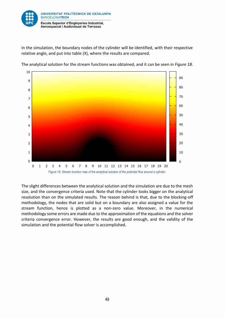
In the simulation, the boundary nodes of the cylinder will be identified, with their respective relative angle, and put into table (X), where the results are compared. The analytical solution for the stream functions was obtained, and it can be seen in Figure 18.

Figure 18. Stream function map of the analytical solution of the potential flow around a cylinder.

The slight differences between the analytical solution and the simulation are due to the mesh size, and the convergence criteria used. Note that the cylinder looks bigger on the analytical resolution than on the simulated results. The reason behind is that, due to the blocking-off methodology, the nodes that are solid but on a boundary are also assigned a value for the stream function, hence is plotted as a non-zero value. Moreover, in the numerical methodology some errors are made due to the approximation of the equations and the solver criteria convergence error. However, the results are good enough, and the validity of the simulation and the potential flow solver is accomplished.

50

3.4 CONVECTION-DIFFUSION

The convection diffusion equation describe physical phenomena where particles or energy are transferred in a physical domain thanks to two processes: convection and diffusion. The generic convection diffusion equation will find a solution for a generic variable, Ф. The resolution of the generic convection diffusion equation is the last step before resolving Naiver-stokes equations, because the Navier-Stokes equations are convection diffusion equations. In this section, a generic convection-diffusion problem will be solved. The solution obtained will be compared with a benchmark solution given by the CTTC, which will validate the program created.

3.4.1 CONVECTION-DIFFUSION EQUATIONS

The generic convection diffusion equation can be written as:

𝜕(𝜌 ∗ Ф)

𝜕𝑡+ ∇ ∗ (𝜌Ф) = ∇ ∗ (ГФ∇Ф) + 𝑠Ф

Equation 70

Where ρ is the density, Ф is a generic variable, is the velocity vector, ГФ is the diffusion coeficient and 𝑠Ф is the source term. Using the mass conservation equation (X), the convection diffusion equation can be transformed to:

𝜕𝜌

𝜕𝑡+ ∇ ∗ (𝜌) = 0

Equation 71

𝜕(𝜌 ∗ Ф)

𝜕𝑡+ 𝜌 ∗ ∇Ф = ∇ ∗ (ГФ∇Ф) + 𝑠Ф

Equation 72

When resolving the Navier-Stokes equations, the generic variable, source term and diffusion coefficients will take the role of different variables. In Table 3, this variables for each equation can be seen.

Equation Ф ГФ 𝒔Ф

Mass 1 0 0

Momentum 𝜇 ∇ ∗ (𝜏 − 𝜇∇) − ∇𝑝 + 𝜌 Energy T 𝑘

𝐶𝑣

1

𝐶𝑣(−∇ ∗ 𝑞𝑅 − 𝑝∇ ∗ + 𝜏 ∗ ∇

Table 3. Values of different variable parameters to convert the generic convection-diffusion equation into the Navier-Stokes equations

51

3.4.2 TEMPORAL AND SPATIAL DISCRETIZATION

Witting the continuity equation in integral form, Equation 73 is obtained:

𝜕

𝜕𝑡∫ 𝜌𝑑𝑉 + ∫ 𝜌 ∗ 𝑑𝑆 = 0

𝑆𝑓𝑉

Equation 73

Approximating the Surface integral for the mass flows across each face and the volume integral for the total volume of a control volume, and finally integrating with time the following expression can be obtained:

𝑉 ∫𝜕𝜌

𝜕𝑡𝑑𝑡 +

𝑡+∆𝑡

𝑡

∫ (𝑒 − 𝑤 + 𝑛 − 𝑠)𝑑𝑡 = 0𝑡+∆𝑡

𝑡

Equation 74

Where 𝑉 is the volume, 𝜌 is the density, and 𝑖 are the mass flows across each face. Integrating in time, with a fully implicit scheme, the following continuity equation discretized can be obtained:

(𝜌𝑛+1 − 𝜌𝑛) ∗ 𝑉

∆𝑡+ 𝑒

𝑛+1 − 𝑤𝑛+1 + 𝑛

𝑛+1 − 𝑠𝑛+1 = 0

Equation 75

From now on, since implicit scheme will be used, the super index 𝑋𝑛+1 will be skipped, and the variables at the instant ‘n’ will remain using the super index 𝑋𝑛. Now, discretizing each term of the convection diffusion equation, Equation 72, the discretized terms can be obtained, reprsesented in Equations 76, 77, 78 and 79.

∫ ∫𝜕(𝜌 ∗ Ф)

𝜕𝑡𝑑𝑉𝑑𝑡 = 𝑉 ∗ (𝜌 ∗ Ф𝑃 − 𝜌𝑛 ∗ Ф𝑃

𝑛)𝑉

𝑡+∆𝑡

𝑡

Equation 76

∫ ∫ ∇ · (𝜌Ф)𝑑𝑉𝑑𝑡 = (𝑒 ∗ Ф𝑒𝑉

𝑡+∆𝑡

𝑡

− 𝑤 ∗ Ф𝑤 + 𝑛 ∗ Ф𝑛 − 𝑠 ∗ Ф𝑠)∆𝑡

Equation 77

52

∫ ∫ ∇ ∗ (ГФ∇Ф)𝑑𝑉𝑑𝑡𝑉

=𝑡+∆𝑡

𝑡

(Г𝑒

Ф𝐸 − Ф𝑃

𝑑𝑃𝐸𝑆𝑒 − Г𝑤

Ф𝑃 − Ф𝑊

𝑑𝑃𝑊𝑆𝑤 + Г𝑛

Ф𝑁 − Ф𝑃

𝑑𝑃𝑁𝑆𝑛

− Г𝑠

Ф𝑃 − Ф𝑆

𝑑𝑃𝑆𝑆𝑠) ∗ ∆𝑡

Equation 78

∫ ∫ 𝑠Ф𝑑𝑉𝑑𝑡 = (𝑆𝐶Ф + 𝑆𝑃

Ф ∗ Ф𝑃) ∗ ∆𝑡𝑉

𝑡+∆𝑡

𝑡

Equation 79

From now on, thinking about the problem that will be solved, that will have no source term; the source term will be equalled to 0. Grouping each discretized term, the generic convection diffusion equation discretized can be seen at Equation 80.

𝑉 ∗ (𝜌 ∗ Ф𝑃 − 𝜌𝑛 ∗ Ф𝑃𝑛)

∆𝑡+ 𝑒 ∗ Ф𝑒 − 𝑤 ∗ Ф𝑤 + 𝑛 ∗ Ф𝑛 − 𝑠 ∗ Ф𝑠

= 𝐷𝑒(Ф𝐸 − Ф𝑃) − 𝐷𝑤(Ф𝑃 − Ф𝑊) + 𝐷𝑛(Ф𝑁 − Ф𝑃) − 𝐷𝑠(Ф𝑃 − Ф𝑆) Equation 80

Where

𝐷𝑒 =Г𝑒𝑆𝑒

𝑑𝑃𝐸

Equation 81

𝐷𝑤 =Г𝑤𝑆𝑤

𝑑𝑃𝑊

Equation 82

𝐷𝑛 =Г𝑛𝑆𝑛

𝑑𝑃𝑁

Equation 83

𝐷𝑠 =Г𝑠𝑆𝑠

𝑑𝑃𝑆

Equation 84

Using the continuity equation, the generic convection diffusion discretized equation can be transformed into Equation 85.

53

𝑉 ∗ (𝜌 ∗ Ф𝑃 − 𝜌𝑛 ∗ Ф𝑃𝑛)

∆𝑡+ 𝑒(Ф𝑒 − Ф𝑃) − 𝑤(Ф𝑤 − Ф𝑃) + 𝑛(Ф𝑛 − Ф𝑃)

− 𝑠(Ф𝑠 − Ф𝑃)= 𝐷𝑒(Ф𝐸 − Ф𝑃) − 𝐷𝑤(Ф𝑃 − Ф𝑊) + 𝐷𝑛(Ф𝑁 − Ф𝑃) − 𝐷𝑠(Ф𝑃 − Ф𝑆)

Equation 85

This implicit discretization of the generic convection diffusion equation is a second order approximation. Until now, the values of the main variable of study, like velocities or temperatures, only were needed at the nodes, or they could be easily calculated at the faces. However, in this equation, the values of Ф are needed for the resolution of the equation. To calculate those, numerical schemes for interpolation will be needed (see section ....). Note that the obtaining of this equation was supposing constant physical properties in all the domain.


The convection diffusion problem that will be solved is the called Smith-Hutton problem. This problem consists in a rectangular geometry, with an inlet at the bottom left and an outlet at the bottom right. The flow will follow a solenoidal path, going from the bottom left, the inlet of the flow, to the bottom right, the outlet of the flow. A visual representation of the problem can be seen at Figure 19.

Figure 19. Smith-Hutton problem definition scheme.

54

The velocity field will be given by Equations 86 and 87. The values of the variable of study Ф will also be given in the boundaries. Those values can be seen on Table 4.

𝑣𝑥 = 2 ∗ 𝑦(1 − 𝑥2) Equation 86

𝑣𝑦 = −2 ∗ 𝑥(1 − 𝑦2)

Equation 87

Where 𝑥 and 𝑦 are the horizontal and vertical position respectively, and 𝑣𝑥 and 𝑣𝑦 are the

horizontal and vertical velocities respectively.

Location Inlet (-1, 0 in x) Outlet(0, 1) in x

Left boundary Rigth boundary

Top boundary

Ф 1 + tanh [10(2𝑥+ 1)]

𝜕Ф

𝜕𝑦= 0

1 − tanh (10) 1− tanh (10)

1− tanh (10)

Table 4. Boundary conditions for the Smith-Hutton problem.

Note that the velocity field fulfils the incompressibility condition, ∇ ∗ = 0. With the boundaries defined, the initial nodes have to also be set to an initial value for the resolution of the problem.


With the problem defined, a mesh has to be chosen. The same way that in the two past cases, the mesh used will be an structured, Cartesian, quadrilateral and node centred mesh, adding nodes at the boundaries for easier implementation of the boundary conditions (see Figure 7) With the mesh defined, physical properties are defined, such as the reference velocity, the density... Numerical variables are also defined, like the convergence criteria or the time step.

55

Each node will also be set to a certain initial Ф value, arbitrarily. In this case, for example was set to 1. The boundary nodes were set to the Ф indicated in Table 4. In addition, each node was also assigned a vertical velocity and horizontal velocity, which can be calculated with Equations 86 and 87. After that, the generic convection diffusion equation discretized must be solved. Rearranging the variables to have the equation in terms of the discretization coefficients that multiply each variable, Equation 88 can be obtained:

Ф𝑃𝑛+1 ∗ 𝑎𝑝 = Ф𝐸

𝑛+1 ∗ 𝑎𝐸 + Ф𝑊𝑛+1 ∗ 𝑎𝑊 + Ф𝑁

𝑛+1 ∗ Ф𝑁 + Ф𝑆𝑛+1 ∗ 𝑎𝑆 + 𝑏𝑝

Equation 88

Where: 𝑎𝐸 = 𝐷𝑒 ∗ 𝐴(|𝑃𝑒|) + max (−𝑒 , 0)

Equation 89

𝑎𝑊 = 𝐷𝑤 ∗ 𝐴(|𝑃𝑤|) + max(𝑤 , 0) Equation 90

𝑎𝑁 = 𝐷𝑛 ∗ 𝐴(|𝑃𝑛|) + max(−𝑛, 0) Equation 91

𝑎𝑆 = 𝐷𝑠 ∗ 𝐴(|𝑃𝑠|) + max (𝑠, 0)

Equation 92

The expression 𝐷𝑖, i=(e,w,n,s) can be found in Equations 81, 82, 83 and 84. The values of the mass fluxes can be easily calculated using Equations 93, 94, 95 and 96.

𝑒 = 𝜌 ∗ 𝑢𝑒 ∗ ∆𝑦 Equation 93

𝑤 = 𝜌 ∗ 𝑢𝑤 ∗ ∆𝑦 Equation 94

𝑛 = 𝜌 ∗ 𝑢𝑛 ∗ ∆𝑥 Equation 95

𝑠 = 𝜌 ∗ 𝑢𝑠 ∗ ∆𝑥 Equation 96

56

𝐴(|𝑃𝑠|) Is a parameter that will be defined by the numerical interpolation method used (see section .... for more information about numerical interpolation methods), and that will also depend on the Peclet number (Equation 97). The value of this parameter, as a function of the scheme chosen, can be found on Table 5.

NUMERICAL SCHEME 𝑨(|𝑷𝒔|)

UDS 1

CDS 1-0.5*|Pe|

HDS Max(0, 1-0.5*|Pe|)

EDS |Pe|/(e |Pe| − 1) Table 5. Values of 𝐴(|𝑃|) for the different numerical schemes as a function of the Peclet number

𝑃𝑒 =𝜌 ∗ 𝑢 ∗ 𝐿

Г

Equation 97

Where 𝜌 is the density, 𝑢 the velocity, 𝐿 is the characteristic longitude and Г is the diffusion coefficient. In this case, the EDS scheme was used, due to the simplicity of implementation, even though its only a first order approximation scheme. For the boundary conditions, for all the walls except for the right bottom wall, corresponding to the outlet, the Ф value is fixed. Then, to put that information in the discretization coefficients, 𝑎𝑝 = 1 and 𝑏𝑝 = Ф𝑓𝑖𝑥, where Ф𝑓𝑖𝑥 is

whatever Ф the wall is fixed at. For the outlet, the derivative of Ф is fixed to 0 in the ‘y’ direction. In terms of the discretization coefficients, that means 𝑎𝑝 = 1, 𝑎𝑁 = 1.

Now that every node has its discretization coefficients defined, the resolution using a Gauss-Seidel scheme can be done, which will allow obtaining Ф(n+1). Then, similarly to the other cases, the time convergence is checked. If each node’s Ф difference is lower than a certain numerical convergence criteria, the steady state is reached. However, if in some of the nodes the difference is bigger, another iteration is needed, and the Ф of ‘n+1’ is assigned to Ф of ‘n’, and another iteration of time will be done until the steady state is reached. The resolution algorithm for the Smith-Hutton problem can be seen in Figure 20.

57

Figure 20. Resolution scheme of the Smith-Hutton problem.


In this case, the results of the Smith-Hutton problem will be exposed for different values of 𝜌

Г⁄ , assuming reference velocity equal to 1 and height of the geometry equal to 1, in

international system units. If the reference velocity and the height are equal to 1, then 𝜌

Г⁄ =

𝑃𝑒.

𝜌Г⁄ = 𝑃𝑒 =

𝜌 ∗ 𝑢 ∗ 𝐿

Г=

𝜌 ∗ 1 ∗ 1

Г

Equation 98

58

𝝆Г⁄

10

10e3

10e6 Table 6. Different

𝜌Г⁄ values solved for the Smith-Hutton problem.

The CTTC proposes some reference results of the Ф value at the outlet. The comparison between the reference results and the numerically obtained ones will be done. That comparison can be seen at Table 7 . In all the simulations, the mesh used was a mesh of 200x100 nodes, with a convergence criteria of 1e-5 and a time step of 0.1 seconds per temporal iteration.

𝝆Г⁄ = 𝟏𝟎

𝝆Г⁄ = 𝟏𝟎𝟑

𝝆Г⁄ = 𝟏𝟎𝟔

x-Position Reference Simulated Reference Simulated Reference Simulated

0.0 1.989 1.892 2.000 2.000 2.000 2.000

0.1 1.402 1.388 1.9990 2.000 2.000 2.000

0.2 1.146 1.112 1.9997 1.999 2.000 2.000

0.3 0.946 0.933 1.9850 1.977 1.999 1.956

0.4 0.775 0.701 1.8410 1.712 1.964 1.821

0.5 0.621 0.598 0.9510 0.9120 1.000 0.920

0.6 0.480 0.425 0.1540 0.1430 0.036 0.021

0.7 0.349 0.332 0.0010 0.000 0.001 0.009

0.8 0.227 0.211 0.000 0.000 0.000 0.000

0.9 0.111 0.099 0.000 0.000 0.000 0.000

1 0 0.000 0.000 0.000 0.000 0.000 Table 7. Comparison of the reference and simulated results for the Smith-Hutton problem, for different

𝜌Г⁄ values

59

Figure 21. Comparison between reference and simulated results for the Smith-Hutton problem,

𝜌Г⁄ = 10


𝜌Г⁄ = 10𝑒3

0

0.5

1

1.5

2

2.5

0 0.2 0.4 0.6 0.8 1 1.2

Ф

x

𝝆⁄Г=𝟏𝟎 result comparison

Reference

Simulated

0

0.5

1

1.5

2

2.5

0 0.2 0.4 0.6 0.8 1 1.2

Ф

X

𝝆⁄Г=𝟏e3 result comparison

Reference

Simulated

60


𝜌Г⁄ = 10𝑒6

As Figures 21,22 and 23 show, the results of the simulation and the ones given by the CTTC are quite similar. The differences are probably due to mesh refinement, convergence criteria or numerical schemes differences between the simulation done in this project and the simulation made to obtain the reference results. However, seeing how small the differences are, it is acceptable to say that both results are almost equal, and the validity of the program seems correct. In Figures 24, 25 and 26, the Ф map can be seen for the three different values

of 𝜌

Г⁄ .

0

0.5

1

1.5

2

2.5

0 0.2 0.4 0.6 0.8 1 1.2

Ф

X

𝝆⁄Г=𝟏e6 result comparison

Reference

Simulated

61

Figure 24. Map of Ф for the Smith-Hutton problem, with

𝜌Г⁄ = 10


𝜌Г⁄ = 10𝑒3

62


𝜌Г⁄ = 10𝑒6

Observing the three figures above, it can be easily deduced than, the higher the 𝜌

Г⁄ ratio, the

smoother is the flux going from the inlet to the outlet. The smaller the ratio, the less symmetric the flow is. The simulations, using a mesh of 200x100 nodes, took more time the lower the 𝜌

Г⁄ ratio, going from around 10 minutes less than 3 minutes. Note also that the difference

between 𝜌

Г⁄ = 10𝑒3 and 10𝑒3 is very little. Increasing the ratio makes increase the

convective terms be more important than the diffusive. All in all, comparing the results obtained by the simulation run in this project, it’s safe to say that this case was well programmed, and the results obtained are for sure correct.

63

3.5 NAVIER-STOKES

The Navier-Stokes equations are a set of non-linear partial derivative equations that describe the movement of a Newtonian fluid. The atmosphere dynamics, the flow around an air foil or the ocean water movements are all ruled by this equations. However, like most non-linear partial derivative equations, this equations don’t have a analytical solution, so the only way to solve them without oversimplifying the problem is using numerical simulations. This equations can be obtained applying conservation principals of mechanics and thermodynamics to a control fluid volume. In this section, a 2D fluid dynamics problem will be solved by resolving the Navier-Stokes equations, using the fractional step method. The results obtained in the simulations will be compared with reference results given by the CTTC, which will be the criteria to know if the code programmed is correct or not.

3.5.1 THE NAVIER-STOKES EQUATIONS

The Navier-Stokes equations are 5 equations: The mass conservation equation, the three momentum conservation equaitons,one for each spatial dimension, and the energy conservation equation. Writing them in integral form, Equations 99, 100 and 101. are obtained:

𝑑

𝑑𝑡∫ 𝜌 ∗ 𝑑𝑉 + ∫ 𝜌 ∗ ∗ ∗ 𝑑𝑆 = 0

𝑆𝑉𝑜𝑙

Equation 99

𝑑

𝑑𝑡∫ 𝜌 ∗ 𝑑𝑉 + ∫ 𝜌 ∗ 𝑑𝑆 = ∫ 𝑓𝑛𝑑𝑆 + ∫ ∗ 𝜌𝑑𝑉

𝑉𝑜𝑙𝑆𝑆𝑉𝑜𝑙

Equation 100

𝑑

𝑑𝑡∫ (𝑢 + 𝑒𝑘)𝜌 ∗ 𝑑𝑉

𝑉𝑜𝑙

+ ∫ (𝑢 + 𝑒𝑘)𝜌 ∗ 𝑑𝑆 = − ∫ ∗ 𝑑𝑆𝑆

∫ 𝑣 ∗ 𝑓𝑛𝑑𝑆 + ∫ 𝑣 ∗ ∗ 𝜌𝑑𝑉𝑉𝑜𝑙𝑆𝑆

Equation 101

64

Where the second equation, the momentum conservation equation, has three components, one per spatial dimension. Making some assumptions, this equations can be simplified. Assuming bi-dimensional incompressible flow, and constant physical properties, putting those equations in compact form, Equations 102 and 103 can be obtained.

∇ ∗ = 0 Equation 102

𝑑

𝑑𝑡+ ( ∗ ∇) =

−1

𝜌∇𝑝 + 𝜐∇2

Equation 103

Where is the velocity vector, 𝑝 is pressure, 𝜌 is the density and 𝜐 is viscosity. Note that the energy equation was not included, since for the resolution of the problem that will be simulated, that equation is not needed.

3.5.2 FRACTIONAL STEP METHOD

The method used to solve the other specific cases, to discretize the equations and use a numerical solver to solve that, will be slightly modified in this section. To solve the Navier-Stokes equations, the Fractional Step Method (FSM) will be used. This method is simple and performs better than other resolution approaches for the Navier-Stokes equations. First of all, Equations 102 and 103 will be slightly transformed into Equations 104 and 105.

∇ ∗ = 0 Equation 104

𝜌𝑑

𝑑𝑡= 𝑅() − ∇𝑝

Equation 105

Where

𝑅() = −(𝜌 ∗ ∇) + 𝜇 ∗ ∇2 ∗ Equation 106

Integrating in time:

∇ ∗ 𝑛+1 = 0 Equation 107

65

𝜌 ∗𝑛+1 − 𝑛

∆𝑡=

3

2𝑅(𝑛) −

1

2𝑅(𝑛−1) − ∇𝑝𝑛+1

Equation 108

Where 𝑝 is pressure, 𝑣 is velocity and 𝜌 is density. Now, using the Helmholtz-Hodge theorem, the following expression can be obtained:

𝑝 = 𝑛+1 +∆𝑡

𝜌∗ ∇𝑝𝑛+1

Equation 109

Where 𝑝 is the predictor velocity, an auxiliary velocity that will help later on to calculate the velocity for the next time step. The momentum equation in terms of the R parameter can be transformed into:

𝜌 ∗𝑝 − 𝑛

∆𝑡=

3

2𝑅(𝑛) −

1

2𝑅(𝑛−1)

Equation 110

Applying the divergence operator, the Poisson equation can be obtained to calculate the pressure field.

∇ ∗ 𝑛+1 = ∇ ∗ 𝑝 − ∇ ∗ (∆𝑡

𝜌∗ ∇𝑝𝑛+1)

Equation 111

Since ∇ ∗ = 0 Equation 112

Then:

∇2𝑝𝑛+1 =𝜌

∆𝑡∗ ∇𝑝

Equation 113

Finally, rearranging Equation 111, an expression to calculate 𝑛+1can be obtained:

𝑛+1 = 𝑝 −∆𝑡

𝜌∗ ∇𝑝𝑛+1

Equation 114

Then, the resolution scheme for each time step to using the FSM would be: 1- Evaluation of 𝑅(𝑛)

2- Calculate the 𝑝, isolating it from Equation 110

3- Calculate the pressure field with the Poisson equation

4- Calculate the velocity of the next time step, 𝑛+1, through Equation 114

66

However, if we discretize Equation 114 for a control volume, and for the x component of the velocity, the following equation is obtained:

𝑢𝑛+1 = 𝑢𝑝 −∆𝑡

𝜌∗ (

𝑝𝐸𝑛+1 − 𝑝𝑊

𝑛+1

𝑑𝐸𝑊)

Equation 115

It can be easily seen that the discretized approximation of ∇𝑝𝑛+1 does not depend on the value of the pressure at the node P, 𝑝𝑃

𝑛+1. This can lead to physically impossible pressure fields that converge to a certain velocity field. This problem is called the checkerboard problem. One of the solutions is to used a staggered mesh for the velocities.

Figure 27. Staggered mesh structure and location of the velocity components.

A staggered mesh is a mesh that contains the vector variables at the faces. For example, for a node P, the pressure is located at the central node, the x velocity is located at the east face and the y velocity is located at the north face. Using this kind of meshes for the velocity, the

67

checkerboard problem is avoided. Now, discretizing the equations needed for the resolution of the predictor velocity:

𝑢𝑃 = 𝑢𝑛 +∆𝑡

𝜌(3

2𝑅(𝑢𝑛) −

1

2𝑅(𝑢𝑛−1)

Equation 116

𝑣𝑃 = 𝑣𝑛 +∆𝑡

𝜌(3

2𝑅(𝑣𝑛) −

1

2𝑅(𝑣𝑛−1)

Equation 117

Where

𝑅(𝑢𝑛) = 𝜇 ∗ (𝑢𝐸 − 𝑢𝑃


𝑢𝑃 − 𝑢𝑊


𝑢𝑁 − 𝑢𝑃


𝑢𝑃 − 𝑢𝑆

𝑑𝑃𝑆∗ 𝑆𝑠)

− ((𝜌𝑢)𝑒𝑢𝑒 ∗ 𝑆𝑒 − (𝜌𝑢)𝑤𝑢𝑤 ∗ 𝑆𝑤 + (𝜌𝑣)𝑛𝑢𝑛 ∗ 𝑆𝑛 − (𝜌𝑣)𝑠𝑢𝑠 ∗ 𝑆𝑠) Equation 118

𝑅(𝑣𝑛) = 𝜇 ∗ (𝑣𝐸 − 𝑣𝑃


𝑣𝑃 − 𝑣𝑊


𝑣𝑁 − 𝑣𝑃


𝑣𝑃 − 𝑣𝑆

𝑑𝑃𝑆∗ 𝑆𝑠)

− ((𝜌𝑢)𝑒𝑣𝑒 ∗ 𝑆𝑒 − (𝜌𝑢)𝑤𝑣𝑤 ∗ 𝑆𝑤 + (𝜌𝑣)𝑛𝑣𝑛 ∗ 𝑆𝑛 − (𝜌𝑣)𝑠𝑣𝑠 ∗ 𝑆𝑠) Equation 119

Discretizing the Poisson equation:

𝑝𝐸𝑛+1 − 𝑝𝑃

𝑛+1

𝑑𝐸𝑃𝑆𝑒 −

𝑝𝑃𝑛+1 − 𝑝𝑊

𝑛+1

𝑑𝑊𝑃𝑆𝑤 +

𝑝𝑁𝑛+1 − 𝑝𝑃

𝑛+1

𝑑𝑁𝑃𝑆𝑛 −

𝑝𝑃𝑛+1 − 𝑝𝑆

𝑛+1

𝑑𝑆𝑃𝑆𝑠

=1

∆𝑡∗ ((𝜌𝑢𝑃)𝑒𝑆𝑒 − (𝜌𝑢𝑃)𝑤𝑆𝑤 + (𝜌𝑣𝑃)𝑛𝑆𝑛 − (𝜌𝑣𝑃)𝑠𝑆𝑠)

Equation 120

And finally discretizing the equation to calculate v at the next time step:

𝑢𝑃𝑛+1 = 𝑢𝑃

𝑃 −∆𝑡

𝜌∗

𝑝𝑒𝑛+1 − 𝑝𝑤

𝑛+1

𝑑𝑒𝑤

Equation 121

𝑣𝑃𝑛+1 = 𝑣𝑃

𝑃 −∆𝑡

𝜌∗

𝑝𝑛𝑛+1 − 𝑝𝑠

𝑛+1

𝑑𝑛𝑠

Equation 122

68

Where 𝑣𝑃 and 𝑢𝑃 are the y and x predictor velocities, 𝑣𝑛and 𝑢𝑛 are the velocities calculated in current time step, 𝑣𝑛−1 and 𝑢𝑛−1 are the velocities calculated at the last time step and 𝑣𝑃

𝑛+1𝑢𝑃𝑛+1 are the velocities of the next time step we want to calculate.

For this method, a variable time step per iteration will be used, given by the Courant-Friedrichs-Levy equation, Equations 123, 124 and 125.

∆𝑡𝑐 = min (0.35∆𝑥

|𝑣|)

Equation 123

∆𝑡𝑑 = min (0.2𝜌∆𝑥2

𝜇)

Equation 124

∆𝑡 = min (∆𝑡𝑐, ∆𝑡𝑑)

Equation 125

Where |𝑣| is the velocity module, ∆𝑥 is the x distance of the control volume, 𝜇 is the viscosity and 𝜌 is density.


The problem that will be solved to check the validity of the Navier-Stokes solving program, using the FSM, will be the Driven cavity problem. This problem consists on a square domain, with a certain horizontal velocity at the top wall.

69

Figure 28. Scheme of the driven cavity case, to be solved with the fractional step method.

The boundary conditions of this problem are:

- Top wall: 𝑈 = 1, 𝑉 = 0,𝑑𝑝

𝑑𝑦= 0

- Rest of the walls: 𝑈 = 0, 𝑉 = 0,𝑑𝑝

𝑑𝑛= 0, where 𝑛 is the normal direction to each wall

The study of this case will be done for several Reynolds number, which can be calculated with Equation 126.

𝑅𝑒 =𝜌𝑢𝑟𝑒𝑓𝐿

𝜇

Equation 126

To start the problem resolution, an initial pressure field will be needed. Since the important is the gradient of the pressure, not the pressure itself, a random value can be set as the initial

70

pressure. For the initial values of the velocity, which remember, are located at the faces of the centred mesh control volumes, as its shown in Figure 27, all the interior nodes will also have set a value of 𝑈 and 𝑉.

3.5.4 PROBLEM RESOLUTION

As it was explained in the FSM, on top of the normal centred mesh, staggered meshes will also be needed: one for the horizontal velocity and another one for the vertical velocity. In addition, physical properties must be defined, like ρ and μ. These properties will define the Reynolds number of the problem. Then, the meshes are initialized to certain values. The pressure values, as it has been said, can be set to random, for example, 0. For the velocity, both for X and Y direction, will be set to 0 at all the interior nodes, while the boundary nodes will have assigned their corresponding value in function of the boundary conditions of the problem. After the initial conditions have been set, the resolution of the problem can begin. First of all, for each component of the velocity, the 𝑅 parameters are calculated using Equations 118 and 119, to then calculate the predictor velocity, using Equations 116 and 117. Note that, when calculating the 𝑅 parameters in each staggered mesh, some especial velocities are needed. How to calculate them will be explained here for the staggered mesh X, but the same reasoning can be applied for the staggered mesh Y. For all the U components of the velocity, whatever numerical scheme can be used. In this case, CDS scheme was used, so that, for example at face ‘e’:

𝑢𝑒 = 0.5 ∗ (𝑢𝐸 + 𝑢𝑃) Equation 127

However, vertical velocities at the north and south face of the staggered mesh are also needed to calculate the mass flows accross that faces.

71

Figure 29. Scheme of the staggered mesh cells and corresponding boundary nodes velocities.

Looking at Figure 29, how to calculate those mass flows can be easily deduced. Looking at the U-cell, and using CDS:

(𝜌𝑢)𝑒 =(𝜌𝑢)𝐸 + (𝜌𝑢)𝑃

2

Equation 128

72

(𝜌𝑢)𝑤 =(𝜌𝑢)𝑊 + (𝜌𝑢)𝑃

2

Equation 129

(𝜌𝑢)𝑛 =(𝜌𝑣)𝐸 + (𝜌𝑣)𝑃

2

Equation 130

(𝜌𝑢)𝑠 =(𝜌𝑣)𝑆 + (𝜌𝑣)𝑆𝐸

2

Equation 131

Where E:i+1, W:i-1, N:j+1, S:j-1. Looking at Figure 29 and applying the same reasoning used for the staggered X mesh, the mass flows for the staggered mesh Y can be obtained.

Once the R and predictor velocities are calculated, the Poisson equation can be solved. Putting that equation in terms of the discretization coeficients, Equation 132 can be obtained:

𝑝𝑃𝑛+1 ∗ 𝑎𝑝 = 𝑝𝐸

𝑛+1 ∗ 𝑎𝐸 + 𝑝𝑊𝑛+1 ∗ 𝑎𝑊 + 𝑝𝑁

𝑛+1 ∗ 𝑝𝑁 + 𝑝𝑆𝑛+1 ∗ 𝑎𝑆 + 𝑏𝑝

Equation 132

Where:

𝑎𝐸 =𝑆𝑒

𝑑𝐸𝑃

Equation 133

𝑎𝑊 =𝑆𝑤

𝑑𝑊𝑃

Equation 134

𝑎𝑁 =𝑆𝑛

𝑑𝑵𝑃

Equation 135

𝑎𝑆 =𝑆𝑠

𝑑𝑆𝑃

Equation 136

𝑎𝑝 = 𝑎𝐸 + 𝑎𝑊 + 𝑎𝑁 + 𝑎𝑆 Equation 137

𝑏𝑝 = −1

∆𝑡∗ ((𝜌𝑢𝑃)𝑒𝑆𝑒 − (𝜌𝑢𝑃)𝑤𝑆𝑤 + (𝜌𝑣)𝑛𝑆𝑛 − (𝜌𝑣𝑃)𝑠𝑆𝑠)

Equation 138

73

The values of the predictor velocities at the faces, needed to calculate 𝑏𝑝 don’t need to be

interpolated. That’s because the pressure is located at the centred mesh, so this equations discretization has also been done at the centred mesh. However, the velocities, including the predictor ones, are located at the staggered mesh. Then, the predictor velocity X at point P in the staggered mesh will be located at face e in the centred mesh, at W will be located at face ‘w’, at P in the staggered mesh Y will be located at face ‘n’ and at S will be located at face s. Then, the last coefficient can be rewritten as:

𝑏𝑝 = −1

∆𝑡∗ ((𝜌𝑢𝑃)𝑃𝑆𝑒 − (𝜌𝑢𝑃)𝑊𝑆𝑤 + (𝜌𝑣)𝑃𝑆𝑛 − (𝜌𝑣𝑃)𝑆𝑆𝑠)

Equation 139

To impose the pressure boundary conditions in the Poisson equation resolution, the following coefficients have to be changed:

- Top wall: 𝑑𝑝

𝑑𝑦= 0, 𝑎𝑝 = 1 and 𝑎𝑆 = 1

- Bottom wall: 𝑑𝑝

𝑑𝑦= 0, 𝑎𝑝 = 1 and 𝑎𝑁 = 1

- Right wall: 𝑑𝑝

𝑑𝑦= 0, 𝑎𝑝 = 1 and 𝑎𝑊 = 1

- Left wall: 𝑑𝑝

𝑑𝑦= 0, 𝑎𝑝 = 1 and 𝑎𝐸 = 1

The Poisson equation can be solved using any of the solvers explained in section 2.5. Due to simplicity of implementation, the Gauss-Seidel solver was implemented to solve this equation. Once the Poisson equation is solved, and the pressure field is obtained, the next step is to calculate the velocities at the next time step with Equations 121 and 122. Note that in the discretized Poisson equations, the pressure are located at the faces of the staggered mesh, so basically 𝑝𝑒

𝑛+1is 𝑝𝑃𝑛+1 in the centred mesh, and 𝑝𝑤

𝑛+1 is 𝑝𝑊𝑛+1 in the centred mesh, and the

same reasoning can be applied for the pressure at faces n and s of the staggered mesh Y. Once the velocity in each direction is calculated for each staggered mesh, the time convergence is checked. Similarly to the other cases, the velocities just calculated and the calculated in the last time step are compared. If the maximum difference between the velocities at any node is bigger than the convergence criteria, another time step is done, and the velocity just calculated becomes the current time step velocity, and time steps are computed until the steady state is reached, when the final calculations and result printing is done. The resolution scheme for the driven cavity problem can be seen at Figure 30.

74

Figure 30. Resolution scheme of the Navier-Stokes equations, using the fractional step method.


The driven cavity problem was solved for several values of Reynolds number: Re=100, 400, 1000 and 5000. In addition, other than the velocity graphs, the CTTC provides some reference values to check the validity of the results. The comparison between the reference values and the simulated values, for different Reynolds numbers, can be seen at Tables 8 and 9.

75

Since the mesh used in the CTTC reference results is 129x129 nodes, and the one run in this simulation is 79x79, due to computational time constrains, the values at the positions where the simulation does not have a node will be interpolated between the two nearest nodes.

Figure 31. Map of the velocity module for the driven cavity case and Re=100

76



77


As it can be seen observing Figures 31, 32, 33 and 34, as the Reynolds number increases, the centre of the vortex that’s being generated at the cavity tends to go to the middle of the geometry. The vortex also becomes more circular with an increase of the Reynolds number. The Reynolds numbers used don’t make the flow turbulent, even though the Re=5000 is close to. To have turbulent flow, higher Reynolds should be computed and plotted. Comparing Tables 8 and 9, it can be seen that the results given by the CTTC and the obtained in the simulation of this project are quite similar. Even though they differ in some of the cases, this can be due to the lower mesh refinement used in the simulation, 79x79, compared with the 129x129 mesh used by the CTTC, the numerical scheme used, or the convergence criteria established. Related to this, the interpolation can also add some errors to the values. Overall, comparing the results, it’s safe to say that the results of the simulation are correct.

The computational time for the resolution of this problem, compared with the other problems solved in this project, is much bigger. Since the other programs took at most 10 or 15 minutes to finish the simulation, in this case using the same laptop there were simulations that lasted more than 12 hours. This is probably due to the higher complexity of the equations, and hence of the problem. Overall, the resolution of this case was much more complicated and time consuming than the other cases studied.

78

𝑹𝒆 = 𝟏𝟎𝟎 𝑹𝒆 = 𝟒𝟎𝟎 𝑹𝒆 = 𝟏𝟎𝟎𝟎 𝑹𝒆 = 𝟓𝟎𝟎𝟎 x-Position Reference Simulated Reference Simulated Reference Simulated Reference Simulated

1 0 0 0 0 0 0 0 0

0.9688 -0.060 -0.057 -0.121 -0.191 -0.214 -0.183 -0.498 -0.455

0.9609 -0.074 -0.071 -0.157 -0.172 -0.277 -0.201 -0.551 -0.501

0.9531 -0.089 -0.067 -0.192 -0.187 -0.337 -0.267 -0.554 -0.499

0.9063 -0.169 -0.178 -0.238 -0.290 -0.516 -0.459 -0.414 -0.389

0.8047 -0.245 -0.242 -0.386 -0.358 -0.319 -0.332 -0.300 -0.301

0.5 0.054 0.049 0.052 0.047 0.0253 0.033 0.009 0.008

0.2344 0.175 0.181 0.302 0.288 0.322 0.309 0.273 0.224

0.1563 0.160 0.157 0.281 0.271 0.371 0.295 0.354 0.332

0.0938 0.123 0.142 0.230 0.212 0.326 0.240 0.430 0.368

0.0781 0.109 0.123 0.209 0.198 0.303 0.221 0.436 0.380

0.0625 0.092 0.090 0.184 0.177 0.275 0.194 0.424 0.378

0 0 0 0 0 0 0 0 0 Table 8. Comparison between the reference and the simulated results for the Y component of the velocity at the middle horizontal line of the driven cavity case

79

𝑹𝒆 = 𝟏𝟎𝟎 𝑹𝒆 = 𝟒𝟎𝟎 𝑹𝒆 = 𝟏𝟎𝟎𝟎 𝑹𝒆 = 𝟓𝟎𝟎𝟎

y-Position Reference Simulated Reference Simulated Reference Simulated Reference Simulated

1 1 1 1 1 1 1 1 1

0.9766 0.841 0.857 0.758 0.788 0.659 0.668 0.482 0.501

0.9609 0.737 0.756 0.617 0.642 0.512 0.506 0.461 0.491

0.9531 0.687 0.701 0.559 0.578 0.466 0.407 0.460 0.480

0.8516 0.232 0.276 0.291 0.301 0.333 0.2967 0.336 0.350

0.7344 0.003 0.038 0.163 0.178 0.187 0.185 0.201 0.209

0.6172 -0.136 -0.178 0.021 0.024 0.057 0.041 0.082 0.091

0.5 -0.206 -0.211 -0.115 -0.111 -0.061 -0.078 -0.030 -0.038

0.4531 -0.211 -0.256 -0.171 -0.199 -0.106 -0.125 -0.074 -0.089

0.2813 -0.157 -0.176 -0.327 -0.365 -0.278 -0.297 -0.228 -0.277

0.1719 -0.102 -0.111 -0.243 -0.240 -0.383 -0.310 -0.330 -0.337

0.1016 -0.064 -0.077 -0.146 -0.166 -0.297 -0.172 -0.404 -0,386

0.0703 -0.048 -0.056 -0.103 -0.153 -0.202 -0.125 -0.436 -0.456

0.0547 -0.037 -0.024 -0.082 -0.098 -0.181 -0.084 -0.411 -0.447

0 0 0 0 0 0 0 0 0 Table 9. Comparison between the reference and the simulated results for the X component of the velocity at the middle vertical line of the driven cavity case

80

CHAPTER 4. BUDGET AND ENVIROMENTAL IMPACT

4.1 BUDGET

The creation of the CFD programs was made by a single person, an aeronautical engineering student. The initial Gantt diagram could be used to estimate the hours spent on each task. The initial Gantt diagram can be found on Table 10.

Nombre de tarea Duración Comienzo Fin Predecesoras

Research and study for the Navier-Stokes computational resolution

30 días lun 28/01/19

vie 15/03/19

Development of the CFD code

47 días lun 18/03/19

mar 21/05/19

Development of conduction problems program

12 días lun 18/03/19

mar 02/04/19

1

Development of Navier-Stokes solving program(CFD)

25 días mié 03/04/19

mar 07/05/19

3

Modify the CFD program to make it solve an specific problem

10 días mié 08/05/19

mar 21/05/19

4

Study of the feasibility of the problem resolution

3 días mié 22/05/19

vie 24/05/19

5

Deliverables 75 días vie 29/03/19

jue 11/07/19

Project Charter 3 días mié 03/04/19

vie 05/04/19

3

Follow-up 1 1 día vie 29/03/19

vie 29/03/19


vie 26/04/19


vie 17/05/19

Report 10 días lun 27/05/19

vie 07/06/19

6

81

Budget and annexes

2 días lun 10/06/19

mar 11/06/19

12

Presentation 22 días mié 12/06/19

jue 11/07/19

Preparation 15 días mié 12/06/19

mar 02/07/19

12;13

Realization 1 día jue 11/07/19

jue 11/07/19

15

Table 10.. Initial Gantt table planning

However, since some planning changes have been done since the beginning of the project, once already finished another Gantt diagram was done, already knowing the hours spent on each task. The final Gantt diagram can be seen on Table 11.

Nombre de tarea Duración Comienzo Fin Predecesoras

Research and study for the Navier-Stokes computational resolution

25 días lun 28/01/19

vie 08/03/19

Development of the CFD code

33 días lun 11/03/19

mié 24/04/19

Development of conduction problems program

11 días lun 11/03/19

lun 25/03/19

1

Development of a Potential flow solving program

11 días mar 26/03/19

mar 09/04/19

3

Development of a Convection-Diffusion equation solving program

11 días mié 10/04/19

mié 24/04/19

4

Development of a Navier-Stokes solving program

22 días jue 25/04/19

vie 24/05/19 5

Deliverables 78 días mar 26/03/19

jue 11/07/19

Project Charter 3 días mar 26/03/19

jue 28/03/19

3

Follow-up 1 1 día vie 29/03/19 vie 29/03/19



Report 10 días lun 27/05/19

vie 07/06/19 6

Budget and annexes 1 día lun 10/06/19

lun 10/06/19

12

Presentation 23 días mar 11/06/19

jue 11/07/19

82

Preparation 15 días mar 11/06/19

lun 01/07/19

12;13

Realization 1 día jue 11/07/19

jue 11/07/19

15

Table 11.. Gantt table planning that was actually followed, done after the realisation of the project.

However, some days were put more hours of work than others. The final time spent, in hours, for each task that has been done during the realisation of the project is stablished in Table 12.

Task code Task name Hours spent

1 Research and study for the Navier-Stokes computational resolution

80

2 Development of the CFD code 460 2.1. Development of conduction problems program 70

2.2. Development of potential flow program 70

2.3. Development of a generic convection-diffusion solving program

80

2.4. Development of Navier-Stokes solving program (CFD) 190

3 Study of the validity of the resolution of the problems 40

4 Deliverables 108

4.1. Project Charter 30

4.2. Follow-up 1 1

4.3. Follow-up 2 1 4.4. Follow-up 3 1

4.5. Report 70

4.6. Budget and annexes 5

4.7. Presentation -

4.7.1. Preparation -

4.7.2 Realization - Table 10. Hours spent on each task during the project

Assuming 20 €/hour as the salary for the engineer of the project, the human resources cost makes the total sum of:

20€

ℎ∗ 638 ℎ = 12760 €

Equation 140

The hardware used was a laptop, of approximately 600 euros. Assuming a lifetime of 6 years, that makes for a total of approximately 100 euros per year. The project lasted more or less 4.5 months, which is 37.5% of a year. With that percentage and the money per year the laptop costed, the hardware cost is estimated:

100€

𝑦𝑒𝑎𝑟∗ 0.375 𝑦𝑒𝑎𝑟𝑠 = 37.5 €

Equation 141

83

Software used includes Microsoft Word, Power Point and Project, and the programming software used was dev-C++. Since this is an academic project, all the software used were obtained by free students’ licences thanks to the UPC licences. So, software costs will also be assumed 0. In addition, when working on the project all the hours were spent working on a computer. Then, the energetic consumption of the computer where the work was done should be taken into account. With an electrical power consumption of approximately 150 W for the laptop, and spending the 536 hours:

𝑊 ∗𝑡(ℎ)

1000= 0.150 𝑘𝑊 ∗

536 ℎ

1000= 80.4 𝑘𝑊ℎ

Equation 142

With a price of 0.13 euros/kwh, the total money used in electrical energy is:

0.13€

𝑘𝑊ℎ∗ 80.4 𝑘𝑊ℎ = 10.45 €

Equation 143

Also, several travels by car were done to the university, to speak with the tutor. Each trip from Argentona to Terrassa is about 49 km. For an average of 1 reunion every 2 weeks, that makes up for a total of 19/2 approximated to 8 reunions. Therefore, duplicating the distance to take into account the travel back home, that makes for a total of 784 km travelled by car. The mean consumption of diesel of the car used, a Dacia Sandero, is 4,7L/100km, and the average price of diesel in Spain is approximately 1.2 euros/L, then:

784 𝑘𝑚 ∗4.7 𝐿

100 𝑘𝑚∗ 1.2

€

𝐿= 44.22 €

Equation 144

44.22 euros have to be added as fuel consumption. Adding up to the other costs:

12760€ + 10.45€ + 44.22€ + 37.5€ = 12852.17 € Equation 145

The total economic cost of the project has been of about 12852.17 euros. It can be easily seen that almost the entire cost of the project is the human cost, since this project doesn’t need much more than human effort and a computer, which nowadays is not very expensive.

84

4.2 ENVIROMENTAL IMPACT

The environmental impact will take into account the mass of CO2 generated because of the electrical energy used and the mass of CO2 produced due to the car displacements. Each kWh produces about 0.29 kilograms of CO2. Since the project has used 80.4 kWh of electrical power:

0.29 𝑘𝑔 𝐶𝑂2

1 𝑘𝑊ℎ∗ 80.4 𝑘𝑊ℎ = 23.316 𝑘𝑔 𝐶𝑂2

Equation 146

Even though the CFD simulations consume energy, the experiments done in a wind tunnel consume much more energy, since a huge fan must be fuelled. So, the environmental impact of a CFD study compared with a wind tunnel study is arguably negligible. A Dacia Sandero, the car used for the displacements, produces between 119 and 150 g of CO2 per kilometre. Using the 784 km of travel distance estimated in the budget:

119 + 150

2

𝑔 𝐶𝑂2

𝑘𝑚∗ 784 𝑘𝑚 = 105448 𝑔 𝐶𝑂2 = 105.448 𝑘𝑔 𝐶𝑂2

Equation 147

So, the CO2 emissions generated by the car displacements are way higher than the ones generated by using the computer. The total kg of CO2 generated are:

105.448 + 23.316 = 128.764 𝑘𝑔 𝐶𝑂2 Equation 148

All in all, the environmental impact of the project is mostly due to car displacements, not for the realisation of the project itself.

85

CHAPTER 5. CONCLUSIONS AND FUTURE WORK

5.1 CONCLUSIONS

Even though not all the objectives set in the initial aim of the project were done, some others that were not taken into account during the planning of the project were done. Even though the Navier-Stokes solving program was not adapted to solve a real life problem, some other subjects have been studied that were not taken into account at the initial planning, like a potential flow study and a generic convection-diffusion equation study. With more time to do a project like this, more cases could have been studied, more efficient the programs could have been and more subjects could have been studied, like turbulence models or other algorithms for solving the Navier-Stokes equations other than the fractional step method. This project has served more as a learning project. The real life applications of the work done are little, since there are already open-source codes that can solve the problems solved here. However, what has been learnt during the realisation of the project is the real value of it. A better understanding of how a CFD program works on the inside, the things that have to be taken into account when simulating a certain case, the C++ programming skills acquired and many other things were learnt. All in all, even though the project might not have any real life applications to solve engineering problems that couldn’t be solved before, the importance of the project lies in what has been learnt which, other than technical skills, also patience and commitment were key to overcome the problems presented and to keep going forward. Paraphrasing a famous Spanish poet, “Caminante no hay camino, se hace camino al andar”, which means that what’s important is not the goal, but the path travelled to reach the goal.

5.2 FUTURE WORK

Even though most of the objectives of this project were completed, much more can be done in this field of investigation. A real life application could be implemented in the programs. For example, adapting the Navier-Stokes code to optimize the refrigeration of electronic components, or to transform it into an atmospheric simulator to predict weather... Moreover, the programs already done can be optimized. The computational time and the memory needed could be reduced. This could be specially important in the Navier-Stokes program, since the computational time to run that program for a 79x79 mesh is so high. This could be achieved improving the C++ programing skills, so the programs can be more effective and faster.

86

Lastly it could be interesting to dive into turbulence resolution and modelling. Programming a RANS model, or a LES model could be a next step to the work done in this project. A short planning of the tasks that could be done is presented in Table 13.

Task name Hours to spend

Real life application 40

Optimization of the programs 50

Improving C++ programming skills 100 Turbulence modelling LES study 50

Turbulence modelling RANS study 50 Table 11. Planned future activities to be done for the project.

87

CHAPTER 6. REFERENCES

[1] M.S.Darwish, F.H.Moukalled, Normalized variable and space formulation methodology for high-resolution schemes, Numerical Heat Transfer, Par B: Fundamentals, Vol. 26, 79-96, 1994. [2] S.V.Patankar, Numerical Heat Transfer and Fluid Flow, McGrawHill, 1980. [3] “Numerical Solution of the Navier-Stokes Equations”, A. J. Chorin, Journal of Computational Physics 22, 745-762 (1968). [4] Analytical solutions of the incompressible potential flow along static or rotating cylinders can be found in most of the basic books of fluid mechanics. E.g. I.H.Shames, Mechanics of Fluids, McGrawHill, 1982. [5] CTTC, D. Introduction to the fractional step method. Tech. rep., ETSEIAT, 2011. [6] “Numerical Heat Transfer and Fluid Flow”, Suhas V. Patankar, Hemisphere Publishing Corporation, McGraw-Hill Book Company, 1980. [7] A. Cengel, Y., and M. Cimbala, J. Fluid Mechanics: Fundamentals and applications. McGraw-Hill, 2006. [8] CTTC, D. Numerical solution of convection. Tech. rep., ETSEIAT, 2010. [9] Xhafa, F., Gatius Vila, M., Martín Prat, n., Esquerra Llucià, I., Valverde Ruiz, A., López-Herrera, J., Moral Romero, O., and Amirian Basiri, G. Programació pràctica en C++. Edicions UPC, 2010. [10] “Navier-Stokes equations” Wikipedia, 31 May 2019. [Online]. Available: http://simple.wikipedia.org/wiki/Navier-Stokes_equations. [Accessed 3 June 2019]. [11] “Potential flow” Wikipedia, 31 January 2019. [Online]. Available: http://simple.wikipedia.org/wiki/Potential_flow. [Accessed 25 May 2019]. [12] “Thermal conduction” Wikipedia, 1 May 2019. [Online]. Available: http://simple.wikipedia.org/wiki/Thermal_conduction. [Accessed 17 May 2019]. [13] “Convection-Diffusion equation” Wikipedia, 12 April 2019. [Online]. Available: http://simple.wikipedia.org/wiki/Convection-diffusion_equation. [Accessed 1 June 2019]. [14] M. Owkes, A guide to writing your first CFD solver, Montana. 2017.

88

[15] “Consumos emisiones”, Dacia website [Online]. Available: https://www.dacia.es/descubrir-dacia/consumos-emisiones.html. [Accessed 5 June 2019]. [16]”Precio kWh”, Tarifasgasluz website [Online]. Available: https://tarifasgasluz.com/faq/precio-kwh. [accessed 5 June 2019] [17]”Types of mesh” Wikipedia, 1 February 2019. [Online]. Available: https://en.wikipedia.org/wiki/Types_of_mesh. [accessed 27 May 2019]. [18]”Computational fluid dynamics” Wikipedia, 6 April 2019. [Online]. Avaiblable: https://en.wikipedia.org/wiki/Computational_fluid_dynamics. [ Accessed 26 May 2019] [19] CTTC, “A Two-dimensional transient conduction problem.” p. 3. [20] J.H.Ferziger, M.Peric . Computational Methods for Fluid Dynamics. 3r ed., Springer, 2002. [21] “A self-adaptive strategy for the time integration of Navier-Stokes equations”, F.X. Trias, O. Lehmkuhl, Numerical Heat Transfer, Part B: Fundamentals 60 (2), 116- 134, 2011. [22]” Tridiagonal matrix algorithm” Wikipedia, 27 January 2019[Online] Available: https://en.wikipedia.org/wiki/Tridiagonal_matrix_algorithm. [Accessed 29 May 2019]

[23] CTTC, “A Two-dimensional steady convection-diffusion equation: the SmithHutton problem,” no. 1. pp. 2–4.

STUDY FOR THE COMPUTATIONAL RESOLUTION OF …

Documents

Transcript of STUDY FOR THE COMPUTATIONAL RESOLUTION OF …