Studies on the Aquatic Environment at Olkiluoto and ...Teija Kirkkala, Elisa Mikkilä Pyhäjärvi...
140
Studies on the Aquatic Environment at Olkiluoto and Reference Area: 5. Reference Lakes in 2013–2014 POSIVA OY Olkiluoto FI-27160 EURAJOKI, FINLAND Phone (02) 8372 31 (nat.), (+358-2-) 8372 31 (int.) Fax (02) 8372 3809 (nat.), (+358-2-) 8372 3809 (int.) August 2018 Working Report 2017-12 Teija Kirkkala, Elisa Mikkilä, Sari Koivunen
Transcript of Studies on the Aquatic Environment at Olkiluoto and ...Teija Kirkkala, Elisa Mikkilä Pyhäjärvi...

Studies on the Aquatic Environment atOlkiluoto and Reference Area:
5. Reference Lakes in 2013–2014
Wo
rk
ing
Re
po
rt 2
01
7-0
2 •
Ge
oc
he
mic
al a
nd
Ph
ys
ica
l Pro
pe
rties
an
d in
Situ
Dis
tribu
tion
Co
effic
ien
ts o
f the
De
ep
So
il Pits
OL-K
K25 A
ND
OL-K
K26 a
t Olk
iluoto
POSIVA OY
Olki luoto
FI-27160 EURAJOKI, F INLAND
Phone (02) 8372 31 (nat. ) , (+358-2-) 8372 31 ( int. )
Fax (02) 8372 3809 (nat. ) , (+358-2-) 8372 3809 ( int. )
August 2018
Working Report 2017-12
Tei ja Kirkkala, El isa Mikki lä, Sari Koivunen


August 2018
Working Reports contain information on work in progress
or pending completion.
Tei ja Kirkkala, El isa Mikki lä
Pyhäjärvi Inst i tuutt i
Sari Koivunen
Lounais-Suomen vesi- ja ympäristötutkimus Oy
Working Report 2017-12
Studies on the Aquatic Environment atOlkiluoto and Reference Area:
5. Reference Lakes in 2013–2014


STUDIES ON THE AQUATIC ENVIRONMENT AT OLKILUOTO AND REFERENCE AREA: 5. REFERENCE LAKES IN 2013–2014
ABSTRACT
This working report presents the results of Posiva’s sampling campaigns in Lakes
Poosjärvi and Kivijärvi, Finland, in 2013–2014. These so-called reference lakes are
considered to resemble the aquatic systems expected to form at the Olkiluoto repository
site due to the post-glacial land uplift in a time scale relevant to deep disposal of nuclear
waste. The aim of the studies was to continue the sampling campaign started in 2010 in
order to improve the knowledge of the lake ecosystems and to produce new input data to
the modelling underpinning the repository safety cases. The studies from other reference
lakes Koskeljärvi and Lutanjärvi are published in the Posiva Working Report 2016-50.
In the field campaign, a main objective was to estimate the areal biomass distribution and
measure the dimensions of both the characteristic aquatic plants and animals. Another
main objective was to estimate the transfer of different indigenous elements, (especially
C-14, Cl, I, Sr, Mo, Ag, Se, Nb, Cs, Ni, Pd, Pb and Sn) considered analogues for their
long-lived radioisotopes in the safety case modelling, from the water to aquatic
organisms, as well as to estimate their sorption into the surface sediment. Surface water,
plankton, sediment, macrophyte, macrobenthos, mussel and fish samples were collected
for biomass and dimension measurements and for analysis of their element composition.
In addition, water-to-biota concentration ratios and element distribution coefficients (Kd)
in the sediment were calculated. The sampling procedures, pre-treatment methods and analytical methods were basically similar to methods used in previous studies.
Keywords: water quality; surface sediment; aquatic macrophytes; fish; macrobenthos;
biomass; body dimensions; element concentration; water-to-biota concentration ratio;
solid/liquid distribution coefficient (Kd); biosphere assessment; safety case.


VESISTÖTUTKIMUKSET OLKILUODOSSA JA REFERENSSIALUEELLA: 3. POOSJÄRVI JA KIVIJÄRVI 2013-2014
TIIVISTELMÄ
Tässä työraportissa esitetään Posivan vuosina 2013-2014 Poosjärvellä ja Kivijärvellä
toteuttamien järvitutkimusten menetelmät ja tulokset. Nämä tutkimusten kohteina olleet
niin sanotut referenssijärvet on valittu edustamaan järviä, joiden oletetaan muodostuvan
Olkiluotoon tulevaisuudessa jääkauden jälkeisen maannousun seurauksena. Tutkimusten
tarkoituksena oli täydentää vuonna 2010 aloitettua järvitutkimuskampanjaa Olkiluodossa
toteutettavan ydinjätteen loppusijoituksen turvallisuusperustelun kannalta olennaisten
järviekosysteemien tuntemuksen ja mallinnuksen lähtötietojen parantamiseksi. Muilla
referenssijärvillä, Koskeljärvellä ja Lutanjärvellä, toteutetut vastaavat tutkimukset on
julkaistu Posivan työraportissa 2016-50.
Tutkimusten tavoitteena oli arvioida vesiympäristössä elävien kasvien ja eläinten pinta-alakohtaisen biomassan jakaumia ja määrittää kasvi- ja eläinlajien mittoja (ns. dimensioita). Toisena tavoitteena oli arvioida eri alkuaineiden, ja varsinkin turvallisuusperustelun kannalta keskeisten alkuaineiden (C-14, Cl, I, Sr, Mo, Ag, Se, Nb, Cs, Ni, Pd, Pb ja Sn), siirtymistä vedestä vesikasveihin ja ---eläimiin sekä pidättymistä sedimentteihin. Järvistä kerättiin näytteiksi pintavettä, planktonia, sedimenttiä, vesikasveja, pohjaeläimiä, simpukoita ja kaloja biomassa-arvioita ja dimensiomäärityksiä sekä alkuaineanalyysejä varten. Näistä laskettiin edelleen arviot eliöiden siirtokertoimille ja pidättymiselle sedimenteissä. Näytteenottomenetelmät sekä näytteiden esikäsittely- ja analysointitavat olivat perusteiltaan samanlaiset kuin aiemmissakin tutkimuksissa.
Avainsanat: vedenlaatu; pintasedimentti; vesikasvit; kalat; pohjaeläimet; biomassa;
mittasuhteet; alkuainepitoisuus; siirtokerroin; jakaantumiskerroin (Kd);
biosfääriarviointi; turvallisuusperustelu.

1
TABLE OF CONTENTS
ABSTRACT
TIIVISTELMÄ
PREFACE ..................................................................................................................... 3
1 INTRODUCTION................................................................................................... 5
1.1 Olkiluoto site and Reference area ................................................................... 5 1.2 Data handling and derivation of parameter values ........................................ 10
1.2.1 Data handling ........................................................................................ 10 1.2.2 Concentration ratios ............................................................................... 11 1.2.3 Distribution coefficients (Kd) ................................................................... 12
1.3 Related reports ............................................................................................. 12 2 SAMPLING LOCATIONS AND RELATED TERMINOLOGY ............................... 15
3 WATER SAMPLES FROM THE LAKES ............................................................. 19
3.1 Methods ........................................................................................................ 19 3.1.1 Sampling ............................................................................................... 19 3.1.2 Laboratory analyses .............................................................................. 19
3.2 Results ......................................................................................................... 21 3.2.1 Water quality.......................................................................................... 21 3.2.2 Element concentrations ......................................................................... 21
3.3 Discussion .................................................................................................... 21 3.3.1 Water quality.......................................................................................... 21 3.3.2 Element concentrations ......................................................................... 22
4 SURFACE SEDIMENTS ..................................................................................... 25
4.1 Methods ........................................................................................................ 25 4.1.1 Sample analysis .................................................................................... 27
4.2 Results ......................................................................................................... 28 4.3 Discussion .................................................................................................... 39
5 MACROPHYTES ................................................................................................ 41
5.1 Methods ........................................................................................................ 42 5.1.1 Field sampling ....................................................................................... 42 5.1.2 Weighing and pre-treatment .................................................................. 44 5.1.3 Dimension samples and measurements ................................................ 44 5.1.4 Chemical analyses................................................................................. 46
5.2 Results ......................................................................................................... 46 5.3 Discussion .................................................................................................... 61
6 PLANKTON SAMPLES FROM THE LAKES ....................................................... 63
6.1 Methods ........................................................................................................ 63 6.1.1 Elements analysis .................................................................................. 63 6.1.2 Species and biomass analysis ............................................................... 64
6.2 Results ......................................................................................................... 66 6.2.1 Elements ............................................................................................... 66 6.2.2 Phytoplankton and zooplankton species and biomass ........................... 69
6.3 Discussion .................................................................................................... 72 6.3.1 Element concentrations and concentration ratios in phytoplankton and zooplankton ......................................................................................................... 72 6.3.2 Phytoplankton species and biomass ...................................................... 72 6.3.3 Zooplankton species and biomass ......................................................... 73
2
7 MACROBENTHOS ............................................................................................. 75
7.1 Methods ........................................................................................................ 75 7.1.1 Mussels for element analysis and size measurements .......................... 75 7.1.2 Macrobenthos for elements analysis ...................................................... 76 7.1.3 Macrobenthos for species and biomass analysis ................................... 78 7.1.4 Mussels for biomass analysis and dimensions ....................................... 78
7.2 Results ......................................................................................................... 80 7.2.1 Element concentrations, concentration ratios and size measurements .. 80 7.2.2 Species and biomass of macrobenthos ................................................. 86 7.2.3 Mussels for biomass analysis and dimensions ....................................... 87
7.3 Discussion .................................................................................................... 88 7.3.1 Element concentrations and concentration ratios of mussels, size data . 88 7.3.2 Species and biomass of macrobenthos ................................................. 89 7.3.3 Mussels for biomass analysis and dimensions ....................................... 90
8 FISH SAMPLES .................................................................................................. 91
8.1 Methods ........................................................................................................ 91 8.2 Results ......................................................................................................... 94
8.2.1 Lake Poosjärvi ....................................................................................... 94 8.2.2 Lake Kivijärvi ......................................................................................... 98
8.3 Discussion .................................................................................................. 102 9 CONCLUDING REMARKS ............................................................................... 103
REFERENCES ......................................................................................................... 105
APPENDICES........................................................................................................... 109
APPENDIX A: Sampling locations APPENDIX B: Water samples (Excel) APPENDIX C: Sediment samples (Excel) APPENDIX D: Macrophytes (Excel) APPENDIX E: Plankton (Excel) APPENDIX E-5: Phytoplankton species and biomass APPENDIX F: Macrobenthos (Excel) APPENDIX F-6: Macrobenthos species and biomass APPENDIX G: Fish samples (Excel) APPENDIX H: Knowledge quality assessment for data

3
PREFACE
The content of this report was compiled by experts from different organisations commissioned by and from Posiva Oy. The following experts were involved in the project (field works, sample pre-treatment, writing and review):
Teija Kirkkala (Pyhäjärvi Institute): field work and development of the methodology, data analysis, writing and editing of the report;
Elisa Mikkilä (Pyhäjärvi Insitute): data and GIS analyses and map preparation, table and figure preparation;
Sari Koivunen (Water and Environment Research of South-West Finland Ltd.): data analysis, writing and editing of the report;
Ville Kangasniemi (Environmental Research and Assessment EnviroCase Ltd.): field work, development and documenting of the methodology, sample pre-treatment;
Ari Ikonen (Environmental Research and Assessment EnviroCase Ltd.): overall coordination of biosphere-related work, field works, development and documenting of the methodology, sample pre-treatment;
Tuomas Pere (Posiva Oy): overall coordination of biosphere-related work, field works, development and documenting of the methodology, commenting the report
Mikko Toivola (Meri & Erä): field work and development of the methodology;
Fiia Haavisto (Meri & Erä): field work and development of the methodology;
Heikki Toivola (Meri & Erä): field work;
Reija Haapanen (Haapanen Forest Consulting): field work;
Tero Forsman (Pyhäjärvi Institute): field work;
Johanna Pihala (Pyhäjärvi Institute): field work;
Ossi Siivonen (Pyhäjärvi Institute): field work, sample pre-treatment
Nina Hyyppä (Pyhäjärvi Institute): field work
Jussi Aaltonen (Pyhäjärvi Institute): field work
Ari Ruuskanen (Monivesi Oy): field work
Teemu Mustasaari (Monivesi Oy): field work
Water and Environment Research of South-West Finland Ltd.: field works;
Lauri Parviainen (Posiva Oy): field work, commenting of the report
Juho Kuusisto (Posiva Oy): field work, commenting the report, data analyses, figure preparation
Kirsi Riekki (Posiva Oy): field work
Ville Salo (Posiva Oy): field work
Ville Alho (Posiva Oy): field work
Pauliina Alho (Posiva Oy): field work

4
5
1 INTRODUCTION
The Olkiluoto Island in southwestern Finland on the coast of Bothnian Sea (Figure 1-1)
is selected as a repository site for spent nuclear fuel disposal. Posiva Oy is responsible
for implementing the programme for spent nuclear fuel from Finnish nuclear power
reactors owned by TVO and Fortum. The biosphere assesment contributes to demonstrate
the long- term safety of the repository. Due to license application stages for the repository
the biosphere asssessment is developed in a site-specific form requiring data also of the
aquatic environment. For the need of the site-specific parameter data of the aquatic
environment, comprehensive sampling campaigns were initiated in the reference lakes
Poosjärvi and Kivijärvi in 2013 and 2014.
1.1 Olkiluoto site and Reference area
Due to the post glacial land uplift (approximately 6 mm/y at the south-western coast of
Finland; Poutanen 2011), a few lakes will develop from the sea areas around the present
Olkiluoto Island during the next millennia. Formation and properties of future lakes at the
Olkiluoto area have been modelled by projecting the past geomorphological history of
the region into the future (Figure 1-2; Posiva 2013b). The lakes projected to develop near
the Olkiluoto Island are a lake chain1 and a small overgrowing lake, all of which are
expected to be rather shallow (mean depth ca. 1–5 m) already from their formation and
grow even shallower with sedimentation and vegetation succession. In addition, a deeper
and larger lake is expected to form to the southwest of the present Olkiluoto Island (Figure
1-2). (Posiva 2013a, p. 63; Posiva 2013b).
Due to the lack of lakes at the site, a project was initiated, where lakes (and mires) of
various successional stages were identified within larger geographical areas as potential
analogues of those expected to form at the Olkiluoto site. An intersection of good
analogue sites and those with plenty of study results was searched for. To adequately
cover the full range of relevant present and past environmental conditions and
development lines to be projected into the future, a Reference Area (Figure 1-1) has been
delineated so that it corresponds to the expected geological, geomorphological, climatic
and vegetational characteristics within the assessment context (Haapanen et al. 2010,
Haapanen et al. 2011; Posiva 2013a, e.g. p. 33).
Initially 27 potential lakes were identified from the Reference Area. The characteristics
of these objects were presented in a standardised format and literature lists were compiled.
Then, a smaller sub-set of 11 lakes was selected for a closer look. (Haapanen et al. 2010,
p. 173; Haapanen et al. 2011, p. 647). Out of these, seven2 most suitable ones, so-called
reference lakes (Figure 1-1), were selected for field studies to obtain data for radionuclide
transport modelling and dose assessment, based on the properties of future lakes projected
with the model versions of the time (Haapanen et al. 2009, p. 146; Haapanen et al. 2011,
p. 649).
1 Smaller lakes in the chain have almost totally overgrown already by year 4000 (cf. Figure 1-2). The lake
chain forms to the north of the present Olkiluoto Island and persists in some calculation cases
considerably longer. In some calculation cases, there are lake chains also downstream of the areas shown
in Figure 1-2. (Posiva 2013b).

6
Figure 1-1. Overview map of the location of Olkiluoto site and reference areas.
7
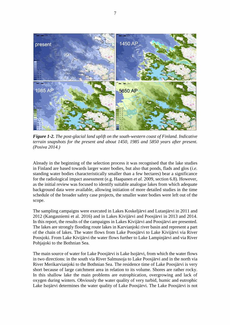
Figure 1-2. The post-glacial land uplift on the south-western coast of Finland. Indicative
terrain snapshots for the present and about 1450, 1985 and 5850 years after present.
(Posiva 2014.)
Already in the beginning of the selection process it was recognised that the lake studies
in Finland are based towards larger water bodies, but also that ponds, flads and glos (i.e.
standing water bodies characteristically smaller than a few hectares) bear a significance
for the radiological impact assessment (e.g. Haapanen et al. 2009, section 6.8). However,
as the initial review was focused to identify suitable analogue lakes from which adequate
background data were available, allowing initiation of more detailed studies in the time
schedule of the broader safety case projects, the smaller water bodies were left out of the
scope.
The sampling campaigns were executed in Lakes Koskeljärvi and Lutanjärvi in 2011 and
2012 (Kangasniemi et al. 2016) and in Lakes Kivijärvi and Poosjärvi in 2013 and 2014.
In this report, the results of the campaigns in Lakes Kivijärvi and Poosjärvi are presented.
The lakes are strongly flooding route lakes in Karvianjoki river basin and represent a part
of the chain of lakes. The water flows from Lake Poosjärvi to Lake Kivijärvi via River
Poosjoki. From Lake Kivijärvi the water flows further to Lake Lampinjärvi and via River
Pohjajoki to the Bothnian Sea.
The main source of water for Lake Poosjärvi is Lake Isojärvi, from which the water flows
in two directions: in the south via River Salmusoja to Lake Poosjärvi and in the north via
River Merikarvianjoki to the Bothnian Sea. The residence time of Lake Poosjärvi is very
short because of large catchment area in relation to its volume. Shores are rather rocky.
In this shallow lake the main problems are eutrophication, overgrowing and lack of
oxygen during winters. Obviously the water quality of very turbid, humic and eutrophic
Lake Isojärvi determines the water quality of Lake Poosjärvi. The Lake Poosjärvi is not

8
regulated and the spring floods are usual and high. In summertime, communities of sedges
dominate large areas of the lake. In the northern part of the Lake Poosjärvi there are dense
horsetail communities. There is an open area in the middle of the lake surrounded by
nympheids and helophytes The birdlife of the lake is rich. Lake Poosjärvi represents
partly a vegetation-overgrown situation, too.
Lake Kivijärvi is rocky, shallow and rich in humus. The inlet, River Poosjoki, comes from
Lake Poosjärvi, so the catchment area of Lake Poosjärvi is also part of the catchment area
of Lake Kivijärvi. In this report the catchment areas are still mainly presented as separate
areas. The outlet from Lake Kivijärvi runs via a fall to the nearby Lake Lampinjärvi. The
Lake Kivijärvi has remained in quite a natural state. European beaver is met in the area.
There is no residential activity ashore of the lake.
The catchment areas of Lakes Kivijärvi and Poosjärvi are mainly forest and mires (Table
1-1, Figure 1-3). There are no fields in the catchment area of Lake Kivijärvi, and fields
cover only 3 % of the catchment area of Lake Poosjärvi. The most common surface soil
type in both catchment areas is medium-grained mineral soil (0.032-0.500 mm) (Figure
1-4; Table 3-2 in Posiva 2014). Other common soil types are peatland and gyttja.
Table 1-1. The charasteristics of Lake Poosjärvi (OL-TMA71) and Lake Kivijärvi (OL-
TMA73) and their catchment areas.
Lake area (km2)
Max depth
(m)
Mean depth
(m)
Shoreline (km)
Catchment area (km2)
Water areas (%)
Fields (%)
Mires (%)
Lake Poosjärvi 3.53 2.50 0.61 36.8 55.6 6.5 3.1 15.6
Lake Kivijärvi 0.56 2.49 0.66 9.4 15.9 4.8 0.0 7.4

9
Figure 1-3. Catchment areas of Lake Poosjärvi (OL-TMA71) and Lake Kivijärvi (OL-
TMA73).
Figure 1-4. Surface soil type (Table 3-2 in Posiva 2012-28) of the catchment areas of
Lake Poosjärvi (OL-TMA71) and Lake Kivijärvi (OL-TMA73), together with modelled
water depth of the lakes.
10
1.2 Data handling and derivation of parameter values
A number of parameters in the models are not directly measurable, and the needed values
require derivation through calculations. Such parameters include concentration ratios
(CR) and distribution coefficients (Kd). In addition, for addressing conceptual and
numerical uncertainties related to the representation of the plant and animal species as
ellipsoids in the dose assessments, the calculated volumes and densities of such ellipsoids
provide useful input to the biosphere assessment. As the topic is common to the entire
report, this section presents how such derived quantities were established in the present
work, after detailing the handling of the raw data.
In the present work, the scope was set so that the calculations are to be done only based
on the arithmetic mean values, if there are several samples contributing to the inventory,
and in general based on best estimates, even though in several cases the available data
would had allowed, with some further effort, estimation of a range of reasonable values.
The calculations were also to be made as a bulk in spreadsheets, and for all the elements
even though the validity of concentration ratios, for example, can be questioned at least
for macronutrients and homeostatically regulated elements. The results were compared to
the previous results from Koskeljärvi and Lutanjärvi (Kangasniemi et al. 2016) and other
results from literature. However, some checking (e.g., the overall range of values and
their maximum/minimum ratio) have been made to detect obvious outliers in the data and
results and to re-iterate with the original field forms or laboratory reports to minimise the
risk of error as far as achievable.
1.2.1 Data handling
Some of the laboratory results could not have been fully quantified due to the
concentration being below the quality-certified limit of quantification (LOQ). However,
in most cases full numerical results from the analytical equipment have been made
available and used here. In addition to values below the LOQ, they also occasionally
contain negative concentration results due to the background corrections and peak
identification in the spectrometer results. In some of the analysis results, the LOQ values
have not been provided separately, but some of the individual results have been delivered
with a < prefix, and it is interpreted that the numerical value would then indicate the LOQ,
below which the actual concentration has been. In order to obtain estimates for the use in
the biosphere assessment for the whole analytical suite of chemical elements, 'fixed
values' accommodating for these lower quality results have been derived with the
principle to overestimate the transfer to the biota and to overestimate the sorption to the
sediment for the needs of cautiousness of the biosphere assessments.

11
1.2.2 Concentration ratios
In the radionuclide transfer models, the transfer from the environmental medium to biota
is represented by the concentration ratio that is the ratio of the concentration in the biota
to that in its living environment, here, water. The concentration ratios in the aquatic
environment are thus defined as (e.g., Hosseini et al. 2008, p. 1408):
CR = Cbiota / Cwater (1)
where CR is the water-to-biota concentration ratio in the units of (µg/kg dry)/(µg/l), Cbiota
is the element concentration (µg/kg dry) in the biota in question, and Cwater is the
respective element concentration in the water representative to the living environment
(µg/l) of the biota. Typically the concentration in the water is determined from filtered
water samples (e.g., Hosseini et al. 2008, p. 1408), preferably so that the filter size is
consistent with the size fraction considered to make the distinction between the dissolved
and particulate species in the water in the model (i.e., linked to the definition of the
suspended solids and the sediment pore water).
Regarding the concentration in the biota, different “compartmentalisations” are needed
by the modelling (e.g., Posiva 2014):
the bulk vegetation for the radionuclide transport modelling;
the edible part of fish and crayfish for the dose assessment for people;
the whole body of biota individuals for the dose assessment for the biota
themselves.
In addition, the same data are needed also to establish quantified conceptual models in
terms of element storages and fluxes in the environment (e.g., Posiva 2014, ch. 4). Even
though the fresh-weight basis is often used for the edible part and the whole body
concentration ratios, the results have been presented here in terms of dry weight
throughout the data, for consistency with Posiva's modelling choices (e.g., Posiva 2014)
and to decrease the notorious variability due to the moisture conditions during field work
and sample processing. The respective dry matter concentrations are tabulated as well in
this report, so the conversion between the dry- and fresh-weight bases should not be
unreasonably tedious – for clarity and the scope of the work, not all possible ways to
normalise and present the data have been utilised here.
From above, it follows that for some concentration ratios single biota samples match
directly with the need (e.g., the samples of the edible portion of the fish), and for some
further calculations are needed to first establish the desired effective concentration (e.g.,
the whole fish or the bulk vegetation). The effective concentration is calculated as the
dry-mass-weighted mean of the relevant samples i:
id
iid
iif
iiif
biotaM
CM
DMm
CDMmC
,
,
,
, (2)
where, mf,i is the fresh biomass in question (kg fresh; e.g., the full mass of the edible or
non-edible fraction of the fish), DMi is the dry mass fraction in sample i (kg dry / kg
fresh), and Ci the element concentration in sample i (µg/kg dry). This is, in other words,
12
the overall inventory in the same biota unit divided by its mass. For the aquatic plants
(macrophytes), the calculation is streamlined as presented to the right in equation (2)
because the area-specific biomass has been readily reported in dry-weight basis; Md,i is
the dry mass per unit area of the part of the vegetation unit (kg/m² in dry; e.g., of the
individual plant species sampled comprising the total living biomass). If several samples
have been aggregated (e.g., by pooling a number of fish individuals in a laboratory
sample), the biomasses mf,i and Md,i refer to the sum of the original samples. The
respective effective dry matter concentrations are calculated in the same way.
It is to be noted that the fraction of ‘all living’ vegetation includes also the mosses (if
present) as so far there has been only a single vegetation compartment in the models (e.g.,
Posiva 2014, section 5.2), but also data regarding only the mosses have been presented as
well due to their somewhat different behaviour in the contaminant transport from that of
vascular plants. Also, clear differentiation of the living and dead parts is often rather
tedious. However, the samples consist mostly of living (green) parts due to the practice
adopted.
1.2.3 Distribution coefficients (Kd)
To determine the solids : solution (i.e., 'pore water') distribution coefficient (partition
coefficient; Kd) of the indigenous elements in the sediments, the sediment samples were
wetted, incubated and centrifuged to separate the fractions before determining the
respective element concentrations. The treatment of the samples and the analytical details
have been presented in section 4.1. From these results of the element concentrations in
the sediment fractions, the distribution coefficients (Kd) were calculated as (Sheppard et
al. 2007, 2009):
Kd = ( Csolids / Cporewater ) (3)
where Kd is the units of (µg/kg dry)/(µg/l), and Csolids is the concentration in the solids
(µg/kg dry), Cporewater the concentration in the extracted pore water (µg/l).
1.3 Related reports
Literature and data sources related to the reference lakes known to the authors are listed
below for further reference, although no specific literature search was made for the
present report.
Water samples, macrophyte survey and sampling, and sediment, fish and macrobenthos
sampling have been reported followingly:
studies at reference lakes and at Olkiluoto conducted in 2010 (Kangasniemi &
Helin 2014)
studies at reference lakes conducted in 2011-2012 (Kangasniemi et al. 2016)
studies at Olkiluoto conducted in 2011-2012 (Kirkkala et al. 2017)
studies at reference rivers conducted in 2014-2015 (Haavisto & Toivola 2017)
13
And additionally:
the most essential biomass and concentration ratio results from the macrophyte
studies at reference lakes Koskeljärvi and Lutanjärvi conducted in 2010
(Kangasniemi et al. 2011)
sediment properties and water depth in the reference lakes (Ojala 2011)
littoral vegetation at lakes Lutanjärvi and Koskeljärvi (Haapanen & Lahdenperä
2011)
Aerial photographs of the reference lakes have been acquired by Posiva in 2010
(Haapanen 2014, p. 59) and at least from Lutanjärvi and Koskeljärvi also in 2013, but not
published as a whole. The present report is a continuation in the series initiated with
Kangasniemi & Helin (2014), whereas the link is less direct with the sediment survey
(Ojala 2011), the littoral survey (Haapanen & Lahdenperä 2011) and the individual
studies listed in below. The latest synthesis of the available site data and literature was
presented in Haapanen et al. (2009), with some additions in Posiva (2013a).
Lakes Poosjärvi and Kivijärvi:
Poosjärvi in general: Hakila & Kalinainen 1992, 2001 (cited in Haapanen et al.
2009, pp. 142‒143, 154‒155);
Kivijärvi macrophytes: Lepistö 2015;
A summary regarding all the three lakes: Haapanen et al. 2009, pp. 154‒155.

14

15
2 SAMPLING LOCATIONS AND RELATED TERMINOLOGY
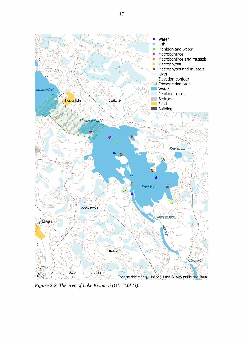
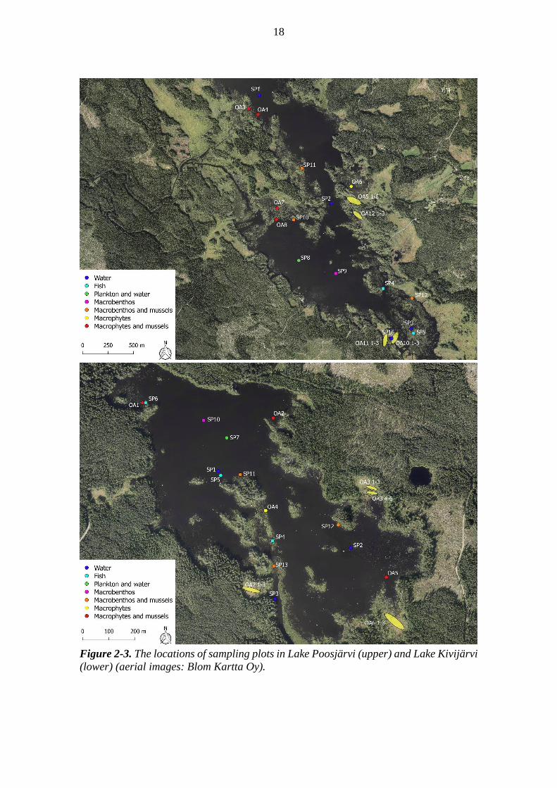
In this chapter the sampling locations are presented with maps in Figures 2-1 to 2-3. The
corresponding detailed coordinates of the sampling locations are presented in Appendix
A. The sampling locations and areas have hierarchical system in their coding. First, the
lake as such is coded in the OL-TMA series with a running identification number. For
Lake Poosjärvi the code is OL-TMA71 and for Lake Kivijärvi it is OL-TMA73.The prefix
“OL” is internal to Posiva’s system and is often not included in the codes in reporting.
Within a lake, sampling areas representing as homogeneous area of vegetation type as
possible (e.g. a reed bed) are identified and coded by suffixing the TMA code with prefix
“OA” and a running number. Within these sampling areas, single sampling points (e.g.
vegetation quadrats) are identified with an additional suffix of “SP” and a running
number. These OA-coded sampling plots, which include several SP-coded plots, are in
the map marked with an ellipse area instead of one point (Figure 2-3). Those ellipses
describe the locations of SP-plots inside the OA-plots. For sample types that are not
readily associated with a certain area, for example water samples, the OA-level is omitted.
It is to be noted that the numbers run separately for the TMA-SP combinatins, for the
TMA-OA combinations and within each TMA-OA combination.

16
Figure 2-1. The area of Lake Poosjärvi (OL-TMA71).
17
Figure 2-2. The area of Lake Kivijärvi (OL-TMA73).
18
Figure 2-3. The locations of sampling plots in Lake Poosjärvi (upper) and Lake Kivijärvi
(lower) (aerial images: Blom Kartta Oy).

19
3 WATER SAMPLES FROM THE LAKES
For this report, the water samples from several locations from Lakes Kivijärvi and
Poosjärvi were collected during the years 2013 and 2014. Samples were collected in
spring, summer, and autumn. The aim of the study was to improve the knowledge of water
quality in these locations and to determine the element concentrations in order to provide
a basis for estimating transfer of different elements to aquatic organisms (macrophytes,
plankton, macrobenthos, fish). Special attention was paid on the key elements. In the
following, results of the water sampling carried out in 2013 and 2014 are reported.
Water quality studies of reference lakes were started in 2010 and 2011 in previous studies
conducted by Posiva (Kangasniemi & Helin 2014, Kangasniemi et al. 2016). In 2010, all
seven reference lakes (Kivijärvi, Poosjärvi, Koskeljärvi, Suomenperänjärvi, Lutanjärvi,
Lampinjärvi, Valkjärvi) and in 2011, five reference lakes (Kivijärvi, Poosjärvi,
Koskeljärvi, Lutanjärvi, Lampinjärvi) were studied. Thus, this report improves the water
quality and element concentration database of the reference lakes.
3.1 Methods
3.1.1 Sampling
In 2013 and 2014, water samples were collected from three sampling points in Lake
Kivijärvi (TMA73-SP1, SP2, SP3) and in Lake Poosjärvi (TMA71-SP1, SP2, SP3).
Water samples were collected simultaneously with the macrophyte sampling campaigns
performed in spring, summer and autumn. Water samples were also taken from a Lake
Poosjärvi sampling point SP16, which is a ditch. Samples were taken as vertical
composite samples covering the water column form the surface down to 20 cm above the
bottom. In spring 2013, Lake Poosjärvi was flooding, and sampling was not possible.
Sampling points and dates are presented in Figure 2-3 and Table 3-1. In addition, water
samples from one sampling point used for plankton studies (Kivijärvi SP7, Poosjärvi SP8)
were collected as composite samples from the euphotic zone. Sampling dates, points, and
depths for plankton sampling points are presented in Table 3-2. Detailed information on
sampling points and depths is presented in Appendix B in Table B-1. All water samples
were collected with the Limnos sampler by Posiva or Water and Environment Research
of South-West Finland Ltd. The water was stored in clean plastic bottles; the water quality
samples were transported in a cooled, insulated bag to the laboratory within the next 24
hours. The samples for the element analyses were stored for several months in a freezer
before sending to the laboratory.
3.1.2 Laboratory analyses
Turbidity, pH, total suspended solids, conductivity, chlorophyll-a, and carbon compounds
(DIC, TIC, TOC, DOC) were analysed in the laboratory of Water and Environment
Research of South-West Finland Ltd with the standard methods. Suspended solids were
determined by filtrating through a 0.4-μm filter ("Nuclepore"). Methods are presented in
Table 3-3.

20
Element concentrations and total nitrogen, total carbon, and phosphorus concentrations
were analysed by ALS Scandinavia AB (Sweden). Analysis of elements was carried out
as a quantitative screening-analysis with ICP-SFMS. Cl, Br, and I were analysed after
separate analytical run. The samples were filtrated on 0.45 µm before acidification and
analysis. Methods are presented in Table 3-3.
Table 3-1. Sampling points and dates (day.month.year) of water samples for water quality
and element concentration analyses in Lakes Kivijärvi and Poosjärvi in 2013–2014.
Kivijärvi
SP1
Kivijärvi
SP2
Kivijärvi
SP3
Poosjärvi
SP1
Poosjärvi
SP2
Poosjärvi SP3
Poosjärvi SP16
Sampling date
Sampling date
Sampling date
Sampling date
Sampling date
Sampling date
Sampling date
6.5.2013 26.8.2013
14.10.2103 13.5.2014 18.8.204
20.10.2014
6.5.2013 26.8.2013
14.10.2103 13.5.2014 18.8.2014
20.10.2014
6.5.2013 26.8.2013
14.10.2103 13.5.2014 18.8.2014
20.10.2014
- 26.8.2013
14.10.2103 13.5.2014 18.8.2014
20.10.2014
- 26.8.2013 14.10.2103 13.5.2014 18.8.2014 20.10.2014
- 26.8.2013
14.10.2103 13.5.2014 18.8.2014
20.10.2014
- 26.8.2013
14.10.2013 13.5.2014 18.8.2014
20.10.2014
Table 3-2. Sampling points, dates and depths (m) of water samples of Lakes Kivijärvi
and Poosjärvi in 2013 and 2014. Same points were used for plankton studies.
Kivijärvi SP7 Poosjärvi SP8
Time of year Sampling date Sampling depth m Sampling date Sampling depth m
Autumn 2013 Spring 2014
Summer 2014 Autumn 2014
18.9.2013 21.5.2014 13.8.2014 7.10.2014
0–2.0 0–2.0 0–2.0 0–2.0
19.9.2013 21.5.2014 14.8.2014 7.10.2014
0–1.3 0–1.0 0–1.0 0–1.3
Table 3-3. Methods for water quality determination used in analyses conducted by Water
and Environment Research of South-West Finland Ltd and ALS Scandinavia AB.
Variable Method/Standard
Water and Environment Research of South-West Finland Ltd.
Turbidity (nephelometric) SFS-EN ISO 7027:2000
pH (25 °C) SFS 3021:1974 (TL27)
Total suspended solids (0.4 µm membrane filter) The laboratory’s in-house method
Conductivity (at 25 °C) SFS-EN 27888:1994
Chlorophyll-a SFS 5772:1993
Dissolved inorganic carbon (DIC) SFS-EN 1484:1997
Total inorganic carbon (TIC) SFS-EN 1484:1997
Total organic carbon (TOC) SFS-EN 1484:1997
Dissolved organic carbon (DOC) SFS-EN 1484:1997
ALS Scandinavia AB
Element concentrations ICP-SFMS
Total nitrogen (N-tot) DIN EN ISO 11905-1 (H36)
Total carbon (C-tot) DIN EN 1484-H3
Phosphorus (P) DIN EN ISO 11885-E22
21
3.2 Results
3.2.1 Water quality
The summary of the water quality parameters in Lakes Kivijärvi and Poosjärvi in 2013
and 2014 is presented in Tables 3-4A and 3-4B. In Table 3-4A, arithmetic means of all
sampling points and times are presented separately for both lakes and years. In addition,
also the arithmetic means of both lakes and years were calculated and presented in Table
3-4A. In Table 3-4B, arithmetic means of all sampling points and both years are presented
separately for both lakes and three seasons (spring, summer, autumn). The full data set
for each sampling date and point is presented in Appendix B (Table B-2). The water
temperature data and Secchi depths are presented in Appendix B (Table B-1).
3.2.2 Element concentrations
The summary of the key element concentrations in water samples from the Lakes
Kivijärvi and Poosjärvi in 2013 and 2014 is presented in Tables 3-5A and 3-5B. The
statistics have been calculated similarly as for basic water quality results. Unreliable
laboratory results such as negative values, values below the LOQ (limits of
quantification), and values over the LOQ but marked with “<” were not used in
calculations. The full data set for each sampling date and point and for all elements as
well as limits of quantification (LOQ) is presented in Appendix B (Tables B-3 and B-4).
3.3 Discussion
3.3.1 Water quality
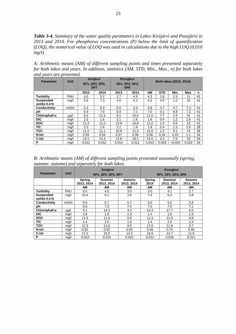
There were no major differences in basic water quality parameters between the lakes
(Tables 3-4A, 3-4B). However, some differences between the study years were observed
probably due to the weather conditions. In addition, there were some seasonal differences.
In both lakes, turbidity and concentrations of suspended solids were higher in spring
compared to summer and autumn. Further, concentrations of chlorophyll-a were at their
highest in summer in both lakes. During autumn, the carbon and phosphorus
concentrations were lower compared to spring and summer.
The phosphorus concentrations in both lakes and years were mainly typical for slightly
eutrophic lakes, and the differences between the lakes and years were minor. The
chlorophyll-a concentrations were clearly higher in 2014 compared to 2013 mainly due
to the high values of chlorophyll-a in August 2014 in both lakes (Appendix B, Table B-
2). In addition, the mean turbidity and the concentrations of suspended solids and total C
were slightly higher in 2014 in both lakes compared to year 2013. In both years, pH values
were near neutral and conductivity was low.
Compared to the previous studies in 2010 and 2011, the chlorophyll-a levels were higher
as a mean of both lakes in years 2013–2014 (Kangasniemi et al. 2016, Table 3-2). In
addition, in 2013–2014, pH values were slightly higher than in 2010–2011. The
concentration of suspended solids appeared to be higher in 2013–2014 compared to 2010–
2011 possibly due to the differences in chlorophyll-a and thus in phytoplankton biomass.

22
3.3.2 Element concentrations
There were no clear differences in element concentrations between the two lakes, but
some differences between the years were found (Table 3-5a). The mean concentrations
of chlorine (Cl) and strontium (Sr) out of the key elements tended to be higher in 2014
compared to 2013 in both lakes. For other elements, there were also some similar trends
observed in the concentrations between the study years 2013 and 2014 (Appendix B,
Tables B-3 and B-4). In both lakes, the concentrations of Br, Ca, K, Mg, S, and Si were
higher in 2014 compared to 2013. On the contrary, the concentrations of Pb, Al and Fe
were higher in 2013 compared to 2014. The variation between the minimum and
maximum concentrations of the key elements was mainly fivefold to twentyfold.
The concentrations of the key elements did not vary significantly between the three
seasons in either of the lakes (Table 3-5A).
In previous studies on reference lakes, there were differences in analysing element
concentrations concerning filtering of the samples. However, the comparisons between
different filter sizes (0.2 and 0.45 µm) and no-filtering shows that there are no major
differences between the different methods used (Appendix A in Kirkkala et al. 2017). In
this study, only filtering with 0.45 µm filter was used.
23
Table 3-4. Summary of the water quality parameters in Lakes Kivijärvi and Poosjärvi in
2013 and 2014. For phosphorus concentrations (P) below the limit of quantification
(LOQ), the numerical value of LOQ was used in calculations due to the high LOQ (0,010
mg/l).
A: Arithmetic means (AM) of different sampling points and times presented separately
for both lakes and years. In addition, statistics (AM, STD, Min., Max., n) for both lakes
and years are presented.
Parameter Unit Kivijärvi
SP1, SP2, SP3, SP7
Poosjärvi
SP1, SP2, SP3, SP8
Both lakes (2013, 2014)
2013 2014 2013 2014 AM STD Min. Max. n
Turbidity FNU 4.0 5.2 2.7 4.5 4.3 1.8 2.5 11 41
Suspended solids 0.4 N
mg/l 5.9 7.3 4.6 6.2 6.2 4.0 1.2 26 41
Conductivity mS/m 5.3 6.3 5.0 6.3 5.8 0.7 4.7 7.3 41
pH 6.9 7.0 6.9 7.1 7.0 0.1 6.8 7.2 41
Chlorophyll-a µg/l 6.0 12.3 8.1 15.6 11.0 7.7 2.5 31 41
DIC mg/l 2.3 1.6 2.1 1.6 1.8 0.4 1.2 2.6 41
DOC mg/l 11.3 11.0 10.9 10.8 11.0 1.0 9.5 13 41
TIC mg/l 2.3 1.6 2.2 1.6 1.8 0.4 1.3 2.6 38
TOC mg/l 11.0 11.1 10.8 11.2 11.0 1.2 9.1 13 38
N-tot mg/l 0.59 0.54 0.57 0.56 0.56 0.18 0.22 1.1 34
C-tot mg/l 14.1 15.4 12.8 16.1 14.5 2.2 7.5 19 34
P mg/l 0.012 0.012 0.014 0.011 0.013 0.003 <0.010 0.022 34
B: Arithmetic means (AM) of different sampling points presented seasonally (spring,
summer, autumn) and separately for both lakes.
Parameter Unit Kivijärvi
SP1, SP2, SP3, SP7
Poosjärvi
SP1, SP2, SP3, SP8
Spring 2013, 2014
Summer 2013, 2014
Autumn 2013, 2014
Spring 2014
Summer 2013, 2014
Autumn 2013, 2014
AM AM AM AM AM AM
Turbidity FNU 6.5 4.5 3.0 5.0 4.1 2.7
Suspended solids 0.4 N
mg/l 10.4 6.1 3.6 7.4 6.3 3.8
Conductivity mS/m 6.0 5.7 5.7 6.5 5.5 5.8
pH 6.9 7.0 7.0 7.0 7.0 7.1
Chlorophyll-a µg/l 9.1 14.2 4.2 14.3 17.7 6.6
DIC mg/l 1.8 1.9 1.9 1.4 1.8 1.9
DOC mg/l 11.9 11.6 9.8 11.3 11.5 9.8
TIC mg/l 1.4 2.0 1.9 1.4 2.0 1.9
TOC mg/l 12.3 11.8 9.5 12.0 11.8 9.7
N-tot mg/l 0.52 0.62 0.53 0.49 0.75 0.40
C-tot mg/l 17.0 15.0 13.3 16.8 14.7 11.9
P mg/l 0.013 0.013 0.010 0.012 0.016 0.011

24
Table 3-5. Summary of the element concentrations (μg/l) of the key elements in Lakes
Kivijärvi and Poosjärvi in 2013 and 2014.
A: Arithmetic means of different sampling points and times presented separately for both
lakes and years. In addition, statistics (AM, STD, Min., Max., n) for both lakes and years
are presented. N.A. = analysis not available.
Kivijärvi SP1, SP2, SP3, SP7
Poosjärvi SP1, SP2, SP3, SP8,
SP16 Both lakes
year 2013 2014 2013 2014 2013 and 2014
Element AM AM AM AM AM STD Min. Max. n
Ag 0.013 0.05 0.012 0.012 0.028 0.033 0.01 0.107 12
Cl 2770 3240 2100 3030 2880 921 244 4330 43
Cs 0.009 0.009 0.008 0.009 0.009 0.002 0.003 0.013 43
I 3.53 6.83 3.37 3.86 4.53 5.07 1.55 36.4 43
Mo 0.111 0.131 0.109 0.123 0.12 0.045 0.024 0.25 43
Nb 0.006 0.003 0.003 0.003 0.004 0.003 0.001 0.014 43
Ni 1.54 1.5 1.37 1.54 1.5 0.286 0.691 1.95 43
Pb 0.059 0.021 0.054 0.018 0.035 0.023 0.008 0.079 40
Pd N.A. 0.001 N.A. 0.002 0.002 0.001 0.001 0.005 7
Se 0.461 0.088 0.169 0.145 0.182 0.175 0.051 0.591 16
Sn 0.028 0.016 0.007 0.008 0.016 0.013 0.007 0.042 11
Sr 21.8 26 18.7 28.9 24.8 5.51 9 42.6 43
B: Arithmetic means (AM) of different sampling points presented seasonally (spring,
summer, autumn) and separately for both lakes. N.A. = analysis not available.
Kivijärvi SP1, SP2, SP3, SP7
Poosjärvi SP1, SP2, SP3, SP8, SP16
season Spring 2013, 2014
Summer 2013, 2014
Autumn 2013, 2014
Spring 2014
Summer 2013, 2014
Autumn 2013, 2014
Element AM AM AM AM AM AM
Ag 0.054 0.023 0.013 0.012 0.012 N.A.
Cl 2630 3260 3160 2590 2830 2670
Cs 0.009 0.011 0.008 0.008 0.011 0.008
I 8.0 4.8 3.3 3.5 4.3 3.1
Mo 0.104 0.159 0.096 0.101 0.147 0.095
Nb 0.008 0.003 0.003 0.004 0.003 0.003
Ni 1.7 1.6 1.3 1.8 1.6 1.2
Pb 0.036 0.033 0.047 0.015 0.029 0.043
Pd 0.001 N.A. N.A. 0.002 0.005 N.A.
Se 0.246 0.127 0.134 0.067 0.193 0.135
Sn 0.020 0.031 N.A. 0.008 0.007 N.A.
Sr 24.2 25.1 22.9 24.8 27.6 23.6

25
4 SURFACE SEDIMENTS
In this chapter, the sampling methods and the results of element concentrations and
distribution coefficients (Kd) of sediment samples from Lakes Kivijärvi and Poosjärvi in
2013 and 2014 are presented.
4.1 Methods
Surface sediment samples were collected from Lakes Poosjärvi and Kivijärvi during the
macrophyte sampling campaigns (Table 4-1). The samples were analysed for sediment
properties and element concentrations. The sampling locations are illustrated in Figure 2-
3. The coordinates are listed in Appendix A.
Table 4-1. General information of the sediment samples collected from Lake Poosjärvi
and Lake Kivijärvi in May (M), August (A) and October (O) 2013 and 2014, according
to Posiva’s biosphere assessment biotopes (table 3-1 in Posiva 2014). Sampling area
Assessment biotope
Dominating species
Sampling 2013
Sampling 2014
Surface sediment type
Lake Poosjärvi
OA3 photic soft bottom
horsetail - A gyttja (org.)
OA5 reed bed mixed O O root layer, gyttja/clay
OA6 photic soft bottom
floating pondweed O MAO gyttja (org.)/clay
OA7 photic soft bottom
horsetail - MAO gyttja (org.)/clay
OA8 photic soft bottom
yellow water-lily AO MAO gyttja (org.)/clay
OA10 reed bed bulrush - MO gyttja/clay
OA11 reed bed sedge O AO root layer, gyttja/clay
OA12 photic soft bottom
marsh cinquefoil O MAO root layer,
gyttja/clay/sand/gravel
Lake Kivijärvi
OA1 photic soft bottom
yellow water-lily MAO - gyttja (org.)/clay/sand
OA2 photic soft bottom
yellow water-lily MAO MAO gyttja (org.)/clay
OA3 reed bed common reed - A gravel
OA5 photic soft bottom
yellow water-lily A - gyttja (org.)/clay
OA7 reed bed sedge - A gyttja (org.)
In Poosjärvi in sampling plot OA5 and in Kivijärvi in sampling plot OA3 three sub-
samples (1-3) were combined as one sample representing dryer part of the sampling plot
closer to the shore, and other three combined subsamples (3-6) represent an area a several
meters outwards from the shoreline, which represent the more wetter part of the sampling
plot. In other sampling plots three sub-samples were taken from each plot and they were
combined as one sample.
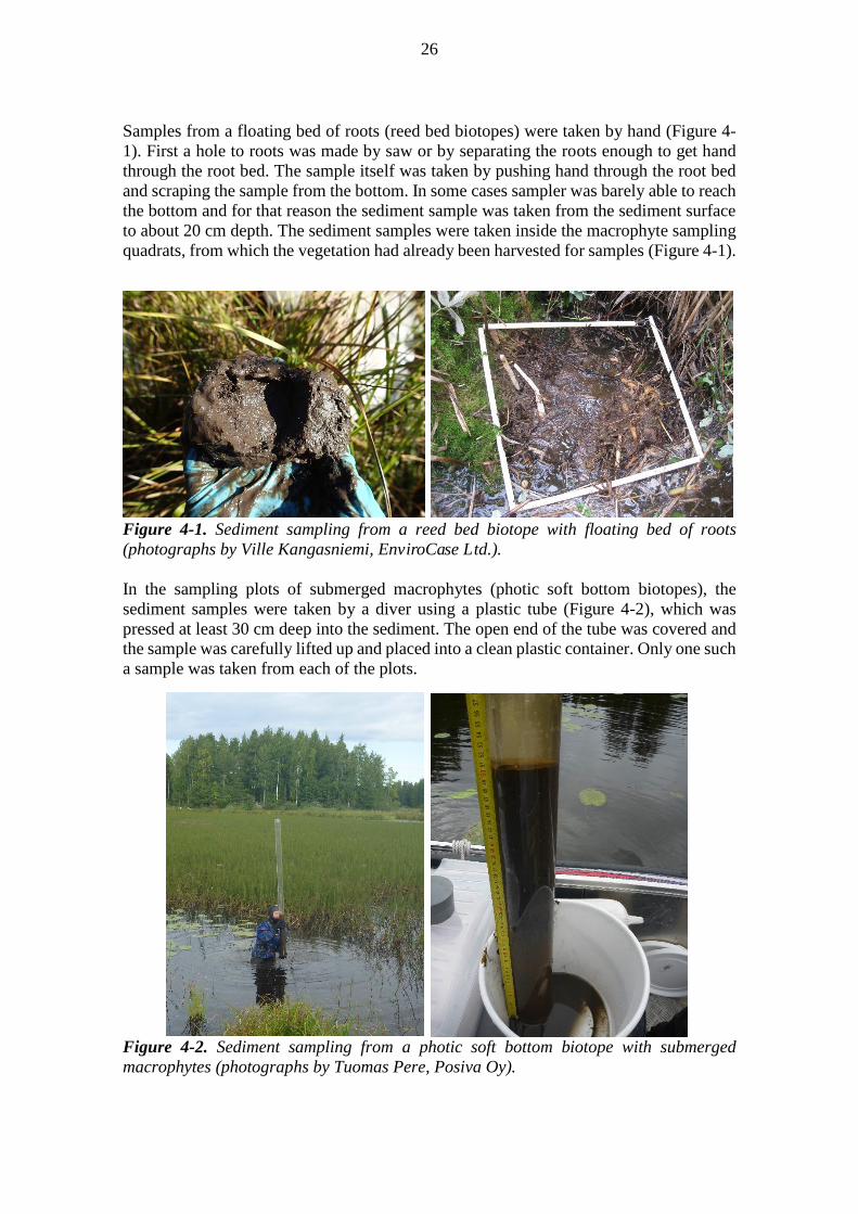
26
Samples from a floating bed of roots (reed bed biotopes) were taken by hand (Figure 4-
1). First a hole to roots was made by saw or by separating the roots enough to get hand
through the root bed. The sample itself was taken by pushing hand through the root bed
and scraping the sample from the bottom. In some cases sampler was barely able to reach
the bottom and for that reason the sediment sample was taken from the sediment surface
to about 20 cm depth. The sediment samples were taken inside the macrophyte sampling
quadrats, from which the vegetation had already been harvested for samples (Figure 4-1).
Figure 4-1. Sediment sampling from a reed bed biotope with floating bed of roots
(photographs by Ville Kangasniemi, EnviroCase Ltd.).
In the sampling plots of submerged macrophytes (photic soft bottom biotopes), the
sediment samples were taken by a diver using a plastic tube (Figure 4-2), which was
pressed at least 30 cm deep into the sediment. The open end of the tube was covered and
the sample was carefully lifted up and placed into a clean plastic container. Only one such
a sample was taken from each of the plots.
Figure 4-2. Sediment sampling from a photic soft bottom biotope with submerged
macrophytes (photographs by Tuomas Pere, Posiva Oy).

27
4.1.1 Sample analysis
The sediment samples were analysed by Laboratory of Radiochemistry, University of
Helsinki (HYRL) (Lusa 2017). Samples were not sieved before sending to analyzing
laboratory. Coarser roots and larger stones have been excluded from the sample before
analyzing.
Element concentrations were analysed in 2013---2014 from the both the pore water and
the solid fraction of the sediment samples to allow calculation of the distribution
coefficients (Kd; see section 1.3.3) for the indigenous elements in the sediment samples.
For the solid fractions, different digestion methods were applied to distinguish the
“pseudo-total’’ and the ‘‘bioavailable’’ concentrations. The details of these analyses are
explained in the paragraphs nearest below.
To analyse the pore water from the sediment, the incubated samples were directly
centrifuged at 5000 rpm for 15 min after one week at room temperature. Following
centrifugation, the extracted pore water was collected in a syringe, and aspirated hrough
a 0.45 µm filter. One aliquot was acidified using suprapure HNO3 before the
determination of 61 elements by ICP-MS, and a second was taken directly for the
quantification of I by ICP-MS in separate alkaline analytical run (in NH3). HCl + NO3
addition was used for Ge, Lu, Rd, Sb, Sn, W and Zr. F, Br and Cl were measured
separately using IC and for them numerical LOQs could not have been determined.
After the pore water extraction explained above, the remaining incubated solid fraction
of the sample was first dried at 50°C prior to further analysis. Separate measurements of
the dry matter content at 105°C were carried out based on standard SS 02 81 13-1 in order
to express the element concentrations determined from the material dried at 50°C in terms
of the dry mass normalised to 105°C.
After drying of the solid fraction of the samples the bioavailable element concentrations
were determined. On the average 2.76 g of the incubated, dried and homogenised mineral
soil/sediment samples were weighed. In the analyses, the ratio of mineral soil/sediment
samples to NH4Ac solution was 1:10. The samples were leached in NH4Ac (NH4Ac-
CH3COOH) solution buffered at pH 4.5 for 16 hours in overhead shaker. After dilution,
the leachates were analyzed for 61 elements by ICP-MS with HNO3 addition. HCl-HNO3
addition was used for Ge, Lu, Rb, Sb, Sn, W and Zr. Separate analysis (alkaline in NH3)
for I was driven with ICP-MS. Concentration of Cl, F, Br and S cannot be analyzed using
IC (as was done for pore water samples) in HNO3 or NH4Ac containing solutions.

28
4.2 Results
The general information of the sediment samples are summarised in Table 4-1. The
element concentrations in soil solution (pore water) and in the solids (bioavailable and
pseudo-total) and corresponding Kd values in Lake Poosjärvi and Lake Kivijärvi are
presented in tables 4-2 to 4-9. The detailed element concentration data is presented in
Appendix C.
As a summary, the sequence of the tables is:
Table 4-2: Element concentrations in the soil solution and in the solids from Lake
Poosjärvi in 2013
Table 4-3:The corresponding Kd values from Lake Poosjärvi in 2013
Table 4-4: Element concentrations in the soil solution and in the solids from Lake
Poosjärvi in 2014
Table 4-5: The corresponding Kd values from Lake Poosjärvi in 2014
Table 4-6: Element concentrations in the soil solution and in the solids from Lake
Kivijärvi in 2013
Table 4-7: The corresponding Kd values from Lake Kivijärvi in 2013
Table 4:8: Element concentrations in the soil solution and in the solids from Lake
Kivijärvi in 2014
Table 4-9: The corresponding Kd values from Lake Kivijärvi in 2014

29
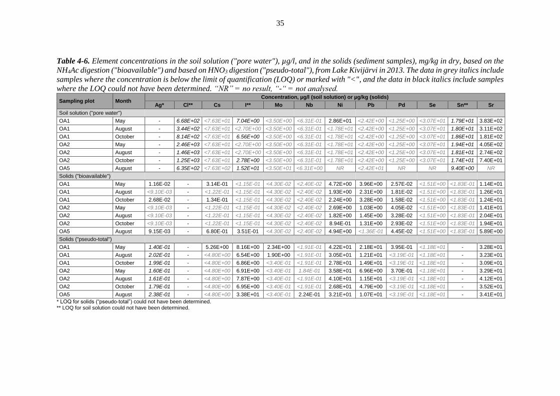
Table 4-2. Element concentrations in the soil solution ("pore water"), µg/l, and in the solids (sediment samples), mg/kg in dry, based on the
NH4Ac digestion ("bioavailable") and based on HNO3 digestion ("pseudo-total"), from Lake Poosjärvi in 2013. The data in grey italics
include samples where the concentration is below the limit of quantification (LOQ) or marked with "<", and the data in black italics include
samples where the LOQ could not have been determined. “NR” = no result, “-“ = not analysed.
Sampling plot Month Concentration, µg/l (soil solution) or µg/kg (solids)
Ag* Cl** Cs I** Mo Nb Ni Pb Pd Se Sn** Sr
Soil solution ("pore water")
OA5 Drier half October - 5.77E+03 <7.63E+01 4.35E+00 <3.50E+00 <6.31E-01 <1.78E+01 4.73E+00 <1.25E+00 <3.07E+01 1.15E+01 3.60E+01
OA5 Submerged half October - 1.91E+03 <7.63E+01 <2.70E+00 <3.50E+00 <6.31E-01 <1.78E+01 <2.42E+00 <1.25E+00 <3.07E+01 1.70E+01 2.02E+02
OA6 October - 1.90E+03 <7.63E+01 4.12E+01 <3.50E+00 <6.31E-01 <1.78E+01 <2.42E+00 <1.25E+00 <3.07E+01 1.43E+01 6.39E+01
OA8 August - 4.41E+03 <7.63E+01 4.01E+01 <3.50E+00 <6.31E-01 NR 9.33E+00 NR NR 1.74E+01 NR
OA8 October - 5.26E+03 <7.63E+01 5.15E+01 <3.50E+00 <6.31E-01 3.47E+01 <2.42E+00 <1.25E+00 <3.07E+01 1.83E+01 1.73E+03
OA11 October - 1.73E+03 <7.63E+01 3.61E+00 <3.50E+00 <6.31E-01 <1.78E+01 <2.42E+00 <1.25E+00 <3.07E+01 1.98E+01 5.72E+01
OA12 October - 2.50E+03 <4.48E+00 <2.70E+00 1.73E+00 <8.88E-01 <9.28E+00 <4.96E+00 <3.38E-01 <5.54E+01 2.17E+01 3.37E+02
Solids ("bioavailable")
OA5 Drier half October <9.10E-03 - <1.22E-01 <1.15E-01 <4.30E-02 <2.40E-02 2.46E+00 1.52E+01 2.22E-02 <1.51E+00 <1.83E-01 1.01E+01
OA5 Submerged half October 1.12E-02 - 1.24E-01 <1.15E-01 <4.30E-02 <2.40E-02 2.27E+00 7.46E+00 2.11E-02 <1.51E+00 <1.83E-01 8.14E+00
OA6 October <9.10E-03 - 5.57E-01 <1.15E+02 <4.30E-02 <2.40E-02 1.01E+01 6.12E+00 4.70E-02 <1.51E+00 <1.83E-01 2.34E+01
OA8 August 1.09E-02 - <1.22E-01 9.12E-01 <4.30E-02 <2.40E-02 1.14E+01 1.68E-01 7.81E-02 <1.51E+00 <1.83E-01 1.80E+01
OA8 October <9.10E-03 - 1.62E-01 3.70E-01 <4.30E-02 <2.40E-02 6.06E+00 1.94E+00 4.73E-02 <1.51E+00 <1.83E-01 2.11E+01
OA11 October <9.10E-03 - 1.35E-01 <1.15E-01 <4.30E-02 3.08E-02 3.42E+00 5.56E+00 5.73E-02 <1.51E+00 <1.83E-01 5.12E+00
OA12 October <9.10E-03 - <1.22E-01 <1.15E-01 <4.30E-02 <2.40E-02 1.39E+00 5.68E+00 2.28E-02 <1.51E+00 <1.83E-01 1.15E+01
Solids ("pseudo-total")
OA5 Drier half October 1.63E-01 - <4.80E+00 4.97E+00 2.47E+00 <1.91E-01 2.98E+01 3.96E+01 3.77E-01 <1.18E+01 - 1.94E+01
OA5 Submerged half October 1.42E-01 - <4.80E+00 6.20E+00 <3.40E-01 <1.91E-01 2.74E+01 2.33E+01 <3.19E-01 <1.18E+01 - 1.78E+01
OA6 October 2.50E-01 - <4.80E+00 1.22E+01 7.66E+00 3.46E-01 5.18E+01 2.32E+01 2.32E+00 <1.18E+01 - 4.49E+01
OA8 August 2.32E-01 - 6.34E+00 3.40E+01 1.56E+00 2.83E-01 4.31E+01 1.03E+01 <3.19E-01 <1.18E+01 - 4.77E+01
OA8 October 1.71E-01 - <4.80E+00 3.71E+01 1.59E+00 5.08E-01 4.00E+01 9.82E+00 <3.19E-01 <1.18E+01 - 4.59E+01
OA11 October 2.22E-01 - <4.80E+00 1.02E+01 3.62E+00 <1.91E-01 3.59E+01 1.65E+01 5.61E-01 <1.18E+01 - 1.79E+01
OA12 October 1.84E-01 - <4.80E+00 1.27E+01 1.23E+01 <1.91E-01 2.22E+01 2.29E+01 1.40E+00 <1.18E+01 - 2.22E+01
* LOQ for solids (“pseudo-total”) could not have been determined. ** LOQ for soil solution could not have been determined.

30
Table 4-3. The corresponding Kd values (mg/kg 105°-dry)/(µg/l) based on the NH4Ac digestion ("bioavailable") and based on HNO3 digestion
("pseudo-total"), from Lake Poosjärvi in 2013. The data in grey italics include samples where the concentration was below the limit of
quantification (LOQ) or marked with "<"; for these, the numerical value of LOQ/2 for soil solution and LOQ for solids are used as a
surrogate. The data in black italics include samples where the LOQ for soil solution could not have been determined. Kd values couldn’t be
calculated for elements Ag and Cl and for some single samples, due to missing concentration results.
Sampling plot Month Calculated Kd values (µg/kg 105°C-dry)/(µg/l)
Cs I* Mo Nb Ni Pb Pd Se Sn* Sr
Solids ("bioavailable")
OA5 Drier half October 3.20 26.4 24.6 80.0 276 3 210 34.2 98.4 15.9 280
OA5 Submerged half October 3.24 85.2 24.6 80.0 255 6 220 32.4 98.4 10.8 40.4
OA6 October 14.6 2.79 24.6 80.0 1 130 5 100 72.3 98.4 12.8 367
OA8 August 3.20 22.7 24.6 80.0 - 18.0 - - 10.5 -
OA8 October 4.24 7.19 24.6 80.0 175 1 620 72.8 98.4 10.0 12.2
OA11 October 3.54 31.9 24.6 103 385 4 630 88.1 98.4 9.27 89.4
OA12 October 54.2 85.2 24.8 53.3 299 2 270 152 54.5 8.43 34.2
Solids ("pseudo-total")
OA5 Drier half October 126 1 140 1 410 637 3 350 8 370 581 769 62 538
OA5 Submerged half October 126 4 590 194 637 3 080 19 400 491 769 42 88.4
OA6 October 126 297 4 380 1 150 5 820 19 300 3 560 769 50 703
OA8 August 166 848 889 942 - 1 100 - - 41 -
OA8 October 126 720 909 1 700 1 150 8 180 491 769 39 26.6
OA11 October 126 2 830 2 070 637 4 030 13 800 863 769 36 313
OA12 October 2 130 9 420 7 080 424 4 770 9 180 9 350 426 33 65.8
* LOQ for soil solution could not have been determined

31
Table 4-4. Element concentrations in the soil solution ("pore water"), µg/l, and in the solids (sediment samples), mg/kg in dry, based on the
NH4Ac digestion ("bioavailable") and based on HNO3 digestion ("pseudo-total"), from Lake Poosjärvi in 2014. The data in grey italics
include samples where the concentration is below the limit of quantification (LOQ) or marked with "<", and the data in black italics include
samples where the LOQ could not have been determined. “NR” = no result, “-“ = not analysed.
* LOQ for solids (“pseudo-total”) could not have been determined. ** LOQ for soil solution could not have been determined.
Sampling plot Month Concentration, µg/l (soil solution) or µg/kg (solids)
Ag* Cl** Cs I** Mo Nb Ni Pb Pd Se Sn** Sr
Soil solution ("pore water")
OA3 August - 1.10E+03 <7.63E+01 1.42E+01 <3.50E+00 <6.31E-01 2.33E+01 <2.42E+00 <1.25E+00 <3.07E+01 1.70E+01 3.16E+02
OA5 Drier half October - 6.25E+03 <7.63E+01 3.78E+00 <3.50E+00 <6.31E-01 <1.78E+01 <2.42E+00 <1.25E+00 <3.07E+01 1.45E+01 6.67E+01
OA5 Submerged half October - 2.48E+03 <7.63E+01 <2.70E+00 <3.50E+00 <6.31E-01 <1.78E+01 <2.42E+00 <1.25E+00 <3.07E+01 1.54E+01 1.04E+02
OA6 May - 2.65E+03 <7.63E+01 7.75E+00 <3.50E+00 <6.31E-01 1.32E+02 <2.42E+00 <1.25E+00 <3.07E+01 1.82E+01 8.45E+02
OA6 August - 1.01E+03 <7.63E+01 2.85E+00 <3.50E+00 <6.31E-01 1.49E+02 <2.42E+00 <1.25E+00 <3.07E+01 1.76E+01 8.59E+02
OA6 October - 2.94E+03 <7.63E+01 9.62E+00 <3.50E+00 <6.31E-01 1.37E+02 <2.42E+00 <1.25E+00 <3.07E+01 1.74E+01 8.63E+02
OA7 May - 1.88E+03 1.15E+01 7.73E+00 7.80E+00 <8.88E-01 <9.28E+00 <4.96E+00 <3.38E-01 <5.54E+01 2.35E+01 1.00E+02
OA7 August - 3.42E+03 <4.48E+00 1.91E+01 2.80E+00 <8.88E-01 8.45E+01 <4.96E+00 <3.38E-01 <5.54E+01 2.04E+01 4.28E+02
OA7 October - 8.01E+02 <7.63E+01 8.50E+00 <3.50E+00 <6.31E-01 <1.78E+01 <2.42E+00 <1.25E+00 <3.07E+01 1.79E+01 1.27E+02
OA8 May - 8.63E+03 <7.63E+01 7.18E+01 <3.50E+00 <6.31E-01 <1.78E+01 <2.42E+00 <1.25E+00 <3.07E+01 1.73E+01 1.66E+03
OA8 August - 1.07E+04 <7.63E+02 1.28E+01 <3.50E+01 <6.31E+00 5.22E+02 <2.42E+01 <1.25E+01 <3.07E+02 1.16E+01 2.35E+03
OA8 October - 2.73E+03 <7.63E+01 6.25E+00 <3.50E+00 <6.31E-01 3.26E+01 <2.42E+00 <1.25E+00 <3.07E+01 1.78E+01 1.08E+03
OA10 May - 1.41E+03 <7.63E+01 8.04E+00 1.26E+01 <6.31E-01 4.52E+01 9.30E+00 1.78E+00 <3.07E+01 2.23E+01 1.47E+03
OA10 October - 2.52E+03 <7.63E+01 3.51E+00 8.01E+00 <6.31E-01 <1.78E+01 3.32E+00 <1.25E+00 <3.07E+01 2.00E+01 3.53E+02
OA11 August - 1.99E+03 <7.63E+01 5.27E+00 <3.50E+00 <6.31E-01 <1.78E+01 <2.42E+00 <1.25E+00 <3.07E+01 1.75E+01 6.55E+01
OA11 October - 1.96E+03 <7.63E+01 3.61E+00 <3.50E+00 <6.31E-01 2.21E+01 <2.42E+00 <1.25E+00 <3.07E+01 1.68E+01 7.56E+01
OA12 May - 3.18E+03 <7.63E+01 3.70E+00 <3.50E+00 <6.31E-01 <1.78E+01 <2.42E+00 <1.25E+00 <3.07E+01 1.77E+01 1.51E+02
OA12 August - 4.41E+03 <7.63E+01 <2.70E+00 1.84E+01 1.19E+00 <1.78E+01 1.52E+01 <1.25E+00 <3.07E+01 2.10E+01 6.50E+01
OA12 October - 2.02E+03 <7.63E+01 7.11E+00 <3.50E+00 <6.31E-01 3.34E+01 <2.42E+00 <1.25E+00 <3.07E+01 1.80E+01 3.38E+02
Solids ("bioavailable")
OA3 August <9.10E-03 - 1.33E-01 <1.15E-01 <4.30E-02 <2.40E-02 7.29E+00 5.57E+00 2.99E-02 <1.51E+00 <1.83E-01 1.05E+01
OA5 Drier half October 9.99E-03 - <1.22E-01 <1.15E-01 <4.30E-02 <2.40E-02 2.62E+00 8.14E+00 1.66E-02 <1.51E+00 <1.83E-01 1.06E+01
OA5 Submerged half October <9.10E-03 - 1.45E-01 <1.15E-01 <4.30E-02 <2.40E-02 2.53E+00 5.52E+00 2.69E-02 <1.51E+00 <1.83E-01 7.70E+00
OA6 May <9.10E-03 - 1.85E-01 <1.15E-01 <4.30E-02 <2.40E-02 5.11E+00 1.44E+00 4.38E-02 <1.51E+00 <1.83E-01 1.47E+01
OA6 August <9.10E-03 - <1.22E-01 <1.15E-01 <4.30E-02 <2.40E-02 6.30E+00 5.94E+00 3.88E-02 <1.51E+00 <1.83E-01 1.44E+01
OA6 October 1.05E-02 - <1.22E-01 <1.15E-01 <4.30E-02 <2.40E-02 4.78E+00 2.54E+00 3.79E-02 <1.51E+00 <1.83E-01 1.34E+01
OA7 May <9.10E-03 - <1.22E-01 <1.15E-01 <4.30E-02 <2.40E-02 3.98E+00 3.47E+00 2.91E-02 <1.51E+00 <1.83E-01 1.84E+01
OA7 August 1.38E-02 - <1.22E-01 <1.15E-01 <4.30E-02 <2.40E-02 4.97E+00 3.05E+00 2.59E-02 <1.51E+00 <1.83E-01 1.18E+01
OA7 October <9.10E-03 - <1.22E-01 <1.15E-01 <4.30E-02 <2.40E-02 3.62E+00 5.97E+00 3.22E-02 <1.51E+00 <1.83E-01 1.64E+01

32
Table 4-4 (cont’d).
Sampling plot Month Concentration, µg/l (soil solution) or µg/kg (solids)
Ag* Cl** Cs I** Mo Nb Ni Pb Pd Se Sn** Sr
Solids ("bioavailable")
OA8 May <9.10E-03 - <1.22E-01 9.19E-01 <4.30E-02 <2.40E-02 6.99E+00 <1.36E-01 5.81E-02 <1.51E+00 <1.83E-01 2.03E+01
OA8 August <9.10E-03 - <1.22E-01 1.95E-01 <4.30E-02 <2.40E-02 4.28E+00 2.50E-01 4.99E-02 <1.51E+00 <1.83E-01 1.52E+01
OA8 October <9.10E-03 - 1.60E-01 <1.15E-01 <4.30E-02 <2.40E-02 4.94E+00 1.44E+00 4.85E-02 <1.51E+00 <1.83E-01 2.23E+01
OA10 May <9.10E-03 - <1.22E-01 <1.15E-01 <4.30E-02 <2.40E-02 7.42E+00 2.00E+00 5.29E-02 <1.51E+00 <1.83E-01 1.70E+01
OA10 October <9.10E-03 - <1.22E-01 <1.15E-01 <4.30E-02 <2.40E-02 4.56E+00 2.02E+00 5.23E-02 <1.51E+00 <1.83E-01 2.46E+01
OA11 August 1.13E-02 - 3.75E-01 <1.15E-01 <4.30E-02 2.52E-02 2.63E+00 2.67E+00 9.51E-02 <1.51E+00 <1.83E-01 4.46E+00
OA11 October <9.10E-03 - <1.22E-01 <1.15E-01 <4.30E-02 3.96E-02 4.77E+00 3.19E+00 7.25E-02 <1.51E+00 <1.83E-01 4.28E+00
OA12 May <9.10E-03 - <1.22E-01 <1.15E-01 <4.30E-02 <2.40E-02 2.78E+00 1.74E+00 2.02E-02 <1.51E+00 <1.83E-01 1.43E+01
OA12 August 1.09E-02 - <1.22E-01 <1.15E-01 <4.30E-02 <2.40E-02 3.15E+00 2.12E+00 2.79E-02 <1.51E+00 <1.83E-01 1.08E+01
OA12 October <9.10E-03 - <1.22E-01 <1.15E-01 <4.30E-02 <2.40E-02 1.99E+00 7.67E+00 1.60E-02 <1.51E+00 <1.83E-01 1.33E+01
Solids ("pseudo-total")
OA3 August 2.37E-01 - <4.80E+00 1.64E+01 <3.40E-01 1.57E-01 5.05E+01 2.36E+01 <3.19E-01 <1.18E+01 - 2.37E+01
OA5 Drier half October 1.02E-01 - <4.80E+00 7.26E+00 <3.40E-01 <1.91E-01 2.71E+01 2.53E+01 <3.19E-01 <1.18E+01 - 2.12E+01
OA5 Submerged half October 1.69E-01 - 7.01E+00 6.71E+00 <3.40E-01 <1.91E-01 3.74E+01 1.52E+01 <3.19E-01 <1.18E+01 - 2.09E+01
OA6 May 2.42E-01 - 4.84E+00 1.97E+01 3.92E+00 4.72E-01 6.43E+01 7.53E+00 7.89E-01 <1.18E+01 - 3.84E+01
OA6 August 2.33E-01 - 6.82E+00 9.78E+00 2.69E+00 3.27E-01 5.18E+01 2.17E+01 6.31E-01 <1.18E+01 - 3.41E+01
OA6 October 2.94E-01 - 8.12E+00 1.41E+01 2.29E+00 3.42E-01 4.52E+01 1.13E+01 7.46E-01 <1.18E+01 - 3.24E+01
OA7 May 3.05E-01 - <4.80E+00 2.12E+01 3.46E+01 1.08E+00 3.32E+01 3.19E+01 2.28E+00 <5.89E+01 - 4.04E+01
OA7 August 2.14E-01 - 1.01E+01 3.55E+01 1.83E+01 3.17E-01 3.62E+01 2.67E+01 1.50E+00 <5.89E+01 - 3.33E+01
OA7 October 2.40E-01 - <4.80E+00 1.05E+01 <3.40E-01 <1.91E-01 3.56E+01 2.65E+01 <3.19E-01 <1.18E+01 - 3.09E+01
OA8 May 2.12E-01 - <4.80E+00 4.44E+01 2.16E+00 5.03E-01 4.64E+01 7.91E+00 <3.19E-01 <1.18E+01 - 5.16E+01
OA8 August 2.91E-01 - <4.80E+00 2.97E+01 1.58E+00 5.09E-01 4.02E+01 9.92E+00 <3.19E-01 <1.18E+01 - 4.20E+01
OA8 October 2.47E-01 - <4.80E+00 2.07E+01 <3.40E-01 4.73E-01 5.07E+01 8.34E+00 <3.19E-01 <1.18E+01 - 4.69E+01
OA10 May 1.98E-01 - 6.32E+00 2.47E+01 6.60E+00 5.90E-01 5.17E+01 6.95E+00 9.22E-01 <1.18E+01 - 3.80E+01
OA10 October 2.09E-01 - 6.44E+00 2.08E+01 4.75E+00 3.35E-01 5.41E+01 7.82E+00 8.40E-01 <1.18E+01 - 4.71E+01
OA11 August 2.35E-01 - 8.68E+00 1.54E+01 2.39E+00 2.91E-01 3.89E+01 1.01E+01 5.27E-01 <1.18E+01 - 1.97E+01
OA11 October 2.28E-01 - <4.80E+00 1.40E+01 2.19E+00 2.87E-01 4.39E+01 1.13E+01 5.01E-01 <1.18E+01 - 1.89E+01
OA12 May 2.21E-01 - <4.80E+00 7.96E+00 <3.40E-01 <1.91E-01 3.58E+01 1.24E+01 <3.19E-01 <1.18E+01 - 2.71E+01
OA12 August 1.66E-01 - <4.80E+00 1.11E+01 9.10E+00 1.92E-01 3.65E+01 1.02E+01 8.72E-01 <1.18E+01 - 2.10E+01
OA12 October 1.76E-01 - <4.80E+00 7.57E+00 <3.40E-01 <1.91E-01 2.55E+01 2.49E+01 <3.19E-01 <1.18E+01 - 2.27E+01
* LOQ for solids (“pseudo-total”) could not have been determined. ** LOQ for soil solution could not have been determined.

33
Table 4-5. The corresponding Kd values (mg/kg 105°-dry)/(µg/l) based on the NH4Ac digestion ("bioavailable") and based on HNO3 digestion
("pseudo-total"), from Lake Poosjärvi in 2014. The data in grey italics include samples where the concentration was below the limit of
quantification (LOQ) or marked with "<"; for these, the numerical value of LOQ/2 for soil solution and LOQ for solids are used as a
surrogate. The data in black italics include samples where the LOQ for soil solution could not have been determined. Kd values couldn’t be
calculated for elements Ag and Cl due to missing concentration analyzing results.
Sampling plot Month Calculated Kd values (µg/kg 105°C-dry)/(µg/l)
Cs I* Mo Nb Ni Pb Pd Se Sn* Sr
Solids ("bioavailable")
OA3 August 3.48 8.12 24.6 80.0 313 4 640 45.9 98.4 10.8 33.4
OA5 Drier half October 3.20 30.4 24.6 80.0 294 6 780 25.6 98.4 12.6 159
OA5 Submerged half October 3.80 85.2 24.6 80.0 285 4 600 41.4 98.4 11.9 74.2
OA6 May 4.86 14.8 24.6 80.0 38.7 1 200 67.3 98.4 10.1 17.4
OA6 August 3.20 40.4 24.6 80.0 42.2 4 950 59.6 98.4 10.4 16.8
OA6 October 3.20 12.0 24.6 80.0 34.9 2 120 58.3 98.4 10.5 15.5
OA7 May 10.6 14.9 5.52 53.3 856 1 390 194 54.5 7.80 183
OA7 August 54.2 6.02 15.3 53.3 58.8 1 220 172 54.5 8.96 27.6
OA7 October 3.20 13.5 24.6 80.0 407 4 970 49.6 98.4 10.2 130
OA8 May 3.20 12.8 24.6 80.0 785 113 89.4 98.4 10.5 12.2
OA8 August 0.16 15.2 2.46 7.62 8.19 20.6 7.68 9.84 15.8 6.45
OA8 October 2.10 18.4 24.6 80.0 151 1 200 74.6 98.4 10.3 20.6
OA10 May 1.60 14.3 3.41 80.0 164 215 29.8 98.4 8.20 11.6
OA10 October 1.60 32.8 5.37 80.0 512 608 80.5 98.4 9.16 69.6
OA11 August 4.91 21.8 24.6 83.9 295 2 220 146 98.4 10.5 68.1
OA11 October 1.60 31.9 24.6 132 216 2 660 112 98.4 10.9 56.5
OA12 May 1.60 31.1 24.6 80.0 313 1 450 31.1 98.4 10.4 94.5
OA12 August 1.60 85.2 2.34 20.2 354 139 42.9 98.4 8.70 166
OA12 October 1.60 16.2 24.6 80.0 59.5 6 390 24.6 98.4 10.2 39.5
* LOQ for soil solution could not have been determined.

34
Table 4-5 (cont’d).
Sampling plot Month Calculated Kd values (µg/kg 105°C-dry)/(µg/l)
Cs I* Mo Nb Ni Pb Pd Se Sn* Sr
Solids ("pseudo-total")
OA3 August 126 1 160 194 638 2 170 19 700 491 769 42.1 75.1
OA5 Drier half October 126 1 920 194 637 3 050 21 100 491 769 49.2 318
OA5 Submerged half October 184 4 970 194 637 4 200 12 700 491 769 46.4 201
OA6 May 127 2 540 2 240 1 570 487 6 270 1 210 769 39.4 45.5
OA6 August 179 3 430 1 540 1 090 347 18 000 971 769 40.6 39.7
OA6 October 213 1 460 1 310 1 140 330 9 450 1 150 769 41.1 37.6
OA7 May 418 2 750 4 440 2 390 7 130 12 800 15 200 2 130 30.5 402
OA7 August 4 490 1 860 6 540 2 130 429 10 700 9 980 2 130 35.0 77.7
OA7 October 126 1 240 194 637 4 000 22 100 491 769 39.8 244
OA8 May 126 618 1 240 1 680 5 210 6 600 491 769 41.2 31.1
OA8 August 6.29 2 310 90.0 161 77.0 820 49.1 76.9 61.5 17.9
OA8 October 62.9 3 310 194 1 580 1 550 6 950 491 769 40.1 43.3
OA10 May 82.8 3 070 524 1 970 1 140 748 519 769 32.0 25.9
OA10 October 84.5 5 930 592 1 120 6 070 2 350 1 290 769 35.8 134
OA11 August 114 2 930 1 370 971 4 380 8 380 811 769 40.9 301
OA11 October 62.9 3 870 1 250 957 1 990 9 390 771 769 42.5 251
OA12 May 62.9 2 150 194 637 4 030 10 300 491 769 40.5 179
OA12 August 62.9 8 240 495 161 4 110 672 1 340 769 34.0 324
OA12 October 62.9 1 060 194 637 763 20 700 491 769 39.8 67.3
* LOQ for soil solution could not have been determined.
35
Table 4-6. Element concentrations in the soil solution ("pore water"), µg/l, and in the solids (sediment samples), mg/kg in dry, based on the
NH4Ac digestion ("bioavailable") and based on HNO3 digestion ("pseudo-total"), from Lake Kivijärvi in 2013. The data in grey italics include
samples where the concentration is below the limit of quantification (LOQ) or marked with "<", and the data in black italics include samples
where the LOQ could not have been determined. “NR” = no result, “-“ = not analysed.
Sampling plot Month Concentration, µg/l (soil solution) or µg/kg (solids)
Ag* Cl** Cs I** Mo Nb Ni Pb Pd Se Sn** Sr
Soil solution ("pore water")
OA1 May - 6.68E+02 <7.63E+01 7.04E+00 <3.50E+00 <6.31E-01 2.86E+01 <2.42E+00 <1.25E+00 <3.07E+01 1.79E+01 3.83E+02
OA1 August - 3.44E+02 <7.63E+01 <2.70E+00 <3.50E+00 <6.31E-01 <1.78E+01 <2.42E+00 <1.25E+00 <3.07E+01 1.80E+01 3.11E+02
OA1 October - 8.14E+02 <7.63E+01 6.56E+00 <3.50E+00 <6.31E-01 <1.78E+01 <2.42E+00 <1.25E+00 <3.07E+01 1.86E+01 1.81E+02
OA2 May - 2.46E+03 <7.63E+01 <2.70E+00 <3.50E+00 <6.31E-01 <1.78E+01 <2.42E+00 <1.25E+00 <3.07E+01 1.94E+01 4.05E+02
OA2 August - 1.46E+03 <7.63E+01 <2.70E+00 <3.50E+00 <6.31E-01 <1.78E+01 <2.42E+00 <1.25E+00 <3.07E+01 1.81E+01 2.74E+02
OA2 October - 1.25E+03 <7.63E+01 2.78E+00 <3.50E+00 <6.31E-01 <1.78E+01 <2.42E+00 <1.25E+00 <3.07E+01 1.74E+01 7.40E+01
OA5 August - 6.35E+02 <7.63E+02 1.52E+01 <3.50E+01 <6.31E+00 NR <2.42E+01 NR NR 9.40E+00 NR
Solids ("bioavailable")
OA1 May 1.16E-02 - 3.14E-01 <1.15E-01 <4.30E-02 <2.40E-02 4.72E+00 3.96E+00 2.57E-02 <1.51E+00 <1.83E-01 1.14E+01
OA1 August <9.10E-03 - <1.22E-01 <1.15E-01 <4.30E-02 <2.40E-02 1.93E+00 2.31E+00 1.81E-02 <1.51E+00 <1.83E-01 1.26E+01
OA1 October 2.68E-02 - 1.34E-01 <1.15E-01 <4.30E-02 <2.40E-02 2.24E+00 3.28E+00 1.58E-02 <1.51E+00 <1.83E-01 1.24E+01
OA2 May <9.10E-03 - <1.22E-01 <1.15E-01 <4.30E-02 <2.40E-02 2.69E+00 1.03E+00 4.05E-02 <1.51E+00 <1.83E-01 1.41E+01
OA2 August <9.10E-03 - <1.22E-01 <1.15E-01 <4.30E-02 <2.40E-02 1.82E+00 1.45E+00 3.28E-02 <1.51E+00 <1.83E-01 2.04E+01
OA2 October <9.10E-03 - <1.22E-01 <1.15E-01 <4.30E-02 <2.40E-02 8.94E-01 1.31E+00 2.93E-02 <1.51E+00 <1.83E-01 1.94E+01
OA5 August 9.15E-03 - 6.80E-01 3.51E-01 <4.30E-02 <2.40E-02 4.94E+00 <1.36E-01 4.45E-02 <1.51E+00 <1.83E-01 5.89E+00
Solids ("pseudo-total")
OA1 May 1.40E-01 - 5.26E+00 8.16E+00 2.34E+00 <1.91E-01 4.22E+01 2.18E+01 3.95E-01 <1.18E+01 - 3.28E+01
OA1 August 2.02E-01 - <4.80E+00 6.54E+00 1.90E+00 <1.91E-01 3.05E+01 1.21E+01 <3.19E-01 <1.18E+01 - 3.23E+01
OA1 October 1.99E-01 - <4.80E+00 6.86E+00 <3.40E-01 <1.91E-01 2.78E+01 1.49E+01 <3.19E-01 <1.18E+01 - 3.09E+01
OA2 May 1.60E-01 - <4.80E+00 6.91E+00 <3.40E-01 1.84E-01 3.58E+01 6.96E+00 3.70E-01 <1.18E+01 - 3.29E+01
OA2 August 1.61E-01 - <4.80E+00 7.87E+00 <3.40E-01 <1.91E-01 4.10E+01 1.15E+01 <3.19E-01 <1.18E+01 - 4.12E+01
OA2 October 1.79E-01 - <4.80E+00 6.95E+00 <3.40E-01 <1.91E-01 2.68E+01 4.79E+00 <3.19E-01 <1.18E+01 - 3.52E+01
OA5 August 2.38E-01 - <4.80E+00 3.38E+01 <3.40E-01 2.24E-01 3.21E+01 1.07E+01 <3.19E-01 <1.18E+01 - 3.41E+01
* LOQ for solids (“pseudo-total”) could not have been determined. ** LOQ for soil solution could not have been determined.

36
Table 4-7. The corresponding Kd values (mg/kg 105°-dry)/(µg/l) based on the NH4Ac digestion ("bioavailable") and based on HNO3 digestion
("pseudo-total"), from Lake Kivijärvi in 2013. The data in grey italics include samples where the concentration was below the limit of
quantification (LOQ) or marked with "<"; for these, the numerical value of LOQ/2 for soil solution and LOQ for solids are used as a
surrogate. The data in black italics include samples where the LOQ for soil solution could not have been determined. Kd values couldn’t be
calculated for elements Ag and Cl and for some single samples, due to missing concentration results.
Sampling plot Month Calculated Kd values (µg/kg 105°C-dry)/(µg/l)
Cs I* Mo Nb Ni Pb Pd Se Sn* Sr
Solids ("bioavailable")
OA1 May 8.23 16.3 24.6 80.0 165 3 300 39.6 98.4 10.2 29.7
OA1 August 3.20 42.6 24.6 80.0 217 1 930 27.9 98.4 10.2 40.4
OA1 October 3.52 17.5 24.6 80.0 252 2 730 24.3 98.4 9.9 68.6
OA2 May 3.20 42.6 24.6 80.0 302 858 62.3 98.4 9.42 34.8
OA2 August 3.20 42.6 24.6 80.0 205 1 210 50.4 98.4 10.1 74.4
OA2 October 3.20 41.4 24.6 80.0 100 1 090 45.1 98.4 10.5 262
OA5 August 1.78 23.1 2.46 8.00 - 11.3 - - 19.5 -
Solids ("pseudo-total")
OA1 May 138 1 160 1 340 637 1 470 18 200 608 769 39.9 85.6
OA1 August 126 2 420 1 090 637 3 430 10 100 491 769 39.7 104
OA1 October 126 1 050 194 637 3 120 12 400 491 769 38.5 171
OA2 May 126 2 560 194 638 4 030 5 800 569 769 36.8 81
OA2 August 126 2 920 194 637 4 610 9 570 491 769 39.6 150
OA2 October 126 2 500 194 637 3 010 3 990 491 769 41.0 476
OA5 August 12.6 2 220 19.4 74.7 - 888 - - 76.1 -
* LOQ for soil solution could not have been determined.
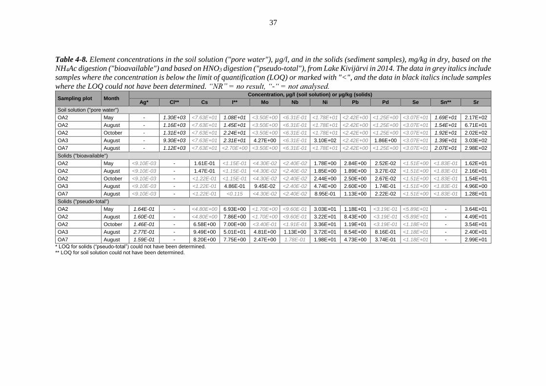
37
Table 4-8. Element concentrations in the soil solution ("pore water"), µg/l, and in the solids (sediment samples), mg/kg in dry, based on the
NH4Ac digestion ("bioavailable") and based on HNO3 digestion ("pseudo-total"), from Lake Kivijärvi in 2014. The data in grey italics include
samples where the concentration is below the limit of quantification (LOQ) or marked with "<", and the data in black italics include samples
where the LOQ could not have been determined. “NR” = no result, “-“ = not analysed.
Sampling plot Month Concentration, µg/l (soil solution) or µg/kg (solids)
Ag* Cl** Cs I** Mo Nb Ni Pb Pd Se Sn** Sr
Soil solution ("pore water")
OA2 May - 1.30E+03 <7.63E+01 1.08E+01 <3.50E+00 <6.31E-01 <1.78E+01 <2.42E+00 <1.25E+00 <3.07E+01 1.69E+01 2.17E+02
OA2 August - 1.16E+03 <7.63E+01 1.45E+01 <3.50E+00 <6.31E-01 <1.78E+01 <2.42E+00 <1.25E+00 <3.07E+01 1.54E+01 6.71E+01
OA2 October - 1.31E+03 <7.63E+01 2.24E+01 <3.50E+00 <6.31E-01 <1.78E+01 <2.42E+00 <1.25E+00 <3.07E+01 1.92E+01 2.02E+02
OA3 August - 9.30E+03 <7.63E+01 2.31E+01 4.27E+00 <6.31E-01 3.10E+02 <2.42E+00 1.86E+00 <3.07E+01 1.39E+01 3.03E+02
OA7 August - 1.12E+03 <7.63E+01 <2.70E+00 <3.50E+00 <6.31E-01 <1.78E+01 <2.42E+00 <1.25E+00 <3.07E+01 2.07E+01 2.98E+02
Solids ("bioavailable")
OA2 May <9.10E-03 - 1.61E-01 <1.15E-01 <4.30E-02 <2.40E-02 1.78E+00 2.84E+00 2.52E-02 <1.51E+00 <1.83E-01 1.62E+01
OA2 August <9.10E-03 - 1.47E-01 <1.15E-01 <4.30E-02 <2.40E-02 1.85E+00 1.89E+00 3.27E-02 <1.51E+00 <1.83E-01 2.16E+01
OA2 October <9.10E-03 - <1.22E-01 <1.15E-01 <4.30E-02 <2.40E-02 2.44E+00 2.50E+00 2.67E-02 <1.51E+00 <1.83E-01 1.54E+01
OA3 August <9.10E-03 - <1.22E-01 4.86E-01 9.45E-02 <2.40E-02 4.74E+00 2.60E+00 1.74E-01 <1.51E+00 <1.83E-01 4.96E+00
OA7 August <9.10E-03 - <1.22E-01 <0.115 <4.30E-02 <2.40E-02 8.95E-01 1.13E+00 2.22E-02 <1.51E+00 <1.83E-01 1.28E+01
Solids ("pseudo-total")
OA2 May 1.64E-01 - <4.80E+00 6.93E+00 <1.70E+00 <9.60E-01 3.03E+01 1.18E+01 <3.19E-01 <5.89E+01 - 3.64E+01
OA2 August 1.60E-01 - <4.80E+00 7.86E+00 <1.70E+00 <9.60E-01 3.22E+01 8.43E+00 <3.19E-01 <5.89E+01 - 4.49E+01
OA2 October 1.46E-01 - 6.58E+00 7.00E+00 <3.40E-01 <1.91E-01 3.36E+01 1.19E+01 <3.19E-01 <1.18E+01 - 3.54E+01
OA3 August 2.77E-01 - 9.49E+00 5.01E+01 4.81E+00 1.13E+00 3.72E+01 8.54E+00 8.16E-01 <1.18E+01 - 2.40E+01
OA7 August 1.59E-01 - 8.20E+00 7.75E+00 2.47E+00 1.78E-01 1.98E+01 4.73E+00 3.74E-01 <1.18E+01 - 2.99E+01
* LOQ for solids (“pseudo-total”) could not have been determined. ** LOQ for soil solution could not have been determined.

38
Table 4-9. The corresponding Kd values (mg/kg 105°-dry)/(µg/l) based on the NH4Ac digestion ("bioavailable") and based on HNO3 digestion
("pseudo-total"), from Lake Kivijärvi in 2014. The data in grey italics include samples where the concentration was below the limit of
quantification (LOQ) or marked with "<"; for these, the numerical value of LOQ/2 for soil solution and LOQ for solids are used as a
surrogate. The data in black italics include samples where the LOQ for soil solution could not have been determined. Kd values couldn’t be
calculated for elements Ag and Cl due to missing concentration analyzing results.
* LOQ for soil solution could not have been determined.
Sampling plot Month Calculated Kd values (µg/kg 105°C-dry)/(µg/l)
Cs I* Mo Nb Ni Pb Pd Se Sn* Sr
Solids ("bioavailable")
OA2 May 4.21 10.6 24.6 80.0 200 2 370 38.8 98.4 10.9 74.8
OA2 August 3.85 7.95 24.6 80.0 208 1 570 50.3 98.4 11.9 322
OA2 October 3.20 5.13 24.6 80.0 274 2 090 41.1 98.4 9.55 76.3
OA3 August 3.20 21.0 22.1 80.0 15.3 2 160 93.2 98.4 13.1 16.3
OA7 August 3.20 42.6 24.6 80.0 101 944 34.2 98.4 8.85 42.9
Solids ("pseudo-total")
OA2 May 126 641 971 3 200 3 410 9 840 491 3 840 42.4 168
OA2 August 126 543 971 3 200 3 620 7 030 491 3 840 46.6 669
OA2 October 172 312 194 637 3 780 9 920 491 769 37.3 175
OA3 August 249 2 160 1 130 3 750 120 7 110 438 769 51.3 79.2
OA7 August 215 2 870 1 410 638 2 230 3 940 575 769 34.6 100
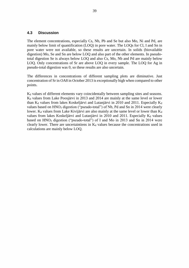
39
4.3 Discussion
The element concentrations, especially Cs, Nb, Pb and Se but also Mo, Ni and Pd, are
mainly below limit of quantification (LOQ) in pore water. The LOQs for Cl, I and Sn in
pore water were not available, so these results are uncertain. In solids (biovailable
digestion) Mo, Se and Sn are below LOQ and also part of the other elements. In pseudo-
total digestion Se is always below LOQ and also Cs, Mo, Nb and Pd are mainly below
LOQ. Only concentrations of Sr are above LOQ in every sample. The LOQ for Ag in
pseudo-total digestion was 0, so these results are also uncertain.
The differences in concentrations of different sampling plots are diminutive. Just
concentration of Sr in OA8 in October 2013 is exceptionally high when compared to other
points.
Kd values of different elements vary coincidentally between sampling sites and seasons.
Kd values from Lake Poosjärvi in 2013 and 2014 are mainly at the same level or lower
than Kd values from lakes Koskeljärvi and Lutanjärvi in 2010 and 2011. Especially Kd
values based on HNO3 digestion (“pseudo-total”) of Nb, Pd and Sn in 2014 were clearly
lower. Kd values from Lake Kivijärvi are also mainly at the same level or lower than Kd
values from lakes Koskeljärvi and Lutanjärvi in 2010 and 2011. Especially Kd values
based on HNO3 digestion (“pseudo-total”) of I and Mo in 2013 and Sn in 2014 were
clearly lower. There are uncertaintiens in Kd values because the concentrations used in
calculations are mainly below LOQ.

40

41
5 MACROPHYTES
Macrophytes were collected in Lakes Kivijärvi and Poosjärvi in May, August and
October 2013 (in Lake Poosjärvi only August and October due to spring floods in May
2013) and 2014 to establish the changes in the biomass and in the element inventories
during the growing season (Figure 5-1). Also, the database of typical dimensions and
weights of the plant individuals was executed for the assessments of radioecological
exposure of biota.
Figure 5-1. Sampling plots OA3 in Lake Kivijärvi (left, a-c) and OA12 in Lake Poosjärvi
(right, d-f) in May (top, a and d), August (middle, b and e) and October (bottom, c and f)
(photographs by Ville Kangasniemi and Ari Ikonen, EnviroCase Ltd., and Reija
Haapanen, Posiva Oy).
a.
b.
c.
d.
e.
f.
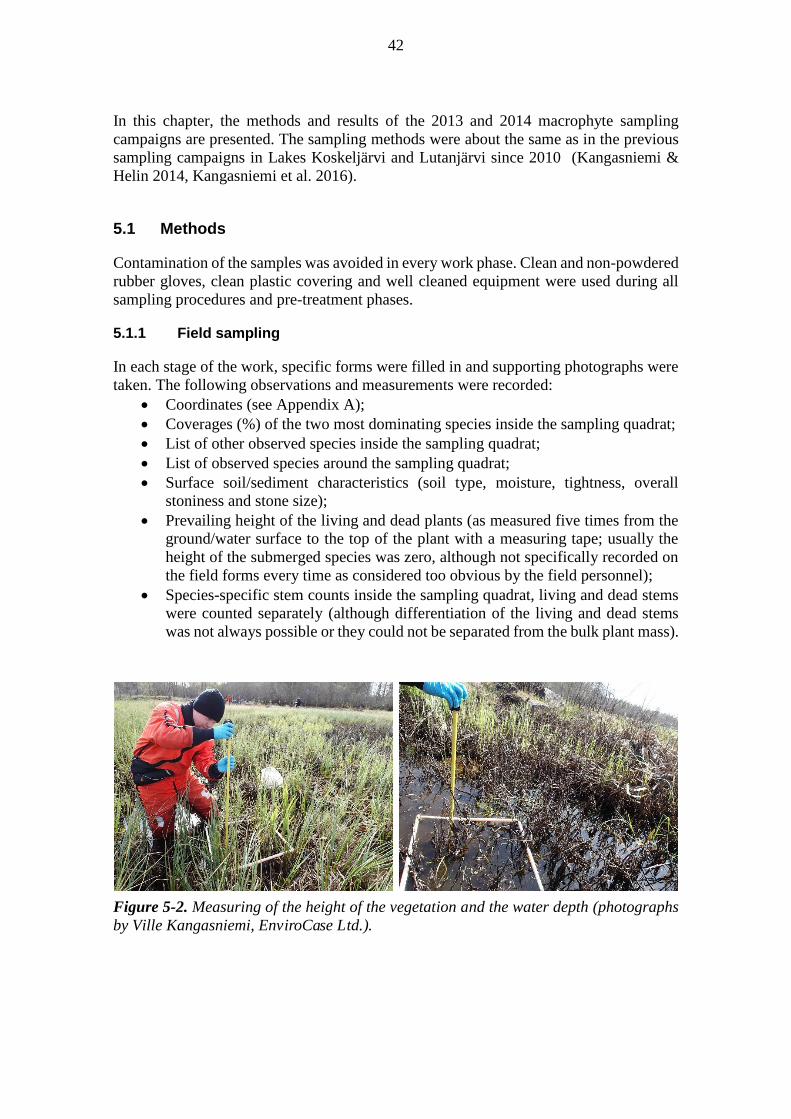
42
In this chapter, the methods and results of the 2013 and 2014 macrophyte sampling
campaigns are presented. The sampling methods were about the same as in the previous
sampling campaigns in Lakes Koskeljärvi and Lutanjärvi since 2010 (Kangasniemi &
Helin 2014, Kangasniemi et al. 2016).
5.1 Methods
Contamination of the samples was avoided in every work phase. Clean and non-powdered
rubber gloves, clean plastic covering and well cleaned equipment were used during all
sampling procedures and pre-treatment phases.
5.1.1 Field sampling
In each stage of the work, specific forms were filled in and supporting photographs were
taken. The following observations and measurements were recorded:
Coordinates (see Appendix A);
Coverages (%) of the two most dominating species inside the sampling quadrat;
List of other observed species inside the sampling quadrat;
List of observed species around the sampling quadrat;
Surface soil/sediment characteristics (soil type, moisture, tightness, overall
stoniness and stone size);
Prevailing height of the living and dead plants (as measured five times from the
ground/water surface to the top of the plant with a measuring tape; usually the
height of the submerged species was zero, although not specifically recorded on
the field forms every time as considered too obvious by the field personnel);
Species-specific stem counts inside the sampling quadrat, living and dead stems
were counted separately (although differentiation of the living and dead stems
was not always possible or they could not be separated from the bulk plant mass).
Figure 5-2. Measuring of the height of the vegetation and the water depth (photographs
by Ville Kangasniemi, EnviroCase Ltd.).
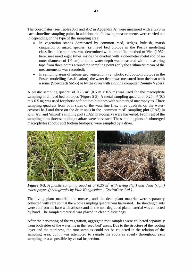
43
The coordinates (see Tables A-1 and A-2 in Appendix A) were measured with a GPS in
each shoreline sampling point. In addition, the following measurements were carried out
in depending on the type of the sampling area:
In vegetation stands dominated by common reed, sedges, bulrush, marsh
cinquefoil or mixed species (i.e., reed bed biotope in the Posiva modelling
classification): stoniness was determined with a modified method of Viro (1952;
here, measured eight times inside the quadrat with a one-metre metal rod of an
outer diameter of 1.0 cm), and the water depth was measured with a measuring
tape from three points around the sampling point (only the arithmetic mean of the
measurements was recorded);
In sampling areas of submerged vegetation (i.e., photic soft bottom biotope in the
Posiva modelling classification): the water depth was measured from the boat with
a sonar (Speedtech SM-5) or by the diver with a diving computer (Suunto Vyper).
A plastic sampling quadrat of 0.25 m² (0.5 m x 0.5 m) was used for the macrophyte
sampling in all reed bed biotopes (Figure 5-3). A metal sampling quadrat of 0.25 m² (0.5
m x 0.5 m) was used for photic soft bottom biotopes with submerged macrophytes. Three
sampling quadrats from both sides of the waterline (i.e., three quadrats on the water-
covered half and three on the drier one) in the ‘common reed’ sampling plot (OA3) in
Kivijärvi and ‘mixed’ sampling plot (OA5) in Poosjärvi were harvested. From rest of the
sampling plots three sampling quadrats were harvested. The sampling plots of submerged
macrophytes (photic soft bottom biotopes) were sampled by a diver.
Figure 5-3. A plastic sampling quadrat of 0.25 m2 with living (left) and dead (right)
macrophytes (photographs by Ville Kangasniemi, EnviroCase Ltd.).
The living plant material, the mosses, and the dead plant material were separately
collected with care so that the whole sampling quadrat was harvested. The standing plants
were cut from the base with scissors and all the non-degraded plant material was collected
by hand. The sampled material was placed in clean plastic bags.
After the harvesting of the vegetation, aggregate root samples were collected separately
from both sides of the waterline in the ‘reed bed’ areas. Due to the structure of the rooting
layer and the stoniness, the root samples could not be collected in the relation of the
sampling area, but it was attempted to sample the roots as evenly throughout each
sampling area as possible by visual inspection.
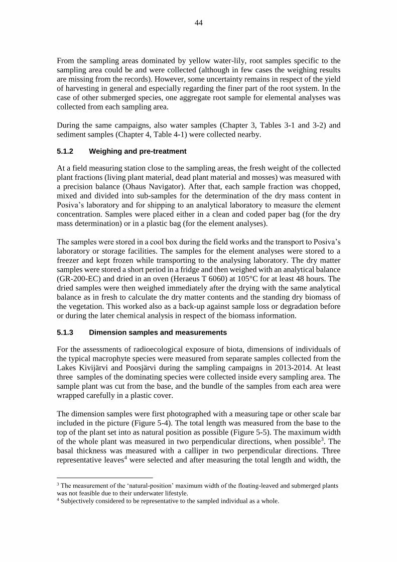
44
From the sampling areas dominated by yellow water-lily, root samples specific to the
sampling area could be and were collected (although in few cases the weighing results
are missing from the records). However, some uncertainty remains in respect of the yield
of harvesting in general and especially regarding the finer part of the root system. In the
case of other submerged species, one aggregate root sample for elemental analyses was
collected from each sampling area.
During the same campaigns, also water samples (Chapter 3, Tables 3-1 and 3-2) and
sediment samples (Chapter 4, Table 4-1) were collected nearby.
5.1.2 Weighing and pre-treatment
At a field measuring station close to the sampling areas, the fresh weight of the collected
plant fractions (living plant material, dead plant material and mosses) was measured with
a precision balance (Ohaus Navigator). After that, each sample fraction was chopped,
mixed and divided into sub-samples for the determination of the dry mass content in
Posiva’s laboratory and for shipping to an analytical laboratory to measure the element
concentration. Samples were placed either in a clean and coded paper bag (for the dry
mass determination) or in a plastic bag (for the element analyses).
The samples were stored in a cool box during the field works and the transport to Posiva’s
laboratory or storage facilities. The samples for the element analyses were stored to a
freezer and kept frozen while transporting to the analysing laboratory. The dry matter
samples were stored a short period in a fridge and then weighed with an analytical balance
(GR-200-EC) and dried in an oven (Heraeus T 6060) at 105°C for at least 48 hours. The
dried samples were then weighed immediately after the drying with the same analytical
balance as in fresh to calculate the dry matter contents and the standing dry biomass of
the vegetation. This worked also as a back-up against sample loss or degradation before
or during the later chemical analysis in respect of the biomass information.
5.1.3 Dimension samples and measurements
For the assessments of radioecological exposure of biota, dimensions of individuals of
the typical macrophyte species were measured from separate samples collected from the
Lakes Kivijärvi and Poosjärvi during the sampling campaigns in 2013-2014. At least
three samples of the dominating species were collected inside every sampling area. The
sample plant was cut from the base, and the bundle of the samples from each area were
wrapped carefully in a plastic cover.
The dimension samples were first photographed with a measuring tape or other scale bar
included in the picture (Figure 5-4). The total length was measured from the base to the
top of the plant set into as natural position as possible (Figure 5-5). The maximum width
of the whole plant was measured in two perpendicular directions, when possible3. The
basal thickness was measured with a calliper in two perpendicular directions. Three
representative leaves4 were selected and after measuring the total length and width, the
3 The measurement of the ‘natural-position’ maximum width of the floating-leaved and submerged plants
was not feasible due to their underwater lifestyle. 4 Subjectively considered to be representative to the sampled individual as a whole.
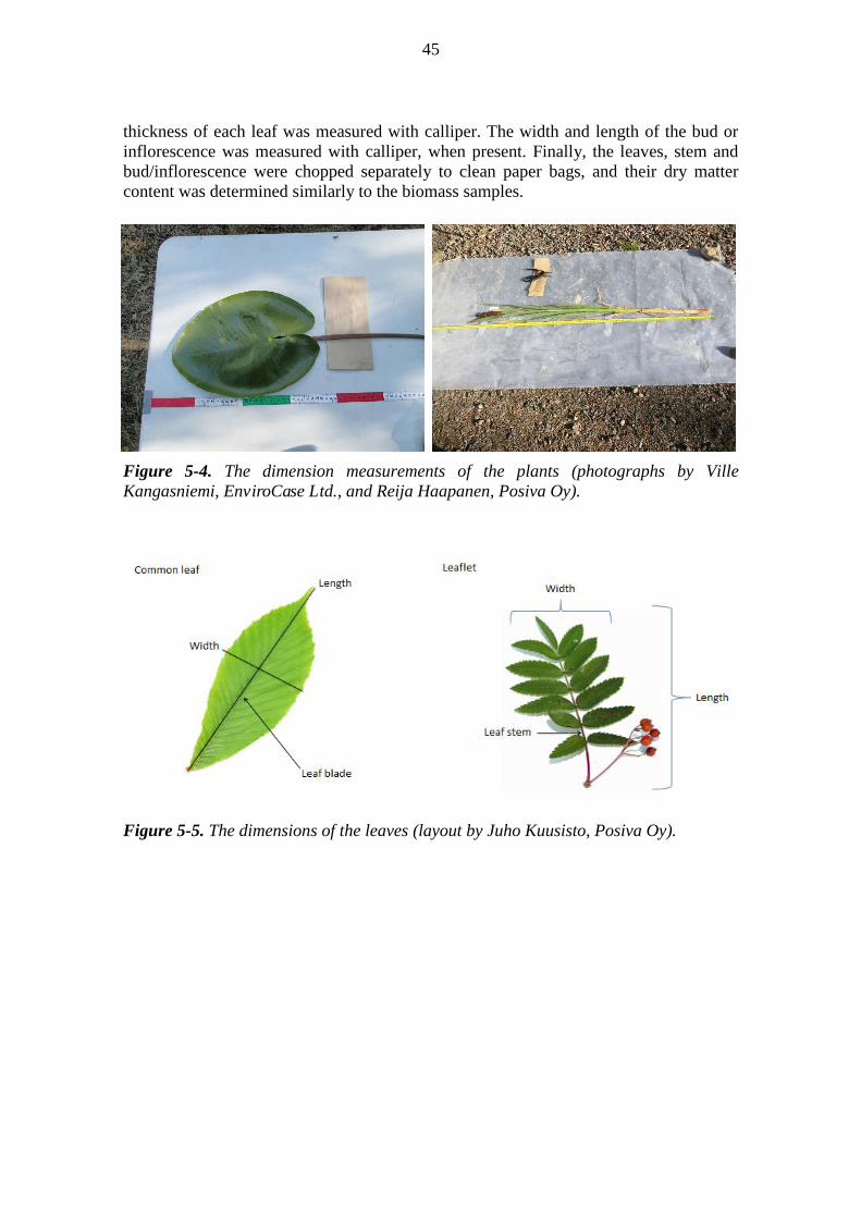
45
thickness of each leaf was measured with calliper. The width and length of the bud or
inflorescence was measured with calliper, when present. Finally, the leaves, stem and
bud/inflorescence were chopped separately to clean paper bags, and their dry matter
content was determined similarly to the biomass samples.
Figure 5-4. The dimension measurements of the plants (photographs by Ville
Kangasniemi, EnviroCase Ltd., and Reija Haapanen, Posiva Oy).
Figure 5-5. The dimensions of the leaves (layout by Juho Kuusisto, Posiva Oy).
46
5.1.4 Chemical analyses
All plant samples were analysed by the commercial laboratory ALS Scandinavia AB
(Sweden). The samples were dried at 50°C and digested with HNO3/HF (total digestion).
The element concentrations were then measured with an ICP-SFMS.
To remove aerial deposition, plant samples (although not all of them) have been initially
rinsed with MQ water before analysis. The samples were dried at 50°C before analysis.
Separate measurements of dry matter content at 105°C were carried out. Elemental
concentrations determined on material dried at 50°C were re-calculated and expressed on
dry matter content at 105°C basis. The dry matter content was carried out using freeze
drying.
Total element analysis after digestion with HNO3/HF(trace) was carried out for 70
elements by ICP-SFMS with methane addition to achieve the best possible LOQs for Ag
and Pd. All the elements were analysed quantitatively.
5.2 Results
General characteristics of the macrophyte sampling plots, including water depth, bottom
type, vegetation height and other observed species in each sampling plot, studied in Lakes
Kivijärvi and Poosjärvi in 2013 and 2014 are presented in Tables 5-1 to 5-4. Summary
statistics of the dimensions, weights (in dry) and dry matter proportions of the macrophyte
samples in Lakes Kivijärvi and Poosjärvi are presented in Tables 5-5 to 5-7.
Lakes Poosjärvi and Kivijärvi are rather shallow and the vegetation is abundant and dense
in both lakes. The assessment biotopes (table 3-1 in Posiva 2014) of the sampling plots
in Lake Poosjärvi are photic soft bottoms and reed beds, except the sampling plot OA4
which represents photic hard bottom. In Lake Kivijärvi the biotopes are photic soft
bottoms and reed beds. The dominating species in the sampling plots of Lake Poosjärvi
are horsetail (Equisetum), yellow water-lily (Nuphar lutea), floating pondweed
(Potamogeton natans), bulrush (Typha), sedges (Cyperaceae) and marsh cinquefoil
(Comarum palustre). The dominating species in the sampling plots of Lake Kivijärvi are
yellow water-lily (Nuphar lutea), common reed (Phragmites australis), bulrush (Typha)
and sedges (Cyperaceae).
The two years (2013-2014) mean biomasses of living bryophytes, living other vegetation
and dead vegetation in Lakes Kivijärvi and Poosjärvi in May, August and October are
presented in Figures 5-1 to 5-3. The mean biomasses of living vegetation were naturally
highest in August. The biomass of dead vegetation varied between biotopes randomly.
The highest biomass of dead vegetation was observed in May in sampling plot OA6 in
Poosjärvi, where floating pondweed is the dominating species. The statistics of fresh and
dry biomass and dry matter content for all the sampling plots are present in Appendix D.
The concentrations of the key elements and their rank order for each dominating species
(living parts) in August 2013 and August 2014 are presented in Tables 5-8 and 5-9. The
concentarations of Cl, Se, Ni and I are highest and concentrations of Ag and Pd are lowest

47
in each species in 2013 and 2014. The concentrations of all the analysed elements in lake
water and in plants from all sampling plots and every sampling date are presented in
Appendix D.
The water-to-plant concentration ratios (including the living parts of the dominating
species) in August 2013 and 2014 from Lake Poosjärvi are presented in Figure 5-4 and
from Lake Kivijärvi in Figure 5-5. The water-to-plant concentration ratios of the elements
vary considerably between sampling plots in both lakes. The annual variation is wide
especially in concentration ratios of Ag, Nb, Pb, Pd and Sn, and specially in sampling
plots OA6 (floating pondweed) and OA7 (horsetail) in Lake Poosjärvi. The annual
variation is clear in concentration ratios of Ag, Nb, Pd, Se and Sn in Lake Kivijärvi.The
annual variation in concentration ratios of Pd is exceptionally wide in every sampling plot
in both lakes. In general the water-to-plant concentration ratios are lower in Lake
Kivijärvi than in Lake Poosjärvi.
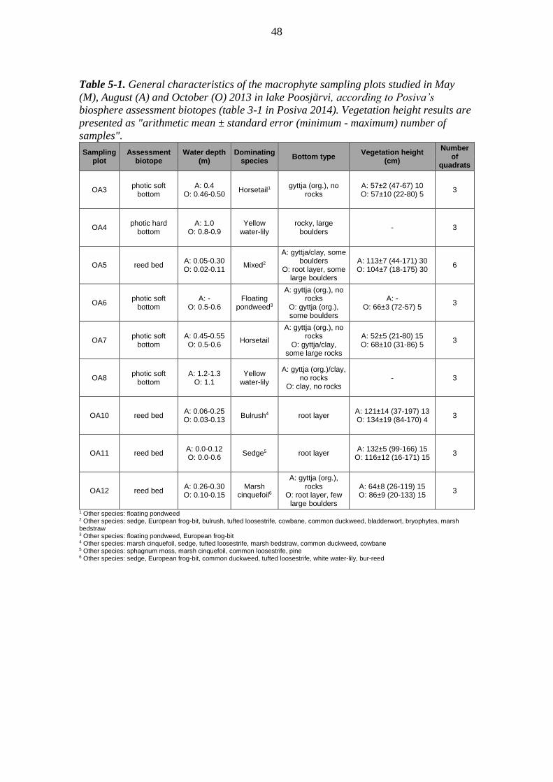
48
Table 5-1. General characteristics of the macrophyte sampling plots studied in May
(M), August (A) and October (O) 2013 in lake Poosjärvi, according to Posiva’s
biosphere assessment biotopes (table 3-1 in Posiva 2014). Vegetation height results are
presented as "arithmetic mean ± standard error (minimum - maximum) number of
samples".
Sampling plot
Assessment biotope
Water depth (m)
Dominating species
Bottom type Vegetation height
(cm)
Number of
quadrats
OA3 photic soft
bottom A: 0.4
O: 0.46-0.50 Horsetail1 gyttja (org.), no
rocks A: 57±2 (47-67) 10 O: 57±10 (22-80) 5
3
OA4 photic hard
bottom A: 1.0
O: 0.8-0.9 Yellow
water-lily rocky, large
boulders - 3
OA5 reed bed A: 0.05-0.30 O: 0.02-0.11
Mixed2
A: gyttja/clay, some boulders
O: root layer, some large boulders
A: 113±7 (44-171) 30 O: 104±7 (18-175) 30
6
OA6 photic soft
bottom A: -
O: 0.5-0.6 Floating
pondweed3
A: gyttja (org.), no rocks
O: gyttja (org.), some boulders
A: - O: 66±3 (72-57) 5
3
OA7 photic soft
bottom A: 0.45-0.55 O: 0.5-0.6
Horsetail
A: gyttja (org.), no rocks
O: gyttja/clay, some large rocks
A: 52±5 (21-80) 15 O: 68±10 (31-86) 5
3
OA8 photic soft
bottom A: 1.2-1.3
O: 1.1 Yellow
water-lily
A: gyttja (org.)/clay, no rocks
O: clay, no rocks - 3
OA10 reed bed A: 0.06-0.25 O: 0.03-0.13
Bulrush4 root layer A: 121±14 (37-197) 13 O: 134±19 (84-170) 4
3
OA11 reed bed A: 0.0-0.12 O: 0.0-0.6
Sedge5 root layer A: 132±5 (99-166) 15
O: 116±12 (16-171) 15 3
OA12 reed bed A: 0.26-0.30 O: 0.10-0.15
Marsh cinquefoil6
A: gyttja (org.), rocks
O: root layer, few large boulders
A: 64±8 (26-119) 15 O: 86±9 (20-133) 15
3
1 Other species: floating pondweed 2 Other species: sedge, European frog-bit, bulrush, tufted loosestrife, cowbane, common duckweed, bladderwort, bryophytes, marsh bedstraw 3 Other species: floating pondweed, European frog-bit 4 Other species: marsh cinquefoil, sedge, tufted loosestrife, marsh bedstraw, common duckweed, cowbane 5 Other species: sphagnum moss, marsh cinquefoil, common loosestrife, pine 6 Other species: sedge, European frog-bit, common duckweed, tufted loosestrife, white water-lily, bur-reed

49
Table 5-2. General characteristics of the macrophyte sampling plots studied in May (M),
August (A) and October (O) 2014 in lake Poosjärvi, according to Posiva’s biosphere
assessment biotopes (table 3-1 in Posiva 2014). Vegetation height results are presented
as "arithmetic mean ± standard error (minimum - maximum) number of samples".
1 Other species: yellow water-lily 2 Other species: sedge, common duckweed, tufted loosestrife, marsh bedstraw, calliergon moss; additionally next to the sampling quadrats willow, bulrush, cowbane, purple small-reed, common loosestrife, flatleaf bladderwort, purple loosestrife, sphagnum moss, milk-parsley, amphibious bistort 3 Other species: horsetail 4 Other species: yellow water-lily; additionally next to the sampling quadrats white water-lily 5 Other species: next to the sampling quadrats horsetail 6 Other species: sedge, marsh cinquefoil, sphagnum moss, common duckweed, European frog-bit, marsh bedstraw, milk-parsley, tufted loosestrife, calliergon moss, purple loosestrife, common loosestrife; additionally next to the sampling quadrats willow, alder, yellow water-lily, bladderwort, cowbane, bulrush 7 Other species: marsh cinquefoil, sphagnum moss, marsh bedstraw; additionally next to the sampling quadrats birch, willow, sphagnum moss, bulrush, tufted loosestrife, bog arum 8 Other species: sedge, bog bean, European frog-bit, common duckweed, tufted loosestrife, marsh bedstraw; additionally next to the sampling quadrats yellow water-lily, calliergon moss, bur-reed, bulrush, purple loosestrife, bladderwort, cowbane, alder, willow
Sampling plot
Assessment biotope
Water depth (m)
Dominating species
Bottom type Vegetation height
(cm)
Number of
quadrats
OA1 reed bed - Sedge - - 3
OA2 reed bed - Bulrush - - 3
OA3 photic soft
bottom
M: 0.7 A: 0.4-0.5
O: - Horsetail1
M: gyttja/clay, no rocks A: gyttja (org.), no rocks
O: gyttja/clay, some small boulders
M: 13±3 (2-21) 5 A: 49±8 (18-65) 5 O: 54±14 (17-238) 15
3
OA4 photic hard
bottom
M: 1.1-1.2 A: 1.0-1.3 O: 1.1-1.2
Yellow water-lily
rocky, lots of boulders - 3
OA5 reed bed
M: 0.0-0.14 A: 0.01-0.08
O: 0.03-0.12
Mixed (bog arum,
marsh cinquefoil)2
M: gyttja/clay, boulders A: gyttja/clay/gravel,
boulders O: gyttja/clay, boulders
M: 48±4 (12-83) 30 A: 97±4 (63-156) 30 O: 56±5 (7-129) 30
6
OA6 photic soft
bottom
M: 0.8 A: 0.5
O: 0.6-0.7
Floating pondweed3
M: gyttja/clay, no rocks A: gyttja (org.), no rocks O: gyttja/clay, no rocks
M: - A: 40
O: 48±4 (21-69) 15 3
OA7 photic soft
bottom
M: 0.7 A: 0.4
O: 0.4-0.5 Horsetail4
M: gyttja/clay, some large boulders
A: gyttja (org.), some boulders
O: gyttja/clay, no rocks
M: 18±5 (2-29) 5 A: 65±6 (43-89) 10 O: 64±5 (21-92) 15
3
OA8 photic soft
bottom
M: 1.2 A: 1.0-1.2 O: 1.2-1.3
Yellow water-lily5
M: gyttja/clay, no rocks A: gyttja/clay, no rocks O: gyttja/clay, no rocks
- 3
OA10 reed bed
M: 0.04-0.20
A: 0.0-0.09 O: 0.04-
0.08
Bulrush6
M: gyttja/clay, no rocks A: gyttja (org.), no rocks O: gyttja/clay, no rocks
M: 43±3 (27-65) 15 A: 156±5 (129-190)
15 O: 84±17 (12-213)
15
3
OA11 reed bed
M: 0.01-0.04 A: 0.0-0.03 O: 0.0-
0.03
Sedge7
M: gyttja/clay, no rocks A: gyttja/clay, no rocks O: gyttja/clay, no rocks
M: 43±2 (31-58) 15 A: 88±4 (53-114) 15 O: 42±4 (20-71) 15
3
OA12 reed bed
M: 0.14-0.46 A:
0.04-0.42 O: 0.09-
0.25
Marsh cinquefoil8
M: gyttja/clay, boulders A:
gyttja/clay/sand/gravel, boulders
O: gyttja/clay, some large boulders
M: 53±6 (13-80) 15 A: 86±6 (57-150) 15 O: 42±7 (8-80) 15
3
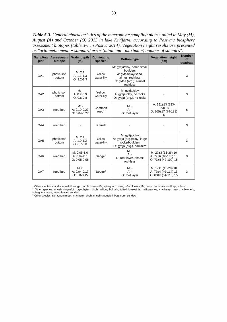
50
Table 5-3. General characteristics of the macrophyte sampling plots studied in May (M),
August (A) and October (O) 2013 in lake Kivijärvi, according to Posiva’s biosphere
assessment biotopes (table 3-1 in Posiva 2014). Vegetation height results are presented
as "arithmetic mean ± standard error (minimum - maximum) number of samples".
Sampling plot
Assessment biotope
Water depth (m)
Dominating species
Bottom type Vegetation height
(cm)
Number of
quadrats
OA1 photic soft
bottom
M: 2.1 A: 1.1-1.3 O: 1.2-1.3
Yellow water-lily
M: gyttja/clay, some small boulders
A: gyttja/clay/sand, almost rockless
O: gyttja (org.), almost rockless
- 3
OA2 photic soft
bottom
M: - A: 0.7-0.9 O: 0.6-0.8
Yellow water-lily
M: gyttja/clay A: gyttja/clay, no rocks
O: gyttja (org.), no rocks - 3
OA3 reed bed M: -
A: 0.10-0.27 O: 0.04-0.27
Common reed1
M: - A: -
O: root layer
A: 251±13 (133-373) 30
O: 105±17 (74-188) 6
6
OA4 reed bed - Bulrush - - 3
OA5 photic soft
bottom
M: 2.1 A: 1.0-1.2 O: 0.7-0.8
Yellow water-lily
M: gyttja/clay A: gyttja (org.)/clay, large
rocks/boulders O: gyttja (org.), boulders
- 3
OA6 reed bed M: 0.05-1.0 A: 0.07-0.1
O: 0.05-0.06 Sedge2
M: - A: -
O: root layer, almost rockless
M: 27±3 (13-36) 10 A: 79±6 (40-113) 15 O: 73±5 (42-109) 15
3
OA7 reed bed M: 0
A: 0.04-0.17 O: 0.0-0.15
Sedge3
M: - A: -
O: root layer
M: 17±1 (13-20) 10 A: 79±4 (49-114) 15 O: 83±6 (51-110) 15
3
1 Other species: marsh cinquefoil, sedge, purple loosestrife, sphagnum moss, tufted loosestrife, marsh bedstraw, skullcap, bulrush 2 Other species: marsh cinquefoil, bryophytes, birch, willow, bulrush, tufted loosestrife, milk-parsley, cranberry, marsh willowherb, sphagnum moss, round-leaved sundew 3 Other species: sphagnum moss, cranberry, birch, marsh cinquefoil, bog arum, sundew

51
Table 5-4. General characteristics of the macrophyte sampling plots studied in May (M),
August (A) and October (O) 2014 in lake Kivijärvi, according to Posiva’s biosphere
assessment biotopes (table 3-1 in Posiva 2014). Vegetation height results are presented
as "arithmetic mean ± standard error (minimum - maximum) number of samples".
Sampling plot
Assessment biotope
Water depth (m)
Dominating species
Bottom type Vegetation height
(cm)
Number of
quadrats
OA1 photic soft
bottom
M: 1.3-1.4 A: 1.2 O: 1.2
Yellow water-lily
M: gyttja/clay, few small boulders
A: gyttja/clay, almost rockless
O: gyttja/ clay, no rocks
M: - A: 5 O: -
3
OA2 photic soft
bottom M: 1.0-1.2 A: 0.7-1.0
Yellow water-lily
M: gyttja/clay, no rocks A: gyttja/clay, almost
rockless O: gyttja/ clay, no rocks
M: - A: -
3
OA3 reed bed M: 0.01-0.22 A: 0.05-0.15 O: 0.0-0.17
Common reed1
M: peat layer, no rocks/few boulders A: gravel, few small
boulders O: -, no rocks
M: 41±3 (11-84) 30 A: 196±14 (60-340)
30 O: 61±11 (16-160) 20
6
OA4 reed bed - Bulrush - - 3
OA5 photic soft
bottom
M: 0.6-0.7 A: 0.6-0.8
O: 0.01-0.03
Yellow water-lily
M: gyttja (org.)/clay, few boulders
A: gyttja/clay, few boulders
O: gyttja/clay, some small boulders
M: - A: 5 O: -
3
OA6 reed bed M: 0.08-0.09 A: 0.01-0.05 O: 0.0-0.07
Sedge2
M: peat layer/gyttja (org.), no rocks/few
boulders A: gravel, large rocks
O: gyttja/clay/sand/gravel,
few large boulders
M: 38±2 (27-49) 15 A: 68±6 (8-100) 15 O: 47±5 (18-85) 15
3
OA7 reed bed M: 0.0-0.005 A: 0.0-0.05
O: 0 Sedge3
M: peat layer, no rocks A: gyttja (org.), no
rocks O: -, no rocks
M: 32±2 (17-43) 15 A: 74±5 (33-101) 15 O: 41±5 (10-63) 15
3
1 Other species: sedge, marsh cinquefoil, bulrush, purple loosestrife, sphagnum moss, marsh bedstraw, common loosestrife, marsh willowherb, gypsywort, skullcap, tufted loosestrife, cowbane, European frog-bit, milk-parsley, common duckweed, calliergon moss 2 Other species: sphagnum moss, marsh cinquefoil, calliergon moss, round-leaved sundew, tufted loosestrife, bulrush, cranberry 3 Other species: cranberry, sphagnum moss, birch, round-leaved sundew
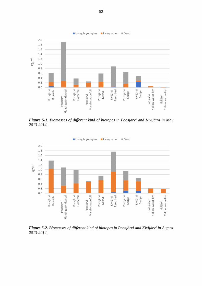
52
0,0
0,2
0,4
0,6
0,8
1,0
1,2
1,4
1,6
1,8
2,0
Po
osj
ärvi
Bu
lru
sh
Po
osj
ärvi
Flo
atin
g p
on
dw
eed
Po
osj
ärvi
Ho
rset
ail
Po
osj
ärvi
Mar
sh c
inq
uef
oil
Po
osj
ärvi
Mix
ed
Kiv
ijärv
iR
eed
be
d
Po
osj
ärvi
Sed
ge
Kiv
ijärv
iSe
dge
Po
osj
ärvi
Yello
w w
ater
-lily
Kiv
ijärv
iYe
llow
wat
er-l
ily
kg/m
²
Living bryophytes Living other Dead
0,0
0,2
0,4
0,6
0,8
1,0
1,2
1,4
1,6
1,8
2,0
Po
osj
ärvi
Bu
lru
sh
Po
osj
ärvi
Flo
atin
g p
on
dw
eed
Po
osj
ärvi
Ho
rset
ail
Po
osj
ärvi
Mar
sh c
inq
uef
oil
Po
osj
ärvi
Mix
ed
Kiv
ijärv
iR
eed
be
d
Po
osj
ärvi
Sed
ge
Kiv
ijärv
iSe
dge
Po
osj
ärvi
Yello
w w
ater
-lily
Kiv
ijärv
iYe
llow
wat
er-l
ily
kg/m
²Living bryophytes Living other Dead
Figure 5-1. Biomasses of different kind of biotopes in Poosjärvi and Kivijärvi in May
2013-2014.
Figure 5-2. Biomasses of different kind of biotopes in Poosjärvi and Kivijärvi in August
2013-2014.
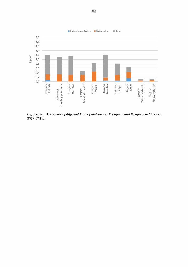
53
Figure 5-3. Biomasses of different kind of biotopes in Poosjärvi and Kivijärvi in October
2013-2014.
0,0
0,2
0,4
0,6
0,8
1,0
1,2
1,4
1,6
1,8
2,0
Po
osj
ärvi
Bu
lru
sh
Po
osj
ärvi
Flo
atin
g p
on
dw
eed
Po
osj
ärvi
Ho
rset
ail
Po
osj
ärvi
Mar
sh c
inq
uef
oil
Po
osj
ärvi
Mix
ed
Kiv
ijärv
iR
eed
be
d
Po
osj
ärvi
Sed
ge
Kiv
ijärv
iSe
dge
Po
osj
ärvi
Yello
w w
ater
-lily
Kiv
ijärv
iYe
llow
wat
er-l
ily
kg/m
²Living bryophytes Living other Dead
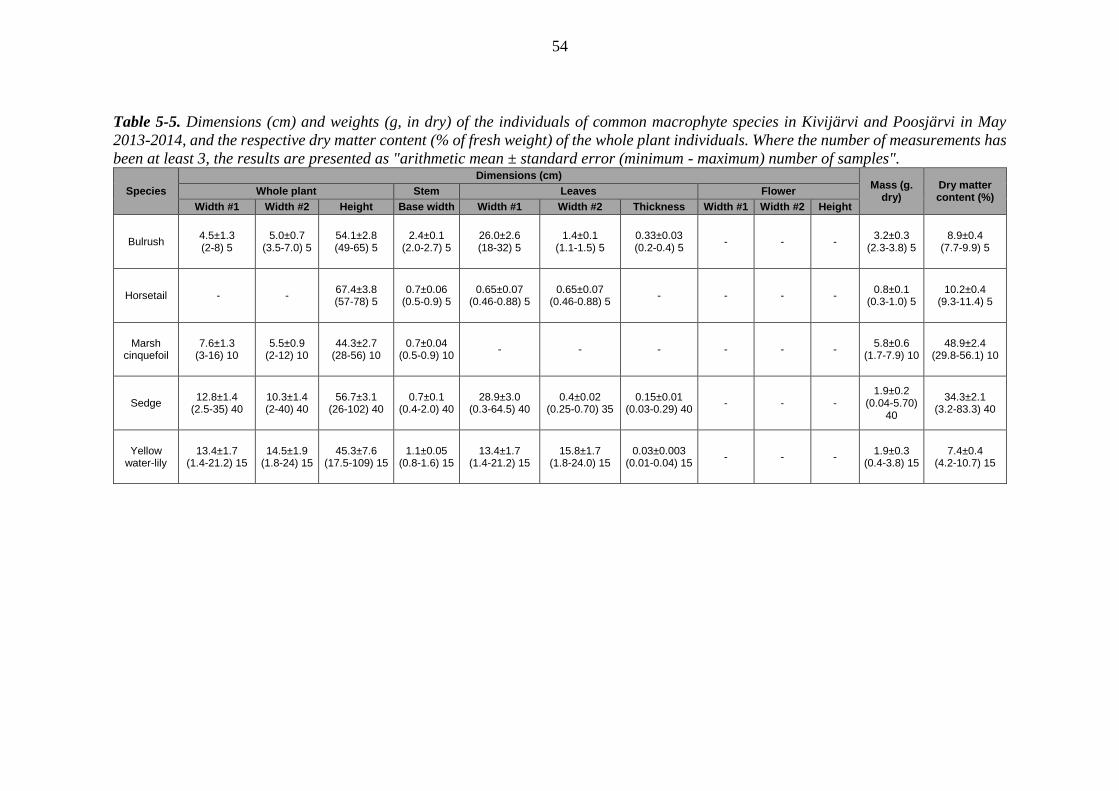
54
Table 5-5. Dimensions (cm) and weights (g, in dry) of the individuals of common macrophyte species in Kivijärvi and Poosjärvi in May
2013-2014, and the respective dry matter content (% of fresh weight) of the whole plant individuals. Where the number of measurements has
been at least 3, the results are presented as "arithmetic mean ± standard error (minimum - maximum) number of samples".
Species
Dimensions (cm) Mass (g.
dry) Dry matter content (%)
Whole plant Stem Leaves Flower
Width #1 Width #2 Height Base width Width #1 Width #2 Thickness Width #1 Width #2 Height
Bulrush 4.5±1.3 (2-8) 5
5.0±0.7 (3.5-7.0) 5
54.1±2.8 (49-65) 5
2.4±0.1 (2.0-2.7) 5
26.0±2.6 (18-32) 5
1.4±0.1 (1.1-1.5) 5
0.33±0.03 (0.2-0.4) 5
- - - 3.2±0.3
(2.3-3.8) 5 8.9±0.4
(7.7-9.9) 5
Horsetail - - 67.4±3.8 (57-78) 5
0.7±0.06 (0.5-0.9) 5
0.65±0.07 (0.46-0.88) 5
0.65±0.07 (0.46-0.88) 5
- - - - 0.8±0.1
(0.3-1.0) 5 10.2±0.4
(9.3-11.4) 5
Marsh cinquefoil
7.6±1.3 (3-16) 10
5.5±0.9 (2-12) 10
44.3±2.7 (28-56) 10
0.7±0.04 (0.5-0.9) 10
- - - - - - 5.8±0.6
(1.7-7.9) 10 48.9±2.4
(29.8-56.1) 10
Sedge 12.8±1.4
(2.5-35) 40 10.3±1.4 (2-40) 40
56.7±3.1 (26-102) 40
0.7±0.1 (0.4-2.0) 40
28.9±3.0 (0.3-64.5) 40
0.4±0.02 (0.25-0.70) 35
0.15±0.01 (0.03-0.29) 40
- - - 1.9±0.2
(0.04-5.70) 40
34.3±2.1 (3.2-83.3) 40
Yellow water-lily
13.4±1.7 (1.4-21.2) 15
14.5±1.9 (1.8-24) 15
45.3±7.6 (17.5-109) 15
1.1±0.05 (0.8-1.6) 15
13.4±1.7 (1.4-21.2) 15
15.8±1.7 (1.8-24.0) 15
0.03±0.003 (0.01-0.04) 15
- - - 1.9±0.3
(0.4-3.8) 15 7.4±0.4
(4.2-10.7) 15

55
Table 5-6. Dimensions (cm) and weights (g, in dry) of the individuals of common macrophyte species in Kivijärvi and Poosjärvi in August
2013-2014, and the respective dry matter content (% of fresh weight) of the whole plant individuals. Where the number of measurements has
been at least 3, the results are presented as "arithmetic mean ± standard error (minimum - maximum) number of samples".
Species
Dimensions (cm) Mass (g.
dry)
Dry matter content
(%) Whole plant Stem Leaves Flower
Width #1 Width #2 Height Base width Width #1 Width #2 Thickness Width #1 Width #2 Height
Bulrush 29.1±2.7
(12-55) 20 23.7±3.2 (4-53) 20
160±5 (111-201)
20
2.5±0.1 (1.5-3.2) 20
78.7±2.4 (56 -101) 20
1.7±0.1 (1.3-2.2) 20
0.23±0.01 (0.16-0.43) 20
2.8±0.1 (1.9-3.4) 20
2.7±0.1 (1.9-3.4) 20
23.9±1.8 (11-40) 20
75±6 (23-117) 20
26.3±0.6 (21.1-30.6)
20
Common reed
44.2±6.7 (19-75) 10
24.7±4.4 (6-54) 10
256±19 (181-346)
10
0.8±0.1 (0.5-1.1) 10
2.0±0.4 (0.4-3.7) 10
40.6±1.9 (33.3-50.7)
10
0.21±0.06 (0.03-0.52) 10
9.6±1.3 (2.5-16) 10
9.5±1.2 (4-16) 10
24.4±1.2 (19-30) 10
22.3±2.6 (6.9-32.4)
10
46.1±1.8 (39.7-55.9)
10
Floating pondweed
9.8±1.2 (8-14) 5
11±1.4 (7-15) 5
79±5 (67-90) 5
0.23±0.03 (0.15-0.31) 5
2.8±0.2 (2.2-3.2) 5
5.6±0.5 (4.0-6.9) 5
0.021±0.001 (0.020-0.023) 5
1.1 0.7 6.5 2.3±0.4
(0.8-3.0) 5
14.7±2.3 (12.3-24.9)
5
Horsetail 5.9±1.0
(0.5-21.0) 24
5.6±0.8 (0.5-14.5)
24
95±5 (52-129)
24
0.6±0.02 (0.4-0.9) 24
3.5±1.2 (0.03-18.7)
21
5.2±1.5 (0.01-19.5)
21
2.1±0.9 (0.01-12.4) 21
- - - 2.1±0.1
(1.0-3.3) 24
24.0±1.2 (15.7-33.3)
24
Bog arum 31.8±4.9
(18-69) 10 21.5±2.2
(10-37) 10 53.6±4.0
(34-75) 10 3.3±1.5
(1.1-17) 10
10.5±0.7 (7.7-14.6)
10
12.3±0.7 (9.3-16.3) 10
0.02±0.004 (0.01-0.04) 10
1.7 1.8 3.4 11.1±1.7
(3.4-21) 10
12.4±1.0 (8.5-17.4)
10
Marsh cinquefoil
21.1±1.8 (6-35) 20
17.9±1.3 (8.5-27) 20
65.9±3.9 (30-105)
20
0.6±0.02 (0.4-0.8) 20
4.7±0.5 (2.0-8.4) 20
5.1±0.8 (1.4-10.7) 20
0.14±0.04 (0.02-0.57) 20
5.0±1.0 (2.4-11) 10
3.4±0.5 (1.6-7.0) 10
8.5±3.0 (2.8-32) 10
8.9±0.7 (2.3-13.5)
20
34.6±2.5 (22.4-70.4)
20
Sedge 22.8±2.5 (3-65) 30
21.4±1.8 (6-39) 30
102±7 (46-175)
30
0.7±0.1 (0.3-1.7) 30
58.8±4.5 (32-118) 30
0.40±0.03 (0.23-0.75)
30
0.24±0.01 (0.15-0.37) 30
0.6±0.1 (0.3-1.0) 14
0.6±0.1 (0.4-1.0) 14
11.4±2.5 (2.8-29) 14
3.9±0.3 (0.6-7.5) 30
36.3±1.7 (25.4-61.6)
30
Yellow water-lily
19.4±1.7 (2.1-28) 20
25.3±2.3 (2.1-37) 20
139±6 (49-178)
20
1.1±0.04 (0.8-1.4) 20
22.2±0.9 (15-28) 17
29.1±1.1 (21-37) 17
0.07±0.01 (0.01-0.10) 17
3.7±0.8 (2.1-4.9) 3
3.8±0.9 (2.1-5.1) 3
3.7±1.1 (1.7-5.5) 3
8.1±0.7 (1.7-12.6)
20
12.3±1.0 (4.5-19.2)
20
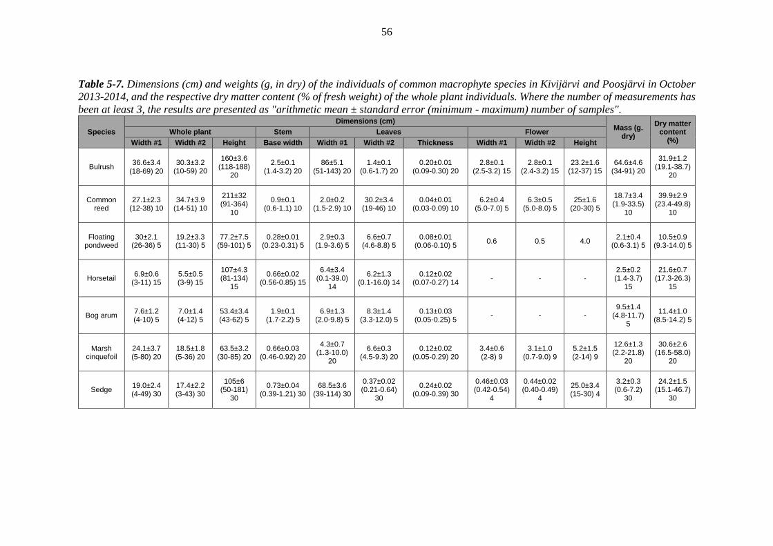
56
Table 5-7. Dimensions (cm) and weights (g, in dry) of the individuals of common macrophyte species in Kivijärvi and Poosjärvi in October
2013-2014, and the respective dry matter content (% of fresh weight) of the whole plant individuals. Where the number of measurements has
been at least 3, the results are presented as "arithmetic mean ± standard error (minimum - maximum) number of samples".
Species
Dimensions (cm) Mass (g.
dry)
Dry matter content
(%) Whole plant Stem Leaves Flower
Width #1 Width #2 Height Base width Width #1 Width #2 Thickness Width #1 Width #2 Height
Bulrush 36.6±3.4
(18-69) 20
30.3±3.2 (10-59) 20
160±3.6 (118-188)
20
2.5±0.1 (1.4-3.2) 20
86±5.1 (51-143) 20
1.4±0.1 (0.6-1.7) 20
0.20±0.01 (0.09-0.30) 20
2.8±0.1 (2.5-3.2) 15
2.8±0.1 (2.4-3.2) 15
23.2±1.6 (12-37) 15
64.6±4.6 (34-91) 20
31.9±1.2 (19.1-38.7)
20
Common reed
27.1±2.3 (12-38) 10
34.7±3.9 (14-51) 10
211±32 (91-364)
10
0.9±0.1 (0.6-1.1) 10
2.0±0.2 (1.5-2.9) 10
30.2±3.4 (19-46) 10
0.04±0.01 (0.03-0.09) 10
6.2±0.4 (5.0-7.0) 5
6.3±0.5 (5.0-8.0) 5
25±1.6 (20-30) 5
18.7±3.4 (1.9-33.5)
10
39.9±2.9 (23.4-49.8)
10
Floating pondweed
30±2.1 (26-36) 5
19.2±3.3 (11-30) 5
77.2±7.5 (59-101) 5
0.28±0.01 (0.23-0.31) 5
2.9±0.3 (1.9-3.6) 5
6.6±0.7 (4.6-8.8) 5
0.08±0.01 (0.06-0.10) 5
0.6 0.5 4.0 2.1±0.4
(0.6-3.1) 5 10.5±0.9
(9.3-14.0) 5
Horsetail 6.9±0.6
(3-11) 15 5.5±0.5 (3-9) 15
107±4.3 (81-134)
15
0.66±0.02 (0.56-0.85) 15
6.4±3.4 (0.1-39.0)
14
6.2±1.3 (0.1-16.0) 14
0.12±0.02 (0.07-0.27) 14
- - - 2.5±0.2 (1.4-3.7)
15
21.6±0.7 (17.3-26.3)
15
Bog arum 7.6±1.2 (4-10) 5
7.0±1.4 (4-12) 5
53.4±3.4 (43-62) 5
1.9±0.1 (1.7-2.2) 5
6.9±1.3 (2.0-9.8) 5
8.3±1.4 (3.3-12.0) 5
0.13±0.03 (0.05-0.25) 5
- - - 9.5±1.4
(4.8-11.7) 5
11.4±1.0 (8.5-14.2) 5
Marsh cinquefoil
24.1±3.7 (5-80) 20
18.5±1.8 (5-36) 20
63.5±3.2 (30-85) 20
0.66±0.03 (0.46-0.92) 20
4.3±0.7 (1.3-10.0)
20
6.6±0.3 (4.5-9.3) 20
0.12±0.02 (0.05-0.29) 20
3.4±0.6 (2-8) 9
3.1±1.0 (0.7-9.0) 9
5.2±1.5 (2-14) 9
12.6±1.3 (2.2-21.8)
20
30.6±2.6 (16.5-58.0)
20
Sedge 19.0±2.4 (4-49) 30
17.4±2.2 (3-43) 30
105±6 (50-181)
30
0.73±0.04 (0.39-1.21) 30
68.5±3.6 (39-114) 30
0.37±0.02 (0.21-0.64)
30
0.24±0.02 (0.09-0.39) 30
0.46±0.03 (0.42-0.54)
4
0.44±0.02 (0.40-0.49)
4
25.0±3.4 (15-30) 4
3.2±0.3 (0.6-7.2)
30
24.2±1.5 (15.1-46.7)
30
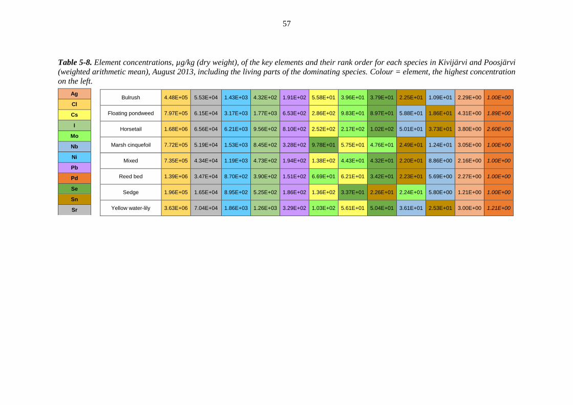
57
Table 5-8. Element concentrations, µg/kg (dry weight), of the key elements and their rank order for each species in Kivijärvi and Poosjärvi
(weighted arithmetic mean), August 2013, including the living parts of the dominating species. Colour = element, the highest concentration
on the left.
Ag
Cl
Cs
I
Mo
Nb
Ni
Pb
Pd
Se
Sn
Sr
Bulrush 4.48E+05 5.53E+04 1.43E+03 4.32E+02 1.91E+02 5.58E+01 3.96E+01 3.79E+01 2.25E+01 1.09E+01 2.29E+00 1.00E+00
Floating pondweed 7.97E+05 6.15E+04 3.17E+03 1.77E+03 6.53E+02 2.86E+02 9.83E+01 8.97E+01 5.88E+01 1.86E+01 4.31E+00 1.89E+00
Horsetail 1.68E+06 6.56E+04 6.21E+03 9.56E+02 8.10E+02 2.52E+02 2.17E+02 1.02E+02 5.01E+01 3.73E+01 3.80E+00 2.60E+00
Marsh cinquefoil 7.72E+05 5.19E+04 1.53E+03 8.45E+02 3.28E+02 9.78E+01 5.75E+01 4.76E+01 2.49E+01 1.24E+01 3.05E+00 1.00E+00
Mixed 7.35E+05 4.34E+04 1.19E+03 4.73E+02 1.94E+02 1.38E+02 4.43E+01 4.32E+01 2.20E+01 8.86E+00 2.16E+00 1.00E+00
Reed bed 1.39E+06 3.47E+04 8.70E+02 3.90E+02 1.51E+02 6.69E+01 6.21E+01 3.42E+01 2.23E+01 5.69E+00 2.27E+00 1.00E+00
Sedge 1.96E+05 1.65E+04 8.95E+02 5.25E+02 1.86E+02 1.36E+02 3.37E+01 2.26E+01 2.24E+01 5.80E+00 1.21E+00 1.00E+00
Yellow water-lily 3.63E+06 7.04E+04 1.86E+03 1.26E+03 3.29E+02 1.03E+02 5.61E+01 5.04E+01 3.61E+01 2.53E+01 3.00E+00 1.21E+00

58
Table 5-9. Element concentrations, µg/kg (dry weight), of the key elements and their rank order for each species in Kivijärvi and Poosjärvi
(weighted arithmetic mean), August 2014, including the living parts of the dominating species. Colour = element, the highest concentration
on the left.
Ag
Cl
Cs
I
Mo
Nb
Ni
Pb
Pd
Se
Sn
Sr
Bulrush 2.16E+05 4.88E+04 1.86E+03 3.04E+02 1.27E+02 6.86E+01 4.98E+01 2.43E+01 1.13E+01 7.84E+00 1.23E+00 1.00E+00
Floating pondweed 1.03E+06 5.80E+04 5.97E+03 2.71E+03 1.69E+03 3.71E+02 3.33E+02 2.26E+02 9.19E+01 5.31E+01 1.31E+01 9.76E+00
Horsetail 1.53E+06 6.81E+04 8.66E+03 1.52E+03 1.33E+03 4.57E+02 3.10E+02 1.14E+02 9.64E+01 3.15E+01 7.78E+00 4.83E+00
Marsh cinquefoil 7.89E+05 4.56E+04 1.47E+03 8.42E+02 2.76E+02 7.99E+01 6.47E+01 5.29E+01 2.12E+01 1.82E+01 2.97E+00 1.68E+00
Mixed 6.72E+05 3.24E+04 9.96E+02 3.05E+02 1.58E+02 1.00E+02 5.87E+01 1.27E+01 1.02E+01 6.11E+00 1.11E+00 1.00E+00
Reed bed 1.47E+06 2.05E+04 4.81E+02 2.56E+02 1.03E+02 8.00E+01 5.63E+01 4.00E+01 3.72E+01 2.65E+00 1.72E+00 1.00E+00
Sedge 3.69E+05 1.94E+04 9.59E+02 4.73E+02 1.31E+02 1.16E+02 4.25E+01 3.76E+01 1.44E+01 4.38E+00 1.83E+00 1.00E+00
Yellow water-lily 4.15E+06 8.02E+04 1.90E+03 1.55E+03 3.87E+02 2.20E+02 6.25E+01 4.95E+01 4.22E+01 2.60E+01 3.52E+00 2.44E+00
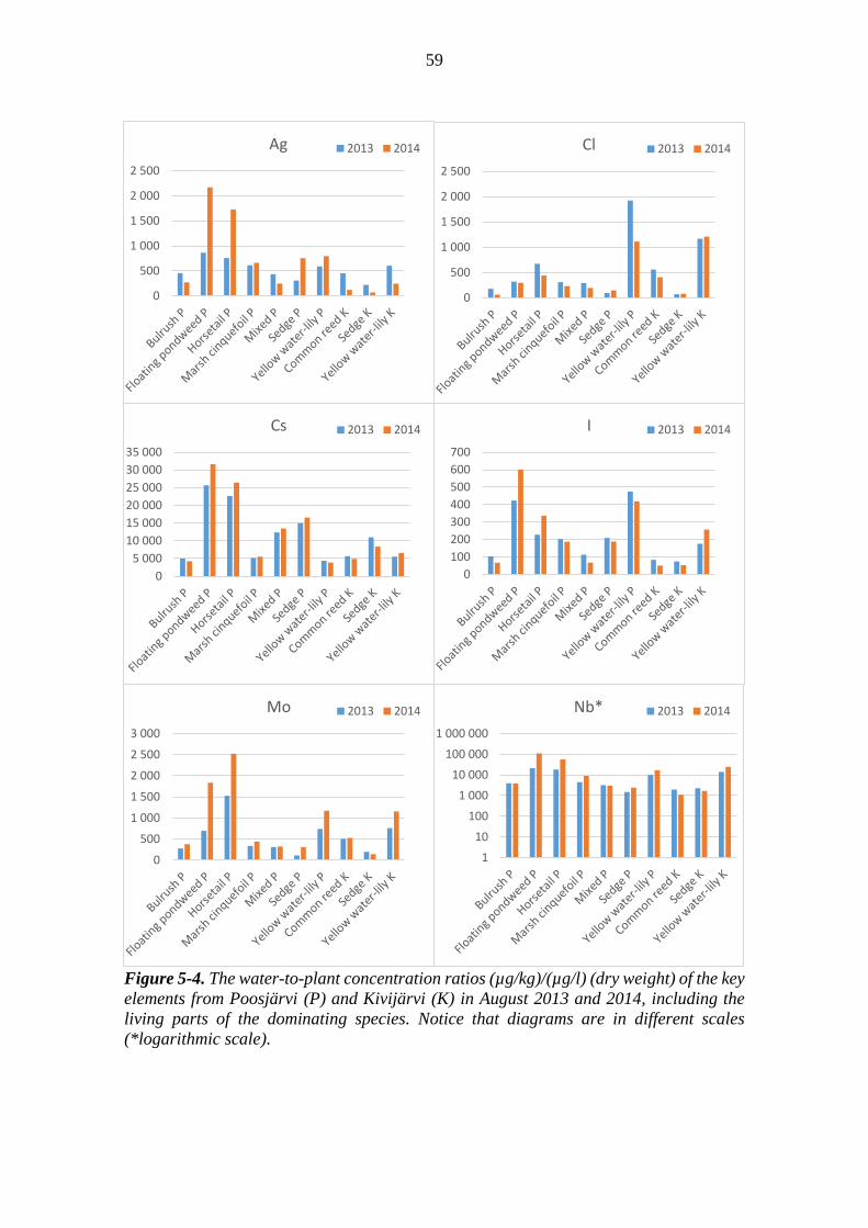
59
0
500
1 000
1 500
2 000
2 500
Ag 2013 2014
0
5 000
10 000
15 000
20 000
25 000
30 000
35 000
Cs 2013 2014
0
100
200
300
400
500
600
700
I 2013 2014
0
500
1 000
1 500
2 000
2 500
3 000
Mo 2013 2014
1
10
100
1 000
10 000
100 000
1 000 000
Nb* 2013 2014
Figure 5-4. The water-to-plant concentration ratios (µg/kg)/(µg/l) (dry weight) of the key
elements from Poosjärvi (P) and Kivijärvi (K) in August 2013 and 2014, including the
living parts of the dominating species. Notice that diagrams are in different scales
(*logarithmic scale).
0
500
1 000
1 500
2 000
2 500
Cl 2013 2014

60
0
1 000
2 000
3 000
4 000
5 000
6 000
Ni 2013 2014
0
20 000
40 000
60 000
80 000
100 000
Pb 2013 2014
1
10
100
1 000
10 000
100 000
Pd* 2013 2014
0
200
400
600
800
1 000
1 200
1 400
Se 2013 2014
0
5 000
10 000
15 000
20 000
Sn 2013 2014
0500
1 0001 5002 0002 5003 0003 5004 000
Sr 2013 2014
Figure 5-4 (cont’d). The water-to-plant concentration ratios (µg/kg)/(µg/l) (dry weight)
of the key elements from Poosjärvi in August 2013 and 2014, including the living parts of
the dominating species. Notice that diagrams are in different scales (*logarithmic scale).
61
5.3 Discussion
The growth of the aquatic vegetation in lake ecosystem starts in spring after ice cover
has melted. In Lakes Poosjärvi and Kivijärvi the vegetation samples were taken in May,
August and October in 2013 and 2014. Lakes Poosjärvi and Kivijärvi are rather shallow
and the vegetation is abundant and dense in both lakes. The biomasses of living fractions
were naturally lowest in May, which represents the beginning of the growing season. The
highest biomasses were observed in August, when the growing season is intensive. After
that the plants begin to fade and the biomasses diminish and the proportion of dead part
of the biomass (litter) increases.
Aquatic macrophytes are known to represent an immense potential for uptake of variety
of contaminants, including heavy metals, inorganic/organic pollutants, radioactive
substances and explosives (Bhupinder et al. 2009). The concentarations of the elements
and the water-to-plant concentration rates vary considerably by species, sampling plot
and sampling date. Concentrations of Cl, Se, Ni and I seem to be highest in every species
in August. Especially water-lily has high concentration and therefore also high
concentration ratio of Cl. The annual variation of element concentrations in plants is low,
so the variation of concentration ratios between the two years is mainly due to annual
variation of element concentrations in water samples. The annual variation in
concentration ratios of Pd is exceptionally wide in every sampling plot in both lakes. It
might be due to the variation of LOQ in different analyses. In general the water-to-plant
concentration ratios are lower in Lake Kivijärvi than in Lake Poosjärvi, which can in
some cases partly be explained by the slightly higher element concentrations in water
samples from Lake Kivijärvi than in water samples from Lake Poosjärvi.

62
63
6 PLANKTON SAMPLES FROM THE LAKES
In this chapter, the results of phytoplankton and zooplankton studies in Lakes Kivijärvi
and Poosjärvi in 2013 and 2014 are presented. Studies were conducted in order to analyse
element concentrations and to calculate water-to-plankton-concentration ratios. In
addition, phytoplankton and zooplankton biomass and species composition were studied
in both lakes and years. There are no previous studies by Posiva on phytoplankton or
zooplankton in the reference lakes.
6.1 Methods
6.1.1 Elements analysis
Phytoplankton and zooplankton samples from Lake Kivijärvi (TMA73-SP7) and Lake
Poosjärvi (TMA71-SP8) were collected from one sampling point in autumn 2013 and
summer 2014. Sampling points are presented in Figure 2-3. Samples for element analyses
were pumped through a plankton net of different mesh sizes and from different depths
according to the Table 6-1. Pumping time and depth varied between samples, lakes and
nets. Samples were collected by Water and Environment Research of South-West Finland
Ltd. The samples were stored in a freezer before sending to the laboratory for the dry
substance and element analyses.
Element concentrations were analysed by ALS Scandinavia AB (Sweden). The whole
sample amount delivered were sieved/filtrated on 50 µm or 100 µm in laboratory (see
Table 6-1), using acid washed filtering cloth. The samples were left to drain on the sieve
as long as water was drained out, no kind of vacuum pump were used. The whole or an
aliquote of the fresh plankton sample were freeze dried before analysis, unit for reporting
µg/kg DS (freeze dried) were used. Total element analysis was carried out after digestion
with HNO3/HF(trace). Analysis was carried out for about 70 elements by ICP-SFMS with
methane addition to achieve the best possible LOQs for Ag and Pd, separate analytical
run for Br, Cl and I. All elements were analysed quantitative. Results were supplied in
the form of Excel reports including both the limits of quantification (<LOQ) and the
measured concentrations, even when the latter are <LOQ. Carbon and nitrogen
concentrations were not analysed due to the lack of the phyto- and zooplankton material.
To calculate water-to-phytoplankton and water-to-zooplankton concentration ratios, three
alternative calculation methods and data were used. First, in separate lakes and years, the
water results of plankton sampling points (SP7 in Kivijärvi and SP8 in Poosjärvi) of the
same sampling date as for plankton are used. Second, for both lakes and years, all water
results of all water sampling points are used in calculations in order to use as much data
as possible and to reduce variation. Third, water results only from August and September
in 2013 and 2014 are used in calculations, and all water sampling points are included.
64
6.1.2 Species and biomass analysis
Phytoplankton and zooplankton samples from Lake Kivijärvi (TMA73-SP7) and Lake
Poosjärvi (TMA71-SP8) were collected from one sampling point in autumn 2013, spring
2014, summer 2014, and autumn 2014 (see Table 6-2). Samples were collected and later
analysed by Water and Environment Research of South-West Finland Ltd.
Phytoplankton samples were collected from the euphotic zone as composite samples by
a Limnos sampler. Sampling water was collected into a bucket and mixed thoroughly,
and the sample was placed into a 200 ml glass bottle with acid Lugol’s solution. The
samples were stored in a freezer before the analyses of phytoplankton biomass and species
composition. Phytoplankton cells were counted with a Leica DM13000 B microscope by
a quantitative method based on SFS-EN 15204 standard (CEN 2006). The phytoplankton
were identified and counted from different sample sizes (3 ml, 5 ml or 10 ml) on account
of differences in the densities of cells in the samples. In identification, 788x, 500x, 250x
and 125x magnification were used, with the magnification factor depending on the size
of species. Cell counts were converted to volumes in line with specific conversion
coefficients. The biomasses were reported as wet weight (µg/l).
Zooplankton samples were collected from the euphotic zone as composite samples by a
Limnos sampler. Two subsamples from each depth (0, 0.5, 1.0, 1.5, 2.0, 2.4, see Table 6-
2) were sieved through a plankton net of mesh size 25 µm, after which the combined
sample was poured into a plastic bottle. Ethanol (ETAX-B, 90%) was used to wash the
biomass from the net to the sampling bottle. Additional ethanol was placed in the
sampling bottle to ensure preservation of the sample before analyses of zooplankton
biomasses and species composition. In this study, both the mesozooplankton (0.2–2 mm,
big rotifers, water fleas, cyclopoids and calanoids) and microzooplankton (small rotifers
of size 20–200 µm) were analysed.
In the laboratory, samples were filtered with a 25 µm (rotifers and crustacea) and 50 µm
(crustacea) filter and sieved or diluted with tap water. The volume of the sample was
measured in graduated glassware/plastic vessels. Sub-samples (1/10 of the full volume)
were taken from each sample for identifying and counting crustacean and rotifers
specimens with the count ceilings being each 200 individuals overall and 50 of nauplius
stage. The sub-samples were further filtered with a 25 µm filter and sieved or diluted with
tap water. If the threshold of 200 individuals was not reached, counting was conducted
for additional sub-samples, with a dilution factor of 1/100. Both the samples and the sub-
samples were mixed extensively, to enable all organisms to become distributed randomly
throughout the sample volume. A few drops of a detergent were added, to reduce the
surface tension of the sample and allow the cladocerans to settle at the bottom of a cuvette.
Zooplankton species were identified and counted with an inverted microscope using 40×,
100×, and 200× magnification factors, across the entire surface area of the cuvette. All
the individuals of crustacea were also measured. The taxonomic groups of crustaceans
considered included species, genera, families, sex, and the various development stages of
copepods. Biomasses were calculated by using the special zooplankton program and
expressed as mg C/m3. Further, the number of individuals was also calculated in 2014 but
not in 2013.

65
Table 6-1. Phytoplankton and zooplankton samples from Lake Kivijärvi (TMA73-SP7)
and Lake Poosjärvi (TMA71-SP8) in autumn 2013 and summer 2014 for element
analyses.
Sample Sampling
point
Sample (pumping)
number Pumping time / mesh size
Pumping depth (m)
Sampling date
Filter size used
in ALS
Autumn 2013
Zooplankton Kivijärvi SP7 I 1 h / 100 µm, 1 h / 50 µm 1.0–1.5 18.9.2013 50 µm
Phytoplankton Kivijärvi SP7 II 2 h / 50 µm 0-0.5 18.9.2013 50 µm
Phytoplankton Kivijärvi SP7 II 2 h / 50 µm 0-0.5 18.9.2013 100 µm
Zooplankton Poosjärvi SP8 I 1 h / 50 μm 1.0 19.9.2013 50 µm
Zooplankton Poosjärvi SP8 I 1 h /100 μm 1.0 19.9.2013 100 µm
Phytoplankton Poosjärvi SP8 II 2 h / 50 μm and 100 μm 0.5 19.9.2013 50 µm
Summer 2014
Zooplankton Kivijärvi SP7 I 1 h / 50 µm, 1 h / 100 µm 1.0–1.5 13.8.2014 50 µm
Phytoplankton Kivijärvi SP7 II 2 h / 50 µm 0-0.5 13.8.2014 50 µm
Zooplankton Poosjärvi SP8 I 1 h / 50 µm, 1 h / 100 µm 1.0 14.8.2014 50 µm
Phytoplankton Poosjärvi SP8 II 2 h / 100 µm 0.5 14.8.2014 50 µm
Table 6-2. Phytoplankton and zooplankton samples from Lake Kivijärvi (TMA73-SP7)
and Lake Poosjärvi (TMA71-SP8) in 2013 and 2014 for species and biomass analyses.
Kivijärvi SP7 Poosjärvi SP8
Time of year Sampling date Sampling depth (m) Sampling date Sampling depth (m)
Phytoplankton
Autumn 2013 Spring 2014
Summer 2014 Autumn 2014
18.9.2013 21.5.2014 13.8.2014 7.10.2014
0–2.0 0–2.0 0–2.0 0–2.0
19.9.2013 21.5.2014 14.8.2014 7.10.2014
0–1.0 0–1.0 0–1.2 0–1.3
Zooplankton
Autumn 2013 Spring 2014
Summer 2014 Autumn 2014
18.9.2013 21.5.2014 13.8.2014 7.10.2014
0–2.0 0–2.0 0–2.4 0–2.0
19.9.2013 21.5.2014 14.8.2014 7.10.2014
0–1.0 0–1.0 0–1.2 0–1.3

66
6.2 Results
6.2.1 Elements
The mean element concentrations of the key elements for phytoplankton and zooplankton
samples are presented in Tables 6-3 and 6-4, respectively. For years, the means of
different mesh sizes are shown, but the samples are from the same sampling dates. For all
the elements, calculated data are presented in Appendix E in Table E-2. Unreliable
laboratory results such as values below the LOQ (limits of quantification) and values over
the LOQ but marked with “<” were not used in calculations. The original results of the
element concentrations are presented in Appendix E in Table E-1.
Due to the low biomass of the phytoplankton and zooplankton samples, nitrogen and
carbon concentrations were not obtained as analysing the element concentrations was set
as the priority.
Water-to-phytoplankton and water-to-zooplankton concentration ratios of the key
elements are presented in Tables 6-5 and 6-6, respectively. Further, concentration ratios
of all the elements are presented in Appendix E in Table E-3.
Table 6-3. Element concentrations of key elements (μg/kg in dry weight) in phytoplankton
samples in Lakes Kivijärvi and Poosjärvi in 2013 and 2014 and in both lakes. Arithmetic
means of different mesh sizes are presented separately for both lakes and years. In
addition, statistics (AM, STD, Min., Max., n) for both lakes and years are presented.
Kivijärvi SP7 Poosjärvi SP8 Both lakes
year 2013 2014 2013 2014 2013 and 2014
Element AM AM AM AM AM STD Min. Max. n
Ag 88.6 86.2 126 47.9 87.5 27.6 47.9 126 5
Cl 170000 183000 150000 78900 151000 44300 78900 191000 5
Cs 3030 1720 1370 238 1880 1180 238 3080 5
I 14700 20800 13600 24200 17600 4710 13600 24200 5
Mo 1390 748 1270 362 1030 460 362 1390 5
Nb 4350 2950 2170 577 2880 1600 577 4610 5
Ni 38000 17100 28600 5680 25500 14000 5680 38600 5
Pb 22000 16500 25100 6540 18400 7330 6540 25100 5
Pd N.A. 51.5 N.A. 16.6 34.1 24.7 16.6 51.5 2
Se 944 1360 935 1230 1080 199 935 1360 5
Sn 1350 1030 925 279 988 440 279 1350 5
Sr 77800 80700 48000 52200 67300 15900 48000 80700 5

67
Table 6-4. Element concentrations of key elements (μg/kg in dry weight) in zooplankton
samples in Lakes Kivijärvi and Poosjärvi in 2013 and 2014 and in both lakes. Arithmetic
means of different mesh sizes are presented separately for both lakes and years. In
addition, statistics (AM, STD, Min., Max., n) for both lakes and years are presented.
Kivijärvi SP7 Poosjärvi SP8 Both lakes
year 2013 2014 2013 2014 2013 and 2014
Element AM AM AM AM AM STD Min. Max. n
Ag 80.9 49.3 142 110 97.6 44.5 29.8 160 7
Cl 181000 180000 195000 192000 188000 27600 154000 227000 7
Cs 2740 679 1500 1080 1320 804 172 2740 7
I 14800 34000 13700 19200 21200 10200 13100 42000 7
Mo 1340 487 1940 964 1160 771 332 2680 7
Nb 4050 1120 2370 2080 2170 1180 345 4050 7
Ni 37100 9390 35200 24200 25000 13500 5550 42200 7
Pb 21500 29800 25900 15300 23300 7950 10300 36000 7
Pd N.A 33.8 N.A. 68.3 45.3 23.1 22.1 68.3 3
Se 1060 1470 917 1390 1230 358 845 1820 7
Sn 1200 646 1120 945 946 368 350 1370 7
Sr 73900 50600 50300 54600 55000 14700 32800 73900 7
Table 6-5. Water-to-biota concentration ratios ((µg/kg)/(µg/l) in dry) of the key elements,
for the phytoplankton communities sampled from the Lakes Poosjärvi and Kivijärvi in
2013 and 2014.
A: In separate lakes and years, the water results only from plankton sample points (SP7
in Kivijärvi and SP8 in Poosjärvi) of same sampling date are used. For both lakes and
years 2013 and 2014, all results of all water sampling points are used in calculations.
Kivijärvi Poosjärvi Both lakes
Key element 2013 2014 2013 2014 2013 and 2014
Ag 6870 N.A. 10100 N.A. 3140
Cl 43 49 49 18 52
Cs 352000 171000 148000 17900 207000
I 3680 4050 3610 3630 3890
Mo 14000 3880 11900 1650 8600
Nb 1010000 2090000 615000 412000 787000
Ni 26400 12500 18700 3140 17000
Pb 411000 N.A. 428000 568000 523000
Pd N.A. N.A. N.A. 3170 16500
Se N.A. 19300 12300 N.A. 5930
Sn 43400 N.A. 131000 N.A. 59900
Sr 3780 3010 2290 1710 2710
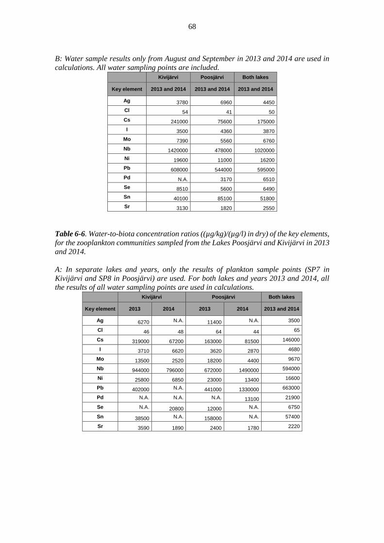
68
B: Water sample results only from August and September in 2013 and 2014 are used in
calculations. All water sampling points are included.
Kivijärvi Poosjärvi Both lakes
Key element 2013 and 2014 2013 and 2014 2013 and 2014
Ag 3780 6960 4450
Cl 54 41 50
Cs 241000 75600 175000
I 3500 4360 3870
Mo 7390 5560 6760
Nb 1420000 478000 1020000
Ni 19600 11000 16200
Pb 608000 544000 595000
Pd N.A. 3170 6510
Se 8510 5600 6490
Sn 40100 85100 51800
Sr 3130 1820 2550
Table 6-6. Water-to-biota concentration ratios ((µg/kg)/(µg/l) in dry) of the key elements,
for the zooplankton communities sampled from the Lakes Poosjärvi and Kivijärvi in 2013
and 2014.
A: In separate lakes and years, only the results of plankton sample points (SP7 in
Kivijärvi and SP8 in Poosjärvi) are used. For both lakes and years 2013 and 2014, all
the results of all water sampling points are used in calculations.
Kivijärvi Poosjärvi Both lakes
Key element 2013 2014 2013 2014 2013 and 2014
Ag 6270 N.A. 11400 N.A. 3500
Cl 46 48 64 44 65
Cs 319000 67200 163000 81500 146000
I 3710 6620 3620 2870 4680
Mo 13500 2520 18200 4400 9670
Nb 944000 796000 672000 1490000 594000
Ni 25800 6850 23000 13400 16600
Pb 402000 N.A. 441000 1330000 663000
Pd N.A. N.A. N.A. 13100 21900
Se N.A. 20800 12000 N.A. 6750
Sn 38500 N.A. 158000 N.A. 57400
Sr 3590 1890 2400 1780 2220
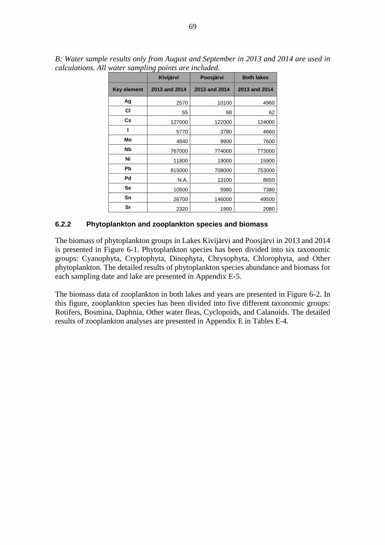
69
B: Water sample results only from August and September in 2013 and 2014 are used in
calculations. All water sampling points are included.
Kivijärvi Poosjärvi Both lakes
Key element 2013 and 2014 2013 and 2014 2013 and 2014
Ag 2570 10100 4960
Cl 55 68 62
Cs 127000 122000 124000
I 5770 3780 4660
Mo 4840 9900 7600
Nb 767000 774000 773000
Ni 11800 19000 15900
Pb 815000 708000 753000
Pd N.A. 13100 8650
Se 10500 5980 7380
Sn 26700 146000 49500
Sr 2320 1900 2080
6.2.2 Phytoplankton and zooplankton species and biomass
The biomass of phytoplankton groups in Lakes Kivijärvi and Poosjärvi in 2013 and 2014
is presented in Figure 6-1. Phytoplankton species has been divided into six taxonomic
groups: Cyanophyta, Cryptophyta, Dinophyta, Chrysophyta, Chlorophyta, and Other
phytoplankton. The detailed results of phytoplankton species abundance and biomass for
each sampling date and lake are presented in Appendix E-5.
The biomass data of zooplankton in both lakes and years are presented in Figure 6-2. In
this figure, zooplankton species has been divided into five different taxonomic groups:
Rotifers, Bosmina, Daphnia, Other water fleas, Cyclopoids, and Calanoids. The detailed
results of zooplankton analyses are presented in Appendix E in Tables E-4.
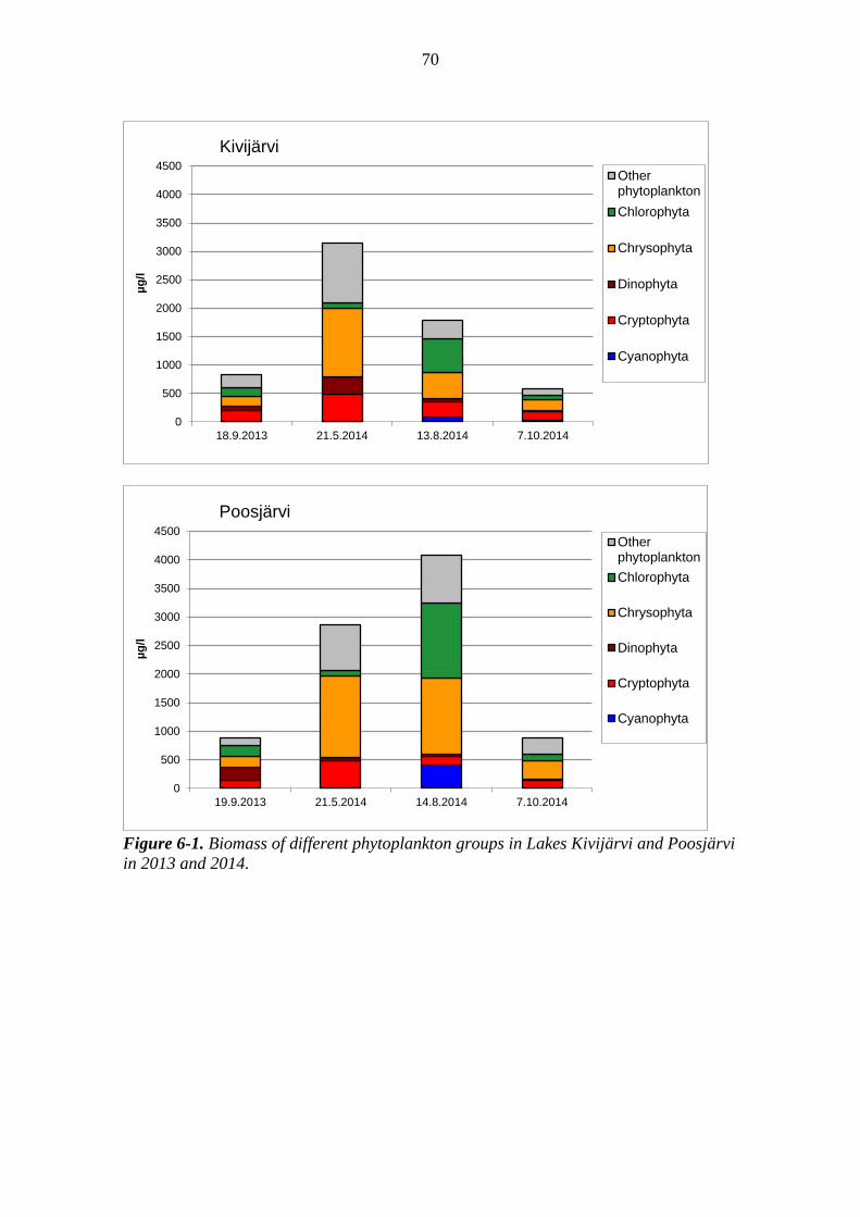
70
Figure 6-1. Biomass of different phytoplankton groups in Lakes Kivijärvi and Poosjärvi
in 2013 and 2014.
0
500
1000
1500
2000
2500
3000
3500
4000
4500
18.9.2013 21.5.2014 13.8.2014 7.10.2014
µg
/lKivijärvi
Otherphytoplankton
Chlorophyta
Chrysophyta
Dinophyta
Cryptophyta
Cyanophyta
0
500
1000
1500
2000
2500
3000
3500
4000
4500
19.9.2013 21.5.2014 14.8.2014 7.10.2014
µg
/l
Poosjärvi
Otherphytoplankton
Chlorophyta
Chrysophyta
Dinophyta
Cryptophyta
Cyanophyta

71
Figure 6-2. Biomass of different zooplankton groups in Lakes Kivijärvi and Poosjärvi
in 2013 and 2014.
0
10
20
30
40
50
60
70
18.9.2013 21.5.2014 13.8.2014 7.10.2014
mg
C/m
3
Kivijärvi
Calanoids
Cyclopoids
Other waterfleas
Daphnia
Bosmina
Rotifers
0
10
20
30
40
50
60
70
19.9.2013 21.5.2014 14.8.2014 7.10.2014
mg
C/m
3
Poosjärvi
Calanoids
Cyclopoids
Other waterfleasDaphnia
Bosmina
Rotifers
72
6.3 Discussion
6.3.1 Element concentrations and concentration ratios in phytoplankton and zooplankton
The concentrations of the key elements in phytoplankton and zooplankton were of same
magnitude in both lakes and years and as means of both lakes and years (see Tables 6-3
and 6-4). In some key elements (Cs, Mo, Nb, Ni, Sn), concentrations on both
phytoplankton and zooplankton were higher in 2013 compared to 2014 in both lakes. For
other elements, there were no clear differences between the study years. In addition, for
some key elements (Cl, Cs, Nb, Ni, Sn, Sr), the concentrations in phytoplankton were
higher in Lake Kivijärvi compared to Lake Poosjärvi in both years. For zooplankton, no
similar lake-specific differences were observed, and some concentrations (Ag, Mo)
tended to be even higher in Lake Poosjärvi than in Lake Kivijärvi. There are no earlier
results on element concentrations in phytoplankton or zooplankton in the reference lakes.
Water-to-phytoplankton and water-to-zooplankton concentration ratios were calculated
in many different combinations by using water analyses results from different sampling
times or sampling points (Tables 6-5 and 6-6). As a conclusion, there were no major
differences between concentration ratios concerning different ways of calculations. The
concentration ratios of some key elements (Cs, Mo, Ni, Sr) were higher in 2013 compared
to 2014 in phyto- and zooplankton in both lakes. Furthermore, the water-to-phytoplankton
concentration ratios for Cs, Mo, Nb, Ni and Sr were higher in Lake Kivijärvi compared
to Lake Poosjärvi in both years. However, the water-to-zooplankton concentration ratios
for Ag, Mo and Sn tended to be higher in Lake Poosjärvi compared to Lake Kivijärvi in
both years. Thus, some spatial and temporal variation in concentrations as well as in
concentration ratios concerning plankton was observed.
6.3.2 Phytoplankton species and biomass
In Lake Kivijärvi, the total phytoplankton biomass as mean of all sampling dates was
1 580 µg/l, and it ranged from 586 µg/l in October 2014 to 3 150 µg/l in May 2014. The
mean total phytoplankton biomass in Lake Poosjärvi was 2 174 µg/l ranging from
875 µg/l in October 2014 to 4078 µg/l in August 2014. Thus, the mean total biomass in
Lake Poosjärvi was higher than in Lake Kivijärvi mainly due to the high biomass in Lake
Poosjärvi in August 2014. In both lakes, phytoplankton biomasses in September 2013 and
in October 2014 were lower compared to the other sampling dates. Lakes Kivijärvi and
Poosjärvi are typed as “shallow lakes rich in humus (MRh)” in Water Framework
Directive. According to the mean total biomass of phytoplankton in June–August, the
ecological state of Lake Kivijärvi was excellent and that of Lake Poosjärvi good.
There were no major differences in phytoplankton community structure between different
sampling dates or lakes. Chysophyta dominated the phytoplankton in all the other samples
except that of August 2014 in Lake Kivijärvi and September 2013 in Lake Poosjärvi,
accounting for 22–49 % of the total biomass. In May 2014, the dominating species of
Chysophyta was Uroglena sp. in both lakes. In August 2014, the proportion of
Chlorophyta was high (33 %) in both lakes, with the class Chlorophyceae dominating,
whereas in other samples its share was clearly lower (3–21 %). In September 2013,
Dinophyta was the dominating group in Lake Poosjärvi with a share of 25 %, but

73
otherwise the biomasses of Dinophyta were low. Cryptophyta accounted for 4–27 % of
the phytoplankton biomass. The proportion of “Other phytoplankton” (i.e. monads and
flagellates) was relatively high in all samples and accounted for 16– 33 % of the total
biomass. In Lake Poosjärvi, the biomass of Cyanophyta was slightly elevated in August
2014, but otherwise the proportions of Cyanophyta remained low (< 5 %).
6.3.3 Zooplankton species and biomass
In Lake Kivijärvi, the total zooplankton biomass ranged from 4.0 mg C/m3 in October
2014 to 46 mg C/m3 in August 2014. In Lake Poosjärvi, the total zooplankton biomass
ranged from 17 mg C/m3 to 69 mg C/m3; biomass was lowest in October 2014 and highest
in May 2014. Like in phytoplankton, zooplankton biomasses in September 2013 and in
October 2014 were lower compared to the other sampling dates. In each sampling date,
the biomasses of Lake Poosjärvi were higher compared to that of Lake Kivijärvi. In May
2014, the zooplankton biomass in Lake Poosjärvi was the highest of all the samples.
Overall, the biomass levels of both lakes were rather low. However, in this study, the
biomass maximum may already have been over in mid-August, because the zooplankton
biomasses are usually at their highest earlier in summer.
In both lakes, rotifers dominated the zooplankton biomasses in September 2013, and the
most common species was Polyarthra remata typical for late summer and autumn. In
Lake Kivijärvi, rotifers dominated also in May 2014, but the dominating species was
Keratella cochlearis v. hispida. Rotifers are typically more common in spring than later
in summer. In Lake Poosjärvi in May 2014, the biomass of rotifers was at the same level
as in Lake Kivijärvi, but the dominating group was, however, Bosmina water fleas with
Bosmina coregoni accounting for the largest part of the Bosmina biomass. In August
2014, Cyclopoids and especially Thermocyclops oithonoides females and copepodites
formed the largest part of the zooplankton biomass in Lake Kivijärvi. In Lake Poosjärvi,
the dominating group in August 2014 was “other water fleas” (e.g. Diaphanosoma
brachyurum). In October 2014, zooplankton biomasses were low in both lakes.

74
75
7 MACROBENTHOS
In this chapter, the results of the macrobenthos studies in Lakes Kivijärvi and Poosjärvi
in 2013 and 2014 are presented. The aim of the study was to collect macrobenthos and
mussel samples for the element analysis. In addition, macrobenthos samples were
collected for determination of species composition, biomass, and abundance. Mussel
samples were also collected for biomass analyses and dimension measures.
In the previous study by Posiva in 2010, macrobenthos samples were collected from Lake
Koskeljärvi and from Lake Lutanjärvi (Kangasniemi et al. 2014). In 2011–2012,
macrobenthos studies were not conducted in reference lakes (Kangasniemi et al. 2016).
7.1 Methods
7.1.1 Mussels for element analysis and size measurements
The mussel samples were collected from Lakes Poosjärvi and Kivijärvi in autumns 2013
and 2014 for element analysis. Mussels were collected by diving by Monivesi Oy from
three sampling points in both lakes. Sampling sites and dates are presented in Figure 2-3
and in Table 7-1. Both living and dead mussels were collected.
In 2014, after collecting the mussels, the sediment was carefully brushed away from the
mussels in lake shore. In 2013 similar brushing was not done. Mussels were carefully
opened by a knife and shaken to remove extra water. The samples were put into the plastic
bags with identifying data, and stored in a cool place before transporting to a freezer.
The samples of year 2013 and year 2014 were processed in November 2014 (24–26th) and
in October 2014 (24th and 28–29th), respectively. Processing took place in the laboratory
and by personnel of EnviroCase Ltd. Mussels were taken out of the freezer a day before
the treatment. During defrosting extra water was drilled away from the plastic bags
through a small hole. With samples of year 2013, all the instruments were rinsed with
distilled Milli-Q water, whereas with samples of year 2014, lake water was used in
rinsing. Individuals of Anadonta sp. and Unio sp. were treated separately with exception
of sampling point SP9 in Lake Kivijärvi in 2014. Mussels of sampling point SP9 in 2014
were the first ones to be treated, and they were not handled as separate species. Thus,
there is a mixed mussel sample for SP9 in Lake Kivijärvi in 2014.
All the mussels collected were not used for elements analysis due to the high number of
individuals. However, the length of all the mussels was measured and the fresh biomass
was weighted with an analytical balance. Then, individual mussels were sorted based on
their fresh weight. In order to ensure the adequate amount of the sample (10 g fresh) some
samples were combined before sending them to laboratory. The individuals chosen for
elements analyses represented different size categories. Size categories and number of
individuals chosen for subsamples from each category were:
fresh weight >20 g: one individual chosen for subsample;
fresh weight 10-20 g: two individuals chosen for subsample;
fresh weight <10 g: three individuals chosen for subsample;
fresh weight <5 g: four individuals chosen for subsample (not used in 2014)

76
Altogether five subsamples per sampling point and per species were gathered from both
lakes and years if possible. All the mussels used for elements analyses were photographed
(Figure 7-1). Mussels were opened and meat was separated from the shell with a knife.
Shell and meat were weighted separately. Every subsample was packed to the plastic bag
and put to a freezer before sending to the laboratory. Subsamples were further combined
before sending to the laboratory so that 1–2 analyses of meat and shell per sampling point
and per species for both lakes and years were conducted.
The element concentrations and carbon and nitrogen concentrations of mussel samples
were analysed by ALS Scandinavia AB (Sweden). For dry matter analysis wet samples
or samples dried at 50°C were homogenised before digestion and analysis. A separate DS
105°C was carried out on the wet and 50°C dried samples. Final results were recalculated
and reported in unit µg/kg DS105°C. Total element analysis was carried out after
digestion of wet or 50°C dried and homogenised samples. Samples were digested in
microwave oven with HNO3 and HF (trace). After dilution, analysis was carried out for
about 70 elements by ICP-SFMS with methane addition to achieve the best possible
LOQs for Ag and Pd, separate analytical run (alkaline) for Br, Cl and I. All elements were
analyzed quantitatively. Results reports include both the limits of quantification (<LOQ)
and the measured concentrations, even when the latter are <LOQ.
7.1.2 Macrobenthos for elements analysis
The macrobenthos samples for element analysis were collected by a so-called mammoth
pump invented by Ari Ruuskanen/Monivesi Oy. The principle of a mammoth pump is
based on suction created by compressed air (see Kirkkala et al. 2017, Figure 7-1).
Cylinder shaped sampler is placed on the bottom of the sediment, and compressed air is
lead into the tube running from bottom to surface through a sampler. Water, bottom
sediment, and macrobenthos are pulled up by rising air bubles in the tube. In the top of
the tube, macrobenthos and coarse bottom material are sieved through a net (mesh size
0.5-mm) and gathered into a collector.
Samples were collected from Lakes Poosjärvi and Kivijärvi in autumns 2013 and 2014
by Monivesi Oy. Samples were collected from three sampling points in both lakes
simultaneously as mussel samples; sampling points and dates are presented in Table 7-1.
The number of sub-samples (i.e. the number of short suctions of the pump) was 15–20 in
each sampling point. Sampling depth was c.a. 5 cm and the water depth in sampling points
was 1.2 m. The samples were placed in clean plastic containers filled with water from the
same sampling point. The samples were stored in a freezer before the pre-treatment.
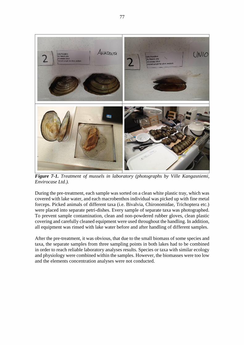
77
Figure 7-1. Treatment of mussels in laboratory (photographs by Ville Kangasniemi,
Envirocase Ltd.).
During the pre-treatment, each sample was sorted on a clean white plastic tray, which was
covered with lake water, and each macrobenthos individual was picked up with fine metal
forceps. Picked animals of different taxa (i.e. Bivalvia, Chironomidae, Trichoptera etc.)
were placed into separate petri-dishes. Every sample of separate taxa was photographed.
To prevent sample contamination, clean and non-powdered rubber gloves, clean plastic
covering and carefully cleaned equipment were used throughout the handling. In addition,
all equipment was rinsed with lake water before and after handling of different samples.
After the pre-treatment, it was obvious, that due to the small biomass of some species and
taxa, the separate samples from three sampling points in both lakes had to be combined
in order to reach reliable laboratory analyses results. Species or taxa with similar ecology
and physiology were combined within the samples. However, the biomasses were too low
and the elements concentration analyses were not conducted.
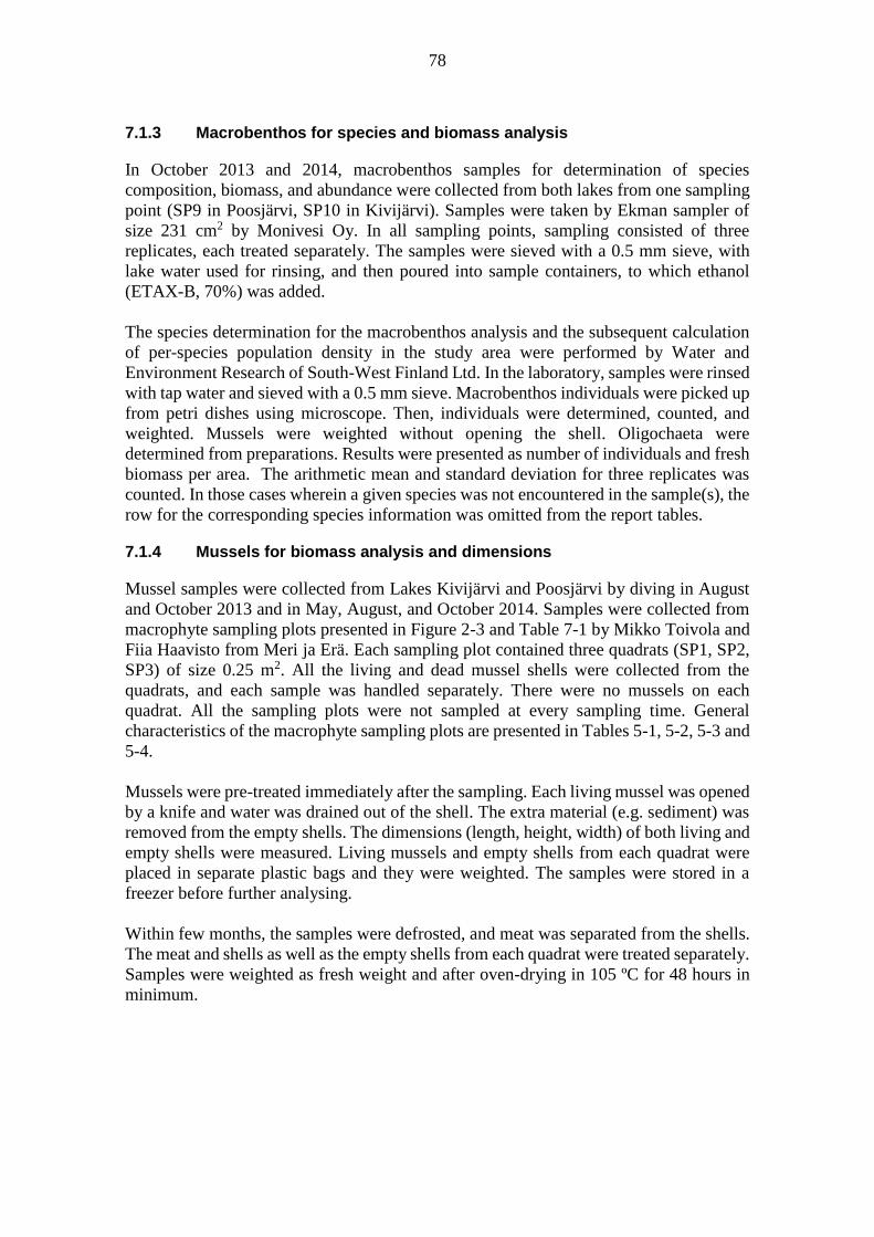
78
7.1.3 Macrobenthos for species and biomass analysis
In October 2013 and 2014, macrobenthos samples for determination of species
composition, biomass, and abundance were collected from both lakes from one sampling
point (SP9 in Poosjärvi, SP10 in Kivijärvi). Samples were taken by Ekman sampler of
size 231 cm2 by Monivesi Oy. In all sampling points, sampling consisted of three
replicates, each treated separately. The samples were sieved with a 0.5 mm sieve, with
lake water used for rinsing, and then poured into sample containers, to which ethanol
(ETAX-B, 70%) was added.
The species determination for the macrobenthos analysis and the subsequent calculation
of per-species population density in the study area were performed by Water and
Environment Research of South-West Finland Ltd. In the laboratory, samples were rinsed
with tap water and sieved with a 0.5 mm sieve. Macrobenthos individuals were picked up
from petri dishes using microscope. Then, individuals were determined, counted, and
weighted. Mussels were weighted without opening the shell. Oligochaeta were
determined from preparations. Results were presented as number of individuals and fresh
biomass per area. The arithmetic mean and standard deviation for three replicates was
counted. In those cases wherein a given species was not encountered in the sample(s), the
row for the corresponding species information was omitted from the report tables.
7.1.4 Mussels for biomass analysis and dimensions
Mussel samples were collected from Lakes Kivijärvi and Poosjärvi by diving in August
and October 2013 and in May, August, and October 2014. Samples were collected from
macrophyte sampling plots presented in Figure 2-3 and Table 7-1 by Mikko Toivola and
Fiia Haavisto from Meri ja Erä. Each sampling plot contained three quadrats (SP1, SP2,
SP3) of size 0.25 m2. All the living and dead mussel shells were collected from the
quadrats, and each sample was handled separately. There were no mussels on each
quadrat. All the sampling plots were not sampled at every sampling time. General
characteristics of the macrophyte sampling plots are presented in Tables 5-1, 5-2, 5-3 and
5-4.
Mussels were pre-treated immediately after the sampling. Each living mussel was opened
by a knife and water was drained out of the shell. The extra material (e.g. sediment) was
removed from the empty shells. The dimensions (length, height, width) of both living and
empty shells were measured. Living mussels and empty shells from each quadrat were
placed in separate plastic bags and they were weighted. The samples were stored in a
freezer before further analysing.
Within few months, the samples were defrosted, and meat was separated from the shells.
The meat and shells as well as the empty shells from each quadrat were treated separately.
Samples were weighted as fresh weight and after oven-drying in 105 ºC for 48 hours in
minimum.

79
Table 7-1. Macrobenthos and mussel samples from Lake Kivijärvi (TMA73) and Lake
Poosjärvi (TMA71) in 2013 and 2014.
Kivijärvi (TMA73) Poosjärvi (TMA71)
Macrobenthos by Mammoth
pump and mussels by
diving
Macrobenthos by Ekman
Mussels by diving for biomass
Macrobenthos by Mammoth
pump and mussels by
diving
Macrobenthos by Ekman
Mussels by diving for biomass
Time of year Sampling date Sampling date
Spring 2013 - - - - - -
Summer 2013 - - 19.-20.8.2013 - - 21.-22.8.2013
Autumn 2013 8.10.2013 8.10.2013 7.-8.10.2013 9.10.2013 9.10.2013 9.-10.10.2013
Spring 2014 - - 12.-13.5.2014 - - 14.-15.5.2014
Summer 2014 - - 11.-12.8.2014 - - 13.-14.8.2014
Autumn 2014 13.10.2014 13.10.2014 13.-14.10.2014 15.10.2014 15.10.2014 15.-16.10.2014
Sampling points
SP11, SP12, SP13
SP10 OA1, OA2,
OA5
(Macrophyte sampling plots)
SP10, SP11, SP12
SP9 OA2, OA3, OA4,
OA7, OA8
(Macrophyte sampling plots)
Table 7-2. General characteristics and species found of the macrobenthos samples
collected by mammoth pump from Lakes Kivijärvi and Poosjärvi in 2014 for elements
analyses. For 2013, data is missing.
Sampling point
Assesment biotope
Water depth (m)
Observed species
Kivijärvi
SP11 soft photic 1.2 Chironomus sp. (including Chironomus plumosus, Orthocladius sp.), Chaoborus sp., Hydrachnidia (including Limnochares aquatica), Trichoptera
SP12 soft photic 1.2 Chironomus sp. (including Chironomus plumosus, Orthocladius sp.), Chaoborus sp., Hydrachnidia (including Limnochares aquatica), Trichoptera
SP13 soft photic 1.2 Chironomus sp. (including Chironomus plumosus, Orthocladius sp.), Chaoborus sp., Hydrachnidia (including Limnochares aquatica), Trichoptera, Asellus aquaticus, Oligochaeta (including Tubifex tubifex and Lumbriculus variegatus), Pisidium sp., Sphaerium corneum, Unio sp., Anadonta sp. (empty shell), Bithynia tentaculata, Odonata sp., Ephemera sp.
Poosjärvi
SP10 soft photic 1.2 Chironomus sp. (including Chironomus plumosus), Chaoborus sp., Hydrachnidia (including Limnochares aquatic and Unionicola sp.), Oligochaeta (including Tubifex tubifex and Lumbriculus variegatus), Pisidium sp., Anadonta sp., Odonata sp.
SP11 soft photic 1.2 Chironomus sp. (including Chironomus plumosus), Hydrachnidia (including Limnochares aquatic and Unionicola sp.), Oligochaeta (including Tubifex tubifex and Lumbriculus variegatus), Pisidium sp., Anadonta sp., Unio sp., Trichoptera sp.
SP12 soft photic 1.2 Chironomus sp. (including Chironomus plumosus), Hydrachnidia (including Limnochares aquatica and Unionicola sp.), Pisidium sp., Unio sp.

80
7.2 Results
7.2.1 Element concentrations, concentration ratios and size measurements
The concentrations of the key elements for mussel samples from Lakes Kivijärvi and
Poosjärvi are presented in Tables 7-3 and 7-4. Only shell and meat data from living
mussels are included. In Table 7-3, arithmetic means of sampling points separately for
both lakes and years as well as for different species are presented. In Table 7-4, statistics
of both lakes and years separately for different species are presented. For all the elements,
calculated data are presented in Appendix F in Table F-1. Unreliable laboratory results
such as values below the LOQ (limits of quantification) and values over the LOQ but
marked with “<” were not used in calculations. The original results of the elements
concentrations of all the mussel samples are presented in Appendix F in Table F-2.
The water-to-mussel concentration ratios of key elements are presented in Tables 7-5 and
7-6. In Table 7-5, concentration ratios for Anadonta sp. and Unio sp. shell and meat have
been calculated separately for both lakes and years. Only living mussels are included. As
water results, the annual means of all water sampling points separately for both lakes are
used in calculation. In Table 7-6, the mean concentration ratios of both lakes and years
are presented. Further, the concentration ratios of all the elements are presented in
Appendix F Table F-3.
Carbon (C) and nitrogen (N) concentrations and dry matter content of mussel shell and
meat samples in Lakes Kivijärvi and Poosjärvi are presented in Tables 7–7 and 7–8. In
Table 7–7, results for Anadonta sp. and Unio sp. shell and meat have been calculated
separately for both lakes and years. Only living mussels are included. In Table 7-8, the
mean values of both lakes and years are presented. The original results of C and N as well
as dry matter content are presented in Appendix F in Table F-4.
The fresh weight, total length and length/weight ratio of living and dead Anadonta sp.
and Unio sp. individuals are presented in Tables 7–9 and 7–10, respectively. Results are
presented as mean for all sampling points and separately for both lakes and years. The
mussels were collected for elements analyses and therefore biomass per area is not
possible to be calculated. In 2014, dead mussels were not found/collected.
.

81
Table 7-3. Element concentrations (μg/kg in dry weight) of key elements in Anadonta sp. and Unio sp. shell and meat samples in Lakes Kivijärvi
and Poosjärvi separately for both lake and year. From Lake Kivijärvi also mixed mussel sample in 2014 (only SP9). Only arithmetic means (AM)
are presented. Only livings mussels included.
Kivijärvi Poosjärvi
2013 2014 2013 2014
Anadonta sp. Unio sp. Anadonta sp. Unio sp. Mussel Anadonta sp. Unio sp. Anadonta sp. Unio sp.
shell meat shell meat shell meat shell meat shell meat shell meat shell meat shell meat shell meat
Element AM AM AM AM AM AM AM AM AM AM AM AM AM AM AM AM AM AM
Ag 9.2 57.5 6.9 65.5 6.52 69.1 8.07 62.6 9.57 41.2 5.58 91.1 4.95 95.9 5.67 151 4.09 46.7
Cl 126000 2770000 99100 1780000 71000 2880000 68500 1460000 67500 2270000 87500 2860000 93100 1660000 64900 2390000 53600 1760000
Cs 33.9 216 18.7 108 13.3 84.9 10.9 73.2 29.8 98.4 3.51 47.4 3.25 40.8 7.97 47.8 1.93 41
I 886 3300 1140 2480 580 3690 1410 2180 586 2650 335 3190 480 1940 330 2620 429 1730
Mo 188 735 206 492 81.7 741 200 476 302 799 41.3 538 69 444 76.6 719 57.9 462
Nb 61.1 359 46.1 134 23.6 115 26.3 73.7 80.3 188 7.74 64.9 8.76 41.7 16.5 51.7 7.82 35.8
Ni 1870 3880 825 2890 990 2660 1100 2150 2810 2870 397 2000 317 1780 818 3530 270 2360
Pb 769 3430 452 1820 343 3230 340 1320 1040 4130 308 3260 187 1240 413 4660 208 1320
Pd 8.05 N.A. 6.89 N.A. 3.12 N.A. 2.87 N.A. 16.8 N.A. N.A. N.A. 1.47 N.A. 3.87 N.A. N.A. N.A.
Se 79.9 1500 62.3 1470 73.4 1600 52.2 1690 43.2 1760 31.1 1340 56.9 1780 77.2 1420 51.3 1460
Sn 29.6 273 23 166 16.9 123 17.2 115 33 130 11 55.6 10.7 44.1 16 115 9.55 90.2
Sr 454000 506000 484000 293000 456000 791000 431000 182000 421000 645000 483000 467000 520000 188000 469000 480000 510000 241000
Table 7-4. Element concentrations (μg/kg in dry weight) of key elements in Anadonta sp. and Unio sp. shell and meat samples in Lakes Kivijärvi
and Poosjärvi in 2013 and 2014. Statistics (AM, STD, Min., Max., n) of both lakes and years presented. Only livings mussels included.
Anadonta sp. Unio sp.
shell meat shell meat
Element AM STD Min. Max. n AM STD Min. Max. n AM STD Min. Max. n AM STD Min. Max. n
Ag 6.73 2.29 3.93 12 13 90.3 81.6 36 345 13 6.1 1.78 3.87 9.1 9 67.4 32.7 44.1 145 9
Cl 89400 29800 51000 149000 11 2740000 438000 1840000 3360000 13 80800 23200 52300 112000 9 1680000 323000 1170000 2130000 9
Cs 14.6 13.3 2.24 44.5 13 98 88.7 34.9 332 13 9.79 8.68 1.63 25.6 9 70.6 33.9 31.1 134 9
I 537 279 234 1250 13 3240 771 2390 5330 13 894 503 286 1540 9 2130 432 1700 3130 9
Mo 95.7 63 28.6 242 13 688 173 439 1030 13 141 105 25.7 296 9 471 89.1 348 657 9
Nb 26.9 23 4.69 71.5 13 145 165 30.4 616 13 24.9 22.4 5.32 69.6 9 78.4 50.4 26.5 186 9
Ni 1020 632 175 2230 13 2990 1280 1600 5530 13 650 520 126 1620 9 2360 871 1410 4440 9
Pb 449 252 137 1080 13 3610 2060 1530 8780 13 314 180 124 662 9 1470 465 977 2550 9
Pd 5.34 2.99 2.78 11.1 7 N.A. - - - 0 4.65 3.78 1.47 11.5 6 N.A. - - - 0
Se 68 25.4 22.9 107 10 1470 222 1050 1740 13 56.4 19.4 38.4 102 9 1590 216 1210 1940 9
Sn 18.3 8.17 9.18 33.9 13 140 113 47.6 384 13 16 7.78 8.06 29.9 9 111 71.5 28.1 272 9
Sr 465000 30700 382000 506000 13 579000 364000 306000 1760000 13 486000 42300 427000 560000 9 234000 115000 115000 505000 9

82
Table 7-5. Water-to-mussel concentration ratios ((µg/kg)/(µg/l) in dry) of the key elements for the Anadonta sp. and Unio sp. shell and meat
calculated separately for Lakes Kivijärvi and Poosjärvi and years 2013 and 2014. From Lake Kivijärvi also mixed mussel sample in 2014. Only
livings mussels included.
Kivijärvi Poosjärvi
2013 2014 2013 2014
Anadonta sp. Unio sp. Anadonta sp. Unio sp. Mussel Anadonta sp. Unio sp. Anadonta sp. Unio sp.
Element shell meat shell meat shell meat shell meat shell meat shell meat shell meat shell meat shell meat
Ag 710 4440 533 5050 131 1390 162 1250 192 826 447 7290 396 7670 489 13000 353 4020
Cl 45.5 999 35.8 645 21.9 887 21.1 450 20.8 701 41.6 1360 44.3 790 21.4 790 17.7 581
Cs 3750 23900 2060 12000 1430 9100 1170 7840 3190 10500 426 5750 395 4960 859 5160 208 4420
I 251 933 322 702 84.9 541 206 319 85.9 388 99.6 948 142 576 85.6 678 111 449
Mo 1690 6630 1860 4430 625 5660 1530 3630 2310 6110 379 4930 633 4070 624 5860 471 3760
Nb 10400 61100 7850 22900 8090 39300 9010 25300 27600 64400 2770 23200 3130 14900 5260 16500 2500 11400
Ni 1210 2520 535 1870 659 1770 732 1430 1870 1910 289 1460 231 1290 533 2300 176 1540
Pb 13100 58600 7730 31000 16400 154000 16300 62900 49500 197000 5670 59900 3430 22700 23300 263000 11700 74700
Pd N.A. N.A. N.A. N.A. 2130 N.A. 1960 N.A. 11500 N.A. N.A. N.A. N.A. N.A. 1680 N.A. N.A. N.A.
Se 173 3240 135 3200 833 18100 593 19200 490 20000 184 7950 336 10500 534 9810 355 10100
Sn 1060 9740 821 5940 1030 7480 1050 7010 2020 7920 1560 7870 1520 6240 1950 14000 1160 11000
Sr 20900 23200 22200 13400 17500 30400 16600 7000 16200 24800 25800 25000 27800 10100 16200 16600 17600 8350

83
Table 7-6. Water-to-mussel concentration ratios ((µg/kg)/(µg/l) in dry) of the key elements for the Anadonta sp. and Unio sp. shell and meat
samples in Lakes Kivijärvi and Poosjärvi in 2013 and 2014. Statistics (GM, GSD, Min., Max., n) of both lakes and years presented. Only livings
mussels included.
Anadonta sp. Unio sp.
shell meat shell meat
Element GM GSD Min. Max. n GM GSD Min. Max. n GM GSD Min. Max. n GM GSD Min. Max. n
Ag 377 2,09 131 710 4 4910 2,59 1390 13000 4 331 1,66 162 533 4 3740 2,17 1250 7670 4
Cl 30,7 1,50 21,4 45,5 4 988 1,26 790 1360 4 27,7 1,54 17,7 44,3 4 604 1,26 450 790 4
Cs 1180 2,50 426 3750 4 8960 2,01 5160 23900 4 666 2,82 208 2060 4 6740 1,58 4420 12000 4
I 116 1,68 84,9 251 4 755 1,31 541 948 4 180 1,59 111 322 4 491 1,40 319 702 4
Mo 707 1,87 379 1690 4 5740 1,13 4930 6630 4 959 1,95 471 1860 4 3960 1,09 3630 4430 4
Nb 5920 1,79 2770 10400 4 31000 1,78 16500 61100 4 4850 1,91 2500 9010 4 17700 1,45 11400 25300 4
Ni 592 1,80 289 1210 4 1970 1,28 1460 2520 4 355 1,97 176 732 4 1520 1,17 1290 1870 4
Pb 13000 1,82 5670 23300 4 109000 2,10 58600 263000 4 8430 1,96 3430 16300 4 42600 1,76 22700 74700 4
Pd 1889 1,18 1680 2130 2 N.A. - - - 0 1960 - 1960 1660 1 N.A. - - - 0
Se 345 2,19 173 833 4 8220 2,04 3240 18100 4 313 1,85 135 593 4 8980 2,12 3200 19200 4
Sn 1350 1,36 1030 1950 4 9460 1,33 7480 14000 4 1110 1,29 821 1520 4 7300 1,32 5940 11000 4
Sr 19800 1,23 16200 25800 4 23300 1,29 16600 30400 4 20600 1,27 16600 27800 4 9430 1,32 7000 13400 4
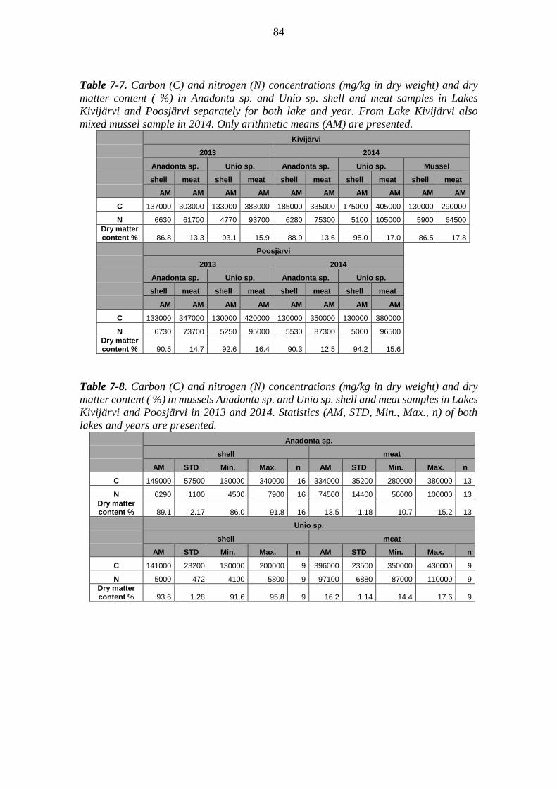
84
Table 7-7. Carbon (C) and nitrogen (N) concentrations (mg/kg in dry weight) and dry
matter content ( %) in Anadonta sp. and Unio sp. shell and meat samples in Lakes
Kivijärvi and Poosjärvi separately for both lake and year. From Lake Kivijärvi also
mixed mussel sample in 2014. Only arithmetic means (AM) are presented.
Kivijärvi
2013 2014
Anadonta sp. Unio sp. Anadonta sp. Unio sp. Mussel
shell meat shell meat shell meat shell meat shell meat
AM AM AM AM AM AM AM AM AM AM
C 137000 303000 133000 383000 185000 335000 175000 405000 130000 290000
N 6630 61700 4770 93700 6280 75300 5100 105000 5900 64500
Dry matter content % 86.8 13.3 93.1 15.9 88.9 13.6 95.0 17.0 86.5 17.8
Poosjärvi 2013 2014 Anadonta sp. Unio sp. Anadonta sp. Unio sp. shell meat shell meat shell meat shell meat AM AM AM AM AM AM AM AM
C 133000 347000 130000 420000 130000 350000 130000 380000 N 6730 73700 5250 95000 5530 87300 5000 96500
Dry matter content % 90.5 14.7 92.6 16.4 90.3 12.5 94.2 15.6
Table 7-8. Carbon (C) and nitrogen (N) concentrations (mg/kg in dry weight) and dry
matter content ( %) in mussels Anadonta sp. and Unio sp. shell and meat samples in Lakes
Kivijärvi and Poosjärvi in 2013 and 2014. Statistics (AM, STD, Min., Max., n) of both
lakes and years are presented.
Anadonta sp.
shell meat
AM STD Min. Max. n AM STD Min. Max. n
C 149000 57500 130000 340000 16 334000 35200 280000 380000 13
N 6290 1100 4500 7900 16 74500 14400 56000 100000 13
Dry matter content % 89.1 2.17 86.0 91.8 16 13.5 1.18 10.7 15.2 13
Unio sp.
shell meat
AM STD Min. Max. n AM STD Min. Max. n
C 141000 23200 130000 200000 9 396000 23500 350000 430000 9
N 5000 472 4100 5800 9 97100 6880 87000 110000 9
Dry matter content % 93.6 1.28 91.6 95.8 9 16.2 1.14 14.4 17.6 9
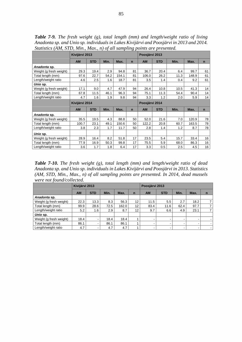
85
Table 7-9. The fresh weight (g), total length (mm) and length/weight ratio of living
Anadonta sp. and Unio sp. individuals in Lakes Kivijärvi and Poosjärvi in 2013 and 2014.
Statistics (AM, STD, Min., Max., n) of all sampling points are presented.
Kivijärvi 2013 Poosjärvi 2013
AM STD Min. Max. n AM STD Min. Max. n
Anadonta sp.
Weight (g fresh weight) 29.3 19.4 2.9 94.8 81 36.7 20.4 6.4 99.7 61
Total length (mm) 97.6 22.7 54.2 154.1 81 106.0 26.2 11.3 148.9 61
Length/weight ratio 4.6 2.5 1.6 18.7 81 3.5 1.4 0.4 9.2 61
Unio sp.
Weight (g fresh weight) 17.1 9.0 4.7 47.9 94 26.4 10.8 10.5 41.3 14
Total length (mm) 67.8 11.5 46.1 96.3 94 75.1 11.3 54.4 90.4 14
Length/weight ratio 4.7 1.6 1.9 9.8 94 3.3 1.2 2.0 5.9 14
Kivijärvi 2014 Poosjärvi 2014
AM STD Min. Max. n AM STD Min. Max. n
Anadonta sp.
Weight (g fresh weight) 35.5 19.5 4.3 88.8 50 52.0 21.6 7.0 120.9 78
Total length (mm) 100.7 23.1 49.1 150.6 50 122.2 20.8 60.7 163.5 78
Length/weight ratio 3.8 2.3 1.7 11.7 50 2.8 1.4 1.2 8.7 78
Unio sp.
Weight (g fresh weight) 28.9 16.4 8.2 51.8 17 23.5 5.4 15.7 33.4 16
Total length (mm) 77.9 16.9 50.3 99.8 17 75.5 5.9 68.0 86.3 16
Length/weight ratio 3.6 1.7 1.8 6.4 17 3.3 0.5 2.5 4.5 16
Table 7-10. The fresh weight (g), total length (mm) and length/weight ratio of dead
Anadonta sp. and Unio sp. individuals in Lakes Kivijärvi and Poosjärvi in 2013. Statistics
(AM, STD, Min., Max., n) of all sampling points are presented. In 2014, dead mussels
were not found/collected.
Kivijärvi 2013 Poosjärvi 2013
AM STD Min. Max. n AM STD Min. Max. n
Anadonta sp.
Weight (g fresh weight) 22.3 13.3 8.3 56.3 12 11.5 5.5 2.7 18.2 7
Total length (mm) 99.9 28.6 72.5 162.0 12 83.4 11.6 62.4 97.7 7
Length/weight ratio 5.2 1.6 2.9 8.7 12 9.7 6.6 4.9 23.1 7
Unio sp.
Weight (g fresh weight) 18.4 - 18.4 18.4 1 - - - - -
Total length (mm) 86.1 - 86.1 86.1 1 - - - - -
Length/weight ratio 4.7 - 4.7 4.7 1 - - - - -

86
7.2.2 Species and biomass of macrobenthos
The number of individuals and the biomass of macrobenthos in Lakes Kivijärvi and
Poosjärvi in autumn 2013 and 2014 are presented in Figures 7-2 and 7-3, respectively. In
these figures, macrobenthos taxa has been divided into five different taxonomic groups;
Oligochaeta, Chironomidae, Ceratopogonidae, Chaoboridae, and Bivalvia. The original
results of macrobenthos determinations and density calculations are presented in
Appendix F-6.
Figure 7-2. The number of macrobenthos individuals of different taxa in Lakes Kivijärvi
and Poosjärvi in September 2013 and October 2014.
Figure 7-3. The biomass of macrobenthos taxa in Lakes Kivijärvi and Poosjärvi in
September 2013 and October 2014.
0
200
400
600
800
1000
1200
1400
18.9.2013 13.10.2014 19.9.2013 15.10.2014
N/m
2
Bivalvia
Chaoboridae
Ceratopogonidae
Chironomidae
Oligochaeta
Kivijärvi Poosjärvi
0,00
0,20
0,40
0,60
0,80
1,00
1,20
1,40
1,60
18.9.2013 13.10.2014 19.9.2013 15.10.2014
g/m
2
Bivalvia
Chaoboridae
Ceratopogonidae
Chironomidae
Oligochaeta
Kivijärvi Poosjärvi

87
7.2.3 Mussels for biomass analysis and dimensions
The summary of the mussel biomass results from Lakes Kivijärvi and Poosjärvi in 2013
and 2014 is presented in Table 7-11. Mean fresh and dry weight of shell and meat of
living and dead mussels, as well as dry matter percentage and meat/shell ratio are
presented. The values were calculated separately for each sampling plot of both lakes.
From each plot three quadrats were sampled, and the mean values for each plot and each
sampling date were first calculated. Finally, the means of all sampling dates and both
years are presented. Fresh and dry weight results are presented as per area. The detailed
results of the mussel biomass measurements for each sampling date, sampling plot, and
quadrat are presented in Appendix F in Table F-5.
The dimensions (length, height, width) of mussel individuals are presented in Table 7-12.
The values for living and dead mussels were calculated separately for each sampling plot.
The means of all sampling dates and both years are presented separately for both lakes.
Table 7-11. The mean (AM) fresh and dry weight of shell and meat, dry matter content of
shell and meat, and meat/shell ratio of living and dead mussels collected from macrophyte
sampling plots in Lakes Kivijärvi and Poosjärvi in 2013 and 2014.
Fresh weight (g/m2)
Dry weight (g/m2)
Dry matter content (%)
Meat/shell ratio
Sampling plot
shell meat shell meat shell meat fresh weight dry weight
Kivijärvi
OA1 living 89 149 74 10 86 6.4 2.4 0.15
dead 49 - 39 - 60 - - -
OA2 living 177 473 144 29 84 6.0 2.7 0.18
dead 20 - 16 - 77 - - -
OA5 living 153 322 99 18 82 6.3 2.7 0.18
dead 17 - 14 - 78 - - -
Poosjärvi
OA2 living 60 132 49 12 81 8.8 2.3 0.24
dead 8 - 6 - 82 - - -
OA3 living 64 125 49 11 79 8.6 2.2 0.21
dead 26 - 18 - 69 - - -
OA4 living 177 337 151 27 86 9.5 1.9 0.18
dead 103 - 78 - 79 - - -
OA7 living 29 81 24 6 82 7.2 3.1 0.28
dead 0 - 0 - - - - -
OA8 living 191 357 161 28 84 8.1 2.2 0.19
dead 193 - 159 - 83 - - -

88
Table 7-12. The dimensions of the mussel individuals collected from macrophyte
sampling plots in Lakes Kivijärvi and Poosjärvi in 2013 and 2014. Arithmetic mean (AM),
standard error (STD), minimum (Min.), maximum (Max.) and number of samples (n) of
each sampling plot are presented separately for both lakes. All the three quadrats per
sampling plot are included.
7.3 Discussion
7.3.1 Element concentrations and concentration ratios of mussels, size data
In living mussels, the concentrations of other key elements except chlorine (Cl), selenium
(Se), and strontium (Sr) were mainly 5–10 times higher in the meat samples compared to
the shell samples. The chlorine and selenium concentrations in meat were 20–40 times
higher than in shells. There were no clear differences in strontium concentrations between
meat and shell samples. In Anadonta sp. meat samples, the concentrations of the other
key elements except Ag and Se were higher compared to Unio sp. meat samples. In shell
samples, no clear trends were observed between Anadonta sp. and Unio sp. samples.
There were no clear differences in element concentrations between the lakes or the years.
There are no previous studies in reference lakes concerning mussels, so there are no
reference data.
The differences in the concentration ratios found for mussels were the same as for the
corresponding concentrations, because the element concentrations in lake water used in
the calculations were the same.
The concentrations of carbon (C) and nitrogen (N) in living Anadonta and Unio meat
samples were higher compared to the shell samples like in most of the key elements. In
Sampling plot
living/dead mussel
Length (cm) Width (cm) Height (cm)
AM STD Min. Max. n AM STD Min. Max. n AM STD Min. Max. n
Kivijärvi
OA1 living 12.80 2.79 9.0 16.1 9 6.87 1.45 5.0 8.6 9 3.58 1.01 2.2 4.8 9
dead 9.71 0.72 8.3 10.6 7 5.24 0.44 4.5 5.9 7 2.86 0.55 2.2 3.5 7
OA2 living 10.24 2.06 6.0 14.5 42 5.63 1.12 2.5 8.0 42 2.84 0.67 1.8 4.4 41
dead 9.90 1.78 7.0 11.9 6 5.13 1.00 4.0 6.5 6 2.55 0.73 1.5 3.4 6
OA5 living 11.34 2.32 5.1 16.0 30 6.21 1.56 2.4 9.3 30 3.15 0.69 1.6 4.8 30
dead 9.67 2.00 7.1 12.0 6 5.33 0.88 4.2 6.3 6 2.58 0.44 2.1 3.2 6
Poosjärvi
OA3 living 11.09 2.41 8.6 15.1 9 6.16 1.21 4.4 8 9 3.29 0.84 2.2 4.8 9
dead 9.22 2.69 6.1 13.4 6 4.83 1.38 3.2 6.9 6 2.75 0.84 1.6 4.0 6
OA4 living 10.23 3.05 6.1 16.0 34 5.53 1.97 2.5 9.5 34 2.99 0.93 1.8 5.1 34
dead 9.72 2.17 6.5 15.0 20 5.08 1.26 3.5 8.5 20 2.96 0.66 1.4 4.0 20
OA7 living 14.20 - 14.2 14.2 1 7.30 - 7.3 7.3 1 4.90 - 4.9 4.9 1
dead - - - - - - - - - - - - - - -
OA8 living 11.26 2.16 7.0 15.0 36 6.09 1.33 3.0 8.5 36 3.20 0.71 2.0 4.6 36
dead 10.31 2.27 6.2 16.5 32 5.45 1.29 3.8 8.2 32 3.14 0.76 1.6 5.3 32
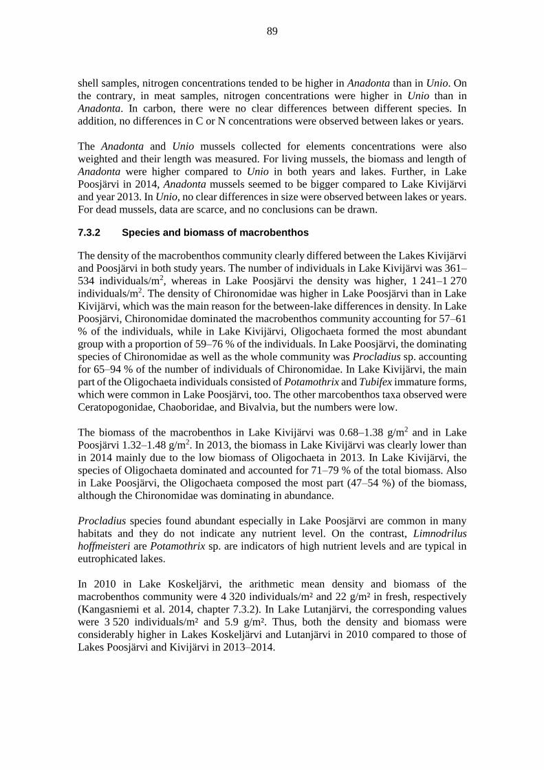
89
shell samples, nitrogen concentrations tended to be higher in Anadonta than in Unio. On
the contrary, in meat samples, nitrogen concentrations were higher in Unio than in
Anadonta. In carbon, there were no clear differences between different species. In
addition, no differences in C or N concentrations were observed between lakes or years.
The Anadonta and Unio mussels collected for elements concentrations were also
weighted and their length was measured. For living mussels, the biomass and length of
Anadonta were higher compared to Unio in both years and lakes. Further, in Lake
Poosjärvi in 2014, Anadonta mussels seemed to be bigger compared to Lake Kivijärvi
and year 2013. In Unio, no clear differences in size were observed between lakes or years.
For dead mussels, data are scarce, and no conclusions can be drawn.
7.3.2 Species and biomass of macrobenthos
The density of the macrobenthos community clearly differed between the Lakes Kivijärvi
and Poosjärvi in both study years. The number of individuals in Lake Kivijärvi was 361–
534 individuals/m2, whereas in Lake Poosjärvi the density was higher, 1 241–1 270
individuals/m2. The density of Chironomidae was higher in Lake Poosjärvi than in Lake
Kivijärvi, which was the main reason for the between-lake differences in density. In Lake
Poosjärvi, Chironomidae dominated the macrobenthos community accounting for 57–61
% of the individuals, while in Lake Kivijärvi, Oligochaeta formed the most abundant
group with a proportion of 59–76 % of the individuals. In Lake Poosjärvi, the dominating
species of Chironomidae as well as the whole community was Procladius sp. accounting
for 65–94 % of the number of individuals of Chironomidae. In Lake Kivijärvi, the main
part of the Oligochaeta individuals consisted of Potamothrix and Tubifex immature forms,
which were common in Lake Poosjärvi, too. The other marcobenthos taxa observed were
Ceratopogonidae, Chaoboridae, and Bivalvia, but the numbers were low.
The biomass of the macrobenthos in Lake Kivijärvi was 0.68–1.38 g/m2 and in Lake
Poosjärvi 1.32–1.48 g/m2. In 2013, the biomass in Lake Kivijärvi was clearly lower than
in 2014 mainly due to the low biomass of Oligochaeta in 2013. In Lake Kivijärvi, the
species of Oligochaeta dominated and accounted for 71–79 % of the total biomass. Also
in Lake Poosjärvi, the Oligochaeta composed the most part (47–54 %) of the biomass,
although the Chironomidae was dominating in abundance.
Procladius species found abundant especially in Lake Poosjärvi are common in many
habitats and they do not indicate any nutrient level. On the contrast, Limnodrilus
hoffmeisteri are Potamothrix sp. are indicators of high nutrient levels and are typical in
eutrophicated lakes.
In 2010 in Lake Koskeljärvi, the arithmetic mean density and biomass of the
macrobenthos community were 4 320 individuals/m² and 22 g/m² in fresh, respectively
(Kangasniemi et al. 2014, chapter 7.3.2). In Lake Lutanjärvi, the corresponding values
were 3 520 individuals/m² and 5.9 g/m². Thus, both the density and biomass were
considerably higher in Lakes Koskeljärvi and Lutanjärvi in 2010 compared to those of
Lakes Poosjärvi and Kivijärvi in 2013–2014.

90
7.3.3 Mussels for biomass analysis and dimensions
Mussels were collected from macrophyte plots to gather data for total biomass and to
calculate biomass distribution for shell and meat. Dimensions (length, height, width) of
the mussels were measured, too. All the living and dead mussels were included, and no
species-specific data were gathered.
In other sampling plots except OA8 in Lake Poosjärvi, the biomass of shells of living
mussels was higher compared to that of dead mussels. In all sampling plot, the number of
living mussels was higher compared to that of dead mussels (see Table 7-12 for n). The
fresh weight of living and dead mussel shells ranged from 29 to 191 g/m2 and from 0 to
193 g/m2, respectively. The fresh weight of living mussel meat ranged from 81 to 473
g/m2. In sampling plot OA8 in Lake Poosjärvi, the fresh weight of living and dead shells
was equal and highest of all plots. The fresh weight of meat was, however, highest in
sampling plot OA2 in Lake Kivijärvi. Dry matter content of shells tended to be higher in
living than in dead mussels ranging from 60 to 86 %.
The mean length of living and dead mussels in sampling plots ranged from 10.2 to 14.2
cm and from 9.2 to 10.31 cm, respectively. The living mussels tended to be longer
compared to dead mussels, but there was noticeable variation in length. The height and
width of all mussels ranged from 4.8 to 7.3 cm and from 2.6 to 4.9 cm, respectively. The
living mussels in some plots were slightly higher and wider compared to dead mussels,
but the differences were minor.
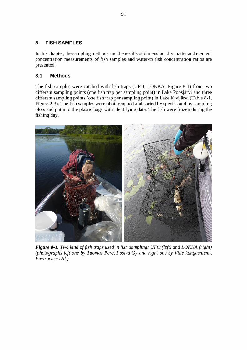
91
8 FISH SAMPLES
In this chapter, the sampling methods and the results of dimension, dry matter and element
concentration measurements of fish samples and water-to fish concentration ratios are
presented.
8.1 Methods
The fish samples were catched with fish traps (UFO, LOKKA; Figure 8-1) from two
different sampling points (one fish trap per sampling point) in Lake Poosjärvi and three
different sampling points (one fish trap per sampling point) in Lake Kivijärvi (Table 8-1,
Figure 2-3). The fish samples were photographed and sorted by species and by sampling
plots and put into the plastic bags with identifying data. The fish were frozen during the
fishing day.
Figure 8-1. Two kind of fish traps used in fish sampling: UFO (left) and LOKKA (right)
(photographs left one by Tuomas Pere, Posiva Oy and right one by Ville kangasniemi,
Envirocase Ltd.).
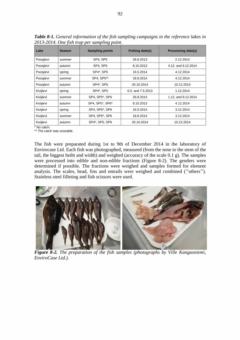
92
Table 8-1. General information of the fish sampling campaigns in the reference lakes in
2013-2014. One fish trap per sampling point.
Lake Season Sampling points Fishing date(s) Processing date(s)
Poosjärvi summer SP4, SP5 26.8.2013 2.12.2014
Poosjärvi autumn SP4, SP5 8.10.2013 4.12. and 9.12.2014
Poosjärvi spring SP4*, SP5 16.5.2014 4.12.2014
Poosjärvi summer SP4, SP5** 18.8.2014 4.12.2014
Poosjärvi autumn SP4*, SP5 20.10.2014 10.12.2014
Kivijärvi spring SP4*, SP5 6.5. and 7.5.2013 1.12.2014
Kivijärvi summer SP4, SP5*, SP6 26.8.2013 1.12. and 9.12.2014
Kivijärvi autumn SP4, SP5*, SP6* 8.10.2013 4.12.2014
Kivijärvi spring SP4, SP5*, SP6 16.5.2014 3.12.2014
Kivijärvi summer SP4, SP5*, SP6 18.8.2014 3.12.2014
Kivijärvi autumn SP4*, SP5, SP6 20.10.2014 10.12.2014
* No catch. ** The catch was unusable.
The fish were preparated during 1st to 9th of December 2014 in the laboratory of
Envirocase Ltd. Each fish was photographed, measured (from the nose to the stem of the
tail, the biggest heiht and width) and weighed (accuracy of the scale 0.1 g). The samples were processed into edible and non-edible fractions (Figure 8-2). The genders were determined if possible. The fractions were weighed and samples formed for element analysis. The scales, head, fins and entrails were weighed and combined (’’others’’). Stainless steel filleting and fish scissors were used. Figure 8-2. The preparation of the fish samples (photographs by Ville Kangasniemi,
EnviroCase Ltd.).
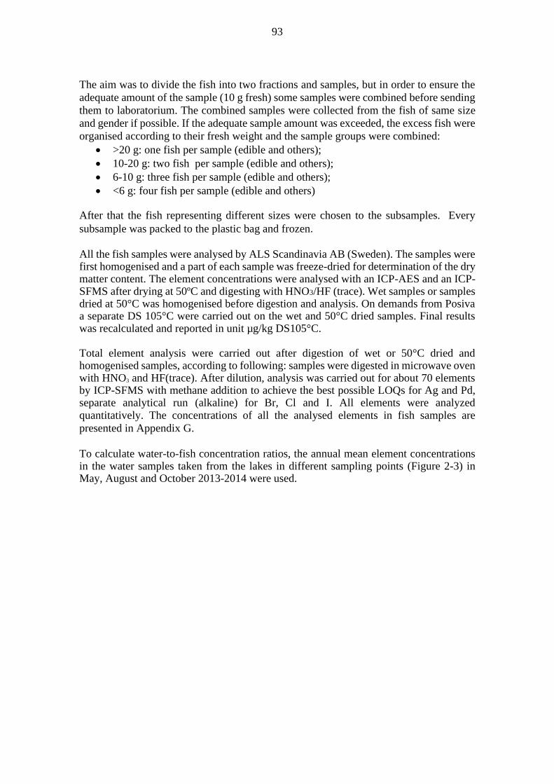
93
The aim was to divide the fish into two fractions and samples, but in order to ensure the
adequate amount of the sample (10 g fresh) some samples were combined before sending
them to laboratorium. The combined samples were collected from the fish of same size
and gender if possible. If the adequate sample amount was exceeded, the excess fish were
organised according to their fresh weight and the sample groups were combined:
>20 g: one fish per sample (edible and others);
10-20 g: two fish per sample (edible and others);
6-10 g: three fish per sample (edible and others);
<6 g: four fish per sample (edible and others)
After that the fish representing different sizes were chosen to the subsamples. Every
subsample was packed to the plastic bag and frozen. All the fish samples were analysed by ALS Scandinavia AB (Sweden). The samples were first homogenised and a part of each sample was freeze-dried for determination of the dry matter content. The element concentrations were analysed with an ICP-AES and an ICP-SFMS after drying at 50ºC and digesting with HNO3/HF (trace). Wet samples or samples dried at 50°C was homogenised before digestion and analysis. On demands from Posiva a separate DS 105°C were carried out on the wet and 50°C dried samples. Final results was recalculated and reported in unit µg/kg DS105°C. Total element analysis were carried out after digestion of wet or 50°C dried and homogenised samples, according to following: samples were digested in microwave oven with HNO3 and HF(trace). After dilution, analysis was carried out for about 70 elements by ICP-SFMS with methane addition to achieve the best possible LOQs for Ag and Pd, separate analytical run (alkaline) for Br, Cl and I. All elements were analyzed quantitatively. The concentrations of all the analysed elements in fish samples are
presented in Appendix G.
To calculate water-to-fish concentration ratios, the annual mean element concentrations in the water samples taken from the lakes in different sampling points (Figure 2-3) in May, August and October 2013-2014 were used.
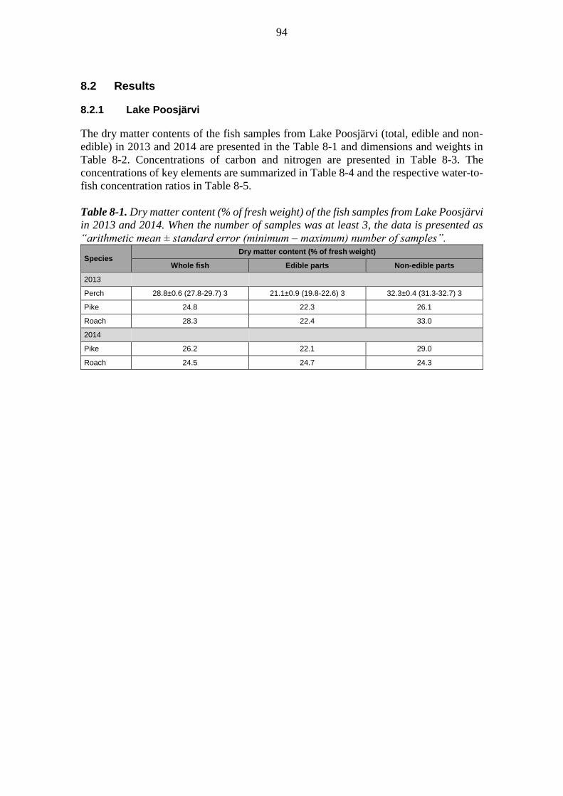
94
8.2 Results
8.2.1 Lake Poosjärvi
The dry matter contents of the fish samples from Lake Poosjärvi (total, edible and non-
edible) in 2013 and 2014 are presented in the Table 8-1 and dimensions and weights in
Table 8-2. Concentrations of carbon and nitrogen are presented in Table 8-3. The
concentrations of key elements are summarized in Table 8-4 and the respective water-to-
fish concentration ratios in Table 8-5.
Table 8-1. Dry matter content (% of fresh weight) of the fish samples from Lake Poosjärvi
in 2013 and 2014. When the number of samples was at least 3, the data is presented as
“arithmetic mean ± standard error (minimum – maximum) number of samples”.
Species Dry matter content (% of fresh weight)
Whole fish Edible parts Non-edible parts
2013
Perch 28.8±0.6 (27.8-29.7) 3 21.1±0.9 (19.8-22.6) 3 32.3±0.4 (31.3-32.7) 3
Pike 24.8 22.3 26.1
Roach 28.3 22.4 33.0
2014
Pike 26.2 22.1 29.0
Roach 24.5 24.7 24.3

95
Table 8-2. The dimensions (cm) of the fish individuals and the respective mass (g) of the whole fish and of the processed fractions of the fish
samples from Lake Poosjärvi in 2013 and 2014. When the number of samples was at least 3, the data is presented as “arithmetic mean ±
standard error (minimum – maximum) number of samples”.
Species Length (cm) Height (cm) Width (cm) Mass (g, fresh) Proportion of edible part
(% of fresh weight) Whole fish Edible parts Non-edible parts
2013
Perch 19.3±1.1 (11-36) 25 4.9±0.4 (2.6-11.0) 25 2.3±0.2 (1.1-5.1) 25 108±28 (12-720) 25 31.5±9.9 (3.9-188.9) 18 76±27 (7-510) 18 30.7±1.1 (23.1-39.6) 18
Pike 59.9±21.0 (21.0-93.1) 3 9.6±3.4 (3.0-14.4) 3 5.6±2.0 (1.8-8.3) 3 2327±1398 (49-4869) 3 815±485 (21-1696) 3 1487±901 (27-3131) 3 43.0±3.8 (39.2-46.8) 3
Roach 14.8 3.3 1.6 29.3 11.5 15.4 39.2
Silver bream 10.8 3.1 1.1 13.4 6.7 6.3 49.8
2014
Perch 13.1 3.2 1.6 32.4 8.9 18.6 34.5
Pike 59.5 8.9 6.1 2193 1004 1358 39.9
Roach 15.8 3.3 1.5 31.0 11.8 17.4 38.1
Table 8-3. Concentrations of carbon and nitrogen in the fish samples (mg/kg, in dry weight) from Lake Poosjärvi in 2013 and 2014.
Species C (mg/kg, dry weight) N (mg/kg, dry weight)
Whole fish Edible parts Non-edible parts Whole fish Edible parts Non-edible parts
2013
Perch 361±4 (353-365) 3 449±6 (440-460) 3 322±6 (310-330) 3 101±2 (97-103) 3 139±6 (130-150) 3 84±2 (80-87) 3
Pike 450 440 455 125 140 117
Roach 401 440 370 100 130 76
2014
Pike 379 450 330 95 139 65
Roach 340 330 350 90 87 93

96
Table 8-4. Concentrations of the analysed key elements in the fish samples (µg/kg, in dry weight) and in the water samples (µg/l) from Lake
Poosjärvi in 2013 and 2014 used to calculate the water-to-fish concentration ratios. The data in grey italics include samples where the
concentration is below the limit of quantification (LOQ), or the result was unreliable; for these, the numerical value of LOQ for fish samples
and LOQ/2 for water samples are used as a surrogate.
Species (number of samples)
Fraction Concentration, µg/l (water) or µg/kg (fishes, dry weight basis)
Ag Cl Cs I Mo Nb Ni Pb Pd Se Sn Sr
2013
Water (6) 5.00E-03 1.95E+03 8.07E-03 3.30E+00 1.09E-01 2.68E-03 1.35E+00 5.37E-02 3.30E-02 1.27E-01 1.00E-02 1.83E+01
Whole fish 1.13E+00 4.49E+06 2.38E+02 3.07E+03 1.41E+01 1.02E+00 4.11E+01 1.68E+02 1.00E+00 1.10E+03 1.81E+01 1.34E+05
Perch (3) Edible parts 1.43E+00 4.41E+06 3.96E+02 2.58E+03 6.42E+00 2.74E-01 6.98E+01 1.65E+01 1.00E+00 1.14E+03 1.54E+01 2.86E+03
Non-edible parts 1.00E+00 4.53E+06 1.68E+02 3.28E+03 1.76E+01 1.35E+00 2.83E+01 2.36E+02 1.00E+00 1.07E+03 1.93E+01 1.92E+05
Whole fish 4.16E+00 4.36E+06 3.53E+02 3.68E+03 3.16E+01 4.56E-01 1.42E+01 1.49E+01 1.00E+00 1.62E+03 2.07E+01 1.06E+04
Pike (2) Edible parts 1.00E+00 3.61E+06 4.56E+02 3.09E+03 4.14E+00 2.00E-01 7.44E+00 4.28E+00 1.00E+00 8.58E+02 1.90E+01 8.91E+02
Non-edible parts 5.35E+00 4.81E+06 2.82E+02 4.59E+03 4.28E+01 5.23E-01 1.77E+01 1.78E+01 1.00E+00 1.96E+03 1.74E+01 1.56E+04
Whole fish 4.41E+00 1.97E+06 1.03E+02 1.10E+03 6.09E+01 2.86E+00 1.19E+02 1.76E+02 1.00E+00 5.21E+02 2.71E+01 3.60E+04
Roach (1) Edible parts 1.88E+00 2.42E+06 1.35E+02 1.23E+03 2.89E+01 4.91E-01 8.69E+01 3.27E+02 1.00E+00 4.72E+02 2.90E+01 6.49E+03
Non-edible parts 6.42E+00 1.61E+06 7.72E+01 9.94E+02 8.64E+01 4.75E+00 1.44E+02 5.54E+01 1.00E+00 5.60E+02 2.55E+01 5.96E+04
2014
Water (9) 6.69E-03 3.22E+03 9.01E-03 3.76E+00 1.37E-01 2.66E-03 1.61E+00 1.75E-02 1.07E-03 5.75E-02 5.62E-03 2.67E+01
Whole fish 4.85E+00 3.20E+06 3.73E+02 4.91E+03 3.09E+01 6.55E-01 1.51E+01 9.53E+01 1.00E+00 1.38E+03 1.65E+01 1.72E+04
Pike (2) Edible parts 1.00E+00 2.29E+06 3.60E+02 2.14E+03 4.71E+00 2.76E-01 1.42E+01 7.30E+00 1.00E+00 8.84E+02 1.16E+01 1.68E+03
Non-edible parts 4.55E+00 2.87E+06 2.11E+02 4.85E+03 3.75E+01 1.12E+00 2.53E+01 1.05E+02 1.00E+00 1.42E+03 1.64E+01 2.70E+04
Whole fish 3.43E+00 3.21E+06 9.16E+01 1.65E+03 9.74E+01 1.39E+01 2.59E+02 2.23E+02 1.00E+00 6.63E+02 1.74E+01 2.70E+05
Roach (1) Edible parts 3.63E+00 2.84E+06 9.25E+01 1.55E+03 1.00E+02 2.00E+01 2.94E+02 3.01E+02 1.00E+00 5.96E+02 1.85E+01 2.88E+05
Non-edible parts 3.22E+00 3.58E+06 9.06E+01 1.76E+03 9.44E+01 7.74E+00 2.23E+02 1.44E+02 1.00E+00 7.31E+02 1.63E+01 2.52E+05

97
Table 8-5. The corresponding water-to-fish concentration ratios (µg/kg)/(µg/l) in dry weight basis, from Lake Poosjärvi in 2013 and 2014.
The data in grey italics include samples where the concentration was below the limit of quantification (LOQ), or the result was unreliable;
for these, the numerical value of LOQ for fish samples and LOQ/2 for water samples are used as a surrogate. When the number of samples
was at least 3, the data is presented as "geomethric mean ± geometric standard deviation (minimun - maximum).
Species (number of samples)
Fraction
Concentration ratio, (µg/kg)/(µg/l), dry weight basis
Ag Cl Cs I Mo Nb Ni Pb Pd Se Sn Sr
2013
Whole fish 226±1.2
(200-287)
2181±1.3 (1630-2734)
29969±1.2 (25811-35222)
917±1.2 (772-1013)
130±1 (125-134)
380±1.2 (337-473)
29±1.4 (21-43)
2577±1.9 (1270-4387)
30±1 (30-30)
8600±1.1 (8069-8926)
1649±1.4 (1092-2047)
6729±1.3 (5809-5833)
Perch (3) Edible parts 265±1.6
(200-463)
2040±1.5 (1433-3038)
49378±1.2 (40133-61512)
798±1.2 (728-947)
52±1.7 (29-87)
97±1.5 (75-155)
45±1.9 (30-96)
313±1.3 (264-424)
30±1 (30-30)
8727±1.3 (6333-10379)
1284±1.9 (629-1946)
127±1.9 (61-191)
Non-edible parts 200±1
(200-200)
2239±1.3 (1728-2607)
21079±1.1 (19844-22227)
966±1.2 (790-1095)
162±1.1 (153-180)
505±1.2 (451-631)
19±1.3 (17-26)
3572±1.9 (1767-6100)
30±1 (30-30)
8501±1.1 (8186-8927)
1791±1.3 (1294-2180)
9686±1.3 (8321-12658)
Whole fish 832 2237 43708 1113 289 171 11 278 30 12759 2069 580
Pike (2) Edible parts 200 1855 56495 934 38 75 5.5 80 30 6758 1902 49
Non-edible parts 1069 2468 34898 1390 392 196 13 331 30 15398 1742 852
Whole fish 881 1010 12730 333 556 1068 88 3274 30 4102 2706 1965
Roach (1) Edible parts 377 1242 16683 374 264 183 65 6081 30 3716 2897 354
Non-edible parts 1285 824 9572 301 790 1775 107 1031 30 4410 2554 3253
2014
Whole fish 725 993 41349 1306 225 247 9.4 5461 934 24027 2947 645
Pike (2) Edible parts 150.0 710 40001 570 34 104 8.8 418 934 15371 2063 63
Non-edible parts 680 892 23382 1290 273 423 16 6025 934 24723 2922 1012
Whole fish 512 997 10164 440 710 5231 160 12757 934 11536 3106 10124
Roach (1) Edible parts 542 882 10272 412 731 7543 182 17227 934 10367 3303 10801
Non-edible parts 482 1113 10055 467 688 2912 138 8273 934 12709 2907 9446
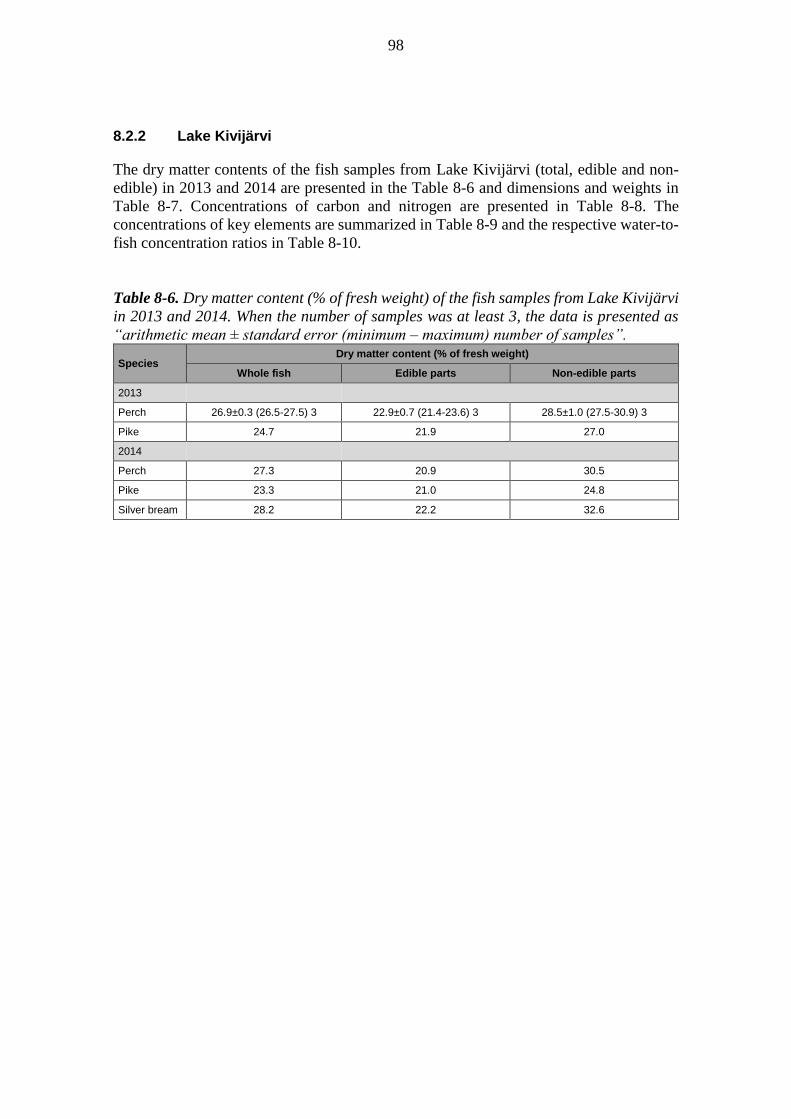
98
8.2.2 Lake Kivijärvi
The dry matter contents of the fish samples from Lake Kivijärvi (total, edible and non-
edible) in 2013 and 2014 are presented in the Table 8-6 and dimensions and weights in
Table 8-7. Concentrations of carbon and nitrogen are presented in Table 8-8. The
concentrations of key elements are summarized in Table 8-9 and the respective water-to-
fish concentration ratios in Table 8-10.
Table 8-6. Dry matter content (% of fresh weight) of the fish samples from Lake Kivijärvi
in 2013 and 2014. When the number of samples was at least 3, the data is presented as
“arithmetic mean ± standard error (minimum – maximum) number of samples”.
Species Dry matter content (% of fresh weight)
Whole fish Edible parts Non-edible parts
2013
Perch 26.9±0.3 (26.5-27.5) 3 22.9±0.7 (21.4-23.6) 3 28.5±1.0 (27.5-30.9) 3
Pike 24.7 21.9 27.0
2014
Perch 27.3 20.9 30.5
Pike 23.3 21.0 24.8
Silver bream 28.2 22.2 32.6

99
Table 8-7. The dimensions (cm) of the fish individuals and the respective mass (g) of the whole fish and of the processed fractions of the fish
samples from Lake Kivijärvi in 2013 and 2014. When the number of samples was at least 3, the data is presented as “arithmetic mean ±
standard error (minimum – maximum) number of samples”.
Species Length (cm) Height (cm) Width (cm) Mass (g, fresh) Proportion of edible part (%
of fresh weight) Whole fish Edible parts Non-edible parts
2013
Perch 12.3±0.4 (8.6-27.9) 58 3.0±0.1 (2.0-8.2) 58 1.4±0.1 (0.8-4.4) 58 24.1±5.4 (5.8-320) 58 9.3±1.7 (2.1-76.6) 33 18.4±5.2 (3.2-235.3) 33 36.6±0.8 (21.5-41.8) 33
Pike 33.8 4.7 3.1 239.8 104.8 131.3 43.7
2014
Perch 11.3±0.6 (79-234) 35 2.6±0.2 (19-63) 35 1.3±0.1 (9.1-29.6) 35 19.0±4.8 (6.1-137) 35 5.7±1.0 (2.2-28.6) 35 12.2±3.6 (3.2-105) 35 36.4±0.9 (20.8-43.1) 35
Pike 52.4 7.6 4.9 1037 415 610 41.7
Roach 106 22.9 10.4 10.0 4.4 4.7 44.0
Silver bream 205 63.3 21.2 95.0 38.2 53.6 40.2
Table 8-8. Concentrations of carbon and nitrogen in the fish samples (mg/kg, in dry weight) from Lake Kivijärvi in 2013 and 2014.
Species C (mg/kg, dry weight) N (mg/kg, dry weight)
Whole fish Edible parts Non-edible parts Whole fish Edible parts Non-edible parts
2013
Perch 403±24 (343-428) 3 439±13 (410-450) 3 387±35 (300-420) 3 107±4 (96-109) 3 134±7 (120-140) 3 95±5 (81-99) 3
Pike 397 442 360 116 136 100.0
2014
Perch 337 435 290 95 125 80
Pike 347 450 280 104 150 74
Silver bream 384 430 350 105 130 87
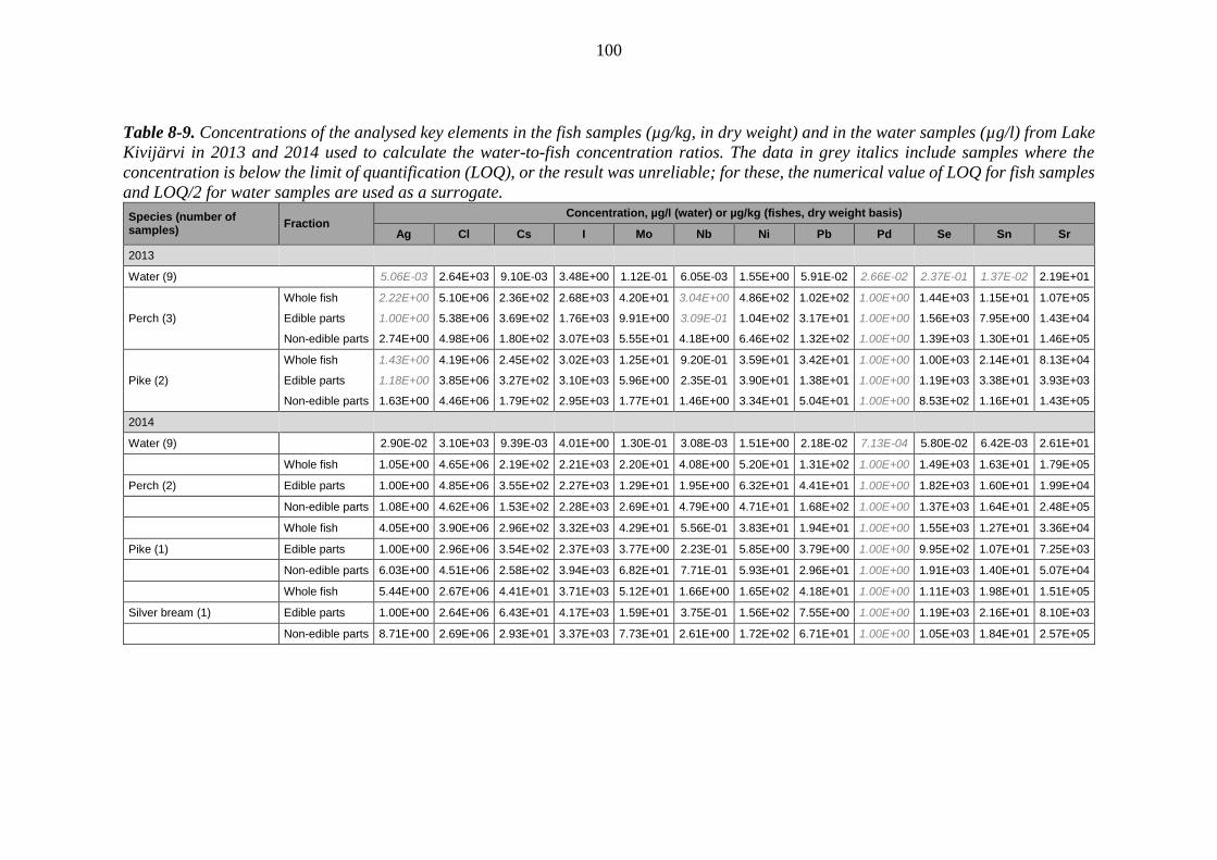
100
Table 8-9. Concentrations of the analysed key elements in the fish samples (µg/kg, in dry weight) and in the water samples (µg/l) from Lake
Kivijärvi in 2013 and 2014 used to calculate the water-to-fish concentration ratios. The data in grey italics include samples where the
concentration is below the limit of quantification (LOQ), or the result was unreliable; for these, the numerical value of LOQ for fish samples
and LOQ/2 for water samples are used as a surrogate.
Species (number of samples)
Fraction Concentration, µg/l (water) or µg/kg (fishes, dry weight basis)
Ag Cl Cs I Mo Nb Ni Pb Pd Se Sn Sr
2013
Water (9) 5.06E-03 2.64E+03 9.10E-03 3.48E+00 1.12E-01 6.05E-03 1.55E+00 5.91E-02 2.66E-02 2.37E-01 1.37E-02 2.19E+01
Whole fish 2.22E+00 5.10E+06 2.36E+02 2.68E+03 4.20E+01 3.04E+00 4.86E+02 1.02E+02 1.00E+00 1.44E+03 1.15E+01 1.07E+05
Perch (3) Edible parts 1.00E+00 5.38E+06 3.69E+02 1.76E+03 9.91E+00 3.09E-01 1.04E+02 3.17E+01 1.00E+00 1.56E+03 7.95E+00 1.43E+04
Non-edible parts 2.74E+00 4.98E+06 1.80E+02 3.07E+03 5.55E+01 4.18E+00 6.46E+02 1.32E+02 1.00E+00 1.39E+03 1.30E+01 1.46E+05
Whole fish 1.43E+00 4.19E+06 2.45E+02 3.02E+03 1.25E+01 9.20E-01 3.59E+01 3.42E+01 1.00E+00 1.00E+03 2.14E+01 8.13E+04
Pike (2) Edible parts 1.18E+00 3.85E+06 3.27E+02 3.10E+03 5.96E+00 2.35E-01 3.90E+01 1.38E+01 1.00E+00 1.19E+03 3.38E+01 3.93E+03
Non-edible parts 1.63E+00 4.46E+06 1.79E+02 2.95E+03 1.77E+01 1.46E+00 3.34E+01 5.04E+01 1.00E+00 8.53E+02 1.16E+01 1.43E+05
2014
Water (9) 2.90E-02 3.10E+03 9.39E-03 4.01E+00 1.30E-01 3.08E-03 1.51E+00 2.18E-02 7.13E-04 5.80E-02 6.42E-03 2.61E+01
Whole fish 1.05E+00 4.65E+06 2.19E+02 2.21E+03 2.20E+01 4.08E+00 5.20E+01 1.31E+02 1.00E+00 1.49E+03 1.63E+01 1.79E+05
Perch (2) Edible parts 1.00E+00 4.85E+06 3.55E+02 2.27E+03 1.29E+01 1.95E+00 6.32E+01 4.41E+01 1.00E+00 1.82E+03 1.60E+01 1.99E+04
Non-edible parts 1.08E+00 4.62E+06 1.53E+02 2.28E+03 2.69E+01 4.79E+00 4.71E+01 1.68E+02 1.00E+00 1.37E+03 1.64E+01 2.48E+05
Whole fish 4.05E+00 3.90E+06 2.96E+02 3.32E+03 4.29E+01 5.56E-01 3.83E+01 1.94E+01 1.00E+00 1.55E+03 1.27E+01 3.36E+04
Pike (1) Edible parts 1.00E+00 2.96E+06 3.54E+02 2.37E+03 3.77E+00 2.23E-01 5.85E+00 3.79E+00 1.00E+00 9.95E+02 1.07E+01 7.25E+03
Non-edible parts 6.03E+00 4.51E+06 2.58E+02 3.94E+03 6.82E+01 7.71E-01 5.93E+01 2.96E+01 1.00E+00 1.91E+03 1.40E+01 5.07E+04
Whole fish 5.44E+00 2.67E+06 4.41E+01 3.71E+03 5.12E+01 1.66E+00 1.65E+02 4.18E+01 1.00E+00 1.11E+03 1.98E+01 1.51E+05
Silver bream (1) Edible parts 1.00E+00 2.64E+06 6.43E+01 4.17E+03 1.59E+01 3.75E-01 1.56E+02 7.55E+00 1.00E+00 1.19E+03 2.16E+01 8.10E+03
Non-edible parts 8.71E+00 2.69E+06 2.93E+01 3.37E+03 7.73E+01 2.61E+00 1.72E+02 6.71E+01 1.00E+00 1.05E+03 1.84E+01 2.57E+05
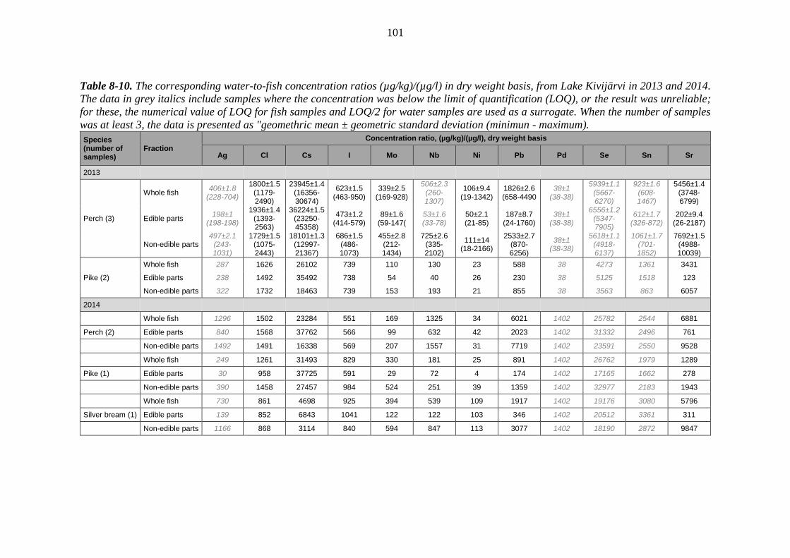
101
Table 8-10. The corresponding water-to-fish concentration ratios (µg/kg)/(µg/l) in dry weight basis, from Lake Kivijärvi in 2013 and 2014.
The data in grey italics include samples where the concentration was below the limit of quantification (LOQ), or the result was unreliable;
for these, the numerical value of LOQ for fish samples and LOQ/2 for water samples are used as a surrogate. When the number of samples
was at least 3, the data is presented as "geomethric mean ± geometric standard deviation (minimun - maximum).
Species (number of samples)
Fraction
Concentration ratio, (µg/kg)/(µg/l), dry weight basis
Ag Cl Cs I Mo Nb Ni Pb Pd Se Sn Sr
2013
Whole fish 406±1.8
(228-704)
1800±1.5 (1179-2490)
23945±1.4 (16356-30674)
623±1.5 (463-950)
339±2.5 (169-928)
506±2.3 (260-1307)
106±9.4 (19-1342)
1826±2.6 (658-4490
38±1 (38-38)
5939±1.1 (5667-6270)
923±1.6 (608-1467)
5456±1.4 (3748-6799)
Perch (3) Edible parts 198±1
(198-198)
1936±1.4 (1393-2563)
36224±1.5 (23250-45358)
473±1.2 (414-579)
89±1.6 (59-147(
53±1.6 (33-78)
50±2.1 (21-85)
187±8.7 (24-1760)
38±1 (38-38)
6556±1.2 (5347-7905)
612±1.7 (326-872)
202±9.4 (26-2187)
Non-edible parts 497±2.1
(243-1031)
1729±1.5 (1075-2443)
18101±1.3 (12997-21367)
686±1.5 (486-1073)
455±2.8 (212-1434)
725±2.6 (335-2102)
111±14 (18-2166)
2533±2.7 (870-6256)
38±1 (38-38)
5618±1.1 (4918-6137)
1061±1.7 (701-1852)
7692±1.5 (4988-10039)
Whole fish 287 1626 26102 739 110 130 23 588 38 4273 1361 3431
Pike (2) Edible parts 238 1492 35492 738 54 40 26 230 38 5125 1518 123
Non-edible parts 322 1732 18463 739 153 193 21 855 38 3563 863 6057
2014
Whole fish 1296 1502 23284 551 169 1325 34 6021 1402 25782 2544 6881
Perch (2) Edible parts 840 1568 37762 566 99 632 42 2023 1402 31332 2496 761
Non-edible parts 1492 1491 16338 569 207 1557 31 7719 1402 23591 2550 9528
Whole fish 249 1261 31493 829 330 181 25 891 1402 26762 1979 1289
Pike (1) Edible parts 30 958 37725 591 29 72 4 174 1402 17165 1662 278
Non-edible parts 390 1458 27457 984 524 251 39 1359 1402 32977 2183 1943
Whole fish 730 861 4698 925 394 539 109 1917 1402 19176 3080 5796
Silver bream (1) Edible parts 139 852 6843 1041 122 122 103 346 1402 20512 3361 311
Non-edible parts 1166 868 3114 840 594 847 113 3077 1402 18190 2872 9847

102
8.3 Discussion
The concentrations and the water-to-fish concentration ratios of key elements for
different fish species vary to some extent. The concentrations of key elements are mainly
rather similar in edible and non-edible parts. They are also at same level in both lakes,
Lake Poosjärvi and Lake Kivijärvi. The concentration of Mo and Sr are smaller in edible
parts of fish than in non-edible parts.
The water-to-fish concentration ratios are mainly at the same level in both lakes between
species, but there are some exceptions. The concentration ratio of Cs for pike is higher
than for other species. Also concentration ratio of Pb for roach is higher than for other
species. Altogether the fish catch was rather scarce and the number of the values below
the limit of quantification is abundant, which can cause uncertainty in the results.
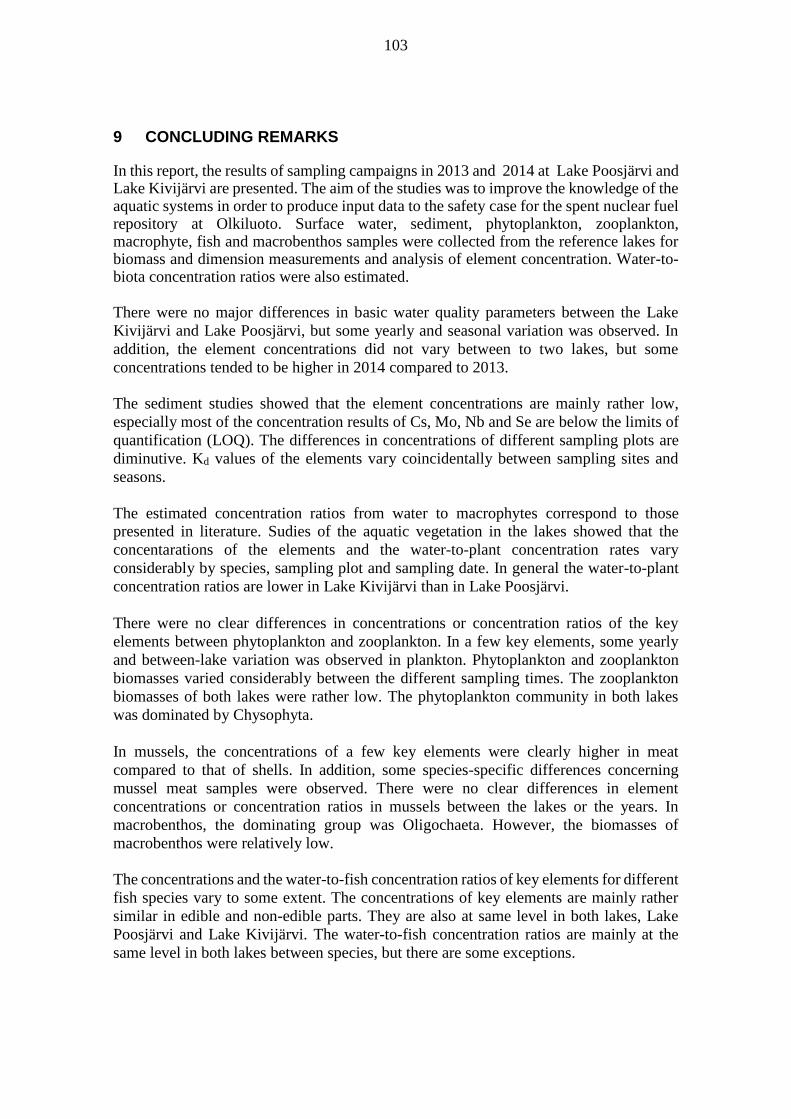
103
9 CONCLUDING REMARKS
In this report, the results of sampling campaigns in 2013 and 2014 at Lake Poosjärvi and Lake Kivijärvi are presented. The aim of the studies was to improve the knowledge of the aquatic systems in order to produce input data to the safety case for the spent nuclear fuel repository at Olkiluoto. Surface water, sediment, phytoplankton, zooplankton, macrophyte, fish and macrobenthos samples were collected from the reference lakes for biomass and dimension measurements and analysis of element concentration. Water-to-biota concentration ratios were also estimated.
There were no major differences in basic water quality parameters between the Lake
Kivijärvi and Lake Poosjärvi, but some yearly and seasonal variation was observed. In
addition, the element concentrations did not vary between to two lakes, but some
concentrations tended to be higher in 2014 compared to 2013.
The sediment studies showed that the element concentrations are mainly rather low,
especially most of the concentration results of Cs, Mo, Nb and Se are below the limits of
quantification (LOQ). The differences in concentrations of different sampling plots are
diminutive. Kd values of the elements vary coincidentally between sampling sites and
seasons.
The estimated concentration ratios from water to macrophytes correspond to those presented in literature. Sudies of the aquatic vegetation in the lakes showed that the
concentarations of the elements and the water-to-plant concentration rates vary
considerably by species, sampling plot and sampling date. In general the water-to-plant
concentration ratios are lower in Lake Kivijärvi than in Lake Poosjärvi.
There were no clear differences in concentrations or concentration ratios of the key
elements between phytoplankton and zooplankton. In a few key elements, some yearly
and between-lake variation was observed in plankton. Phytoplankton and zooplankton
biomasses varied considerably between the different sampling times. The zooplankton
biomasses of both lakes were rather low. The phytoplankton community in both lakes
was dominated by Chysophyta.
In mussels, the concentrations of a few key elements were clearly higher in meat
compared to that of shells. In addition, some species-specific differences concerning
mussel meat samples were observed. There were no clear differences in element
concentrations or concentration ratios in mussels between the lakes or the years. In
macrobenthos, the dominating group was Oligochaeta. However, the biomasses of
macrobenthos were relatively low.
The concentrations and the water-to-fish concentration ratios of key elements for different
fish species vary to some extent. The concentrations of key elements are mainly rather
similar in edible and non-edible parts. They are also at same level in both lakes, Lake
Poosjärvi and Lake Kivijärvi. The water-to-fish concentration ratios are mainly at the
same level in both lakes between species, but there are some exceptions.

104

105
REFERENCES
Areva (1998). Cluff Lake Project Suspension of Operations and Eventual
Decommmisioning of the TMA, Biological Environment. Prepared by Conor Pacific
Environmental Technologies Inc.
Bhupinder, D., Sharmila, P. and Saradhi, P.P. 2009. Potential of Aquatic Macrophytes for
Removing Contaminants from the Environment. Critical Reviews in Environmental
Science and Technology. pp. 754-781.
Dubynin, O.D. (1987). Migration of 129I in a freshwater ecosystem. Ekologiya 5: 91-92.
Engdahl, A., A. Ternsell & S. Hannu (2006). Oskarshamn site investigation – Chemical
characterization of deposits and biota. SKB report P-06-320.
Haapanen, A. (ed.) (2014). Results of monitoring at Olkiluoto in 2012: Environment.
Working report 2013-45, Posiva Oy. Eurajoki, Finland. 180 pp.
Haapanen, R., L. Aro, S. Koivunen, A-M. Lahdenperä, T. Kirkkala, A. Hakala, J. Helin,
& A.T.K. Ikonen (2011). Selection of real-life analogues for future lakes and mires at a
repository site. Radioprotection 46(8): 647-651.
Haapanen R. & A-M. Lahdenperä (2011). Olkiluodon maalta merelle -linjaston
maaosuuden inventointi vuonna 2008 ja Olkiluodon ympäristön ruovikkotutkimukset
vuosina 2007-2008 (in Finnish with an English abstract: The inventory of the terrestrial
part of land-to-sea transects on Olkiluoto Island in 2008 and the investigations of reedbeds
surrounding Olkiluoto Island carried out in 2007-2008). Working report 2011-67, Posiva
Oy. Eurajoki, Finland.
Haapanen, R., L. Aro, T. Kirkkala, S. Koivunen, A-M. Lahdenperä & A. Paloheimo
(2010). Potential reference mires and lakes for biosphere assessment of Olkiluoto site.
Working report 2010-67, Posiva Oy. Eurajoki, Finland.
Haapanen, R., L. Aro, J. Helin, T. Hjerpe, A.T.K. Ikonen, T. Kirkkala, S. Koivunen, A-
M. Lahdenperä, L. Puhakka, M. Rinne & T. Salo (2009). Olkiluoto biosphere description
2009. Report POSIVA 2009-02. Posiva Oy. Eurajoki, Finland.
Haavisto, F. & M. Toivola (2017). Studies on the aquatic environment at Olkiluoto and
Reference area: 6. Reference rivers 2014-2015. Working report 2017-13, Posiva Oy.
Eurajoki, Finland.
Hakila, R. & P. Kalinainen (2001). Poosjärven luonto, linnusto ja kasvillisuus vuonna
2001. Raportti vedennoston vaikutuksista Noormarkun kunnalle (in Finnish: The nature,
birdlife and flora of Lake Poosjärvi in 2001 – Report of the effects of water level raising
to the Noormarkku municipality).
Hakila, R. & P. Kalinainen (1992). Poosjärven luonto, linnusto ja kasvillisuus vuonna
1992 (in Finnsih: The nature, birdlife and flora of Lake Poosjärvi in 1992).

106
Hosseini, A., H. Thørring, J.E. Brown, R. Saxén & E. Ilus (2008). Transfer of
radionuclides in aquatic ecosystems – Default concentration ratios for aquatic biota in the
Erica Tool. Journal of Environmental Radioactivity 99: 1408-1429.
Kangasniemi, V., A.T.K. Ikonen & J. Mustonen (2016). Studies on the aquatic
environment at Olkiluoto and reference area: 2. Reference lakes in 2011-2012. Working
report 2016-50, Posiva Oy. Eurajoki, Finland.
Kangasniemi, V. & J. Helin (2014). Studies on the aquatic environment at Olkiluoto and
reference area: 1. Olkiluoto reference lakes and Eurajoki and Lapijoki Rivers in 2009-
2010. Working report 2013-65, Posiva Oy. Eurajoki, Finland.
Kangasniemi, V., J. Helin, T. Kirkkala & A.T.K. Ikonen (2011). Concentration ratios to
aquatic plants at and near Olkiluoto repository site. Radioprotection 46: 6, 29-34.
Kirkkala, T., E. Mikkilä & S. Koivunen (2017). Studies on the aquatic environment at
Olkiluoto and Reference area: 3. Olkiluoto in 2011-2012. Working report 2016-64,
Posiva Oy. Eurajoki, Finland.
Lepistö, K. (2015). Porin Kivijärven vesikasvikartoitus kesällä 2013 (in Finnish with an
English abstract: Survey of floating-leaved macrophytes in Lake Kivijärvi (Western
Finland), summer 2013). Working report 2015-38, Posiva Oy. Eurajoki, Finland.
Lusa, M. 2017. Sorption experiments of Ag, Cl, Cs, I, Mo, Ni, Pb, Se, Sn, Sr and Tc –
Lastensuo bog samples and Poosjärvi and Kivijärvi sediment samples. Working report
2017-35, Posiva Oy. Eurajoki, Finland.
Ojala, A.E.K. (2011). Sedimenttistratigafia ja sedimentaatioympäristön muutokset
Itämerestä kuroutuneissa järvissä Satakunnassa (in Finnish with an English abstract:
Sediment lithostratigraphy and past changes in sedimentary environment in isolated lakes
in Satakunta region). Working report 2011-87, Posiva Oy. Eurajoki, Finland.
Posiva Oy (2014). Safety case for the disposal of spent nuclear at Olkiluoto: Data basis
for the biosphere assessment BSA 2012. Report POSIVA 2012-28, Posiva Oy. Eurajoki,
Finland.
Posiva (2013a). Olkiluoto biosphere description 2012. Report POSIVA 2012-06, Posiva
Oy. Eurajoki, Finland.
Posiva (2013b). Safety case for the disposal of spent nuclear fuel at Olkiluoto: Terrain
and ecosystem development modelling in the biosphere assessment BSA-2012. Report
POSIVA 2012-29, Posiva Oy. Eurajoki, Finland.
Poutanen, M. (2011). Present bedrock movements and land uplift. In: Ikonen, A.T.K &
T. Lipping (eds.) Proceedings of a seminar on sea level displacement and bedrock uplift
(10th to 11th of June 2010, Pori, Finland). Working report 2011-07, pp. 25-35. Posiva Oy.
Eurajoki, Finland.

107
SFS (Suomen standardoimisliitto) 2006. SFS-EN 15204, Water quality – Guidance
standard on the enumeration of phytoplankton using inverted microscopy (Utermöhl
technique). 42 pp.
Sheppard, S.C., J.M. Long & B. Sanipelli (2010). Measured elemental transfer factors for
boreal hunter/gatherer scenarios: fish, game and berries. Journal of Environmental
Radioactivity 101(11): 902-909.
Sheppard, S., J. Long, B. Sanipelli & G. Sohlenius (2009). Solid/liquid partition
coefficients (Kd) for selected soils and sediments at Forsmark and Laxemar-Simpevarp.
Report R-09-27. Swedish Nuclear Fuel and Waste Management Co., 78 pp. Stockholm.
Sheppard, M.I., S.C. Sheppard & C.A. Grant (2007). Solid/liquid partition coefficients to
model trace element critical loads for agricultural soils in Canada. Canadian Journal of
Soil Science 87: 189-201.
Vintsukevich, N.V. & Y.U.A. Tomilin (1987). Radionuclide distribution in aquatic
system (NPP cooling pond-river-sea estuary). Ekologiya 6: 72.
Viro, P. J. (1952). Kivisyyden määrittämisestä (in Finnish with English summary: On the
determination of stoniness). Communicationes Instituti Forestalis Fenniae 40: 3, 1-23.
Yankovich, T.L. (2010). Compilation of Concentration Ratios for Aquatic Non-human
Biota Collected by the Canadian Power Reactors Sector. CANDU Owners Group Inc.

108

109
APPENDICES
APPENDIX A: Sampling locations
Table A-1. Coordinates of sampling locations in Lake Poosjärvi (OL-TMA71) in 2013
and 2014. The coordinate data is presented in the ETRS89/ETRS-TM35FIN system. The
accuracy of the data may vary considerably.
Poosjärvi
OL-TMA71 Type
Dominating species
ETRS-TM35FIN
Sampling plot N E
OA3 macrophytes horsetail 6846233 228450
OA4 macrophytes yellow water-lily 6846176 228542
OA5-SP1 macrophytes mixed 6845300 229502
OA5-SP2 macrophytes mixed 6845309 229502
OA5-SP3 macrophytes mixed 6845335 229503
OA5-SP4 macrophytes mixed 6845336 229490
OA5-SP5 macrophytes mixed 6845350 229473
OA5-SP6 macrophytes mixed 6845343 229454
OA6 macrophytes floating pondweed 6845468 229459
OA7 macrophytes horsetail 6845252 228730
OA8 macrophytes yellow water-lily 6845142 228723
OA10-SP1 macrophytes bulrush 6843965 229888
OA10-SP2 macrophytes bulrush 6843978 229876
OA10-SP3 macrophytes bulrush 6843992 229903
OA11-SP1 macrophytes sedge 6843928 229788
OA11-SP2 macrophytes sedge 6843959 229793
OA11-SP3 macrophytes sedge 6843987 229802
OA12-SP1 macrophytes marsh cinquefoil 6845197 229514
OA12-SP2 macrophytes marsh cinquefoil 6845187 229523
OA12-SP3 macrophytes marsh cinquefoil 6845178 229529
SP1 water 6846365 228554
SP2 water 6845302 229264
SP3 water 6844067 230053
SP4 fish 6844461 229775
SP5 fish 6844021 230074
SP8 plankton and water 6844738 228943
SP9 macrobenthos 6844609 229307
SP10 macrobenthos 6845138 228892
SP11 macrobenthos 6845646 228974
SP12 macrobenthos 6844366 230059
SP16 water 6843976 229848

110
Table A-2. Coordinates of sampling locations in Lake Kivijärvi (OL-TMA73) in 2013 and
2014. The coordinate data is presented in the ETRS89/ETRS-TM35FIN system. The
accuracy of the data may vary considerably.
Kivijärvi
OL-TMA73 Type
Dominating species
ETRS-TM35FIN
Sampling plot N E
OA1 macrophytes yellow water-lily 6848733 223497
OA2 macrophytes yellow water-lily 6848675 223996
OA3-SP1 macrophytes common reed 6848413 224362
OA3-SP2 macrophytes common reed 6848407 224372
OA3-SP3 macrophytes common reed 6848407 224379
OA3-SP4 macrophytes common reed 6848390 224362
OA3-SP5 macrophytes common reed 6848387 224380
OA3-SP6 macrophytes common reed 6848390 224383
OA4 macrophytes bulrush 6848322 223966
OA5 macrophytes yellow water-lily 6848067 224427
OA6-SP1 macrophytes sedge 6847879 224481
OA6-SP2 macrophytes sedge 6847892 224469
OA6-SP3 macrophytes sedge 6847920 224433
OA7-SP1 macrophytes sedge 6848027 223886
OA7-SP2 macrophytes sedge 6848022 223912
OA7-SP3 macrophytes sedge 6848013 223932
SP1 water 6848472 223786
SP2 water 6848178 224292
SP3 water 6847984 224002
SP4 fish 6848206 223993
SP5 fish 6848456 223795
SP6 fish 6848733 223509
SP7 plankton and water 6848599 223818
SP10 macrobenthos 6848666 223730
SP11 macrobenthos 6848459 223870
SP12 macrobenthos 6848267 224244
SP13 macrobenthos 6848109 223998
APPENDIX B: Water samples (Excel)
APPENDIX C: Sediment samples (Excel)
APPENDIX D: Macrophytes (Excel)
APPENDIX E: Plankton (Excel)
APPENDIX F: Macrobenthos (Excel)
APPENDIX G: Fish samples (Excel)

SAMPLE: 18176PLACE: POSIOMA , Kivijärvi N EDATE: 18.9.2013DEPTH: 0.00- 2.00 m
COUNTED BY Lounais-Suomen vesi- ja ympäristötutkimus Oy, SA ON 10/24/2013
CHAMBER VOLUME=10ml, DIAM=26mm
BIOMASS OF PHYTOPLANKTON COUNTED WITH Leica DMI3000 B:400 units in 64 Kenttiä at 788x53 units in 50 Kenttiä at 500x484 units in 1 Pohja at 125x
COMMENT: - pikoplanktonia
Species Size A/H Volume Units Coeff. Units/l Units % ww µg/l ww %
2 21 CHROOCOCCALES 4 5 30 16266 487980 6.96 2.44 0.302 21 CHROOCOCCALES 7 10 7 16266 113862 1.62 1.14 0.142 21 CHROOCOCCALES 9 19 3 16266 48798 0.70 0.93 0.112 21 CHROOCOCCALES 11 26 7 16266 113862 1.62 2.96 0.362 21 CHROOCOCCALES 14 47 1 16266 16266 0.23 0.76 0.092 21 CYANODICTYON PLANCTONICUM HIC 2 cf. 50 1 8633 8633 0.12 0.43 0.052 21 MERISMOPEDIA SP. 1 1 11 16266 178926 2.55 0.18 0.022 21 SNOWELLA SP. 1 10 4 16266 65064 0.93 0.65 0.082 21 SNOWELLA SP. 3 42 3 16266 48798 0.70 2.05 0.254 0 CRYPTOMONADALES 3 94 1 16266 16266 0.23 1.53 0.194 0 CRYPTOMONADALES 4 151 2 16266 32532 0.46 4.91 0.604 0 CRYPTOMONADALES 8 1884 1 8633 8633 0.12 16.26 1.974 0 CRYPTOMONAS SP. 2 754 12 8633 103596 1.48 78.11 9.484 0 CRYPTOMONAS SP. 3 1769 3 8633 25899 0.37 45.82 5.564 0 KATABLEPHARIS OVALIS SKUJA 1 HET 92 2 16266 32532 0.46 2.99 0.364 0 RHODOMONAS LACUSTRIS PASCH.&R 2 82 22 16266 357852 5.10 29.34 3.564 0 RHODOMONAS LACUSTRIS PASCH.&R 3 122 1 16266 16266 0.23 1.98 0.245 0 DINOPHYCEAE 1 105 1 16266 16266 0.23 1.71 0.215 0 DINOPHYCEAE 5 2010 2 8633 17266 0.25 34.70 4.215 0 DINOPHYCEAE 6 4421 1 8633 8633 0.12 38.17 4.636 61 BICOSOECA SP. HET 67 1 16266 16266 0.23 1.09 0.136 63 CHRYSOLYKOS PLANCTONICUS MACK 105 1 16266 16266 0.23 1.71 0.216 63 CHRYSOPHYCEAE 2 180 3 16266 48798 0.70 8.78 1.076 63 DINOBRYON BAVARICUM IMH. 226 4 8633 34532 0.49 7.80 0.956 63 DINOBRYON BORGEI LEMM. 16 2 16266 32532 0.46 0.52 0.066 63 DINOBRYON DIVERGENS IMH. 153 388 100 38800 0.55 5.94 0.726 63 DINOBRYON SP. 1 47 2 16266 32532 0.46 1.53 0.196 63 KEPHYRION SP. 92 3 16266 48798 0.70 4.49 0.546 63 MALLOMONAS SP. 3 335 1 16266 16266 0.23 5.45 0.666 63 MALLOMONAS TONSURATA TEIL. 1 670 1 8633 8633 0.12 5.78 0.706 63 PSEUDOPEDINELLA SP. 2 65 6 16266 97596 1.39 6.34 0.776 63 PSEUDOPEDINELLA SP. 3 132 1 16266 16266 0.23 2.15 0.266 63 SPINIFEROMONAS SP. 1 65 3 16266 48798 0.70 3.17 0.396 63 SPINIFEROMONAS SP. 2 180 7 16266 113862 1.62 20.50 2.496 63 SYNURA SP. 2 1055 4 8633 34532 0.49 36.43 4.426 65 AULACOSEIRA SP. 2 755 1 8633 8633 0.12 6.52 0.796 65 AULACOSEIRA TENELLA (NYGAARD) 141 2 16266 32532 0.46 4.59 0.566 65 BACILLARIALES 2 135 2 8633 17266 0.25 2.33 0.286 65 BACILLARIALES 10 2640 1 100 100 0.00 0.26 0.036 65 RHIZOSOLENIA LONGISETA ZACH. 1 1319 4 8633 34532 0.49 45.55 5.536 65 TABELLARIA SP. 2 1750 3 100 300 0.00 0.53 0.066 66 TRIBOPHYCEAE 226 1 16266 16266 0.23 3.68 0.456 67 GONYOSTOMUM SEMEN (EHR.) DIES. 1 9538 4 100 400 0.01 3.82 0.466 67 GONYOSTOMUM SEMEN (EHR.) DIES. 2 18652 2 100 200 0.00 3.73 0.456 67 GONYOSTOMUM SP. 1 1444 35 100 3500 0.05 5.05 0.617 71 EUGLENA HEMICHROMATA SKUJA cf. 10718 13 100 1300 0.02 13.93 1.697 71 EUGLENA SP. 1 3224 2 100 200 0.00 0.64 0.087 71 EUGLENA SP. 2 5828 2 100 200 0.00 1.17 0.147 71 EUGLENA SPIROGYRA EHR. 2177 1 100 100 0.00 0.22 0.037 71 EUGLENA TRIPTERIS (DUJ.) KLEBS 2 cf. 4689 7 100 700 0.01 3.28 0.407 71 PHACUS CURVICAUDA SVIR. 4875 11 100 1100 0.02 5.36 0.657 71 PHACUS LONGICAUDA (EHR.) DUJ. 1 8164 5 100 500 0.01 4.08 0.507 71 PHACUS SP. 2 3266 3 100 300 0.00 0.98 0.127 71 PHACUS SP. 3 6029 1 100 100 0.00 0.60 0.077 71 TRACHELOMONAS SP. 1 904 1 8633 8633 0.12 7.80 0.957 73 PYRAMIMONAS SP. 3 132 1 16266 16266 0.23 2.15 0.267 74 CHLOROPHYCEAE 1 113 4 16266 65064 0.93 7.35 0.897 74 DICTYOSPHAERIUM PULCHELLUM WO 452 8 8633 69064 0.98 31.22 3.797 74 GOLENKINIA RADIATA CHOD. 697 1 16266 16266 0.23 11.34 1.387 74 MICRACTINIUM PUSILLUM FRES. 368 1 8633 8633 0.12 3.18 0.397 74 MONOMASTIX SP. 1 31 4 16266 65064 0.93 2.02 0.247 74 MONORAPHIDIUM SP. 1 10 3 16266 48798 0.70 0.49 0.067 74 OOCYSTIS SP. 1 59 6 16266 97596 1.39 5.76 0.707 74 PEDIASTRUM ANGULOSUM (EHR.) ME 1 22687 1 100 100 0.00 2.27 0.287 74 PEDIASTRUM DUPLEX V. GRACILLIM 5024 3 100 300 0.00 1.51 0.187 74 PEDIASTRUM PRIVUM (PRINTZ) HEG 1 452 1 8633 8633 0.12 3.90 0.477 74 PEDIASTRUM SP. 5652 2 100 200 0.00 1.13 0.147 74 PEDIASTRUM TETRAS (EHR.) RALFS 2 1809 1 8633 8633 0.12 15.62 1.907 74 SCENEDESMUS ARMATUS CHOD. 1 170 1 16266 16266 0.23 2.77 0.347 74 SCENEDESMUS BICELLULARIS 75 8 16266 130128 1.86 9.76 1.18
APPENDIX E-5: Phytoplankton species and biomass111

7 74 SCENEDESMUS SP. 5 264 1 8633 8633 0.12 2.28 0.287 74 SPERMATOZOPSIS EXULTANS KORSH 19 15 16266 243990 3.48 4.64 0.567 74 TETRAEDRON SP. 211 1 16266 16266 0.23 3.43 0.427 74 VOLVOCALES 5 410 1 16266 16266 0.23 6.67 0.819 92 FLAGELLATES SPP. AUTO (OVAL) 2 5 8 16266 130128 1.86 0.65 0.089 92 FLAGELLATES SPP. AUTO (OVAL) 3 19 22 16266 357852 5.10 6.80 0.839 92 FLAGELLATES SPP. AUTO (OVAL) 4 64 5 16266 81330 1.16 5.21 0.639 92 FLAGELLATES SPP. AUTO (OVAL) 5 181 6 16266 97596 1.39 17.66 2.149 92 FLAGELLATES SPP. AUTO (OVAL) 7 1579 3 8633 25899 0.37 40.89 4.969 92 FLAGELLATES SPP. AUTO (SPHERE) 2 8 29 16266 471714 6.73 3.77 0.469 92 FLAGELLATES SPP. AUTO (SPHERE) 3 33 16 16266 260256 3.71 8.59 1.049 92 FLAGELLATES SPP. AUTO (SPHERE) 4 113 3 16266 48798 0.70 5.51 0.679 92 MONAD AUTOTROPHIC 1 6 12 16266 195192 2.78 1.17 0.149 92 MONAD AUTOTROPHIC 2 14 59 16266 959694 13.69 13.44 1.639 92 MONAD AUTOTROPHIC 3 24 26 16266 422916 6.03 10.15 1.239 92 MONAD AUTOTROPHIC 4 65 26 16266 422916 6.03 27.49 3.349 92 MONAD AUTOTROPHIC 5 92 3 16266 48798 0.70 4.49 0.549 92 MONAD AUTOTROPHIC 6 180 5 16266 81330 1.16 14.64 1.789 92 MONAD AUTOTROPHIC 7 188 2 16266 32532 0.46 6.12 0.749 92 MONAD AUTOTROPHIC 8 502 1 8633 8633 0.12 4.33 0.539 92 MONAD AUTOTROPHIC 9 523 5 16266 81330 1.16 42.54 5.16
2 CYANOPHYTA - CYANOPHYCEAE 67 1082189 15.43 11.54 1.402 21 CHROOCOCCALES 67 1082189 15.43 11.54 1.404 CRYPTOPHYTA 44 593576 8.46 180.95 21.975 DINOPHYTA 4 42165 0.60 74.58 9.056 CHRYSOPHYTA 482 718206 10.24 187.73 22.796 61 BICOSOECOPHYCEAE 1 16266 0.23 1.09 0.136 63 CHRYSOPHYCEAE 426 588211 8.39 110.59 13.426 65 DIATOMOPHYCEAE 13 93363 1.33 59.77 7.266 66 TRIBOPHYCEAE 1 16266 0.23 3.68 0.456 67 RAPHIDOPHYCEAE 41 4100 0.06 12.60 1.537 CHLOROPHYTA 109 849299 12.11 155.54 18.887 71 EUGLENOPHYCEAE 46 13133 0.19 38.08 4.627 73 PRASINOPHYCEAE 1 16266 0.23 2.15 0.267 74 CHLOROPHYCEAE 62 819900 11.69 115.31 14.009 OTHER PHYTOPLANKTON 231 3726914 53.15 213.45 25.919 92 MONADS AND FLAGELLATES 231 3726914 53.15 213.45 25.91
Total counted: 937 7012349 823.79
Total autotrophs: 934 6963551 99.30 819.71 99.50Total heterotrophs: 3 48798 0.70 4.08 0.50
112
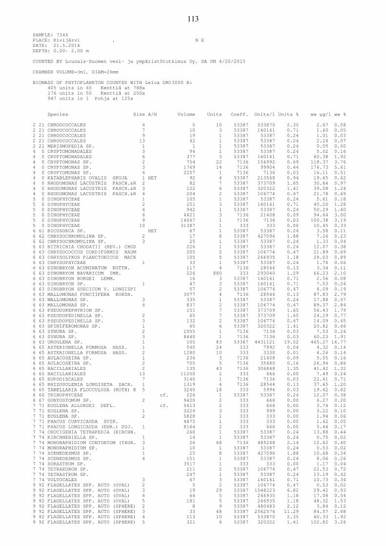
SAMPLE: 7344PLACE: Kivijärvi , N EDATE: 21.5.2014DEPTH: 0.00- 2.00 m
COUNTED BY Lounais-Suomen vesi- ja ympäristötutkimus Oy, SA ON 4/20/2015
CHAMBER VOLUME=3ml, DIAM=26mm
BIOMASS OF PHYTOPLANKTON COUNTED WITH Leica DMI3000 B:405 units in 65 Kenttiä at 788x176 units in 50 Kenttiä at 250x947 units in 1 Pohja at 125x
Species Size A/H Volume Units Coeff. Units/l Units % ww µg/l ww %
2 21 CHROOCOCCALES 4 5 10 53387 533870 2.35 2.67 0.082 21 CHROOCOCCALES 7 10 3 53387 160161 0.71 1.60 0.052 21 CHROOCOCCALES 9 19 1 53387 53387 0.24 1.01 0.032 21 CHROOCOCCALES 13 42 1 53387 53387 0.24 2.24 0.072 21 MERISMOPEDIA SP. 1 1 1 53387 53387 0.24 0.05 0.004 0 CRYPTOMONADALES 3 94 1 53387 53387 0.24 5.02 0.164 0 CRYPTOMONADALES 6 377 3 53387 160161 0.71 60.38 1.924 0 CRYPTOMONAS SP. 2 754 22 7136 156992 0.69 118.37 3.764 0 CRYPTOMONAS SP. 3 1769 14 7136 99904 0.44 176.73 5.614 0 CRYPTOMONAS SP. 4 2257 1 7136 7136 0.03 16.11 0.514 0 KATABLEPHARIS OVALIS SKUJA 1 HET 92 4 53387 213548 0.94 19.65 0.624 0 RHODOMONAS LACUSTRIS PASCH.&R 2 82 7 53387 373709 1.65 30.64 0.974 0 RHODOMONAS LACUSTRIS PASCH.&R 3 122 6 53387 320322 1.41 39.08 1.244 0 RHODOMONAS LACUSTRIS PASCH.&R 4 204 2 53387 106774 0.47 21.78 0.695 0 DINOPHYCEAE 1 105 1 53387 53387 0.24 5.61 0.185 0 DINOPHYCEAE 2 251 3 53387 160161 0.71 40.20 1.285 0 DINOPHYCEAE 4 942 1 53387 53387 0.24 50.29 1.605 0 DINOPHYCEAE 6 4421 3 7136 21408 0.09 94.64 3.005 0 DINOPHYCEAE 9 14067 1 7136 7136 0.03 100.38 3.195 0 DINOPHYCEAE 10 31387 1 333 333 0.00 10.45 0.336 61 BICOSOECA SP. HET 67 1 53387 53387 0.24 3.58 0.116 62 CHRYSOCHROMULINA SP. 2 17 8 53387 427096 1.88 7.26 0.236 62 CHRYSOCHROMULINA SP. 3 25 1 53387 53387 0.24 1.33 0.046 63 BITRICHIA CHODATII (REV.) CHOD 226 1 53387 53387 0.24 12.07 0.386 63 CHRYSOCOCCUS CORDIFORMIS NAUM 205 2 53387 106774 0.47 21.89 0.696 63 CHRYSOLYKOS PLANCTONICUS MACK 105 5 53387 266935 1.18 28.03 0.896 63 CHRYSOPHYCEAE 1 33 1 53387 53387 0.24 1.76 0.066 63 DINOBRYON ACUMINATUM RUTTN. 117 4 7136 28544 0.13 3.34 0.116 63 DINOBRYON BAVARICUM IMH. 226 880 333 293040 1.29 66.23 2.106 63 DINOBRYON BORGEI LEMM. 16 3 53387 160161 0.71 2.56 0.086 63 DINOBRYON SP. 1 47 3 53387 160161 0.71 7.53 0.246 63 DINOBRYON SUECICUM V. LONGISPI 57 2 53387 106774 0.47 6.09 0.196 63 MALLOMONAS PUNCTIFERA KORSH. 3077 4 7136 28544 0.13 87.83 2.796 63 MALLOMONAS SP. 3 335 1 53387 53387 0.24 17.88 0.576 63 MALLOMONAS SP. 4 837 2 53387 106774 0.47 89.37 2.846 63 PSEUDOKEPHYRION SP. 151 7 53387 373709 1.65 56.43 1.796 63 PSEUDOPEDINELLA SP. 2 65 7 53387 373709 1.65 24.29 0.776 63 PSEUDOPEDINELLA SP. 3 132 2 53387 106774 0.47 14.09 0.456 63 SPINIFEROMONAS SP. 1 65 6 53387 320322 1.41 20.82 0.666 63 SYNURA SP. 2 1055 1 7136 7136 0.03 7.53 0.246 63 SYNURA SP. 3 8440 1 7136 7136 0.03 60.23 1.916 63 UROGLENA SP. 1 105 83 53387 4431121 19.52 465.27 14.776 65 ASTERIONELLA FORMOSA HASS. 1 540 24 333 7992 0.04 4.32 0.146 65 ASTERIONELLA FORMOSA HASS. 2 1280 10 333 3330 0.01 4.26 0.146 65 AULACOSEIRA SP. 1 236 3 7136 21408 0.09 5.05 0.166 65 AULACOSEIRA SP. 2 755 5 7136 35680 0.16 26.94 0.866 65 BACILLARIALES 2 135 43 7136 306848 1.35 41.42 1.326 65 BACILLARIALES 13 11250 2 333 666 0.00 7.49 0.246 65 EUPODISCALES 7 3140 1 7136 7136 0.03 22.41 0.716 65 RHIZOSOLENIA LONGISETA ZACH. 1 1319 4 7136 28544 0.13 37.65 1.206 65 TABELLARIA FLOCCULOSA (ROTH) K 5 3240 18 333 5994 0.03 19.42 0.626 66 TRIBOPHYCEAE cf. 226 1 53387 53387 0.24 12.07 0.386 67 GONYOSTOMUM SP. 2 9420 2 333 666 0.00 6.27 0.207 71 EUGLENA ALLORGEI DEFL. cf. 5613 2 333 666 0.00 3.74 0.127 71 EUGLENA SP. 1 3224 3 333 999 0.00 3.22 0.107 71 EUGLENA SP. 2 5828 1 333 333 0.00 1.94 0.067 71 PHACUS CURVICAUDA SVIR. 4875 1 333 333 0.00 1.62 0.057 71 PHACUS LONGICAUDA (EHR.) DUJ. 1 8164 2 333 666 0.00 5.44 0.177 74 CRUCIGENIA TETRAPEDIA (KIRCHN. 260 1 53387 53387 0.24 13.88 0.447 74 KIRCHNERIELLA SP. 1 14 1 53387 53387 0.24 0.75 0.027 74 MONORAPHIDIUM CONTORTUM (THUR. 3 26 68 7136 485248 2.14 12.62 0.407 74 MONORAPHIDIUM SP. 1 10 1 53387 53387 0.24 0.53 0.027 74 SCENEDESMUS SP. 1 25 8 53387 427096 1.88 10.68 0.347 74 SCENEDESMUS SP. 4 151 1 53387 53387 0.24 8.06 0.267 74 SORASTRUM SP. 3517 1 333 333 0.00 1.17 0.047 74 TETRAEDRON SP. 211 2 53387 106774 0.47 22.53 0.727 74 TETRASTRUM SP. 247 1 53387 53387 0.24 13.19 0.427 74 VOLVOCALES 3 67 3 53387 160161 0.71 10.73 0.349 92 FLAGELLATES SPP. AUTO (OVAL) 2 5 2 53387 106774 0.47 0.53 0.029 92 FLAGELLATES SPP. AUTO (OVAL) 3 19 29 53387 1548223 6.82 29.42 0.939 92 FLAGELLATES SPP. AUTO (OVAL) 4 64 5 53387 266935 1.18 17.08 0.549 92 FLAGELLATES SPP. AUTO (OVAL) 5 181 5 53387 266935 1.18 48.32 1.539 92 FLAGELLATES SPP. AUTO (SPHERE) 2 8 9 53387 480483 2.12 3.84 0.129 92 FLAGELLATES SPP. AUTO (SPHERE) 3 33 48 53387 2562576 11.29 84.57 2.689 92 FLAGELLATES SPP. AUTO (SPHERE) 4 113 10 53387 533870 2.35 60.33 1.929 92 FLAGELLATES SPP. AUTO (SPHERE) 5 321 6 53387 320322 1.41 102.82 3.26
113
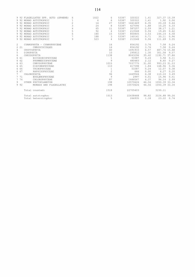
9 92 FLAGELLATES SPP. AUTO (SPHERE) 6 1022 6 53387 320322 1.41 327.37 10.399 92 MONAD AUTOTROPHIC 1 6 6 53387 320322 1.41 1.92 0.069 92 MONAD AUTOTROPHIC 2 14 27 53387 1441449 6.35 20.18 0.649 92 MONAD AUTOTROPHIC 3 24 8 53387 427096 1.88 10.25 0.339 92 MONAD AUTOTROPHIC 4 65 11 53387 587257 2.59 38.17 1.219 92 MONAD AUTOTROPHIC 5 92 4 53387 213548 0.94 19.65 0.629 92 MONAD AUTOTROPHIC 6 180 15 53387 800805 3.53 144.14 4.589 92 MONAD AUTOTROPHIC 7 188 3 53387 160161 0.71 30.11 0.969 92 MONAD AUTOTROPHIC 9 523 4 53387 213548 0.94 111.69 3.55
2 CYANOPHYTA - CYANOPHYCEAE 16 854192 3.76 7.58 0.242 21 CHROOCOCCALES 16 854192 3.76 7.58 0.244 CRYPTOPHYTA 60 1491933 6.57 487.76 15.485 DINOPHYTA 10 295812 1.30 301.58 9.576 CHRYSOPHYTA 1138 8043296 35.42 1192.71 37.866 61 BICOSOECOPHYCEAE 1 53387 0.24 3.58 0.116 62 PRYMNESIOPHYCEAE 9 480483 2.12 8.60 0.276 63 CHRYSOPHYCEAE 1015 7037775 31.00 993.23 31.536 65 DIATOMOPHYCEAE 110 417598 1.84 168.96 5.366 66 TRIBOPHYCEAE 1 53387 0.24 12.07 0.386 67 RAPHIDOPHYCEAE 2 666 0.00 6.27 0.207 CHLOROPHYTA 96 1449544 6.38 110.10 3.497 71 EUGLENOPHYCEAE 9 2997 0.01 15.96 0.517 74 CHLOROPHYCEAE 87 1446547 6.37 94.14 2.999 OTHER PHYTOPLANKTON 198 10570626 46.56 1050.39 33.349 92 MONADS AND FLAGELLATES 198 10570626 46.56 1050.39 33.34
Total counted: 1518 22705403 3150.11
Total autotrophs: 1513 22438468 98.82 3126.88 99.26Total heterotrophs: 5 266935 1.18 23.22 0.74
114
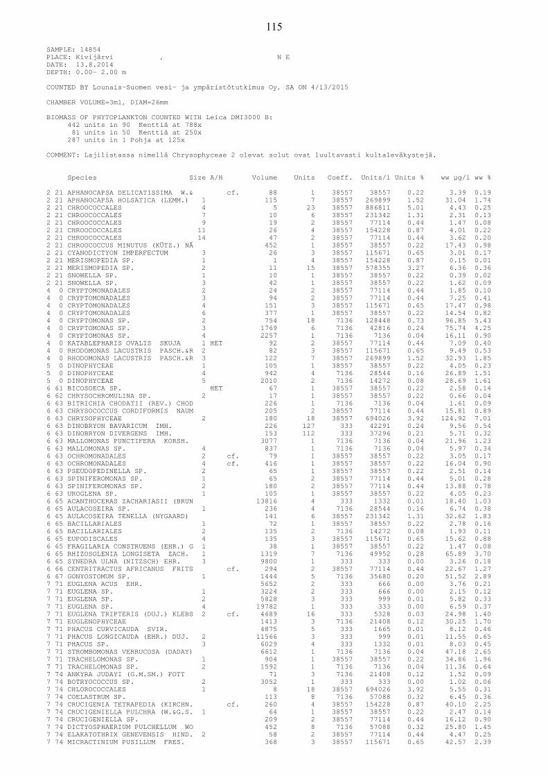
SAMPLE: 14854PLACE: Kivijärvi , N EDATE: 13.8.2014DEPTH: 0.00- 2.00 m
COUNTED BY Lounais-Suomen vesi- ja ympäristötutkimus Oy, SA ON 4/13/2015
CHAMBER VOLUME=3ml, DIAM=26mm
BIOMASS OF PHYTOPLANKTON COUNTED WITH Leica DMI3000 B:442 units in 90 Kenttiä at 788x81 units in 50 Kenttiä at 250x
287 units in 1 Pohja at 125x
COMMENT: Lajilistassa nimellä Chrysophyceae 2 olevat solut ovat luultavasti kultaleväkystejä.
Species Size A/H Volume Units Coeff. Units/l Units % ww µg/l ww %
2 21 APHANOCAPSA DELICATISSIMA W.& cf. 88 1 38557 38557 0.22 3.39 0.192 21 APHANOCAPSA HOLSATICA (LEMM.) 1 115 7 38557 269899 1.52 31.04 1.742 21 CHROOCOCCALES 4 5 23 38557 886811 5.01 4.43 0.252 21 CHROOCOCCALES 7 10 6 38557 231342 1.31 2.31 0.132 21 CHROOCOCCALES 9 19 2 38557 77114 0.44 1.47 0.082 21 CHROOCOCCALES 11 26 4 38557 154228 0.87 4.01 0.222 21 CHROOCOCCALES 14 47 2 38557 77114 0.44 3.62 0.202 21 CHROOCOCCUS MINUTUS (KÜTZ.) NÄ 452 1 38557 38557 0.22 17.43 0.982 21 CYANODICTYON IMPERFECTUM 3 26 3 38557 115671 0.65 3.01 0.172 21 MERISMOPEDIA SP. 1 1 4 38557 154228 0.87 0.15 0.012 21 MERISMOPEDIA SP. 2 11 15 38557 578355 3.27 6.36 0.362 21 SNOWELLA SP. 1 10 1 38557 38557 0.22 0.39 0.022 21 SNOWELLA SP. 3 42 1 38557 38557 0.22 1.62 0.094 0 CRYPTOMONADALES 2 24 2 38557 77114 0.44 1.85 0.104 0 CRYPTOMONADALES 3 94 2 38557 77114 0.44 7.25 0.414 0 CRYPTOMONADALES 4 151 3 38557 115671 0.65 17.47 0.984 0 CRYPTOMONADALES 6 377 1 38557 38557 0.22 14.54 0.824 0 CRYPTOMONAS SP. 2 754 18 7136 128448 0.73 96.85 5.434 0 CRYPTOMONAS SP. 3 1769 6 7136 42816 0.24 75.74 4.254 0 CRYPTOMONAS SP. 4 2257 1 7136 7136 0.04 16.11 0.904 0 KATABLEPHARIS OVALIS SKUJA 1 HET 92 2 38557 77114 0.44 7.09 0.404 0 RHODOMONAS LACUSTRIS PASCH.&R 2 82 3 38557 115671 0.65 9.49 0.534 0 RHODOMONAS LACUSTRIS PASCH.&R 3 122 7 38557 269899 1.52 32.93 1.855 0 DINOPHYCEAE 1 105 1 38557 38557 0.22 4.05 0.235 0 DINOPHYCEAE 4 942 4 7136 28544 0.16 26.89 1.515 0 DINOPHYCEAE 5 2010 2 7136 14272 0.08 28.69 1.616 61 BICOSOECA SP. HET 67 1 38557 38557 0.22 2.58 0.146 62 CHRYSOCHROMULINA SP. 2 17 1 38557 38557 0.22 0.66 0.046 63 BITRICHIA CHODATII (REV.) CHOD 226 1 7136 7136 0.04 1.61 0.096 63 CHRYSOCOCCUS CORDIFORMIS NAUM 205 2 38557 77114 0.44 15.81 0.896 63 CHRYSOPHYCEAE 2 180 18 38557 694026 3.92 124.92 7.016 63 DINOBRYON BAVARICUM IMH. 226 127 333 42291 0.24 9.56 0.546 63 DINOBRYON DIVERGENS IMH. 153 112 333 37296 0.21 5.71 0.326 63 MALLOMONAS PUNCTIFERA KORSH. 3077 1 7136 7136 0.04 21.96 1.236 63 MALLOMONAS SP. 4 837 1 7136 7136 0.04 5.97 0.346 63 OCHROMONADALES 2 cf. 79 1 38557 38557 0.22 3.05 0.176 63 OCHROMONADALES 4 cf. 416 1 38557 38557 0.22 16.04 0.906 63 PSEUDOPEDINELLA SP. 2 65 1 38557 38557 0.22 2.51 0.146 63 SPINIFEROMONAS SP. 1 65 2 38557 77114 0.44 5.01 0.286 63 SPINIFEROMONAS SP. 2 180 2 38557 77114 0.44 13.88 0.786 63 UROGLENA SP. 1 105 1 38557 38557 0.22 4.05 0.236 65 ACANTHOCERAS ZACHARIASII (BRUN 13816 4 333 1332 0.01 18.40 1.036 65 AULACOSEIRA SP. 1 236 4 7136 28544 0.16 6.74 0.386 65 AULACOSEIRA TENELLA (NYGAARD) 141 6 38557 231342 1.31 32.62 1.836 65 BACILLARIALES 1 72 1 38557 38557 0.22 2.78 0.166 65 BACILLARIALES 2 135 2 7136 14272 0.08 1.93 0.116 65 EUPODISCALES 4 135 3 38557 115671 0.65 15.62 0.886 65 FRAGILARIA CONSTRUENS (EHR.) G 1 38 1 38557 38557 0.22 1.47 0.086 65 RHIZOSOLENIA LONGISETA ZACH. 1 1319 7 7136 49952 0.28 65.89 3.706 65 SYNEDRA ULNA (NITZSCH) EHR. 3 9800 1 333 333 0.00 3.26 0.186 66 CENTRITRACTUS AFRICANUS FRITS cf. 294 2 38557 77114 0.44 22.67 1.276 67 GONYOSTOMUM SP. 1 1444 5 7136 35680 0.20 51.52 2.897 71 EUGLENA ACUS EHR. 5652 2 333 666 0.00 3.76 0.217 71 EUGLENA SP. 1 3224 2 333 666 0.00 2.15 0.127 71 EUGLENA SP. 2 5828 3 333 999 0.01 5.82 0.337 71 EUGLENA SP. 4 19782 1 333 333 0.00 6.59 0.377 71 EUGLENA TRIPTERIS (DUJ.) KLEBS 2 cf. 4689 16 333 5328 0.03 24.98 1.407 71 EUGLENOPHYCEAE 1413 3 7136 21408 0.12 30.25 1.707 71 PHACUS CURVICAUDA SVIR. 4875 5 333 1665 0.01 8.12 0.467 71 PHACUS LONGICAUDA (EHR.) DUJ. 2 11566 3 333 999 0.01 11.55 0.657 71 PHACUS SP. 3 6029 4 333 1332 0.01 8.03 0.457 71 STROMBOMONAS VERRUCOSA (DADAY) 6612 1 7136 7136 0.04 47.18 2.657 71 TRACHELOMONAS SP. 1 904 1 38557 38557 0.22 34.86 1.967 71 TRACHELOMONAS SP. 2 1592 1 7136 7136 0.04 11.36 0.647 74 ANKYRA JUDAYI (G.M.SM.) FOTT 71 3 7136 21408 0.12 1.52 0.097 74 BOTRYOCOCCUS SP. 2 3052 1 333 333 0.00 1.02 0.067 74 CHLOROCOCCALES 1 8 18 38557 694026 3.92 5.55 0.317 74 COELASTRUM SP. 113 8 7136 57088 0.32 6.45 0.367 74 CRUCIGENIA TETRAPEDIA (KIRCHN. cf. 260 4 38557 154228 0.87 40.10 2.257 74 CRUCIGENIELLA PULCHRA (W.&G.S. 1 64 1 38557 38557 0.22 2.47 0.147 74 CRUCIGENIELLA SP. 209 2 38557 77114 0.44 16.12 0.907 74 DICTYOSPHAERIUM PULCHELLUM WO 452 8 7136 57088 0.32 25.80 1.457 74 ELAKATOTHRIX GENEVENSIS HIND. 2 58 2 38557 77114 0.44 4.47 0.257 74 MICRACTINIUM PUSILLUM FRES. 368 3 38557 115671 0.65 42.57 2.39
115

7 74 MONOMASTIX SP. 1 31 4 38557 154228 0.87 4.78 0.277 74 MONORAPHIDIUM SP. 1 10 3 38557 115671 0.65 1.16 0.067 74 OOCYSTIS SP. 1 cf. 59 2 38557 77114 0.44 4.55 0.267 74 OOCYSTIS SP. 2 cf. 196 2 38557 77114 0.44 15.11 0.857 74 PEDIASTRUM ANGULOSUM (EHR.) ME 1 22687 1 333 333 0.00 7.55 0.427 74 PEDIASTRUM BORYANUM (TURP.) ME 20096 1 333 333 0.00 6.69 0.387 74 PEDIASTRUM DUPLEX MEYEN 1 1963 1 7136 7136 0.04 14.01 0.797 74 PEDIASTRUM DUPLEX MEYEN 3 9499 1 333 333 0.00 3.16 0.187 74 PEDIASTRUM DUPLEX MEYEN 5 17663 1 333 333 0.00 5.88 0.337 74 PEDIASTRUM DUPLEX V. GRACILLIM 5024 1 333 333 0.00 1.67 0.097 74 PEDIASTRUM TETRAS (EHR.) RALFS 2 1809 2 7136 14272 0.08 25.82 1.457 74 SCENEDESMUS SP. 1 25 61 38557 2351977 13.29 58.80 3.307 74 SCENEDESMUS SP. 2 50 3 38557 115671 0.65 5.78 0.327 74 SCENEDESMUS SP. 6 301 1 38557 38557 0.22 11.61 0.657 74 SCENEDESMUS SUBSPICATUS CHOD. 2 cf. 301 1 38557 38557 0.22 11.61 0.657 74 SPERMATOZOPSIS EXULTANS KORSH cf. 19 18 38557 694026 3.92 13.19 0.747 74 TETRAEDRON CAUDATUM (CORDA) HA 1 139 1 38557 38557 0.22 5.36 0.307 74 TETRASTRUM KOMAREKII HIND. 100 10 38557 385570 2.18 38.56 2.167 74 VOLVOCALES 3 67 4 38557 154228 0.87 10.33 0.587 75 STAURASTRUM SP. 3 3157 1 333 333 0.00 1.05 0.067 75 TEILINGIA GRANULATA (ROY&BISS. 239 1 38557 38557 0.22 9.22 0.529 92 FLAGELLATES SPP. AUTO (OVAL) 2 5 4 38557 154228 0.87 0.77 0.049 92 FLAGELLATES SPP. AUTO (OVAL) 3 19 19 38557 732583 4.14 13.92 0.789 92 FLAGELLATES SPP. AUTO (OVAL) 4 64 11 38557 424127 2.40 27.14 1.529 92 FLAGELLATES SPP. AUTO (OVAL) 5 181 1 38557 38557 0.22 6.98 0.399 92 FLAGELLATES SPP. AUTO (SPHERE) 2 8 7 38557 269899 1.52 2.16 0.129 92 FLAGELLATES SPP. AUTO (SPHERE) 3 33 26 38557 1002482 5.66 33.08 1.869 92 FLAGELLATES SPP. AUTO (SPHERE) 4 113 1 38557 38557 0.22 4.36 0.249 92 FLAGELLATES SPP. AUTO (SPHERE) 5 321 2 38557 77114 0.44 24.75 1.399 92 MONAD AUTOTROPHIC 1 6 3 38557 115671 0.65 0.69 0.049 92 MONAD AUTOTROPHIC 2 14 22 38557 848254 4.79 11.88 0.679 92 MONAD AUTOTROPHIC 3 24 21 38557 809697 4.57 19.43 1.099 92 MONAD AUTOTROPHIC 4 65 33 38557 1272381 7.19 82.70 4.649 92 MONAD AUTOTROPHIC 5 92 8 38557 308456 1.74 28.38 1.599 92 MONAD AUTOTROPHIC 6 180 8 38557 308456 1.74 55.52 3.11
2 CYANOPHYTA - CYANOPHYCEAE 70 2698990 15.25 79.23 4.442 21 CHROOCOCCALES 70 2698990 15.25 79.23 4.444 CRYPTOPHYTA 45 949540 5.36 279.31 15.675 DINOPHYTA 7 81373 0.46 59.62 3.346 CHRYSOPHYTA 308 1889059 10.67 456.20 25.596 61 BICOSOECOPHYCEAE 1 38557 0.22 2.58 0.146 62 PRYMNESIOPHYCEAE 1 38557 0.22 0.66 0.046 63 CHRYSOPHYCEAE 270 1180591 6.67 230.07 12.916 65 DIATOMOPHYCEAE 29 518560 2.93 148.69 8.346 66 TRIBOPHYCEAE 2 77114 0.44 22.67 1.276 67 RAPHIDOPHYCEAE 5 35680 0.20 51.52 2.897 CHLOROPHYTA 212 5682085 32.10 596.61 33.477 71 EUGLENOPHYCEAE 42 86225 0.49 194.65 10.927 74 CHLOROPHYCEAE 168 5556970 31.39 391.69 21.977 75 CONJUGATOPHYCEAE 2 38890 0.22 10.27 0.589 OTHER PHYTOPLANKTON 166 6400462 36.16 311.77 17.499 92 MONADS AND FLAGELLATES 166 6400462 36.16 311.77 17.49
Total counted: 808 17701509 1782.74
Total autotrophs: 805 17585838 99.35 1773.07 99.46Total heterotrophs: 3 115671 0.65 9.68 0.54
116
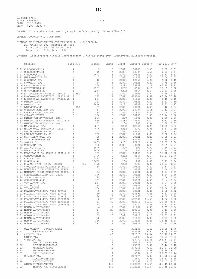
SAMPLE: 19552PLACE: Kivijärvi , N EDATE: 7.10.2014DEPTH: 0.00- 2.00 m
COUNTED BY Lounais-Suomen vesi- ja ympäristötutkimus Oy, SA ON 4/14/2015
CHAMBER VOLUME=5ml, DIAM=26mm
BIOMASS OF PHYTOPLANKTON COUNTED WITH Leica DMI3000 B:235 units in 100 Kenttiä at 788x34 units in 50 Kenttiä at 250x24 units in 1 Pohja at 125x
COMMENT: Lajilistassa nimellä Chrysophyceae 2 olevat solut ovat luultavasti kultaleväkystejä.
Species Size A/H Volume Units Coeff. Units/l Units % ww µg/l ww %
2 21 CHROOCOCCALES 4 5 5 20821 104105 2.07 0.52 0.092 21 CHROOCOCCALES 7 10 4 20821 83284 1.65 0.83 0.142 21 CHROOCOCCUS SP. 1072 1 20821 20821 0.41 22.32 3.812 21 MERISMOPEDIA SP. 1 1 2 20821 41642 0.83 0.04 0.012 21 SNOWELLA SP. 3 42 3 20821 62463 1.24 2.62 0.452 21 SNOWELLA SP. 5 84 1 20821 20821 0.41 1.75 0.304 0 CRYPTOMONAS SP. 2 754 14 4282 59948 1.19 45.20 7.714 0 CRYPTOMONAS SP. 3 1769 2 4282 8564 0.17 15.15 2.584 0 CRYPTOMONAS SP. 4 2257 2 4282 8564 0.17 19.33 3.304 0 KATABLEPHARIS OVALIS SKUJA 1 HET 92 5 20821 104105 2.07 9.58 1.634 0 RHODOMONAS LACUSTRIS PASCH.&R 3 122 24 20821 499704 9.92 60.96 10.404 0 RHODOMONAS LACUSTRIS PASCH.&R 4 204 2 20821 41642 0.83 8.49 1.455 0 DINOPHYCEAE 2 251 1 20821 20821 0.41 5.23 0.895 0 DINOPHYCEAE 5 2010 1 4282 4282 0.08 8.61 1.476 61 BICOSOECA SP. HET 67 1 20821 20821 0.41 1.40 0.246 62 CHRYSOCHROMULINA SP. 2 17 4 20821 83284 1.65 1.42 0.246 62 CHRYSOCHROMULINA SP. 3 25 2 20821 41642 0.83 1.04 0.186 63 CHRYSOPHYCEAE 2 180 5 20821 104105 2.07 18.74 3.206 63 DINOBRYON BAVARICUM IMH. 226 8 200 1600 0.03 0.36 0.066 63 DINOBRYON CRENULATUM W.&G.S.W 410 2 4282 8564 0.17 3.51 0.606 63 DINOBRYON DIVERGENS IMH. 153 9 200 1800 0.04 0.28 0.056 63 MALLOMONAS SP. 4 837 3 4282 12846 0.25 10.75 1.836 63 MALLOMONAS TONSURATA TEIL. 1 670 1 4282 4282 0.08 2.87 0.496 63 PSEUDOPEDINELLA SP. 2 65 4 20821 83284 1.65 5.41 0.926 63 PSEUDOPEDINELLA SP. 3 132 2 20821 41642 0.83 5.50 0.946 63 SPINIFEROMONAS SP. 1 65 1 20821 20821 0.41 1.35 0.236 63 SPINIFEROMONAS SP. 2 180 3 20821 62463 1.24 11.24 1.926 63 SYNURA SP. 2 1055 4 4282 17128 0.34 18.07 3.086 63 UROGLENA SP. 1 105 1 20821 20821 0.41 2.19 0.376 65 AULACOSEIRA SP. 3 1570 4 200 800 0.02 1.26 0.216 65 BACILLARIALES 11 4000 1 200 200 0.00 0.80 0.146 65 FRAGILARIA CONSTRUENS (EHR.) G 2 151 5 20821 104105 2.07 15.72 2.686 67 GONYOSTOMUM SP. 2 9420 2 4282 8564 0.17 80.67 13.767 71 EUGLENA SP. 2 5828 1 200 200 0.00 1.17 0.207 71 EUGLENA SP. 3 18652 1 200 200 0.00 3.73 0.647 71 PHACUS PYRUM (EHR.) STEIN cf. 5495 1 4282 4282 0.08 23.53 4.017 74 CRUCIGENIELLA PULCHRA (W.&G.S. 1 64 1 20821 20821 0.41 1.33 0.237 74 MONORAPHIDIUM CONTORTUM (THUR. 1 9 1 4282 4282 0.08 0.04 0.017 74 MONORAPHIDIUM CONTORTUM (THUR. 3 26 1 20821 20821 0.41 0.54 0.097 74 SCENEDESMUS ARMATUS CHOD. 1 170 1 20821 20821 0.41 3.54 0.607 74 SCENEDESMUS SP. 1 25 2 20821 41642 0.83 1.04 0.187 74 SCENEDESMUS SP. 4 151 1 20821 20821 0.41 3.14 0.547 74 TETRASTRUM SP. 247 1 20821 20821 0.41 5.14 0.887 74 VOLVOCALES 2 35 1 20821 20821 0.41 0.73 0.127 74 VOLVOCALES 6 904 2 20821 41642 0.83 37.64 6.429 92 FLAGELLATES SPP. AUTO (OVAL) 2 5 1 20821 20821 0.41 0.10 0.029 92 FLAGELLATES SPP. AUTO (OVAL) 3 19 19 20821 395599 7.85 7.52 1.289 92 FLAGELLATES SPP. AUTO (OVAL) 4 64 3 20821 62463 1.24 4.00 0.689 92 FLAGELLATES SPP. AUTO (SPHERE) 2 8 28 20821 582988 11.57 4.66 0.809 92 FLAGELLATES SPP. AUTO (SPHERE) 3 33 39 20821 812019 16.11 26.80 4.579 92 FLAGELLATES SPP. AUTO (SPHERE) 4 113 7 20821 145747 2.89 16.47 2.819 92 MONAD AUTOTROPHIC 1 6 2 20821 41642 0.83 0.25 0.049 92 MONAD AUTOTROPHIC 2 14 22 20821 458062 9.09 6.41 1.099 92 MONAD AUTOTROPHIC 3 24 9 20821 187389 3.72 4.50 0.779 92 MONAD AUTOTROPHIC 4 65 10 20821 208210 4.13 13.53 2.319 92 MONAD AUTOTROPHIC 5 92 2 20821 41642 0.83 3.83 0.659 92 MONAD AUTOTROPHIC 6 180 6 20821 124926 2.48 22.49 3.849 92 MONAD AUTOTROPHIC 9 523 1 20821 20821 0.41 10.89 1.86
2 CYANOPHYTA - CYANOPHYCEAE 16 333136 6.61 28.09 4.792 21 CHROOCOCCALES 16 333136 6.61 28.09 4.794 CRYPTOPHYTA 49 722527 14.34 158.72 27.075 DINOPHYTA 2 25103 0.50 13.83 2.366 CHRYSOPHYTA 62 638772 12.68 182.57 31.146 61 BICOSOECOPHYCEAE 1 20821 0.41 1.40 0.246 62 PRYMNESIOPHYCEAE 6 124926 2.48 2.46 0.426 63 CHRYSOPHYCEAE 43 379356 7.53 80.27 13.696 65 DIATOMOPHYCEAE 10 105105 2.09 17.78 3.036 67 RAPHIDOPHYCEAE 2 8564 0.17 80.67 13.767 CHLOROPHYTA 14 217174 4.31 81.58 13.927 71 EUGLENOPHYCEAE 3 4682 0.09 28.43 4.857 74 CHLOROPHYCEAE 11 212492 4.22 53.15 9.079 OTHER PHYTOPLANKTON 149 3102329 61.57 121.45 20.729 92 MONADS AND FLAGELLATES 149 3102329 61.57 121.45 20.72
117

Total counted: 292 5039041 586.24
Total autotrophs: 286 4914115 97.52 575.26 98.13Total heterotrophs: 6 124926 2.48 10.97 1.87
118

SAMPLE: 18182PLACE: POSIOMA , Poosjärvi N EDATE: 19.9.2013DEPTH: 0.00- 1.30 m
COUNTED BY Lounais-Suomen vesi- ja ympäristötutkimus Oy, SA ON 11/5/2013
CHAMBER VOLUME=10ml, DIAM=26mm
BIOMASS OF PHYTOPLANKTON COUNTED WITH Leica DMI3000 B:410 units in 89 Kenttiä at 788x53 units in 50 Kenttiä at 500x440 units in 1 Pohja at 125x
COMMENT: Pediastrum duplex 5 = cf. P. duplex var. asperum
Species Size A/H Volume Units Coeff. Units/l Units % ww µg/l ww %
2 21 APHANOTHECE MINUTISSIMA KOM.- 3 170 1 11697 11697 0.22 1.99 0.232 21 CHROOCOCCALES 4 5 39 11697 456183 8.61 2.28 0.262 21 CHROOCOCCALES 7 10 8 11697 93576 1.77 0.94 0.112 21 CHROOCOCCALES 11 26 1 11697 11697 0.22 0.30 0.032 21 CHROOCOCCALES 14 47 1 11697 11697 0.22 0.55 0.062 21 CHROOCOCCALES 16 52 2 11697 23394 0.44 1.22 0.142 21 CHROOCOCCALES 25 188 1 11697 11697 0.22 2.20 0.252 21 MERISMOPEDIA SP. 1 1 6 11697 70182 1.32 0.07 0.012 21 ROMERIA SP. 1 6 5 11697 58485 1.10 0.35 0.042 21 SNOWELLA SP. 1 10 6 11697 70182 1.32 0.70 0.082 24 OSCILLATORIALES 5 6359 7 100 700 0.01 4.45 0.504 0 CRYPTOMONADALES 3 94 6 11697 70182 1.32 6.60 0.754 0 CRYPTOMONADALES 4 151 1 11697 11697 0.22 1.77 0.204 0 CRYPTOMONADALES 6 377 4 11697 46788 0.88 17.64 2.004 0 CRYPTOMONAS SP. 2 754 9 8633 77697 1.47 58.58 6.634 0 CRYPTOMONAS SP. 4 2257 1 8633 8633 0.16 19.48 2.214 0 KATABLEPHARIS OVALIS SKUJA 1 HET 92 6 11697 70182 1.32 6.46 0.734 0 RHODOMONAS LACUSTRIS PASCH.&R 2 82 3 11697 35091 0.66 2.88 0.334 0 RHODOMONAS LACUSTRIS PASCH.&R 3 122 8 11697 93576 1.77 11.42 1.295 0 DINOPHYCEAE 2 251 2 11697 23394 0.44 5.87 0.665 0 DINOPHYCEAE 4 942 1 8633 8633 0.16 8.13 0.925 0 DINOPHYCEAE 5 2010 4 8633 34532 0.65 69.41 7.865 0 DINOPHYCEAE 6 4421 2 8633 17266 0.33 76.33 8.645 0 DINOPHYCEAE 7 7235 1 8633 8633 0.16 62.46 7.076 62 CHRYSOCHROMULINA SP. 2 17 4 11697 46788 0.88 0.80 0.096 63 CHRYSOCOCCUS CORDIFORMIS NAUM 205 3 11697 35091 0.66 7.19 0.816 63 CHRYSOCOCCUS SP. 1 113 1 11697 11697 0.22 1.32 0.156 63 CHRYSOLYKOS PLANCTONICUS MACK 105 2 11697 23394 0.44 2.46 0.286 63 DINOBRYON BAVARICUM IMH. 226 138 100 13800 0.26 3.12 0.356 63 DINOBRYON DIVERGENS IMH. 153 163 100 16300 0.31 2.49 0.286 63 DINOBRYON SP. 1 47 1 11697 11697 0.22 0.55 0.066 63 KEPHYRION SP. 92 1 11697 11697 0.22 1.08 0.126 63 MALLOMONAS CAUDATA IWAN.EM.KR 1 3215 2 100 200 0.00 0.64 0.076 63 MALLOMONAS SP. 3 335 1 8633 8633 0.16 2.89 0.336 63 MALLOMONAS SP. 4 837 1 8633 8633 0.16 7.23 0.826 63 MALLOMONAS TONSURATA TEIL. 1 670 1 8633 8633 0.16 5.78 0.656 63 PSEUDOPEDINELLA SP. 2 65 11 11697 128667 2.43 8.36 0.956 63 PSEUDOPEDINELLA SP. 4 200 1 11697 11697 0.22 2.34 0.266 63 SPINIFEROMONAS SP. 1 65 1 11697 11697 0.22 0.76 0.096 65 AMPHIPRORA ORNATA BAIL. 20400 1 100 100 0.00 2.04 0.236 65 ASTERIONELLA FORMOSA HASS. 1 540 22 100 2200 0.04 1.19 0.136 65 AULACOSEIRA DISTANS (EHR.) SIM 1 cf. 402 2 11697 23394 0.44 9.40 1.066 65 AULACOSEIRA SP. 2 755 2 8633 17266 0.33 13.04 1.486 65 AULACOSEIRA TENELLA (NYGAARD) 141 2 11697 23394 0.44 3.30 0.376 65 BACILLARIALES 7 1800 1 100 100 0.00 0.18 0.026 65 BACILLARIALES 10 2640 1 100 100 0.00 0.26 0.036 65 EUPODISCALES 5 393 5 11697 58485 1.10 22.98 2.606 65 FRAGILARIA CONSTRUENS (EHR.) G 2 cf. 151 21 8633 181293 3.42 27.38 3.106 65 FRAGILARIA SP. 1 270 2 8633 17266 0.33 4.66 0.536 65 RHIZOSOLENIA LONGISETA ZACH. 1 1319 1 8633 8633 0.16 11.39 1.296 66 OPHIOCYTIUM CAPITATUM WOLLE 2308 1 100 100 0.00 0.23 0.036 67 GONYOSTOMUM SEMEN (EHR.) DIES. 1 9538 14 100 1400 0.03 13.35 1.516 67 GONYOSTOMUM SEMEN (EHR.) DIES. 2 18652 17 100 1700 0.03 31.71 3.596 67 GONYOSTOMUM SP. 1 1444 46 100 4600 0.09 6.64 0.757 71 EUGLENA SP. 1 3224 10 100 1000 0.02 3.22 0.367 71 EUGLENA TRIPTERIS (DUJ.) KLEBS 2 cf. 4689 2 100 200 0.00 0.94 0.117 71 EUGLENOPHYCEAE cf. 1413 1 8633 8633 0.16 12.20 1.387 71 PHACUS CURVICAUDA SVIR. 4875 1 100 100 0.00 0.49 0.067 71 PHACUS PYRUM (EHR.) STEIN 5495 8 100 800 0.02 4.40 0.507 71 TRACHELOMONAS ABRUPTA SVIR. cf. 1658 1 8633 8633 0.16 14.31 1.627 71 TRACHELOMONAS SP. 1 904 1 8633 8633 0.16 7.80 0.887 74 BOTRYOCOCCUS SP. 2 3052 1 100 100 0.00 0.31 0.037 74 CHLOROCOCCALES 2 24 8 11697 93576 1.77 2.25 0.257 74 COELASTRUM CAMBRICUM ARCHER 2 11723 1 100 100 0.00 1.17 0.137 74 COELASTRUM SPHAERICUM NÄG. 2872 1 8633 8633 0.16 24.79 2.817 74 CRUCIGENIA SP. 1 19 1 11697 11697 0.22 0.22 0.037 74 LAGERHEIMIA GENEVENSIS (CHOD.) 126 1 11697 11697 0.22 1.47 0.177 74 MICRACTINIUM PUSILLUM FRES. 368 1 11697 11697 0.22 4.30 0.497 74 MONOMASTIX SP. 1 31 2 11697 23394 0.44 0.73 0.087 74 MONORAPHIDIUM CONTORTUM (THUR. 1 9 1 11697 11697 0.22 0.11 0.01
119
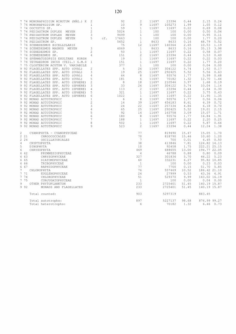
7 74 MONORAPHIDIUM MINUTUM (NÄG.) K 2 92 2 11697 23394 0.44 2.15 0.247 74 MONORAPHIDIUM SP. 1 10 9 11697 105273 1.99 1.05 0.127 74 OOCYSTIS SP. 1 59 1 11697 11697 0.22 0.69 0.087 74 PEDIASTRUM DUPLEX MEYEN 2 5024 1 100 100 0.00 0.50 0.067 74 PEDIASTRUM DUPLEX MEYEN 3 9499 1 100 100 0.00 0.95 0.117 74 PEDIASTRUM DUPLEX MEYEN 5 cf. 17663 1 100 100 0.00 1.77 0.207 74 PEDIASTRUM SP. 5652 1 8633 8633 0.16 48.79 5.527 74 SCENEDESMUS BICELLULARIS 75 12 11697 140364 2.65 10.53 1.197 74 SCENEDESMUS MAGNUS MEYEN 3 4069 1 8633 8633 0.16 35.13 3.987 74 SCENEDESMUS SP. 2 50 1 11697 11697 0.22 0.58 0.077 74 SCENEDESMUS SP. 4 151 2 11697 23394 0.44 3.53 0.407 74 SPERMATOZOPSIS EXULTANS KORSH 19 1 11697 11697 0.22 0.22 0.037 74 TETRAEDRON INCUS (TEIL.) G.M.S 1 151 1 11697 11697 0.22 1.77 0.207 75 CLOSTERIUM ACUTUM V. VARIABILE 377 1 100 100 0.00 0.04 0.009 92 FLAGELLATES SPP. AUTO (OVAL) 2 5 26 11697 304122 5.74 1.52 0.179 92 FLAGELLATES SPP. AUTO (OVAL) 3 19 25 11697 292425 5.52 5.56 0.639 92 FLAGELLATES SPP. AUTO (OVAL) 4 64 8 11697 93576 1.77 5.99 0.689 92 FLAGELLATES SPP. AUTO (OVAL) 5 181 6 11697 70182 1.32 12.70 1.449 92 FLAGELLATES SPP. AUTO (SPHERE) 2 8 18 11697 210546 3.97 1.68 0.199 92 FLAGELLATES SPP. AUTO (SPHERE) 3 33 26 11697 304122 5.74 10.04 1.149 92 FLAGELLATES SPP. AUTO (SPHERE) 4 113 2 11697 23394 0.44 2.64 0.309 92 FLAGELLATES SPP. AUTO (SPHERE) 5 321 1 11697 11697 0.22 3.75 0.439 92 FLAGELLATES SPP. AUTO (SPHERE) 6 1022 1 11697 11697 0.22 11.95 1.359 92 MONAD AUTOTROPHIC 1 6 8 11697 93576 1.77 0.56 0.069 92 MONAD AUTOTROPHIC 2 14 39 11697 456183 8.61 6.39 0.729 92 MONAD AUTOTROPHIC 3 24 22 11697 257334 4.86 6.18 0.709 92 MONAD AUTOTROPHIC 4 65 25 11697 292425 5.52 19.01 2.159 92 MONAD AUTOTROPHIC 5 92 14 11697 163758 3.09 15.07 1.719 92 MONAD AUTOTROPHIC 6 180 8 11697 93576 1.77 16.84 1.919 92 MONAD AUTOTROPHIC 7 188 1 11697 11697 0.22 2.20 0.259 92 MONAD AUTOTROPHIC 8 502 1 11697 11697 0.22 5.87 0.669 92 MONAD AUTOTROPHIC 9 523 2 11697 23394 0.44 12.24 1.38
2 CYANOPHYTA - CYANOPHYCEAE 77 819490 15.47 15.05 1.702 21 CHROOCOCCALES 70 818790 15.46 10.60 1.202 24 OSCILLATORIALES 7 700 0.01 4.45 0.504 CRYPTOPHYTA 38 413846 7.81 124.82 14.135 DINOPHYTA 10 92458 1.75 222.21 25.156 CHRYSOPHYTA 469 688655 13.00 194.77 22.056 62 PRYMNESIOPHYCEAE 4 46788 0.88 0.80 0.096 63 CHRYSOPHYCEAE 327 301836 5.70 46.22 5.236 65 DIATOMOPHYCEAE 60 332231 6.27 95.82 10.856 66 TRIBOPHYCEAE 1 100 0.00 0.23 0.036 67 RAPHIDOPHYCEAE 77 7700 0.15 51.70 5.857 CHLOROPHYTA 76 557469 10.52 186.42 21.107 71 EUGLENOPHYCEAE 24 27999 0.53 43.36 4.917 74 CHLOROPHYCEAE 51 529370 9.99 143.02 16.197 75 CONJUGATOPHYCEAE 1 100 0.00 0.04 0.009 OTHER PHYTOPLANKTON 233 2725401 51.45 140.19 15.879 92 MONADS AND FLAGELLATES 233 2725401 51.45 140.19 15.87
Total counted: 903 5297319 883.45
Total autotrophs: 897 5227137 98.68 876.99 99.27Total heterotrophs: 6 70182 1.32 6.46 0.73
120

SAMPLE: 7346PLACE: Poosjärvi , N EDATE: 21.5.2014DEPTH: 0.00- 1.00 m
COUNTED BY Lounais-Suomen vesi- ja ympäristötutkimus Oy, SA ON 4/22/2015
CHAMBER VOLUME=3ml, DIAM=26mm
BIOMASS OF PHYTOPLANKTON COUNTED WITH Leica DMI3000 B:404 units in 70 Kenttiä at 788x211 units in 50 Kenttiä at 250x94 units in 1 Pohja at 125x
Species Size A/H Volume Units Coeff. Units/l Units % ww µg/l ww %
2 21 CHROOCOCCALES 4 5 5 49573 247865 1.15 1.24 0.042 21 CHROOCOCCALES 6 9 1 49573 49573 0.23 0.45 0.022 21 CHROOCOCCALES 7 10 3 49573 148719 0.69 1.49 0.052 21 CHROOCOCCALES 11 26 2 49573 99146 0.46 2.58 0.092 21 MERISMOPEDIA SP. 1 1 1 49573 49573 0.23 0.05 0.002 24 OSCILLATORIALES 4 1963 2 333 666 0.00 1.31 0.054 0 CRYPTOMONADALES 6 377 3 49573 148719 0.69 56.07 1.964 0 CRYPTOMONAS SP. 2 754 17 7136 121312 0.56 91.47 3.204 0 CRYPTOMONAS SP. 3 1769 13 7136 92768 0.43 164.11 5.744 0 CRYPTOMONAS SP. 5 4136 3 7136 21408 0.10 88.54 3.104 0 KATABLEPHARIS OVALIS SKUJA 1 HET 92 3 49573 148719 0.69 13.68 0.484 0 RHODOMONAS LACUSTRIS PASCH.&R 2 82 2 49573 99146 0.46 8.13 0.284 0 RHODOMONAS LACUSTRIS PASCH.&R 3 122 9 49573 446157 2.07 54.43 1.905 0 DINOPHYCEAE 2 251 1 49573 49573 0.23 12.44 0.445 0 DINOPHYCEAE 6 4421 1 7136 7136 0.03 31.55 1.105 0 PERIDINIUM BIPES STEIN cf. 72220 1 333 333 0.00 24.05 0.846 61 BICOSOECA SP. HET 67 2 49573 99146 0.46 6.64 0.236 62 CHRYSOCHROMULINA SP. 1 9 1 49573 49573 0.23 0.45 0.026 62 CHRYSOCHROMULINA SP. 2 17 21 49573 1041033 4.83 17.70 0.626 62 CHRYSOCHROMULINA SP. 3 25 8 49573 396584 1.84 9.91 0.356 63 CHRYSIDIASTRUM CATENATUM LAUT 1281 3 7136 21408 0.10 27.42 0.966 63 CHRYSOCOCCUS CORDIFORMIS NAUM 205 1 49573 49573 0.23 10.16 0.366 63 DINOBRYON ACUMINATUM RUTTN. 117 2 7136 14272 0.07 1.67 0.066 63 DINOBRYON BAVARICUM IMH. 226 22 7136 156992 0.73 35.48 1.246 63 DINOBRYON BORGEI LEMM. 16 5 49573 247865 1.15 3.97 0.146 63 DINOBRYON DIVERGENS IMH. 153 1 7136 7136 0.03 1.09 0.046 63 DINOBRYON SUECICUM V. LONGISPI 57 2 49573 99146 0.46 5.65 0.206 63 MALLOMONAS PUNCTIFERA KORSH. 3077 2 7136 14272 0.07 43.91 1.546 63 MALLOMONAS SP. 4 837 1 7136 7136 0.03 5.97 0.216 63 PSEUDOKEPHYRION SP. 151 1 49573 49573 0.23 7.49 0.266 63 PSEUDOPEDINELLA SP. 2 65 6 49573 297438 1.38 19.33 0.686 63 PSEUDOPEDINELLA SP. 4 200 8 49573 396584 1.84 79.32 2.776 63 SPINIFEROMONAS SP. 1 65 2 49573 99146 0.46 6.44 0.236 63 SYNURA SP. 2 1055 2 7136 14272 0.07 15.06 0.536 63 UROGLENA SP. 1 105 119 49573 5899187 27.36 619.41 21.666 65 ASTERIONELLA FORMOSA HASS. 1 540 20 7136 142720 0.66 77.07 2.696 65 AULACOSEIRA AMBIGUA (GRUN.) SI 6 1570 44 333 14652 0.07 23.00 0.806 65 AULACOSEIRA ISLANDICA (O.MÜLL. cf. 3184 31 333 10323 0.05 32.87 1.156 65 AULACOSEIRA SP. 1 236 17 7136 121312 0.56 28.63 1.006 65 AULACOSEIRA TENELLA (NYGAARD) 141 2 49573 99146 0.46 13.98 0.496 65 BACILLARIALES 2 135 49 7136 349664 1.62 47.20 1.656 65 EUPODISCALES 4 135 2 49573 99146 0.46 13.38 0.476 65 EUPODISCALES 7 3140 1 7136 7136 0.03 22.41 0.786 65 NITZSCHIA VERMICULARIS (KÜTZ.) cf. 10080 1 7136 7136 0.03 71.93 2.526 65 RHIZOSOLENIA LONGISETA ZACH. 1 1319 5 7136 35680 0.17 47.06 1.656 66 GONIOCHLORIS SMITHII (BOURR.) 6306 1 7136 7136 0.03 45.00 1.576 67 GONYOSTOMUM SEMEN (EHR.) DIES. 1 cf. 9538 5 333 1665 0.01 15.88 0.566 67 GONYOSTOMUM SEMEN (EHR.) DIES. 2 18652 3 333 999 0.00 18.63 0.656 67 GONYOSTOMUM SP. 1 1444 4 7136 28544 0.13 41.22 1.447 71 EUGLENA SP. 1 3224 1 333 333 0.00 1.07 0.047 71 EUGLENA SP. 2 5828 2 333 666 0.00 3.88 0.147 71 PHACUS PLEURONECTES (O.F.MÜLL. 11304 1 333 333 0.00 3.76 0.137 71 PHACUS SUECICUS LEMM. 4306 1 7136 7136 0.03 30.73 1.077 71 PHACUS TORTUS (LEMM.) SKV. 11137 2 333 666 0.00 7.42 0.267 74 CRUCIGENIELLA SP. 209 1 49573 49573 0.23 10.36 0.367 74 KOLIELLA LONGISETA HIND. 126 1 7136 7136 0.03 0.90 0.037 74 MONOMASTIX SP. 1 31 2 49573 99146 0.46 3.07 0.117 74 MONORAPHIDIUM CONTORTUM (THUR. 1 9 1 49573 49573 0.23 0.45 0.027 74 MONORAPHIDIUM CONTORTUM (THUR. 3 26 44 7136 313984 1.46 8.16 0.297 74 MONORAPHIDIUM DYBOWSKII (WOLOS 2 84 1 49573 49573 0.23 4.16 0.157 74 PEDIASTRUM DUPLEX MEYEN 5 17663 1 333 333 0.00 5.88 0.217 74 PEDIASTRUM DUPLEX V. GRACILLIM 5024 1 333 333 0.00 1.67 0.067 74 SCENEDESMUS SP. 1 25 5 49573 247865 1.15 6.20 0.227 74 SCENEDESMUS SP. 4 151 1 49573 49573 0.23 7.49 0.267 74 VOLVOCALES 3 67 2 49573 99146 0.46 6.64 0.239 92 FLAGELLATES SPP. AUTO (OVAL) 2 5 6 49573 297438 1.38 1.49 0.059 92 FLAGELLATES SPP. AUTO (OVAL) 3 19 25 49573 1239325 5.75 23.55 0.829 92 FLAGELLATES SPP. AUTO (OVAL) 4 64 6 49573 297438 1.38 19.04 0.679 92 FLAGELLATES SPP. AUTO (SPHERE) 2 8 10 49573 495730 2.30 3.97 0.149 92 FLAGELLATES SPP. AUTO (SPHERE) 3 33 33 49573 1635909 7.59 53.98 1.899 92 FLAGELLATES SPP. AUTO (SPHERE) 4 113 23 49573 1140179 5.29 128.84 4.519 92 FLAGELLATES SPP. AUTO (SPHERE) 5 321 24 49573 1189752 5.52 381.91 13.359 92 MONAD AUTOTROPHIC 1 6 5 49573 247865 1.15 1.49 0.059 92 MONAD AUTOTROPHIC 2 14 22 49573 1090606 5.06 15.27 0.539 92 MONAD AUTOTROPHIC 3 24 10 49573 495730 2.30 11.90 0.429 92 MONAD AUTOTROPHIC 4 65 7 49573 347011 1.61 22.56 0.79
121
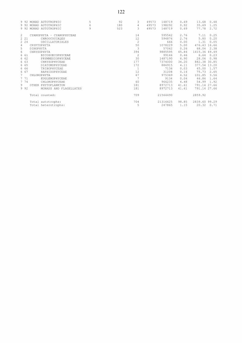
9 92 MONAD AUTOTROPHIC 5 92 3 49573 148719 0.69 13.68 0.489 92 MONAD AUTOTROPHIC 6 180 4 49573 198292 0.92 35.69 1.259 92 MONAD AUTOTROPHIC 9 523 3 49573 148719 0.69 77.78 2.72
2 CYANOPHYTA - CYANOPHYCEAE 14 595542 2.76 7.11 0.252 21 CHROOCOCCALES 12 594876 2.76 5.80 0.202 24 OSCILLATORIALES 2 666 0.00 1.31 0.054 CRYPTOPHYTA 50 1078229 5.00 476.43 16.665 DINOPHYTA 3 57042 0.26 68.04 2.386 CHRYSOPHYTA 394 9885595 45.84 1415.36 49.496 61 BICOSOECOPHYCEAE 2 99146 0.46 6.64 0.236 62 PRYMNESIOPHYCEAE 30 1487190 6.90 28.06 0.986 63 CHRYSOPHYCEAE 177 7374000 34.20 882.38 30.856 65 DIATOMOPHYCEAE 172 886915 4.11 377.54 13.206 66 TRIBOPHYCEAE 1 7136 0.03 45.00 1.576 67 RAPHIDOPHYCEAE 12 31208 0.14 75.73 2.657 CHLOROPHYTA 67 975369 4.52 101.85 3.567 71 EUGLENOPHYCEAE 7 9134 0.04 46.86 1.647 74 CHLOROPHYCEAE 60 966235 4.48 54.99 1.929 OTHER PHYTOPLANKTON 181 8972713 41.61 791.14 27.669 92 MONADS AND FLAGELLATES 181 8972713 41.61 791.14 27.66
Total counted: 709 21564490 2859.92
Total autotrophs: 704 21316625 98.85 2839.60 99.29Total heterotrophs: 5 247865 1.15 20.32 0.71
122

SAMPLE: 14856PLACE: Poosjärvi , N EDATE: 14.8.2014DEPTH: 0.00- 0.00 m
COUNTED BY Lounais-Suomen vesi- ja ympäristötutkimus Oy, SA ON 4/9/2015
CHAMBER VOLUME=3ml, DIAM=26mm
BIOMASS OF PHYTOPLANKTON COUNTED WITH Leica DMI3000 B:532 units in 50 Kenttiä at 788x148 units in 50 Kenttiä at 250x159 units in 1 Pohja at 125x
COMMENT: Lajilistassa nimellä Chrysophyceae 2 olevat solut ovat luultavasti kultaleväkystejä.
Species Size A/H Volume Units Coeff. Units/l Units % ww µg/l ww %
2 21 APHANOCAPSA DELICATISSIMA W.& cf. 88 2 69403 138806 0.37 12.21 0.302 21 APHANOCAPSA SP. 1 16 3 69403 208209 0.55 3.33 0.082 21 APHANOTHECE BACHMANNII KOM.-L 1178 1 69403 69403 0.18 81.76 2.002 21 APHANOTHECE MINUTISSIMA KOM.- 2 68 2 69403 138806 0.37 9.44 0.232 21 APHANOTHECE MINUTISSIMA KOM.- 3 170 1 69403 69403 0.18 11.80 0.292 21 CHROOCOCCALES 4 5 25 69403 1735075 4.59 8.68 0.212 21 CHROOCOCCALES 6 9 1 69403 69403 0.18 0.62 0.022 21 CHROOCOCCALES 7 10 15 69403 1041045 2.75 10.41 0.262 21 CHROOCOCCALES 9 19 2 69403 138806 0.37 2.64 0.062 21 CHROOCOCCALES 11 26 5 69403 347015 0.92 9.02 0.222 21 CHROOCOCCALES 14 47 1 69403 69403 0.18 3.26 0.082 21 CHROOCOCCALES 16 52 1 69403 69403 0.18 3.61 0.092 21 CHROOCOCCALES 18 84 1 69403 69403 0.18 5.83 0.142 21 CHROOCOCCUS SP. 1072 1 69403 69403 0.18 74.40 1.822 21 CYANODICTYON IMPERFECTUM 3 26 22 69403 1526866 4.04 39.70 0.972 21 CYANODICTYON PLANCTONICUM HIC 3 414 2 69403 138806 0.37 57.47 1.412 21 MERISMOPEDIA SP. 1 1 4 69403 277612 0.73 0.28 0.012 21 MERISMOPEDIA SP. 2 11 52 69403 3608956 9.54 39.70 0.972 21 MICROCYSTIS AERUGINOSA (KÜTZ.) 1 6542 1 333 333 0.00 2.18 0.052 21 MICROCYSTIS SP. 5 3271 1 333 333 0.00 1.09 0.032 21 SNOWELLA SP. 3 42 8 69403 555224 1.47 23.32 0.572 21 WORONICHINIA SP. 2 332 1 7136 7136 0.02 2.37 0.064 0 CRYPTOMONADALES 3 94 1 69403 69403 0.18 6.52 0.164 0 CRYPTOMONADALES 4 151 1 69403 69403 0.18 10.48 0.264 0 CRYPTOMONADALES 6 377 1 69403 69403 0.18 26.16 0.644 0 CRYPTOMONAS SP. 2 754 5 7136 35680 0.09 26.90 0.664 0 KATABLEPHARIS OVALIS SKUJA 1 HET 92 2 69403 138806 0.37 12.77 0.314 0 KATABLEPHARIS OVALIS SKUJA 2 HET 170 1 69403 69403 0.18 11.80 0.294 0 RHODOMONAS LACUSTRIS PASCH.&R 2 82 10 69403 694030 1.83 56.91 1.404 0 RHODOMONAS LACUSTRIS PASCH.&R 3 122 1 69403 69403 0.18 8.47 0.215 0 DINOPHYCEAE 4 942 4 7136 28544 0.08 26.89 0.666 62 CHRYSOCHROMULINA SP. 2 17 2 69403 138806 0.37 2.36 0.066 62 CHRYSOCHROMULINA SP. 3 25 1 69403 69403 0.18 1.74 0.046 63 BITRICHIA CHODATII (REV.) CHOD 226 3 7136 21408 0.06 4.84 0.126 63 CHRYSIDIASTRUM CATENATUM LAUT 1281 1 69403 69403 0.18 88.91 2.186 63 CHRYSOPHYCEAE 2 cf. 180 26 69403 1804478 4.77 324.81 7.966 63 DINOBRYON ACUMINATUM RUTTN. 117 7 7136 49952 0.13 5.84 0.146 63 DINOBRYON BAVARICUM IMH. 226 95 333 31635 0.08 7.15 0.186 63 DINOBRYON BORGEI LEMM. 16 2 69403 138806 0.37 2.22 0.056 63 DINOBRYON DIVERGENS IMH. 153 35 333 11655 0.03 1.78 0.046 63 MALLOMONAS PUNCTIFERA KORSH. 3077 1 7136 7136 0.02 21.96 0.546 63 MALLOMONAS SP. 4 837 5 7136 35680 0.09 29.86 0.736 63 PSEUDOPEDINELLA SP. 1 21 1 69403 69403 0.18 1.46 0.046 63 PSEUDOPEDINELLA SP. 2 65 5 69403 347015 0.92 22.56 0.556 63 SPINIFEROMONAS SP. 1 65 1 69403 69403 0.18 4.51 0.116 63 SPINIFEROMONAS SP. 2 180 2 69403 138806 0.37 24.99 0.616 63 UROGLENA SP. 1 105 1 69403 69403 0.18 7.29 0.186 65 ACANTHOCERAS ZACHARIASII (BRUN 13816 2 7136 14272 0.04 197.18 4.836 65 ASTERIONELLA FORMOSA HASS. 1 540 4 7136 28544 0.08 15.41 0.386 65 AULACOSEIRA SP. 1 236 2 7136 14272 0.04 3.37 0.086 65 AULACOSEIRA SP. 2 755 8 7136 57088 0.15 43.10 1.066 65 AULACOSEIRA SP. 3 1570 1 7136 7136 0.02 11.20 0.276 65 AULACOSEIRA TENELLA (NYGAARD) 141 14 69403 971642 2.57 137.00 3.366 65 BACILLARIALES 8 1980 1 7136 7136 0.02 14.13 0.356 65 BACILLARIALES 13 11250 2 333 666 0.00 7.49 0.186 65 BACILLARIALES 15 72000 1 333 333 0.00 23.98 0.596 65 EUPODISCALES 4 135 1 69403 69403 0.18 9.37 0.236 65 FRAGILARIA CONSTRUENS (EHR.) G 1 38 3 69403 208209 0.55 7.91 0.196 65 FRAGILARIA CONSTRUENS (EHR.) G 2 151 25 7136 178400 0.47 26.94 0.666 65 NITZSCHIA SP. 6 49000 1 333 333 0.00 16.32 0.406 65 RHIZOSOLENIA ERIENSIS H.L.SM. 3 612 3 7136 21408 0.06 13.10 0.326 65 RHIZOSOLENIA ERIENSIS H.L.SM. 4 1696 2 7136 14272 0.04 24.21 0.596 65 RHIZOSOLENIA LONGISETA ZACH. 1 1319 3 7136 21408 0.06 28.24 0.696 65 SKELETONEMA POTAMOS (WEBER) H cf. 100 12 7136 85632 0.23 8.56 0.216 65 SYNEDRA ULNA (NITZSCH) EHR. 3 9800 2 333 666 0.00 6.53 0.166 66 CENTRITRACTUS AFRICANUS FRITS cf. 294 3 7136 21408 0.06 6.29 0.156 66 GONIOCHLORIS SP. 1465 1 7136 7136 0.02 10.45 0.266 66 PSEUDOSTAURASTRUM LIMNETICUM ( 1018 1 7136 7136 0.02 7.26 0.186 67 GONYOSTOMUM SEMEN (EHR.) DIES. 2 18652 1 7136 7136 0.02 133.10 3.266 67 GONYOSTOMUM SP. 1 1444 3 7136 21408 0.06 30.91 0.767 71 EUGLENA ACUS EHR. 5652 1 333 333 0.00 1.88 0.057 71 EUGLENA ALLORGEI DEFL. cf. 5613 1 333 333 0.00 1.87 0.057 71 EUGLENA SP. 1 3224 1 7136 7136 0.02 23.01 0.567 71 EUGLENA SPIROGYRA EHR. 2177 1 333 333 0.00 0.72 0.02
123

7 71 PHACUS CURVICAUDA SVIR. 4875 7 333 2331 0.01 11.36 0.287 71 PHACUS LONGICAUDA (EHR.) DUJ. 2 11566 1 333 333 0.00 3.85 0.097 71 PHACUS TORTUS (LEMM.) SKV. 11137 1 333 333 0.00 3.71 0.097 71 TRACHELOMONAS INTERMEDIA DANG 2813 1 7136 7136 0.02 20.07 0.497 73 NEPHROSELMIS OLIVACEA STEIN E 99 1 69403 69403 0.18 6.87 0.177 74 ANKYRA JUDAYI (G.M.SM.) FOTT 71 4 7136 28544 0.08 2.03 0.057 74 BOTRYOCOCCUS SP. 1 589 2 333 666 0.00 0.39 0.017 74 CHLOROCOCCALES 1 8 15 69403 1041045 2.75 8.33 0.207 74 CHLOROCOCCALES 2 24 8 69403 555224 1.47 13.33 0.337 74 CHLOROCOCCALES 3 204 3 69403 208209 0.55 42.47 1.047 74 CRUCIGENIA TETRAPEDIA (KIRCHN. 260 1 69403 69403 0.18 18.04 0.447 74 DICTYOSPHAERIUM PULCHELLUM WO 452 4 69403 277612 0.73 125.48 3.087 74 DICTYOSPHAERIUM SP. 1 18 2 69403 138806 0.37 2.50 0.067 74 ELAKATOTHRIX GENEVENSIS HIND. 1 7 1 69403 69403 0.18 0.49 0.017 74 FRANCEIA SP. 50 1 69403 69403 0.18 3.47 0.097 74 KIRCHNERIELLA CONTORTA (SCHMID 23 14 7136 99904 0.26 2.30 0.067 74 KIRCHNERIELLA SP. 2 100 1 69403 69403 0.18 6.94 0.177 74 KOLIELLA SPIROTAENIA (W. & G. cf. 393 2 333 666 0.00 0.26 0.017 74 MONOMASTIX SP. 1 31 3 69403 208209 0.55 6.45 0.167 74 MONORAPHIDIUM DYBOWSKII (WOLOS 2 84 10 69403 694030 1.83 58.30 1.437 74 MONORAPHIDIUM SP. 1 10 7 69403 485821 1.28 4.86 0.127 74 MONORAPHIDIUM SP. 2 cf. 126 2 7136 14272 0.04 1.80 0.047 74 OOCYSTIS SP. 1 59 2 69403 138806 0.37 8.19 0.207 74 OOCYSTIS SP. 2 196 1 69403 69403 0.18 13.60 0.337 74 PEDIASTRUM ANGULOSUM (EHR.) ME 1 22687 2 333 666 0.00 15.11 0.377 74 PEDIASTRUM DUPLEX MEYEN 3 9499 1 7136 7136 0.02 67.78 1.667 74 PEDIASTRUM DUPLEX V. GRACILLIM 5024 4 7136 28544 0.08 143.41 3.527 74 PEDIASTRUM TETRAS (EHR.) RALFS 2 1809 1 69403 69403 0.18 125.55 3.087 74 PHACOTUS SP. 1 38 1 69403 69403 0.18 2.64 0.067 74 SCENEDESMUS SP. 1 25 21 69403 1457463 3.85 36.44 0.897 74 SCENEDESMUS SP. 2 50 1 69403 69403 0.18 3.47 0.097 74 SCENEDESMUS SP. 3 75 1 69403 69403 0.18 5.21 0.137 74 SCENEDESMUS SP. 4 151 1 69403 69403 0.18 10.48 0.267 74 SCENEDESMUS SP. 5 264 10 7136 71360 0.19 18.84 0.467 74 SCENEDESMUS SP. 6 301 1 69403 69403 0.18 20.89 0.517 74 SCENEDESMUS SUBSPICATUS CHOD. 1 cf. 151 1 69403 69403 0.18 10.48 0.267 74 SIDEROCOELIS SP. cf. 102 1 69403 69403 0.18 7.08 0.177 74 SORASTRUM SP. cf. 3517 2 7136 14272 0.04 50.19 1.237 74 SPERMATOZOPSIS EXULTANS KORSH 19 5 69403 347015 0.92 6.59 0.167 74 TETRAEDRON CAUDATUM (CORDA) HA 1 139 1 69403 69403 0.18 9.65 0.247 74 TETRAEDRON MINIMUM (A.BRAUN) H 256 1 69403 69403 0.18 17.77 0.447 74 TETRASTRUM KOMAREKII HIND. 100 1 69403 69403 0.18 6.94 0.177 74 TETRASTRUM SP. 247 14 69403 971642 2.57 240.00 5.887 74 ULOTRICHALES 1 85 4 69403 277612 0.73 23.60 0.587 74 VOLVOCALES 5 410 1 69403 69403 0.18 28.46 0.707 74 VOLVOCALES 6 904 1 69403 69403 0.18 62.74 1.547 75 CLOSTERIUM ACUTUM V. VARIABILE 377 2 7136 14272 0.04 5.38 0.137 75 CLOSTERIUM PARVULUM NÄG. 3040 1 333 333 0.00 1.01 0.027 75 STAURASTRUM SP. 2 921 2 333 666 0.00 0.61 0.027 75 TEILINGIA GRANULATA (ROY&BISS. 239 9 7136 64224 0.17 15.35 0.389 92 FLAGELLATES SPP. AUTO (OVAL) 2 5 2 69403 138806 0.37 0.69 0.029 92 FLAGELLATES SPP. AUTO (OVAL) 3 19 13 69403 902239 2.39 17.14 0.429 92 FLAGELLATES SPP. AUTO (OVAL) 4 64 8 69403 555224 1.47 35.53 0.879 92 FLAGELLATES SPP. AUTO (OVAL) 5 181 2 69403 138806 0.37 25.12 0.629 92 FLAGELLATES SPP. AUTO (SPHERE) 2 8 6 69403 416418 1.10 3.33 0.089 92 FLAGELLATES SPP. AUTO (SPHERE) 3 33 20 69403 1388060 3.67 45.81 1.129 92 FLAGELLATES SPP. AUTO (SPHERE) 4 113 2 69403 138806 0.37 15.69 0.389 92 FLAGELLATES SPP. AUTO (SPHERE) 5 321 1 69403 69403 0.18 22.28 0.559 92 MONAD AUTOTROPHIC 1 6 4 69403 277612 0.73 1.67 0.049 92 MONAD AUTOTROPHIC 2 14 26 69403 1804478 4.77 25.26 0.629 92 MONAD AUTOTROPHIC 3 24 25 69403 1735075 4.59 41.64 1.029 92 MONAD AUTOTROPHIC 4 65 53 69403 3678359 9.73 239.09 5.869 92 MONAD AUTOTROPHIC 5 92 7 69403 485821 1.28 44.70 1.109 92 MONAD AUTOTROPHIC 6 180 12 69403 832836 2.20 149.91 3.689 92 MONAD AUTOTROPHIC 7 188 1 69403 69403 0.18 13.05 0.329 92 MONAD AUTOTROPHIC 9 523 4 69403 277612 0.73 145.19 3.56
2 CYANOPHYTA - CYANOPHYCEAE 152 10348849 27.36 403.11 9.882 21 CHROOCOCCALES 152 10348849 27.36 403.11 9.884 CRYPTOPHYTA 22 1215531 3.21 160.02 3.925 DINOPHYTA 4 28544 0.08 26.89 0.666 CHRYSOPHYTA 284 4837436 12.79 1334.33 32.716 62 PRYMNESIOPHYCEAE 3 208209 0.55 4.09 0.106 63 CHRYSOPHYCEAE 185 2864183 7.57 548.17 13.446 65 DIATOMOPHYCEAE 87 1700820 4.50 594.04 14.566 66 TRIBOPHYCEAE 5 35680 0.09 24.01 0.596 67 RAPHIDOPHYCEAE 4 28544 0.08 164.01 4.027 CHLOROPHYTA 188 8483944 22.43 1328.23 32.577 71 EUGLENOPHYCEAE 14 18268 0.05 66.48 1.637 73 PRASINOPHYCEAE 1 69403 0.18 6.87 0.177 74 CHLOROPHYCEAE 159 8316778 21.99 1232.53 30.227 75 CONJUGATOPHYCEAE 14 79495 0.21 22.36 0.559 OTHER PHYTOPLANKTON 186 12908958 34.13 826.10 20.259 92 MONADS AND FLAGELLATES 186 12908958 34.13 826.10 20.25
Total counted: 836 37823262 4078.68
Total autotrophs: 833 37615053 99.45 4054.11 99.40Total heterotrophs: 3 208209 0.55 24.57 0.60
124

SAMPLE: 19554PLACE: Poosjärvi , N EDATE: 7.10.2014DEPTH: 0.00- 0.00 m
COUNTED BY Lounais-Suomen vesi- ja ympäristötutkimus Oy, SA ON 4/15/2015
CHAMBER VOLUME=10ml, DIAM=26mm
BIOMASS OF PHYTOPLANKTON COUNTED WITH Leica DMI3000 B:440 units in 75 Kenttiä at 788x102 units in 50 Kenttiä at 250x561 units in 1 Pohja at 125x
COMMENT: Lajilistassa nimellä Chrysophyceae 2 olevat solut ovat luultavasti kultaleväkystejä.
Species Size A/H Volume Units Coeff. Units/l Units % ww µg/l ww %
2 21 CHROOCOCCALES 4 5 4 13881 55524 0.87 0.28 0.032 21 CHROOCOCCALES 6 9 1 13881 13881 0.22 0.12 0.012 21 CHROOCOCCALES 7 10 5 13881 69405 1.09 0.69 0.082 21 CHROOCOCCALES 11 26 6 13881 83286 1.30 2.17 0.252 21 CHROOCOCCALES 16 52 1 13881 13881 0.22 0.72 0.082 21 MERISMOPEDIA SP. 2 11 2 13881 27762 0.43 0.31 0.032 21 ROMERIA SP. 2 13 1 13881 13881 0.22 0.18 0.022 21 SNOWELLA SP. 3 42 1 13881 13881 0.22 0.58 0.074 0 CRYPTOMONADALES 4 151 1 13881 13881 0.22 2.10 0.244 0 CRYPTOMONAS SP. 2 754 25 2141 53525 0.84 40.36 4.614 0 CRYPTOMONAS SP. 3 1769 11 2141 23551 0.37 41.66 4.764 0 CRYPTOMONAS SP. 4 2257 1 2141 2141 0.03 4.83 0.554 0 KATABLEPHARIS OVALIS SKUJA 1 HET 92 5 13881 69405 1.09 6.39 0.734 0 RHODOMONAS LACUSTRIS PASCH.&R 2 82 5 13881 69405 1.09 5.69 0.654 0 RHODOMONAS LACUSTRIS PASCH.&R 3 122 19 13881 263739 4.13 32.18 3.685 0 DINOPHYCEAE 5 2010 1 2141 2141 0.03 4.30 0.495 0 DINOPHYCEAE 7 7235 1 2141 2141 0.03 15.49 1.776 62 CHRYSOCHROMULINA SP. 2 17 4 13881 55524 0.87 0.94 0.116 62 CHRYSOCHROMULINA SP. 3 25 1 13881 13881 0.22 0.35 0.046 63 CHRYSOLYKOS PLANCTONICUS MACK 105 1 13881 13881 0.22 1.46 0.176 63 CHRYSOPHYCEAE 2 180 4 13881 55524 0.87 9.99 1.146 63 DINOBRYON BAVARICUM IMH. 226 76 100 7600 0.12 1.72 0.206 63 DINOBRYON BORGEI LEMM. 16 1 13881 13881 0.22 0.22 0.036 63 DINOBRYON DIVERGENS IMH. 153 450 100 45000 0.71 6.88 0.796 63 DINOBRYON SUECICUM V. LONGISPI 57 1 13881 13881 0.22 0.79 0.096 63 KEPHYRION SP. 92 2 13881 27762 0.43 2.55 0.296 63 MALLOMONAS PUNCTIFERA KORSH. 3077 4 2141 8564 0.13 26.35 3.016 63 MALLOMONAS SP. 3 335 1 13881 13881 0.22 4.65 0.536 63 MALLOMONAS SP. 4 837 2 2141 4282 0.07 3.58 0.416 63 PSEUDOPEDINELLA SP. 2 65 11 13881 152691 2.39 9.92 1.136 63 PSEUDOPEDINELLA SP. 5 471 1 13881 13881 0.22 6.54 0.756 63 SPINIFEROMONAS SP. 1 65 2 13881 27762 0.43 1.80 0.216 63 SYNURA SP. 2 1055 3 13881 41643 0.65 43.93 5.026 63 UROGLENA SP. 1 105 65 13881 902265 14.14 94.74 10.836 65 ASTERIONELLA FORMOSA HASS. 2 1280 8 100 800 0.01 1.02 0.126 65 AULACOSEIRA AMBIGUA (GRUN.) SI 5 904 11 2141 23551 0.37 21.29 2.436 65 AULACOSEIRA SP. 1 236 4 2141 8564 0.13 2.02 0.236 65 AULACOSEIRA SP. 3 1570 1 2141 2141 0.03 3.36 0.386 65 BACILLARIALES 2 135 6 2141 12846 0.20 1.73 0.206 65 BACILLARIALES 8 1980 1 2141 2141 0.03 4.24 0.486 65 BACILLARIALES 12 6075 1 2141 2141 0.03 13.01 1.496 65 EUNOTIA ZASUMINENSIS (CAB.) KÖ 264 16 100 1600 0.03 0.42 0.056 65 EUPODISCALES 5 393 2 13881 27762 0.43 10.91 1.256 65 FRAGILARIA CONSTRUENS (EHR.) G 2 151 5 2141 10705 0.17 1.62 0.186 65 RHIZOSOLENIA LONGISETA ZACH. 1 1319 5 2141 10705 0.17 14.12 1.616 65 RHIZOSOLENIA LONGISETA ZACH. 2 1758 2 2141 4282 0.07 7.53 0.866 65 SYNEDRA ACUS KÜTZ. 4 3200 1 2141 2141 0.03 6.85 0.786 65 SYNEDRA ULNA (NITZSCH) EHR. 3 9800 2 100 200 0.00 1.96 0.226 65 TABELLARIA FLOCCULOSA (ROTH) K 5 3240 6 100 600 0.01 1.94 0.226 67 GONYOSTOMUM SP. 1 1444 5 2141 10705 0.17 15.46 1.777 71 EUGLENOPHYCEAE 1413 1 2141 2141 0.03 3.03 0.357 71 TRACHELOMONAS SP. 2 1592 1 13881 13881 0.22 22.10 2.537 74 CHLOROCOCCALES 2 24 3 13881 41643 0.65 1.00 0.117 74 CHLOROPHYCEAE 1 113 2 13881 27762 0.43 3.14 0.367 74 CRUCIGENIA TETRAPEDIA (KIRCHN. 260 1 13881 13881 0.22 3.61 0.417 74 MONORAPHIDIUM CONTORTUM (THUR. 1 9 4 2141 8564 0.13 0.08 0.017 74 MONORAPHIDIUM CONTORTUM (THUR. 5 59 1 2141 2141 0.03 0.13 0.017 74 MONORAPHIDIUM DYBOWSKII (WOLOS 2 84 1 13881 13881 0.22 1.17 0.137 74 MONORAPHIDIUM GRIFFITHII (BERK 2 141 2 2141 4282 0.07 0.60 0.077 74 MONORAPHIDIUM SP. 1 10 1 13881 13881 0.22 0.14 0.027 74 OOCYSTIS SP. 1 59 1 13881 13881 0.22 0.82 0.097 74 OOCYSTIS SP. 2 196 1 13881 13881 0.22 2.72 0.317 74 PEDIASTRUM BORYANUM (TURP.) ME 20096 1 100 100 0.00 2.01 0.237 74 PEDIASTRUM DUPLEX MEYEN 4 11304 1 100 100 0.00 1.13 0.137 74 PEDIASTRUM TETRAS (EHR.) RALFS 2 1809 1 13881 13881 0.22 25.11 2.877 74 SCENEDESMUS ARMATUS CHOD. 3 402 2 13881 27762 0.43 11.16 1.287 74 SCENEDESMUS COMMUNIS HEGEW. cf. 1099 1 2141 2141 0.03 2.35 0.277 74 SCENEDESMUS SP. 1 25 6 13881 83286 1.30 2.08 0.247 74 SCENEDESMUS SP. 2 50 1 13881 13881 0.22 0.69 0.087 74 SCENEDESMUS SP. 3 75 1 13881 13881 0.22 1.04 0.127 74 SCENEDESMUS SUBSPICATUS CHOD. 2 301 1 13881 13881 0.22 4.18 0.487 74 SPERMATOZOPSIS EXULTANS KORSH cf. 19 1 13881 13881 0.22 0.26 0.037 74 TETRAEDRON SP. 211 1 13881 13881 0.22 2.93 0.337 74 TETRALLANTHOS LAGERHEIMII TEI 3014 1 2141 2141 0.03 6.45 0.74
125

7 74 ULOTRICHALES 1 85 5 2141 10705 0.17 0.91 0.107 74 VOLVOCALES 6 904 1 13881 13881 0.22 12.55 1.437 75 STAURASTRUM AVICULA BREB. 4953 1 100 100 0.00 0.50 0.069 92 FLAGELLATES SPP. AUTO (OVAL) 2 5 4 13881 55524 0.87 0.28 0.039 92 FLAGELLATES SPP. AUTO (OVAL) 3 19 49 13881 680169 10.66 12.92 1.489 92 FLAGELLATES SPP. AUTO (OVAL) 4 64 6 13881 83286 1.30 5.33 0.619 92 FLAGELLATES SPP. AUTO (OVAL) 5 181 5 13881 69405 1.09 12.56 1.449 92 FLAGELLATES SPP. AUTO (SPHERE) 2 8 12 13881 166572 2.61 1.33 0.159 92 FLAGELLATES SPP. AUTO (SPHERE) 3 33 78 13881 1082718 16.96 35.73 4.089 92 FLAGELLATES SPP. AUTO (SPHERE) 4 113 9 13881 124929 1.96 14.12 1.619 92 FLAGELLATES SPP. AUTO (SPHERE) 5 321 3 13881 41643 0.65 13.37 1.539 92 FLAGELLATES SPP. AUTO (SPHERE) 6 1022 1 13881 13881 0.22 14.19 1.629 92 FLAGELLATES SPP. AUTO (SPHERE) 7 2805 2 13881 27762 0.43 77.87 8.909 92 MONAD AUTOTROPHIC 1 6 4 13881 55524 0.87 0.33 0.049 92 MONAD AUTOTROPHIC 2 14 36 13881 499716 7.83 7.00 0.809 92 MONAD AUTOTROPHIC 3 24 14 13881 194334 3.04 4.66 0.539 92 MONAD AUTOTROPHIC 4 65 20 13881 277620 4.35 18.05 2.069 92 MONAD AUTOTROPHIC 5 92 3 13881 41643 0.65 3.83 0.449 92 MONAD AUTOTROPHIC 6 180 15 13881 208215 3.26 37.48 4.289 92 MONAD AUTOTROPHIC 9 523 3 13881 41643 0.65 21.78 2.49
2 CYANOPHYTA - CYANOPHYCEAE 21 291501 4.57 5.05 0.582 21 CHROOCOCCALES 21 291501 4.57 5.05 0.584 CRYPTOPHYTA 67 495647 7.77 133.20 15.235 DINOPHYTA 2 4282 0.07 19.79 2.266 CHRYSOPHYTA 705 1532787 24.02 323.92 37.036 62 PRYMNESIOPHYCEAE 5 69405 1.09 1.29 0.156 63 CHRYSOPHYCEAE 624 1342498 21.04 215.15 24.606 65 DIATOMOPHYCEAE 71 110179 1.73 92.03 10.526 67 RAPHIDOPHYCEAE 5 10705 0.17 15.46 1.777 CHLOROPHYTA 44 393321 6.16 111.88 12.797 71 EUGLENOPHYCEAE 2 16022 0.25 25.12 2.877 74 CHLOROPHYCEAE 41 377199 5.91 86.26 9.867 75 CONJUGATOPHYCEAE 1 100 0.00 0.50 0.069 OTHER PHYTOPLANKTON 264 3664584 57.42 280.83 32.119 92 MONADS AND FLAGELLATES 264 3664584 57.42 280.83 32.11
Total counted: 1103 6382122 874.68
Total autotrophs: 1098 6312717 98.91 868.29 99.27Total heterotrophs: 5 69405 1.09 6.39 0.73
126
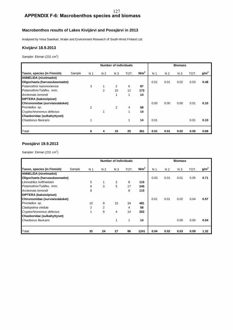
Macrobenthos results of Lakes Kivijärvi and Poosjärvi in 2013
Analysed by Vesa Saarikari, Water and Environment Research of South-West Finland Ltd.
Kivijärvi 18.9.2013
Sampler: Ekman (231 cm2)
Taxon, species (in Finnish) Sample N 1 N 2 N 3 TOT. N/m2N 1 N 2 N 3 TOT. g/m2
ANNELIDA (nivelmadot)
Oligochaeta (harvasukasmadot) 0.01 0.01 0.02 0.03 0.48
Potamothrix hammoniensis 3 1 2 6 87
Potamothrix/Tubifex, imm. 2 10 12 173
Arcteonais lomondi 1 1 14
DIPTERA (kaksisiipiset)
Chironomidae (surviaissääsket) 0.00 0.00 0.00 0.01 0.10
Procladius sp. 2 2 4 58
Cryptochironomus defectus 1 1 14
Chaoboridae (sulkahyttyset)
Chaoborus flavicans 1 1 14 0.01 0.01 0.10
Total: 6 4 15 25 361 0.01 0.01 0.02 0.05 0.68
Poosjärvi 19.9.2013
Sampler: Ekman (231 cm2)
Taxon, species (in Finnish) Sample N 1 N 2 N 3 TOT. N/m2N 1 N 2 N 3 TOT. g/m2
ANNELIDA (nivelmadot)
Oligochaeta (harvasukasmadot) 0.03 0.01 0.01 0.05 0.71
Limnodrilus hoffmeisteri 5 1 2 8 115
Potamothrix/Tubifex, imm. 9 3 5 17 245
Arcteonais lomondi 8 8 115
DIPTERA (kaksisiipiset)
Chironomidae (surviaissääsket) 0.01 0.01 0.02 0.04 0.57
Procladius sp. 10 9 15 34 491
Cladopelma viridula 2 2 4 58
Cryptochironomus defectus 1 9 4 14 202
Chaoboridae (sulkahyttyset)
Chaoborus flavicans 1 1 14 0.00 0.00 0.04
Total: 35 24 27 86 1241 0.04 0.02 0.03 0.09 1.32
Number of individuals Biomass
BiomassNumber of individuals
APPENDIX F-6: Macrobenthos species and biomass127

Macrobenthos results of Lakes Kivijärvi and Poosjärvi in 2014
Analysed by Vesa Saarikari, Water and Environment Research of South-West Finland Ltd.
Kivijärvi 13.10.2014
Sampler: Ekman (231 cm2)
Taxon, species (in Finnish) Sample N 1 N 2 N 3 TOT. N/m2N 1 N 2 N 3 TOT. g/m2
ANNELIDA (nivelmadot)
Oligochaeta (harvasukasmadot) 0.02 0.04 0.01 0.08 1.08
Limnodrilus hoffmeisteri 1 2 3 43
Potamothrix hammoniensis 3 3 43
Potamothrix/Tubifex, imm. 5 7 3 15 216
Ripistes parasita 1 1 14
DIPTERA (kaksisiipiset)
Chironomidae (surviaissääsket) 0.001 0.01 0.00 0.01 0.16
Chironomus plumosus- t. 1 1 14
Procladius sp. 2 3 5 10 144
Cryptochironomus defectus 1 1 14
Tanytarsus sp. 1 1 14
Ceratopogonidae (polttiaiset) 1 1 14 0.01 0.01 0.08
Chaoboridae (sulkahyttyset) 0 0
Chaoborus flavicans 1 1 14 0.004 0.004 0.06
Total: 8 18 11 37 534 0.02 0.05 0.02 0.10 1.38
Poosjärvi 15.10.2014
Sampler: Ekman (231 cm2)
Taxon, species (in Finnish) Sample N 1 N 2 N 3 TOT. N/m2N 1 N 2 N 3 TOT. g/m2
ANNELIDA (nivelmadot)
Oligochaeta (harvasukasmadot) 0.02 0.01 0.02 0.05 0.70
Limnodrilus hoffmeisteri 6 3 5 14 202
Potamothrix hammoniensis 2Potamothrix/Tubifex, imm. 1 2 9 12 173
Pristina foreli 1 1 14
DIPTERA (kaksisiipiset)
Chironomidae (surviaissääsket) 0.01 0.01 0.02 0.04 0.51Procladius sp. 7 14 27 48 693
Cladopelma viridula 1 1 14
Dicrotendipe pulsus 1 1 14
Cladotanytarsus mancus 1 1 14
Ceratopogonidae (polttiaiset) 8 1 9 130 0.01 0.002 0.02 0.24
MOLLUSCA (nilviäiset)
Bivalvia (simpukat) 0.003 0.003 0.04Pisidium sp. 1 1 14
Total: 22 23 44 89 1270 0.04 0.03 0.04 0.10 1.48
BiomassNumber of individuals
BiomassNumber of individuals
128

129
APPENDIX H: Knowledge quality assessment for data
1 Data characteristics
A four-criterion matrix for evaluating data quality is presented in Table 1, and the criteria
can be summarised as:
- Empirical, statistical and methodological quality; from educated guesses to
controlled experiments, direct measurement by best available practise and good
statistical basis;
- Epistemic spatial variability in the scale of the Olkiluoto site, in the assessment
context; from virtually certain to highly unlikely that the parameter value would
significantly differ in other parts of the site for which the underlying data remain
valid;
- Robustness against time scales and external conditions, in the assessment context;
from virtually certain to highly unlikely that the parameter value will be
significantly altered over time or due to changes in the external conditions;
- Appropriateness to the Olkiluoto site in the assessment context; whether the data are
from the site itself or from another site which may be judged on its qualities as an
analogue.
Qualitatively the assessment of data quality can be made by filling to Table 1 the most
appropriate qualitative description of measurements, models and data. If data is rated
other grade than A, then fill "Main assumptions and simplifications" for data also.

130
Table 1. Data quality assessment table (edited from Table 2-2 of POSIVA 2012-28). Criteria for data →
Empirical, statistical and methodological quality
# type of data ↓ A. Directmeasurements /best availablepractise
B. Modelled data /indirect estimates
C. Indirect approximations/ handbook estimates
D. Educatedguesses
1 Element concentrations
x
2 Concentration ratios/Kd values
x
3 Dimensions x 4 Water quality x
Criteria for data →
Epistemic spatial uncertainty to the scale of data (does not include internal (aleatoric) stochastic variation of data)
# type of data ↓ A. Varies unlikely B. Varies possibly C. Varies likely D. Variessignificantlypractically certainly
1 Element concentrations
x
2 Concentration ratios/Kd values
x
3 Dimensions x 4 Water quality x
Criteria for data →
Robustness against assessment time scales and external conditions
# type of data ↓ A. Significantaltering unlikely
B. Significantaltering possible
C. Significant alteringlikely
D. Significantaltering practicallycertain
1 Element concentrations
x
2 Concentration ratios/Kd values
x
3 Dimensions x 4 Water quality x
Criteria for data →
Appropriateness for the assessment context
# type of data ↓ A. Site/disposalconcept specificdata
B. Data from similar sites/disposalconcepts
C. Data possiblyapplicable
D. Data fromelsewhere /applicability notassumable
1 Element concentrations
x
2 Concentration ratios/Kd values
x
3 Dimensions x 4 Water quality x

131
2 Main assumptions
The main assumptions are to be categorized with following list (Data Basis Table 2-1,
below) and described shortly in Table 3.
Table 2. Classification system of assumptions for data, modified from (Nagra 2002)
(Table 2-1 of POSIVA 2012-28). Categorisation of assumptions
LE Conceptual assumption corresponds to the likely/expected characteristics and evolution of the system.
PCA Pessimistic conceptual assumption within the reasonably expected range of possibilities.
WRP Within the range of possibilities but likelihood not currently possible to evaluate — other (and sometimes more pessimistic) assumptions may not be unreasonable.
ST Stylised conceptualisation of system characteristics and evolution.
Table 3. Main assumptions for data. The categorisation of the assumption types is
presented in Table 2. Assumption Category Comment
Concentration ratio approach LE Concentrations are in equilibrium with surrounding media
3 Main uncertainties
The main uncertainties of data are described in Table 4 with causes and effects.
Table 4. Main data uncertainties.
Uncertainty Cause of the uncertainty Effect on the assessment Means to deal with the uncertainty
The quantity that contains the uncertainty
No data available Information density Aleatoric variation Lack of knowledge
Describe the relevance to assessment results
How uncertainty has been taken into account in this report and further work
Concentrations below the limit of quantification
No data available Increases conservativeness in the concentration ratios
Conservative approximation to use quantification limit for the media and half of the quantification limit for the surrounding media.
Number of individuals of some (fish) samples was relatively low
Information density Decreases reliability of the results Comparison with previous results and litterature
4 Overall judgement
Site-specific data is achieved by careful sampling and accredited, standardized analysis
methods. The main uncertainty is caused by concentrations below the limit of
quantification and low number of some samples, especially fish samples.

Wo
rk
ing
Re
po
rt 2
01
4-4
4 •
Re
su
lts o
f Mo
nito
ring
at O
lkilu
oto
in 2
01
3 - H
yd
rog
eo
ch
em
istry


![Digital City, Smart City and Beyond - Amazon Web Servicespapers. · [3] Risto Linturi, Marja-Riitta Koivunen and Jari Sulkanen. Helsinki Arena 2000 - Augmenting a real city to a virtual](https://static.fdocuments.us/doc/165x107/602e03b001dabb1312211352/digital-city-smart-city-and-beyond-amazon-web-3-risto-linturi-marja-riitta.jpg)