Studies on Deformation of Fuchsian Systems from the Title ...

RIGHT:

URL:

CITATION:

AUTHOR(S):

ISSUE DATE:

TITLE:

Studies on Deformation of Fuchsian Systemsfrom the Viewpoint of Rigidity (AlgebraicAnalysis and the Exact WKB Analysis forSystems of Differential Equations)

HARAOKA, Yoshishige

HARAOKA, Yoshishige. Studies on Deformation of Fuchsian Systems from the Viewpoint of Rigidity (Algebraic Analysisand the Exact WKB Analysis for Systems of Differential Equations). 数理解析研究所講究録別冊 2008, B5: 51-60

2008-01

http://hdl.handle.net/2433/174202

RIMS Kôkyûroku BessatsuB5 (2008), 5160

Studies on Deformation of Fuchsian Systemsfrom the Viewpoint of Rigidity

By

Yoshishige Haraoka *

§1. Introduction

We consider a Fuchsian system of differential equations

(1) \displaystyle \frac{dY}{d_{X}}=A(x)Y,where A(x)\in M(n, n;\mathrm{C} Monodromy preserving deformation of (1) is a problemof determining the coefficient matrix A(x) so that the monodromy of (1) does not

change when the positions of the singular points are varied. The deformation equationbecomes a system of differential equations for accessory parameters as functions in the

positions of singular points. When the system (1) is free of accessory parameters, the

deformation equation becomes trivial and is not interesting; however, in this case we can

know many global properties of (1) — the monodromy group, connection coefficients,

integral representations of the solutions, etc. In this sense systems free of accessory

parameters are interesting, and have been studied for a long time.

Recently there are two remarkable progresses in the study of accessory parameter

free systems. One is the work of Katz [14] on rigid local systems, and the other is the

work of Yokoyama [18], [8], both of which give algorithms to construct every systemfree of accessory parameters. The operations in these algorithms can be applied also to

systems containing accessory parameters, which will shed a new light to the deformation

theory. Moreover the notion of rigidity in the Katz theory will give a useful viewpointfor the study of the deformation theory and the theory of holonomic systems.

In this paper we report two results; one is on a relation among the deformation

theory and the rigidity argument, and the other is on a relation among the theory of

Received March 20, 2007, Accepted October 17, 2007.

2000 Mathematics Subject Classification(s): 34\mathrm{M}55, 33\mathrm{C}65.

Supported by the JSPS grant‐in‐aid for scientific research \mathrm{B},

No. 17340049.*

Department of Mathematics, Kumamoto University, Kumamoto 860‐8555, Japan.

© 2008 Research Institute for Mathematical Sciences, Kyoto University. All rights reserved.

52 Yoshishige Haraoka

holonomic systems and the rigidity argument. We also give some problems concerningthe rigidity argument, which seem to be interesting.

§2. Katz Theory and Deformation Theory

Let t_{1}, t_{2} ,. . .

, t_{p} be distinct points in \mathrm{C},and A_{1}, A_{2} ,

. . .

, A_{p}n\times n‐matrices which are

independent of the variable x . We consider a Fuchsian system of differential equations

(2) \displaystyle \frac{dY}{dx}=(\sum_{j=1}^{p}\frac{A_{j}}{x-t_{j}})Y.Note that generically Fuchsian systems (1) can be transformed into a system of the form

(2). The system (2) has regular singular points at x=t_{1}, t_{2} ,. . .

, t_{p}, \infty,

and the residue

matrix at x=\infty is

A_{p+1}:=-\displaystyle \sum_{j=1}^{p}A_{j}.Throughout this paper we assume

(A) for each j ,there is no integral difference among distinct eigenvalues of A_{j}(j=

1,

. . .

, p+1) .

Definition 2.1. A tuple \mathcal{A}=(A\mathrm{l}, . . . , A_{p}, A_{p+1}) of n\times n‐matrices with A_{1}+. . . +A_{p}+A_{p+1}=O is said to be rigid if it is determined by their Jordan canonical

forms C_{1} ,. . .

, C_{p}, C_{p+1} uniquely up to isomorphisms. In other words, a tuple \mathcal{A} is rigid

if, for any tuple \mathcal{B}=(B\mathrm{l}, . . . , B_{p}, B_{p+1}) with B_{1}+\cdots+B_{p}+B_{p+1}=O satisfying

B_{j}=D_{j}A_{j}D_{j}^{-1} with some non‐singular matrix D_{j} for j=1 ,. . .

, p+1 ,there exists a

non‐singular matrix D such that B_{j}=DA_{j}D^{-1} for j=1 ,. . .

, p+1.

The index of rigidity $\iota$ is defined for a tuple \mathcal{A}=(A_{1}, \ldots, A_{p}, A_{p+1}) by

$\iota$=(2-(p+1))n^{2}+\displaystyle \sum_{j=1}^{p+1}\dim Z(A_{j}) ,

where Z() denotes the centralizer of A.

Theorem 2.2 ([14]). If a tuple \mathcal{A} is irreducible, then we have $\iota$\leq 2 . In this

case the tuple \mathcal{A} is rigid if and only if $\iota$=2.

The number 2- $\iota$ can be regarded as the number of the accessory parameters of the

corresponding system (2), and hence the number of the unknowns of the deformation

equation.

Deformation 0F Fuchsian Systems 53

Now we explain the Katz algorithm for constructing rigid tuples. Since a tuple

\mathcal{A}=(A\mathrm{l}, . . . , A_{p}, A_{p+1}) with A_{1}+\cdots+A_{p}+A_{p+1}=O is determined by the first p

matrices (Al, . . .

, A_{p} ), we often use (Al, . . .

, A_{p} ) instead of (Al, . . .

, A_{p}, A_{p+1} ).The Katz algorithm consists of two operations — addition and middle convolution.

For $\alpha$_{j}\in \mathrm{C}(1\leq j\leq p) ,the addition with parameters ($\alpha$_{1}, \ldots, $\alpha$_{p}) is defined by

(Al, . . .

, A_{p} ) \mapsto(A_{1}+$\alpha$_{1}, \ldots, A_{p}+$\alpha$_{p}) .

For $\lambda$\in \mathrm{C} ,the convolution with parameter $\lambda$ is defined by

(Al, . . .

, A_{p} ) \mapsto(G_{1}, \ldots, G_{p}) ,

where G_{j} is a pn\times pn‐matrix given by

G_{j}=j)(A_{1} . . .

for 1\leq j\leq p . We set

A_{j_{O^{+}}^{O}} $\lambda$ . . . A_{p})

\mathcal{K}=\left(\begin{array}{ll}\mathrm{K}\mathrm{e}\mathrm{r} & A_{1}\\\vdots & \\\mathrm{K}\mathrm{e}\mathrm{r} & A_{p}\end{array}\right), \mathcal{L}=\mathrm{K}\mathrm{e}\mathrm{r}(G_{1}+\cdots+G_{p}) .

Then it is easy to see that \mathcal{K} and \mathcal{L} become invariant subspaces for the Gj�s. Thus

we can define \overline{G}_{j} as the action of G_{j} on the quotient space \mathrm{C}^{pn}/(\mathcal{K}+\mathcal{L}) . The middle

convolution with parameter $\lambda$ is defined by

(Al, . . .

, A_{p} ) \mapsto(\overline{G}_{1}, \ldots, \overline{G}_{p}) ,

These definitions are interpretations from the original ones due to Dettweiler and Reiter

[3].

Theorem 2.3 ([14], [3]). The addition and the middle convolution do not changethe index of rigidity.

The addition and the middle convolution can be regarded as operations for a Fuch‐

sian system (2). The addition with parameters ($\alpha$_{1}, \ldots, $\alpha$_{p}) gives the Fuchsian system

(3) \displaystyle \frac{dZ}{dx}=(\sum_{j=1}^{p}\frac{A_{j}+$\alpha$_{j}}{x-t_{j}})Z,


and the middle convolution with parameter $\lambda$ gives

(4) \displaystyle \frac{dW}{dx}=(\sum_{j=1}^{p}\frac{\overline{G}_{j}}{x-t_{j}})W.It is immediate to see that the solutions of (2) and (3) are related as

Z(x)=Y(x)\displaystyle \prod_{j=1}^{p}(x-t_{j})^{$\alpha$_{j}}.It is known ([4]) that the solutions of the system (4) can be obtained as Riemann‐

Liouville transformation of the solutions of (2).We say that the Fuchsian system (2) is rigid if the tuple (Al, . . .

, A_{p}, A_{p+1} ) of

residue matrices is rigid.

Theorem 2.4 ([14], [3]). Any irreducible rigid Fuchsian system can be obtained

from a rank one Fuchsian system by a finite iteration of additions and middle convolu‐

tions.

The monodromy preserving deformation of (2) is described by the Schlesinger sys‐

tem ([16]). Precisely speaking, we have

Theorem 2.5. There exists a fundamental matrix solution Y_{0}(x) of (2) such

that the monodromy matrices with respect to Y_{0}() are independent of t_{1} ,. . .

, t_{p} , ifand only if the Jordan canonical forms of the A_{j} �s are independent of t_{1} ,

. . .

, t_{p} for

1\leq j\leq p+1 and there exists a non‐singular matrix P independent of x such that the

matrices A_{j}'=PA_{j}P^{-1} satisfy

(5) \left\{\begin{array}{l}\frac{\partial A_{i}'}{\partial t_{i}}=-\sum_{k\neq i}\frac{[A_{i}',A_{k}']}{t_{i}-t_{k}},\\\frac{\partial A_{j}'}{\partial t_{i}}=\frac{[A_{i}',A_{j}']}{t_{i}-t_{j}} (j\neq i) .\end{array}\right.The system (5) can be regarded as a system of differential equations for the entries

of the Aj�s, and we denote it by (S). Let C_{j} be a Jordan canonical form which is

independent of t_{1} ,. . .

, t_{p}(1\leq j\leq p+1) . We denote the condition

A_{j}\sim C_{j} (1\leq j\leq p+1)

by (J). Thus the monodromy preserving deformation is described by two conditions (S)and (J).

As is easily seen, the entries of the residue matrices of the systems (3) and (4)are functions of the entries of the Aj�s. Then the systems (S) for (3) and (4) become

systems for the entries of the Aj�s. We showed that these (S) coincide with the original

(S) for (2):


Theorem 2.6 ([6]). The system (S) is invariant by the addition and the middle

convolution.

On the other hand the condition (J) changes when we operate the addition or the

middle convolution. Then, thanks to Theorem 2.6, the addition and the middle convo‐

lution give transformations of solutions of the system (S) with distinct parameters. In

this sense these operations give Bäcklund transformations for the deformation equation.For example, Okamoto�s birational transformation for Painlevé VI is obtained by the

middle convolution ([5], [6]).Painlevé VI is obtained as a deformation equation of the system of rank 2

(6) \displaystyle \frac{dY}{dx}=(\frac{A_{0}}{x}+\frac{A_{1}}{x-1}+\frac{A_{2}}{x-t})Ywhere ([10])

A_{j}=(\displaystyle \frac{z_{j}^{j}+$\theta$_{j}^{j}z+ $\theta$}{u_{j}}--u_{j}z_{j}z_{j}) (j=0,1,2) ,

-(A_{0}+A_{1}+A_{2})=\left(\begin{array}{ll}$\kappa$_{1} & 0\\0 & $\kappa$_{2}\end{array}\right)Also in the works of Boalch [1], Harnad [9] and Mazzocco [15], Painlevé VI appears as

a deformation equation of systems of rank 3. We can see that these systems correspondto the system of rank 3 obtained from (6) by operating a middle convolution.

§3. Rigidity of Appell�s F_{4}

Appell�s hypergeometric series F_{4} is a power series in two variables

F_{4}( $\alpha$, $\beta$, $\gamma,\ \gamma$';x, y)=\displaystyle \sum_{m,n=0}^{\infty}\frac{( $\alpha$,m+n)( $\beta$,m+n)}{( $\gamma$,m)( $\gamma$,n)m!n!}x^{m}y^{n},where $\alpha$, $\beta$, $\gamma$, $\gamma$' are complex parameters satisfying $\gamma$, $\gamma$'\not\in \mathrm{Z}_{\leq 0} ,

and

( $\alpha$, m)=\displaystyle \frac{ $\Gamma$( $\alpha$+m)}{ $\Gamma$( $\alpha$)}.It satisfies a Pfaffian system

(7) dZ= $\Omega$ Z, $\Omega$=A(x, y)dx+B(x, y)dy

of rank 4, where A(x, y) and B(x, y) are rational functions in x, y (the entries of the

unknown vector Z are F_{4} and its partial derivatives). The singular locus of (7) is

L:=\{x=0\}\cup\{y=0\}\cup C\cup\{\infty\},


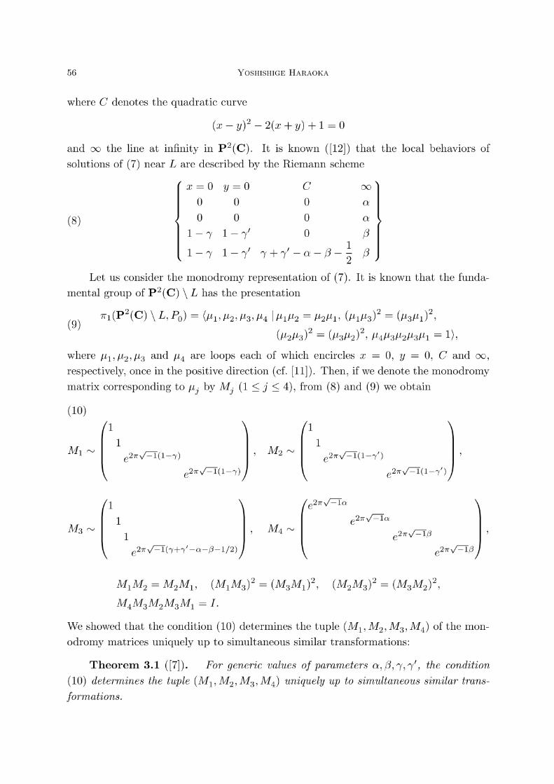
where C denotes the quadratic curve

(x-y)^{2}-2(x+y)+1=0

and \infty the line at infinity in \mathrm{P}^{2}(\mathrm{C}) . It is known ([12]) that the local behaviors of

solutions of (7) near L are described by the Riemann scheme

(8) \left\{\begin{array}{llllll}x & =0 & y & =0 & C & \infty\\ & 0 & & 0 & 0 & $\alpha$\\ & 0 & & 0 & 0 & $\alpha$\\ & 1- $\gamma$ & & $\gamma$ 1- & 0 & $\beta$\\ & 1- $\gamma$ & & $\gamma$'1- & $\gamma$+$\gamma$'- $\alpha$- $\beta$-\frac{1}{2} & $\beta$\end{array}\right\}Let us consider the monodromy representation of (7). It is known that the funda‐

mental group of \mathrm{P}^{2}(\mathrm{C})\backslash L has the presentation

$\pi$_{1}(\mathrm{P}^{2}(\mathrm{C})\backslash L, P_{0})=\langle$\mu$_{1}, $\mu$_{2}, $\mu$_{3}, $\mu$_{4}|$\mu$_{1}$\mu$_{2}=$\mu$_{2}$\mu$_{1}, ($\mu$_{1}$\mu$_{3})^{2}=($\mu$_{3}$\mu$_{1})^{2},(9)

($\mu$_{2}$\mu$_{3})^{2}=($\mu$_{3}$\mu$_{2})^{2}, $\mu$_{4}$\mu$_{3}$\mu$_{2}$\mu$_{3}$\mu$_{1}=1\rangle,where $\mu$_{1}, $\mu$_{2}, $\mu$_{3} and $\mu$_{4} are loops each of which encircles x=0, y=0, C and \infty,

respectively, once in the positive direction (cf. [11]). Then, if we denote the monodromymatrix corresponding to $\mu$_{j} by M_{j}(1\leq j\leq 4) ,

from (8) and (9) we obtain

(10)

M_{1}\sim\left(1 & 1 & e^{2 $\pi$\sqrt{-1}(1- $\gamma$)} & e^{2 $\pi$\sqrt{-1}(1- $\gamma$)}\right), M_{2}\sim\left(1 & 1 & e^{2 $\pi$\sqrt{-1}(1-$\gamma$')} & e^{2 $\pi$\sqrt{-1}(1-$\gamma$')}\right),M_{3}\sim\left(1 & 1 & 1 & e^{2 $\pi$\sqrt{-1}( $\gamma$+$\gamma$'- $\alpha$- $\beta$-1/2)}\right), M_{4}\sim\left(e^{2 $\pi$\sqrt{-1} $\alpha$} & e^{2 $\pi$\sqrt{-1} $\alpha$} & e^{2 $\pi$\sqrt{-1} $\beta$} & e^{2 $\pi$\sqrt{-1} $\beta$}\right),

M_{1}M_{2}=M_{2}M_{1}, (M_{1}M_{3})^{2}=(M_{3}M_{1})^{2}, (M_{2}M_{3})^{2}=(M_{3}M_{2})^{2},

M_{4}M_{3}M_{2}M_{3}M_{1}=I.

We showed that the condition (10) determines the tuple (M_{1}, M_{2}, M_{3}, M_{4}) of the mon‐

odromy matrices uniquely up to simultaneous similar transformations:

Theorem 3.1 ([7]). For generic values of parameters $\alpha$, $\beta$, $\gamma$, $\gamma$' , the condition

(10) determines the tuple (M_{1}, M_{2}, M_{3}, M_{4}) uniquely up to simultaneous similar trans‐

formations.


The result above tells that the monodromy representation of the system (7) defines

a physically rigid local system on \mathrm{P}^{2}(\mathrm{C})\backslash L.It is interesting to compare this result with rigidities of sections of the system (7).

If we restrict the system (7) to the line y =constant, we get the system of ordinarydifferential equations in x

(11) \displaystyle \frac{dZ}{dx}=A(x, y)Z.The Riemann scheme of (11) is

(12) \displaystyle \{00 $\gamma$+$\gamma$'- $\alpha$- $\beta$-\frac{5}{2}x=y-2\sqrt{y}+1000 $\gamma$+$\gamma$'- $\alpha$- $\beta$-\frac{5}{2}x=y+_{0}2\sqrt{y}+100 $\beta$^{-$\gamma$'+1}$\alpha$_{- $\gamma$+1}^{X=\infty} $\alpha \beta$,\},from which we obtain the index of rigidity

$\iota$=(-2)\cdot 4^{2}+(2^{2}+2^{2})+(3^{2}+1^{2})+(3^{2}+1^{2})+(1^{2}+1^{2}+1^{2}+1^{2})=0.

This implies that the system (11) is not rigid, and has 2 accessory parameters. In the

last section we will discuss on the deformation of systems corresponding the Riemann

scheme (12).The line y=constant is not generic, since it goes through the intersection point of

two singular lines \{y=0\} and \infty . If we consider the restriction of (7) on a generic line,we get a system with 6 accessory parameters ([7]). Thus the Pfaffian system (7) givesseveral systems with distinct indexes of rigidity.

§4. Problems

Looking at the above results, we notice several natural problems.Theorem 2.6 asserts that the deformation equation is an invariant under the addi‐

tion and the middle convolution. The converse assertion is not known: Are two Fuchsian

systems connected by the additions and the middle convolutions when they have the

same deformation equation? We know the index of rigidity is also an invariant under

the same operations (Theorem 2.3). What is the difference of these invariants? More

precisely, the index of rigidity gives the number of the unknowns of the deformation

equation, so that, if two systems have the same deformation equations, the indexes of

rigidity of the systems necessarily coincide. Do two Fuchsian systems have the same

deformation equation when they have the same index of rigidity? If the answer is af‐

firmative, the deformation equation of any Fuchsian system becomes a Garnier system,


because any index of rigidity is realized by a Fuchsian system of rank 2. This seems in‐

correct, and we�d like to pose the problem: Describe the difference of the two invariants

— the index of rigidity and the deformation equation.A result in Section 3 gives an interesting example to the last problem. The section

(11) of the Pfaffian system (7) on y =constant has the Riemann scheme (12) and the

index of rigidity 0 . Moreover it contains 4 parameters $\alpha$, $\beta$, $\gamma$, $\gamma$' . On the other hand,the system (6) which yields Painlevé VI has also the index of rigidity 0 and contains 4

parameters $\theta$_{0}, $\theta$_{1}, $\theta$_{2}, $\kappa$_{1} . Note that $\kappa$_{2} is determined by the relation $\theta$_{0}+$\theta$_{1}+$\theta$_{2}+$\kappa$_{1}+$\kappa$_{2}=0 . The former system is of rank 4, while the latter is of rank 2; however, we can operate

the addition and the middle convolution to the latter to obtain the rank 4 system

(13) \displaystyle \frac{dY}{dx}=(\frac{B_{0}}{x}+\frac{B_{1}}{x-1}+\frac{B_{2}}{x-t})Ywith the same deformation equation thanks to Theorem 2.6. The Riemann scheme of

(13) is

(14) \left\{\begin{array}{llll}x=0 & x=1 & x=t & x=\infty\\ 0 & 0 & 0 & - $\lambda$\\ 0 & 0 & 0 & - $\lambda$\\ $\alpha$_{0}+ $\lambda$ & 0 & 0 & $\kappa$_{1}-$\alpha$_{0}- $\lambda$\\ $\theta$_{0}+$\alpha$_{0}+ $\lambda$ & $\theta$_{1}+ $\lambda$ & $\theta$_{2}+ $\lambda$ & $\kappa$_{2}-$\alpha$_{0}- $\lambda$\end{array}\right\}The index of rigidity are calculated by the spectral types of residue matrices. For the

Riemann scheme (12), the spectral types are

(2,2), (3,1), (3,1), (1,1,1,1),

and for (14),(2,1,1), (3,1), (3,1), (2,1,1).

Thus the types are different, while both give the same index of rigidity. Are these

systems connected by the additions and the middle convolutions? A finer invariant may

be given by using the spectral types of residue matrices. This will be a fundamental

problem for the deformation theory and the theory of Fuchsian systems.

We have not yet treated Yokoyama�s algorithm. Similar problems will be posed for

this algorithm. It is also interesting to study the difference of Katz� one and Yokoyama�sone. The difference will appear in constructing non‐rigid Fuchsian systems.

Theorem 3.1 asserts the rigidity of the monodromy representation of the Pfaffian

system (7). However, it seems that the notion of rigidity for local systems over \mathrm{P}^{n}(\mathrm{C})\backslash S,S being a hypersurface, has not yet been established in general. The point for the


definition will be the definition of local monodromies. In particular, if an irreducible

divisor of S has a singularity, it is not clear whether we can define the local monodromyfor the divisor. Zariski�s example [19, Section 8] may explain the difficulty.

We can regard the system (11) as a non‐rigid system which can be prolonged into

a rigid Pfaffian system. The solutions of (11) have integral representation coming from

one for F_{4} ([11], [17]), and we can calculate the monodromy. This suggests us that the

prolongability may correspond to the computability of the monodromy.Another interesting example is given by Kato [13]. He starts from the invariant

polynomials for the complex reflection group G_{336} ,and constructed a linear ordinary

differential equation of the third order whose monodromy group coincides with G_{336}.This system can be prolonged into a Pfaffian system, which turns out to be equivalent to

the system obtained by Boulanger [2]. Also in this case the equation is prolongable and

the monodromy group is computable. Moreover the Pfaffian system thus obtained is so

interesting that it does not come from power series nor integral expression of solutions.

Thus we believe that the rigidity viewpoint will be useful for the study of Fuchsian

systems.

Acknowledgement

The author expresses his sincere gratitude to his collaborators Galina Filipuk and

Youichi Ueno, and to Professors Mitsuo Kato and Joichi Kaneko for their useful sug‐

gestions and the exciting discussions.

References

[1] Boalch, P., From Klein to Painlevé via Fourier, Proc. London Math. Soc. 90 (2005), 167‐

208.

[2] Boulanger, A., Contribution à l�étude des équations différentielles linéaires homogènesintégrables algébriquement, J. Ec. Pol. 4 (1898), 1122.

[3] Dettweiler, M. and Reiter, S., An algorithm of Katz and its application to the inverse

Galois problem, J. Symbolic Comput. 30 (2000), 761798.

[4] Dettweiler, M. and Reiter, S., On the middle convolution, preprint.

[5] Filipuk, G., On the middle convolution and birational symmetries of the sixth Painlevé

equation, Kumamoto J. Math. 19 (2006), 1523.

[6] Haraoka, Y. and Filipuk, G., Middle convolution and deformation for Fuchsian systems,J. London Math. Soc. 76 (2007), 438‐450.

[7] Haraoka, Y. and Ueno, Y., Rigidity for Appell�s hypergeometric series F_{4} ,to appear in

Funkcial. Ekvac.

[8] Haraoka, Y. and Yokoyama, T., Construction of rigid local systems and integral represen‐

tations of their sections, Math. Nachr. 279 (2006), 255271.


[9] Harnad, J., Dual isomonodromic deformations and moment maps to loop algebra, Comm.

Math. Phys. 166 (1994), 337365.

[10] Jimbo, M. and Miwa, T., Monodromy preserving deformations of linear ordinary differ‐

ential equations with rational coefficients II, Physica 2D4 (1981), 407448.

[11] Kaneko, J., Monodromy group of Appell�s system (F4), Tokyo J. Math. 4 (1981), 3554.

[12] Kato, M., The Riemann problem for Appell�s F_{4} ,Mem. Fac. Sci. Kyushu Univ. Ser. A

47 (1993), 227243.

[13] —,Differential equations for invariant curves under Klein�s simple group of order

168, Kyushu J. Math. 58 (2004), 323336.

[14] Katz, N. M., Rigid Local Systems, Princeton Univ. Press, Princeton, NJ, 1996.

[15] Mazzocco, M., Painlevé sixth equation as isomonodromic deformations equation of an

irregular system, The Kowalevski Property (V. B. Kuznetsov, ed CRM Proc. Lecture

Notes 32, Amer. Math. Soc., 2002, pp. 219238.

[16] Schlesinger, L., Über eine Klasse von Differentialsystemen beliebliger Ordnung mit festen

kritischen Punkten, J. für Math. 141 (1912), 96145.

[17] Takano, K., Monodromy group of the system for Appell�s F_{4} ,Funkcial. Ekvac. 23 (1980),

97122.

[18] Yokoyama, T., Construction of systems of differential equations of Okubo normal form

with rigid monodromy, Math. Nachr. 279 (2006), 327348.

[19] Zariski, O., On the problem of existence of algebraic functions of two variables possessinga given branch curve, Amer. J. Math. 51 (1929), 305328.

Studies on Deformation of Fuchsian Systems from the Title ...

Documents

Transcript of Studies on Deformation of Fuchsian Systems from the Title ...