Student Problem Solutions - cin.ufpe.brcin.ufpe.br/~jefl/arquivos/DIP_3E_Student_Solutions.pdf ·...
127
Student Problem Solutions Student Problem Solutions
Transcript of Student Problem Solutions - cin.ufpe.brcin.ufpe.br/~jefl/arquivos/DIP_3E_Student_Solutions.pdf ·...

Student
Problem
Solutions
Student
Problem
Solutions

NOTICE This manual is intended for your personal use only. Copying, printing, posting, or any form of printed or electronic distribution of any part of this manual constitutes a violation of copyright law. As a security measure, this manual was encrypted during download with the serial number of your book, and with your personal information. Any printed or electronic copies of this file will bear that encryption, which will tie the copy to you. Please help us defeat piracy of intellectual property, one of the principal reasons for the increase in the cost of books. -------------------------------


NOTICE This manual is intended for your personal use only. Copying, printing, posting, or any form of printed or electronic distribution of any part of this manual constitutes a violation of copyright law. As a security measure, this manual was encrypted during download with the serial number of your book, and with your personal information. Any printed or electronic copies of this file will bear that encryption, which will tie the copy to you. Please help us defeat piracy of intellectual property, one of the principal reasons for the increase in the cost of books. -------------------------------
Digital Image Processing Third Edition
Student Problem Solutions Version 3.0 Rafael C. Gonzalez Richard E. Woods Prentice Hall Upper Saddle River, NJ 07458 www.imageprocessingplace.com Copyright © 1992-2008 R. C. Gonzalez and R. E. Woods

Chapter 1
Introduction
1.1 About This ManualThis abbreviated manual contains detailed solutions to all problems markedwith a star in Digital Image Processing, 3rd Edition.
1.2 ProjectsYou may be asked by your instructor to prepare comptuter projects in the fol-lowing format:
Page 1: Cover page.
• Project title
• Project number
• Course number
• Student’s name
• Date due
• Date handed in
• Abstract (not to exceed 1/2 page)
Page 2: One to two pages (max) of technical discussion.
Page 3 (or 4): Discussion of results. One to two pages (max).
1

2 CHAPTER 1. INTRODUCTION
Results: Image results (printed typically on a laser or inkjet printer). All imagesmust contain a number and title referred to in the discussion of results.
Appendix: Program listings, focused on any original code prepared by the stu-dent. For brevity, functions and routines provided to the student are referred toby name, but the code is not included.
Layout: The entire report must be on a standard sheet size (e.g., letter size in theU.S. or A4 in Europe), stapled with three or more staples on the left margin toform a booklet, or bound using clear plastic standard binding products.
1.3 About the Book Web SiteThe companion web site
www.prenhall.com/gonzalezwoods
(or its mirror site)
www.imageprocessingplace.com
is a valuable teaching aid, in the sense that it includes material that previouslywas covered in class. In particular, the review material on probability, matri-ces, vectors, and linear systems, was prepared using the same notation as inthe book, and is focused on areas that are directly relevant to discussions in thetext. This allows the instructor to assign the material as independent reading,and spend no more than one total lecture period reviewing those subjects. An-other major feature is the set of solutions to problems marked with a star in thebook. These solutions are quite detailed, and were prepared with the idea ofusing them as teaching support. The on-line availability of projects and digitalimages frees the instructor from having to prepare experiments, data, and hand-outs for students. The fact that most of the images in the book are available fordownloading further enhances the value of the web site as a teaching resource.

NOTICE This manual is intended for your personal use only. Copying, printing, posting, or any form of printed or electronic distribution of any part of this manual constitutes a violation of copyright law. As a security measure, this manual was encrypted during download with the serial number of your book, and with your personal information. Any printed or electronic copies of this file will bear that encryption, which will tie the copy to you. Please help us defeat piracy of intellectual property, one of the principal reasons for the increase in the cost of books. -------------------------------

Chapter 2
Problem Solutions
Problem 2.1The diameter, x , of the retinal image corresponding to the dot is obtained fromsimilar triangles, as shown in Fig. P2.1. That is,
(d /2)0.2
=(x/2)0.017
which gives x = 0.085d . From the discussion in Section 2.1.1, and taking someliberties of interpretation, we can think of the fovea as a square sensor arrayhaving on the order of 337,000 elements, which translates into an array of size580× 580 elements. Assuming equal spacing between elements, this gives 580elements and 579 spaces on a line 1.5 mm long. The size of each element andeach space is then s = [(1.5mm)/1,159] = 1.3× 10⁻⁶ m. If the size (on the fovea)of the imaged dot is less than the size of a single resolution element, we assumethat the dot will be invisible to the eye. In other words, the eye will not detect adot if its diameter, d , is such that 0.085(d )< 1.3× 10⁻⁶ m, or d < 15.3× 10⁻⁶ m.
x/2xImage of the doton the fovea
Edge view of dot
d
d/2
0.2 m 0.017 m
Figure P2.1
3
4 CHAPTER 2. PROBLEM SOLUTIONS
Problem 2.3
The solution is
λ = c/v
= 2.998× 10⁸(m/s)/60(1/s)
= 4.997× 10⁶ m= 4997 Km.
Problem 2.6
One possible solution is to equip a monochrome camera with a mechanical de-vice that sequentially places a red, a green and a blue pass filter in front of thelens. The strongest camera response determines the color. If all three responsesare approximately equal, the object is white. A faster system would utilize threedifferent cameras, each equipped with an individual filter. The analysis thenwould be based on polling the response of each camera. This system would bea little more expensive, but it would be faster and more reliable. Note that bothsolutions assume that the field of view of the camera(s) is such that it is com-pletely filled by a uniform color [i.e., the camera(s) is (are) focused on a part ofthe vehicle where only its color is seen. Otherwise further analysis would be re-quired to isolate the region of uniform color, which is all that is of interest insolving this problem].
Problem 2.9
(a) The total amount of data (including the start and stop bit) in an 8-bit, 1024×1024 image, is (1024)2×[8+2] bits. The total time required to transmit this imageover a 56K baud link is (1024)2× [8+ 2]/56000= 187.25 sec or about 3.1 min.
(b) At 3000K this time goes down to about 3.5 sec.
Problem 2.11
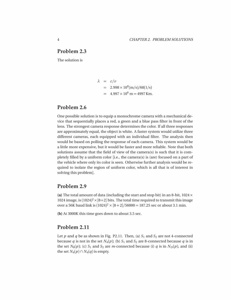
Let p and q be as shown in Fig. P2.11. Then, (a) S1 and S2 are not 4-connectedbecause q is not in the set N4(p ); (b) S1 and S2 are 8-connected because q is inthe set N8(p ); (c) S1 and S2 are m-connected because (i) q is in ND (p ), and (ii)the set N4(p ) ∩N4(q ) is empty.

5
Figure P2.11
Problem 2.12
The solution of this problem consists of defining all possible neighborhood shapesto go from a diagonal segment to a corresponding 4-connected segments as Fig.P2.12 illustrates. The algorithm then simply looks for the appropriate match ev-ery time a diagonal segments is encountered in the boundary.
� or
� or
� or
� or
Figure P2.12
6 CHAPTER 2. PROBLEM SOLUTIONS
Figure P.2.15
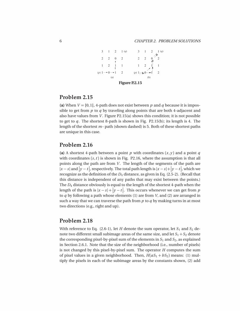
Problem 2.15(a) When V = {0,1}, 4-path does not exist between p and q because it is impos-sible to get from p to q by traveling along points that are both 4-adjacent andalso have values from V . Figure P2.15(a) shows this condition; it is not possibleto get to q . The shortest 8-path is shown in Fig. P2.15(b); its length is 4. Thelength of the shortest m - path (shown dashed) is 5. Both of these shortest pathsare unique in this case.
Problem 2.16(a) A shortest 4-path between a point p with coordinates (x ,y ) and a point qwith coordinates (s , t ) is shown in Fig. P2.16, where the assumption is that allpoints along the path are from V . The length of the segments of the path are|x − s | and
��y − t��, respectively. The total path length is |x − s |+ ��y − t
��, which werecognize as the definition of the D4 distance, as given in Eq. (2.5-2). (Recall thatthis distance is independent of any paths that may exist between the points.)The D4 distance obviously is equal to the length of the shortest 4-path when thelength of the path is |x − s |+ ��y − t
��. This occurs whenever we can get from pto q by following a path whose elements (1) are from V, and (2) are arranged insuch a way that we can traverse the path from p to q by making turns in at mosttwo directions (e.g., right and up).
Problem 2.18With reference to Eq. (2.6-1), let H denote the sum operator, let S1 and S2 de-note two different small subimage areas of the same size, and let S1+S2 denotethe corresponding pixel-by-pixel sum of the elements in S1 and S2, as explainedin Section 2.6.1. Note that the size of the neighborhood (i.e., number of pixels)is not changed by this pixel-by-pixel sum. The operator H computes the sumof pixel values in a given neighborhood. Then, H (aS1 + bS2) means: (1) mul-tiply the pixels in each of the subimage areas by the constants shown, (2) add

7
Figure P2.16
the pixel-by-pixel values from aS1 and bS2 (which produces a single subimagearea), and (3) compute the sum of the values of all the pixels in that single subim-age area. Let a p1 and bp2 denote two arbitrary (but corresponding) pixels fromaS1+bS2. Then we can write
H (aS1+bS2) =∑
p1∈S1 and p2∈S2
a p1+bp2
=∑
p1∈S1
a p1+∑
p2∈S2
bp2
= a∑
p1∈S1
p1+b∑
p2∈S2
p2
= a H (S1)+bH (S2)
which, according to Eq. (2.6-1), indicates that H is a linear operator.
Problem 2.20From Eq. (2.6-5), at any point (x ,y ),
g =1
K
K∑i=1
g i =1
K
K∑i=1
f i +1
K
K∑i=1
ηi .
Then
E {g }= 1
K
K∑i=1
E { f i }+ 1
K
K∑i=1
E {ηi }.But all the f i are the same image, so E { f i } = f . Also, it is given that the noisehas zero mean, so E {ηi } = 0. Thus, it follows that E {g } = f , which proves thevalidity of Eq. (2.6-6).
8 CHAPTER 2. PROBLEM SOLUTIONS
To prove the validity of Eq. (2.6-7) consider the preceding equation again:
g =1
K
K∑i=1
g i =1
K
K∑i=1
f i +1
K
K∑i=1
ηi .
It is known from random-variable theory that the variance of the sum of uncor-related random variables is the sum of the variances of those variables (Papoulis[1991]). Because it is given that the elements of f are constant and the ηi areuncorrelated, then
σ2g =σ
2f +
1
K 2 [σ2η1+σ2
η2+ · · ·+σ2
ηK].
The first term on the right side is 0 because the elements of f are constants. Thevarious σ2
ηiare simply samples of the noise, which is has variance σ2
η. Thus,σ2ηi=σ2
η and we have
σ2g =
K
K 2σ2η =
1
Kσ2η
which proves the validity of Eq. (2.6-7).
Problem 2.22Let g (x ,y ) denote the golden image, and let f (x ,y ) denote any input image ac-quired during routine operation of the system. Change detection via subtrac-tion is based on computing the simple difference d (x ,y ) = g (x ,y )− f (x ,y ). Theresulting image, d (x ,y ), can be used in two fundamental ways for change de-tection. One way is use pixel-by-pixel analysis. In this case we say that f (x ,y ) is“close enough” to the golden image if all the pixels in d (x ,y ) fall within a spec-ified threshold band [Tm i n ,Tm ax ] where Tm i n is negative and Tm ax is positive.Usually, the same value of threshold is used for both negative and positive dif-ferences, so that we have a band [−T,T ] in which all pixels of d (x ,y )must fall inorder for f (x ,y ) to be declared acceptable. The second major approach is sim-ply to sum all the pixels in
��d (x ,y )�� and compare the sum against a threshold Q.
Note that the absolute value needs to be used to avoid errors canceling out. Thisis a much cruder test, so we will concentrate on the first approach.
There are three fundamental factors that need tight control for difference-based inspection to work: (1) proper registration, (2) controlled illumination,and (3) noise levels that are low enough so that difference values are not affectedappreciably by variations due to noise. The first condition basically addressesthe requirement that comparisons be made between corresponding pixels. Twoimages can be identical, but if they are displaced with respect to each other,

9
Figure P2.23
comparing the differences between them makes no sense. Often, special mark-ings are manufactured into the product for mechanical or image-based align-ment
Controlled illumination (note that “illumination” is not limited to visible light)obviously is important because changes in illumination can affect dramaticallythe values in a difference image. One approach used often in conjunction withillumination control is intensity scaling based on actual conditions. For exam-ple, the products could have one or more small patches of a tightly controlledcolor, and the intensity (and perhaps even color) of each pixels in the entire im-age would be modified based on the actual versus expected intensity and/orcolor of the patches in the image being processed.
Finally, the noise content of a difference image needs to be low enough sothat it does not materially affect comparisons between the golden and input im-ages. Good signal strength goes a long way toward reducing the effects of noise.Another (sometimes complementary) approach is to implement image process-ing techniques (e.g., image averaging) to reduce noise.
Obviously there are a number if variations of the basic theme just described.For example, additional intelligence in the form of tests that are more sophisti-cated than pixel-by-pixel threshold comparisons can be implemented. A tech-nique used often in this regard is to subdivide the golden image into differentregions and perform different (usually more than one) tests in each of the re-gions, based on expected region content.
Problem 2.23(a) The answer is shown in Fig. P2.23.

10 CHAPTER 2. PROBLEM SOLUTIONS
Problem 2.26From Eq. (2.6-27) and the definition of separable kernels,
T (u ,v ) =M−1∑x=0
N−1∑y=0
f (x ,y )r (x ,y ,u ,v )
=M−1∑x=0
r1(x ,u )N−1∑y=0
f (x ,y )r2(y ,v )
=M−1∑x=0
T (x ,v )r1(x ,u )
where
T (x ,v ) =N−1∑y=0
f (x ,y )r2(y ,v ).
For a fixed value of x , this equation is recognized as the 1-D transform alongone row of f (x ,y ). By letting x vary from 0 to M −1 we compute the entire arrayT (x ,v ). Then, by substituting this array into the last line of the previous equa-tion we have the 1-D transform along the columns of T (x ,v ). In other words,when a kernel is separable, we can compute the 1-D transform along the rowsof the image. Then we compute the 1-D transform along the columns of this in-termediate result to obtain the final 2-D transform, T (u ,v ). We obtain the sameresult by computing the 1-D transform along the columns of f (x ,y ) followed bythe 1-D transform along the rows of the intermediate result.
This result plays an important role in Chapter 4 when we discuss the 2-DFourier transform. From Eq. (2.6-33), the 2-D Fourier transform is given by
T (u ,v ) =M−1∑x=0
N−1∑y=0
f (x ,y )e−j 2π(u x/M+v y /N ).
It is easily verified that the Fourier transform kernel is separable (Problem 2.25),so we can write this equation as
T (u ,v ) =M−1∑x=0
N−1∑y=0
f (x ,y )e−j 2π(u x/M+v y /N )
=M−1∑x=0
e−j 2π(u x/M )N−1∑y=0
f (x ,y )e−j 2π(v y /N )
=M−1∑x=0
T (x ,v )e−j 2π(u x/M )

11
where
T (x ,v ) =N−1∑y=0
f (x ,y )e−j 2π(v y /N )
is the 1-D Fourier transform along the rows of f (x ,y ), as we let x = 0,1, . . . ,M−1.

NOTICE This manual is intended for your personal use only. Copying, printing, posting, or any form of printed or electronic distribution of any part of this manual constitutes a violation of copyright law. As a security measure, this manual was encrypted during download with the serial number of your book, and with your personal information. Any printed or electronic copies of this file will bear that encryption, which will tie the copy to you. Please help us defeat piracy of intellectual property, one of the principal reasons for the increase in the cost of books. -------------------------------

Chapter 3
Problem Solutions
Problem 3.1Let f denote the original image. First subtract the minimum value of f denotedf min from f to yield a function whose minimum value is 0:
g 1 = f − f min
Next divide g 1 by its maximum value to yield a function in the range [0,1] andmultiply the result by L− 1 to yield a function with values in the range [0, L− 1]
g =L− 1
max�
g 1� g 1
=L− 1
max�
f − f min� � f − f min
�Keep in mind that f min is a scalar and f is an image.
Problem 3.3(a) s = T (r ) = 1
1+(m/r )E .
Problem 3.5(a) The number of pixels having different intensity level values would decrease,thus causing the number of components in the histogram to decrease. Becausethe number of pixels would not change, this would cause the height of some ofthe remaining histogram peaks to increase in general. Typically, less variabilityin intensity level values will reduce contrast.
13
14 CHAPTER 3. PROBLEM SOLUTIONS
L � 1
2( 1)L �
L � 1L/4 3 /4LL/20
L � 1
( 1)/2L �
L � 1
L/4 3 /4LL/20
Figure P3.9.
Problem 3.6All that histogram equalization does is remap histogram components on the in-tensity scale. To obtain a uniform (flat) histogram would require in general thatpixel intensities actually be redistributed so that there are L groups of n/L pixelswith the same intensity, where L is the number of allowed discrete intensity lev-els and n =M N is the total number of pixels in the input image. The histogramequalization method has no provisions for this type of (artificial) intensity redis-tribution process.
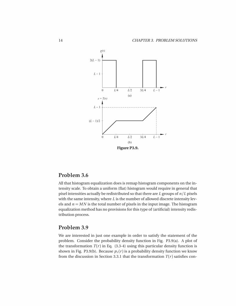
Problem 3.9We are interested in just one example in order to satisfy the statement of theproblem. Consider the probability density function in Fig. P3.9(a). A plot ofthe transformation T (r ) in Eq. (3.3-4) using this particular density function isshown in Fig. P3.9(b). Because pr (r ) is a probability density function we knowfrom the discussion in Section 3.3.1 that the transformation T (r ) satisfies con-

15
ditions (a) and (b) stated in that section. However, we see from Fig. P3.9(b) thatthe inverse transformation from s back to r is not single valued, as there are aninfinite number of possible mappings from s = (L− 1)/2 back to r . It is impor-tant to note that the reason the inverse transformation function turned out notto be single valued is the gap in pr (r ) in the interval [L/4,3L/4].
Problem 3.10
(b) If none of the intensity levels rk , k = 1,2, . . . , L − 1, are 0, then T (rk ) will bestrictly monotonic. This implies a one-to-one mapping both ways, meaning thatboth forward and inverse transformations will be single-valued.
Problem 3.12The value of the histogram component corresponding to the kth intensity levelin a neighborhood is
pr (rk ) =n k
n
for k = 1,2, . . . , K − 1, where n k is the number of pixels having intensity level rk ,n is the total number of pixels in the neighborhood, and K is the total numberof possible intensity levels. Suppose that the neighborhood is moved one pixelto the right (we are assuming rectangular neighborhoods). This deletes the left-most column and introduces a new column on the right. The updated histogramthen becomes
p ′r (rk ) =1
n[n k −n L k +n Rk ]
for k = 0,1, . . . , K − 1, where n L k is the number of occurrences of level rk on theleft column and n Rk is the similar quantity on the right column. The precedingequation can be written also as
p ′r (rk ) = pr (rk )+1
n[n Rk −n L k ]
for k = 0,1, . . . , K −1. The same concept applies to other modes of neighborhoodmotion:
p ′r (rk ) = pr (rk )+1
n[bk −a k ]
for k = 0,1, . . . , K −1, where a k is the number of pixels with value rk in the neigh-borhood area deleted by the move, and bk is the corresponding number intro-duced by the move.

16 CHAPTER 3. PROBLEM SOLUTIONS
Problem 3.13The purpose of this simple problem is to make the student think of the meaningof histograms and arrive at the conclusion that histograms carry no informationabout spatial properties of images. Thus, the only time that the histogram of theimages formed by the operations shown in the problem statement can be de-termined in terms of the original histograms is when one (both) of the imagesis (are) constant. In (d) we have the additional requirement that none of thepixels of g (x , y ) can be 0. Assume for convenience that the histograms are notnormalized, so that, for example, h f (rk ) is the number of pixels in f (x , y ) havingintensity level rk . Assume also that all the pixels in g (x , y ) have constant value c .The pixels of both images are assumed to be positive. Finally, let u k denote theintensity levels of the pixels of the images formed by any of the arithmetic oper-ations given in the problem statement. Under the preceding set of conditions,the histograms are determined as follows:
(a) We obtain the histogram hsum(u k ) of the sum by letting u k = rk + c , and alsohsum(u k ) = h f (rk ) for all k . In other words, the values (height) of the compo-nents of hsum are the same as the components of h f , but their locations on theintensity axis are shifted right by an amount c .
Problem 3.15(a) Consider a 3×3 mask first. Because all the coefficients are 1 (we are ignoringthe 1/9 scale factor), the net effect of the lowpass filter operation is to add all theintensity values of pixels under the mask. Initially, it takes 8 additions to producethe response of the mask. However, when the mask moves one pixel location tothe right, it picks up only one new column. The new response can be computedas
Rnew =Rold−C1+C3
where C1 is the sum of pixels under the first column of the mask before it wasmoved, and C3 is the similar sum in the column it picked up after it moved. Thisis the basic box-filter or moving-average equation. For a 3× 3 mask it takes 2additions to get C3 (C1 was already computed). To this we add one subtractionand one addition to get Rnew. Thus, a total of 4 arithmetic operations are neededto update the response after one move. This is a recursive procedure for movingfrom left to right along one row of the image. When we get to the end of a row, wemove down one pixel (the nature of the computation is the same) and continuethe scan in the opposite direction.
For a mask of size n ×n , (n − 1) additions are needed to obtain C3, plus thesingle subtraction and addition needed to obtain Rnew, which gives a total of

17
(n + 1) arithmetic operations after each move. A brute-force implementationwould require n 2− 1 additions after each move.
Problem 3.16(a) The key to solving this problem is to recognize (1) that the convolution re-sult at any location (x ,y ) consists of centering the mask at that point and thenforming the sum of the products of the mask coefficients with the correspondingpixels in the image; and (2) that convolution of the mask with the entire imageresults in every pixel in the image being visited only once by every element ofthe mask (i.e., every pixel is multiplied once by every coefficient of the mask).Because the coefficients of the mask sum to zero, this means that the sum of theproducts of the coefficients with the same pixel also sum to zero. Carrying outthis argument for every pixel in the image leads to the conclusion that the sumof the elements of the convolution array also sum to zero.
Problem 3.18(a) There are n 2 points in an n × n median filter mask. Because n is odd, themedian value, ζ, is such that there are (n 2− 1)/2 points with values less than orequal to ζ and the same number with values greater than or equal to ζ. How-ever, because the area A (number of points) in the cluster is less than one halfn 2, and A and n are integers, it follows that A is always less than or equal to(n 2 − 1)/2. Thus, even in the extreme case when all cluster points are encom-passed by the filter mask, there are not enough points in the cluster for any ofthem to be equal to the value of the median (remember, we are assuming thatall cluster points are lighter or darker than the background points). Therefore, ifthe center point in the mask is a cluster point, it will be set to the median value,which is a background shade, and thus it will be “eliminated” from the cluster.This conclusion obviously applies to the less extreme case when the number ofcluster points encompassed by the mask is less than the maximum size of thecluster.
Problem 3.19(a) Numerically sort the n 2 values. The median is
ζ= [(n 2+ 1)/2]-th largest value.
(b) Once the values have been sorted one time, we simply delete the values inthe trailing edge of the neighborhood and insert the values in the leading edge

18 CHAPTER 3. PROBLEM SOLUTIONS
Figure P3.21
in the appropriate locations in the sorted array.
Problem 3.21From Fig. 3.33 we know that the vertical bars are 5 pixels wide, 100 pixels high,and their separation is 20 pixels. The phenomenon in question is related to thehorizontal separation between bars, so we can simplify the problem by consid-ering a single scan line through the bars in the image. The key to answering thisquestion lies in the fact that the distance (in pixels) between the onset of one barand the onset of the next one (say, to its right) is 25 pixels.
Consider the scan line shown in Fig. P3.21. Also shown is a cross sectionof a 25× 25 mask. The response of the mask is the average of the pixels that itencompasses. We note that when the mask moves one pixel to the right, it losesone value of the vertical bar on the left, but it picks up an identical one on theright, so the response doesn’t change. In fact, the number of pixels belongingto the vertical bars and contained within the mask does not change, regardlessof where the mask is located (as long as it is contained within the bars, and notnear the edges of the set of bars).
The fact that the number of bar pixels under the mask does not change is dueto the peculiar separation between bars and the width of the lines in relationto the 25-pixel width of the mask This constant response is the reason why nowhite gaps are seen in the image shown in the problem statement. Note that thisconstant response does not happen with the 23×23 or the 45×45 masks becausethey are not ”synchronized” with the width of the bars and their separation.
Problem 3.24The Laplacian operator is defined as
∇2 f =∂ 2 f
∂ x 2+∂ 2 f
∂ y 2

19
for the unrotated coordinates, and as
∇2 f =∂ 2 f
∂ x ′2 +∂ 2 f
∂ y ′2 .
for rotated coordinates. It is given that
x = x ′ cosθ − y ′ sinθ and y = x ′ sinθ + y ′ cosθ
where θ is the angle of rotation. We want to show that the right sides of the first
two equations are equal. We start with
∂ f
∂ x ′ =∂ f
∂ x
∂ x
∂ x ′ +∂ f
∂ y
∂ y
∂ x ′
=∂ f
∂ xcosθ +
∂ f
∂ ysinθ .
Taking the partial derivative of this expression again with respect to x ′ yields
∂ 2 f
∂ x ′2 =∂ 2 f
∂ x 2 cos2θ +∂
∂ x
�∂ f
∂ y
�sinθ cosθ +
∂
∂ y
�∂ f
∂ x
�cosθ sinθ +
∂ 2 f
∂ y 2 sin2θ .
Next, we compute
∂ f
∂ y ′ =∂ f
∂ x
∂ x
∂ y ′ +∂ f
∂ y
∂ y
∂ y ′
=−∂ f
∂ xsinθ +
∂ f
∂ ycosθ .
Taking the derivative of this expression again with respect to y ′ gives
∂ 2 f
∂ y ′2 =∂ 2 f
∂ x 2 sin2θ − ∂∂ x
�∂ f
∂ y
�cosθ sinθ − ∂
∂ y
�∂ f
∂ x
�sinθ cosθ +
∂ 2 f
∂ y 2 cos2θ .
Adding the two expressions for the second derivatives yields
∂ 2 f
∂ x ′2 +∂ 2 f
∂ y ′2 =∂ 2 f
∂ x 2 +∂ 2 f
∂ y 2
which proves that the Laplacian operator is independent of rotation.
20 CHAPTER 3. PROBLEM SOLUTIONS
Problem 3.25The Laplacian mask with a−4 in the center performs an operation proportionalto differentiation in the horizontal and vertical directions. Consider for a mo-ment a 3× 3 “Laplacian” mask with a −2 in the center and 1s above and belowthe center. All other elements are 0. This mask will perform differentiation inonly one direction, and will ignore intensity transitions in the orthogonal direc-tion. An image processed with such a mask will exhibit sharpening in only onedirection. A Laplacian mask with a -4 in the center and 1s in the vertical andhorizontal directions will obviously produce an image with sharpening in bothdirections and in general will appear sharper than with the previous mask. Sim-ilarly, and mask with a −8 in the center and 1s in the horizontal, vertical, anddiagonal directions will detect the same intensity changes as the mask with the−4 in the center but, in addition, it will also be able to detect changes along thediagonals, thus generally producing sharper-looking results.
Problem 3.28Consider the following equation:
f (x ,y )−∇2 f (x ,y ) = f (x ,y )− � f (x + 1,y )+ f (x − 1,y )+ f (x ,y + 1)
+ f (x ,y − 1)− 4f (x ,y )
= 6f (x ,y )− � f (x + 1,y )+ f (x − 1,y )+ f (x ,y + 1)
+ f (x ,y − 1)+ f (x ,y )
= 5
1.2f (x ,y )−1
5
�f (x + 1,y )+ f (x − 1,y )+ f (x ,y + 1)
+ f (x ,y − 1)+ f (x ,y )�
= 5�
1.2f (x ,y )− f (x ,y )
where f (x ,y ) denotes the average of f (x ,y ) in a predefined neighborhood cen-tered at (x ,y ) and including the center pixel and its four immediate neighbors.Treating the constants in the last line of the above equation as proportionalityfactors, we may write
f (x ,y )−∇2 f (x ,y )� f (x ,y )− f (x ,y ).
The right side of this equation is recognized within the just-mentioned propor-tionality factors to be of the same form as the definition of unsharp maskinggiven in Eqs. (3.6-8) and (3.6-9). Thus, it has been demonstrated that subtract-ing the Laplacian from an image is proportional to unsharp masking.

21
Problem 3.33The thickness of the boundaries increases as a the size of the filtering neigh-borhood increases. We support this conclusion with an example. Consider aone-pixel-thick straight black line running vertically through a white image. Ifa 3× 3 neighborhood is used, any neighborhoods whose centers are more thantwo pixels away from the line will produce differences with values of zero and thecenter pixel will be designated a region pixel. Leaving the center pixel at samelocation, if we increase the size of the neighborhood to, say, 5× 5, the line willbe encompassed and not all differences be zero, so the center pixel will now bedesignated a boundary point, thus increasing the thickness of the boundary. Asthe size of the neighborhood increases, we would have to be further and furtherfrom the line before the center point ceases to be called a boundary point. Thatis, the thickness of the boundary detected increases as the size of the neighbor-hood increases.
Problem 3.34(a) If the intensity of the center pixel of a 3× 3 region is larger than the intensityof all its neighbors, then decrease it. If the intensity is smaller than the intensityof all its neighbors, then increase it. Else, do not nothing.
(b) Rules
IF d 2 is PO AND d 4 is PO AND d 6 is PO AND d 8 is PO THEN v is POIF d 2 is NE AND d 4 is NE AND d 6 is NE AND d 8 is NE THEN v is NEELSE v is ZR.
Note: In rule 1, all positive differences mean that the intensity of the noise pulse(z 5) is less than that of all its 4-neighbors. Then we’ll want to make the outputz ′5 more positive so that when it is added to z 5 it will bring the value of the cen-ter pixel closer to the values of its neighbors. The converse is true when all thedifferences are negative. A mixture of positive and negative differences calls forno action because the center pixel is not a clear spike. In this case the correctionshould be zero (keep in mind that zero is a fuzzy set too).

NOTICE This manual is intended for your personal use only. Copying, printing, posting, or any form of printed or electronic distribution of any part of this manual constitutes a violation of copyright law. As a security measure, this manual was encrypted during download with the serial number of your book, and with your personal information. Any printed or electronic copies of this file will bear that encryption, which will tie the copy to you. Please help us defeat piracy of intellectual property, one of the principal reasons for the increase in the cost of books. -------------------------------

Chapter 4
Problem Solutions
Problem 4.2
(a) To prove infinite periodicity in both directions with period 1/ΔT , we have toshow that F
�μ+k [1/ΔT ]
�= F (μ) for k = 0,±1,±2, . . . . From Eq. (4.3-5),
F�μ+k [1/ΔT ]
�=
1
�T
∞∑n=−∞
F
�μ+
k
�T− n
�T
�
=1
�T
∞∑n=−∞
F
�μ+
k −n
�T
�
=1
�T
∞∑m=−∞
F
�μ− m
�T
�
= F�μ�
where the third line follows from the fact that k and n are integers and the limitsof summation are symmetric about the origin. The last step follows from Eq.(4.3-5).
(b) Again, we need to show that F�μ+k/ΔT
�= F (μ) for k = 0,±1,±2, . . . . From
Eq. (4.4-2),
23
24 CHAPTER 4. PROBLEM SOLUTIONS
F�μ+k/ΔT
�=
∞∑n=−∞
f n e−j 2π(μ+k /ΔT )nΔT
=∞∑
n=−∞f n e−j 2πμnΔT e−j 2πk n
=∞∑
n=−∞f n e−j 2πμnΔT
= F�μ�
where the third line follows from the fact that e−j 2πk n = 1 because both k and nare integers (see Euler’s formula), and the last line follows from Eq. (4.4-2).
Problem 4.3From the definition of the 1-D Fourier transform in Eq. (4.2-16),
F�μ�=
∫ ∞−∞
f (t )e−j 2πμt d t
=
∫ ∞−∞
sin (2πnt ) e−j 2πμt d t
=−j
2
∫ ∞−∞
�e j 2πnt − e−j 2πnt
e−j 2πμt d t
=−j
2
∫ ∞−∞
�e j 2πnt
e−j 2πμt d t − −j
2
∫ ∞−∞
�e−j 2πnt
e−j 2πμt d t .
From the translation property in Table 4.3 we know that
f (t )e j 2πμ0t ⇔ F�μ−μ0
�and we know from the statement of the problem that the Fourier transform of aconstant
�f (t ) = 1
is an impulse. Thus,
(1)e j 2πμ0t ⇔δ�μ−μ0
�.
Thus, we see that the leftmost integral in the the last line above is the Fouriertransform of (1)e j 2πnt , which is δ
�μ−n
�, and similarly, the second integral is
the transform of (1) e−j 2πnt , or δ�μ+n
�. Combining all results yields
F�μ�=
j
2
�δ�μ+n
�−δ�μ−n�
as desired.

25
n- n�
F( )�
(a)
n
�n
� T
1
� n� T
1
� T
�1
� T
1+ n
. . . .
. . . .
�
F( )�
(b)
Figure P4.4
Problem 4.4
(a) The period is such that 2πnt = 2π, or t = 1/n .
(b) The frequency is 1 divided by the period, or n . The continuous Fourier trans-form of the given sine wave looks as in Fig. P4.4(a) (see Problem 4.3), and thetransform of the sampled data (showing a few periods) has the general form il-lustrated in Fig. P4.4(b) (the dashed box is an ideal filter that would allow recon-struction if the sine function were sampled, with the sampling theorem beingsatisfied).
(c) The Nyquist sampling rate is exactly twice the highest frequency, or 2n . Thatis, (1/ΔT ) = 2n , or ΔT = 1/2n . Taking samples at t = ±ΔT,±2ΔT, . . . wouldyield the sampled function sin (2πnΔT ) whose values are all 0s because ΔT =1/2n and n is an integer. In terms of Fig. P4.4(b), we see that when ΔT = 1/2nall the positive and negative impulses would coincide, thus canceling each otherand giving a result of 0 for the sampled data.

26 CHAPTER 4. PROBLEM SOLUTIONS
Problem 4.5Starting from Eq. (4.2-20),
f (t ) g (t ) =
∫ ∞−∞
f (τ)g (t −τ)dτ.
The Fourier transform of this expression is
ℑ� f (t ) g (t )=
∫ ∞−∞
⎡⎣∫ ∞−∞
f (τ)g (t −τ)dτ⎤⎦e−j 2πμt d t
=
∫ ∞−∞
f (τ)
⎡⎣∫ ∞−∞
g (t −τ)e−j 2πμt d t
⎤⎦dτ.
The term inside the inner brackets is the Fourier transform of g (t −τ). But, weknow from the translation property (Table 4.3) that
ℑ�g (t −τ)=G (μ)e−j 2πμτ
so
ℑ� f (t ) g (t )=
∫ ∞−∞
f (τ)�
G (μ)e−j 2πμτ
dτ
= G (μ)
∫ ∞−∞
f (τ)e−j 2πμτdτ
= G (μ)F (μ).
This proves that multiplication in the frequency domain is equal to convolutionin the spatial domain. The proof that multiplication in the spatial domain isequal to convolution in the spatial domain is done in a similar way.
Problem 4.8
(b) We solve this problem as above, by direct substitution and using orthogonal-ity. Substituting Eq. (4.4-7) into (4.4-6) yields
F (u ) =M−1∑x=0
⎡⎣ 1
M
M−1∑r=0
F (u )e−j 2πr x/M
⎤⎦e−j 2πu x/M
=1
M
M−1∑r=0
F (r )
⎡⎣M−1∑
x=0
e−j 2πr x/M e−j 2πu x/M
⎤⎦
= F (u )

27
where the last step follows from the orthogonality condition given in the prob-lem statement. Substituting Eq. (4.4-6) into (4.6-7) and using the same basicprocedure yields a similar identity for f (x ).
Problem 4.10With reference to the statement of the convolution theorem given in Eqs. (4.2-21) and (4.2-22), we need to show that
f (x ) h(x )⇔ F (u )H (u )
and thatf (x )h(x )⇔ F (u ) H (u ).
From Eq. (4.4-10) and the definition of the DFT in Eq. (4.4-6),
ℑ� f (x ) h(x )=
M−1∑x=0
⎡⎣M−1∑
m=0
f (m )h(x −m )
⎤⎦e−j 2πu x/M
=M−1∑m=0
f (m )
⎡⎣M−1∑
x=0
h(x −m )e−j 2πu x/M
⎤⎦
=M−1∑m=0
f (m )H (u )e−j 2πu m/M
= H (u )M−1∑m=0
f (m )e−j 2πu m/M
= H (u )F (u ).
The other half of the discrete convolution theorem is proved in a similar manner.
Problem 4.11With reference to Eq. (4.2-20),
f (t ,z ) h(t ,z ) =
∫ ∞−∞
∫ ∞−∞
f (α,β )h(t −α,z −β )dαdβ .
Problem 4.14From Eq. (4.5-7),
Recall that in this chapter weuse (t ,z ) and (μ,ν ) forcontinuous variables, and(x ,y ) and (u ,v ) for discretevariables.
F (μ,ν ) = ℑ� f (t ,z )=
∫ ∞−∞
∫ ∞−∞
f (t ,z )e−j 2π(μt+νz )d t d z .
28 CHAPTER 4. PROBLEM SOLUTIONS
From Eq. (2.6-2), the Fourier transform operation is linear if
ℑ�a 1 f 1(t ,z )+a 2 f 2(t ,z )= a 1ℑ� f 1(t ,z )
+a 2ℑ� f 2(t ,z )
.
Substituting into the definition of the Fourier transform yields
ℑ�a 1 f 1(t ,z )+a 2 f 2(t ,z )=
∫ ∞−∞
∫ ∞−∞
�a 1 f 1(t ,z )+a 2 f 2(t ,z )
×e−j 2π(μt+νz )d t d z
= a 1
∫ ∞−∞
∫ ∞−∞
f (t ,z )e−j 2π(μt+νz )d t d z
+ a 2
∫ ∞−∞
∫ ∞−∞
f 2(t ,z )e−j 2π(μt+νz )d t d z
= a 1ℑ� f 1(t ,z )+a 2ℑ� f 2(t ,z )
.
where the second step follows from the distributive property of the integral.Similarly, for the discrete case,
ℑ�a 1 f 1(x ,y )+a 2 f 2(x ,y )=
M−1∑x=0
N−1∑y=0
�a 1 f 1(x ,y )+a 2 f 2(x ,y )
e−j 2π(u x/M+v y /N )
= a 1
M−1∑x=0
N−1∑y=0
f 1(x ,y )e−j 2π(u x/M+v y /N )
+ a 2
M−1∑x=0
N−1∑y=0
f 2(x ,y )e−j 2π(u x/M+v y /N )
= a 1ℑ� f 1(x ,y )+a 2ℑ� f 2(x ,y )
.
The linearity of the inverse transforms is proved in exactly the same way.
Problem 4.16(a) From Eq. (4.5-15),
ℑ� f (x ,y )e j 2π(u 0x+v0y ) =
M−1∑x=0
N−1∑y=0
�f (x ,y )e j 2π(u 0x+v0y )
e−j 2π(u x/M+v y /N )
=M−1∑x=0
N−1∑y=0
f (x ,y )e−j 2π[(u−u 0)x/M+(v−v0)y /N ]
= F (u −u 0,v − v0).
29
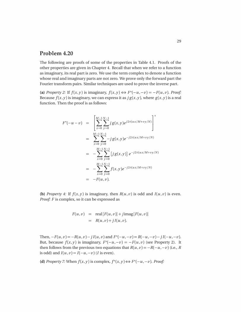
Problem 4.20
The following are proofs of some of the properties in Table 4.1. Proofs of theother properties are given in Chapter 4. Recall that when we refer to a functionas imaginary, its real part is zero. We use the term complex to denote a functionwhose real and imaginary parts are not zero. We prove only the forward part theFourier transform pairs. Similar techniques are used to prove the inverse part.
(a) Property 2: If f (x ,y ) is imaginary, f (x ,y )⇔ F ∗(−u ,−v ) = −F (u ,v ). Proof:Because f (x ,y ) is imaginary, we can express it as j g (x ,y ), where g (x ,y ) is a realfunction. Then the proof is as follows:
F ∗(−u − v ) =
⎡⎢⎣M−1∑
x=0
N−1∑y=0
j g (x ,y )e j 2π(u x/M+v y /N )
⎤⎥⎦∗
=M−1∑x=0
N−1∑y=0
−j g (x ,y )e−j 2π(u x/M+v y /N )
= −M−1∑x=0
N−1∑y=0
�j g (x ,y )
e−j 2π(u x/M+v y /N )
= −M−1∑x=0
N−1∑y=0
f (x ,y )e−j 2π(u x/M+v y /N )
= −F (u ,v ).
(b) Property 4: If f (x ,y ) is imaginary, then R(u ,v ) is odd and I (u ,v ) is even.Proof: F is complex, so it can be expressed as
F (u ,v ) = real [F (u ,v )] + j imag [F (u ,v )]
= R(u ,v )+ j I (u ,v ).
Then,−F (u ,v ) =−R(u ,v )− j I (u ,v ) and F ∗(−u ,−v ) = R(−u ,−v )− j I (−u ,−v ).But, because f (x ,y ) is imaginary, F ∗(−u ,−v ) = −F (u ,v ) (see Property 2). Itthen follows from the previous two equations that R(u ,v ) =−R(−u ,−v ) (i.e., Ris odd) and I (u ,v ) = I (−u ,−v ) (I is even).
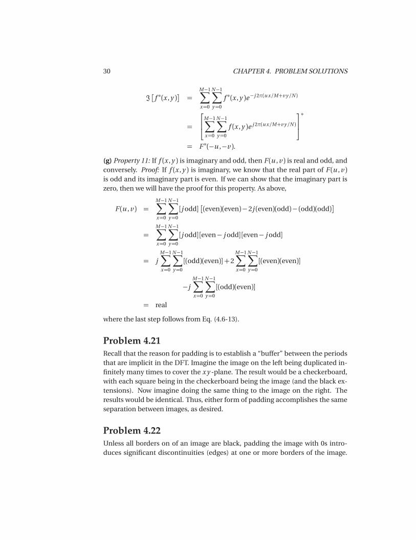
(d) Property 7: When f (x ,y ) is complex, f ∗(x ,y )⇔ F ∗(−u ,−v ). Proof:
30 CHAPTER 4. PROBLEM SOLUTIONS
ℑ� f ∗(x ,y )=
M−1∑x=0
N−1∑y=0
f ∗(x ,y )e−j 2π(u x/M+v y /N )
=
⎡⎢⎣M−1∑
x=0
N−1∑y=0
f (x ,y )e j 2π(u x/M+v y /N )
⎤⎥⎦∗
= F ∗(−u ,−v ).
(g) Property 11: If f (x ,y ) is imaginary and odd, then F (u ,v ) is real and odd, andconversely. Proof: If f (x ,y ) is imaginary, we know that the real part of F (u ,v )is odd and its imaginary part is even. If we can show that the imaginary part iszero, then we will have the proof for this property. As above,
F (u ,v ) =M−1∑x=0
N−1∑y=0
[j odd]�(even)(even)− 2j (even)(odd)− (odd)(odd)
=M−1∑x=0
N−1∑y=0
[j odd][even− j odd][even− j odd]
= jM−1∑x=0
N−1∑y=0
[(odd)(even)]+ 2M−1∑x=0
N−1∑y=0
[(even)(even)]
−jM−1∑x=0
N−1∑y=0
[(odd)(even)]
= real
where the last step follows from Eq. (4.6-13).
Problem 4.21Recall that the reason for padding is to establish a “buffer” between the periodsthat are implicit in the DFT. Imagine the image on the left being duplicated in-finitely many times to cover the x y -plane. The result would be a checkerboard,with each square being in the checkerboard being the image (and the black ex-tensions). Now imagine doing the same thing to the image on the right. Theresults would be identical. Thus, either form of padding accomplishes the sameseparation between images, as desired.
Problem 4.22Unless all borders on of an image are black, padding the image with 0s intro-duces significant discontinuities (edges) at one or more borders of the image.

31
These can be strong horizontal and vertical edges. These sharp transitions inthe spatial domain introduce high-frequency components along the vertical andhorizontal axes of the spectrum.
Problem 4.23(a) The averages of the two images are computed as follows:
f (x ,y ) =1
M N
M−1∑x=0
N−1∑y=0
f (x ,y )
and
f p (x ,y ) =1
PQ
P−1∑x=0
Q−1∑y=0
f p (x ,y )
=1
PQ
M−1∑x=0
N−1∑y=0
f (x ,y )
=M N
PQf (x ,y )
where the second step is result of the fact that the image is padded with 0s. Thus,the ratio of the average values is
r =PQ
M N
Thus, we see that the ratio increases as a function of PQ, indicating that theaverage value of the padded image decreases as a function of PQ. This is asexpected; padding an image with zeros decreases its average value.
Problem 4.25(a) From Eq. (4.4-10) and the definition of the 1-D DFT,
ℑ� f (x ) h(x )=
M−1∑x=0
f (x ) h(x )e−j 2πu x/M
=M−1∑x=0
M−1∑m=0
f (m )h(x −m )e−j 2πu x/M
=M−1∑m=0
f (m )M−1∑x=0
h(x −m )e−j 2πu x/M
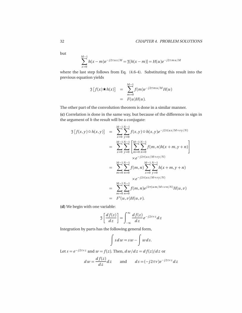
32 CHAPTER 4. PROBLEM SOLUTIONS
butM−1∑x=0
h(x −m )e−j 2πu x/M = ℑ[h(x −m )] =H (u )e−j 2πm u /M
where the last step follows from Eq. (4.6-4). Substituting this result into theprevious equation yields
ℑ� f (x ) h(x )=
M−1∑m=0
f (m )e−j 2πm u /M H (u )
= F (u )H (u ).
The other part of the convolution theorem is done in a similar manner.
(c) Correlation is done in the same way, but because of the difference in sign inthe argument of h the result will be a conjugate:
ℑ� f (x ,y ) h(x ,y )=
M−1∑x=0
N−1∑y=0
f (x ,y ) h(x ,y )e−j 2π(u x/M+v y /N )
=M−1∑x=0
N−1∑y=0
⎡⎣M−1∑
m=0
N−1∑n=0
f (m ,n )h(x +m ,y +n )
⎤⎦
×e−j 2π(u x/M+v y /N )
=M−1∑m=0
N−1∑n=0
f (m ,n )M−1∑x=0
N−1∑y=0
h(x +m ,y +n )
×e−j 2π(u x/M+v y /N )
=M−1∑m=0
N−1∑n=0
f (m ,n )e j 2π(u m/M+v n/N )H (u ,v )
= F ∗(u ,v )H (u ,v ).
(d) We begin with one variable:
ℑ�
d f (z )d z
�=
∫ ∞−∞
d f (z )d z
e−j 2πνz d z
Integration by parts has the following general form,∫s d w = s w −
∫w d s .
Let s = e−j 2πνz and w = f (z ). Then, d w /d z = d f (z )/d z or
d w =d f (z )
d zd z and d s = (−j 2πν )e−j 2πνz d z
33
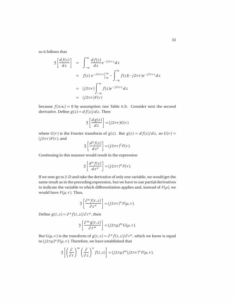
so it follows that
ℑ�
d f (z )d z
�=
∫ ∞−∞
d f (z )d z
e−j 2πνz d z
= f (z ) e−j 2πνz ∞∞−
∫ ∞−∞
f (z )(−j 2πν )e−j 2πνz d z
= (j 2πν )
∫ ∞−∞
f (z )e−j 2πνz d z
= (j 2πν )F (ν )
because f (±∞) = 0 by assumption (see Table 4.3). Consider next the secondderivative. Define g (z ) = d f (z )/d z . Then
ℑ�
d g (z )d z
�= (j 2πν )G (ν )
where G (ν ) is the Fourier transform of g (z ). But g (z ) = d f (z )/d z , so G (ν ) =(j 2πν )F (ν ), and
ℑ�
d 2 f (z )d z 2
�= (j 2πν )2F (ν ).
Continuing in this manner would result in the expression
ℑ�
d n f (z )d z n
�= (j 2πν )n F (ν ).
If we now go to 2-D and take the derivative of only one variable, we would get thesame result as in the preceding expression, but we have to use partial derivativesto indicate the variable to which differentiation applies and, instead of F (μ), wewould have F (μ,ν ). Thus,
ℑ�∂ n f (t ,z )∂ z n
�= (j 2πν )n F (μ,ν ).
Define g (t ,z ) = ∂ n f (t ,z )/∂ t n , then
ℑ�∂ m g (t ,z )∂ t m
�= (j 2πμ)m G (μ,ν ).
But G(μ,ν ) is the transform of g (t ,z ) = ∂ n f (t ,z )/∂ t n , which we know is equalto (j 2πμ)n F (μ,ν ). Therefore, we have established that
ℑ��∂
∂ t
�m �∂
∂ z
�n
f (t ,z )�= (j 2πμ)m (j 2πν )n F (μ,ν ).
34 CHAPTER 4. PROBLEM SOLUTIONS
Because the Fourier transform is unique, we know that the inverse transformof the right of this equation would give the left, so the equation constitutes aFourier transform pair (keep in mind that we are dealing with continuous vari-ables).
Problem 4.26
(b) As the preceding derivation shows, the Laplacian filter applies to continuousvariables. We can generate a filter for using with the DFT simply by samplingthis function:
H (u ,v ) =−4π2(u 2+ v 2)
for u = 0,1,2, . . . ,M − 1 and v = 0,1,2, . . . ,N − 1. When working with centeredtransforms, the Laplacian filter function in the frequency domain is expressedas
H (u ,v ) =−4π2([u −M/2]2+[v −N /2]2).
In summary, we have the following Fourier transform pair relating the Laplacianin the spatial and frequency domains:
∇2 f (x ,y )⇔−4π2([u −M/2]2+[v −N /2]2)F (u ,v )
where it is understood that the filter is a sampled version of a continuous func-tion.
(c) The Laplacian filter is isotropic, so its symmetry is approximated much closerby a Laplacian mask having the additional diagonal terms, which requires a −8in the center so that its response is 0 in areas of constant intensity.
Problem 4.27(a) The spatial average (excluding the center term) is
g (x ,y ) =1
4
�f (x ,y + 1)+ f (x + 1,y )+ f (x − 1,y )+ f (x ,y − 1)
.
From property 3 in Table 4.3,
G (u ,v ) =1
4
�e j 2πv /N + e j 2πu /M + e−j 2πu /M + e−j 2πv /N
F (u ,v )
= H (u ,v )F (u ,v )
where
H (u ,v ) =1
2[cos(2πu /M )+ cos(2πv /N )]

35
is the filter transfer function in the frequency domain.
(b) To see that this is a lowpass filter, it helps to express the preceding equationin the form of our familiar centered functions:
H (u ,v ) =1
2[cos(2π[u −M/2])/M )+ cos(2π[v −N /2]/N )] .
Consider one variable for convenience. As u ranges from 0 to M − 1, the valueof cos(2π[u −M/2]/M ) starts at −1, peaks at 1 when u = M/2 (the center ofthe filter) and then decreases to −1 again when u =M . Thus, we see that theamplitude of the filter decreases as a function of distance from the origin of thecentered filter, which is the characteristic of a lowpass filter. A similar argumentis easily carried out when considering both variables simultaneously.
Problem 4.30The answer is no. The Fourier transform is a linear process, while the squareand square roots involved in computing the gradient are nonlinear operations.The Fourier transform could be used to compute the derivatives as differences(as in Problem 4.28), but the squares, square root, or absolute values must becomputed directly in the spatial domain.
Problem 4.31We want to show that
ℑ−1�
Ae−(μ2+ν2)/2σ2 = A2πσ2e−2π2σ2(t 2+z 2).
The explanation will be clearer if we start with one variable. We want to showthat, if
H (μ) = e−μ2/2σ2
then
h(t ) = ℑ−1 �H (μ)
=
∫ ∞−∞
e−μ2/2σ2e j 2tμt dμ
=�
2πσ−2π2σ2t 2.
We can express the integral in the preceding equations as
h(t ) =
∫ ∞−∞
e−1
2σ2 [μ2−j 4πσ2μt ]dμ.

36 CHAPTER 4. PROBLEM SOLUTIONS
Making use of the identity
e− (2π)2σ2t 2
2 e(2π)2σ2t 2
2 = 1
in the preceding integral yields
h(t ) = e− (2π)2σ2t 2
2
∫ ∞−∞
e−1
2σ2 [μ2−j 4πσ2μt−(2π)2σ4t 2]dμ.
= e− (2π)2σ2t 2
2
∫ ∞−∞
e−1
2σ2 [μ−j 2πσ2t ]2dμ.
Next, we make the change of variables r = μ− j 2πσ2t . Then, d r = dμ and thepreceding integral becomes
h(t ) = e− (2π)2σ2t 2
2
∫ ∞−∞
e−r 2
2σ2 d r.
Finally, we multiply and divide the right side of this equation by�
2πσand ob-tain
h(t ) =�
2πσe− (2π)2σ2t 2
2
⎡⎣ 1�
2πσ
∫ ∞−∞
e−r 2
2σ2 d r
⎤⎦ .
The expression inside the brackets is recognized as the Gaussian probabilitydensity function whose value from -∞ to∞ is 1. Therefore,
h(t ) =�
2πσe−2π2σ2t 2.
With the preceding results as background, we are now ready to show that
h(t ,z ) = ℑ−1�
Ae−(μ2+ν2)/2σ2 = A2πσ2e−2π2σ2(t 2+z 2).
By substituting directly into the definition of the inverse Fourier transform wehave:
h(t ,z ) =
∫ ∞−∞
∫ ∞−∞
Ae−(μ2+ν2)/2σ2e j 2π(μt+νz )dμdν
=
∫ ∞−∞
⎡⎣∫ ∞−∞
Ae
�− μ2
2σ2 +j 2πμt�
dμ
⎤⎦e
�− ν2
2σ2 +j 2πνz�
dν .

37
The integral inside the brackets is recognized from the previous discussion to beequal to A
�2πσe−2π2σ2t 2 . Then, the preceding integral becomes
h(t ,z ) =A�
2πσe−2π2σ2t 2
∫ ∞−∞
e�− ν2
2σ2 +j 2πνz�
dν .
We now recognize the remaining integral to be equal to�
2πσe−2π2σ2z 2 , fromwhich we have the final result:
h(t ,z ) =�
A�
2πσe−2π2σ2t 2���2πσe−2π2σ2z 2�
= A2πσ2e−2π2σ2(t 2+z 2).
Problem 4.35With reference to Eq. (4.9-1), all the highpass filters in discussed in Section 4.9can be expressed a 1 minus the transfer function of lowpass filter (which weknow do not have an impulse at the origin). The inverse Fourier transform of 1gives an impulse at the origin in the highpass spatial filters.
Problem 4.37(a) One application of the filter gives:
G (u ,v ) = H (u ,v )F (u ,v )
= e−D2(u ,v )/2D20 F (u ,v ).
Similarly, K applications of the filter would give
GK (u ,v ) = e−K D2(u ,v )/2D20 F (u ,v ).
The inverse DFT of GK (u ,v ) would give the image resulting from K passes ofthe Gaussian filter. If K is “large enough,” the Gaussian LPF will become a notchpass filter, passing only F (0,0). We know that this term is equal to the averagevalue of the image. So, there is a value of K after which the result of repeatedlowpass filtering will simply produce a constant image. The value of all pixelson this image will be equal to the average value of the original image. Note thatthe answer applies even as K approaches infinity. In this case the filter will ap-proach an impulse at the origin, and this would still give us F (0,0) as the resultof filtering.

38 CHAPTER 4. PROBLEM SOLUTIONS
Problem 4.41Because M = 2n , we can write Eqs. (4.11-16) and (4.11-17) as
m (n ) =1
2M n
anda (n ) =M n .
Proof by induction begins by showing that both equations hold for n = 1:
m (1) =1
2(2)(1) = 1 and a (1) = (2)(1) = 2.
We know these results to be correct from the discussion in Section 4.11.3. Next,we assume that the equations hold for n . Then, we are required to prove thatthey also are true for n + 1. From Eq. (4.11-14),
m (n + 1) = 2m (n )+ 2n .
Substituting m (n ) from above,
m (n + 1) = 2
�1
2M n
�+ 2n
= 2
�1
22n n
�+ 2n
= 2n (n + 1)
=1
2
�2n+1
�(n + 1).
Therefore, Eq. (4.11-16) is valid for all n .From Eq. (4.11-17),
a (n + 1) = 2a (n )+ 2n+1.
Substituting the above expression for a (n ) yields
a (n + 1) = 2M n + 2n+1
= 2(2n n )+ 2n+1
= 2n+1(n + 1)
which completes the proof.

NOTICE This manual is intended for your personal use only. Copying, printing, posting, or any form of printed or electronic distribution of any part of this manual constitutes a violation of copyright law. As a security measure, this manual was encrypted during download with the serial number of your book, and with your personal information. Any printed or electronic copies of this file will bear that encryption, which will tie the copy to you. Please help us defeat piracy of intellectual property, one of the principal reasons for the increase in the cost of books. -------------------------------

Chapter 5
Problem Solutions
Problem 5.1The solutions are shown in Fig. P5.1, from left to right.
Figure P5.1
Problem 5.3The solutions are shown in Fig. P5.3, from left to right.
Figure P5.3
39

40 CHAPTER 5. PROBLEM SOLUTIONS
Problem 5.5The solutions are shown in Fig. P5.5, from left to right.
Figure P5.5
Problem 5.7The solutions are shown in Fig. P5.7, from left to right.
Figure P5.7
Problem 5.9The solutions are shown in Fig. P5.9, from left to right.
Figure P5.9
41
Problem 5.10(a) The key to this problem is that the geometric mean is zero whenever anypixel is zero. Draw a profile of an ideal edge with a few points valued 0 and a fewpoints valued 1. The geometric mean will give only values of 0 and 1, whereasthe arithmetic mean will give intermediate values (blur).
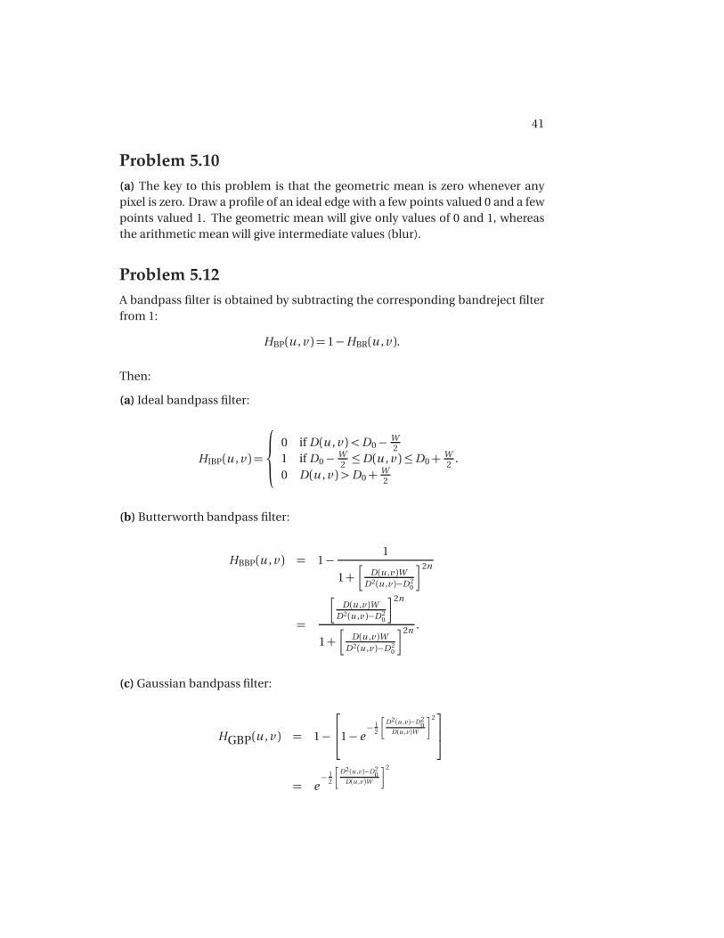
Problem 5.12A bandpass filter is obtained by subtracting the corresponding bandreject filterfrom 1:
HBP(u ,v ) = 1−HBR(u ,v ).
Then:
(a) Ideal bandpass filter:
HIBP(u ,v ) =
⎧⎨⎩
0 if D(u ,v )<D0− W2
1 if D0− W2≤D(u ,v )≤D0+ W
2.
0 D(u ,v )>D0+ W2
(b) Butterworth bandpass filter:
HBBP(u ,v ) = 1− 1
1+
D(u ,v )WD2(u ,v )−D2
0
!2n
=
D(u ,v )W
D2(u ,v )−D20
!2n
1+
D(u ,v )WD2(u ,v )−D2
0
!2n .
(c) Gaussian bandpass filter:
HGBP(u ,v ) = 1−⎡⎢⎣1− e
− 12
�D2 (u ,v )−D2
0D(u ,v )W
�2⎤⎥⎦
= e− 1
2
�D2 (u ,v )−D2
0D(u ,v )W
�2
42 CHAPTER 5. PROBLEM SOLUTIONS
Problem 5.14We proceed as follows:
F (u ,v ) =
∫∫ ∞−∞
f (x ,y )e−j 2π(u x +v y )d x d y
=
∫∫ ∞−∞
A sin(u 0x + v0y )e−j 2π(u x +v y )d x d y .
Using the exponential definition of the sine function,
sinθ =1
2j
�e j θ − e−j θ
�
gives us
F (u ,v ) =−j A
2
∫∫ ∞−∞
�e j (u 0x +v0y )− e−j (u 0x +v0y )
e−j 2π(u x +v y )d x d y
=−j A
2
⎡⎣∫∫ ∞
−∞e j 2π(u 0x/2π+v0y /2π)e−j 2π(u x +v y )d x d y
⎤⎦−
j A
2
⎡⎣∫∫ ∞
−∞e−j 2π(u 0x/2π+v0y /2π)e−j 2π(u x +v y )d x d y
⎤⎦ .
These are the Fourier transforms of the functions
1× e j 2π(u 0x/2π+v0y /2π)
and1× e−j 2π(u 0x/2π+v0y /2π)
respectively. The Fourier transform of the 1 gives an impulse at the origin, andthe exponentials shift the origin of the impulse, as discussed in Section 4.6.3 andTable 4.3. Thus,
F (u ,v ) =−j A
2
δ�
u − u 0
2π,v − v0
2π
�−δ
�u +
u 0
2π,v +
v0
2π
�!.
Problem 5.16From Eq. (5.5-13),
g (x ,y ) =
∫∫ ∞−∞
f (α,β )h(x −α,y −β )dαdβ .

43
It is given that f (x ,y ) = δ(x −a ), so f (α,β ) = δ(α−a ). Then, using the impulseresponse given in the problem statement,
g (x ,y ) =
∫ ∫ ∞−∞δ(α−a )e−
"(x−α)2+(y−β)2
#dαdβ
=
∫∫ ∞−∞δ(α−a )e−[(x−α)2] e−
"(y−β)2
#dαdβ
=
∫ ∞−∞δ(α−a )e−[(x−α)2]dα
∫ ∞−∞
e−"(y−β)2
#dβ
= e−[(x−a )2]∫ ∞−∞
e−"(y−β)2#dβ
where we used the fact that the integral of the impulse is nonzero only whenα= a . Next, we note that
∫ ∞−∞
e−"(y−β)2#dβ =
∫ ∞−∞
e−"(β−y )2
#dβ
which is in the form of a constant times a Gaussian density with variance σ2 =1/2 or standard deviationσ= 1/
�2. In other words,
e−"(β−y )2
#=$
2π(1/2)
⎡⎣ 1$
2π(1/2)e−(1/2)
�(β−y )2(1/2)
�⎤⎦ .
The integral from minus to plus infinity of the quantity inside the brackets is 1,so
g (x ,y ) =�πe−[(x−a )2]
which is a blurred version of the original image.
44 CHAPTER 5. PROBLEM SOLUTIONS
Problem 5.18Following the procedure in Section 5.6.3,
H (u ,v ) =
∫ T
0
e−j 2πu x0(t )d t
=
∫ T
0
e−j 2πu [(1/2)a t 2]d t
=
∫ T
0
e−jπu a t 2d t
=
∫ T
0
�cos(πu a t 2)− j sin(πu a t 2)
d t
=
%T 2
2πu a T 2
�C (�πu a T )− j S(
�πu a T )
where
C (z ) =
&2π
T
∫ z
0
cos t 2d t
and
S(z ) =
&2
π
∫ z
0
sin t 2d t .
These are Fresnel cosine and sine integrals. They can be found, for example,the Handbook of Mathematical Functions, by Abramowitz, or other similar ref-erence.
Problem 5.20Measure the average value of the background. Set all pixels in the image, ex-cept the cross hairs, to that intensity value. Denote the Fourier transform ofthis image by G (u ,v ). Because the characteristics of the cross hairs are givenwith a high degree of accuracy, we can construct an image of the background(of the same size) using the background intensity levels determined previously.We then construct a model of the cross hairs in the correct location (determinedfrom the given image) using the dimensions provided and intensity level of thecross hairs. Denote by F (u ,v ) the Fourier transform of this new image . Theratio G (u ,v )/F (u ,v ) is an estimate of the blurring function H (u ,v ). In the likelyevent of vanishing values in F (u ,v ), we can construct a radially-limited filter us-ing the method discussed in connection with Fig. 5.27. Because we know F (u ,v )
45
and G (u ,v ), and an estimate of H (u ,v ), we can refine our estimate of the blur-ring function by substituting G and H in Eq. (5.8-3) and adjusting K to get asclose as possible to a good result for F (u ,v ) (the result can be evaluated visuallyby taking the inverse Fourier transform). The resulting filter in either case canthen be used to deblur the image of the heart, if desired.
Problem 5.22This is a simple plug in problem. Its purpose is to gain familiarity with the vari-ous terms of the Wiener filter. From Eq. (5.8-3),
HW(u ,v ) =
'1
H (u ,v )|H (u ,v )|2|H (u ,v )|2+K
(
where
|H (u ,v )|2 = H ∗(u ,v )H (u ,v )
= H 2(u ,v )
= 64π6σ4(u 2+ v 2)2e−4π2σ2(u 2+v 2).
Then,
HW(u ,v ) =−⎡⎣ −8π3σ2(u 2+ v 2)e−2π2σ2(u 2+v 2)�
64π6σ4(u 2+ v 2)2e−4π2σ2(u 2+v 2) +K
⎤⎦ .
Problem 5.25(a) It is given that ��F (u ,v )
��2 = |R(u ,v )|2 |G (u ,v )|2 .
From Problem 5.24 (recall that the image and noise are assumed to be uncorre-lated), ��F (u ,v )
��2 = |R(u ,v )|2 �|H (u ,v )|2 |F (u ,v )|2+ |N (u ,v )|2 .
Forcing��F (u ,v )
��2 to equal |F (u ,v )|2 gives
R(u ,v ) =
' |F (u ,v )|2|H (u ,v )|2 |F (u ,v )|2+ |N (u ,v )|2
(1/2
.
Problem 5.27The basic idea behind this problem is to use the camera and representative coinsto model the degradation process and then utilize the results in an inverse filteroperation. The principal steps are as follows:
46 CHAPTER 5. PROBLEM SOLUTIONS
1. Select coins as close as possible in size and content as the lost coins. Selecta background that approximates the texture and brightness of the photosof the lost coins.
2. Set up the museum photographic camera in a geometry as close as possi-ble to give images that resemble the images of the lost coins (this includespaying attention to illumination). Obtain a few test photos. To simplifyexperimentation, obtain a TV camera capable of giving images that re-semble the test photos. This can be done by connecting the camera toan image processing system and generating digital images, which will beused in the experiment.
3. Obtain sets of images of each coin with different lens settings. The re-sulting images should approximate the aspect angle, size (in relation tothe area occupied by the background), and blur of the photos of the lostcoins.
4. The lens setting for each image in (3) is a model of the blurring processfor the corresponding image of a lost coin. For each such setting, removethe coin and background and replace them with a small, bright dot on auniform background, or other mechanism to approximate an impulse oflight. Digitize the impulse. Its Fourier transform is the transfer function ofthe blurring process.
5. Digitize each (blurred) photo of a lost coin, and obtain its Fourier trans-form. At this point, we have H (u ,v ) and G (u ,v ) for each coin.
6. Obtain an approximation to F (u ,v ) by using a Wiener filter. Equation(5.8-3) is particularly attractive because it gives an additional degree offreedom (K ) for experimenting.
7. The inverse Fourier transform of each approximation F (u ,v ) gives the re-stored image for a coin. In general, several experimental passes of thesebasic steps with various different settings and parameters are required toobtain acceptable results in a problem such as this.
Problem 5.28(b) The solution is shown in the following figure.The solutions are shown in Fig.P5.28. In each figure the horizontal axis isρ and the vertical axis is θ , with θ = 0◦at the bottom and going up to 180◦. The fat lobes occur at 45◦ and the singlepoint of intersection is at 135◦. The intensity at that point is double the intensityof all other points.

47
Figure P5.28
Problem 5.30(a) From Eq. (5.11-3),
ℜ f (x ,y )�= g (ρ,θ ) =
∫ ∞−∞
∫ ∞−∞
f (x ,y )δ(x cosθ + y sinθ −ρ)d x d y
=
∫ ∞−∞
∫ ∞−∞δ(x ,y )δ(x cosθ + y sinθ −ρ)d x d y
=
∫ ∞−∞
∫ ∞−∞
1×δ(0−ρ)d x d y
=
)1 ifρ = 00 otherwise.
where the third step follows from the fact thatδ(x ,y ) is zero if x and/or y are notzero.
Problem 5.31
(a) From Section 2.6, we know that an operator, O, is linear if O(a f 1 + b f 2) =aO(f 1)+bO(f 2). From the definition of the Radon transform in Eq. (5.11-3),
O(a f 1+b f 2) =
∫ ∞−∞
∫ ∞−∞(a f 1+b f 2)δ(x cosθ + y sinθ −ρ)d x d y
= a
∫ ∞−∞
∫ ∞−∞
f 1δ(x cosθ + y sinθ −ρ)d x d y
+b
∫ ∞−∞
∫ ∞−∞
f 2δ(x cosθ + y sinθ −ρ)d x d y
= aO(f 1)+bO(f 2)
thus showing that the Radon transform is a linear operation.

48 CHAPTER 5. PROBLEM SOLUTIONS
(c) From Chapter 4 (Problem 4.11), we know that the convolution of two func-tion f and h is defined as
c (x ,y ) = f (x ,y ) h(x ,y )
=
∫ ∞−∞
∫ ∞−∞
f (α,β )h(x −α,y −β )dαdβ .
We want to show that ℜ{c} = ℜ f� ℜ{h} ,where ℜ denotes the Radon trans-
form. We do this by substituting the convolution expression into Eq. (5.11-3).That is,
ℜ{c} =∫ ∞−∞
∫ ∞−∞
⎡⎣∫ ∞−∞
∫ ∞−∞
f (α,β )h(x −α,y −β )dαdβ
⎤⎦
×δ(x cosθ + y sinθ −ρ)d x d y
=
∫α
∫β
f (α,β )
×⎡⎣∫
x
∫y
h(x −α,y −β )δ(x cosθ + y sinθ −ρ)d x d y
⎤⎦dαdβ
where we used the subscripts in the integrals for clarity between the integralsand their variables. All integrals are understood to be between−∞ and∞. Work-ing with the integrals inside the brackets with x ′ = x −α and y ′ = y −β we have∫
x
∫y
h(x −α,y −β )δ(x cosθ + y sinθ −ρ)d x d y
=∫
x ′∫
y ′ h(x′,y ′)δ(x ′ cosθ + y ′ sinθ − [ρ−αcosθ −β sinθ ])d x ′d y ′
=ℜ{h} (ρ−αcosθ −β sinθ ,θ ).
We recognize the second integral as the Radon transform of h, but instead ofbeing with respect to ρ and θ , it is a function of ρ − αcosθ − β sinθ and θ .The notation in the last line is used to indicate “the Radon transform of h as afunction of ρ−αcosθ −β sinθ and θ .” Then,
ℜ{c} =∫α
∫β
f (α,β )
×⎡⎣∫
x
∫y
h(x −α,y −β )δ(x cosθ + y sinθ −ρ)d x d y
⎤⎦dαdβ
=
∫α
∫β
f (α,β )ℜ{h} (ρ−ρ′,θ )dαdβ

49
where ρ′ = αcosθ +β sinθ . Then, based on the properties of the impulse, wecan write
ℜ{h} (ρ−ρ′,θ ) =∫ρ′ℜ{h} (ρ−ρ′,θ )δ(αcosθ +β sinθ −ρ′)dρ′.
Then,
ℜ{c}=∫α
∫β
f (α,β )�ℜ{h} (ρ−ρ′,θ )dαdβ
=
∫α
∫β
f (α,β )
×⎡⎣∫
ρ′ℜ{h} (ρ−ρ′,θ )δ(αcosθ +β sinθ −ρ′)dρ′
⎤⎦dαdβ
=
∫ρ′ℜ{h} (ρ−ρ′,θ )
⎡⎣∫
α
∫β
f (α,β )δ(αcosθ +β sinθ −ρ′)dαdβ
⎤⎦dρ′
=
∫ρ′ℜ{h} (ρ−ρ′,θ )ℜ f
�(ρ′,θ )dρ′
= ℜ f� ℜ{h}
where the fourth step follows from the definition of the Radon transform and thefifth step follows from the definition of convolution. This completes the proof.
Problem 5.33The argument of function s in Eq.(5.11-24) may be written as:
r cos(β +α−ϕ)−D sinα= r cos(β −ϕ)cosα− [r sin(β −ϕ)+D]sinα.
From Fig. 5.47,
R cosα′ = R + r sin(β −ϕ)R sinα′ = r cos(β −ϕ).
Then, substituting in the earlier expression,
r cos(β +α−ϕ)−R sinα = R sinα′ cosα−R cosα′ sinα
= R(sinα′ cosα− cosα′ sinα)
= R sin(α′ −α)which agrees with Eq. (5.11-25).

NOTICE This manual is intended for your personal use only. Copying, printing, posting, or any form of printed or electronic distribution of any part of this manual constitutes a violation of copyright law. As a security measure, this manual was encrypted during download with the serial number of your book, and with your personal information. Any printed or electronic copies of this file will bear that encryption, which will tie the copy to you. Please help us defeat piracy of intellectual property, one of the principal reasons for the increase in the cost of books. -------------------------------

Chapter 6
Problem Solutions
Problem 6.2Denote by c the given color, and let its coordinates be denoted by (x0,y0). Thedistance between c and c1 is
d (c ,c1) =�(x0−x1)2+
�y0− y1
�2 1/2
.
Similarly the distance between c1 and c2
d (c1,c2) =�(x1−x2)2+
�y1− y2
�2 1/2
.
The percentage p1 of c1 in c is
p1 =d (c1,c2)−d (c ,c1)
d (c1,c2)× 100.
The percentage p2 of c2 is simply p2 = 100−p1. In the preceding equation wesee, for example, that when c = c1, then d (c ,c1) = 0 and it follows that p1 = 100%and p2 = 0%. Similarly, when d (c ,c1) = d (c1,c2), it follows that p1 = 0% and p2 =100%. Values in between are easily seen to follow from these simple relations.
Problem 6.4Use color filters that are sharply tuned to the wavelengths of the colors of thethree objects. With a specific filter in place, only the objects whose color cor-responds to that wavelength will produce a significant response on the mono-chrome camera. A motorized filter wheel can be used to control filter positionfrom a computer. If one of the colors is white, then the response of the threefilters will be approximately equal and high. If one of the colors is black, theresponse of the three filters will be approximately equal and low.
51
52 CHAPTER 6. PROBLEM SOLUTIONS
Figure P6.6
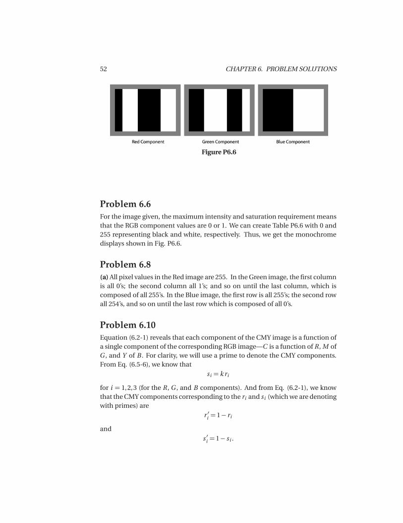
Problem 6.6For the image given, the maximum intensity and saturation requirement meansthat the RGB component values are 0 or 1. We can create Table P6.6 with 0 and255 representing black and white, respectively. Thus, we get the monochromedisplays shown in Fig. P6.6.
Problem 6.8(a) All pixel values in the Red image are 255. In the Green image, the first columnis all 0’s; the second column all 1’s; and so on until the last column, which iscomposed of all 255’s. In the Blue image, the first row is all 255’s; the second rowall 254’s, and so on until the last row which is composed of all 0’s.
Problem 6.10Equation (6.2-1) reveals that each component of the CMY image is a function ofa single component of the corresponding RGB image—C is a function of R , M ofG , and Y of B . For clarity, we will use a prime to denote the CMY components.From Eq. (6.5-6), we know that
si = k ri
for i = 1,2,3 (for the R , G , and B components). And from Eq. (6.2-1), we knowthat the CMY components corresponding to the ri and si (which we are denotingwith primes) are
r ′i = 1− ri
and
s ′i = 1− si .

53
Thus,
ri = 1− r ′iand
s ′i = 1− si = 1−k ri = 1−k�
1− r ′i�
so that
s ′i = k r ′i +(1−k ) .
Problem 6.12Using Eqs. (6.2-2) through (6.2-4), we get the results shown in Table P6.12. Notethat, in accordance with Eq. (6.2-2), hue is undefined when R =G = B since θ =cos−1 (0/0). In addition, saturation is undefined when R =G = B = 0 since Eq.(6.2-3) yields S = 1− 3min (0)/(3× 0) = 1− (0/0). Thus, we get the monochromedisplay shown in Fig. P6.12.
Table P6.12Color R G B H S I Mono H Mono S Mono IBlack 0 0 0 – 0 0 – – 0Red 1 0 0 0 1 0.33 0 255 85
Yellow 1 1 0 0.17 1 0.67 43 255 170Green 0 1 0 0.33 1 0.33 85 255 85Cyan 0 1 1 0.5 1 0.67 128 255 170Blue 0 0 1 0.67 1 0.33 170 255 85
Magenta 1 0 1 0.83 1 0.67 213 255 170White 1 1 1 – 0 1 – 0 255
Gray 0.5 0.5 0.5 – 0 0.5 – 0 128
Figure P6.12
54 CHAPTER 6. PROBLEM SOLUTIONS
Problem 6.14There are two important aspects to this problem. One is to approach it in theHSI space and the other is to use polar coordinates to create a hue image whosevalues grow as a function of angle. The center of the image is the middle of what-ever image area is used. Then, for example, the values of the hue image alonga radius when the angle is 0◦ would be all 0’s. Then the angle is incrementedby, say, one degree, and all the values along that radius would be 1’s, and so on.Values of the saturation image decrease linearly in all radial directions from theorigin. The intensity image is just a specified constant. With these basics inmind it is not difficult to write a program that generates the desired result.
Problem 6.16(a) It is given that the colors in Fig. 6.16(a) are primary spectrum colors. It also isgiven that the gray-level images in the problem statement are 8-bit images. Thelatter condition means that hue (angle) can only be divided into a maximumnumber of 256 values. Because hue values are represented in the interval from0◦ to 360◦ this means that for an 8-bit image the increments between contiguoushue values are now 360/255. Another way of looking at this is that the entire [0,360] hue scale is compressed to the range [0, 255]. Thus, for example, yellow(the first primary color we encounter), which is 60◦ now becomes 43 (the closestinteger) in the integer scale of the 8-bit image shown in the problem statement.Similarly, green, which is 120◦ becomes 85 in this image. From this we easilycompute the values of the other two regions as being 170 and 213. The region inthe middle is pure white [equal proportions of red green and blue in Fig. 6.61(a)]so its hue by definition is 0. This also is true of the black background.
Problem 6.18Using Eq. (6.2-3), we see that the basic problem is that many different colorshave the same saturation value. This was demonstrated in Problem 6.12, wherepure red, yellow, green, cyan, blue, and magenta all had a saturation of 1. Thatis, as long as any one of the RGB components is 0, Eq. (6.2-3) yields a saturationof 1.
Consider RGB colors (1,0,0) and (0,0.59,0), which represent shades of redand green. The HSI triplets for these colors [per Eq. (6.4-2) through (6.4-4)] are(0,1,0.33) and (0.33,1,0.2), respectively. Now, the complements of the begin-ning RGB values (see Section 6.5.2) are (0,1,1) and (1,0.41,1), respectively; thecorresponding colors are cyan and magenta. Their HSI values [per Eqs. (6.4-2)through (6.4-4)] are (0.5,1,0.66) and (0.83,0.48,0.8), respectively. Thus, for the
55
red, a starting saturation of 1 yielded the cyan “complemented” saturation of1, while for the green, a starting saturation of 1 yielded the magenta “comple-mented” saturation of 0.48. That is, the same starting saturation resulted in twodifferent “complemented” saturations. Saturation alone is not enough informa-tion to compute the saturation of the complemented color.
Problem 6.20The RGB transformations for a complement [from Fig. 6.33(b)] are:
si = 1− ri
where i = 1,2,3 (for the R , G , and B components). But from the definition of theCMY space in Eq. (6.2-1), we know that the CMY components corresponding tori and si , which we will denote using primes, are
r ′i = 1− ri
s ′i = 1− si .
Thus,
ri = 1− r ′iand
s ′i = 1− si = 1− (1− ri ) = 1− �1− �1− r ′i��
so that
s ′ = 1− r ′i .
Problem 6.22Based on the discussion is Section 6.5.4 and with reference to the color wheelin Fig. 6.32, we can decrease the proportion of yellow by (1) decreasing yellow,(2) increasing blue, (3) increasing cyan and magenta, or (4) decreasing red andgreen.
Problem 6.24The simplest approach conceptually is to transform every input image to the HSIcolor space, perform histogram specification per the discussion in Section 3.3.2on the intensity (I ) component only (leaving H and S alone), and convert theresulting intensity component with the original hue and saturation componentsback to the starting color space.

56 CHAPTER 6. PROBLEM SOLUTIONS
Problem 6.27(a) The cube is composed of six intersecting planes in RGB space. The generalequation for such planes is
a z R +b zG + c z B +d = 0
where a , b , c , and d are parameters and the z ’s are the components of any point(vector) z in RGB space lying on the plane. If an RGB point z does not lie on theplane, and its coordinates are substituted in the preceding equation, the equa-tion will give either a positive or a negative value; it will not yield zero. We saythat z lies on the positive or negative side of the plane, depending on whetherthe result is positive or negative. We can change the positive side of a plane bymultiplying its coefficients (except d ) by −1. Suppose that we test the point agiven in the problem statement to see whether it is on the positive or negativeside each of the six planes composing the box, and change the coefficients ofany plane for which the result is negative. Then, a will lie on the positive side ofall planes composing the bounding box. In fact all points inside the boundingbox will yield positive values when their coordinates are substituted in the equa-tions of the planes. Points outside the box will give at least one negative (or zeroif it is on a plane) value. Thus, the method consists of substituting an unknowncolor point in the equations of all six planes. If all the results are positive, thepoint is inside the box; otherwise it is outside the box. A flow diagram is askedfor in the problem statement to make it simpler to evaluate the student’s line ofreasoning.

NOTICE This manual is intended for your personal use only. Copying, printing, posting, or any form of printed or electronic distribution of any part of this manual constitutes a violation of copyright law. As a security measure, this manual was encrypted during download with the serial number of your book, and with your personal information. Any printed or electronic copies of this file will bear that encryption, which will tie the copy to you. Please help us defeat piracy of intellectual property, one of the principal reasons for the increase in the cost of books. -------------------------------

Chapter 7
Problem Solutions
Problem 7.2
A mean approximation pyramid is created by forming 2×2 block averages. Sincethe starting image is of size 4× 4, J = 2 and f
�x ,y
�is placed in level 2 of the
mean approximation pyramid. The level 1 approximation is (by taking 2×2 blockaverages over f
�x ,y
�and subsampling)
'3.5 5.5
11.5 13.5
(
and the level 0 approximation is similarly [8.5]. The completed mean approxi-mation pyramid is
⎡⎢⎢⎢⎣
1 2 3 45 6 7 89 10 11 12
13 14 15 16
⎤⎥⎥⎥⎦'
3.5 5.511.5 13.5
([8.5] .
Pixel replication is used in the generation of the complementary prediction resid-ual pyramid. Level 0 of the prediction residual pyramid is the lowest resolu-tion approximation, [8.5]. The level 2 prediction residual is obtained by upsam-pling the level 1 approximation and subtracting it from the level 2 approxima-
57

58 CHAPTER 7. PROBLEM SOLUTIONS
tion (original image). Thus, we get⎡⎢⎢⎢⎣
1 2 3 45 6 7 89 10 11 12
13 14 15 16
⎤⎥⎥⎥⎦−
⎡⎢⎢⎢⎣
3.5 3.5 5.5 5.53.5 3.5 5.5 5.5
11.5 11.5 13.5 13.511.5 11.5 13.5 13.5
⎤⎥⎥⎥⎦ =
⎡⎢⎢⎢⎣−2.5 −1.5 −2.5 −1.51.5 2.5 1.5 2.5−2.5 −1.5 −2.5 −1.51.5 2.5 1.5 2.5
⎤⎥⎥⎥⎦ .
Similarly, the level 1 prediction residual is obtained by upsampling the level 0approximation and subtracting it from the level 1 approximation to yield'
3.5 5.511.5 13.5
(−'
8.5 8.58.5 8.5
(=
' −5 −33 5
(.
The prediction residual pyramid is therefore⎡⎢⎢⎢⎣−2.5 −1.5 −2.5 −1.51.5 2.5 1.5 2.5−2.5 −1.5 −2.5 −1.51.5 2.5 1.5 2.5
⎤⎥⎥⎥⎦' −5 −3
3 5
([8.5] .
Problem 7.3The number of elements in a J + 1 level pyramid where N = 2J is bounded by43 N 2 or 4
3
�2J�2 = 4
3 22J (see Section 7.1.1):
22J
+1+
1
(4)1+
1
(4)2+ ...+
1
(4) J
,≤ 4
322J
for J > 0. We can generate the following table:
J Pyramid Elements Compression Ratio0 1 11 5 5/4 = 1.252 21 21/16 = 1.31253 85 85/64 = 1.328...
......
∞ 4/3 = 1.33
All but the trivial case, J = 0, are expansions. The expansion factor is a functionof J and bounded by 4/3 or 1.33.
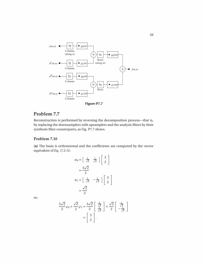
59
� g0(m)
� g1(m)
f(m,n)
a(m,n) 2 � g0(n)
� g1(n)
� g0(n)
� g1(n)
dV(m,n)
dH(m,n)
dD(m,n)
Rows(along m)
Rows
Columns(along n)
Columns
Columns
Columns
2
2
2
2
2
Figure P7.7
Problem 7.7Reconstruction is performed by reversing the decomposition process—that is,by replacing the downsamplers with upsamplers and the analysis filters by theirsynthesis filter counterparts, as Fig. P7.7 shows.
Problem 7.10
(a) The basis is orthonormal and the coefficients are computed by the vectorequivalent of Eq. (7.2-5):
α0 =�
1�2
1�2
' 32
(
=5�
2
2
α1 =�
1�2− 1�
2
' 32
(
=
�2
2so,
5�
2
2ϕ0+
�2
2ϕ1 =
5�
2
2
' 1�2
1�2
(+
�2
2
' 1�2− 1�
2
(
=
'32
(.

60 CHAPTER 7. PROBLEM SOLUTIONS
Problem 7.13From Eq. (7.2-19), we find that
ψ3,3(x ) = 23/2ψ(23x − 3)
= 2�
2ψ(8x − 3)
and using the Haar wavelet function definition from Eq. (7.2-30), obtain the plotin Fig. P7.13.
To expressψ3,3 (x ) as a function of scaling functions, we employ Eq. (7.2-28)and the Haar wavelet vector defined in Example 7.6—that is, hψ(0) = 1/
�2 and
hψ(1) =−1/�
2. Thus we get
ψ (x ) =∑
n
hψ (n )�
2ϕ (2x −n )
so that
ψ(8x − 3) =∑
n
hψ(n )�
2ϕ(2[8x − 3]−n )
=1�2
�2ϕ(16x − 6)+
�−1�2
��2ϕ(16x − 7)
=ϕ(16x − 6)−ϕ(16x − 7).
Then, sinceψ3,3 (x ) = 2�
2ψ (8x − 3) from above, substitution gives
ψ3,3 = 2�
2ψ(8x − 3)
= 2�
2ϕ(16x − 6)− 2�
2ϕ(16x − 7).
ψ (x) = 2 2 ψ(8x-3)3, 3
0
2 2
0 3/8 1
-2 2
Figure P7.13
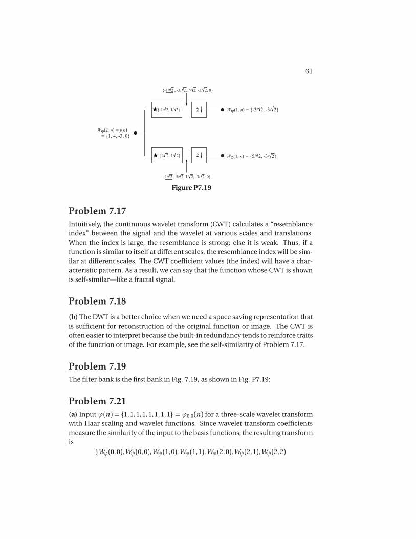
61
2
2
Wϕ(2, n) = f(n) = {1, 4, -3, 0}
Wϕ(1, n) = {5/ 2, -3/ 2}
Wψ(1, n) = {-3/ 2, -3/ 2}{-1/ 2, 1/ 2}
{1/ 2, 1/ 2}
{-1/ 2 , -3/ 2, 7/ 2, -3/ 2, 0}
{1/ 2 , 5/ 2, 1/ 2, -3/ 2, 0}
�
�
Figure P7.19
Problem 7.17Intuitively, the continuous wavelet transform (CWT) calculates a “resemblanceindex” between the signal and the wavelet at various scales and translations.When the index is large, the resemblance is strong; else it is weak. Thus, if afunction is similar to itself at different scales, the resemblance index will be sim-ilar at different scales. The CWT coefficient values (the index) will have a char-acteristic pattern. As a result, we can say that the function whose CWT is shownis self-similar—like a fractal signal.
Problem 7.18
(b) The DWT is a better choice when we need a space saving representation thatis sufficient for reconstruction of the original function or image. The CWT isoften easier to interpret because the built-in redundancy tends to reinforce traitsof the function or image. For example, see the self-similarity of Problem 7.17.
Problem 7.19The filter bank is the first bank in Fig. 7.19, as shown in Fig. P7.19:
Problem 7.21(a) Input ϕ(n ) = {1,1,1,1,1,1,1,1} = ϕ0,0(n ) for a three-scale wavelet transformwith Haar scaling and wavelet functions. Since wavelet transform coefficientsmeasure the similarity of the input to the basis functions, the resulting transformis
{Wϕ(0,0),Wψ(0,0),Wψ(1,0),Wψ(1,1),Wψ(2,0),Wψ(2,1),Wψ(2,2)

62 CHAPTER 7. PROBLEM SOLUTIONS
Wψ(2,3)}= {2�2,0,0,0,0,0,0,0}.The Wϕ(0,0) term can be computed using Eq. (7.3-5) with j0 = k = 0.
Problem 7.22They are both multi-resolution representations that employ a single reduced-resolution approximation image and a series of “difference” images. For theFWT, these “difference” images are the transform detail coefficients; for the pyra-mid, they are the prediction residuals.
To construct the approximation pyramid that corresponds to the transformin Fig. 7.10(a), we will use the F W T−1 2-d synthesis bank of Fig. 7.24(c). First,place the 64× 64 approximation “coefficients” from Fig. 7.10(a) at the top of thepyramid being constructed. Then use it, along with 64× 64 horizontal, vertical,and diagonal detail coefficients from the upper-left of Fig. 7.10(a), to drive thefilter bank inputs in Fig. 7.24(c). The output will be a 128× 128 approximationof the original image and should be used as the next level of the approximationpyramid. The 128×128 approximation is then used with the three 128×128 de-tail coefficient images in the upper 1/4 of the transform in Fig. 7.10(a) to drivethe synthesis filter bank in Fig. 7.24(c) a second time—producing a 256×256 ap-proximation that is placed as the next level of the approximation pyramid. Thisprocess is then repeated a third time to recover the 512 × 512 original image,which is placed at the bottom of the approximation pyramid. Thus, the approx-imation pyramid would have 4 levels.
Problem 7.24As can be seen in the sequence of images that are shown, the DWT is not shiftinvariant. If the input is shifted, the transform changes. Since all original imagesin the problem are 128× 128, they become the Wϕ(7,m ,n ) inputs for the FWTcomputation process. The filter bank of Fig. 7.24(a) can be used with j + 1= 7.For a single scale transform, transform coefficients Wϕ(6,m ,n ) and W i
ψ (6,m ,n )for i = H ,V,D are generated. With Haar wavelets, the transformation processsubdivides the image into non-overlapping 2× 2 blocks and computes 2-pointaverages and differences (per the scaling and wavelet vectors). Thus, there areno horizontal, vertical, or diagonal detail coefficients in the first two transformsshown; the input images are constant in all 2× 2 blocks (so all differences are0). If the original image is shifted by one pixel, detail coefficients are generatedsince there are then 2×2 areas that are not constant. This is the case in the thirdtransform shown.

NOTICE This manual is intended for your personal use only. Copying, printing, posting, or any form of printed or electronic distribution of any part of this manual constitutes a violation of copyright law. As a security measure, this manual was encrypted during download with the serial number of your book, and with your personal information. Any printed or electronic copies of this file will bear that encryption, which will tie the copy to you. Please help us defeat piracy of intellectual property, one of the principal reasons for the increase in the cost of books. -------------------------------

Chapter 8
Problem Solutions
Problem 8.4
(a) Table P8.4 shows the starting intensity values, their 8-bit codes, the IGS sumused in each step, the 4-bit IGS code and its equivalent decoded value (thedecimal equivalent of the IGS code multiplied by 16), the error between thedecoded IGS intensities and the input values, and the squared error.
(b) Using Eq. (8.1-10) and the squared error values from Table P8.4, the rms erroris
er m s =
&1
8(144+ 25+ 49+ 16+ 16+ 169+ 64+ 9)
=
&1
8(492)
= 7.84
or about 7.8 intensity levels. From Eq. (8.1-11), the signal-to-noise ratio is
SN Rm s =962+ 1442+ 1282+ 2402+ 1762+ 1602+ 642+ 962
492
=173824
492� 353.
63
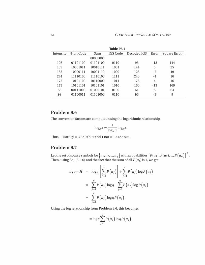
64 CHAPTER 8. PROBLEM SOLUTIONS
Table P8.4Intensity 8-bit Code Sum IGS Code Decoded IGS Error Square Error
00000000108 01101100 01101100 0110 96 -12 144139 10001011 10010111 1001 144 5 25135 10000111 10001110 1000 128 -7 49244 11110100 11110100 1111 240 -4 16172 10101100 10110000 1011 176 4 16173 10101101 10101101 1010 160 -13 16956 00111000 01000101 0100 64 8 6499 01100011 01101000 0110 96 -3 9
Problem 8.6The conversion factors are computed using the logarithmic relationship
loga x =1
logb alogb x .
Thus, 1 Hartley= 3.3219 bits and 1 nat= 1.4427 bits.
Problem 8.7
Let the set of source symbols be-
a 1,a 2, ...,aq
.with probabilities
�P (a 1) ,P (a 2) , ...,P
�aq
� T.
Then, using Eq. (8.1-6) and the fact that the sum of all P (a i ) is 1, we get
logq −H = logq
⎡⎢⎣
q∑j=1
P�
a j
�⎤⎥⎦+q∑
j=1
P�
a j
�log P
�a j
�
=q∑
j=1
P�
a j
�logq +
q∑j=1
P�
a j
�log P
�a j
�
=q∑
j=1
P�
a j
�logqP
�a j
�.
Using the log relationship from Problem 8.6, this becomes
= log eq∑
j=1
P�
a j
�lnqP
�a j
�.
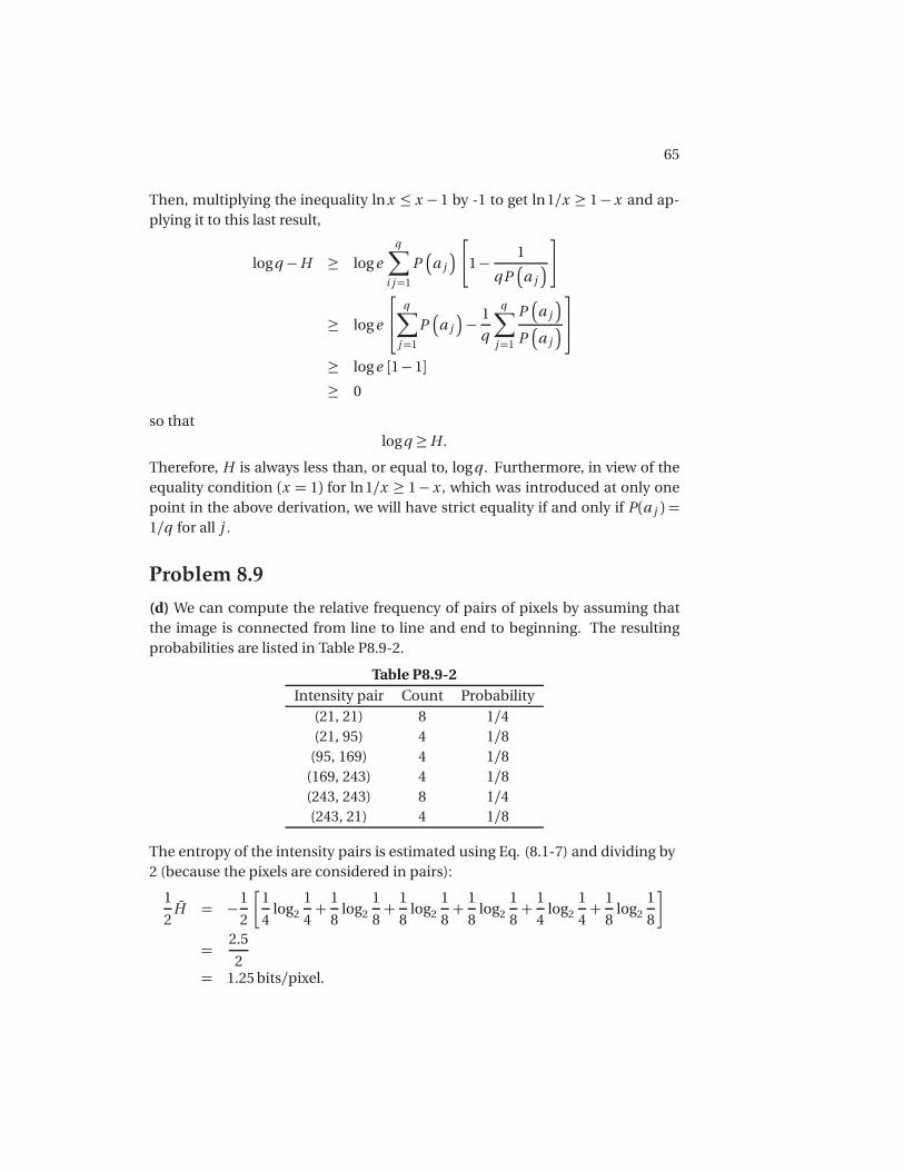
65
Then, multiplying the inequality lnx ≤ x − 1 by -1 to get ln1/x ≥ 1− x and ap-plying it to this last result,
logq −H ≥ log eq∑
i j=1
P�
a j
�⎡⎣1− 1
qP�
a j
�⎤⎦
≥ log e
⎡⎢⎣
q∑j=1
P�
a j
�− 1
q
q∑j=1
P�
a j
�P�
a j
�⎤⎥⎦
≥ log e [1− 1]
≥ 0
so thatlogq ≥H .
Therefore, H is always less than, or equal to, logq . Furthermore, in view of theequality condition (x = 1) for ln 1/x ≥ 1− x , which was introduced at only onepoint in the above derivation, we will have strict equality if and only if P(a j ) =1/q for all j .
Problem 8.9
(d) We can compute the relative frequency of pairs of pixels by assuming thatthe image is connected from line to line and end to beginning. The resultingprobabilities are listed in Table P8.9-2.
Table P8.9-2Intensity pair Count Probability
(21, 21) 8 1/4(21, 95) 4 1/8
(95, 169) 4 1/8(169, 243) 4 1/8(243, 243) 8 1/4(243, 21) 4 1/8
The entropy of the intensity pairs is estimated using Eq. (8.1-7) and dividing by2 (because the pixels are considered in pairs):
1
2H = −1
2
�1
4log2
1
4+
1
8log2
1
8+
1
8log2
1
8+
1
8log2
1
8+
1
4log2
1
4+
1
8log2
1
8
�
=2.5
2= 1.25 bits/pixel.

66 CHAPTER 8. PROBLEM SOLUTIONS
The difference between this value and the entropy in (a) tells us that a mappingcan be created to eliminate (1.811− 1.25) = 0.56 bits/pixel of spatialredundancy.
Problem 8.15To decode G k
e x p (n ):
1. Count the number of 1s in a left-to-right scan of a concatenated G ke x p (n )
bit sequence before reaching the first 0, and let i be the number of 1scounted.
2. Get the k+i bits following the 0 identified in step 1 and let d be its decimalequivalent.
3. The decoded integer is then
d +i−1∑j=0
2j+k .
For example, to decode the first G 2e x p (n ) code in the bit stream 10111011..., let
i = 1, the number of 1s in a left-to-right scan of the bit stream before finding thefirst 0. Get the 2+ 1 = 3 bits following the 0, that is, 111 so d = 7. The decodedinteger is then
7+1−1∑j=0
2j+2= 7+ 22 = 11.
Repeat the process for the next code word, which begins with the bit sequence011...
Problem 8.18The arithmetic decoding process is the reverse of the encoding procedure. Startby dividing the [0, 1) interval according to the symbol probabilities. This isshown in Table P8.18. The decoder immediately knows the message 0.23355begins with an “e”, since the coded message lies in the interval [0.2, 0.5). Thismakes it clear that the second symbol is an “a”, which narrows the interval to[0.2, 0.26). To further see this, divide the interval [0.2, 0.5) according to the sym-bol probabilities. Proceeding like this, which is the same procedure used to codethe message, we get “eaii!”.
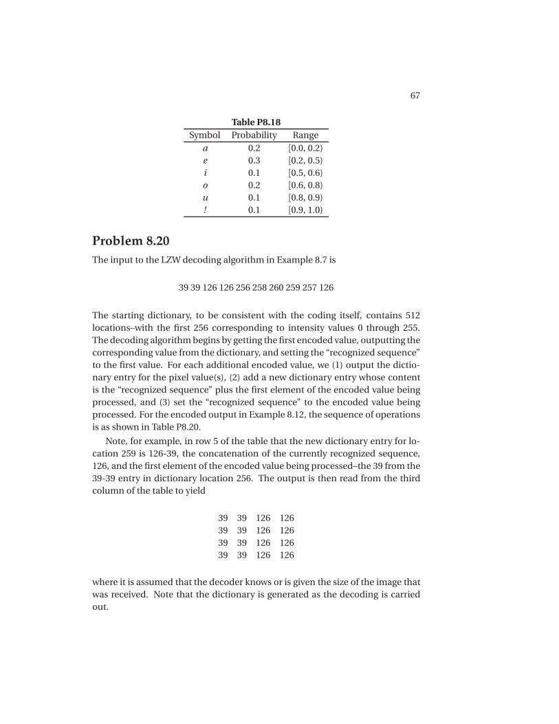
67
Table P8.18Symbol Probability Range
a 0.2 [0.0, 0.2)e 0.3 [0.2, 0.5)i 0.1 [0.5, 0.6)o 0.2 [0.6, 0.8)u 0.1 [0.8, 0.9)! 0.1 [0.9, 1.0)
Problem 8.20The input to the LZW decoding algorithm in Example 8.7 is
39 39 126 126 256 258 260 259 257 126
The starting dictionary, to be consistent with the coding itself, contains 512locations–with the first 256 corresponding to intensity values 0 through 255.The decoding algorithm begins by getting the first encoded value, outputting thecorresponding value from the dictionary, and setting the “recognized sequence”to the first value. For each additional encoded value, we (1) output the dictio-nary entry for the pixel value(s), (2) add a new dictionary entry whose contentis the “recognized sequence” plus the first element of the encoded value beingprocessed, and (3) set the “recognized sequence” to the encoded value beingprocessed. For the encoded output in Example 8.12, the sequence of operationsis as shown in Table P8.20.
Note, for example, in row 5 of the table that the new dictionary entry for lo-cation 259 is 126-39, the concatenation of the currently recognized sequence,126, and the first element of the encoded value being processed–the 39 from the39-39 entry in dictionary location 256. The output is then read from the thirdcolumn of the table to yield
39 39 126 12639 39 126 12639 39 126 12639 39 126 126
where it is assumed that the decoder knows or is given the size of the image thatwas received. Note that the dictionary is generated as the decoding is carriedout.

68 CHAPTER 8. PROBLEM SOLUTIONS
Table P8.20Recognized Encoded Value Pixels Dict. Address Dict. Entry
39 3939 39 39 256 39-3939 126 126 257 39-126
126 126 126 258 126-126126 256 39-39 259 126-39256 258 126-126 260 39-39-126258 260 39-39-126 261 126-126-39260 259 126-39 262 39-39-126-126259 257 39-126 263 126-39-39257 126 126 264 39-126-126
Problem 8.24(a) - (b) Following the procedure outlined in Section 8.2.8, we obtain the resultsshown in Table P8.24.
Table P8.24DC Coefficient Difference Two’s Complement Value Code
-7 1...1001 00000-6 1...1010 00001-5 1...1011 00010-4 1...1100 000114 0...0100 001005 0...0101 001016 0...0110 001107 0...0111 00111
Problem 8.27The appropriate MPEG decoder is shown in Fig. P8.27.

69
Inverse Mapper(e.g., DCT-1)
InverseQuantizer
VariableLength
Decoder
DecodedImage
Macroblock
VariableLength
DecoderMotion Estimatorand Compensator
+EncodedMacroblock
EncodedMotionVector
Figure P8.27
Problem 8.29The derivation proceeds by substituting the uniform probability function intoEqs. (8.2-57) - (8.2-59) and solving the resulting simultaneous equations withL = 4. Equation (8.2-58) yields
s0 = 0s1 = 1
2 (t1+ t2)s2 =∞.
Substituting these values into the integrals defined by Eq. (8.2-57), we get twoequations. The first is (assuming s1 ≤A)
∫ s1
s0
(s − t1)p (s )d s = 0
1
2A
∫ 12 (t1+t2)
0
(s − t1)d s =s 2
2− t1s
����12 (t1+ t2)0
= 0
(t1+ t2)2− 4t1 (t1+ t2) = 0
(t1+ t2) (t2− 3t1) = 0
so
t1 = −t2
t2 = 3t1.
The first of these relations does not make sense since both t1 and t2 must be pos-itive. The second relationship is a valid one. The second integral yields (notingthat s1 is less than A so the integral from A to∞ is 0 by the definition of p (s ))

70 CHAPTER 8. PROBLEM SOLUTIONS
∫ s2
s1
(s − t2)p (s )d s = 0
1
2A
∫ A
12 (t1+t2)
(s − t2)d s =s 2
2− t2s
���� A12 (t1+ t2)
= 0
4A2− 8At2− (t1+ t2)2− 4t2 (t1+ t2) = 0.
Substituting t2 = 3t1 from the first integral simplification into this result, we get
8t 21 − 6At1+A2 = 0�
t1− A
2
�(8t1− 2A) = 0
t1 =A
2
t1 =A
4.
Back substituting these values of t1, we find the corresponding t2 and s1 values:
t2 = 3A2 and s1 =A for t1 = A
2t2 = 3A
4 and s1 = A2 for t1 = A
4 .
Because s1 = A is not a real solution (the second integral equation would thenbe evaluated from A to A, yielding 0 or no equation), the solution is given by thesecond. That is,
s0 = 0 s1 = A2 s2 =∞
t1 = A4 t2 = 3A
4 .
Problem 8.34A variety of methods for inserting invisible watermarks into the DFT coefficientsof an image have been reported in the literature. Here is a simplified outline ofone in which watermark insertion is done as follows:
1. Create a watermark by generating a P-element pseudo-random sequenceof numbers, ω1,ω2, ...,ωP , taken from a Gaussian distribution with zeromean and unit variance.
2. Compute the DFT of the image to be watermarked. We assume that thetransform has not been centered by pre-multiplying the image by (−1)x+y .

71
3. Choose P2 coefficients from each of the four quadrants of the DFT in the
middle frequency range. This is easily accomplished by choosing coeffi-cients in the order shown in Fig. P8.34 and skipping the first K coefficients(the low frequency coefficients) in each quadrant.
4. Insert the first half of the watermark into the chosen DFT coefficients, ci
for 1≤ i ≤ P2 , in quadrants I and III of the DFT using
c ′i = ci (1+αωi )
5. Insert the second half of the watermark into the chosen DFT coefficientsof quadrants II and IV of the DFT in a similar manner. Note that this pro-cess maintains the symmetry of the transform of a real-valued image. Inaddition, constant α determines the strength of the inserted watermark.
6. Compute the inverse DFT with the watermarked coefficients replacing theunmarked coefficients.
Watermark extraction is performed as follows:
1. Locate the DFT coefficients containing the watermark by following the in-sertion process in the embedding algorithm.
2. Compute the watermark ω1,ω2, ...,ωP using
ωi = c i − ci
3. Compute the correlation betweenω and ωand compare to a pre-determinedthreshold T to determine if the mark is present.
This is some blan text to move figure to top of page.This is some blan text to move figure to top of page.This is some blan text to move figure to top of page.This is some blan text to move figure to top of page.This is some blan text to move figure to top of page.This is some blan text to move figure to top of page.This is some blan text to move figure to top of page.This is some blan text to move figure to top of page.This is some blan text to move figure to top of page.

72 CHAPTER 8. PROBLEM SOLUTIONS
II I
III IV
Figure P8.34
This is some blan text to move figure to top of page.This is some blan text to move figure to top of page.This is some blan text to move figure to top of page.This is some blan text to move figure to top of page.This is some blan text to move figure to top of page.

NOTICE This manual is intended for your personal use only. Copying, printing, posting, or any form of printed or electronic distribution of any part of this manual constitutes a violation of copyright law. As a security measure, this manual was encrypted during download with the serial number of your book, and with your personal information. Any printed or electronic copies of this file will bear that encryption, which will tie the copy to you. Please help us defeat piracy of intellectual property, one of the principal reasons for the increase in the cost of books. -------------------------------

Chapter 9
Problem Solutions
Problem 9.2(a) With reference to the discussion in Section 2.5.2, m-connectivity is used toavoid multiple paths that are inherent in 8-connectivity. In one-pixel-thick, fullyconnected boundaries, these multiple paths manifest themselves in the four ba-sic patterns shown in Fig. P9.2(a). The solution to the problem is to use the hit-or-miss transform to detect the patterns and then to change the center pixel to0, thus eliminating the multiple paths. A basic sequence of morphological stepsto accomplish this is as follows:
X1 = A � B 1
Y1 = A ∩X c1
X2 = Y1� B 2
Y2 = Y1 ∩X c2
X3 = Y2� B 3
Y3 = Y2 ∩X c3
X4 = Y3� B 4
Y4 = Y3 ∩X c4
where A is the input image containing the boundary.
Problem 9.4(a) Erosion is set intersection. The intersection of two convex sets is convex also.
(b) See Fig. P9.4(a). Keep in mind that the digital sets in question are the largerblack dots. The lines are shown for convenience in visualizing what the continu-
73

74 CHAPTER 9. PROBLEM SOLUTIONS
Figure P9.2
Figure P9.4
ous sets would be, they are not part of the sets being considered here. The resultof dilation in this case is not convex because the center point is not in the set.
Problem 9.5Refer to Fig. P9.5. The center of each structuring element is shown as a blackdot.
(a) This solution was obtained by eroding the original set (shown dashed) withthe structuring element shown (note that the origin is at the bottom, right).
(b) This solution was obtained by eroding the original set with the tall rectangu-lar structuring element shown.
(c) This solution was obtained by first eroding the image shown down to twovertical lines using the rectangular structuring element (note that this elementsis slightly taller than the center section of the “U” figure). This result was thendilated with the circular structuring element.
(d) This solution was obtained by first dilating the original set with the large diskshown. The dilated image was eroded with a disk whose diameter was equal toone-half the diameter of the disk used for dilation.
Problem 9.7(a) The dilated image will grow without bound.
(b) A one-element set (i.e., a one-pixel image).
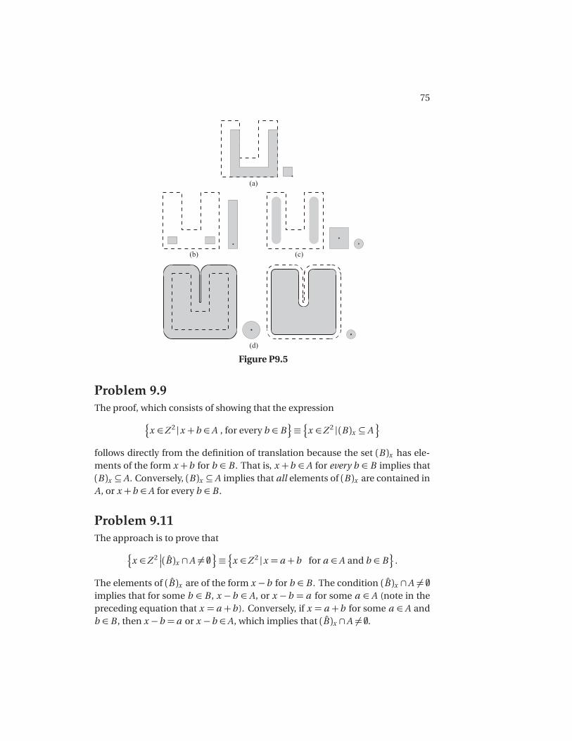
75
(a)
(b) (c)
(d)
Figure P9.5
Problem 9.9The proof, which consists of showing that the expression-
x ∈Z 2 |x +b ∈ A , for every b ∈ B.≡ -x ∈Z 2 | (B )x ⊆ A
.follows directly from the definition of translation because the set (B )x has ele-ments of the form x +b for b ∈ B . That is, x +b ∈ A for every b ∈ B implies that(B )x ⊆A. Conversely, (B )x ⊆ A implies that all elements of (B )x are contained inA, or x +b ∈ A for every b ∈ B .
Problem 9.11The approach is to prove that-
x ∈Z 2��(B )x ∩A �= �.≡ -x ∈Z 2 |x = a +b for a ∈ A and b ∈ B
..
The elements of (B )x are of the form x −b for b ∈ B . The condition (B )x ∩A �= �implies that for some b ∈ B , x −b ∈ A, or x −b = a for some a ∈ A (note in thepreceding equation that x = a +b ). Conversely, if x = a +b for some a ∈ A andb ∈ B , then x −b = a or x −b ∈ A, which implies that (B )x ∩A �= �.

76 CHAPTER 9. PROBLEM SOLUTIONS
Problem 9.14Starting with the definition of closing,
(A • B )c = [(A ⊕ B )� B ]c
= (A ⊕ B )c ⊕ B
= (Ac � B )⊕ B
= Ac ◦ B .
The proof of the other duality property follows a similar approach.
Problem 9.15(a) Erosion of a set A by B is defined as the set of all values of translates, z , of Bsuch that (B )z is contained in A. If the origin of B is contained in B , then the setof points describing the erosion is simply all the possible locations of the originof B such that (B )z is contained in A. Then it follows from this interpretation(and the definition of erosion) that erosion of A by B is a subset of A. Similarly,dilation of a set C by B is the set of all locations of the origin of B such that theintersection of C and (B )z is not empty. If the origin of B is contained in B , thisimplies that C is a subset of the dilation of C by B . From Eq. (9.3-1), we knowthat A ◦ B = (A � B )⊕ B . Let C denote the erosion of A by B . It was alreadyestablished that C is a subset of A. From the preceding discussion, we know alsothat C is a subset of the dilation of C by B . But C is a subset of A, so the openingof A by B (the erosion of A by B followed by a dilation of the result) is a subset ofA.
Problem 9.18It was possible to reconstruct the three large squares to their original size be-cause they were not completely eroded and the geometry of the objects andstructuring element was the same (i.e., they were squares). This also would havebeen true if the objects and structuring elements were rectangular. However, acomplete reconstruction, for instance, by dilating a rectangle that was partiallyeroded by a circle, would not be possible.
Problem 9.20The key difference between the Lake and the other two features is that the for-mer forms a closed contour. Assuming that the shapes are processed one at atime, a basic two-step approach for differentiating between the three shapes isas follows:

77
Figure P9.22
Step 1. Apply an end-point detector to the object. If no end points are found,the object is a Lake. Otherwise it is a Bay or a Line.
Step 2. There are numerous ways to differentiate between a Bay and a Line.One of the simplest is to determine a line joining the two end points of the ob-ject. If the AND of the object and this line contains only two points, the fig-ure is a Bay. Otherwise it is a Line. There are pathological cases in which thistest will fail, and additional ”intelligence” needs to be built into the process, butthese pathological cases become less probable with increasing resolution of thethinned figures.
Problem 9.22(a) With reference to the example shown in Fig. P9.22, the boundary that re-sults from using the structuring element in Fig. 9.15(c) generally forms an 8-connected path (leftmost figure), whereas the boundary resulting from the struc-turing element in Fig. 9.13(b) forms a 4-connected path (rightmost figure).
Problem 9.23(a) If the spheres are not allowed to touch, the solution of the problem starts bydetermining which points are background (black) points. To do this, we pick ablack point on the boundary of the image and determine all black points con-nected to it using a connected component algorithm(Section 9.5.3). These con-
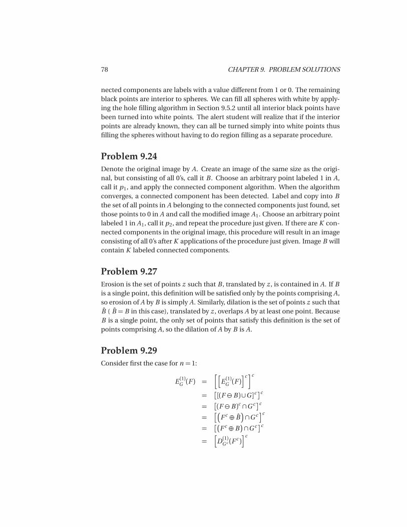
78 CHAPTER 9. PROBLEM SOLUTIONS
nected components are labels with a value different from 1 or 0. The remainingblack points are interior to spheres. We can fill all spheres with white by apply-ing the hole filling algorithm in Section 9.5.2 until all interior black points havebeen turned into white points. The alert student will realize that if the interiorpoints are already known, they can all be turned simply into white points thusfilling the spheres without having to do region filling as a separate procedure.
Problem 9.24Denote the original image by A. Create an image of the same size as the origi-nal, but consisting of all 0’s, call it B . Choose an arbitrary point labeled 1 in A,call it p1, and apply the connected component algorithm. When the algorithmconverges, a connected component has been detected. Label and copy into Bthe set of all points in A belonging to the connected components just found, setthose points to 0 in A and call the modified image A1. Choose an arbitrary pointlabeled 1 in A1, call it p2, and repeat the procedure just given. If there are K con-nected components in the original image, this procedure will result in an imageconsisting of all 0’s after K applications of the procedure just given. Image B willcontain K labeled connected components.
Problem 9.27Erosion is the set of points z such that B , translated by z , is contained in A. If Bis a single point, this definition will be satisfied only by the points comprising A,so erosion of A by B is simply A. Similarly, dilation is the set of points z such thatB ( B = B in this case), translated by z , overlaps A by at least one point. BecauseB is a single point, the only set of points that satisfy this definition is the set ofpoints comprising A, so the dilation of A by B is A.
Problem 9.29Consider first the case for n = 1:
E (1)G (F ) = "
E (1)G (F )#c!c
=�[(F � B )∪G ]c
c
=�(F � B )c ∩G c c
=��
F c ⊕ B�∩G c
c
=��
F c ⊕ B�∩G c c
="
D (1)G c (F c )#c

79
where the third step follows from DeMorgan’s law, (A ∪ B )c =Ac ∩ B c , the fourthstep follows from the duality property of erosion and dilation (see Section 9.2.3),the fifth step follows from the symmetry of the SE, and the last step follows fromthe definition of geodesic dilation. The next step, E (2)G (F ), would involve thegeodesic erosion of the above result. But that result is simply a set, so we couldobtain it in terms of dilation. That is, we would complement the result just men-tioned, complement G , compute the geodesic dilation of size 1 of the two, andcomplement the result. Continuing in this manner we conclude that
E (n )G =
D (1)G c
�"E (n−1)
G (F )#c�!c
="
D (1)G c
�D (n−1)
G c
�F c��#c
.
Similarly,
D (1)G (F ) = "
D (1)G (F )#c!c
=�[(F ⊕ B )∩G ]c
c
=�(F ⊕ B )c ∪G c c
=��
F c � B�∪G c
c
=��
F c � B�∪G c c
="
E (1)G c (F c )#c
.
As before,
D (n )G =
E (1)G c
�"D (n−1)
G (F )#c�!c
="
E (1)G c
�E (n−1)
G c
�F c��#c
.
Problem 9.31(a) Consider the case when n = 2
[(F � 2B )]c = [(F � B )� B ]c
= (F � B )c ⊕ B
=�
F c ⊕ B�⊕ B
=�
F c ⊕ 2B�

80 CHAPTER 9. PROBLEM SOLUTIONS
where the second and third lines follow from the duality property in Eq. (9.2-5).For an arbitrary number of erosions,
[(F �n B )]c = [(F � (n − 1)B )� B ]c
= [(F � (n − 1)B )]c ⊕ B
which, when expanded, will yield [(F �n B )]c = F c ⊕n B .
(b) Proved in a similar manner.
Problem 9.33(a) From Eq. (9.6-1),
�f �b
�c =�
min(s ,t )∈b
f (x + s ,y + t )
��c
=�− max(s ,t )∈b
− f (x + s ,y + t )��c
= max(s ,t )∈b
− f (x + s ,y + t )�
= − f ⊕ b
= f c ⊕ b .
The second step follows from the definition of the complement of a gray-scale
function; that is, the minimum of a set of numbers is equal to the negative ofthe maximum of the negative of those numbers. The third step follows fromthe definition of the complement. The fourth step follows from the definition ofgray-scale dilation in Eq. (9.6-2), using the fact that b (x ,y ) = b (−x − y ). The laststep follows from the definition of the complement, − f = f c . The other dualityproperty is proved in a similar manner.
(c) We prove the first duality property. Start with the a geodesic dilation of size1:
D (1)g
�f�=
"D (1)g
�f�#c!c
=��(f ⊕b )∧ g
c c
=��−�−(f ⊕b )∨−g
�c c
=�−(f ⊕b )∨−g
c
=�(f ⊕b )c ∨ g c c
=�(f c �b )∨ g c c
="
E (1)g c
�f c �#c
.

81
Figure P9.35
The second step follows from the definition of geodesic dilation. The third stepfollows from the fact that the point-wise minimum of two sets of numbers is thenegative of the point-wise maximum of the two numbers. The fourth and fifthsteps follow from the definition of the complement. The sixth step follows fromthe duality of dilation and erosion (we used the given fact that b = b ). The laststep follows from the definition of geodesic erosion.
The next step in the iteration, D (2)g�
f�
, would involve the geodesic dilation ofsize 1 of the preceding result. But that result is simply a set, so we could obtainit in terms of erosion. That is, we would complement the result just mentioned,complement g , compute the geodesic erosion of the two, and complement theresult. Continuing in this manner we conclude that
D (n )g (f ) ="
E (1)g c
�E (n−1)
g c
�f c ��#c
.
The other property is proved in a similar way.
Problem 9.35(a) The noise spikes are of the general form shown in Fig. P9.35(a), with otherpossibilities in between. The amplitude is irrelevant in this case; only the shapeof the noise spikes is of interest. To remove these spikes we perform an openingwith a cylindrical structuring element of radius greater than Rmax, as shown inFig. P9.35(b). Note that the shape of the structuring element is matched to theknown shape of the noise spikes.

82 CHAPTER 9. PROBLEM SOLUTIONS
Problem 9.36(a) Color the image border pixels the same color as the particles (white). Callthe resulting set of border pixels B . Apply the connected component algorithm(Section 9.5.3). All connected components that contain elements from B areparticles that have merged with the border of the image.

NOTICE This manual is intended for your personal use only. Copying, printing, posting, or any form of printed or electronic distribution of any part of this manual constitutes a violation of copyright law. As a security measure, this manual was encrypted during download with the serial number of your book, and with your personal information. Any printed or electronic copies of this file will bear that encryption, which will tie the copy to you. Please help us defeat piracy of intellectual property, one of the principal reasons for the increase in the cost of books. -------------------------------

Chapter 10
Problem Solutions
Problem 10.1Expand f (x +Δx ) into a Taylor series about x :
f (x +Δx ) = f (x )+Δx f ′(x )+ (Δx )2!
f ′′(x )+ · · ·
The increment in the spatial variable x is defined in Section 2.4.2 to be 1, so bylettingΔx = 1 and keeping only the linear terms we obtain the result
f ′(x ) = f (x + 1)− f (x )
which agrees with Eq. (10.2-1).
Problem 10.2The masks would have the coefficients shown in Fig. P10.2. Each mask wouldyield a value of 0 when centered on a pixel of an unbroken 3-pixel segment ori-ented in the direction favored by that mask. Conversely, the response would bea +2 when a mask is centered on a one-pixel gap in a 3-pixel segment orientedin the direction favored by that mask.
Problem 10.4(a) The lines were thicker than the width of the line detector masks. Thus, when,for example, a mask was centered on the line it “saw” a constant area and gave aresponse of 0.
83
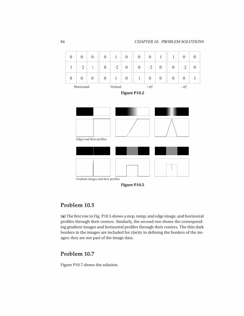
84 CHAPTER 10. PROBLEM SOLUTIONS
Figure P10.2
Edges and their profiles
Gradient images and their profiles
Figure P10.5
Problem 10.5
(a) The first row in Fig. P10.5 shows a step, ramp, and edge image, and horizontalprofiles through their centers. Similarly, the second row shows the correspond-ing gradient images and horizontal profiles through their centers. The thin darkborders in the images are included for clarity in defining the borders of the im-ages; they are not part of the image data.
Problem 10.7
Figure P10.7 shows the solution.
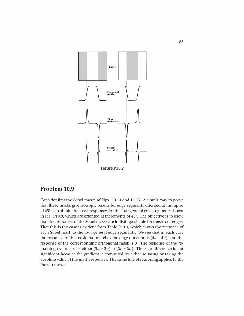
85
Figure P10.7
Problem 10.9
Consider first the Sobel masks of Figs. 10.14 and 10.15. A simple way to provethat these masks give isotropic results for edge segments oriented at multiplesof 45◦ is to obtain the mask responses for the four general edge segments shownin Fig. P10.9, which are oriented at increments of 45◦. The objective is to showthat the responses of the Sobel masks are indistinguishable for these four edges.That this is the case is evident from Table P10.9, which shows the response ofeach Sobel mask to the four general edge segments. We see that in each casethe response of the mask that matches the edge direction is (4a − 4b ), and theresponse of the corresponding orthogonal mask is 0. The response of the re-maining two masks is either (3a − 3b ) or (3b − 3a ). The sign difference is notsignificant because the gradient is computed by either squaring or taking theabsolute value of the mask responses. The same line of reasoning applies to thePrewitt masks.

86 CHAPTER 10. PROBLEM SOLUTIONS
Figure P10.9
Table P10.9Edge Horizontal Vertical +45◦ −45◦
direction Sobel (g x ) Sobel (g y ) Sobel (g 45) Sobel (g−45)Horizontal 4a − 4b 0 3a − 3b 3b − 3a
Vertical 0 4a − 4b 3a − 3b 3a − 3b+45◦ 3a − 3b 3a − 3b 4a − 4b 0−45◦ 3b − 3a 3a − 3b 0 4a − 4b
Problem 10.11(a) The operators are as follows (negative numbers are shown underlined):
111 110 101 01 1 1 11 1 10 1 01 011
000 101 101 101 000 1 01 101 101
11 1 01 1 101 110 111 011 101 11 0
Problem 10.13(a) The local average at a point (x ,y ) in an image is given by
f (x ,y ) =1
n 2
∑z i∈Sx y
z i
where Sx y is the region in the image encompassed by the n ×n averaging maskwhen it is centered at (x ,y ) and the z i are the intensities of the image pixels inthat region. The partial
∂ f /∂ x = f (x + 1,y )− f (x ,y )
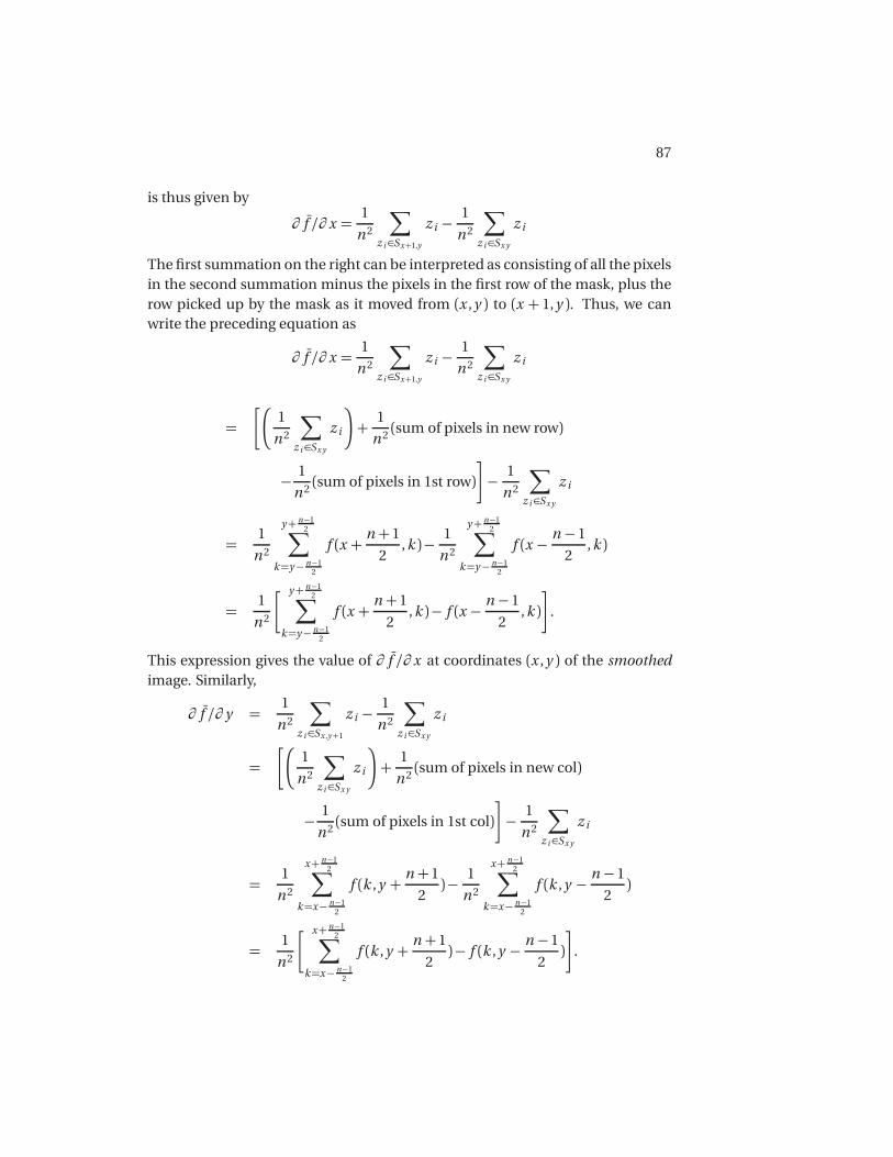
87
is thus given by
∂ f /∂ x =1
n 2
∑z i∈Sx+1,y
z i − 1
n 2
∑z i∈Sx y
z i
The first summation on the right can be interpreted as consisting of all the pixelsin the second summation minus the pixels in the first row of the mask, plus therow picked up by the mask as it moved from (x ,y ) to (x + 1,y ). Thus, we canwrite the preceding equation as
∂ f /∂ x =1
n 2
∑z i∈Sx+1,y
z i − 1
n 2
∑z i∈Sx y
z i
=
'+1
n 2
∑z i∈Sx y
z i
,+
1
n 2 (sum of pixels in new row)
− 1
n 2(sum of pixels in 1st row)
(− 1
n 2
∑z i∈Sx y
z i
=1
n 2
y+ n−12∑
k=y− n−12
f (x +n + 1
2,k )− 1
n 2
y+ n−12∑
k=y− n−12
f (x − n − 1
2,k )
=1
n 2
' y+ n−12∑
k=y− n−12
f (x +n + 1
2,k )− f (x − n − 1
2,k )
(.
This expression gives the value of ∂ f /∂ x at coordinates (x ,y ) of the smoothedimage. Similarly,
∂ f /∂ y =1
n 2
∑z i∈Sx ,y+1
z i − 1
n 2
∑z i∈Sx y
z i
=
'+1
n 2
∑z i∈Sx y
z i
,+
1
n 2(sum of pixels in new col)
− 1
n 2 (sum of pixels in 1st col)
(− 1
n 2
∑z i∈Sx y
z i
=1
n 2
x+ n−12∑
k=x− n−12
f (k ,y +n + 1
2)− 1
n 2
x+ n−12∑
k=x− n−12
f (k ,y − n − 1
2)
=1
n 2
' x+ n−12∑
k=x− n−12
f (k ,y +n + 1
2)− f (k ,y − n − 1
2)
(.

88 CHAPTER 10. PROBLEM SOLUTIONS
The edge magnitude image corresponding to the smoothed image f (x ,y ) is thengiven by
M (x ,y ) =$(∂ f /∂ x )2+(∂ f /∂ y )2.
Problem 10.14
(a) We proceeed as follows
Average�∇2G (x ,y )
=
∫ ∞−∞
∫ ∞−∞∇2G (x ,y )d x d y
=
∫ ∞−∞
∫ ∞−∞
�x 2+ y 2− 2σ2
σ4
�e−
x 2+y 2
2σ2 d x d y
=1
σ4
∫ ∞−∞
x 2e−x 2
2σ2 d x
∫ ∞−∞
e−y 2
2σ2 d y
+1
σ4
∫ ∞−∞
y 2e−y 2
2σ2 d y
∫ ∞−∞
e−x 2
2σ2 d x
− 2
σ2
∫ ∞−∞
e−x 2+y 2
2σ2 d x d y
=1
σ4
��2πσ×σ2
���2πσ
�+
1
σ4
��2πσ×σ2
���2πσ
�
−2�
2πσ2�
σ2
= 4π− 4π
= 0
the fourth line follows from the fact that
variance(z ) =σ2 =1�
2πσ
∫ ∞−∞
z 2e−z 2
2σ2 d z
and1�
2πσ
∫ ∞−∞
e−z 2
2σ2 d z = 1.
Problem 10.15
(b) The answer is yes for functions that meet certain mild conditions, and ifthe zero crossing method is based on rotational operators like the LoG func-

89
tion and a threshold of 0. Geometrical properties of zero crossings in generalare explained in some detail in the paper ”On Edge Detection,” by V. Torre and T.Poggio, IEEE Trans. Pattern Analysis and Machine Intell., vol. 8, no. 2, 1986, pp.147-163. Looking up this paper and becoming familiar with the mathematicalunderpinnings of edge detection is an excellent reading assignment for graduatestudents.
Problem 10.18
(a) Equation (10.2-21) can be written in the following separable form
G (x ,y ) = e−x 2+y 2
2σ2
= e−x 2
2σ2 e−y 2
2σ2
= G (x )G (y ).
From Eq. (3.4-2) and the preceding equation, the convolution of G (x ,y ) andf (x ,y ) can be written as
G (x ,y ) f (x ,y ) =a∑
s=−a
a∑t=−a
G (s , t )f (x − s ,y − t )
=a∑
s=−a
a∑t=−a
e−s 2
2σ2 e−t 2
2σ2 f (x − s ,y − t )
=a∑
s=−a
e−s 2
2σ2
⎡⎣ a∑
t=−a
e−t 2
2σ2 f (x − s ,y − t )
⎤⎦
where a = (n − 1)/2 and n is the size of the n ×n mask obtained by samplingEq. (10.2-21). The expression inside the brackets is the 1-D convolution of theexponential term, e−t 2/2σ2 , with the rows of f (x ,y ). Then the outer summationis the convolution of e−s 2/2σ2 with the columns of the result. Stated another way,
G (x ,y ) f (x ,y ) =G (x )�G (y ) f (x ,y )
.
Problem 10.19(a) As Eq. (10.2-25) shows, the first two steps of the algorithm can be summa-rized into one equation:
g (x ,y ) =∇2[G (x ,y ) f (x ,y )].
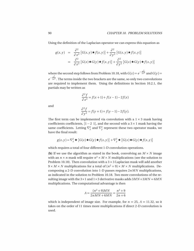
90 CHAPTER 10. PROBLEM SOLUTIONS
Using the definition of the Laplacian operator we can express this equation as
g (x ,y ) =∂ 2
∂ x 2
�G (x ,y ) f (x ,y )
+∂ 2
∂ y 2
�G (x ,y ) f (x ,y )
=∂ 2
∂ x 2
�G (x ) G (y ) f (x ,y )
+∂ 2
∂ y 2
�G (x ) G (y ) f (x ,y )
where the second step follows from Problem 10.18, with G (x ) = e−x 2
2σ2 and G (y ) =
e−y 2
2σ2 . The terms inside the two brackets are the same, so only two convolutionsare required to implement them. Using the definitions in Section 10.2.1, thepartials may be written as
∂ 2 f
∂ x 2 = f (x + 1)+ f (x − 1)− 2f (x )
and∂ 2 f
∂ y 2 = f (y + 1)+ f (y − 1)− 2f (y ).
The first term can be implemented via convolution with a 1× 3 mask havingcoefficients coefficients, [1− 2 1], and the second with a 3× 1 mask having thesame coefficients. Letting ∇2
x and ∇2y represent these two operator masks, we
have the final result:
g (x ,y ) =∇2x
�G (x ) G (y ) f (x ,y )
+∇2
y
�G (x ) G (y ) f (x ,y )
which requires a total of four different 1-D convolution operations.
(b) If we use the algorithm as stated in the book, convolving an M ×N imagewith an n ×n mask will require n 2×M ×N multiplications (see the solution toProblem 10.18). Then convolution with a 3× 3 Laplacian mask will add another9×M ×N multiplications for a total of (n 2 + 9)×M ×N multiplications. De-composing a 2-D convolution into 1-D passes requires 2nM N multiplications,as indicated in the solution to Problem 10.18. Two more convolutions of the re-sulting image with the 3×1 and 1×3 derivative masks adds 3M N+3M N = 6M Nmultiplications. The computational advantage is then
A =(n 2+ 9)M N
2nM N + 6M N=
n 2+ 9
2n + 6
which is independent of image size. For example, for n = 25, A = 11.32, so ittakes on the order of 11 times more multiplications if direct 2-D convolution isused.

91
Problem 10.21Parts (a) through (c) are shown in rows 2 through 4 of Fig. P10.21.
Problem 10.22
(b) θ = cot−1(2) = 26.6◦ and ρ = (1)sinθ = 0.45.
Problem 10.23(a) Point 1 has coordinates x = 0 and y = 0. Substituting into Eq. (10.2-38) yieldsρ = 0, which, in a plot of ρ vs. θ , is a straight line.
(b) Only the origin (0,0) would yield this result.(c) At θ =+90◦, it follows from Eq. (10.2-38) that x · (0)+ y · (1) = ρ, or y =ρ. Atθ =−90◦ , x · (0)+ y · (−1) =ρ, or−y =ρ. Thus the reflective adjacency.
Problem 10.26The essence of the algorithm is to compute at each step the mean value, m1, ofall pixels whose intensities are less than or equal to the previous threshold and,similarly, the mean value, m2, of all pixels with values that exceed the threshold.Let pi = n i/n denote the i th component of the image histogram, where n i isthe number of pixels with intensity i , and n is the total number of pixels in theimage. Valid values of i are in the range 0≤ i ≤ L− 1, where L is the number onintensities and i is an integer. The means can be computed at any step k of thealgorithm:
m1(k ) =I (k−1)∑
i=0
i pi /P(k )
where
P(k ) =I (k−1)∑
i=0
pi
and
m2(k ) =L−1∑
i=I (k−1)+1
i pi /[1−P(k )] .
The term I (k − 1) is the smallest integer less than or equal to T (k − 1), and T (0)is given. The next value of the threshold is then
T (k + 1) =1
2[m1(k )+m2(k )] .
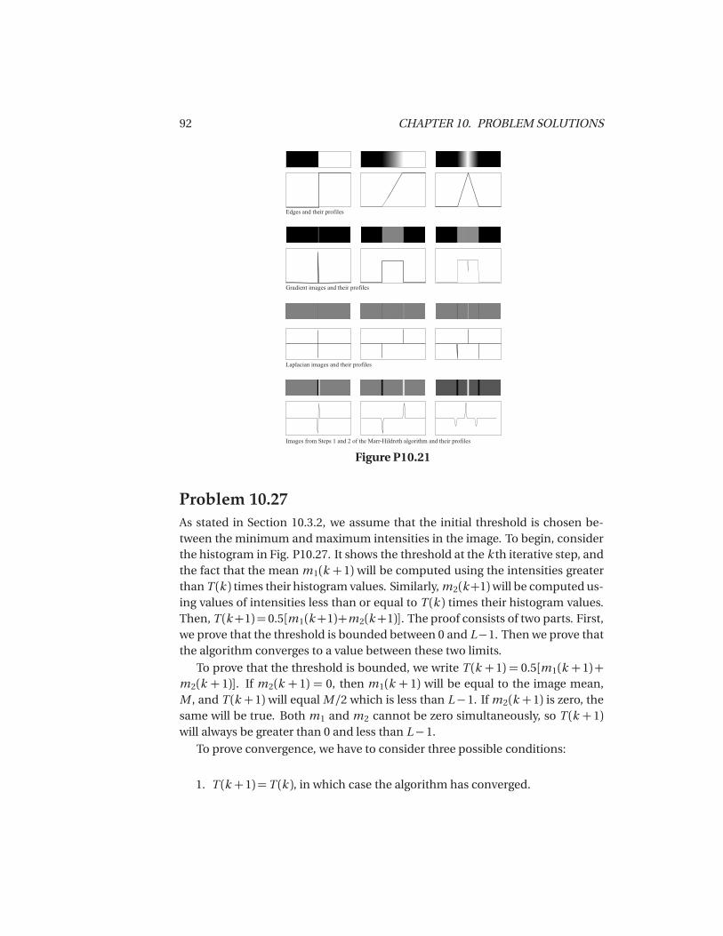
92 CHAPTER 10. PROBLEM SOLUTIONS
Edges and their profiles
Gradient images and their profiles
Laplacian images and their profiles
Images from Steps 1 and 2 of the Marr-Hildreth algorithm and their profiles
Figure P10.21
Problem 10.27As stated in Section 10.3.2, we assume that the initial threshold is chosen be-tween the minimum and maximum intensities in the image. To begin, considerthe histogram in Fig. P10.27. It shows the threshold at the k th iterative step, andthe fact that the mean m1(k + 1) will be computed using the intensities greaterthan T (k ) times their histogram values. Similarly, m2(k+1)will be computed us-ing values of intensities less than or equal to T (k ) times their histogram values.Then, T (k+1) = 0.5[m1(k+1)+m2(k+1)]. The proof consists of two parts. First,we prove that the threshold is bounded between 0 and L−1. Then we prove thatthe algorithm converges to a value between these two limits.
To prove that the threshold is bounded, we write T (k + 1) = 0.5[m1(k + 1) +m2(k + 1)]. If m2(k + 1) = 0, then m1(k + 1) will be equal to the image mean,M , and T (k + 1) will equal M/2 which is less than L− 1. If m2(k + 1) is zero, thesame will be true. Both m1 and m2 cannot be zero simultaneously, so T (k + 1)will always be greater than 0 and less than L− 1.
To prove convergence, we have to consider three possible conditions:
1. T (k + 1) = T (k ), in which case the algorithm has converged.
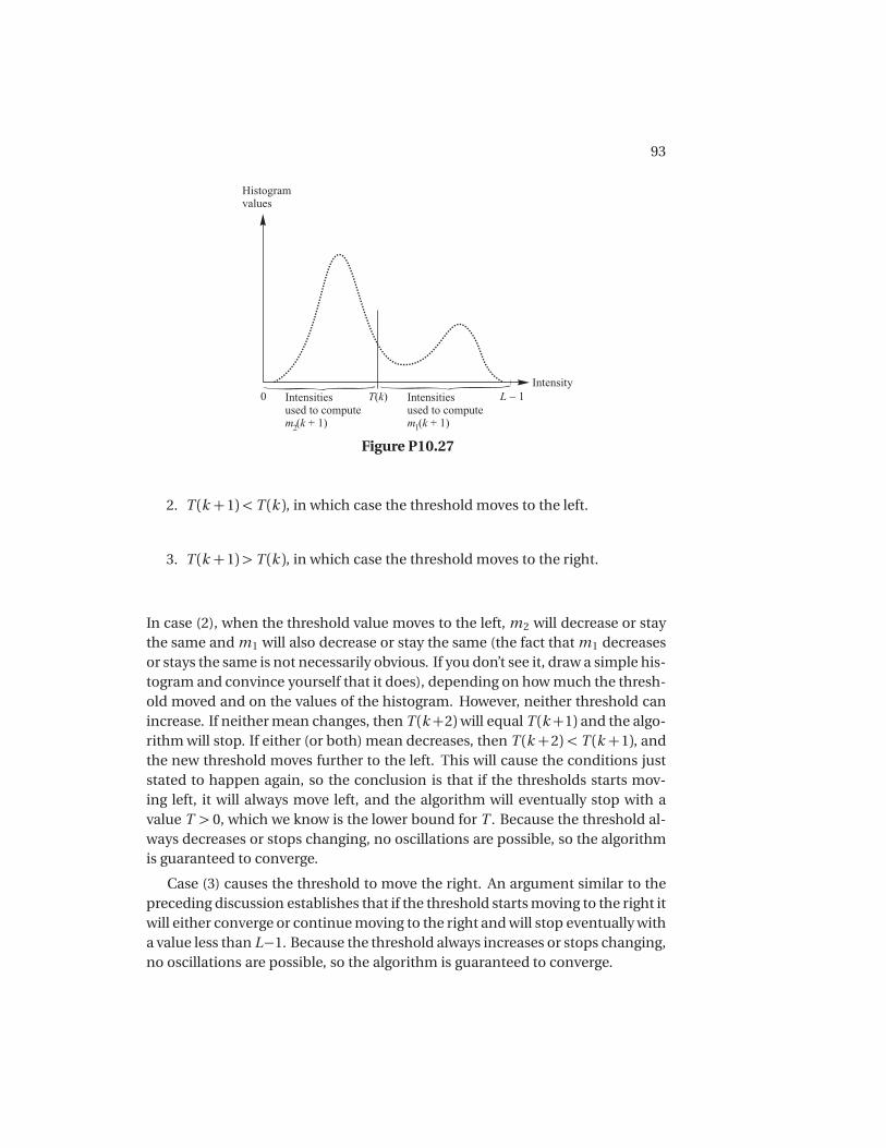
93
T k( )Intensitiesused to compute
( + 1)m k2
Intensitiesused to compute
( + 1)m k1
Intensity
Histogramvalues
}}L 1�0
Figure P10.27
2. T (k + 1)< T (k ), in which case the threshold moves to the left.
3. T (k + 1)> T (k ), in which case the threshold moves to the right.
In case (2), when the threshold value moves to the left, m2 will decrease or staythe same and m1 will also decrease or stay the same (the fact that m1 decreasesor stays the same is not necessarily obvious. If you don’t see it, draw a simple his-togram and convince yourself that it does), depending on how much the thresh-old moved and on the values of the histogram. However, neither threshold canincrease. If neither mean changes, then T (k+2)will equal T (k+1) and the algo-rithm will stop. If either (or both) mean decreases, then T (k +2)< T (k +1), andthe new threshold moves further to the left. This will cause the conditions juststated to happen again, so the conclusion is that if the thresholds starts mov-ing left, it will always move left, and the algorithm will eventually stop with avalue T > 0, which we know is the lower bound for T . Because the threshold al-ways decreases or stops changing, no oscillations are possible, so the algorithmis guaranteed to converge.
Case (3) causes the threshold to move the right. An argument similar to thepreceding discussion establishes that if the threshold starts moving to the right itwill either converge or continue moving to the right and will stop eventually witha value less than L−1. Because the threshold always increases or stops changing,no oscillations are possible, so the algorithm is guaranteed to converge.

94 CHAPTER 10. PROBLEM SOLUTIONS
Intensity
Histogramvalues
L 1�0 L/2
Intensitiesof background
Intensitiesof objects
Imin } }M
Figure P10.29
Problem 10.29The value of the the threshold at convergence is independent of the initial valueif the initial value of the threshold is chosen between the minimum and max-imum intensity of the image (we know from Problem 10.27 that the algorithmconverges under this condition). The final threshold is not independent of theinitial value chosen for T if that value does not satisfy this condition. For ex-ample, consider an image with the histogram in Fig. P10.29. Suppose that weselect the initial threshold T (1) = 0. Then, at the next iterative step, m2(2) = 0,m1(2) = M , and T (2) = M/2. Because m2(2) = 0, it follows that m2(3) = 0,m1(3) =M , and T (3) = T (2) =M/2. Any following iterations will yield the sameresult, so the algorithm converges with the wrong value of threshold. If we hadstarted with Imin < T (1)< Imax, the algorithm would have converged properly.
Problem 10.30(a) For a uniform histogram, we can view the intensity levels as points of unitmass along the intensity axis of the histogram. Any values m1(k ) and m2(k )are the means of the two groups of intensity values G1 and G2. Because the his-togram is uniform, these are the centers of mass of G1 and G2. We know from thesolution of Problem 10.27 that if T starts moving to the right, it will always movein that direction, or stop. The same holds true for movement to the left. Now,assume that T (k ) has arrived at the center of mass (average intensity). Becauseall points have equal "weight" (remember the histogram is uniform), if T (k + 1)moves to the right G2 will pick up, say, Q new points. But G1 will lose the samenumber of points, so the sum m1 +m2 will be the same and the algorithm willstop.

95
Problem 10.32(a)
σ2B = P1(m 1−mG )2+P2(m 2−mG )2
= P1(m1− (P1m1+P2m2)]2+P2[m2− (P1m1+P2m2)]2
= P1[m 1−m1(1−P 2)−P2m2]2+P2[m2−P1m1−m2(1−P1)]2
= P1[P2m1−P2m2]2+P2[P1m2−P1m1]2
= P1P22 (m1−m2)2+P2P2
1 (m1−m2)2
= (m1−m2)2[P1P22 +P2P2
1 ]
= (m1−m2)2[P1P2(P2+P1)]
= P1P2(m1−m2)2
we used the facts that mG = P1m1+P2m2 and P1+P2 = 1. This proves the firstpart of Eq. (10.3-15).
(b) First, we have to show that
m2(k ) =mG −m (k )
1−P1(k ).
This we do as follows:
m2(k ) =1
P2(k )
L−1∑i=k+1
i pi
=1
1−P1(k )
L−1∑i=k+1
i pi
=1
1−P1(k )
⎡⎣L−1∑
i=0
i pi −k∑
i=0
i pi
⎤⎦
=mG −m (k )
1−P1(k ).
Then,
σ2B = P1P2(m1−m2)2
= P1P2
�m
P1− mG −m
1−P1
�2
= P1(1−P1)�
m −P1mG
P1(1−P1)
�2
=(mG P1−m )2
P1(1−P1).
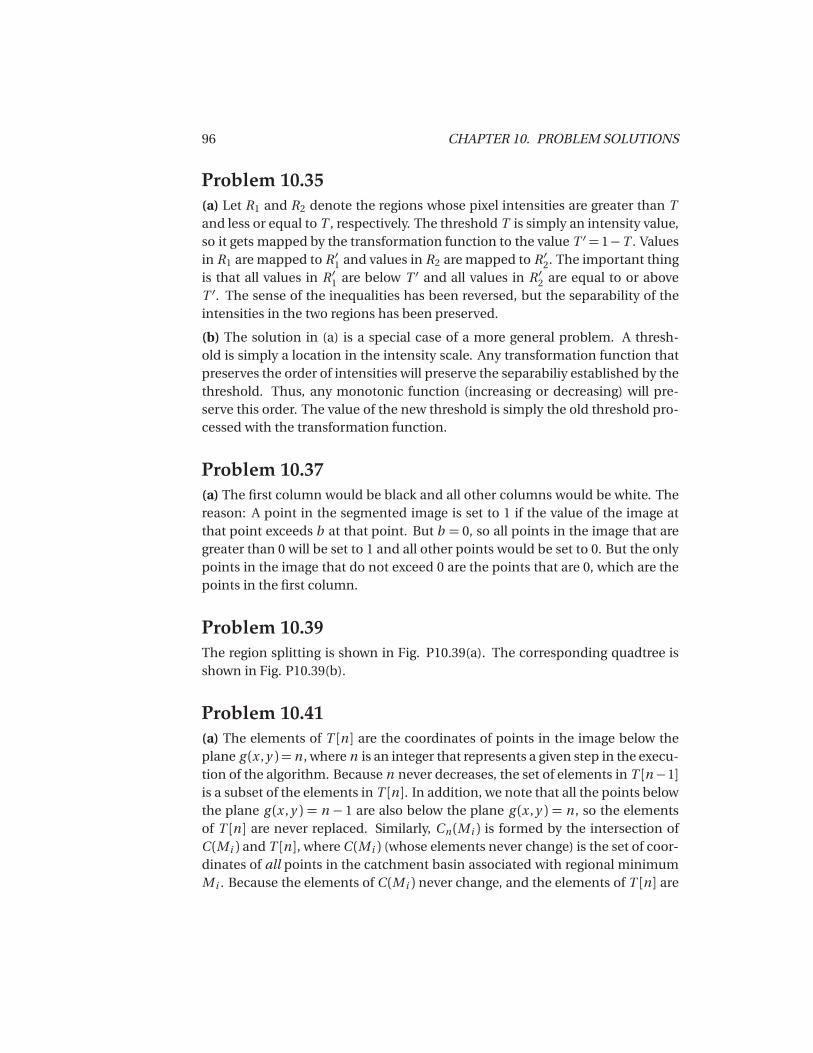
96 CHAPTER 10. PROBLEM SOLUTIONS
Problem 10.35(a) Let R1 and R2 denote the regions whose pixel intensities are greater than Tand less or equal to T , respectively. The threshold T is simply an intensity value,so it gets mapped by the transformation function to the value T ′ = 1−T . Valuesin R1 are mapped to R ′1 and values in R2 are mapped to R ′2. The important thingis that all values in R ′1 are below T ′ and all values in R ′2 are equal to or aboveT ′. The sense of the inequalities has been reversed, but the separability of theintensities in the two regions has been preserved.
(b) The solution in (a) is a special case of a more general problem. A thresh-old is simply a location in the intensity scale. Any transformation function thatpreserves the order of intensities will preserve the separabiliy established by thethreshold. Thus, any monotonic function (increasing or decreasing) will pre-serve this order. The value of the new threshold is simply the old threshold pro-cessed with the transformation function.
Problem 10.37(a) The first column would be black and all other columns would be white. Thereason: A point in the segmented image is set to 1 if the value of the image atthat point exceeds b at that point. But b = 0, so all points in the image that aregreater than 0 will be set to 1 and all other points would be set to 0. But the onlypoints in the image that do not exceed 0 are the points that are 0, which are thepoints in the first column.
Problem 10.39The region splitting is shown in Fig. P10.39(a). The corresponding quadtree isshown in Fig. P10.39(b).
Problem 10.41(a) The elements of T [n ] are the coordinates of points in the image below theplane g (x ,y ) = n , where n is an integer that represents a given step in the execu-tion of the algorithm. Because n never decreases, the set of elements in T [n−1]is a subset of the elements in T [n ]. In addition, we note that all the points belowthe plane g (x ,y ) = n − 1 are also below the plane g (x ,y ) = n , so the elementsof T [n ] are never replaced. Similarly, Cn (Mi ) is formed by the intersection ofC (Mi ) and T [n ], where C (Mi ) (whose elements never change) is the set of coor-dinates of all points in the catchment basin associated with regional minimumMi . Because the elements of C (Mi ) never change, and the elements of T [n ] are
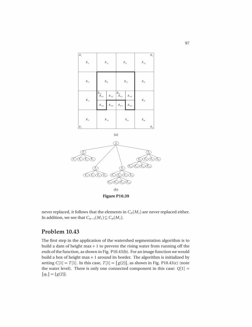
97
1
11 12 13 14
2
21 22 23 24
3
31 32 33 34
321 322 323 324
4
41 42 43 44
411 412 413 414
1
11 12
13 14
2
21 22
23 24
3
31
32
33 34
4
41
42
43 44
321 322
323 324
411 412
413 414
Figure P10.39
never replaced, it follows that the elements in Cn (Mi ) are never replaced either.In addition, we see that Cn−1(Mi )⊆Cn (Mi ).
Problem 10.43The first step in the application of the watershed segmentation algorithm is tobuild a dam of height max+ 1 to prevent the rising water from running off theends of the function, as shown in Fig. P10.43(b). For an image function we wouldbuild a box of height max+ 1 around its border. The algorithm is initialized bysetting C [1] = T [1]. In this case, T [1] =
g (2)
�, as shown in Fig. P10.43(c) (note
the water level). There is only one connected component in this case: Q[1] =q1�= {g (2)}.
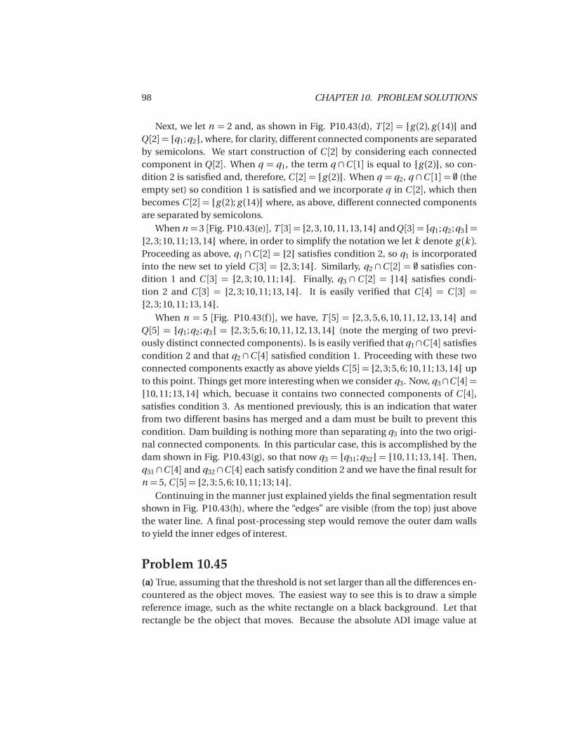
98 CHAPTER 10. PROBLEM SOLUTIONS
Next, we let n = 2 and, as shown in Fig. P10.43(d), T [2] = {g (2), g (14)} andQ[2] = {q1;q2}, where, for clarity, different connected components are separatedby semicolons. We start construction of C [2] by considering each connectedcomponent in Q[2]. When q = q1, the term q ∩C [1] is equal to {g (2)}, so con-dition 2 is satisfied and, therefore, C [2] = {g (2)}. When q = q2, q ∩C [1] = � (theempty set) so condition 1 is satisfied and we incorporate q in C [2], which thenbecomes C [2] = {g (2); g (14)} where, as above, different connected componentsare separated by semicolons.
When n = 3 [Fig. P10.43(e)], T [3] = {2,3,10,11,13,14} andQ[3] = {q1;q2;q3}={2,3;10,11;13,14} where, in order to simplify the notation we let k denote g (k ).Proceeding as above, q1 ∩C [2] = {2} satisfies condition 2, so q1 is incorporatedinto the new set to yield C [3] = {2,3;14}. Similarly, q2 ∩C [2] = � satisfies con-dition 1 and C [3] = {2,3;10,11;14}. Finally, q3 ∩ C [2] = {14} satisfies condi-tion 2 and C [3] = {2,3;10,11;13,14}. It is easily verified that C [4] = C [3] ={2,3;10,11;13,14}.
When n = 5 [Fig. P10.43(f)], we have, T [5] = {2,3,5,6,10,11,12,13, 14} andQ[5] = {q1;q2;q3} = {2,3;5,6;10,11,12,13, 14} (note the merging of two previ-ously distinct connected components). Is is easily verified that q1∩C [4] satisfiescondition 2 and that q2 ∩C [4] satisfied condition 1. Proceeding with these twoconnected components exactly as above yields C [5] = {2,3;5,6;10,11;13,14} upto this point. Things get more interesting when we consider q3. Now, q3∩C [4] ={10,11;13,14} which, becuase it contains two connected components of C [4],satisfies condition 3. As mentioned previously, this is an indication that waterfrom two different basins has merged and a dam must be built to prevent thiscondition. Dam building is nothing more than separating q3 into the two origi-nal connected components. In this particular case, this is accomplished by thedam shown in Fig. P10.43(g), so that now q3 = {q31;q32}= {10,11;13,14}. Then,q31 ∩C [4] and q32 ∩C [4] each satisfy condition 2 and we have the final result forn = 5, C [5] = {2,3;5,6;10,11;13;14}.
Continuing in the manner just explained yields the final segmentation resultshown in Fig. P10.43(h), where the “edges” are visible (from the top) just abovethe water line. A final post-processing step would remove the outer dam wallsto yield the inner edges of interest.
Problem 10.45(a) True, assuming that the threshold is not set larger than all the differences en-countered as the object moves. The easiest way to see this is to draw a simplereference image, such as the white rectangle on a black background. Let thatrectangle be the object that moves. Because the absolute ADI image value at
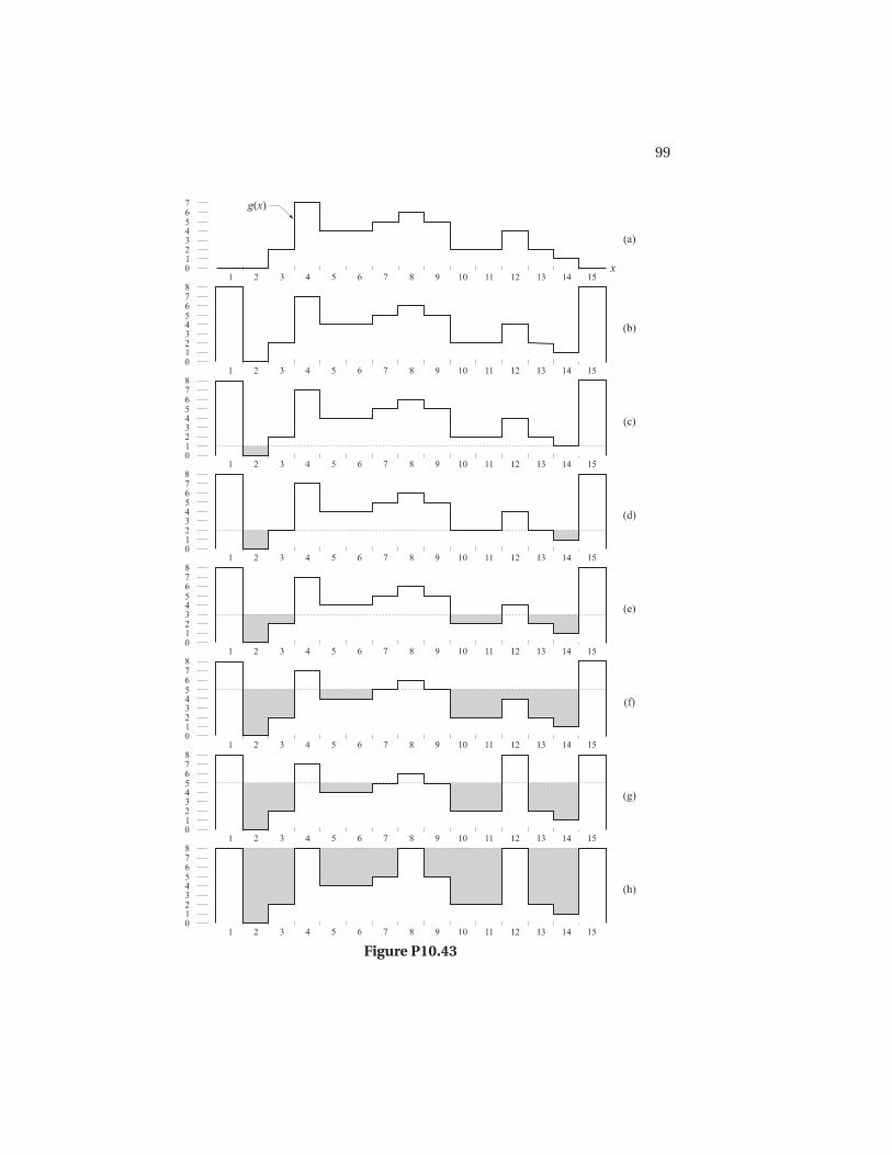
99
Figure P10.43

100 CHAPTER 10. PROBLEM SOLUTIONS
any location is the absolute difference between the reference and the new im-age, it is easy to see that as the object enters areas that are background in thereference image, the absolute difference will change from zero to nonzero at thenew area occupied by the moving object. Thus, as long as the object moves, thedimension of the absolute ADI will grow.
Problem 10.47Recall that velocity is a vector, whose magnitude is speed. Function g x is aone-dimensional "record" of the position of the moving object as a function oftime (frame rate). The value of velocity (speed) is determined by taking the firstderivative of this function. To determine whether velocity is positive or negativeat a specific time, n , we compute the instantaneous acceleration (rate of changeof speed) at that point; that is we compute the second derivate of g x . Viewedanother way, we determine direction by computing the derivative of the deriva-tive of g x . But, the derivative at a point is simply the tangent at that point. Ifthe tangent has a positive slope, the velocity is positive; otherwise it is negativeor zero. Because g x is a complex quantity, its tangent is given by the ratio of itsimaginary to its real part. This ratio is positive when S1x and S2x have the samesign, which is what we started out to prove.
Problem 10.49(a) It is given that 10% of the image area in the horizontal direction is occupiedby a bullet that is 2.5 cm long. Because the imaging device is square (256× 256elements) the camera looks at an area that is 25 cm× 25 cm, assuming no opticaldistortions. Thus, the distance between pixels is 25/256=0.098 cm/pixel. Themaximum speed of the bullet is 1000 m/sec= 100,000 cm/sec. At this speed, thebullet will travel 100,000/0.98= 1.02×106 pixels/sec. It is required that the bulletnot travel more than one pixel during exposure. That is, (1.02×106 pixels/sec)×K sec ≤ 1 pixel. So, K ≤ 9.8× 10⁻⁷ sec.

NOTICE This manual is intended for your personal use only. Copying, printing, posting, or any form of printed or electronic distribution of any part of this manual constitutes a violation of copyright law. As a security measure, this manual was encrypted during download with the serial number of your book, and with your personal information. Any printed or electronic copies of this file will bear that encryption, which will tie the copy to you. Please help us defeat piracy of intellectual property, one of the principal reasons for the increase in the cost of books. -------------------------------

Chapter 11
Problem Solutions
Problem 11.1(a) The key to this problem is to recognize that the value of every element in achain code is relative to the value of its predecessor. The code for a boundarythat is traced in a consistent manner (e.g., clockwise) is a unique circular set ofnumbers. Starting at different locations in this set does not change the struc-ture of the circular sequence. Selecting the smallest integer as the starting pointsimply identifies the same point in the sequence. Even if the starting point isnot unique, this method would still give a unique sequence. For example, thesequence 101010 has three possible starting points, but they all yield the samesmallest integer 010101.
Problem 11.3(a) The rubber-band approach forces the polygon to have vertices at every in-flection of the cell wall. That is, the locations of the vertices are fixed by thestructure of the inner and outer walls. Because the vertices are joined by straightlines, this produces the minimum-perimeter polygon for any given wall config-uration.
Problem 11.4(a) When the B vertices are mirrored, they coincide with the two white verticesin the corners, so they become collinear with the corner vertices. The algorithmignores collinear vertices, so the small indentation will not be detected.
(b) When the indentation is deeper than one pixel (but still 1 pixel wide) we havethe situation shown in Fig. P11.4. Note that the B vertices cross after mirroring.
101
102 CHAPTER 11. PROBLEM SOLUTIONS
Order and location of vertices
before mirroring the verticesB
Order and location of vertices
after mirroring the verticesB
1 2
34
1
2
3
4
Figure P11.4
Referring to the bottom figure, when the algorithm gets to vertex 2, vertex 1 willbe identified as a vertex of the MPP, so the algorithm is initialized at that step.Because of initialization, vertex 2 is visited again. It will be collinear with W C
and VL, so BC will be set at the location of vertex 2. When vertex 3 is visited,sgn(VL,W C,V3) will be 0, so BC will be set at vertex 3. When vertex 4 is visited,sgn(1,3,4)will be negative, so VL will be set to vertex 3 and the algorithm is reini-tialized. Because vertex 2 will never be visited again, it will never become a ver-tex of the MPP. The next MPP vertex to be detected will be vertex 4. Therefore,indentations 2 pixels or greater in depth and 1 pixel wide will be represented bythe sequence 1−3−4 in the second figure. Thus, the algorithm solves the cross-ing caused by the mirroring of the two B vertices by keeping only one vertex.This is a general result for 1-pixel wide, 2 pixel (or greater) deep intrusions.
Problem 11.5
(a) The resulting polygon would contain all the boundary pixels.
Problem 11.6
(a) The solution is shown in Fig. P11.6(b).

103
Figure P11.6
Problem 11.7(a) From Fig. P11.7(a), we see that the distance from the origin to the triangle isgiven by
r (θ ) =D0
cosθ0◦ ≤ θ < 60◦
=D0
cos(120◦ −θ ) 60◦ ≤ θ < 120◦
=D0
cos(180◦ −θ ) 120◦ ≤ θ < 180◦
=D0
cos(240◦ −θ ) 180◦ ≤ θ < 240◦
=D0
cos(300◦ −θ ) 240◦ ≤ θ < 300◦
=D0
cos(360◦ −θ ) 300◦ ≤ θ < 360◦
Figure P11.7

104 CHAPTER 11. PROBLEM SOLUTIONS
Figure P11.8
Figure P11.10
where D0 is the perpendicular distance from the origin to one of the sides of thetriangle, and D = D0/cos(60◦) = 2D0. Once the coordinates of the vertices ofthe triangle are given, determining the equation of each straight line is a simpleproblem, and D0 (which is the same for the three straight lines) follows fromelementary geometry.
Problem 11.8The solutions are shown in Fig. P11.8.
Problem 11.9(a) In the first case, N (p ) = 5, S(p ) = 1, p2 ·p4 ·p6 = 0, and p4 ·p6 ·p8 = 0, so Eq.(11.1-4) is satisfied and p is flagged for deletion. In the second case, N (p ) = 1, soEq. (11.1-4) is violated and p is left unchanged. In the third case p2 ·p4 ·p6 = 1and p4 ·p6 · p8 = 1, so conditions (c) and (d) of Eq. (11.1-4) are violated and pis left unchanged. In the forth case S(p ) = 2, so condition (b) is violated and p isleft unchanged.
Problem 11.10(a) The result is shown in Fig. P11.10(b).

105
Problem 11.11
(a) The number of symbols in the first difference is equal to the number of seg-ment primitives in the boundary, so the shape order is 12.
Problem 11.14
The mean is sufficient.
Problem 11.16
This problem can be solved by using two descriptors: holes and the convex de-ficiency (see Section 9.5.4 regarding the convex hull and convex deficiency of aset). The decision making process can be summarized in the form of a simpledecision, as follows: If the character has two holes, it is an 8. If it has one holeit is a 0 or a 9. Otherwise, it is a 1 or an X. To differentiate between 0 and 9 wecompute the convex deficiency. The presence of a ”significant” deficiency (say,having an area greater than 20% of the area of a rectangle that encloses the char-acter) signifies a 9; otherwise we classify the character as a 0. We follow a similarprocedure to separate a 1 from an X. The presence of a convex deficiency withfour components whose centroids are located approximately in the North, East,West, and East quadrants of the character indicates that the character is an X.Otherwise we say that the character is a 1. This is the basic approach. Imple-mentation of this technique in a real character recognition environment has totake into account other factors such as multiple ”small” components in the con-vex deficiency due to noise, differences in orientation, open loops, and the like.However, the material in Chapters 3, 9 and 11 provide a solid base from whichto formulate solutions.
Problem 11.17
(b) Normalize the matrix by dividing each component by 19600 + 200 + 20000= 39800:
0.4925 0.00500 0.5025
so p11 = 0.4925, p12 = 0.005, p21 = 0, and p22 = 0.5025.
106 CHAPTER 11. PROBLEM SOLUTIONS
Problem 11.19(a) The image is
0 1 0 1 01 0 1 0 10 1 0 1 01 0 1 0 10 1 0 1 0
.
Let z 1 = 0 and z 2 = 1. Because there are only two intensity levels, matrix G is oforder 2×2. Element g 11 is the number of pixels valued 0 located one pixel to theright of a 0. By inspection, g 11 = 0. Similarly, g 12 = 10, g 21 = 10, and g 22 = 0.The total number of pixels satisfying the predicate P is 20, so the normalizedco-occurrence matrix is
G=
'0 1/2
1/2 0
(.
Problem 11.21The mean square error, given by Eq. (11.4-12), is the sum of the eigenvalueswhose corresponding eigenvectors are not used in the transformation. In thisparticular case, the four smallest eigenvalues are applicable (see Table 11.6), sothe mean square error is
em s =6∑
j=3
λj = 1729.
The maximum error occurs when K = 0 in Eq. (11.4-12) which then is the sumof all the eigenvalues, or 15039 in this case. Thus, the error incurred by usingonly the two eigenvectors corresponding to the largest eigenvalues is just 11.5 %of the total possible error.
Problem 11.23When the boundary is symmetric about the both the major and minor axes andboth axes intersect at the centroid of the boundary.
Problem 11.25We can compute a measure of texture using the expression
R(x ,y ) = 1− 1
1+σ2(x ,y )

107
where σ2(x ,y ) is the intensity variance computed in a neighborhood of (x ,y ).The size of the neighborhood must be sufficiently large so as to contain enoughsamples to have a stable estimate of the mean and variance. Neighborhoods ofsize 7× 7 or 9× 9 generally are appropriate for a low-noise case such as this.
Because the variance of normal wafers is known to be 400, we can obtain anormal value for R(x ,y ) by using σ2 = 400 in the above equation. An abnor-mal region will have a variance of about (50)2 = 2,500 or higher, yielding a largervalue of R(x ,y ). The procedure then is to compute R(x ,y ) at every point (x ,y )and label that point as 0 if it is normal and 1 if it is not. At the end of this pro-cedure we look for clusters of 1’s using, for example, connected components(see Section 9.5.3 regarding computation of connected components) . If thearea (number of pixels) of any connected component exceeds 400 pixels, thenwe classify the sample as defective.

NOTICE This manual is intended for your personal use only. Copying, printing, posting, or any form of printed or electronic distribution of any part of this manual constitutes a violation of copyright law. As a security measure, this manual was encrypted during download with the serial number of your book, and with your personal information. Any printed or electronic copies of this file will bear that encryption, which will tie the copy to you. Please help us defeat piracy of intellectual property, one of the principal reasons for the increase in the cost of books. -------------------------------

Chapter 12
Problem Solutions
Problem 12.2From the definition of the Euclidean distance,
Dj (x) =//x−mj
//= �(x−mj )T (x−mj )
.1/2
Because Dj (x) is non-negative, choosing the smallest Dj (x) is the same as choos-ing the smallest D2
j (x), where
D2j (x) =
//x−mj
//2= (x−mj )T (x−mj )
= xT x− 2xT mj +mTj mj
= xT x−2
�xT mj − 1
2mT
j mj
�.
We note that the term xT x is independent of j (that is, it is a constant with re-spect to j in D2
j (x), j = 1,2, . . .). Thus, choosing the minimum of D2j (x) is equiva-
lent to choosing the maximum of�
xT mj − 12 mT
j mj
�.
Problem 12.4The solution is shown in Fig. P12.4, where the x ’s are treated as voltages andthe Y ’s denote impedances. From basic circuit theory, the currents, I ’s, are theproducts of the voltages times the impedances. The system operates by select-ing the maximum current, which corresponds to the best match and, therefore,
109
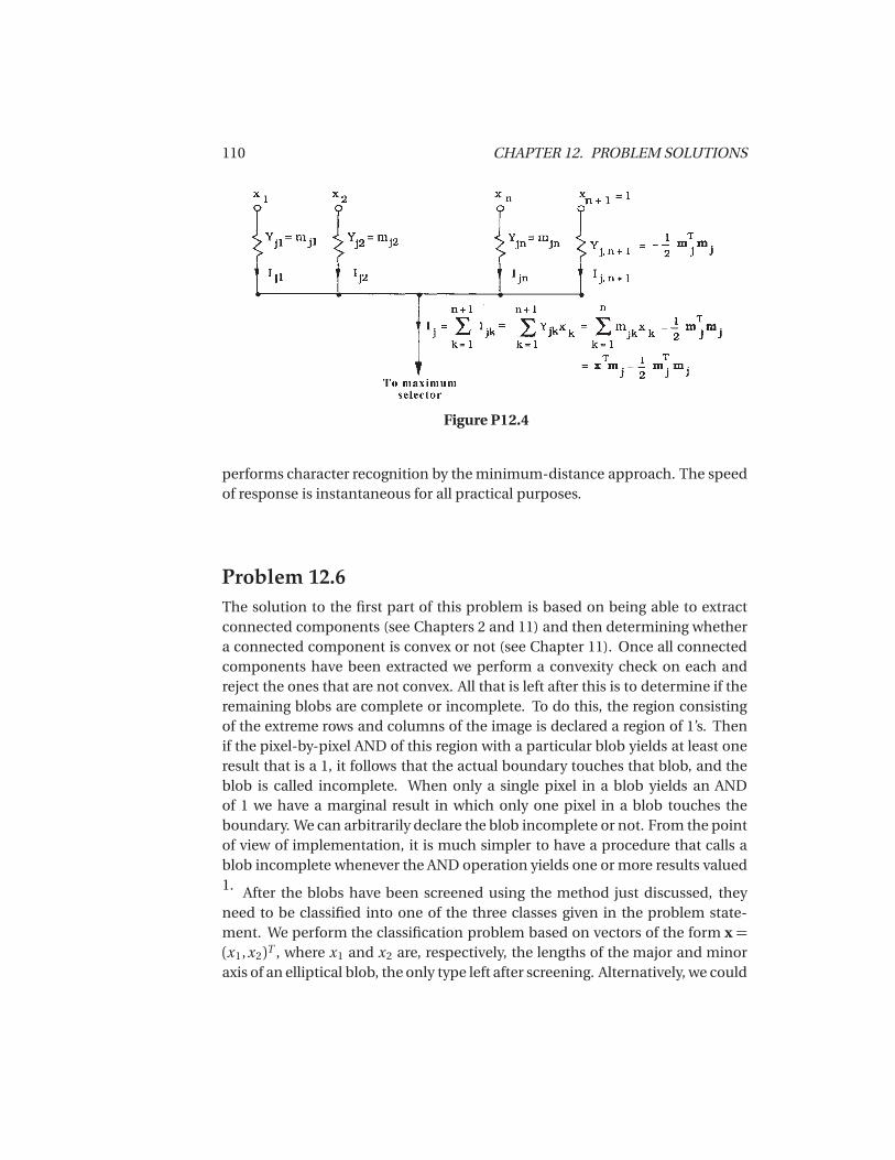
110 CHAPTER 12. PROBLEM SOLUTIONS
Figure P12.4
performs character recognition by the minimum-distance approach. The speedof response is instantaneous for all practical purposes.
Problem 12.6The solution to the first part of this problem is based on being able to extractconnected components (see Chapters 2 and 11) and then determining whethera connected component is convex or not (see Chapter 11). Once all connectedcomponents have been extracted we perform a convexity check on each andreject the ones that are not convex. All that is left after this is to determine if theremaining blobs are complete or incomplete. To do this, the region consistingof the extreme rows and columns of the image is declared a region of 1’s. Thenif the pixel-by-pixel AND of this region with a particular blob yields at least oneresult that is a 1, it follows that the actual boundary touches that blob, and theblob is called incomplete. When only a single pixel in a blob yields an ANDof 1 we have a marginal result in which only one pixel in a blob touches theboundary. We can arbitrarily declare the blob incomplete or not. From the pointof view of implementation, it is much simpler to have a procedure that calls ablob incomplete whenever the AND operation yields one or more results valued1. After the blobs have been screened using the method just discussed, theyneed to be classified into one of the three classes given in the problem state-ment. We perform the classification problem based on vectors of the form x =(x1,x2)T , where x1 and x2 are, respectively, the lengths of the major and minoraxis of an elliptical blob, the only type left after screening. Alternatively, we could
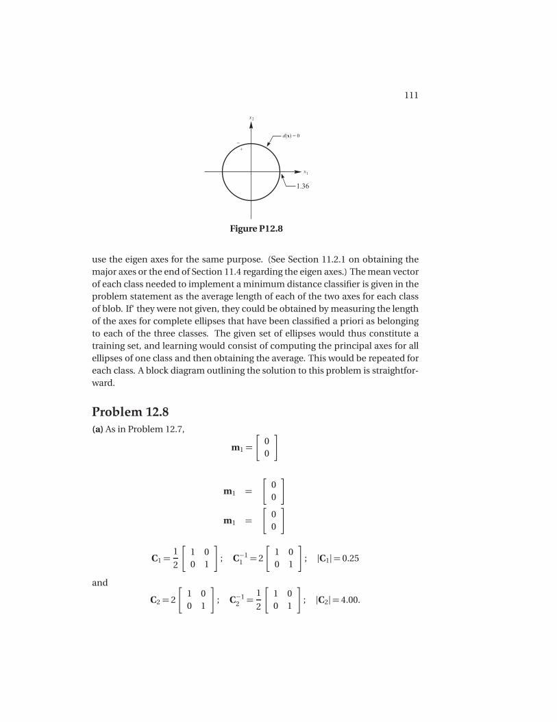
111
x1
x2
+
�
d( ) = 0x
1.36
Figure P12.8
use the eigen axes for the same purpose. (See Section 11.2.1 on obtaining themajor axes or the end of Section 11.4 regarding the eigen axes.) The mean vectorof each class needed to implement a minimum distance classifier is given in theproblem statement as the average length of each of the two axes for each classof blob. If‘ they were not given, they could be obtained by measuring the lengthof the axes for complete ellipses that have been classified a priori as belongingto each of the three classes. The given set of ellipses would thus constitute atraining set, and learning would consist of computing the principal axes for allellipses of one class and then obtaining the average. This would be repeated foreach class. A block diagram outlining the solution to this problem is straightfor-ward.
Problem 12.8(a) As in Problem 12.7,
m1 =
'00
(
m1 =
'00
(
m1 =
'00
(
C1 =1
2
'1 00 1
(; C−1
1 = 2
'1 00 1
(; |C1|= 0.25
and
C2 = 2
'1 00 1
(; C−1
2 =1
2
'1 00 1
(; |C2|= 4.00.
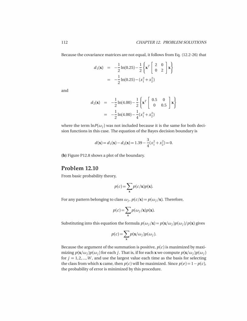
112 CHAPTER 12. PROBLEM SOLUTIONS
Because the covariance matrices are not equal, it follows from Eq. (12.2-26) that
d 1(x) = −1
2ln(0.25)− 1
2
)xT
'2 00 2
(x
0
= −1
2ln(0.25)− (x 2
1 +x 22 )
and
d 2(x) = −1
2ln(4.00)− 1
2
)xT
'0.5 00 0.5
(x
0
= −1
2ln(4.00)− 1
4(x 2
1 +x 22 )
where the term lnP(ωj ) was not included because it is the same for both deci-sion functions in this case. The equation of the Bayes decision boundary is
d (x) = d 1(x)−d 2(x) = 1.39− 3
4(x 2
1 +x 22) = 0.
(b) Figure P12.8 shows a plot of the boundary.
Problem 12.10From basic probability theory,
p (c ) =∑
x
p (c/x)p (x).
For any pattern belonging to classωj , p (c/x) = p (ωj /x). Therefore,
p (c ) =∑
x
p (ωj /x)p (x).
Substituting into this equation the formula p (ωj /x) = p (x/ωj )p (ωj )/p (x) gives
p (c ) =∑
x
p (x/ωj )p (ωj ).
Because the argument of the summation is positive, p (c ) is maximized by maxi-mizing p (x/ωj )p (ωj ) for each j . That is, if for each x we compute p (x/ωj )p (ωj )for j = 1,2, ...,W , and use the largest value each time as the basis for selectingthe class from which x came, then p (c ) will be maximized. Since p (e ) = 1−p (c ),the probability of error is minimized by this procedure.
113
Problem 12.12We start by taking the partial derivative of J with respect to w:
∂ J
∂ w=
1
2
�ysgn(wT y)− y
where, by definition, sgn(wT y) = 1 if wT y > 0, and sgn(wT y) = −1 otherwise.Substituting the partial derivative into the general expression given in the prob-lem statement gives
w(k + 1) =w(k )+c
2
-y(k)− y(k)sgn
�w(k)T y(k)
.where y(k ) is the training pattern being considered at the k th iterative step. Sub-stituting the definition of the sgn function into this result yields
w(k + 1) =w(k )+ c
)0 if w(k)T y(k)y(k ) otherwise
where c > 0 and w(1) is arbitrary. This expression agrees with the formulationgiven in the problem statement.
Problem 12.14The single decision function that implements a minimum distance classifier fortwo classes is of the form
d i j (x) = xT (mi −mj )− 1
2(mT
i mi −mTj mj ).
Thus, for a particular pattern vector x, when d i j (x)> 0, x is assigned to classω1
and, when d i j (x) < 0, x is assigned to class ω2. Values of x for which d i j (x) = 0are on the boundary (hyperplane) separating the two classes. By letting w =(mi −mj ) and wn+1 = − 1
2 (mTi mi −mT
j mj ), we can express the above decisionfunction in the form
d (x) =wT x−wn+1.
This is recognized as a linear decision function in n dimensions, which is imple-mented by a single layer neural network with coefficients
wk = (mi k −m j k ) k = 1,2, . . . ,n
and
θ =wn+1 =−1
2(mT
i mi −mTj mj ).

114 CHAPTER 12. PROBLEM SOLUTIONS
Problem 12.16(a) When P(ωi ) = P(ωj ) and C= I.
(b) No. The minimum distance classifier implements a decision function that isthe perpendicular bisector of the line joining the two means. If the probabilitydensities are known, the Bayes classifier is guaranteed to implement an opti-mum decision function in the minimum average loss sense. The generalizeddelta rule for training a neural network says nothing about these two criteria, soit cannot be expected to yield the decision functions in Problems 12.14 or 12.15.
Problem 12.18All that is needed is to generate for each class training vectors of the form x =(x1,x2)T , where x1 is the length of the major axis and x2 is the length of the mi-nor axis of the blobs comprising the training set. These vectors would then beused to train a neural network using, for example, the generalized delta rule.(Because the patterns are in 2D, it is useful to point out to students that the neu-ral network could be designed by inspection in the sense that the classes couldbe plotted, the decision boundary of minimum complexity obtained, and thenits coefficients used to specify the neural network. In this case the classes are farapart with respect to their spread, so most likely a single layer network imple-menting a linear decision function could do the job.)
Problem 12.20The first part of Eq. (12.3-3) is proved by noting that the degree of similarity, k , isnon-negative, so D(A, B ) = 1/k ≥ 0. Similarly, the second part follows from thefact that k is infinite when (and only when) the shapes are identical.
To prove the third part we use the definition of D to write
D(A,C )≤max [D(A, B ),D(B ,C )]
as1
ka c≤max
�1
kab,
1
kbc
�
or, equivalently,ka c ≥min [kab ,kbc ]
where ki j is the degree of similarity between shape i and shape j . Recall fromthe definition that k is the largest order for which the shape numbers of shape iand shape j still coincide. As Fig. 12.24(b) illustrates, this is the point at whichthe figures ”separate” as we move further down the tree (note that k increases

115
Figure P12.20
as we move further down the tree). We prove that ka c ≥ min[kab ,kbc ] by con-tradiction. For ka c ≤min[kab ,kbc ] to hold, shape A has to separate from shapeC before (1) shape A separates from shape B , and (2) before shape B separatesfrom shape C , otherwise kab ≤ ka c or kbc ≤ ka c , which automatically vio-lates the condition ka c <min[kab ,kbc ]. But, if (1) has to hold, then Fig. P12.20shows the only way that A can separate from C before separating from B . This,however, violates (2), which means that the condition ka c <min[kab ,kbc ] is vi-olated (we can also see this in the figure by noting that ka c = kbc which, sincekbc < kab , violates the condition). We use a similar argument to show that if(2) holds then (1) is violated. Thus, we conclude that it is impossible for thecondition ka c <min[kab ,kbc ] to hold, thus proving that ka c ≥min[kab ,kbc ] or,equivalently, that D(A,C )≤max[D(A, B ),D(B ,C )].