
Structured Computer Organization - WordPress.com...Chapter 1 INTRODUCTION 1 1.1 Structured Computer...
514
Structured Computer Organization Fourth Edition Andrew S. Tanenbaum With contributions from James R. Goodman Structured Computer Organization is the fourth edition of this best-selling introduction to computer hardware and architecture. It has been heavily revised to reflect the latest changes in the rapidly changing computer industry. Professor Tanenbaum has maintained his popular method of presenting the computer as a hierarchy of levels, each with a well-defined function. The book is written in a style and level of detail that covers all the major areas, but is still accessible to a broad range of readers. After an introductory chapter and a chapter about system organization (processors, memories, and I/O devices), we come to the core of the book: chapters on the digital logic level, the microarchitecture level, the instruction set architecture level, the operating system level, and the assembly language level. Finally, there is a chapter on the increasingly important topic of parallel computer architectures. New to this edition: • The running examples throughout the book are now the Pentium II, Sun UltraSPARC II, and Java Virtual Machine, inlcuding Sun's hardware Java chip that implements JVM • The input/output devices discussed in the computer systems organization chapter have been updated to emphasize modern technology such as RAID disks, CD-recordables, DVD, and color printers • Modern computer buses, such as the PCI bus and USB bus have been added to the digital logic level. • The microarchitecture level has been completely rewritten and updated as follows: Book Resources Overview
Transcript of Structured Computer Organization - WordPress.com...Chapter 1 INTRODUCTION 1 1.1 Structured Computer...
Structured Computer Organization
Fourth Edition
Andrew S. Tanenbaum With contributions from James R. Goodman
Structured Computer Organization is the fourth edition of this best-selling introduction to computer hardware and architecture. It has been heavily revised to reflect the latest changes in the rapidly changing computer industry. Professor Tanenbaum has maintained his popular method of presenting the computer as a hierarchy of levels, each with a well-defined function. The book is written in a style and level of detail that covers all the major areas, but is still accessible to a broad range of readers.
After an introductory chapter and a chapter about system organization (processors, memories, and I/O devices), we come to the core of the book: chapters on the digital logic level, the microarchitecture level, the instruction set architecture level, the operating system level, and the assembly language level. Finally, there is a chapter on the increasingly important topic of parallel computer architectures. New to this edition:
• The running examples throughout the book are now the Pentium II, Sun UltraSPARC II, and Java Virtual Machine, inlcuding Sun's hardware Java chip that implements JVM
• The input/output devices discussed in the computer systems organization chapter have been updated to emphasize modern technology such as RAID disks, CD-recordables, DVD, and color printers
• Modern computer buses, such as the PCI bus and USB bus have been added to the digital logic level.
• The microarchitecture level has been completely rewritten and updated as follows:
Book ResourcesOverview

o The detailed microprogrammed machine example illustrating data path control is now based on a subset of the Java Virtual Machine
o Design cost and performance tradeoffs are illustrated with a series of detailed examples culminating with the Mic-4 example that uses a seven-stage pipeline to introduce how modern computers such as the Pentium II work
o A new section on improving performance focuses on the most recent techniques such as caching, branch prediction, out-of-order execution, and speculative execution
• The instruction architecture level covers machine language using the new running examples.
• The operating system level includes examples for the Pentium II (Windows NT) and the UltraSPARC II (UNIX).
• New material on dynamic linking has been added to the assembly language level .
• The parallel computer architecture chapter has been completely rewritten and expanded to include a detailed treatment of multiprocessors (UMA, NUMA, and COMA), and multicomputers (MPP and COW).
• All code examples have been rewritten in Java.
With nearly 300 end-of-chapter exercises. an up-to-date annotated bibliography, figure files available for downloading, a Mic-1 simulator for student use, and a new instructor's manual, this book is ideal for courses in computer architecture or assembly language programming.

The first three editions of this book were based on the idea that a computer can be regarded as a hierarchy of levels, each one performing some well-defined function. This fundamental concept is as valid today as it was when the first edition came out, so it has been retained as the basis for the fourth edition. As in the first three editions, the digital logic level, the microarchitecture level, the instruction set architecture level, the operating system machine level, and the assembly language level are all discussed in detail (although we have changed some of the names to reflect modern practice).
Although the basic structure has been maintained, this fourth edition contains many changes, both small and large, that bring it up to date in the rapidly changing computer industry. For example, all the code examples, which were in Pascal, have been rewritten in Java, reflecting the popularity of Java in the computer world. Also, the example machines used have been brought up to date. The current examples are the Intel Pentium II, the Sun UltraSPARC II, and the Sun picoJava II, an embedded low-cost hardware Java chip.
Multiprocessors and parallel computers have also come in widespread use since the third edition, so the material on parallel architectures has been completely redone and greatly expanded, now covering a wide range of topics, from multiprocessors to COWs.
The book has become longer over the years (although still not as long as some other popular books on the subject). Such an expansion is inevitable as a subject develops and there is more known about it. As a result, when the book is used for a course, it may not always be possible to finish the book in a single course (e.g., in a trimester system). A possible approach would be to do all of Chaps. 1, 2, and 3, the first part of Chap. 4 (up through and including Sec. 4.4), and Chap. 5 as a bare minimum. The remaining time could be filled with the rest of Chap. 4, and parts of Chaps. 6, 7, and 8, depending on the interest of the instructor.
A chapter-by-chapter rundown of the major changes since the third edition follows. Chapter 1 still contains an historical overview of computer architecture, pointing out how we got where we are now and what the milestones were along the way. The enlarged spectrum of computers that exist is now discussed, and our three major examples (Pentium II, UltraSPARC II, and picoJava II) are introduced.
In Chapter 2, the material on input/output devices has been updated, emphasizing the technology of modern devices, including RAID disks, CD-Recordables, DVD, and color printers, among many others.
Chapter 3 (digital logic level) has undergone some revision and now treats computer buses and modern I/O chips. The major change here is additional
Book ResourcesPreface
material on buses, especially the PCI bus and the USB bus. The three new examples are described here at the chip level.
Chapter 4 (now called the microarchitecture level) has been completely rewritten. The idea of using a detailed example of a microprogrammed machine to illustrate the ideas of data path control has been retained, but the example machine is now a subset of the Java Virtual Machine. The underlying microarchitecture has been correspondingly changed. Several iterations of the design are given, showing what trade-offs are possible in terms of cost and performance. The last example, the Mic-4, uses a seven-stage pipeline and provides an easy introduction to how important modern computers, such as the Pentium II, work. A new section on improving performance has been added, focusing on the most recent techniques such as caching, branch prediction, (superscalar) out-of-order execution, speculative execution, and predication. The new example machines are discussed at the microarchitecture level.
Chapter 5 (now called the instruction set architecture level) deals with what many people refer to as \*(OQmachine language.\*(CQ The Pentium II, UltraSPARC II and Java Virtual Machine are used as the primary examples here.
Chapter 6 (operating system machine level) has examples for the Pentium II (Windows NT) and UltraSPARC II (UNIX). The former is new and has many features that are worth looking at, but UNIX is still a reliable workhorse at many universities and companies and is well worth examining in detail as well due to its simple and elegant design.
Chapter 7 (assembly language level) has been brought up to date by using examples from the machines we have been studying. New material on dynamic linking has been added as well.
Chapter 8 (parallel computer architectures) has been completely rewritten from the third edition. It now covers both multiprocessors (UMA, NUMA, and COMA) in detail, as well as multicomputers (MPP and COW).
The bibliography has been extensively revised and brought up to date. Well over two-thirds the references refer to works published after the third edition was published. Binary numbers and floating-point numbers have not undergone much change recently, so the appendices are largely the same as in the previous edition.
Finally, some problems have been revised and many new problems have been added since the third edition. Accordingly, a new problem solutions manual is available from Prentice Hall. It is available .I only to faculty members, who can request a free copy from their Prentice Hall representative.
A Web site for this book is available. PostScript files for all the illustrations used in the book are available electronically. They can be fetched and printed, for example, for making overhead sheets. In addition, a simulator and other and software tools are there too. The URL for this site is .HS .ti 0.25i \fIhttp://www.cs.vu.nl/\(tiast/sco4/\fP .HS The simulator and software tools

were produced by Ray Ontko. The author wishes to express his gratitude to Ray for producing these extremely useful programs.
A number of people have read (parts of) the manuscript and provided useful suggestions or have been helpful in other ways. In particular, I would like to thank Henri Bal, Alan Charlesworth, Stan Eisenstat, Kourosh Gharachorloo, Marcus Goncalves, Karen Panetta Lentz, Timothy Mattson, Harlan McGhan, Miles Murdocca, Kevin Normoyle, Mike O'Connor, Mitsunori Ogihara, Ray Ontko, Aske Plaat, William Potvin II, Nagarajan Prabhakaran. James H. Pugsley, Ronald N. Schroeder, Ryan Shoemaker, Charles Silio, Jr., and Dale Skrien for their help, for which I am most grateful. My students, especially Adriaan Bon, Laura de Vries, Dolf Loth, Guido van 't Noordende, have also helped debug the text. Thank you.
I would especially like to thank Jim Goodman for his many contributions to this book, especially to Chaps. 4 and 5. The idea of using the Java Virtual Machine was his, as were the microarchitectures for implementing it. Many of the advanced ideas were due to him. The book is far better for his having put in so much effort.
Finally, I would like to thank Suzanne for her patience for my long hours in front of my Pentium. From my point of view the Pentium is a big improvement over my older 386 but from hers, it does not make much difference. I also want to thank Barbara and Marvin for being great kids and Bram for always being quiet when I was trying to write.
Andrew S. Tanenbaum
© 2000-2001 by Prentice-Hall, Inc. A Pearson Company Distance Learning at Prentice Hall Legal Notice

Chapter 1 INTRODUCTION 1
1.1 Structured Computer Organization 2 1.1.1 Languages, Levels, and Virtual Machines 2 1.1.2 Contemporary Multilevel Machines 4 1.1.3 Evolution of Multilevel Machines 8
1.2 Milestones In Computer Architecture 13 1.2.1 The Zeroth Generation-Mechanical Computers (1642-1945) 13 1.2.2 The First Generation-Vacuum Tubes (1945-1955) 16 1.2.3 The Second Generation-Transistors (1955-1965) 19 1.2.4 The Third Generation-Integrated Circuits (1965-1980) 21 1.2.5 The Fourth Generation-Very Large Scale Integration (1980-?) 23
1.3 The Computer Zoo 24 1.3.1 Technological and Economic Forces 25 1.3.2 The Computer Spectrum 26
1.4 Example Computer Families 29 1.4.1 Introduction to the Pentium II 29 1.4.2 Introduction to the UltraSPARC II 31 1.4.3 Introduction to the picoJava II 34
1.5 Outline Of This Book 36
Chapter 2 COMPUTER SYSTEMS ORGANIZATION 39
2.1 Processors 39 2.1.1 CPU Organization 40 2.1.2 Instruction Execution 42 2.1.3 RISC versus CISC 46 2.1.4 Design Principles for Modern Computers 47 2.1.5 Instruction-Level Parallelism 49 2.1.6 Processor-Level Parallelism 53
2.2 Primary Memory 56
Book ResourcesTable of Contents

2.2.1 Bits 56 2.2.2 Memory Addresses 57 2.2.3 Byte Ordering 58 2.2.4 Error-Correcting Codes 61 2.2.5 Cache Memory 65 2.2.6 Memory Packaging and Types 67
2.3 Secondary Memory 68 2.3.1 Memory Hierarchies 69 2.3.2 Magnetic Disks 70 2.3.3 Floppy Disks 73 2.3.4 IDE Disks 73 2.3.5 SCSI Disks 75 2.3.6 RAID 76 2.3.7 CD-ROMs 80 2.3.8 CD-Recordables 84 2.3.9 CD-Rewritables 86 2.3.10 DVD 86
2.4 Input/Output 89 2.4.1 Buses 89 2.4.2 Terminals 91 2.4.3 Mice 99 2.4.4 Printers 101 2.4.5 Modems 106 2.4.6 Character Codes 109
2.5 Summary 113
Chapter 3 THE DIGITAL LOGIC LEVEL 117
3.1 Gates And Boolean Algebra 117 3.1.1 Gates 118 3.1.2 Boolean Algebra 120 3.1.3 Implementation of Boolean Functions 122 3.1.4 Circuit Equivalence 123
3.2 Basic Digital Logic Circuits 128 3.2.1 Integrated Circuits 128 3.2.2 Combinational Circuits 129 3.2.3 Arithmetic Circuits 134 3.2.4 Clocks 139
3.3 Memory 141
3.3.1 Latches 141 3.3.2 Flip-Flops 143 3.3.3 Registers 145 3.3.4 Memory Organization 146 3.3.5 Memory Chips 150 3.3.6 RAMs and ROMs 152
3.4 Cpu Chips And Buses 154 3.4.1 CPU Chips 154 3.4.2 Computer Buses 156 3.4.3 Bus Width 159 3.4.4 Bus Clocking 160 3.4.5 Bus Arbitration 165 3.4.6 Bus Operations 167
3.5 Example Cpu Chips 170 3.5.1 The Pentium II 170 3.5.2 The UltraSPARC II 176 3.5.3 The picoJava II 179
3.6 Example Buses 181 3.6.1 The ISA Bus 181 3.6.2 The PCI Bus 183 3.6.3 The Universal Serial Bus 189
3.7 Interfacing 193 3.7.1 I/O Chips 193 3.7.2 Address Decoding 195
3.8 Summary 198
Chapter 4 THE MICROARCHITECTURE LEVEL 203
4.1 An Example Microarchitecture 203 4.1.1 The Data Path 204 4.1.2 Microinstructions 211 4.1.3 Microinstruction Control: The Mic-1 213
4.2 An Example Isa: Ijvm 218 4.2.1 Stacks 218 4.2.2 The IJVM Memory Model 220 4.2.3 The IJVM Instruction Set 222 4.2.4 Compiling Java to IJVM 226
4.3 An Example Implementation 227 4.3.1 Microinstructions and Notation 227 4.3.2 Implementation of IJVM Using the Mic-1 232
4.4 Design Of The Microarchitecture Level 243 4.4.1 Speed versus Cost 243 4.4.2 Reducing the Execution Path Length 245 4.4.3 A Design with Prefetching: The Mic-2 253 4.4.4 A Pipelined Design: The Mic-3 253 4.4.5 A Seven-Stage Pipeline: The Mic-4 260
4.5 Improving Performance 264 4.5.1 Cache Memory 265 4.5.2 Branch Prediction 270 4.5.3 Out-of-Order Execution and Register Renaming 276 4.5.4 Speculative Execution 281
4.6 Examples Of The Microarchitecture Level 283 4.6.1 The Microarchitecture of the Pentium II CPU 283 4.6.2 The Microarchitecture of the UltraSPARC-II CPU 288 4.6.3 The Microarchitecture of the picoJava II CPU 291 4.6.4 A Comparison of the Pentium, UltraSPARC, and picoJava 296
4.7 Summary 298
Chapter 5 THE INSTRUCTION SET ARCHITECTURE LEVEL 303
5.1 Overview Of The Isa Level 305 5.1.1 Properties of the ISA Level 305 5.1.2 Memory Models 307 5.1.3 Registers 309 5.1.4 Instructions 311 5.1.5 Overview of the The Pentium II ISA Level 311 5.1.6 Overview of the The UltraSPARC II ISA Level 313 5.1.7 Overview of the Java Virtual Machine 317
5.2 Data Types 318 5.2.1 Numeric Data Types 319 5.2.2 Nonnumeric Data Types 319 5.2.3 Data Types on the Pentium II 320 5.2.4 Data Types on the UltraSPARC II 321 5.2.5 Data Types on the Java Virtual Machine 321

5.3 Instruction Formats 322 5.3.1 Design Criteria for Instruction Formats 322 5.3.2 Expanding Opcodes 325 5.3.3 The Pentium II Instruction Formats 327 5.3.4 The UltraSPARC II Instruction Formats 328 5.3.5 The JVM Instruction Formats 330
5.4 Addressing 332 5.4.1 Addressing Modes 333 5.4.2 Immediate Addressing 334 5.4.3 Direct Addressing 334 5.4.4 Register Addressing 334 5.4.5 Register Indirect Addressing 335 5.4.6 Indexed Addressing 336 5.4.7 Based-Indexed Addressing 338 5.4.8 Stack Addressing 338 5.4.9 Addressing Modes for Branch Instructions 341 5.4.10 Orthogonality of Opcodes and Addressing Modes 342 5.4.11 The Pentium II Addressing Modes 344 5.4.12 The UltraSPARC II Addressing Modes 346 5.4.13 The JVM Addressing Modes 346 5.4.14 Discussion of Addressing Modes 347
5.5 Instruction Types 348 5.5.1 Data Movement Instructions 348 5.5.2 Dyadic Operations 349 5.5.3 Monadic Operations 350 5.5.4 Comparisons and Conditional Branches 352 5.5.5 Procedure Call Instructions 353 5.5.6 Loop Control 354 5.5.7 Input/Output 356 5.5.8 The Pentium II Instructions 359 5.5.9 The UltraSPARC II Instructions 362 5.5.10 The picoJava II Instructions 364 5.5.11 Comparison of Instruction Sets 369
5.6 Flow Of Control 370 5.6.1 Sequential Flow of Control and Branches 371 5.6.2 Procedures 372 5.6.3 Coroutines 376 5.6.4 Traps 379 5.6.5 Interrupts 379
5.7 A Detailed Example: The Towers Of Hanoi 383 5.7.1 The Towers of Hanoi in Pentium II Assembly Language 384 5.7.2 The Towers of Hanoi in UltraSPARC II Assembly Language 384 5.7.3 The Towers of Hanoi in JVM Assembly Language 386
5.8 The Intel IA-64 388 5.8.1 The Problem with the Pentium II 390 5.8.2 The IA-64 Model: Explicitly Parallel Instruction Computing 391 5.8.3 Predication 393 5.8.4 Speculative Loads 395 5.8.5 Reality Check 396
5.9 Summary 397
Chapter 6 THE OPERATING SYSTEM MACHINE LEVEL 403
6.1 Virtual Memory 404 6.1.1 Paging 405 6.1.2 Implementation of Paging 407 6.1.3 Demand Paging and the Working Set Model 409 6.1.4 Page Replacement Policy 412 6.1.5 Page Size and Fragmentation 414 6.1.6 Segmentation 415 6.1.7 Implementation of Segmentation 418 6.1.8 Virtual Memory on the Pentium II 421 6.1.9 Virtual Memory on the UltraSPARC 426 6.1.10 Virtual Memory and Caching 428
6.2 Virtual I/O Instructions 429 6.2.1 Files 430 6.2.2 Implementation of Virtual I/O Instructions 431 6.2.3 Directory Management Instructions 435
6.3 Virtual Instructions For Parallel Processing 436 6.3.1 Process Creation 437 6.3.2 Race Conditions 438 6.3.3 Process Synchronization Using Semaphores 442
6.4 Example Operating Systems 446 6.4.1 Introduction 446 6.4.2 Examples of Virtual Memory 455 6.4.3 Examples of Virtual I/O 459 6.4.4 Examples of Process Management 470
6.5 Summary 476
Chapter 7 THE ASSEMBLY LANGUAGE LEVEL 483

7.1 Introduction To Assembly Language 484 7.1.1 What Is an Assembly Language? 484 7.1.2 Why Use Assembly Language? 485 7.1.3 Format of an Assembly Language Statement 488 7.1.4 Pseudoinstructions 491
7.2 Macros 494 7.2.1 Macro Definition, Call, and Expansion 494 7.2.2 Macros with Parameters 496 7.2.3 Advanced Features 497 7.2.4 Implementation of a Macro Facility in an Assembler 498
7.3 The Assembly Process 498 7.3.1 Two-Pass Assemblers 498 7.3.2 Pass One 499 7.3.3 Pass Two 502 7.3.4 The Symbol Table 505
7.4 Linking And Loading 506 7.4.1 Tasks Performed by the Linker 508 7.4.2 Structure of an Object Module 511 7.4.3 Binding Time and Dynamic Relocation 512 7.4.4 Dynamic Linking 515
7.5 Summary 519
Chapter 8 PARALLEL COMPUTER ARCHITECTURES 523
8.1 Design Issues For Parallel Computers 524 8.1.1 Communication Models 526 8.1.2 Interconnection Networks 530 8.1.3 Performance 539 8.1.4 Software 545 8.1.5 Taxonomy of Parallel Computers 551
8.2 SIMD Computers 554 8.2.1 Array Processors 554 8.2.2 Vector Processors 555
8.3 Shared-Memory Multiprocessors 559 8.3.1 Memory Semantics 559 8.3.2 UMA Bus-Based SMP Architectures 564 8.3.3 UMA Multiprocessors Using Crossbar Switches 569

8.3.4 UMA Multiprocessors Using Multistage Switching Networks 571 8.3.5 NUMA Multiprocessors 573 8.3.6 Cache Coherent NUMA Multiprocessors 575 8.3.7 COMA Multiprocessors 585
8.4 Message-Passing Multicomputers 586 8.4.1 MPPs-Massively Parallel Processors 587 8.4.2 COWs-Clusters of Workstations 592 8.4.3 Scheduling 593 8.4.4 Communication Software for Multicomputers 598 8.4.5 Application-Level Shared Memory 601
8.5 Summary 609
Chapter 9 READING LIST AND BIBLIOGRAPHY 613
9.1 Suggestions For Further Reading 613 9.1.1 Introduction and General Works 613 9.1.2 Computer Systems Organization 614 9.1.3 The Digital Logic Level 615 9.1.4 The Microarchitecture Level 616 9.1.5 The Instruction Set Architecture Level 617 9.1.6 The Operating System Machine Level 617 9.1.7 The Assembly Language Level 618 9.1.8 Parallel Computer Architectures 618 9.1.9 Binary and Floating-Point Numbers 620
9.2 Alphabetical Bibliography 620
Appendix A BINARY NUMBERS 631
A.1 Finite-Precision Numbers 631 A.2 Radix Number Systems 633 A.3 Conversion From One Radix To Another 635 A.4 Negative Binary Numbers 637 A.5 Binary Arithmetic 640
Appendix B FLOATING-POINT NUMBERS 643
B.1 Principles Of Floating Point 644 B.2 Ieee Floating-Point Standard 754 646

INDEX 653


1INTRODUCTION
1

Level 0
Level 1
Level 2
Level 3
Level n
Programs in L0 can bedirectly executed bythe electronic circuits
Programs in L2 areeither interpreted byinterpreters runningon M1 or M0, or aretranslated to L1 or L0
Programs in Ln areeither interpreted byinterpreter runningon a lower machine, orare translated to themachine language of alower machine
Programs in L1 areeither interpreted byan interpreter running onM0, or are translated to L0
Virtual machine Mn, withmachine language Ln
Virtual machine M3, withmachine language L3
Virtual machine M2, withmachine language L2
Virtual machine M1, withmachine language L1
Actual computer M0, withmachine language L0
…
Figure 1-1. A multilevel machine.

Level 1
Level 2
Level 3
Level 4
Level 5
Level 0
Problem-oriented language level
Translation (compiler)
Assembly language level
Translation (assembler)
Operating system machine level
Microarchitecture level
Partial interpretation (operating system)
Instruction set architecture level
Hardware
Digital logic level
Interpretation (microprogram) or direct execution
Figure 1-2. A six-level computer. The support method foreach level is supported is indicated below it (along with thename of the supporting program).

*JOB, 5494, BARBARA*XEQ*FORTRAN
*DATA
*END
FORTRANprogram
Datacards
Figure 1-3. A sample job for the FMS operating system.

2222222222222222222222222222222222222222222222222222222222222222222222222222222222222Year Name Made by Comments22222222222222222222222222222222222222222222222222222222222222222222222222222222222221834 Analytical Engine Babbage First attempt to build a digital computer22222222222222222222222222222222222222222222222222222222222222222222222222222222222221936 Z1 Zuse First working relay calculating machine22222222222222222222222222222222222222222222222222222222222222222222222222222222222221943 COLOSSUS British gov’t First electronic computer22222222222222222222222222222222222222222222222222222222222222222222222222222222222221944 Mark I Aiken First American general-purpose computer22222222222222222222222222222222222222222222222222222222222222222222222222222222222221946 ENIAC I Eckert/Mauchley Modern computer history starts here22222222222222222222222222222222222222222222222222222222222222222222222222222222222221949 EDSAC Wilkes First stored-program computer22222222222222222222222222222222222222222222222222222222222222222222222222222222222221951 Whirlwind I M.I.T. First real-time computer22222222222222222222222222222222222222222222222222222222222222222222222222222222222221952 IAS Von Neumann Most current machines use this design22222222222222222222222222222222222222222222222222222222222222222222222222222222222221960 PDP-1 DEC First minicomputer (50 sold)22222222222222222222222222222222222222222222222222222222222222222222222222222222222221961 1401 IBM Enormously popular small business machine22222222222222222222222222222222222222222222222222222222222222222222222222222222222221962 7094 IBM Dominated scientific computing in the early 1960s22222222222222222222222222222222222222222222222222222222222222222222222222222222222221963 B5000 Burroughs First machine designed for a high-level language22222222222222222222222222222222222222222222222222222222222222222222222222222222222221964 360 IBM First product line designed as a family22222222222222222222222222222222222222222222222222222222222222222222222222222222222221964 6600 CDC First scientific supercomputer22222222222222222222222222222222222222222222222222222222222222222222222222222222222221965 PDP-8 DEC First mass-market minicomputer (50,000 sold)22222222222222222222222222222222222222222222222222222222222222222222222222222222222221970 PDP-11 DEC Dominated minicomputers in the 1970s22222222222222222222222222222222222222222222222222222222222222222222222222222222222221974 8080 Intel First general-purpose 8-bit computer on a chip22222222222222222222222222222222222222222222222222222222222222222222222222222222222221974 CRAY-1 Cray First vector supercomputer22222222222222222222222222222222222222222222222222222222222222222222222222222222222221978 VAX DEC First 32-bit superminicomputer22222222222222222222222222222222222222222222222222222222222222222222222222222222222221981 IBM PC IBM Started the modern personal computer era22222222222222222222222222222222222222222222222222222222222222222222222222222222222221985 MIPS MIPS First commercial RISC machine22222222222222222222222222222222222222222222222222222222222222222222222222222222222221987 SPARC Sun First SPARC-based RISC workstation22222222222222222222222222222222222222222222222222222222222222222222222222222222222221990 RS6000 IBM First superscalar machine2222222222222222222222222222222222222222222222222222222222222222222222222222222222222111111111111111111111111111111111111
111111111111111111111111111111111111
111111111111111111111111111111111111
111111111111111111111111111111111111
111111111111111111111111111111111111
Figure 1-4. Some milestones in the development of the modern digital computer.

Memory
Controlunit
Arithmetic logic unit
Accumulator
Output
Input
Figure 1-5. The original von Neumann machine.

CPU
Omnibus
Memory Consoleterminal
Papertape I/O
OtherI/O
Figure 1-6. The PDP-8 omnibus.

22222222222222222222222222222222222222222222222222222222222222222222222222222Property Model 30 Model 40 Model 50 Model 6522222222222222222222222222222222222222222222222222222222222222222222222222222
Relative performance 1 3.5 10 2122222222222222222222222222222222222222222222222222222222222222222222222222222Cycle time (nsec) 1000 625 500 25022222222222222222222222222222222222222222222222222222222222222222222222222222Maximum memory (KB) 64 256 256 51222222222222222222222222222222222222222222222222222222222222222222222222222222Bytes fetched per cycle 1 2 4 1622222222222222222222222222222222222222222222222222222222222222222222222222222Maximum number of data channels 3 3 4 622222222222222222222222222222222222222222222222222222222222222222222222222222111111111
111111111
111111111
111111111
111111111
111111111
Figure 1-7. The initial offering of the IBM 360 product line.

100000000
10000000
1000000
100000
10000
1000
100
10
1
Tran
sist
ors
1965 1970 1975 1980 1985
64M16M
4M1M
256K64K
16K1K
4K
1990 1995
Figure 1-8. Moore’s law predicts a 60 percent annual increasein the number of transistors that can be put on a chip. The datapoints given in this figure are memory sizes, in bits.

22222222222222222222222222222222222222222222222222222222222222222222222Type Price ($) Example application22222222222222222222222222222222222222222222222222222222222222222222222
Disposable computer 1 Greeting cards22222222222222222222222222222222222222222222222222222222222222222222222Embedded computer 10 Watches, cars, appliances22222222222222222222222222222222222222222222222222222222222222222222222Game computer 100 Home video games22222222222222222222222222222222222222222222222222222222222222222222222Personal computer 1K Desktop or portable computer22222222222222222222222222222222222222222222222222222222222222222222222Server 10K Network server22222222222222222222222222222222222222222222222222222222222222222222222Collection of Workstations 100K Departmental minisupercomputer22222222222222222222222222222222222222222222222222222222222222222222222Mainframe 1M Batch data processing in a bank22222222222222222222222222222222222222222222222222222222222222222222222Supercomputer 10M Long range weather prediction2222222222222222222222222222222222222222222222222222222222222222222222211111111111111
11111111111111
11111111111111
11111111111111
Figure 1-9. The current spectrum of computers available. Theprices should be taken with a grain (or better yet, a metric ton)of salt.

2222222222222222222222222222222222222222222222222222222222222222222222222222222222222Chip Date MHz Transistors Memory Notes2222222222222222222222222222222222222222222222222222222222222222222222222222222222222
4004 4/1971 0.108 2,300 640 First microprocessor on a chip22222222222222222222222222222222222222222222222222222222222222222222222222222222222228008 4/1972 0.108 3,500 16 KB First 8-bit microprocessor22222222222222222222222222222222222222222222222222222222222222222222222222222222222228080 4/1974 2 6,000 64 KB First general-purpose CPU on a chip22222222222222222222222222222222222222222222222222222222222222222222222222222222222228086 6/1978 5-10 29,000 1 MB First 16-bit CPU on a chip22222222222222222222222222222222222222222222222222222222222222222222222222222222222228088 6/1979 5-8 29,000 1 MB Used in IBM PC222222222222222222222222222222222222222222222222222222222222222222222222222222222222280286 2/1982 8-12 134,000 16 MB Memory protection present222222222222222222222222222222222222222222222222222222222222222222222222222222222222280386 10/1985 16-33 275,000 4 GB First 32-bit CPU222222222222222222222222222222222222222222222222222222222222222222222222222222222222280486 4/1989 25-100 1.2M 4 GB Built-in 8K cache memory2222222222222222222222222222222222222222222222222222222222222222222222222222222222222Pentium 3/1993 60-233 3.1M 4 GB Two pipelines; later models had MMX2222222222222222222222222222222222222222222222222222222222222222222222222222222222222Pentium Pro 3/1995 150-200 5.5M 4 GB Two levels of cache built in2222222222222222222222222222222222222222222222222222222222222222222222222222222222222Pentium II 5/1997 233-400 7.5M 4 GB Pentium Pro plus MMX2222222222222222222222222222222222222222222222222222222222222222222222222222222222222111111111111111111
111111111111111111
111111111111111111
111111111111111111
111111111111111111
111111111111111111
111111111111111111
Figure 1-10. The Intel CPU family. Clock speeds are meas-ured in MHz (megahertz) where 1 MHz is 1 million cycles/sec.

10M
1M
100K
10K
1K
100
10
11970 1972 1974 1976 1978 1980 1982 1984 1986 1988 1990 1992 1994 1996 1998
Pentium
Moore's law
4004
8008
8080
8086
8088
80286
8038680486
PentiumPro
PentiumII
Tran
sist
ors
Year of introduction
Figure 1-11. Moore’s law for CPU chips.

SEC. 1.3 29
1.4 EXAMPLE COMPUTER FAMILIES
In this section we will give a brief introduction to the three computers thatwill be used as examples in the rest of the book: the Pentium II, the UltraSPARCII, and the picoJava II [sic].
1.4.1 Introduction to the Pentium II
In 1968, Robert Noyce, inventor of the silicon integrated circuit, GordonMoore, of Moore’s law fame, and Arthur Rock, a San Francisco venture capitalist,formed the Intel Corporation to make memory chips. In its first year of operation,Intel sold only $3000 worth of chips, but business has picked up since then.
In the late 1960s, calculators were large electromechanical machines the sizeof a modern laser printer and weighing 20 kg. In Sept. 1969, a Japanese com-pany, Busicom, approached Intel with a request for it to manufacture 12 customchips for a proposed electronic calculator. The Intel engineer assigned to this pro-ject, Ted Hoff, looked at the plan and realized that he could put a 4-bit general-purpose CPU on a single chip that would do the same thing and be simpler andcheaper as well. Thus in 1970, the first single-chip CPU, the 2300-transistor 4004was born (Faggin et al., 1996).
It is worth noting that neither Intel nor Busicom had any idea what they hadjust done. When Intel decided that it might be worth a try to use the 4004 in otherprojects, it offered to buy back all the rights to the new chip from Busicom byreturning the $60,000 Busicom had paid Intel to develop it. Intel’s offer wasquickly accepted, at which point it began working on an 8-bit version of the chip,the 8008, introduced in 1972.
Intel did not expect much demand for the 8008, so it set up a low-volume pro-duction line. Much to everyone’s amazement, there was an enormous amount ofinterest, so Intel set about designing a new CPU chip that got around the 8008’s16K memory limit (imposed by the number of pins on the chip). This designresulted in the 8080, a small, general-purpose CPU, introduced in 1974. Muchlike the PDP-8, this product took the industry by storm and instantly became amass market item. Only instead of selling thousands, as DEC had, Intel sold mil-lions.
In 1978 came the 8086, a true 16-bit CPU on a single chip. The 8086 wasdesigned to be somewhat similar to the 8080, but it was not completely compati-ble with the 8080. The 8086 was followed by the 8088, which had the samearchitecture as the 8086, and ran the same programs but had an 8-bit bus insteadof a 16-bit bus, making it both slower and cheaper than the 8086. When IBMchose the 8088 as the CPU for the original IBM PC, this chip quickly became thepersonal computer industry standard.
Neither the 8088 nor the 8086 could address more than 1 megabyte ofmemory. By the early 1980s this became more and more of a serious problem, so
30 INTRODUCTION CHAP. 1
Intel designed the 80286, an upward compatible version of the 8086. The basicinstruction set was essentially the same as that of the 8086 and 8088, but thememory organization was quite different, and rather awkward, due to the require-ment of compatibility with the older chips. The 80286 was used in the IBMPC/AT and in the midrange PS/2 models. Like the 8088, it was a huge success,mostly because people viewed it as a faster 8088.
The next logical step was a true 32-bit CPU on a chip, the 80386, brought outin 1985. Like the 80286, this one was more-or-less compatible with everythingback to the 8080. Being backward compatible was a boon to people for whomrunning old software was important, but a nuisance to people who would havepreferred a simple, clean, modern architecture unencumbered by the mistakes andtechnology of the past.
Four years later the 80486 came out. It was essentially a faster version of the80386 that also had a floating-point unit and 8K of cache memory on chip. Cachememory is used to hold the most commonly used memory words inside or closeto the CPU, to avoid (slow) accesses to main memory. The 80386 also had built-in multiprocessor support, to allow manufacturers to build systems containingmultiple CPUs.
At this point, Intel found out the hard way (by losing a trademark infringe-ment lawsuit) that numbers (like 80486) cannot be trademarked, so the next gen-eration got a name: Pentium (from the Greek word for five, πεντε). Unlike the80486, which had one internal pipeline, the Pentium had two of them, whichhelped make it twice as fast (we will discuss pipelines in detail in Chap. 2).
When the next generation appeared, people who were hoping for the Sexium(sex is Latin for six) were disappointed. The name Pentium was now so wellknown that the marketing people wanted to keep it, and the new chip was calledthe Pentium Pro. Despite the small name change from its predecessor, this pro-cessor represented a major break with the past. Instead of having two or morepipelines, the Pentium Pro had a very different internal organization and couldexecute up to five instructions at a time.
Another innovation found in the Pentium Pro was a two-level cache memory.The processor chip itself had 8 KB of memory to hold commonly-used instruc-tions and 8 KB of memory to hold commonly-used data. In the same cavity with-in the Pentium Pro package (but not on the chip itself) was a second cachememory of 256 KB.
The next new Intel processor was the Pentium II, essentially a Pentium Prowith special multimedia extensions (called MMX) added. These instructionswere intended to speed up computations required to process audio and video,making the addition of special multimedia coprocessors unnecessary. Theseinstructions were also available in later Pentiums, but not in the Pentium Pro, sothe Pentium II combined the strengths of the Pentium Pro with multimedia.
In early 1998, Intel introduced a new product line called the Celeron, whichwas basically a low-price, low-performance version of the Pentium II intended for

SEC. 1.4 EXAMPLE COMPUTER FAMILIES 31
low-end PCs. Since the Celeron has the same architecture as the Pentium II, wewill not discuss it further in this book. In June 1998, Intel introduced a specialversion of the Pentium II for the upper end of the market. This processor, calledthe Xeon, had a larger cache, a faster bus, and better multiprocessor support, butwas otherwise a normal Pentium II, so we will not discuss it separately either.The Intel family is shown in Fig. 1-1.2222222222222222222222222222222222222222222222222222222222222222222222222222222222222
Chip Date MHz Transistors Memory Notes22222222222222222222222222222222222222222222222222222222222222222222222222222222222224004 4/1971 0.108 2,300 640 First microprocessor on a chip22222222222222222222222222222222222222222222222222222222222222222222222222222222222228008 4/1972 0.108 3,500 16 KB First 8-bit microprocessor22222222222222222222222222222222222222222222222222222222222222222222222222222222222228080 4/1974 2 6,000 64 KB First general-purpose CPU on a chip22222222222222222222222222222222222222222222222222222222222222222222222222222222222228086 6/1978 5-10 29,000 1 MB First 16-bit CPU on a chip22222222222222222222222222222222222222222222222222222222222222222222222222222222222228088 6/1979 5-8 29,000 1 MB Used in IBM PC222222222222222222222222222222222222222222222222222222222222222222222222222222222222280286 2/1982 8-12 134,000 16 MB Memory protection present222222222222222222222222222222222222222222222222222222222222222222222222222222222222280386 10/1985 16-33 275,000 4 GB First 32-bit CPU222222222222222222222222222222222222222222222222222222222222222222222222222222222222280486 4/1989 25-100 1.2M 4 GB Built-in 8K cache memory2222222222222222222222222222222222222222222222222222222222222222222222222222222222222Pentium 3/1993 60-233 3.1M 4 GB Two pipelines; later models had MMX2222222222222222222222222222222222222222222222222222222222222222222222222222222222222Pentium Pro 3/1995 150-200 5.5M 4 GB Two levels of cache built in2222222222222222222222222222222222222222222222222222222222222222222222222222222222222Pentium II 5/1997 233-400 7.5M 4 GB Pentium Pro plus MMX22222222222222222222222222222222222222222222222222222222222222222222222222222222222221
111111111111111111
1111111111111111111
1111111111111111111
1111111111111111111
1111111111111111111
1111111111111111111
1111111111111111111
Figure 1-1. The Intel CPU family. Clock speeds are measured in MHz(megahertz) where 1 MHz is 1 million cycles/sec.
All the Intel chips are backward compatible with their predecessors back asfar as the 8086. In other words, a Pentium II can run 8086 programs withoutmodification. This compatibility has always been a design requirement for Intel,to allow users to maintain their existing investment in software. Of course, thePentium II is 250 times more complex than the 8086, so it can do quite a fewthings that the 8086 could not do. These piecemeal extensions have resulted in anarchitecture that is not as elegant as it might have been had someone given thePentium II architects 7.5 million transistors and instructions to start all over again.
It is interesting to note that although Moore’s law was long associated withthe number of bits in a memory, it applies equally well to CPU chips. By plottingthe transistor counts given in Fig. 1-1 against the date of introduction of each chipon a semilog scale, we see that Moore’s law holds here too. This graph is given inFig. 1-2.
1.4.2 Introduction to the UltraSPARC II
In the 1970s, UNIX was popular at universities, but no personal computers ranUNIX, so UNIX-lovers had to use (often overloaded) timeshared minicomputerssuch as the PDP-11 and VAX. In 1981, a German Stanford graduate student,

32 INTRODUCTION CHAP. 1
10M
1M
100K
10K
1K
100
10
11970 1972 1974 1976 1978 1980 1982 1984 1986 1988 1990 1992 1994 1996 1998
Pentium
Moore's law
4004
8008
8080
8086
8088
80286
8038680486
PentiumPro
PentiumII
Tran
sist
ors
Year of introduction
Figure 1-2. Moore’s law for CPU chips.
Andy Bechtolsheim, who was frustrated at having to go to the computer center touse UNIX, decided to solve this problem by building himself a personal UNIX
workstation out of off-the-shelf parts. He called it the SUN-1 (Stanford Univer-sity Network).
Bechtolsheim soon attracted the attention of Vinod Khosla, a 27-year-oldIndian who had a burning desire to retire as a millionaire by age 30. Khosla con-vinced Bechtolsheim to form a company to build and sell Sun workstations.Khosla then hired Scott McNealy, another Stanford graduate student, to headmanufacturing. To write the software, they hired Bill Joy, the principle architectof Berkeley UNIX. The four of them founded Sun Microsystems in 1982.
Sun’s first product, the Sun-1, which was powered by a Motorola 68020 CPU,was an instant success, as were the follow-up Sun-2 and Sun-3 machines, whichalso used Motorola CPUs. Unlike other personal computers of the day, thesemachines were far more powerful (hence the designation ‘‘workstation’’) andwere designed from the start to be run on a network. Each Sun workstation cameequipped with an Ethernet connection and with TCP/IP software for connecting tothe ARPANET, the forerunner of the Internet.
By 1987, Sun, now selling half a billion dollars a year worth of systems,decided to design its own CPU, basing it upon a revolutionary new design fromthe University of California at Berkeley (the RISC II). This CPU, called theSPARC (Scalable Processor ARChitecture), formed the basis of the Sun-4workstation. Within a short time, all of Sun’s products used the SPARC CPU.
Unlike many other computer companies, Sun decided not to manufacture theSPARC CPU chip itself. Instead, it licensed several different semiconductormanufacturers to produce them, hoping that competition among them would drive

SEC. 1.4 EXAMPLE COMPUTER FAMILIES 33
performance up and prices down. These vendors produced a number of differentchips, based on different technologies, running at different clock speeds, and withvarious prices. These chips included the MicroSPARC, HyperSPARC, Super-SPARC, and TurboSPARC. Although these CPUs differed in minor ways, allwere binary compatible and ran the same user programs without modification.
Sun always wanted SPARC to be an open architecture, with many suppliers ofparts and systems, in order to build an industry that could compete in a personalcomputer world already dominated by Intel-based CPUs. To gain the trust ofcompanies that were interested in the SPARC but did not want to invest in a pro-duct controlled by a competitor, Sun created an industry consortium, SPARCInternational, to manage the development of future versions of the SPARC archi-tecture. Thus it is important to distinguish between the SPARC architecture,which is a specification of the instruction set and other programmer-visiblefeatures, and a particular implementation of it. In this book we will study both thegeneric SPARC architecture, and, when discussing CPU chips in Chaps. 3 and 4,a specific SPARC chip used in Sun workstations.
The initial SPARC was a full 32-bit machine, running at 36 MHz. The CPU,called the IU (Integer Unit) was lean and mean, with only three major instructionformats and only 55 instructions in all. In addition, a floating-point unit addedanother 14 instructions. This history can be contrasted to the Intel line, whichstarted out with 8- and 16-bit chips (8088, 8086, 80286) and finally became a 32-bit chip with the 80386.
The SPARC’s first break with the past occurred in 1995, with the develop-ment of Version 9 of the SPARC architecture, a full 64-bit architecture, with 64-bit addresses and 64-bit registers. The first Sun workstation to implement the V9(Version 9) architecture was the UltraSPARC I, introduced in 1995 (Tremblayand O’Connor, 1996). Despite its being a 64-bit machine, it was also fully binarycompatible with the existing 32-bit SPARCs.
The UltraSPARC was intended to break new ground. Whereas previous ma-chines were designed for handling alphanumeric data and running programs likeword processors and spreadsheets, the UltraSPARC was designed from the begin-ning to handle images, audio, video, and multimedia in general. Among otherinnovations besides the 64-bit architecture were 23 new instructions, includingsome for packing and unpacking pixels from 64-bit words, scaling and rotatingimages, block moves, and performing real-time video compression and decom-pression. These instructions, called VIS (Visual Instruction Set) were aimed atproviding general multimedia capability, analogous to Intel’s MMX instructions.
The UltraSPARC was aimed at high-end applications, such as large multipro-cessor Web servers with dozens of CPUs and physical memories of up to 2 TB [1TB (terabyte) = 1012 bytes]. However, smaller versions can be used in notebookcomputers as well.
The successors to the UltraSPARC I were the UltraSPARC II and Ultra-SPARC III. These models differ primarily in clock speed, but some new features

34 INTRODUCTION CHAP. 1
were added in each iteration as well. In this book, when we discuss the SPARCarchitecture, we will use the 64-bit V9 UltraSPARC II as our example.
1.4.3 Introduction to the picoJava II
The C programming language was invented by Dennis Ritchie of Bell Labsfor use in the UNIX operating system. Due to its economical design and the popu-larity of UNIX, C soon became the dominant programming language in the worldfor systems programming. Some years later, Bjarne Stroustrup, also of Bell Labs,added ideas from the world of object-oriented programming to C to produce C++,which also became very popular.
In the mid 1990s, researchers at Sun Microsystems were investigating ways ofallowing users to fetch binary programs over the Internet and run them as part ofWorld Wide Web pages. They liked C++, except that it was not secure. In otherwords, a newly fetched C++ binary program could easily spy on and otherwiseinterfere with the machine that had just acquired it. Their solution to this was toinvent a new programming language, Java, inspired by C++, but without thelatter’s security problems. Java is a type-safe object-oriented language which isincreasingly used for many applications. As it is a popular and elegant language,we will use it in this book for programming examples.
Since Java is just a programming language, it is possible to write compilersfor it that compile to the Pentium, SPARC, or any other architecture. Such com-pilers exist. However, Sun’s major goals in introducing Java was to make it pos-sible to exchange Java executable programs between computers on the Internetand have the receiver run them without modification. If a Java program compiledon a SPARC were shipped over the Internet to a Pentium, it would not run, defeat-ing the goal of being able to send a binary program anywhere and run it there.
To make binary programs portable across different machines, Sun defined avirtual machine architecture called JVM (Java Virtual Machine). This machinehas a memory consisting of 32-bit words and 226 instructions that the machinecan execute. Most of these instructions are simple, but a few are quite complex,requiring multiple memory cycles.
To make Java programs portable, Sun wrote a compiler that compiles Java toJVM. It also wrote a JVM interpreter to execute Java binary programs. Thisinterpreter was written in C and thus can be compiled and executed on anymachine with a C compiler, which, in practice, means almost every machine inthe world. Consequently, to enable a machine to execute Java binary programs,all the machine’s owner needs to do is get the executable binary program for theJVM interpreter for that platform (e.g., Pentium II and Windows 98, SPARC andUNIX etc.) along with certain associated support programs and libraries. In addi-tion, most Internet browsers contain a JVM interpreter inside them, to make itvery easy to run applets, which are little Java binary programs associated withWorld Wide Web pages. Many of these applets provide animation and sound.

SEC. 1.4 EXAMPLE COMPUTER FAMILIES 35
Interpreting JVM programs (or any other programs, for that matter) is slow.An alternative approach to running an applet or other newly-received JVM pro-gram is to first compile it for the machine at hand, and then run the compiled pro-gram. This strategy requires having a JVM-to-machine-language compiler insidethe browser and being able to activate it on-the-fly as needed. Such compilers,called JIT (Just In Time) compilers, exist and are commonplace. However, theyare large and introduce a delay between arrival of the JVM program and its execu-tion while the JVM program is compiled to machine language.
In addition to software implementations of the JVM machine (JVM inter-preters and JIT compilers), Sun and other companies have designed hardwareJVM chips. These are CPU designs that directly execute JVM binary programs,without the need for a layer of software interpretation or JIT compilation. Theinitial architectures, the picoJava-I (O’Connor and Tremblay, 1997) and thepicoJava-II (McGhan and O’Connor, 1998), were targeted at the embedded sys-tems market. This market requires powerful, flexible, and especially low-costchips (under $50, often way under) that are embedded inside smart cards, TV sets,telephones, and other appliances, especially those that need to communicate withthe outside world. Sun licensees can manufacture their own chips using the pico-Java design, customizing them to some extent by including or removing thefloating-point unit, adjusting the size of the caches, etc.
The value of a Java chip for the embedded systems market is that a device canchange its functionality while in operation. As an example, consider a businessexecutive with a Java-based cellular telephone who never anticipated the need toread faxes on the telephone’s tiny screen and who suddenly needs to do so. Bycalling the cellular provider, the executive can download a fax viewing applet intothe telephone and add this functionality to the device. Performance requirementsdictate against having Java applets be interpreted, and the lack of memory in thetelephone make JIT compilation impossible. This is a situation where a JVM chipis useful.
Although the picoJava II is not a concrete chip (you cannot go to the store andbuy one), it is the basis for a number of chips, such as the Sun microJava 701CPU and various chips from other Sun licensees. We will use the picoJava IIdesign as one of our running examples throughout the book since it is very dif-ferent from the Pentium II and UltraSPARC CPUs and is targeted at a very dif-ferent application area. This CPU is particularly interesting for our purposesbecause in Chap. 4, we will present a design for implementing a subset of JVMusing microprogramming. We will then be able to contrast our microprogrammeddesign with a true hardware design.
The picoJava II has two optional units: a cache and a floating-point unit,which each chip manufacturer can include or remove, as it wishes. For the sakeof simplicity, we will refer to the picoJava II as if it were a chip rather than a chipdesign. When it matters (only rarely), we will be specific and talk about the SunmicroJava 701 chip that implements the picoJava II design. When we do not
36 INTRODUCTION CHAP. 1
mention the microJava 701 specifically, the material still applies to it, and also toall the other Java chips from other vendors based on this design.
By using the Pentium II, UltraSPARC II, and picoJava II as our examples, wecan study three different kinds of CPUs. These are, respectively, a traditionalCISC architecture implemented with modern superscalar technology, a true RISCarchitecture implemented with superscalar technology, and a dedicated Java chipfor use in embedded systems. These three processors are very different from oneanother, which gives us the opportunity to explore the design space better and seewhat kinds of trade-offs can be made for processors aimed at different audiences.

2COMPUTER SYSTEMS
ORGANIZATION
1

Central processing unit (CPU)
Controlunit
Arithmeticlogical unit
(ALU)
Registers
Mainmemory Disk Printer
Bus
I/O devices
… …Figure 2-1. The organization of a simple computer with oneCPU and two I/O devices.

A + B
A + B
A
A
B
B
Registers
ALU input register
ALU output register
ALU
ALU input bus
Figure 2-2. The data path of a typical von Neumann machine.

public class Interp {static int PC; // program counter holds address of next instrstatic int AC; // the accumulator, a register for doing arithmeticstatic int instr; // a holding register for the current instructionstatic int instr3type; // the instruction type (opcode)static int data3loc; // the address of the data, or −1 if nonestatic int data; // holds the current operandstatic boolean run3bit = true; // a bit that can be turned off to halt the machine
public static void interpret(int memory[ ], int starting3address) {// This procedure interprets programs for a simple machine with instructions having// one memory operand. The machine has a register AC (accumulator), used for// arithmetic. The ADD instruction adds am integer in memory to the AC, for example// The interpreter keeps running until the run bit is turned off by the HALT instruction.// The state of a process running on this machine consists of the memory, the// program counter, the run bit, and the AC. The input parameters consist of// of the memory image and the starting address.
PC = starting3address;while (run3bit) {
instr = memory[PC]; // fetch next instruction into instrPC = PC + 1; // increment program counterinstr3type = get3instr3type(instr); // determine instruction typedata3loc = find3data(instr, instr3type); // locate data (−1 if none)if (data3loc >= 0) // if data3loc is −1, there is no operand
data = memory[data3loc]; // fetch the dataexecute(instr3type, data); //execute instruction
}
}
private static int get3instr3type(int addr) { ... }private static int find3data(int instr, int type) { ... }private static void execute(int type, int data){ ... }
}
Figure 2-3. An interpreter for a simple computer (written in Java).
(a)
(b)
S1:
S2:
S3:
S4:
S5:
1 2 3 4 5 6 7 8 9
1 2 3 4 5 6 7 8
1 2 3 4 5 6 7
1 2 3 4 5 6
1 2 3 4 5
1 2 3 4 5 6 7 8 9Time
…
S1 S2 S3 S4 S5
Instructionfetchunit
Instructiondecode
unit
Operandfetchunit
Instructionexecution
unit
Writebackunit
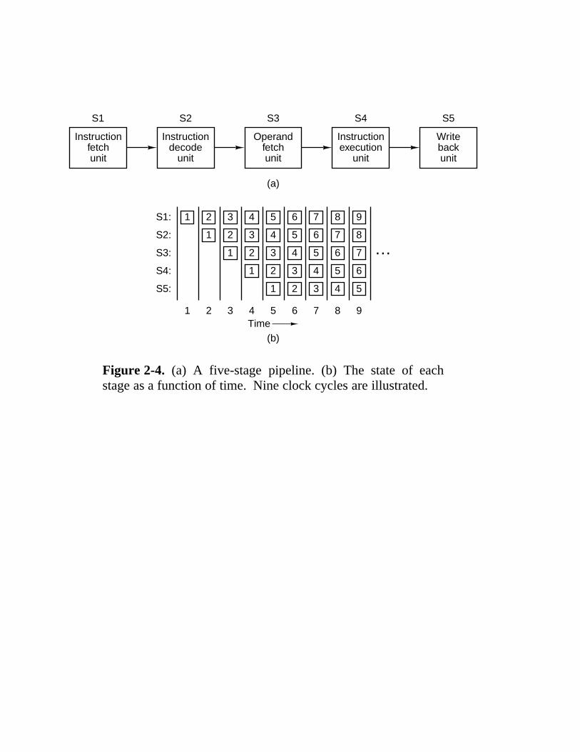
Figure 2-4. (a) A five-stage pipeline. (b) The state of eachstage as a function of time. Nine clock cycles are illustrated.

S1 S2 S3 S4 S5
Instructionfetchunit
Instructiondecode
unit
Operandfetchunit
Instructionexecution
unit
Writebackunit
Instructiondecode
unit
Operandfetchunit
Instructionexecution
unit
Writebackunit
Figure 2-5. (a) Dual five-stage pipelines with a common in-struction fetch unit.

S2 S3 S5
Instructiondecode
unit
Operandfetchunit
LOADWritebackunit
S1
Instructionfetchunit
S4
Floatingpoint
STORE
ALU
ALU
Figure 2-6. A superscalar processor with five functional units.

Control unit
Broadcasts instructions
Processor
Memory
8 × 8 Processor/memory grid
Figure 2-7. An array processor of the ILLIAC IV type.
(a) (b)
CPU
Sharedmemory
Bus
CPU CPU CPU
Local memories
CPU
Sharedmemory
Bus
CPU CPU CPU
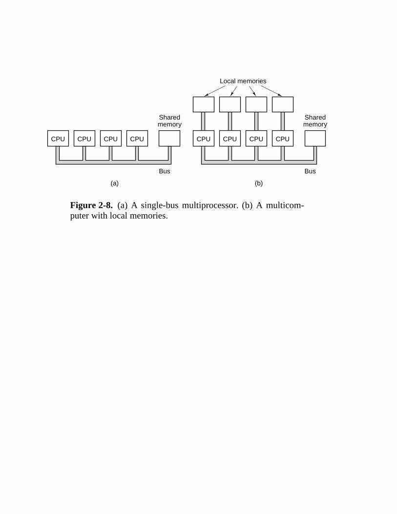
Figure 2-8. (a) A single-bus multiprocessor. (b) A multicom-puter with local memories.
Address 1 Cell
0
(c)
1
2
3
4
5
6
7
8
9
10
11
Address
0
Address
1
2
3
4
5
6
7
0
1
2
3
4
516 bits
(b)
12 bits
(a)
8 bits
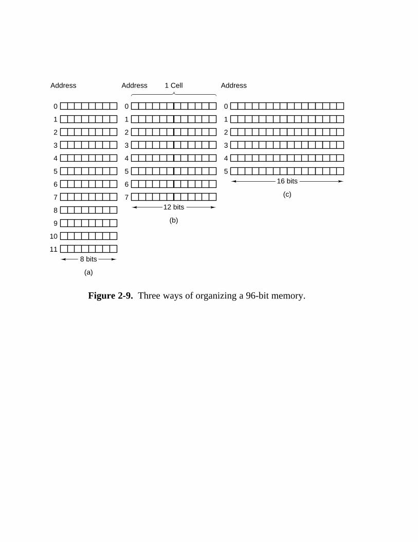
Figure 2-9. Three ways of organizing a 96-bit memory.
2222222222222222222222222222222222Computer Bits/cell2222222222222222222222222222222222
Burroughs B1700 12222222222222222222222222222222222IBM PC 82222222222222222222222222222222222DEC PDP-8 122222222222222222222222222222222222IBM 1130 162222222222222222222222222222222222DEC PDP-15 182222222222222222222222222222222222XDS 940 242222222222222222222222222222222222Electrologica X8 272222222222222222222222222222222222XDS Sigma 9 322222222222222222222222222222222222Honeywell 6180 362222222222222222222222222222222222CDC 3600 482222222222222222222222222222222222CDC Cyber 602222222222222222222222222222222222111111111111111111
111111111111111111
111111111111111111
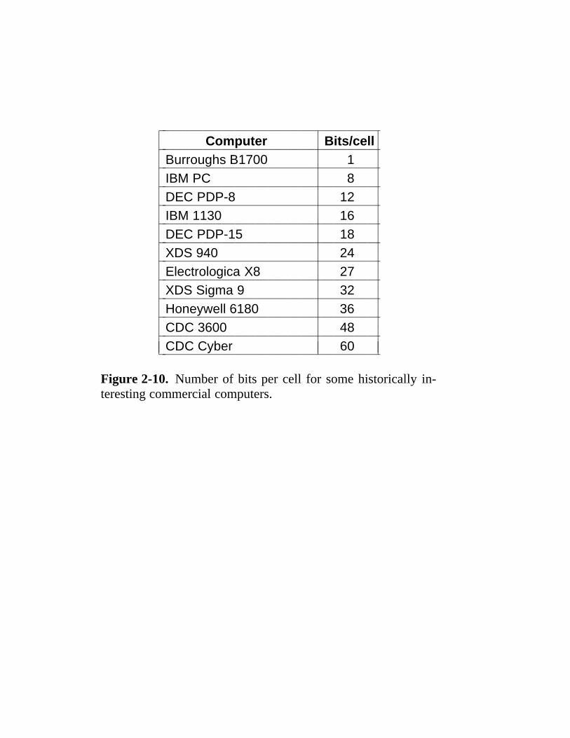
Figure 2-10. Number of bits per cell for some historically in-teresting commercial computers.

Address AddressBig endian
Byte
00
(a)
44
88
1212
0
4
8
12
1
5
9
13
2
6
10
14
3
7
11
15
32-bit word
Little endian
Byte
3
(b)
7
11
15
2
6
10
14
1
5
9
13
0
4
8
12
32-bit word
Figure 2-11. (a) Big endian memory. (b) Little endian memory.

Big endian
(a)
J0 I M
S4 M I T
H8 0 0 0
012 0 0 21
016 0 1 4
Little endian
(b)
J 0M I
T 4I M S
0 80 0 H
0 120 0 21
0 160 1 4
Transfer frombig endian tolittle endian
(c)
JM I
T I M S
0 0 0 H
21 0 0 0
4 1 0 0
Transfer andswap
(d)
J 0I M
S 4M I T
H 80 0 0
0 120 0 21
0 160 1 4
Figure 2-12. (a) A personnel record for a big endian machine.(b) The same record for a little endian machine. (c) The resultof transferring the record from a big endian to a little endian.(d) The result of byte-swapping (c).

22222222222222222222222222222222222222222222222222222Word size Check bits Total size Percent overhead22222222222222222222222222222222222222222222222222222
8 4 12 502222222222222222222222222222222222222222222222222222216 5 21 312222222222222222222222222222222222222222222222222222232 6 38 192222222222222222222222222222222222222222222222222222264 7 71 1122222222222222222222222222222222222222222222222222222
128 8 136 622222222222222222222222222222222222222222222222222222256 9 265 422222222222222222222222222222222222222222222222222222512 10 522 22222222222222222222222222222222222222222222222222222211
1111111111
111111111111
111111111111
111111111111
111111111111
Figure 2-13. Number of check bits for a code that can correcta single error.

B
A
C11
0
0
(a)
B
(b)
Paritybits
A
C11
0
0
0
0
1
(c)
Error
A
B
C1 11
1
0
0
0
Figure 2-14. (a) Encoding of 1100. (b) Even parity added. (c) Error in AC.

Memory word 1111000010101110
01
02
13
04
15
16
17
08
09
010
011
012
113
014
115
116
017
118
119
120
021
Parity bits
Figure 2-15. Construction of the Hamming code for thememory word 1111000010101110 by adding 5 check bits to the16 data bits.

Cache
Bus
Mainmemory
CPU
Figure 2-16. The cache is logically between the CPU andmain memory. Physically, there are several possible places itcould be located.

4-MBmemory
chip
Connector
Figure 2-17. A single inline memory module (SIMM) holding32 MB. Two of the chips control the SIMM.

Registers
Main memory
Cache
Tape
Magnetic disk
Optical disk
Figure 2-18. A five-level memory hierarchy.

Trackwidth is5–10 microns
Width of1 bit is0.1 to 0.2 microns
Directionof armmotion
Diskarm
Read/writehead
Intersector gap
Direction of disk rotation4096 data bits
Preamble
EC
C
4096 data bits
Preamble
ECC1 sector
Figure 2-19. A portion of a disk track. Two sectors are illustrated.

Surface 2Surface 1
Surface 0
Read/write head (1 per surface)
Direction of arm motion Surface 3
Surface 5
Surface 4
Surface 7
Surface 6
Figure 2-20. A disk with four platters.
222222222222222222222222222222222222222222222222222222222222Parameters LD 5.25′′ HD 5.25′′ LD 3.5′′ HD 3.5′′222222222222222222222222222222222222222222222222222222222222
Size (inches) 5.25 5.25 3.5 3.5222222222222222222222222222222222222222222222222222222222222Capacity (bytes) 360K 1.2M 720K 1.44M222222222222222222222222222222222222222222222222222222222222Tracks 40 80 80 80222222222222222222222222222222222222222222222222222222222222Sectors/track 9 15 9 18222222222222222222222222222222222222222222222222222222222222Heads 2 2 2 2222222222222222222222222222222222222222222222222222222222222Rotations/min 300 360 300 300222222222222222222222222222222222222222222222222222222222222Data rate (kbps) 250 500 250 500222222222222222222222222222222222222222222222222222222222222Type Flexible Flexible Rigid Rigid2222222222222222222222222222222222222222222222222222222222221111111111111
1111111111111
1111111111111
1111111111111
1111111111111
1111111111111
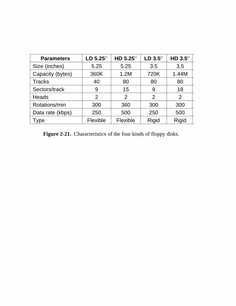
Figure 2-21. Characteristics of the four kinds of floppy disks.

222222222222222222222222222222222222222222222222222222Name Data bits Bus MHz MB/sec222222222222222222222222222222222222222222222222222222
SCSI-1 8 5 5222222222222222222222222222222222222222222222222222222SCSI-2 8 5 5222222222222222222222222222222222222222222222222222222Fast SCSI-2 8 10 10222222222222222222222222222222222222222222222222222222Fast & wide SCSI-2 16 10 20222222222222222222222222222222222222222222222222222222Ultra SCSI 16 20 4022222222222222222222222222222222222222222222222222222211
1111111
111111111
111111111
111111111
111111111
Figure 2-22. Some of the possible SCSI parameters.
P16-19 Strip 12 Strip 17 Strip 18
Strip 12 P16-12 Strip 13 Strip 14
(a)
(b)
(c)
(d)
(e)
(f)
RAID level 0
Strip 8
Strip 4
Strip 0
Strip 9
Strip 5
Strip 1
Strip 10
Strip 6
Strip 2
RAID level 2
Strip 11
Strip 7
Strip 3
Strip 8
Strip 4
Strip 0
Strip 9
Strip 5
Strip 1
Strip 10
Strip 6
Strip 2
Strip 11
Strip 7
Strip 3
Strip 8
Strip 4
Strip 0
Strip 9
Strip 5
Strip 1
Strip 10
Strip 6
Strip 2
Strip 11
Strip 7
Strip 3
Bit 1 Bit 2 Bit 3 Bit 4 Bit 5 Bit 6
RAIDlevel 1
Bit 7
Bit 1 Bit 2 Bit 3 Bit 4
Strip 8
Strip 4
Strip 0
Strip 9
Strip 5
Strip 1
Strip 10
Strip 6
Strip 2
Strip 11
Strip 7
Strip 3
Strip 8
Strip 4
Strip 0
Strip 9
Strip 5
Strip 1
P8-11
Strip 6
Strip 2
Strip 10
P4-7
Strip 3
Strip 19
Strip 15
RAID level 3
RAID level 4
RAID level 5
Parity
P8-11
P4-7
P0-3
Strip 11
Strip 7
P0-3
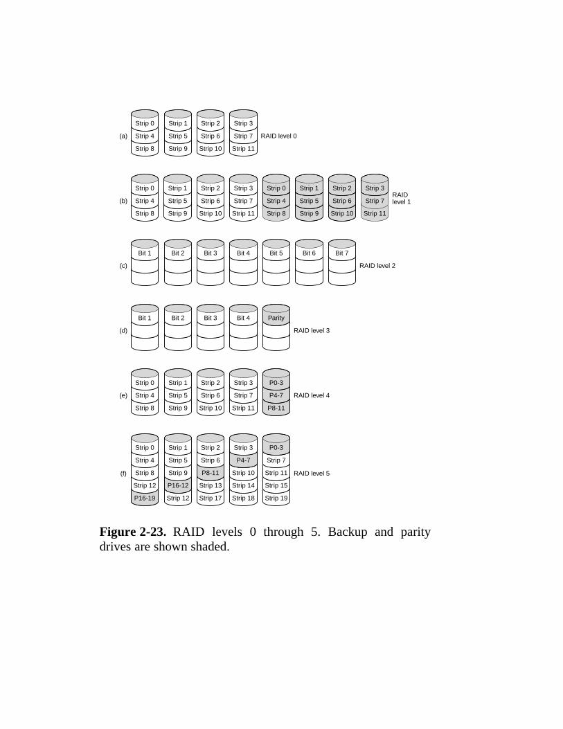
Figure 2-23. RAID levels 0 through 5. Backup and paritydrives are shown shaded.
Spiral groove
Pit
Land
2K block ofuser data
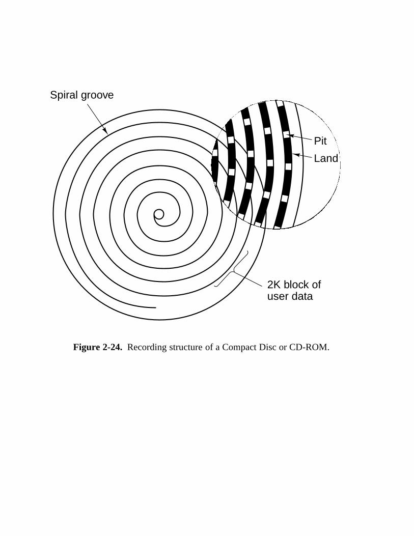
Figure 2-24. Recording structure of a Compact Disc or CD-ROM.

Preamble
Bytes 16
Data
2048 288
ECCMode 1sector
(2352 bytes)
Frames of 588 bits,each containing24 data bytes
Symbols of14 bits each
42 Symbols make 1 frame
98 Frames make 1 sector
…
…
Figure 2-25. Logical data layout on a CD-ROM.
Printed label
Protective lacquerReflective gold layer
layer
Substrate
Directionof motion Lens
Photodetector Prism
Infraredlaserdiode
Dark spot in thedye layer burnedby laser whenwriting1.2 mm
Dye
Polycarbonate
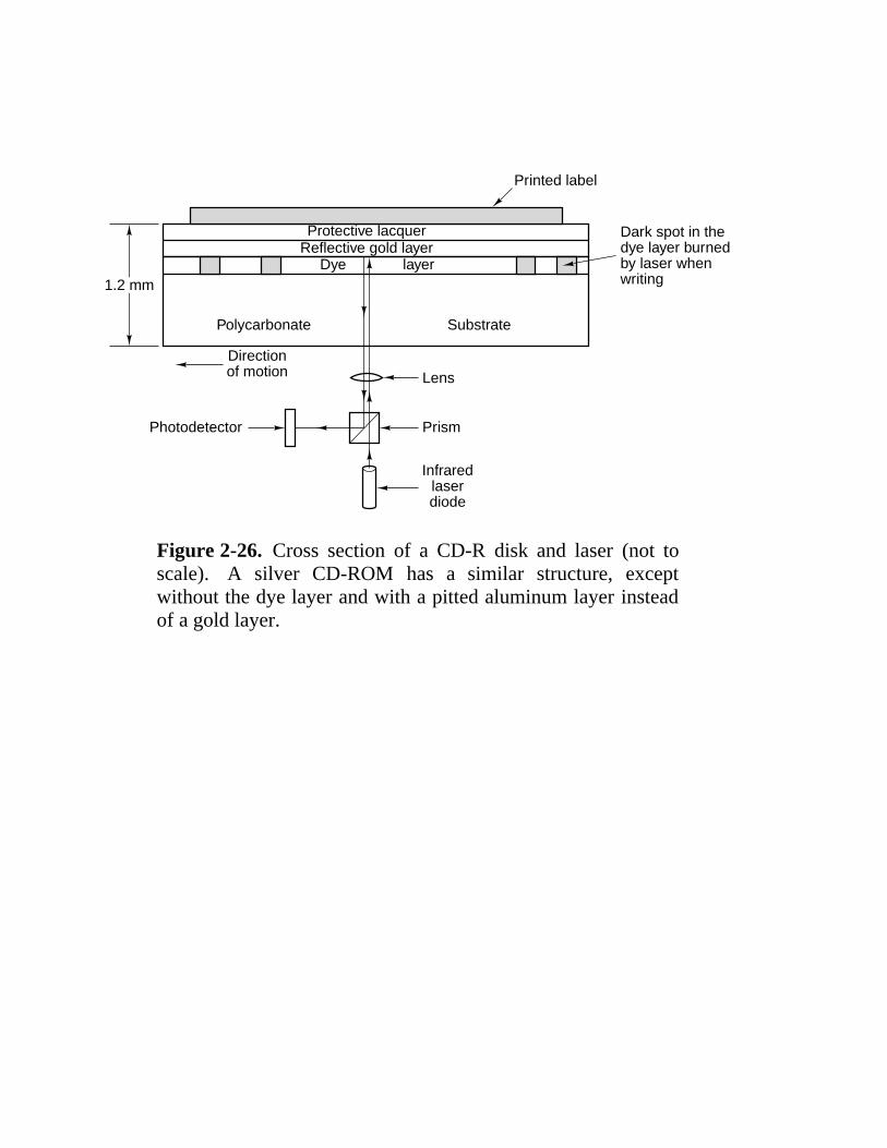
Figure 2-26. Cross section of a CD-R disk and laser (not toscale). A silver CD-ROM has a similar structure, exceptwithout the dye layer and with a pitted aluminum layer insteadof a gold layer.
Polycarbonate substrate 1
Polycarbonate substrate 2
Semireflectivelayer
Semireflectivelayer
Aluminumreflector
Aluminumreflector
0.6 mmSingle-sided
disk
0.6 mmSingle-sided
disk
� � � �� � �� � �� � �� � �� � �� � �� � �� � �
Adhesive layer
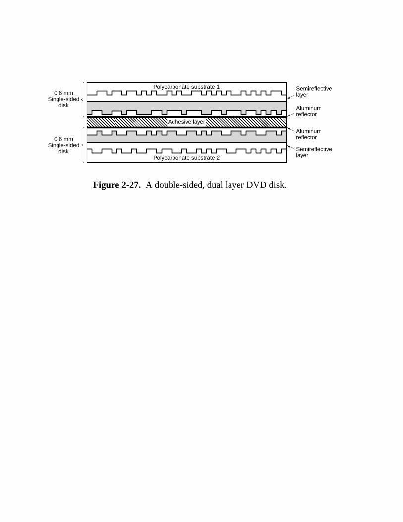
Figure 2-27. A double-sided, dual layer DVD disk.

SCSI controller
Sound card
Modem
Edge connectorCard cage
Figure 2-28. Physical structure of a personal computer.

Monitor
Keyboard Floppydisk drive
Harddisk drive
Harddisk
controller
Floppydisk
controller
Keyboardcontroller
VideocontrollerMemoryCPU
Bus
Figure 2-29. Logical structure of a simple personal computer.

��� �� �� ��
Memory bus
CPU PCIbridge
SCSIcontroller
SCSIdisk
Networkcontroller
Videocontroller
Printercontroller
Soundcard ModemISA
bridge
SCSIscanner
MainmemorySCSI
bus
PCI bus
ISA bus
cache
Figure 2-30. A typical modern PC with a PCI bus and an ISAbus. The modem and sound card are ISA devices; the SCSIcontroller is a PCI device.
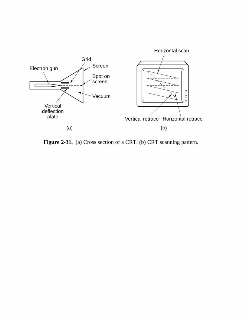
(a) (b)
Electron gun
GridScreen
Spot onscreen
Vacuum
Verticaldeflection
plate
Horizontal scan
Vertical retrace Horizontal retrace
Figure 2-31. (a) Cross section of a CRT. (b) CRT scanning pattern.

(a)(b)
y
z
Rear glass plate
Liquid crystal
Rearelectrode
Rearpolaroid
Front glass plate
Front electrode
Front polaroid
Bright
Dark
Lightsource
Notebook computer
����AACC����ÁÁÃÃ����AACC����ÁÁÃÃ����AACC����ÁÁÃÃ����AACC����ÁÁÃÃ����AACC����ÁÁÃÃ����AACC����ÁÁÃÃ����AACC����ÁÁÃÃ����AACC����ÁÁÃÃ����
Figure 2-32. (a) The construction of an LCD screen. (b) Thegrooves on the rear and front plates are perpendicular to oneanother.

CPU
CharacterAttribute
Analog video signal
Monitor
ABC
Bus
VideoRAM
Mainmemory
Videoboard
A2B2C2
Figure 2-33. Terminal output on a personal computer.
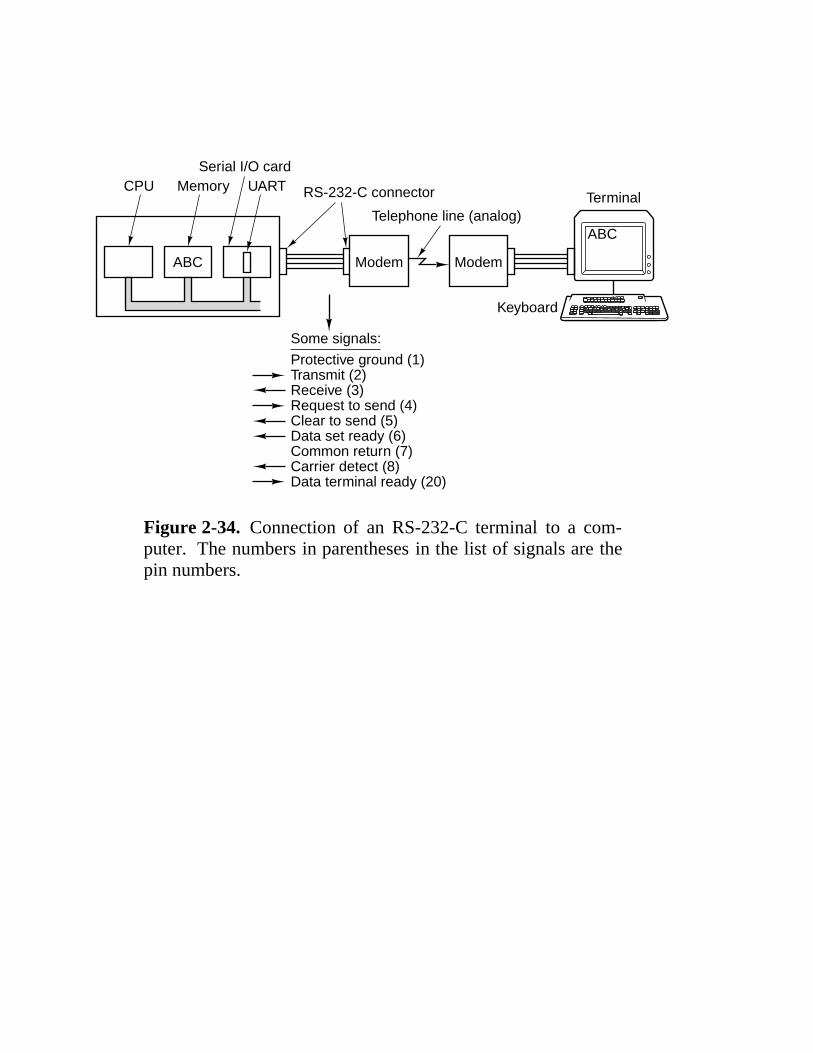
CPU MemorySerial I/O card
UART RS-232-C connector
Telephone line (analog)
Modem ModemABC
Keyboard
Some signals:
Protective ground (1)Transmit (2)Receive (3)Request to send (4)Clear to send (5)Data set ready (6)Common return (7)Carrier detect (8)Data terminal ready (20)
Terminal
ABC
Figure 2-34. Connection of an RS-232-C terminal to a com-puter. The numbers in parentheses in the list of signals are thepin numbers.

Pointer controlled by mouse
Window Menu
Mouse buttons
Mouse
Rubber ball
CutPasteCopy
Figure 2-35. A mouse being used to point to menu items.

(a) (b)
Figure 2-36. (a) The letter ‘‘A’’ on a 5 × 7 matrix. (b) Theletter ‘‘A’’ printed with 24 overlapping needles.

Laser Rotating octagonalmirror
Drum sprayed and charged
Light beamstrikes drum
TonerScraperDischarger
Drum
Blankpaper
Heatedrollers
Stackedoutput
Figure 2-37. Operation of a laser printer.

(a) (b) (c) (d) (e) (f)
Figure 2-38. Halftone dots for various gray scale ranges. (a)0–6. (b) 14–20. (c) 28–34. (d) 56–62. (e) 105–111. (f) 161–167.

(a)
(b)
(c)
(d)
Vol
tage
Time
V1
V20 1 0 0 1 0 1 1 0 0 0 1 0 0
Highamplitude
Lowamplitude
Highfrequency
Lowfrequency
Phase change
Figure 2-39. Transmission of the binary number01001011000100 over a telephone line bit by bit. (a) Two-level signal. (b) Amplitude modulation. (c) Frequency modu-lation. (d) Phase modulation.

ISDN terminal
Customer's equipment Carrier's equipment
ISDNtelephone
ISDNterminal
ISDNalarm
Digitalbit pipe
T U Tocarrier'sinternalnetwork
NT1 ISDNexchange
Figure 2-40. ISDN for home use.


SEC. 2.3 89
2.4 INPUT/OUTPUT
As we mentioned at the start of this chapter, a computer system has threemajor components: the CPU, the memories (primary and secondary), and the I/O(Input/Output) equipment such as printers, scanners, and modems. So far wehave looked at the CPU and the memories. Now it is time to examine the I/Oequipment and how it is connected to the rest of the system.
2.4.1 Buses
Physically, most personal computers and workstations have a structure similarto the one shown in Fig. 2-1. The usual arrangement is a metal box with a largeprinted circuit board at the bottom, called the motherboard (parentboard, for thepolitically correct). The motherboard contains the CPU chip, some slots intowhich DIMM modules can be clicked, and various support chips. It also containsa bus etched along its length, and sockets into which the edge connectors of I/Oboards can be inserted. Sometimes there are two buses, a high-speed one (formodern I/O boards) and a low-speed one (for older I/O boards).
SCSI controller
Sound card
Modem
Edge connectorCard cage
Figure 2-1. Physical structure of a personal computer.
The logical structure of a simple low-end personal computer is shown inFig. 2-2. This one has a single bus used to connect the CPU, memory, and I/Odevices; most systems have two or more buses. Each I/O device consists of twoparts: one containing most of the electronics, called the controller, and one con-taining the I/O device itself, such as a disk drive. The controller is usually con-tained on a board plugged into a free slot, except for those controllers that are notoptional (such as the keyboard), which are sometimes located on the motherboard.Even though the display (monitor) is not an option, the video controller is some-times located on a plug-in board to allow the user to choose between boards withor without graphics accelerators, extra memory, and so on. The controller con-nects to its device by a cable attached to a connector on the back of the box.

90 COMPUTER SYSTEMS ORGANIZATION CHAP. 2
Monitor
Keyboard Floppydisk drive
Harddisk drive
Harddisk
controller
Floppydisk
controller
Keyboardcontroller
VideocontrollerMemoryCPU
Bus
Figure 2-2. Logical structure of a simple personal computer.
The job of a controller is to control its I/O device and handle bus access for it.When a program wants data from the disk for example, it gives a command to thedisk controller, which then issues seeks and other commands to the drive. Whenthe proper track and sector have been located, the drive begins outputting the dataas a serial bit stream to the controller. It is the job of the controller to break thebit stream up into units, and write each unit into memory, as it is assembled. Aunit is typically one or more words. A controller that reads or writes data to orfrom memory without CPU intervention is said to be performing Direct MemoryAccess, better known by its acronym DMA. When the transfer is completed, thecontroller normally causes an interrupt, forcing the CPU to suspend running itscurrent program and start running a special procedure, called an interrupthandler, to check for errors, take any special action needed, and inform theoperating system that the I/O is now finished. When the interrupt handler is fin-ished, the CPU continues with the program that was suspended when the interruptoccurred.
The bus is not only used by the I/O controllers, but also by the CPU for fetch-ing instructions and data. What happens if the CPU and an I/O controller want touse the bus at the same time? The answer is that a chip called a bus arbiterdecides who goes next. In general, I/O devices are given preference over theCPU, because disks and other moving devices cannot be stopped, and forcingthem to wait would result in lost data. When no I/O is in progress, the CPU canhave all the bus cycles for itself to reference memory. However, when some I/Odevice is also running, that device will request and be granted the bus when itneeds it. This process is called cycle stealing and it slows down the computer.
This design worked fine for the first personal computers, since all the com-ponents were roughly in balance. However, as the CPUs, memories, and I/O dev-ices got faster, a problem arose: the bus could no longer handle the loadpresented. On a closed system, such as an engineering workstation, the solution

SEC. 2.4 INPUT/OUTPUT 91
was to design a new and faster bus for the next model. Because nobody evermoved I/O devices from an old model to a new one, this approached worked fine.
However, in the PC world, people often upgraded their CPU but wanted tomove their printer, scanner, and modem to the new system. Also, a huge industryhad grown up around providing a vast range of I/O devices for the IBM PC bus,and this industry had exceedingly little interest in throwing out its entire invest-ment and starting over. IBM learned this the hard way when it brought out thesuccessor to the IBM PC, the PS/2 range. The PS/2 had a new, and faster bus, butmost clone makers continued to use the old PC bus, now called the ISA (IndustryStandard Architecture) bus. Most disk and I/O device makers also continued tomake controllers for it, so IBM found itself in the peculiar situation of being theonly PC maker that was no longer IBM compatible. Eventually, it was forcedback to supporting the ISA bus. As an aside, please note that ISA stands forInstruction Set Architecture in the context of machine levels whereas it stands forIndustry Standard Architecture in the context of buses.
Nevertheless, despite the market pressure not to change anything, the old busreally was too slow, so something had to be done. This situation led to other com-panies developing machines with multiple buses, one of which was the old ISAbus, or its backward-compatible successor, the EISA (Extended ISA) bus. Themost popular of these now is the PCI (Peripheral Component Interconnect)bus. It was designed by Intel, but Intel decided to put all the patents in the publicdomain, to encourage the entire industry (including its competitors) to adopt it.
The PCI bus can be used in many configurations, but a typical one is illus-trated in Fig. 2-3. Here the CPU talks to a memory controller over a dedicatedhigh-speed connection. The controller talks to the memory and to the PCI busdirectly, so CPU-memory traffic does not go over the PCI bus. However, high-bandwidth (i.e., high data rate) peripherals, such as SCSI disks, can connect to thePCI bus directly. In addition, the PCI bus has a bridge to the ISA bus, so that ISAcontrollers and their devices can still be used. A machine of this design wouldtypically contain three or four empty PCI slots and another three or four emptyISA slots, to allow customers to plug in both old ISA I/O cards (usually for slowdevices) and new PCI I/O cards (usually for fast devices).
Many kinds of I/O devices are available today. A few of the more commonones are discussed below.
2.4.2 Terminals
Computer terminals consist of two parts: a keyboard and a monitor. In themainframe world, these parts are often integrated into a single device and attachedto the main computer by a serial line or over a telephone line. In the airline reser-vation, banking, and other mainframe-oriented industries, these devices are still inwidespread use. In the personal computer world, the keyboard and monitor areindependent devices. Either way, the technology of the two parts is the same.

92 COMPUTER SYSTEMS ORGANIZATION CHAP. 2
�� �� ���
Memory bus
CPU PCIbridge
SCSIcontroller
SCSIdisk
Networkcontroller
Videocontroller
Printercontroller
Soundcard ModemISA
bridge
SCSIscanner
MainmemorySCSI
bus
PCI bus
ISA bus
cache
Figure 2-3. A typical modern PC with a PCI bus and an ISA bus. The modemand sound card are ISA devices; the SCSI controller is a PCI device.
Keyboards
Keyboards come in several varieties. The original IBM PC came with a key-board that had a snap-action switch under each key that gave tactile feedback andmade a click with the key was depressed far enough. Nowadays, the cheaper key-boards have keys that just make mechanical contact when depressed. Better oneshave a sheet of elastometric material (a kind of rubber) between the keys and theunderlying printed circuit board. Under each key is a small dome that buckleswhen depressed far enough. A small spot of conductive material inside the domecloses the circuit. Some keyboards have a magnet under each key that passesthrough a coil when struck, thus inducing a current that can be detected. Variousother methods, both mechanical and electromagnetic, are also in use.
On personal computers, when a key is depressed, an interrupt is generated andthe keyboard interrupt handler (a piece of software that is part of the operatingsystem) is started. The interrupt handler reads a hardware register inside the key-board controller to get the number of the key (1 through 102) that was justdepressed. When a key is released, a second interrupt is caused. Thus if a userdepresses the SHIFT key, then depresses and releases the M key, then releases theSHIFT key, the operating system can see that the user wants an upper case ‘‘M’’rather than a lower case ‘‘m.’’ Handling of multikey sequences involving SHIFT,CTRL, and ALT is done entirely in software (including the infamous CTRL-ALT-DEL key sequence that is used to reboot all IBM PCs and clones).

SEC. 2.4 INPUT/OUTPUT 93
CRT Monitors
A monitor is a box containing a CRT (Cathode Ray Tube) and its powersupplies. The CRT contains a gun that can shoot an electron beam against a phos-phorescent screen near the front of the tube, as shown in Fig. 2-4(a). (Color moni-tors have three electron guns, one each for red, green and blue.) During the hor-izontal scan, the beam sweeps across the screen in about 50 µsec, tracing out analmost horizontal line on the screen. Then it executes a horizontal retrace to getback to the left-hand edge in order to begin the next sweep. A device like this thatproduces an image line by line is called a raster scan device.
(a) (b)
Electron gun
GridScreen
Spot onscreen
Vacuum
Verticaldeflection
plate
Horizontal scan
Vertical retrace Horizontal retrace
Figure 2-4. (a) Cross section of a CRT. (b) CRT scanning pattern.
Horizontal sweeping is controlled by a linearly increasing voltage applied tothe horizontal deflection plates placed to the left and right of the electron gun.Vertical motion is controlled by a much more slowly linearly increasing voltageapplied to the vertical deflection plates placed above and below the gun. Aftersomewhere between 400 and 1000 sweeps, the voltages on the vertical and hor-izontal deflection plates are rapidly reversed together to put the beam back in theupper left-hand corner. A full-screen image is normally repainted between 30 and60 times a second. The beam motions are shown in Fig. 2-4(b). Although wehave described CRTs as using electric fields for sweeping the beam across thescreen, many models use magnetic fields instead of electric ones, especially inhigh-end monitors.
To produce a pattern of dots on the screen, a grid is present inside the CRT.When a positive voltage is applied to the grid, the electrons are accelerated, caus-ing the beam to hit the screen and make it glow briefly. When a negative voltageis used, the electrons are repelled, so they do not pass through the grid and thescreen does not glow. Thus the voltage applied to the grid causes the correspond-ing bit pattern to appear on the screen. This mechanism allows a binary electricalsignal to be converted into a visual display consisting of bright and dark spots.
94 COMPUTER SYSTEMS ORGANIZATION CHAP. 2
Flat Panel Displays
CRTs are far too bulky and heavy to be used in notebook computers, so acompletely different technology is needed for their screens. The most commonone is LCD (Liquid Crystal Display) technology. It is highly complex, hasmany variations, and is changing rapidly, so this description will, of necessity, bebrief and greatly simplified.
Liquid crystals are viscous organic molecules that flow like a liquid but alsohave spatial structure, like a crystal. They were discovered by an Austrian botan-ist (Rheinitzer) in 1888, and first applied to displays (e.g., calculators, watches) inthe 1960s. When all the molecules are lined up in the same direction, the opticalproperties of the crystal depend on the direction and polarization of the incominglight. Using an applied electric field, the molecular alignment, hence the opticalproperties, can be changed. In particular, by shining a light through a liquid crys-tal, the intensity of the light exiting from it can be controlled electrically. Thisproperty can be exploited to construct flat panel displays.
An LCD display screen consists of two parallel glass plates between which isa sealed volume containing a liquid crystal. Transparent electrodes are attachedto both plates. A light behind the rear plate (either natural or artificial) illumi-nates the screen from behind. The transparent electrodes attached to each plateused to create electric fields in the liquid crystal. Different parts of the screen getdifferent voltages, to control the image displayed. Glued to the front and rear ofthe screen are polaroids because the display technology requires the use of polar-ized light. The general setup is shown in Fig. 2-5(a).
Although many kinds of LCD displays are in use, we will now consider oneparticular kind of display, the TN (Twisted Nematic) display as an example. Inthis display, the rear plate contains tiny horizontal grooves and the front plate con-tains tiny vertical grooves, as illustrated in Fig. 2-5(b). In the absence of an elec-tric field, the LCD molecules tend to align with the grooves. Since the front andrear alignments differ by 90 degrees, the molecules (and thus the crystal structure)twist from rear to front.
At the rear of the display is a horizontal polaroid. It only allows in horizon-tally polarized light. At the front of the display is a vertical polaroid. It onlyallows vertically polarized light to pass through. If there were no liquid presentbetween the plates, horizontally polarized light let in by the rear polaroid wouldbe blocked by the front polaroid, making the screen uniformly black.
However the twisted crystal structure of the LCD molecules guides the lightas it passes and rotates its polarization, making it come out horizontally. Thus inthe absence of an electric field, the LCD screen is uniformly bright. By applyinga voltage to selected parts of the plate, the twisted structure can be destroyed,blocking the light in those parts.
Two schemes are commonly used for applying the voltage. In a (low-cost)passive matrix display, both electrodes contain parallel wires. In a 640 × 480

SEC. 2.4 INPUT/OUTPUT 95
(a)(b)
y
z
Rear glass plate
Liquid crystal
Rearelectrode
Rearpolaroid
Front glass plate
Front electrode
Front polaroid
Bright
Dark
Lightsource
Notebook computer
��@@��ÀÀ��@@��ÀÀ��@@��ÀÀ��@@��ÀÀ��@@��ÀÀ��@@��ÀÀ��@@��ÀÀ��@@��ÀÀ��
Figure 2-5. (a) The construction of an LCD screen. (b) The grooves on the rearand front plates are perpendicular to one another.
display, for example, the rear electrode might have 640 vertical wires and thefront one might have 480 horizontal ones. By putting a voltage on one of the vert-ical wires and then pulsing one of the horizontal ones, the voltage at one selectedpixel position can be changed, making it go dark briefly. By repeating this pulsewith the next pixel and then the next one, a dark scan line can be painted, analo-gous to how a CRT works. Normally, the entire screen is painted 60 times asecond to fool the eye into thinking there is a constant image there, again, thesame way as a CRT.
The other scheme in widespread use is the active matrix display. It is con-siderably more expensive but it gives a better image so it is winning ground.Instead of just having two sets of perpendicular wires, it has a tiny switching ele-ment at each pixel position on one of the electrodes. By turning these on and off,an arbitrary voltage pattern can be created across the screen, allowing for an arbi-trary bit pattern.
So far we have described how a monochrome display works. Suffice it to saythat color displays uses the same general principles as monochrome displays, butthat the details are a great deal more complicated. Optical filters are used toseparate the white light into red, green, and blue components at each pixel posi-tion so these can be displayed independently. Every color can be built up from alinear superposition of these three primary colors.

96 COMPUTER SYSTEMS ORGANIZATION CHAP. 2
Character-Map Terminals
Three kinds of terminals are in common use: character-map terminals, bit-map terminals, and RS-232-C terminals. They all can use any keyboard type, butthey differ in the way the computer communicates with them and how the outputis handled. We will now briefly describe each kind.
On a personal computer, there are two ways to organize the output to thescreen: a character map and a bit map. Figure 2-6 shows how a character map isused to display output on the monitor. (The keyboard is treated as a completelyseparate device.) On the serial communication board is a chunk of memory,called the video memory, as well as some electronics for accessing the bus andgenerating video signals.
CPU
CharacterAttribute
Analog video signal
Monitor
ABC
Bus
VideoRAM
Mainmemory
Videoboard
A2B2C2
Figure 2-6. Terminal output on a personal computer.
To display characters, the CPU copies them to the video memory in alternatebytes. Associated with each character is an attribute byte that describes how thatcharacter is to be displayed. Attributes can include its color, intensity, whether itis blinking, and so on. Thus a screen image of 25 × 80 characters requires 4000bytes of video memory, 2000 for the characters and 2000 for the attributes. Mostboards have more memory to hold multiple screen images.
The job of the video board is to repeatedly fetch characters from the videoRAM and generate the necessary signal to drive the monitor. An entire line ofcharacters is fetched at once so the individual scan lines can be computed. Thissignal is a high-frequency analog signal that controls the scanning of the electronbeam that paints the characters on the screen. Because the board outputs a videosignal, the monitor must be within a few meters of the computer to prevent distor-tion.
Bit-map Terminals
A variation on this idea is to have the screen not be regarded as a 25 × 80 ar-ray of characters, but as an array of picture elements, called pixels. Each pixel iseither on or off. It represents one bit of information. On personal computers the
SEC. 2.4 INPUT/OUTPUT 97
screen may contain as few as 640 × 480 pixels, but more commonly 800 × 600 ormore. On engineering workstations, the screen is typically 1280 × 960 pixels ormore. Terminals using a bit map rather than a character map are called bit-mapterminals. All modern video boards can operate either as character-map termi-nals or bit-map terminals, under software control.
The same general idea is used as in Fig. 2-6, except that the video RAM isjust seen as a big bit array. The software can set any pattern it wants there, andthat is displayed instantly. To draw characters, the software might decide to allo-cate, for example, a 9 by 14 rectangle for each character and fill in the necessarybits to make the character appear. This approach allows the software to createmultiple fonts and intermix them at will. All the hardware does is display the bitarray. For color displays, each pixel is 8, 16, or 24 bits.
Bit-map terminals are commonly used to support displays containing severalwindows. A window is an area of the screen used by one program. With multiplewindows, it is possible to have several programs running at the same time, eachone displaying its results independent of the other ones.
Although bit-map terminals are highly flexible, they have two major disad-vantages. First, they require a considerable amount of video RAM. The mostcommon sizes these days are 640 × 480 (VGA), 800 × 600 (SVGA), 1024 × 768(XVGA), and 1280 × 960). Notice that all of these have an aspect ratio(width:height) of 4:3, to conform to the current ratio for television sets. To gettrue color, 8 bits are needed for each of the three primary colors, or 3 bytes/pixel.Thus a 1024 × 768 display, requires 2.3 MB of video RAM.
As a result of this large requirement, some computers compromise by usingan 8-bit number to indicate the color desired. This number is then used as anindex into a hardware table, called the color palette that contains 256 entries,each holding a 24-bit RGB value. Such a design, called indexed color, reducesthe memory video RAM memory requirements by 2/3, but allows only 256 colorson the screen at once. Usually, each window on the screen has its own mapping,but with only one hardware color palette, often when multiple windows arepresent on the screen, only the current one has its colors rendered correctly.
The second disadvantage of a bit-map display is performance. Once applica-tion programmers realize that they can control every pixel in both space and time,they want to do it. Although data can be copied from the video RAM to the moni-tor without going over the main system bus, getting data into the video RAM doesuse the system bus. To display full-screen, full-color multimedia on a 1024 × 768display requires copying 2.3 MB of data to the video RAM for every frame. Forfull-motion video, a rate of at least 25 frame/sec is needed, for a total data rate of57.6 MB/sec. This load is far more than what the (E)ISA bus can handle, sohigh-performance video cards on IBM PCs need to be PCI cards, and even then,major compromises are required.
A related performance problem is how to scroll the screen. One way is copy-ing all the bits in software, but doing this puts a gigantic load on the CPU. Not
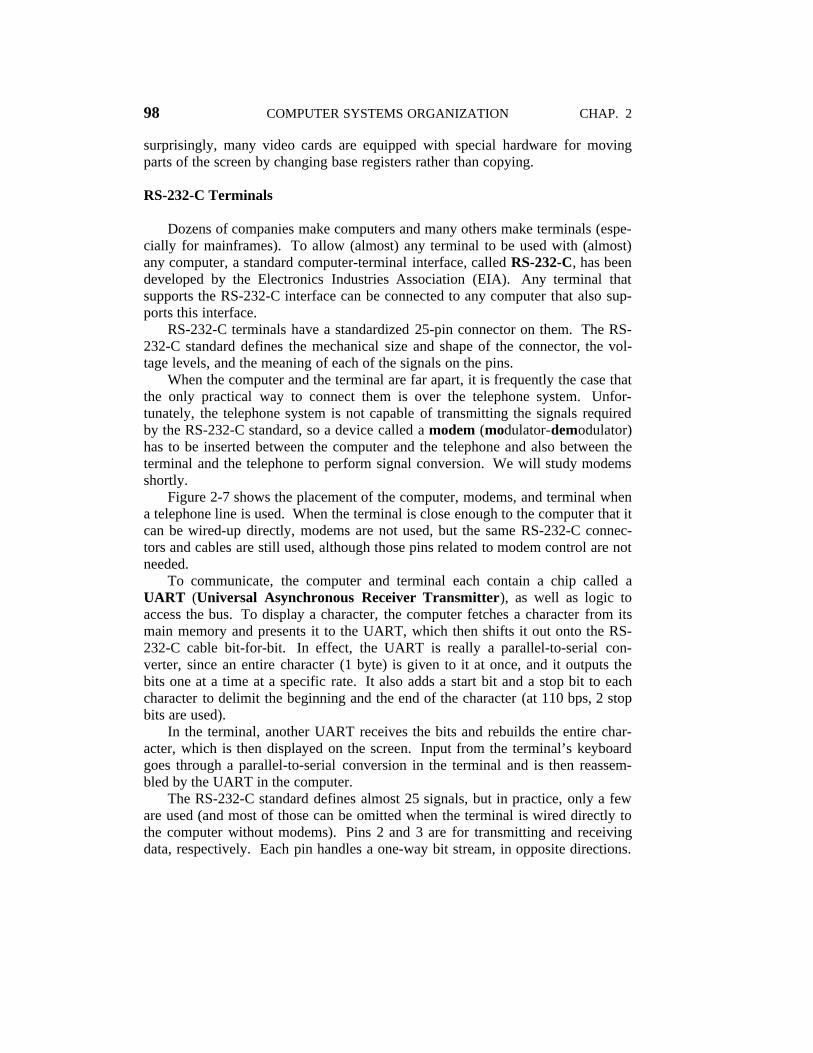
98 COMPUTER SYSTEMS ORGANIZATION CHAP. 2
surprisingly, many video cards are equipped with special hardware for movingparts of the screen by changing base registers rather than copying.
RS-232-C Terminals
Dozens of companies make computers and many others make terminals (espe-cially for mainframes). To allow (almost) any terminal to be used with (almost)any computer, a standard computer-terminal interface, called RS-232-C, has beendeveloped by the Electronics Industries Association (EIA). Any terminal thatsupports the RS-232-C interface can be connected to any computer that also sup-ports this interface.
RS-232-C terminals have a standardized 25-pin connector on them. The RS-232-C standard defines the mechanical size and shape of the connector, the vol-tage levels, and the meaning of each of the signals on the pins.
When the computer and the terminal are far apart, it is frequently the case thatthe only practical way to connect them is over the telephone system. Unfor-tunately, the telephone system is not capable of transmitting the signals requiredby the RS-232-C standard, so a device called a modem (modulator-demodulator)has to be inserted between the computer and the telephone and also between theterminal and the telephone to perform signal conversion. We will study modemsshortly.
Figure 2-7 shows the placement of the computer, modems, and terminal whena telephone line is used. When the terminal is close enough to the computer that itcan be wired-up directly, modems are not used, but the same RS-232-C connec-tors and cables are still used, although those pins related to modem control are notneeded.
To communicate, the computer and terminal each contain a chip called aUART (Universal Asynchronous Receiver Transmitter), as well as logic toaccess the bus. To display a character, the computer fetches a character from itsmain memory and presents it to the UART, which then shifts it out onto the RS-232-C cable bit-for-bit. In effect, the UART is really a parallel-to-serial con-verter, since an entire character (1 byte) is given to it at once, and it outputs thebits one at a time at a specific rate. It also adds a start bit and a stop bit to eachcharacter to delimit the beginning and the end of the character (at 110 bps, 2 stopbits are used).
In the terminal, another UART receives the bits and rebuilds the entire char-acter, which is then displayed on the screen. Input from the terminal’s keyboardgoes through a parallel-to-serial conversion in the terminal and is then reassem-bled by the UART in the computer.
The RS-232-C standard defines almost 25 signals, but in practice, only a feware used (and most of those can be omitted when the terminal is wired directly tothe computer without modems). Pins 2 and 3 are for transmitting and receivingdata, respectively. Each pin handles a one-way bit stream, in opposite directions.

SEC. 2.4 INPUT/OUTPUT 99
CPU MemorySerial I/O card
UART RS-232-C connector
Telephone line (analog)
Modem ModemABC
Keyboard
Some signals:
Protective ground (1)Transmit (2)Receive (3)Request to send (4)Clear to send (5)Data set ready (6)Common return (7)Carrier detect (8)Data terminal ready (20)
Terminal
ABC
Figure 2-7. Connection of an RS-232-C terminal to a computer. The numbersin parentheses in the list of signals are the pin numbers.
When the terminal or computer is powered up, it asserts (i.e., sets to 1) the DataTerminal Ready signal to inform the modem that it is on. Similarly, the modemasserts Data Set Ready to signal its presence. When the terminal or computerwants to send data, it asserts Request to Send to ask permission. If the modem iswilling to grant that permission, it asserts Clear to Send as a response. Other pinsare used for various status, testing, and timing functions.
2.4.3 Mice
As time goes on, computers are being used by people with less expertise inhow computers work. Computers of the ENIAC generation were used only by thepeople who built them. In the 1950s, computers were only used by highly-skilledprofessional programmers. Now, computers are widely used by people who needto get some job done and do not know (or even want to know) much about howcomputers work or how they are programmed.
In the old days, most computers had command line interfaces, to which userstyped commands. Since people who are not computer specialists often perceivedcommand line interfaces as user-unfriendly, if not downright hostile, many com-puter vendors developed point-and-click interfaces, such as the Macintosh andWindows. Using this model requires having a way to point at the screen. Themost common way of allowing users to point at the screen is with a mouse.
A mouse is a small plastic box that sits on the table next to the keyboard.When it is moved around on the table, a little pointer on the screen moves too,
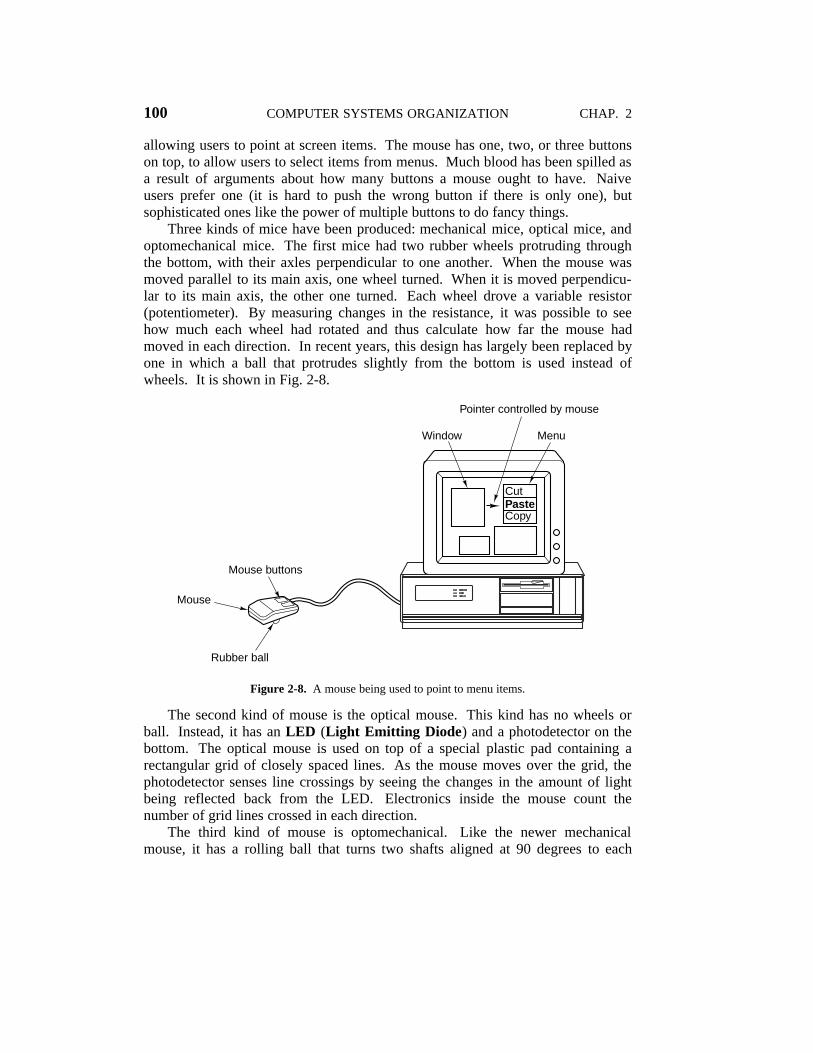
100 COMPUTER SYSTEMS ORGANIZATION CHAP. 2
allowing users to point at screen items. The mouse has one, two, or three buttonson top, to allow users to select items from menus. Much blood has been spilled asa result of arguments about how many buttons a mouse ought to have. Naiveusers prefer one (it is hard to push the wrong button if there is only one), butsophisticated ones like the power of multiple buttons to do fancy things.
Three kinds of mice have been produced: mechanical mice, optical mice, andoptomechanical mice. The first mice had two rubber wheels protruding throughthe bottom, with their axles perpendicular to one another. When the mouse wasmoved parallel to its main axis, one wheel turned. When it is moved perpendicu-lar to its main axis, the other one turned. Each wheel drove a variable resistor(potentiometer). By measuring changes in the resistance, it was possible to seehow much each wheel had rotated and thus calculate how far the mouse hadmoved in each direction. In recent years, this design has largely been replaced byone in which a ball that protrudes slightly from the bottom is used instead ofwheels. It is shown in Fig. 2-8.
Pointer controlled by mouse
Window Menu
Mouse buttons
Mouse
Rubber ball
CutPasteCopy
Figure 2-8. A mouse being used to point to menu items.
The second kind of mouse is the optical mouse. This kind has no wheels orball. Instead, it has an LED (Light Emitting Diode) and a photodetector on thebottom. The optical mouse is used on top of a special plastic pad containing arectangular grid of closely spaced lines. As the mouse moves over the grid, thephotodetector senses line crossings by seeing the changes in the amount of lightbeing reflected back from the LED. Electronics inside the mouse count thenumber of grid lines crossed in each direction.
The third kind of mouse is optomechanical. Like the newer mechanicalmouse, it has a rolling ball that turns two shafts aligned at 90 degrees to each

SEC. 2.4 INPUT/OUTPUT 101
other. The shafts are connected to encoders that have slits through which lightcan pass. As the mouse moves, the shafts rotate, and light pulses strike the detec-tors whenever a slit comes between an LED and its detector. The number ofpulses detected is proportional to the amount of motion.
Although mice can be set up in various ways, a common arrangement is tohave the mouse send a sequence of 3 bytes to the computer every time the mousemoves a certain minimum distance (e.g., 0.01 inch), sometimes called a mickey.Usually, these characters come in on a serial line, one bit at time. The first bytecontains a signed integer telling how many units the mouse has moved in the x-direction in the last 100 msec. The second byte gives the same information for ymotion. The third byte contains the current state of the mouse buttons. Some-times 2 bytes are used for each coordinate.
Low-level software in the computer accepts this information as it comes inand converts the relative movements sent by the mouse to an absolute position. Itthen displays an arrow on the screen at the position corresponding to where themouse is. When the arrow points at the proper item, the user clicks a mouse but-ton, and the computer can then figure out which item has been selected from itsknowledge of where the arrow is on the screen.
2.4.4 Printers
Having prepared a document or fetched a page from the World Wide Web,users often want to print it, so all computers can be equipped with a printer. Inthis section we will describe some of the more common kinds of monochrome(i.e., black and white) and color printers.
Monochrome Printers
The cheapest kind of printer is the matrix printer, in which a print head con-taining between 7 and 24 electromagnetically activatable needles is scannedacross each print line. Low-end printers have seven needles, for printing, say, 80characters in a 5 × 7 matrix across the line. In effect, the print line then consistsof 7 horizontal lines, each consisting of 5 × 80 = 400 dots. Each dot can beprinted or not printed, depending on the characters to be printed. Figure 2-9(a)illustrates the letter ‘‘A’’ printed on a 5 × 7 matrix.
The print quality can be increased by two techniques: using more needles andhaving the circles overlap. Figure 2-9(b) shows an ‘‘A’’ printed using 24 needlesthat produce overlapping dots. Usually, multiple passes over each scan line arerequired to produce overlapping dots, so increased quality goes hand in hand withslower printing rates. Most matrix printers can operate in several modes, offeringdifferent trade-offs between print quality and speed.
Matrix printers are cheap (especially in terms of consumables) and highly reli-able, but slow, noisy, and poor at graphics. They have three main uses in current

102 COMPUTER SYSTEMS ORGANIZATION CHAP. 2
(a) (b)
Figure 2-9. (a) The letter ‘‘A’’ on a 5 × 7 matrix. (b) The letter ‘‘A’’ printedwith 24 overlapping needles.
systems. First, they are popular for printing on large (> 30 cm) preprinted forms.Second, they are good at printing on small pieces of paper, such as cash registerreceipts, ATM machine or credit card transaction slips, or airline boarding passes.Third, for printing on multipart continuous forms with carbon paper embeddedbetween the copies, they are usually the cheapest technology.
For low-cost home printing, inkjet printers are a favorite. The movable printhead, which holds an ink cartridge, is swept horizontally across the paper whileink is sprayed from its tiny nozzles. Inside each nozzle, an ink droplet is electri-cally heated to the boiling point until it explodes. The only place the ink can go isout the front of the nozzle onto the paper. The nozzle is then cooled and theresulting vacuum sucks in another ink droplet. The speed of the printer is limitedby how fast the boil/cool cycle can be repeated. Inkjet printers typically haveresolutions of 300 dpi (dots per inch) to 720 dpi, although 1440 dpi inkjetprinters are also available. They are cheap, quiet, and have good quality, althoughthey are also slow, use expensive ink cartridges, and produce ink-soaked output.
Probably the most exciting development in printing since Johann Gutenberginvented movable type in the fifteenth century is the laser printer. This devicecombines a high quality image, excellent flexibility, good speed, and moderatecost into a single peripheral. Laser printers use almost the same technology asphotocopy machines. In fact, many companies make devices that combine copy-ing and printing (and sometimes fax as well).
The basic technology is illustrated in Fig. 2-10. The heart of the printer is arotating precision drum (or in some high-end systems, a belt). At the start of eachpage cycle, it is charged up to about 1000 volts and coated with a photosensitivematerial. Then light from a laser is scanned along the length of the drum muchlike the electron beam in a CRT, only instead of achieving the horizontal deflec-tion using a voltage, a rotating octagonal mirror is used to scan the length of the

SEC. 2.4 INPUT/OUTPUT 103
drum. The light beam is modulated to produce a pattern of light and dark spots.The spots where the beam hits lose their electrical charge.
Laser Rotating octagonalmirror
Drum sprayed and charged
Light beamstrikes drum
TonerScraperDischarger
Drum
Blankpaper
Heatedrollers
Stackedoutput
Figure 2-10. Operation of a laser printer.
After a line of dots has been painted, the drum rotates a fraction of a degree toallow the next line to be painted. Eventually, the first line of dots reaches thetoner, a reservoir of an electrostatically sensitive black powder. The toner isattracted to those dots that are still charged, thus forming a visual image of thatline. A little later in the transport path, the toner-coated drum is pressed againstthe paper, transferring the black powder to the paper. The paper is then passedthrough heated rollers to fuse the toner to the paper permanently, fixing the image.Later in its rotation, the drum is discharged and scraped clean of any residualtoner, preparing it for being charged and coated again for the next page.
That this process is an exceedingly complex combination of physics, chemis-try, mechanical engineering, and optical engineering hardly needs to be said.Nevertheless, complete assemblies, called print engines, are available fromseveral vendors. Laser printer manufacturers combine the print engines with theirown electronics and software to make a complete printer. The electronics consistsof a fast CPU along with megabytes of memory to hold a full-page bit map andnumerous fonts, some of them built in and some of them downloadable. Mostprinters accept commands that describe the pages to be printed (as opposed tosimply accepting bit maps prepared by the main CPU). These commands aregiven in languages such as HP’s PCL and Adobe’s PostScript.
Laser printers at 600 dpi and up can do a reasonable job of printing black andwhite photographs but the technology is trickier than it might at first appear. Con-sider a photograph scanned in at 600 dpi that is to be printed on a 600 dpi printer.

104 COMPUTER SYSTEMS ORGANIZATION CHAP. 2
The scanned image contains 600 × 600 pixels/inch, each one consisting of a grayvalue from 0 (white) to 255 (black). The printer can also print 600 dpi, but eachprinted pixel is either black (toner present) or white (no toner present). Grayvalues cannot be printed.
The usual solution to printing images with gray values is to use halftoning,the same as commercially printed posters. The image is broken up into halftonecells, each typically 6 × 6 pixels. Each cell can contain between 0 and 36 blackpixels. The eye perceives a cell with many pixels as darker than one with fewerpixels. Gray values in the range 0 to 255 are represented by dividing this rangeinto 37 zones. Values from 0 to 6 are in zone 0, values from 7 to 13 are in zone 1,and so on (zone 36 is slightly smaller than the others because 37 does not divide256 exactly). Whenever a gray value in zone 0 is encountered, its halftone cell onthe paper is left blank, as illustrated in Fig. 2-11(a). A zone 1 value is printed as 1black pixel. A zone 2 value is printed as 2 black pixels, as shown in Fig. 2-11(b).Other zone values are shown in Fig. 2-11(c)-(f). Of course, taking a photographscanned at 600 dpi and halftoning this way reduces the effective resolution to 100cells/inch, called the halftone screen frequency , conventionally measured in lpi(lines per inch).
(a) (b) (c) (d) (e) (f)
Figure 2-11. Halftone dots for various gray scale ranges. (a) 0–6. (b) 14–20. (c)28–34. (d) 56–62. (e) 105–111. (f) 161–167.
Color Printers
Color images can be viewed in one of two ways: transmitted light andreflected light. Transmitted light images, such as those produced on CRT moni-tors, are built up from the linear superposition of the three additive primary colors,red, green, and blue. Reflected light images, such as color photographs and pic-tures in glossy magazines, absorb certain wavelengths of light and reflect the rest.These are built up from a linear superposition of the three subtractative primarycolors, cyan (all red absorbed), yellow (all blue absorbed), and magenta (all greenabsorbed). In theory, every color can be produced by mixing cyan, yellow, andmagenta ink. In practice it is difficult to get the inks pure enough to absorb alllight and produce a true black. For this reason, nearly all color printing systemsuse four inks: cyan, yellow, magenta, and black. These systems are calledCYMK printers (K is for blacK, to avoid confusion with Blue). Monitors, incontrast, use transmitted light and the RGB system for producing colors.

SEC. 2.4 INPUT/OUTPUT 105
The complete set of colors that a display or printer can produce is called itsgamut. No device has a gamut that matches the real world, since at best eachcolor comes in 256 intensities, giving only 16,777,216 discrete colors. Imperfec-tions in the technology reduce the total more, and the remaining ones are notalways uniformly spaced over the color spectrum. Furthermore, color perceptionhas a lot to do with how the rods and cones in the human retina work, and not justthe physics of light.
As a consequence of the above observations, converting a color image thatlooks fine on the screen to an identical printed one is far from trivial. Among theproblems are
1. Color monitors use transmitted light; color printers use reflected light.
2. CRTs produce 256 intensities per color; color printers must halftone.
3. Monitors have a dark background; paper has a light background.
4. The RGB and CMYK gamuts are different.
Getting printed color images to match real life (or even to match screen images)requires device calibration, sophisticated software, and considerable expertise onthe part of the user.
Five technologies are in common use for color printing, all of them based onthe CMYK system. At the low end are color ink jet printers. They work the sameway as monochrome ink jet printers, but with four cartridges (for C, M, Y, and K)instead of one. They give good results for color graphics and passable results forphotographs at modest cost (the printers are cheap but the ink cartridges are not).
For best results, special ink and paper should be used. Two kinds of ink exist.Dye-based inks consist of colored dyes dissolved in a fluid carrier. They givebright colors and flow easily. Their main disadvantage is that they fade whenexposed to ultraviolet light, such as that contained in sunlight. Pigment-basedink contains solid particles of pigment suspended in a fluid carrier that evaporatesfrom the paper, leaving the pigment behind. They do not fade in time but are notas bright as dye-based inks and the pigment particles have a tendency to clog thenozzles, requiring periodic cleaning. Coated or glossy paper is required for print-ing photographs. These kinds of paper have been specially designed to hold theink droplets and not let them spread out.
A step up from ink jet printers leads to the solid ink printers. These acceptfour solid blocks of a special waxy ink which are then melted into hot ink reser-voirs. Startup times of these printers can be as much as 10 minutes, while the inkblocks are melting. The hot ink is sprayed onto the paper, where it solidifies andis fused with the paper by forcing it between two hard rollers
The third kind of color printer is the color laser printer. It works like itsmonochrome cousin, except that separate C, Y, M, and K images are laid downand transferred to a roller using four different toners. Since the full bit map is

106 COMPUTER SYSTEMS ORGANIZATION CHAP. 2
generally produced in advance, a 1200 × 1200 dpi image for a page containing 80square inches needs 115 million pixels. With 4 bits/pixels, the printer needs 55MB just for the bit map, exclusive of memory for the internal processors, fonts,etc. This requirement makes color laser printers expensive, but printing is fast,the quality is high, and the images are stable over time.
The fourth kind of color printer is the wax printer. It has a wide ribbon offour-color wax that is segmented into page-size bands. Thousands of heating ele-ments melt the wax as the paper moves under it. The wax is fused to the paper inthe form of pixels using the CMYK system. Wax printers used to be the maincolor printing technology, but they are being replaced by the other kinds, whichhave cheaper consumables.
The fifth kind of color printer is the dye sublimation printer. Although ithas Freudian undertones, sublimation is the scientific name for a solid changinginto a gas without passing through the liquid state. Dry ice (frozen carbon diox-ide) is a well-known material that subliminates. In a dye sublimation printer, acarrier containing the CMYK dyes passes over a thermal print head containingthousands of programmable heating elements. The dyes are vaporized instantlyand absorbed by a special paper close by. Each heating element can produce 256different temperatures. The higher the temperature, the more dye that is depositedand the more intense the color. Unlike all the other color printers, nearly continu-ous colors are possible for each pixel, so no halftoning is needed. Small snapshotprinters often use the dye sublimation process to produce highly realistic photo-graphic images on special (and expensive) paper.
2.4.5 Modems
With the growth of computer usage in the past years, it is common for onecomputer to need to communicate with another one. For example, many peoplehave personal computers at home that they use for communicating with their com-puter at work, with an Internet Service Provider, or with a home banking system.All these applications use the telephone to provide the underlying communication.
However, a raw telephone line is not suitable for transmitting computer sig-nals, which generally represent a 0 as 0 volts and a 1 as 3 to 5 5 volts as shown inFig. 2-12(a). Two-level signals suffer considerable distortion when transmittedover a voice-grade telephone line, thereby leading to transmission errors. A puresine wave signal at a frequency of 1000 to 2000 Hz, called a carrier, can betransmitted with relatively little distortion, however, and this fact is exploited asthe basis of most telecommunication systems.
Because the pulsations of a sine wave are completely predictable, a pure sinewave transmits no information at all. However, by varying the amplitude, fre-quency, or phase, a sequence of 1s and 0s can be transmitted, as shown in Fig. 2-12. This process is called modulation. In amplitude modulation [see Fig. 2-12(b)], two different voltage levels are used, for 0 and 1, respectively. A person

SEC. 2.4 INPUT/OUTPUT 107
(a)
(b)
(c)
(d)
Vol
tage
Time
V1
V20 1 0 0 1 0 1 1 0 0 0 1 0 0
Highamplitude
Lowamplitude
Highfrequency
Lowfrequency
Phase change
Figure 2-12. Transmission of the binary number 01001011000100 over a tele-phone line bit by bit. (a) Two-level signal. (b) Amplitude modulation.(c) Frequency modulation. (d) Phase modulation.
listening to digital data transmitted at a very low data rate would hear a loud noisefor a 1 and no noise for a 0.
In frequency modulation [see Fig. 2-12(c)], the voltage level is constant butthe carrier frequency is different for 1 and 0. A person listening to frequencymodulated digital data would hear two tones, corresponding to 0 and 1. Fre-quency modulation is often referred to as frequency shift keying.
In simple phase modulation [see Fig. 2-12(d)], the amplitude and frequencydo not change, but the phase of the carrier is reversed 180 degrees when the dataswitch from 0 to 1 or 1 to 0. In more sophisticated phase-modulated systems, atthe start of each indivisible time interval, the phase of the carrier is abruptlyshifted by 45, 135, 225, or 315 degrees, to allow 2 bits per time interval, calleddibit phase encoding. For example, a phase shift of 45 degrees could represent00, a phase shift of 135 degrees could represent 01, and so on. Other schemes, fortransmitting 3 or more bits per time interval also exist. The number of time inter-vals (i.e., the number of potential signal changes per second) is baud rate. With 2or more bits per interval, the bit rate will exceed the baud rate. Many people con-fuse these two terms.
If the data to be transmitted consist of a series of 8-bit characters, it would bedesirable to have a connection capable of transmitting 8 bits simultaneously—thatis, eight pairs of wires. Because voice-grade telephone lines provide only one
108 COMPUTER SYSTEMS ORGANIZATION CHAP. 2
channel, the bits must be sent serially, one after another (or in groups of two ifdibit encoding is being used). The device that accepts characters from a computerin the form of two-level signals, one bit at a time, and transmits the bits in groupsof one or two, in amplitude-, frequency-, or phase-modulated form, is the modem.To mark the start and end of each character, an 8-bit character is normally sentpreceded by a start bit and followed by a stop bit, making 10 bits in all.
The transmitting modem sends the individual bits within one character atregularly-spaced time intervals. For example, 9600 baud implies one signalchange every 104 µsec. A second modem at the receiving end is used to convert amodulated carrier to a binary number. Because the bits arrive at the receiver atregularly-spaced intervals, once the receiving modem has determined the start ofthe character, its clock tells it when to sample the line to read the incoming bits.
Modern modems operate at data rates ranging from 28,800 bits/sec to 57,600bits/sec, usually at much lower baud rates. They use a combination of techniquesto send multiple bits per baud, modulating the amplitude, frequency, and phase.Nearly all of them are full-duplex, meaning they can transmit in both directions atthe same time (using different frequencies). Modems or transmission lines thatcan only transmit in one direction at a time (like a single-track railroad that canhandle north-bound trains or south-bound trains but not at the same time) arecalled half-duplex. Lines that can only transmit in one direction are simplex.
ISDN
In the early 1980s, the European PTTs (Post, Telephone, and TelegraphAdministrations) developed a standard for digital telephony called ISDN(Integrated Services Digital Network). It was intended to allow senior citizensto have alarms in their houses connected to central monitoring offices, and a lot ofother strange applications that never happened. They pushed the idea hard, butwithout much success. Then all of sudden, the World Wide Web happened andpeople were clamoring for high-bandwidth digital access to the Internet. Bingo.ISDN suddenly discovered its killer application (through no fault of its designers,however). It also became popular in the United States and elsewhere.
When a telco (industry jargon for telephone company) customer subscribes toISDN, the telco replaces the old analog line with a digital one. (Actually, the lineitself is not replaced, just the equipment on both ends.) The new line holds twoindependent digital channels at 64,000 bits/sec each, plus a signaling channel at16,000 bits/sec. Equipment exists to combine all three channels into a single144,000 bps digital channel. For businesses, a 30-channel ISDN line is available.
Not only is ISDN faster than an analog channel, but it also allows connectionsto be established in typically no more than 1 sec, no longer requires an analogmodem, and is much more reliable (fewer errors) than an analog line. It also has avariety of extra features and options not always available with analog lines.

SEC. 2.4 INPUT/OUTPUT 109
The structure of an ISDN connection is shown in Fig. 2-13. What the carrierprovides is a digital bit pipe that just moves bits. What the bits mean is up to thesender and receiver. The interface between the customer’s equipment and thecarrier’s equipment is the NT1 device, with the T interface on one side and the Uinterface on the other. In the U.S. customers must buy their own NT1 device. Inmany European countries, they must rent it from the carrier.
ISDN terminal
Customer's equipment Carrier's equipment
ISDNtelephone
ISDNterminal
ISDNalarm
Digitalbit pipe
T U Tocarrier'sinternalnetwork
NT1 ISDNexchange
Figure 2-13. ISDN for home use.
2.4.6 Character Codes
Each computer has a set of characters that it uses. As a bare minimum, thisset includes the 26 upper case letters, the 26 lower case letters, the digits 0through 9, and a set of special symbols. such as space, period, minus sign,comma, and carriage return.
In order to transfer these characters into the computer, each one is assigned anumber: for example, a = 1, b = 2, ..., z = 26, + = 27, − = 28. The mapping ofcharacters onto integers is called a character code. It is essential that communi-cating computers use the same code or they will not be able to understand oneanother. For this reason, standards have been developed. Below we will examinetwo of the most important ones.
ASCII
One widely used code is called ASCII (American Standard Code for Infor-mation Interchange). Each ASCII character has 7 bits, allowing for 128 charac-ters in all. Figure 2-14 shows the ASCII code. Codes 0 to 1F (hexadecimal) arecontrol characters and do not print.
Many of the ASCII control characters are intended for data transmission. Forexample, a message might consist of an SOH (Start of Header) character, aheader, an STX (Start of Text) character, the text itself, an ETX (End of Text)

110 COMPUTER SYSTEMS ORGANIZATION CHAP. 2
222222222222222222222222222222222222222222222222222222222222222222222222222222222Hex Name Meaning Hex Name Meaning2222222222222222222222222222222222222222222222222222222222222222222222222222222220 NUL Null 10 DLE Data Link Escape1 SOH Start Of Heading 11 DC1 Device Control 12 STX Start Of Text 12 DC2 Device Control 23 ETX End Of Text 13 DC3 Device Control 34 EOT End Of Transmission 14 DC4 Device Control 45 ENQ Enquiry 15 NAK Negative AcKnowledgement6 ACK ACKnowledgement 16 SYN SYNchronous idle7 BEL BELl 17 ETB End of Transmission Block8 BS BackSpace 18 CAN CANcel9 HT Horizontal Tab 19 EM End of MediumA LF Line Feed 1A SUB SUBstituteB VT Vertical Tab 1B ESC ESCapeC FF Form Feed 1C FS File SeparatorD CR Carriage Return 1D GS Group SeparatorE SO Shift Out 1E RS Record SeparatorF SI Shift In 1F US Unit Separator22222222222222222222222222222222222222222222222222222222222222222222222222222222211111111111111111111111
11111111111111111111111
11111111111111111111111
222222222222222222222222222222222222222222222222222222222222222222222222222222222Hex Char Hex Char Hex Char Hex Char Hex Char Hex Char22222222222222222222222222222222222222222222222222222222222222222222222222222222220 (Space) 30 0 40 @ 50 P 60 ‘ 70 p21 ! 31 1 41 A 51 Q 61 a 71 q22 " 32 2 42 B 52 R 62 b 72 r23 # 33 3 43 C 53 S 63 c 73 s24 $ 34 4 44 D 54 T 64 d 74 t25 % 35 5 45 E 55 U 65 e 75 u26 & 36 6 46 F 56 V 66 f 76 v27 ’ 37 7 47 G 57 W 67 g 77 w28 ( 38 8 48 H 58 X 68 h 78 x29 ) 39 9 49 I 59 Y 69 i 79 y2A * 3A : 4A J 5A Z 6A j 7A z2B + 3B ; 4B K 5B [ 6B k 7B {2C , 3C < 4C L 5C \ 6C l 7C |2D - 3D = 4D M 5D ] 6D m 7D }2E . 3E > 4E N 5E ˆ 6E n 7E ~2F / 3F ? 4F O 5F 2 6F o 7F DEL22222222222222222222222222222222222222222222222222222222222222222222222222222222211
111111111111111111111
11111111111111111111111
11111111111111111111111
11111111111111111111111
11111111111111111111111
11111111111111111111111
11111111111111111111111
Figure 2-14. The ASCII character set.
character and then an EOT (End of Transmission) character. In practice, how-ever, the messages sent over telephone lines and networks are formatted quite dif-ferently, so the ASCII transmission control characters are not used much anymore.
The ASCII printing characters are straightforward. They include the upperand lower case letters, digits, punctuation marks and a few math symbols.

SEC. 2.4 INPUT/OUTPUT 111
UNICODE
The computer industry grew up mostly in the U.S., which led to the ASCIIcharacter set. ASCII is fine for English but less fine for other languages. Frenchneeds accents (e.g., systeme); German needs diacritical marks (e.g., fur), and soon. Some European languages have a few letters not found in ASCII, such as theGerman β and the Danish o/ . Some languages have entirely different alphabets(e.g., Russian and Arabic), and a few languages have no alphabet at all (e.g.,Chinese). As computers spread to the four corners of the globe, and software ven-dors want to sell products in countries where most users do not speak English, adifferent character set is needed.
The first attempt at extending ASCII was IS 646, which added another 128characters to ASCII, making it an 8-bit code called Latin-1. The additional char-acters were mostly Latin letters with accents and diacritical marks. The nextattempt was IS 8859, which introduced the concept of a code page, a set of 256characters for a particular language or group of languages. IS 8859-1 is Latin-1.IS 8859-2 handles the Latin-based Slavic languages (e.g., Czech, Polish, and Hun-garian). IS 8859-3 contains the characters needed for Turkish, Maltese,Esperanto, and Galician, and so on. The trouble with the code page approach isthat the software has to keep track of which page it is on, it is impossible to mixlanguages over pages, and the scheme does not cover Japanese and Chinese at all.
A group of computer companies decided to solve this problem by forming aconsortium to create a new system, called UNICODE, and getting it proclaimedan International Standard (IS 10646). UNICODE is now supported by some pro-gramming languages (e.g., Java), some operating systems (e.g., Windows NT),and many applications. It is likely to become increasingly accepted as the com-puter industry goes global.
The basic idea behind UNICODE is to assign every character and symbol aunique, permanent 16-bit value, called a code point. No multibyte characters andno escape sequences are used. Having every symbol be 16 bits makes writingsoftware much simpler.
With 16-bit symbols, UNICODE has 65,536 code points. Since the world’slanguages collectively use about 200,000 symbols, code points are a scarceresource that must be allocated with great care. About half the code points havealready been allocated, and the UNICODE consortium is continually reviewingproposals to eat up the rest. To speed the acceptance of UNICODE, the consor-tium cleverly used Latin-1 as code points 0 to 255, making conversion betweenASCII and UNICODE easy.
To avoid wasting code points, each diacritical mark has its own code point. Itis up to software to combine diacritical marks with their neighbors to form newcharacters.
The code point space is divided up into blocks, each one a multiple of 16 codepoints. Each major alphabet in UNICODE has a sequence of consecutive zones.

112 COMPUTER SYSTEMS ORGANIZATION CHAP. 2
Some examples (and the number of code points allocated) are Latin (336), Greek(144), Cyrillic (256), Armenian (96), Hebrew (112), Devanagari (128), Gurmukhi(128), Oriya (128), Telugu (128), and Kannada (128). Note that each of theselanguages has been allocated more code points than it has letters. This choice wasmade in part because many languages have multiple forms for each letter. Forexample, each letter in English has two forms—lower case and UPPER CASE.Some languages have three or more forms, possibly depending on whether theletter is at the start, middle, or end of a word.
In addition to these alphabets, code points have been allocated for diacriticalmarks (112), punctuation marks (112), subscripts and superscripts (48), currencysymbols (48), mathematical symbols (256), geometric shapes (96), and dingbats(192).
After these come the symbols needed for Chinese, Japanese, and Korean.First are 1024 phonetic symbols (e.g., katakana and bopomofo) and then the uni-fied Han ideographs (20,992) used in Chinese and Japanese, and the KoreanHangul syllables (11,156).
To allow users to invent special characters for special purposes, 6400 codepoints have been allocated for local use.
While UNICODE solves many problems associated with internationalization,it does not (attempt to) solve all the world’s problems. For example, while theLatin alphabet is in order, the Han ideographs are not in dictionary order. As aconsequence, an English program can examine ‘‘cat’’ and ‘‘dog’’ and sort themalphabetically by simply comparing the UNICODE value of their first character.A Japanese program needs external tables to figure out which of two symbolscomes before the other in the dictionary.
Another issue is that new words are popping up all the time. Fifty years agonobody talked about applets, cyberspace, gigabytes, lasers, modems, smileys, orvideotapes. Adding new words in English does not require new code points.Adding them in Japanese does. In addition to new technical words, there is ademand for adding at least 20,000 new (mostly Chinese) personal and placenames. Blind people think Braille should be in there, and special interest groupsof all kinds want what they perceive as their rightful code points. The UNICODEconsortium reviews and decides on all new proposals.
UNICODE uses the same code point for characters that look almost identicalbut have different meanings or are written slightly differently in Japanese andChinese (as though English word processors always spelled ‘‘blue’’ as ’’blew’’because they sound the same). Some people view this as an optimization to savescarce code points; others see it as Anglo-Saxon cultural imperialism (and youthought assigning 16-bit values to characters was not highly political?). To makematters worse, a full Japanese dictionary has 50,000 kanji (excluding names), sowith only 20,992 code points available for the Han ideographs, choices had to bemade. Not all Japanese people think that a consortium of computer companies,even if a few of them are Japanese, is the ideal forum to make these choices.

3THE DIGITAL LOGIC LEVEL
1

Collector
Base
+VCC
Vout
Vin
Emitter
(a)
Vout
+VCC
+VCC
Vout
V2
(b)
V1
V1
(c)
V2
Figure 3-1. (a) A transistor inverter. (b) A NAND gate. (c) A NOR gate.

(b)
NANDA
B
X
A B X
0 0 1
0 1 1
1 0 1
1 1 0
(c)
NORA
B
X
A B X
0 0 1
0 1 0
1 0 0
1 1 0
ANDA
B
X
(d)
A B X
0 0 0
0 1 0
1 0 0
1 1 1
ORA
B
X
(e)
A B X
0 0 0
0 1 1
1 0 1
1 1 1
(a)
NOT
A
A X
X
0 1
1 0
Figure 3-2. The symbols and functional behavior for the five basic gates.

A B C
0 0 0
0 0 1
0 1 0
0 1 1
M
0
0
0
1
1 0 0
1 0 1
1 1 0
1 1 1
0
1
1
1
(a) (b)
ABC
A
A
B
C
B C A
A
B C
ABC
ABC
ABC
M
1
4
8
5
6
7
B2
C3
Figure 3-3. (a) The truth table for the majority function ofthree variables. (b) A circuit for (a).
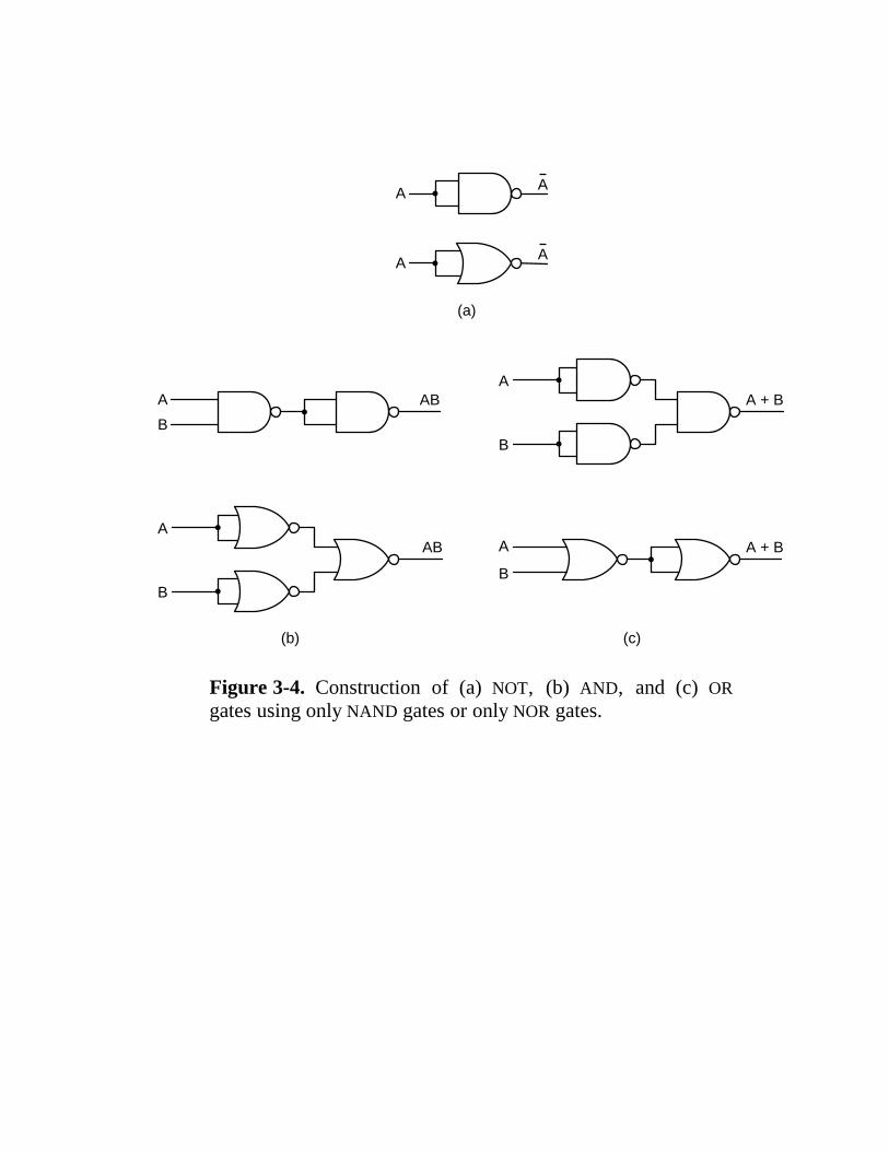
A + B
A + B
A
A
B
B
AB
AB
A
A
A
A
(a)
(b) (c)
A
B
A
B
Figure 3-4. Construction of (a) NOT, (b) AND, and (c) ORgates using only NAND gates or only NOR gates.

C
B
A A(B + C)
B + C
A
B
C
AB + AC
AB
AC
(a) (b)
A B C AB AC AB + AC
0 0 0 0 0 0
0 0 1 0 0 0
0 1 0 0 0 0
0 1 1 0 0 0
1 0 0 0 0 0
1 0 1 0 1 1
1 1 0 1 0 1
1 1 1 1 1 1
A B C A B + C A(B + C)
0 0 0 0 0 0
0 0 1 0 1 0
0 1 0 0 1 0
0 1 1 0 1 0
1 0 0 1 0 0
1 0 1 1 1 1
1 1 0 1 1 1
1 1 1 1 1 1
Figure 3-5. Two equivalent functions. (a) AB + AC. (b) A(B + C).
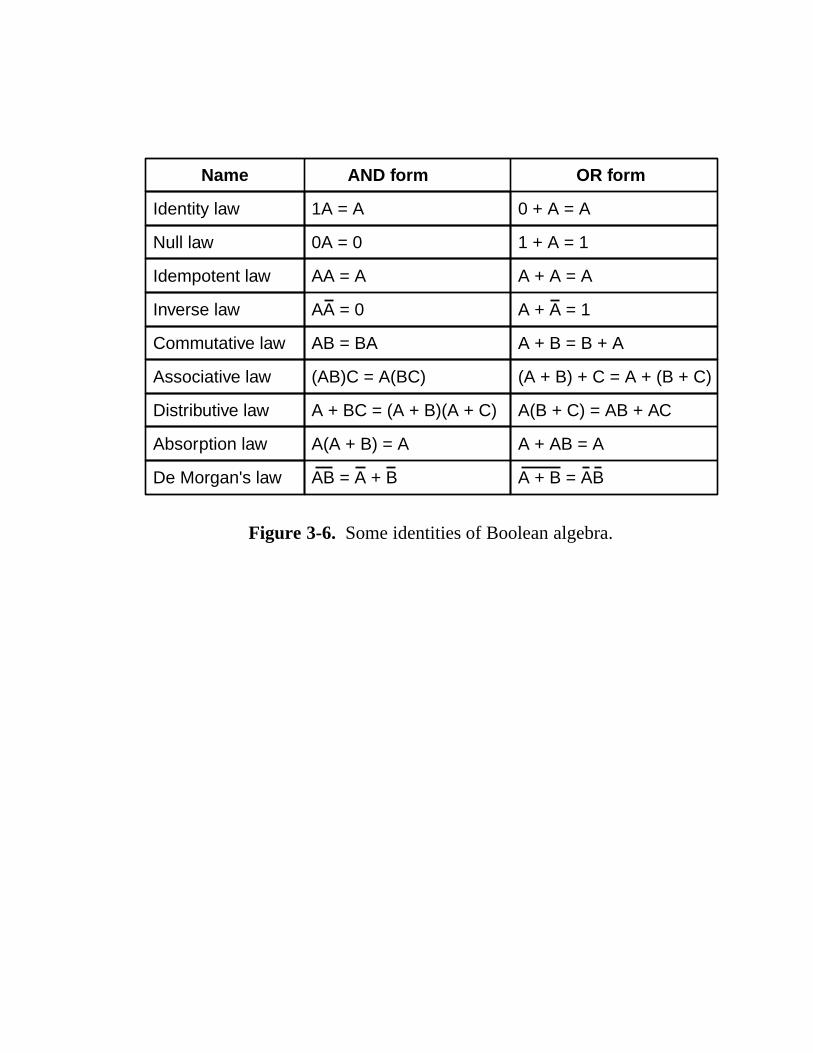
Identity law
Null law
Idempotent law
Inverse law
Commutative law
Associative law
Distributive law
Absorption law
De Morgan's law
1A = A
0A = 0
AA = A
AB = BA
(AB)C = A(BC)
A + BC = (A + B)(A + C)
A(A + B) = A A + AB = A
0 + A = A
1 + A = 1
A + A = A
A + B = B + A
(A + B) + C = A + (B + C)
A(B + C) = AB + AC
Name AND form OR form
AA = 0
AB = A + B
A + A = 1
A + B = AB
Figure 3-6. Some identities of Boolean algebra.
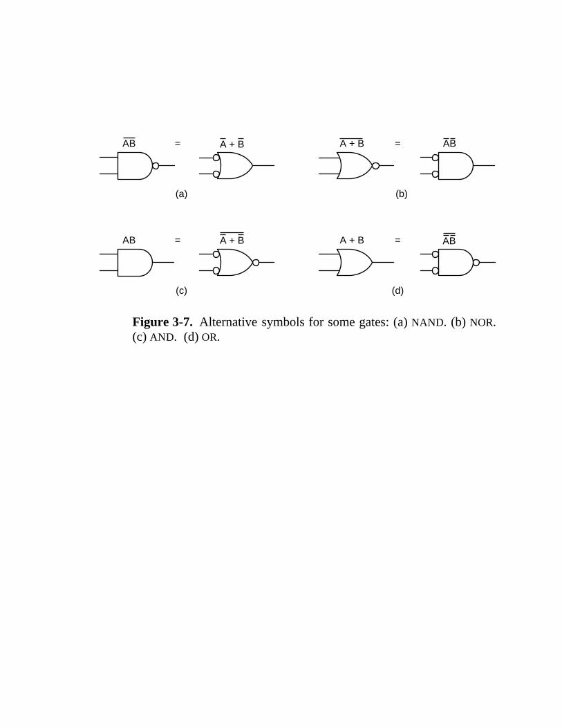
(a)
AB = A + B
(c)
A + BAB =
(b)
A + B = AB
AB=
(d)
A + B
Figure 3-7. Alternative symbols for some gates: (a) NAND. (b) NOR.(c) AND. (d) OR.

(a) (b)
A B XOR
0 0 0
0 1 1
1 0 1
1 1 0
A
B
B
A
(d)(c)
A
B
B
A
A
B
B
A
Figure 3-8. (a) The truth table for the XOR function. (b)-(d)Three circuits for computing it.

(a)
A B
0V 0V
0V 5V
5V 0V
5V 5V
F
0V
0V
0V
5V
(b)
A B
0 0
0 1
1 0
1 1
F
0
0
0
1
(c)
A B
1 1
1 0
0 1
0 0
F
1
1
1
0
Figure 3-9. (a) Electrical characteristics of a device.(b) Positive logic. (c) Negative logic.

Notch
11
VCC
Pin 8
GND
10 9 8121314
4 5 6 7321
Figure 3-10. An SSI chip containing four gates.

F
D0
D1
D2
D3
D4
D5
D6
D7
A B C
A A B CB C
Figure 3-11. An eight-input multiplexer circuit.

(a)
A B C
F
D0
D1
D2
D3
D4
D5
D6
D7
(b)
VCC
A B C
F
D0
D1
D2
D3
D4
D5
D6
D7
Figure 3-12. (a) An MSI multiplexer.. (b) The same multi-plexer wired to compute the majority function.

D0
D1
D2
D3
D4
D5
D6
D7
A
C
B
A
B
C
B
C
A
Figure 3-13. A 3-to-8 decoder circuit.

A = B
A0
B0
A1
B1
A2
B2
A3
B3
EXCLUSIVE OR gate
Figure 3-14. A simple 4-bit comparator.

A If this fuse isblown, B is notan input to ANDgate 1.
12 3 2 = 24input signals
24 input lines
6 outputs50 input
linesIf this fuse isblown, AND gate1 is not an inputto OR gate 5.
B
L
1 49
0
1
5
0
Figure 3-15. A 12-input, 6-output programmable logic array.The little squares represent fuses that can be burned out todetermine the function to be computed. The fuses are arrangedin two matrices: the upper one for the AND gates and the lowerone for the OR gates.

C
D0 D1 D2 D3 D4 D5 D6 D7
S0 S1 S2 S3 S4 S5 S6 S7
Figure 3-16. A 1-bit left/right shifter.

AA
B
B Sum
Sum
Carry
Carry
Exclusive OR gate
0 0 0 0
0 1 1 0
1 0 1 0
1 1 0 1
Figure 3-17. (a) Truth table for 1-bit addition. (b) A circuit for a half adder.

BA
B
Carryin Sum
SumCarryout
0 0 0 0
0 1 1 0
1 0 1 0
1
A
0
0
0
0 1 0 1
0 0 1 0
0 1 0 1
1 0 0 1
1
1
1
1
1 1 1 1
Carry in
Carry out
(a) (b)
Figure 3-18. (a) Truth table for full adder. (b) Circuit for a full adder.

AINVA
ENAB
Logical unit Carry in
AB
B
Enablelines
F0
F1
Decoder
Output
Sum
Carry out
Fulladder
A + B
ENB
Figure 3-19. A 1-bit ALU.
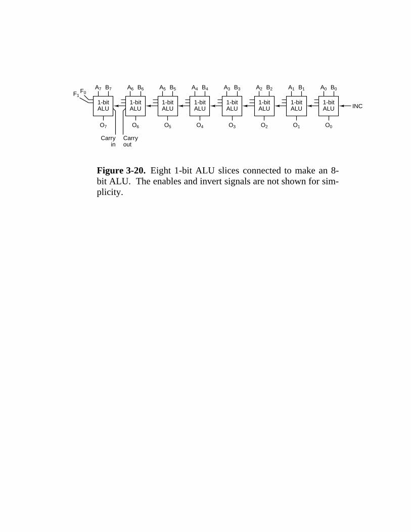
Carryin
Carryout
1-bitALU
F0F1
A7 B7
O7
1-bitALU
A6 B6
O6
1-bitALU
A5 B5
O5
1-bitALU
A4 B4
O4
1-bitALU
A3 B3
O3
1-bitALU
A2 B2
O2
1-bitALU
A1 B1
O1
1-bitALU INC
A0 B0
O0
Figure 3-20. Eight 1-bit ALU slices connected to make an 8-bit ALU. The enables and invert signals are not shown for sim-plicity.

Delay
C1
C2
(a) (b)
A
B
C
(c)
Figure 3-21. (a) A clock. (b) The timing diagram for theclock. (c) Generation of an asymmetric clock.

A B NOR
0 0 1
0 1 0
1 0 0
1 1 0
RQ
S0
0
1
00
1Q
RQ
S0
1
0
01
0Q
(a) (b) (c)
Figure 3-22. (a) NOR latch in state 0. (b) NOR latch in state 1.(c) Truth table for NOR.
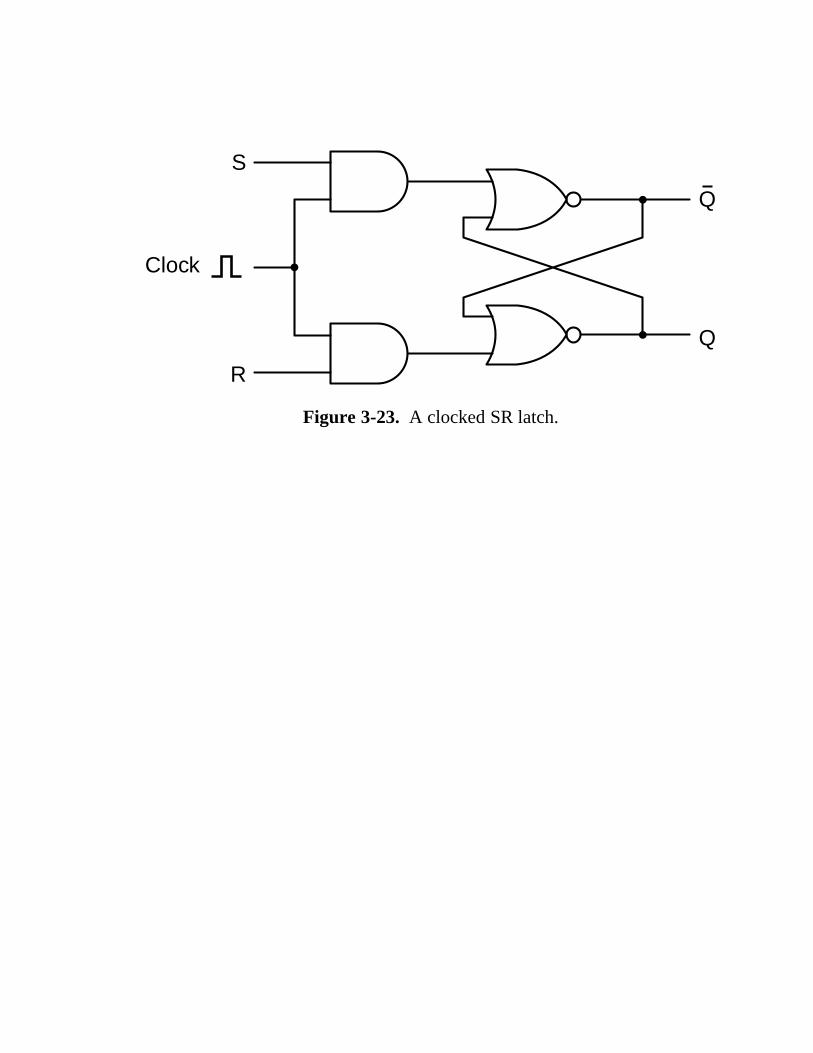
S
Q
Q
R
Clock
Figure 3-23. A clocked SR latch.

D
Q
Q
Figure 3-24. A clocked D latch.

a b
c
d
d
b AND c
Time
c
b
a
(a)
(b)
∆
Figure 3-25. (a) A pulse generator. (b) Timing at four points in the circuit.

Q
D
Q
Figure 3-26. A D flip-flop.
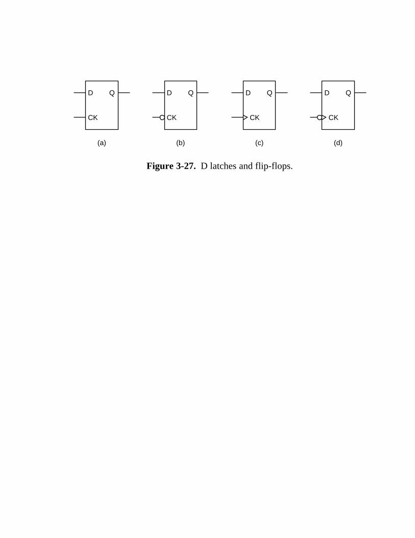
D Q
CK
(a)
D Q
CK
(b)
D Q
CK
(c)
D Q
(d)
CK
Figure 3-27. D latches and flip-flops.

D
14
Q
CK
CLR
PR
VCC
Q
D Q
CK
CLR
PRQ
13 12 11 10 9 8
1 2 3 4
(a)
5 6 7
GND
20
VCC
19 18 17 16 15 14 13 12 11
1 2 3 4 5 6 7 8 9 10
GND
(b)
Q D
CKCLR
D Q
CKCLR
Q D
CKCLR
D Q
CKCLR
Q D
CKCLR
Q D
CKCLR
Q D
CKCLR
Q D
CKCLR
Figure 3-28. (a) Dual D flip-flop. (b) Octal flip-flop.

Data in
Writegate
I0
I1
I2
QD
CKWord 0
Word 1
Word 2
Word 3
O1
O2
O3
CS
RD
OE
Word 0selectline
Word 1selectline
Word 2selectline
CS • RD
A0
A1
Output enable = CS • RD • OE
QD
CK
QD
CK
QD
CK
QD
CK
QD
CK
QD
CK
QD
CK
QD
CK
QD
CK
QD
CK
QD
CK
Figure 3-29. Logic diagram for a 4 × 3 memory. Each row isone of the four 3-bit words. A read or write operation alwaysreads or writes a complete word.

(b)(a)
Datain
Dataout
Control
(d)(c)
Figure 3-30. (a) A noninverting buffer. (b) Effect of (a) whencontrol is high. (c) Effect of (a) when control is low. (d) Aninverting buffer.

D0
A0A1A2A3A4A5A6A7A8A9
A10A11A12A13A14A15A16A17A18
D1D2D3D4D5D6D7
WE
(a)
512K 3 8Memory
chip
(4 Mbit)
CS OE
A0A1A2A3A4A5A6A7A8A9
A10
RAS
CAS
D
WE
(b)
4096K 3 1Memory
chip
(4 Mbit)
CS OE
Figure 3-31. Two ways of organizing a 4-Mbit memory chip.
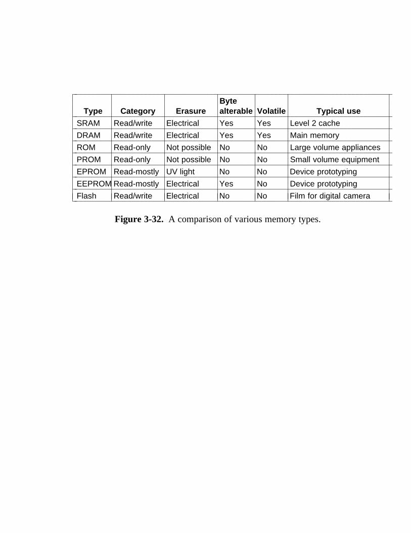
2222222222222222222222222222222222222222222222222222222222222222222222222222222
Type Category ErasureBytealterable Volatile Typical use2222222222222222222222222222222222222222222222222222222222222222222222222222222
SRAM Read/write Electrical Yes Yes Level 2 cache2222222222222222222222222222222222222222222222222222222222222222222222222222222DRAM Read/write Electrical Yes Yes Main memory2222222222222222222222222222222222222222222222222222222222222222222222222222222ROM Read-only Not possible No No Large volume appliances2222222222222222222222222222222222222222222222222222222222222222222222222222222PROM Read-only Not possible No No Small volume equipment2222222222222222222222222222222222222222222222222222222222222222222222222222222EPROM Read-mostly UV light No No Device prototyping2222222222222222222222222222222222222222222222222222222222222222222222222222222EEPROM Read-mostly Electrical Yes No Device prototyping2222222222222222222222222222222222222222222222222222222222222222222222222222222Flash Read/write Electrical No No Film for digital camera222222222222222222222222222222222222222222222222222222222222222222222222222222211111111111111
11111111111111
11111111111111
11111111111111
11111111111111
11111111111111
11111111111111
Figure 3-32. A comparison of various memory types.

TypicalMicro-
Processor
Symbol forelectrical ground
Symbolfor clock
signal
Bus arbitrationAddressing
Coprocessor
Status
MiscellaneousInterrupts
Bus control
Power is 5volts
+5v
Data
Φ
Figure 3-33. The logical pinout of a generic CPU. The arrowsindicate input signals and output signals. The short diagonallines indicate that multiple pins are used. For a specific CPU, anumber will be given to tell how many.

Buscontroller
Memory bus
I/O bus
DiskOn-chip bus
CPU chip
RegistersBuses
ALU
Memory
Modem Printer
Figure 3-34. A computer system with multiple buses.

222222222222222222222222222222222222222222222222222222222222222222222222222222Master Slave Example222222222222222222222222222222222222222222222222222222222222222222222222222222
CPU Memory Fetching instructions and data222222222222222222222222222222222222222222222222222222222222222222222222222222CPU I/O device Initiating data transfer222222222222222222222222222222222222222222222222222222222222222222222222222222CPU Coprocessor CPU handing instruction off to coprocessor222222222222222222222222222222222222222222222222222222222222222222222222222222I/O Memory DMA (Direct Memory Access)222222222222222222222222222222222222222222222222222222222222222222222222222222Coprocessor CPU Coprocessor fetching operands from CPU222222222222222222222222222222222222222222222222222222222222222222222222222222111111111
111111111
111111111
111111111
Figure 3-35. Examples of bus masters and slaves.

8088
(a)
20-Bit address
Control
80286
(b)
20-Bit address
4-Bit address
Control
4-Bit address
Control
Control
20-Bit address
Control
80386
(c)
8-Bit address
Control
Figure 3-36. Growth of an address bus over time.
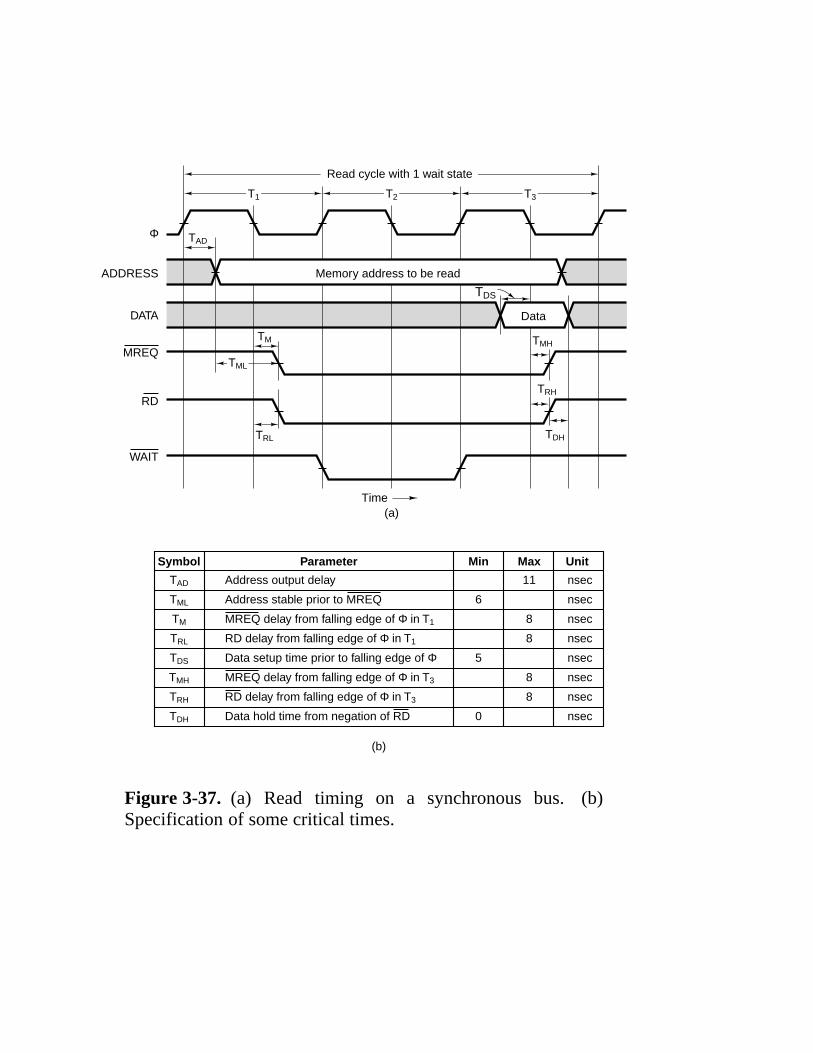
TAD
TML
TM
TRL
TDS
TMH
TRH
TDH
Address output delay
Address stable prior to MREQ
MREQ delay from falling edge of Φ in T1
RD delay from falling edge of Φ in T1
Data setup time prior to falling edge of Φ
MREQ delay from falling edge of Φ in T3
RD delay from falling edge of Φ in T3
Data hold time from negation of RD
6
5
0
(b)
11
8
8
8
8
nsec
nsec
nsec
nsec
nsec
nsec
nsec
nsec
ADDRESS
Time(a)
TAD
TM
TDS
TMH
TRH
TDHTRL
Φ
DATA
T1 T2 T3
MREQ
RD
WAIT
Read cycle with 1 wait state
Memory address to be read
Data
TML
Parameter Min Max UnitSymbol
Figure 3-37. (a) Read timing on a synchronous bus. (b)Specification of some critical times.
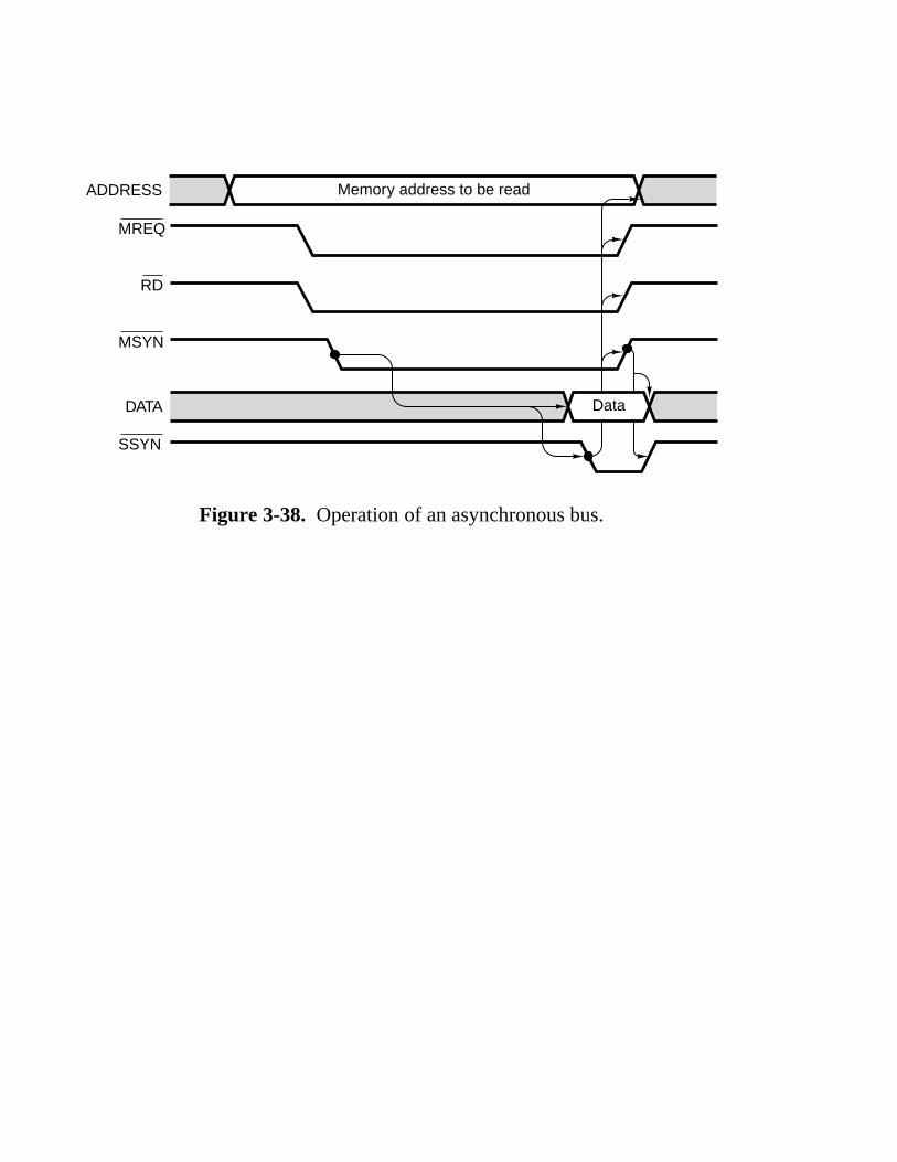
ADDRESS
MREQ
RD
MSYN
DATA
SSYN
Memory address to be read
Data
Figure 3-38. Operation of an asynchronous bus.

Bus grant
Bus request
I/O devices
(a)
(b)
Bus grantmay or may notbe propagated alongthe chain
Bus request level 1
Bus grant level 1
Bus request level 2Bus grant level 2
1 2 3 4 5
Arbiter
Arbiter
1 2 3 4 5
Figure 3-39. (a) A centralized one-level bus arbiter usingdaisy chaining. (b) The same arbiter, but with two levels.
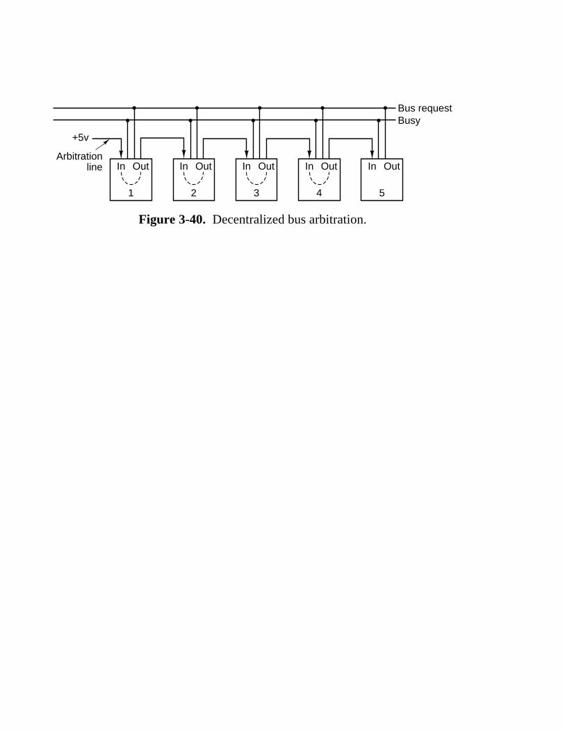
Arbitrationline
+5v
In Out
Bus requestBusy
1 2 3 4 5
In Out In Out In Out In Out
Figure 3-40. Decentralized bus arbitration.

Memory address to be read
Count
ADDRESS
Φ
DATA Data Data Data Data
T1 T2 T3 T4 T5 T6 T7
MREQ
RD
WAIT
BLOCK
Figure 3-41. A block transfer.

8259AInterruptcontroller
CPU
D0-D7
CSA0WR
INTA
RD
INT IR0IR1IR2IR3IR4IR5IR6IR7
+5 v
Keyboard
Clock
Disk
Printer
Figure 3-42. Use of the 8259A interrupt controller.
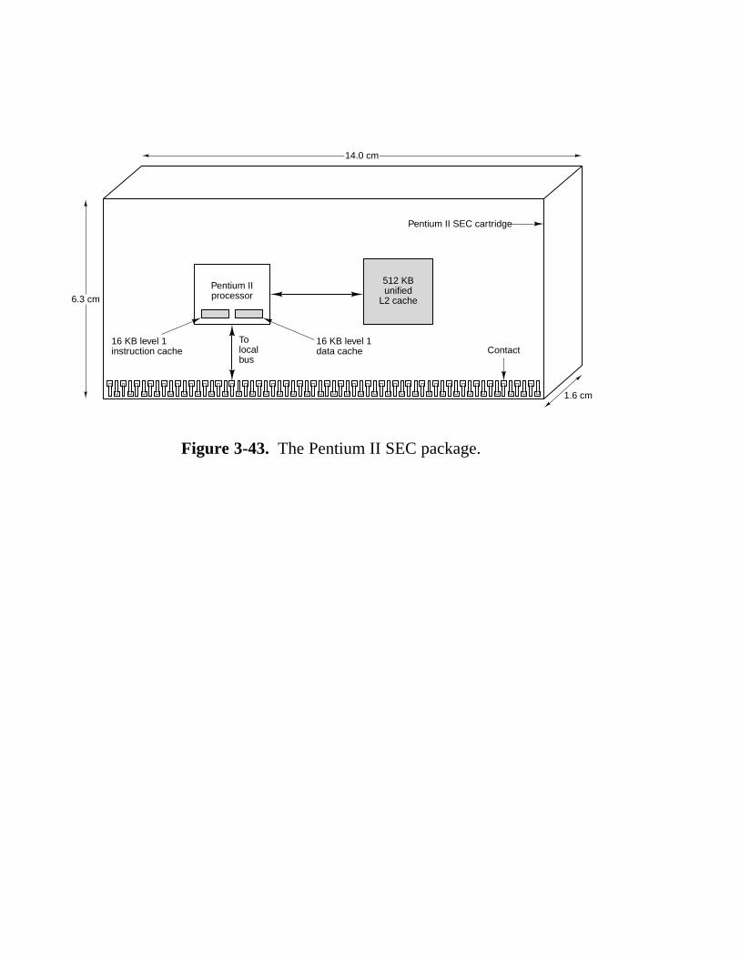
512 KBunified
L2 cache
Pentium IIprocessor
Contact
1.6 cm
16 KB level 1data cache
Tolocalbus
16 KB level 1instruction cache
Pentium II SEC cartridge
14.0 cm
6.3 cm
Figure 3-43. The Pentium II SEC package.

8
Parity#
7
35
2
3
11
4
RESET#
Interrupts
Compatibity
Diagnostics
Initialization
Power management
Miscellaneous
64
3
27
Power
5VID
TRDY#Response
RS#
3Misc#
5Misc#
Parity#
3
3
Parity#
5REQ#ADS#
33A#
Misc#
BPRI#
DBSY#DRDY#
LOCK#
D#
Pentium IICPU
Busarbitration
Request
Data
Snoop
Error
Φ
Figure 3-44. Logical pinout of the Pentium II. Names inupper case are the official Intel names for individual signals.Names in mixed case are groups of related signals or signaldescriptions.
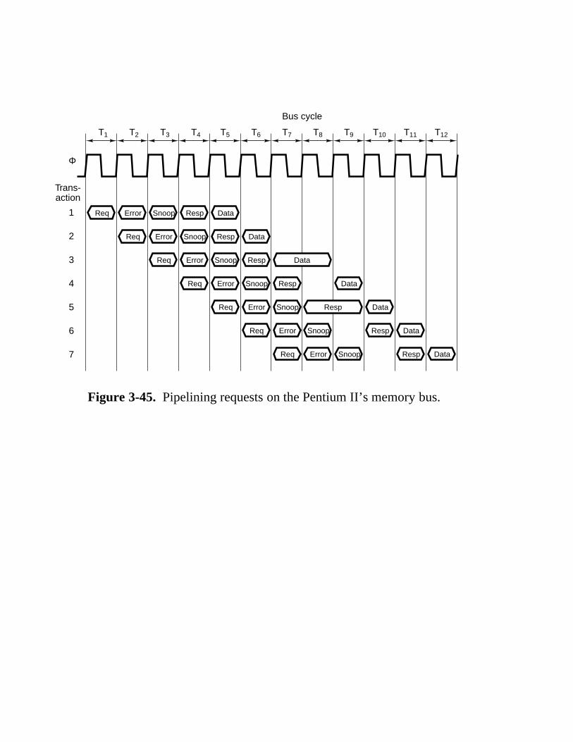
Trans-action
Φ
T1 T2 T3 T4 T5 T6
Req
T7
Bus cycle
1
2
3
4
5
6
7
T8 T9 T10 T11 T12
Error Snoop Resp Data
Req Error Snoop Resp Data
Req Error Snoop Resp Data
Resp
Req Error Snoop Resp Data
Req Error Snoop Data
Req Error Snoop Resp Data
Req Error Snoop Resp Data
Figure 3-45. Pipelining requests on the Pentium II’s memory bus.
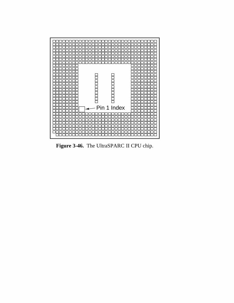
Pin 1 Index
Figure 3-46. The UltraSPARC II CPU chip.

Bus arbitration
Memory address
Address parity
Address valid
Wait
Reply
Level 1 caches
tomain
memory
UPAinterface
UltraSPARC IICPU
Tag address
Tag valid
Tag data
Tag parity
Level 2cachetags
Data address
Data address valid
Level 2cachedata
18 5
35
Memory data
Memory ECC
128
16
4
25
20
4
Data
Parity
128
16 5 Control
UDB IImemory
buffer
Figure 3-47. The main features of the core of an UltraSPARC II system.
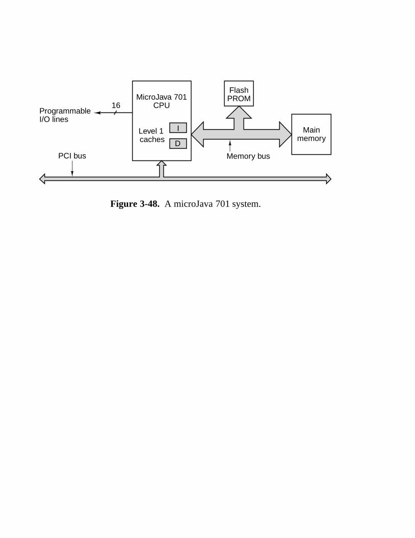
MicroJava 701CPU
Level 1 caches
PCI bus
ProgrammableI/O lines
FlashPROM
Mainmemory
Memory bus
16
I
D
Figure 3-48. A microJava 701 system.

Motherboard PC busPC bus
connector ContactPlug-inboard
Chips
CPU andotherchips
New connector for PC/AT Edge connector
Figure 3-49. The PC/AT bus has two components, the originalPC part and the new part.

ISAbridge
Modem
Mouse
PCIbridgeCPU
Mainmemory
SCSI USB
Local bus
Soundcard Printer Available
ISA slot
ISA bus
IDEdisk
AvailablePCI slot
Key-board
Mon-itor
Graphicsadaptor
Level 2cache
Cache bus Memory bus
PCI bus
Figure 3-50. Architecture of a typical Pentium II system. Thethicker buses have more bandwidth than the thinner ones.

PCIarbiter
PCIdevice
RE
Q#
GN
T#
PCIdevice
RE
Q#
GN
T#
PCIdevice
RE
Q#
GN
T#
PCIdevice
RE
Q#
GN
T#
Figure 3-51. The PCI bus uses a centralized bus arbiter.
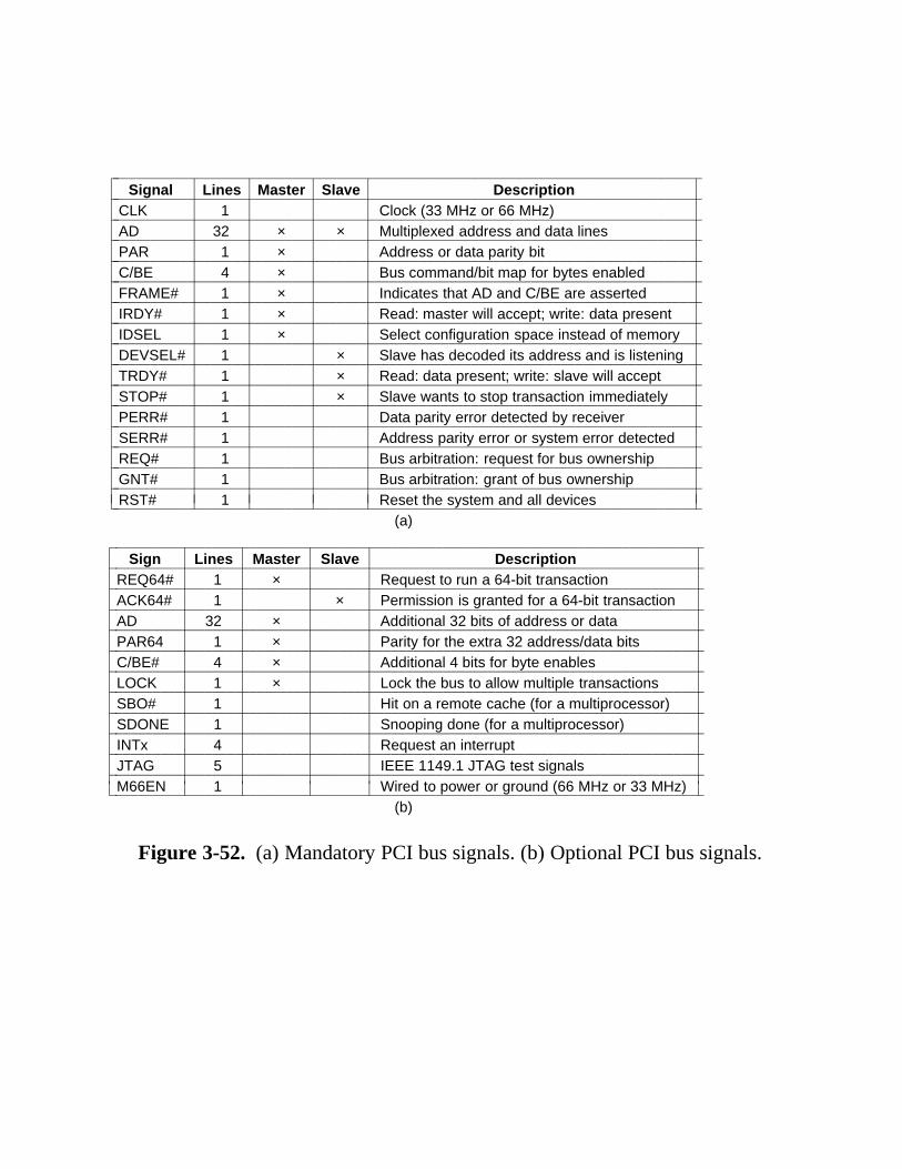
22222222222222222222222222222222222222222222222222222222222222222222222222222222Signal Lines Master Slave Description22222222222222222222222222222222222222222222222222222222222222222222222222222222
CLK 1 Clock (33 MHz or 66 MHz)22222222222222222222222222222222222222222222222222222222222222222222222222222222AD 32 × × Multiplexed address and data lines22222222222222222222222222222222222222222222222222222222222222222222222222222222PAR 1 × Address or data parity bit22222222222222222222222222222222222222222222222222222222222222222222222222222222C/BE 4 × Bus command/bit map for bytes enabled22222222222222222222222222222222222222222222222222222222222222222222222222222222FRAME# 1 × Indicates that AD and C/BE are asserted22222222222222222222222222222222222222222222222222222222222222222222222222222222IRDY# 1 × Read: master will accept; write: data present22222222222222222222222222222222222222222222222222222222222222222222222222222222IDSEL 1 × Select configuration space instead of memory22222222222222222222222222222222222222222222222222222222222222222222222222222222DEVSEL# 1 × Slave has decoded its address and is listening22222222222222222222222222222222222222222222222222222222222222222222222222222222TRDY# 1 × Read: data present; write: slave will accept22222222222222222222222222222222222222222222222222222222222222222222222222222222STOP# 1 × Slave wants to stop transaction immediately22222222222222222222222222222222222222222222222222222222222222222222222222222222PERR# 1 Data parity error detected by receiver22222222222222222222222222222222222222222222222222222222222222222222222222222222SERR# 1 Address parity error or system error detected22222222222222222222222222222222222222222222222222222222222222222222222222222222REQ# 1 Bus arbitration: request for bus ownership22222222222222222222222222222222222222222222222222222222222222222222222222222222GNT# 1 Bus arbitration: grant of bus ownership22222222222222222222222222222222222222222222222222222222222222222222222222222222RST# 1 Reset the system and all devices2222222222222222222222222222222222222222222222222222222222222222222222222222222211111111111111111111111
11111111111111111111111
11111111111111111111111
11111111111111111111111
11111111111111111111111
11111111111111111111111
(a)22222222222222222222222222222222222222222222222222222222222222222222222222222222
Sign Lines Master Slave Description22222222222222222222222222222222222222222222222222222222222222222222222222222222REQ64# 1 × Request to run a 64-bit transaction22222222222222222222222222222222222222222222222222222222222222222222222222222222ACK64# 1 × Permission is granted for a 64-bit transaction22222222222222222222222222222222222222222222222222222222222222222222222222222222AD 32 × Additional 32 bits of address or data22222222222222222222222222222222222222222222222222222222222222222222222222222222PAR64 1 × Parity for the extra 32 address/data bits22222222222222222222222222222222222222222222222222222222222222222222222222222222C/BE# 4 × Additional 4 bits for byte enables22222222222222222222222222222222222222222222222222222222222222222222222222222222LOCK 1 × Lock the bus to allow multiple transactions22222222222222222222222222222222222222222222222222222222222222222222222222222222SBO# 1 Hit on a remote cache (for a multiprocessor)22222222222222222222222222222222222222222222222222222222222222222222222222222222SDONE 1 Snooping done (for a multiprocessor)22222222222222222222222222222222222222222222222222222222222222222222222222222222INTx 4 Request an interrupt22222222222222222222222222222222222222222222222222222222222222222222222222222222JTAG 5 IEEE 1149.1 JTAG test signals22222222222222222222222222222222222222222222222222222222222222222222222222222222M66EN 1 Wired to power or ground (66 MHz or 33 MHz)2222222222222222222222222222222222222222222222222222222222222222222222222222222211111111111111111
11111111111111111
11111111111111111
11111111111111111
11111111111111111
11111111111111111
(b)
Figure 3-52. (a) Mandatory PCI bus signals. (b) Optional PCI bus signals.

Φ
T1 T2 T3 T4 T5 T6 T7
Turnaround
Address AddressData Data
Read Idle
Bus cycle
White
AD
C/BE#
FRAME#
IRDY#
DEVSEL#
TRDY#
Read cmd Write cmdEnable Enable
Figure 3-53. Examples of 32-bit PCI bus transactions. Thefirst three cycles are used for a read operation, then an idle cy-cle, and then three cycles for a write operation.

Time (msec)
0
Idle
Frame 0
Data packetfrom device
Packetsfrom root
Fromdevice
SOF
2
Frame 2
SOF
1
Frame 1
SOF IN DATA ACK
SYN PID PAYLOAD CRC
Packetsfrom root
3
Frame 3
SOF OUT DATA ACK
SYN PID PAYLOAD CRC
Figure 3-54. The USB root hub sends out frames every 1.00 msec.

CS
WR
RD
A0-A1
RESET
D0-D7
28
8
88
Port A
Port B
Port C
8255AParallel
I/Ochip
Figure 3-55. An 8255A PIO chip.

EPROM at address 0 RAM at address 8000H PIO at FFFCH
0 4K 8K 12K 16K 20K 24K 28K 32K 36K 40K 44K 48K 52K 56K 60K 64K
����� ���
�����
���
���
Figure 3-56. Location of the EPROM, RAM, and PIO in our 64K address space.

A0
A15
Address bus
A0
A15
Address bus
CS CS CS
2K 3 8EPROM
2K 3 8RAM PI0
(a)
(b)
CS CS CS
2K 3 8EPROM
2K 3 8RAM PI0
Figure 3-57. (a) Full address decoding. (b) Partial address decoding.

SEC. 3.5 181
3.6 EXAMPLE BUSES
Buses are the glue that hold computer systems together. In this section wewill take a close look at some popular buses: the ISA bus, the PCI bus, and theUniversal Serial Bus. The ISA bus is a slight expansion of the original IBM PCbus. For reasons of backward compatibility, it is still present in all Intel-basedPCs. However, these machines invariably have a second, faster bus as well: thePCI bus. The PCI bus is wider than the ISA bus and runs at a higher clock rate.The Universal serial bus is an increasingly popular I/O bus for low-speed peri-pherals such as mice and keyboards. In the following sections, we will look ateach of these buses in turn.
3.6.1 The ISA Bus
The IBM PC bus was the de facto standard on 8088-based systems becausenearly all PC clone vendors copied it in order to allow the many existing third-party I/O boards to be used with their systems. It had 62 signal lines, including 20for a memory address, 8 for data, and one each for asserting memory read,memory write, I/O read, and I/O write. There were also signals for requesting andgranting interrupts and using DMA, and that was about it. It was a very simplebus.
Physically, the bus was etched onto the PC’s motherboard, with about half adozen connectors spaced 2 cm apart into which cards could be inserted. Eachcard had a tab on it that fit in the connector. The tab had 31 gold-plated strips oneach side that made electrical contact with the connector.
When IBM introduced the 80286-based PC/AT, it had a major problem on itshands. If it had started from scratch and designed an entirely new 16-bit bus,many potential customers would have hesitated to buy it because none of the vastnumber of PC plug-in boards available from third-party vendors would haveworked using the new machine. On the other hand, sticking with the PC bus andits 20 address lines and 8 data lines would not have taken advantage of the80286’s ability to address 16M of memory and transfer 16-bit words.
The solution chosen was to extend the PC bus. PC plug-in cards have an edgeconnector with 62 contacts, but this edge connector does not run the full length ofthe board. The PC/AT solution was to put a second edge connector on the bottomof the board, adjacent to the main one, and design the AT circuitry to work withboth types of boards. The general idea is illustrated in Fig. 3-1.
The second connector on the PC/AT bus contains 36 lines. Of these, 31 areprovided for more address lines, more data lines, more interrupt lines, and moreDMA channels, as well as power and ground. The rest deal with differencesbetween 8-bit and 16-bit transfers.
When IBM brought out the PS/2 series as the successor to the PC and PC/AT,it decided that it was time to start again. Part of this decision may have been

182 THE DIGITAL LOGIC LEVEL CHAP. 3
Motherboard PC busPC bus
connector ContactPlug-inboard
Chips
CPU andotherchips
New connector for PC/AT Edge connector
Figure 3-1. The PC/AT bus has two components, the original PC part and the new part.
technical (the PC bus was by this time really obsolete), but part was no doubtcaused by a desire to put an obstacle in the way of companies making PC clones,which had taken over an uncomfortably large part of the market. Thus the mid-and upper-range PS/2 machines were equipped with a bus, the Microchannel, thatwas completely new, and which was protected by a wall of patents backed by anarmy of lawyers.
The rest of the personal computer industry reacted to this development byadopting its own standard, the ISA (Industry Standard Architecture) bus,which is basically the PC/AT bus running at 8.33 MHz. The advantage of thisapproach is that it retains compatibility with existing machines and cards. It alsois based on a bus that IBM had liberally licensed to many companies in order toensure that as many third parties as possible produced cards for the original PC,something that has come back to haunt IBM. Every Intel-based PC still has thisbus present, although usually with one or more other buses as well. A thoroughdescription of it can be found in (Shanley and Anderson, 1995a).
Later, the ISA bus was extended to 32 bits with a few new features thrown in(e.g., for multiprocessing). This new bus was called the EISA (Extended ISA)bus. Few boards have been produced for it, however.

SEC. 3.6 EXAMPLE BUSES 183
3.6.2 The PCI Bus
On the original IBM PC, most applications were text based. Gradually, withthe introduction of Windows, graphical user interfaces came into use. None ofthese applications put much of a strain on the ISA bus. However, as time went onand many applications, especially multimedia games, began to use computers todisplay full-screen, full-motion video, the situation changed radically.
Let us make a simple calculation. Consider a 1024 × 768 screen used for truecolor (3 bytes/pixel) moving images. One screen contains 2.25 MB of data. Forsmooth motion, at least 30 screens/sec are needed, for a data rate of 67.5 MB/sec.In fact, it is worse than this, since to display a video from a hard disk, CD-ROM,or DVD, the data must pass from the disk drive over the bus to the memory. Thenfor the display, the data must travel over the bus again to the graphics adapter.Thus we need a bus bandwidth of 135 MB/sec for the video alone, not countingthe bandwidth the CPU and other devices need.
The ISA bus runs at a maximum rate of 8.33 MHz, and can transfer 2 bytesper cycle, for a maximum bandwidth of 16.7 MB/sec. The EISA bus can move 4bytes per cycle, to achieve 33.3 MB/sec. Clearly, neither of these is even close towhat is needed for full-screen video.
In 1990, Intel saw this coming and designed a new bus with a much higherbandwidth than even the EISA bus. It was called the PCI bus (Peripheral Com-ponent Interconnect bus). To encourage its use, Intel patented the PCI bus andthen put all the patents into the public domain, so any company could build peri-pherals for it without having to pay royalties. Intel also formed an industry con-sortium, the PCI Special Interest Group, to manage the future of the PCI bus. Asa result of these actions, the PCI bus has become extremely popular. Virtuallyevery Intel-based computer since the Pentium has a PCI bus, and many othercomputers do, too. Sun even has a version of the UltraSPARC that uses the PCIbus, the UltraSPARC IIi. The PCI bus is covered in gory detail in (Shanley andAnderson, 1995b; and Solari and Willse, 1998).
The original PCI bus transferred 32 bits per cycle and ran at 33 MHz (30 nseccycle time) for a total bandwidth of 133 MB/sec. In 1993, PCI 2.0 was intro-duced, and in 1995, PCI 2.1 came out. PCI 2.2 has features for mobile computers(mostly for saving battery power). The PCI bus runs at up to 66 MHz and canhandle 64-bit transfers, for a total bandwidth of 528 MB/sec. With this kind ofcapacity, full-screen, full-motion video is doable (assuming the disk and the restof the system are up to the job). In any event, the PCI bus will not be thebottleneck.
Even though 528 MB/sec sounds pretty fast, it still has two problems. First, itis not good enough for a memory bus. Second, it is not compatible with all thoseold ISA cards out there. The solution Intel thought of was to design computerswith three or more buses, as shown in Fig. 3-2. Here we see that the CPU can talkto the main memory on a special memory bus, and that an ISA bus can be
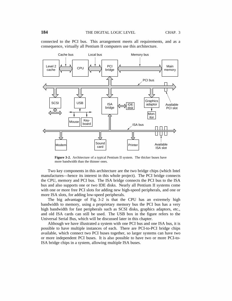
184 THE DIGITAL LOGIC LEVEL CHAP. 3
connected to the PCI bus. This arrangement meets all requirements, and as aconsequence, virtually all Pentium II computers use this architecture.
ISAbridge
Modem
Mouse
PCIbridgeCPU
Mainmemory
SCSI USB
Local bus
Soundcard Printer Available
ISA slot
ISA bus
IDEdisk
AvailablePCI slot
Key-board
Mon-itor
Graphicsadaptor
Level 2cache
Cache bus Memory bus
PCI bus
Figure 3-2. Architecture of a typical Pentium II system. The thicker buses havemore bandwidth than the thinner ones.
Two key components in this architecture are the two bridge chips (which Intelmanufactures—hence its interest in this whole project). The PCI bridge connectsthe CPU, memory and PCI bus. The ISA bridge connects the PCI bus to the ISAbus and also supports one or two IDE disks. Nearly all Pentium II systems comewith one or more free PCI slots for adding new high-speed peripherals, and one ormore ISA slots, for adding low-speed peripherals.
The big advantage of Fig. 3-2 is that the CPU has an extremely highbandwidth to memory, using a proprietary memory bus the PCI bus has a veryhigh bandwidth for fast peripherals such as SCSI disks, graphics adaptors, etc.,and old ISA cards can still be used. The USB box in the figure refers to theUniversal Serial Bus, which will be discussed later in this chapter.
Although we have illustrated a system with one PCI bus and one ISA bus, it ispossible to have multiple instances of each. There are PCI-to-PCI bridge chipsavailable, which connect two PCI buses together, so larger systems can have twoor more independent PCI buses. It is also possible to have two or more PCI-to-ISA bridge chips in a system, allowing multiple ISA buses.

SEC. 3.6 EXAMPLE BUSES 185
It would have been nice had there been one kind of PCI card. Unfortunately,such is not the case. Options are provided for voltage, width, and timing. Oldercomputers often use 5 volts and newer ones tend to use 3.3 volts, so the PCI bussupports both. The connectors are the same except for two bits of plastic that arethere to prevent people from inserting a 5-volt card in a 3.3-volt PCI bus or viceversa. Fortunately, universal cards, which support both voltages and can plug intoeither kind of slot, exist. In addition to the voltage option, cards come in 32-bitand 64-bit versions. The 32-bit cards have 120 pins; the 64-bit cards have thesame 120 pins plus an additional 64 pins, analogous to the way the IBM PC buswas extended to 16 bits (see Fig. 3-1). A PCI bus system that supports 64-bitcards can also take 32-bit cards, but the reverse is not true. Finally, PCI buses andcards can run at either 33 MHz or 66 MHz. The choice is made by having one pinwired either to the power supply or wired to ground. The connectors are identicalfor both speeds.
The PCI bus is synchronous, like all PC buses going back to the original IBMPC. All transactions on the PCI bus are between a master, officially called theinitiator, and a slave, officially called the target. To keep the PCI pin countdown, the address and data lines are multiplexed. In this way, only 64 pins areneeded on PCI cards for address plus data signals, even though PCI supports 64-bit addresses and 64-bit data.
The multiplexed address and data pins work as follows. On a read operation,during cycle 1, the master puts the address onto the bus. On cycle 2 the masterremoves the address and the bus is turned around so the slave can use it. On cycle3, the slave outputs the data requested. On write operations, the bus does not haveto be turned around because the master puts on both the address and the data.Nevertheless, the minimum transaction is still three cycles. If the slave is not ableto respond in three cycles, it can insert wait states. Block transfers of unlimitedsize are also allowed, as well as several other kinds of bus cycles.
PCI Bus Arbitration
To use the PCI bus, a device must first acquire it. PCI bus arbitration uses acentralized bus arbiter, as shown in Fig. 3-3. In most designs, the bus arbiter isbuilt into one of the bridge chips. Every PCI device has two dedicated lines run-ning from it to the arbiter. One line, REQ#, is used to request the bus. The otherline, GNT#, is used to receive bus grants.
To request the bus, a PCI device (including the CPU), asserts REQ# and waitsuntil it sees its GNT# line asserted by the arbiter. When that event happens, thedevice can use the bus on the next cycle. The algorithm used by the arbiter is notdefined by the PCI specification. Round robin arbitration, priority arbitration, andother schemes are all allowed. Clearly, a good arbiter will be fair, so as not to letsome devices wait forever.

186 THE DIGITAL LOGIC LEVEL CHAP. 3
PCIarbiter
PCIdevice
RE
Q#
GN
T#
PCIdevice
RE
Q#
GN
T#
PCIdevice
RE
Q#
GN
T#
PCIdevice
RE
Q#
GN
T#
Figure 3-3. The PCI bus uses a centralized bus arbiter.
A bus grant is for one transaction, although the length of this transaction istheoretically unbounded. If a device wants to run a second transaction and noother device is requesting the bus, it can go again, although normally one idlecycle between transactions has to be inserted. However, under special cir-cumstances, in the absence of competition for the bus, a device can make back-to-back transactions without having to insert an idle cycle. If a bus master is mak-ing a very long transfer and some other device has requested the bus, the arbitercan negate the GNT# line. The current bus master is expected to monitor the GNT#
line, so when it sees the negation, it must release the bus on the next cycle. Thisscheme allows very long transfers (which are efficient) when there is only onecandidate bus master but still gives fast response to competing devices.
PCI Bus Signals
The PCI bus has a number of mandatory signals, shown in Fig. 3-4(a), and anumber of optional signals, shown in Fig. 3-4(b). The remainder of the 120 or184 pins are used for power, ground, and related miscellaneous functions and arenot listed here. The Master (initiator) and Slave (target) columns tell who assertsthe signal on a normal transaction. If the signal is asserted by a different device(e.g., CLK), both columns are left blank.
Let us now look at each of the PCI bus signals briefly. We will start with themandatory (32-bit) signals; then we will move on to the optional (64-bit) signals.The CLK signal drives the bus. Most of the other signals are synchronous with it.In contrast to the ISA bus, a PCI bus transaction begins at the falling edge of CLK,which is in the middle of the cycle, rather than at the start.
The 32 AD signals are for the address and data (for 32-bit transactions). Gen-erally, during cycle 1 the address is asserted and during cycle 3 the data areasserted. The PAR signal is a parity bit for AD. The C/BE# signal is used for twodifferent things. On cycle 1, it contains the bus command (read 1 word, block

SEC. 3.6 EXAMPLE BUSES 187
22222222222222222222222222222222222222222222222222222222222222222222222222222222Signal Lines Master Slave Description22222222222222222222222222222222222222222222222222222222222222222222222222222222
CLK 1 Clock (33 MHz or 66 MHz)22222222222222222222222222222222222222222222222222222222222222222222222222222222AD 32 × × Multiplexed address and data lines22222222222222222222222222222222222222222222222222222222222222222222222222222222PAR 1 × Address or data parity bit22222222222222222222222222222222222222222222222222222222222222222222222222222222C/BE 4 × Bus command/bit map for bytes enabled22222222222222222222222222222222222222222222222222222222222222222222222222222222FRAME# 1 × Indicates that AD and C/BE are asserted22222222222222222222222222222222222222222222222222222222222222222222222222222222IRDY# 1 × Read: master will accept; write: data present22222222222222222222222222222222222222222222222222222222222222222222222222222222IDSEL 1 × Select configuration space instead of memory22222222222222222222222222222222222222222222222222222222222222222222222222222222DEVSEL# 1 × Slave has decoded its address and is listening22222222222222222222222222222222222222222222222222222222222222222222222222222222TRDY# 1 × Read: data present; write: slave will accept22222222222222222222222222222222222222222222222222222222222222222222222222222222STOP# 1 × Slave wants to stop transaction immediately22222222222222222222222222222222222222222222222222222222222222222222222222222222PERR# 1 Data parity error detected by receiver22222222222222222222222222222222222222222222222222222222222222222222222222222222SERR# 1 Address parity error or system error detected22222222222222222222222222222222222222222222222222222222222222222222222222222222REQ# 1 Bus arbitration: request for bus ownership22222222222222222222222222222222222222222222222222222222222222222222222222222222GNT# 1 Bus arbitration: grant of bus ownership22222222222222222222222222222222222222222222222222222222222222222222222222222222RST# 1 Reset the system and all devices2222222222222222222222222222222222222222222222222222222222222222222222222222222211111111111111111111111111
11111111111111111111111111
11111111111111111111111111
11111111111111111111111111
11111111111111111111111111
11111111111111111111111111
(a)
22222222222222222222222222222222222222222222222222222222222222222222222222222222Sign Lines Master Slave Description22222222222222222222222222222222222222222222222222222222222222222222222222222222
REQ64# 1 × Request to run a 64-bit transaction22222222222222222222222222222222222222222222222222222222222222222222222222222222ACK64# 1 × Permission is granted for a 64-bit transaction22222222222222222222222222222222222222222222222222222222222222222222222222222222AD 32 × Additional 32 bits of address or data22222222222222222222222222222222222222222222222222222222222222222222222222222222PAR64 1 × Parity for the extra 32 address/data bits22222222222222222222222222222222222222222222222222222222222222222222222222222222C/BE# 4 × Additional 4 bits for byte enables22222222222222222222222222222222222222222222222222222222222222222222222222222222LOCK 1 × Lock the bus to allow multiple transactions22222222222222222222222222222222222222222222222222222222222222222222222222222222SBO# 1 Hit on a remote cache (for a multiprocessor)22222222222222222222222222222222222222222222222222222222222222222222222222222222SDONE 1 Snooping done (for a multiprocessor)22222222222222222222222222222222222222222222222222222222222222222222222222222222INTx 4 Request an interrupt22222222222222222222222222222222222222222222222222222222222222222222222222222222JTAG 5 IEEE 1149.1 JTAG test signals22222222222222222222222222222222222222222222222222222222222222222222222222222222M66EN 1 Wired to power or ground (66 MHz or 33 MHz)222222222222222222222222222222222222222222222222222222222222222222222222222222221111111111111111111
1111111111111111111
1111111111111111111
1111111111111111111
1111111111111111111
1111111111111111111
(b)
Figure 3-4. (a) Mandatory PCI bus signals. (b) Optional PCI bus signals.
read, etc.). On cycle 2 it contains a bit map of 4 bits, telling which bytes of the32-bit word are valid. Using C/BE# it is possible to read or write any 1, 2, or 3bytes, as well as an entire word.
The FRAME# signal is asserted by the bus master to start a bus transaction. Ittells the slave that the address and bus commands are now valid. On a read,

188 THE DIGITAL LOGIC LEVEL CHAP. 3
usually IRDY# is asserted at the same time as FRAME#. It says the master is readyto accept the incoming data. On a write, IRDY# is asserted later, when the data areon the bus.
The IDSEL signal relates to the fact that every PCI device must have a 256-byte configuration space that other devices can read (by asserting IDSEL). Thisconfiguration space contains properties of the device. The Plug ’n Play feature ofsome operating systems uses the configuration space to find out what devices areon the bus.
Now we come to signals asserted by the slave. The first of these, DEVSEL#,announces that the slave has detected its address on the AD lines and is prepared toengage in the transaction. If DEVSEL# is not asserted within a certain time limit,the master times out and assumes the device addressed is either absent or broken.
The second slave signal is TRDY#, which the slave asserts on reads toannounce that the data are on the AD lines and on writes to announce that it isprepared to accept data.
The next three signals are for error reporting. The first of these is STOP#,which the slave asserts if something disastrous happens and it wants to abort thecurrent transaction. The next one, PERR#, is used to report a data parity error onthe previous cycle. For a read, it is asserted by the master; for a write it isasserted by the slave. It is up the the receiver to take the appropriate action.Finally, SERR# is for reporting address errors and system errors.
The REQ# and GNT# signals are for doing bus arbitration. These are notasserted by the current bus master, but rather by a device that wants to becomebus master. The last mandatory signal is RST#, used for resetting the system,either due to the user pushing the RESET button or some system device noticing afatal error. Asserting this signal resets all devices and reboots the computer.
Now we come to the optional signals, most of which relate to the expansionfrom 32 bits to 64 bits. The REQ64# and ACK64# signals allow the master to askpermission to conduct a 64-bit transaction and allow the slave to accept, respec-tively. The AD, PAR64, and C/BE# signals are just extensions of the corresponding32-bit signals.
The next three signals are not related to 32 bits versus 64 bits, but to multipro-cessor systems, something that PCI boards are not required to support. The LOCK
signal allows the bus to be locked for multiple transactions. The next two relateto bus snooping to maintain cache coherence.
The INTx signals are for requesting interrupts. A PCI card can have up to fourseparate logical devices on it, and each one can have its own interrupt requestline. The JTAG signals are for the IEEE 1149.1 JTAG testing procedure. Finally,the M66EN signal is either wired high or wired low, to set the clock speed. It mustnot change during system operation.
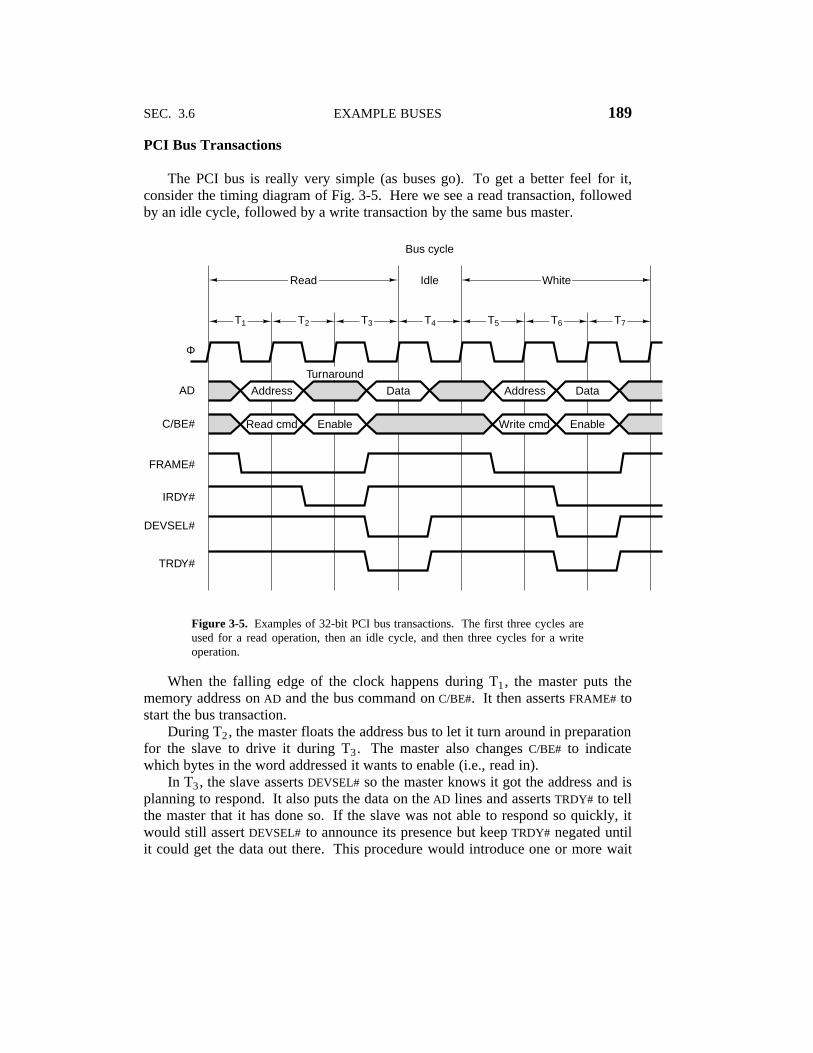
SEC. 3.6 EXAMPLE BUSES 189
PCI Bus Transactions
The PCI bus is really very simple (as buses go). To get a better feel for it,consider the timing diagram of Fig. 3-5. Here we see a read transaction, followedby an idle cycle, followed by a write transaction by the same bus master.
Φ
T1 T2 T3 T4 T5 T6 T7
Turnaround
Address AddressData Data
Read Idle
Bus cycle
White
AD
C/BE#
FRAME#
IRDY#
DEVSEL#
TRDY#
Read cmd Write cmdEnable Enable
Figure 3-5. Examples of 32-bit PCI bus transactions. The first three cycles areused for a read operation, then an idle cycle, and then three cycles for a writeoperation.
When the falling edge of the clock happens during T1, the master puts thememory address on AD and the bus command on C/BE#. It then asserts FRAME# tostart the bus transaction.
During T2, the master floats the address bus to let it turn around in preparationfor the slave to drive it during T3. The master also changes C/BE# to indicatewhich bytes in the word addressed it wants to enable (i.e., read in).
In T3, the slave asserts DEVSEL# so the master knows it got the address and isplanning to respond. It also puts the data on the AD lines and asserts TRDY# to tellthe master that it has done so. If the slave was not able to respond so quickly, itwould still assert DEVSEL# to announce its presence but keep TRDY# negated untilit could get the data out there. This procedure would introduce one or more wait

190 THE DIGITAL LOGIC LEVEL CHAP. 3
states.In this example (and often in reality), the next cycle is idle. Starting in T5 we
see the same master initiating a write. It starts out by putting the address andcommand onto the bus, as usual. Only now, in the second cycle it asserts the data.Since the same device is driving the AD lines, there is no need for a turnaroundcycle. In T7, the memory accepts the data.
3.6.3 The Universal Serial Bus
The PCI bus is fine for attaching high-speed peripherals to a computer, but itis far too expensive to have a PCI interface for each low-speed I/O device such asa keyboard or mouse. Historically, each standard I/O device was connected to thecomputer in a special way, with some free ISA and PCI slots for adding new dev-ices. Unfortunately, this scheme has been fraught with problems from the begin-ning. For example, each new I/O device often comes with its own ISA or PCIcard. The user is often responsible for setting switches and jumpers on the cardand making sure the settings do not conflict with other cards. Then the user mustopen up the case, carefully insert the card, close the case, and reboot the com-puter. For many users, this process is difficult and error prone. In addition, thenumber of ISA and PCI slots is very limited (two or three typically). Plug ’n Playcards eliminate the jumper settings, but the user still has to open the computer toinsert the card and bus slots are still limited.
To deal with this problem, in the mid 1990s, representatives from seven com-panies (Compaq, DEC, IBM, Intel, Microsoft, NEC, and Northern Telecom) gottogether to design a better way to attach low-speed I/O devices to a computer.Since then, hundreds of other companies have joined them. The resulting stan-dard is called USB (Universal Serial Bus) and it is being widely implemented inpersonal computers. It is described further in (Anderson, 1997; and Tan, 1997).
Some of the goals of the companies that originally conceived of the USB andstarted the project were as follows:
1. Users must not have to set switches or jumpers on boards or devices.
2. Users must not have to open the case to install new I/O devices.
3. There should be only one kind of cable, good for connecting all devices.
4. I/O devices should get their power from the cable.
5. Up to 127 devices should be attachable to a single computer.
6. The system should support real-time devices (e.g., sound, telephone).
7. Devices should be installable while the computer is running.
8. No reboot should be needed after installing a new device.
9. The new bus and its I/O devices should be inexpensive to manufacture.
SEC. 3.6 EXAMPLE BUSES 191
USB meets all these goals. It is designed for low-speed devices such as key-boards, mice, still cameras, snapshot scanners, digital telephones, and so on. Thetotal USB bandwidth is 1.5 MB/sec, which is enough for a substantial number ofthese devices. This low limit was chosen to keep the cost down.
A USB system consists of a root hub that plugs into the main bus (seeFig. 3-2). This hub has sockets for cables that can connect to I/O devices or toexpansion hubs, to provide more sockets, so the topology of a USB system is atree with its root at the root hub, inside the computer. The cables have differentconnectors on the hub end and on the device end, to prevent people from acciden-tally connecting two hub sockets together.
The cable consists of four wires: two for data, one for power (+5 volts), andone for ground. The signaling system transmits a 0 as a voltage transition and a 1as the absence of a voltage transition, so long runs of 0s generate a regular pulsestream.
When a new I/O device is plugged in, the root hub detects this event andinterrupts the operating system. The operating system then queries the device tofind out what it is and how much USB bandwidth it needs. If the operating sys-tem decides that there is enough bandwidth for the device, it assigns the new dev-ice a unique address (1 – 127) and downloads this address and other informationto configuration registers inside the device. In this way, new devices can beadded on-the-fly, without any user configuration required and without having toinstall new ISA or PCI cards. Uninitialized cards start out with address 0, so theycan be addressed. To make the cabling simpler, many USB devices containbuilt-in hubs to accept additional USB devices. For example, a monitor mighthave two hub sockets to accommodate the left and right speakers.
Logically, the USB system can be viewed as a set of bit pipes from the roothub to the I/O devices. Each device can split its bit pipe up into at most 16 sub-pipes for different types of data (e.g., audio and video). Within each pipe or sub-pipe, data flows from the root hub to the device or the other way. There is notraffic between two I/O devices.
Precisely every 1.00 ± 0.05 msec, the root hub broadcasts a new frame to keepall the devices synchronized in time. A frame is associated with a bit pipe, andconsists of packets, the first of which is from the root hub to the device. Subse-quent packets in the frame may also be in this direction, or they may be back fromthe device to the root hub. A sequence of four frames is shown in Fig. 3-6. InFig. 3-6 there is no work to be done in frames 0 and 2, so all that is needed is oneSOF (Start of Frame) packet. This packet is always broadcast to all devices.Frame 1 is a poll, for example, a request to a scanner to return the bits it has foundon the image it is scanning. Frame 3 consists of delivering data to some device,for example to a printer.
USB supports four kinds of frames: control, isochronous, bulk, and interrupt.Control frames are used to configure devices, give them commands, and inquireabout their status. Isochronous frames are for real-time devices such as

192 THE DIGITAL LOGIC LEVEL CHAP. 3
Time (msec)
0
Idle
Frame 0
Data packetfrom device
Packetsfrom root
Fromdevice
SOF
2
Frame 2
SOF
1
Frame 1
SOF IN DATA ACK
SYN PID PAYLOAD CRC
Packetsfrom root
3
Frame 3
SOF OUT DATA ACK
SYN PID PAYLOAD CRC
Figure 3-6. The USB root hub sounds out frames every 1.00 msec.
microphones, loudspeakers, and telephones that need to send or accept data at pre-cise time intervals. They have a highly-predictable delay but provide noretransmissions in the event of errors. Bulk frames are for large transfers to orfrom devices with no real-time requirements such as printers. Finally, interruptframes are needed because USB does not support interrupts. For example, insteadof having the keyboard cause an interrupt whenever a key is struck, the operatingsystem can poll it every 50 msec to collect any pending keystrokes.
A frame consists of one or more packets, possibly some in each direction.Four kinds of packets exist: token, data, handshake, and special. Token packetsare from the root to a device and are for system control. The SOF, IN, and OUT
packets in Fig. 3-6 are token packets. The SOF (Start of Frame) packet is the firstone in each frame and marks the beginning of the frame. If there is no work to do,the SOF packet is the only one in the frame. The IN token packet is a poll, askingthe device to return certain data. Fields in the IN packet tell which bit pipe isbeing polled so the device knows which data to return (if it has multiple streams).The OUT token packet announces that data for the device will follow. A fourthtype of token packet, SETUP (not shown in the figure), is used for configuration.
Besides the token packet, three other kinds exist. These are DATA (used totransmit up to 64 bytes of information either way), handshake, and special pack-ets. The format of a data packet is shown in Fig. 3-6. It consists of an 8-bit syn-chronization field, an 8-bit packet type (PID), the payload, and a 16-bit CRC(Cyclic Redundancy Code) to detect errors. Three kinds of handshake packetsare defined: ACK (the previous data packet was correctly received), NAK (a CRCerror was detected), and STALL (please wait—I am busy right now).
Now let us look at Fig. 3-6 again. Every 1.00 msec a frame must be sent fromthe root hub, even if there is no work. Frames 0 and 2 consist of just an SOF

SEC. 3.6 EXAMPLE BUSES 193
packet, indicating that there was no work. Frame 1 is a poll, so it starts out withSOF and IN packets from the computer to the I/O device, followed by a DATA
packet from the device to the computer. The ACK packet tells the device that thedata were received correctly. In case of an error, a NAK would be sent back to thedevice and the packet would be retransmitted for bulk data (but not for isochro-nous data). Frame 3 is similar in structure to frame 1, except that now the flow ofdata are from the computer to the device.

4THE MICROARCHITECTURE LEVEL
1

H
Shifter controlShifter
ALU
2
N
A B
B busC bus
6ALU control
Control signals
Memorycontrolregisters
Enable onto B bus
Write C bus to register
Toandfrommainmemory
Z
SP
LV
CPP
TOS
OPC
PC
MDR
MAR
MBR
Figure 4-1. The data path of the example microarchitecture used in this chapter.

2222222222222222222222222222222222222222222222222F0 F1 ENA ENB INVA INC Function22222222222222222222222222222222222222222222222220 1 1 0 0 0 A22222222222222222222222222222222222222222222222220 1 0 1 0 0 B22222222222222222222222222222222222222222222222220 1 1 0 1 0 A
332222222222222222222222222222222222222222222222222
1 0 1 1 0 0 B33
22222222222222222222222222222222222222222222222221 1 1 1 0 0 A + B22222222222222222222222222222222222222222222222221 1 1 1 0 1 A + B + 122222222222222222222222222222222222222222222222221 1 1 0 0 1 A + 122222222222222222222222222222222222222222222222221 1 0 1 0 1 B + 122222222222222222222222222222222222222222222222221 1 1 1 1 1 B − A22222222222222222222222222222222222222222222222221 1 0 1 1 1 B − 122222222222222222222222222222222222222222222222221 1 1 0 1 1 −A22222222222222222222222222222222222222222222222220 0 1 1 0 0 A AND B22222222222222222222222222222222222222222222222220 1 1 1 0 0 A OR B22222222222222222222222222222222222222222222222220 1 0 0 0 0 022222222222222222222222222222222222222222222222220 1 0 0 0 1 122222222222222222222222222222222222222222222222220 1 0 0 1 0 −1222222222222222222222222222222222222222222222222211
11111111111111111111111
1111111111111111111111111
1111111111111111111111111
1111111111111111111111111
1111111111111111111111111
1111111111111111111111111
1111111111111111111111111
1111111111111111111111111
Figure 4-2. Useful combinations of ALU signals and the function performed.

Cycle 1startshere
Shifteroutputstable
Registers loadedinstantaneously fromC bus and memory onrising edge of clock
Set upsignalsto drivedata path
ALUandshifter
Drive HandB bus
Propagationfrom shifterto registers
∆w ∆x ∆y ∆z
Clock cycle 1 Clock cycle 2
MPCavailablehere
New MPC used toload MIR with next microinstruction here
Figure 4-3. Timing diagram of one data path cycle.
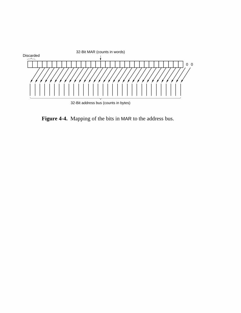
Discarded32-Bit MAR (counts in words)
32-Bit address bus (counts in bytes)
0 0
Figure 4-4. Mapping of the bits in MAR to the address bus.

Bits 9 3 8 9 3 4
NEXT_ADDRESS
Addr JAM ALU C Mem B
READ
FETCH
JAMN
JMPC
JAMZ
SLL8
SRA1
F0 F1 ENA
ENB
INVA
INC
H OPC
TOS
CPP
LV
SP
PC
MDR
MAR
WRITE
Bbus
B bus registers
0 = MDR1 = PC2 = MBR3 = MBRU4 = SP
5 = LV6 = CPP7 = TOS8 = OPC9 -15 none
Figure 4-5. The microinstruction format for the Mic-1.

H
Shifter
ALU
2
N
B bus
6
ALUcontrol
Controlsignals
Memory control signals (rd, wr, fetch)
EnableontoB bus
WriteC busto register
Z
C bus
SP
LV
CPP
TOS
OPC
PC
MDR
MAR
MBR
9
O
512 × 36-Bitcontrol storefor holding
the microprogram
3
8
4-to-16Decoder
2
8
4
MPC
MIRAddr J ALU C M B
1-bit flip–flop
Highbit
JMPC
JAMN/JAMZ
Figure 4-6. The complete block diagram of our example mi-croarchitecture, the Mic-1.

……
Address Addr Data path control bits
One ofthesewill follow0x75dependingon Z
JAM
JAMZ bit set0x75 0x92
0x92
0x192
001
Figure 4-7. A microinstruction with JAMZ set to 1 has two po-tential successors.

SP
LV
a3
a1
(a)
108
100a2 104
SP
LVa3
a1
(b)
a2
b3b4
b1b2
a3
a1
(c)
a2
b3b4
LV c1SP c2
b1b2
LVa3
a1
(d)
a2
d3d4
SP d5
d1d2
Figure 4-8. Use of a stack for storing local variables. (a)While A is active. (b) After A calls B. (c) After B calls C. (d)After C and B return and A calls D.

LV
a3
��������
SP a2
a1
(a)
a2LV
a3
��������
a2�����
SP a3
a1
(b)
a2LV
a3
��������
SP a2 + a3
a1
(c)
a2LV
SP a3
a2 + a3
(d)
a2
Figure 4-9. Use of an operand stack for doing an arithmetic computation.

SP
LV
PC
CPP
ConstantPool
CurrentOperandStack 3
CurrentLocal
VariableFrame 3
LocalVariableFrame 2
LocalVariableFrame 1
MethodArea
Figure 4-10. The various parts of the IJVM memory.

222222222222222222222222222222222222222222222222222222222222222222222222222222222Hex Mnemonic Meaning2222222222222222222222222222222222222222222222222222222222222222222222222222222220x10 BIPUSH byte Push byte onto stack2222222222222222222222222222222222222222222222222222222222222222222222222222222220x59 DUP Copy top word on stack and push onto stack2222222222222222222222222222222222222222222222222222222222222222222222222222222220xA7 GOTO offset Unconditional branch2222222222222222222222222222222222222222222222222222222222222222222222222222222220x60 IADD Pop two words from stack; push their sum2222222222222222222222222222222222222222222222222222222222222222222222222222222220x7E IAND Pop two words from stack; push Boolean AND2222222222222222222222222222222222222222222222222222222222222222222222222222222220x99 IFEQ offset Pop word from stack and branch if it is zero2222222222222222222222222222222222222222222222222222222222222222222222222222222220x9B IFLT offset Pop word from stack and branch if it is less than zero2222222222222222222222222222222222222222222222222222222222222222222222222222222220x9F IF3ICMPEQ offset Pop two words from stack; branch if equal2222222222222222222222222222222222222222222222222222222222222222222222222222222220x84 IINC varnum const Add a constant to a local variable2222222222222222222222222222222222222222222222222222222222222222222222222222222220x15 ILOAD varnum Push local variable onto stack2222222222222222222222222222222222222222222222222222222222222222222222222222222220xB6 INVOKEVIRTUAL disp Invoke a method2222222222222222222222222222222222222222222222222222222222222222222222222222222220x80 IOR Pop two words from stack; push Boolean OR2222222222222222222222222222222222222222222222222222222222222222222222222222222220xAC IRETURN Return from method with integer value2222222222222222222222222222222222222222222222222222222222222222222222222222222220x36 ISTORE varnum Pop word from stack and store in local variable2222222222222222222222222222222222222222222222222222222222222222222222222222222220x64 ISUB Pop two words from stack; push their difference2222222222222222222222222222222222222222222222222222222222222222222222222222222220x13 LDC3W index Push constant from constant pool onto stack2222222222222222222222222222222222222222222222222222222222222222222222222222222220x00 NOP Do nothing2222222222222222222222222222222222222222222222222222222222222222222222222222222220x57 POP Delete word on top of stack2222222222222222222222222222222222222222222222222222222222222222222222222222222220x5F SWAP Swap the two top words on the stack2222222222222222222222222222222222222222222222222222222222222222222222222222222220xC4 WIDE Prefix instruction; next instruction has a 16-bit index2222222222222222222222222222222222222222222222222222222222222222222222222222222221111111111111111111111111111111
1111111111111111111111111111111
1111111111111111111111111111111
1111111111111111111111111111111
Figure 4-11. The IJVM instruction set. The operands byte,const, and varnum are 1 byte. The operands disp, index, andoffset are 2 bytes.
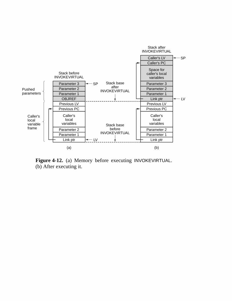
Pushedparameters
Caller'slocalvariableframe
Stack beforeINVOKEVIRTUAL
Stack afterINVOKEVIRTUAL
SP
SP
LV
LV
(a) (b)
Stack baseafter
INVOKEVIRTUAL
Stack basebefore
INVOKEVIRTUAL
Parameter 3Parameter 2Parameter 1
OBJREFPrevious LVPrevious PC Previous PC
Caller'slocal
variables
Parameter 2Parameter 1
Link ptr
Caller'slocal
variables
Space forcaller's local
variables
Parameter 2Parameter 1
Link ptr
Caller's LVCaller's PC
Previous LV
Parameter 3Parameter 2Parameter 1
Link ptr
Figure 4-12. (a) Memory before executing INVOKEVIRTUAL.(b) After executing it.

Caller'slocalvariableframe
Stack beforeIRETURN
Stack afterIRETURN
SP
SPLV
LV
(a) (b)
Stack basebefore
IRETURN
Stack baseafter
IRETURN
Parameter 3Parameter 2Parameter 1
Link ptrPrevious LVPrevious PC Previous PC
Caller'slocal
variables
Caller'slocal
variables
Parameter 2Parameter 1
Previous LVReturn value
Previous PC
Link ptr
Caller'slocal
variables
Parameter 2Parameter 1
Link ptr
Previous LVReturn value
Figure 4-13. (a) Memory before executing IRETURN. (b) After executing it.

i = j + k; 1 ILOAD j // i = j + k 0x15 0x02if (i == 3) 2 ILOAD k 0x15 0x03
k = 0; 3 IADD 0x60else 4 ISTORE i 0x36 0x01
j = j − 1; 5 ILOAD i // if (i < 3) 0x15 0x016 BIPUSH 3 0x10 0x037 IF3ICMPEQ L1 0x9F 0x00 0x0D8 ILOAD j // j = j − 1 0x15 0x029 BIPUSH 1 0x10 0x01
10 ISUB 0x6411 ISTORE j 0x36 0x0212 GOTO L2 0xA7 0x00 0x0713 L1: BIPUSH 0 // k = 0 0x10 0x0014 ISTORE k 0x36 0x0315 L2:
(a) (b) (c)
Figure 4-14. (a) A Java fragment. (b) The corresponding Javaassembly language. (c) The IJVM program in hexadecimal.

j2
j + k3
j10
kj6 7
3
4j5
j – 110 11
j1
j98 14 1512
013
Figure 4-15. The stack after each instruction of Fig. 4-14(b).

222222222222222222222222222DEST = H222222222222222222222222222DEST = SOURCE222222222222222222222222222DEST = H
33222222222222222222222222222DEST = SOURCE
333333333222222222222222222222222222DEST = H + SOURCE222222222222222222222222222DEST = H + SOURCE + 1222222222222222222222222222DEST = H + 1222222222222222222222222222DEST = SOURCE + 1222222222222222222222222222DEST = SOURCE − H222222222222222222222222222DEST = SOURCE − 1222222222222222222222222222DEST = −H222222222222222222222222222DEST = H AND SOURCE222222222222222222222222222DEST = H OR SOURCE222222222222222222222222222DEST = 0222222222222222222222222222DEST = 1222222222222222222222222222DEST = −122222222222222222222222222211111111111111111111111
11111111111111111111111
Figure 4-16. All permitted operations. Any of the aboveoperations may be extended by adding ‘‘<< 8’’ to them to shiftthe result left by 1 byte. For example, a common operation isH = MBR < < 8
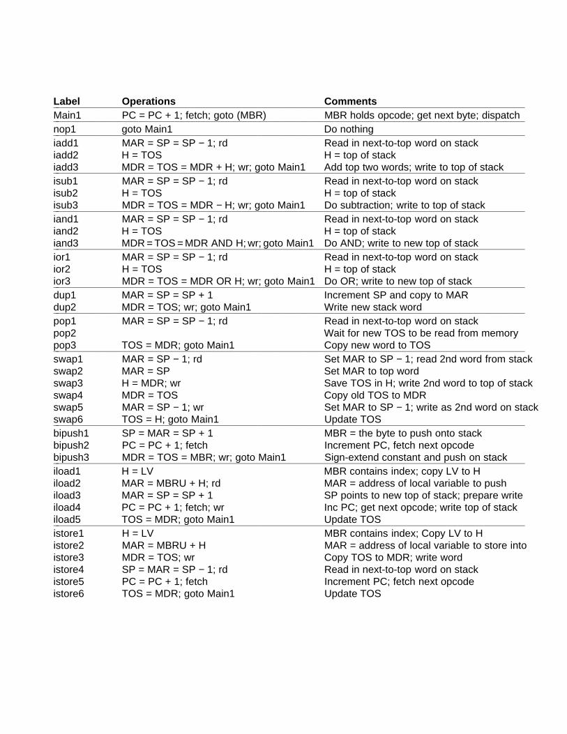
Label Operations Comments22222222222222222222222222222222222222222222222222222222222222222222222222222222222222222222Main1 PC = PC + 1; fetch; goto (MBR) MBR holds opcode; get next byte; dispatch22222222222222222222222222222222222222222222222222222222222222222222222222222222222222222222nop1 goto Main1 Do nothing22222222222222222222222222222222222222222222222222222222222222222222222222222222222222222222iadd1 MAR = SP = SP − 1; rd Read in next-to-top word on stackiadd2 H = TOS H = top of stackiadd3 MDR = TOS = MDR + H; wr; goto Main1 Add top two words; write to top of stack22222222222222222222222222222222222222222222222222222222222222222222222222222222222222222222isub1 MAR = SP = SP − 1; rd Read in next-to-top word on stackisub2 H = TOS H = top of stackisub3 MDR = TOS = MDR − H; wr; goto Main1 Do subtraction; write to top of stack22222222222222222222222222222222222222222222222222222222222222222222222222222222222222222222iand1 MAR = SP = SP − 1; rd Read in next-to-top word on stackiand2 H = TOS H = top of stackiand3 MDR = TOS = MDR AND H; wr; goto Main1 Do AND; write to new top of stack22222222222222222222222222222222222222222222222222222222222222222222222222222222222222222222ior1 MAR = SP = SP − 1; rd Read in next-to-top word on stackior2 H = TOS H = top of stackior3 MDR = TOS = MDR OR H; wr; goto Main1 Do OR; write to new top of stack22222222222222222222222222222222222222222222222222222222222222222222222222222222222222222222dup1 MAR = SP = SP + 1 Increment SP and copy to MARdup2 MDR = TOS; wr; goto Main1 Write new stack word22222222222222222222222222222222222222222222222222222222222222222222222222222222222222222222pop1 MAR = SP = SP − 1; rd Read in next-to-top word on stackpop2 Wait for new TOS to be read from memorypop3 TOS = MDR; goto Main1 Copy new word to TOS22222222222222222222222222222222222222222222222222222222222222222222222222222222222222222222swap1 MAR = SP − 1; rd Set MAR to SP − 1; read 2nd word from stackswap2 MAR = SP Set MAR to top wordswap3 H = MDR; wr Save TOS in H; write 2nd word to top of stackswap4 MDR = TOS Copy old TOS to MDRswap5 MAR = SP − 1; wr Set MAR to SP − 1; write as 2nd word on stackswap6 TOS = H; goto Main1 Update TOS22222222222222222222222222222222222222222222222222222222222222222222222222222222222222222222bipush1 SP = MAR = SP + 1 MBR = the byte to push onto stackbipush2 PC = PC + 1; fetch Increment PC, fetch next opcodebipush3 MDR = TOS = MBR; wr; goto Main1 Sign-extend constant and push on stack22222222222222222222222222222222222222222222222222222222222222222222222222222222222222222222iload1 H = LV MBR contains index; copy LV to Hiload2 MAR = MBRU + H; rd MAR = address of local variable to pushiload3 MAR = SP = SP + 1 SP points to new top of stack; prepare writeiload4 PC = PC + 1; fetch; wr Inc PC; get next opcode; write top of stackiload5 TOS = MDR; goto Main1 Update TOS22222222222222222222222222222222222222222222222222222222222222222222222222222222222222222222istore1 H = LV MBR contains index; Copy LV to Histore2 MAR = MBRU + H MAR = address of local variable to store intoistore3 MDR = TOS; wr Copy TOS to MDR; write wordistore4 SP = MAR = SP − 1; rd Read in next-to-top word on stackistore5 PC = PC + 1; fetch Increment PC; fetch next opcodeistore6 TOS = MDR; goto Main1 Update TOS

22222222222222222222222222222222222222222222222222222222222222222222222222222222222222222222wide1 PC = PC + 1; fetch; goto (MBR OR 0x100) Multiway branch with high bit set22222222222222222222222222222222222222222222222222222222222222222222222222222222222222222222wide3iload1 PC = PC + 1; fetch MBR contains 1st index byte; fetch 2ndwide3iload2 H = MBRU << 8 H = 1st index byte shifted left 8 bitswide3iload3 H = MBRU OR H H = 16-bit index of local variablewide3iload4 MAR = LV + H; rd; goto iload3 MAR = address of local variable to push22222222222222222222222222222222222222222222222222222222222222222222222222222222222222222222wide3istore1 PC = PC + 1; fetch MBR contains 1st index byte; fetch 2ndwide3istore2 H = MBRU << 8 H = 1st index byte shifted left 8 bitswide3istore3 H = MBRU OR H H = 16-bit index of local variablewide3istore4 MAR = LV + H; goto istore3 MAR = address of local variable to store into22222222222222222222222222222222222222222222222222222222222222222222222222222222222222222222ldc3w1 PC = PC + 1; fetch MBR contains 1st index byte; fetch 2ndldc3w2 H = MBRU << 8 H = 1st index byte << 8ldc3w3 H = MBRU OR H H = 16-bit index into constant poolldc3w4 MAR = H + CPP; rd; goto iload3 MAR = address of constant in pool
Figure 4-17. The microprogram for the Mic-1 (part 1 of 3).

Label Operations Comments222222222222222222222222222222222222222222222222222222222222222222222222222222222222222iinc1 H = LV MBR contains index; Copy LV to Hiinc2 MAR = MBRU + H; rd Copy LV + index to MAR; Read variableiinc3 PC = PC + 1; fetch Fetch constantiinc4 H = MDR Copy variable to Hiinc5 PC = PC + 1; fetch Fetch next opcodeiinc6 MDR = MBR + H; wr; goto Main1 Put sum in MDR; update variable222222222222222222222222222222222222222222222222222222222222222222222222222222222222222goto1 OPC = PC − 1 Save address of opcode.goto2 PC = PC + 1; fetch MBR = 1st byte of offset; fetch 2nd bytegoto3 H = MBR << 8 Shift and save signed first byte in Hgoto4 H = MBRU OR H H = 16-bit branch offsetgoto5 PC = OPC + H; fetch Add offset to OPCgoto6 goto Main1 Wait for fetch of next opcode222222222222222222222222222222222222222222222222222222222222222222222222222222222222222iflt1 MAR = SP = SP − 1; rd Read in next-to-top word on stackiflt2 OPC = TOS Save TOS in OPC temporarilyiflt3 TOS = MDR Put new top of stack in TOSiflt4 N = OPC; if (N) goto T; else goto F Branch on N bit222222222222222222222222222222222222222222222222222222222222222222222222222222222222222ifeq1 MAR = SP = SP − 1; rd Read in next-to-top word of stackifeq2 OPC = TOS Save TOS in OPC temporarilyifeq3 TOS = MDR Put new top of stack in TOSifeq4 Z = OPC; if (Z) goto T; else goto F Branch on Z bit222222222222222222222222222222222222222222222222222222222222222222222222222222222222222if3icmpeq1 MAR = SP = SP − 1; rd Read in next-to-top word of stackif3icmpeq2 MAR = SP = SP − 1 Set MAR to read in new top-of-stackif3icmpeq3 H = MDR; rd Copy second stack word to Hif3icmpeq4 OPC = TOS Save TOS in OPC temporarilyif3icmpeq5 TOS = MDR Put new top of stack in TOSif3icmpeq6 Z = OPC − H; if (Z) goto T; else goto F If top 2 words are equal, goto T, else goto F222222222222222222222222222222222222222222222222222222222222222222222222222222222222222T OPC = PC − 1; fetch; goto goto2 Same as goto1; needed for target address222222222222222222222222222222222222222222222222222222222222222222222222222222222222222F PC = PC + 1 Skip first offset byteF2 PC = PC + 1; fetch PC now points to next opcodeF3 goto Main1 Wait for fetch of opcode

222222222222222222222222222222222222222222222222222222222222222222222222222222222222222invokevirtual1 PC = PC + 1; fetch MBR = index byte 1; inc. PC, get 2nd byteinvokevirtual2 H = MBRU << 8 Shift and save first byte in Hinvokevirtual3 H = MBRU OR H H = offset of method pointer from CPPinvokevirtual4 MAR = CPP + H; rd Get pointer to method from CPP areainvokevirtual5 OPC = PC + 1 Save Return PC in OPC temporarilyinvokevirtual6 PC = MDR; fetch PC points to new method; get param countinvokevirtual7 PC = PC + 1; fetch Fetch 2nd byte of parameter countinvokevirtual8 H = MBRU << 8 Shift and save first byte in Hinvokevirtual9 H = MBRU OR H H = number of parametersinvokevirtual10 PC = PC + 1; fetch Fetch first byte of # localsinvokevirtual11 TOS = SP − H TOS = address of OBJREF − 1invokevirtual12 TOS = MAR = TOS + 1 TOS = address of OBJREF (new LV)invokevirtual13 PC = PC + 1; fetch Fetch second byte of # localsinvokevirtual14 H = MBRU << 8 Shift and save first byte in Hinvokevirtual15 H = MBRU OR H H = # localsinvokevirtual16 MDR = SP + H + 1; wr Overwrite OBJREF with link pointerinvokevirtual17 MAR = SP = MDR; Set SP, MAR to location to hold old PCinvokevirtual18 MDR = OPC; wr Save old PC above the local variablesinvokevirtual19 MAR = SP = SP + 1 SP points to location to hold old LVinvokevirtual20 MDR = LV; wr Save old LV above saved PCinvokevirtual21 PC = PC + 1; fetch Fetch first opcode of new method.invokevirtual22 LV = TOS; goto Main1 Set LV to point to LV Frame
Figure 4-17. The microprogram for the Mic-1 (part 2 of 3).

Label Operations Comments2222222222222222222222222222222222222222222222222222222222222222222222ireturn1 MAR = SP = LV; rd Reset SP, MAR to get link pointerireturn2 Wait for readireturn3 LV = MAR = MDR; rd Set LV to link ptr; get old PCireturn4 MAR = LV + 1 Set MAR to read old LVireturn5 PC = MDR; rd; fetch Restore PC; fetch next opcodeireturn6 MAR = SP Set MAR to write TOSireturn7 LV = MDR Restore LVireturn8 MDR = TOS; wr; goto Main1 Save return value on original top of stack
Figure 4-17. The microprogram for the Mic-1 (part 3 of 3).

BYTEBIPUSH(0×10)
Figure 4-18. The BIPUSH instruction format.
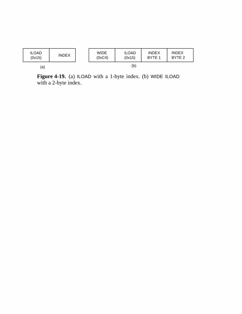
INDEXBYTE 1
INDEXBYTE 2
WIDE(0xC4)
ILOAD(0x15)
ILOAD(0x15)
INDEX
(a) (b)
Figure 4-19. (a) ILOAD with a 1-byte index. (b) WIDE ILOADwith a 2-byte index.

Address Control store
Microinstructionexecution order
ILOADWIDEILOAD
wide_iload1
Main1 1
wide1
iload1
3
1
2
2
0×1FF
0×115
0×100
0×C4
0×15
0×00
Figure 4-20. The initial microinstruction sequence for ILOADand WIDE ILOAD. The addresses are examples.

INDEX CONSTIINC(0x84)
Figure 4-21. The IINC instruction has two different operand fields.
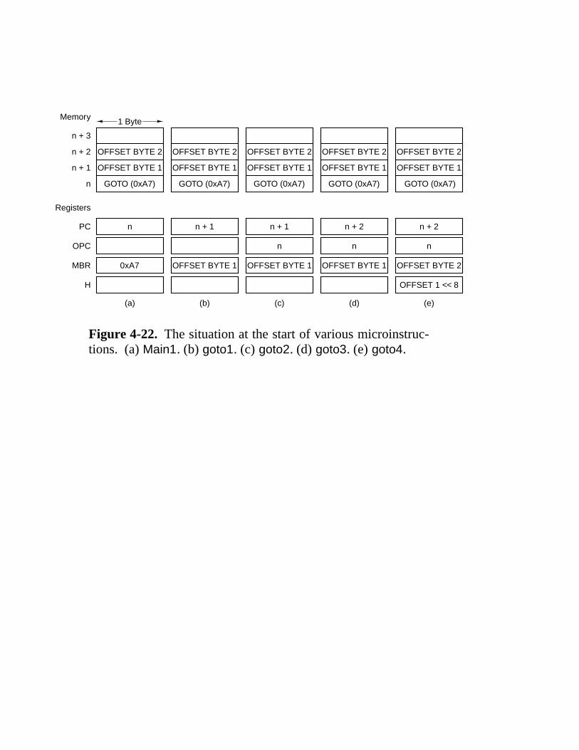
Memory 1 Byte
n + 3
n + 2
n + 1
n
OFFSET BYTE 2
OFFSET BYTE 1
GOTO (0xA7)
OFFSET BYTE 2
OFFSET BYTE 1
GOTO (0xA7)
OFFSET BYTE 2
OFFSET BYTE 1
GOTO (0xA7)
OFFSET BYTE 2
OFFSET BYTE 1
GOTO (0xA7)
OFFSET BYTE 2
OFFSET BYTE 1
GOTO (0xA7)
Registers
PC
OPC
MBR
H
n
n n n
n + 1 n + 1 n + 2 n + 2
OFFSET BYTE 1 OFFSET BYTE 2OFFSET BYTE 1 OFFSET BYTE 10xA7
OFFSET 1 << 8
(a) (b) (c) (d) (e)
Figure 4-22. The situation at the start of various microinstruc-tions. (a) Main1. (b) goto1. (c) goto2. (d) goto3. (e) goto4.

22222222222222222222222222222222222222222222222222222222222222222222222222222222Label Operations Comments22222222222222222222222222222222222222222222222222222222222222222222222222222222pop1 MAR = SP = SP − 1; rd Read in next-to-top word on stackpop2 Wait for new TOS to be read from memorypop3 TOS = MDR; goto Main1 Copy new word to TOSMain1 PC = PC + 1; fetch; goto (MBR) MBR holds opcode; get next byte; dispatch222222222222222222222222222222222222222222222222222222222222222222222222222222221111111
1111111
Figure 4-23. New microprogram sequence for executing POP.

222222222222222222222222222222222222222222222222222222222222222222222222222222Label Operations Comments222222222222222222222222222222222222222222222222222222222222222222222222222222pop1 MAR = SP = SP − 1; rd Read in next-to-top word on stackMain1.pop PC = PC + 1; fetch MBR holds opcode; fetch next bytepop3 TOS = MDR; goto (MBR) Copy new word to TOS; dispatch on opcode222222222222222222222222222222222222222222222222222222222222222222222222222222111111
111111
Figure 4-24. Enhanced microprogram sequence for executingPOP.
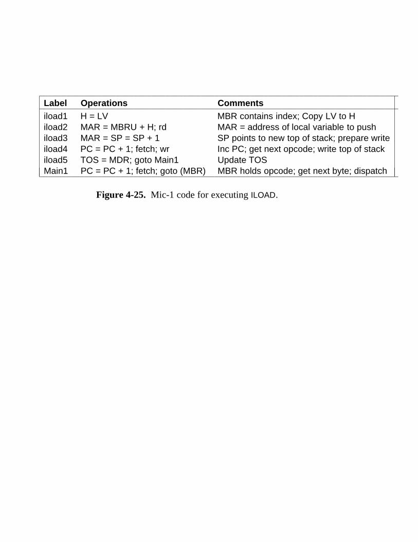
22222222222222222222222222222222222222222222222222222222222222222222222222222222Label Operations Comments22222222222222222222222222222222222222222222222222222222222222222222222222222222iload1 H = LV MBR contains index; Copy LV to Hiload2 MAR = MBRU + H; rd MAR = address of local variable to pushiload3 MAR = SP = SP + 1 SP points to new top of stack; prepare writeiload4 PC = PC + 1; fetch; wr Inc PC; get next opcode; write top of stackiload5 TOS = MDR; goto Main1 Update TOSMain1 PC = PC + 1; fetch; goto (MBR) MBR holds opcode; get next byte; dispatch222222222222222222222222222222222222222222222222222222222222222222222222222222221111111111
1111111111
Figure 4-25. Mic-1 code for executing ILOAD.

22222222222222222222222222222222222222222222222222222222222222222222222222222222Label Operations Comments22222222222222222222222222222222222222222222222222222222222222222222222222222222iload1 MAR = MBRU + LV; rd MAR = address of local variable to pushiload2 MAR = SP = SP + 1 SP points to new top of stack; prepare writeiload3 PC = PC + 1; fetch; wr Inc PC; get next opcode; write top of stackiload4 TOS = MDR Update TOSiload5 PC = PC + 1; fetch; goto (MBR) MBR already holds opcode; fetch index byte2222222222222222222222222222222222222222222222222222222222222222222222222222222211111111
11111111
Figure 4-26. Three-bus code for executing ILOAD.

MBR2
Shift registerFrom memory
MBR1
+1
Write PC
2 low-order bitsB busC bus
IMAR
PC
+1, 2
Figure 4-27. A fetch unit for the Mic-1.
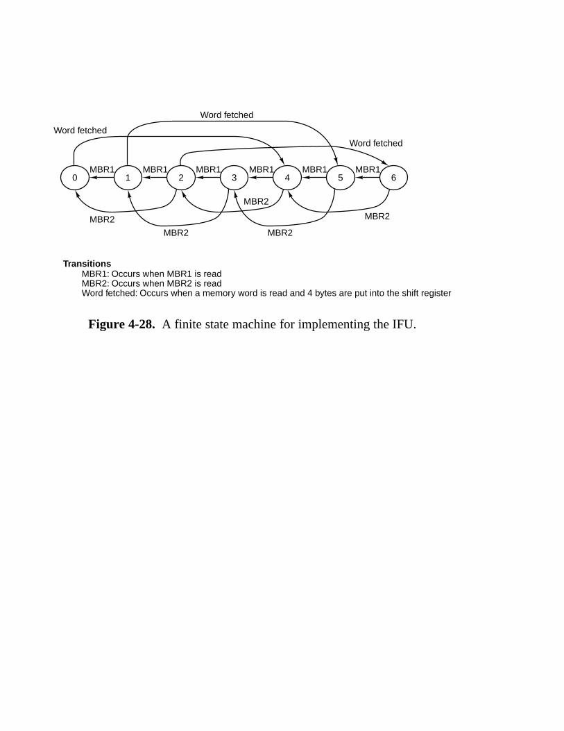
Word fetched
Word fetched
Word fetched
0MBR1
MBR2
MBR2
MBR2 MBR2
MBR2
TransitionsMBR1: Occurs when MBR1 is readMBR2: Occurs when MBR2 is readWord fetched: Occurs when a memory word is read and 4 bytes are put into the shift register
1MBR1
2MBR1
3MBR1
4MBR1
5MBR1
6
Figure 4-28. A finite state machine for implementing the IFU.

H
Shifter
ALUN
B bus
C bus
6ALUcontrol
Control signals
Memorycontrolregisters
Enable onto B bus
Write C bus to register
Toandfrommainmemory
Z
MBR2
SP
LV
CPP
TOS
PC
MDR
MAR
MBR
OPC
Instructionfetch unit(IFU)
A bus
Figure 4-29. The datapath for Mic-2.

Label Operations Comments22222222222222222222222222222222222222222222222222222222222222222222222222222222222222222222nop1 goto (MBR) Branch to next instruction22222222222222222222222222222222222222222222222222222222222222222222222222222222222222222222iadd1 MAR = SP = SP − 1; rd Read in next-to-top word on stackiadd2 H = TOS H = top of stackiadd3 MDR = TOS = MDR+H; wr; goto (MBR1) Add top two words; write to new top of stack22222222222222222222222222222222222222222222222222222222222222222222222222222222222222222222isub1 MAR = SP = SP − 1; rd Read in next-to-top word on stackisub2 H = TOS H = top of stackisub3 MDR = TOS = MDR−H; wr; goto (MBR1) Subtract TOS from Fetched TOS-122222222222222222222222222222222222222222222222222222222222222222222222222222222222222222222iand1 MAR = SP = SP − 1; rd Read in next-to-top word on stackiand2 H = TOS H = top of stackiand3 MDR = TOS = MDR AND H; wr; goto (MBR1) AND Fetched TOS-1 with TOS22222222222222222222222222222222222222222222222222222222222222222222222222222222222222222222ior1 MAR = SP = SP − 1; rd Read in next-to-top word on stackior2 H = TOS H = top of stackior3 MDR = TOS = MDR OR H; wr; goto (MBR1) OR Fetched TOS-1 with TOS22222222222222222222222222222222222222222222222222222222222222222222222222222222222222222222dup1 MAR = SP = SP + 1 Increment SP; copy to MARdup2 MDR = TOS; wr; goto (MBR1) Write new stack word22222222222222222222222222222222222222222222222222222222222222222222222222222222222222222222pop1 MAR = SP = SP − 1; rd Read in next-to-top word on stackpop2 Wait for readpop3 TOS = MDR; goto (MBR1) Copy new word to TOS22222222222222222222222222222222222222222222222222222222222222222222222222222222222222222222swap1 MAR = SP − 1; rd Read 2nd word from stack; set MAR to SPswap2 MAR = SP Prepare to write new 2nd wordswap3 H = MDR; wr Save new TOS; write 2nd word to stackswap4 MDR = TOS Copy old TOS to MDRswap5 MAR = SP − 1; wr Write old TOS to 2nd place on stackswap6 TOS = H; goto (MBR1) Update TOS22222222222222222222222222222222222222222222222222222222222222222222222222222222222222222222bipush1 SP = MAR = SP + 1 Set up MAR for writing to new top of stackbipush2 MDR = TOS = MBR1; wr; goto (MBR1) Update stack in TOS and memory22222222222222222222222222222222222222222222222222222222222222222222222222222222222222222222iload1 MAR = LV + MBR1U; rd Move LV + index to MAR; read operandiload2 MAR = SP = SP + 1 Increment SP; Move new SP to MARiload3 TOS = MDR; wr; goto (MBR1) Update stack in TOS and memory22222222222222222222222222222222222222222222222222222222222222222222222222222222222222222222istore1 MAR = LV + MBR1U Set MAR to LV + indexistore2 MDR = TOS; wr Copy TOS for storingistore3 MAR = SP = SP − 1; rd Decrement SP; read new TOSistore4 Wait for readistore5 TOS = MDR; goto (MBR1) Update TOS22222222222222222222222222222222222222222222222222222222222222222222222222222222222222222222wide1 goto (MBR1 OR 0x100) Next address is 0x100 Ored with opcode22222222222222222222222222222222222222222222222222222222222222222222222222222222222222222222wide3iload1 MAR = LV + MBR2U; rd; goto iload2 Identical to iload1 but using 2-byte index22222222222222222222222222222222222222222222222222222222222222222222222222222222222222222222wide3istore1 MAR = LV + MBR2U; goto istore2 Identical to istore1 but using 2-byte index22222222222222222222222222222222222222222222222222222222222222222222222222222222222222222222ldc3w1 MAR = CPP + MBR2U; rd; goto iload2 Same as wide3iload1 but indexing off CPP22222222222222222222222222222222222222222222222222222222222222222222222222222222222222222222

iinc1 MAR = LV + MBR1U; rd Set MAR to LV + index for readiinc2 H = MBR1 Set H to constantiinc3 MDR = MDR + H; wr; goto (MBR1) Increment by constant and update22222222222222222222222222222222222222222222222222222222222222222222222222222222222222222222goto1 H = PC − 1 Copy PC to Hgoto2 PC = H + MBR2 Add offset and update PCgoto3 Have to wait for IFU to fetch new opcodegoto4 goto (MBR1) Dispatch to next instruction22222222222222222222222222222222222222222222222222222222222222222222222222222222222222222222iflt1 MAR = SP = SP − 1; rd Read in next-to-top word on stackiflt2 OPC = TOS Save TOS in OPC temporarilyiflt3 TOS = MDR Put new top of stack in TOSiflt4 N = OPC; if (N) goto T; else goto F Branch on N bit
Figure 4-30. The microprogram for the Mic-2 (part 1 of 2).
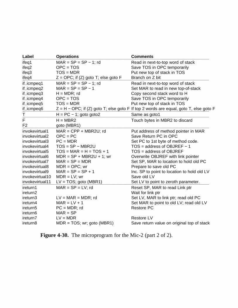
Label Operations Comments222222222222222222222222222222222222222222222222222222222222222222222222222222222222222ifeq1 MAR = SP = SP − 1; rd Read in next-to-top word of stackifeq2 OPC = TOS Save TOS in OPC temporarilyifeq3 TOS = MDR Put new top of stack in TOSifeq4 Z = OPC; if (Z) goto T; else goto F Branch on Z bit222222222222222222222222222222222222222222222222222222222222222222222222222222222222222if3icmpeq1 MAR = SP = SP − 1; rd Read in next-to-top word of stackif3icmpeq2 MAR = SP = SP − 1 Set MAR to read in new top-of-stackif3icmpeq3 H = MDR; rd Copy second stack word to Hif3icmpeq4 OPC = TOS Save TOS in OPC temporarilyif3icmpeq5 TOS = MDR Put new top of stack in TOSif3icmpeq6 Z = H − OPC; if (Z) goto T; else goto F If top 2 words are equal, goto T, else goto F222222222222222222222222222222222222222222222222222222222222222222222222222222222222222T H = PC − 1; goto goto2 Same as goto1222222222222222222222222222222222222222222222222222222222222222222222222222222222222222F H = MBR2 Touch bytes in MBR2 to discardF2 goto (MBR1)222222222222222222222222222222222222222222222222222222222222222222222222222222222222222invokevirtual1 MAR = CPP + MBR2U; rd Put address of method pointer in MARinvokevirtual2 OPC = PC Save Return PC in OPCinvokevirtual3 PC = MDR Set PC to 1st byte of method code.invokevirtual4 TOS = SP − MBR2U TOS = address of OBJREF − 1invokevirtual5 TOS = MAR = H = TOS + 1 TOS = address of OBJREFinvokevirtual6 MDR = SP + MBR2U + 1; wr Overwrite OBJREF with link pointerinvokevirtual7 MAR = SP = MDR Set SP, MAR to location to hold old PCinvokevirtual8 MDR = OPC; wr Prepare to save old PCinvokevirtual9 MAR = SP = SP + 1 Inc. SP to point to location to hold old LVinvokevirtual10 MDR = LV; wr Save old LVinvokevirtual11 LV = TOS; goto (MBR1) Set LV to point to zeroth parameter.222222222222222222222222222222222222222222222222222222222222222222222222222222222222222ireturn1 MAR = SP = LV; rd Reset SP, MAR to read Link ptrireturn2 Wait for link ptrireturn3 LV = MAR = MDR; rd Set LV, MAR to link ptr; read old PCireturn4 MAR = LV + 1 Set MAR to point to old LV; read old LVireturn5 PC = MDR; rd Restore PCireturn6 MAR = SPireturn7 LV = MDR Restore LVireturn8 MDR = TOS; wr; goto (MBR1) Save return value on original top of stack
Figure 4-30. The microprogram for the Mic-2 (part 2 of 2).
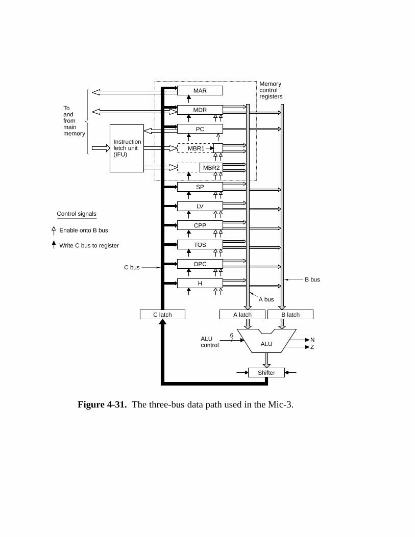
H
A latchC latch B latch
Shifter
ALUN
B bus
C bus
6ALUcontrol
Control signals
Memorycontrolregisters
Enable onto B bus
Write C bus to register
Toandfrommainmemory
Z
MBR2
SP
LV
CPP
TOS
PC
MDR
MAR
MBR1
OPC
Instructionfetch unit(IFU)
A bus
Figure 4-31. The three-bus data path used in the Mic-3.

22222222222222222222222222222222222222222222222222222222222222222222222222222222Label Operations Comments22222222222222222222222222222222222222222222222222222222222222222222222222222222swap1 MAR = SP − 1; rd Read 2nd word from stack; set MAR to SPswap2 MAR = SP Prepare to write new 2nd wordswap3 H = MDR; wr Save new TOS; write 2nd word to stackswap4 MDR = TOS Copy old TOS to MDRswap5 MAR = SP − 1; wr Write old TOS to 2nd place on stackswap6 TOS = H; goto (MBR1) Update TOS22222222222222222222222222222222222222222222222222222222222222222222222222222222111111111
111111111
Figure 4-32. The Mic-2 code for SWAP.

222222222222222222222222222222222222222222222222222222222222222222222222222222222Swap1 Swap2 Swap3 Swap4 Swap5 Swap6222222222222222222222222222222222222222222222222222222222222222222222222222222222
Cy MAR=SP−1;rd MAR=SP H=MDR;wr MDR=TOS MAR=SP−1;wr TOS=H;goto (MBR1)2222222222222222222222222222222222222222222222222222222222222222222222222222222221 B=SP2222222222222222222222222222222222222222222222222222222222222222222222222222222222 C=B−1 B=SP2222222222222222222222222222222222222222222222222222222222222222222222222222222223 MAR=C; rd C=B2222222222222222222222222222222222222222222222222222222222222222222222222222222224 MDR=mem MAR=C2222222222222222222222222222222222222222222222222222222222222222222222222222222225 B=MDR2222222222222222222222222222222222222222222222222222222222222222222222222222222226 C=B B=TOS2222222222222222222222222222222222222222222222222222222222222222222222222222222227 H=C; wr C=B B=SP2222222222222222222222222222222222222222222222222222222222222222222222222222222228 Mem=MDR MDR=C C=B−1 B=H2222222222222222222222222222222222222222222222222222222222222222222222222222222229 MAR=C; wr C=B222222222222222222222222222222222222222222222222222222222222222222222222222222222
10 Mem=MDR TOS=C22222222222222222222222222222222222222222222222222222222222222222222222222222222211 goto (MBR1)22222222222222222222222222222222222222222222222222222222222222222222222222222222211
111111111111111111
11111111111111111111
11111111111111111111
11111111111111111111
11111111111111111111
11111111111111111111
11111111111111111111
11111111111111111111
Figure 4-33. The implementation of SWAP on the Mic-3.

1
Inst
ruct
ion
Cycle 1 Cycle 2
Ti me
Cycle 3 Cycle 4
IFU
ALU
Reg
Shifter
AC B
IFU
ALU
Reg
Shifter
AC B
IFU
ALU
Reg
Shifter
AC B
IFU
ALU
Reg
Shifter
AC B
IFU
ALU
Reg
Shifter
AC B
IFU
ALU
Reg
Shifter
AC B
IFU
ALU
Reg
Shifter
AC B
IFU
ALU
Reg
Shifter
AC B
IFU
ALU
Reg
Shifter
AC B
IFU
ALU
Reg
Shifter
AC B
2
IFU
ALU
Reg
Shifter
AC B
IFU
ALU
Reg
Shifter
AC B
IFU
ALU
Reg
Shifter
AC B
3
IFU
ALU
Reg
Shifter
AC B
IFU
ALU
Reg
Shifter
AC B4
IFU
ALU
Reg
Shifter
AC B
Figure 4-34. Graphical illustration of how a pipeline works.
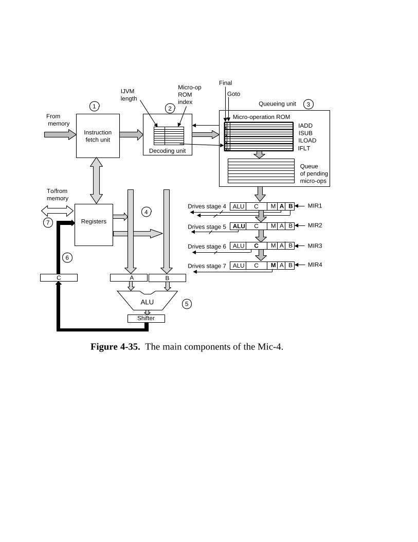
ALU
BC
Shifter
A
Registers
Queueing unit
IADDISUBILOADIFLT
Micro-operation ROM
Instructionfetch unit
From memory
IJVMlength
Micro-opROMindex
Decoding unit
Queueof pendingmicro-ops
Final
Goto
1 23
4
5
6
7
To/frommemory
ALU C M A B
ALU C M A B
ALU C M A B
ALU C M A B
Drives stage 4
Drives stage 5
Drives stage 6
Drives stage 7
MIR1
MIR2
MIR4
MIR3
Figure 4-35. The main components of the Mic-4.
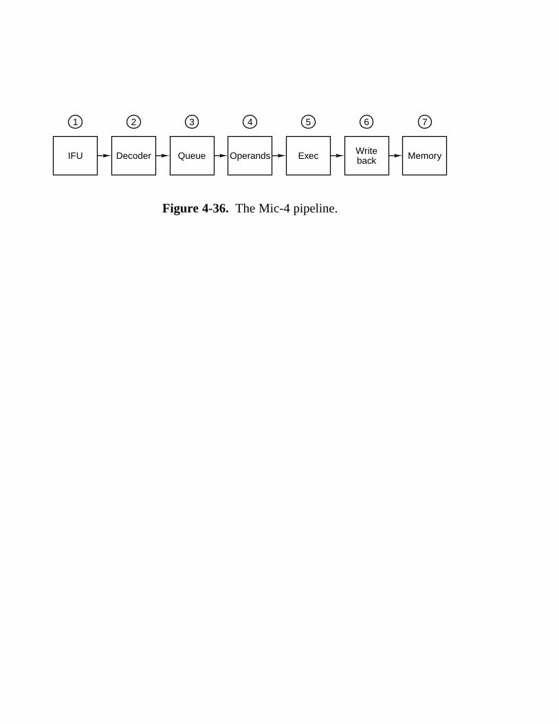
1
IFU
2
Decoder
3
Queue
4
Operands
5
Exec
6
Writeback
7
Memory
Figure 4-36. The Mic-4 pipeline.

Processorboard
CPUpackage CPU chip
Keyboardcontroller
Graphicscontroller
Diskcontroller
Mainmemory(DRAM)
L1-I L1-D
UnifiedL2cache
UnifiedL3 cache
Split L1 instruction and data caches Board-level cache (SRAM)
Figure 4-37. A system with three levels of cache.

Valid
Entry
2047
Tag DataAddresses that use this entry
(a)
(b)
Bits 16 11 3 2
TAG LINE WORD BYTE
65504-65535, 131040-131072, …
96-127, 65632-65663, 131068-13109964-95, 65600-65631, 131036-131067, …32-63, 65568-65599, 131004-131035, … 0-31, 65536-65567, 131072-131003, …
76543210
Figure 4-38. (a) A direct-mapped cache. (b) A 32-bit virtual address.

Valid
Tag Data2047
76543210
Entry A
Valid
Tag Data
Entry B
Valid
Tag Data
Entry C
Valid
Tag Data
Entry D
Figure 4-39. A four-way associative cache.
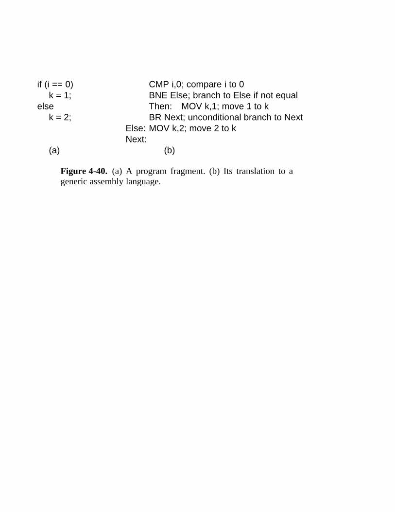
if (i == 0) CMP i,0; compare i to 0k = 1; BNE Else; branch to Else if not equal
else Then: MOV k,1; move 1 to kk = 2; BR Next; unconditional branch to Next
Else: MOV k,2; move 2 to kNext:
(a) (b)
Figure 4-40. (a) A program fragment. (b) Its translation to ageneric assembly language.

Valid
6543210
Branch/no branch
SlotBranchaddress/tag
Targetaddress
(a)
Valid
6543210
Predictionbits
SlotBranchaddress/tag
(c)
Valid
6543210
PredictionbitsSlot
Branchaddress/tag
(b)
Figure 4-41. (a) A 1-bit branch history. (b) A 2-bit branch his-tory. (c) A mapping between branch instruction address andtarget address.

No branch
Branch
Branch
00
Nobranch
Predictno branch
01
Predictno branchone more
time
10
Predictbranch
one moretime
Branch
Nobranch
Branch
No branch
11
Predictbranch
Figure 4-42. A 2-bit finite-state machine for branch prediction.
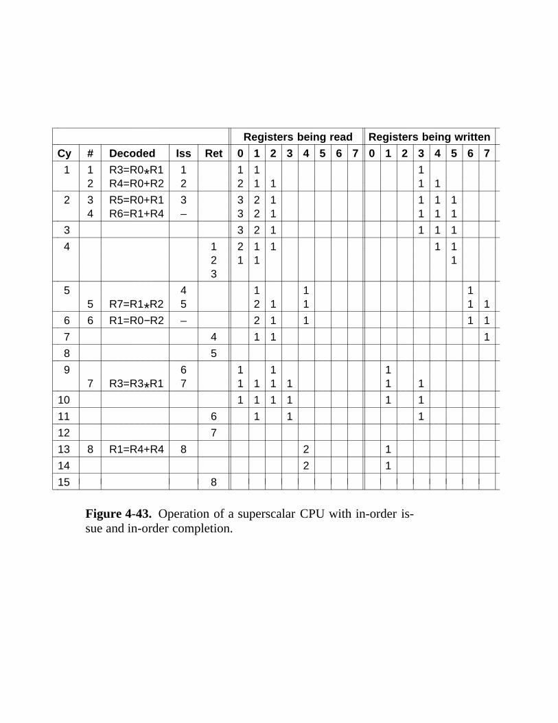
222222222222222222222222222222222222222222222222222222222222222222222222222222222Registers being read Registers being written222222222222222222222222222222222222222222222222222222222222222222222222222222222
Cy # Decoded Iss Ret 0 1 2 3 4 5 6 7 0 1 2 3 4 5 6 72222222222222222222222222222222222222222222222222222222222222222222222222222222221 1 R3=R0*R1 1 1 1 1
2 R4=R0+R2 2 2 1 1 1 12222222222222222222222222222222222222222222222222222222222222222222222222222222222 3 R5=R0+R1 3 3 2 1 1 1 1
4 R6=R1+R4 – 3 2 1 1 1 12222222222222222222222222222222222222222222222222222222222222222222222222222222223 3 2 1 1 1 12222222222222222222222222222222222222222222222222222222222222222222222222222222224 1 2 1 1 1 1
2 1 1 13222222222222222222222222222222222222222222222222222222222222222222222222222222222
5 4 1 1 15 R7=R1*R2 5 2 1 1 1 1222222222222222222222222222222222222222222222222222222222222222222222222222222222
6 6 R1=R0−R2 – 2 1 1 1 12222222222222222222222222222222222222222222222222222222222222222222222222222222227 4 1 1 12222222222222222222222222222222222222222222222222222222222222222222222222222222228 52222222222222222222222222222222222222222222222222222222222222222222222222222222229 6 1 1 1
7 R3=R3*R1 7 1 1 1 1 1 122222222222222222222222222222222222222222222222222222222222222222222222222222222210 1 1 1 1 1 122222222222222222222222222222222222222222222222222222222222222222222222222222222211 6 1 1 122222222222222222222222222222222222222222222222222222222222222222222222222222222212 722222222222222222222222222222222222222222222222222222222222222222222222222222222213 8 R1=R4+R4 8 2 122222222222222222222222222222222222222222222222222222222222222222222222222222222214 2 122222222222222222222222222222222222222222222222222222222222222222222222222222222215 8222222222222222222222222222222222222222222222222222222222222222222222222222222222111111111111111111111111111111111
11111111111111111111111111111111
11111111111111111111111111111111
11111111111111111111111111111111
11111111111111111111111111111111
111111111111111111111111111111111
111111111111111111111111111111111
11111111111111111111111111111111
11111111111111111111111111111111
11111111111111111111111111111111
11111111111111111111111111111111
11111111111111111111111111111111
11111111111111111111111111111111
11111111111111111111111111111111
111111111111111111111111111111111
111111111111111111111111111111111
11111111111111111111111111111111
11111111111111111111111111111111
11111111111111111111111111111111
11111111111111111111111111111111
11111111111111111111111111111111
11111111111111111111111111111111
11111111111111111111111111111111
111111111111111111111111111111111
Figure 4-43. Operation of a superscalar CPU with in-order is-sue and in-order completion.

222222222222222222222222222222222222222222222222222222222222222222222222222222222Registers being read Registers being written222222222222222222222222222222222222222222222222222222222222222222222222222222222
Cy # Decoded Iss Ret 0 1 2 3 4 5 6 7 0 1 2 3 4 5 6 72222222222222222222222222222222222222222222222222222222222222222222222222222222221 1 R3=R0*R1 1 1 1 1
2 R4=R0+R2 2 2 1 1 1 12222222222222222222222222222222222222222222222222222222222222222222222222222222222 3 R5=R0+R1 3 3 2 1 1 1 1
4 R6=R1+R4 – 3 2 1 1 1 12222222222222222222222222222222222222222222222222222222222222222222222222222222223 5 R7=R1*R2 5 3 3 2 1 1 1 1
6 S1=R0−R2 6 4 3 3 1 1 1 12 3 3 2 1 1 1222222222222222222222222222222222222222222222222222222222222222222222222222222222
4 4 3 4 2 1 1 1 1 17 R3=R3*S1 – 3 4 2 1 1 1 1 18 S2=R4+R4 8 3 4 2 3 1 1 1 1
1 2 3 2 3 1 1 13 1 2 2 3 1 1222222222222222222222222222222222222222222222222222222222222222222222222222222222
5 6 2 1 3 1 1 12222222222222222222222222222222222222222222222222222222222222222222222222222222226 7 2 1 1 3 1 1 1 1
4 1 1 1 2 1 1 15 1 2 1 18 1 1222222222222222222222222222222222222222222222222222222222222222222222222222222222
7 1 12222222222222222222222222222222222222222222222222222222222222222222222222222222228 1 12222222222222222222222222222222222222222222222222222222222222222222222222222222229 722222222222222222222222222222222222222222222222222222222222222222222222222222222211
11111111111111111111111111111
11111111111111111111111111111
11111111111111111111111111111
11111111111111111111111111111
11111111111111111111111111111
1111111111111111111111111111111
1111111111111111111111111111111
11111111111111111111111111111
11111111111111111111111111111
11111111111111111111111111111
11111111111111111111111111111
11111111111111111111111111111
11111111111111111111111111111
11111111111111111111111111111
1111111111111111111111111111111
1111111111111111111111111111111
11111111111111111111111111111
11111111111111111111111111111
11111111111111111111111111111
11111111111111111111111111111
11111111111111111111111111111
11111111111111111111111111111
11111111111111111111111111111
1111111111111111111111111111111
Figure 4-44. Operation of a superscalar CPU with out-of-order issue and out-of-order completion.

evensum = 0;
oddsum = 0;
i = 0;
while (i < limit) {
k = i * i * i;k = i * i * i;
if ((i/2) * 2) == 0)
evensum = evensum + k;
else
oddsum = oddsum + k;
}(a) (b)
evensum = 0;
oddsum = 0;
i = 0;
while (i < limit)
if ((i/2) * 2) = = 0)
T F
evensum = evensum + k; oddsum = oddsum + k;
i = i + 1;i = i + 1;
i >= limit
Figure 4-45. (a) A program fragment. (b) The correspondingbasic block graph.
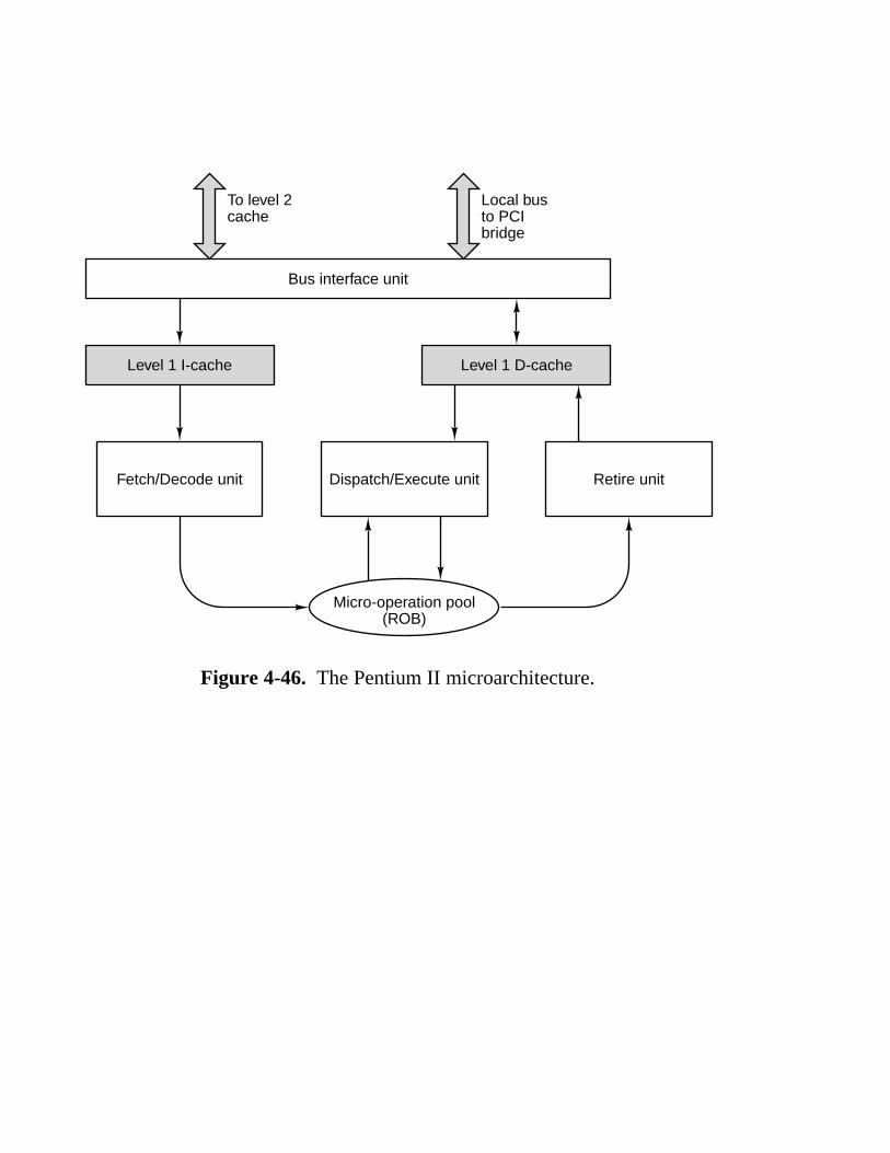
Local busto PCIbridge
To level 2cache
Bus interface unit
Level 1 I-cache Level 1 D-cache
Fetch/Decode unit Dispatch/Execute unit Retire unit
Micro-operation pool(ROB)
Figure 4-46. The Pentium II microarchitecture.

RAT
Level 1 I-cache
Pipeline stage
IFU0
IFU1
IFU2
ID0
ID1
ROB
Cache line fetcher
Instruction length decoder
Instruction aligner
0 1 2
Micro-operation queuer
Register allocator
Micro-operations go in the ROB
Staticbranch predictor
Micro-operationsequencer
Dynamicbranch predictor
Next IP
Figure 4-47. Internal structure of the Fetch/Decode unit (simplified).

MMXExecutionunit
Floating-Pointexecution unit
From/toROB
Reservationstation
Port 0
Port 1
Port 2
Port 3
Port 4
MMXExecutionunit
Floating-Pointexecution unit
Integerexecution unit
Integerexecution unit
LoadUnit
StoreUnit
StoreUnit
Loads
Stores
Stores
Figure 4-48. The Dispatch/Execute unit.

To mainmemory
Memory interface unit
External cache unitLevel 2 cache
Level 1 cache
Prefetch/Dispatch unit
Grouping logic
Integer execution unit
Integer registers
ALU ALU FP ALU FP ALU
Floating-point unit
FP registers
Graphics unit
Load/store unit
Loadstore
Storequeue
Level 1 D-cache
Figure 4-49. The UltraSPARC II microarchitecture.

Integer pipeline
Fetch Decode Group
Execute Cache
Register
Write
Floating-point/graphics pipeline
N1 N2
N3
X1 X2 X3
Figure 4-50. The UltraSPARC II’s pipeline.

Execution control
unit
Integer andfloating-point
unit
64 32-Bit registers for holdingthe top 64 words of the stack
3 x 32
Prefetch,decode, and folding unit
0-16 KBData
cache
0-16 KBInstruction
cache
32 32
Memory and I/O bus interface unit
32 32
2 x 32
Figure 4-51. The block diagram of the picoJava II with bothlevel 1 caches and the floating-point unit. This is configurationof the microJava 701.
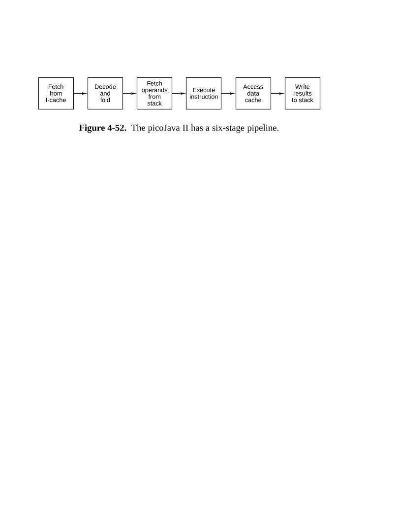
Fetchfrom
I-cache
Decodeandfold
Fetchoperands
fromstack
Executeinstruction
Accessdata
cache
Writeresultsto stack
Figure 4-52. The picoJava II has a six-stage pipeline.
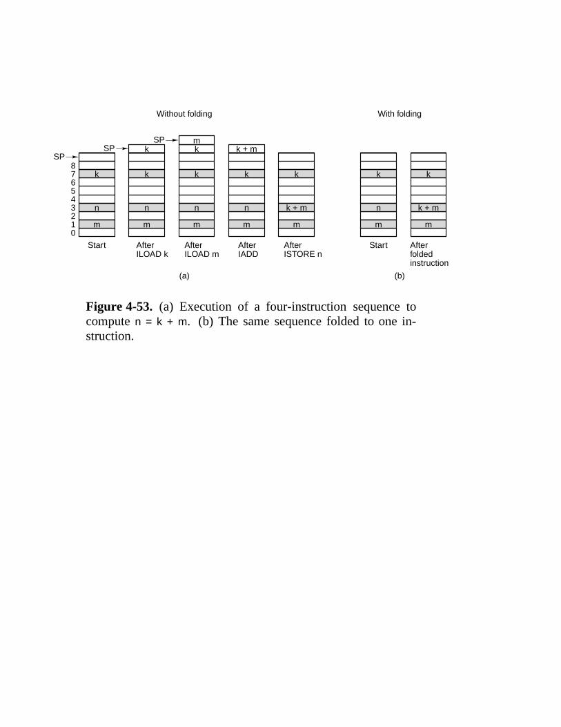
Without folding With folding
SP
876543210
Start AfterILOAD k
AfterILOAD m
AfterIADD
AfterISTORE n
Start Afterfoldedinstruction
(a) (b)
SP
SP
m m m m m m m
n n n n k + m n k + m
k k
k km
k + m
k k k k k
Figure 4-53. (a) Execution of a four-instruction sequence tocompute n = k + m. (b) The same sequence folded to one in-struction.

22222222222222222222222222222222222222222222222222222222222222222222222222222222Group Description Example22222222222222222222222222222222222222222222222222222222222222222222222222222222NF Nonfoldable instructions GOTO22222222222222222222222222222222222222222222222222222222222222222222222222222222LV Pushing a word onto the stack ILOAD22222222222222222222222222222222222222222222222222222222222222222222222222222222MEM Popping a word and storing it in memory ISTORE22222222222222222222222222222222222222222222222222222222222222222222222222222222BG1 Operations using one stack operand IFEQ22222222222222222222222222222222222222222222222222222222222222222222222222222222BG2 Operations using two stack operands IF3CMPEQ22222222222222222222222222222222222222222222222222222222222222222222222222222222OP Computations on two operands with one result IADD222222222222222222222222222222222222222222222222222222222222222222222222222222221111111111
1111111111
1111111111
1111111111
Figure 4-54. JVM instruction groups for folding purposes.

222222222222222222222222222222222222222222222222222222222222222222222222222Instruction sequence Example222222222222222222222222222222222222222222222222222222222222222222222222222
LV LV OP MEM ILOAD, ILOAD, IADD, ISTORE222222222222222222222222222222222222222222222222222222222222222222222222222LV LV OP ILOAD, ILOAD, IADD222222222222222222222222222222222222222222222222222222222222222222222222222LV LV BG2 ILOAD, ILOAD, IF3CMPEQ222222222222222222222222222222222222222222222222222222222222222222222222222LV BG1 ILOAD, IFEQ222222222222222222222222222222222222222222222222222222222222222222222222222LV BG2 ILOAD, IF3CMPEQ222222222222222222222222222222222222222222222222222222222222222222222222222LV MEM ILOAD, ISTORE222222222222222222222222222222222222222222222222222222222222222222222222222OP MEM IADD, ISTORE222222222222222222222222222222222222222222222222222222222222222222222222222111111111111
1111111111
1111111111
1111111111
111111111111
111111111111
Figure 4-55. Some of the JVM instruction sequences that can be folded.

264 THE MICROARCHITECTURE LEVEL CHAP. 4
4.5 IMPROVING PERFORMANCE
All computer manufacturers want their systems to run as fast as possible. Inthis section, we will look at a number of advanced techniques currently beinginvestigated to improve system (primarily CPU and memory) performance. Dueto the highly competitive nature of the computer industry, the lag between newresearch ideas that can make a computer faster and their incorporation into pro-ducts is surprisingly short. Consequently, most of the ideas we will discuss arealready in use in a wide variety of existing products.
The ideas to be discussed fall into two rough categories: implementationimprovements and architectural improvements. Implementation improvementsare ways of building a new CPU or memory to make the system run faster withoutchanging the architecture. Modifying the implementation without changing thearchitecture means that old programs will run on the new machine, a major sellingpoint. One way to improve the implementation is to use a faster clock, but this isnot the only way. The performance gains from the 80386 through the 80486, Pen-tium, and Pentium Pro, to the Pentium II are due to better implementations, as thearchitecture has remained essentially the same through all of them.
Some kinds of improvements can be made only by changing the architecture.Sometimes these changes are incremental, such as adding new instructions orregisters, so that old programs will continue to run on the new models. In thiscase, to get the full performance, the software must be changed, or at least recom-piled with a new compiler that takes advantage of the new features.
However, once in a few decades, designers realize that the old architecturehas outlived its usefulness and that the only way to make progress is start all overagain. The RISC revolution in the 1980s was one such breakthrough; another oneis in the air now. We will look at one example (the Intel IA-64) in Chap. 5.
In the rest of this section we will look at four different techniques for improv-ing CPU performance. We will start with three well-established implementationimprovements and then move on to one that needs a little architectural support towork best. These techniques are cache memory, branch prediction, out-of-orderexecution with register renaming, and speculative execution.
4.5.1 Cache Memory
One of the most challenging aspects of computer design throughout historyhas been to provide a memory system able to provide operands to the processor atthe speed it can process them. The recent high rate of growth in processor speedhas not been accompanied by a corresponding speedup in memories. Relative toCPUs, memories have been getting slower for decades. Given the enormousimportance of primary memory, this situation has greatly limited the developmentof high-performance systems, and has stimulated research on ways to get aroundthe problem of memory speeds that are much slower than CPU speeds, an

SEC. 4.5 IMPROVING PERFORMANCE 265
relatively speaking, getting worse every year.Modern processors place overwhelming demands on a memory system, both
in terms of latency (the delay in supplying an operand) and bandwidth (theamount of data supplied per unit of time). Unfortunately, these two aspects of amemory system are largely at odds. Many techniques for increasing bandwidth doso only by increasing latency. For example, the pipelining techniques used in theMic-3 can be applied to a memory system, with multiple, overlapping memoryrequests handled efficiently. Unfortunately, as with the Mic-3, this results ingreater latency for individual memory operations. As processor clock speeds getfaster, it becomes more and more difficult to provide a memory system capable ofsupplying operands in one or two clock cycles.
One way to attack this problem is by providing caches. As we saw in Sec.2.2.5, a cache holds the most recently used memory words in a small, fastmemory, speeding up access to them. If a large enough percentage of the memorywords needed are in the cache, the effective memory latency can be reduced enor-mously.
One of the most effective techniques for improving both bandwidth andlatency comes from the use of multiple caches. A basic technique that works veryeffectively is to introduce a separate cache for instructions and data. There areseveral benefits from having separate caches for instructions and data, often calleda split cache. First, memory operations can be initiated independently in eachcache, effectively doubling the bandwidth of the memory system. This is the rea-son that it makes sense to provide two separate memory ports, as we did in theMic-1: each port has its own cache. Note that each cache has independent accessto the main memory.
Today, many memory systems are more complicated than this, and an addi-tional cache, called a level 2 cache, may reside between the instruction and datacaches and main memory. In fact, there may be three or more levels of cache asmore sophisticated memory systems are required. In Fig. 4-1 we see a systemwith three levels of cache. The CPU chip itself contains a small instruction cacheand a small data cache, typically 16 KB to 64 KB. Then there is the level 2 cache,which is not on the CPU chip, but may be included in the CPU package, next tothe CPU chip and connected to it by a high-speed path. This cache is generallyunified, containing a mixture of data and instructions. A typical size for the L2cache is 512 KB to 1 MB. The third-level cache is on the processor board andconsists of a few megabytes of SRAM, which is much faster than the mainDRAM memory. Caches are generally inclusive, with the full contents of thelevel 1 cache being in the level 2 cache and the full contents of the level 2 cachebeing in the level 3 cache.
Caches depend on two kinds of address locality to achieve their goal. Spatiallocality is the observation that memory locations with addresses numerically simi-lar to a recently accessed memory location are likely to be accessed in the nearfuture. Caches exploit this property by bringing in more data than have been

266 THE MICROARCHITECTURE LEVEL CHAP. 4
Processorboard
CPUpackage CPU chip
Keyboardcontroller
Graphicscontroller
Diskcontroller
Mainmemory(DRAM)
L1-I L1-D
UnifiedL2cache
UnifiedL3 cache
Split L1 instruction and data caches Board-level cache (SRAM)
Figure 4-1. A system with three levels of cache.
requested, with the expectation that future requests can be anticipated. Temporallocality occurs when recently accessed memory locations are accessed again.This may occur, for example, to memory locations near the top of the stack, orinstructions inside a loop. Temporal locality is exploited in cache designs pri-marily by the choice of what to discard on a cache miss. Many cache replacementalgorithms exploit temporal locality by discarding those entries that have not beenrecently accessed.
All caches use the following model. Main memory is divided up into fixed-size blocks called cache lines. A cache line typically consists of 4 to 64 consecu-tive bytes. Lines are numbered consecutively starting at 0, so with a 32-byte linesize, line 0 is bytes 0 to 31, line 1 is bytes 32 to 63, and so on. At any instant,some lines are in the cache. When memory is referenced, the cache controller cir-cuit checks to see if the word referenced is currently in the cache. If so, the valuethere can be used, saving a trip to main memory. If the word is not there, someline entry is removed from the cache and the line needed is fetched from memoryor lower level cache to replace it. Many variations on this scheme exist, but in allof them the idea is to keep the most heavily-used lines in the cache as much aspossible, to maximize the number of memory references satisfied out of the cache.
Direct-Mapped Caches
The simplest cache is known as a direct-mapped cache. An examplesingle-level direct-mapped cache is shown in Fig. 4-2(a). This example cachecontains 2048 entries. Each entry (row) in the cache can hold exactly one cacheline from main memory. With a 32-byte cache line size (for this example), the

SEC. 4.5 IMPROVING PERFORMANCE 267
cache can hold 64 KB. Each cache entry consists of three parts:
1. The Valid bit indicates whether there is any valid data in this entry ornot. When the system is booted (started), all entries are marked asinvalid.
2. The Tag field consists of a unique, 16-bit value identifying thecorresponding line of memory from which the data came.
3. The Data field contains a copy of the data in memory. This fieldholds one cache line of 32 bytes.
Valid
Entry
2047
Tag DataAddresses that use this entry
(a)
(b)
Bits 16 11 3 2
TAG LINE WORD BYTE
65504-65535, 131040-131072, …
96-127, 65632-65663, 131068-13109964-95, 65600-65631, 131036-131067, …32-63, 65568-65599, 131004-131035, … 0-31, 65536-65567, 131072-131003, …
76543210
Figure 4-2. (a) A direct-mapped cache. (b) A 32-bit virtual address.
In a direct-mapped cache, a given memory word can be stored in exactly oneplace within the cache. Given a memory address, there is only one place to lookfor it in the cache. If it is not there, then it is not in the cache. For storing andretrieving data from the cache, the address is broken into four components, asshown in Fig. 4-2(b):
1. The TAG field corresponds to the Tag bits stored in a cache entry.
2. The LINE field indicates which cache entry holds the correspondingdata, if they are present.
3. The WORD field tells which word within a line is referenced.
4. The BYTE field is usually not used, but if only a single byte is

268 THE MICROARCHITECTURE LEVEL CHAP. 4
requested, it tells which byte within the word is needed. For a cachesupplying only 32-bit words, this field will always be 0.
When the CPU produces a memory address, the hardware extracts the 11 LINEbits from the address and uses these to index into the cache to find one of the 2048entries. If that entry is valid, the TAG field of the memory address and the Tagfield in cache entry are compared. If they agree, the cache entry holds the wordbeing requested, a situation called a cache hit. On a hit, a word being read can betaken from the cache, eliminating the need to go to memory. Only the word actu-ally needed is extracted from the cache entry. The rest of the entry is not used. Ifthe cache entry is invalid or the tags do not match, the needed entry is not presentin the cache, a situation called a cache miss. In this case, the 32-byte cache lineis fetched from memory and stored in the cache entry, replacing what was there.However, if the existing cache entry has been modified since being loaded, it mustbe written back to main memory before being discarded.
Despite the complexity of the decision, access to a needed word can be re-markably fast. As soon as the address is known, the exact location of the word isknown if it is present in the cache. This means that it is possible to read the wordout of the cache and deliver it to the processor at the same time that it is beingdetermined if this is the correct word (by comparing tags). So the processor actu-ally receives a word from the cache simultaneously, or possibly even before itknows whether the word is the requested one.
This mapping scheme puts consecutive memory lines in consecutive cacheentries, In fact, up to 64K bytes of contiguous data can be stored in the cache.However, two lines that differ in their address by precisely 64K (65,536 bytes) orany integral multiple of that number cannot be stored in the cache at the sametime (because they have the same LINE value). For example, if a programaccesses data at location X and next executes an instruction that needs data atlocation X + 65,536 (or any of the other location within the same line), the secondinstruction will force the cache entry to be reloaded, overwriting what was there.If this happens often enough, it can result in poor behavior. In fact, the worst-casebehavior of a cache is worse than if there were no cache at all, since each memoryoperation involves reading in an entire cache line instead of just one word.
Direct-mapped caches are the most common kind of cache, and they performquite effectively, because collisions such as the one described above can be madeto occur only rarely, or not at all. For example, a very clever compiler can takecache collisions into account when placing instructions and data in memory.Notice that the particular case described would not occur in a system withseparate instruction and data caches, because the colliding requests would be ser-viced by different caches. Thus we see a second benefit of two caches rather thanone: more flexibility in dealing with conflicting memory patterns.
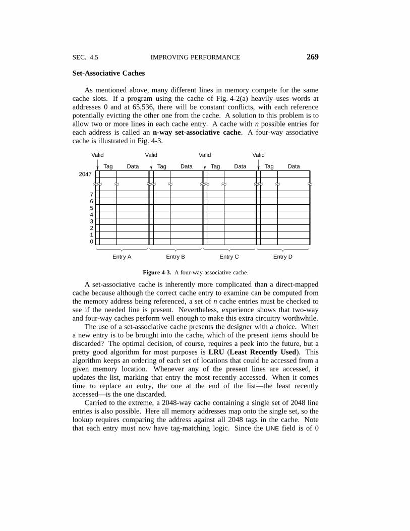
SEC. 4.5 IMPROVING PERFORMANCE 269
Set-Associative Caches
As mentioned above, many different lines in memory compete for the samecache slots. If a program using the cache of Fig. 4-2(a) heavily uses words ataddresses 0 and at 65,536, there will be constant conflicts, with each referencepotentially evicting the other one from the cache. A solution to this problem is toallow two or more lines in each cache entry. A cache with n possible entries foreach address is called an n-way set-associative cache. A four-way associativecache is illustrated in Fig. 4-3.
Valid
Tag Data2047
76543210
Entry A
Valid
Tag Data
Entry B
Valid
Tag Data
Entry C
Valid
Tag Data
Entry D
Figure 4-3. A four-way associative cache.
A set-associative cache is inherently more complicated than a direct-mappedcache because although the correct cache entry to examine can be computed fromthe memory address being referenced, a set of n cache entries must be checked tosee if the needed line is present. Nevertheless, experience shows that two-wayand four-way caches perform well enough to make this extra circuitry worthwhile.
The use of a set-associative cache presents the designer with a choice. Whena new entry is to be brought into the cache, which of the present items should bediscarded? The optimal decision, of course, requires a peek into the future, but apretty good algorithm for most purposes is LRU (Least Recently Used). Thisalgorithm keeps an ordering of each set of locations that could be accessed from agiven memory location. Whenever any of the present lines are accessed, itupdates the list, marking that entry the most recently accessed. When it comestime to replace an entry, the one at the end of the list—the least recentlyaccessed—is the one discarded.
Carried to the extreme, a 2048-way cache containing a single set of 2048 lineentries is also possible. Here all memory addresses map onto the single set, so thelookup requires comparing the address against all 2048 tags in the cache. Notethat each entry must now have tag-matching logic. Since the LINE field is of 0

270 THE MICROARCHITECTURE LEVEL CHAP. 4
length, the TAG field is the entire address except for the WORD and BYTE fields.Furthermore, when a cache line is replaced, all 2048 locations are possible candi-dates for replacement. Maintaining an ordered list of 2048 entries requires a greatdeal of bookkeeping, making LRU replacement infeasible. (Remember that thislist has to be updated on every memory operation, not just on a miss). Surpris-ingly, high-associativity caches do not improve performance much over low-associativity caches under most circumstances, and in some cases actually per-form worse. For these reasons, associativity beyond four-way is quite unusual.
Finally, writes pose a special problem for caches. When a processor writes aword, and the word is in the cache, it obviously must either update the word ordiscard the cache entry. Nearly all designs update the cache. But what aboutupdating the copy in main memory? This operation can be deferred until later,when the cache line is ready to be replaced by the LRU algorithm. This choice isdifficult, and neither option is clearly preferable. Immediately updating the entryin main memory is referred to as write through. This approach is generallysimpler to implement and more reliable, since the memory is always up to date—helpful, for example, if an error occurs and it is necessary to recover the state ofthe memory. Unfortunately, it also usually requires more write traffic to memory,so more sophisticated implementations tend to employ the alternative, known aswrite deferred, or write back.
A related problem must be addressed for writes: what if a write occurs to alocation that is not currently cached? Should the data be brought into the cache,or just written out to memory? Again, neither answer is always best. Mostdesigns that defer writes to memory tend to bring data into the cache on a writemiss, a technique known as write allocation. Most designs employing writethrough, on the other hand, tend not to allocate an entry on a write because thisoption complicates an otherwise simple design. Write allocation wins only ifthere are repeated writes to the same or different words within a cache line.
4.5.2 Branch Prediction
Modern computers are highly pipelined. The pipeline of Fig. 4-0 has sevenstages; high-end computers sometimes have 10-stage pipelines or even more.Pipelining works best on linear code, so the fetch unit can just read in consecutivewords from memory and send them off to the decode unit in advance of theirbeing needed.
The only minor problem with this wonderful model is that it is not the slight-est bit realistic. Programs are not linear code sequences. They are full of branchinstructions. Consider the simple statements of Fig. 4-4(a). A variable, i, is com-pared to 0 (probably the most common test in practice). Depending on the result,another variable, k, gets assigned one of two possible values.
A possible translation to assembly language is shown in Fig. 4-4(b). We willstudy assembly language later in this book, and the details are not important now,

SEC. 4.5 IMPROVING PERFORMANCE 271
if (i == 0) CMP i,0 ; compare i to 0k = 1; BNE Else ; branch to Else if not equal
else Then: MOV k,1 ; move 1 to kk = 2; BR Next ; unconditional branch to Next
Else: MOV k,2 ; move 2 to kNext:
(a) (b)
Figure 4-4. (a) A program fragment. (b) Its translation to a generic assemblylanguage.
but depending on the machine and the compiler, code more-or-less like that ofFig. 4-4(b) is likely. The first instruction compares i to 0. The second onebranches to the label Else (the start of the else clause) if i is not 0. The thirdinstruction assigns 1 to k. The fourth instruction branches to the code for the nextstatement. The compiler has conveniently planted a label, Next, there, so there isa place to branch to. The fifth instruction assigns 2 to k.
The thing to observe here is that two of the five instructions are branches.Furthermore, one of these, BNE, is a conditional branch (a branch that is taken ifand only if some condition is met, in this case, that the two operands in the previ-ous CMP are equal). The longest linear code sequence here is two instructions.As a consequence, fetching instructions at a high rate to feed the pipeline is verydifficult.
At first glance, it might appear that unconditional branches, such as theinstruction BR Next in Fig. 4-4(b), are not a problem. After all, there is no ambi-guity about where to go. Why can’t the fetch unit just continue to read instruc-tions from the target address (the place that will be branched to)?
The trouble lies in the nature of pipelining. In Fig. 4-0, for example, we seethat instruction decoding occurs in the second stage. Thus the fetch unit has todecide where to fetch from next before it knows what kind of instruction it justgot. Only one cycle later can it learn that it just picked up an unconditionalbranch, and by then it has already started to fetch the instruction following theunconditional branch. As a consequence, a substantial number of pipelinedmachines (such as the UltraSPARC II) have the property that the instruction fol-lowing an unconditional branch is executed, even though logically it should notbe. The position after a branch is called a delay slot. The Pentium II [and themachine used in Fig. 4-4(b)] do not have this property, but the internal complexityto get around this problem is often enormous. An optimizing compiler will try tofind some useful instruction to put in the delay slot, but frequently there is nothingavailable, so it is forced to insert a NOP instruction there. Doing so keeps the pro-gram correct, but makes it bigger and slower.
Annoying as unconditional branches are, conditional branches are worse. Notonly do they also have delay slots, but now the fetch unit does not where to read

272 THE MICROARCHITECTURE LEVEL CHAP. 4
from until much later in the pipeline. Early pipelined machines just stalled until itwas known whether the branch would be taken or not. Stalling for three or fourcycles on every conditional branch, especially if 20% of the instructions are con-ditional branches, wreaks havoc with the performance.
Consequently, what most machines do when they hit a conditional branch ispredict whether it is going to be taken or not. It would be nice if we could justplug a crystal ball into a free PCI slot to help out with the prediction, but so farthis approach has not borne fruit.
Lacking such a peripheral, various ways have been devised to do the predic-tion. One very simple way is as follows: assume that all backward conditionalbranches will be taken and that all forward ones will not be taken. The reasoningbehind the first part is that backward branches are frequently located at the end ofa loop. Most loops are executed multiple times, so guessing that a branch back tothe top of the loop will be taken is generally a good bet.
The second part is shakier. Some forward branches occur when error condi-tions are detected in software (e.g., a file cannot be opened). Errors are rare, somost of the branches associated with them are not taken. Of course, there areplenty of forward branches not related to error handling, so the success rate is notnearly as good as with backward branches. While not fantastic, this rule is at leastbetter than nothing.
If a branch is correctly predicted, there is nothing special to do. Executionjust continues at the target address. The trouble comes when a branch is predictedwrongly. Figuring out where to go and going there is not difficult. The hard partis undoing instructions that have already been executed and should not have been.
There are two ways of going about this. The first way is to allow instructionsfetched after a predicted conditional branch to execute until they try to change themachine’s state (e.g., storing into a register). Instead of overwriting the register,the value computed is put into a (secret) scratch register and only copied to thereal register after it is known that the prediction was correct. The second way isto record the value of any register about to be overwritten (e.g., in a secret scratchregister), so the machine can be rolled back to the state it had at the time of themispredicted branch. Both solutions are complex and require industrial-strengthbookkeeping to get them right. And if a second conditional branch is hit before itis known whether the first one was predicted right, things can get really messy.
Dynamic Branch Prediction
Clearly, having the predictions be accurate is of great value, since it allowsthe CPU to proceed at full speed. As a consequence, a great deal of currentresearch aims at improving branch prediction algorithms (e.g., Driesen and Hol-zle, 1998; Juan et al., 1998; Pan et al., 1992; Sechrest et al., 1996; Sprangle et al.,1997; and Yeh and Patt, 1991). One approach is for the CPU to maintain a historytable (in special hardware), in which it logs conditional branches as they occur, so

SEC. 4.5 IMPROVING PERFORMANCE 273
they can be looked up when they occur again. The simplest version of thisscheme is shown in Fig. 4-5(a). Here the history table contains one entry for eachconditional branch instruction. The entry contains the address of the branchinstruction along with a bit telling whether it was taken the last time it was exe-cuted. Using this scheme, the prediction is simply that the branch will go thesame way it went last time. If the prediction is wrong, the bit in the history tableis changed.
Valid
6543210
Branch/no branch
SlotBranchaddress/tag
Targetaddress
(a)
Valid
6543210
Predictionbits
SlotBranchaddress/tag
(c)
Valid
6543210
PredictionbitsSlot
Branchaddress/tag
(b)
Figure 4-5. (a) A 1-bit branch history. (b) A 2-bit branch history. (c) A map-ping between branch instruction address and target address.
There are several ways to organize the history table. In fact, these are pre-cisely the same ways used to organize a cache. Consider a machine with 32-bitinstructions that are word aligned so that the low-order 2 bits of each memoryaddress are 00. With a direct-mapped history table containing 2n entries, thelow-order n + 2 bits of a branch instruction can be extracted and shifted right 2bits. This n-bit number can be used as an index into the history table where acheck is made to see if the address stored there matches the address of the branch.As with a cache, there is no need to store the low-order n + 2 bits, so they can beomitted (i.e., just the upper address bits—the tag—are stored). If there is a hit, theprediction bit is used to predict the branch. If the wrong tag is present or the entryis invalid, a miss occurs, just as with a cache. In this case, the forward/backwardbranch rule can be used.
If the branch history table has, say, 4096 entries, then branches at addresses 0,16384, 32768, ... will conflict, analogous to the same problem with a cache. Thesame solution is possible: a two-way, four-way, or n-way associative entry. Aswith a cache, the limiting case is a single n-way associative entry, which requiresfull associativity of lookup.
Given a large enough table size and enough associativity, this scheme workswell in most situations. However, one systematic problem always occurs. Whena loop is finally exited, the branch at the end will be mispredicted, and worse yet,the misprediction will change the bit in the history table to indicate a future pred-iction of ‘‘no branch.’’ The next time the loop is entered, the branch at the end of

274 THE MICROARCHITECTURE LEVEL CHAP. 4
the first iteration will be predicted wrong. If the loop is inside an outer loop, or ina frequently-called procedure, this error can occur often.
To eliminate this misprediction, we can give the table entry a second chance.With this method, the prediction is only changed after two consecutive incorrectpredictions. This approach requires having two prediction bits in the history table,one for what the branch is ‘‘supposed’’ to do, and one for what it did last time, asshown in Fig. 4-5(b).
A slightly different way of looking at this algorithm is to see it as a finite-statemachine with four states, as depicted in Fig. 4-6. After a series of consecutivesuccessful ‘‘no branch’’ predictions, the FSM will be in state 00 and will predict‘‘no branch’’ next time. If that prediction is wrong, it will move to state 10, butpredict ‘‘no branch’’ next time as well. Only if this prediction is wrong will itnow move to state 11 and predict branches all the time. In effect, the leftmost bitof the state is the prediction and the rightmost bit is what the branch did last time.While this design uses only 2 bits of history, a design that keeps track of 4 or 8bits of history is also possible.
No branch
Branch
Branch
00
Nobranch
Predictno branch
01
Predictno branchone more
time
10
Predictbranch
one moretime
Branch
Nobranch
Branch
No branch
11
Predictbranch
Figure 4-6. A 2-bit finite-state machine for branch prediction.
This is not our first FSM. Fig. 4-0 was also an FSM. In fact, all of ourmicroprograms can be regarded as FSMs, since each line represents a specificstate the machine can be in, with well-defined transitions to a finite set of otherstates. FSMs are very widely used in all aspects of hardware design.
So far, we have assumed that the target of each conditional branch wasknown, typically either as an explicit address to branch to (contained within theinstruction itself), or as a relative offset from the current instruction (i.e., a signednumber to add to the program counter). Often this assumption is valid, but someconditional branch instructions compute the target address by doing arithmetic onregisters, and then going there. Even if the FSM of Fig. 4-6 accurately predictsthe branch will be taken, such a prediction is of no use if the target address isunknown. One way of dealing with this situation is to store the actual address

SEC. 4.5 IMPROVING PERFORMANCE 275
branched to last time in the history table, as shown in Fig. 4-5(c). In this way, ifthe table says that the last time the branch at address 516 was taken it went toaddress 4000, if the prediction is now for ‘‘branch,’’ the working assumption willbe a branch to 4000 again.
A different approach to branch prediction is to keep track of whether the last kconditional branches encountered were taken, irrespective of which instructionsthey were (Pan et al., 1992). This k-bit number, kept in the branch history shiftregister, is then compared in parallel to all the entries of a history table with a k-bit key and if a hit occurs, the prediction found there used. Somewhat surpris-ingly, this technique works quite well.
Static Branch Prediction
All of the branch prediction techniques discussed so far are dynamic, that is,carried out at run time while the program is running. They also adapt to theprogram’s current behavior, which is good. The down side is that they requirespecialized and expensive hardware and a great deal of chip complexity.
A different way to go is to have the compiler help out. When the compilersees a statement like
for (i = 0; i < 1000000; i++) { ... }
it knows very well that the branch at the end of the loop will be taken nearly allthe time. If only there were a way for it to tell the hardware, a lot of effort couldbe saved.
Although this is an architectural change (and not just an implementationissue), some machines, such as the UltraSPARC II, have a second set of condi-tional branch instructions, in addition to the regular ones (which are needed forbackward compatibility). The new ones contain a bit in which the compiler canspecify that it thinks the branch will be taken (or not taken). When one of these isencountered, the fetch unit just does what it has been told. Furthermore, there isno need to waste precious space in the branch history table for these instructions,thus reducing conflicts there.
Finally, our last branch prediction technique is based on profiling (Fisher andFreudenberger, 1992). This, too, is a static technique, but instead of having thecompiler try to figure out which branches will be taken and which will not, theprogram is actually run (typically on a simulator), and the branch behavior cap-tured. This information is fed into the compiler, which then uses the special con-ditional branch instructions to tell the hardware what to do.

276 THE MICROARCHITECTURE LEVEL CHAP. 4
4.5.3 Out-of-Order Execution and Register Renaming
Most modern CPUs are both pipelined and superscalar, as shown in Fig. 2-6.What this generally means is that there is a fetch unit that pulls instruction wordsout of memory before they are needed in order to feed a decode unit. The decodeunit issues the decoded instructions to the proper functional units for execution.In some cases it may break individual instructions into micro-ops before issuingthem to the functional units, depending on what the functional units are capable ofdoing.
Clearly, the machine design is simplest if all instructions are executed in theorder they are fetched (assuming for the moment that the branch prediction algo-rithm never guesses wrong). However, in-order execution does not always giveoptimal performance due to dependences between instructions. If an instructionneeds a value computed by the previous instruction, the second one cannot beginexecuting until the first one has produced the needed value. In this situation (aRAW dependence), the second instruction has to wait. Other kinds of depen-dences also exist, as we will soon see.
In an attempt to get around these problems and produce better performance,some CPUs allow dependent instructions to be skipped over, to get to futureinstructions that are not dependent. Needless to say, the internal instructionscheduling algorithm used must deliver the same effect as if the program wereexecuted in the order written. We will now demonstrate how instruction reorder-ing works using a detailed example.
To illustrate the nature of the problem, we will start with a machine thatalways issues instructions in program order and also requires them to completeexecution in program order. The significance of the latter point will become clearlater.
Our example machine has eight registers visible to the programmer, R0through R7. All arithmetic instructions use three registers: two for the operandsand one for the result, the same as the Mic-4. We will assume that if an instruc-tion is decoded in cycle n, execution starts in cycle n + 1. For a simple instruc-tion, such as an addition or subtraction, the writeback to the destination registeroccurs at the end of cycle n + 2. For a more complicated instruction, such as amultiplication, the writeback occurs at the end of cycle n + 3. To make the exam-ple realistic, we will allow the decode unit to issue up to two instructions perclock cycle. Commercial superscalar CPUs often can issue four or even sixinstructions per clock cycle.
Our example execution sequence is shown in Fig. 4-7. Here the first columngives the number of the cycle and the second one gives the instruction number.The third column lists the instruction decoded. The fourth one tells which instruc-tion is being issued (with a maximum of two per clock cycle). The fifth one tellswhich instruction has been retired (completed). Remember that in this examplewe are requiring both in-order issue and in-order completion, so instruction k + 1

SEC. 4.5 IMPROVING PERFORMANCE 277
cannot be issued until instruction k has been issued, and instruction k + 1 cannotbe retired (meaning the writeback to the destination register is performed) untilinstruction k has been retired. The other 16 columns are discussed below.222222222222222222222222222222222222222222222222222222222222222222222222222222222
Registers being read Registers being written222222222222222222222222222222222222222222222222222222222222222222222222222222222Cy # Decoded Iss Ret 0 1 2 3 4 5 6 7 0 1 2 3 4 5 6 7222222222222222222222222222222222222222222222222222222222222222222222222222222222
1 1 R3=R0*R1 1 1 1 12 R4=R0+R2 2 2 1 1 1 1222222222222222222222222222222222222222222222222222222222222222222222222222222222
2 3 R5=R0+R1 3 3 2 1 1 1 14 R6=R1+R4 – 3 2 1 1 1 1222222222222222222222222222222222222222222222222222222222222222222222222222222222
3 3 2 1 1 1 12222222222222222222222222222222222222222222222222222222222222222222222222222222224 1 2 1 1 1 1
2 1 1 13222222222222222222222222222222222222222222222222222222222222222222222222222222222
5 4 1 1 15 R7=R1*R2 5 2 1 1 1 1222222222222222222222222222222222222222222222222222222222222222222222222222222222
6 6 R1=R0−R2 – 2 1 1 1 12222222222222222222222222222222222222222222222222222222222222222222222222222222227 4 1 1 12222222222222222222222222222222222222222222222222222222222222222222222222222222228 52222222222222222222222222222222222222222222222222222222222222222222222222222222229 6 1 1 1
7 R3=R3*R1 7 1 1 1 1 1 122222222222222222222222222222222222222222222222222222222222222222222222222222222210 1 1 1 1 1 122222222222222222222222222222222222222222222222222222222222222222222222222222222211 6 1 1 122222222222222222222222222222222222222222222222222222222222222222222222222222222212 722222222222222222222222222222222222222222222222222222222222222222222222222222222213 8 R1=R4+R4 8 2 122222222222222222222222222222222222222222222222222222222222222222222222222222222214 2 122222222222222222222222222222222222222222222222222222222222222222222222222222222215 822222222222222222222222222222222222222222222222222222222222222222222222222222222211111111111111111111111111111111111
111111111111111111111111111111111
111111111111111111111111111111111
111111111111111111111111111111111
111111111111111111111111111111111
11111111111111111111111111111111111
11111111111111111111111111111111111
111111111111111111111111111111111
111111111111111111111111111111111
111111111111111111111111111111111
111111111111111111111111111111111
111111111111111111111111111111111
111111111111111111111111111111111
111111111111111111111111111111111
11111111111111111111111111111111111
11111111111111111111111111111111111
111111111111111111111111111111111
111111111111111111111111111111111
111111111111111111111111111111111
111111111111111111111111111111111
111111111111111111111111111111111
111111111111111111111111111111111
111111111111111111111111111111111
11111111111111111111111111111111111
Figure 4-7. Operation of a superscalar CPU with in-order issue and in-ordercompletion.
After decoding an instruction, the decode unit has to decide whether or not itcan be issued immediately. To make this decision, the decode unit needs to knowthe status of all the registers. If, for example, the current instruction needs a regis-ter whose value has not yet been computed, the current instruction cannot beissued and the CPU must stall.
We will keep track of register use with a device called a scoreboard, whichwas first present in the CDC 6600. The scoreboard has a small counter for eachregister telling how many times that register is in use as a source by currently-executing instructions. If a maximum of, say, 15 instructions may be executing atonce, then a 4-bit counter will do. When an instruction is issued, the scoreboardentries for its operand registers are incremented. When an instruction is retired,

278 THE MICROARCHITECTURE LEVEL CHAP. 4
the entries are decremented.The scoreboard also has a counter for each register to keep track of registers
being used as destinations. Since only one write at a time is allowed, thesecounters can be 1-bit wide. The rightmost 16 columns in Fig. 4-7 show the score-board.
In real machines, the scoreboard also keeps track of functional unit usage, toavoid issuing an instruction for which no functional unit is available. For simpli-city, we will assume there is always a suitable functional unit available, so wewill not show the functional units on the scoreboard.
The first line of Fig. 4-7 shows I1 (instruction 1), which multiplies R0 by R1and puts the result in R3. Since none of these registers are in use yet, the instruc-tion is issued and the scoreboard is updated to reflect that R0 and R1 are beingread and R3 is being written. No subsequent instruction can write into any ofthese or can read R3 until I1 has been retired. Since this instruction is a multipli-cation, it will be finished at the end of cycle 4. The scoreboard values shown oneach line reflect their state after the instruction on that line has been issued.Blank entries are 0s.
Since our example is a superscalar machine that can issue two instructions percycle, a second instruction (I2) is issued during cycle 1. It adds R0 and R2, storingthe result in R4. To see if this instruction can be issued, the following rules areapplied:
1. If any operand is being written, do not issue (RAW dependence).
2. If the result register is being read, do not issue (WAR dependence).
3. If the result register is being written, do not issue (WAW dependence).
We have already seen RAW dependences, which occur when an instruction needsto use as a source a result that a previous instruction has not yet produced. Theother two dependences are less serious. They are essentially resource conflicts.In a WAR dependence (Write After Read), one instruction is trying to overwritea register that a previous instruction may not yet have finished reading. A WAWdependence (Write After Write) is similar. These can often be avoided by havingthe second instruction put its results somewhere else (perhaps temporarily). Ifnone of the above three dependences exist, and the functional unit it needs isavailable, the instruction is issued. In this case, I2 uses a register (R0) that isbeing read by a pending instruction, but this overlap is permitted so I2 is issued.Similarly, I3 is issued during cycle 2.
Now we come to I4, which needs to use R4. Unfortunately, we see from line3 that R4 is being written. Here we have a RAW dependence, so the decode unitstalls until R4 becomes available. While stalled, it stops pulling instructions fromthe fetch unit. When the fetch unit’s internal buffers fill up, it will stop prefetch-ing.
It is worth noting that the next instruction in program order, I5, does not have

SEC. 4.5 IMPROVING PERFORMANCE 279
conflicts with any of the pending instructions. It could have been decoded andissued were it not for the fact that this design requires issuing instructions inorder.
Now let us look at what happens during cycle 3. I2, being an addition (twocycles), finishes at the end of cycle 3. Unfortunately, it cannot be retired (thusfreeing up R4 for I4). Why not? The reason is that this design also requires in-order retirement. Why? What harm could possibly come from doing the storeinto R4 now and marking it as available?
The answer is subtle, but important. Suppose that instructions could completeout of order. Then if an interrupt occurred, it would be very difficult to save thestate of the machine so it could be restored later. In particular, it would not bepossible to say that all instructions up to some address had been executed and allinstructions beyond it had not. This is called a precise interrupt and is a desir-able characteristic in a CPU (Moudgill and Vassiliadis, 1996). Out-of-orderretirement makes interrupts imprecise, which is why some machines require in-order instruction completion.
Getting back to our example, at the end of cycle 4, all three pending instruc-tions can be retired, so in cycle 5 I4 can finally be issued, along with the newlydecoded I5. Whenever an instruction is retired, the decode unit has to check tosee if there is a stalled instruction that can now be issued.
In cycle 6, I6 stalls because it needs to write into R1 and R1 is busy. It isfinally started in cycle 9. The entire sequence of eight instructions takes 15 cyclesto complete due to many dependences, even though the hardware is capable ofissuing two instructions on every cycle. Notice, however, that when readingdown the Iss column of Fig. 4-7, all the instructions have been issued in order.Likewise, the Ret column shows that they have been retired in order as well.
Now let us consider an alternative design: out-of-order execution. In thisdesign, instructions may be issued out of order and may be retired out of order aswell. The same sequence of eight instructions is shown in Fig. 4-8, only now without-of-order issue and out-of-order retirement permitted.
The first difference occurs in cycle 3. Even though I4 has stalled, we candecode and issue I5 since it does not conflict with any pending instruction. How-ever, skipping over instructions causes a new problem. Suppose that I5 had usedan operand computed by the skipped instruction, I4. With the current scoreboard,we would not have noticed this. As a consequence, we have to extend the score-board to keep track of stores done by skipped-over instructions. This can be doneby adding a second bit map, 1 bit per register, to keep track of stores done bystalled instructions. (These counters are not shown in the figure.) The rule forissuing instructions now has to be extended to prevent the issue of any instructionwith an operand scheduled to be stored into by an instruction that came before itbut was skipped over.
Now let us look back at I6, I7, and I8 in Fig. 4-7. Here we see that I6 com-putes a value in R1 that is used by I7. However, we also see that the value is
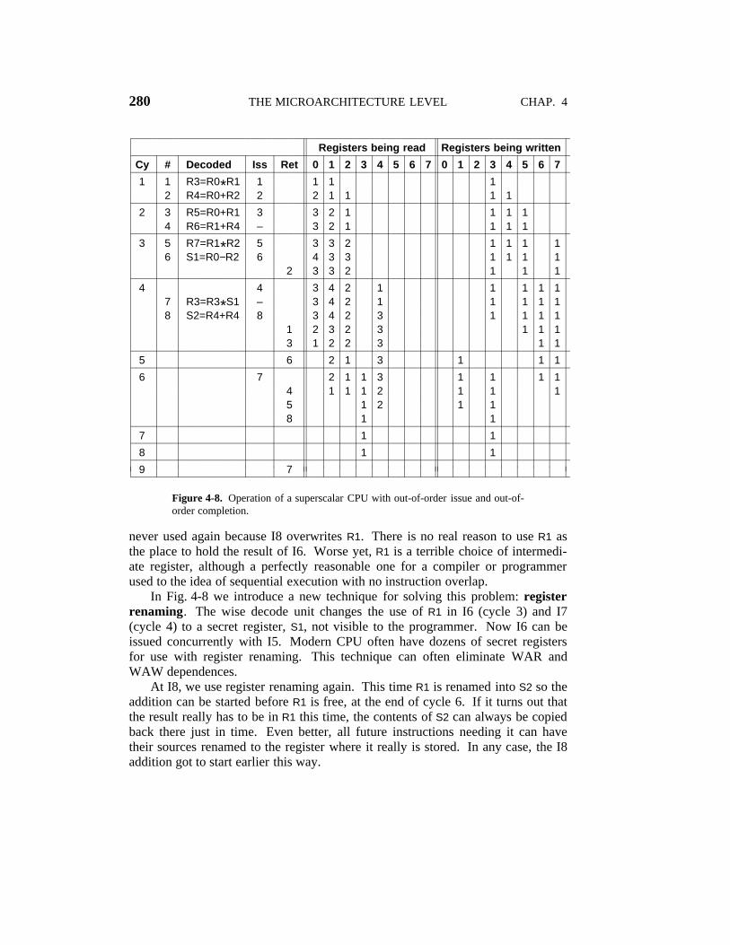
280 THE MICROARCHITECTURE LEVEL CHAP. 4
222222222222222222222222222222222222222222222222222222222222222222222222222222222Registers being read Registers being written222222222222222222222222222222222222222222222222222222222222222222222222222222222
Cy # Decoded Iss Ret 0 1 2 3 4 5 6 7 0 1 2 3 4 5 6 72222222222222222222222222222222222222222222222222222222222222222222222222222222221 1 R3=R0*R1 1 1 1 1
2 R4=R0+R2 2 2 1 1 1 12222222222222222222222222222222222222222222222222222222222222222222222222222222222 3 R5=R0+R1 3 3 2 1 1 1 1
4 R6=R1+R4 – 3 2 1 1 1 12222222222222222222222222222222222222222222222222222222222222222222222222222222223 5 R7=R1*R2 5 3 3 2 1 1 1 1
6 S1=R0−R2 6 4 3 3 1 1 1 12 3 3 2 1 1 1222222222222222222222222222222222222222222222222222222222222222222222222222222222
4 4 3 4 2 1 1 1 1 17 R3=R3*S1 – 3 4 2 1 1 1 1 18 S2=R4+R4 8 3 4 2 3 1 1 1 1
1 2 3 2 3 1 1 13 1 2 2 3 1 1222222222222222222222222222222222222222222222222222222222222222222222222222222222
5 6 2 1 3 1 1 12222222222222222222222222222222222222222222222222222222222222222222222222222222226 7 2 1 1 3 1 1 1 1
4 1 1 1 2 1 1 15 1 2 1 18 1 1222222222222222222222222222222222222222222222222222222222222222222222222222222222
7 1 12222222222222222222222222222222222222222222222222222222222222222222222222222222228 1 12222222222222222222222222222222222222222222222222222222222222222222222222222222229 722222222222222222222222222222222222222222222222222222222222222222222222222222222211
111111111111111111111111111111
111111111111111111111111111111
111111111111111111111111111111
111111111111111111111111111111
111111111111111111111111111111
11111111111111111111111111111111
11111111111111111111111111111111
111111111111111111111111111111
111111111111111111111111111111
111111111111111111111111111111
111111111111111111111111111111
111111111111111111111111111111
111111111111111111111111111111
111111111111111111111111111111
11111111111111111111111111111111
11111111111111111111111111111111
111111111111111111111111111111
111111111111111111111111111111
111111111111111111111111111111
111111111111111111111111111111
111111111111111111111111111111
111111111111111111111111111111
111111111111111111111111111111
11111111111111111111111111111111
Figure 4-8. Operation of a superscalar CPU with out-of-order issue and out-of-order completion.
never used again because I8 overwrites R1. There is no real reason to use R1 asthe place to hold the result of I6. Worse yet, R1 is a terrible choice of intermedi-ate register, although a perfectly reasonable one for a compiler or programmerused to the idea of sequential execution with no instruction overlap.
In Fig. 4-8 we introduce a new technique for solving this problem: registerrenaming. The wise decode unit changes the use of R1 in I6 (cycle 3) and I7(cycle 4) to a secret register, S1, not visible to the programmer. Now I6 can beissued concurrently with I5. Modern CPU often have dozens of secret registersfor use with register renaming. This technique can often eliminate WAR andWAW dependences.
At I8, we use register renaming again. This time R1 is renamed into S2 so theaddition can be started before R1 is free, at the end of cycle 6. If it turns out thatthe result really has to be in R1 this time, the contents of S2 can always be copiedback there just in time. Even better, all future instructions needing it can havetheir sources renamed to the register where it really is stored. In any case, the I8addition got to start earlier this way.

SEC. 4.5 IMPROVING PERFORMANCE 281
On many real machines, renaming is deeply embedded in the way the regis-ters are organized. There are many secret registers and a table that maps theregisters visible to the programmer onto the secret registers. Thus the real registerbeing used for, say, R0 is located by looking at entry 0 of this mapping table. Inthis way, there is no real register R0, just a binding between the name R0 and oneof the secret registers. This binding changes frequently during execution to avoiddependences.
Notice that in Fig. 4-8 when reading down the fourth column, the instructionshave not been issued in order. Nor they have been retired in order. The conclu-sion of this example is simple: using out-of-order execution and register renamingwe were able to speed up the computation by close to a factor of two.
4.5.4 Speculative Execution
In the previous section we introduced the concept of reordering instructions inorder to improve performance. Although we did not mention it explicitly, thefocus there was on reordering instructions within a single basic block. It is nowtime to look at this point more closely.
Computer programs can be broken up into basic blocks, with each basicblock consisting of a linear sequence of code with one entry point on top and oneexit on the bottom. A basic block does not contain any control structures (e.g., ifstatements or while statements) so that its translation into machine language doesnot contain any branches. The basic blocks are connected by control statements.
A program in this form can be represented as a directed graph, as shown inFig. 4-9. Here we compute the sum of the cubes of the even and odd integers upto some limit and accumulate them in evensum and oddsum, respectively. Withineach basic block, the reordering techniques of the previous section work fine.
The trouble is that most basic blocks are short and there is insufficient paral-lelism in them to exploit effectively. Consequently, the next step is to allow thereordering to cross basic block boundaries in an attempt to fill all the issue slots.The biggest gains come when a potentially slow operation can be moved upwardin the graph to start it going early. This might be a LOAD instruction, a floating-point operation, or even the start of a long dependence chain. Moving codeupward over a branch is called hoisting.
Imagine that in Fig. 4-9 all the variables were kept in registers except even-sum and oddsum (for lack of registers). It might make sense then to move theirLOAD instructions to the top of the loop, before computing k, to get them startedearly on, so the values will available when they are needed. Of course, only oneof them will be needed on each iteration, so the other LOAD will be wasted, but ifthe cache and memory are pipelined and there are issue slots available, it mightstill be worth doing this. Executing code before it is known if it is even going tobe needed is called speculative execution. Using this technique requires supportfrom the compiler and the hardware as well as some architectural extensions. In

282 THE MICROARCHITECTURE LEVEL CHAP. 4
evensum = 0;
oddsum = 0;
i = 0;
while (i < limit) {
k = i * i * i;k = i * i * i;
if ((i/2) * 2) == 0)
evensum = evensum + k;
else
oddsum = oddsum + k;
}(a) (b)
evensum = 0;
oddsum = 0;
i = 0;
while (i < limit)
if ((i/2) * 2) = = 0)
T F
evensum = evensum + k; oddsum = oddsum + k;
i = i + 1;i = i + 1;
i >= limit
Figure 4-9. (a) A program fragment. (b) The corresponding basic block graph.
most cases, reordering instructions over basic block boundaries is beyond thecapability of the hardware, so the compiler must move the instructions explicitly.
Speculative execution introduces some interesting problems. For one, it isessential that none of the speculative instructions have irrevocable results becauseit may turn out later that they should not have been executed. In Fig. 4-9, it is fineto fetch evensum and oddsum, and it is also fine to do the addition as soon as k isavailable (even before the if statement), but it is not fine to store the results backin memory. In more complicated code sequences, one common way of preventingspeculative code from overwriting registers before it is known if this is desired isto rename all the destination registers used by the speculative code. In this way,only scratch registers are modified, so there is no problem if the code ultimately isnot needed. If the code is needed, the scratch registers are copied to the true des-tination registers. As you can imagine, the scoreboarding to keep track of all thisis not simple, but given enough hardware, it can be done.
However, there is another problem introduced by speculative code that cannotbe solved by register renaming. What happens if a speculatively executed instruc-tion causes an exception? A painful, but not fatal, example is a LOAD instructionthat causes a cache miss on a machine with a large cache line size (say, 256 bytes)and a memory far slower than the CPU and cache. If a LOAD that is actuallyneeded stops the machine dead in its tracks for many cycles while the cache lineis being loaded, well, that’s life, since the word is needed. However, stalling themachine to fetch a word that turns out not to be needed is counterproductive. Toomany of these ‘‘optimizations,’’ may make the CPU slower than if it did not havethem at all. (If the machine has virtual memory, which is discussed in Chap. 6, a

SEC. 4.5 IMPROVING PERFORMANCE 283
speculative LOAD might even cause a page fault, which requires a disk operationto bring in the needed page. False page faults can have a terrible effect on perfor-mance, so it is important to avoid them.)
One solution present in a number of modern machines is to have a specialSPECULATIVE-LOAD instruction that tries to fetch the word from the cache, but ifit is not there, just gives up. If the value is there when it is actually needed, it canbe used, but if it is not, the hardware must go out and get it on the spot. If thevalue turns out not to be needed, no penalty has been paid for the cache miss.
A far worse situation can be illustrated with the following statement:
if (x > 0) z = y/x;
where x, y, and z are floating-point variables. Suppose that the variables are allfetched into registers in advance and that the (slow) floating-point division ishoisted above the if test. Unfortunately, x is 0 and the resulting divide-by-zerotrap terminates the program. The net result is that speculation has caused acorrect program to fail. Worse yet, the programmer put in explicit code to preventthis situation and it happened anyway. This situation is not likely to lead to ahappy programmer.
One possible solution is to have special versions of instructions that mightcause exceptions. In addition, a bit, called a poison bit, is added to each register.When a special speculative instruction fails, instead of causing a trap, it sets thepoison bit on the result register. If that register is later touched by a regularinstruction, the trap occurs then (as it should). However, if the result is neverused, the poison bit is eventually cleared and no harm is done.

5THE INSTRUCTION SET
ARCHITECTURE LEVEL
1

Software
Hardware
Hardware
C program
ISA level
ISA program executedby microprogram or hardware
FORTRAN 90program
FORTRAN 90program compiledto ISA program
C programcompiledto ISA program
Figure 5-1. The ISA level is the interface between the com-pilers and the hardware.
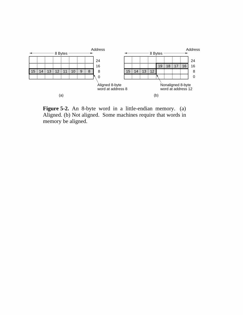
24
Address
Aligned 8-byteword at address 8
16815 14 13 12 11
(a)
10 9 8
0
8 Bytes
24
Address
Nonaligned 8-byteword at address 12
16815 14 13 12
19
(b)
18 17 16
0
8 Bytes
Figure 5-2. An 8-byte word in a little-endian memory. (a)Aligned. (b) Not aligned. Some machines require that words inmemory be aligned.

EAXALAHA X
EBXBLBHB X
ECXCLCHC X
EDX
ESI
EDI
EBP
ESP
DL
CS
EIP
EFLAGS
SS
DS
ES
FS
GS
DHD X
8816Bits
Figure 5-3. The Pentium II’s primary registers.

222222222222222222222222222222222222222222222222222222222222222222222Register Alt. name Function222222222222222222222222222222222222222222222222222222222222222222222
R0 G0 Hardwired to 0. Stores into it are just ignored.222222222222222222222222222222222222222222222222222222222222222222222R1 – R7 G1 – G7 Holds global variables222222222222222222222222222222222222222222222222222222222222222222222R8 – R13 O0 – O5 Holds parameters to the procedure being called222222222222222222222222222222222222222222222222222222222222222222222R14 SP Stack pointer222222222222222222222222222222222222222222222222222222222222222222222R15 O7 Scratch register222222222222222222222222222222222222222222222222222222222222222222222R16 – R23 L0 – L7 Holds local variables for the current procedure222222222222222222222222222222222222222222222222222222222222222222222R24 – R29 I0 – I5 Holds incoming parameters222222222222222222222222222222222222222222222222222222222222222222222R30 FP Pointer to the base of the current stack frame222222222222222222222222222222222222222222222222222222222222222222222R31 I7 Holds return address for the current procedure222222222222222222222222222222222222222222222222222222222222222222222111111111111111
111111111111111
111111111111111
111111111111111
Figure 5-4. The UltraSPARC II’s general registers.

R0R1
G0G1
0Global 1
R13R14R15
OSSPO7
Outgoing parmeter 5Stack pointerTemporary
R8 O0 Outgoing parmeter 0
R29R30R31
I5FPI7
Incoming parmeter 5Frame pointerReturn address
R24 10 Incoming parameter 0
R29R30R31
I5FPI7
Incoming parmeter 5Frame pointerReturn address
R24 I0 Incoming parameter 0
R16 L0 Local 0
R7 G7 Global 7
(a)
R23 L7 Local 7
R16 L0 Local 0
R23 L7 Local 7
R13R14R15
O5SPO7
Stack pointerTemporary
R8 O0
Alternative name
R0R1
G0G1
0Global 1
CWPdecremented
on call inthis direction
Overlap
CWP = 7
CWP = 6
Part ofprevious window
Part ofprevious window
R7 G7 Global 7
(b)
… … … … …… …
… … …
… … …
… …… … …
… …
…
Figure 5-5. Operation of the UltraSPARC II register windows.

2222222222222222222222222222222222222222222222222222222222222222222222222Type 8 Bits 16 Bits 32 Bits 64 Bits 128 Bits2222222222222222222222222222222222222222222222222222222222222222222222222
Signed integer × × ×2222222222222222222222222222222222222222222222222222222222222222222222222Unsigned integer × × ×2222222222222222222222222222222222222222222222222222222222222222222222222Binary coded decimal integer ×2222222222222222222222222222222222222222222222222222222222222222222222222Floating point × ×222222222222222222222222222222222222222222222222222222222222222222222222211111111
11111111
11111111
11111111
11111111
11111111
11111111
Figure 5-6. The Pentium II numeric data types. Supportedtypes are marked with ×.
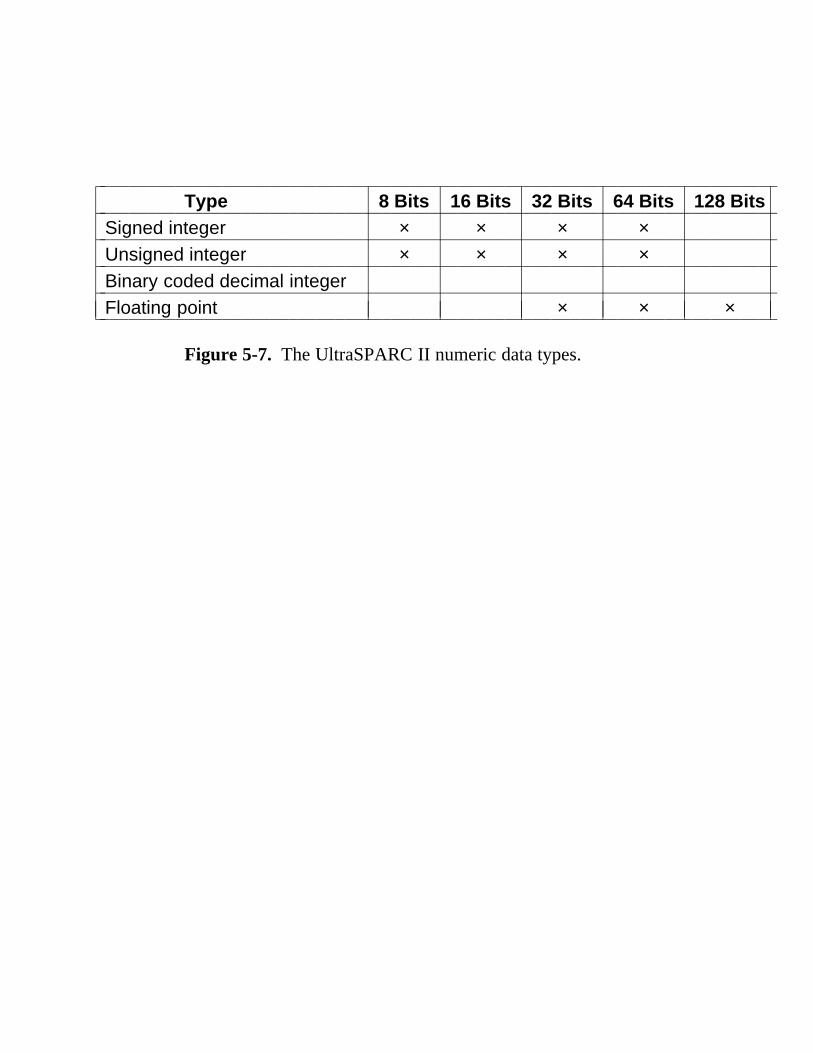
2222222222222222222222222222222222222222222222222222222222222222222222222Type 8 Bits 16 Bits 32 Bits 64 Bits 128 Bits2222222222222222222222222222222222222222222222222222222222222222222222222
Signed integer × × × ×2222222222222222222222222222222222222222222222222222222222222222222222222Unsigned integer × × × ×2222222222222222222222222222222222222222222222222222222222222222222222222Binary coded decimal integer2222222222222222222222222222222222222222222222222222222222222222222222222Floating point × × ×222222222222222222222222222222222222222222222222222222222222222222222222211111111
11111111
11111111
11111111
11111111
11111111
11111111
Figure 5-7. The UltraSPARC II numeric data types.

2222222222222222222222222222222222222222222222222222222222222222222222222Type 8 Bits 16 Bits 32 Bits 64 Bits 128 Bits2222222222222222222222222222222222222222222222222222222222222222222222222
Signed integer × × × ×2222222222222222222222222222222222222222222222222222222222222222222222222Unsigned integer2222222222222222222222222222222222222222222222222222222222222222222222222Binary coded decimal integer2222222222222222222222222222222222222222222222222222222222222222222222222Floating point × ×222222222222222222222222222222222222222222222222222222222222222222222222211111111
11111111
11111111
11111111
11111111
11111111
11111111
Figure 5-8. The JVM numeric data types.

OPCODE
(a) (b)
(c) (d)
OPCODE
OPCODE ADDR1 ADDR2 ADDR3OPCODE ADDRESS1 ADDRESS2
ADDRESS
Figure 5-9. Four common instruction formats: (a) Zero-address instruction. (b) One-address instruction (c) Two-address instruction. (d) Three-address instruction.

Instruction
Instruction
Instruction
Instruction
(a)
1 Word
Instruction
Instruction Instruction Instr. Instr.
Instruction
Instruction
Instruction
Instruction
Instruction
Instruction
(b)
1 Word
Instruction
Instruction
(c)
1 Word
Figure 5-10. Some possible relationships between instructionand word length.

15 13 11 9 7 5 3 114 12 10
Opcode
8 6 4 2
Address 1 Address 2 Address 3
Figure 5-11. An instruction with a 4-bit opcode and three 4-bitaddress fields.
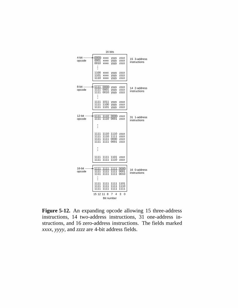
00004-bitopcode 15 3-address
instructions
xxxx
16 bits
Bit number
yyyy zzzz0001 xxxx yyyy zzzz0010 xxxx yyyy zzzz
1100 xxxx yyyy zzzz1101 xxxx yyyy zzzz1110 xxxx yyyy zzzz
11118-bitopcode 14 2-address
instructions
0000 yyyy zzzz1111 0001 yyyy zzzz1111 0010 yyyy zzzz
1111 1011 yyyy zzzz1111 1100 yyyy zzzz1111 1101 yyyy zzzz
1111 1110 1110 zzzz1111 1110 1111 zzzz1111 1111 0000 zzzz1111 1111 0001 zzzz
111112-bitopcode 31 1-address
instructions
1110 0000 zzzz1111 1110 0001 zzzz
1111 1111 1101 zzzz1111 1111 1110 zzzz
111116-bitopcode 16 0-address
instructions
1111 1111 00001111 1111 1111 00011111 1111 1111 0010
1111 1111 1111 11011111 1111 1111 11101111 1111 1111 1111
15 12 11 8 7 4 3 0
……
……
…
Figure 5-12. An expanding opcode allowing 15 three-addressinstructions, 14 two-address instructions, 31 one-address in-structions, and 16 zero-address instructions. The fields markedxxxx, yyyy, and zzzz are 4-bit address fields.

PREFIX
INSTRUCTION
Which operand is source?
Byte/word
SCALE INDEX BASE
MOD REC R/M
OPCODE MODE SIB DISPLACMENT IMMEDIATE
0 - 5
6 3321Bits Bits
332Bits
Bytes
1
1 - 2 0 - 1 0 - 1 0 - 4 0 - 4
Figure 5-13. The Pentium II instruction formats.

PC-RELATIVE DISPLACEMENT CALL4
302
PC-RELATIVE DISPLACEMENT BRANCH3
222
A
1
OP
3
COND
4
IMMEDIATE CONSTANT SETHI2
222
DEST
5
2 5 6 5 1 8 5
OP
3
Immediate1b DEST OPCODE SRC1 1 IMMEDIATE CONSTANT
3 Register1a DEST OPCODE SRC1 0 FP-OP SRC2Format
Figure 5-14. The original SPARC instruction formats.

CONSTINDEX
OPCODE VARIABLE LENGTH…9
OPCODE 32-BIT BRANCH OFFSET8
OPCODE INDEX CONST7
OPCODE INDEX 0#PARAMETERS6
OPCODE INDEX DIMENSIONS5
OPCODE4
OPCODE SHORT SHORT = index, constant or offset3
OPCODE BYTE BYTE = index, constant or type2
OPCODE1Format
Bits 8 8 8 88
Figure 5-15. The JVM instruction formats.
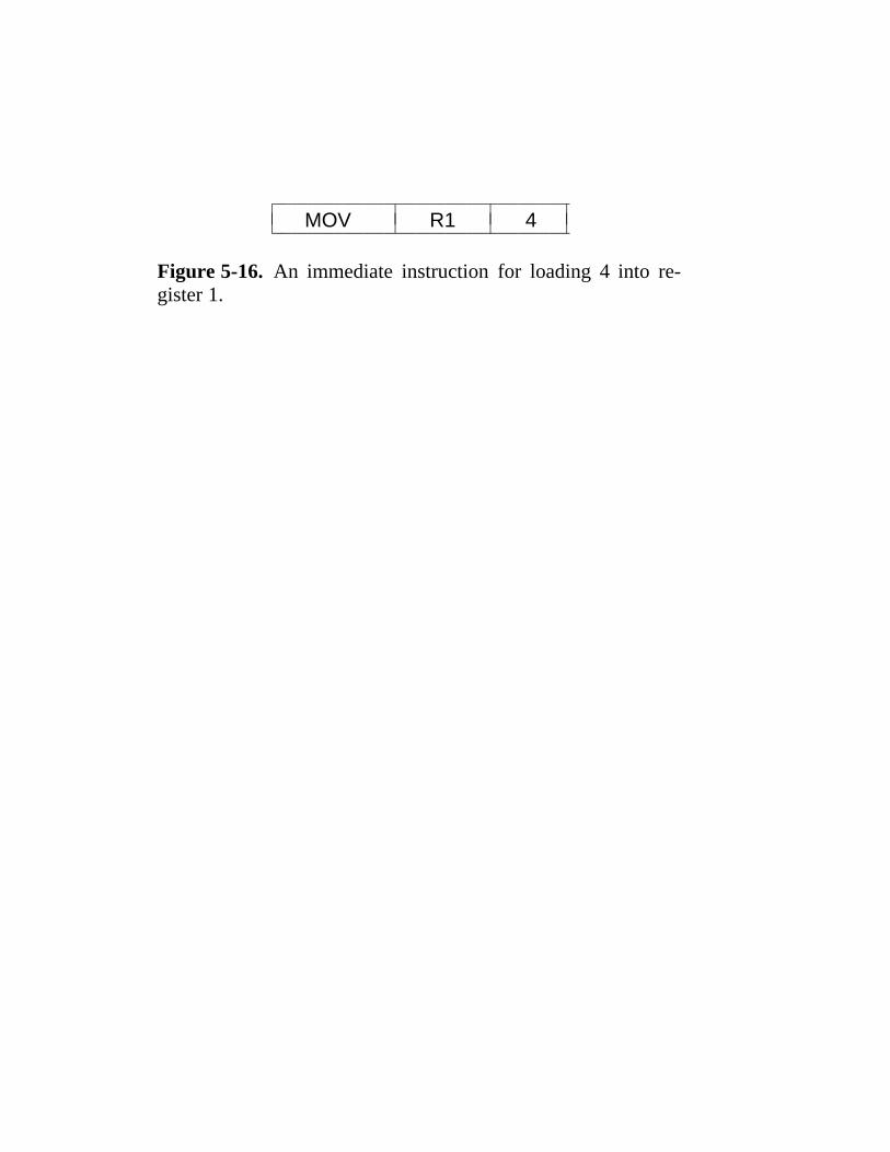
22222222222222222222222222222MOV R1 42222222222222222222222222222211 11 11 11
Figure 5-16. An immediate instruction for loading 4 into re-gister 1.
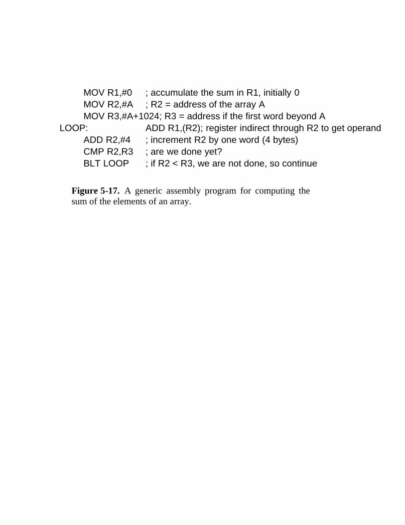
MOV R1,#0 ; accumulate the sum in R1, initially 0MOV R2,#A ; R2 = address of the array AMOV R3,#A+1024; R3 = address if the first word beyond A
LOOP: ADD R1,(R2); register indirect through R2 to get operandADD R2,#4 ; increment R2 by one word (4 bytes)CMP R2,R3 ; are we done yet?BLT LOOP ; if R2 < R3, we are not done, so continue
Figure 5-17. A generic assembly program for computing thesum of the elements of an array.

MOV R1,#0 ; accumulate the OR in R1, initially 0MOV R2,#0 ; R2 = index, i, of current product: A[i] AND B[i]MOV R3,#4096; R3 = first index value not to use
LOOP: MOV R4,A(R2); R4 = A[i]AND R4,B(R2) ; R4 = A[i] AND B[i]OR R1,R4 ; OR all the Boolean products into R1ADD R2,#4 ; i = i + 4 (step in units of 1 word = 4 bytes)CMP R2,R3 ; are we done yet?BLT LOOP ; if R2 < R3, we are not done, so continue
Figure 5-18. A generic assembly program for computing theOR of Ai AND Bi for two 1024-element arrays.

222222222222222222222222222222222222222222MOV R4 R2 12430022222222222222222222222222222222222222222211 11 11 11 11
Figure 5-19. A possible representation of MOV R4,A(R2).

⊥)C+B(xA
⊥
Switch
California
New York
Texas
Figure 5-20. Each railroad car represents one symbol in theformula to be converted from infix to reverse Polish notation.
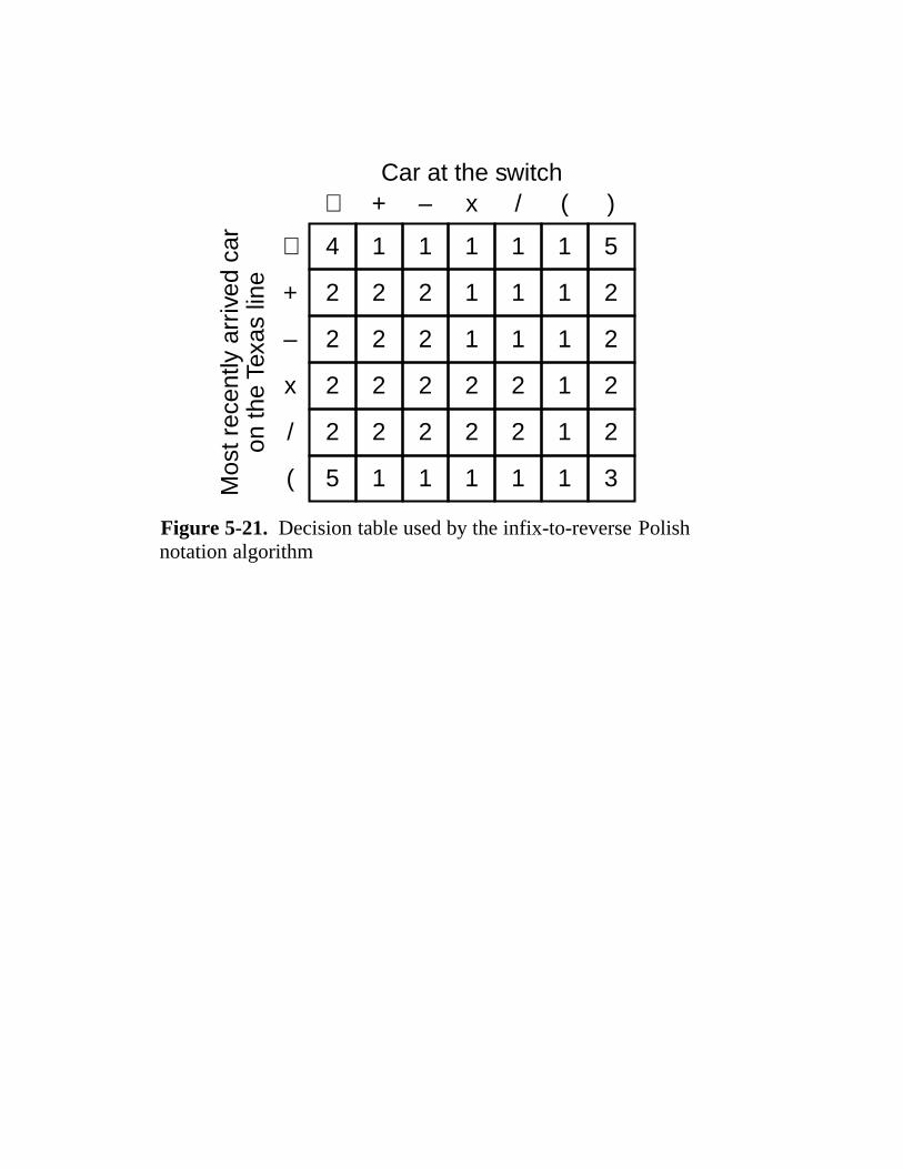
4 1 1 1 1 1 5
2 2 2 1 1 1 2
2 2 2 1 1 1 2
2 2 2 2 2 1 2
2 2 2 2 2 1 2
5
⊥
+
–
x
/
( 1 1 1 1 1 3
⊥ + – x / ( )Car at the switch
Mos
t rec
ently
arr
ived
car
on th
e Te
xas
line
Figure 5-21. Decision table used by the infix-to-reverse Polishnotation algorithm

22222222222222222222222222222222222222222222222222222222222222Infix Reverse Polish notation22222222222222222222222222222222222222222222222222222222222222
A + B × C A B C × +22222222222222222222222222222222222222222222222222222222222222A × B + C A B × C +22222222222222222222222222222222222222222222222222222222222222A × B + C × D A B × C D × +22222222222222222222222222222222222222222222222222222222222222(A + B) / (C − D) A B + C D − /22222222222222222222222222222222222222222222222222222222222222A × B / C A B × C /22222222222222222222222222222222222222222222222222222222222222((A + B) × C + D)/(E + F + G) A B + C × D + E F + G + /222222222222222222222222222222222222222222222222222222222222221
111111111
1111111111
1111111111
Figure 5-22. Some examples of infix expressions and their re-verse Polish notation equivalents.

2222222222222222222222222222222222222222222222222222222222222222Step Remaining string Instruction Stack2222222222222222222222222222222222222222222222222222222222222222
1 8 2 5 × + 1 3 2 × + 4 − / BIPUSH 8 822222222222222222222222222222222222222222222222222222222222222222 2 5 × + 1 3 2 × + 4 − / BIPUSH 2 8, 222222222222222222222222222222222222222222222222222222222222222223 5 × + 1 3 2 × + 4 − / BIPUSH 5 8, 2, 522222222222222222222222222222222222222222222222222222222222222224 × + 1 3 2 × + 4 − / IMUL 8, 1022222222222222222222222222222222222222222222222222222222222222225 + 1 3 2 × + 4 − / IADD 1822222222222222222222222222222222222222222222222222222222222222226 1 3 2 × + 4 − / BIPUSH 1 18, 122222222222222222222222222222222222222222222222222222222222222227 3 2 × + 4 − / BIPUSH 3 18, 1, 322222222222222222222222222222222222222222222222222222222222222228 2 × + 4 − / BIPUSH 2 18, 1, 3, 222222222222222222222222222222222222222222222222222222222222222229 × + 4 − / IMUL 18, 1, 62222222222222222222222222222222222222222222222222222222222222222
10 + 4 − / IADD 18, 7222222222222222222222222222222222222222222222222222222222222222211 4 − / BIPUSH 4 18, 7, 4222222222222222222222222222222222222222222222222222222222222222212 − / ISUB 18, 3222222222222222222222222222222222222222222222222222222222222222213 / IDIV 622222222222222222222222222222222222222222222222222222222222222221
1111111111111111111
11111111111111111111
11111111111111111111
11111111111111111111
11111111111111111111
Figure 5-23. Use of a stack to evaluate a reverse Polish notation formula.

OPCODE OFFSET3
OPCODE DEST SRC1 OFFSET2 1
OPCODE DEST SRC1 SRC21 0
8Bits 5 5 5 81
Figure 5-24. A simple design for the instruction formats of athree-address machine.

OPCODE MODE
8Bits 3
MODE
3
REG
5
OFFSET
4
REG
5
OFFSET
4
(Optional 32-bit direct address or offset)
(Optional 32-bit direct address or offset)
Figure 5-25. A simple design for the instruction formats of atwo-address machine.

222222222222222222222222222222222222222222222222222222222222222222222222MOD222222222222222222222222222222222222222222222222222222222222222222222222
R/M 00 01 10 11222222222222222222222222222222222222222222222222222222222222222222222222000 M[EAX] M[EAX + OFFSET8] M[EAX + OFFSET32] EAX or AL222222222222222222222222222222222222222222222222222222222222222222222222001 M[ECX] M[ECX + OFFSET8] M[ECX + OFFSET32] ECX or CL222222222222222222222222222222222222222222222222222222222222222222222222010 M[EDX] M[EDX + OFFSET8] M[EDX + OFFSET32] EDX or DL222222222222222222222222222222222222222222222222222222222222222222222222011 M[EBX] M[EBX + OFFSET8] M[EBX + OFFSET32] EBX or BL222222222222222222222222222222222222222222222222222222222222222222222222100 SIB SIB with OFFSET8 SIB with OFFSET32 ESP or AH222222222222222222222222222222222222222222222222222222222222222222222222101 Direct M[EBP + OFFSET8] M[EBP + OFFSET32] EBP or CH222222222222222222222222222222222222222222222222222222222222222222222222110 M[ESI] M[ESI + OFFSET8] M[ESI + OFFSET32] ESI or DH222222222222222222222222222222222222222222222222222222222222222222222222111 M[EDI] M[EDI + OFFSET8] M[EDI + OFFSET32] EDI or BH22222222222222222222222222222222222222222222222222222222222222222222222211
1111111111111
111111111111111
1111111111111
1111111111111
1111111111111
111111111111111
Figure 5-26. The Pentium II 32-bit addressing modes. M[x] isthe memory word at x.

Otherlocalvariables
Stackframe
a [0]
a [1]
a [2]
EBP + 8
EBP + 12
EBP + 16
SIB Mode refrencesM[4 * EAX + EBP + 8]
i in EAX
EBP
Figure 5-27. Access to a[i].

22222222222222222222222222222222222222222222222222222222222222222Addressing mode Pentium II UltraSPARC II JVM22222222222222222222222222222222222222222222222222222222222222222Immediate × × ×22222222222222222222222222222222222222222222222222222222222222222Direct ×22222222222222222222222222222222222222222222222222222222222222222Register × ×22222222222222222222222222222222222222222222222222222222222222222Register indirect ×22222222222222222222222222222222222222222222222222222222222222222Indexed × × ×22222222222222222222222222222222222222222222222222222222222222222Based-indexed ×22222222222222222222222222222222222222222222222222222222222222222Stack ×22222222222222222222222222222222222222222222222222222222222222222111111111111
111111111111
111111111111
111111111111
111111111111
Figure 5-28. A comparison of addressing modes.

i = 1; i = 1;L1: if (i > n) goto L2;
L1: first-statement; first-statement;. .. .. .last-statement; last-statementi = i + 1; i = i + 1;if (i < n) goto L1; goto L1;
L2:
(a) (b)
Figure 5-29. (a) Test-at-the-end loop. (b) Test-at-the-beginning loop.

Character available
Character received Character to display
Keyboard status
Interrupt enabled
Ready for next character
Display status
Interrupt enabled
Keyboard buffer Display buffer
Figure 5-30. Device registers for a simple terminal.
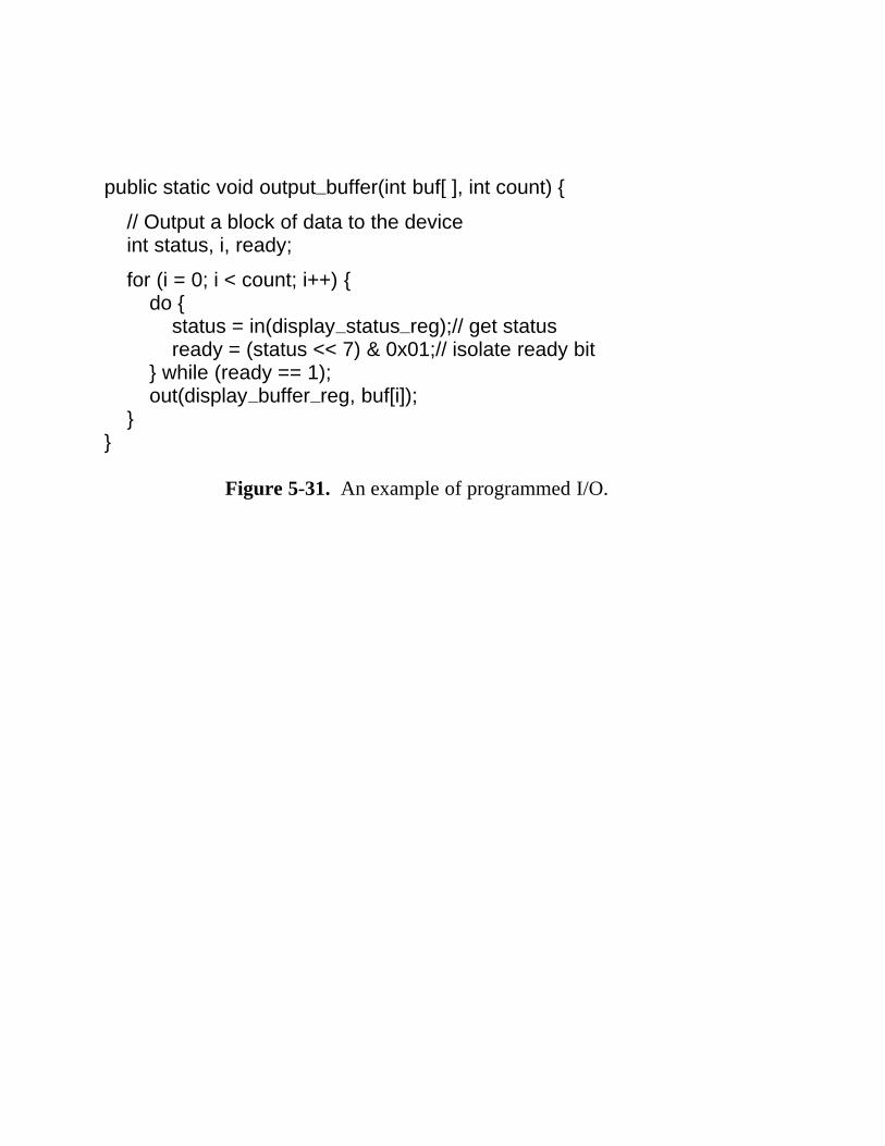
public static void output3buffer(int buf[ ], int count) {
// Output a block of data to the deviceint status, i, ready;
for (i = 0; i < count; i++) {do {
status = in(display3status3reg);// get statusready = (status << 7) & 0x01;// isolate ready bit
} while (ready == 1);out(display3buffer3reg, buf[i]);
}}
Figure 5-31. An example of programmed I/O.

Terminal
CPU DMA
Address
Count 1003241
Device Direction
Bus
Memory
100 RS232CController
……
Figure 5-32. A system with a DMA controller.
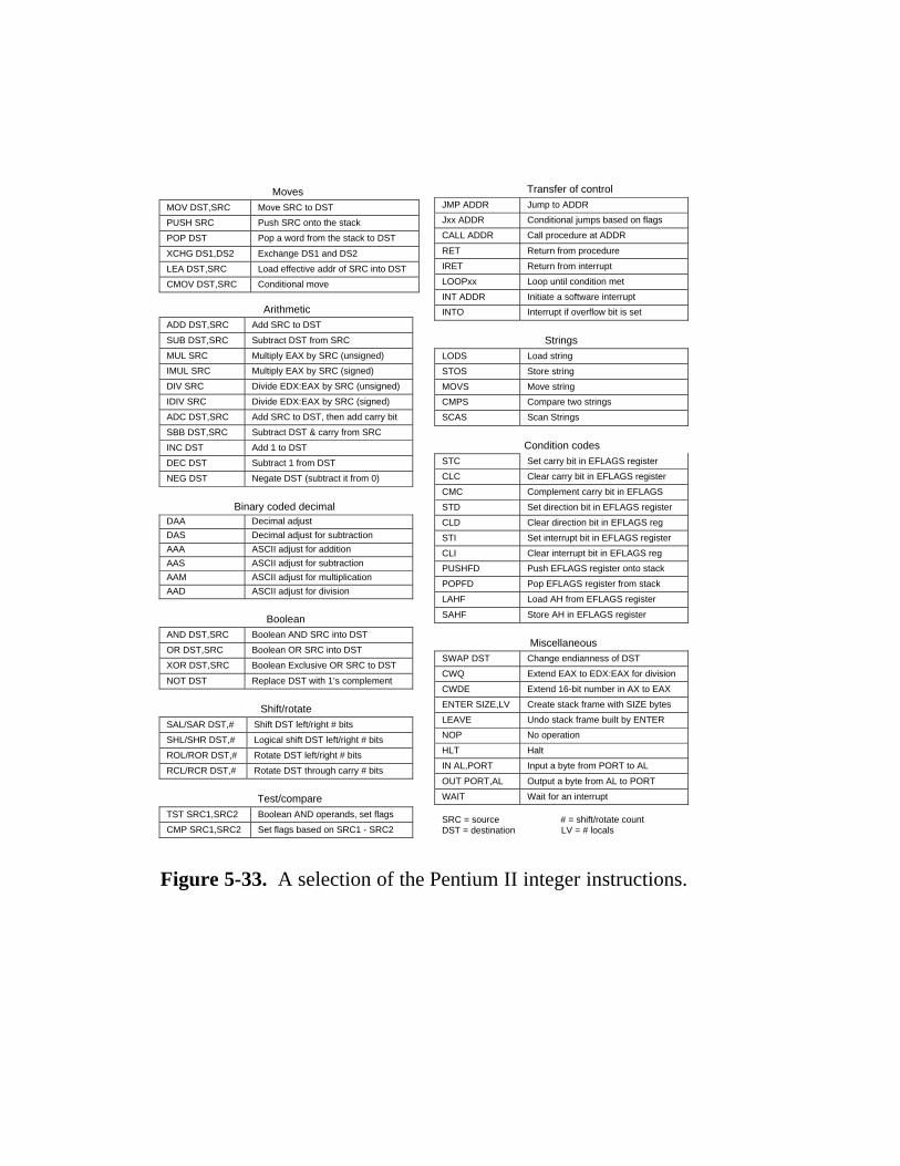
MovesMOV DST,SRC Move SRC to DST
PUSH SRC Push SRC onto the stack
POP DST Pop a word from the stack to DST
XCHG DS1,DS2 Exchange DS1 and DS2
LEA DST,SRC Load effective addr of SRC into DST
CMOV DST,SRC Conditional move
ArithmeticADD DST,SRC Add SRC to DST
SUB DST,SRC Subtract DST from SRC
MUL SRC Multiply EAX by SRC (unsigned)
IMUL SRC Multiply EAX by SRC (signed)
DIV SRC Divide EDX:EAX by SRC (unsigned)
IDIV SRC Divide EDX:EAX by SRC (signed)
ADC DST,SRC Add SRC to DST, then add carry bit
SBB DST,SRC Subtract DST & carry from SRC
INC DST Add 1 to DST
DEC DST Subtract 1 from DST
NEG DST Negate DST (subtract it from 0)
Binary coded decimalDAA Decimal adjust
DAS Decimal adjust for subtraction
AAA ASCII adjust for addition
AAS ASCII adjust for subtraction
AAM ASCII adjust for multiplication
AAD ASCII adjust for division
BooleanAND DST,SRC Boolean AND SRC into DST
OR DST,SRC Boolean OR SRC into DST
XOR DST,SRC Boolean Exclusive OR SRC to DST
NOT DST Replace DST with 1’s complement
Shift/rotateSAL/SAR DST,# Shift DST left/right # bits
SHL/SHR DST,# Logical shift DST left/right # bits
ROL/ROR DST,# Rotate DST left/right # bits
RCL/RCR DST,# Rotate DST through carry # bits
Test/compareTST SRC1,SRC2 Boolean AND operands, set flags
CMP SRC1,SRC2 Set flags based on SRC1 - SRC2
Transfer of controlJMP ADDR Jump to ADDR
Jxx ADDR Conditional jumps based on flags
CALL ADDR Call procedure at ADDR
RET Return from procedure
IRET Return from interrupt
LOOPxx Loop until condition met
INT ADDR Initiate a software interrupt
INTO Interrupt if overflow bit is set
StringsLODS Load string
STOS Store string
MOVS Move string
CMPS Compare two strings
SCAS Scan Strings
Condition codesSTC Set carry bit in EFLAGS register
CLC Clear carry bit in EFLAGS register
CMC Complement carry bit in EFLAGS
STD Set direction bit in EFLAGS register
CLD Clear direction bit in EFLAGS reg
STI Set interrupt bit in EFLAGS register
CLI Clear interrupt bit in EFLAGS reg
PUSHFD Push EFLAGS register onto stack
POPFD Pop EFLAGS register from stack
LAHF Load AH from EFLAGS register
SAHF Store AH in EFLAGS register
MiscellaneousSWAP DST Change endianness of DST
CWQ Extend EAX to EDX:EAX for division
CWDE Extend 16-bit number in AX to EAX
ENTER SIZE,LV Create stack frame with SIZE bytes
LEAVE Undo stack frame built by ENTER
NOP No operation
HLT Halt
IN AL,PORT Input a byte from PORT to AL
OUT PORT,AL Output a byte from AL to PORT
WAIT Wait for an interrupt
SRC = source # = shift/rotate countDST = destination LV = # locals
Figure 5-33. A selection of the Pentium II integer instructions.

LoadsLDSB ADDR,DST Load signed byte (8 bits)
LDUB ADDR,DST Load unsigned byte (8 bits)LDSH ADDR,DST Load signed halfword (16 bits)
LDUH ADDR,DST Load unsigned halfword (16)
LDSW ADDR,DST Load signed word (32 bits)
LDUW ADDR,DST Load unsigned word (32 bits)
LDX ADDR,DST Load extended (64-bits)
StoresSTB SRC,ADDR Store byte (8 bits)STH SRC,ADDR Store halfword (16 bits)
STW SRC,ADDR Store word (32 bits)
STX SRC,ADDR Store extended (64 btis)
ArithmeticADD R1,S2,DST Add
ADDCC “ Add and set icc
ADDC “ Add with carry
ADDCCC “ Add with carry and set icc
SUB R1,S2,DST Subtract
SUBCC “ Subtract and set icc
SUBC “ Subtract with carry
SUBCCC “ Subtract with carry and set icc
MULX R1,S2,DST Multiply
SDIVX R1,S2,DST Signed divideUDIVX R1,S2,DST Unsigned divide
TADCC R1,S2,DST Tagged add
Shifts/rotatesSLL R1,S2,DST Shift left logical (64 bits)
SLLX R1,S2,DST Shift left logical extended (64)
SRL R1,S2,DST Shift right logical (32 bits)
SRLX R1,S2,DST Shift right logical extended (64)
SRA R1,S2,DST Shift right arithmetic (32 bits)
SRAX R1,S2,DST Shift right arithmetic ext. (64)
BooleanAND R1,S2,DST Boolean AND
ANDCC “ Boolean AND and set iccANDN “ Boolean NAND
ANDNCC “ Boolean NAND and set icc
OR R1,S2,DST Boolean OR
ORCC “ Boolean OR and set icc
ORN “ Boolean NOR
ORNCC “ Boolean NOR and set iccXOR R1,S2,DST Boolean XOR
XORCC “ Boolean XOR and set icc
XNOR “ Boolean EXCLUSIVE NOR
XNORCC “ Boolean EXCL. NOR and set icc
Transfer of controlBPcc ADDR Branch with prediction
BPr SRC,ADDR Branch on registerCALL ADDR Call procedure
RETURN ADDR Return from procedure
JMPL ADDR,DST Jump and Link
SAVE R1,S2,DST Advance register windows
RESTORE “ Restore register windows
Tcc CC,TRAP# Trap on conditionPREFETCH FCN Prefetch data from memory
LDSTUB ADDR,R Atomic load/store
MEMBAR MASK Memory barrier
MiscellaneousSETHI CON,DST Set bits 10 to 31
MOVcc CC,S2,DST Move on condition
MOVr R1,S2,DST Move on register
NOP No operationPOPC S1,DST Population count
RDCCR V,DST Read condition code register
WRCCR R1,S2,V Write condition code register
RDPC V,DST Read program counter
SRC = source registerDST = destination registerR1 = source registerS2 = source: register or immediateADDR = memory address
TRAP# = trap numberFCN = function codeMASK = operation typeCON = constantV = register designator
CC = condition code setR =destination register
cc = conditionr = LZ,LEZ,Z,NZ,GZ,GEZ
Figure 5-34. The primary UltraSPARC II integer instructions.

22222222222222222222222222222222222222222222222222222222222222222222222Instruction How to do it22222222222222222222222222222222222222222222222222222222222222222222222
MOV SRC,DST OR SRC with G0 and store the result DST22222222222222222222222222222222222222222222222222222222222222222222222CMP SRC1,SRC2 SUBCC SRC2 from SRC1 and store the result in G022222222222222222222222222222222222222222222222222222222222222222222222TST SRC ORCC SRC1 with G0 and store the result in G022222222222222222222222222222222222222222222222222222222222222222222222NOT DST XNOR DST with G022222222222222222222222222222222222222222222222222222222222222222222222NEG DST SUB DST from G0 and store in DST22222222222222222222222222222222222222222222222222222222222222222222222INC DST ADD 1 to DST (immediate operand)22222222222222222222222222222222222222222222222222222222222222222222222DEC DST SUB 1 from DST (immediate operand)22222222222222222222222222222222222222222222222222222222222222222222222CLR DST OR G0 with G0 and store in DST22222222222222222222222222222222222222222222222222222222222222222222222NOP SETHI G0 to 022222222222222222222222222222222222222222222222222222222222222222222222RET JMPL %I7+8,%G0222222222222222222222222222222222222222222222222222222222222222222222221111111111111111
1111111111111111
1111111111111111
Figure 5-35. Some simulated UltraSPARC II instructions.
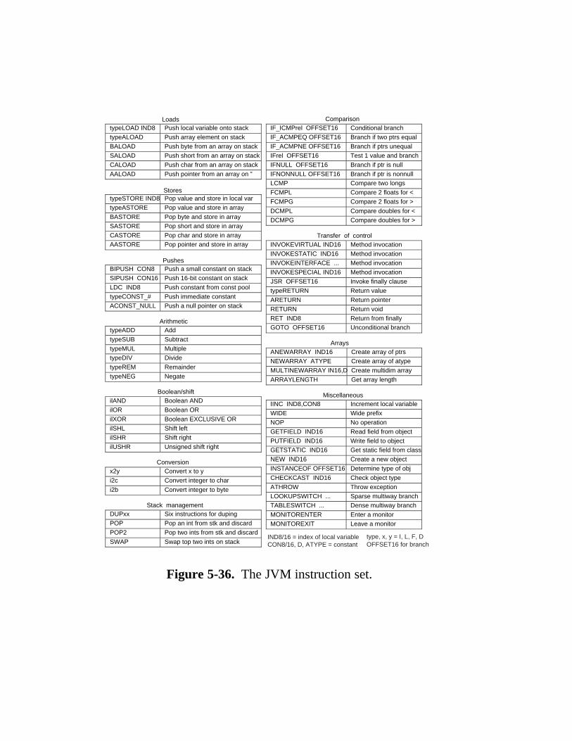
LoadstypeLOAD IND8 Push local variable onto stack
typeALOAD Push array element on stack
BALOAD Push byte from an array on stack
SALOAD Push short from an array on stack
CALOAD Push char from an array on stack
AALOAD Push pointer from an array on ”
StorestypeSTORE IND8 Pop value and store in local var
typeASTORE Pop value and store in array
BASTORE Pop byte and store in array
SASTORE Pop short and store in array
CASTORE Pop char and store in arrayAASTORE Pop pointer and store in array
PushesBIPUSH CON8 Push a small constant on stack
SIPUSH CON16 Push 16-bit constant on stack
LDC IND8 Push constant from const pool
typeCONST_# Push immediate constant
ACONST_NULL Push a null pointer on stack
ArithmetictypeADD Add
typeSUB Subtract
typeMUL Multiple
typeDIV Divide
typeREM Remainder
typeNEG Negate
Boolean/shiftilAND Boolean AND
ilOR Boolean OR
ilXOR Boolean EXCLUSIVE OR
ilSHL Shift left
ilSHR Shift right
ilUSHR Unsigned shift right
Conversionx2y Convert x to y
i2c Convert integer to char
i2b Convert integer to byte
Stack managementDUPxx Six instructions for duping
POP Pop an int from stk and discard
POP2 Pop two ints from stk and discard
SWAP Swap top two ints on stack
ComparisonIF_ICMPrel OFFSET16 Conditional branch
IF_ACMPEQ OFFSET16 Branch if two ptrs equal
IF_ACMPNE OFFSET16 Branch if ptrs unequal
IFrel OFFSET16 Test 1 value and branch
IFNULL OFFSET16 Branch if ptr is null
IFNONNULL OFFSET16 Branch if ptr is nonnullLCMP Compare two longs
FCMPL Compare 2 floats for <
FCMPG Compare 2 floats for >
DCMPL Compare doubles for <
DCMPG Compare doubles for >
Transfer of controlINVOKEVIRTUAL IND16 Method invocation
INVOKESTATIC IND16 Method invocation
INVOKEINTERFACE ... Method invocation
INVOKESPECIAL IND16 Method invocation
JSR OFFSET16 Invoke finally clause
typeRETURN Return value
ARETURN Return pointer
RETURN Return void
RET IND8 Return from finallyGOTO OFFSET16 Unconditional branch
ArraysANEWARRAY IND16 Create array of ptrs
NEWARRAY ATYPE Create array of atype
MULTINEWARRAY IN16,D Create multidim array
ARRAYLENGTH Get array length
MiscellaneousIINC IND8,CON8 Increment local variable
WIDE Wide prefix
NOP No operation
GETFIELD IND16 Read field from object
PUTFIELD IND16 Write field to objectGETSTATIC IND16 Get static field from class
NEW IND16 Create a new object
INSTANCEOF OFFSET16 Determine type of obj
CHECKCAST IND16 Check object type
ATHROW Throw exception
LOOKUPSWITCH ... Sparse multiway branchTABLESWITCH ... Dense multiway branch
MONITORENTER Enter a monitor
MONITOREXIT Leave a monitor
IND8/16 = index of local variableCON8/16, D, ATYPE = constant
type, x, y = I, L, F, D OFFSET16 for branch
Figure 5-36. The JVM instruction set.

Pro
gram
cou
nter
Time
(a)
Time
(b)
Pro
gram
cou
nter
Jumps
Figure 5-37. Program counter as a function of time(smoothed). (a) Without branches. (b) With branches.

Peg 2Peg 1 Peg 3
Figure 5-38. Initial configuration for the Towers of Hanoiproblem for five disks.
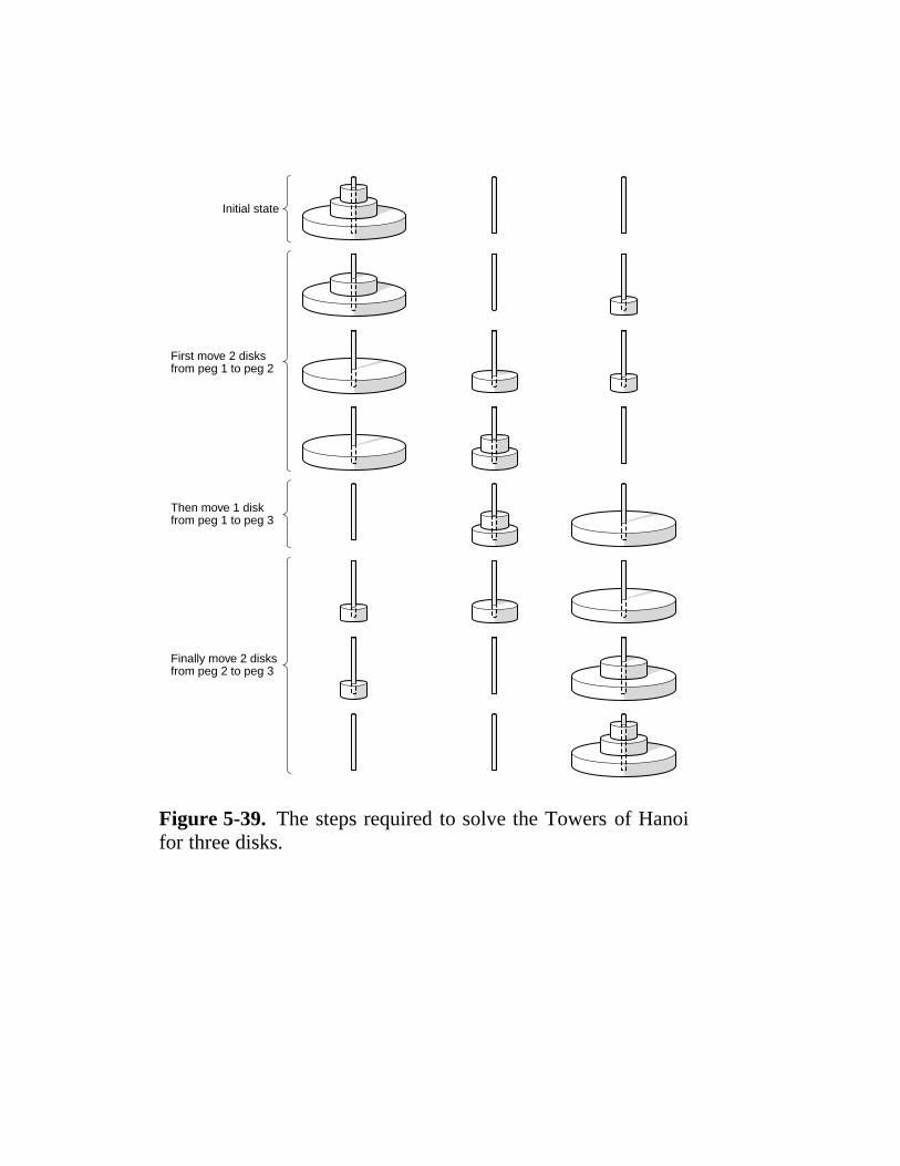
Initial state
First move 2 disksfrom peg 1 to peg 2
Then move 1 diskfrom peg 1 to peg 3
Finally move 2 disksfrom peg 2 to peg 3
Figure 5-39. The steps required to solve the Towers of Hanoifor three disks.

public void towers(int n, int i, int j) {int k;
if (n == 1)System.out.println("Move a disk from " + i + " to " + j);
else {k = 6 − i − j;towers(n − 1, i, k);towers(1, i, j);towers(n − 1, k, j);
}}
Figure 5-40. A procedure for solving the Towers of Hanoi.
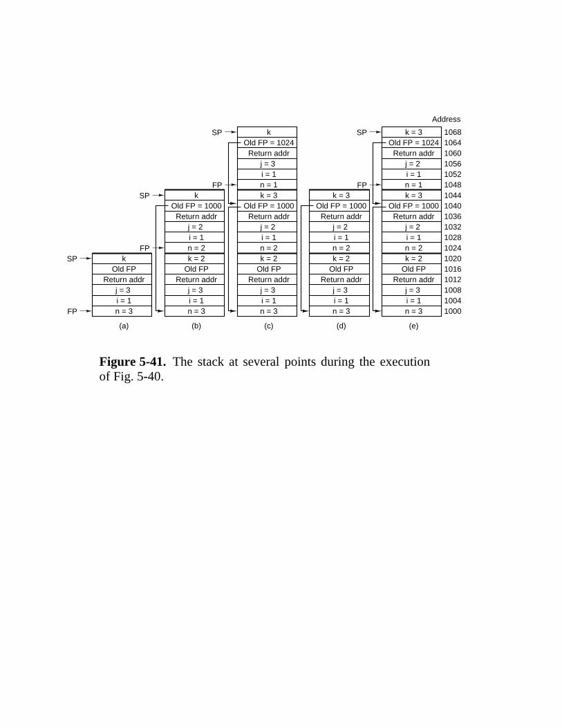
n = 3i = 1j = 3
Return addrOld FP
k
n = 3i = 1j = 3
Return addrOld FPk = 2
n = 3i = 1j = 3
Return addrOld FPk = 2
n = 3i = 1j = 3
Return addrOld FPk = 2
n = 3
(a) (b) (c) (d) (e)
i = 1j = 3
Return addrOld FPk = 2
n = 2i = 1j = 2
Return addrOld FP = 1000
k
n = 2i = 1j = 2
Return addrOld FP = 1000
k = 3
n = 2i = 1j = 2
Return addrOld FP = 1000
k = 3
n = 2i = 1j = 2
Return addrOld FP = 1000
k = 3n = 1i = 1j = 3
Return addrOld FP = 1024
k
n = 1i = 1j = 2
Return addrOld FP = 1024
k = 3
100010041008101210161020102410281032103610401044104810521056106010641068
Address
FP
SP
SP
FP
FP
SP
FP
SP
Figure 5-41. The stack at several points during the executionof Fig. 5-40.

(a)
Callingprocedure
(b)
Calledprocedure
A calledfrom mainprogram
A returnsto mainprogram
CALL
CALL
CALL
RETURN
RETURN
RETURN
Figure 5-42. When a procedure is called, execution of the pro-cedure always begins at the first statement of the procedure.

(a)
A calledfrom mainprogram
A returnsto mainprogram
(b)
RESUME B
RESUME A
RESUME B
RESUME B
RESUME A
RESUME A
Figure 5-43. When a coroutine is resumed, execution begins atthe statement where it left off the previous time, not at the be-ginning.

0 10 15 20 25 35 40
Disk interruptpriority 4 held pending
RS232 ISR finishesdisk interrupt occurs
Disk ISR finishes
Printer ISR finishes
RS232 interruptpriority 5
Printer interruptpriority 2
Userprogram
PrinterISR
RS232ISR
DiskISR
PrinterISR
Userprogram
Time
StackUserPrinter
User UserPrinter
User
Figure 5-44. Time sequence of multiple interrupt example.

.586 ; compile for Pentium (as opposed to 8088 etc.).MODEL FLATPUBLIC 3towers ; export ’towers’EXTERN 3printf:NEAR ; import printf.CODE3towers: PUSH EBP; save EBP (frame pointer)
MOV EBP, ESP ; set new frame pointer above ESPCMP [EBP+8], 1 ; if (n == 1)JNE L1 ; branch if n is not 1MOV EAX, [EBP+16] ; printf(" ...", i, j);PUSH EAX ; note that parameters i, j and the formatMOV EAX, [EBP+12] ; string are pushed onto the stackPUSH EAX ; in reverse order. This is the C calling conventionPUSH OFFSET FLAT:format; offset flat means the address of formatCALL 3printf ; call printfADD ESP, 12 ; remove params from the stackJMP Done ; we are finished
L1: MOV EAX, 6 ; start k = 6 − i − jSUB EAX, [EBP+12] ; EAX = 6 − iSUB EAX, [EBP+16] ; EAX = 6 − i − jMOV [EBP+20], EAX ; k = EAXPUSH EAX ; start towers(n − 1, i, k)MOV EAX, [EBP+12] ; EAX = iPUSH EAX ; push iMOV EAX, [EBP+8] ; EAX = nDEC EAX ; EAX = n − 1PUSH EAX ; push n − 1CALL 3towers ; call towers(n − 1, i, 6 − i − j)ADD ESP, 12 ; remove params from the stackMOV EAX, [EBP+16] ; start towers(1, i, j)PUSH EAX ; push jMOV EAX, [EBP+12] ; EAX = iPUSH EAX ; push iPUSH 1 ; push 1CALL 3towers ; call towers(1, i, j)ADD ESP, 12 ; remove params from the stackMOV EAX, [EBP+12] ; start towers(n − 1, 6 − i − j, i)PUSH EAX ; push iMOV EAX, [EBP+20] ; push 20PUSH EAX ; push kMOV EAX, [EBP+8] ; EAX = nDEC EAX ; EAX = n−1PUSH EAX ; push n − 1CALL 3towers ; call towers(n − 1, 6 − i − j, i)ADD ESP, 12 ; adjust stack pointer
Done: LEAVE ; prepare to exitRET 0 ; return to the caller
.DATAformat DB "Move disk from %d to %d\n"; format stringEND Figure 5-45. The Towers of Hanoi for the Pentium II.
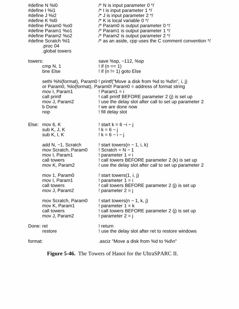
#define N %i0 /* N is input parameter 0 */#define I %i1 /* I is input parameter 1 */#define J %i2 /* J is input parameter 2 */#define K %l0 /* K is local variable 0 */#define Param0 %o0 /* Param0 is output parameter 0 */#define Param1 %o1 /* Param1 is output parameter 1 */#define Param2 %o2 /* Param2 is output parameter 2 */#define Scratch %l1 /* as an aside, cpp uses the C comment convention */
.proc 04
.global towers
towers: save %sp, −112, %spcmp N, 1 ! if (n == 1)bne Else ! if (n != 1) goto Else
sethi %hi(format), Param0 ! printf("Move a disk from %d to %d\n", i, j)or Param0, %lo(format), Param0! Param0 = address of format stringmov I, Param1 ! Param1 = icall printf ! call printf BEFORE parameter 2 (j) is set upmov J, Param2 ! use the delay slot after call to set up parameter 2b Done ! we are done nownop ! fill delay slot
Else: mov 6, K ! start k = 6 −i − jsub K, J, K ! k = 6 − jsub K, I, K ! k = 6 − i − j
add N, −1, Scratch ! start towers(n − 1, i, k)mov Scratch, Param0 ! Scratch = N − 1mov I, Param1 ! parameter 1 = icall towers ! call towers BEFORE parameter 2 (k) is set upmov K, Param2 ! use the delay slot after call to set up parameter 2
mov 1, Param0 ! start towers(1, i, j)mov I, Param1 ! parameter 1 = icall towers ! call towers BEFORE parameter 2 (j) is set upmov J, Param2 ! parameter 2 = j
mov Scratch, Param0 ! start towers(n − 1, k, j)mov K, Param1 ! parameter 1 = kcall towers ! call towers BEFORE parameter 2 (j) is set upmov J, Param2 ! parameter 2 = j
Done: ret ! returnrestore ! use the delay slot after ret to restore windows
format: .asciz "Move a disk from %d to %d\n"
Figure 5-46. The Towers of Hanoi for the UltraSPARC II.

ILOAD30 // local 0 = n; push nICONST31 // push 1IF3ICMPNE L1 // if (n != 1) goto L1
GETSTATIC #13 // n == 1; this code handles the println statementNEW #7 // allocate buffer for the string to be builtDUP // duplicate the pointer to the bufferLDC #2 // push pointer to string "move a disk from "INVOKESPECIAL #10 // copy the string to the bufferILOAD31 // push iINVOKEVIRTUAL #11 // convert i to string and append to the new bufferLDC #1 // push pointer to string " to "INVOKEVIRTUAL #12 // append this string to the bufferILOAD32 // push jINVOKEVIRTUAL #11 // convert j to string and append to bufferINVOKEVIRTUAL #15 // string conversionINVOKEVIRTUAL #14 // call printlnRETURN // return from towers
L1: BIPUSH 6 // Else part: compute k = 6 − i − jILOAD31 // local 1 = i; push iISUB // top-of-stack = 6 − iILOAD32 // local 2 = j; push jISUB // top-of-stack = 6 − i − jISTORE33 // local 3 = k = 6 − i − j; stack is now empty
ILOAD30 // start working on towers(n − 1, i, k); push nICONST31 // push 1ISUB // top-of-stack = n − 1ILOAD31 // push iILOAD33 // push kINVOKESTATIC #16 // call towers(n − 1, 1, k)
ICONST31 // start working on towers(1, i, j); push 1ILOAD31 // push iILOAD32 // push jINVOKESTATIC #16 // call towers(1, i, j)
ILOAD30 // start working on towers(n − 1, k, j); push nICONST31 // push 1ISUB // top-of-stack = n − 1ILOAD33 // push kILOAD32 // push jINVOKESTATIC #16 // call towers(n − 1, k, j)RETURN // return from towers
Figure 5-47. The Towers of Hanoi for JVM.

Instructionscan bechainedtogether
INSTRUCTION 1 INSTRUCTION 2 INSTRUCTION 3 TEMPLATE
INSTRUCTION 1 INSTRUCTION 2 INSTRUCTION 3 TEMPLATE
INSTRUCTION 1 INSTRUCTION 2 INSTRUCTION 3 TEMPLATE
R2R1
PREDICATEREGISTER
R3
Figure 5-48. IA-64 is based on bundles of three instructions.

if (R1 == 0) CMP R1,0 CMOVZ R2,R3,R1R2 = R3; BNE L1
MOV R2,R3L1:
(a) (b) (c)
Figure 5-49. (a) An if statement. (b) Generic assembly codefor (a). (c) A conditional instruction.

if (R1 == 0) { CMP R1,0 CMOVZ R2,R3,R1R2 = R3; BNE L1 CMOVZ R4,R5,R1R4 = R5; MOV R2,R3 CMOVN R6,R7,R1
} else { MOV R4.R5 CMOVN R8,R9,R1R6 = R7; BR L2R8 = R9; L1: MOV R6,R7
} MOV R8,R9L2:
(a) (b) (c)
Figure 5-50. (a) An if statement. (b) Generic assembly codefor (a). (c) Conditional execution.

if (R1 == R2) CMP R1,R2 CMPEQ R1,R2,P4R3 = R4 + R5; BNE L1 <P4> ADD R3,R4,R5
else MOV R3,R4 <P5> SUB R6,R4,R5R6 = R4 − R5 ADD R3,R5
BR L2L1: MOV R6,R4
SUB R6,R5L2:
(a) (b) (c)
Figure 5-51. (a) An if statement. (b) Generic assembly codefor (a). (c) Predicated execution.

388 THE INSTRUCTION SET ARCHITECTURE LEVEL CHAP. 5
5.8 THE INTEL IA-64
Intel is rapidly getting to the point where it has just about squeezed every lastdrop of juice out of the IA-32 ISA and the Pentium II line of processors. Newmodels can still benefit from advances in manufacturing technology, which meanssmaller transistors (hence faster clock speeds). However, finding new tricks tospeed up the implementation even more is getting harder and harder as the con-straints imposed by the IA-32 ISA are looming larger all the time.
The only real solution is to abandon the IA-32 as the main line of develop-ment and go to a completely new ISA. This is, in fact, what Intel intends to do.The new architecture, developed jointly by Intel and Hewlett Packard, is calledthe IA-64. It is a full 64-bit machine from beginning to end. A whole series ofCPUs implementing this architecture is expected in the coming years. The firstimplementation, code named the Merced (after somebody’s favorite Californiariver), is a high-end CPU, but eventually there will be a whole spectrum of CPUs,from high-end servers to entry-level desktop models.
Given the importance to the computer industry of anything Intel does, it isworth taking a look at the IA-64 architecture (and by implication, the Merced).However, that aside, the key ideas beyond the IA-64 are already well knownamong researchers in the field and may well surface in other designs as well. Infact, some of them are already present in various forms in (experimental) systems.In the following sections we will look at the nature of the problem Intel is facing,the model that IA-64 adopts to deal with it, how some of the key ideas work, andwhat might happen.
5.8.1 The Problem with the Pentium II
The main fact of life that causes all the trouble is that IA-32 is an ancient ISAwith all the wrong properties for current technology. It is a CISC ISA withvariable-length instructions and a myriad of different formats that are hard todecode quickly on the fly. Current technology works best with RISC ISAs thathave one instruction length and a fixed length opcode that is easy to decode. TheIA-32 instructions can be broken up into RISC-like micro-operations at executiontime, but doing so requires hardware (chip area), takes time, and adds complexityto the design. That is strike one.
The IA-32 is also a two-address memory-oriented ISA. Most instructions ref-erence memory, and most programmers and compilers think nothing of referenc-ing memory all the time. Current technology favors load/store ISAs that onlyreference memory to get the operands into registers but otherwise perform alltheir calculations using three-address memory register instructions. And withCPU clock speeds going up much faster than memory speeds, the problem will getworse with time. That is strike two.

SEC. 5.8 THE INTEL IA-64 389
The IA-32 also has a small and irregular register set. Not only does this tiecompilers in knots, but the small number of general-purpose registers (four or six,depending on how you count ESI and EDI) requires intermediate results to bespilled into memory all the time, generating extra memory references even whenthey are not logically needed. That is strike three. The IA-32 is out.
Now let us start the second inning. The small number of registers causesmany dependences, especially unnecessary WAR dependences, because resultshave to go somewhere and there are no extra registers available. Getting aroundthe lack of registers requires the implementation to do renaming internally—a ter-rible hack if ever there was one—to secret registers inside the reorder buffer. Toavoid blocking on cache misses too often, instructions have to be executed out oforder. However, the IA-32’s semantics specify precise interrupts, so the out-of-order instructions have to be retired in order. All of these things require a lot ofvery complex hardware. Strike four.
Doing all this work quickly requires a very deep (12-stage) pipeline. In turn,the deep pipeline means that instructions are entered into it 11 cycles before theywill be finished. Consequently, very accurate branch prediction is essential tomake sure the right instructions are being entered into the pipeline. Because amisprediction requires the pipeline to be flushed, at great cost, even a fairly lowmisprediction rate can cause a substantial performance degradation. Strike five.
To alleviate the problems with mispredictions, the processor has to do specu-lative execution, with all the problems that entails, especially when memory refer-ences on the wrong path cause an exception. Strike six.
We are not going to play the whole baseball game here, but it should be clearby now that there is a real problem. And we have not even mentioned the factthat IA-32’s 32-bit addresses limit individual programs to 4 GB of memory, whichis a growing problem on high-end servers.
All in all, the situation with IA-32 can be favorably compared to the state ofcelestial mechanics just prior to Copernicus. The then-current theory dominatingastronomy was that the earth was fixed and motionless in space and that theplanets moved in circles with epicycles around it. However, as observations gotbetter and more deviations from this model could be clearly observed, epicycleswere added to the epicycles until the whole model just collapsed from its internalcomplexity
Intel is in the same pickle now. A huge fraction of all the transistors on thePentium II are devoted to decomposing CISC instructions, figuring out what canbe done in parallel, resolving conflicts, making predictions, repairing the conse-quences of incorrect predictions and other bookkeeping, leaving surprisingly fewover for doing the real work the user asked for. The conclusion that Intel is beinginexorably driven to is the only sane conclusion: junk the whole thing (IA-32) andstart all over with a clean slate (IA-64).

390 THE INSTRUCTION SET ARCHITECTURE LEVEL CHAP. 5
5.8.2 The IA-64 Model: Explicitly Parallel Instruction Computing
The starting point for IA-64 was a high-end 64-bit RISC processor (of whichthe UltraSPARC II is one of many current examples). Since the IA-64 wasdesigned jointly with Hewlett Packard, no doubt HP’s PA-RISC architecture wasthe real basis, but all state-of-the-art RISC machines are similar enough that ourdiscussion of the UltraSPARC II is still highly germane. The Merced is a dual-mode processor, with the capability of running both IA-32 and IA-64 programs,but we will focus only on the IA-64 part in the discussion below.
The IA-64 architecture is a load/store architecture with 64-bit addresses and64-bit wide registers. There are 64 general registers available to IA-64 programs(and additional registers available to IA-32 programs). All instructions have thesame fixed format: an opcode, two 6-bit source register fields, a 6-bit destinationregister field, and another 6-bit field to be discussed later on. Most instructionstake two register operands, perform some computation on them, and put the resultback in the destination register. Many functional units are available for doing dif-ferent operations in parallel. So far, nothing unusual. Most RISC machines havean architecture pretty much like this.
What is unusual is the idea of a bundle of related instructions. Instructionscome in groups of three, called a bundle, as shown in Fig. 5-1. Each 128-bit bitbundle contains three 40-bit fixed-format instructions and an 8-bit template. Bun-dles can be chained together using an end-of-bundle bit, so more than threeinstructions can be present in one bundle. The template contains informationabout which instructions can be executed in parallel. This scheme, plus theexistence of so many registers, allows the compiler to isolate blocks of instruc-tions and tell the CPU that they can be executed in parallel. Thus the compilermust reorder instructions, check for dependences, make sure there are functionalunits available, etc., instead of the hardware. The idea is that by exposing theinternal workings of the machine and telling compiler writers to make sure thateach bundle consists of compatible instructions, the job of scheduling the RISCinstructions is moved from the hardware (at run time) to the compiler (at compiletime). For this reason, the model is called EPIC (Explicitly Parallel InstructionComputing).
There are several advantages to doing instruction scheduling at compile time.First, since the compiler is now doing all the work, the hardware can be muchsimpler, saving millions of transistors for other useful functions, such as largerlevel 1 caches. Second, for any given program, the scheduling has to be doneonly once, at compile time. Third, since the compiler is now doing all the work, itwill be possible for a software vendor to use a compiler that spends hours optimiz-ing its program and have all the users have the benefit every time the program isrun.
The idea of bundles of instructions can be used to create a whole family ofprocessors. On the low-end CPUs, one bundle may be issued per clock cycle.

SEC. 5.8 THE INTEL IA-64 391
Instructionscan bechainedtogether
INSTRUCTION 1 INSTRUCTION 2 INSTRUCTION 3 TEMPLATE
INSTRUCTION 1 INSTRUCTION 2 INSTRUCTION 3 TEMPLATE
INSTRUCTION 1 INSTRUCTION 2 INSTRUCTION 3 TEMPLATE
R2R1
PREDICATEREGISTER
R3
Figure 5-1. IA-64 is based on bundles of three instructions.
The CPU may wait until all the instructions have completed before issuing thenext bundle. On high-end CPUs, it may be possible to issue multiple bundles dur-ing the same clock cycle, analogous to current superscalar designs. Also, onhigh-end CPUs, the processor may begin issuing instructions from a new bundlebefore all instructions from the previous bundle have completed. Of course, itneeds to check to see if the registers and functional unit needed are available, butit does not have to check to see if other instructions from its own bundle are inconflict with it as the compiler has guaranteed that this is not the case.
5.8.3 Predication
Another important feature of IA-64 is the new way it deals with conditionalbranches. If there were a way to get rid of most of them, CPUs could be mademuch simpler and faster. At first thought it might seem that getting rid of condi-tional branches would be impossible because programs are full of if statements.However, IA-64 uses a technique called predication that can greatly reduce theirnumber (August et al., 1998; and Hwu, 1998). We will now briefly describe it.
In current machines, all instructions are unconditional in the sense that whenthe CPU hits an instruction, it just carries the instruction out. There is no internaldebate of the form: ‘‘To do or not to do, that is the question?’’ In contrast, in apredicated architecture, instructions contain conditions (predicates) telling whenthey should be executed and when not. This paradigm shift from unconditionalinstructions to predicated instructions is what makes it possible to get rid of(many) conditional branches. Instead of having to make a choice between onesequence of unconditional instructions or another sequence of unconditionalinstructions, all the instructions are merged into a single sequence of predicated

392 THE INSTRUCTION SET ARCHITECTURE LEVEL CHAP. 5
instructions, using different predicates for different instructions.To see how predication works, let us start with the simple example of Fig. 5-
2, which shows conditional execution, a precursor to predication. In Fig. 5-2(a)we see an if statement. In Fig. 5-2(b) we see its translation into three instructions:a comparison, a conditional branch, and a move instruction.
if (R1 == 0) CMP R1,0 CMOVZ R2,R3,R1R2 = R3; BNE L1
MOV R2,R3L1:
(a) (b) (c)
Figure 5-2. (a) An if statement. (b) Generic assembly code for (a). (c) A con-ditional instruction.
In Fig. 5-2(c) we get rid of the conditional branch by using a new instruction,CMOVZ, which is a conditional move. What it does is check to see if the thirdregister, R1, is 0. If so, it copies R3 to R2. If not, it does nothing.
Once we have an instruction that can copy data when some register is 0, it is asmall step to an instruction that can copy data when some register is not 0, sayCMOVN. With both of these instructions available, we are on our way to full con-ditional execution. Imagine an if statement with several assignments in the thenpart and several assignments in the else part. The whole statement can betranslated into code to set some register to 0 if the condition is false and anothervalue if it is true. Following the register setup, the then part assignments can becompiled into a sequence of CMOVN instructions and the else part assignmentscould be compiled into a sequence of CMOVZ instructions.
All of these instructions, the register setup, the CMOVNs and the CMOVZs forma single basic block with no conditional branch. The instructions can even bereordered, either by the compiler (including hoisting the assignments before thetest), or during execution. The only catch is that the condition has to be known bythe time the conditional instructions have to be retired (near the end of the pipe-line). A simple example showing a then part and an else part is given in Fig. 5-3.
Although we have shown only very simple conditional instructions here(taken from the Pentium II, actually), on the IA-64 all instructions are predicated.What this means is that the execution of every instruction can be made condi-tional. The extra 6-bit field referred to earlier selects one of 64 1-bit predicateregisters. Thus an if statement will be compiled into code that sets one of thepredicate registers to 1 if the condition is true and to 0 if it is false. Simultane-ously and automatically, it sets another predicate register to the inverse value.Using predication, the machine instructions forming the then and else clauses willbe merged into a single stream of instructions, the former ones using the predicateand the latter ones using its inverse.
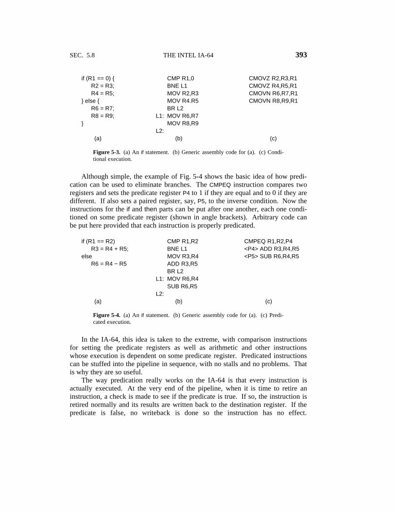
SEC. 5.8 THE INTEL IA-64 393
if (R1 == 0) { CMP R1,0 CMOVZ R2,R3,R1R2 = R3; BNE L1 CMOVZ R4,R5,R1R4 = R5; MOV R2,R3 CMOVN R6,R7,R1
} else { MOV R4.R5 CMOVN R8,R9,R1R6 = R7; BR L2R8 = R9; L1: MOV R6,R7
} MOV R8,R9L2:
(a) (b) (c)
Figure 5-3. (a) An if statement. (b) Generic assembly code for (a). (c) Condi-tional execution.
Although simple, the example of Fig. 5-4 shows the basic idea of how predi-cation can be used to eliminate branches. The CMPEQ instruction compares tworegisters and sets the predicate register P4 to 1 if they are equal and to 0 if they aredifferent. If also sets a paired register, say, P5, to the inverse condition. Now theinstructions for the if and then parts can be put after one another, each one condi-tioned on some predicate register (shown in angle brackets). Arbitrary code canbe put here provided that each instruction is properly predicated.
if (R1 == R2) CMP R1,R2 CMPEQ R1,R2,P4R3 = R4 + R5; BNE L1 <P4> ADD R3,R4,R5
else MOV R3,R4 <P5> SUB R6,R4,R5R6 = R4 − R5 ADD R3,R5
BR L2L1: MOV R6,R4
SUB R6,R5L2:
(a) (b) (c)
Figure 5-4. (a) An if statement. (b) Generic assembly code for (a). (c) Predi-cated execution.
In the IA-64, this idea is taken to the extreme, with comparison instructionsfor setting the predicate registers as well as arithmetic and other instructionswhose execution is dependent on some predicate register. Predicated instructionscan be stuffed into the pipeline in sequence, with no stalls and no problems. Thatis why they are so useful.
The way predication really works on the IA-64 is that every instruction isactually executed. At the very end of the pipeline, when it is time to retire aninstruction, a check is made to see if the predicate is true. If so, the instruction isretired normally and its results are written back to the destination register. If thepredicate is false, no writeback is done so the instruction has no effect.

394 THE INSTRUCTION SET ARCHITECTURE LEVEL CHAP. 5
Predication is discussed further in (Dulong, 1998).
5.8.4 Speculative Loads
Another feature of the IA-64 that speeds up execution is the presence ofspeculative LOADs. If a LOAD is speculative and it fails, instead of causing anexception, it just stops and a bit associated with the register to be loaded is setmarking the register as invalid. This is just the poison bit introduced in Chap. 4.If it turns out that the poisoned register is later used, the exception occurs at thattime; otherwise, it never happens.
The way speculation is normally used is for the compiler to hoist LOADs topositions before they are needed. By starting early, they may be finished beforethe results are needed. At the place where the compiler needs to use the registerjust loaded, it inserts a CHECK instruction. If the value is there, CHECK acts like aNOP and execution continues immediately. If the value is not there yet, the nextinstruction must stall. If an exception occurred and the poison bit is on, the pend-ing exception occurs at that point.
In summary, a machine implementing the the IA-64 architecture gets its speedfrom several sources. At the core is a state-of-the-art pipelined, load/store, three-address RISC engine. In addition, IA-64 has a model of explicit parallelism thatrequires the compiler to figure out which instructions can be executed at the sametime without conflicts and group them together in bundles. In this way the CPUcan just blindly schedule a bundle without having to do any heavy thinking. Next,predication allows the statements in both branches of an if statement to be mergedtogether in a single stream, eliminating the conditional branch and thus the predic-tion of which way it will go. Finally, speculative LOADs make it possible to fetchoperands in advance, without penalty if it turns out later that they are not neededafter all.
5.8.5 Reality Check
If all of these things work as expected, the Merced will indeed be a powerfulmachine. However, some caveats are in order. First, such an advanced machinehas never been built before, certainly not for a mass market audience. Historyshows that the best laid plans of rodents and persons sometimes go awry for vari-ous reasons.
Second, compilers for IA-64 will have to be written. Writing a good compilerfor the IA-64 architecture will not be easy. In addition, for the past 30 years, theholy grail of research in parallel programming has been the automatic extractionof parallelism from sequential programs. This work has not been very successful.If a program has little inherent parallelism or the compiler cannot extract it, theIA-64 bundles will all be short, with little gain.

SEC. 5.8 THE INTEL IA-64 395
Third, all of the above assumes the operating system is fully 64 bit. Windows95 and Windows 98 certainly are not and probably never will be. This means thateveryone will have to switch to Windows NT or some flavor of UNIX. This transi-tion may not be painless. After all, 10 years after the 32-bit 386 was introduced,Windows 95 still contained a large amount of 16-bit code, and it never used thesegmentation hardware that has been in all Intel CPUs for over a decade (segmen-tation will be discussed in Chap. 6). How long it will take for the operating sys-tems to become fully 64 bit is not known.
Fourth, many people will judge the IA-64 by how well it runs old 16-bit MS-
DOS games. When the Pentium Pro came out, it got a lot of bad press because itran old 16-bit programs no faster than the regular Pentium. Since old 16-bit (oreven 32-bit) programs will not even use the new features of IA-64 CPUs, all thepredicate registers in the world will not help them. To see any improvement, peo-ple will have to buy upgrades of all their software compiled with new IA-64-modecompilers. Many of them will balk at the expense.
Last, there may be alternatives from other vendors (including Intel) that alsoprovide high performance using more conventional RISC architectures, possiblywith more conditional instructions, essentially a weaker form of predication. Fas-ter versions of the Pentium II line itself will also be a serious competitor to theIA-64. It is likely that many years will pass before the IA-64 has the kind ofmarket dominance (if ever) that the IA-32 has now.

6THE OPERATING SYSTEM
MACHINE LEVEL
1

Level 1
Level 2
Level 3 Operating system machine level
Microarchitecture level
Operating system
Instruction set architecture level
Microprogram or hardware
Figure 6-1. Positioning of the operating system machine level.

Mapping
Address space
Address
8191
4096
0
4095
0
4K Mainmemory
Figure 6-2. A mapping in which virtual addresses 4096 to8191 are mapped onto main memory addresses 0 to 4095.

(a) (b)
Page Virtual addresses
15
14
13
12
11
10
9
8
7
6
5
4
3
2
1
0
61440 – 65535
57344 – 61439
53248 – 57343
49152 – 53247
45056 – 49151
40960 – 45055
36864 – 40959
32768 – 36863
28672 – 32767
24576 – 28671
20480 – 24575
16384 – 20479
12288 – 16383
8192 – 12287
4096 – 8191
0 – 4095
7
6
5
4
3
2
1
0
Pageframe
Bottom 32K ofmain memory
Physical addresses
28672 – 32767
24576 – 28671
20480 – 24575
16384 – 20479
12288 – 16383
8192 – 12287
4096 – 8191
0 – 4095
Figure 6-3. (a) The first 64K of virtual address space dividedinto 16 pages, with each page being 4K. (b) A 32K mainmemory divided up into eight page frames of 4K each.
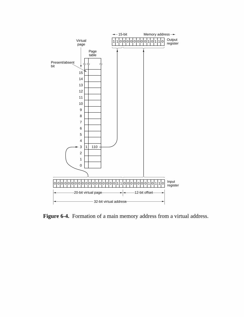
Present/absentbit
Virtualpage
Pagetable
15-bit
1
Memory address
Outputregister
1 110
15
14
13
12
11
10
9
8
7
6
5
4
3
2
1
0
1 0 0 0 0 0 0 0 0 1 0 1 1 0
0 0 0 0 0 0 0 0 0 0 0 0 0 0 0 0 0 0 1 1 0 0 0 0 0 0 0 1 0 1 1 0 Inputregister
20-bit virtual page 12-bit offset
32-bit virtual address
Figure 6-4. Formation of a main memory address from a virtual address.

Page table
Pageframe
0
1
0
0
1
0
0
1
0
1
1
0
1
0
1
1
0
4
0
0
5
0
0
3
0
7
6
0
2
0
0
1
Main memoryPageframe
1 = Present in main memory0 = Absent from main memory
7
6
5
4
3
2
1
0
Virtual page 6
Virtual page 5
Virtual page 11
Virtual page 14
Virtual page 8
Virtual page 3
Virtual page 0
Virtual page 1
Virtualpage
15
14
13
12
11
10
9
8
7
6
5
4
3
2
1
0
Figure 6-5. A possible mapping of the first 16 virtual pagesonto a main memory with eight page frames.

(a)
Virtual page 7
Virtual page 6
Virtual page 5
Virtual page 4
Virtual page 3
Virtual page 2
Virtual page 1
Virtual page 0
(b)
Virtual page 7
Virtual page 6
Virtual page 5
Virtual page 4
Virtual page 3
Virtual page 2
Virtual page 1
Virtual page 8
(c)
Virtual page 7
Virtual page 6
Virtual page 5
Virtual page 4
Virtual page 3
Virtual page 2
Virtual page 0
Virtual page 8
Figure 6-6. Failure of the LRU algorithm.

Virtual address space
Currently usedCall
stack
Constanttable
Symboltable
Address spaceallocated to thecall stack
Parsetree
Sourcetext
Free
Figure 6-7. In a one-dimensional address space with growingtables, one table may bump into another.
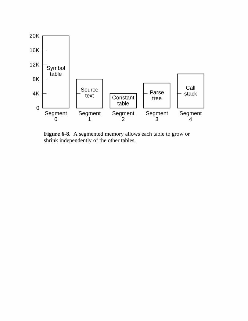
Segment0
Symboltable
Constanttable
CallstackParse
tree
20K
16K
12K
8K
4K
0Segment
1
Sourcetext
Segment2
Segment3
Segment4
Figure 6-8. A segmented memory allows each table to grow orshrink independently of the other tables.
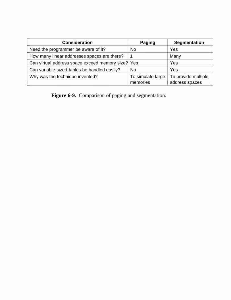
2222222222222222222222222222222222222222222222222222222222222222222222222222222222Consideration Paging Segmentation2222222222222222222222222222222222222222222222222222222222222222222222222222222222
Need the programmer be aware of it? No Yes2222222222222222222222222222222222222222222222222222222222222222222222222222222222How many linear addresses spaces are there? 1 Many2222222222222222222222222222222222222222222222222222222222222222222222222222222222Can virtual address space exceed memory size? Yes Yes2222222222222222222222222222222222222222222222222222222222222222222222222222222222Can variable-sized tables be handled easily? No Yes2222222222222222222222222222222222222222222222222222222222222222222222222222222222Why was the technique invented? To simulate large
memoriesTo provide multipleaddress spaces222222222222222222222222222222222222222222222222222222222222222222222222222222222211
111111111
11111111111
11111111111
11111111111
Figure 6-9. Comparison of paging and segmentation.

����������������
����������� ��� ���
�� �����
�����������������
����
Segment 1(8K)
(a)
Segment 3(8K)
Segment 3(8K)
Segment 4(7K)
Segment 4(7K)
Segment 3(8K)
Segment 2(5K)
Segment 0(4K)
(b)
Segment 7(5K)
Segment 0(4K)
(c) (d) (e)
Segment 2(5K)
Segment 7(5K)
Segment 0(4K)
Segment 2(5K)
Segment 5(4K)
Segment 7(5K)
Segment 0(4K)
Segment 2(5K)
Segment 6(4K)
Segment 5(4K)
Segment 7(5K)
Segment 0(4K)
Segment 6(4K)
Segment 5(4K)
Segment 2(5K)
10K
(4K)
(3K)(3K)
(3K) (3K)(3K)
Figure 6-10. (a)-(d) Development of external fragmentation(e) Removal of the external fragmentation by compaction.
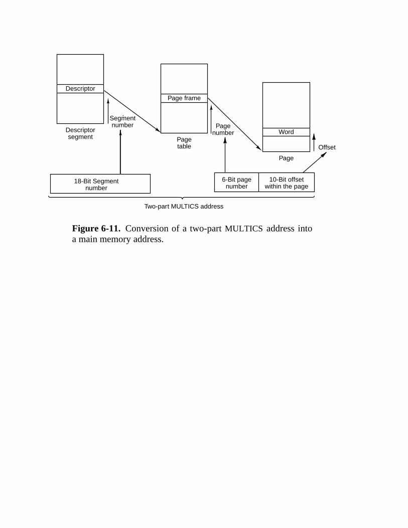
18-Bit Segmentnumber
Segmentnumber
Descriptor
Descriptorsegment
Pagenumber
Page frame
Pagetable Offset
Word
Page
6-Bit pagenumber
10-Bit offsetwithin the page
Two-part MULTICS address
Figure 6-11. Conversion of a two-part MULTICS address intoa main memory address.

Bits 13 1 2
INDEX
0 = GDT1 = LDT Privilege level (0-3)
Figure 6-12. A Pentium II selector.
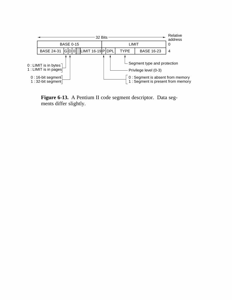
Relativeaddress0
4
BASE 0-15 LIMIT
BASE 24-31 G D 0 LIMIT 16-19 P DPL TYPE BASE 16-23
0 : LIMIT is in bytes1 : LIMIT is in pages
0 : 16-bit segment1 : 32-bit segment
Segment type and protection
Privilege level (0-3)
0 : Segment is absent from memory1 : Segment is present from memory
32 Bits
Figure 6-13. A Pentium II code segment descriptor. Data seg-ments differ slightly.

Selector
Descriptor
Base address
Limit
Other fields
32-bit linear address
Offset
+
Figure 6-14. Conversion of a (selector, offset) pair to a linear address.

Bits 10 10 12Linear address
DIR PAGE OFF
Page directory Page table Page frame
Word selected
(b)
(a)
DIR PAGEOFF
Figure 6-15. Mapping of a linear address onto a physical address.

Kernel
0
1
2
3
Level
Possible uses ofthe levels
System calls
Shared libraries
User programs
Figure 6-16. Protection on the Pentium II.
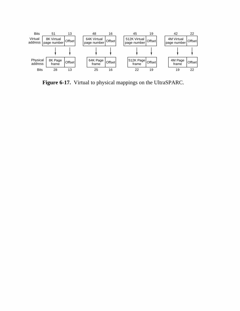
45 19
512K Virtualpage number Offset
22 19
512K Pageframe Offset
48 16
64K Virtualpage number Offset
25
64K Pageframe
16
Offset
Bits
Virtualaddress
51 13
8K Virtualpage number Offset
Bits
Physicaladdress
28
8K Pageframe
13
Offset
42 22
4M Virtualpage number Offset
22
Offset
19
4M Pageframe
Figure 6-17. Virtual to physical mappings on the UltraSPARC.

ValidPhysical
page
Virtualpage
Flags
(a)
TLB (MMU hardware)
Context
ValidPhysical
page
Virtualpagetag
Flags
(b)
(c)
Format isentirely
defined bythe operating
system
Translation table(Operating system)
TSB (MMU + sofware)
Context
Entry 0 is sharedby all virtual pagesending in 0…0000 Entry 1 is shared
by all virtual pagesending in 0…0001
Figure 6-18. Data structures used in translating virtual ad-dresses on the UltraSPARC. (a) TLB. (b) TSB. (c) Translationtable.

(a)
Logicalrecordnumber
Next logicalrecord to beread
Main memory
BufferLogicalrecord 18
15
14
16
17
18
19
20
21
22
23
24
25
(b)
1 logicalrecord
Next logicalrecord to beread
Main memory
BufferLogicalrecord 19
16
15
17
18
19
20
21
22
23
24
25
26
Figure 6-19. Reading a file consisting of logical records. (a)Before reading record 19. (b) After reading record 19.

Sector 11
Sector1
(a)
Sector 0
Read/writehead
Directionof diskrotation
120 13
14
1
2
3
456
7
8
910
11
Sector 11
Sector1
(b)
Sector 0
Read/writehead
Directionof diskrotation
4
7
10
2
Track 4
Track 03
5
60
12
11
14 13
9
1
8
Figure 6-20. Disk allocation strategies. (a) A file in consecu-tive sectors. (b) A file not in consecutive sectors.

(a)
(b)
Sector
00101
00001
00101
00010
00010
00110
10010
00010
00010
00000
01000
00001
0
01234
Track 1 2 3 4 65 7 8 9 10 11
Track Sector Number ofsectorsin hole
0011222334
06011137093
56101135338
Figure 6-21. Two ways of keeping track of available sectors.(a) A free list. (b) A bit map.
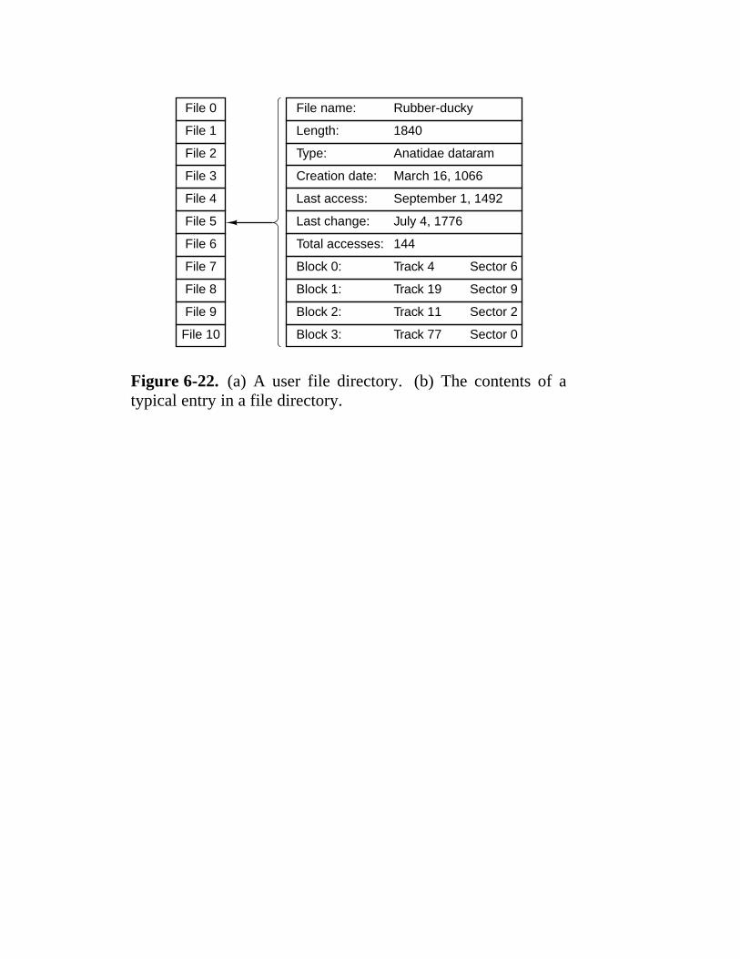
File 0
File 1
File 2
File 3
File 4
File 5
File 6
File 7
File 8
File 9
File 10
File name: Rubber-ducky
Length:
Type:
Creation date:
Last access:
Last change:
Total accesses:
Block 0:
Block 1:
Block 2:
Block 3:
1840
Anatidae dataram
March 16, 1066
September 1, 1492
July 4, 1776
144
Track 4
Track 19
Track 11
Track 77
Sector 6
Sector 9
Sector 2
Sector 0
Figure 6-22. (a) A user file directory. (b) The contents of atypical entry in a file directory.

(b)
Time
Process 3
Process 2
Process 1
Process 3
Process 2
Process 1
Process 3 waiting for CPU
Process 1 running
(a)
Time
Figure 6-23. (a) True parallel processing with multiple CPUs.(b) Parallel processing simulated by switching one CPU amongthree processes.

(a)
In,out
(b)Out
In
(c)
Out
In
(d)
Out
In
(e)
Out
In
(f)
In
Out
Figure 6-24. Use of a circular buffer.

public class m {final public static int BUF3SIZE = 100; // buffer runs from 0 to 99final public static long MAX3PRIME = 100000000000L; // stop herepublic static int in = 0, out = 0; // pointers to the datapublic static long buffer[ ] = new long[BUF3SIZE];// primes stored herepublic static producer p; // name of the producerpublic static consumer c; // name of the consumer
public static void main(String args[ ]) { // main classp = new producer( ); // create the producerc = new consumer( ); // create the consumerp.start( ); // start the producerc.start( ); // start the consumer
}
// This is a utility function for circularly incrementing in and outpublic static int next(int k) {if (k < BUF3SIZE − 1) return(k+1); else return(0);}
}
class producer extends Thread { // producer classpublic void run( ) { // producer code
long prime = 2; // scratch variable
while (prime < m.MAX3PRIME) {prime = next3prime(prime); // statement P1if (m.next(m.in) == m.out) suspend( ); // statement P2m.buffer[m.in] = prime; // statement P3m.in = m.next(m.in); // statement P4if (m.next(m.out) == m.in) m.c.resume( ); // statement P5
}}
private long next3prime(long prime){ ... } // function that computes next prime}
class consumer extends Thread { // consumer classpublic void run( ) { // consumer code
long emirp = 2; // scratch variable
while (emirp < m.MAX3PRIME) {if (m.in == m.out) suspend( ); // statement C1emirp = m.buffer[m.out]; // statement C2m.out = m.next(m.out); // statement C3if (m.out == m.next(m.next(m.in))) m.p.resume( );// statement C4System.out.println(emirp); // statement C5
}}
} Figure 6-25. Parallel processing with a fatal race condition.

(a)
100
In = 22
Out = 21 Prime
1 numberin buffer
Producer at P1consumer at C5
1 numberin buffer
1
Bufferempty
(b)
100
Producer at P1consumer at C1
In = Out = 22
1(c)
100
1
In = 23
Out = 22 Prime
Producer at P5sends wake upconsumer at C1
Figure 6-26. Failure of the producer-consumer communication mechanism.

22222222222222222222222222222222222222222222222222222222222222222222222222222Instr Semaphore = 0 Semaphore > 022222222222222222222222222222222222222222222222222222222222222222222222222222Up Semaphore=semaphore+1;
if the other process was halted attempting tocomplete a down instruction on this sema-phore, it may now complete the down andcontinue running
Semaphore=semaphore+1
22222222222222222222222222222222222222222222222222222222222222222222222222222Down Process halts until the other process ups this
semaphoreSemaphore=semaphore−1
2222222222222222222222222222222222222222222222222222222222222222222222222222211111111111
11111111111
11111111111
11111111111
Figure 6-27. The effect of a semaphore operation.

public class m {final public static int BUF3SIZE = 100; // buffer runs from 0 to 99final public static long MAX3PRIME = 100000000000L; // stop herepublic static int in = 0, out = 0; // pointers to the datapublic static long buffer[ ] = new long[BUF3SIZE];// primes stored herepublic static producer p; // name of the producerpublic static consumer c; // name of the consumerpublic static int filled = 0, available = 100; // semaphores
public static void main(String args[ ]) { // main classp = new producer( ); // create the producerc = new consumer( ); // create the consumerp.start( ); // start the producerc.start( ); // start the consumer
}
// This is a utility function for circularly incrementing in and outpublic static int next(int k) {if (k < BUF3SIZE − 1) return(k+1); else return(0);}
}
class producer extends Thread { // producer classnative void up(int s); native void down(int s); // methods on semaphorespublic void run( ) { // producer code
long prime = 2; // scratch variable
while (prime < m.MAX3PRIME) {prime = next3prime(prime); // statement P1down(m.available); // statement P2m.buffer[m.in] = prime; // statement P3m.in = m.next(m.in); // statement P4up(m.filled); // statement P5
}}
private long next3prime(long prime){ ... } // function that computes next prime}
class consumer extends Thread { // consumer classnative void up(int s); native void down(int s); // methods on semaphorespublic void run( ) { // consumer code
long emirp = 2; // scratch variable
while (emirp < m.MAX3PRIME) {down(m.filled); // statement C1emirp = m.buffer[m.out]; // statement C2m.out = m.next(m.out); // statement C3up(m.available); // statement C4System.out.println(emirp); // statement C5
}}
} Figure 6-28. Parallel processing using semaphores.

22222222222222222222222222222222222222222222222222222222222222222222222222222222222Category Some examples22222222222222222222222222222222222222222222222222222222222222222222222222222222222
File management Open, read, write, close, and lock files22222222222222222222222222222222222222222222222222222222222222222222222222222222222Directory management Create and delete directories; move files around22222222222222222222222222222222222222222222222222222222222222222222222222222222222Process management Spawn, terminate, trace, and signal processes22222222222222222222222222222222222222222222222222222222222222222222222222222222222Memory management Share memory among processes; protect pages22222222222222222222222222222222222222222222222222222222222222222222222222222222222Getting/setting parameters Get user, group, process ID; set priority22222222222222222222222222222222222222222222222222222222222222222222222222222222222Dates and times Set file access times; use interval timer; profile execution22222222222222222222222222222222222222222222222222222222222222222222222222222222222Networking Establish/accept connection; send/receive message22222222222222222222222222222222222222222222222222222222222222222222222222222222222Miscellaneous Enable accounting; manipulate disk quotas; reboot the system2222222222222222222222222222222222222222222222222222222222222222222222222222222222211111111111111
11111111111111
11111111111111
Figure 6-29. A rough breakdown of the UNIX system calls.
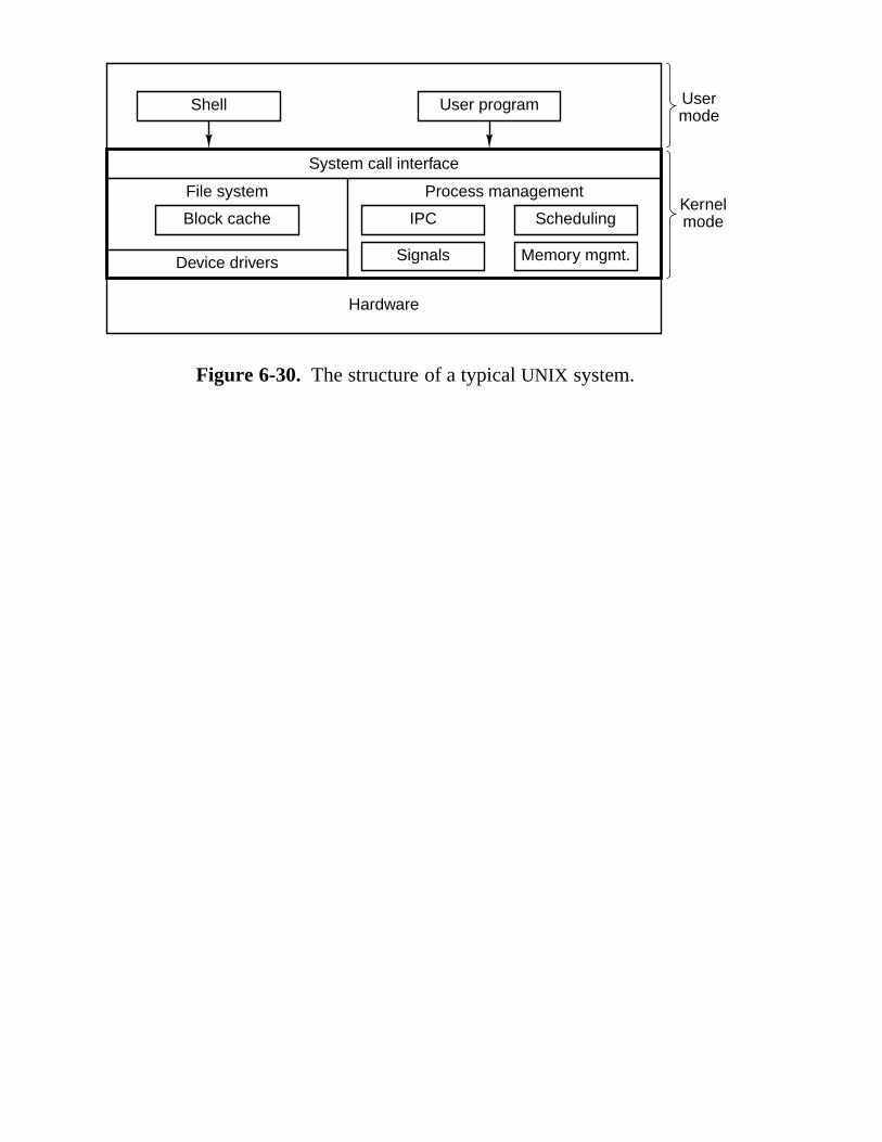
Shell User program
System call interface
File system Process management
Block cache IPC Scheduling
Hardware
Device drivers
Usermode
Kernelmode
Memory mgmt.Signals
Figure 6-30. The structure of a typical UNIX system.
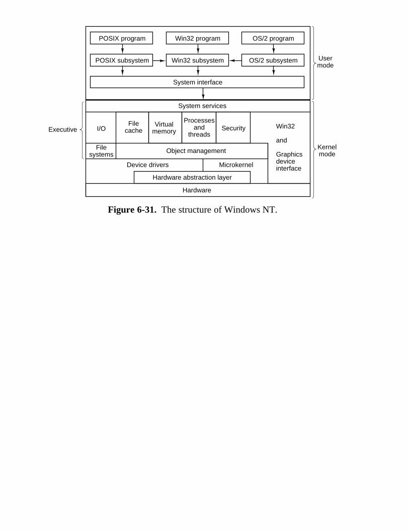
System services
Hardware
Usermode
Kernelmode
Executive I/O
Filesystems
Security Win32
and
Graphicsdeviceinterface
Object management
Hardware abstraction layer
POSIX program
POSIX subsystem
Win32 program
Win32 subsystem
OS/2 program
OS/2 subsystem
System interface
Virtualmemory
Device drivers Microkernel
Filecache
Processesand
threads
Figure 6-31. The structure of Windows NT.

22222222222222222222222222222222222222222222222222222222222222222222222222222Item Windows 95/98 NT 5.022222222222222222222222222222222222222222222222222222222222222222222222222222Win32 API? Yes Yes22222222222222222222222222222222222222222222222222222222222222222222222222222Full 32-bit system? No Yes22222222222222222222222222222222222222222222222222222222222222222222222222222Security? No Yes22222222222222222222222222222222222222222222222222222222222222222222222222222Protected file mappings? No Yes22222222222222222222222222222222222222222222222222222222222222222222222222222Sep. addr space for each MS-DOS program? No Yes22222222222222222222222222222222222222222222222222222222222222222222222222222Plug and play? Yes Yes22222222222222222222222222222222222222222222222222222222222222222222222222222Unicode? No Yes22222222222222222222222222222222222222222222222222222222222222222222222222222Runs on Intel 80x86 80x86, Alpha22222222222222222222222222222222222222222222222222222222222222222222222222222Multiprocessor support? No Yes22222222222222222222222222222222222222222222222222222222222222222222222222222Re-entrant code inside OS? No Yes22222222222222222222222222222222222222222222222222222222222222222222222222222Some critical OS data writable by user? Yes No22222222222222222222222222222222222222222222222222222222222222222222222222222111111111111111111
111111111111111111
111111111111111111
111111111111111111
Figure 6-32. Some differences between versions of Windows.

Address
0xFFFFFFFF
0Code
Data
Stack
Figure 6-33. The address space of a single UNIX process.

2222222222222222222222222222222222222222222222222222222222222222222222222222222API function Meaning2222222222222222222222222222222222222222222222222222222222222222222222222222222
VirtualAlloc Reserve or commit a region2222222222222222222222222222222222222222222222222222222222222222222222222222222VirtualFree Release or decommit a region2222222222222222222222222222222222222222222222222222222222222222222222222222222VirtualProtect Change the read/write/execute protection on a region2222222222222222222222222222222222222222222222222222222222222222222222222222222VirtualQuery Inquire about the status of a region2222222222222222222222222222222222222222222222222222222222222222222222222222222VirtualLock Make a region memory resident (i.e., disable paging for it)2222222222222222222222222222222222222222222222222222222222222222222222222222222VirtualUnlock Make a region pageable in the usual way2222222222222222222222222222222222222222222222222222222222222222222222222222222CreateFileMapping Create a file mapping object and (optionally) assign it a name2222222222222222222222222222222222222222222222222222222222222222222222222222222MapViewOfFile Map (part of) a file into the address space2222222222222222222222222222222222222222222222222222222222222222222222222222222UnmapViewOfFile Remove a mapped file from the address space2222222222222222222222222222222222222222222222222222222222222222222222222222222OpenFileMapping Open a previously created file mapping object222222222222222222222222222222222222222222222222222222222222222222222222222222211111111111111111
11111111111111111
11111111111111111
Figure 6-34. The principal API functions for managing virtualmemory in Windows NT.
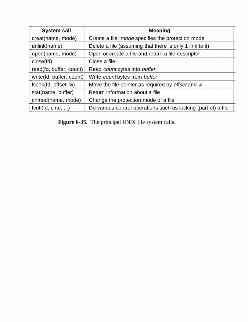
222222222222222222222222222222222222222222222222222222222222222222222222222222System call Meaning222222222222222222222222222222222222222222222222222222222222222222222222222222
creat(name, mode) Create a file; mode specifies the protection mode222222222222222222222222222222222222222222222222222222222222222222222222222222unlink(name) Delete a file (assuming that there is only 1 link to it)222222222222222222222222222222222222222222222222222222222222222222222222222222open(name, mode) Open or create a file and return a file descriptor222222222222222222222222222222222222222222222222222222222222222222222222222222close(fd) Close a file222222222222222222222222222222222222222222222222222222222222222222222222222222read(fd, buffer, count) Read count bytes into buffer222222222222222222222222222222222222222222222222222222222222222222222222222222write(fd, buffer, count) Write count bytes from buffer222222222222222222222222222222222222222222222222222222222222222222222222222222lseek(fd, offset, w) Move the file pointer as required by offset and w222222222222222222222222222222222222222222222222222222222222222222222222222222stat(name, buffer) Return information about a file222222222222222222222222222222222222222222222222222222222222222222222222222222chmod(name, mode) Change the protection mode of a file222222222222222222222222222222222222222222222222222222222222222222222222222222fcntl(fd, cmd, ...) Do various control operations such as locking (part of) a file22222222222222222222222222222222222222222222222222222222222222222222222222222211111111111111111
11111111111111111
11111111111111111
Figure 6-35. The principal UNIX file system calls.

// Open the file descriptorsinfd = open(′′data′′, 0);outfd = creat(′′newf′′, ProtectionBits);
// Copy loopdo {
count = read(infd, buffer, bytes);if (count > 0) write(outfd, buffer, count);
} while (count > 0);
// Close the filesclose(infd);close(outfd);
Figure 6-36. A program fragment for copying a file using theUNIX system calls. This fragment is in C because Java hidesthe low-level system calls and we are trying to expose them.

/usr/ast/bin
Data files
game 1
game 2
game 3
game 4
…
/usr/ast
bin
data
foo.c
…
/usr/jim
jotto
…
Root directory
bin
dev
lib
usr
…
/lib
…
/usr
ast
jim
…
/dev
…
/bin
…
Figure 6-37. Part of a typical UNIX directory system.

222222222222222222222222222222222222222222222222222222222222222222222222System call Meaning222222222222222222222222222222222222222222222222222222222222222222222222
mkdir(name, mode) Create a new directory222222222222222222222222222222222222222222222222222222222222222222222222rmdir(name) Delete an empty directory222222222222222222222222222222222222222222222222222222222222222222222222opendir(name) Open a directory for reading222222222222222222222222222222222222222222222222222222222222222222222222readdir(dirpointer) Read the next entry in a directory222222222222222222222222222222222222222222222222222222222222222222222222closedir(dirpointer) Close a directory222222222222222222222222222222222222222222222222222222222222222222222222chdir(dirname) Change working directory to dirname222222222222222222222222222222222222222222222222222222222222222222222222link(name1, name2) Create a directory entry name2 pointing to name1222222222222222222222222222222222222222222222222222222222222222222222222unlink(name) Remove name from its directory2222222222222222222222222222222222222222222222222222222222222222222222221111111111111
1111111111111
1111111111111
Figure 6-38. The principal UNIX directory management calls.
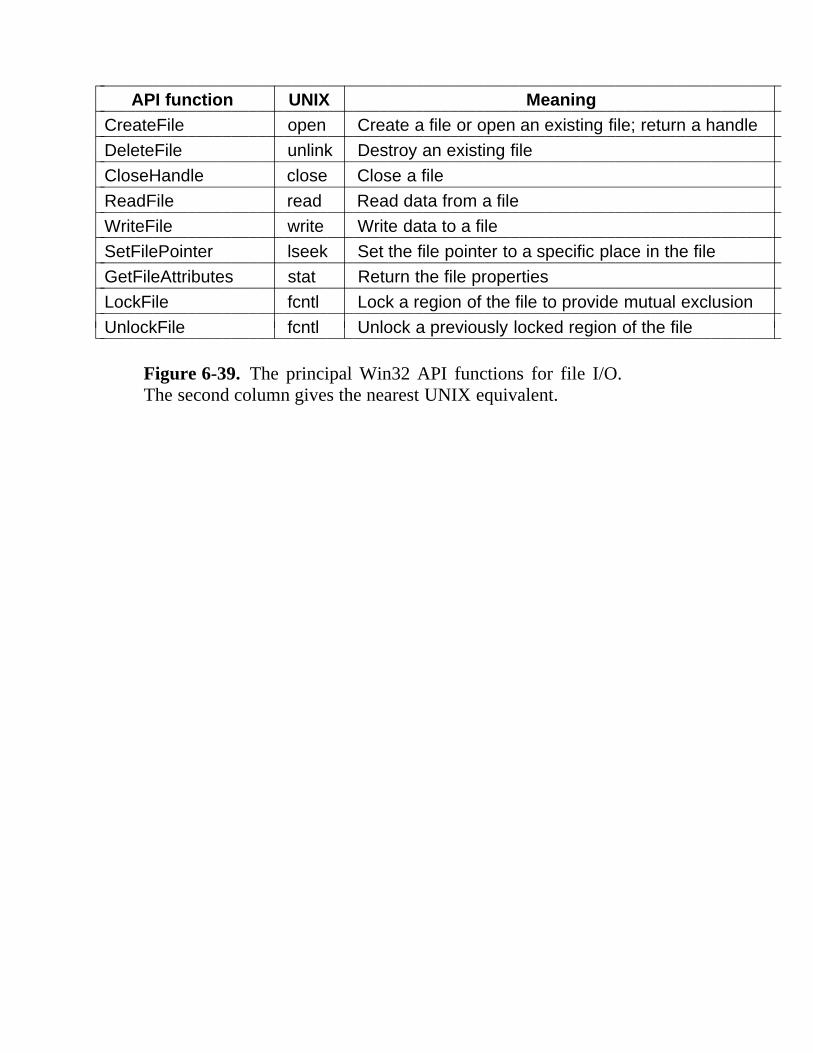
2222222222222222222222222222222222222222222222222222222222222222222222222222222API function UNIX Meaning2222222222222222222222222222222222222222222222222222222222222222222222222222222
CreateFile open Create a file or open an existing file; return a handle2222222222222222222222222222222222222222222222222222222222222222222222222222222DeleteFile unlink Destroy an existing file2222222222222222222222222222222222222222222222222222222222222222222222222222222CloseHandle close Close a file2222222222222222222222222222222222222222222222222222222222222222222222222222222ReadFile read Read data from a file2222222222222222222222222222222222222222222222222222222222222222222222222222222WriteFile write Write data to a file2222222222222222222222222222222222222222222222222222222222222222222222222222222SetFilePointer lseek Set the file pointer to a specific place in the file2222222222222222222222222222222222222222222222222222222222222222222222222222222GetFileAttributes stat Return the file properties2222222222222222222222222222222222222222222222222222222222222222222222222222222LockFile fcntl Lock a region of the file to provide mutual exclusion2222222222222222222222222222222222222222222222222222222222222222222222222222222UnlockFile fcntl Unlock a previously locked region of the file2222222222222222222222222222222222222222222222222222222222222222222222222222222111111111111111
111111111111111
111111111111111
111111111111111
Figure 6-39. The principal Win32 API functions for file I/O.The second column gives the nearest UNIX equivalent.

// Open files for input and output.inhandle = CreateFile( ′′data′′, GENERIC3READ, 0, NULL, OPEN3EXISTING, 0, NULL);outhandle = CreateFile(′′newf′′, GENERIC3WRITE, 0, NULL, CREATE3ALWAYS,
FILE3ATTRIBUTE3NORMAL, NULL);
// Copy the file.do {
s = ReadFile(inhandle, buffer, BUF3SIZE, &count, NULL);if (s > 0 && count > 0) WriteFile(outhandle, buffer, count, &ocnt, NULL);
while (s > 0 && count > 0);
// Close the files.CloseHandle(inhandle);CloseHandle(outhandle);
Figure 6-40. A program fragment for copying a file using theWindows NT API functions. This fragment is in C becauseJava hides the low-level system calls and we are trying to ex-pose them.

2222222222222222222222222222222222222222222222222222222222222222222222222222222API function UNIX Meaning2222222222222222222222222222222222222222222222222222222222222222222222222222222
CreateDirectory mkdir Create a new directory2222222222222222222222222222222222222222222222222222222222222222222222222222222RemoveDirectory rmdir Remove an empty directory2222222222222222222222222222222222222222222222222222222222222222222222222222222FindFirstFile opendir Initialize to start reading the entries in a directory2222222222222222222222222222222222222222222222222222222222222222222222222222222FindNextFile readdir Read the next directory entry2222222222222222222222222222222222222222222222222222222222222222222222222222222MoveFile Move a file from one directory to another2222222222222222222222222222222222222222222222222222222222222222222222222222222SetCurrentDirectory chdir Change the current working directory222222222222222222222222222222222222222222222222222222222222222222222222222222211111111111
11111111111
11111111111
11111111111
Figure 6-41. The principal Win32 API functions for directorymanagement. The second column gives the nearest UNIXequivalent, when one exists.

MFTheader
MFT entry for one file
Standardinformation
MS-DOSnameFile name Security Data
Masterfile
table
Figure 6-42. The Windows NT master file table.

Original process
Children of A
Grandchildren of AA A A
A
A A
Figure 6-43. A process tree in UNIX.

2222222222222222222222222222222222222222222222222222222222222222222222222222222Thread call Meaning2222222222222222222222222222222222222222222222222222222222222222222222222222222
pthread3create Create a new thread in the caller’s address space2222222222222222222222222222222222222222222222222222222222222222222222222222222pthread3exit Terminate the calling thread2222222222222222222222222222222222222222222222222222222222222222222222222222222pthread3join Wait for a thread to terminate2222222222222222222222222222222222222222222222222222222222222222222222222222222pthread3mutex3init Create a new mutex2222222222222222222222222222222222222222222222222222222222222222222222222222222pthread3mutex3destroy Destroy a mutex2222222222222222222222222222222222222222222222222222222222222222222222222222222pthread3mutex3lock Lock a mutex2222222222222222222222222222222222222222222222222222222222222222222222222222222pthread3mutex3unlock Unlock a mutex2222222222222222222222222222222222222222222222222222222222222222222222222222222pthread3cond3init Create a condition variable2222222222222222222222222222222222222222222222222222222222222222222222222222222pthread3cond3destroy Destroy a condition variable2222222222222222222222222222222222222222222222222222222222222222222222222222222pthread3cond3wait Wait on a condition variable2222222222222222222222222222222222222222222222222222222222222222222222222222222pthread3cond3signal Release one thread waiting on a condition variable2222222222222222222222222222222222222222222222222222222222222222222222222222222111111111111111111
111111111111111111
111111111111111111
Figure 6-44. The principal POSIX thread calls.

446 THE OPERATING SYSTEM MACHINE LEVEL CHAP. 6
6.4 EXAMPLE OPERATING SYSTEMS
In this section we will continue discussing our example systems, the PentiumII and the UltraSPARC. For each one we will look at an operating system used onthat processor. For the Pentium II we will use Windows NT (called NT for shortbelow); for the UltraSPARC II we will use UNIX. Since UNIX is simpler and inmany ways more elegant, we will begin with it. Also, UNIX was designed andimplemented first and had a major influence on NT, so this order makes moresense than the reverse.
6.4.1 Introduction
In this section we will give a brief introduction to our two example operatingsystems, UNIX and NT, focusing on the history, structure, and system calls.
UNIX
UNIX was developed at Bell Labs in the early 1970s. The first version waswritten by Ken Thompson in assembler for the PDP-7 minicomputer. This wassoon followed by a version for the PDP-11, written in a new language called Cthat was devised and implemented by Dennis Ritchie. In 1974, Ritchie andThompson published a landmark paper about UNIX (Ritchie and Thompson, 1974).For the work described in this paper they were later given the prestigious ACMTuring Award (Ritchie, 1984; Thompson, 1984). The publication of this paperstimulated many universities to ask Bell Labs for a copy of UNIX. Since BellLabs’ parent company, AT&T, was a regulated monopoly at the time and was notpermitted to be in the computer business, it had no objection to licensing UNIX touniversities for a modest fee.
In one of those coincidences that often shape history, the PDP-11 was thecomputer of choice at nearly all university computer science departments, and theoperating systems that came with the PDP-11 were widely regarded as beingdreadful by professors and students alike. UNIX quickly filled the void, not in theleast because it was supplied with the complete source code, so people could, anddid, tinker with it endlessly.
One of the many universities that acquired UNIX early on was the Universityof California at Berkeley. Because the complete source code was available,Berkeley was able to modify the system substantially. Foremost among thechanges was a port to the VAX minicomputer and the addition of paged virtualmemory, the extension of file names from 14 characters to 255 characters, and theinclusion of the TCP/IP networking protocol, which is now used on the Internet(largely due to the fact that it was in Berkeley UNIX).
While Berkeley was making all these changes, AT&T itself continued todevelop UNIX, leading to System III in 1982 and then System V in 1984. By the

SEC. 6.4 EXAMPLE OPERATING SYSTEMS 447
late 1980s, two different, and quite incompatible, versions of UNIX were inwidespread use: Berkeley UNIX and System V. This split in the UNIX world,together with the fact that there were no standards for binary program formats,greatly inhibited the commercial success of UNIX because it was impossible forsoftware vendors to write and package UNIX programs with the expectation thatthey would run on any UNIX system (as was routinely done with MS-DOS). Aftermuch bickering, a standard called POSIX (Portable Operating System-IX) wascreated by the IEEE Standards Board. POSIX is also known by its IEEE Standardsnumber, P1003. It later became an International Standard.
The POSIX standard is divided into many parts, each covering a different areaof UNIX. The first part, P1003.1, defines the system calls; the second part,P1003.2, defines the basic utility programs, and so on. The P1003.1 standarddefines about 60 system calls that all conformant systems must support. These arethe basic calls for reading and writing files, creating new processes, and so on.Nearly all UNIX systems now support the P1003.1 system calls. However manyUNIX systems also support extra system calls, especially those defined by SystemV and/or those in Berkeley UNIX. Typically these add up to perhaps 100 systemcalls to the POSIX set. The operating system for the UltraSPARC II is based onSystem V and is called Solaris. It also supports many of the Berkeley systemcalls.
A rough breakdown of the Solaris system calls by category is given in Fig. 6-1. The file and directory management system calls are largest and the mostimportant categories. Most of these come from P1003.1. A relatively large frac-tion of the others are derived from System V.22222222222222222222222222222222222222222222222222222222222222222222222222222222222
Category Some examples22222222222222222222222222222222222222222222222222222222222222222222222222222222222File management Open, read, write, close, and lock files22222222222222222222222222222222222222222222222222222222222222222222222222222222222Directory management Create and delete directories; move files around22222222222222222222222222222222222222222222222222222222222222222222222222222222222Process management Spawn, terminate, trace, and signal processes22222222222222222222222222222222222222222222222222222222222222222222222222222222222Memory management Share memory among processes; protect pages22222222222222222222222222222222222222222222222222222222222222222222222222222222222Getting/setting parameters Get user, group, process ID; set priority22222222222222222222222222222222222222222222222222222222222222222222222222222222222Dates and times Set file access times; use interval timer; profile execution22222222222222222222222222222222222222222222222222222222222222222222222222222222222Networking Establish/accept connection; send/receive message22222222222222222222222222222222222222222222222222222222222222222222222222222222222Miscellaneous Enable accounting; manipulate disk quotas; reboot the system2222222222222222222222222222222222222222222222222222222222222222222222222222222222211
1111111111111
111111111111111
111111111111111
Figure 6-1. A rough breakdown of the UNIX system calls.
One area that is largely due to Berkeley UNIX rather than System V is net-working. Berkeley invented the concept of a socket, which is the endpoint of anetwork connection. The four-pin wall plugs to which telephones can be con-nected served as the model for this concept. It is possible for a UNIX process tocreate a socket, attach to it, and establish a connection to a socket on a distant

448 THE OPERATING SYSTEM MACHINE LEVEL CHAP. 6
machine. Over this connection it can then exchange data in both directions, typi-cally using the TCP/IP protocol. Since networking technology has been in UNIX
for decades and is very stable and mature, a substantial fraction of the servers onthe Internet run UNIX.
Since there are many implementations of UNIX, it is difficult to say muchabout the structure of the operating system since every one is somewhat differentfrom all the others. However, in general, Fig. 6-2 applies to most of them. At thebottom, there is a layer of device drivers that shield the file system from the barehardware. Originally, each device driver was written as an independent entity,separate from all the others. This arrangement led to a lot of duplicated effort,since many drivers must deal with flow control, error handling, priorities, separat-ing data from control, and so on. This observation led Dennis Ritchie to developa framework called streams for writing drivers in a modular way. With a stream,it is possible to establish a two-way connection from a user process to a hardwaredevice and to insert one or more modules along the path. The user process pushesdata into the stream, which then is processed or transformed by each module untilit gets to the hardware. The inverse processing occurs for incoming data.
Shell User program
System call interface
File system Process management
Block cache IPC Scheduling
Hardware
Device drivers
Usermode
Kernelmode
Memory mgmt.Signals
Figure 6-2. The structure of a typical UNIX system.
On top of the device drivers comes the file system. It manages file names,directories, disk block allocation, protection, and much more. Part of the file sys-tem is a block cache, for holding the blocks most recently read in from disk, incase they are needed again soon. A variety of file systems have been used overthe years, including the Berkeley fast file system (McKusick et al., 1984), andlog-structured file systems (Rosenblum and Ousterhout, 1991; and Seltzer et al.,1993).
The other part of the UNIX kernel is the process management portion. Amongits various other functions, it handles IPC (InterProcess Communication), whichallows processes to communicate with one another and synchronize to avoid raceconditions. A variety of mechanisms are provided. The process management

SEC. 6.4 EXAMPLE OPERATING SYSTEMS 449
code also handles process scheduling, which is based on priorities. Signals, whichare a form of (asynchronous) software interrupt, are also managed here. Finally,memory management is done here as well. Most UNIX systems support demand-paged virtual memory, sometimes with a few extra features, such as the ability ofmultiple processes to share common regions of address space.
From its inception, UNIX has tried to be a small system, in order to enhancereliability and performance. The first versions of UNIX were entirely text-based,using terminals that could display 24 or 25 lines of 80 ASCII characters. The userinterface was handled by a user-level program called the shell, which offered acommand line interface. Since the shell was not part of the kernel, adding newshells to UNIX was easy, and over time a number of increasingly sophisticatedones were invented.
Later on, when graphics terminals came into existence, a windowing systemfor UNIX, called X Windows, was developed at M.I.T. Still later, a full-fledgedGUI (Graphical User Interface), called Motif, was put on top of X Windows.In keeping with the UNIX philosophy of having a small kernel, nearly all the codeof X Windows and Motif runs in user mode, outside the kernel.
Windows NT
When the original IBM PC was launched in 1981, it came equipped with a16-bit real-mode, single-user, command-line oriented operating system calledMS-DOS 1.0. This operating system consisted of 8 KB of memory resident code.Two years later, a much more powerful 24-KB system, MS-DOS 2.0, appeared. Itcontained a command line processor (shell), with a number of features borrowedfrom UNIX. When IBM released the 286-based PC/AT in 1984, it came equippedwith MS-DOS 3.0, by now 36 KB. Over the years, MS-DOS continued to acquirenew features, but it was still a command-line oriented system.
Inspired by the success of the Apple Macintosh, Microsoft decided to giveMS-DOS a graphical user interface that it called Windows. The first three versionsof Windows, culminating in Windows 3.x, were not true operating systems, butgraphical user interfaces on top of MS-DOS, which was still in control of themachine. All programs ran in the same address space and a bug in any one ofthem could bring the whole system to a grinding halt.
The release of Windows 95 in 1995 still did not eliminate MS-DOS, although itintroduced a new version, 7.0. Together, Windows 95 and MS-DOS 7.0 containedmost of the features of a full-blown operating system, including virtual memory,process management, and multiprogramming. However, Windows 95 was not afull 32-bit program. It contained large chunks of old 16-bit code (as well as some32-bit code) and still used the MS-DOS file system, with nearly all its limitations.The only major change to the file system was the addition of long file names inplace of the 8 + 3 character file names allowed in MS-DOS.
Even with the release of Windows 98 in 1998, MS-DOS was still there (now

450 THE OPERATING SYSTEM MACHINE LEVEL CHAP. 6
called version 7.1) and running 16-bit code. Although a bit more functionalitymigrated from the MS-DOS part to the Windows part, and a disk layout suitable forlarger disks was now standard, under the hood, Windows 98 was not very dif-ferent from Windows 95. The main difference was the user interface, whichintegrated the desktop, the Internet, and television more closely. It was preciselythis integration that attracted the attention of the U.S. Dept. of Justice, which thensued Microsoft claiming that it was an illegal monopoly.
While all these developments were going on, Microsoft was also busy with acompletely new 32-bit operating system being written from the ground up. Thisnew system was called Windows New Technology, or Windows NT. It was ini-tially hyped as the replacement for all other operating systems for Intel-basedPCs, but it was somewhat slow to catch on and was later redirected to the upperend of the market, where it found a niche. It is gradually becoming more popularat the low end as well.
NT is sold in two versions: server and workstation. These two versions arenearly identical and are generated from the same source code. The server versionis intended for machines that run as LAN-based file and print servers and hasmore elaborate management features than the workstation version, which isintended for desktop computing for a single user. The server version has a variant(enterprise) intended for large sites. The various versions are tuned differently,each one optimized for its expected environment. Other than these minor differ-ences, all the versions are essentially the same. In fact, nearly all the executablefiles are identical for all versions. NT itself discovers which version it is by look-ing at a variable in an internal data structure (the registry). Users are forbidden bythe license from changing this variable and thus converting the (inexpensive)workstation version into the (much more expensive) server or enterprise versions.We will not make any further distinction between these versions.
MS-DOS and all previous versions of Windows were single-user systems. NT,however, supports multiprogramming, so several users can work on the samemachine at the same time. For example, a network server may have multipleusers logged in simultaneously over a network, each accessing its own files in aprotected way.
NT is a true 32-bit multiprogramming operating system. It supports multipleuser processes, each of which has a full 32-bit demand-paged virtual addressspace. In addition, the system itself is written as 32-bit code everywhere.
One of NT’s original improvements over Windows 95 was its modular struc-ture. It consisted of a moderately small kernel that ran in kernel mode, plus anumber of server processes that ran in user mode. User processes interacted withthe server processes using the client-server model: a client sent a request messageto a server, and the server did the work and returned the result to the client via asecond message. This modular structure made it easier to port it to several com-puters besides the Intel line, including the DEC Alpha, IBM PowerPC, and SGIMIPS. However, for performance reasons, starting with NT 4.0, pretty much all of

SEC. 6.4 EXAMPLE OPERATING SYSTEMS 451
the system was put back into the kernel.One could go on for a long time both about how NT is structured internally
and what its system call interface is like. Since our primary interest here is thevirtual machine presented by various operating systems (i.e., the system calls), wewill give a brief summary of the system structure and then move on to the systemcall interface.
The structure of NT is illustrated in Fig. 6-3. It consists of a number ofmodules that are structured in layers and work together to implement the operat-ing system. Each module has some particular function and a well-defined inter-face to the other modules. Nearly all the modules are written in C, although partof the graphics device interface is written in C++ and a tiny bit of the lowestlayers are written in assembly language.
At the bottom is a thin layer called the hardware abstraction layer. Its jobis to present the rest of the operating system with abstract hardware devices,devoid of the warts and idiosyncracies with which real hardware is so richlyendowed. Among the devices modeled are off-chip caches, timers, I/O buses,interrupt controllers, and DMA controllers. By exposing these to the rest of theoperating system in idealized form, it becomes easier to port NT to other hardwareplatforms, since most of the modifications required are concentrated in one place.
System services
Hardware
Usermode
Kernelmode
Executive I/O
Filesystems
Security Win32
and
Graphicsdeviceinterface
Object management
Hardware abstraction layer
POSIX program
POSIX subsystem
Win32 program
Win32 subsystem
OS/2 program
OS/2 subsystem
System interface
Virtualmemory
Device drivers Microkernel
Filecache
Processesand
threads
Figure 6-3. The structure of Windows NT.
Above the hardware abstraction layer is a layer containing the microkernel.and the device drivers. The microkernel and all the device drivers have directaccess to the hardware when needed, as they contain hardware-dependent code.
The microkernel supports the primitive kernel objects, interrupt, trap, and

452 THE OPERATING SYSTEM MACHINE LEVEL CHAP. 6
exception handling, process scheduling and synchronization, multiprocessor syn-chronization, and time management. The purpose of this layer is to make the restof the operating system completely independent of the hardware, and thus highlyportable. The microkernel is permanently resident in main memory and is notpreemptable, although it can temporarily give up control to service I/O interrupts.
Each device driver can control one or more I/O devices, but a device drivercan also do things not related to a specific device, such as encrypting a datastream or even just providing access to kernel data structures. Since users caninstall new device drivers, they have the power to affect the kernel and corrupt thesystem. For this reason, drivers must be written with great care.
Above the microkernel and device drivers is the upper portion of the operatingsystem, called the executive. The executive is architecture independent and canbe ported to new machines with relatively little effort. It consists of three layers.
The lowest layer contains the file systems and the object manager. The filesystems support the use of files and directories The object manager handlesobjects known to the kernel. These include processes, threads (lightweightprocesses within an address space), files, directories, semaphores, I/O devices,timers, and many others. It also manages a namespace in which newly createdobjects can be placed so they can be referred to later.
The next layer consists of six major parts, as shown in Fig. 6-3. The I/Omanager provides a framework for managing I/O devices and provides genericI/O services. It uses the services of the file system, which in turn uses the devicedrivers, as well as the services of the object manager.
The cache manager keeps the most recently used disk blocks in memory tospeed up access to them in the (likely) event that they are needed again. Its job isto figure out which blocks are probably going to be needed again and which onesare not. It is possible to configure NT with multiple file systems, in which case thecache manager works for all of them, so each one does not have to do its owncache management. When a block is needed, the cache manager is asked to sup-ply it. If it does not have the block, the cache manager calls upon the appropriatefile system to get it. Since files can be mapped into processes’ address spaces, thecache manager must interact with the virtual memory manager to provide thenecessary consistency.
The virtual memory manager implements NT’s demand-paged virtualmemory architecture. It manages the mapping of virtual pages onto physical pageframes. It thereby enforces the protection rules that restrict each process to onlyaccess those pages belonging to its address space and not to other processes,address spaces (except under special circumstances). It also handles certain sys-tem calls that relate to virtual memory.
The process and thread manager handles processes and threads, includingtheir creation and destruction. It is concerned about the mechanisms used tomanage them, rather than policies about how they are used.
The security manager enforces NT’s elaborate security mechanism, which

SEC. 6.4 EXAMPLE OPERATING SYSTEMS 453
meets the U.S. Dept. of Defense’s Orange Book C2 requirements. The OrangeBook specifies a large number of rules that a conforming system must meet, start-ing with authenticated login through how access control is handled to the fact thatvirtual pages must be zeroed out before being reused.
The graphics device interface handles image management for the monitorand printers. It provides system calls to allow user programs to write on the moni-tor or printers in a device-independent way. It also contains the window managerand hardware device drivers. In versions of NT prior to NT 4.0, it was in user spacebut the performance was disappointing, so Microsoft moved it into the kernel tospeed it up. The Win32 module also handles most of the system calls. It, too,was originally in user space but were also moved to the kernel to improve perfor-mance.
On the top of the executive is a thin layer called system services. Its functionis to provide an interface to the executive. It accepts the true NT system calls andcalls other parts of the executive to have them executed.
Outside the kernel are the user programs and the environmental subsystems.The environmental subsystems are provided because user programs are notencouraged to make system calls directly (although they are technically capableof it). Instead, each environmental subsystem exports a (different) set of functioncalls that user programs can use. Three environmental subsystems are shown inFig. 6-3: Win32 (for NT or Windows 95/98 programs), POSIX (for UNIX programsthat have been ported), and OS/2 (for OS/2 programs that have been ported).
Windows applications use the Win32 functions and communicate with theWin32 subsystem to make system calls. The Win32 subsystem accepts theWin32 function calls and uses the system interface library module (actually, aDLL file—see Chap. 7) to make the necessary true NT system calls to carry themout.
There is also a POSIX subsystem, which provides minimal support for UNIX
applications. It supports only the P1003.1 functionality and little else. It is aclosed subsystem, meaning that its applications cannot use the facilities of theWin32 subsystem, which greatly restricts what they can do. In practice, portingany real UNIX program to NT using this subsystem is nearly impossible. It wasincluded only because parts of the U.S. government require operating systems forgovernment computers to be P1003.1 compliant. This subsystem is not self-contained so it uses the Win32 subsystem for some of its work, but withoutexporting the full Win32 interface to its user programs.
The OS/2 subsystem is similarly limited in functionality and may be dropped insome future release. It also uses the Win32 subsystem. There is also an MS-DOS
environmental subsystem (not shown in the figure).Having looked briefly at the structure of NT, let us now turn to our main sub-
ject, the services offered by NT. This interface is the programmer’s main connec-tion to the system. Unfortunately, Microsoft has never made the complete list ofNT system calls public, and it also changes them from release to release. Under

454 THE OPERATING SYSTEM MACHINE LEVEL CHAP. 6
such conditions, writing programs that make system calls directly is nearly impos-sible.
What Microsoft has done is define a set of calls called the Win32 API(Application Programming Interface) that are publicly known. These arelibrary procedures that either make system calls to get the work done, or, in somecase, do the work right in the user-space library procedure or in the Win32 sub-system. The Win32 API calls do not change with new releases, to promote stabil-ity. However, there are also NT API calls that may change between releases ofNT. Although the Win32 API calls are not all NT system calls, it is better to focuson these here rather than the true NT system calls because the Win32 API calls arewell documented are more stable over time.
The Win32 API philosophy is completely different from the UNIX philosophy.In the latter, the system calls are all publicly known and form a minimal interface:removing even one of them would reduce the functionality of the operating sys-tem. The Win32 philosophy is to provide a very comprehensive interface, oftenwith three or four ways of doing the same thing, and including many functionsthat clearly should not be (and are not) system calls, such as an API call to copyan entire file.
Many Win32 API calls create kernel objects of one kind or another, includingfiles, processes, threads, pipes, etc. Every call creating a kernel object returns aresult called a handle to the caller. This handle can be subsequently used to per-form operations on the object. Handles are specific to the process that created theobject referred to by the handle. They cannot be passed directly to another pro-cess and used there (just as UNIX file descriptors cannot be passed to otherprocesses and used there). However, under certain circumstances, it is possible toduplicate a handle and pass it to other processes in a protected way, allowing themcontrolled access to objects belonging to other processes. Every object also has asecurity descriptor associated with it, telling in detail who may and may not per-form what kinds of operations on the object.
NT is sometimes said to be object-oriented because the only way to manipu-late kernel objects is by invoking methods (API functions) on their handles. Onthe other hand, it lacks some of the most basic properties of object-oriented sys-tems such as inheritance and polymorphism.
The Win32 API is also available on Windows 95/98 (as well as on the consu-mer electronics operating system, Windows CE), with a small number of excep-tions. For example, Windows 95/98 do not have any security, so those API callsthat relate to security just return error codes on Windows 95/98. Also, NT filenames use the Unicode character set, which is not available on Windows 95/98.There are also differences in parameters to some API function calls. On NT, forexample, all the screen coordinates given in the graphics functions are true 32-bitnumbers; on Windows 95/98, only the low-order 16 bits are used (for backwardcompatibility with Windows 3.1). The existence of the Win32 API on several dif-ferent operating systems makes it easier to port programs between them but also
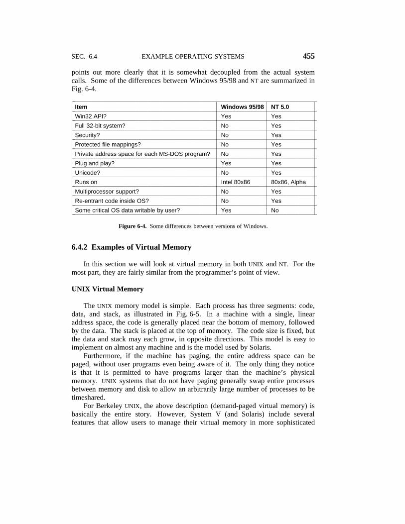
SEC. 6.4 EXAMPLE OPERATING SYSTEMS 455
points out more clearly that it is somewhat decoupled from the actual systemcalls. Some of the differences between Windows 95/98 and NT are summarized inFig. 6-4.2222222222222222222222222222222222222222222222222222222222222222222222222222222222Item Windows 95/98 NT 5.02222222222222222222222222222222222222222222222222222222222222222222222222222222222Win32 API? Yes Yes2222222222222222222222222222222222222222222222222222222222222222222222222222222222Full 32-bit system? No Yes2222222222222222222222222222222222222222222222222222222222222222222222222222222222Security? No Yes2222222222222222222222222222222222222222222222222222222222222222222222222222222222Protected file mappings? No Yes2222222222222222222222222222222222222222222222222222222222222222222222222222222222Private address space for each MS-DOS program? No Yes2222222222222222222222222222222222222222222222222222222222222222222222222222222222Plug and play? Yes Yes2222222222222222222222222222222222222222222222222222222222222222222222222222222222Unicode? No Yes2222222222222222222222222222222222222222222222222222222222222222222222222222222222Runs on Intel 80x86 80x86, Alpha2222222222222222222222222222222222222222222222222222222222222222222222222222222222Multiprocessor support? No Yes2222222222222222222222222222222222222222222222222222222222222222222222222222222222Re-entrant code inside OS? No Yes2222222222222222222222222222222222222222222222222222222222222222222222222222222222Some critical OS data writable by user? Yes No22222222222222222222222222222222222222222222222222222222222222222222222222222222221111111111111111111
1111111111111111111
1111111111111111111
1111111111111111111
Figure 6-4. Some differences between versions of Windows.
6.4.2 Examples of Virtual Memory
In this section we will look at virtual memory in both UNIX and NT. For themost part, they are fairly similar from the programmer’s point of view.
UNIX Virtual Memory
The UNIX memory model is simple. Each process has three segments: code,data, and stack, as illustrated in Fig. 6-5. In a machine with a single, linearaddress space, the code is generally placed near the bottom of memory, followedby the data. The stack is placed at the top of memory. The code size is fixed, butthe data and stack may each grow, in opposite directions. This model is easy toimplement on almost any machine and is the model used by Solaris.
Furthermore, if the machine has paging, the entire address space can bepaged, without user programs even being aware of it. The only thing they noticeis that it is permitted to have programs larger than the machine’s physicalmemory. UNIX systems that do not have paging generally swap entire processesbetween memory and disk to allow an arbitrarily large number of processes to betimeshared.
For Berkeley UNIX, the above description (demand-paged virtual memory) isbasically the entire story. However, System V (and Solaris) include severalfeatures that allow users to manage their virtual memory in more sophisticated

456 THE OPERATING SYSTEM MACHINE LEVEL CHAP. 6
Address
0xFFFFFFFF
0Code
Data
Stack
Figure 6-5. The address space of a single UNIX process.
ways. Most important of these is the ability of a process to map a (portion of) afile onto part of its address space. For example, if a 12-KB file is mapped at vir-tual address 144K, a read to the word at address 144K reads the first word of thefile. In this way file I/O can be done without making system calls. Since somefiles may exceed the size of the virtual address space, it is also possible to map inonly a portion of a file instead of the whole file. The mapping is done first open-ing the file and getting back a file descriptor, fd, which is used to identify the fileto be mapped. Then the process makes a call
paddr = mmap(virtual3address, length, protection, flags, fd, file3offset)
which maps length bytes starting at file3offset in the file onto the virtual addressspace starting at virtual3address. Alternatively, the flags parameter can be set toask the system to choose a virtual address, which it then returns as paddr. Themapped region must be an integral number of pages and aligned at a page boun-dary. The protection parameter can specify any combination of read, write, orexecute permission. The mapping can be removed later with unmap.
Multiple processes can map onto the same file at the same time. Two optionsare provided for sharing. In the first one, all the pages are shared, so writes doneby one process are visible to all the others. This option provides a high-bandwidthcommunication path between processes. The other option shares the pages aslong as no process modifies them. However, as soon as any process attempts towrite on a page, it gets a protection fault, which causes the operating system togive it a private copy of the page to write on. This scheme, known as copy onwrite, is used when each of multiple processes needs the illusion it is the only onemapped onto a file.
Windows NT Virtual Memory
In NT, every user process has its own virtual address space. Virtual addressesare 32 bits long, so each process has 4 GB of virtual address space. The lower 2GB are available for the process’ code and data; the upper 2 GB allow (limited)access to kernel memory, except in Enterprise versions of NT in which the split

SEC. 6.4 EXAMPLE OPERATING SYSTEMS 457
can be 3 GB for the user and 1 GB for the kernel. The virtual address space isdemand paged, with a fixed page size (4 KB on the Pentium II).
Each virtual page can be in one of three states: free, reserved, or committed.A free page is not currently [Hin use and a reference to it causes a page fault.When a process is started, all of its pages are in free state until the program andinitial data are mapped into its address space. Once code or data is mapped onto apage, the page is said to be committed. A reference to a committed page ismapped using the virtual memory hardware and succeeds if the page is in mainmemory. If the page is not in main memory, a page fault occurs and the operatingsystem finds and brings in the page from disk. A virtual page can also be inreserved state, meaning it is not available for being mapped until the reservationis explicitly removed. In addition to the free, reserved, and committed attributes,pages also have other attributes, such as being readable, writable, and executable.The top 64 KB and bottom 64 KB of memory are always free, to catch pointererrors (uninitialized pointers are often 0 or −1).
Each committed page has a shadow page on the disk where it is kept when itis not in main memory. Free and reserved pages do not have shadow pages, soreferences to them cause page faults (the system cannot bring in a page from diskif there is no page on disk). The shadow pages on the disk are arranged into oneor more paging files. The operating system keeps track of which virtual pagemaps onto which part of which paging file. For (execute only) program text, theexecutable binary file contains the shadow pages; for data pages, special pagingfiles are used.
NT, like System V, allows files to be mapped directly onto regions of the vir-tual address spaces (i.e., runs of consecutive pages). Once a file has been mappedonto the address space, it can be read or written using ordinary memory refer-ences.
Memory-mapped files are implemented in the same way as other committedpages, only the shadow pages can be in the disk file instead of in the paging file.As a result, when a file is mapped in, the version in memory may not be identicalto the disk version (due to recent writes to the virtual address space). However,when the file is unmapped or is explicitly flushed, the disk version is brought upto date.
NT explicitly allows two or more processes to map in the same file at the sametime, possibly at different virtual addresses. By reading and writing memorywords, the processes can now communicate with each other and pass data backand forth at very high bandwidth, since no copying is required. Differentprocesses may have different access permissions. Since all the processes using amapped file share the same pages, changes made by one of them are immediatelyvisible to all the others, even if the disk file has not yet been updated.
The Win32 API contains a number of functions that allow a process tomanage its virtual memory explicitly. The most important of these functions arelisted in Fig. 6-6. All of them operate on a region consisting either of a single

458 THE OPERATING SYSTEM MACHINE LEVEL CHAP. 6
page or a sequence of two or more pages that are consecutive in the virtualaddress space.
2222222222222222222222222222222222222222222222222222222222222222222222222222222API function Meaning2222222222222222222222222222222222222222222222222222222222222222222222222222222
VirtualAlloc Reserve or commit a region2222222222222222222222222222222222222222222222222222222222222222222222222222222VirtualFree Release or decommit a region2222222222222222222222222222222222222222222222222222222222222222222222222222222VirtualProtect Change the read/write/execute protection on a region2222222222222222222222222222222222222222222222222222222222222222222222222222222VirtualQuery Inquire about the status of a region2222222222222222222222222222222222222222222222222222222222222222222222222222222VirtualLock Make a region memory resident (i.e., disable paging for it)2222222222222222222222222222222222222222222222222222222222222222222222222222222VirtualUnlock Make a region pageable in the usual way2222222222222222222222222222222222222222222222222222222222222222222222222222222CreateFileMapping Create a file mapping object and (optionally) assign it a name2222222222222222222222222222222222222222222222222222222222222222222222222222222MapViewOfFile Map (part of) a file into the address space2222222222222222222222222222222222222222222222222222222222222222222222222222222UnmapViewOfFile Remove a mapped file from the address space2222222222222222222222222222222222222222222222222222222222222222222222222222222OpenFileMapping Open a previously created file mapping object222222222222222222222222222222222222222222222222222222222222222222222222222222211
1111111111111111
111111111111111111
111111111111111111
Figure 6-6. The principal API functions for managing virtual memory in Win-dows NT.
The first four API functions are self-explanatory. The next two give a processthe ability to hardwire up to 30 pages in memory so they will not be paged out andto undo this property. A real-time program might need this ability, for example.A limit is enforced by the operating system to prevent processes from getting toogreedy. Although not shown in Fig. 6-6, NT also has API functions to allow a pro-cess to access the virtual memory of a different process over which it has beengiven control (i.e., for which it has a handle).
The last four API functions listed are for managing memory-mapped files. Tomap a file, a file mapping object must first be created, with CreateFileMapping.This function returns a handle to the file mapping object and optionally enters aname for it into the file system so another process can use it. The next two func-tions map and unmap files, respectively. The last one can be used by a process tomap in a file currently also mapped in by a different process. In this way, two ormore processes can share regions of their address spaces.
These API functions are the basic ones upon which the rest of the memorymanagement system is built. For example, there are API functions for allocatingand freeing data structures on one or more heaps. Heaps are used for storing datastructures that are dynamically created and destroyed. The heaps are not garbagecollected, so it is up to user software to free blocks of virtual memory that are nolonger in use. (Garbage collection is the automatic removal of unused data struc-tures by the system.) Heap usage in NT is similar to the use of the malloc functionin UNIX systems, except that there can be multiple independently managed heaps.

SEC. 6.4 EXAMPLE OPERATING SYSTEMS 459
6.4.3 Examples of Virtual I/O
The heart of any operating system is providing services to user programs,mostly I/O services such as reading and writing files. Both UNIX and NT offer awide variety of I/O services to user programs. For most UNIX system calls, NT hasan equivalent call, but the reverse is not true as NT has far more calls and each ofthem is far more complicated than its UNIX counterpart.
UNIX Virtual I/O
Much of the popularity of the UNIX system can be traced directly to its simpli-city, which, in turn, is a direct result of the organization of the file system. Anordinary file is a linear sequence of 8-bit bytes starting at 0 and going up to amaximum of 232 − 1 bytes. The operating system itself imposes no record struc-ture on files, although many user programs regard ASCII text files as sequences oflines, each line terminated by a line feed.
Associated with every open file is a pointer to the next byte to be read or writ-ten. The read and write system calls read and write data starting at the file posi-tion indicated by the pointer. Both calls advance the pointer after the operation byan amount equal to the number of bytes transferred. However, random access tofiles is possible by explicitly setting the file pointer to a specific value.
In addition to ordinary files, the UNIX system also supports special files,which are used to access I/O devices. Each I/O device typically has one or morespecial files assigned to it. By reading and writing from the associated specialfile, a program can read or write from the I/O device. Disks, printers, terminals,and many other devices are handled this way.
The major UNIX file system calls are listed in Fig. 6-7. The creat call (withoutthe e) can be used to create a new file. It is not strictly necessary any more,because open can also create a new file now. Unlink removes a file, assuming thatthe file is in only one directory.
Open is used to open existing files (and create new ones). The mode flag tellshow to open it (for reading, for writing, etc.). The call returns a small integercalled a file descriptor that identifies the file in subsequent calls. The actual fileI/O is done with read and write, each of which has a file descriptor indicatingwhich file to use, a buffer for the data to go to or come from, and a byte count tel-ling how much data to transmit. Lseek is used to position the file pointer, makingrandom access to files possible.
Stat returns information about a file, including its size, time of last access,owner, and more. Chmod changes the protection mode of a file, for example,allowing or forbidding users other than the owner from reading it. Finally, fcntldoes various miscellaneous operations on a file, such as locking or unlocking it.
Figure 6-8 illustrates how the major file I/O calls work. This code is minimaland does not include the necessary error checking. Before entering the loop, the

460 THE OPERATING SYSTEM MACHINE LEVEL CHAP. 6
222222222222222222222222222222222222222222222222222222222222222222222222222222System call Meaning222222222222222222222222222222222222222222222222222222222222222222222222222222
creat(name, mode) Create a file; mode specifies the protection mode222222222222222222222222222222222222222222222222222222222222222222222222222222unlink(name) Delete a file (assuming that there is only 1 link to it)222222222222222222222222222222222222222222222222222222222222222222222222222222open(name, mode) Open or create a file and return a file descriptor222222222222222222222222222222222222222222222222222222222222222222222222222222close(fd) Close a file222222222222222222222222222222222222222222222222222222222222222222222222222222read(fd, buffer, count) Read count bytes into buffer222222222222222222222222222222222222222222222222222222222222222222222222222222write(fd, buffer, count) Write count bytes from buffer222222222222222222222222222222222222222222222222222222222222222222222222222222lseek(fd, offset, w) Move the file pointer as required by offset and w222222222222222222222222222222222222222222222222222222222222222222222222222222stat(name, buffer) Return information about a file222222222222222222222222222222222222222222222222222222222222222222222222222222chmod(name, mode) Change the protection mode of a file222222222222222222222222222222222222222222222222222222222222222222222222222222fcntl(fd, cmd, ...) Do various control operations such as locking (part of) a file222222222222222222222222222222222222222222222222222222222222222222222222222222111111111111111111
111111111111111111
111111111111111111
Figure 6-7. The principal UNIX file system calls.
program opens an existing file, data, and creates a new file, newf. Each callreturns a file descriptor, infd, and outfd, respectively. The second parameters tothe two calls are protection bits that specify that the files are to be read and writ-ten, respectively. Both calls return a file descriptor. If either open or creat fails, anegative file descriptor is returned, telling that the call failed.
// Open the file descriptorsinfd = open(′′data′′, 0);outfd = creat(′′newf′′, ProtectionBits);
// Copy loopdo {
count = read(infd, buffer, bytes);if (count > 0) write(outfd, buffer, count);
} while (count > 0);
// Close the filesclose(infd);close(outfd);
Figure 6-8. A program fragment for copying a file using the UNIX system calls.This fragment is in C because Java hides the low-level system calls and we aretrying to expose them.
The call to read has three parameters: a file descriptor, a buffer, and a bytecount. The call tries to read the desired number of bytes from the indicated fileinto the buffer. The number of bytes actually read is returned in count, which willbe smaller than bytes if the file was too short. The write call deposits the newlyread bytes on the output file. The loop continues until the input file has beencompletely read, at which time the loop terminates and both files are closed.

SEC. 6.4 EXAMPLE OPERATING SYSTEMS 461
File descriptors in UNIX are small integers (usually below 20). File descrip-tors 0, 1, and 2 are special and correspond to standard input, standard output,and standard error, respectively. Normally, these refer to the keyboard, thedisplay, and the display, respectively, but they can be redirected to files by theuser. Many UNIX programs get their input from standard input and write the pro-cessed output on standard output. Such programs are often called filters.
Closely related to the file system is the directory system. Each user may havemultiple directories, with each directory containing both files and subdirectories.UNIX systems normally are configured with a main directory, called the rootdirectory, containing subdirectories bin (for frequently executed programs), dev(for the special I/O device files), lib (for libraries), and usr (for user directories),as shown in Fig. 6-9. In this example, the usr directory contains subdirectories forast and jim. The ast directory contains two files, data and foo.p, and a subdirec-tory, bin, containing four games.
Files can be named by giving their path from the root directory. A path con-tains a list of all the directories traversed from the root to the file, with directorynames separated by slashes. For example, the absolute path name of game2 is/usr/ast/bin/game2. A path starting at the root is called an absolute path.
At every instant, each running program has a working directory. Path namesmay also be relative to the working directory, in which case they do not beginwith a slash, to distinguish them from absolute path names. Such paths are calledrelative paths. When /usr/ast is the working directory, game3 can be accessedusing the path bin/game3. A user may create a link to someone else’s file usingthe link system call. In the above example, /usr/ast/bin/game3 and /usr/jim/jottoboth access the same file. To prevent cycles in the directory system, links are notpermitted to directories. The calls and creat take either absolute or relative pathnames as arguments.
The major directory management system calls in UNIX are listed in Fig. 6-10.Mkdir creates a new directory and rmdir deletes an existing (empty) directory. Thenext three calls are used to read directory entries. The first one opens the direc-tory, the next one reads entries from it, and the last one closes the directory. Chdirchanges the working directory.
Link makes a new directory entry with the new entry pointing to an existingfile. For example, the entry /usr/jim/jotto might have been created by the call
link(′′/usr/ast/bin/game3′′, ′′/usr/jim/jotto′′)
or an equivalent call using relative path names, depending on the working direc-tory of the program making the call. Unlink removes a directory entry. If the filehas only one link, the file is deleted. If it has two or more links, it is kept. It doesnot matter whether a removed link is the original or a copy made later. Once alink is made, it is a first-class citizen, indistinguishable from the original. The call
unlink(′′/usr/ast/bin/game3′′)
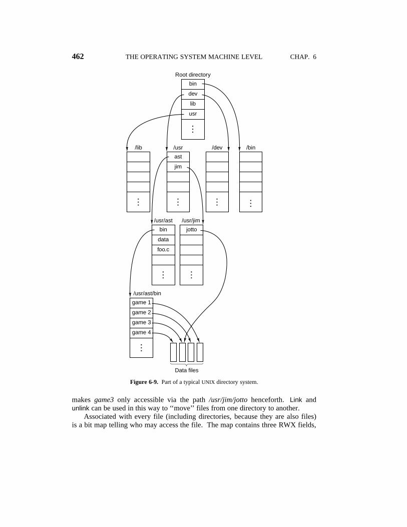
462 THE OPERATING SYSTEM MACHINE LEVEL CHAP. 6
/usr/ast/bin
Data files
game 1
game 2
game 3
game 4
…
/usr/ast
bin
data
foo.c…
/usr/jim
jotto
…
Root directory
bin
dev
lib
usr
…
/lib
…
/usr
ast
jim
…
/dev
…
/bin…
Figure 6-9. Part of a typical UNIX directory system.
makes game3 only accessible via the path /usr/jim/jotto henceforth. Link andunlink can be used in this way to ‘‘move’’ files from one directory to another.
Associated with every file (including directories, because they are also files)is a bit map telling who may access the file. The map contains three RWX fields,

SEC. 6.4 EXAMPLE OPERATING SYSTEMS 463
2222222222222222222222222222222222222222222222222222222222222222222222222System call Meaning2222222222222222222222222222222222222222222222222222222222222222222222222
mkdir(name, mode) Create a new directory2222222222222222222222222222222222222222222222222222222222222222222222222rmdir(name) Delete an empty directory2222222222222222222222222222222222222222222222222222222222222222222222222opendir(name) Open a directory for reading2222222222222222222222222222222222222222222222222222222222222222222222222readdir(dirpointer) Read the next entry in a directory2222222222222222222222222222222222222222222222222222222222222222222222222closedir(dirpointer) Close a directory2222222222222222222222222222222222222222222222222222222222222222222222222chdir(dirname) Change working directory to dirname2222222222222222222222222222222222222222222222222222222222222222222222222link(name1, name2) Create a directory entry name2 pointing to name12222222222222222222222222222222222222222222222222222222222222222222222222unlink(name) Remove name from its directory2222222222222222222222222222222222222222222222222222222222222222222222222111111111111111
111111111111111
111111111111111
Figure 6-10. The principal UNIX directory management calls.
the first controlling the Read, Write, eXecute permissions for the owner, thesecond for others in the owner’s group, and the third for everybody else. ThusRWX R-X --X means that the owner can read the file, write the file, and executethe file (obviously, it is an executable program, or execute would be off), whereasothers in his group can read or execute it and strangers can only execute it. Withthese permissions, strangers can use the program but not steal (copy) it becausethey do not have read permission. The assignment of users to groups is done bythe system administrator, usually called the superuser. The superuser also hasthe power to override the protection mechanism and read, write, or execute anyfile.
Let us now briefly examine how files and directories are implemented inUNIX. For a more complete treatment, see (Vahalia, 1996). Associated with eachfile (and each directory, because a directory is also a file) is a 64-byte block ofinformation called an i-node. The i-node tells who owns the file, what the per-missions are, where to find the data, and similar things. The i-nodes for the fileson each disk are located either in numerical sequence at the beginning of the disk,or if the disk is split up into groups of cylinders, at the start of a cylinder group.Thus given an i-node number, the UNIX system can locate the i-node by simplycalculating its disk address.
A directory entry consists of two parts: a file name and an i-node number.When a program executes
open(′′foo.c′′, 0)
the system searches the working directory for the file name, ‘‘foo.c,’’ in order tolocate the i-node number for that file. Having found the i-node number, it canthen read in the i-node, which tells it all about the file.
When a longer path name is specified, the basic steps outlined above are re-peated several times until the full path has been parsed. For example, to locatethe i-node number for /usr/ast/data, the system first searches the root directory for
464 THE OPERATING SYSTEM MACHINE LEVEL CHAP. 6
an entry usr. Having found the i-node for usr, it can read that file (a directory is afile in UNIX). In this file it looks for an entry ast, thus locating the i-node numberfor the file /usr/ast. By reading /usr/ast, the system can then find the entry fordata, and thus the i-node number for /usr/ast/data. Given the i-node number forthe file, it can then find out everything about the file from the i-node.
The format, contents, and layout of an i-node vary somewhat from system tosystem (especially when networking is in use), but the following items are typi-cally found in each i-node.
1. The file type, the 9 RWX protection bits, and a few other bits.
2. The number of links to the file (number of directory entries for it).
3. The owner’s identity.
4. The owner’s group.
5. The file length in bytes.
6. Thirteen disk addresses.
7. The time the file was last read.
8. The time the file was last written.
9. The time the i-node was last changed.
The file type distinguishes ordinary files, directories, and two kinds of specialfiles, for block-structured and unstructured I/O devices, respectively. The numberof links and the owner identification have already been discussed. The file lengthis a 32-bit integer giving the highest byte that has a value. It is perfectly legal tocreate a file, do an lseek to position 1,000,000, and write 1 byte, which yields afile of length 1,000,001. The file would not, however, require storage for all the‘‘missing’’ bytes.
The first 10 disk addresses point to data blocks. With a block size of 1024bytes, files up to 10,240 bytes can be handled this way. Address 11 points to adisk block, called an indirect block, which contains 256 disk addresses. Files upto 10,240 + 256 × 1024 = 272,384 bytes are handled this way. For still largerfiles, address 12 points to a block containing the addresses of 256 indirect blocks,which takes care of files up to 272,384 + 256 × 256 × 1024 = 67,381,248 bytes. Ifthis double indirect block scheme is still too small, disk address 13 is used topoint to a triple indirect block containing the addresses of 256 double indirectblocks. Using the direct, single, double, and triple indirect addresses, up to16,843,018 blocks can be addressed giving a theoretical maximum file size of17,247,250,432 bytes. Since file pointers are limited to 32 bits, the practicalupper limit is actually 4,294,967,295 bytes. Free disk blocks are kept on a linkedlist. When a new block is needed, the next block is plucked from the list. As aresult, the blocks of each file are scattered randomly around the disk.

SEC. 6.4 EXAMPLE OPERATING SYSTEMS 465
To make disk I/O more efficient, when a file is opened, its i-node is copied toa table in main memory and is kept there for handy reference as long as the fileremains open. In addition, a pool of recently referenced disk blocks is maintainedin memory. Because most files are read sequentially, it often happens that a filereference requires the same disk block as the previous reference. To strengthenthis effect, the system also tries to read the next block in a file, before it is refer-enced, in order to speed up processing. All this optimization is hidden from theuser; when a user issues a read call, the program is suspended until the requesteddata are available in the buffer.
With this background information, we can now see how file I/O works. Opencauses the system to search the directories for the specified path. If the search issuccessful, the i-node is read into an internal table. Reads and writes require thesystem to compute the block number from the current file position. The diskaddresses of the first 10 blocks are always in main memory (in the i-node);higher-numbered blocks require one or more indirect blocks to be read first.Lseek just changes the current position pointer without doing any I/O.
Link and unlink are also simple to understand now. Link looks up its first argu-ment to find the i-node number. Then it creates a directory entry for the secondargument, putting the i-node number of the first file in that entry. Finally, itincreases the link count in the i-node by one. Unlink removes a directory entryand decrements the link count in the i-node. If it is zero, the file is removed andall the blocks are put back on the free list.
Windows NT Virtual I/O
NT supports several file systems, the most important of which are NTFS (NTFile System) and the FAT (File Allocation Table) file system. The former is anew file system developed specifically for NT; the latter is the old MS-DOS file sys-tem, which is also used on Windows 95/98 (albeit with support for longer filenames). Since the FAT file system is basically obsolete (although several hun-dred million people are still using it), we will study NTFS below. Starting withNT 5.0, the FAT32 file system used in later versions of Windows 95 and in Win-dows 98 was also supported.
File names in NTFS can be up to 255 characters long. File names are inUnicode, allowing people in countries not using the Latin alphabet (e.g., Japan,India, and Israel) to write file names in their native language. (In fact, NT usesUnicode throughout internally; versions starting with NT 5.0 have a single binarythat can be used in any country and still use the local language because all themenus, error messages, etc., are kept in country-dependent configuration files.)NTFS fully supports case-sensitive names (so foo is different from FOO). Unfor-tunately, the Win32 API does not fully support case-sensitivity for file names andnot at all for directory names, so this advantage is lost to programs using Win32.

466 THE OPERATING SYSTEM MACHINE LEVEL CHAP. 6
As with UNIX, a file is just a linear sequence of bytes, although up to a max-imum of 264 − 1. File pointers also exist, as in UNIX, but are 64 bits wide ratherthan 32 bits, to handle the maximum length file. The Win32 API function callsfor file and directory manipulation are roughly similar to their UNIX counterparts,except most have more parameters and the security model is different. Opening afile returns a handle, which is then used for reading and writing the file. How-ever, unlike in UNIX, handles are not small integers, and standard input, standardoutput, and standard error have to be acquired explicitly rather than being prede-fined as 0, 1, and 2 (except in console mode, where they are preopened). Theprincipal Win32 API functions for file management are listed in Fig. 6-11.
2222222222222222222222222222222222222222222222222222222222222222222222222222222API function UNIX Meaning2222222222222222222222222222222222222222222222222222222222222222222222222222222
CreateFile open Create a file or open an existing file; return a handle2222222222222222222222222222222222222222222222222222222222222222222222222222222DeleteFile unlink Destroy an existing file2222222222222222222222222222222222222222222222222222222222222222222222222222222CloseHandle close Close a file2222222222222222222222222222222222222222222222222222222222222222222222222222222ReadFile read Read data from a file2222222222222222222222222222222222222222222222222222222222222222222222222222222WriteFile write Write data to a file2222222222222222222222222222222222222222222222222222222222222222222222222222222SetFilePointer lseek Set the file pointer to a specific place in the file2222222222222222222222222222222222222222222222222222222222222222222222222222222GetFileAttributes stat Return the file properties2222222222222222222222222222222222222222222222222222222222222222222222222222222LockFile fcntl Lock a region of the file to provide mutual exclusion2222222222222222222222222222222222222222222222222222222222222222222222222222222UnlockFile fcntl Unlock a previously locked region of the file22222222222222222222222222222222222222222222222222222222222222222222222222222221
111111111111111
1111111111111111
1111111111111111
1111111111111111
Figure 6-11. The principal Win32 API functions for file I/O. The secondcolumn gives the nearest UNIX equivalent.
Let us now examine these calls briefly. CreateFile can be used to create anew file and return a handle to it. This API function is also used to open existingfiles as there is no open API function. We have not listed the parameters for theNT API functions because they are so voluminous. As an example, CreateFile hasseven parameters, as follows:
1. A pointer to the name of the file to create or open.
2. Flags telling whether the file can be read, written, or both.
3. Flags telling whether multiple processes can open the file at once.
4. A pointer to the security descriptor, telling who can access the file.
5. Flags telling what to do if the file exists/does not exist.
6. Flags dealing with attributes such as archiving, compression, etc.
7. The handle of a file whose attributes should be cloned for the new file.

SEC. 6.4 EXAMPLE OPERATING SYSTEMS 467
The next six API functions in Fig. 6-11 are fairly similar to the correspondingUNIX system calls. The last two allow a region of a file to be locked and unlockedto permit a process to get guaranteed mutual exclusion to it.
Using these API functions, it is possible to write a procedure to copy a file,analogous to the UNIX version of Figure 6-1. Such a procedure (without any errorchecking) is shown in Fig. 6-12. It has been designed to mimic the structure ofFigure 6-8. In practice, one would not have to program a copy file program sinceCopyFile is an API function (which executes something close to this program as alibrary procedure).
// Open files for input and output.inhandle = CreateFile(′′data′′, GENERIC3READ, 0, NULL, OPEN3EXISTING, 0, NULL);outhandle = CreateFile( ′′newf′′, GENERIC3WRITE, 0, NULL, CREATE3ALWAYS,
FILE3ATTRIBUTE3NORMAL, NULL);
// Copy the file.do {
s = ReadFile(inhandle, buffer, BUF3SIZE, &count, NULL);if (s > 0 && count > 0) WriteFile(outhandle, buffer, count, &ocnt, NULL);
while (s > 0 && count > 0);
// Close the files.CloseHandle(inhandle);CloseHandle(outhandle);
Figure 6-12. A program fragment for copying a file using the Windows NTAPI functions. This fragment is in C because Java hides the low-level systemcalls and we are trying to expose them.
NT supports a hierarchical file system, similar to the UNIX file system. Theseparator between component names is \ however, instead of /, a fossil inheritedfrom MS-DOS. There is a concept of a current working directory and path namescan be relative or absolute. One significant difference with UNIX, however, isUNIX allows the file systems on different disks and machines to be mountedtogether in a single naming tree, thus hiding the disk structure from all software.NT 4.0 does not have this property, so absolute file names must begin with a driveletter indicating which logical disk is meant, as in C:\windows\system\foo.dll.Starting with NT 5.0, UNIX-style 5.0 mounting of file systems was added.
The major directory management API functions are given in Fig. 6-13, againalong with their nearest UNIX equivalents. The functions are hopefully self-explanatory.
Note that NT 4.0 did not support file links. At the level of the graphical desk-top, shortcuts were supported, but these constructions were internal to the desktopand had no counterpart in the file system itself. An application program could notenter a file in a second directory without copying the entire file. Starting with NT
5.0 file linking was added to the file system proper.
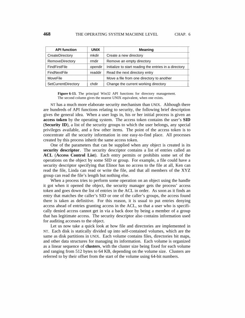
468 THE OPERATING SYSTEM MACHINE LEVEL CHAP. 6
2222222222222222222222222222222222222222222222222222222222222222222222222222222API function UNIX Meaning2222222222222222222222222222222222222222222222222222222222222222222222222222222
CreateDirectory mkdir Create a new directory2222222222222222222222222222222222222222222222222222222222222222222222222222222RemoveDirectory rmdir Remove an empty directory2222222222222222222222222222222222222222222222222222222222222222222222222222222FindFirstFile opendir Initialize to start reading the entries in a directory2222222222222222222222222222222222222222222222222222222222222222222222222222222FindNextFile readdir Read the next directory entry2222222222222222222222222222222222222222222222222222222222222222222222222222222MoveFile Move a file from one directory to another2222222222222222222222222222222222222222222222222222222222222222222222222222222SetCurrentDirectory chdir Change the current working directory222222222222222222222222222222222222222222222222222222222222222222222222222222211
1111111111
111111111111
111111111111
111111111111
Figure 6-13. The principal Win32 API functions for directory management.The second column gives the nearest UNIX equivalent, when one exists.
NT has a much more elaborate security mechanism than UNIX. Although thereare hundreds of API functions relating to security, the following brief descriptiongives the general idea. When a user logs in, his or her initial process is given anaccess token by the operating system. The access token contains the user’s SID(Security ID), a list of the security groups to which the user belongs, any specialprivileges available, and a few other items. The point of the access token is toconcentrate all the security information in one easy-to-find place. All processescreated by this process inherit the same access token.
One of the parameters that can be supplied when any object is created is itssecurity descriptor. The security descriptor contains a list of entries called anACL (Access Control List). Each entry permits or prohibits some set of theoperations on the object by some SID or group. For example, a file could have asecurity descriptor specifying that Elinor has no access to the file at all, Ken canread the file, Linda can read or write the file, and that all members of the XYZgroup can read the file’s length but nothing else.
When a process tries to perform some operation on an object using the handleit got when it opened the object, the security manager gets the process’ accesstoken and goes down the list of entries in the ACL in order. As soon as it finds anentry that matches the caller’s SID or one of the caller’s groups, the access foundthere is taken as definitive. For this reason, it is usual to put entries denyingaccess ahead of entries granting access in the ACL, so that a user who is specifi-cally denied access cannot get in via a back door by being a member of a groupthat has legitimate access. The security descriptor also contains information usedfor auditing accesses to the object.
Let us now take a quick look at how file and directories are implemented inNT. Each disk is statically divided up into self-contained volumes, which are thesame as disk partitions in UNIX. Each volume contains files, directories bit maps,and other data structures for managing its information. Each volume is organizedas a linear sequence of clusters, with the cluster size being fixed for each volumeand ranging from 512 bytes to 64 KB, depending on the volume size. Clusters arereferred to by their offset from the start of the volume using 64-bit numbers.

SEC. 6.4 EXAMPLE OPERATING SYSTEMS 469
The main data structure in each volume is the MFT (Master File Table),which has an entry for each file and directory in the volume. These entries areanalogous to the i-nodes in UNIX. The MFT is itself a file, and as such can beplaced anywhere within the volume, thus eliminating the problem that UNIX haswith bad disk blocks in the middle of the i-nodes.
The MFT is shown in Fig. 6-14. It begins with a header containing informa-tion about the volume, such as (pointers to) the root directory, the boot file, thebad-block file, the free-list administration, etc. After that comes an entry per fileor directory, 1 KB except when the cluster size is 2 KB or more. Each entry con-tains all the metadata (administrative information) about the file or directory.Several formats are allowed, one of which is shown in Fig. 6-14.
MFTheader
MFT entry for one file
Standardinformation
MS-DOSnameFile name Security Data
Masterfile
table
Figure 6-14. The Windows NT master file table.
The standard information field contains information such as the time stampsneeded by POSIX, the hard link count, the read-only and archive bits, etc. It is afixed-length field and always present. The file name is variable length, up to 255Unicode characters. In order to make such files accessible to old 16-bit programs,files can also have a MS-DOS name, which consists of 8 alphanumeric charactersoptionally followed by a dot and an extension of up to 3 alphanumeric characters.If the actual file name conforms to the MS-DOS 8+3 naming rule, a secondary MS-
DOS name is not used.Next comes the security information. In versions up to and including NT 4.0,
the security field contained the actual security descriptor. Starting with NT 5.0, allthe security information was centralized in a single file, with the security fieldsimply pointing to the relevant part of this file.
For small files, the file data itself is actually contained in the MFT entry, sav-ing a disk access to fetch it. This idea is called an immediate file (Mullender andTanenbaum, 1987). For somewhat larger files, this field contains pointers to theclusters containing the data, or more commonly, runs of consecutive clusters so a
470 THE OPERATING SYSTEM MACHINE LEVEL CHAP. 6
single cluster number and a length can represent an arbitrary amount of file data.If a single MFT entry is insufficiently large to hold whatever information it is sup-posed to hold, one or more additional entries can be chained to it.
The maximum file size is 264 bytes. To get an idea of how big a 264-byte fileis, imagine that the file were written out in binary, with each 0 or 1 occupying 1mm of space. The 267-mm listing would be 15 light-years long, reaching farbeyond the solar system, to Alpha Centauri and back.
The NTFS file system has many other interesting properties including datacompression and fault tolerance using atomic transactions. Additional informa-tion about it can be found in (Solomon, 1998).
6.4.4 Examples of Process Management
Both UNIX and NT allow a job to be split up into multiple processes that canrun in (pseudo)parallel and communicate with each other, in the style of theproducer-consumer example discussed earlier. In this section we will discuss howprocesses are managed in both systems. Both systems also support parallelismwithin a single process using threads, so that will also be discussed.
UNIX Process Management
At any time, a UNIX process can create a subprocess that is an exact replica ofitself by executing the fork system call. The original process is called the parentand the new one is called the child. Right after the fork, the two processes areidentical and even share the same file descriptors. Thereafter, each one goes itsown way and does whatever it wants to, independent of the other one.
In many cases, the child process juggles the file descriptors in certain waysand then executes the exec system call, which replaces its program and data withthe program and data found in an executable file specified as parameter to theexec call. For example, when a user types a command xyz at a terminal, the com-mand interpreter (shell) executes fork to create a child process. This child processthen executes exec to run the xyz program.
The two processes run in parallel (with or without exec), unless the parentwishes to wait for the child to terminate before continuing. If the parent wishes towait, it executes either the wait or waitpid system call, which causes it to besuspended until the child finishes by executing exit. After the child finishes, theparent continues.
Processes can execute fork as often as they want, giving rise to a tree ofprocesses. In Fig. 6-15, for example, process A has executed fork twice, creatingtwo children, B and C. Then B also executed fork twice, and C executed it once,giving the final tree of six processes.
Processes in UNIX can communicate with each other via a structure called apipe. A pipe is a kind of buffer into which one process can write a stream of data

SEC. 6.4 EXAMPLE OPERATING SYSTEMS 471
Original process
Children of A
Grandchildren of AA A A
A
A A
Figure 6-15. A process tree in UNIX.
and another can take it out. Bytes are always retrieved from a pipe in the orderthey were written. Random access is not possible. Pipes do not preserve messageboundaries, so if one process does four 128-byte writes and the other does a 512-byte read, the reader will get all the data at once, with no indication that they werewritten in multiple operations.
In System V and Solaris, another way for processes to communicate is byusing message queues. A process can create a new message queue or open anexisting one using msgget. Using a message queue, a process can send messagesusing msgsnd and receive them using msgrecv. Messages sent this way differfrom data stuffed into a pipe in several ways. First, message boundaries arepreserved, whereas a pipe is just a byte stream. Second, messages have priorities,so urgent ones can skip ahead of less important ones. Third, messages are typed,and a msgrecv can specify a particular type, if desired.
Another communication mechanism is the ability of two or more processes toshare a region of their respective address spaces. UNIX handles this sharedmemory by mapping the same pages into the virtual address space of all the shar-ing processes. As a result, a write by one process into the shared region isimmediately visible to the other processes. This mechanism provides a very highbandwidth communication path between processes. The system calls involved inshared memory go by names like shmat and shmop.
Another feature of System V and Solaris is the availability of semaphores.These work essentially as described in the producer-consumer example given inthe text.
Another facility provided by all POSIX-conformant UNIX systems is the abilityto have multiple threads of control within a single process. These threads of con-trol, usually just called threads, are like lightweight processes that share a com-mon address space and everything associated with that address space, such as filedescriptors, environment variables, and outstanding timers. However, each threadhas its own program counter, own registers, and own stack. When a thread blocks(i.e., has to stop temporarily until I/O completes or some other event happens),other threads in the same process are still able to run. Two threads in the sameprocess operating as a producer and consumer are similar, but not identical, to twosingle-thread processes that are sharing a memory segment containing a buffer.

472 THE OPERATING SYSTEM MACHINE LEVEL CHAP. 6
The differences have to do with the fact that in the latter case, each process has itsown file descriptors, etc., whereas in the former case all of these items are shared.We saw the use of Java threads in our producer-consumer example earlier. Oftenthe Java runtime system uses a operating system thread for each of its threads, butit does not have to do this.
As an example of where threads might be useful, consider a World Wide Webserver. Such a server might keep a cache of commonly-used Web pages in mainmemory. If a request is for a page in the cache, the Web page is returned immedi-ately. Otherwise, it is fetched from disk. Unfortunately, waiting for the disktakes a long time (typically 20 msec), during which the process is blocked andcannot serve new incoming requests, even those for Web pages in the cache.
The solution is to have multiple threads within the server process, all of whichshare the common Web page cache. When one thread blocks, other threads canhandle new requests. To prevent blocking without threads, one could have multi-ple server processes, but this would probably entail replicating the cache, thuswasting valuable memory.
The UNIX standard for threads is called pthreads, and is defined by POSIX
(P1003.1C) It contains calls for managing and synchronizing threads. It is notdefined whether threads are managed by the kernel or entirely in user space. Themost commonly-used thread calls are listed in Fig. 6-16.2222222222222222222222222222222222222222222222222222222222222222222222222222222
Thread call Meaning2222222222222222222222222222222222222222222222222222222222222222222222222222222pthread3create Create a new thread in the caller’s address space2222222222222222222222222222222222222222222222222222222222222222222222222222222pthread3exit Terminate the calling thread2222222222222222222222222222222222222222222222222222222222222222222222222222222pthread3join Wait for a thread to terminate2222222222222222222222222222222222222222222222222222222222222222222222222222222pthread3mutex3init Create a new mutex2222222222222222222222222222222222222222222222222222222222222222222222222222222pthread3mutex3destroy Destroy a mutex2222222222222222222222222222222222222222222222222222222222222222222222222222222pthread3mutex3lock Lock a mutex2222222222222222222222222222222222222222222222222222222222222222222222222222222pthread3mutex3unlock Unlock a mutex2222222222222222222222222222222222222222222222222222222222222222222222222222222pthread3cond3init Create a condition variable2222222222222222222222222222222222222222222222222222222222222222222222222222222pthread3cond3destroy Destroy a condition variable2222222222222222222222222222222222222222222222222222222222222222222222222222222pthread3cond3wait Wait on a condition variable2222222222222222222222222222222222222222222222222222222222222222222222222222222pthread3cond3signal Release one thread waiting on a condition variable22222222222222222222222222222222222222222222222222222222222222222222222222222221
111111111111111111
1111111111111111111
1111111111111111111
Figure 6-16. The principal POSIX thread calls.
Let us briefly examine the thread calls shown in Fig. 6-16. The first call,pthread3create, creates a new thread. After successful completion, one morethread is running in the caller’s address space than was before the call. A threadthat has done its job and wants to terminate calls pthread3exit. A thread can waitfor another thread to exit by calling pthread3join. If the thread waited for hasalready exited, the pthread3join finishes immediately. Otherwise it blocks.
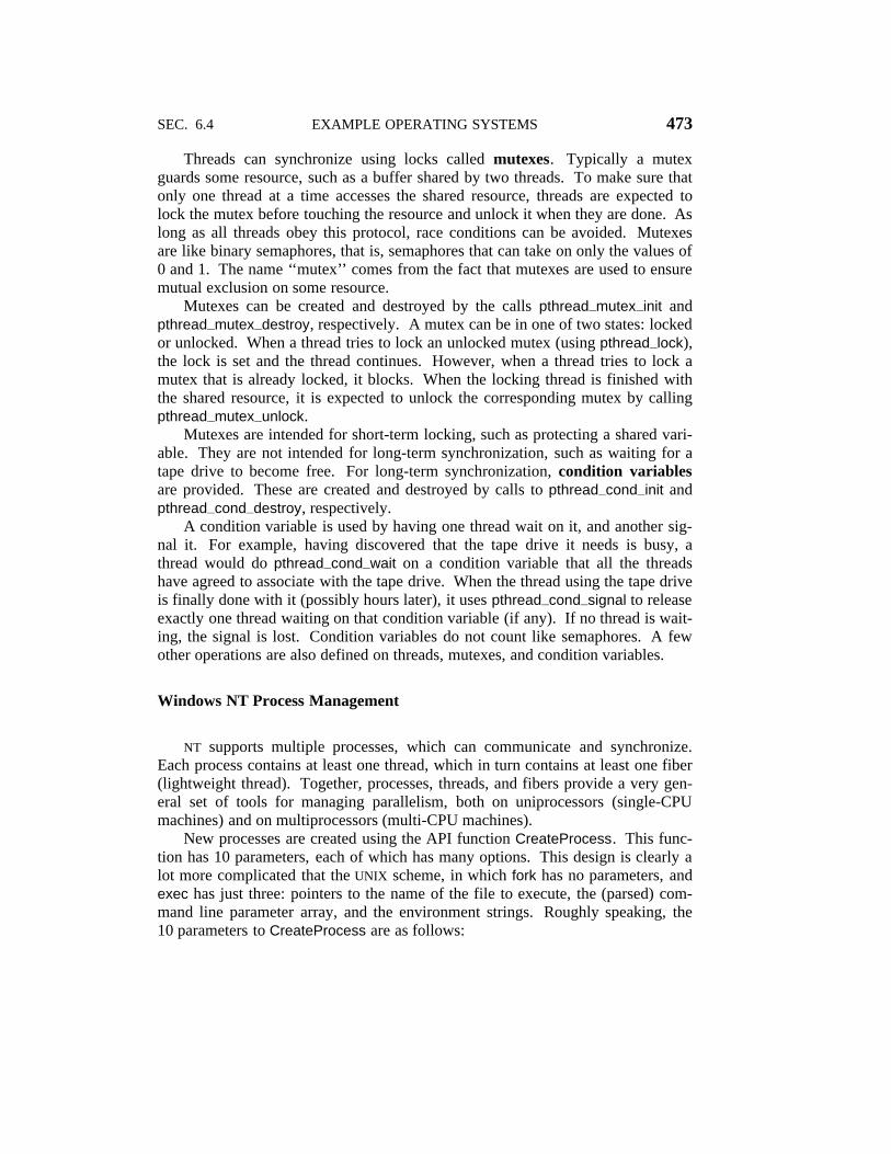
SEC. 6.4 EXAMPLE OPERATING SYSTEMS 473
Threads can synchronize using locks called mutexes. Typically a mutexguards some resource, such as a buffer shared by two threads. To make sure thatonly one thread at a time accesses the shared resource, threads are expected tolock the mutex before touching the resource and unlock it when they are done. Aslong as all threads obey this protocol, race conditions can be avoided. Mutexesare like binary semaphores, that is, semaphores that can take on only the values of0 and 1. The name ‘‘mutex’’ comes from the fact that mutexes are used to ensuremutual exclusion on some resource.
Mutexes can be created and destroyed by the calls pthread3mutex3init andpthread3mutex3destroy, respectively. A mutex can be in one of two states: lockedor unlocked. When a thread tries to lock an unlocked mutex (using pthread3lock),the lock is set and the thread continues. However, when a thread tries to lock amutex that is already locked, it blocks. When the locking thread is finished withthe shared resource, it is expected to unlock the corresponding mutex by callingpthread3mutex3unlock.
Mutexes are intended for short-term locking, such as protecting a shared vari-able. They are not intended for long-term synchronization, such as waiting for atape drive to become free. For long-term synchronization, condition variablesare provided. These are created and destroyed by calls to pthread3cond3init andpthread3cond3destroy, respectively.
A condition variable is used by having one thread wait on it, and another sig-nal it. For example, having discovered that the tape drive it needs is busy, athread would do pthread3cond3wait on a condition variable that all the threadshave agreed to associate with the tape drive. When the thread using the tape driveis finally done with it (possibly hours later), it uses pthread3cond3signal to releaseexactly one thread waiting on that condition variable (if any). If no thread is wait-ing, the signal is lost. Condition variables do not count like semaphores. A fewother operations are also defined on threads, mutexes, and condition variables.
Windows NT Process Management
NT supports multiple processes, which can communicate and synchronize.Each process contains at least one thread, which in turn contains at least one fiber(lightweight thread). Together, processes, threads, and fibers provide a very gen-eral set of tools for managing parallelism, both on uniprocessors (single-CPUmachines) and on multiprocessors (multi-CPU machines).
New processes are created using the API function CreateProcess. This func-tion has 10 parameters, each of which has many options. This design is clearly alot more complicated that the UNIX scheme, in which fork has no parameters, andexec has just three: pointers to the name of the file to execute, the (parsed) com-mand line parameter array, and the environment strings. Roughly speaking, the10 parameters to CreateProcess are as follows:

474 THE OPERATING SYSTEM MACHINE LEVEL CHAP. 6
1. A pointer to the name of the executable file.
2. The command line itself (unparsed).
3. A pointer to a security descriptor for the process.
4. A pointer to a security descriptor for the initial thread.
5. A bit telling whether the new process inherits the creator’s handles.
6. Miscellaneous flags (e.g., error mode, priority, debugging, consoles).
7. A pointer to the environment strings.
8. A pointer to the name of the new process’ current working directory.
9. A pointer to a structure describing the initial window on the screen.
10. A pointer to a structure that returns 18 values to the caller.
NT does not enforce any kind of parent-child or other hierarchy. All processesare created equal. However, since 1 of the 18 parameters returned to the creatingprocess is a handle to the new process (allowing considerable control over thenew process), there is an implicit hierarchy in terms of who has a handle to whom.Although these handles cannot just be passed directly to other processes, there is away for a process to make a handle suitable for another process and then give itthe handle, so the implicit process hierarchy may not last long.
Each process in NT is created with a single thread, but a process can createmore threads later on. Thread creation is simpler than process creation:CreateThread has only six parameters instead of 10: the security descriptor, thestack size, the starting address, a user-defined parameter, the initial state of thethread (ready or blocked), and the thread’s ID. The kernel does the thread crea-tion, so it is clearly aware of threads (i.e, they are not implemented purely in userspace as is the case in some other systems).
When the kernel does scheduling, it not only picks the process to run next butalso which thread in that process. This means that the kernel is always aware ofwhich threads are ready and which ones are blocked. Because threads are kernelobjects, they have security descriptors and handles. Since a handle for a threadcan be passed to another process, it is possible to have one process control thethreads in a different process. This feature is useful for debuggers, for example.
Threads in NT are relatively expensive because doing a thread switch requiresentering and later leaving the kernel. To provide very lightweight pseudoparallel-ism, NT provides fibers, which are like threads, but are scheduled in user space bythe program that created them (or its runtime system). Each thread can have mul-tiple fibers, the same way a process can have multiple threads, except that when afiber logically blocks, it puts itself on the queue of blocked fibers and selectsanother fiber to run in the context of its thread. The kernel is not aware of this

SEC. 6.4 EXAMPLE OPERATING SYSTEMS 475
transition because the thread keeps running, even though it may be first runningone fiber, then another. The kernel just manages processes and threads, not fibers.Fibers are useful, for example, when programs that manage their own threads areported to NT.
Processes can communicate in a wide variety of ways, including pipes, namedpipes, mailslots, sockets, remote procedure calls, and shared files. Pipes have twomodes: byte and message, selected at creation time. Byte-mode pipes work thesame way as in UNIX. Message-mode pipes are somewhat similar but preservemessage boundaries, so that four writes of 128 bytes will be read as four 128-bytemessages, and not as one 512-byte message, as would happen with byte-modepipes. Named pipes also exist and have the same two modes as regular pipes.Named pipes can also be used over a network; regular pipes cannot.
Mailslots are a feature of NT not present in UNIX. They are similar to pipes insome ways, but not all. For one thing, they are one-way, whereas pipes are two-way. They can also be used over a network but do not provide guaranteeddelivery. Finally, they allow the sending process to broadcast a message to manyreceivers, instead of to just one.
Sockets are like pipes, except that they normally connect processes on dif-ferent machines. However, they can also be used to connect processes on thesame machine. In general, there is usually little advantage to using a socket con-nection over a pipe or named pipe for intramachine communication.
Remote procedure calls are a way for process A to have process B call a pro-cedure in B’s address space on A’s behalf and return the result to A. Various res-trictions on the parameters exist. For example, it makes no sense to pass a pointerto a different process.
Finally, processes can share memory by mapping onto the same file at thesame time. All writes done by one process then appear in the address spaces ofthe other processes. Using this mechanism, the shared buffer used in ourproducer-consumer example can be easily implemented.
Just as NT provides numerous interprocess communication mechanisms, italso provides numerous synchronization mechanisms, including semaphores,mutexes, critical sections, and events. All of these mechanisms work on threads,not processes, so that when a thread blocks on a semaphore, other threads in thatprocess (if any) are not affected and can continue to run.
A semaphore is created using the CreateSemaphore API function, which caninitialize it to a given value and define a maximum value as well. Semaphores arekernel objects and thus have security descriptors and handles. The handle for asemaphore can be duplicated using DuplicateHandle and passed to another processso that multiple processes can synchronize on the same semaphore. Calls for upand down are present, although they have the somewhat peculiar names ofReleaseSemaphore (up) and WaitForSingleObject (down). It is also possible togive WaitForSingleObject a timeout, so the calling thread can be released eventu-ally, even if the semaphore remains at 0 (although timers reintroduce races).
476 THE OPERATING SYSTEM MACHINE LEVEL CHAP. 6
Mutexes are also kernel objects used for synchronization, but simpler thansemaphores because they do not have counters. They are essentially locks, withAPI functions for locking (WaitForSingleObject) and unlocking ReleaseMutex.Like semaphore handles, mutex handles can be duplicated and passed betweenprocesses so that threads in different processes can access the same mutex.
The third synchronization mechanism is based on critical sections, which aresimilar to mutexes, except local to the address space of the creating thread.Because critical sections are not kernel objects, they do not have handles or secu-rity descriptors and cannot be passed between processes. Locking and unlockingis done with EnterCriticalSection and LeaveCriticalSection, respectively. Becausethese API functions are performed entirely in user space, they are much fasterthan mutexes.
The last synchronization mechanism uses kernel objects called events. Athread can wait for an event to occur with WaitForSingleObject . A thread canrelease a single thread waiting on an event with SetEvent or it can release allthreads waiting on an event with PulseEvent. Events come in several flavors andhave a variety of options, too.
Events, mutexes, and semaphores can all be named and stored in the file sys-tem, like named pipes. Two or more processes can synchronize by opening thesame event, mutex, or semaphore, rather than having one of them create the objectand then make duplicate handles for the others, although the latter approach iscertainly an option as well.

7THE ASSEMBLY LANGUAGE LEVEL
1

2222222222222222222222222222222222222222222222222222222222222222222Programmer-years to
produce the program
Program execution
time in seconds2222222222222222222222222222222222222222222222222222222222222222222Assembly language 50 33High-level language 10 100
Mixed approach before tuningCritical 10% 1 90Other 90% 9 10
33 33Total 10 100
Mixed approach after tuningCritical 10% 6 30Other 90% 9 10
33 33Total 15 4022222222222222222222222222222222222222222222222222222222222222222221
111111111111111111
1111111111111111111
1111111111111111111
1111111111111111111
Figure 7-1. Comparison of assembly language and high-levellanguage programming, with and without tuning.

Label Opcode Operands Comments2222222222222222222222222222222222222222222222222222222222222222222222FORMULA: MOV EAX,I ; register EAX = I
ADD EAX,J ; register EAX = I + JMOV N,EAX ; N = I + J
I DW 3 ; reserve 4 bytes initialized to 3J DW 4 ; reserve 4 bytes initialized to 4N DW 0 ; reserve 4 bytes initialized to 0
(a)
Label Opcode Operands Comments2222222222222222222222222222222222222222222222222222222222222222222222FORMULA MOVE.L I, D0 ; register D0 = I
ADD.L J, D0 ; register D0 = I + JMOVE.L D0, N ; N = I + J
I DC.L 3 ; reserve 4 bytes initialized to 3J DC.L 4 ; reserve 4 bytes initialized to 4N DC.L 0 ; reserve 4 bytes initialized to 0
(b)
Label Opcode Operands Comments222222222222222222222222222222222222222222222222222222222222222222222222222222222222FORMULA: SETHI %HI(I),%R1 ! R1 = high-order bits of the address of I
LD [%R1+%LO(I)],%R1 ! R1 = ISETHI %HI(J),%R2 ! R2 = high-order bits of the address of JLD [%R2+%LO(J)],%R2 ! R2 = JNOP ! wait for J to arrive from memoryADD %R1,%R2,%R2 ! R2 = R1 + R2SETHI %HI(N),%R1 ! R1 = high-order bits of the address of NST %R2,[%R1+%LO(N)]
I: .WORD 3 ! reserve 4 bytes initialized to 3J: .WORD 4 ! reserve 4 bytes initialized to 4N: .WORD 0 ! reserve 4 bytes initialized to 0
(c)
Figure 7-2. Computation of N = I + J. (a) Pentium II. (b)Motorola 680x0. (c) SPARC.

222222222222222222222222222222222222222222222222222222222222222222222222222Pseudoinstr Meaning222222222222222222222222222222222222222222222222222222222222222222222222222SEGMENT Start a new segment (text, data, etc.) with certain attributes222222222222222222222222222222222222222222222222222222222222222222222222222ENDS End the current segment222222222222222222222222222222222222222222222222222222222222222222222222222ALIGN Control the alignment of the next instruction or data222222222222222222222222222222222222222222222222222222222222222222222222222EQU Define a new symbol equal to a given expression222222222222222222222222222222222222222222222222222222222222222222222222222DB Allocate storage for one or more (initialized) bytes222222222222222222222222222222222222222222222222222222222222222222222222222DD Allocate storage for one or more (initialized) 16-bit halfwords222222222222222222222222222222222222222222222222222222222222222222222222222DW Allocate storage for one or more (initialized) 32-bit words222222222222222222222222222222222222222222222222222222222222222222222222222DQ Allocate storage for one or more (initialized) 64-bit double words222222222222222222222222222222222222222222222222222222222222222222222222222PROC Start a procedure222222222222222222222222222222222222222222222222222222222222222222222222222ENDP End a procedure222222222222222222222222222222222222222222222222222222222222222222222222222MACRO Start a macro definition222222222222222222222222222222222222222222222222222222222222222222222222222ENDM End a macro definition222222222222222222222222222222222222222222222222222222222222222222222222222PUBLIC Export a name defined in this module222222222222222222222222222222222222222222222222222222222222222222222222222EXTERN Import a name from another module222222222222222222222222222222222222222222222222222222222222222222222222222INCLUDE Fetch and include another file222222222222222222222222222222222222222222222222222222222222222222222222222IF Start conditional assembly based on a given expression222222222222222222222222222222222222222222222222222222222222222222222222222ELSE Start conditional assembly if the IF condition above was false222222222222222222222222222222222222222222222222222222222222222222222222222ENDIF End conditional assembly222222222222222222222222222222222222222222222222222222222222222222222222222COMMENT Define a new start-of-comment character222222222222222222222222222222222222222222222222222222222222222222222222222PAGE Generate a page break in the listing222222222222222222222222222222222222222222222222222222222222222222222222222END Terminate the assembly program222222222222222222222222222222222222222222222222222222222222222222222222222111111111111111111111111111111111
111111111111111111111111111111111
111111111111111111111111111111111
Figure 7-3. Some of the pseudoinstructions available in thePentium II assembler (MASM).

MOV EAX,P SWAP MACROMOV EBX,Q MOV EAX,PMOV Q,EAX MOV EBX,QMOV P,EBX MOV Q,EAX
MOV P,EBXMOV EAX,P ENDMMOV EBX,QMOV Q,EAX SWAPMOV P,EBX
SWAP
(a) (b)
Figure 7-4. Assembly language code for interchanging P andQ twice. (a) Without a macro. (b) With a macro.

2222222222222222222222222222222222222222222222222222222222222222222222222222Item Macro call Procedure call2222222222222222222222222222222222222222222222222222222222222222222222222222
When is the call made? During assembly During execution2222222222222222222222222222222222222222222222222222222222222222222222222222Yes NoIs the body inserted into the object
program every place the call ismade?2222222222222222222222222222222222222222222222222222222222222222222222222222
No YesIs a procedure call instructioninserted into the object programand later executed?2222222222222222222222222222222222222222222222222222222222222222222222222222
No YesMust a return instruction be usedafter the call is done?2222222222222222222222222222222222222222222222222222222222222222222222222222
One per macro call 1How many copies of the body ap-pear in the object program?222222222222222222222222222222222222222222222222222222222222222222222222222211111111111111111
11111111111111111
11111111111111111
11111111111111111
Figure 7-5. Comparison of macro calls with procedure calls.

MOV EAX,P CHANGE MACRO P1, P2MOV EBX,Q MOV EAX,P1MOV Q,EAX MOV EBX,P2MOV P,EBX MOV P2,EAX
MOV P1,EBXMOV EAX,R ENDMMOV EBX,SMOV S,EAX CHANGE P, QMOV R,EBX
CHANGE R, S
(a) (b)
Figure 7-6. Nearly identical sequences of statements. (a)Without a macro. (b) With a macro.

Label Opcode Operands Comments Length ILC222222222222222222222222222222222222222222222222222222222222222222222222222MARIA: MOV EAX,I EAX = I 5 100
MOV EBX, J EBX = J 6 105ROBERTA: MOV ECX, K ECX = K 6 111
IMUL EAX, EAX EAX = I * I 2 117IMUL EBX, EBX EBX = J * J 3 119IMUL ECX, ECX ECX = K * K 3 122
MARILYN: ADD EAX, EBX EAX = I * I + J * J 2 125ADD EAX, ECX EAX = I * I + J * J + K * K 2 127
STEPHANY: JMP DONE branch to DONE 5 129
Figure 7-7. The instruction location counter (ILC) keeps trackof the address where the instructions will be loaded in memory.In this example, the statements prior to MARIA occupy 100bytes.
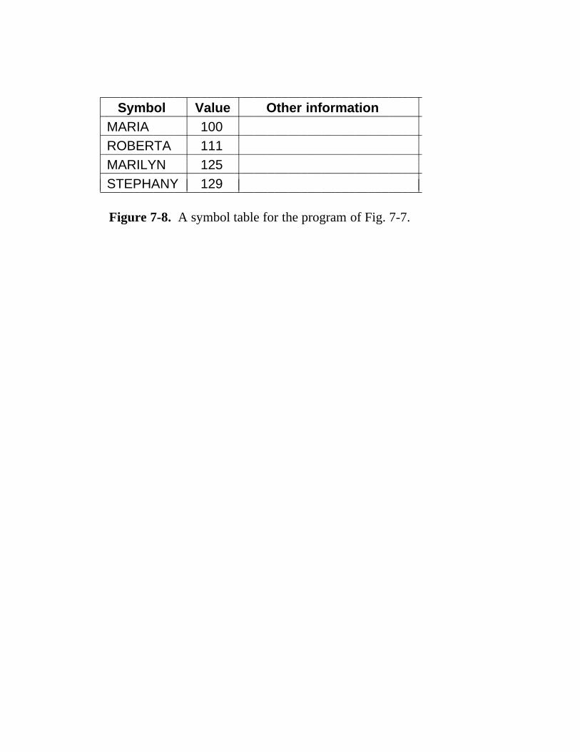
222222222222222222222222222222222222222222222222Symbol Value Other information222222222222222222222222222222222222222222222222
MARIA 100222222222222222222222222222222222222222222222222ROBERTA 111222222222222222222222222222222222222222222222222MARILYN 125222222222222222222222222222222222222222222222222STEPHANY 12922222222222222222222222222222222222222222222222211111111
11111111
11111111
11111111
Figure 7-8. A symbol table for the program of Fig. 7-7.

2222222222222222222222222222222222222222222222222222222222222222222222
OpcodeFirstoperand
Secondoperand
Hexadecimalopcode
Instruc-tion
length
Instruc-tion
class2222222222222222222222222222222222222222222222222222222222222222222222AAA — — 37 1 62222222222222222222222222222222222222222222222222222222222222222222222ADD EAX immed32 05 5 42222222222222222222222222222222222222222222222222222222222222222222222ADD reg reg 01 2 192222222222222222222222222222222222222222222222222222222222222222222222AND EAX immed32 25 5 42222222222222222222222222222222222222222222222222222222222222222222222AND reg reg 21 2 1922222222222222222222222222222222222222222222222222222222222222222222221
1111111111
11111111111
11111111111
11111111111
11111111111
11111111111
11111111111
Figure 7-9. A few excerpts from the opcode table for a Penti-um II assembler.

public static void pass3one( ) {// This procedure is an outline of pass one of a simple assembler.boolean more3input = true; // flag that stops pass oneString line, symbol, literal, opcode; // fields of the instructionint location3counter, length, value, type; // misc. variablesfinal int END3STATEMENT = −2; // signals end of input
location3counter = 0; // assemble first instruction at 0initialize3tables( ); // general initialization
while (more3input) { // more3input set to false by ENDline = read3next3line( ); // get a line of inputlength = 0; // # bytes in the instructiontype = 0; // which type (format) is the instruction
if (line3is3not3comment(line)) {symbol = check3for3symbol(line); // is this line labeled?if (symbol != null) // if it is, record symbol and value
enter3new3symbol(symbol, location3counter);literal = check3for3literal(line); // does line contain a literal?if (literal != null) // if it does, enter it in table
enter3new3literal(literal);
// Now determine the opcode type. −1 means illegal opcode.opcode = extract3opcode(line); // locate opcode mnemonictype = search3opcode3table(opcode); // find format, e.g. OP REG1,REG2if (type < 0) // if not an opcode, is it a pseudoinstruction?
type = search3pseudo3table(opcode);switch(type) { // determine the length of this instruction
case 1: length = get3length3of3type1(line); break;case 2: length = get3length3of3type2(line); break;// other cases here
}}
write3temp3file(type, opcode, length, line);// useful info for pass twolocation3counter = location3counter + length;// update loc3ctrif (type == END3STATEMENT) { // are we done with input?
more3input = false; // if so, perform housekeeping tasksrewind3temp3for3pass3two( ); // like rewinding the temp filesort3literal3table( ); // and sorting the literal tableremove3redundant3literals( ); // and removing duplicates from it
}}
} Figure 7-10. Pass one of a simple assembler.

public static void pass3two( ) {// This procedure is an outline of pass two of a simple assembler.boolean more3input = true; // flag that stops pass oneString line, opcode; // fields of the instructionint location3counter, length, type; // misc. variablesfinal int END3STATEMENT = −2; // signals end of inputfinal int MAX3CODE = 16; // max bytes of code per instructionbyte code[ ] = new byte[MAX3CODE]; // holds generated code per instruction
location3counter = 0; // assemble first instruction at 0
while (more3input) { // more3input set to false by ENDtype = read3type( ); // get type field of next lineopcode = read3opcode( ); // get opcode field of next linelength = read3length( ); // get length field of next lineline = read3line( ); // get the actual line of input
if (type != 0) { // type 0 is for comment linesswitch(type) { // generate the output code
case 1: eval3type1(opcode, length, line, code); break;case 2: eval3type2(opcode, length, line, code); break;// other cases here
}}
write3output(code); // write the binary codewrite3listing(code, line); // print one line on the listinglocation3counter = location3counter + length;// update loc3ctrif (type == END3STATEMENT) {// are we done with input?
more3input = false; // if so, perform housekeeping tasksfinish3up( ); // odds and ends
}}
}
Figure 7-11. Pass two of a simple assembler.

(a)
(b)
AndyAntonCathyDickErikFrancesFrankGerritHansHenriJanJacoMaartenReindRoelWillemWiebren
04506334425601761
1402531253652545418547357564451433232334445467554417097645332326763453767643454434344
Hashtable Linked table
0 Andy 14025 Maarten 23267 Dick 54185
1 Reind 63453 Wiebren 34344
2 Henri 75544
3 Frances 56445 Frank 14332
4 Hans 44546 Gerrit 32334 Anton 31253
5 Jan 17097 Cathy 65254
6 Jaco 64533 Willem 34544 Erik 47357
7 Roel 76764
Figure 7-12. Hash coding. (a) Symbols, values, and the hashcodes derived from the symbols. (b) Eight-entry hash tablewith linked lists of symbols and values.

Translator LinkerExecutable
binaryprogram
Sourceprocedure 1
Sourceprocedure 2
Sourceprocedure 3
Objectmodule 1
Objectmodule 2
Objectmodule 3
Figure 7-13. Generation of an executable binary programfrom a collection of independently translated source proceduresrequires using a linker.

Object module A
0
100
200
300
400
BRANCH TO 200
MOVE P TO X
CALL B
0
100
200
300
400
500
600
BRANCH TO 300
MOVE Q TO X
CALL C
Object module B
0
100
200
300
400
500Object module C
BRANCH TO 200
MOVE R TO X
CALL D
0
100
200
300
MOVE S TO X
BRANCH TO 200
Object module D
Figure 7-14. Each module has its own address space, starting at 0.

BRANCH TO 200
MOVE P TO X
CALL B
BRANCH TO 300
MOVE Q TO X
CALL C
BRANCH TO 200
MOVE R TO X
CALL D
MOVE S TO X
BRANCH TO 200
1900
1800
1700
1600
1500
1400
1300
1200
1100
1000
900
800
700
600
500
400
300
200
100
ObjectmoduleA
ObjectmoduleB
ObjectmoduleC
ObjectmoduleD
0
BRANCH TO 300
MOVE P TO X
CALL 500
BRANCH TO 800
MOVE Q TO X
CALL 1100
BRANCH TO 1300
MOVE R TO X
CALL 1600
MOVE S TO X
BRANCH TO 1800
1900
1800
1700
1600
1500
1400
1300
1200
1100
1000
900
800
700
600
500
400
300
200
100
ObjectmoduleA
ObjectmoduleB
ObjectmoduleC
ObjectmoduleD
0
Figure 7-15. (a) The object modules of Fig. 7-14 after beingpositioned in the binary image but before being relocated andlinked. (b) The same object modules after linking and after re-location has been performed. Together they form an execut-able binary program, ready to run.

Identification
Entry point table
External reference table
End of module
Machine instructionsand constants
Relocationdictionary
Figure 7-16. The internal structure of an object module pro-duced by a translator.

BRANCH TO 300
MOVE P TO X
CALL 500
BRANCH TO 800
MOVE Q TO X
CALL 1100
BRANCH TO 1300
MOVE R TO X
CALL 1600
MOVE S TO X
BRANCH TO 1800
ObjectmoduleA
ObjectmoduleB
ObjectmoduleC
ObjectmoduleD
1900
1800
1700
1600
1500
1400
1300
1200
1100
1000
900
800
700
600
500
400
0
2000
2100
2200
Figure 7-17. The relocated binary program of Fig. 7-15(b)moved up 300 addresses. Many instructions now refer to an in-correct memory address.

A procedure segment The linkage segment
CALL EARTH
CALL EARTH
CALL FIRE
CALL AIR
CALL WATER
CALL WATER
Indirect
addressingInvalid address
E A R T H
A I R
F I R E
w A T E R
Indirect word
Name of theprocedure isstored as acharacterstring
(a)
(b)
To earth
Linkage informationfor the procedureof AIR
Indirect
addressing
��
Invalid address
���������
Invalid address
�����Invalid address
�A procedure segment The linkage segment
CALL EARTH
CALL EARTH
CALL FIRE
CALL AIR
CALL WATER
CALL WATER
Address of earth
E A R T H
A I R
F I R E
W A T E R
��
Invalid address
Invalid address����Invalid address
���
Figure 7-18. Dynamic linking. (a) Before EARTH is called.(b) After EARTH has been called and linked.

User process 1 User process 2
DLL
Header
A
B
C
D
Figure 7-19. Use of a DLL file by two processes.

506 THE ASSEMBLY LANGUAGE LEVEL CHAP. 7
7.4 LINKING AND LOADING
Most programs consist of more than one procedure. Compilers and assem-blers generally translate one procedure at a time and put the translated output ondisk. Before the program can be run, all the translated procedures must be foundand linked together properly. If virtual memory is not available, the linked pro-gram must be explicitly loaded into main memory as well. Programs that performthese functions are called by various names, including linker, linking loader, andlinkage editor. The complete translation of a source program requires two steps,as shown in Fig. 7-1:
1. Compilation or assembly of the source procedures.
2. Linking of the object modules.
The first step is performed by the compiler or assembler and the second one isperformed by the linker.
Translator LinkerExecutable
binaryprogram
Sourceprocedure 1
Sourceprocedure 2
Sourceprocedure 3
Objectmodule 1
Objectmodule 2
Objectmodule 3
Figure 7-1. Generation of an executable binary program from a collection of in-dependently translated source procedures requires using a linker.
The translation from source procedure to object module represents a changeof level because the source language and target language have different instruc-tions and notation. The linking process, however, does not represent a change oflevel, since both the linker’s input and the linker’s output are programs for thesame virtual machine. The linker’s function is to collect procedures translatedseparately and link them together to be run as a unit called an executable binaryprogram. On MS-DOS, Windows 95/98, and NT the object modules have exten-sion .obj and the executable binary programs have extension .exe. On UNIX, theobject modules have extension .o; executable binary programs have no extension.
Compilers and assemblers translate each source procedure as a separate entityfor a good reason. If a compiler or assembler were to read a series of source pro-cedures and directly produce a ready-to-run machine language program, changingone statement in one source procedure would require that all the source pro-cedures be retranslated.
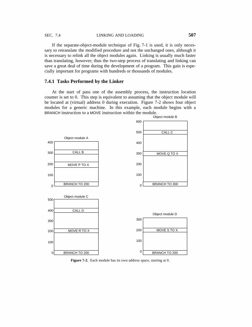
SEC. 7.4 LINKING AND LOADING 507
If the separate-object-module technique of Fig. 7-1 is used, it is only neces-sary to retranslate the modified procedure and not the unchanged ones, although itis necessary to relink all the object modules again. Linking is usually much fasterthan translating, however; thus the two-step process of translating and linking cansave a great deal of time during the development of a program. This gain is espe-cially important for programs with hundreds or thousands of modules.
7.4.1 Tasks Performed by the Linker
At the start of pass one of the assembly process, the instruction locationcounter is set to 0. This step is equivalent to assuming that the object module willbe located at (virtual) address 0 during execution. Figure 7-2 shows four objectmodules for a generic machine. In this example, each module begins with aBRANCH instruction to a MOVE instruction within the module.
Object module A
0
100
200
300
400
BRANCH TO 200
MOVE P TO X
CALL B
0
100
200
300
400
500
600
BRANCH TO 300
MOVE Q TO X
CALL C
Object module B
0
100
200
300
400
500Object module C
BRANCH TO 200
MOVE R TO X
CALL D
0
100
200
300
MOVE S TO X
BRANCH TO 200
Object module D
Figure 7-2. Each module has its own address space, starting at 0.

508 THE ASSEMBLY LANGUAGE LEVEL CHAP. 7
In order to run the program, the linker brings the object modules into mainmemory to form the image of the executable binary program, as shown in Fig. 7-3(a). The idea is to make an exact image of the executable program’s virtualaddress space inside the linker and position all the object modules at their correctlocations. If there is not enough (virtual) memory to form the image, a disk filecan be used. Typically, a small section of memory starting at address zero is usedfor interrupt vectors, communication with the operating system, catching unini-tialized pointers, or other purposes, so programs often start above 0. In this figurewe have (arbitrarily) started programs at address 100.
The program of Fig. 7-3(a), although loaded into the image of the executablebinary file, is not yet ready for execution. Consider what would happen if execu-tion began with the instruction at the beginning of module A. The program wouldnot branch to the MOVE instruction as it should, because that instruction is now at300. In fact, all memory reference instructions will fail for the same reason.
This problem, called the relocation problem, occurs because each objectmodule in Fig. 7-2 represents a separate address space. On a machine with a seg-mented address space, such as the Pentium II, theoretically each object modulecould have its own address space by being placed in its own segment. However,OS/2 is the only operating system for the Pentium II that supports this concept. Allversions of Windows and UNIX support only one linear address space, so all theobject modules must be merged together into a single address space.
Furthermore, the procedure call instructions in Fig. 7-3(a) will not workeither. At address 400, the programmer had intended to call object module B, butbecause each procedure is translated by itself, the assembler has no way of know-ing what address to insert into the CALL B instruction. The address of objectmodule B is not known until linking time. This problem is called the externalreference problem. Both of these problems can be solved by the linker.
The linker merges the separate address spaces of the object modules into asingle linear address space in the following steps:
1. It constructs a table of all the object modules and their lengths.
2. Based on this table, it assigns a starting address to each object module.
3. It finds all the instructions that reference memory adds to each arelocation constant equal to the starting address of its module.
4. It finds all the instructions that reference other procedures and insertsthe address of these procedures in place.
The object module table constructed in step 1 is shown for the modules ofFig. 7-3 below. It gives the name, length, and starting address of each module.
Module Length Starting addressA 400 100B 600 500

SEC. 7.4 LINKING AND LOADING 509
C 500 1100D 300 1600
Figure 7-3(b) shows how the address space of Fig. 7-3(a) looks after the linker hasperformed these steps.
7.4.2 Structure of an Object Module
Object modules often contain six parts, as shown in Fig. 7-4. The first partcontains the name of the module, certain information needed by the linker, such asthe lengths of the various parts of the module, and sometimes the assembly date.
Identification
Entry point table
External reference table
End of module
Machine instructionsand constants
Relocationdictionary
Figure 7-4. The internal structure of an object module produced by a translator.
The second part of the object module is a list of the symbols defined in themodule that other modules may reference, together with their values. For exam-ple, if the module consists of a procedure named bigbug, the entry point table willcontain the character string ‘‘bigbug’’ followed by the address to which itcorresponds. The assembly language programmer indicates which symbols are tobe declared as entry points by using a pseudoinstruction such as PUBLIC inFig. 7-0.
The third part of the object module consists of a list of the symbols that areused in the module but which defined in other modules, along with a list of whichmachine instructions use which symbols. The linker needs the latter list in orderto be able to insert the correct addresses into the instructions that use externalsymbols. A procedure can call other independently translated procedures bydeclaring the names of the called procedures to be external. The assemblylanguage programmer indicates which symbols are to be declared as externalsymbols by using a pseudoinstruction such as EXTERN in Fig. 7-0. On some com-puters entry points and external references are combined into one table.

510 THE ASSEMBLY LANGUAGE LEVEL CHAP. 7
BRANCH TO 200
MOVE P TO X
CALL B
BRANCH TO 300
MOVE Q TO X
CALL C
BRANCH TO 200
MOVE R TO X
CALL D
MOVE S TO X
BRANCH TO 200
1900
1800
1700
1600
1500
1400
1300
1200
1100
1000
900
800
700
600
500
400
300
200
100
ObjectmoduleA
ObjectmoduleB
ObjectmoduleC
ObjectmoduleD
0
BRANCH TO 300
MOVE P TO X
CALL 500
BRANCH TO 800
MOVE Q TO X
CALL 1100
BRANCH TO 1300
MOVE R TO X
CALL 1600
MOVE S TO X
BRANCH TO 1800
1900
1800
1700
1600
1500
1400
1300
1200
1100
1000
900
800
700
600
500
400
300
200
100
ObjectmoduleA
ObjectmoduleB
ObjectmoduleC
ObjectmoduleD
0
Figure 7-3. (a) The object modules of Fig. 7-2 after being positioned in thebinary image but before being relocated and linked. (b) The same objectmodules after linking and after relocation has been performed. Together theyform an executable binary program, ready to run.
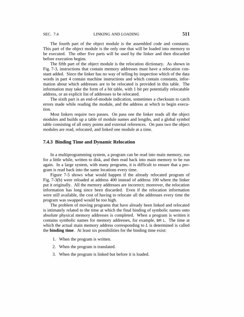
SEC. 7.4 LINKING AND LOADING 511
The fourth part of the object module is the assembled code and constants.This part of the object module is the only one that will be loaded into memory tobe executed. The other five parts will be used by the linker and then discardedbefore execution begins.
The fifth part of the object module is the relocation dictionary. As shown inFig. 7-3, instructions that contain memory addresses must have a relocation con-stant added. Since the linker has no way of telling by inspection which of the datawords in part 4 contain machine instructions and which contain constants, infor-mation about which addresses are to be relocated is provided in this table. Theinformation may take the form of a bit table, with 1 bit per potentially relocatableaddress, or an explicit list of addresses to be relocated.
The sixth part is an end-of-module indication, sometimes a checksum to catcherrors made while reading the module, and the address at which to begin execu-tion.
Most linkers require two passes. On pass one the linker reads all the objectmodules and builds up a table of module names and lengths, and a global symboltable consisting of all entry points and external references. On pass two the objectmodules are read, relocated, and linked one module at a time.
7.4.3 Binding Time and Dynamic Relocation
In a multiprogramming system, a program can be read into main memory, runfor a little while, written to disk, and then read back into main memory to be runagain. In a large system, with many programs, it is difficult to ensure that a pro-gram is read back into the same locations every time.
Figure 7-5 shows what would happen if the already relocated program ofFig. 7-3(b) were reloaded at address 400 instead of address 100 where the linkerput it originally. All the memory addresses are incorrect; moreover, the relocationinformation has long since been discarded. Even if the relocation informationwere still available, the cost of having to relocate all the addresses every time theprogram was swapped would be too high.
The problem of moving programs that have already been linked and relocatedis intimately related to the time at which the final binding of symbolic names ontoabsolute physical memory addresses is completed. When a program is written itcontains symbolic names for memory addresses, for example, BR L. The time atwhich the actual main memory address corresponding to L is determined is calledthe binding time. At least six possibilities for the binding time exist:
1. When the program is written.
2. When the program is translated.
3. When the program is linked but before it is loaded.

512 THE ASSEMBLY LANGUAGE LEVEL CHAP. 7
BRANCH TO 300
MOVE P TO X
CALL 500
BRANCH TO 800
MOVE Q TO X
CALL 1100
BRANCH TO 1300
MOVE R TO X
CALL 1600
MOVE S TO X
BRANCH TO 1800
ObjectmoduleA
ObjectmoduleB
ObjectmoduleC
ObjectmoduleD
1900
1800
1700
1600
1500
1400
1300
1200
1100
1000
900
800
700
600
500
400
0
2000
2100
2200
Figure 7-5. The relocated binary program of Fig. 7-3(b) moved up 300 ad-dresses. Many instructions now refer to an incorrect memory address.

SEC. 7.4 LINKING AND LOADING 513
4. When the program is loaded.
5. When a base register used for addressing is loaded.
6. When the instruction containing the address is executed.
If an instruction containing a memory address is moved after binding, it willbe incorrect (assuming that the object referred to has also been moved). If thetranslator produces an executable binary as output, the binding has occurred attranslation time, and the program must be run at the address the translatorexpected it to be run at. The linking method described in the preceding sectionbinds symbolic names to absolute addresses during linking, which is why movingprograms after linking fails, as shown in Fig. 7-5.
Two related issues are involved here. First, there is the question of whensymbolic names are bound to virtual addresses. Second, there is a question ofwhen virtual addresses are bound to physical addresses. Only when both opera-tions have taken place is binding complete. When the linker merges the separateaddress spaces of the object modules into a single linear address space, it is, infact, creating a virtual address space. The relocation and linking serve to bindsymbolic names onto specific virtual addresses. This observation is true whetheror not virtual memory is being used.
Assume for the moment that the address space of Fig. 7-3(b) were paged. It isclear that the virtual addresses corresponding to the symbolic names A, B, C, andD have already been determined, even though their physical main memoryaddresses will depend on the contents of the page table at the time they are used.An executable binary program is really a binding of symbolic names onto virtualaddresses.
Any mechanism that allows the mapping of virtual addresses onto physicalmain memory addresses to be changed easily will facilitate moving programsaround in main memory, even after they have been bound to a virtual addressspace. One such mechanism is paging. After a program has been moved in mainmemory, only its page table need be changed, not the program itself.
A second mechanism is the use of a runtime relocation register. The CDC6600 and its successors had such a register. On machines using this relocationtechnique, the register always points to the physical memory address of the startof the current program. All memory addresses have the relocation register addedto them by the hardware before being sent to the memory. The entire relocationprocess is transparent to the user programs. They do not even know that it isoccurring. When a program is moved, the operating system must update the relo-cation register. This mechanism is less general than paging because the entireprogram must be moved as a unit (unless there are separate code and data reloca-tion registers, as on the Intel 8088, in which case it has to be moved as two units).
A third mechanism is possible on machines that can refer to memory relativeto the program counter. Whenever a program is moved in main memory only the

514 THE ASSEMBLY LANGUAGE LEVEL CHAP. 7
program counter need be updated. A program, all of whose memory referencesare either relative to the program counter or absolute (e.g., to I/O device registersat absolute addresses) is said to be position independent . A position-independent procedure can be placed anywhere within the virtual address spacewithout the need for relocation.
7.4.4 Dynamic Linking
The linking strategy discussed in Sec. 7.4.1 has the property that all pro-cedures that a program might call are linked before the program can begin execu-tion. On a computer with virtual memory, completing all linking before begin-ning execution does not take advantage of the full capabilities of the virtualmemory. Many programs have procedures that are only called under unusual cir-cumstances. For example, compilers have procedures for compiling rarely usedstatements, plus procedures for handling error conditions that seldom occur.
A more flexible way to link separately compiled procedures is to link eachprocedure at the time it is first called. This process is known as dynamic linking.It was pioneered by MULTICS whose implementation is in some ways still unsur-passed. In the next sections we will look at dynamic linking in several systems.
Dynamic Linking in MULTICS
In the MULTICS form of dynamic linking, associated with each program is asegment, called the linkage segment, which contains one block of information foreach procedure that might be called. This block of information starts with a wordreserved for the virtual address of the procedure and it is followed by the pro-cedure name, which is stored as a character string.
When dynamic linking is being used, procedure calls in the source languageare translated into instructions that indirectly address the first word of thecorresponding linkage block, as shown in Fig. 7-6(a). The compiler fills this wordwith either an invalid address or a special bit pattern that forces a trap.
When a procedure in a different segment is called, the attempt to address theinvalid word indirectly causes a trap to the dynamic linker. The linker then findsthe character string in the word following the invalid address and searches theuser’s file directory for a compiled procedure with this name. That procedure isthen assigned a virtual address, usually in its own private segment, and this virtualaddress overwrites the invalid address in the linkage segment, as indicated inFig. 7-6(b). Next, the instruction causing the linkage fault is reexecuted, allowingthe program to continue from the place it was before the trap.
All subsequent references to that procedure will be executed without causinga linkage fault, for the indirect word now contains a valid virtual address. Conse-quently, the dynamic linker is invoked only the first time a procedure is called andnot thereafter.

SEC. 7.4 LINKING AND LOADING 515
A procedure segment The linkage segment
CALL EARTH
CALL EARTH
CALL FIRE
CALL AIR
CALL WATER
CALL WATER
Indirect
addressingInvalid address
E A R T H
A I R
F I R E
w A T E R
Indirect word
Name of theprocedure isstored as acharacterstring
(a)
(b)
To earth
Linkage informationfor the procedureof AIR
Indirect
addressing
��
Invalid address
���������
Invalid address
�����Invalid address
�A procedure segment The linkage segment
CALL EARTH
CALL EARTH
CALL FIRE
CALL AIR
CALL WATER
CALL WATER
Address of earth
E A R T H
A I R
F I R E
W A T E R
��
Invalid address
Invalid address����Invalid address
���
Figure 7-6. Dynamic linking. (a) Before EARTH is called. (b) After EARTHhas been called and linked.

516 THE ASSEMBLY LANGUAGE LEVEL CHAP. 7
Dynamic Linking in Windows
All versions of the Windows operating system, including NT, support dynamiclinking and rely heavily on it. Dynamic linking uses a special file format called aDLL (Dynamic Link Library). DLLs can contain procedures, data, or both.They are commonly used to allow two or more processes to share library pro-cedures or data. Many DLLs have extension .dll, but other extensions are also inuse, including .drv (for driver libraries) and .fon (for font libraries).
The most common form of a DLL is a library consisting of a collection ofprocedures that can be loaded into memory and accessed by multiple processes atthe same time. Figure 7-7 illustrates two programs sharing a DLL file that con-tains four procedures, A, B, C, and D. Program 1 uses procedure A; program 2uses procedure C, although they could equally well have used the same procedure.
User process 1 User process 2
DLL
Header
A
B
C
D
Figure 7-7. Use of a DLL file by two processes.
A DLL is constructed by the linker from a collection of input files. In fact,building a DLL file is very much like building an executable binary program,except that a special flag is given to the linker to tell it to make a DLL. DLLs arecommonly constructed from collections of library procedures that are likely to beneeded by multiple processes. The interface procedures to the Windows systemcall library and large graphics libraries are common examples of DLLs. Theadvantage of using DLLs is saving space in memory and on disk. If some com-mon library were statically bound to each program using it, it would appear inmany executable binaries on the disk and in memory, wasting space. With DLLs,each library only appears once on disk and once in memory.
In addition to saving space, this approach makes it easy to update library pro-cedures, even after the programs using them have been compiled and linked. For

SEC. 7.4 LINKING AND LOADING 517
commercial software packages, where the users rarely have the source code, usingDLLs means that the software vendor can fix bugs in the libraries by just distri-buting new DLL files over the Internet, without requiring any changes to the mainprogram binaries.
The main difference between a DLL and an executable binary is that a DLLcannot be started and run on its own (because it has no main program). It also hasdifferent information in its header. In addition, the DLL as a whole has severalextra procedures not related to the procedures in the library. For example, there isone procedure that is automatically called whenever a new process is bound to theDLL and another one that is automatically called whenever a process is unboundfrom it. These procedures can allocate and deallocate memory or manage otherresources needed by the DLL.
There are two ways for a program to bind to a DLL. In the first way, calledimplicit linking, the user’s program is statically linked with a special file calledan import library that is generated by a utility program that extracts certaininformation from the DLL. The import library provides the glue that allows theuser program to access the DLL. A user program can be linked with multipleimport libraries. When a program using implicit linking is loaded into memoryfor execution, Windows examines it to see which DLLs it uses and checks to seeif all of them are already in memory. Those that are not in memory are loadedimmediately (but not necessarily in their entirety, since they are paged). Somechanges are then made to the data structures in the import libraries so the calledprocedures can be located, somewhat analogous to the changes shown in Fig. 7-6.They also have to be mapped into the program’s virtual address space. At thispoint, the user program is ready to run and can call the procedures in the DLLs asthough they had been statically bound with it.
The alternative to implicit linking is (not surprisingly) explicit linking. Thisapproach does not require import libraries and does not cause the DLLs to beloaded at the same time the user program is. Instead, the user program makes anexplicit call at run time to bind to a DLL, then makes additional calls to get theaddresses of procedures it needs. Once these have been found, it can call the pro-cedures. When it is all done, it makes a final call to unbind from the DLL. Whenthe last process unbinds from a DLL, the DLL can be removed from memory.
It is important to realize that a procedure in a DLL does not have any identityof its own (as a thread or process does). It runs in the caller’s thread and uses thecaller’s stack for its local variables. It can have process-specific static data (aswell as shared data) and otherwise behaves the same as a statically-linked pro-cedure. The only essential difference is how the binding to it is performed.

518 THE ASSEMBLY LANGUAGE LEVEL CHAP. 7
Dynamic Linking in UNIX
The UNIX system has a mechanism essentially identical in essence to DLLs inWindows. It is called a shared library. Like a DLL file, a shared library is anarchive file containing multiple procedures or data modules that are present inmemory at run time and can be bound to multiple processes at the same time. Thestandard C library and much of the networking code are shared libraries.
UNIX supports only implicit linking, so a shared library consist of two parts: ahost library, which is statically linked with the executable file, and a targetlibrary, which is called at run time. While the details differ, the concepts areessentially the same as with DLLs.

8PARALLEL COMPUTER
ARCHITECTURES
1

CPU
(a)
P P P P
P P P P
P
P
P
P
P
P
P
P
(b)
P P P P
P P P P
P
P
P
P
P
P
P
P
Sharedmemory
Figure 8-1. (a) A multiprocessor with 16 CPUs sharing a com-mon memory. (b) An image partitioned into 16 sections, eachbeing analyzed by a different CPU.

CPU
(a)
P P P P
M M M M
P P P P
M M M M
P
P
P
P
M
M
M
M
P
P
P
P
M
M
M
M
Message-passing
interconnectionnetwork
CPU
(b)
P P P P
P P P P
P
P
P
P
P
P
P
P
Message-passing
interconnectionnetwork
Private memory
Figure 8-2. (a) A multicomputer with 16 CPUs, each witheach own private memory. (b) The bit-map image of Fig. 8-1split up among the 16 memories.

(a)
Machine 1 Machine 2
Languagerun-timesystem
Operatingsystem
Shared memory
Application
Hardware
Languagerun-timesystem
Operatingsystem
Application
Hardware
(b)
Machine 1 Machine 2
Languagerun-timesystem
Operatingsystem
Shared memory
Application
Hardware
Languagerun-timesystem
Operatingsystem
Application
Hardware
(c)
Machine 1 Machine 2
Languagerun-timesystem
Operatingsystem
Shared memory
Application
Hardware
Languagerun-timesystem
Operatingsystem
Application
Hardware
Figure 8-3. Various layers where shared memory can be im-plemented. (a) The hardware. (b) The operating system. (c)The language runtime system.
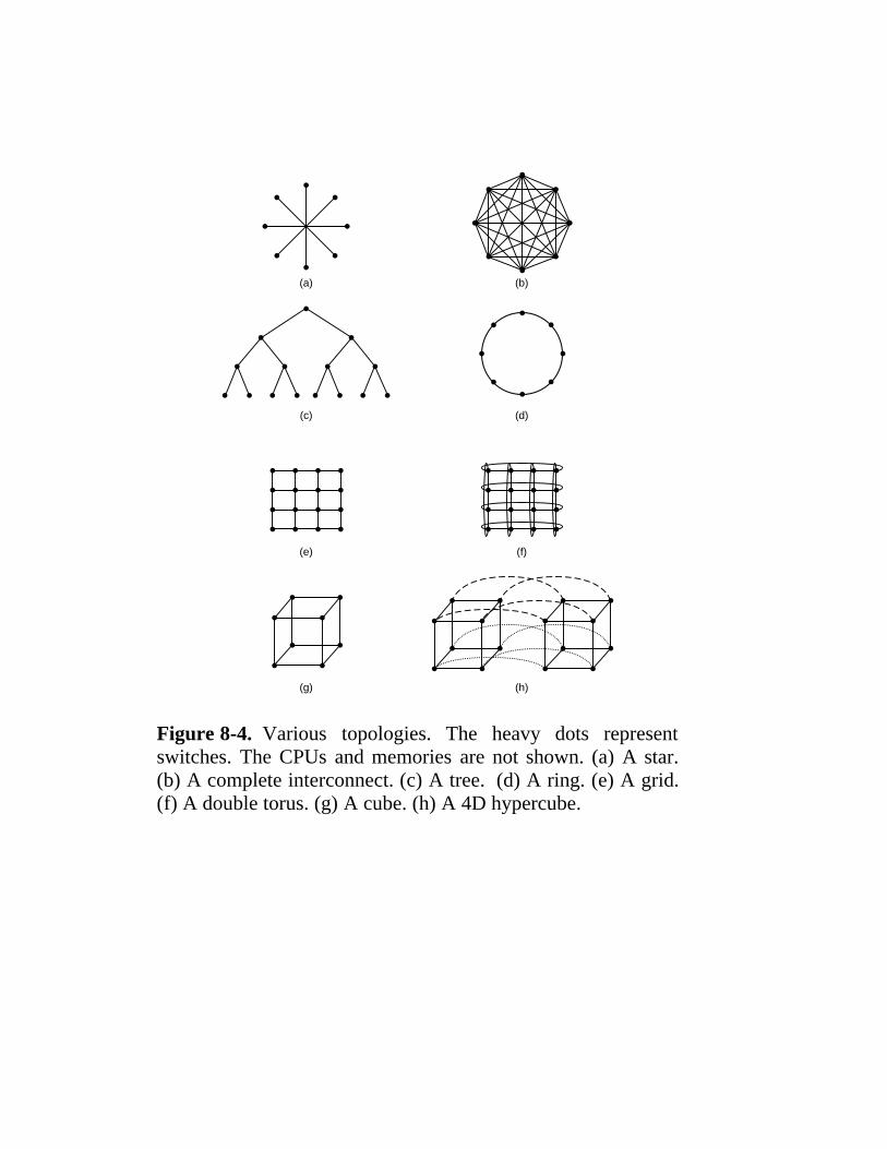
(a)
(c)
(e)
(g)
(b)
(d)
(f)
(h)
Figure 8-4. Various topologies. The heavy dots representswitches. The CPUs and memories are not shown. (a) A star.(b) A complete interconnect. (c) A tree. (d) A ring. (e) A grid.(f) A double torus. (g) A cube. (h) A 4D hypercube.

CPU 1
Endof
packet
Middleof
packet
A
Input port
Output port
Front of packet
Four-port switch
B
C D
CPU 2
Figure 8-5. An interconnection network in the form of a four-switch square grid. Only two of the CPUs are shown.

CPU 1 Input port
(a)
Output port
Entirepacket
Entirepacket
Four-portswitch
C
A
CPU 2
Entirepacket
D
B
(b)
C
A
D
B
(c)
C
A
D
B
Figure 8-6. Store-and-forward packet switching.
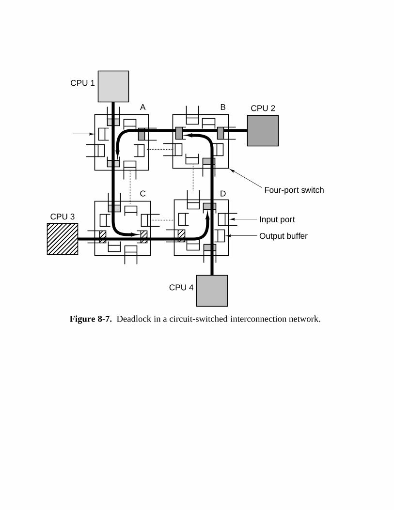
CPU 1
CPU 2
CPU 3
A
C
B
D
Input port
Output buffer
Four-port switch
CPU 4
���� �����������
Figure 8-7. Deadlock in a circuit-switched interconnection network.
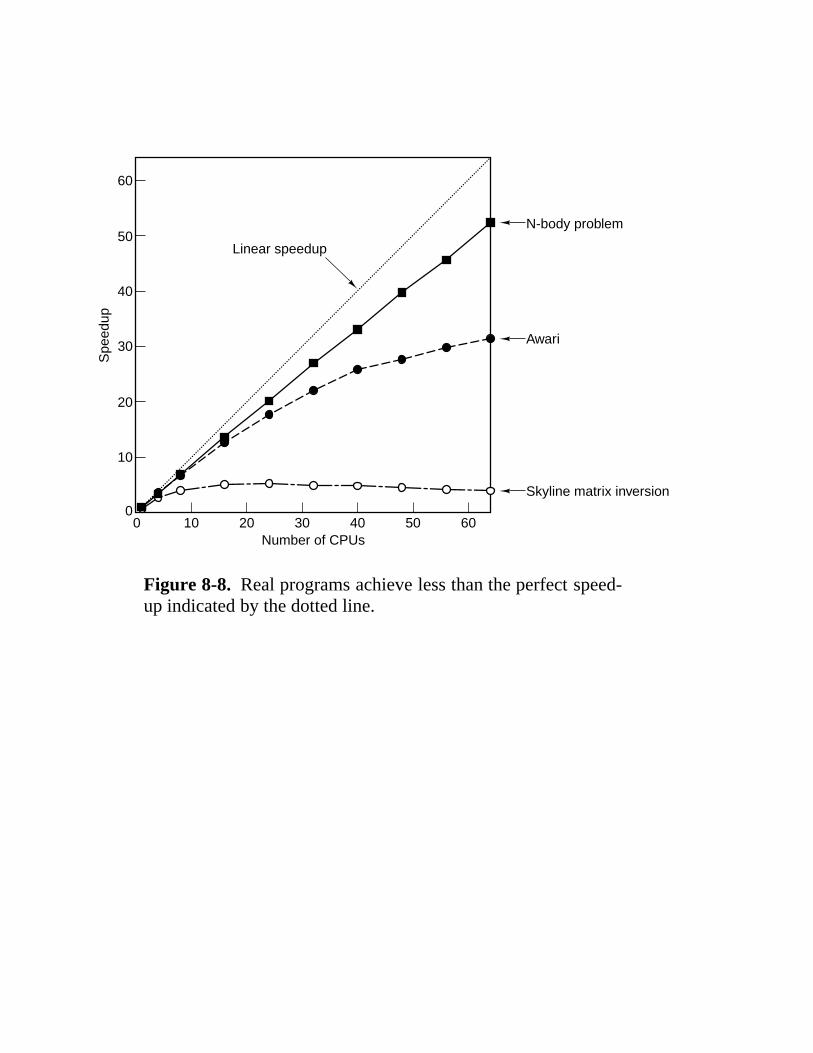
6050403020100
60
50
40
30
20
10
0
Spe
edup
Linear speedup
N-body problem
Awari
Skyline matrix inversion
Number of CPUs
Figure 8-8. Real programs achieve less than the perfect speed-up indicated by the dotted line.

(a)
n CPUs active
1 CPUactive
1 – ff
T
Inherentlysequential
part
(b)
1 – ff
Potentiallyparallelizable
part
…
fT (1 – f)T/n
Figure 8-9. (a) A program has a sequential part and a parallel-izable part. (b) Effect of running part of the program in paral-lel.

CPU
Bus
(a) (b) (c) (d)
Figure 8-10. (a) A 4-CPU bus-based system. (b) A 16-CPUbus-based system. (c) A 4-CPU grid-based system. (d) A 16-CPU grid-based system.
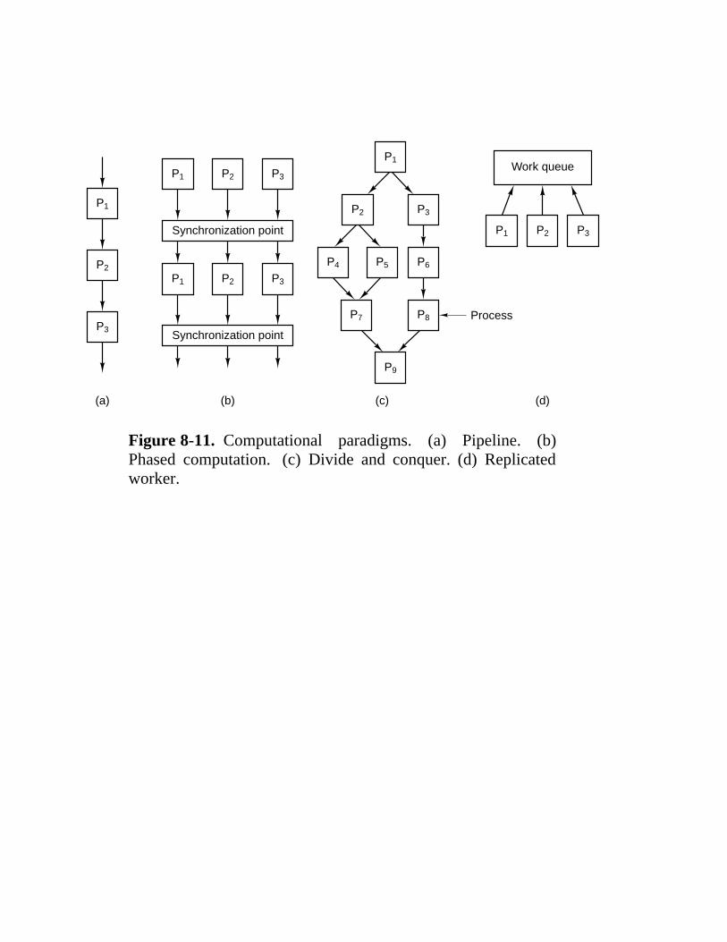
Process
P1
(d)
P2
P5 P6
P3
P2P1 P3
P8P7
P1
P9
P1
P2
P3
P2 P3
Synchronization point
P1 P2 P3
Synchronization point
P4
Work queue
(c)(b)(a)
Figure 8-11. Computational paradigms. (a) Pipeline. (b)Phased computation. (c) Divide and conquer. (d) Replicatedworker.

222222222222222222222222222222222222222222222222222222222222222222222222222222222222Physical
(hardware)Logical
(software) Examples222222222222222222222222222222222222222222222222222222222222222222222222222222222222Multiprocessor Shared variables Image processing as in Fig. 8-1222222222222222222222222222222222222222222222222222222222222222222222222222222222222Multiprocessor Message passing Message passing simulated with buffers in memory222222222222222222222222222222222222222222222222222222222222222222222222222222222222Multicomputer Shared variables DSM, Linda, Orca, etc. on an SP/2 or a PC network222222222222222222222222222222222222222222222222222222222222222222222222222222222222Multicomputer Message passing PVM or MPI on an SP/2 or a network of PCs222222222222222222222222222222222222222222222222222222222222222222222222222222222222111111111
111111111
111111111
111111111
Figure 8-12. Combinations of physical and logical sharing.

2222222222222222222222222222222222222222222222222222222222222222222222222Instructionstreams
Datastreams Name Examples2222222222222222222222222222222222222222222222222222222222222222222222222
1 1 SISD Classical Von Neumann machine22222222222222222222222222222222222222222222222222222222222222222222222221 Multiple SIMD Vector supercomputer, array processor2222222222222222222222222222222222222222222222222222222222222222222222222Multiple 1 MISD Arguably none2222222222222222222222222222222222222222222222222222222222222222222222222Multiple Multiple MIMD Multiprocessor, multicomputer2222222222222222222222222222222222222222222222222222222222222222222222222111111111
111111111
111111111
111111111
111111111
Figure 8-13. Flynn’s taxonomy of parallel computers.

SISD
(Von Neumann)
SIMD
Parallel computer architectures
MISD
?
MIMD
Vectorprocessor
Arrayprocessor
Multi-processors
Multi-computers
UMA COMA NUMA MPP COW
Bus Switched CC-NUMA NC-NUMA GridHyper-cube
Shared memory Message passing
Figure 8-14. A taxonomy of parallel computers.
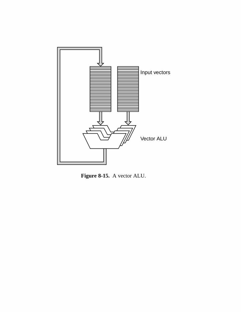
Input vectors
Vector ALU
Figure 8-15. A vector ALU.

222222222222222222222222222222222222222222222222Operation Examples222222222222222222222222222222222222222222222222
Ai = f1(Bi) f1 = cosine, square root222222222222222222222222222222222222222222222222Scalar = f2(A) f2 = sum, minimum222222222222222222222222222222222222222222222222Ai = f3(Bi, Ci) f3 = add, subtract222222222222222222222222222222222222222222222222Ai = f4(scalar,Bi) f4 = multiply Bi by a constant22222222222222222222222222222222222222222222222211
111111
11111111
11111111
Figure 8-16. Various combinations of vector and scalar operations.

222222222222222222222222222222222222222222222222222222222Step Name Values222222222222222222222222222222222222222222222222222222222
1 Fetch operands 1.082 × 10¹² − 9.212 × 10112222222222222222222222222222222222222222222222222222222222 Adjust exponent 1.082 × 10¹² − 0.9212 × 10122222222222222222222222222222222222222222222222222222222223 Execute subtraction 0.1608 × 10122222222222222222222222222222222222222222222222222222222224 Normalize result 1.608 × 101122222222222222222222222222222222222222222222222222222222211
111111
11111111
11111111
11111111
Figure 8-17. Steps in a floating-point subtraction.

222222222222222222222222222222222222222222222222222222222222222222222222222222Cycle222222222222222222222222222222222222222222222222222222222222222222222222222222
Step 1 2 3 4 5 6 7222222222222222222222222222222222222222222222222222222222222222222222222222222Fetch operands B1, C1 B2, C2 B3, C3 B4, C4 B5, C5 B6, C6 B7, C7222222222222222222222222222222222222222222222222222222222222222222222222222222Adjust exponent B1, C1 B2, C2 B3, C3 B4, C4 B5, C5 B6, C6222222222222222222222222222222222222222222222222222222222222222222222222222222Execute operation B1 + C1 B2 + C2 B3 + C3 B4 + C4 B5 + C5222222222222222222222222222222222222222222222222222222222222222222222222222222Normalize result B1 + C1 B2 + C2 B3 + C3 B4 + C4222222222222222222222222222222222222222222222222222222222222222222222222222222111111111
111111111
11111111
11111111
11111111
11111111
11111111
11111111
111111111
Figure 8-18. A pipelined floating-point adder.

A B S T
ADD
Address units
824-Bitaddressregisters
6424-Bitholdingregistersforaddresses
864-Bitscalarregisters
6464-Bit holdingregisters forscalars
64 Elementsper register
8 64-Bitvector registers
Scalarinteger units
Scalar/vectorfloatng-pointunits
Vectorintegerunits
ADD
BOOLEAN
SHIFT
ADD
MUL
RECIP.
ADD
BOOLEAN
SHIFT
POP. COUNT
MUL
Figure 8-19. Registers and functional units of the Cray-1
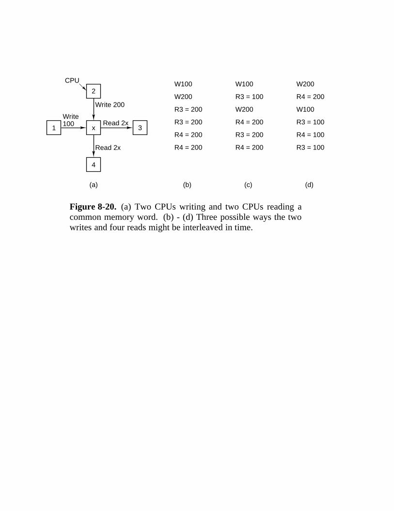
CPU
Write100
Write 200
Read 2x
Read 2x
(a) (b)
W100
W200
R3 = 200
R3 = 200
R4 = 200
R4 = 200
(c)
W100
R3 = 100
W200
R4 = 200
R3 = 200
R4 = 200
(d)
W200
R4 = 200
W100
R3 = 100
R4 = 100
R3 = 100
1
2
3
4
x
Figure 8-20. (a) Two CPUs writing and two CPUs reading acommon memory word. (b) - (d) Three possible ways the twowrites and four reads might be interleaved in time.

CPU A
CPU B
CPU C
Write
1A 1B
2A
1C
2B
3A 3B
1D 1E
2C
3C
1F
2D
Time
Synchronization point
Figure 8-21. Weakly consistent memory uses synchronizationoperations to divide time into sequential epochs.

Shared memory
CPU M
Bus
(a) (b) (c)
Cache
Private memory Sharedmemory
CPU CPU MCPU CPU MCPU
Figure 8-22. Three bus-based multiprocessors. (a) Withoutcaching. (b) With caching. (c) With caching and privatememories.

22222222222222222222222222222222222222222222222222222222222222Action Local request Remote request22222222222222222222222222222222222222222222222222222222222222
Read miss Fetch data from memory22222222222222222222222222222222222222222222222222222222222222Read hit Use data from local cache22222222222222222222222222222222222222222222222222222222222222Write miss Update data in memory22222222222222222222222222222222222222222222222222222222222222Write hit Update cache and memory Invalidate cache entry2222222222222222222222222222222222222222222222222222222222222211
111111
11111111
11111111
11111111
Figure 8-23. The write through cache coherence protocol.The empty boxes indicate that no action is taken.

(a)
(b)
(c)
(d)
(e)
(f)
Exclusive
Cache Bus
Bus
Bus
Bus
Bus
Bus
Shared Shared
Shared Shared
Modified
Modified
Modified
CPU 1 reads block A
CPU 2 reads block A
CPU 2 writes block A
CPU 3 reads block A
CPU 2 writes block A
CPU 1 writes block A
CPU 1 CPU 2 CPU 3Memory
CPU 1 CPU 2 CPU 3Memory
CPU 1 CPU 2 CPU 3Memory
CPU 1 CPU 2 CPU 3Memory
CPU 1 CPU 2 CPU 3Memory
CPU 1 CPU 2 CPU 3Memory
A
A
A
A
A
A
A
Figure 8-24. The MESI cache coherence protocol.

Memories
CP
Us
Closedcrosspointswitch
Opencrosspointswitch
(a)
(b)
(c)
Crosspointswitch is closed
Crosspointswitch is open
000
001
010
011
100
101
110
111
100
101
110
111
000
001
010
011
Figure 8-25. (a) An 8 × 8 crossbar switch. (b) An opencrosspoint. (c) A closed crosspoint.

Transfer unit is64-bytecache block
Boardhad 4 GB +4 CPUs
Fouraddressbuses forsnooping
UltraSPARC CPU
1-GB memorymodule
0 1 2 14 15
16 × 16 Crossbar switch (Gigaplane-XB)
…
Figure 8-26. The Sun Enterprise 10000 symmetric multiprocessor.

A
B
X
Y
(a) (b)
Module Address Opcode Value
Figure 8-27. (a) A 2 × 2 switch. (b) A message format.

CPUs
b
b
bb
a
a a
a
3 Stages
Memories
000
001
010
011
100
101
110
111
000
001
010
011
100
101
110
111
1A
1B
1C
1D
2A
2B
2C
2D
3A
3B
3C
3D
Figure 8-28. An omega switching network.

System bus
CPU
MMU
Memory
Local bus
CPU Memory
Local bus
CPU Memory
Local bus
CPU Memory
Local bus
Figure 8-29. A NUMA machine based on two levels of buses.The Cm* was the first multiprocessor to use this design.

Directory
Node 0 Node 1 Node 255
(a)
(b)
Bits 8 18 6
(c)
Interconnection network
CPU Memory
Local bus
CPU Memory
Local bus
CPU Memory
Local bus
Node Block Offset
01234
00100
218-1
82
…
Figure 8-30. (a) A 256-node directory-based multiprocessor.(b) Division of a 32-bit memory address into fields. (c) Thedirectory at node 36.
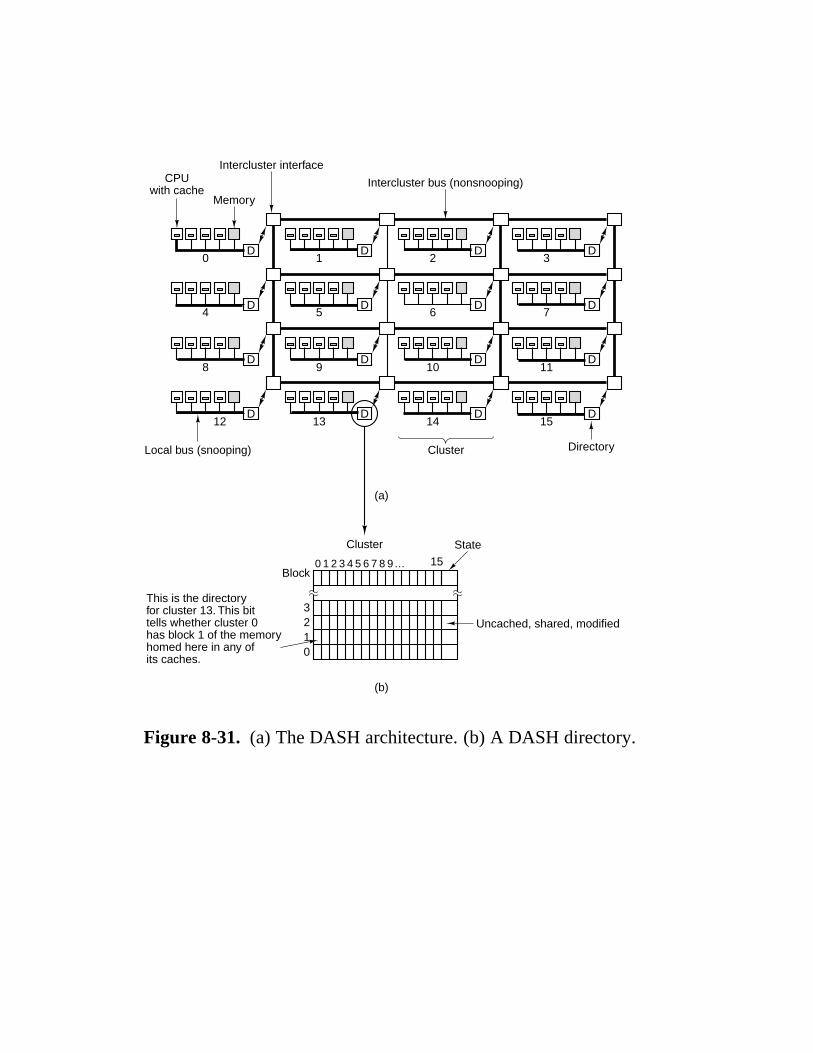
CPUwith cache
Memory
Intercluster interface
Intercluster bus (nonsnooping)
0
4
8
12
Local bus (snooping)
13
9
5
1 2 3
7
11
15
6
10
14
(a)
(b)
Cluster Directory
Cluster
Block
State
… 15
Uncached, shared, modified
This is the directoryfor cluster 13. This bittells whether cluster 0has block 1 of the memoryhomed here in any ofits caches.
0123
D D D D
D D D D
D D D D
D D D D
0 1 2 3 4 5 6 7 8 9
Figure 8-31. (a) The DASH architecture. (b) A DASH directory.

Snooping bus interfaceDirectory controller
IQ board
Data pump
RAM CPU
SCI ring
Directory32-MB cache RAM
Quad board with4 Pentium Pros andup to 4 GB of RAM
Figure 8-32. The NUMA-Q multiprocessor.

Local memory tableat home node
Bits 6 7 13 6
0
219-1Back State Tag Fwd
Node 4 cache directory Node 9 cache directory Node 22 cache directory
Back State Tag Fwd Back State Tag Fwd
Figure 8-33. SCI chains all the holders of a given cache linetogether in a doubly-linked list. In this example, a line isshown cached at three nodes.

……
CPU MemoryNode
Communicationprocessor
Local interconnectDiskandI/O
…Local interconnect
DiskandI/O
High-performance interconnection network
Figure 8-34. A generic multicomputer.

GigaRing
Shell
Node
…
Alpha
Control +E registers
Commun.processor
Mem
Full-duplex 3D torus
Alpha
Control +E registers
Commun.processor
Mem
Network Disk Tape
Alpha
Control +E registers
Commun.processor
Mem
Figure 8-35. The Cray Research T3E.

(a) (b)
64-Bit local bus
64-Bit local bus
PPro 64MB
Kestrelboard
2
I/O NICPPro
PPro 64MB I/O NICPPro
32
38
Figure 8-36. The Intel/Sandia Option Red system. (a) Thekestrel board. (b) The interconnection network.

CPU group
0 1 2 3 4 5 6 7
Tim
e
(a) (b) (c)
CPU group
0 1 2 3 4 5 6 7
CPU group
0 1 2 3 4 5 6 7
1
2
3
4 5
6
7
8 9
1
2
3
4
5
6
7
8
9
1
2
3
4
5
6
7
8
9
Figure 8-37. Scheduling a COW. (a) FIFO. (b) Without head-of-line blocking. (c) Tiling. The shaded areas indicate idleCPUs.

CPU CPU CPU
Packetgoing east
Packetgoing west
(a) (b)
Line cardEthernet
Switch
Back-plane
Figure 8-38. (a) Three computers on an Ethernet. (b) An Eth-ernet switch.
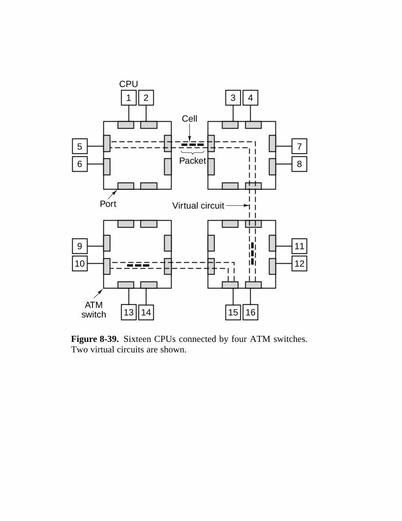
CPU
ATMswitch
Port
Cell
Packet
Virtual circuit
1 2 3 4
5
6
7
8
9
10
11
12
13 14 15 16
Figure 8-39. Sixteen CPUs connected by four ATM switches.Two virtual circuits are shown.

Globally shared virtual memory consisting of 16 pages
Memory
Network(a)
(b)
(c)
0 1 2 3 4 5 6 7 8 9 10 11 12 13 14 15
CPU 0
0 2 5
9
CPU 1
1 3 6
8 10
CPU 2
4 7 11
12 14
CPU 3
13 15
CPU 0
0 2 5
9
CPU 1
1 3 6
810
10
CPU 2
4 7 11
12 14
CPU 3
13 15
CPU 0
0 2 5
9
CPU 1
1 3 6
8 10
CPU 2
4 7 11
12 14
CPU 3
13 15
Figure 8-40. A virtual address space consisting of 16 pagesspread over four nodes of a multicomputer. (a) The initial situa-tion. (b) After CPU 0 references page 10. (c) After CPU 1references page 10, here assumed to be a read-only page.

(′′abc′′, 2, 5)(′′matrix-1′′, 1, 6, 3.14)(′′family′′, ′′is sister′′, Carolyn, Elinor)
Figure 8-41. Three Linda tuples.

Object implementation stack;top:integer; # storage for the stackstack: array [integer 0..N-1] of integer;
operation push(item: integer); function returning nothingbegin
stack[top] := item; push item onto the stacktop := top + 1; # increment the stack pointer
end;
operation pop( ): integer; # function returning an integerbegin
guard top > 0 do # suspend if the stack is emptytop := top - 1; # decrement the stack pointerreturn stack[top]; # return the top item
od;end;
begintop := 0; # initialization
end;
Figure 8-42. A simplified ORCA stack object, with internal dataand two operations.

524 PARALLEL COMPUTER ARCHITECTURES CHAP. 8
8.1 DESIGN ISSUES FOR PARALLEL COMPUTERS
When approaching a new parallel computer system, three fundamental ques-tions to ask are
1. What are the nature, size, and number of the processing elements?
2. What are the nature, size, and number of the memory modules?
3. How are the processing and memory elements interconnected?
Let us examine each of these points briefly in turn. The processing elements canrange from minimal ALUs through complete CPUs, with sizes ranging from asmall portion of a chip to a cubic meter of electronics per element. As one mightexpect, when the processing element is a fraction of a chip, it is possible to equipa computer with vast numbers, perhaps even a million of such elements. Whenthe processing element is a complete computer, with its own memory and I/Oequipment, the sizes are smaller, naturally, although systems with almost 10,000CPUs have been installed. More and more, parallel computers are being con-structed from commercially available parts, especially CPUs. The capabilitiesand limitations of these parts often heavily influence the design.
Memory systems are often split up into modules that operate independently ofone another, in parallel to allow access by many CPUs at the same time. Thesemodules can be small (kilobytes) or large (megabytes) and closely integrated withthe CPUs or located on a different circuit board. Since large dynamic memories(DRAMs) are usually much slower than CPUs, elaborate caching schemes are fre-quently used to speed up memory access. Often two, three, and even four levelsof caching are used.
Although there is some variation among CPU and memory designs, the areain which parallel systems differ most is how the pieces are put together. Theinterconnection schemes can be divided into two rough categories: static anddynamic. The static ones simply wire up all the components in a fixed way, suchas a star, ring, or grid. In dynamic interconnection schemes, all the pieces arehooked up to a switching network that can dynamically route messages betweencomponents. Each has its own strengths and weaknesses, as we shall soon see.
Viewing parallel computers as a collection of chips that are wired up in onemanner or another is essentially a bottom-up view of the world. In a top-downapproach, one would ask: ‘‘What is it that is to be run in parallel?’’ Here again, wehave a spectrum of possibilities. Some parallel computers are designed to runmultiple independent jobs simultaneously. These jobs have nothing to do withone another and do not communicate. A typical example is a computer with 8 to64 CPUs intended as a big UNIX timesharing system for handling thousands ofremote users. Transaction processing systems used by banks (e.g., automatedteller machines), airlines (e.g., reservation systems) and large Web servers alsofall into this category, as do independent simulation runs using different sets of

SEC. 8.1 DESIGN ISSUES FOR PARALLEL COMPUTERS 525
parameters.A different point on this spectrum is the parallel computer used for running a
single job consisting of many parallel processes. As an example, consider a chessprogram that analyzes a given board by generating a list of legal moves that canbe made from it, and then forking off parallel processes to (recursively) analyzeeach new board in parallel. The point of the parallelism here is not to accommo-date more users, but to gain speedup on a single problem.
Continuing along this spectrum, we come to machines in which the parallel-ism comes from a high degree of pipelining or many ALUs operating on the sameinstruction stream at the same time. Numeric supercomputers with specialhardware for vector processing fall in this category. Here we not only have onemain problem being solved, but all parts of the computer are working very closelyon almost the same aspect of the problem together (e.g., different elements of thesame two vectors are being added in parallel).
Although it is hard to pin down exactly, these three examples differ in what issometimes called grain size. In the multi-CPU timesharing systems, the unit ofparallelism is large: a complete user program. Running large pieces of softwarein parallel with little or no communication between the pieces is called coarse-grained parallelism. The opposite extreme, such as found in vector processing,is called fine-grained parallelism.
Grain size refers to the algorithms and software, but it has a direct analog inthe hardware. Systems with a small number of large, independent CPUs that havelow-speed connections between the CPUs are called loosely coupled. Theiropposite number are the tightly-coupled systems, in which the components aregenerally smaller, closer together and interact with each other frequently overhigh-bandwidth communication networks. In most cases, problems with coarse-grained parallelism work best on loosely-coupled systems; Similarly, problemswith fine-grained parallelism work best on tightly-coupled systems. However, somuch variety exists in algorithms, software, and hardware, that this is a generalguide at best. The wide range in problem grain size and possibilities for systemcoupling have led to the wide variety of architectures that we will study in thischapter.
In the following sections we will examine some of the design issues for paral-lel computers, starting with communication models and interconnection networks.Then we will look at performance and software issues. Finally, we will concludewith a taxonomy of parallel computer architectures that will guide the organiza-tion of the rest of this chapter.
8.1.1 Communication Models
In any parallel computer system, CPUs working on different parts of the samejob must communicate with one another to exchange information. Precisely howthey should do this is the subject of much debate in the architectural community.
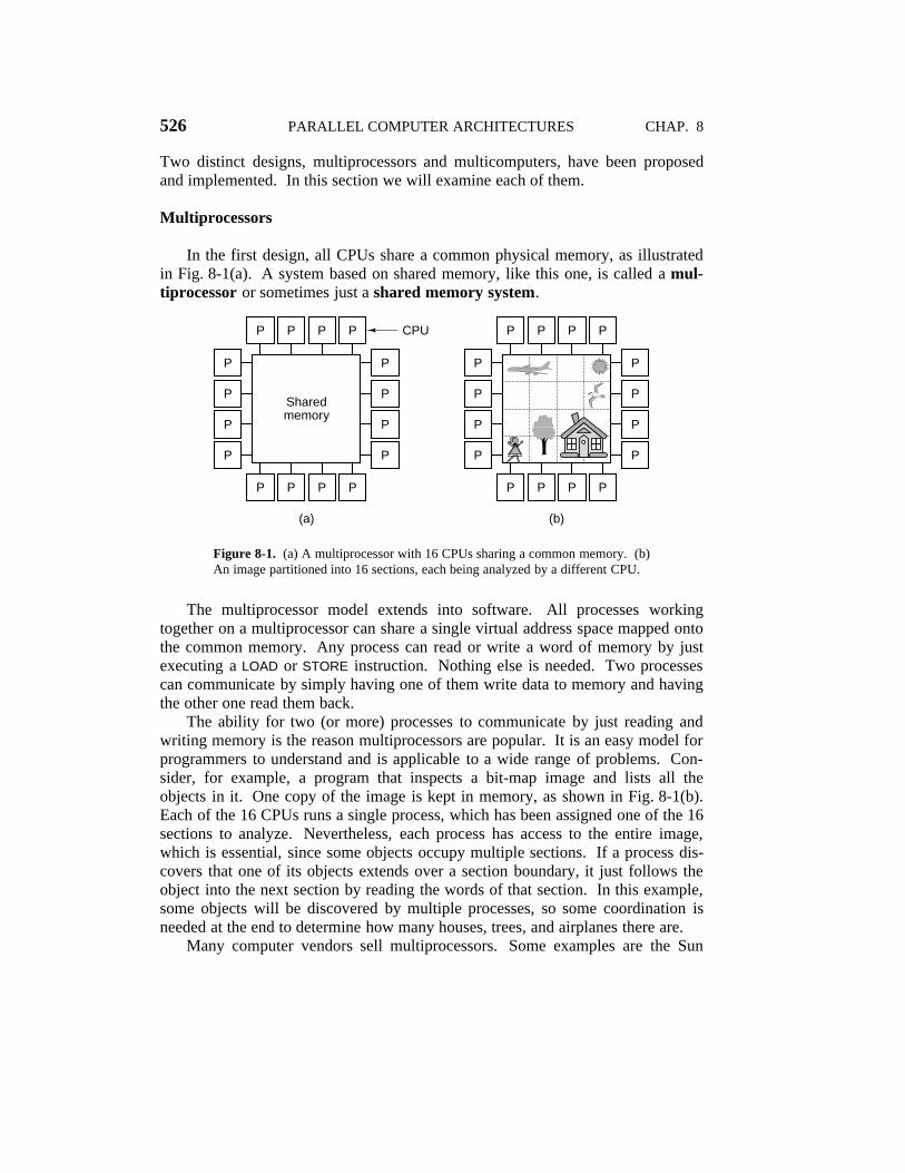
526 PARALLEL COMPUTER ARCHITECTURES CHAP. 8
Two distinct designs, multiprocessors and multicomputers, have been proposedand implemented. In this section we will examine each of them.
Multiprocessors
In the first design, all CPUs share a common physical memory, as illustratedin Fig. 8-1(a). A system based on shared memory, like this one, is called a mul-tiprocessor or sometimes just a shared memory system.
CPU
(a)
P P P P
P P P P
P
P
P
P
P
P
P
P
(b)
P P P P
P P P P
P
P
P
P
P
P
P
P
Sharedmemory
Figure 8-1. (a) A multiprocessor with 16 CPUs sharing a common memory. (b)An image partitioned into 16 sections, each being analyzed by a different CPU.
The multiprocessor model extends into software. All processes workingtogether on a multiprocessor can share a single virtual address space mapped ontothe common memory. Any process can read or write a word of memory by justexecuting a LOAD or STORE instruction. Nothing else is needed. Two processescan communicate by simply having one of them write data to memory and havingthe other one read them back.
The ability for two (or more) processes to communicate by just reading andwriting memory is the reason multiprocessors are popular. It is an easy model forprogrammers to understand and is applicable to a wide range of problems. Con-sider, for example, a program that inspects a bit-map image and lists all theobjects in it. One copy of the image is kept in memory, as shown in Fig. 8-1(b).Each of the 16 CPUs runs a single process, which has been assigned one of the 16sections to analyze. Nevertheless, each process has access to the entire image,which is essential, since some objects occupy multiple sections. If a process dis-covers that one of its objects extends over a section boundary, it just follows theobject into the next section by reading the words of that section. In this example,some objects will be discovered by multiple processes, so some coordination isneeded at the end to determine how many houses, trees, and airplanes there are.
Many computer vendors sell multiprocessors. Some examples are the Sun

SEC. 8.1 DESIGN ISSUES FOR PARALLEL COMPUTERS 527
Enterprise 10000, Sequent NUMA-Q, SGI Origin 2000, and HP/Convex Exem-plar.
Multicomputers
The second design for a parallel architecture is one in which each CPU has itsown private memory, accessible only to itself and not to any other CPU. Such adesign is called a multicomputer, or sometimes a distributed memory system,and is illustrated in Fig. 8-2(a). Multicomputers are frequently (but not always)loosely coupled. The key aspect of a multicomputer that distinguishes it from amultiprocessor is that each CPU in a multicomputer has its own private, localmemory that it can access by just executing LOAD and STORE instructions, butwhich no other CPU can access using LOAD and STORE instructions. Thus mul-tiprocessors have a single physical address space shared by all the CPUs whereasmulticomputers have one physical address space per CPU.
Since the CPUs on a multicomputer cannot communicate by just reading andwriting the common memory, they need a different communication mechanism.What they do is pass messages back and forth using the interconnection network.Examples of multicomputers include the IBM SP/2, Intel/Sandia Option Red, andthe Wisconsin COW.
CPU
(a)
P P P P
M M M M
P P P P
M M M M
P
P
P
P
M
M
M
M
P
P
P
P
M
M
M
M
Message-passing
interconnectionnetwork
CPU
(b)
P P P P
P P P P
P
P
P
P
P
P
P
P
Message-passing
interconnectionnetwork
Private memory
Figure 8-2. (a) A multicomputer with 16 CPUs, each with each own privatememory. (b) The bit-map image of Fig. 8-1 split up among the 16 memories.
The absence of hardware shared memory on a multicomputer has importantimplications for the software structure. Having a single virtual address space withall processes being able to read and write all of memory by just executing LOAD

528 PARALLEL COMPUTER ARCHITECTURES CHAP. 8
and STORE instructions is impossible on a multicomputer. For example, if CPU 0(the one in the upper left-hand corner) of Fig. 8-1(b) discovers that part of itsobject extends into the section assigned to CPU 1, it can nevertheless just con-tinue reading memory to access the nose of the airplane. On the other hand, ifCPU 0 in Fig. 8-2(b) makes the same discovery, it cannot just read CPU 1’smemory. It has to do something quite different to get the data it needs.
In particular, it has to discover (somehow) which CPU has the data it needsand send that CPU a message requesting a copy of the data. Typically it will thenblock (i.e., wait) until the request is answered. When the message arrives at CPU1, software there has to analyze it and send back the needed data. When the replymessage gets back to CPU 0, the software is unblocked and can continue execut-ing.
On a multicomputer, communication between processes often uses softwareprimitives such as send and receive. This gives the software a different, and farmore complicated structure, than on a multiprocessor. It also means that correctlydividing up the data and placing them in the optimal locations is a major issue ona multicomputer. It is less of an issue on a multiprocessor since placement doesnot affect correctness or programmability although it may affect performance. Inshort, programming a multicomputer is much more difficult than programming amultiprocessor.
Under these conditions, why would anyone build multicomputers, when mul-tiprocessors are easier to program? The answer is simple: large multicomputersare much simpler and cheaper to build than multiprocessors with the same numberof CPUs. Implementing a memory shared by even a few hundred CPUs is a sub-stantial undertaking, whereas building a multicomputer with 10,000 CPUs ormore is straightforward.
Thus we have a dilemma: multiprocessors are hard to build but easy to pro-gram whereas multicomputers are easy to build but hard to program. This obser-vation has led to a great deal of effort to construct hybrid systems that are rela-tively easy to build and relatively easy to program. This work has led to the reali-zation that shared memory can be implemented in various ways, each with its ownset of advantages and disadvantages. In fact, much of the research in parallelarchitectures these days relates to the convergence of multiprocessor and multi-computer architectures into hybrid forms that combine the strengths of each. Theholy grail here is to find designs that are scalable, that is, continue to performwell as more and more CPUs are added.
One approach to building hybrid systems is based on the fact that moderncomputer systems are not monolithic but are constructed as a series of layers—thetheme of this book. This insight opens the possibility of implementing the sharedmemory at any one of several layers, as shown in Fig. 8-3. In Fig. 8-3(a) we seethe shared memory being implemented by the hardware as a true multiprocessor.In this design, there is a single copy of the operating system with a single set oftables, in particular, the memory allocation table. When a process needs more

SEC. 8.1 DESIGN ISSUES FOR PARALLEL COMPUTERS 529
memory, it traps to the operating system, which then looks in its table for a freepage and maps the page into the caller’s address space. As far as the operatingsystem is concerned, there is a single memory and it keeps track of which processowns which page in software. There are many ways to implement hardwareshared memory, as we will see later.
(a)
Machine 1 Machine 2
Languagerun-timesystem
Operatingsystem
Shared memory
Application
Hardware
Languagerun-timesystem
Operatingsystem
Application
Hardware
(b)
Machine 1 Machine 2
Languagerun-timesystem
Operatingsystem
Shared memory
Application
Hardware
Languagerun-timesystem
Operatingsystem
Application
Hardware
(c)
Machine 1 Machine 2
Languagerun-timesystem
Operatingsystem
Shared memory
Application
Hardware
Languagerun-timesystem
Operatingsystem
Application
Hardware
Figure 8-3. Various layers where shared memory can be implemented. (a) Thehardware. (b) The operating system. (c) The language runtime system.
A second possibility is to use multicomputer hardware and have the operatingsystem simulate shared memory by providing a single system-wide paged sharedvirtual address space. In this approach, called DSM (Distributed SharedMemory) (Li, 1988; and Li and Hudak, 1986, 1989), each page is located in oneof the memories of Fig. 8-2(a). Each machine has its own virtual memory and itsown page tables. When a CPU does a LOAD or STORE on a page it does not have,a trap to the operating system occurs. The operating system then locates the pageand asks the CPU currently holding it to unmap the page and send it over theinterconnection network. When it arrives, the page is mapped in and the faultinginstruction is restarted. In effect, the operating system is just satisfying pagefaults from remote memory instead of from disk. To the user, the machine looksas if it has shared memory. We will examine DSM later in this chapter.

530 PARALLEL COMPUTER ARCHITECTURES CHAP. 8
A third possibility is to have a user-level runtime system implement a (possi-bly language-specific) form of shared memory. In this approach, the program-ming language provides some kind of shared memory abstraction, which is thenimplemented by the compiler and runtime system. For example, the Linda modelis based on the abstraction of a shared space of tuples (data records containing acollection of fields). Processes on any machine can input a tuple from the sharedtuple space or output a tuple to the shared tuple space. Because access to thetuple space is controlled entirely in software (by the Linda runtime system), nospecial hardware or operating system support is needed.
Another example of a language-specific shared memory implemented by theruntime system is the Orca model of shared data objects. In Orca, processes sharegeneric objects rather than just tuples and can execute object-specific methods onthem. When a method changes the internal state of an object, it is up to the run-time system to make sure all copies of the object on all machines are simultane-ously updated. Again, because objects are a strictly software concept, the imple-mentation can be done by the runtime system help from the operating system orhardware. We will look at both Linda and Orca later in this chapter.
8.1.2 Interconnection Networks
In Fig. 8-2 we saw that multicomputers are held together by interconnectionnetworks. Now it is time to look more closely at these interconnection networks.Interestingly enough, multiprocessors and multicomputers are surprisingly similarin this respect because multiprocessors often have multiple memory modules thatmust also be interconnected with one another and with the CPUs. Thus thematerial in this section frequently applies to both kinds of systems.
The fundamental reason why multiprocessor and multicomputer interconnec-tion networks are similar is that at the very bottom both of them use messagepassing. Even on a single-CPU machine, when the processor wants to read orwrite a word, what it typically does is assert certain lines on the bus and wait for areply. This action is fundamentally like message passing: the initiator sends arequest and waits for a response. In large multiprocessors, communicationbetween CPUs and remote memory almost always consists of the CPU sending anexplicit message, called a packet, to memory requesting some data, and thememory sending back a reply packet.
Interconnection networks can consist of up to five components:
1. CPUs
2. Memory modules.
3. Interfaces.
4. Links.

SEC. 8.1 DESIGN ISSUES FOR PARALLEL COMPUTERS 531
5. Switches.
We have already looked at CPUs and memories in some detail in this book andwill not do that further here. Basically, they are the endpoints of all communica-tion. Interfaces are the devices that get the messages into and out of the CPUsand memories. In many designs, an interface is a chip or board that is attached toeach CPU’s local bus and can talk to it and to local memory, if any. Often it has aprogrammable processor inside of it as well as some RAM private to it alone.Usually, the interface has the ability to read and write various memories, in orderto move blocks of data around.
The links are the physical channels over which the bits move. They can beelectrical or optical fiber and serial (1-bit wide) or parallel (more than 1-bit wide).Each link has a maximum bandwidth, which is the number of bits per second it iscapable of transferring. Links can be simplex (unidirectional), half duplex (oneway at a time), or full duplex (both ways at once).
The switches are devices with multiple input ports and multiple output ports.When a packet arrives at a switch on an input port, some bits in the packet areused to select the output port to which the packet is sent. A packet might be asshort as 2 or 4 bytes, but it might also be much longer (e.g., 8 KB).
A certain analogy exists between an interconnection network and the streetsin a city. The streets are like links. Each has a directionality (one way or twoway), a maximum data rate (speed limit), and width (number of lanes). The inter-sections are like switches. At each intersection, an arriving packet (pedestrian orvehicle) has a choice of which outgoing port (street) it will use, depending onwhere its final destination is.
When designing or analyzing an interconnection network, several areas standout as being important. First, there is the matter of topology, that is, how the com-ponents are arranged. Second is how the switching works and how to handle con-tention for resources. Third is what routing algorithm is used to get messages totheir destination efficiently. We will examine each of these topics briefly below.
Topology
The topology of an interconnection network describes how the links andswitches are arranged, for example, as a ring or as a grid. Topological designscan be modeled as graphs, with the links as arcs and the switches as nodes, asshown in Fig. 8-4. Each node in an interconnection network (or its graph) hassome number of links connected to it. Mathematicians call the number of linksthe degree of the node; engineers call it the fanout. In general, the greater thefanout, the more routing choices there are and the greater the fault tolerance, thatis, the ability to continue functioning even if a link fails by routing around it. Ifevery node has k arcs and the wiring is done right, it is possible to design the net-work so that it remains fully connected even if k − 1 links fail.

532 PARALLEL COMPUTER ARCHITECTURES CHAP. 8
(a)
(c)
(e)
(g)
(b)
(d)
(f)
(h)
Figure 8-4. Various topologies. The heavy dots represent switches. The CPUsand memories are not shown. (a) A star. (b) A complete interconnect. (c) A tree.(d) A ring. (e) A grid. (f) A double torus. (g) A cube. (h) A 4D hypercube.
Another property of an interconnection network (or its graph) is its diameter.If we measure the distance between two nodes by the number of arcs that have tobe traversed to get from one to the other, then the diameter of a graph is the dis-tance between the two nodes that are the farthest apart (i.e., have the greatest dis-tance between them). The diameter of an interconnection network is related to the

SEC. 8.1 DESIGN ISSUES FOR PARALLEL COMPUTERS 533
worst-case delay when sending packets from CPU to CPU or from CPU to mem-ory because each hop across a link takes a finite amount of time. The smaller thediameter is, the better the worst-case performance is. Also important is the aver-age distance between two nodes, since this relates to the average packet transittime.
Yet another important property of an interconnection network is its transmis-sion capacity, that is, how much data it can move per second. One useful measureof this capacity is the bisection bandwidth. To compute this quantity, we firsthave to (conceptually) partition the network into two equal (in terms of number ofnodes) but unconnected parts by removing a set of arcs from its graph. Then wecompute the total bandwidth of the arcs that have been removed. There may bemany different ways to partition the network into two equal parts. The bisectionbandwidth is the minimum of all the possible partitions. The significance of thisnumber is that if the bisection bandwidth is, say, 800 bits/sec, then if there is a lotof communication between the two halves, the total throughput may be limited toonly 800 bits/sec, in the worst case. Many designers believe bisection bandwidthis the most important metric of in interconnection network. Many interconnectionnetworks are designed with the goal of maximizing the bisection bandwidth.
Interconnection networks can be characterized by their dimensionality. Forour purposes, the dimensionality is determined by the number of choices there areto get from the source to the destination. If there is never any choice (i.e., there isonly one path from each source to each destination), the network is zero dimen-sional. If there is one dimension in which a choice can be made, for example, goeast or go west, the network is one dimensional. If there are two axes, so a packetcan go east or west or alternatively, go north or south, the network is two dimen-sional, and so on.
Several topologies are shown in Fig. 8-4. Only the links (lines) and switches(dots) are shown here. The memories and CPUs (not shown) would typically beattached to the switches by interfaces. In Fig. 8-4(a), we have a zero-dimensionalstar configuration, in which the CPUs and memories would be attached to theouter nodes, with the central one just doing switching. Although a simple design,for a large system, the central switch is likely to be a major bottleneck. Also,from a fault-tolerance perspective, this is a poor design since a single failure at thecentral switch completely destroys the system.
In Fig. 8-4(b), we have another zero-dimensional design that is at the otherend of the spectrum, a full interconnect. Here every node has a direct connectionto every other node. This design maximizes the bisection bandwidth, minimizesthe diameter, and is exceedingly fault tolerant (it can lose any six links and still befully connected). Unfortunately, the number of links required for k nodes isk(k − 1)/2, which quickly gets out of hand for large k.
Yet a third zero-dimensional topology is the tree, illustrated in Fig. 8-4(c). Aproblem with this design is that the bisection bandwidth is equal to the link capa-city. Since there will normally be a lot of traffic near the top of the tree, the top

534 PARALLEL COMPUTER ARCHITECTURES CHAP. 8
few nodes will become bottlenecks. One way around this problem is to increasethe bisection bandwidth by giving the upper links more bandwidth. For example,the lowest level links might have a capacity b, the next level might have a capa-city 2b and the top-level links might each have 4b. Such a design is called a fattree and has been used in commercial multicomputers, such as the (now-defunct)Thinking Machines’ CM-5.
The ring of Fig. 8-4(d) is a one-dimensional topology by our definitionbecause every packet sent has a choice of going left or going right. The grid ormesh of Fig. 8-4(e) is a two-dimensional design that has been used in many com-mercial systems. It is highly regular, easy to scale up to large sizes, and has adiameter that only increases as the square root of the number of nodes. A varianton the grid is the double torus of Fig. 8-4(f), which is a grid with the edges con-nected. Not only is it more fault tolerant than the grid, but the diameter is alsoless because the opposite corners can now communicate in only two hops.
The cube of Fig. 8-4(g) is a regular three-dimensional topology. We haveillustrated a 2 × 2 × 2 cube, but in the general case it could be a k × k × k cube. InFig. 8-4(h) we have a four-dimensional cube constructed from two three-dimensional cubes with the corresponding edges connected. We could make afive-dimensional cube by cloning the structure of Fig. 8-4(h) and connecting thecorresponding nodes to form a block of four cubes. To go to six dimensions, wecould replicate the block of four cubes and interconnect the corresponding nodes,and so on. An n-dimensional cube formed this way is called a hypercube. Manyparallel computers use this topology because the diameter grows linearly with thedimensionality. Put in other words, the diameter is the base 2 logarithm of thenumber of nodes, so, for example, a 10-dimensional hypercube has 1024 nodesbut a diameter of only 10, giving excellent delay properties. Note that in contrast,1024 nodes arranged as a 32 × 32 grid has a diameter of 62, more than six timesworse than the hypercube. The price paid for the smaller diameter is that thefanout and thus the number of links (and the cost) is much larger for the hyper-cube. Nevertheless, the hypercube is a common choice for high-performance sys-tems.
Switching
An interconnection network consists of switches and wires connecting them.In Fig. 8-5, we see a small network with four switches. Each switch in this exam-ple has four input ports and four output ports. In addition, each switch has someCPUs and interconnect circuitry (not shown in full). The job of the switch is toaccept packets arriving on any input port and send each one out on the correct out-put port.
Each output port is connected to an input port belonging to another switch bya serial or parallel link, shown as dotted lines in Fig. 8-5. Serial links transfer onebit at a time. Parallel links transfer multiple bits at once and also have signals for

SEC. 8.1 DESIGN ISSUES FOR PARALLEL COMPUTERS 535
CPU 1
Endof
packet
Middleof
packet
A
Input port
Output port
Front of packet
Four-port switch
B
C D
CPU 2
Figure 8-5. An interconnection network in the form of a four-switch squaregrid. Only two of the CPUs are shown.
controlling the link. Parallel links have a higher performance than serial links ofthe same clock rate but have the problem of skew (making sure all the bits arriveat same time) and are much more expensive.
Several switching strategies are possible. In one strategy, called circuitswitching, before a packet is sent, the entire path from the source to the destina-tion is reserved in advance. All ports and buffers are claimed, so that whentransmission starts, all the necessary resources are guaranteed to be available andthe bits can move at full speed from the source, through all the switches, to thedestination. Figure 8-5 illustrates circuit switching, with a circuit reserved fromCPU 1 to CPU 2, indicated by the heavy curved black arrow. Here three inputports and three output ports have been reserved.
Circuit switching can be compared to reserving a parade route through a cityand having the police block off all side streets with barricades. It requiresadvance planning, but once it has been done, the marchers can proceed at fullspeed without interference from competing traffic. The disadvantage is thatadvance planning is required and competing traffic is prohibited, even when nomarchers (packets) are in sight.
A second switching strategy is store-and-forward packet switching. Hereno advance reservation is needed. Instead, the source sends a complete packet tothe first switch where it is stored in its entirety. In Fig. 8-6(a) CPU 1 is thesource, and the entire packet, destined for CPU 2, is first buffered inside switch A.

536 PARALLEL COMPUTER ARCHITECTURES CHAP. 8
Once the packet has been fully accumulated in switch A, it is moved to switch C,as shown in Fig. 8-6(b). After the entire packet has fully arrived in switch C, it ismoved to switch D, as shown in Fig. 8-6(c). Finally, it is sent to the destination,CPU 2. Note that no setup is required and no resources are reserved in advance.
CPU 1 Input port
(a)
Output port
Entirepacket
Entirepacket
Four-portswitch
C
A
CPU 2
Entirepacket
D
B
(b)
C
A
D
B
(c)
C
A
D
B
Figure 8-6. Store-and-forward packet switching.
Store-and-forward switches must buffer packets because when a source (e.g.,a CPU, memory, or switch) presents a packet, the required output port may becurrently busy transmitting another packet. If no buffering were present, incom-ing packets needing an occupied output port would have to be dropped, leading toan unreliable interconnection network. Three buffering strategies are used. In thefirst one, input buffering, one or more buffers are associated with each input portin the form of a first-in first-out queue. If the packet at the head of the queue can-not be transmitted because the output port it needs is busy, it just waits.
The trouble with this design is that if a packet is waiting for some output port,the packet behind it is stuck, even if it is destined for an idle port. This situationis called head-of-line blocking. It can be compared to a sequence of cars on atwo-lane road that is stuck because the first car wants to turn left but cannot do sodue to oncoming traffic in the other lane. Even though the second and subsequentcars want to go straight, the head car is blocking them.
Head-of-line blocking can be eliminated by output buffering. In this design,the buffers are associated with the output ports, not the input ports. As the bits ofan incoming packet arrive, they are stored in a buffer associated with the correctoutput port. In this way, packets destined for port m cannot block packets des-tined for port n.
Both input buffering and output buffering have a fixed number of buffersassociated with each port. If more packets must be stored than there is roomthere, packets will have to be dropped. One way to improve this situation is to use
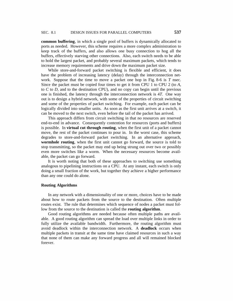
SEC. 8.1 DESIGN ISSUES FOR PARALLEL COMPUTERS 537
common buffering, in which a single pool of buffers is dynamically allocated toports as needed. However, this scheme requires a more complex administration tokeep track of the buffers, and also allows one busy connection to hog all thebuffers, effectively starving other connections. Also, each switch needs to be ableto hold the largest packet, and probably several maximum packets, which tends toincrease memory requirements and drive down the maximum packet size.
While store-and-forward packet switching is flexible and efficient, it doeshave the problem of increasing latency (delay) through the interconnection net-work. Suppose that the time to move a packet one hop in Fig. 8-6 is T nsec.Since the packet must be copied four times to get it from CPU 1 to CPU 2 (to A,to C to D, and to the destination CPU), and no copy can begin until the previousone is finished, the latency through the interconnection network is 4T. One wayout is to design a hybrid network, with some of the properties of circuit switchingand some of the properties of packet switching. For example, each packet can belogically divided into smaller units. As soon as the first unit arrives at a switch, itcan be moved to the next switch, even before the tail of the packet has arrived.
This approach differs from circuit switching in that no resources are reservedend-to-end in advance. Consequently contention for resources (ports and buffers)is possible. In virtual cut through routing, when the first unit of a packet cannotmove, the rest of the packet continues to pour in. In the worst case, this schemedegrades to store-and-forward packet switching. In an alternative approach,wormhole routing, when the first unit cannot go forward, the source is told tostop transmitting, so the packet may end up being strung out over two or possiblyeven more switches like a worm. When the necessary resources become avail-able, the packet can go forward.
It is worth noting that both of these approaches to switching use somethinganalogous to pipelining instructions on a CPU. At any instant, each switch is onlydoing a small fraction of the work, but together they achieve a higher performancethan any one could do alone.
Routing Algorithms
In any network with a dimensionality of one or more, choices have to be madeabout how to route packets from the source to the destination. Often multipleroutes exist. The rule that determines which sequence of nodes a packet must fol-low from the source to the destination is called the routing algorithm.
Good routing algorithms are needed because often multiple paths are avail-able. A good routing algorithm can spread the load over multiple links in order tofully utilize the available bandwidth. Furthermore, the routing algorithm mustavoid deadlock within the interconnection network. A deadlock occurs whenmultiple packets in transit at the same time have claimed resources in such a waythat none of them can make any forward progress and all will remained blockedforever.
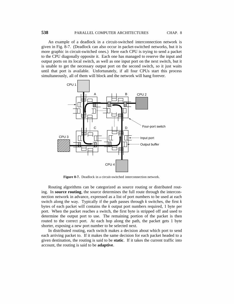
538 PARALLEL COMPUTER ARCHITECTURES CHAP. 8
An example of a deadlock in a circuit-switched interconnection network isgiven in Fig. 8-7. (Deadlock can also occur in packet-switched networks, but it ismore graphic in circuit-switched ones.) Here each CPU is trying to send a packetto the CPU diagonally opposite it. Each one has managed to reserve the input andoutput ports on its local switch, as well as one input port on the next switch, but itis unable to get the necessary output port on the second switch, so it just waitsuntil that port is available. Unfortunately, if all four CPUs start this processsimultaneously, all of them will block and the network will hang forever.
CPU 1
CPU 2
CPU 3
A
C
B
D
Input port
Output buffer
Four-port switch
CPU 4����������
Figure 8-7. Deadlock in a circuit-switched interconnection network.
Routing algorithms can be categorized as source routing or distributed rout-ing. In source routing, the source determines the full route through the intercon-nection network in advance, expressed as a list of port numbers to be used at eachswitch along the way. Typically if the path passes through k switches, the first kbytes of each packet will contains the k output port numbers required, 1 byte perport. When the packet reaches a switch, the first byte is stripped off and used todetermine the output port to use. The remaining portion of the packet is thenrouted to the correct port. At each hop along the path, the packet gets 1 byteshorter, exposing a new port number to be selected next.
In distributed routing, each switch makes a decision about which port to sendeach arriving packet to. If it makes the same decision for each packet headed to agiven destination, the routing is said to be static. If it takes the current traffic intoaccount, the routing is said to be adaptive.

SEC. 8.1 DESIGN ISSUES FOR PARALLEL COMPUTERS 539
One popular routing algorithm for rectangular grids in any number of dimen-sions that is known to be deadlock free is dimensional routing. In this algorithm,the packet is first moved along the x-axis to the correct coordinate, then along they-axis to the correct coordinate, and so on for higher dimensions. For example, togo from (3, 7, 5) to (6, 9, 8), the packet would first go from x = 3 to x = 6 through(4, 7, 5), (5, 7, 5), and (6, 7, 5). Then it would work on the y-axis by going to(6, 8, 5) and (6, 9, 5). Finally, it would go along the z-axis to (6, 9, 6), (6, 9, 7)and (6, 9, 8). This algorithm prevents the cycles that cause a deadlock.
8.1.3 Performance
The point of building a parallel computer is to make it go faster than a unipro-cessor machine. If it does not achieve that simple goal, it is not worth having.Furthermore, it should achieve the goal in a cost-effective manner. A machinethat is twice as fast as a uniprocessor at 50 times the cost is not likely to be a bigseller. In this section we will examine some of the performance issues associatedwith parallel computer architectures.
Hardware Metrics
From a hardware perspective, the performance metrics of interest are the CPUand I/O speeds and the performance of the interconnection network. The CPUand I/O speeds are the same as in the uniprocessor case, so the key parameters ofinterest in a parallel system are those associated with the interconnect. There aretwo key items: latency and bandwidth, which we will now look at in turn.
The roundtrip latency is the time it takes for a CPU to send a packet and get areply. If the packet is sent to a memory, then the latency measures the time toread or write a word or block of words. If it is sent to another CPU, it measuresthe interprocessor communication time for packets of that size. Usually, thelatency of interest is for minimal packets, often one word or a small cache line.
The latency is built up from several factors, and is different for circuit-switched, store-and-forward, virtual cut through, and wormhole-routed intercon-nects. For circuit switching, the latency is the sum of the setup time and thetransmission time. To set up a circuit, a probe packet has to be sent out to reservethe resources and then report back. Once that has happened, the data packet hasto be assembled. When it is ready, bits can flow at full speed, so if the total setuptime is Ts , the packet size is p bits, and the bandwidth b bits/sec, the one-waylatency is Ts + p/b. If the circuit is full duplex, then there is no setup time for thereply, so the minimum latency for sending a p bit packet and getting a p bit replyis Ts + 2p /b sec.
For packet switching, it is not necessary to send a probe packet to the destina-tion in advance, but there is still some internal setup time to assemble the packet,Ta . Here the one-way transmission time is Ta + p/b, but this is only the time to

540 PARALLEL COMPUTER ARCHITECTURES CHAP. 8
get the packet into the first switch. There is a finite delay within the switch, sayTd and then the process is repeated to the next switch and so on. The Td delay iscomposed of both processing time and queueing delay, waiting for the output portto become free. If there are n switches, then the total one-way latency isTa + n(p /b + Td) + p/b, where the final term is due to the copy from the lastswitch to the destination.
The one-way latencies for virtual cut through and wormhole routing in thebest case are close to Ta + p/b because there is no probe packet to set up a circuit,and no store-and-forward delay either. Basically, it is the initial setup time toassemble the packet, plus the time to push the bits out the door. In all cases, pro-pagation delay has to be added, but that is usually small.
The other hardware metric is bandwidth. Many parallel programs, especiallyin the natural sciences, move a lot of data around, so the number of bytes/sec thatthe system can move is critical to performance. Several metrics for bandwidthexist. We have seen one of them—bisection bandwidth—already. Another one isthe aggregate bandwidth, which is computed by simply adding up the capacitiesof all the links. This number gives the maximum number of bits that can be intransit at once. Yet another important metric is the average bandwidth out of eachCPU. If each CPU is capable of outputting 1 MB/sec, it does little good that theinterconnect has a bisection bandwidth of 100 GB/sec. Communication will belimited by how much data each CPU can output.
In practice, actually achieving anything even close to the theoretical band-width is very difficult. Many sources of overhead work to reduce the capacity.For example, there is always some per-packet overhead associated with eachpacket: assembling it, building its header, and getting it going. Sending 1024 4-byte packets will never achieve the same bandwidth as sending 1 4096-bytepacket. Unfortunately, for achieving low latencies, using small packets is better,since large ones block the lines and switches too long. Thus there is an inherentconflict between achieving low average latencies and high-bandwidth utilization.For some applications, one is more important than the other and for other applica-tions it is the other way around. It is worth noting, however, that you can alwaysbuy more bandwidth (by putting in more or wider wires), but you cannot buylower latencies. Thus it is generally better to err on the side of making latenciesas short as possible, and worry about bandwidth later.
Software Metrics
Hardware metrics like latency and bandwidth look at what the hardware iscapable of doing. However, users have a different perspective. They want toknow how much faster their programs are going to run on a parallel computer thanon a uniprocessor. For them, the key metric is speedup: how much faster a pro-gram runs on an n-processor system than on a 1-processor system. Typicallythese results are shown in graphs like those of Fig. 8-8. Here we see several

SEC. 8.1 DESIGN ISSUES FOR PARALLEL COMPUTERS 541
different parallel programs run on a multicomputer consisting of 64 Pentium ProCPUs. Each curve shows the speedup of one program with k CPUs as a functionof k. Perfect speedup is indicated by the dotted line, in which using k CPUsmakes the program go k times faster, for any k. Few programs achieve perfectspeedup, but some come close. The N-body problem parallelizes extremely well;awari (an African board game) does reasonably well; but inverting a certain sky-line matrix does not go more than five times faster no matter how many CPUs areavailable. The programs and results are discussed in (Bal et al., 1998).
6050403020100
60
50
40
30
20
10
0
Spe
edup
Linear speedup
N-body problem
Awari
Skyline matrix inversion
Number of CPUs
Figure 8-8. Real programs achieve less than the perfect speedup indicated bythe dotted line.
Part of the reason that perfect speedup is nearly impossible to achieve is thatalmost all programs have some sequential component, often the initializationphase, reading in the data, or collecting the results. Having many CPUs does nothelp here. Suppose that a program runs for T sec on a uniprocessor, with a frac-tion f of this time being sequential code and a fraction (1 − f ) being potentiallyparallelizable, as shown in Fig. 8-9(a). If the latter code can be run on n CPUswith no overhead, its execution time can be reduced from (1 − f )T to (1 − f )T/nat best, as shown in Fig. 8-9(b). This gives a total execution time for the sequen-tial and parallel parts of fT + (1 − f )T/n. The speedup is just the execution timeof the original program, T, divided by this new execution time:
Speedup =1 + (n − 1)f
n33333333333
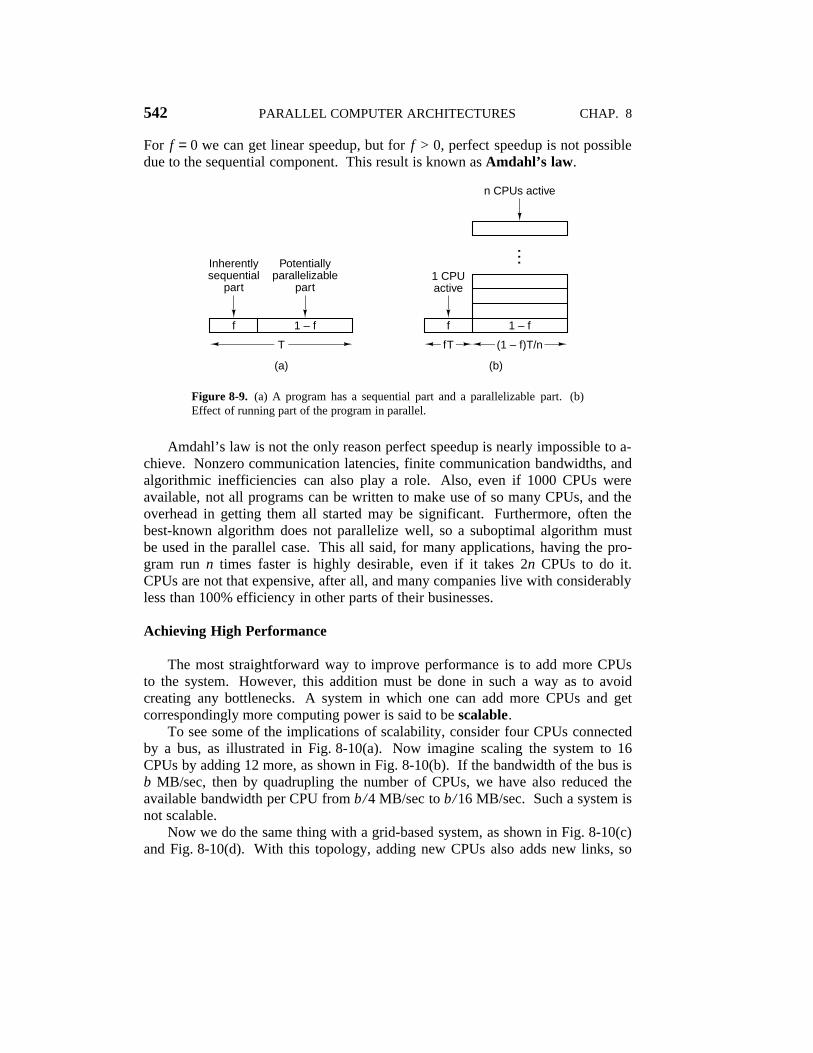
542 PARALLEL COMPUTER ARCHITECTURES CHAP. 8
For f = 0 we can get linear speedup, but for f > 0, perfect speedup is not possibledue to the sequential component. This result is known as Amdahl’s law.
(a)
n CPUs active
1 CPUactive
1 – ff
T
Inherentlysequential
part
(b)
1 – ff
Potentiallyparallelizable
part…
fT (1 – f)T/n
Figure 8-9. (a) A program has a sequential part and a parallelizable part. (b)Effect of running part of the program in parallel.
Amdahl’s law is not the only reason perfect speedup is nearly impossible to a-chieve. Nonzero communication latencies, finite communication bandwidths, andalgorithmic inefficiencies can also play a role. Also, even if 1000 CPUs wereavailable, not all programs can be written to make use of so many CPUs, and theoverhead in getting them all started may be significant. Furthermore, often thebest-known algorithm does not parallelize well, so a suboptimal algorithm mustbe used in the parallel case. This all said, for many applications, having the pro-gram run n times faster is highly desirable, even if it takes 2n CPUs to do it.CPUs are not that expensive, after all, and many companies live with considerablyless than 100% efficiency in other parts of their businesses.
Achieving High Performance
The most straightforward way to improve performance is to add more CPUsto the system. However, this addition must be done in such a way as to avoidcreating any bottlenecks. A system in which one can add more CPUs and getcorrespondingly more computing power is said to be scalable.
To see some of the implications of scalability, consider four CPUs connectedby a bus, as illustrated in Fig. 8-10(a). Now imagine scaling the system to 16CPUs by adding 12 more, as shown in Fig. 8-10(b). If the bandwidth of the bus isb MB/sec, then by quadrupling the number of CPUs, we have also reduced theavailable bandwidth per CPU from b/4 MB/sec to b/16 MB/sec. Such a system isnot scalable.
Now we do the same thing with a grid-based system, as shown in Fig. 8-10(c)and Fig. 8-10(d). With this topology, adding new CPUs also adds new links, so
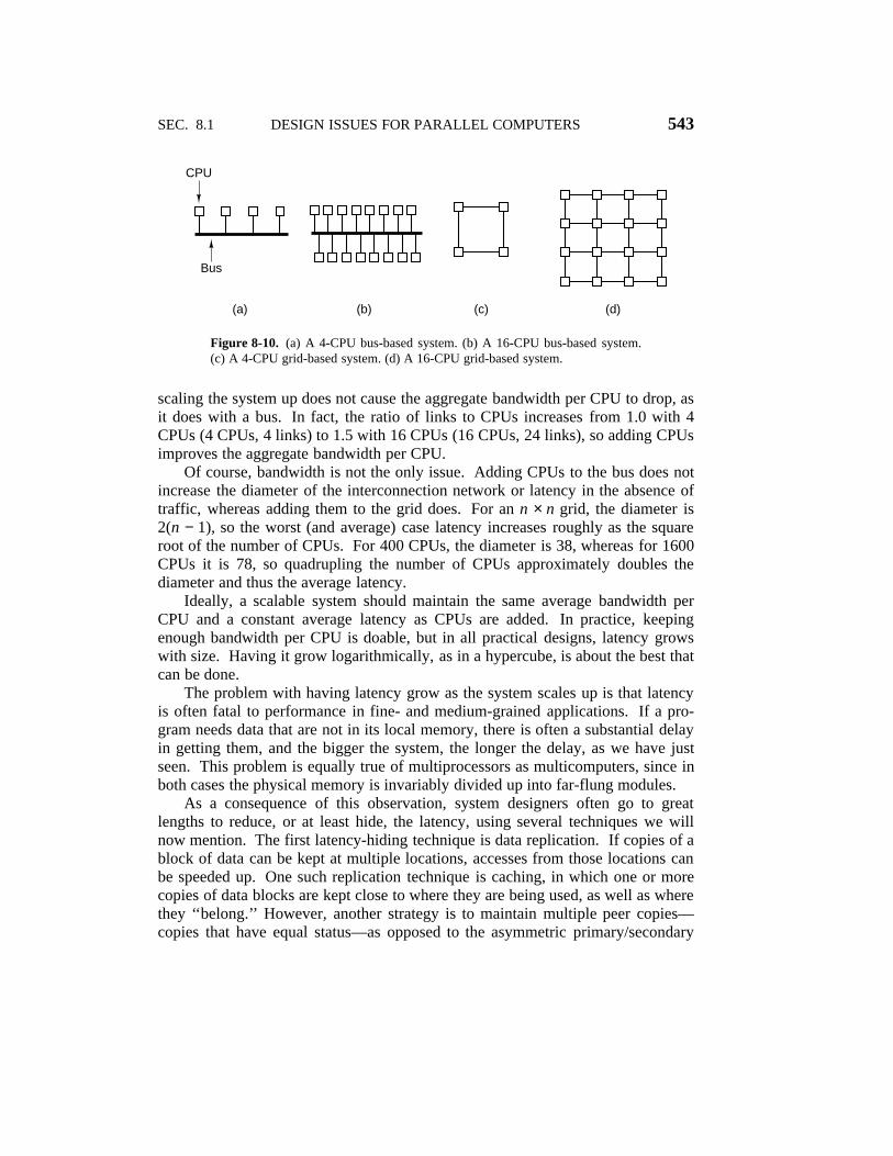
SEC. 8.1 DESIGN ISSUES FOR PARALLEL COMPUTERS 543
CPU
Bus
(a) (b) (c) (d)
Figure 8-10. (a) A 4-CPU bus-based system. (b) A 16-CPU bus-based system.(c) A 4-CPU grid-based system. (d) A 16-CPU grid-based system.
scaling the system up does not cause the aggregate bandwidth per CPU to drop, asit does with a bus. In fact, the ratio of links to CPUs increases from 1.0 with 4CPUs (4 CPUs, 4 links) to 1.5 with 16 CPUs (16 CPUs, 24 links), so adding CPUsimproves the aggregate bandwidth per CPU.
Of course, bandwidth is not the only issue. Adding CPUs to the bus does notincrease the diameter of the interconnection network or latency in the absence oftraffic, whereas adding them to the grid does. For an n × n grid, the diameter is2(n − 1), so the worst (and average) case latency increases roughly as the squareroot of the number of CPUs. For 400 CPUs, the diameter is 38, whereas for 1600CPUs it is 78, so quadrupling the number of CPUs approximately doubles thediameter and thus the average latency.
Ideally, a scalable system should maintain the same average bandwidth perCPU and a constant average latency as CPUs are added. In practice, keepingenough bandwidth per CPU is doable, but in all practical designs, latency growswith size. Having it grow logarithmically, as in a hypercube, is about the best thatcan be done.
The problem with having latency grow as the system scales up is that latencyis often fatal to performance in fine- and medium-grained applications. If a pro-gram needs data that are not in its local memory, there is often a substantial delayin getting them, and the bigger the system, the longer the delay, as we have justseen. This problem is equally true of multiprocessors as multicomputers, since inboth cases the physical memory is invariably divided up into far-flung modules.
As a consequence of this observation, system designers often go to greatlengths to reduce, or at least hide, the latency, using several techniques we willnow mention. The first latency-hiding technique is data replication. If copies of ablock of data can be kept at multiple locations, accesses from those locations canbe speeded up. One such replication technique is caching, in which one or morecopies of data blocks are kept close to where they are being used, as well as wherethey ‘‘belong.’’ However, another strategy is to maintain multiple peer copies—copies that have equal status—as opposed to the asymmetric primary/secondary

544 PARALLEL COMPUTER ARCHITECTURES CHAP. 8
relationship used in caching. When multiple copies are maintained, in whateverform, key issues are where the data blocks are placed, when, and by whom.Answers range from dynamic placement on demand by the hardware, to inten-tional placement at load time following compiler directives. In all cases, manag-ing consistency is an issue.
A second technique for hiding latency is prefetching . If a data item can befetched before it is needed, the fetching process can be overlapped with normalexecution, so that when the item is needed, it will be there. Prefetching can beautomatic or under program control. When a cache loads not only the word beingreferenced, but an entire cache line containing the word, it is gambling that thesucceeding words are also likely to be needed soon.
Prefetching can also be controlled explicitly. When the compiler realizes thatit will need some data, it can put in an explicit instruction to go get them, and putthat instruction sufficiently far in advance that the data will be there in time. Thisstrategy requires that the compiler have a complete knowledge of the underlyingmachine and its timing, as well as control over where all data are placed. Suchspeculative LOAD instructions work best when it is known for sure that the datawill be needed. Getting a page fault on a LOAD for a path that is ultimately nottaken is very costly.
A third technique that can hide latency is multithreading. Most modern sys-tems support the concept of multiprogramming, in which multiple processes canrun simultaneously (or in pseudoparallel on a timesharing basis). If switchingbetween processes can be made fast enough, for example, by giving each one itsown memory map and hardware registers, then when one process blocks waitingfor remote data to arrive, the hardware can quickly switch to another one that isable to continue. In the limiting case, the CPU runs the first instruction fromthread one, the second instruction from thread two, and so on. In this way, theCPU can be kept busy, even in the face of long memory latencies for the indivi-dual threads.
In fact, some machines automatically cycle among the processes, switchingafter every instruction, to hide long latencies. One of the first supercomputers, theCDC 6600, carried this idea to such an extreme that it was advertised as having 10peripheral processing units that could run in parallel. In reality there was only oneperipheral processor, which simulated 10 of them by running instructions fromeach one in round robin order, first one instruction from peripheral processor 1,then one instruction from peripheral processor 2, and so on.
A fourth technique for hiding latency is using nonblocking writes. Normally,when a STORE instruction is executed, the CPU waits until the STORE has com-pleted before continuing. With nonblocking writes, the memory operation isstarted, but the program just continues anyway. Continuing past a LOAD is harder,but with out-of-order execution, even that is possible.

SEC. 8.1 DESIGN ISSUES FOR PARALLEL COMPUTERS 545
8.1.4 Software
Although this chapter is primarily about parallel computer architectures, a fewwords about software are appropriate too. After all, without parallel software,parallel hardware is of little use, so good hardware designers take the needs of thesoftware into account when designing the hardware. For a discussion aboutsoftware for parallel computers, see (Wilkinson and Allen, 1999).
There are four general approaches to producing software for parallel comput-ers. At one extreme is the addition of special numerical libraries to otherwise nor-mal sequential languages. For example, a library procedure to invert a largematrix or solve a set of partial differential equations could be called from asequential program and do its work on a parallel processor without the program-mer even being aware of the existence of parallelism. The trouble with thisapproach is that parallelism can only be used in a few procedures and the bulk ofthe code will remain sequential.
A second approach is the addition of special libraries containing communica-tion and control primitives. Here the programmer is responsible for creating andmanaging the parallelism within a conventional programming language usingthese additional primitives.
The next step up is to add a few special constructs to existing programminglanguages, such as the ability to fork off new parallel processes easily, execute theiterations of a loop in parallel, or do arithmetic on all the elements of a vector atthe same time. This approach is widely used and numerous programming lang-uages have been modified to include some parallelism.
The most extreme approach is to invent an entirely new language especiallyfor parallel processing. The obvious advantage of inventing a new language isthat such a language is well suited for parallel programming, but the equally obvi-ous disadvantage is that programmers must learn a new language. Quite a few ofthem have something else to do with their time. Most new parallel languages areimperative (with instructions to modify state variables), but a few are functional,logic based, or object oriented.
There have been so many libraries, extensions, and new languages inventedfor parallel programming, and they span such a broad spectrum of possibilities,that it is impossible to classify all of them in any reasonable way. Instead of eventrying, we will focus on five key issues that form the heart of all software forparallel computers:
1. Control models.
2. Granularity of parallelism.
3. Computational paradigms.
4. Communication methods.
5. Synchronization primitives.

546 PARALLEL COMPUTER ARCHITECTURES CHAP. 8
Each of these will now be discussed in turn.
Control Models
Probably the most fundamental choice the software must make is whetherthere will be one thread of control or multiple threads of control. In the formermodel, there is one program and one program counter, but multiple sets of data.As each instruction is issued, it is carried out on all data sets simultaneously, bydifferent processing elements.
As an example, imagine a weather program with hourly temperature measure-ments from thousands of remote sensors that have to be averaged for each sensor.When the program issues the instruction
LOAD THE TEMPERATURE FOR 1 A.M. INTO REGISTER R1
each processor carries it out, using its own data and its own R1. Later, when theprogram issues the instruction
ADD THE TEMPERATURE FOR 2 A.M. TO REGISTER R1
again, each processor does it using its own data. At the end of the calculation,each processor will have computed the mean temperature for a different sensor.
The implications for this programming model for the hardware are enormous.It effectively says that each processing element is basically an ALU and amemory, with no instruction decoding logic of its own. Instead a single central-ized unit fetches instructions and tells the ALUs what to do next.
In the alternative model, multiple threads of control exist, each one with itsown program counter, registers, and local variables. Each thread of control exe-cutes its own program on its own data, possibly communicating or synchronizingwith other threads of control from time to time. Many variations on this basicidea exist, and together they form the dominant model for parallel processing. Forthis reason, we will now focus primarily on parallel computing involving multiplethreads of control.
Granularity of Parallelism
Control parallelism can be introduced at various levels. At the lowest level,individual machine instructions can contain parallelism (e.g., the IA-64). At thislevel, programmers are usually not aware of the parallelism; it is managed by thecompiler or hardware.
One level up we come to block-level parallelism, which allows programmersexplicit control over which statements are to be executed sequentially and whichin parallel. One of the most elegant ways of expressing this kind of parallelism isdue to Algol 68, in which
SEC. 8.1 DESIGN ISSUES FOR PARALLEL COMPUTERS 547
begin Statement-1; Statement-2; Statement-3 end
was used to create a block with (for example) three arbitrary statements to be exe-cuted sequentially. In contrast,
begin Statement-1, Statement-2, Statement-3 end
was used to execute the same three statements in parallel. By careful placementof semicolons, commas, parentheses, and begin/end delimiters, arbitrary combi-nations of sequential and parallel execution could be expressed.
A somewhat coarser grain of parallelism is present when it is possible to call aprocedure and not have the caller wait for it before continuing. Not waitingmeans that the caller and callee will run in parallel. If the caller is in a loop thatcalls a procedure on every iteration and waits for none of them, then a largenumber of parallel procedures can be started at once.
Another form of parallelism is to have a method for a process to create or forkoff multiple threads or lightweight processes, all of which run within the processaddress space. Each thread has its own program counter, registers, and stack butotherwise shares all the rest of the address space (and all the global variables)with all the other threads. (In contrast to threads, different processes do not sharea common address space.) Threads run independently of one another, possibly ondifferent CPUs. In some systems, the operating system is aware of all the threadsand does the thread scheduling. In other systems, each user process does its ownthread scheduling and management, without the operating system even knowingabout the threads.
Finally, the coarsest form of parallelism is having multiple independentprocesses work together to solve a problem. Unlike threads, which share a com-mon address space, independent processes do not, so they must cooperate at arms’length, which means that the problem must be divided into relatively largechunks, one for each process. However, independent processes also offer themost opportunity for exploiting large-scale parallelism especially on multicomput-ers.
Computational Paradigms
Most parallel programs, especially those involving large numbers of threadsor independent processes, use some underlying paradigm to structure their work.Many such paradigms exist. In this section we will just mention a few of themore popular ones.
A generalization of the idea of having a parallel program consist of one threadof control and multiple execution units is the SPMD (Single Program MultipleData) paradigm. The idea here is that although the system consists of multipleindependent processes, they all run the same program, but on different data sets.Only now, unlike in the temperature example, they are not in lockstep, synchron-ized down to the last instruction. Instead, each one performs the same

548 PARALLEL COMPUTER ARCHITECTURES CHAP. 8
computation, but at its own pace.A second paradigm is the pipeline, illustrated in Fig. 8-11(a) with three
processes. Data are fed into the first process, which transforms them and outputsthem for the second process to read, and so on. If the data stream is long (e.g., avideo presentation), all the processors may be busy at the same time. UNIX pipe-lines work like this and can be run as separate processes in parallel on a multi-computer or multiprocessor.
Process
P1
(d)
P2
P5 P6
P3
P2P1 P3
P8P7
P1
P9
P1
P2
P3
P2 P3
Synchronization point
P1 P2 P3
Synchronization point
P4
Work queue
(c)(b)(a)
Figure 8-11. Computational paradigms. (a) Pipeline. (b) Phased computation.(c) Divide and conquer. (d) Replicated worker.
Another paradigm is the computation of Fig. 8-11(b), in which the work isdivided up into phases, for example, iterations of a loop. During each phase, mul-tiple processes work in parallel, but when each one has finished, it waits until allthe others are done too before starting the next phase. A fourth paradigm isdivide and conquer, depicted in Fig. 8-11(c), in which one process starts off andthen forks off other processes to which it can pass some of the work. An analogyin the construction world is a general contractor who gets an order, then subcon-tracts out much of the work to masonry, electrical, plumbing, painting, and othersubcontractors. These, in turn, may contract out some of their work to yet morespecialized subcontractors.
Our last model is the replicated worker paradigm, sometimes called a taskfarm, and illustrated in Fig. 8-11(d). Here, a centralized work queue exists andworkers take tasks out of the queue and complete them. If a task generates newtasks, these are added to the central queue. Whenever a worker finishes itscurrent task, it goes to the task queue to get a new one. This paradigm can also beimplemented with an active manager at the top handing out work, rather than
SEC. 8.1 DESIGN ISSUES FOR PARALLEL COMPUTERS 549
having the workers forage for it on their own.
Communication Methods
When a program is split up into pieces, say, processes, which run in parallel,the pieces (processes) often need to communicate with one another. This com-munication can be done in one of two ways: shared variables or explicit messagepassing. In the former method, all the processes have access to the common logi-cal memory and can communicate by reading and writing it. For example, oneprocess can set a variable and another one, in a different process, can read it.
On a multiprocessor, variables can be shared among multiple processes bymapping the same page into each process’ address space. Then shared variablescan be read and written using ordinary LOAD and STORE machine instructions.However, even on a multicomputer, with no shared physical memory, logicalsharing of variables is still possible, albeit slightly more complicated. As we sawabove, Linda supports the notation of a shared tuple space, even on a multicom-puter, and Orca supports the concept of shared objects across machine boundaries.Sharing a single address space on a multicomputer and paging over the intercon-nection network is also a possibility. In short, allowing processes to communicatethrough shared variables is possible on both multiprocessors and multicomputers.
The alternative to communication via shared memory is communication viaexplicit message passing. In this model, processes use primitives such as send andreceive to communicate. One process does a send, naming another process as thedestination. As soon as the latter does a receive, the message is copied into thereceiver’s address space.
Message passing has many variations, but all of them come down to havingtwo primitives send and receive which are used to transmit messages. These aregenerally implemented as system calls. We will go into some of the details laterin this chapter.
Another issue in message passing is how many receivers there are. The sim-plest case is one sender and one receiver, known as point-to-point message pass-ing. However, sometimes it is useful for a message to be delivered to allprocesses, called broadcasting, or to a specific subset of the processes, known asmulticasting.
It should be noted that message passing is easy to implement on a multipro-cessor by simply copying from the sender to the receiver. Thus the issues of phy-sical shared memory (multiprocessor versus multicomputer) and logical sharedmemory (communication via shared variables versus explicit message passing)are separate. All four combinations make sense and can be implemented. Theyare listed in Fig. 8-12.
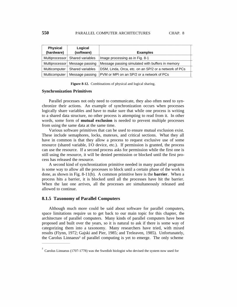
550 PARALLEL COMPUTER ARCHITECTURES CHAP. 8
22222222222222222222222222222222222222222222222222222222222222222222222222222222222222Physical
(hardware)Logical
(software) Examples22222222222222222222222222222222222222222222222222222222222222222222222222222222222222Multiprocessor Shared variables Image processing as in Fig. 8-122222222222222222222222222222222222222222222222222222222222222222222222222222222222222Multiprocessor Message passing Message passing simulated with buffers in memory22222222222222222222222222222222222222222222222222222222222222222222222222222222222222Multicomputer Shared variables DSM, Linda, Orca, etc. on an SP/2 or a network of PCs22222222222222222222222222222222222222222222222222222222222222222222222222222222222222Multicomputer Message passing PVM or MPI on an SP/2 or a network of PCs2222222222222222222222222222222222222222222222222222222222222222222222222222222222222211
11111111
1111111111
1111111111
1111111111
Figure 8-12. Combinations of physical and logical sharing.
Synchronization Primitives
Parallel processes not only need to communicate, they also often need to syn-chronize their actions. An example of synchronization occurs when processeslogically share variables and have to make sure that while one process is writingto a shared data structure, no other process is attempting to read from it. In otherwords, some form of mutual exclusion is needed to prevent multiple processesfrom using the same data at the same time.
Various software primitives that can be used to ensure mutual exclusion exist.These include semaphores, locks, mutexes, and critical sections. What they allhave in common is that they allow a process to request exclusive use of someresource (shared variable, I/O device, etc.). If permission is granted, the processcan use the resource. If a second process asks for permission while the first one isstill using the resource, it will be denied permission or blocked until the first pro-cess has released the resource.
A second kind of synchronization primitive needed in many parallel programsis some way to allow all the processes to block until a certain phase of the work isdone, as shown in Fig. 8-11(b). A common primitive here is the barrier. When aprocess hits a barrier, it is blocked until all the processes have hit the barrier.When the last one arrives, all the processes are simultaneously released andallowed to continue.
8.1.5 Taxonomy of Parallel Computers
Although much more could be said about software for parallel computers,space limitations require us to get back to our main topic for this chapter, thearchitecture of parallel computers. Many kinds of parallel computers have beenproposed and built over the years, so it is natural to ask if there is some way ofcategorizing them into a taxonomy. Many researchers have tried, with mixedresults (Flynn, 1972; Gajski and Pier, 1985; and Treleaven, 1985). Unfortunately,the Carolus Linnaeus† of parallel computing is yet to emerge. The only scheme3333333333333333
† Carolus Linnaeus (1707-1778) was the Swedish biologist who devised the system now used for

SEC. 8.1 DESIGN ISSUES FOR PARALLEL COMPUTERS 551
that is used much is Flynn’s, and even his is, at best, a very crude approximation.It is given in Fig. 8-13.
2222222222222222222222222222222222222222222222222222222222222222222222222Instructionstreams
Datastreams Name Examples2222222222222222222222222222222222222222222222222222222222222222222222222
1 1 SISD Classical Von Neumann machine22222222222222222222222222222222222222222222222222222222222222222222222221 Multiple SIMD Vector supercomputer, array processor2222222222222222222222222222222222222222222222222222222222222222222222222Multiple 1 MISD Arguably none2222222222222222222222222222222222222222222222222222222222222222222222222Multiple Multiple MIMD Multiprocessor, multicomputer22222222222222222222222222222222222222222222222222222222222222222222222221111111111
1111111111
1111111111
1111111111
1111111111
Figure 8-13. Flynn’s taxonomy of parallel computers.
Flynn’s classification is based on two concepts—instruction streams and datastreams. An instruction stream corresponds to a program counter. A system withn CPUs has n program counters, hence n instruction streams.
A data stream consists of a set of operands. The temperature computationexample given earlier has multiple data streams, one for each sensor.
The instruction and data streams are, to some extent, independent, so fourcombinations exist, as listed in Fig. 8-13. SISD is just the classical, sequentialvon Neumann computer. It has one instruction stream, one data stream, and doesone thing at a time. SIMD machines have a single control unit that issues oneinstruction at a time, but they have multiple ALUs to carry it out on multiple datasets simultaneously. The ILLIAC IV (Fig. 2-8) is the prototype of SIMDmachines. Modern SIMD machines exist and are used for scientific computing.
MISD machines are a somewhat strange category, with multiple instructionsoperating on the same piece of data. It is not clear if any such machines exist,although some people regard pipelined machines as MISD.
Finally, we have MIMD, which are just multiple independent CPUs operatingas part of a larger system. Most parallel processors fall into this category. Bothmultiprocessors and multicomputers are MIMD machines.
Flynn’s taxonomy stops here, but we have extended it in Fig. 8-14. SIMD hasbeen split into two subgroups. The first one is for numeric supercomputers andother machines that operate on vectors, performing the same operation on eachvector element. The second one is for parallel-type machines, such as theILLIAC IV, in which a master control unit broadcasts instructions to manyindependent ALUs.
In our taxonomy, the MIMD category has been split into multiprocessors(shared-memory machines), and multicomputers (message-passing machines).Three kinds of multiprocessors exist, distinguished by the way the shared memoryis implemented on them. They are called UMA (Uniform Memory Access),NUMA (NonUniform Memory Access), and COMA (Cache Only Memory3333333333333333classifying all plants and animals into kingdom, phylum, class, order, family, genus, and species.

552 PARALLEL COMPUTER ARCHITECTURES CHAP. 8
SISD
(Von Neumann)
SIMD
Parallel computer architectures
MISD
?
MIMD
Vectorprocessor
Arrayprocessor
Multi-processors
Multi-computers
UMA COMA NUMA MPP COW
Bus Switched CC-NUMA NC-NUMA GridHyper-cube
Shared memory Message passing
Figure 8-14. A taxonomy of parallel computers.
Access). These categories exist because in large multiprocessors, the memory isusually split up into multiple modules. UMA machines have the property thateach CPU has the same access time to every memory module. In other words,every memory word can be read as fast as every other memory word. If this istechnically impossible, the fastest references are slowed down to match theslowest ones, so programmers do not see the difference. This is what ‘‘uniform’’means here. This uniformity makes the performance predictable, an importantfactor for writing efficient code.
In contrast, in a NUMA multiprocessor, this property does not hold. Oftenthere is a memory module close to each CPU and accessing that memory moduleis much faster than accessing distant ones. The result is that for performance rea-sons, it matters where code and data are placed. COMA machines are also nonun-iform, but in a different way. We will study each of these types and their sub-categories in detail later.
The other main category of MIMD machines consists of the multicomputers,which, unlike the multiprocessors, do not have shared primary memory at thearchitectural level. In other words, the operating system on a multicomputer CPUcannot access memory attached to a different CPU by just executing a LOADinstruction. It has to send an explicit message and wait for an answer. The abilityof the operating system to read a distant word by just doing a LOAD is what

SEC. 8.1 DESIGN ISSUES FOR PARALLEL COMPUTERS 553
distinguishes multiprocessors from multicomputers. As we mentioned before,even on a multicomputer, user programs may have the ability to access remotememory by using LOAD and STORE instructions, but this illusion is supported bythe operating system, not the hardware. This difference is subtle, but very impor-tant. Because multicomputers do not have direct access to remote memory, theyare sometimes called NORMA (NO Remote Memory Access) machines.
Multicomputers can be roughly divided into two categories. The firstcategory contains the MPPs (Massively Parallel Processors), which are expen-sive supercomputers consisting of many CPUs tightly coupled by a high-speedproprietary interconnection network. The Cray T3E and IBM SP/2 are well-known examples.
The other category consists of regular PCs or workstations, possibly rack-mounted, and connected by commercial off-the-shelf interconnection technology.Logically, there is not much difference, but huge supercomputers costing manymillions of dollars are used differently than networks of PCs assembled by theusers for a fraction of the price of an MPP. These home-brew machines go byvarious names, including NOW (Network of Workstations) and COW (Clusterof Workstations).
In the following sections, we will look at the main categories, SIMD,MIMD/multiprocessors, and MIMD/multicomputers in some detail. The goal isto give a good overview of what each type is like, what the subcategories are, andwhat the key design principles are. Several examples will be used for illustration.

ABINARY NUMBERS
1
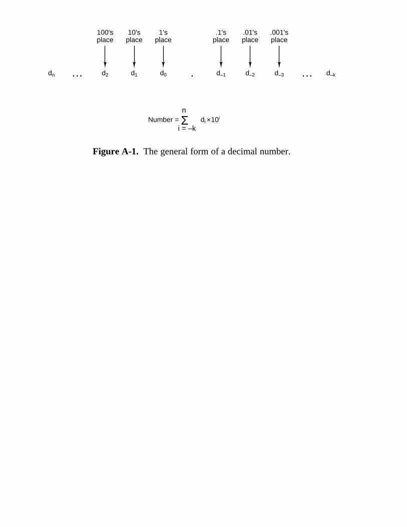
100'splace
10'splace
1'splace
.1'splace
.01'splace
.001'splace
dn d2 d1 d0 d–1 d–2 d–3 d–k
Number = n
i = –kdi 10i
… ….
× Σ
Figure A-1. The general form of a decimal number.
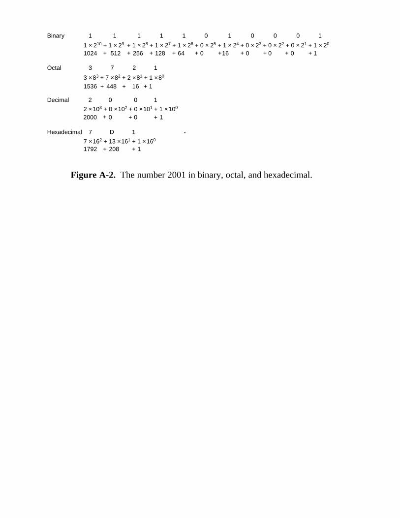
.
Binary
Octal
Decimal
Hexadecimal
1 1 1 1 1 1 10 0 00
7 1D
1 × 210 + 1 × 29 + 1 × 28 + 1 × 27 + 1 × 26 + 0 × 25 + 1 × 24 + 0 × 23 + 0 × 22 + 0 × 21 + 1 × 20
3 7 2 1
3 × 83 + 7 × 82 + 2 × 81 + 1 × 80
2 0 0 1
2 × 10³ + 0 × 102 + 0 × 101 + 1 × 100
++ +
7 × 162 + 13 × 161 + 1 × 160
1792 1208+ +
10 0 016 0
116
64128256 512+ + + +
+++
+ + + + + +1024
4481536
2000 100
Figure A-2. The number 2001 in binary, octal, and hexadecimal.

2222222222222222222222222222222222222222Decimal Binary Octal Hex2222222222222222222222222222222222222222
0 0 0 022222222222222222222222222222222222222221 1 1 122222222222222222222222222222222222222222 10 2 222222222222222222222222222222222222222223 11 3 322222222222222222222222222222222222222224 100 3 322222222222222222222222222222222222222225 101 5 522222222222222222222222222222222222222226 110 6 622222222222222222222222222222222222222227 111 7 722222222222222222222222222222222222222228 1000 10 822222222222222222222222222222222222222229 1001 11 92222222222222222222222222222222222222222
10 1010 12 A222222222222222222222222222222222222222211 1011 13 B222222222222222222222222222222222222222212 1100 14 C222222222222222222222222222222222222222213 1101 15 D222222222222222222222222222222222222222214 1110 16 E222222222222222222222222222222222222222215 1111 17 F222222222222222222222222222222222222222216 10000 20 10222222222222222222222222222222222222222220 10100 24 14222222222222222222222222222222222222222230 11110 36 1E222222222222222222222222222222222222222240 101000 50 28222222222222222222222222222222222222222250 110010 62 32222222222222222222222222222222222222222260 111100 74 3C222222222222222222222222222222222222222270 1000110 106 46222222222222222222222222222222222222222280 1010000 120 50222222222222222222222222222222222222222290 1011010 132 5A2222222222222222222222222222222222222222
100 11001000 144 6422222222222222222222222222222222222222221000 1111101000 1750 3E822222222222222222222222222222222222222222989 101110101101 5655 BA222222222222222222222222222222222222222211
111111111111111111111111111111111111
11111111111111111111111111111111111111
11111111111111111111111111111111111111
11111111111111111111111111111111111111
11111111111111111111111111111111111111
Figure A-3. Decimal numbers and their binary, octal, and hex-adecimal equivalents.

Example 1
Hexadecimal
Binary
Octal
Hexadecimal
Binary
Octal
Example 2
1
1
9 4
4
4
8 B
B
6
1
4
4
5
5
0
0
7
7 7
AB C
5 5
56
4
3
3
0 0 0 1 1 0 0 1 0 1 0 0 1 0 0 0 1 0 1 1 0 1 1 0 0
0 1 1 1 1 0 1 1 1 0 1 0 0 0 1 1 1 0 1 1 1 1 0 0 0 1 0 0
.
.
.
.
.
.
Figure A-4. Examples of octal-to-binary and hexadecimal-to-binary conversion.

Quotients Remainders
1 4 9 2
7 4 6
3 7 3
1 8 6
9 3
4 6
2 3
1 1
5
2
1
0
1
0
0
0
1
1
1
1
1
0
0
1 0 1 1 1 0 1 0 1 0 0 = 149210
Figure A-5. Conversion of the decimal number 1492 to binaryby successive halving, starting at the top and working down-ward. For example, 93 divided by 2 yields a quotient of 46 anda remainder of 1, written on the line below it.
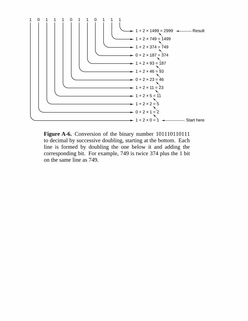
1 + 2 × 1499 = 2999
01 1 1 1 0 1 1 0 1 1 1
Result
1 + 2 × 749 = 1499
1 + 2 × 374 = 749
0 + 2 × 187 = 374
1 + 2 × 93 = 187
1 + 2 × 46 = 93
0 + 2 × 23 = 46
1 + 2 × 11 = 23
1 + 2 × 5 = 11
1 + 2 × 2 = 5
0 + 2 × 1 = 2
1 + 2 × 0 = 1 Start here
Figure A-6. Conversion of the binary number 101110110111to decimal by successive doubling, starting at the bottom. Eachline is formed by doubling the one below it and adding thecorresponding bit. For example, 749 is twice 374 plus the 1 biton the same line as 749.
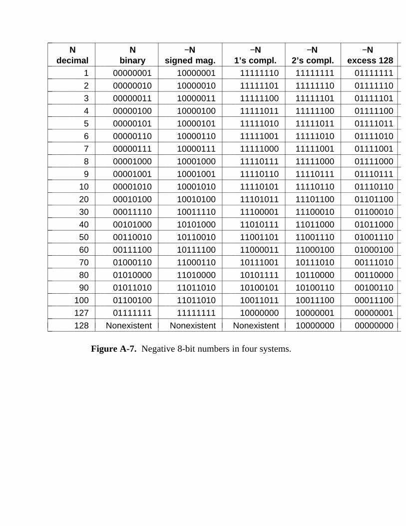
2222222222222222222222222222222222222222222222222222222222222222222222222222222222N
decimalN
binary−N
signed mag.−N
1’s compl.−N
2’s compl.−N
excess 12822222222222222222222222222222222222222222222222222222222222222222222222222222222221 00000001 10000001 11111110 11111111 0111111122222222222222222222222222222222222222222222222222222222222222222222222222222222222 00000010 10000010 11111101 11111110 0111111022222222222222222222222222222222222222222222222222222222222222222222222222222222223 00000011 10000011 11111100 11111101 0111110122222222222222222222222222222222222222222222222222222222222222222222222222222222224 00000100 10000100 11111011 11111100 0111110022222222222222222222222222222222222222222222222222222222222222222222222222222222225 00000101 10000101 11111010 11111011 0111101122222222222222222222222222222222222222222222222222222222222222222222222222222222226 00000110 10000110 11111001 11111010 0111101022222222222222222222222222222222222222222222222222222222222222222222222222222222227 00000111 10000111 11111000 11111001 0111100122222222222222222222222222222222222222222222222222222222222222222222222222222222228 00001000 10001000 11110111 11111000 0111100022222222222222222222222222222222222222222222222222222222222222222222222222222222229 00001001 10001001 11110110 11110111 011101112222222222222222222222222222222222222222222222222222222222222222222222222222222222
10 00001010 10001010 11110101 11110110 01110110222222222222222222222222222222222222222222222222222222222222222222222222222222222220 00010100 10010100 11101011 11101100 01101100222222222222222222222222222222222222222222222222222222222222222222222222222222222230 00011110 10011110 11100001 11100010 01100010222222222222222222222222222222222222222222222222222222222222222222222222222222222240 00101000 10101000 11010111 11011000 01011000222222222222222222222222222222222222222222222222222222222222222222222222222222222250 00110010 10110010 11001101 11001110 01001110222222222222222222222222222222222222222222222222222222222222222222222222222222222260 00111100 10111100 11000011 11000100 01000100222222222222222222222222222222222222222222222222222222222222222222222222222222222270 01000110 11000110 10111001 10111010 00111010222222222222222222222222222222222222222222222222222222222222222222222222222222222280 01010000 11010000 10101111 10110000 00110000222222222222222222222222222222222222222222222222222222222222222222222222222222222290 01011010 11011010 10100101 10100110 001001102222222222222222222222222222222222222222222222222222222222222222222222222222222222
100 01100100 11011010 10011011 10011100 000111002222222222222222222222222222222222222222222222222222222222222222222222222222222222127 01111111 11111111 10000000 10000001 000000012222222222222222222222222222222222222222222222222222222222222222222222222222222222128 Nonexistent Nonexistent Nonexistent 10000000 00000000222222222222222222222222222222222222222222222222222222222222222222222222222222222211
11111111111111111111111111111111
1111111111111111111111111111111111
1111111111111111111111111111111111
1111111111111111111111111111111111
1111111111111111111111111111111111
1111111111111111111111111111111111
1111111111111111111111111111111111
Figure A-7. Negative 8-bit numbers in four systems.

Addend 0 0 1 1Augend +033 +133 +033 +133Sum 0 1 1 0Carry 0 0 0 1
Figure A-8. The addition table in binary.

Decimal 1's complement 2's complement
10+ (−3)
+7
0000101011111100
1 00000110
carry 1
00000111
0000101011111101
1 00000111
discarded
Figure A-9. Addition in one’s complement and two’s complement.

BFLOATING-POINT NUMBERS
1

1Negativeoverflow
2Expressible
negative numbers
3Negativeunderflow
4Zero
5Positive
underflow6
Expressiblepositive numbers
7Positiveoverflow
—10100 —10—100 0 1010010—100
Figure B-1. The real number line can be divided into seven regions.

2222222222222222222222222222222222222222222222222222222222222222Digits in fraction Digits in exponent Lower bound Upper bound2222222222222222222222222222222222222222222222222222222222222222
3 1 10−12 1092222222222222222222222222222222222222222222222222222222222222222
3 2 10−102 10992222222222222222222222222222222222222222222222222222222222222222
3 3 10−1002 109992222222222222222222222222222222222222222222222222222222222222222
3 4 10−10002 1099992222222222222222222222222222222222222222222222222222222222222222
4 1 10−13 1092222222222222222222222222222222222222222222222222222222222222222
4 2 10−103 10992222222222222222222222222222222222222222222222222222222222222222
4 3 10−1003 109992222222222222222222222222222222222222222222222222222222222222222
4 4 10−10003 1099992222222222222222222222222222222222222222222222222222222222222222
5 1 10−14 1092222222222222222222222222222222222222222222222222222222222222222
5 2 10−104 10992222222222222222222222222222222222222222222222222222222222222222
5 3 10−1004 109992222222222222222222222222222222222222222222222222222222222222222
5 4 10−10004 1099992222222222222222222222222222222222222222222222222222222222222222
10 3 10−1009 109992222222222222222222222222222222222222222222222222222222222222222
20 3 10−1019 109992222222222222222222222222222222222222222222222222222222222222222111111111111111111111111111
111111111111111111111111111
111111111111111111111111111
111111111111111111111111111
111111111111111111111111111
Figure B-2. The approximate lower and upper bounds of ex-pressible (unnormalized) floating-point decimal numbers.
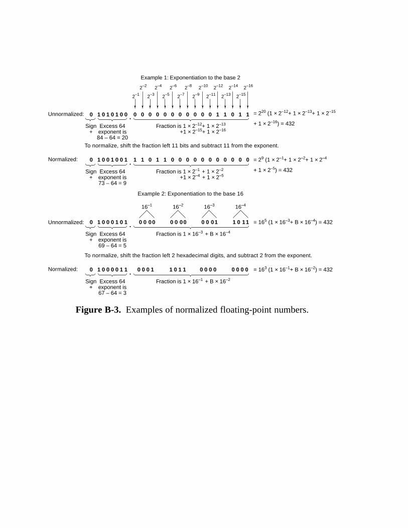
2–1
2–2
Unnormalized:
Sign+
Excess 64exponent is84 – 64 = 20
Fraction is 1 × 2–12+ 1 × 2–13
+1 × 2–15+ 1 × 2–16
Normalized:
Example 1: Exponentiation to the base 2
= 220 (1 × 2–12+ 1 × 2–13+ 1 × 2–15
+ 1 × 2–16) = 432
= 29 (1 × 2–1+ 1 × 2–2+ 1 × 2–4
+ 1 × 2–5) = 432
= 165 (1 × 16–3+ B × 16–4) = 432
To normalize, shift the fraction left 11 bits and subtract 11 from the exponent.
Sign+
Excess 64exponent is73 – 64 = 9
Fraction is 1 × 2–1 + 1 × 2–2
+1 × 2–4 + 1 × 2–5
Sign+
Excess 64exponent is69 – 64 = 5
Fraction is 1 × 16–3 + B × 16–4
2–3
2–4
2–5
2–6
2–7
2–8
2–9
2–10
2–11
2–12
2–13
2–14
2–15
2–16
00 0 0 0 0 0 0 0 0 0 0 1 1 01 1 10 0 0 0 1 1
10 1 0 1 1 0 0 0 0 0 0 0 0 01 0 00 1 0 1 0 0
Normalized: = 163 (1 × 16–1+ B × 16–2) = 432
To normalize, shift the fraction left 2 hexadecimal digits, and subtract 2 from the exponent.
Sign+
Excess 64exponent is67 – 64 = 3
Fraction is 1 × 16–1 + B × 16–2
00 0 0 1 1 0 1 1 0 0 0 0 0 0 0 01 0 00 0 1 1
Example 2: Exponentiation to the base 16
Unnormalized: 0 1 0 10 0 0 1 0 0 00
16–1
0 0 00
16–2
0 0 10
16–3
1 0 11
16–4
.
.
.
.
Figure B-3. Examples of normalized floating-point numbers.
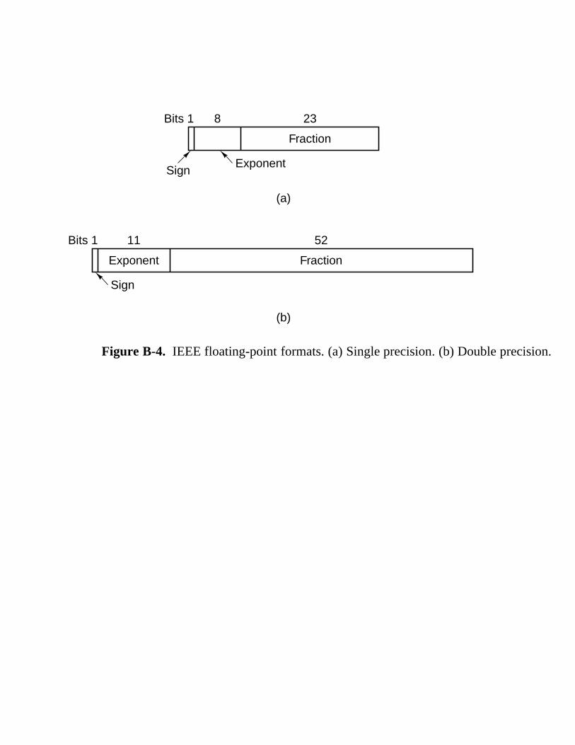
Bits 1
Bits 1
Sign
Sign
8 23
Fraction
Fraction
Exponent
(a)
(b)
11 52
Exponent
Figure B-4. IEEE floating-point formats. (a) Single precision. (b) Double precision.

22222222222222222222222222222222222222222222222222222222222222222222222Item Single precision Double precision22222222222222222222222222222222222222222222222222222222222222222222222
Bits in sign 1 122222222222222222222222222222222222222222222222222222222222222222222222Bits in exponent 8 1122222222222222222222222222222222222222222222222222222222222222222222222Bits in fraction 23 5222222222222222222222222222222222222222222222222222222222222222222222222Bits, total 32 6422222222222222222222222222222222222222222222222222222222222222222222222Exponent system Excess 127 Excess 102322222222222222222222222222222222222222222222222222222222222222222222222Exponent range −126 to +127 −1022 to +102322222222222222222222222222222222222222222222222222222222222222222222222Smallest normalized number 2−126 2−102222222222222222222222222222222222222222222222222222222222222222222222222Largest normalized number approx. 2128 approx. 2102422222222222222222222222222222222222222222222222222222222222222222222222Decimal range approx. 10−38 to 1038 approx. 10−308 to 1030822222222222222222222222222222222222222222222222222222222222222222222222Smallest denormalized number approx. 10−45 approx. 10−324222222222222222222222222222222222222222222222222222222222222222222222221111111111111111111
1111111111111111111
1111111111111111111
1111111111111111111
Figure B-5. Characteristics of IEEE floating-point numbers.

Normalized
Denormalized
Zero
Sign bit
Infinity
Not a number
Any bit pattern
Any nonzero bit pattern
Any nonzero bit pattern
0
0
0
0 < Exp < Max
1 1 1…1 0
1 1 1…1
±
±
±
±
±
Figure B-6. IEEE numerical types.