Graduate Theses, Dissertations, and Problem Reports

2013

Structure Segmentation and Transfer Faults in the Marcellus Structure Segmentation and Transfer Faults in the Marcellus

Shale, Clearfield County, Pennsylvania: Implications for Gas Shale, Clearfield County, Pennsylvania: Implications for Gas

Recovery Efficiency and Risk Assessment Using 3D Seismic Recovery Efficiency and Risk Assessment Using 3D Seismic

Attribute Analysis Attribute Analysis

Emily D. Roberts West Virginia University

Follow this and additional works at: https://researchrepository.wvu.edu/etd

Recommended Citation Recommended Citation Roberts, Emily D., "Structure Segmentation and Transfer Faults in the Marcellus Shale, Clearfield County, Pennsylvania: Implications for Gas Recovery Efficiency and Risk Assessment Using 3D Seismic Attribute Analysis" (2013). Graduate Theses, Dissertations, and Problem Reports. 221. https://researchrepository.wvu.edu/etd/221

This Thesis is protected by copyright and/or related rights. It has been brought to you by the The Research Repository @ WVU with permission from the rights-holder(s). You are free to use this Thesis in any way that is permitted by the copyright and related rights legislation that applies to your use. For other uses you must obtain permission from the rights-holder(s) directly, unless additional rights are indicated by a Creative Commons license in the record and/ or on the work itself. This Thesis has been accepted for inclusion in WVU Graduate Theses, Dissertations, and Problem Reports collection by an authorized administrator of The Research Repository @ WVU. For more information, please contact researchrepository@mail.wvu.edu.

Structure Segmentation and Transfer Faults in the Marcellus Shale, Clearfield

County, Pennsylvania: Implications for Gas Recovery Efficiency and Risk

Assessment Using 3D Seismic Attribute Analysis

Emily D. Roberts

Thesis submitted to the Eberly College of Arts and Sciences

at West Virginia University

in partial fulfillment of the requirements for the degree of

Master of Science in Geology

Dengliang Gao, Ph.D., Chair

Timothy R. Carr, Ph.D. Thomas H. Wilson, Ph.D.

Peter Sullivan, M.S.

Department of Geology and Geography

Morgantown, West Virginia 2013

Keywords: Marcellus Shale, Appalachian Basin, Structural Discontinuity, Fractures,

Hydraulic Fracture Stimulation, 3D Seismic Attributes

Copyright 2013 Emily D. Roberts

ABSTRACT

Structure Segmentation and Transfer Faults in the Marcellus Shale, Clearfield

County, Pennsylvania: Implications for Gas Recovery Efficiency and Risk Assessment

Using 3D Seismic Attribute Analysis

Emily D. Roberts

The Marcellus Shale has become an important unconventional gas reservoir in the oil

and gas industry. Fractures within this organic-rich black shale serve as an important

component of porosity and permeability useful in enhancing production. Horizontal

drilling is the primary approach for extracting hydrocarbons in the Marcellus Shale.

Typically, wells are drilled perpendicular to natural fractures in an attempt to intersect

fractures for effective hydraulic stimulation. If the fractures are contained within the shale,

then hydraulic fracturing can enhance permeability by further breaking the already

weakened rock. However, natural fractures can affect hydraulic stimulations by absorbing

and/or redirecting the energy away from the wellbore, causing a decreased efficiency in

gas recovery, as has been the case for the Clearfield County, Pennsylvania study area.

Estimating appropriate distances away from faults and fractures, which may limit

hydrocarbon recovery, is essential to reducing the risk of injection fluid migration along

these faults. In an attempt to mitigate the negative influences of natural fractures on

hydrocarbon extraction within the Marcellus Shale, fractures were analyzed through the

aid of both traditional and advanced seismic attributes including variance, curvature, ant

tracking, and waveform model regression. Through the integration of well log

interpretations and seismic data, a detailed assessment of structural discontinuities that

may decrease the recovery efficiency of hydrocarbons was conducted. High-quality 3D

seismic data in Central Pennsylvania show regional folds and thrusts above the major

detachment interval of the Salina Salt. In addition to the regional detachment folds and

thrusts, cross-regional, northwest-trending lineaments were mapped. These lineaments

may pose a threat to hydrocarbon productivity and recovery efficiency due to faults and

fractures acting as paths of least resistance for induced hydraulic stimulation fluids. These

lineaments may represent major transfer faults that serve as pathways for hydraulic fluid

migration. Detection and evaluation of fracture orientation and intensity and emphasis on

the relationship between fracture intensity and production potential is of high interest in

the study area as it entails significant time and cost implications for both conventional and

unconventional hydrocarbon exploration and production.

iii

ACKNOWLEDGEMENTS

I would like to thank my thesis committee members Dengliang Gao, Tim Carr, Tom

Wilson, and Pete Sullivan for their guidance and encouragement throughout my research

efforts. Thank you to Dr. Wilson for seeing the potential in me and accepting me into graduate

school at WVU and to Dr. Carr for suggesting I work with this dataset. Finally, thank you Dr.

Gao for becoming my advisor and professional mentor and for the overwhelming support of my

project and ideas over the years.

Thank you to Energy Corporation of America for funding this project and allowing

me to work with their seismic data volume and well logs, specifically Pete Sullivan and

Chad Cunningham for their advice and technical assistance with the dataset. Finally, I want

to thank the National Energy Technology Laboratory for additional funding (to Dengliang

Gao), under the contract: RES1000023/TRN217U, and activity ID: 4000.2.651.072.001.

iv

TABLE OF CONTENTS ABSTRACT .................................................................................................................................................................................. ii

ACKNOWLEDGEMENTS ....................................................................................................................................................... iii

TABLE OF CONTENTS ........................................................................................................................................................... iv

LIST OF FIGURES .................................................................................................................................................................... vi

1. INTRODUCTION .................................................................................................................................................................. 2

1.1 Fractures and Hydrocarbon Recovery Implications ...................................................................... 2

1.2 Objectives and Approach .................................................................................................................. 2

2. FRACTURES AND MECHANISMS OF FRACTURE DEVELOPMENT ................................................................. 4

2.1 Introduction ....................................................................................................................................... 4

2.2 Fracture Types ................................................................................................................................... 5

2.2.1 Joints ............................................................................................................................................ 5

2.2.2 Faults ........................................................................................................................................... 6

2.2.3 Fracture Swarms ........................................................................................................................ 7

2.3 Mechanism of Fracture Development ............................................................................................. 8

2.4 Fault Damage/Deformation Zones .................................................................................................. 8

2.5 Regional and Local Stresses ............................................................................................................. 9

3. SEISMIC ATTRIBUTES ................................................................................................................................................... 10

3.1 Introduction ..................................................................................................................................... 10

3.2 Attributes Defined ........................................................................................................................... 10

3.2.1 Curvature .................................................................................................................................. 11

3.2.2 Variance .................................................................................................................................... 12

3.2.3 Ant Tracking from Variance .................................................................................................... 12

3.2.4 Waveform Model Regression .................................................................................................. 14

4. GEOLOGIC SETTING ........................................................................................................................................................ 15

4.1 Introduction ..................................................................................................................................... 15

4.2 Tectonic History .............................................................................................................................. 16

4.3 Stratigraphy ..................................................................................................................................... 20

4.4 Structure .......................................................................................................................................... 22

5. PREVIOUS WORK .............................................................................................................................................................. 29

v

6. DATA AND METHODOLOGY ......................................................................................................................................... 31

6.1 Well Log Analysis ............................................................................................................................ 31

6.2 Seismic Attribute Analysis .............................................................................................................. 33

6.3 Seismic Well Tie .............................................................................................................................. 34

7. RESULTS ............................................................................................................................................................................... 36

7.1 Geologic Structure and Stratigraphy Interpretations .................................................................. 36

7.2 Structural Attribute Analysis.......................................................................................................... 47

7.3 Correlation of Seismic Data with FMI Log Data ............................................................................ 77

7.4 Correlation of Seismic Data with Surface Fracture Orientations and Breakout Data ................ 81

8. CONCLUSIONS .................................................................................................................................................................... 83

9. REFERENCES ...................................................................................................................................................................... 88

vi

LIST OF FIGURES

Figure 1: Paleogeography in the Middle Devonian (385Ma). Approximate location of study area ............................................................................................................................................................................. 4

Figure 2: Block diagram sketches showing the different types of faults ......................................... 7

Figure 3: 2D representation of curvature attribute .............................................................................. 12

Figure 4: The tectonic evolution of the Appalachian basin ............................................................... 19

Figure 5: Stratigraphic column showing the Middle Devonian interval ....................................... 21

Figure 6: Paleo-depostional environments in the Middle Devonian ............................................. 21

Figure 7: Structural contours on top of Onondaga Limestone ......................................................... 25

Figure 8: Thickness map of Marcellus Shale ........................................................................................... 25

Figure 9: Generalized stratigraphic cross-section across western Pennsylvania and eastern Ohio ......................................................................................................................................................................... 26

Figure 10: Major lineaments as observed from gravity anomalies throughout Pennsylvania ................................................................................................................................................................................... 26

Figure 11: Regional and local structure maps showing previously mapped lineaments from gravity anomaly and surface data................................................................................................................ 27

Figure 12: Strike-slip, transverse faulting in Clearfield County, Pennsylvania ......................... 28

Figure 13: Gamma ray logs from study area used for stratigraphic correlation ....................... 32

Figure 14: Well with sonic log used to make synthetic seismogram ............................................. 34

Figure 15: Synthetic seismogram from well ............................................................................................ 35

Figure 16: Example of well log and seismic data after time depth conversion from synthetic seismogram .......................................................................................................................................................... 35

Figure 17: Inline 48 showing structure and stratigraphy throughout study area. .................. 38

Figure 18: Structure time map of Onondaga Limestone surface with wells (TWT). ............... 38

Figure 19: Structure time map of Tully Limestone (TWT). ............................................................... 39

Figure 20: Structure time map of Marcellus Shale (TWT). ................................................................ 40

vii

Figure 21: Structure time map of Oriskany Sandstone (TWT). ....................................................... 41

Figure 22: Structure time map on Salina Salt (TWT). .......................................................................... 42

Figure 23: Tully Limestone isochron thickness map (TWT). ............................................................ 43

Figure 24: Marcellus Shale isochron thickness map (TWT). ............................................................. 44

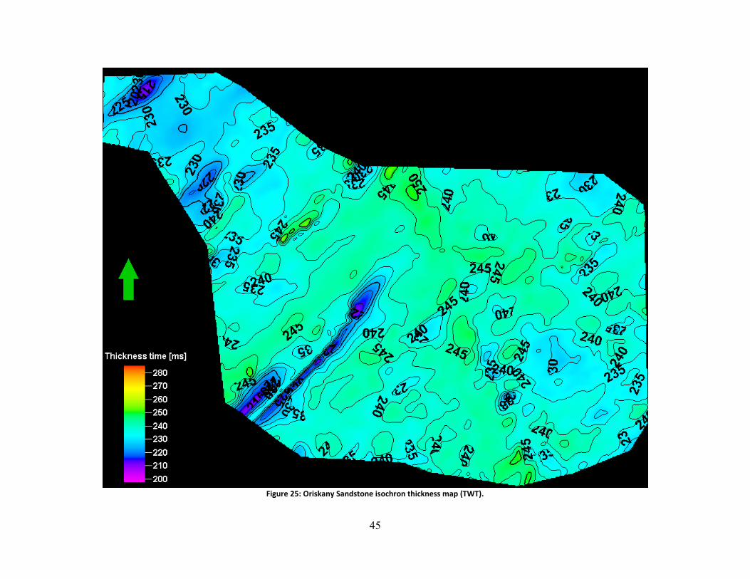
Figure 25: Oriskany Sandstone isochron thickness map (TWT). .................................................... 45

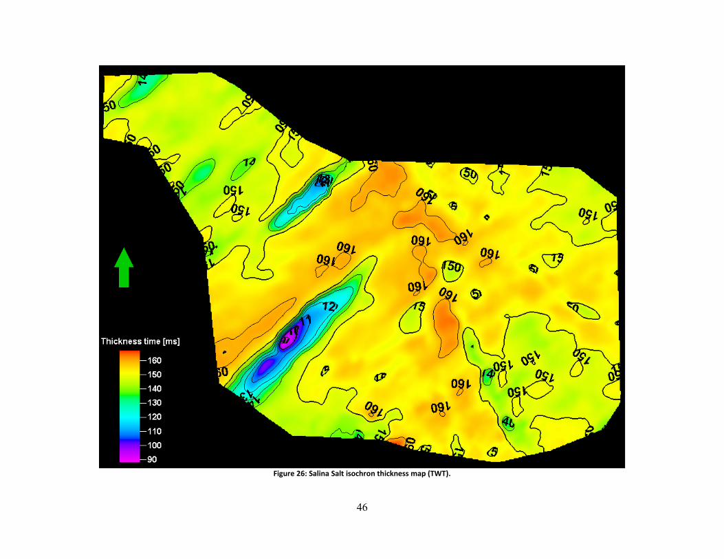
Figure 26: Salina Salt isochron thickness map (TWT). ....................................................................... 46

Figure 27: WMR attribute with uninterpreted inline A1 .................................................................... 53

Figure 28: WMR attribute with interpreted inline A1 ......................................................................... 54

Figure 29: WMR attribute with uninterpreted inline A2 and A3 .................................................... 55

Figure 30: WMR attribute with interpreted inline A2 and A3.......................................................... 56

Figure 31: WMR attribute with uninterpreted inline B1 and B2 .................................................... 57

Figure 32: WMR attribute with interpreted inline B1 and B2 .......................................................... 58

Figure 33: Curvature attribute for time slice (~975ms) of the Tully Limestone ...................... 59

Figure 34: Curvature attribute for time slice (~1058ms) of the Marcellus Shale .................... 60

Figure 35: Curvature attribute for time slice (~1080ms) near the Oriskany Sandstone ...... 61

Figure 36: Curvature attribute for time slice (~1150ms) above the Salina Salt ....................... 62

Figure 37: Most extreme curvature attribute for time slice (~975ms) of the Tully Limestone ................................................................................................................................................................................... 63

Figure 38: Most extreme curvature attribute for time slice (~1058ms) of the Marcellus Shale ........................................................................................................................................................................ 64

Figure 39: Most extreme curvature attribute for time slice (~1080ms) near the Oriskany Sandstone .............................................................................................................................................................. 65

Figure 40: Most extreme curvature attribute for time slice (~1150ms) above the Salina Salt ................................................................................................................................................................................... 66

Figure 41: Variance attribute for time slice (~974ms) of the Tully Limestone ........................ 67

Figure 42: Variance attribute for time slice (~1058ms) near the Marcellus Shale ................ 68

Figure 43: Variance attribute for time slice (~1080ms) near the Oriskany Sandstone ......... 69

viii

Figure 44: Variance attribute for time slice (~1150ms) above the Salina Salt ......................... 70

Figure 45: Ant tracking attribute for time slice (~975ms) of the Tully Limestone. ................ 71

Figure 46: Ant tracking attribute for time slice (~1058ms) of the Marcellus Shale ............... 72

Figure 47: Ant tracking attribute for time slice (~1080ms) near the Oriskany Sandstone . 73

Figure 48: Ant tracking attribute for time slice (~1150ms) above the Salina Salt .................. 74

Figure 49: Original seismic amplitude data for time slice (~1080ms) near the Oriskany Sandstone with ant tracking from variance overlain ........................................................................... 75

Figure 50: Variance attribute data for time slice (~1080ms) near the Oriskany Sandstone with ant tracking from variance overlain ................................................................................................. 76

Figure 51: Formation Microimager log from a well outside of the 3D seismic dataset ......... 78

Figure 52: Fracture descriptions interpreted from the FMI log ...................................................... 79

Figure 53: FMI log data .................................................................................................................................... 79

Figure 54: Automatic fault extraction within the Middle Devonian interval.............................. 80

Figure 55: Automatic fault extraction data .............................................................................................. 80

Figure 56: Map of present day stresses in relation to location of study area ............................. 82

2

1. INTRODUCTION

1.1 Fractures and Hydrocarbon Recovery Implications

Present technological advances in geophysics, particularly in the field of seismic

imaging, has allowed geoscientists to identify both major and minor scale structures that

are buried deep beneath the surface and lack surface expression. However, the benefits of

seismic imaging go far beyond creating a visual image of the subsurface. Technological

advances, an improved understanding of seismic wave propagation, and enhanced

attribute analysis has led to increasingly more reliable and geologically significant

interpretations of seismic scale and sub-seismic scale features such as fracture swarms or

fracture sweet spots. (Hart, Pearson, and Rawling, 2002)

Current economic demands for clean energy alternatives, along with increasing

advancements in drilling technologies, have made the Marcellus Shale a leader in natural

gas plays. Several fracture sets are consistent throughout the Marcellus Shale and serve as

an important component for enhancing production (Engelder, Lash, and Uzcategui, 2009).

However, connecting faults and fractures have the potential to hinder gas recovery in the

study area if hydraulic injection fluids are directed away from the target formation and

wellbore.

1.2 Objectives and Approach

The purpose of this study is to determine if both major and minor structures, such

as faults and fractures, fracture swarms or networks, can be located within the Marcellus

Shale through the use of complex seismic attribute analysis. An emphasis on the

relationship between fractures and faults, particularly strike-slip faults with deep

3

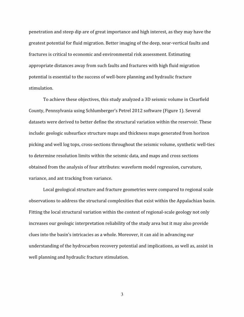
penetration and steep dip are of great importance and high interest, as they may have the

greatest potential for fluid migration. Better imaging of the deep, near-vertical faults and

fractures is critical to economic and environmental risk assessment. Estimating

appropriate distances away from such faults and fractures with high fluid migration

potential is essential to the success of well-bore planning and hydraulic fracture

stimulation.

To achieve these objectives, this study analyzed a 3D seismic volume in Clearfield

County, Pennsylvania using Schlumberger’s Petrel 2012 software (Figure 1). Several

datasets were derived to better define the structural variation within the reservoir. These

include: geologic subsurface structure maps and thickness maps generated from horizon

picking and well log tops, cross-sections throughout the seismic volume, synthetic well-ties

to determine resolution limits within the seismic data, and maps and cross sections

obtained from the analysis of four attributes: waveform model regression, curvature,

variance, and ant tracking from variance.

Local geological structure and fracture geometries were compared to regional scale

observations to address the structural complexities that exist within the Appalachian basin.

Fitting the local structural variation within the context of regional-scale geology not only

increases our geologic interpretation reliability of the study area but it may also provide

clues into the basin’s intricacies as a whole. Moreover, it can aid in advancing our

understanding of the hydrocarbon recovery potential and implications, as well as, assist in

well planning and hydraulic fracture stimulation.

4

Figure 1: Paleogeography in the Middle Devonian (385Ma). Approximate location of study area

indicated by yellow box. (Modified from Blakey, 2008)

2. FRACTURES AND MECHANISMS OF FRACTURE DEVELOPMENT

2.1 Introduction

To establish a framework for understanding the fracture systems within the

Appalachian basin and the Marcellus Shale, it is necessary to define fractures and discuss

their mechanisms for development. In geology, the term fracture is generally used to refer

to two main groups of structural features: joints and faults (Van der Pluijm and Marshak,

2004). Typically, joints and faults form in sets or groups, referred to as fracture swarms or

fracture networks. These fracture swarms are important to hydrocarbon recovery because

they can provide conduits for subsurface fluid migration or, if cemented or mineralized, can

compartmentalize reservoirs by forming impenetrable barriers to fluid flow (Hsieh et al.,

5

1993). The primary focus of this study is on the identification of such fracture swarms or

fracture networks through seismic attribute analysis to aid in the enhancement of

hydrocarbon recovery efficiency.

2.2 Fracture Types

2.2.1 Joints

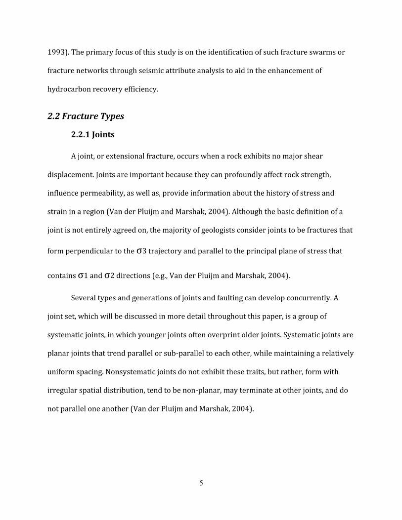
A joint, or extensional fracture, occurs when a rock exhibits no major shear

displacement. Joints are important because they can profoundly affect rock strength,

influence permeability, as well as, provide information about the history of stress and

strain in a region (Van der Pluijm and Marshak, 2004). Although the basic definition of a

joint is not entirely agreed on, the majority of geologists consider joints to be fractures that

form perpendicular to the σ3 trajectory and parallel to the principal plane of stress that

contains σ1 and σ2 directions (e.g., Van der Pluijm and Marshak, 2004).

Several types and generations of joints and faulting can develop concurrently. A

joint set, which will be discussed in more detail throughout this paper, is a group of

systematic joints, in which younger joints often overprint older joints. Systematic joints are

planar joints that trend parallel or sub-parallel to each other, while maintaining a relatively

uniform spacing. Nonsystematic joints do not exhibit these traits, but rather, form with

irregular spatial distribution, tend to be non-planar, may terminate at other joints, and do

not parallel one another (Van der Pluijm and Marshak, 2004).

6

2.2.2 Faults

Faults are fractures along which shear displacement has occurred. Faults may be

associated with either extensional or contractional strain and include dip slip faulting, such

as normal faulting, reverse faulting or thrust faulting (a low angle reverse fault), and strike-

slip faulting (Figure 2). The shear sense of faulting is described on a dip-slip fault with

reference to a horizontal line on the fault by describing the movement as either hanging-

wall up (reverse or thrust faulting) or hanging-wall down (normal faulting) with respect to

the footwall. When the shear sense is parallel to the fault strike and the line representing

slip direction has a rake (pitch) in the fault plane of less than 10 degrees, we consider this

to be a strike-slip fault. Strike-slip faults tend to be steeply dipping to vertical (Van der

Pluijm and Marshak, 2004).

Anderson (1951) defines normal faults as fractures associated with extension and a

vertical σ1 orientation and reverse faults as fractures associated with compression and a

horizontal σ1 orientation. He characterizes strike-slip faults as fractures associated with

lateral displacement or block rotation with σ1 and σ3 being horizontal. Oblique slip

faulting occurs when both dip-slip and strike-slip displacement is a result of inclined stress

axes or the inhomogeneity of strength or elastic properties (Bott, 1959).

7

Figure 2: Block diagram sketches showing the different types of faults. (From Van der Pluijm and Marshak, 2004)

2.2.3 Fracture Swarms

Olsen (2004) describes fracture swarms as groups of tightly-spaced fractures that

are considered the exception to the widely accepted rule that fracture spacing in

sedimentary rocks is proportional to the mechanical layer thickness. Such fracture swarms

occur in areas experiencing regional tectonic stresses. Fracture swarms are also thought to

occur in local stress field interactions which may cause propagating fractures to

communicate (Olsen, 2004).

Cooke and Underwood (2000) suggest that rather than mechanical drivers alone,

stress fields associated around a propagating fracture tip represent the point of maximum

tension and are more likely to influence the direction of the fractures’ continuing

propagation. As a result, the fracture tip will likely be attracted toward another fracture

since this will be a zone of preexisting weakness, than to continue to propagate through an

unfractured zone. Fracture swarms may significantly enhance hydrocarbon recovery in the

8

Marcellus Shale, since it has been suggested that fractures can increase permeability when

hydraulically stimulated.

2.3 Mechanism of Fracture Development

Faults and joints represent the response of rock to the effects of stress and strain

being applied to the rock. In the event that the elastic strain on a surface or plane reaches

or exceeds the critical value, the rock will fail and a fracture will form (Van der Pluijm and

Marshak, 2004). Several parameters will influence whether a fault or joint will develop.

Such parameters include the orientation of the principal stress axes (σ1, σ2 andσ3),

surface planarity of the fracture, rock brittleness, and the magnitude of shear strains being

accommodated by the surface undergoing stress (Van der Pluijm and Marshak, 2004).

Faulting only occurs when the differential stress is not equal to zero (σ1=σ2=σ3). A

relationship between fault orientations and the trajectories of principal stresses during a

tectonic event can be made because the shear-stress magnitude on a plane will change as a

function of the plane’s orientation with respect to principal stresses (Van der Pluijm and

Marshak, 2004). This relationship is important for understanding paleo-stresses and their

influence on fault trends, which will be discussed in chapter 7.

2.4 Fault Damage/Deformation Zones

To better define the types of structures observed in this study and the vocabulary

that will be used to describe them, it is important to distinguish between faults and fault

damage zones. For the purpose of this study, fault damage zones are considered to be zones

of deformation around major faults, in which greater fracture density occurs relative to the

9

area surrounding it. Chapter 7 will provide examples of potential damage/deformation

zones in our study area.

Shipton and Cowie (2003) consider fault damage zones to contain “subsidiary

structures” that occur for a number of reasons, including bedding flexure, repeated fault

slip, and enhanced stress and strain from zones of adjacent faults and fault connectivity.

The systematic geometries of damage zones may aid in the prediction of sub-seismic fault

distribution, as well as, fluid migration pathways. Thus, it is imperative that fault damage

zones can play a huge role in interpreting the geology and structural complexity of the

Clearfield, Pennsylvania study area (Figure 1) and the potential influence of fault damage

zones.

2.5 Regional and Local Stresses

One of the primary objectives for this work included a qualitative comparison

between regional stresses and their influence on the local stresses and the role they have

on the formation of geologic structures observed within our study area. Stearns and

Friedman (1972) related the regional structural style of joints and faults to inferred local

stress regimes expected during faulting and folding. However, it is inevitable that

comparisons between local and regional stresses will not always prove to be consistent,

but rather, may vary significantly depending on the structural regime and variation of local

stress throughout the basin (i.e. location), among other factors. Still, it is noteworthy to

take into account these comparisons, as they only lend further insight into the factors

influencing the local geology of the dataset.

10

3. SEISMIC ATTRIBUTES

3.1 Introduction

Seismic attributes contain fundamental pieces of information within a recorded

seismic trace that can be used to enhance subsurface visualization and interpretation

(Chopra and Marfurt, 2007). Seismic attributes serve as a useful tool for petroleum

industry exploration and field development. Attributes analysis includes the assessment of

structures such as faults and folds (traps), stratigraphy, including lateral variation in

lithology and thickness, and reservoir properties, such as porosity and permeability and

hydrocarbon indicators.

In order to perform a 3D seismic attribute analysis, attributes most readily

prevalent to structural analysis were used. Since the main objective of this study centered

on assessing fracture locations, orientations, intensities, and connectivity of fracture

networks, waveform model regression (WMR), curvature, variance, and ant tracking

structural attributes were used. This allowed for a more reliable interpretation of the

subsurface, including fault and fracture network delineation, to address issues of fluid

migration potential and hydrocarbon recovery efficiency.

3.2 Attributes Defined

A seismic attribute is a quantitative measure of a seismic data property or

properties that can be measured along a single seismic trace or multiple traces at one

instant in time (time slice) or summed over a time interval (interpreted horizon/surface,

cross-section) (Schlumberger, 2013). Attributes can be divided into several categories,

11

including pre-stack or post-stack attributes, instantaneous attributes, wavelet attributes,

physical attributes, geometrical attributes, reflective attributes and transmissive attributes

(Brown, 2004, 2001, 1996; Taner, 2001).

Attributes applied to the 3D seismic survey in this study include curvature, variance

and waveform model regression. Ant tracking, Schlumberger’s automated discontinuity

attribute, was applied to trace faults and fractures from the variance attribute. All of the

aforementioned attributes are considered geometrical (or structural) attributes, and will

be detailed in the following sections.

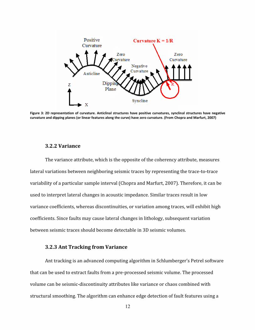
3.2.1 Curvature

The curvature attribute is a measure of the reflector geometry of a given seismic

trace and is defined in two dimensions as the radius of a circle tangent to a curve,

independent of bulk rotations and translations of the reflector (Chopra and Marfurt, 2007).

Thus, positive and negative curvature values are inferred to be anticlines and synclines,

respectively. Zero curvature values represent areas along the curve associated with

straight lines (Figure 3).

Curvature has been found to serve as a useful attribute for delineating faults,

fracture swarms, and folds. Chopra and Marfurt (2007) suggest that curvature maps

accurately depict the present-day subsurface structure, particularly faults and zones of

flexure (i.e. fracture swarms). Most positive and most negative values are thought to be the

most unambiguous of the curvature measurements in highlighting faults and folds.

12

Figure 3: 2D representation of curvature. Anticlinal structures have positive curvatures, synclinal structures have negative curvature and dipping planes (or linear features along the curve) have zero curvature. (From Chopra and Marfurt, 2007)

3.2.2 Variance

The variance attribute, which is the opposite of the coherency attribute, measures

lateral variations between neighboring seismic traces by representing the trace-to-trace

variability of a particular sample interval (Chopra and Marfurt, 2007). Therefore, it can be

used to interpret lateral changes in acoustic impedance. Similar traces result in low

variance coefficients, whereas discontinuities, or variation among traces, will exhibit high

coefficients. Since faults may cause lateral changes in lithology, subsequent variation

between seismic traces should become detectable in 3D seismic volumes.

3.2.3 Ant Tracking from Variance

Ant tracking is an advanced computing algorithm in Schlumberger’s Petrel software

that can be used to extract faults from a pre-processed seismic volume. The processed

volume can be seismic-discontinuity attributes like variance or chaos combined with

structural smoothing. The algorithm can enhance edge detection of fault features using a

13

discriminative and iterative process that replicates natural ant behaviors (Chopra and

Marfurt, 2007).

The ant tracking workflow consists of a number of independent steps. First, a pre-

conditioned (structurally smoothed) seismic volume with an edge detection algorithm

applied (e.g. variance) needs to be generated. Structural smoothing will help to reduce the

noise in the seismic data while the algorithm will enhance the spatial discontinuities. Then,

the ant tracking attribute can be applied to the variance seismic volume and faults can be

extracted. Faults must then be validated and edited for erroneous faults, which may have

been an artifact from noise or correlate with reflection events, rather than faults. Also,

horizontal features associated with stratigraphy can be filtered out to further increase

accuracy for modeling fault interpretations.

There are several benefits to using the ant tracking attribute. Ant tracking can

increase structural accuracy and detail providing unbiased, repeatable mapping of

discontinuities. Furthermore, the algorithm can produce highly detailed fault

interpretations, which must be quality controlled, but allow for the interpreter to efficiently

enhance the detail of the fault interpretation. Ant tracking is also useful for checking the

accuracy with which faults have been interpreted, thus enhancing the interpreter’s

confidence. For this reason, interpreted fault surfaces may be compared to fault surfaces

that had been tracked by the automated process as a form of secondary calibration (Chopra

and Marfurt, 2007).

14

3.2.4 Waveform Model Regression

A new and advanced attribute called a constant-phase waveform model regression

WMR) was applied to the 3D seismic volume to better highlight structural features within

the dataset. The WMR algorithm applies a linear least-squares regression to adjust

similarity between a wavelet model and seismic data (Gao, 2013, 2012a, 2004, 2002;

Donahoe and Gao, 2012; Donahoe, 2011). The WMR attribute is evaluated at each sample

located along each wiggle trace and converts the regular wiggle trace into a structurally-

enhanced attribute. The waveform frequency is then increased through waveform to

constant phase correlation and by calculating the absolute correlation coefficient (Gao,

2013, 2012a, 2004, 2002; Donahoe and Gao, 2012; Donahoe, 2011). The signal to noise

ratio is then enhanced by the linear least-squares regression, in turn, allowing for

improved visualization and mapping of structural features such as faults and folds.

The WMR attribute can be used to characterize structures, facies and reservoir

properties from seismic data that might not be easily recognizable from regular seismic

amplitude data alone (Gao, 2013, 2012a, 2004, 2002; Donahoe and Gao, 2012; Donahoe,

2011). In this study, the constant-phase WMR attribute was applied to the seismic data to

better visualize and interpret structures in both map view and cross-sectional view.

Structural analysis, including fault locations, extent, and connectivity is more robust by

using this advanced, seismic waveform-based attribute. A more detailed and accurate

interpretation was possible through the use of the WMR attribute in this 3D survey.

15

4. GEOLOGIC SETTING

4.1 Introduction

Most structures throughout Pennsylvania can be genetically related to four main

tectonic orogenic episodes in the Appalachian foreland basin. These four events include the

Grenville, Taconic, Acadian, and Allegheny orogenies, which initiated during the Ordovician

and extended throughout the Pennsylvanian, dominantly controlling the derivation of the

central Appalachian basin. Prior to the foreland basin orogenesis, extension in

Precambrian-Cambrian brought about a major rift system, known as the Rome trough that

extends throughout the area of interest (Kulander and Ryder, 2005; Edmonds, 2004;

Hibbard, 2004; Gao, Shumaker, and Wilson, 2000; Wilson, 2000; Gao and Shumaker, 1996;

Shumaker and Wilson, 1996; Kulander and Dean, 1986, 1980).

The overprinting of these events has complicated the structural style and history of

the basin. Both the Cambrian basement-involved rift structure and the post Silurian (post-

salt) detachment structures are complicated by regional and cross-regional lineaments.

The regional lineaments are trending to the northeast, whereas the cross-regional

lineaments trend in variable directions (Gao et al., 2000; Gao and Shumaker, 1996). Some

cross-regional lineaments are reported to be orthogonal to the strike of the regional

structures called cross-strike discontinuities (Shultz, 1999; Wheeler, 1980; Wilson, 1980).

Some are oblique to the regional trend such as the 38th parallel, the Burning-Mann, and the

40th parallel lineaments (Gao et al., 2000). These cross-regional lineaments, oblique or

orthogonal, basement-involved or detached, make the Rome trough and the foreland basin

structures variable along the regional trend (Gao et al., 2000; Gao and Shumaker, 1996).

16

Such along-axis variation and segmentation have important implications for tectonics,

sedimentation, and hydrocarbon accumulation in the foreland basin (Gao et al., 2000). In

unconventional shale-gas exploration, an understanding of the polyhistory of the basin, as

well as structure and stratigraphy associated with it, is necessary for evaluating potential

for fracture development and reactivation and movement along pre-existing faults and

zones of weakness. Thus, detecting regional and cross-regional faults and fractures and

unraveling their polyhistory is fundamental to the success for both conventional and

unconventional energy exploration and production.

4.2 Tectonic History

The Grenville Orogeny occurred during the late Precambrian and is expressed by

complex deformation, including primary flow foliation, gneissic structures, and recumbent

isoclinal folds (Shultz, 1999) (Figure 4). Few large-scale structures have been observed or

documented from this orogeny. However, low angle faulting in basement rock has been

observed from seismic data in the Appalachian Plateau region (Shultz, 1999). These

features may contribute minimally to structural deformation in overlying strata throughout

the region.

The Appalachian cycle of deformation and sedimentation largely began in the late

Precambrian (about 750 Ma) era when rifting associated with extension created the

Iapetus Ocean and the Rome trough. Rifting that occurred throughout the Early-Middle

Cambrian brought about a series of grabens that extend throughout western Pennsylvania

(Figure 4) (Kulander and Ryder, 2005; Edmonds, 2004; Hibbard, 2004; Gao et al., 2000;

Wilson, 2000; Gao and Shumaker, 1996; Shumaker and Wilson, 1996; Kulander and Dean,

17

1986, 1980). Several lineaments, particularly step down normal faulting to the east, are

associated with these rifting events and have been observed in Precambrian basement rock

from seismic data (Hibbard, 2004).

Following these rifting events, a brief period of thermal subsidence and passive

margin tectonics persisted (Shultz, 1999) up until the Late Ordovician when the Taconic

Orogeny initiated (Figure 4). This orogeny marked the beginning of the structural

deformation seen within the Appalachian basin today. The Taconic orogeny resulted from

the collision of continental arcs with the eastern margin of Laurentia, causing plate

subduction. This orogeny created several pronounced structures throughout the basin,

including overlapping recumbent folds in southeast Pennsylvania and southeast-dipping

monoclinal flexures in western Pennsylvania (Shultz, 1999).

Effects of the Taconic Orogeny continued into the Early Silurian, when subduction

halted and the erosion of the newly-formed orogenic belt (Taconic mountains from

recycled Iapetus Terrane) began (Figure 4). As the Taconic mountains eroded throughout

the Late Silurian, the sea transgressed eastward, allowing for clastic and carbonate

deposition. Marine shelf environments and tectonically inactive conditions persisted into

the Early Devonian, depositing shale, carbonate, and evaporite (Shultz, 1999).

From the Devonian to Early Mississippian, the Acadian Orogeny governed the

evolution of the central Appalachian basin (Shultz, 1999) (Figure 4). A second influx of

detrital sediment was introduced into the basin from orogenic highlands created by the

Acadian Orogeny, which allowed for Middle Devonian rock units, including the Onondaga

Limestone and Hamilton Group (includes Marcellus Shale), to accumulate in basinal marine

environments (Shultz, 1999).

18

The Late Devonian Acadian Orogeny produced only minor structures in the

Pennsylvania, such as upfaulted blocks of the Precambrian basement complex and fracture

cleavage in some rock units. However, small anticlinal structures resulted from the

extension in the Appalachian Plateau that mobilized rock salt of the Silurian Salina Group

along Taconic monoclines. These structures are similar to those observed within this study.

The Appalachian cycle of deformation and sedimentation climaxed during the

Permian with the Allegheny Orogeny. This orogeny began in late Mississippian and

extended throughout the Early Permian. Complex deformation resulted from the collision

of Gondwana and the Peri-Gondwana continents, ultimately leading to the assembly of the

supercontinent Pangea (Shultz, 1999) (Figure 4).

Of particular significance is the non-emergent decollement in the Upper Cambrian

section that allowed tectonic transport of all the rock units in the southeast part of the

basin to the northwest (Shultz, 1999), thus contributing to crustal shortening throughout

the basin. The great curving arc of major anticlines observed throughout Pennsylvania

formed as a result of the Allegheny Orogeny. The Allegheny Front marks the location

where the decollement climbed stratigraphically into the Silurian Salina Group. Rootless

duplex structures formed as anticlinoriums developed along high-angle splay faults and

Taconic nappes advanced along bounding thrust faults (Shultz, 1999).

The Taconic Orogeny is well preserved in the northern part of the basin but strongly

overprinted in the south by the Allegheny Orogeny. Hibbard (2004) suggests that accretion

in the northern Appalachians during the Middle and Late Paleozoic involved a strike-slip

component and areas of intense Silurian and Acadian deformation may be the result of

localized collisions where strike-slip motion was impeded by promontories. Hibbard’s

19

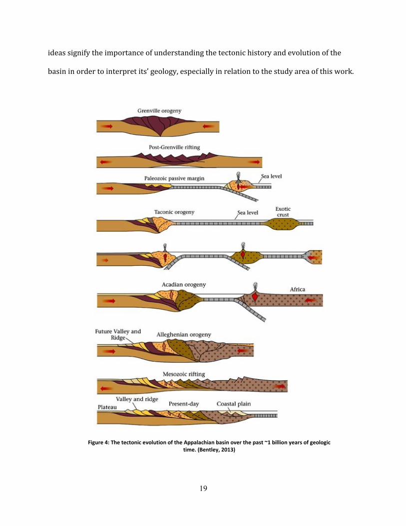
ideas signify the importance of understanding the tectonic history and evolution of the

basin in order to interpret its’ geology, especially in relation to the study area of this work.

Figure 4: The tectonic evolution of the Appalachian basin over the past ~1 billion years of geologic time. (Bentley, 2013)

20

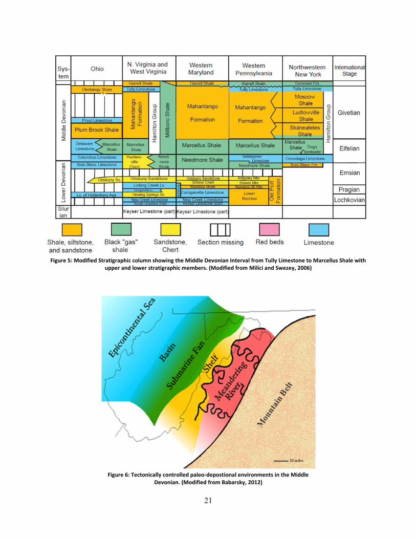
4.3 Stratigraphy

The Marcellus Shale is an organic-rich black shale that lies beneath the Mahantango

Formation. Together, these two formations make up what is referred to as the Hamilton

Group (Figure 5). The Hamilton Group is made up of shallow-marine deposits that include

intertonguing limestone, sandstones, coal, and shale (Zagorski, Bowman, Emery, and

Wrightstone, 2011). Above the Hamilton Group is the Tully Limestone and below, rests the

Onondaga Limestone and Oriskany Sandstone, respectively.

These sequences have been complicated by the nature of their deposition during

advances and retreats of a shallow epicontinental seaway (Figure 6). These transgressive-

regressive cycles may attribute to build-up and pinch-out sequences commonly observed

throughout the basin’s stratigraphy (Lash and Engelder, 2011). Boyce (2010) suggests

variations within sequences are a combination of short transgressive-regressive cycles that

were complicated by local structural highs and lows during time of deposition.

21

Figure 5: Modified Stratigraphic column showing the Middle Devonian Interval from Tully Limestone to Marcellus Shale with

upper and lower stratigraphic members. (Modified from Milici and Swezey, 2006)

Figure 6: Tectonically controlled paleo-depostional environments in the Middle

Devonian. (Modified from Babarsky, 2012)

22

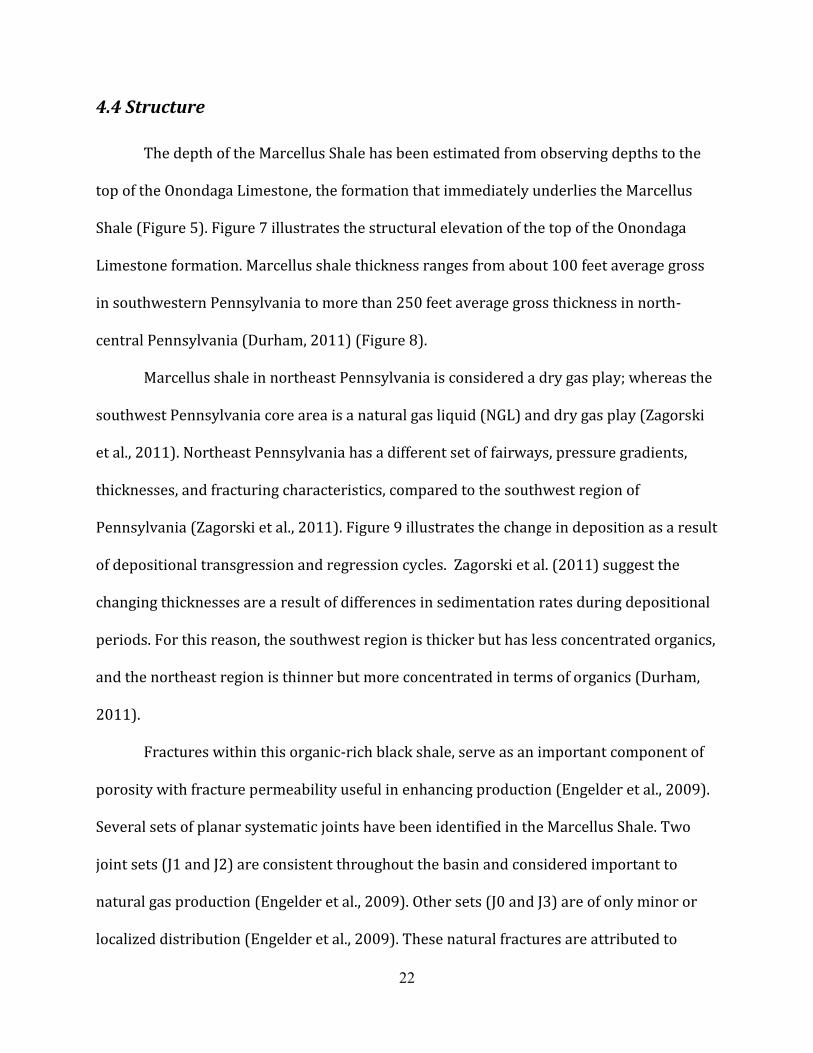
4.4 Structure

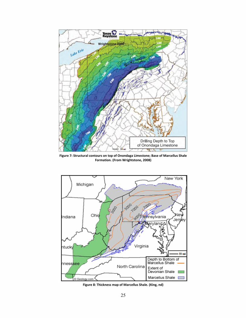
The depth of the Marcellus Shale has been estimated from observing depths to the

top of the Onondaga Limestone, the formation that immediately underlies the Marcellus

Shale (Figure 5). Figure 7 illustrates the structural elevation of the top of the Onondaga

Limestone formation. Marcellus shale thickness ranges from about 100 feet average gross

in southwestern Pennsylvania to more than 250 feet average gross thickness in north-

central Pennsylvania (Durham, 2011) (Figure 8).

Marcellus shale in northeast Pennsylvania is considered a dry gas play; whereas the

southwest Pennsylvania core area is a natural gas liquid (NGL) and dry gas play (Zagorski

et al., 2011). Northeast Pennsylvania has a different set of fairways, pressure gradients,

thicknesses, and fracturing characteristics, compared to the southwest region of

Pennsylvania (Zagorski et al., 2011). Figure 9 illustrates the change in deposition as a result

of depositional transgression and regression cycles. Zagorski et al. (2011) suggest the

changing thicknesses are a result of differences in sedimentation rates during depositional

periods. For this reason, the southwest region is thicker but has less concentrated organics,

and the northeast region is thinner but more concentrated in terms of organics (Durham,

2011).

Fractures within this organic-rich black shale, serve as an important component of

porosity with fracture permeability useful in enhancing production (Engelder et al., 2009).

Several sets of planar systematic joints have been identified in the Marcellus Shale. Two

joint sets (J1 and J2) are consistent throughout the basin and considered important to

natural gas production (Engelder et al., 2009). Other sets (J0 and J3) are of only minor or

localized distribution (Engelder et al., 2009). These natural fractures are attributed to

23

tectonic stresses, uplift and erosional forces, and mechanical compaction of the rocks, at

local and regional scales (Bruner and Smosna, 2011).

J1 joint set orientations have a characteristic ENE orientation with a consistent

strike between 60-75 degrees. This set is thought to be the primary joint set, having formed

prior to Allegheny folding. J1 joints are more closely spaced and cross-cut by the J2 joints.

J2 joint set orientations are oriented NNW and consistently strike between 315-345

degrees. The J2 joints formed during the Allegheny folding. As a result, they cross-cut the

earlier J1 joint set orientations. J2 joint set orientations also differ from the J1 joints, in that,

they are less closely spaced (Engelder et al., 2009).

Aside from joint sets mapped throughout the basin, other major structural features

in the study area include the rift and thrust faults and cross-regional 40th parallel lineament

(Gao et al., 2000; Shultz, 1999; Shumaker and Wilson, 1996). These features may

contribute to the structure within the Clearfield County 3D seismic survey (Figure 10-12).

In particular, the Tyrone Mount Union lineament, which strikes to the N45W and is just

south of the 3D seismic survey (Figure 10), may be related to cross-strike lineaments

observed in this study.

Several surface lineaments have been mapped throughout Clearfield County,

Pennsylvania (Figure 11). Shultz (1999) reports divergent northwestward movements in

the Valley and Ridge province which created a zone of NE-SW extension, leading to a

cluster of strike-slip, transverse faults (Figure 11). He suggests this conjugate array of

faults formed at the juncture between northeast-trending folds to the northeast and more

northerly trending folds to the southwest (Figure 12).

24

It is apparent that structures observed in this dataset are complex and can

significantly influence the production potential of the reservoir. Estimating appropriate

distances away from faults and fractures which may limit hydrocarbon recovery is

essential to reducing the risk of injection fluid migration and loss of stimulation energy

along these faults. An understanding of all potentially influential structures, including

regional and local, can improve the seismic interpretation of this study. Thus, previously

reported surface and subsurface lineaments and structures have been taken into account

when interpreting this dataset.

25

Figure 7: Structural contours on top of Onondaga Limestone; Base of Marcellus Shale

Formation. (From Wrightstone, 2008)

Figure 8: Thickness map of Marcellus Shale. (King, nd)

26

Figure 9: Generalized stratigraphic cross-section across western Pennsylvania and eastern Ohio. (Bruner and Smosna, 2011)

Figure 10: Major lineaments as observed from gravity anomalies throughout Pennsylvania. Dashed lines indicate structure-

parallel features; solid lines mark major cross-structural lineaments. The Tyrone Mount Union lineament is labeled TMU. (Shultz, 1999)

27

8mi

NN

Mapped strike-slip transverse faults

8mi

NN

Figure 11: Regional (A) and local (B) structure maps showing previously mapped lineaments from gravity anomaly and surface data. Red box indicates study area (Modified from Pennsylvania DCNR, 2009)

A

B

28

Figure 12: Divergent northwestward movements in the Valley and Ridge province which created a zone of northeast-southwest extension leading to a cluster of strike-slip, transverse faulting that formed at the juncture between northeast-trending folds to the northeast and more northerly trending folds to the southwest. The structure contour

map over the area shows detailed strike-slip, transverse faulting. (Shultz, 1999)

29

5. PREVIOUS WORK

Increasing interest in the Marcellus Shale has enabled knowledge of the Appalachian

basin unconventional reservoirs to advance at a rapid rate and made seismic data more

readily available. However, work pertaining to attribute analysis of 3D seismic data has

escalated due to the activity surrounding the basin’s natural gas industry. Similar studies,

including more recent 3D seismic work in southwest Pennsylvania by Donahoe and Gao

(2012), Babarsky and Gao (2012), and Zhu (2013) focused on detection of faults and

fractures in the Marcellus Shale using 3D seismic attributes and will be used for

comparison of this research.

A structural analysis was carried out in Greene County, Pennsylvania using seismic

multi-attribute analysis as an aid in hydrocarbon exploration (Donahoe and Gao, 2012;

Donahoe, 2011). This work focused largely on structural fabrics, such as faults and folds,

using both traditional and advanced attributes. These attributes include volumetric

curvature, ant-tracking, and waveform model regression. Donahoe (2011) found the WMR

attribute to significantly improve visualization of subtle structural and stratigraphic

features. In particular, he noted three major northeast-trending reverse faults with

accompanying anticlinal and synclinal features, small faults and/or a combination of

shallow and deep faults surrounding the three major reverse faults. He found the structure

is dominated by the regional folds and thrusts, whereas cross-regional lineaments are

weakly imaged in that 3D survey, although they reported the existence of several oblique

discontinuities across the regional folds and thrusts.

30

A second study (Babarsky and Gao, 2012; Babarsky, 2012) in Greene and

Washington counties, Pennsylvania, attempted to delineate faults and fractures within the

Marcellus Shale interval using conventional (first derivative, ant-tracking, phase, curvature,

and variance) and advanced attributes such as spectral decomposition. Spectral

decomposition (iso-frequency) amplitude analysis identified relationships between

spectrally decomposed amplitude attributes and fracture intensity of the reservoir, which

could potentially enhance the quality of seismic interpretation for unconventional gas-

shale reservoir characterization (Babarsky and Gao, 2012; Babarsky, 2012). However, they

found that the cross-regional lineaments are still poorly imaged in the Washington County

3D seismic survey although the northwest-trending features are mapped from detailed

seismic structure and attribute maps.

Zhu (2013) used 3D seismic curvature, variance, ant-tracking attributes and well

logs in Taylor County, West Virginia to delineate structural trends. He observed a

northeast-southwest synclinal fold to the north and a parallel partial anticlinal fold near the

southern part of the dataset. Moreover, he observed a N45W discontinuity in the seismic

data. However, in that data set, the cross-strike lineaments are still relatively weak as

shown in the 3D seismic amplitude and seismic attribute images.

This work compliments the observations from the previously mentioned studies

with contrasting structural complexities and deformational intensity observed in Clearfield

County, Pennsylvania. Few seismic dataset analyses have been reported in central

Pennsylvania. Therefore, comparisons of the current 3D seismic study, with those

discussed above, can reveal spatial variation throughout the Appalachian basin that may

lead to a more definite geologic understanding of the basin structure.

31

6. DATA AND METHODOLOGY

6.1 Well Log Analysis

Thirteen well logs were provided by Energy Corporation of America (ECA) for this study.

These well interpretations have been integrated into the interpretation of the 3-D seismic

data over the area. In particular, formation top and base picks from well logs were used to

pick horizons in the seismic dataset for the generation of structure and isochron thickness

maps. Cross sections of well logs in the study area were produced for correlation of

stratigraphic markers between wells and for comparison with the 3D seismic data (Figure

13). Through the coupling of well log interpretations and seismic data, interpretations

provide a more detailed and accurate understanding of the mechanical reservoir properties

that may influence the structural and stratigraphic complexities affecting faults and

fractures within the reservoir.

32

Figure 13: Six well logs from study area showing Gamma Ray log and stratigraphic correlation.

SW NE

33

6.2 Seismic Attribute Analysis

A 30 mi2 3D seismic survey in Clearfield County, Pennsylvania was provided by

Energy Corporation of America (ECA) for this study. The quality of the dataset has much

potential for seismic interpretation of fracture location and intensity. Curvature attributes

were used to identify larger structural bends and folds, in cross section (inline, crossline)

and in map view (time slice). Variance attributes, which measure lateral variations

between neighboring traces by representing the trace-to-trace variability of a particular

sample interval, were useful for edge detection. Ant tracking, an automated discontinuity

attribute, was applied to trace faults and fractures (Refer to chapter 3 for additional

attribute information).

Sufficient offsets or changes in impedance may pinpoint fractures and faults in areas

of high discontinuity and areas where the curvature is also highest. A visual correlation of

incoherent (high variance) areas with high curvature was determined through comparison

of variance images matched with curvature images. Ant tracking, an automated

discontinuity attribute, was also applied to trace faults and fractures. All three attributes

were assessed in both cross sectional view (inline, crossline) and map view (time slice),

with vertical variation of discontinuities being of primary interest.

From these attributes, features of faults and fractures were highlighted in the data

to localize areas of high fracture potential, while edge detection attributes were used to

illustrate the extent of faults. This characterization is especially important in the aid of

determining which faults and fractures pose the most risk for hydraulic fracturing

interference. Petrel software was used to make interpretations of faults, especially those

considered to be detrimental migration pathways for hydrocarbon recovery.

34

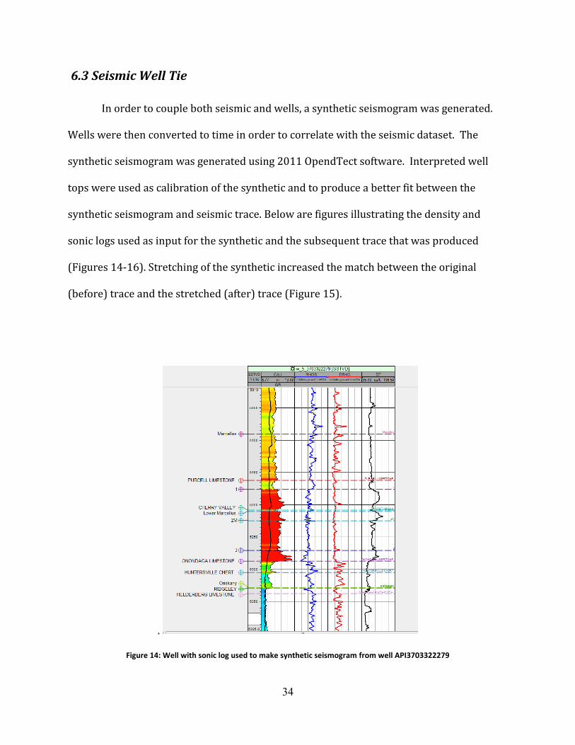
6.3 Seismic Well Tie

In order to couple both seismic and wells, a synthetic seismogram was generated.

Wells were then converted to time in order to correlate with the seismic dataset. The

synthetic seismogram was generated using 2011 OpendTect software. Interpreted well

tops were used as calibration of the synthetic and to produce a better fit between the

synthetic seismogram and seismic trace. Below are figures illustrating the density and

sonic logs used as input for the synthetic and the subsequent trace that was produced

(Figures 14-16). Stretching of the synthetic increased the match between the original

(before) trace and the stretched (after) trace (Figure 15).

.

Figure 14: Well with sonic log used to make synthetic seismogram from well API3703322279

35

Figure 16: Example of well log and seismic data after time depth conversion from synthetic seismogram.

Note surface of Onondaga Limestone match well with well top picks for that formation.

Amount of

offset

Before After

Figure 15: Synthetic seismogram from well API3703322279.

36

7. RESULTS

7.1 Geologic Structure and Stratigraphy Interpretations

Figure 17 depicts the Middle Devonian interval for this study and the associated

horizons. Several surfaces were generated throughout the seismic volume to observe

structural variations with depth. The first three surfaces are of particular importance, as

they are situated within the Middle Devonian interval and include the Tully Limestone,

Marcellus Shale and Onondaga Limestone, respectively. The Tully Limestone has a

distinctive high amplitude trace. As a result, it was used to estimate the horizons for the

underlying Marcellus Shale, Onondaga Limestone, Oriskany Sandstone, and Salina Salt

stratigraphic units. Additional surfaces were picked below the Middle Devonian interval to

observe any lower structures that may have influenced deformation.

From crossline and inline examination, major seismic-scale faults and folds within

the Middle Devonian interval were identified. Stratigraphic units, including the Marcellus

Shale, Onondaga Limestone, and Oriskany Sandstone were structurally more susceptible to

compressional stresses associated with orogenic activity because they overly the Silurian

Salina Salt that is mechanically weak and serves as the primary detachment horizon. As a

result, this interval is deformed significantly more than the layers above and below, leading

to a distinctive detached structural style that contrast strongly with the underlying pre-salt

basement-involved rift-sag basins. Since these structural components have become

increasingly important for unconventional hydrocarbon extraction, it was necessary to

delineate their locations, distribution, connectivity, and orientation within the study area.

37

Figures 18 shows the surface of the Marcellus Shale and the major structural

components influencing the area, with cooler colors representing deeper time structures

and warmer colors representing shallower two-way travel (TWT) time structures.

Observations from the Marcellus surface indicate predominant lows to the west-southwest,

interpreted to be opposite-vergent thrusts (Figure 17). A cross-strike NW-trending

lineament, determined to be a major transfer fault, lays to the north-central region cross-

cutting the regional NE-trending folds and thrusts (Figure 18). This structural high is

observed throughout the Middle Devonian interval and is a major structural component of

the field. Several NE- and NW-trending lineaments are present at both the Marcellus and

Oriskany structural levels (Figure 18).

Although the suggested major transfer fault continues onto the Oriskany surface, the

opposite-vergent thrusts become less evident with depth and it is difficult to discern

whether or not they penetrate the overlying Tully surface. Observations of structure maps

generated from interpreted horizons indicate similar trends, with lows in the southwest

transitioning to highs in the central northeast but eventually less discernible near the

deepest surface (Figures 19-22). Thus, the vertical relief and penetration of both regional

folds and thrust are mostly restricted to the Devonian interval, however, cross-strike

transfer faults continue with depth.

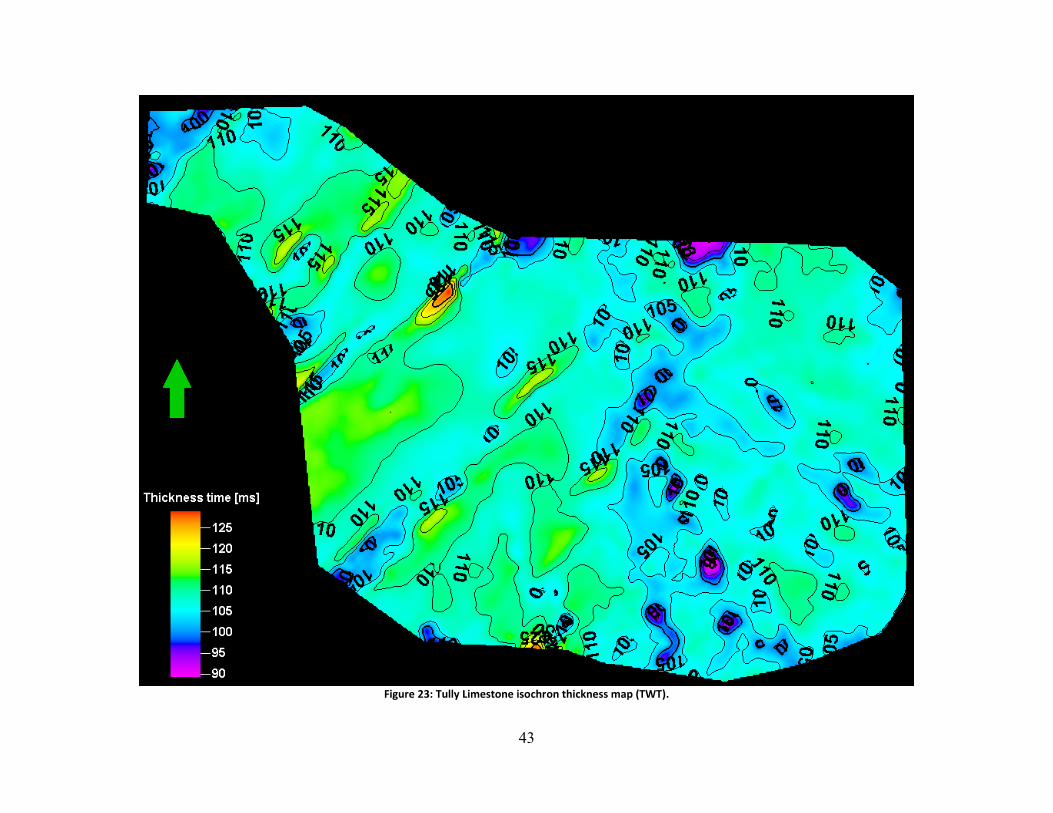
Once surfaces were generated, isopach maps were produced to observe changes in

thickness with depth (Figure 23-26). Little variation was observed in the upper

stratigraphic intervals containing the Marcellus Shale. However, the dominant central

northeast high has greatest thicknesses along the Salina Salt surface, indicating a regional

thickening as a result of movement along the salt detachment surface (Figure 26).

38

Figure 17: Inline 48 showing structure and stratigraphy throughout study area.

Figure 18: Structure map of Onondaga surface with wells (TWT).

NW SE

39

Figure 19: Structure time map of Tully Limestone (TWT).

40

Figure 20: Structure time map of Marcellus Shale (TWT).

41

Figure 21: Structure time map of Oriskany Sandstone (TWT).

42

Figure 22: Structure time map on Salina Salt (TWT).

43

Figure 23: Tully Limestone isochron thickness map (TWT).

44

Figure 24: Marcellus Shale isochron thickness map (TWT).

45

Figure 25: Oriskany Sandstone isochron thickness map (TWT).

46

Figure 26: Salina Salt isochron thickness map (TWT).

47

7.2 Structural Attribute Analysis

Attribute-assisted structural analysis can help to identify fault and fracture

networks that were not easily identified within the raw seismic amplitude data. For

example, through the aid of variance, curvature, and ant tracking, significant breaks in

discontinuity may be highlighted along specific horizons to reveal faults and possible

fracture swarm locations. These observations are important for enhancing hydrocarbon

exploration and gas recovery within the Middle Devonian interval (Figure 17).

The waveform model regression (WMR) attribute was applied to the 3D seismic

volume to better highlight structural features within the dataset. Figures 27-32 show both

along-strike and cross-strike displays throughout the seismic dataset. Discontinuities were

initially interpreted from this attribute, while stepping through the seismic volume.

Cross-strike structural variation using the WMR attribute (Figures 27-30) revealed

high angle reverse faults that were interpreted to detach within the salt interval. Opposite-

verging thrust faults extend throughout the study area and appear to merge together

towards the center of the dataset (Figure 27-30, cross-section A1-A3). Note the bright

marker associated with the Tully Limestone has been significantly displaced along these

high angle reverse faults. Similar structures have been observed from seismic datasets

within Clearfield County have been published (Shultz, 1999).

Along-strike structural variation was also assessed using the waveform model

regression attribute. Numerous high angle faults, interpreted to be fracture damage zones

were mapped. Stepping through the volume from cross-section B1 to B2, a major fault

damage zone begins in the north-central part of the dataset and separates into two damage

zones towards the southeast. Comparisons between cross-sections B1 and B2 in figure 31

48

and 32 best illustrates this change in intensity of deformation throughout the seismic

volume.

The WMR attribute significantly enhances the structure within the 3D seismic

volume by highlighting opposing thrust geometries and flower structures, as well as, near-

vertical faults with a possible strike-slip component. Although major faults were apparent

from regular amplitude data, the WMR attribute appears to highlight structural features

with greater detail. As a result, it was possible to interpret structures that may be related to

faults or fault damage zones (Figures 27-32).

Several near-vertical faults were interpreted to extend throughout Ordovician to

Devonian intervals. Fracture swarms and fault damage zones may surround many of these

major interpreted faults. These zones serve as the greatest risk for well planning and

hydraulic fracture stimulation since they may interconnect and thus communicate with one

another. Moreover, if these fracture swarms are associated with a transpressional, strike-

slip shearing component, an additional amount of risk should be considered since fractures

could have a greater potential for fluid migration as a result of shearing potential and

interconnectivity.

The attribute anomalies discussed in this paper are most readily apparent when

most positive curvature and most extreme curvature values are derived from the seismic

data volume. The red colors indicate positive curvature areas, while blue colors represent

less positive/negative curvature values. These locations highlight areas of most intensive

folding, potentially identifying local bending (anticlinal and synclinal structures) associated

with faulting and fracturing.

49

Three well developed trends are identified in the curvature data for the Middle

Devonian intervals and are shown in Figures 33-40 below. A time slice was observed at

975ms and lies within the Tully Limestone formation (Figure 33 and 37). The curvature

attribute enhances visualization of the ENE trending lineaments, indicated with a red

arrow for orientation. These structures have similar orientations as the J1 set orientation

commonly seen throughout the Marcellus.

Figures 34 and 38 show time slices at 1058ms for the Marcellus Shale interval. In

these time slices, the ENE trending lineaments are still observed but a second set, similar to

the J2 set orientation, is easily discernible with the NNW orientation indicated by a blue

arrow. These regularly occurring ENE and NNW trending linear curvature anomalies are

observed in all horizons throughout the Middle Devonian interval and likely enhance fluid

migration.

Aside from the ENE and NNW trending lineaments, a third set of lineaments striking

to the NW, is observed. Figures 33-40 illustrate these cross-regional lineaments with a

yellow arrow. This trend is believed to represent lineaments which may be the dominant

fluid migration pathways. Near-vertical strike-slip faults could potentially allow

transportation of hydraulic fracturing fluids, thus decreasing efficiency in recovering

hydrocarbons.

Similar observations are observed to continue with increasing depth. Positive

curvature is also observed near the top of the Salina Salt, with several orientations

apparent. This chaotic pattern may likely associate with movement along the Silurian

Salina Salt detachment surface and to some degree influenced by increases in seismic noise

(Figure 36 and 40).

50

Two additional attributes (variance and ant tracking) were applied for the

enhancement of discontinuities within the dataset. The variance attributes is useful for

edge detection because it represents the trace-to-trace variability of amplitude. Areas of

high variance are shaded with warmer colors (red-yellow), whereas areas of low variance

are shaded in gray with whites having the least variation among neighboring wiggle traces

(Figures 41-44).

Variance values obtained from the seismic amplitude volume are viewed at the

same horizons as the curvature attribute. Similar trends were identified with those detailed

in the curvature attribute analysis, although J2 set orientations, trending NNW (indicated

by blue arrow) and cross regional NW lineament (indicated by yellow arrow) were

somewhat difficult to discern (Figure 41-42) but the regularly occurring ENE trending

lineaments were apparent throughout the Marcellus and Oriskany surfaces (Figure 42-43,

indicated by red arrow). Below the Middle Devonian interval, variance anomalies were

minimal.

One notable difference was observed when viewing surfaces near the Tully

Limestone with the variance attribute, that was not obvious from the curvature attribute

alone. The NNW-trending lineaments (indicated by blue arrow) and cross-strike NW-

lineaments (indicated by yellow arrow) are still observed; however, ENE-trending faults

(indicated by red arrow) were not seen to penetrate the Tully surface (Figure 41). This may

prove to be of great importance, since the vertical extent of these faults above the Tully

Limestone could be detrimental to hydraulic stimulation if fluids were to travel above this

depth.

51

The ant tracking attribute was applied to the variance volume for better edge

enhancement. Then ant tracking was recomputed using the new volume generated from

the ant tracking on variance, to further enhance visualization. Again, regularly occurring

ENE, NNW and cross-strike NW trending lineaments were observed. Figures 45-50 show

the results of this seismic attribute, with the respective colored arrows representing the

three lineament trends.

From the ant-tracking attribute, a possible transpressional strike-slip shearing style

may be expressed in the Middle Devonian interval near the Marcellus Shale formation

(Figure 45-50). The dominant WNW-trending lineament to the north was not identified in

either the curvature or variance attribute (Figure 46). This lineament is thought to be

below seismic resolution. Since there was a component of shortening during the time of

deformation for these intervals, oblique shearing could have occurred. This particular fault

(indicated by yellow arrow orientation) appears to directly connect to the main NW-

trending lineament, further complicating the structural complexity of the area. In the event

that this shear fault exists, it would prove to have great influence on hydraulic fluid

transportation and gas recovery. Open-mode fractures and faults associated with this

particular style may act as fluid migration pathways, thus hindering gas recovery in the

area of interest.

Comparison of structures observed from the WMR attribute compared to seismic

attribute maps (time slice) from curvature, variance, and ant tracking have a good

correlation. Areas with greater fracture intensity observed in cross-sectional view matched

with areas of greatest curvature and variance. A structural feature located in the south-

central portion of the study area was not easily discernible from regular amplitude data.

52

However, the WMR attribute showed near vertical faults in this area which were in

agreement with attribute maps (Figure 31-32).

Two ages of faulting were observed from vertical observations of the seismic data.

Faults trending to the northeast are likely associated with the Acadian Orogeny which

occurred between the Middle Devonian to Early Mississippian. This orogeny was the result

of the micro-continent of Avalon colliding with the eastern margin of Laurentia. As a result,

extension in the Allegheny Plateau region mobilized the Silurian Salina Salt (Shultz, 1999).

Northeastern trending faults in the dataset extend only to the uppermost Middle Devonian

interval and terminate along the Salina Salt detachment, making their age congruent with

that of the Acadian Orogeny.

Faults trending to the northwest are likely associated with the Allegheny Orogeny.

This orogeny occurred from the Late Mississippian to Early Permian in which complex

deformation resulted from the collision of Gondwana and the Peri-Gondwana continents

(Shultz, 1999). Several northwest trending faults in the dataset extend well above the

Mississippian interval and into the stratigraphic members of Permian age. Thus, northwest

trending faults are consistent with the timing of deformation during the Allegheny

Orogeny.

53

B2

B1

A1 A2 A3

Figure 27: Above: WMR attribute showing time slice through the Marcellus Shale and Onondaga Limestone intervals with along strike and cross-strike cross-sections. Right: Uninterpreted inline A1 showing Middle Devonian structure. The WMR attribute significantly enhanced the structure within the 3D seismic volume by highlighting opposing

thrust geometries associated with compressional stresses.

A1

Tully Ls. Marcellus Sh. Onodaga Ls. Oriskany Ss. Salina Salt

54

B2

B1

A1 A2 A3

Figure 28: Above: WMR attribute showing time slice through the Marcellus Shale and Onondaga Limestone intervals with along strike and cross-strike cross-sections. Right: Interpreted inline A1 showing Middle Devonian structure. The WMR attribute significantly enhanced the structure within the 3D seismic volume by highlighting opposing

thrust geometries associated with compressional stresses. Interpreted faulting is highlighted by red lines.

A1 Tully Ls. Marcellus Sh. Onodaga Ls. Oriskany Ss. Salina Salt

55

Figure 29: Uninterpreted inlines A2 and A3 showing Middle Devonian structure. The WMR attribute significantly

enhanced the structure within the 3D seismic volume by highlighting opposing thrust geometries associated with compressional stresses.

A2

A3

Tully Ls. Marcellus Sh. Onodaga Ls. Oriskany Ss. Salina Salt

Tully Ls. Marcellus Sh. Onodaga Ls. Oriskany Ss. Salina Salt

56

A3

A2

Figure 30: Interpreted inlines A2 and A3 showing Middle Devonian structure. The WMR attribute significantly enhanced the structure within the 3D seismic volume by highlighting opposing thrust geometries associated with compressional stresses. Interpreted faulting is highlighted by red lines. Solid lines indicate apparent faults while

dashed lines indicate ambiguous features that may represent faults or fault damage zones.

Tully Ls. Marcellus Sh. Onodaga Ls. Oriskany Ss. Salina Salt

Tully Ls. Marcellus Sh. Onodaga Ls. Oriskany Ss. Salina Salt

57

A1

B2

B2

B1

A1 A2

A3

Figure 31: WMR attribute showing time slice through the Marcellus Shale and Onondaga Limestone intervals with along strike and cross-strike cross-sections. Right: Uninterpreted crosslines B1 and B2 showing Middle Devonian structure. The WMR attribute significantly enhanced the structure within the 3D seismic volume by highlighting opposing thrust geometries, potential flower structures and near-vertical faults with a possible strike-slip component.

B1 Tully Ls. Marcellus Sh. Onodaga Ls. Oriskany Ss. Salina Salt

Tully Ls. Marcellus Sh. Onodaga Ls. Oriskany Ss. Salina Salt

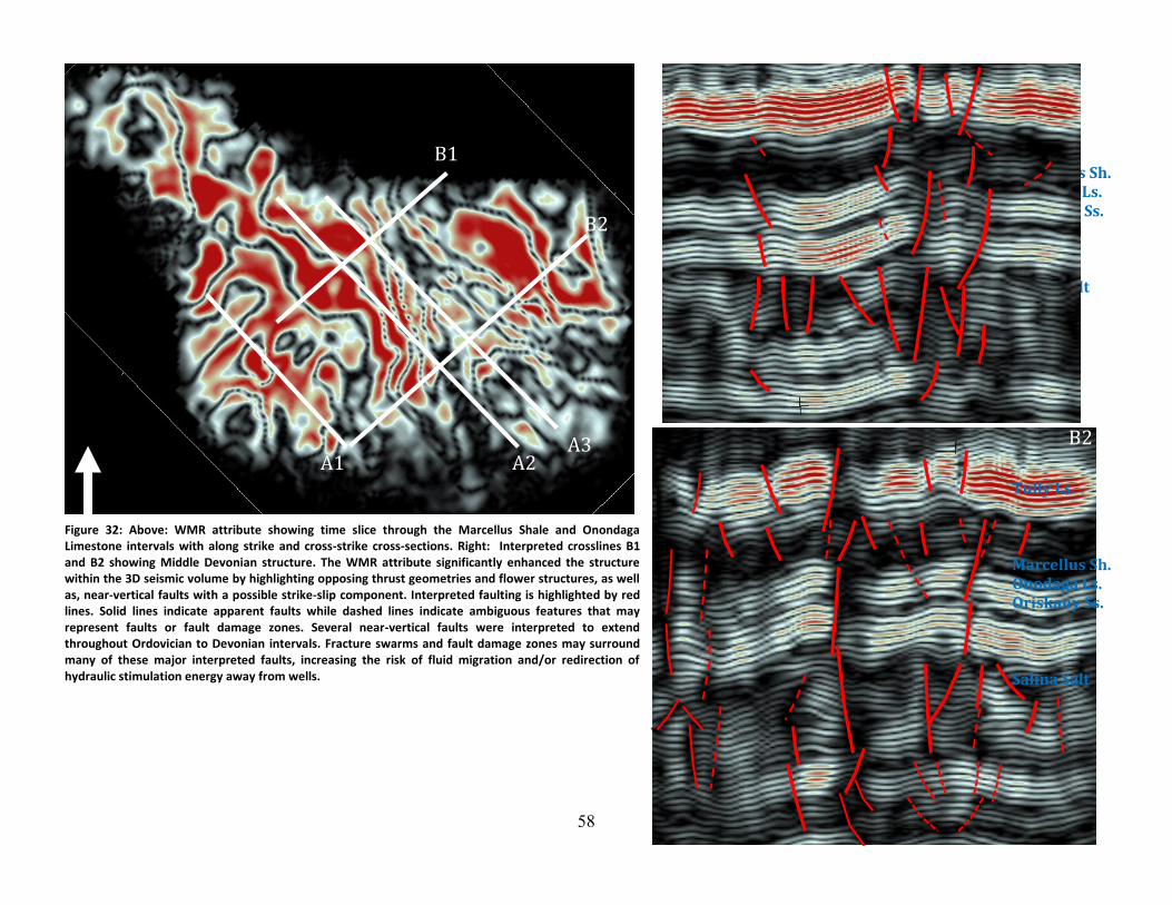
58

A1 A1

B2

B1

A1 A2 A3

Figure 32: Above: WMR attribute showing time slice through the Marcellus Shale and Onondaga Limestone intervals with along strike and cross-strike cross-sections. Right: Interpreted crosslines B1 and B2 showing Middle Devonian structure. The WMR attribute significantly enhanced the structure within the 3D seismic volume by highlighting opposing thrust geometries and flower structures, as well as, near-vertical faults with a possible strike-slip component. Interpreted faulting is highlighted by red lines. Solid lines indicate apparent faults while dashed lines indicate ambiguous features that may represent faults or fault damage zones. Several near-vertical faults were interpreted to extend throughout Ordovician to Devonian intervals. Fracture swarms and fault damage zones may surround many of these major interpreted faults, increasing the risk of fluid migration and/or redirection of hydraulic stimulation energy away from wells.

A1

B1

B2

Tully Ls. Marcellus Sh. Onodaga Ls. Oriskany Ss. Salina Salt

Tully Ls. Marcellus Sh. Onodaga Ls. Oriskany Ss. Salina Salt

B1

59

Figure 33: Curvature attribute for time slice (~975ms) of the Tully Limestone. Note prominent NNW striking lineaments, similar to the J2 set orientations commonly

observed in the Middle Devonian interval.

60

Figure 34: Curvature attribute for time slice (~1058ms) of the Marcellus Shale. Note ENE striking lineaments, similar to the J1 set orientations commonly observed in the

Middle Devonian interval.

61

Figure 35: Curvature attribute for time slice (~1080ms) near the Oriskany Sandstone. Note ENE striking lineaments, similar to the J1 set orientations commonly observed in

the Middle Devonian interval.

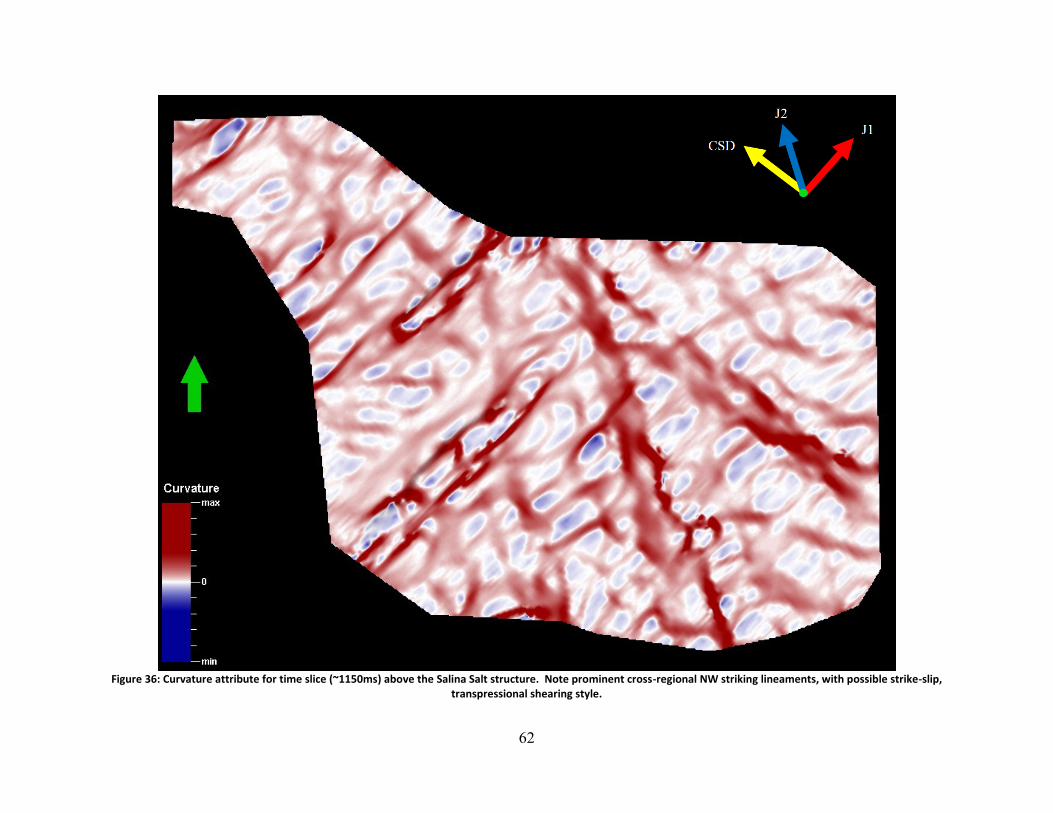
62

Figure 36: Curvature attribute for time slice (~1150ms) above the Salina Salt structure. Note prominent cross-regional NW striking lineaments, with possible strike-slip,

transpressional shearing style.

63

Figure 37: Most extreme curvature attribute for time slice (~975ms) of the Tully Limestone. Note prominent NNW striking lineaments, similar to J2 set orientations

commonly observed in the Middle Devonian interval.

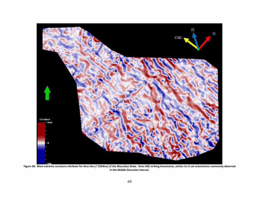
64

Figure 38: Most extreme curvature attribute for time slice (~1058ms) of the Marcellus Shale. Note ENE striking lineaments, similar to J1 set orientations commonly observed

in the Middle Devonian interval.

65

Figure 39: Most extreme curvature attribute for time slice (~1080ms) near the Oriskany Sandstone. Note ENE striking lineaments, similar to J1 set orientations commonly

observed in the Middle Devonian interval.

66

Figure 40: Most extreme curvature attribute for time slice (~1150ms) above the Salina Salt structure. Note prominent cross-regional NW striking lineaments, with possible

strike-slip, transpressional shearing style.

67

Figure 41: Variance attribute for time slice (~974ms) of the Tully Limestone. Note prominent NNW striking lineaments (yellow arrow), similar to the J2 set orientations

commonly observed in the Middle Devonian interval.

68

Figure 42: Variance attribute for time slice (~1058ms) near the Marcellus Shale. Note ENE striking lineaments (red arrow), similar to the J1 set orientations commonly

observed in the Middle Devonian interval. Possible cross-regional NW striking lineaments (blue arrow).

69

Figure 43: Variance attribute for time slice (~1080ms) near the Oriskany Sandstone. Note ENE striking lineaments (red arrow), similar to the J1 set orientations commonly

observed in the Middle Devonian interval. Possible cross-regional NW striking lineaments (blue arrow).

70

Figure 44: Variance attribute for time slice (~1150ms) above the Salina Salt structure.

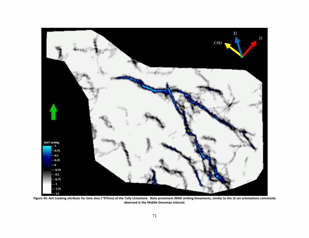
71

Figure 45: Ant tracking attribute for time slice (~975ms) of the Tully Limestone. Note prominent NNW striking lineaments, similar to the J2 set orientations commonly

observed in the Middle Devonian interval.

72

Figure 46: Ant tracking attribute for time slice (~1058ms) of the Marcellus Shale. Note ENE striking lineaments, similar to the J1 set orientations commonly observed in the

Middle Devonian interval. Possible cross-regional NW striking lineaments indicative of transpressional strike slip shearing style.

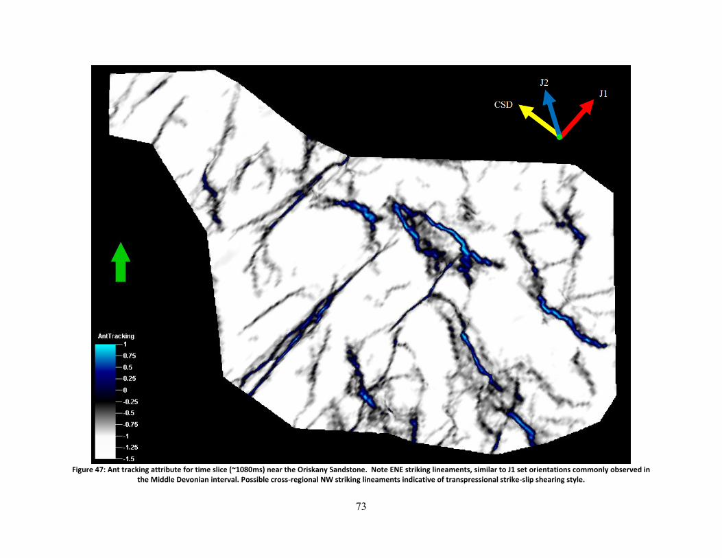
73

Figure 47: Ant tracking attribute for time slice (~1080ms) near the Oriskany Sandstone. Note ENE striking lineaments, similar to J1 set orientations commonly observed in

the Middle Devonian interval. Possible cross-regional NW striking lineaments indicative of transpressional strike-slip shearing style.

74

Figure 48: Ant tracking attribute for time slice (~1150ms) above the Salina Salt structure.

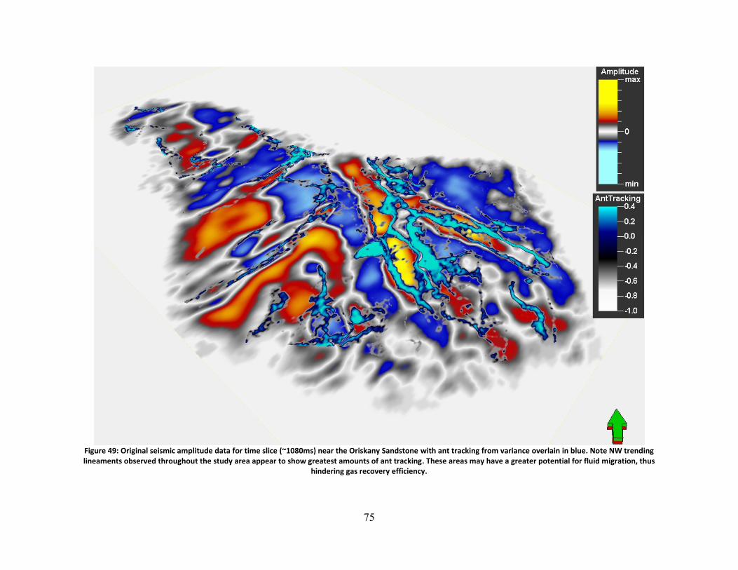
75

Figure 49: Original seismic amplitude data for time slice (~1080ms) near the Oriskany Sandstone with ant tracking from variance overlain in blue. Note NW trending lineaments observed throughout the study area appear to show greatest amounts of ant tracking. These areas may have a greater potential for fluid migration, thus

hindering gas recovery efficiency.

76

Figure 50: Variance attribute data for time slice (~1080ms) near the Oriskany Sandstone with ant tracking from variance overlain in blue. Note NW trending lineaments observed throughout the study area appear to show greatest amounts of ant tracking. These areas may have a greater potential for fluid migration, thus hindering gas

recovery efficiency.

77

7.3 Correlation of Seismic Data with FMI Log Data

One well, located approximately 2 miles outside of the 3D seismic dataset, contained

a formation microimager (FMI) log. This type of log determines real-time resistivity

measurements by emitting a current throughout the rock adjacent to the borehole

(Schlumberger, 2013). This logging tool is especially useful for fault and fracture analysis,

as it generates a 360 degree resistivity image of the wellbore. This allows the interpreter to

identify faults and fracture locations, dip, and azimuth. Since an FMI log was available and

near the dataset, an opportunity to compare orientations and dips determined from the

FMI log with fault orientations and dips determined by Petrel’s 2012 automatic fault

extraction process was possible.

Figures 51 through 55 show the FMI log data and automatic faults extracted from

Petrel 2012 (from ant tracking volume with variance as input) with their associated

orientation and dip interpretations, respectively. Both datasets exhibit two primary

orientations: northeast-southwest and northwest-southeast. Similar trends were observed

through seismic attribute analysis of the 3D seismic dataset.

78

Figure 51: Formation Microimager log from a well outside of the 3D seismic dataset, with interpreted fractures shown.

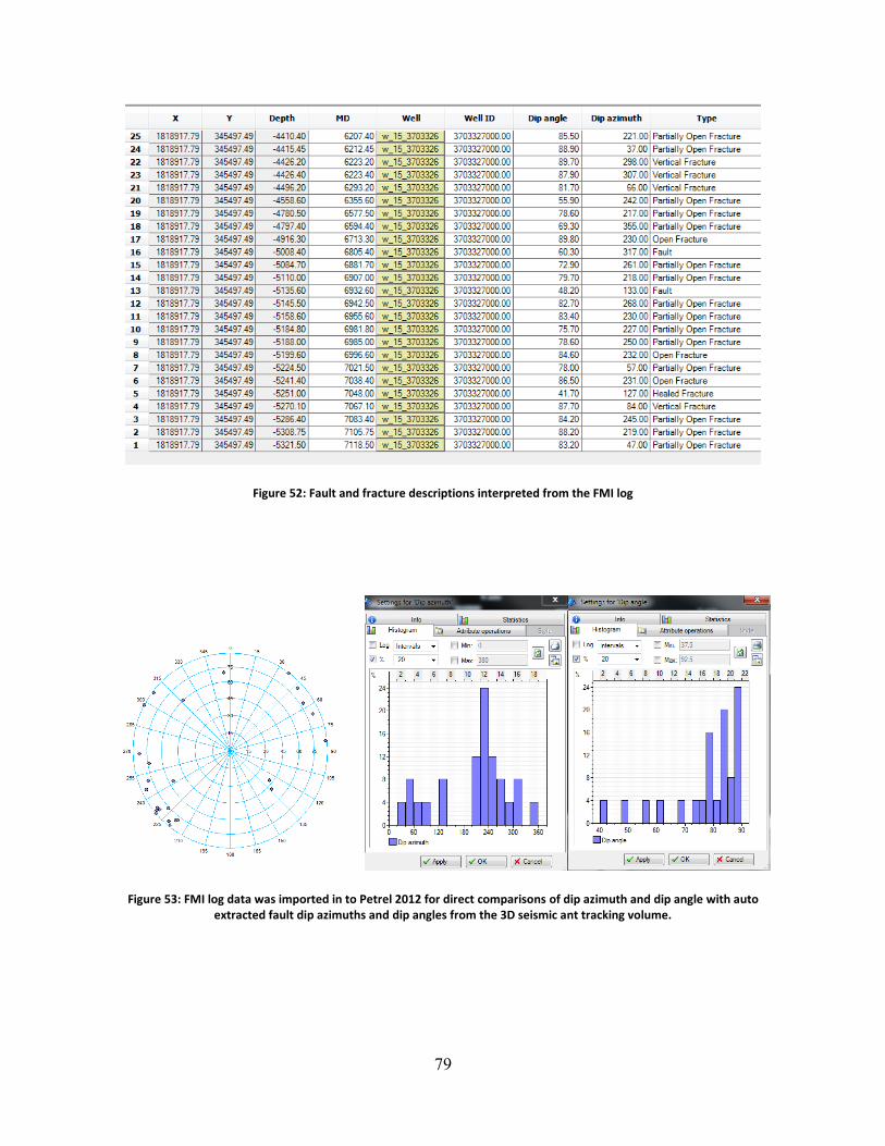
79

Figure 52: Fault and fracture descriptions interpreted from the FMI log

Figure 53: FMI log data was imported in to Petrel 2012 for direct comparisons of dip azimuth and dip angle with auto extracted fault dip azimuths and dip angles from the 3D seismic ant tracking volume.

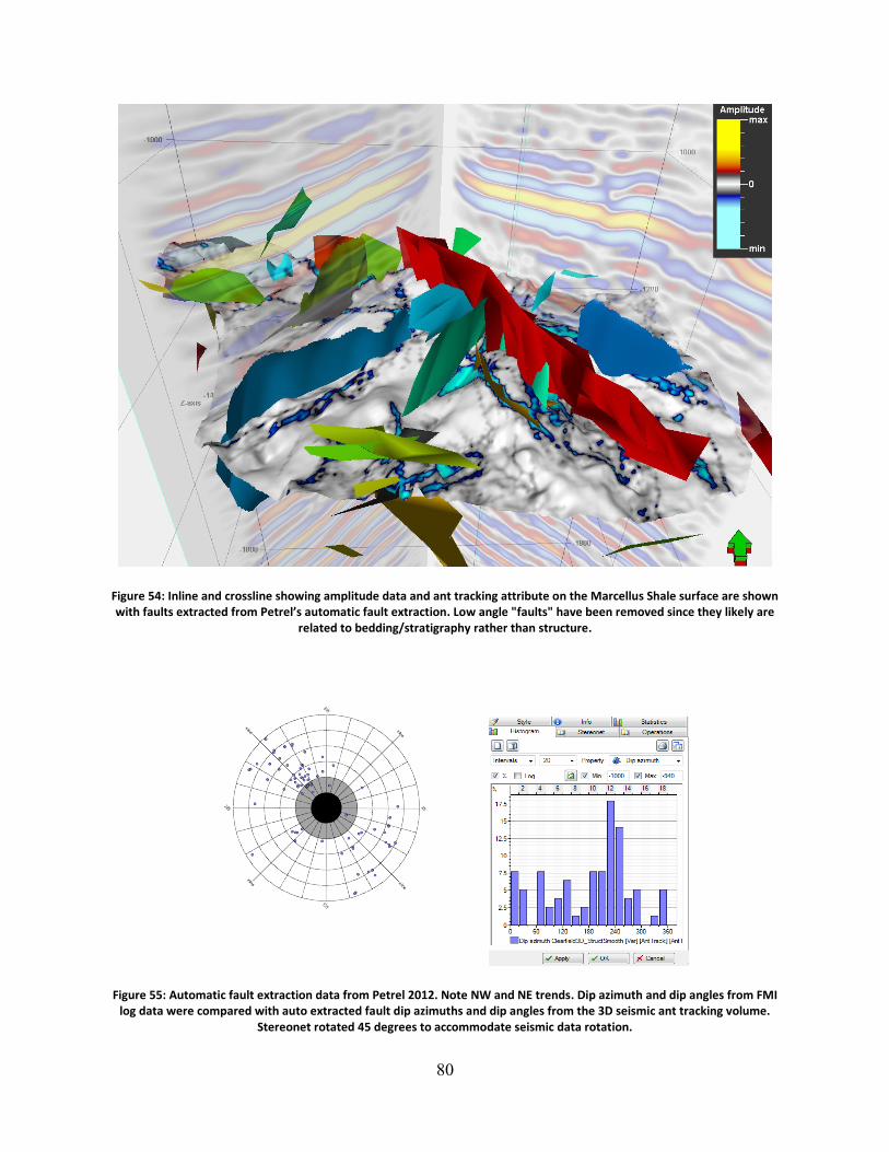
80

Figure 54: Inline and crossline showing amplitude data and ant tracking attribute on the Marcellus Shale surface are shown with faults extracted from Petrel’s automatic fault extraction. Low angle "faults" have been removed since they likely are

related to bedding/stratigraphy rather than structure.

Figure 55: Automatic fault extraction data from Petrel 2012. Note NW and NE trends. Dip azimuth and dip angles from FMI log data were compared with auto extracted fault dip azimuths and dip angles from the 3D seismic ant tracking volume.

Stereonet rotated 45 degrees to accommodate seismic data rotation.

81

7.4 Correlation of Seismic Data with Surface Fracture Orientations and Breakout Data

In the Appalachian basin, numerous faults and fractures have been mapped along

the surface (Bruner and Smosna, 2011; Durham, 2011; Lash and Engelder, 2011; Engelder

et al., 2009). As discussed in chapter 2, several joint sets have been mapped. From these

joint sets, tectonic paleo-stresses are inferred. Additional data, such as those shown in

figure 56 are used to determine present-day stress relationships.

Three dominant trends were observed throughout this 3D seismic dataset and

include: 1.) NE-SW trending lineaments, which is possibly related to the previously

reported J1 set orientation, and 2.) NNW-SSE trending and NW-SE trending lineaments,

both of which are suggested to be related to the regular J2 set orientations commonly seen

throughout the basin (Bruner and Smosna, 2011; Engelder et al., 2009). These three

dominant trends correlate well with orientations from regional borehole breakout data,

earthquake focal mechanism data and hydraulic fracture data observed in this area of the

basin (Figure 56).

These findings are significant for fault and fracture interpretations of the subsurface

through the use of seismic attribute analysis. A strong correlation between fault and

fracture orientations on the local and regional scale is clearly evident. Thus, a greater

amount of confidence in the interpretation of these structural discontinuities can be taken

as it provides a realistic representation of structures in the subsurface.

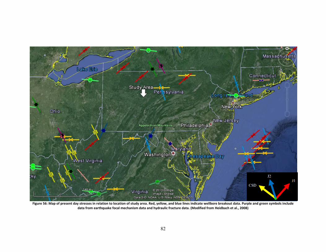
82

Figure 56: Map of present day stresses in relation to location of study area. Red, yellow, and blue lines indicate wellbore breakout data. Purple and green symbols include

data from earthquake focal mechanism data and hydraulic fracture data. (Modified from Heidbach et al., 2008)

83

8. CONCLUSIONS

3D seismic analysis is a useful application for both conventional and unconventional

reservoir exploration. Seismic data can provide valuable information over a large area that

may not be easily observed from petrophysical analysis and well log correlation alone. The

analysis of seismic attributes helps to better understand the structural and stratigraphic

complexities in the subsurface that would typically fall below the resolution of traditional

seismic amplitude data. Attributes examined in this study consist of curvature, variance,

and ant tracking, but there is potential for applications of other attributes, such as spectral

decomposition (Partyka, Gridley, and Lopez 1999 and wavelet spectral probing (Gao,

2013).

Three regularly occurring structural lineaments have been identified and mapped

within the Middle Devonian interval. These include ENE-trending lineaments at

approximately 50-60 degrees, NW-trending lineaments at approximately 315-345 degrees

and a third possible NW-trending lineament set. This third set may have a more

transpressional shearing component than the second one due to their orientation relative

to the compressional stress σ 1. If these fractures are determined to be open natural

fractures, they may intersect permeable and porous formations above or below the

reservoir, and potentially cause the loss of injection fluids by means of absorption and/or

redirection of energy along specific fault and fractures.

The ENE trending faults may be associated with the regular J1 set orientations

commonly observed throughout the basin, thus enhancing production (Bruner and Smosna,

2011; Lash and Engelder, 2011; Durham, 2011; Engelder et al., 2009). These structures are

84

associated with forethrust and backthrust structures along the major Salina Salt

detachment. The ENE trending faults did not appear to penetrate the upper Tully

Limestone horizon. This may prove to be of great importance, since the vertical extent of

these faults above the Tully Limestone could be detrimental to hydraulic stimulation if

fluids were to travel above this depth. If the Tully Limestone in this study area can

effectively act as a fracture barrier, enhanced hydrocarbon recovery may be expected.

The NNW trending lineaments identified in the 3D seismic dataset are most

apparent. This trend appears to correlate with the regular J2 fracture set orientation

commonly observed throughout the basin and thus may enhance production (Bruner and

Smosna, 2011; Lash and Engelder, 2011; Durham, 2011; Engelder et al., 2009). A major

fault to the north-central part of the study area is oriented in this NNW direction. However,

this fault is suggested to be made up of several interconnected vertical fractures which

could potentially hinder gas recovery by redirecting stimulation energy away from wells. A

slightly different fracture set, striking to the NW, is thought to represent lineaments which

may be the dominant fluid migration pathways since these near-vertical strike-slip faults

could potentially allow transportation of hydraulic fracturing fluids, thus decreasing

efficiency in recovering hydrocarbons.

Along-strike structural variation was also assessed using the waveform model

regression attribute. The WMR attribute significantly enhances the structure within the 3D

seismic volume by highlighting opposing thrust geometries and flower structures, as well

as, near-vertical faults with a possible strike-slip component. Numerous high-angle faults

are interpreted to be surrounded by fracture damage zones. A major fault damage zone

85

begins in the north-central part of the dataset and separates into two damage zones

towards the southeast.

Although some major faults were apparent from regular amplitude data, the WMR

attribute appears to highlight structural features with greater detail. As a result, it was

possible to interpret structures that may be related to faults or fault damage zones. In

particular, comparison of structures observed from the WMR attribute compared to

seismic attribute maps (time slice) from curvature, variance, and ant tracking have a good

correlation. Areas with greater fracture intensity observed in cross-sectional view matched

with areas of greatest curvature and variance.

A structural feature located in the south-central portion of the study area was not

easily discernible from regular amplitude data. However, the WMR attribute showed near

vertical faults in this area which were in agreement with attribute maps from curvature,

variance, and ant tracking. These zones serve as the greatest risk for well planning and

hydraulic fracture stimulation since they may interconnect and thus communicate with one

another. Moreover, if these fracture swarms are associated with a transpressional, strike-

slip shearing component, an additional amount of risk should be considered since fractures

could have a greater potential for fluid migration as a result of shearing potential and

interconnectivity.

Through the integration of well logs and 3D seismic data, useful information on the

relationship between structural (faults/fractures/folds), stratigraphic (well log analyses of

depositional facies) and reservoir properties may provide valuable insight for hydrocarbon

extraction and well design. These observations may potentially aid in the enhancement of

86

hydrocarbon extraction within the area and prevent hydraulic fluid migration from faults

which may act as fluid conduits.

Since a formation microimager (FMI) log was readily available and near the dataset,

an opportunity to compare orientations and dips determined from the FMI log with fault

orientations and dips determined by Petrel’s 2012 automatic fault extraction process was

possible. One well, located approximately 2 miles outside of the 3D seismic dataset,

contained an FMI log. This logging tool is especially useful for fault and fracture analysis, as

it generates a 360 degree resistivity image of the wellbore allowing the interpreter to

identify faults and fracture locations, dip, and azimuth.

The three dominant trends were not only observed throughout the Clearfield

County seismic dataset, but are also the same orientations as that of regional borehole

breakout data and earthquake focal mechanism data and hydraulic fracture data. These

findings are significant for fault and fracture interpretations of the subsurface through the

use of seismic attribute analysis. A strong correlation between fault and fracture

orientations on the local and regional scale is clearly evident. Thus, a greater amount of

confidence in the interpretation of these structural discontinuities can be taken as it

provides a realistic representation of structures in the subsurface.

The structural style and intensity, particularly those related to the cross-regional

lineaments, contrast strongly with those in other portions across the Appalachian basin.

Such basin-wide contrast indicates along-axis structural variation and segmentation caused

by the cross-regional transfer faults (Gao et al., 2000) associated with basement-involved

rifting and subsequent post-salt detachment folding and thrusting. Such along-axis

structure variation and segmentation associated with the cross-regional transfer faults

87

have been commonly observed and widely published in rift and foreland basins and

passive margin settings (e.g. Steel, 1988; Van der Pluijm, 2004, Konstantopoulos and

Maravelis, 2013; Gao, 2012a, 2012b, 2013) around the world; whereas their economic and

environmental implications in both conventional and unconventional hydrocarbon

exploration and production remain to be further investigated.

88

9. REFERENCES

Anderson, E.M., 1951, The Dynamics of Faulting: Edinburgh, Oliver, and Boyd, London, p. 214.

Babarsky, A., 2012, 3D seismic attribute-assisted fracture detection in the Middle Devonian Marcellus Shale. Greene and Washington Counties, PA, Central Appalachian Basin: Master’s Thesis, Morgantown, West Virginia University. Babarsky, A., and Gao, D., 2012, 3D seismic attribute-assisted fracture detection in the Middle Devonian Marcellus Shale, southwestern PA, Central Appalachian Basin: SEG Expanded Abstracts, Annual Meeting, Las Vegas, NV, 2012. Bentley, C., 2013, Mountain Beltway: Geologic thoughts from Washington, D.C.: Transect debrief 5: sedimentation continues. Modified from Marshak, S., 2010, Earth: Portrait of a Planet. Retrieved on August, 24, 2013 from http://mountainbeltway.wordpress.com/ category/plate-tectonics. Blakey, R.C., 2008, Gondwana paleogeography from assembly to breakup—A 500 m. y. odyssey, in Fielding, C.R., Frank, T.D., and Isbell, J.L., eds., Resolving the Late Paleozoic Ice Age in Time and Space: Geological Society of America Special Paper 441, p. 1-28, doi: 10.1130/2008.2441(01). Bott, M.H.P., 1959, The mechanics of oblique slip faulting: Geological Magazine, v. 96, No. 2, p. 109-117. Boyce, M. L., 2010, Sub-surface stratigraphy and petrophysical analysis of the Middle Devonian interval of the central Appalachian Basin; West Virginia and Southwest Pennsylvania: Doctoral Dissertation, Morgantown, West Virginia University. Brown, A.R., 1996, Seismic attributes and their classification: The Leading Edge, Society of Exploration Geophysicists, October, p. 1090. Brown, A.R., 2001, Understanding seismic attributes: Geophysics, v. 66, No. 1, p. 47-48. Brown, A.R., 2004, Interpretation of Three-Dimensional Seismic Data: American Association of Petroleum Geologists, AAPG Memoir 42, Investigations in Geophysics, No. 9, p. 541. Bruner, K. R. and Smosna R., 2011, A Comparative Study of the Mississippian Barnett Shale, Fort Worth Basin, and Devonian Marcellus Shale, Appalachian Basin. Retrieved on December 22, 2011 from: http://www.netl.doe.gov/technologies/oil-gas/publications/brochures/DOE-NETL-2011-1478%20Marcellus-Barnett.pdf

89

Chopra S. and Marfurt K. J., 2007, Seismic Attributes for Prospect ID and Reservoir Characterization. Society of Exploration Geophysicists, ISBN 1-56080-141-7. Cooke, M.L. and Underwood, C.A., 2000, Fracture termination and step-over at bedding interfaces due to frictional slip and interface opening: Journal of Structural Geology, v. 23, p. 223-238. Donahoe, T., 2011, 3D seismic attribute-assisted subsurface interpretation in central Appalachian Basin: Master’s Thesis, Morgantown, West Virginia University.

Donahoe, T., and Gao, D., 2012, Application of 3D seismic attribute analysis to subsurface structure interpretation and hydrocarbon exploration: Southwest Pennsylvania, Central Appalachian Basin. SEG Expanded Abstracts, Annual Meeting, Las Vegas, NV, 2012.

Durham, L.S., 2011, Exploration Approaches Affected: Marcellus Core Areas Differentiated. Retrieved on December 22, 2011 from: http://www.Durham.org/explorer /2011/05may/mar_update0511.cfm. Edmonds, C. A., 2004, Natural gas exploration associated with fracture systems in Alleghenian thrust faults in the Greenbrier Formation, southern West Virginia: Master’s Thesis, West Virginia University. Engelder, T., Lash, G. G., and Uzcategui, R.S., 2009, Joint sets that enhance production from Middle and Upper Devonian gas shales of the Appalachian Basin. Association of Petroleum Geologists Bulletin, v. 93, No. 7, p. 857-889.

Gao, D., 2002, Seismic textures aid exploration, Offshore, v. 62, No.9, p. 65.

Gao, D., 2004, Texture model regression for effective feature discrimination: Application to seismic facies visualization and interpretation, Geophysics, v. 69, p. 958-967. Gao, D., 2011, Latest developments in seismic texture analysis for subsurface structure, facies, and reservoir characterization: A review, Geophysics, v. 76, p. W1-W13. Gao, D., 2012a, Dynamic interplay among tectonics, sedimentation, and petroleum systems: An introduction and overview, in D. Gao, ed., Tectonics and Sedimentation: Implications for petroleum systems: AAPG Memoir 100, p. 1-14. Gao, D., 2013, Wavelet spectral probe for seismic structure interpretation and fracture characterization: A workflow with case studies, Geophysics, v.78, p. O57–O67. Gao, D., and Milliken, J., 2012b, Cross-regional intraslope lineaments on the Lower Congo Basin Slope, offshore Angola (west Africa): Implications for tectonics and petroleum systems at passive continental margins, in D. Gao, ed., Tectonics and sedimentation: Implications for petroleum systems, AAPG Memoir 100, p. 229-248.

90

Gao, D. and Shumaker, R.C., 1996, Subsurface geology of the Warfield structures in southwestern West Virginia: Implications for tectonic deformation and hydrocarbon exploration in the central Appalachian basin, AAPG Bulletin, v. 80, p.1242-1261. Gao, D. and Shumaker, R. C., and Wilson, T.H., 2000, Along-axis segmentation and growth history of the Rome trough: Central Appalachian Basin, AAPG Bulletin, v. 84, p. 75-99. Hart, B.S., Pearson, R., Rawling, G.C., 2002, 3-D seismic horizon-based approaches to fracture-swarm sweet spot definition in tight-gas reservoirs, The Leading Edge, Society of Exploration Geophysicists, January, p. 28-35. Heidbach, O., Tingay, M., Barth, A., Reinecker, J., Kurfeß, D., and Müller, B., 2008, The World Stress Map database release 2008, doi:10.1594/GFZ.WSM.Rel2008, 2008. Hibbard, J., 2004, The Appalachian Orogen, in van der Pluijm, B. and Marshak, S., 2nd edition, Earth Structure: An Introduction to Structural Geology and Tectonics, WCB/McGraw Hill, p. 582-592. Hsieh, P.A. and others, 1993, Methods of characterizing fluid movement and chemical transport in fractured rock: in Cheyney, J.T., Hepburn, C.J., eds., Field Trip Guidebook for the Northeastern United States, Geological Society of America Field Trip Guidebook, Boston GSA, p. 30. King, H.M., nd., Marcellus Shale-Appalachian Basin Natural Gas Play. Retrieved on December 22, 2011 from http://geology.com/articles/marcellus-shale.shtml. Konstantopoulos, P. A., Maravelis, A. G., 2013, The implication of transfer faults in foreland basin evolution: application on Pindos foreland basin, West Peloponnesus, Greece. Terra Nova, v. 25, No. 4, p. 323-336. DOI: 10.1111/ter.12039.

Kulander, B.R., and Dean, S. L., 1980, Rome trough relationship to fracture domains, regional stress history and decollement structures: western limits of detachment and related structures in the Appalachian foreland: U.S. Department of Energy, Morgantown Energy Technology Center, DOE/METC/SP-80/23, p.64-81. Kulander, B. R., and Dean, S. L., 1986, Structure and tectonics of central and southern Appalachian Valley and Ridge and Plateau Provinces, West Virginia and Virginia. American Association of Petroleum Geologists Bulletin, v. 70, No. 11, 1674-1684. Kulander, C. S., and Ryder, R. T., 2005, Regional seismic lines across the Rome Trough and Allegheny Plateau of northern West Virginia, western Maryland, and southwestern Pennsylvania. U.S. Geological Survey, Geologic Investigations Series, I-2791. Lash, G.G., and Engelder, T., 2011, Thickness trends and sequence stratigraphy of the Middle Devonian Marcellus Formation, Appalachian Basin: Implications for Acadian

91

foreland basin evolution, American Association of Petroleum Geologists Bulletin, v. 95, No. 1, p. 61-103. Milici, Robert C. and Swezey, Christopher S., 2006, Assessment of Appalachian Basin Oil and Gas Resources: Devonian Shale—Middle and Upper Paleozoic Total Petroleum System, United States Geological Survey: Open-File Report Series 2006-1237. Olson, J.E., 2004, Predicting fracture swarms; the influence of subcritical crack growth and the crack-tip process zone on joint spacing in rock: in Cosgrove, J.W. and Engelder, T., eds., The initiation, propagation, and arrest of joints and other fractures, Geological Society Special Publications, Geological society of London, v. 231, p. 73-88. Partyka, G. A., Gridley, J. M., and Lopez, J., 1999, Interpretational Applications of Spectral Decomposition in Reservoir Characterization, The Leading Edge, Society of Exploration Geophysicists, v. 18, No. 3, p. 353-360. Shumaker, R. C. and Wilson, T. H., 1996, Basement structure of the Appalachian foreland in West Virginia: Its style and effect on sedimentation, GSA Special Papers 308, p. 139-155. Schlumberger, 2013, Schlumberger Oilfield Glossary: Seismic attributes. Retrieved on July 12, 2013 from http://www.glossary.oilfield.slb.com/en/Terms.aspx?LookIn=term%20 nameandfilter=attribute. Shultz, C.H., 1999, The Geology of Pennsylvania, Pennsylvania Geological Survey and Pittsburgh Geological Society: Harrisburg, Pennsylvania. Shipton, Z. K. and Cowie, P. A., 2003, A conceptual model for the origin of fault damage zone structures in high-porosity sandstone, Journal of Structural Geology, v. 25, p. 333-345.

Stearns, D.W. and Friedman, M., 1972, Reservoirs in fractured rock: in King, R.E., ed., Stratigraphic oil and gas fields; Classification, Exploration Methods, and Case Studies, American Association of Petroleum Geologists Memoir, v. 16, No. 10, p. 82-106. Taner, MT., 2001, Seismic attributes: Canadian Society of Exploration Geophysicists Recorder, September, p. 48-56.

Steel, R. J., 1988, Coarsening-upward and skewed fan bodies: symptoms of strike-slip and transfer fault movement in sedimentary basins, Fan Deltas: Sedimentology and Tectonic Settings: Glasgow, Blackie and Sons, p. 77-83.

Van der Pluijm, B. and Marshak, S., 2004, Earth Structure: An Introduction to Earth Structure and Tectonics, 2nd edition, W.W. Norton and Co., New York: p. 520.

Wheeler, R. L., 1980, Cross-strike structural discontinuities: possible exploration tool for natural gas in Appalachian Overthrust Belt, American Association of Petroleum Geologists Bulletin, v. 64, p. 2166-2178.

92

Wilson, T. H., 1980, Cross-strike structural discontinuities: tear faults and transfer zones in the central Appalachians of West Virginia, United States Department of Energy, DE-AC21-76ET12138. Wilson, T. H., 2000, Seismic evaluation of differential tectonic subsidence, contraction, and loading in an interior basin, American Association of Petroleum Geologists Bulletin, v. 84, No. 3, F376-398. Wrightstone, G., 2008, Marcellus Shale Geologic Controls on Production, Texas Keystone Inc., American Association of Petroleum Geologists Eastern Section Meeting. Power Point presentation. 14 October 2008. Retrieved from http://www. papgrocks.org/wrightstone _p.pdf on December 14, 2011. Zagorski, W.A., Bowman, D.C., Emery, M., and Wrightstone, G., 2011, An Overview of Some Key Factors Controlling Well Productivity in Core Areas of the Appalachian Basin Marcellus Shale Play. Retrieved on December 23, 2011 from http://www.searchanddiscovery.com/ documents/2011/110147 zagorski/ndx_zagorski.pdf Zhu, Lierong, 2013, 3D interpretation and well log analysis of the Marcellus Shale of the Appalachian basin in Taylor County, West Virginia: Master’s Thesis, Morgantown, West Virginia University.