lively uniform (with a small admixture of autumn generation). It con­sisted mostly of individuals that reproduced in 1966. Moreover, most of these voles were born and grew under similar climatic and habitat condi­tions, characteristic of the first half of the breeding season. Finally, it may be suggested that the social hierarchy was relatively well deve­loped among those individuals because a large number of them reached independence simultaneously, and tried to find their places in the spatial and social structure of the population at approximately the same time. Such situations should enhance a strong dominance structure. In turn, in 1967, the spring generation increased slower than in 1966, thus more or less at the same rate as the autum n generation. Recruitment of young must have been similar for these two generations. The population of overwintered animals in the spring of the following year was, however, more diversified. It comprised individuals that had reproduced the preceding year as well as individuals just reaching maturity. It is probable that social relationships among them were less antagonistic. As a result, the overwintered animals survived better in 1968 (Gliwicz, 1975) and their offspring survived better as well (Bujal- ska, 1975a). This generated higher population numbers in that breeding season, to a different age structure, and thus changes in other po­pulation parameters.

Cyclic changes in the age structure of overwintered animals in bank vole populations, and the effects of these changes on population dyna­mics have also been recorded by Zejda (1967) and Pucek & Pucek (in litt.). Also Hansson (1969a) observed that in the year of a high popu­lation density, the overwintered animals were youngest, while in the year of a low population density they were oldest (more than half were recruited from the first spring litters of the preceding season). All these observations suggest that the population age structure can be a component of intrapopulation mechanisms of number regulation, thus determining population level.

Structure of the population 117

6.3. Spatial Organization of the Population

Maria MAZURKIEWICZ

According to Naumov (1956), bank voles live singly or in families, and spatial structure of their populations as well as forms of individual interactions are realized through a system of home ranges. A general

118 Ecology of the bank vole

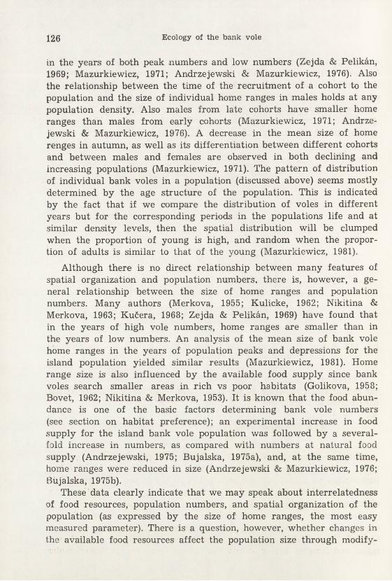
characteristic of the spatial organization of the population can, there­fore, be obtained by examining dynamic changes in the size of home ranges for individuals of different categories.

The home range was defined by Burt (1943) as the space surrounding a permanent dwelling of the animal, where it is searching for food, breeding, rearing the young. An individual inhabiting a relatively stable home range over its life span becomes familiar with it, and due to this it can find food easily and without large losses of energy, or a shelter from predators and adverse weather. The interest of ecologists in home ranges of small mammals, including bank voles, arose partly from the fact that there is a relationship between the size of home ranges as a species-specific characteristic determining spatial organi­zation of the population and other aspects of population organization (Brown, 1966; Bujalska, 1970, 1973, 1975a; Rajska-Jurgiel, 1976) its dynamics (Merkova, 1955; Naumov, 1956; Ryszkowski, 1962; Kulicke, 1962; Nikitina & Merkova, 1963; Koshkina, 1967; Kućera, 1068; Zejda & Pelikan, 1969; Mazurkiewicz, 1971), also competition (Andrzejewski & Olszewski, 1963a; Andrzejewski et a l , 1964; Aristova, 1970) and epizootic disease (Karaseva, 1956).

In studies on the size of home ranges, methods are a difficult issue. The same methods are used for bank voles as for other species of cryptic small mammals. Difficulties concern the reliability of the in­formation collected and with data processing method. Information on the size of home ranges, as the basic element of the spatial structure, can be collected by direct observation of animals or traces left by them, but most frequently the materials obtained from trapping by the CMR method are used for this purpose. In contrast to direct observations, which allow data collecting for only a small number of individuals, the CMR method provides information on almost all animals living in a given area. Another advantage of the CMR technique over direct observations lies in the fact that it also provides data on other popu­lation parameters (e. g. number dynamics, age and sex structure), thus it allows the observation of changes in spatial organization with refe­rence to these parameters.

6.3.1. Characteristics of Home Ranges

H o m e r a n g e s i z e . The size of a home range can be estimated from information on the places in which individual animals were trapped. As there are m any methods differring in their approach to the estimation of home range size, they will be reviewed below. In general, they can be classified into cartographic and statistical methods.

Structure of the population 119

The cartographic methods use the data collected to construct ts early as possible an exact distribution of the points at which individual ani­mals were caught to determine the size of their home ranges. For example, this group of methods is represented by the so-called “Minimum A rea” technique (Dalke & Sime, 1938; Mohr, 1947). It determines the surface area of the convex polygon containing all the points at which an animal was trapped.

Statistical methods determine the mean size of a home range by analysing the way in which the animal moves within it. Included here is the method of the greatest or the mean distance covered by an

Fig. 6.6. Home range of male 127, as calculated by different methods.* — trapping points, x >— points of effective capture, home range size in ha: polygon — 0.27, ellipse — 0.55, circle — 0.64, Wierzbowska’s method — 0.32, mean

distance as a radius — 0.04.

individual over the study period (Chitty, 1973; Godfrey, 1954; Brown, 1956) as a measure of the home range radius, or the method developed by Wierzbowska (1972), based on the relationship between the proba­bility of visiting particular trapping points by an individual and the size of its home range. Also the concept of a centre of individual acti­vity as the geometric centre of all the points of capture of an individual and changes in the probability of its capture with increasing distance from the centre (Hayne, 1949) prompted development of a theoretical model of the home range. Dice and Clark (1953) assumed in this model

X

120 Ecology of the bank vole

Table 6.4.The size of home ranges (in ha) in summer as estimated by

different authors.

Males FemalesYoung males

+ females Author Method of estimation

0.9 0.09--0.28 0.08—0.23 Aristova, 1970 not specified0.89—1.1 0.05--0.14 0.07—0.20 Nikitina &

Merkova, 1963 not specified0.10—0.45 0.02--0.25 0.01—0.33 Naumov, 1951 ))0.01—0.23 0.08--0.15 0.01—0.24 Golikova, 1958 J)0.20—0.88 0.16--0.56 0.12—0.84 Koshkina et al. 71

19722.00—2.20 0.19--0.32 0.10—0.25 Nikitina, 1961a0.77—1.39 0.13--0.20 0.13—1.18 Mazurkiewicz, elliptic model

19710.12—0.25 0.11--0.12 0.11—0.22 Mazurkiewicz, Wierzbowska’s

1981 method (1972)0.30—0.50 0.05 .— Radda, 1968 “Minimum Area”0.08—0 70 0.07--0.63 — Brown, 1956 Manville’s method0.02—0.48 0.02--0.63 .— Zejda & inclusive boundary

Pelikan, 1969 strip0.02—0.16 0.01--0.18 — Saint-Girons, not specified

1960a

that the general shape of a home range is circular, while Jennrich & Turner (1969) and Mazurkiewicz (1969) assumed an elliptical shape.

For example, the home range of a male bank vole has been calculated

Fig. 6.7. Seasonal changes in home ranges as calculated by different methods(1 = 225 m2).

1 — circle method, 2 — elliptic model, 2 — “Minimum area”, 4 — Wierzbowska’smethod, 5 — mean distance.

Structure of the population 121

using the methods listed above and by the mean distance covered over a two-week period. The results vary from 0.04 to 0.64 ha (Fig. 6 .6). Therefore, the choice of the method, which strongly depends on author’s views of space utilization by an animal, anticipates the results, this being frequently the case in ecology. There are many literature data on the size of home ranges for the bank vole, and they differ markedly because different methods were used (Table 6.4). Thus, absolute values of home range sizes should be considered as rough approximations. It seems, however, that the analysis of changes in the size of home ranges with time is not significantly affected by the methods used. This is shown in Figure 6.7 illustrating seasonal changes in the mean size of home ranges for males of an island bank vole population, as calculated by the methods discussed (Mazurkiewicz, unpublished data). Except for the mean distance method, which was insensitive, all the other methods show similar trends in changes of the size of home ranges, though at different mean levels.

25-

20 -

% 15-

10-

5-

a1.0 1.27 1.57 2.0 251 3.16 398 5.0 6.31 7.04 100

Relationship between ellipse axes

Fig. 6.8. Distribution of individual bank voles in relation to the degree of elonga­tion of their home ranges.

H o m e r a n g e s h a p e . Many data show that home ranges of the bank vole are frequently elongated, and the animals follow run along preferred paths (Tanaka, 1953; Mohr, 1965; Mazurkiewicz, 1971). Also maps of bank vole home ranges published in many papers to ana­lyze their size (Naumov, 1951; Karaseva, 1956; and others) concur. Such a param eter as shape makes it possible to examine the effect of environ­mental, biocoenotic, or intrapopulation factors inhibiting some directions of animal movements and enhancing others. Characteristics of the sha­

122 Ecology of the bank vole

pes of individual home ranges can be obtained using the elliptical model for estimating home range size. Such an analysis exist for more than 1000 bank voles of an island population (Fig. 6.8) (Mazurkiewicz, 1971), and for bank voles living in an open population (Mazurkiewicz, 1969) in order to eliminate the possible effect of the limited surface area of the island. In both cases, the shape of home ranges was elongated (the mean elongation expressed as the ratio of the ellipse axes was 2.5—3.6).

D u r a t i o n o f h o m e r a n g e s . In addition to the size and shape, the general characteristic of a home range should also include its existence in space and time. Duration influences the estimate of the home range size (if the home range is shifted during the study area, its size will be overestimated), as well as processes occurring in the po­pulation (see section on migrations). Usually, it is assumed that bank voles are characterized by a high site tenacity, and differences in the size of home ranges result from their seasonal shrinkage or extension (Naumov, 1951; Nikitina, 1970; Koshkina et al., 1972). Site tenacity may thus depend on age and sex of animals. Young bank voles are highly mobile until reaching m aturity, after which they establish and attache to home ranges (Smirin, 1965). This is particularly the case of adult females (Aristova, 1970). Adult males, however, shift home ranges while reducing or extending range sizes (Mazurkiewicz, 1971).

6.3.2. Spatial Organization in Relation to Population Structure and Dynamics

Home range in relation to a g e a n d s e x . Home range size is a function of the age and sex of animals, especially in overwintered animals. This variable area of utilization is probably related to their most important role in population reproduction. Differences in the home range size between males nad females are most acute in this group (Manville, 1949; Brown, 1965; Radda, 1968; Mazurkiewicz, 1971). The home ranges of overwintered males can be five to ten times larger than those of females (Naumov, 1951; Nikitina & Merkova, 1963). Also the degree of their elongation may be different. Males have very long ranges with an axis ratio of 3.0—3.6, while for females this ratio is 2.1—2.4 (Ma­zurkiewicz, 1971). Differences in both the size and the shape of home ranges between males and females prim arily result from their differential space utilization. Home ranges of females are better delimited and they do not overlap (Naumov, 1951; Ilyenko & Zubchaninova, 1963; Aristova, 1970; Bujalska, 1970). The distribution of home ranges of adult females is related to reproduction and the need for securing adequate food supply (Bujalska, 1973). Instead, the home ranges of males largely

Structure of the population 123

overlap. Differences in the size of home ranges between males and females can also be observed in even-aged groups of voles born in the current year, but they are not so drastic as in the case of overwintered animals (Naumov, 1951; Mazurkiewicz, 1971).

S e a s o n a l c h a n g e s . Changes in population numbers from spring through autumn are accompanied by changes in the spatial orga­nization of the population. In spring, when the population is made up only of overwintered animals, males occupy large and long home ranges located in several directions according to the location of female home ranges (Mazurkiewicz, 1971). A high mobility of males at that time (Smirin, 1965; Zejda & Pelikan, 1969) increases the frequency of contacts with females. Naumov (1951) found that males cover home ranges of several adult females, though two adult males have never been caught in the home range of the same female at the same time. Females have small, isolated home ranges and are less mobile (Radda, 1968), particu­larly during gestation and lactation (Nikitina & Merkova, 1963).

The position of generations entering the population from June to October within the spatial structure of this population depends on many factors. The most important seem to be the actual composition and density of the population at the time of the appearance of a new cohort, the abundance of this cohort and its role in reproduction (Naumov, 1951; Bock, 1972). In an island bank vole population a relationship has been found for males between the sequence of their recruitm ent to the population and the size of their home ranges (Mazurkiewicz, 1971; Andrzejewski & Mazurkiewicz, 1976). The later a cohort was recruited, the smaller were home ranges of males. Home ranges of females be­longing to different cohorts were similar. Also Bujalska (1970, 1973) found for the same population that the home ranges of m ature and immature females do not differ in size. However, according to Naumov (1951), home ranges of adult and subadult females are 1.5 to 2 times larger than those of young females. In new cohorts as in overwintered animals, the home ranges of males are larger than those of females (Fig. 6.9). The shape of individual home ranges in particular cohorts shows irregular changes with time and it tends to “round out” from spring to autumn (Mazurkiewicz, 1971).

After the breeding season, such features as age and m aturity of population members and their participation in reproduction have less effect on the spatial structure of the population. Consequently, in autum n a decline is observed in the differentiation of the size of home ranges between cohorts and of the two sexes. The smallest home ranges occur in winter (Saint-Girons, 1960a; 1961; Ilyenko & Zubchaninova,9 — Acta therio logica

124 Ecology of the bank vole

1963; Nikitina & Merkova, 1963) when bank voles are most sedentary. At the end of winter, prior to the breeding season, individual home ranges are increasing (Ilyenko & Zubchaninova, 1963).

S p a t i a l d i s t r i b u t i o n o f i n d i v i d u a l v o l e s . In the literature there are data indicating tha t individual bank voles tend to occur in aggregations because of habitat heterogeneity (Bock, 1972) or interspecific competition (Naumov, 1948; Larina, 1957; TurCek, 1960; Krylov, 1975). Differences in the size of home ranges related to the age

12-

i---------------- 1-----------------1---------------- 1---------- — r *Morch June July Sept. Oct.

Fig. 6.9. Seasonal changes in the size of home ranges of different generations(1 = 225 m2).

and time of recruitment of individual bank voles to the population (Nau­mov, 1948; Mazurkiewicz, 1971) show that there are some spatial relation­ships among individuals of different age-classes. This is also indicated by differences in the distribution of individual voles in an island popu­lation with reference to the population density and the proportion of young animals (Mazurkiewicz, 1981). A clumped distribution is observed in this population in spring at low density (about 20 voles/ha). This is an effect of a high activity of males on the island, which occupy large widely overlapping home ranges at that time. Mature females, however, are rather evenly distributed (Bujalska, 1970). A tendency towards

Structure of the population 125

clumping at low population densities of the bank vole was also observed by Krylov (1975). In summer and autum n the general character of the distribution of individuals in the population depends on the proportion of young voles in it. Bujalska (1970), who analysed the distribution of mature and immature females, found that the latter had a clumped distribution. Also the general analysis of the distribution of bank voles on the island shows that the clumped distribution occurs when the youngest individuals are several times more abundant than adults (Fig. 6.10).

individuals

P lg. 6.10. A relationship between the degree of clumping and the proportion oI young individuals in the population (r = 0.871, p > 0.001).

Therefore, in addition to the environmental factors mentioned above, the age and sex structure of the population im portantly determines the distribution of bank voles.

6.3.3. Vole Numbers in Relation to Spatial Organization of the Population

Patterns of number dynamics in bank vole populations vary from year to year, and as a result, population numbers can be high or low (see section on population dynamics). Let us try to see whether and to what degree the spatial structure of the population varies in the years of differing population numbers.

It seems that some features of the spatial structure do not depend on the total population size, thus they are constant to some degree. One of these features is the differentiation of home ranges between males and females. Males always take larger home ranges than females

126 Ecology of the bank vole

in the years of both peak numbers and low numbers (Zejda & Pelikan, 1969; Mazurkiewicz, 1971; Andrzejewski & Mazurkiewicz, 1976). Also the relationship between the time of the recruitm ent of a cohort to the population and the size of individual home ranges in males holds at any population density. Also males from late cohorts have smaller home ranges than males from early cohorts (Mazurkiewicz, 1971; Andrze­jewski & Mazurkiewicz, 1976). A decrease in the mean size of home renges in autumn, as well as its differentiation between different cohorts and between males and females are observed in both declining and increasing populations (Mazurkiewicz, 1971). The pattern of distribution of individual bank voles in a population (discussed above) seems mostly determined by the age structure of the population. This is indicated by the fact that if we compare the distribution of voles in different years but for the corresponding periods in the populations life and at similar density levels, then the spatial distribution will be clumped when the proportion of young is high, and random when the propor­tion of adults is similar to that of the young (Mazurkiewicz, 1981).

Although there is no direct relationship between many features of spatial organization and population numbers, there is, however, a ge­neral relationship between the size of home ranges and population numbers. Many authors (Merkova, 1955; Kulicke, 1962; Nikitina & Merkova, 1963; Kućera, 1968; Zejda & Pelikan, 1969) have found that in the years of high vole numbers, home ranges are smaller than in the years of low numbers. An analysis of the mean size of bank vole home ranges in the years of population peaks and depressions for the island population yielded similar results (Mazurkiewicz, 1981). Home range size is also influenced by the available food supply since bank voles search smaller areas in rich vs poor habitats (Golikova, 1958; Bovet, 1962; Nikitina & Merkova, 1953). It is known that the food abun­dance is one of the basic factors determining bank vole numbers (see section on habitat preference); an experimental increase in food supply for the island bank vole population was followed by a several­fold increase in numbers, as compared with numbers at natural food supply (Andrzejewski, 1975; Bujalska, 1975a), and, at the same time, home ranges were reduced in size (Andrzejewski & Mazurkiewicz, 1976; Bujalska, 1975b).

These data clearly indicate that we may speak about interrelatedness of food resources, population numbers, and spatial organization of the population (as expressed by the size of home ranges, the most easy measured parameter). There is a question, however, whether changes in the available food resources affect the population size through modify­

Structure of the population 127

ing its spatial structure, or whether the character of the spatial structure is an effect of the population numbers, which is directly determined by the available food supply. In the first case the increase in food resources accounts for a decrease in the area covered by animals in search of food (an adequate food supply can be found within a smaller area). As a result, agonistic interactions among m ature females may be reduced and, consequently, more females may have chances to repro­duce than in the case when food resources are scarce (Bujalska, 1975b). A high birth rate and high infant survival result in a significant in-

Fig. 6.11. Possible effects of ecological factors on the size of home ranges.

crease in numbers (Bujalska, 1975a). In the second case, abundant food supply has a direct effect on population numbers through a positive effect on the condition of animals (Andrzejewski, 1975) and their low mortality (Bujalska, 1975a, 1975b). The increase in population density intensifies agonistic intraspecific interactions and, as a result, leads to a reduction of the area they search. Both possibilities seem to be equally probable in the light of the data presented above. It is also possible that both are realized at the same time. The considerations presented above on the role of the spatial structure in the life of the population and individual animals are schematically illustrated in Figure 6.1.1.