J . Fluid MIA. (1981), wZ. 109, pp. 1-24

P r i M in Great Britain

1

Structure in turbulent mixing layers and wakes wing a chemical reaction

By R. BREIDENTHAL Guggenheim Aeronautical Laboratory, California Institute of Technology, Pasadena

(Received 7 March 1980)

Plane turbulent mixing between two streams of water which contained dilute chemical reactants was studied in anew blow-down water tunnel. In a diffusion-limited reaction, a pH indicator, phenolphthalein, in one stream mixed and reacted with a baae, sodium hydroxide, in the other stream to form a visible reaction product. The product was found to exist, as expected, in concentrated regions associated with the large, @an- wise-coherent structures of the turbulence. A transition in the mixing was observed in which the aqueous mixing product increased by an order of magnitude. The transi- tion is a consequence of the appearance and development of small-scale three- dimensional motions in the flow. Downstream of the transition, the amount of mixing product was independent of Reynolds number (for an order-of-magnitude increase in the latter) and at most only weakly dependent on Schmidt number.

1. Introduction Turbulent mixing layers are one of the simplest turbulent shear flows and, as such,

have proved to be useful in attempts to understand the nature of turbulence. Indeed a major revision in thinking has followed the discovery and recognition of coherent large-scale structures in turbulent mixing layers (Brown & Roshko 1974; Winant & Browand 1974; Roshko 1976; Dimotakis & Brown 1976). Subgrid scale modelling and other predictive schemes, which incorporate observed aspects of the large structures, are being developed. Because of the mixing layer’s relative simplicity and technological significance, it is still a fruitful subject for research.

A shear layer (figure 1 a) is formed when two parallel flowing streams with different speeds begin to mix downstream of the trailing edge of a splitter plate partition. When the two streams have the same speed, a wake (figures 1 b, c) is formed instead. During the course of these experiments, both shear layers and wakes were studied using a splitter plate with a sharp trailing edge, as well as wakes from a thick, blunt splitter plate. An important property of a turbulent mixing layer is its ability to mix fluid from

each stream at an intimate, molecular level. While the velocity field of the flow has been studied for some time, it is only recently that the mixing has been measured. Using a small gas-sampling probe, Konrad (1977) inferred the amount of molecular scale mixing in a mixing layer between two gas streams. His results were based on the idea that, if each s t r a m carried a dilute chemical reactant and the reaction kinetics were very fast and irreversible, then the amount of chemical product would correspond to the amount of molecular scale mixing at the reaction equivalence ratio. Such a

2 R. BreidenthQl

(4)

UI - - uz= u,= u

FIUURE 1. (a) Plane mixing layer. (a) Plane wake, thin trailing edge. (c) Plane wake, thick trailing edge.

chemical system is an important limiting case of other systems, e.g. combustion with heat release or slower chemical reactions.

The ultimate step in the mixing process between two streams is molecular diffusion of one reactant toward another. A primary question that motivated the present work is ‘what is the effect of the molecular diffusion rate on the mixing rate? ’, that is, the rate of production of product. Schmidt number (Sc = v / 9 ) is the ratio of two diffusion coefficients, that of vorticity or momentum to that of matter. It is in the nature of gases that their Schmidt numbers are almost always near unity, whereas liquids like water have Schmidt numbers three orders of magnitude larger. Thus one objective of the experiments was to explore the influence of Schmidt number (and therefore molecular diffusion) on the mixing in an aqueous shear layer (Sc = 600) by comparing the results from Konrad’s experiments in gases (Sc = 0.7).

The inert sampling technique of Konrad is difficult in water because of the small sampling volume required to resolve the high concentration gradients which result from the slow aqueous diffusion rate. Instead, the molecular scale mixing could be measured directly by letting a chemical reaction between the two streams produce an easily detectable reaction product. The optimum reaction would produce a

Chemical reaction in turbulent mixing layers and wakes 3

visible reaction product which could be detected optically without intrusion into the flow.

Furthermore, the visible reaction product offers a unique flow visualization because it directly displays the mixed fluid. In contrast to an inert dye or smoke which simply diffuses away in the interesting regions of intense mixing, the visible reaction product is produced there. It is a complementary technique to conventional flow visualization and offers a potentially new view of flows which have heretofore been visualized with only conventional schemes.

Broadwell (see Witte et al. 1974) proposed a simple mixing model which predicts the effect of Schmidt number as well as Reynolds number on the mixing. The mixing process is visualized as a sequence of events which begin with the entrainment of a large blob of fresh reactant into the layer (Brown & Roshko 1974). The blob is broken down into smaller and smaller sized lumps until the Kolmogorov microscale A,, is reached. Two time scales can be defined: a large-scale entrainment (and breakdown) time 6lAU and a microscale diffusion time h g / 9 , where AU = U,- U, is the velocity difference between the two free streams and 6 is the vorticity thickness of the layer, AU/(au/ay),,,. The ratio T of these two times is T N (Ag/B)/(c?/AU) N (SclRet), where Re _= AU6/v - Re-% from Kolmogorov’s argument. When T 9 1, small-scale diffusion causes the ‘bottleneck’ in the mixing, while, for T 4 1, entrainment is the rate-limiting step. A slightly more refined argument which integrates the total time from entrainment through breakdown to the microscale yields essentially the same result. If the mixing is entrainment-limited, then the amount of product should be independent of Reynolds number and Schmidt number.

2. Apparatus The design philosophy was to construct a simple, general-purpose apparatus which

could be operated by one person and easily modified to vary the test-section flow conditions. A large-scale Reynolds number of at least Re = A U&/v = lo4 was desirable for a comparison with the high Re gaseous results. For a fixed velocity ratio, Re varies like the characteristic test-section dimension while the volume flow rate goes like its square. In the interest of conserving reactant chemicals and reservoir volume, a relatively small test section was chosen, 7 x 11 cm span and 45 cm long. With a design speed of 300 cm s-l, the goal of Re = lo4 was achieved with a relatively small expendi- ture of reactant solution.

Since the reactants would mix and react in the test section, a closed-circuit tunnel was not feasible. Rather, a simple gravity-driven, blow-down configuration was chosen, with the reactant solutions prepared in batches before a run.

A schematic sketch of the apparatus is shown in figure 2. Each reservoir has a capacity of about lo3 1, permitting a 30 s run at the design speed of 300 cm s-l. Owing to the relatively small change in water level, the flow speed changes by less than 2 % in 10s. Steady-stat,e flow is typically established in 2-4s. The free-stream turbulence intensity (u’2/U2)f was measured by a laser-Doppler velocimetert to be slightly less than 0.5% at the beginning of the test section for several tunnel speeds spanning the velocity range studied.

t With the help of Mr Manooch Mohseni-Koochesfahani and Dr Keith Koenig.

4 R. Breidenthal Reservoir tanks

Honeycomb, screens, etc. r

Control valves I/

FIQURE 2. Sketch of the apparatus.

The nozzle contour is defined by tangent circular arcs, 48 and 11 cm radius, with the latter tangent t o the test section. The ‘thin’ splitter plate is a wedge of 8” total angle whose trailing-edge thickness is less than 0-003 cni. A ‘thick ’ splitter plate is a trunc- ated wedge of the same length whose trailing-edge thickness is 0.635 cm.

A stainless-steel traversing mechanism, driven by a digitally controlled stepping motor, can move a Pitot tube probe in increments of 0.0066 cm across the test section to measure mean velocity profiles.

3. Measuring techniques 3.1. Passive scalar technique

The amount of molecular-scale mixing in a turbulent shear layer between two streams could be measured in a t least two ways. Perhaps the most obvious approach is the passive scalar contaminant technique illustrated in figure 3. An inert scalar, for example a blue dye, is introduced into one reservoir. A diffusion interface always exists within the mixing layer which separates the blue fluid from the clear, undyed stream. Within the interface the blue dye diffuses into the clear fluid; all the molecular- scale mixing occurs within the interface.

Using this technique the amount of blue dye within a small sampling volume would be measured as a function of time. If the sampling volume were small enough to measure the true, local concentration of the inert dye, it would be possible, using Toor’s analysis (Toor 1962) to infer the amount of chemical product that would be formed if each stream contained dilute reactants which rapidly react in an irreversible reaction. On the other hand, if the sampling volume is not small compared to the smallest concen- tration scales, i.e. the interface thickness, then the probe will smooth out the actual concentration fluctuations and thus overest,imate the amount of product formed. The inert technique always yields an upper bound on the actual molecular-scale mixing

Chemical reaction in turbulent mixing layers and wakes b

FIGURE 3. Inert scalar technique.

(in contrast to the reaction technique, described below, which gives a lower bound). The diffusion interface can become quite thin in a high-Schmidt-number fluid like

water. For typical high-Reynolds-number conditions in the present apparatus, the interface is estimated to be as thin as the wavelength of light (thickness - (9/uo)*, where uo N (AU/&)Re* is the Kolmogorov scale strain rate). If so, it is difficult to construct even an optical sampling volume with dimensions small compared to the interface thickness. The interface could be several orders of magnitude thicker and still present a difficult problem experimentally. Of course, one could achieve a high- Reynolds-number flow by building a very large apparatus with flow speed so low that the diffusion interface would be thick compared to an obtainable probe size. This approach, however, was not practical.

3.2. Chemical reaction technique

The problem of finite probe size would be solved if a process could be found which would measure the mixing at the molecular level and macroscopically display the correct answer independent of the interface thickness. Such a process is a second-order chemical reaction: A + B+ C. If dilute reactant A is added to stream one, and B to stream two, and if they rapidly react in an irreversible manner when mixed at the molecular level to form a reaction product C (an ‘ideal’ reaction), then the amount of product formed is just equal to the amount of molecular-scale mixing between the two streams at the reaction equivalence ratio. Further, if the reaction product happens to be visible, then the amount of mixing can be measured optically, in a non-obtrusive way.

In contrast to the pasgive case, the finite size of the sampling volume in the reacting flow does not inherently overest,imate the amount of mixing (see figure 4). If the reaction is ‘ideal ’, then the total amount of mixed fluid at the reaction equivalence ratio within the sampling volume is just equal to the total amount of product there, no matter how big the sampling volume, or how thin the diffusion interface. Integrating is experimentally easier than differentiating. This attractive characteristic permits accurate aqueous mixing measurement.s a t fairly high Reynolds numbers in a reason- ably sized laboratory apparatus.

An ideal, irreversible reaction was not found; instead, it was approximated by a reversible one. (Thus the mixing inferred was a lower bound.) Phenolphthalein, a

6 R. Breidenthal

FIGURE 4. Reacting technique.

common pH indicator, reacts with a base, sodium hydroxide, in a complex series of steps (Kolthoff 1937). The overall reaction is

phenolphthalein + 2(OH)-+ red product. ( 3 4

The reaction, while not ideal, was chosen for several reasons. It is believed to be diffusion-limited in the chemical sense and is thus very fast (Czerlinski & Eigen 1959; Caldin 1964). The reactants are more or less water soluble, non-toxic, inexpensive and transparent. The red product is strongly visible so that dilute concentrations are sufficient for detection. Dilute reactants are unobtrusive so that the turbulence is unaffected by the chemistry, i.e. there is little surface tension, buoyancy, heat release, etc.

The experiments were performed at an equivalence ratio of about lo2, with an excess of (OH)-. This was dictated by the pH transition range of phenolphthalein and its limited solubility in water. The free-stream phenolphthalein concentration was about 1 0 - 5 ~ and the pH of the alkaline solution was about 11.7. This value was chosen to minimize reversibility effects and the disappearance of red product due to another reaction at very high pH levels (see appendix).

The amount of red product was measured by the attenuation of a narrow beam of green light (see figure 5 ) which passed through the layer, oriented normal to the plane of the layer. The beam width was defined by two apertures, ranging in diameter from 160 to 2000pm. A narrow-band optical filter (35 A half-maximum bandwidth) selected the 5461 A green mercury line of the light source, which is near the phenol- phthalein red product absorption maximum of 5530 A.

An effective product thickness P was defined in a manner similar to a boundary- layer displacement thickness

The integral of the product concentration along the light beam, normalized by the free-stream concentration of reactant B (phenolphthalein) is the equivalent thickness of the amount of product in the layer, and can be compared to the vorticity thickness& The ratio PIS is, roughly speaking, the fraction of the layer filled with mixed fluid.

Chemical reaction in turbulent mixing layers and wakes

Mercury-argon lamp

7

I Lucite window 7

-*- 4 Beam expander lens

1 Photomultiplier tube (for calibration only)

FIGURE 5. Optical system.

4. Flow visualization As mentioned in the introduction a very useful advantage of the visible reaction

product is the unique flow visualization it affords. The slow diffusion rates of vorticity and matter in water are well-known advantages in conventional flow visualization, permitting lower flow speeds for a given Reynolds number and higher-resolution photographs.

Perhaps the most intriguing feature of reacting flow visualization is the relationship between vorticity and chemical product. Initially, the vorticity and product are both concentrated in thin sheets at the splitter plate trailing edge. Both convect with the flow and diffuse down their concentration gradients (at different rates if Sc 1). In a two-dimensional, constant-density flow vorticity is not st,retchedand behaves just like a scalar contaminant, satisfying the Eulerian heat equation

DO -- - vv2w. Dt

The local vorticity thickness, Glocal, for an isolated sheet in two-dimensional flow is just proportional to the local product thickness P times Sc), since both behave like scalar contaminants diffusing at different rates. The actual instantaneous distri- butions of vorticity and product within the sheet are not identical (figure 6), since product is continually being produced a t the reaction surface, whereas vorticity is not. (An inert dye would, however, label the vorticity provided Sc = 1.) Thus, within the sheet, vorticity is not precisely labelled by product, even for Schmidt number unity and two-dimensional flow.

As long as the sheet is isolated, i.e. its thickness is small compared to both its radius

8 R. Breidenthal

FIQURE 6. Product and vorticity distributions within the interface.

of curvature and the distance to any other near-by sheets, the maximum vorticity surface near the centre of the sheet will approximately coincide with the reaction surface, the surfaoe of maximum product. In this global sense, the product labels the vorticity for an isolated sheet, regardless of Schmidt number.

If the sheet is not isolated, ‘flame shortening’ (Marble & Broadwell 1977) and the analogous ‘vortex sheet shortening’ effects can alter the ratio (P/S)local. And, if the flow is three-dimensional, vortex stretching will amplify and rotate the vorticity vector. The ohemical product is not amplified by stretching, of course, since it is a scalar.

In spite of the fact that the product does not precisely label the vorticity because of flame-shortening and vorticity-stretching effecbs, it may nonetheless approximately label it globally. Stretching only can amplify vorticity where vorticity already exists. One might argue that for Sc > 1 vorticity can diffuse into an irrotational region faster than the product and then be amplified there by stretching to a very large absolute value. While such events must be common, if the Reynolds number is reasonably large the vorticity cannot diffuse very far compared with the large scales in the turbulence. The viscous length is small and convection rather than diffusion dominates the transport of vorticity. From a global view, then, the chemical product may approximately label t,he vorticity.

4.1.

(a) #hear-layer flow pictures. A side view of the reacting shear layer is shown in figure 7(a). The lower stream is coloured with an inert blue dye which appears as light grey in the monochrome photograph. The upper, high-speed stream is trans- parent so that the entrainment of the blue and clear fluids into the layer is visible. The reaction product is red (dark grey in monochrome) and resides in regions associated with the large vortical structures. The photograph strongly implies that these vortices dominate both the mixing and the distribut,ion of mixed fluid, at least for these flow conditions.

Figure 8 is a plan view of the flow in the transition region. Several features of the photograph are significant. The basic two-dimensionality of the instantaneous product distribution is evident. The flow near the side walls is somewhat disturbed. When this was first observed, it was thought to be an inherent feature of the shear-layer inter- action with the wall. However, it may also be due to a secondary flow which is produced in the corners of the test section by the upstream nozzle contraction, resulting in a perturbed wall region. In any event, the flow near the test section centre-line appears reasonably clean, and all measurements were made there.

Chemical reaction in turbulent mixing lagers and wakes 9

(C)

FIGURE 7. Reacting shear layer and thick wake. (a) U, = 37 cm s-l (top strcam), T = 0.36. ( b ) U d / v = 200. (c) U d / v = 1.6~ lo4.

( b ) The wiggle disturbance. The most interesting feature of figure 8 is the spanwise- sinuous disturbance. Upstream of the ‘wiggle ’ the flow is two-dimensional. Streamwise lines are visible downstream of the wiggle and the flow is clearly three-dimensional there, although t’he large-scale structures maintain their spanwise coherence.

Similar streamwise streaks have been observed by shadowgraph photography in

10 R. Breidenthal

# I m

FIG

UR

E 8. P

lan

vie

w o

f th

e w

iggl

e, U, = 3

8 cm

a-',

r

= 0.38.

Chemical reaction in turbulent mixing layers and wa.kes 1 1

the Brown-Roshko gas apparatus for some time (Konrad 1977). They have been interpreted as streamwise vortices of alternating sign. Their origin was, however, obscure. In figure 8 another wiggle is apparently evolving in the neighbouring vortex upstream of the wiggle. The outer sheet of the vortex is corrugated, while the inner sheet appears relatively unperturbed. It is tempting to conclude that this is charac- teristic of the wiggle formation. The average wavelength of the sinuous wiggle was measured from photographs to be about 1.1 times the wavelength of the initial two- dimensional Kelvin-Helmholtz waves. After the wiggle is formed, it is stretched by the global strain field of the flow. Its amplitude grows rapidly, while its wavelength remains constant. There are indications of this process in figure 8. As discussed by Bernal et al. (1979) and Breidenthal(1979), the wiggle is not always nor at all conditions the only way in which three-dimensionality is introduced into the flow.

A time exposure of the plan view is shown in figure 9. The streamwise streaks represent long-time-averaged spanwise variations in the mixing. The streaks first appear at the onset of the wiggle and extend to the end of the test section. The relative amplitude of the spanwise variations appears to be maximum a short distance down- stream of the wiggle location.

A photograph of the plan view at large Reynolds number (figure 10) demonstrates that, despite the presence of strong three-dimensional, small-scale motions in the flow, the large structure is basically two-dimensional, as indicated by the product distri- bution.

4.2. WakeJlow pictures The thick wake is shown in figure 7 (b, c) (plate 1). At low values of Re, = U,d/v the thick wake is laminar and forms a plane interface downstream of the base flow closure region. As the Reynolds number increases, the familiar wake behaviour of quasi-two- dimensional vortex shedding is apparent. Three-dimensional motions appear a t Re, = 150 to 200. Further increase in Re, results in a highly three-dimensional, small- scale field superimposed on the quasi-two-dimensional large-scale vortex street.

5. Product measurements 5.1. Shear-layer time histories

As discussed in $3.2, the amount of product was measured by passing a narrow beam of light through the layer normal to its plane. The red product attenuates the beam, allowing the instantaneous amount of product along the light path to be calculated and recorded as a function of time. Time histories of the equivalence product thickness P (equation 3.2) are shown for two Reynolds numbers in figure 11. The shear layer has about the same thickness in both runs, yet the average value of P (indicated on the vertical axis) is much higher a t the larger Reynolds number. The cause of this mixing transition is the presence of small-scale three-dimensional motions a t large Re. There are impressively large fluctuations in the instantaneous value of P a t the higher Reynolds number, the large excursions corresponding to large vortex structures convecting through the beam. The average time interval for the passage of t,he large st,ructures is indicated, where 1 is the mean vortex spacing.

Figure 12 is a similar time history of P above the transition but with a compressed time scale. Electronic noise accounts for occasional excursions of the signal below

12 R. Breidenthal

d

FIQ

UR

E

9. T

ime

exp

osu

re o

f th

e pl

an v

iew

U, =

38 cm 8

-1,

r =

0.37.

Chemical reaction in turbulent mixing layers and wakes

l-

0 c?

13

FIQ

UR

E

9. T

ime

exp

osu

re o

f th

e pl

an v

iew

U, =

38 cm 8

-1,

r =

0.37.

14

10 -

8 -

E 3 6 -

Y 0 4 - .c

-.

Y

-0

2 -

R . Breidenthl

101 w

(a ) (b )

FIGURE 11. Time histories of the product thickness for the shear layer. (a) U , = 35 cm s-l, r = 0.36, x = 14 cm. ( b ) U, = 257 cm 8-1, r = 0.35, x = 15 em.

l 0 1 9 1 101 U I

Time - 1 s record

FIGURE 12. Time history with a compressed time scale. U, = 465 cm s-l, r = 0.37, z = 14 cm.

the axis P = 0. Many large structures have passed through the beam during this long record. At several sampling times during the record the light beam detected almost no product, indicating that it is occasionally possible to see almost entirely through the layer even a t large Re, cf. figure 10. Topologically, of course, there must always be a reaction interface and thus a finite amount of product between the two reactant fluids. However, because of high local strain rates in the turbulence this interface may locally be very thin in a high-Schmidt-number fluid and thus contain very little product. If the light beam pierces only one such thin interface at some instant, then the instantaneous product thickness is very small.

Chemical reaction in turbulent mixing layers and wakes 15

0.6 la . 4, 1

0.4

0.2

n ., 102 103 104

AU6/v

FIQURE 13. Effects of lerge-scale Reynolds number, Schimdt number and velocity ratio on the mixing. a, r = U,/lJ, 0.76, Sc t 600; 0, r = 0.38, Sc t 600.

5.2. Effect of Schmidt number The main results of the mixing measurements for a velocity ratio of r = 0.38 are shown in figure 13 and have been briefly reported previously (Breidenthal 1979). The (mean) equivalent product thickness P normalized by the vorticity thickness 8 is plotted as a function of large-scale Reynolds number Re = AU8/v. The full-line curve is inferred from Konrad's (1977) results for a shear layer between two different gases. The highest equivalence ratio f that Konrad discussed was 10, while the phenol- phthalein chemistry constrains the present work to an equivalence ratio of a few hundred. Fortunately, Konrad found that the mixing in his experiment appears to approach its asymptoticvalue at an equivalence ratioof 10, and little changeisexpected for larger values off. The physical explanation is that for a large enough equivalence ratio the amount of product formed is just limited by the entrainment of the scarce reactant into the layer, since there is an abundance of excess reactant there. Thus in figure 14 the present work at f w 200 can be compared with Konrad's results for f = 10.

The most obvious feature is the rapid increase in PI8 at Re = 5000. At the transition PIS jumps about 250/, in the gaseous flow and about a factor of 7 in the aqueous layer.

Above the transition the amount of mixing is seen to be independent of Reynolds number and only a weak function of Schmidt number. The Schmidt number differs in the two cases by three orders of magnitude, yet PI8 changes by about a factor of 2 or less. Konrad employed the inert scalar contaminant technique which, as discussed in $3.1, always yields an upper bound on the actual mixing. In the present study, the chemistry is reversible and the light beam is of finite width, so that the aqueous measurements are a lower bound on the mixing. Since the gaseous and aqueous measurements are upper and lower bounds, respectively, on the mixing, it is possible that the actual difference in mixing at high Reynolds number is considerably less than indicated.

Below the transition, the mixing is a strong function of Sohmidt number. The gas and water measurements differ by about a factor of 12 here. If there are no Aame-

16

0.5

0-4

0.3

--. 4

0.2

0.1

R. Breidenthal

1 1 I I 1 1 1 1

O 20 I a V

FIGURE 14. Effect of initial Reynoldsnumber on theshear-layer transition. Values of r ( = U,/U,) : 0, 0.38; 8, 0.45; V, 0.50; 0, 0.57; m, 0.62; L] 0.67;u, 0.76;0, 0.80.

shortening effects, the mixing should vary like Sc-2 even though the vortex sheet is convoluted. The observed mixing difference in the two fluids is somewhat less than this; therefore there may be flame shortening in the gaseous flow. The effect should not be too surprising. Since Sc - 1 for the gas the local product and vorticity sheets are about the same thickness, ignoring the initial boundary layers. (As the flow isinitislly two-dimensional, no appreciable vortex amplification by stretching can occur.) If the vortex-sheet radius of curvature a t the vortex core is about equal to the sheet's local vorticity thickness there, then the sheets are not isolated and flame shortening can occur. I n addition to flame Shortening another possibility is experimental error associated with the aqueous measurements. P i s estimated to be of the order of 500,um at low Reynolds number. Since the mixing is so slight, modest absolute inaccuracies yield large relative errors.

It is interesting to compare the results for a, shear layer with the work of Weddell (1941), who explored the mixing in a reacting, aqueous jet. A red solution of phenol- phthalein and sodium hydroxide was injected into tank of sulphuric acid solution from an axisymmetric nozzle. When the injected fluid mixed and reacted with the ambient solution, the red phenolphthalein became transparent and disappeared (the reverse reaction to the one employed in the present work). Weddell measured the visual length of the red jet from its origin to the station a t which it disappeared and found that this reaction length became independent of jet Reynolds number above a Reynolds number of a few thousand. This result implies that the jet mixing is entrain- ment limited. Similarly in the present shear-layer results the mixing becomes entrain- ment limited when the three-dimensional, small-scale motions are established.

If the time-scale argument of Broadwell is correct (see 8 1 ) then some difference in the gaseous and aqueous mixing results for Re - lo5 is expected. I n the gaseous experiments, T = Sc/Rei - while in the present aqueous work T - 1. Thus in the aqueous flow the entrainment time is comparable to the small-scale diffusion time so that the mixing rate may be rcduced by delays from both processes. Un-

Chemical reaction in turbulent mixing layers and wakes 17

fortunately, in order to match the gaseous value of T - lo-, in water, an aqueous Reynolds number of order 4 x 109 is required. Broadwell's argument predicts that a t this Reynolds number the gas and water mixing rates should be identical. For 105 < Re c 109 the aqueous mixing would be a very weak function of Re.

A somewhat different argument supposes that convection a t the Kolmogorov microscale A, contorts the reaction interface since the latter is the smaller of the two for Sc > 1 . The interface thickness hi is the Batchelor microscale (Batchelor 1959) and is of order Sc-$A, (see $3.1). The ratio of Batchelor diffusion time to breakdown time is (A?/g)/(a/AU) - Sc-lT G Re-4 independent of Schmidt number. This question will be explored in a future paper.

5.3. Effect of initial conditions

Figure 13 also demonstrates the effect of freestream velocity ratio on the mixing transition. As r = U,/Ul is increased from 0.38 to 0.76, the transition Reynolds number AUd/v decreases. Thus the transition does not occur a t a constant large-scale Reynolds number, implying that the three-dimensional transition is influenced by the initial conditions of the laminar vortex sheet.

Since the mixing transition is evidently influenced by the initial conditions of the shear layer, the normalized product thickness PIS was plotted as a function of the initial Reynolds number U18,/v at a fixed x for 0.38 < r < 0.80 (figure 14). The curve in the figure represents thin-wake data ( r = 1) and is discussed in $5.5. This particular Reynolds number was chosen as the abscissa because (i) most of the vorticity in the initial vortex sheet originates in the boundary layer of the high-speed side when r = U, f U, < 1, and (ii) most of the opposite-sign vorticity from the low-speed boundary layer is quickly cancelled by diffusion of the high-speed vorticity. When r approaches unity, the two boundary layers are nearly symmetric so the choice of either one (or both) to characterize the initial conditions is clearly arbitrary. The initial vorticity thickness 8, was estimated as

where xCf f is the effective origin of the laminar boundary layer in a zero pressure gradient, The value of xe.f was estimated to be 4 cm for this apparatus. There is con- siderable scatter in the data, especially at low Reynolds number and especially in the transition region, reflecting the sensitivity of the mixing to small-scale motions and the streamwise streaks in the transition. Even so, i t is apparent that the transition occurs at about the same initial Reynolds number C\O,/v for velocity ratios from r = 0.38 to r = 0.80. The result lends support to the conclusion that the mixing transition is determined by the initial conditions. The momentum thickness 0, may not, of course, be the exact measure of the vortex-sheet thickness to define the transi- tion Reynolds number, but it is a reasonable first approximation. Note that another parameter based on initial conditions x / O , varied with the flow speed. This point will be discussed in G .

6.4. The three-dimensioml instability

There are at least three candidates for the initial instability which results in the tviggle. The M'idnall instability (Widnall, Bliss 8: Tsai 1974; Moore 8: Saffnian 1976; Tsai & \T'itlnall 1 Wci: Snffnian 1978) lvas first ~wo~)osed to explain cirriinifcrc~uti;il WLI-CS i n

18 R. Breidenthal

( C ) ( d )

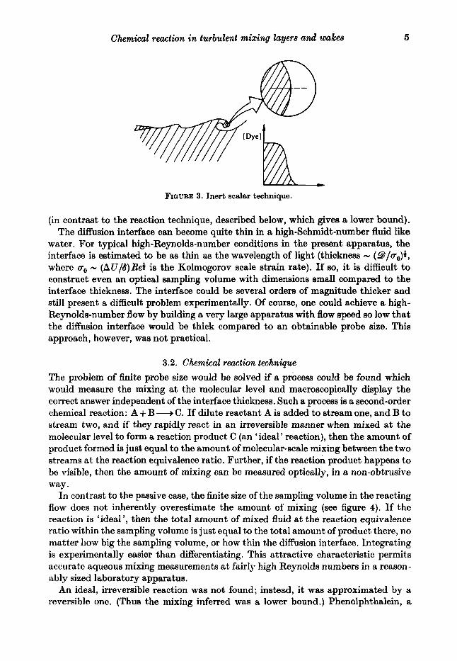
FIGURE 15. Thick-wake time histories, T = 8.5 cm. (a ) U d l v = 220; ( b ) U d l v = 2200; ( c ) U d l v = 4200; ( d ) U d l v = 15200.

vortex rings and, as suggested by Saffman (private communication), may be responsible for the wiggle in the shear layer. Briefly, the physical idea is that, if a rectilinear line vortex is perturbed into a sinusoidal shape such that the vortex is steady under its own self-induced velocity, then in the presence of an external strain field the crests of the deformed line vortex are convected away from their unperturbed position as a consequence of the imposed strain. In this way the amplitude of the sinuous pertur- bation grows with time.

Benney (1961) and Corcos (1979) employed fornial mathematical perturbation expansions t o explore the infinitesimal three-dimensional instability. Brown (private communication) and Konrad ( 1977) have suggested that the Rayleigh-Taylor instability is responsible for the streamwise streaks. Their shadowgraph flow visualiza- tion did not display the wiggle, so their model does not directly incorporate it.

Further work is needed to determine which, if any, of these candidatcs is the initial three-dimensional instability in the shear layer. Of course, different, instabilities may conceivably occur depending on the initial conditions and Reynolds number.

5.5. Wake mi.eing

The mixing in two different wake flows was briefly explored to compare with theshear- layer behaviour (see figure 1).

Figure 15 shows some typical time histories of the product thickness of the thick wake a t x = 8.5 cm for four different wake Reynolds numbers U d l v . The signal was quite periodic for U d l v = 220 and became less so as the Reynolds number increased. The average amount of product thickness, indicated on the vertical axis in each case, increased monotonically with Crdlv in the transition range, as shown in figure 16. The normalized product thickness PI& is plotted as n function of the large-scale wake

Chemical reaction in turbulent mixing layers and wakes 19

I I I I 1

0.3

Pl6,

0.2

0.1

0 5

V

FIQURE 16. Effect of Reynolds number on wake mixing: 0 , thin-plate wake, 3 = 16.5 cm, d = 28,; 0 , thick-plate wake, x = 8.5 cm; 0, thick-plate wake, 2 = 16 cm; b , thick-plate wake, x = 32 cm.

Reynolds number Udlv. The wake thickness 8, is defined as 8, = (xd ) i and only approximately corresponds to the actual layer thickness since the expression is an asymptotic one and x/d N 10 here. No attempt was made to determine the precise virtual origin of the wake flow from mean velocity profiles. For the thin wake, d is taken to be 2 4 . Both the thick and thin wakes exhibit a mixing transition across which the mixing jumps by an order of magnitude or more. Although there is consider- able scatter in the data, it appears that the thick-wake mixing has not reached the asymptotic value a t x = 8.5cm. The scatter for the thick-plate wake is larger than might be expected from experimental error, and may reflect spanwise variations in the mixing which are modulated at such a low frequency that the experiment averaging times were insufficient to produce a repeatable value.

A direct comparison of the thin wake and shear layer is presented in figure 14. The curved line represents the thin-wake data of figure 16. The two flows exhibit a transi- tion in the mixing a t the same initial boundary-layer Reynolds number U18,/V. Since the definitions of8 and8, (equations (2.1) and (5.3), respectively) are arbitrary, there is no reason to expect the asymptotic values of P/8 and PI&, to be precisely equal, although they should be of the same order if8 and& are logically defined. The remark- able similarity between the mixing transition in the two flows strongly suggests that the transition is determined by the characteristics of the initial boundary-layer vortex sheet and is only a weak function of velocity ratio.

6. Discussion Two initial conditions which may influence the mixing transition are an initial

Reynolds number and scale. The data of figure 14 were obtained at essentially a constant value of x. The measurement station was limited in the upstream direction because the shear layer and wake become very thin as x is decreased. The relative measurement accuracy for P and 8 is poor noar the splitter plate. On the other hand,

20 R. Breidenthl

/&Trace for x = const. measurements

/ I I I

I ' / ' I /

/ Two-dimensional wake stability limit

/ , E- x/e I

(b 1 FIGURE 17. Speculative effect of initia.1 conditions on the mixing transition.

the finite size of the test section limits how far downstream reliable measurements can be made. Thus x was not varied appreciably, even though the initialvortex-sheet scale O1 vaned with flow speed; thus the ratio x/O, was not held constant as theReynolds number changed.

Bradshaw (1966) found that the approach to fully developed turbulence in the shear layer at the edge of a round jet (r = U,/Ul = 0) correlated well with the parameter Ulx/v. Interestingly, Ulx/v is just the product of U,O,/v and x/O,, a hyperbola in the (U,O,/v), (x/Ol) plane. Based on this is the speculative relationship between the mixing and the initial conditions shown in figure 17. For small values of initial Reynolds number and near the splitter plate the mixing is slight since the flow (and the reaction interface) is two-dimensional. On the other hand, at large initial Reynoldsnumber and far downstream the flow should contain three-dimensional small-scale motions and thus the mixing is entrainment limited there. Very near the splitter plate (x/Ol + 0 ) the mixing will be slight no matter how large UIOl/v, since the development of the three-dimensional motions almost certainly requires that the two-dimensional vortex sheet first roll up (a largely inviscid process which scales with the initial thickness). Far downstream the flow should be fully turbulent no matter how small the initial Reynolds number if r += 1. Thus the shear-layer transition curve should asymptote to lJIB,/v+O as x/Ol+a. For r = 1, however, the thin wake will not agree with the

Chemical reaction in turbulent mixing layers and w a h 21

shear layer in the region of small U, e , /v and large ./el in figure 17. The wake transition curve should asymptote to a finite value of U, OJv, in contrast to the shear layer.

The present measurements at constant x trace out a diagonal path in the (U, O,/v)- (z/e,) plane of figure 17. Both U, e l / v and x/O, vary as U t . Figure 14 should therefore be viewed as a diagonal slice in figure 17 (a), where both U,O,/v and x/O, are varying. The slope of the diagonal trace (U,e , /v ) / (x /e , ) - Zerf/z depends on the geometry of the apparatus (%eft) and the measurement location x. The slope of the transition contour in figure 17(b) steepens with increasing initial Reynolds number so that x/Ol at transition does not vary much for large U,e,/v. As a consequence, it is possible to roughly categorize transition behaviour at large initial Reynolds number of the basis of only one parameter, x/e , .

The aqueous mixing transition is complete at x/8, = 500. Bradshaw (1966) found that the time-averaged quantities u’, v’ and u121’ all approach their asymptotic levels a t ”/el 1000, in approximate agreement with the end of the mixing transition. Jimenez, Martinez-Val & Rebollo (1979) measured power spectra of the velocity fluctuations in a shear layer. They report that the character of the spectrum in the inertial range changed from a steep slope that may be - 3 to a slope of about - Q and that this spectrum transition occurs at the same Reynolds number as the mixing transition. Interestingly, Jimenez et al. point out that an exponent of - 3 is expected in two-dimensional turbulence (Batchelor 1969). Thus the mixing transition resulting from the development of three-dimensional, small-scale motions is detectable in both time-averaged and spectral measurements of the velocity field and apparently cor- responds to the approach to an asymptotic turbulent state.

Finally, it is worth while to note from a modelling standpoint that the mixing is not directly correlated with Reynolds stress. This is illustrated by comparison with the measurements of Bradshaw (1966) who found a maximum in u)21’ in the transition region. He reported that (n) considerably overshoots its final, asymptotic value for ‘ fully developed turbulence ’, then rapidly declines to a local minimum (which may be even slightly below the asymptotic value), increases to a second local maximum less than the first, and finally decreases monotonically to the asymptotic value. Tripping the boundary layer eliminates these undulations and (u)2t’)max very slowly approaches the final level monotonically from below. Bradshaw noted that the first Reynolds stress peak apparently corresponds to vortex pairing (‘ confluence of vortex rings’) ; however, he attributes the second peak to ‘the establishment of the shear- producing part of the turbulence spectrum; the shear stress is higher than the fully developed value because the smaller-scale turbulence which drains energy from the shear-producing eddies by a sort of “eddy-viscosity” mechanism, has not yet been established’. An alternative explanation is that both peaks are a result of vortex pairing. The first peak in u12))is very narrow and high because there is relatively little jitter in the streamwise location of the first pairing. The second peak is lower and wider than the first because the jitter in pairing location increases with x. Co-operative, large-scale transport of momentum by the vortices is then responsible for the high correlation in velocity fluctuations, uT. In contrast, the mixing is sensitive to the presence of the small scales and is not directly connected with the Reynolds stress. Further evidence is from Wygnanski, Oster PC Fiedler ( 1979), who observed negative values of Reynolds stress in a forced shear layer. The molecular-scale mixing rate, on the other hand, is always positive.

- -

22 R. Breidenthl

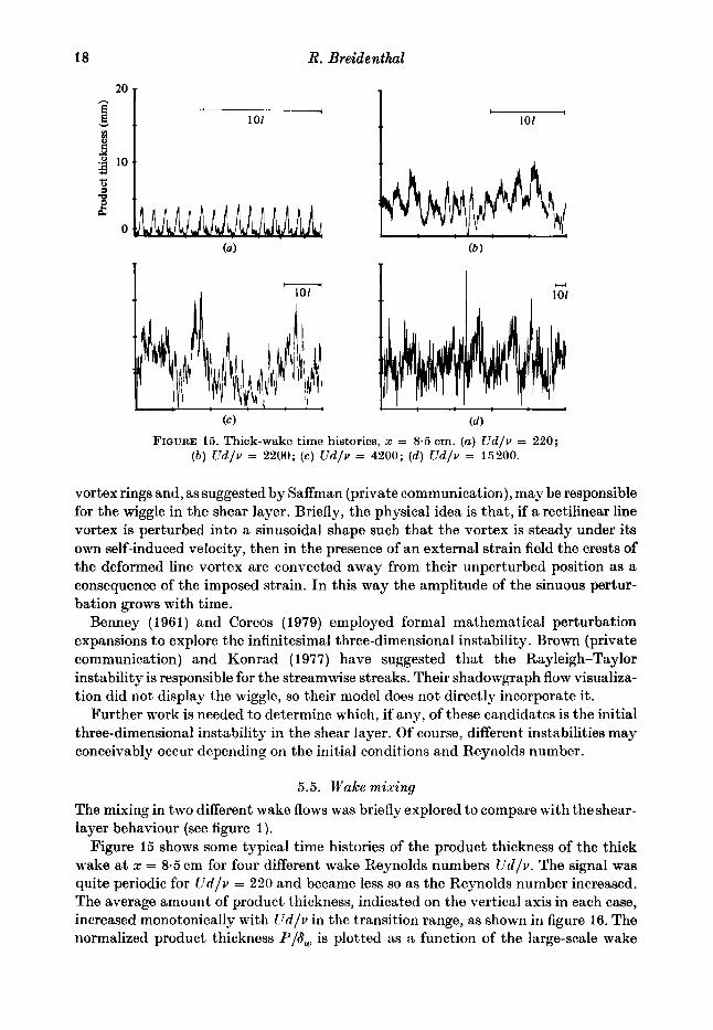
7. Conclusions In summary the effect of Schmidt number on the molecular-scale mixing at low

Reynolds number is pronounced, while at high Reynolds number the mixing changes by only a factor of 2 or less for a three orders of magnitude variation in Schmidt number. Above the transition, the mixing is essentially independent of Re. This is consistent with qualitative predictions of Broadwell’s mixing model. A transition region for the mixing, first observed by Konrad in a gas flow, was again found to correspond to the introduction of small-scale three-dimensional motions into the layer. The aqueous mixing is very sensitive to the presence of these small scales. The large-structure transition Reynolds number was found to vary with velocity ratio, implying that the instability is not a unique function of the large-scale Reynolds number AUS/v as would be the case for the temporal problem of a vortex sheet which is infinitely thin at t = 0. The initial conditions of the finite, laminar vortex sheet leaving the splitter plate are believed to be important in determining the transition. The velocity ratio appears to have relatively small influence on the transition compared to the initial scale and Reynolds number of the higher-speed boundary layer. Further work is necessary to determine the precise shape of the transition curve and its de- pendence on velocity ratio, freestream turbulence, initial vortex-sheet perturbations, spanwise location and other parameters.

The unique flow visualization provided by the chemistry revealed a spanwise- sinuous ‘wiggle ’ which is believed to play an important role in introducing streamwise vortices and small-scale motions in the mixing layer. The initial instability which generates the wiggle is not yet known, although several oandidates exist. The precise evolution of the wiggle and its effect on spanwise variations of the mixing in the mixing layer remain uncertain.

The global structure of other turbulent flows may be fruitfully studied in the future using the reacting flow-visualization technique. The technique complements con- ventional methods using inert tracers since it emphasizes regions of intense mixing. To the extent that these regions correspond to rotational fluid, the reaction product displays the global vorticity.

The author is indebted to Professor Anatol Roshko for his guidance and advice during the course of these experiments. The ideas presented here were developed during discussions with the faculty and students of the Graduate Aeronautioal Laboratory (GALCIT). Most of the wake measurements were done with the help of Till W. Liepmann. The author also wishes to acknowledge the significant contributions of James E. Broadwell, Garry L. Brown, and Anatol Roshko in reviewing the manu- script. The work was made possible by the Air Force Office of Scientific Research under contract F44620-76-C-0046.

Chemical reaction in turbulent mixing layers and wake8 23

P- FIGURE 18. Concentration profiles across a plane reacting interface.

The reaction surface moves to the right with speed v(t ) .

Appendix Phenolphthalein is a pH indicator with a transition interval from about pH = 8

(clear) to pH = 10.5 (red). Half of the phenolphthalein is converted to the red form at pH of 9.3. In order to approximate an irreversible chemical reaction, it is necessary to minimize the disappearance of the red product due to the reverse reaction. This was done by using an excess of OH- in the alkaline stream. The temporal problem of a plane reaction interface is sketched below.

Consider for the moment the diffusion-limited irreversible reaction

A+B+C.

A t t = 0 a membrane disappears separating two half-spaces, the left one containing a uniform concentration of A and the right one uniform with reactant B. For t > 0, the concentration profiles of the reactants and product are error functions. If the equi- valence ratio f = [A],/[B], is unity, then the reaction surface is stationary. In the case of an excess of reactant A, however, Marble & Broadwell (1977) show that the surface moves to the right (see figure 18) with respect to the fluid a t a speed

9 * f-1 f + l '

v( t ) = a (7) , where erf a = -

For f 2 10, v(t) N ( 9 / t ) * . Product is formed at the reaction surface and tencls to be left behind in a region of increasing reactant A as the surface moves to the right.

In the phenolphthalein system we can force the bulk of the red product to be left behind in a region of increasing pH by using an excess of OH- reactant. The red product will thus tend to remain red and not revert back int.0 t,he c~lourless reactants. In practice the amount of excess OH- reactant is limited by a separate reaction which causes the red form to disappear for pH > 12. A pH value of about 11.7 was selected as a compromise.

24 R. Breidenthal

R E F E R E N C E S

BATCHELOR, G. K. 1959 Small scalc variation of convected quantities like temperature in a turbulent fluid. Part I. J . Fluid Mech. 5 , 113.

BATCHELOR, G. K. 1969 Computation of tho energy spectrum in homogcneous 2-D turbulence. Phys. Fluids Suppl. 12, I1 233.

BERNAL, L. P., BREIDENTHAL, R. E., BROWN, G. L., KONRAD, J. H. L ROSHKO, A. 1979 On tho development of three-dimensional small scales in turbulent mixing layers. 2nd Symp. on Turbulent Shear Flows, Imperial College, London.

BENNEY, D. J. 1961 A non-linear theory for oscillations in a parallel flow. J . Fluid Mech. 10, 209.

BRADSHAW, P. 1966 The effect of initial conditions on the development of a frec shear layer. J . Fluid Mech. 26, 225.

BREIDENTHAL, R. E. 1979 Chemically reacting, turbulent shear layer, A.I .A.A. J . 17,310-311. (Also Ph.D. thesis, California Institute of Technology, 1978.)

BROWN, G. L. & ROSHKO, A. 1974 On density effects and large structure in turbulent mixing layers. J . Fluid Mech. 64, 775.

CALDIN, E. F. 1964 Fast Reactions in Solutioki, pp. 66-67. Wiley. CORCOS, G. M. 1979 The mixing layer: deterministic models of a turbulent flow. Univ. Cali-

CZERLINSKI, G. & EICEN, M. 1959 Eine Tcmperaturesprungmethode zur Untersuchung

DIMOTAKIS, P. E. & BROWN, G. L. 1976 The mixing layer at high Reynolds numbor: large-

JIMENEZ, J., MARTINEZ-VAL, R. & REBOLLO, M. 1979 The spectrum of large-scale structures in

KOLTOFF, I. M. 1937 Acid-Base Indicators, p. 221. Macmillan. KONRAD, J. H. 1977 An experimental investigation of mixing in two-dimensional turbulent

shear flows with applications to diffusion-limited chemical reactions. Ph.D. thesis, Cali- fornia Institutc of Technology. (Also Project SQUID Tech. Rep. CIT-8-PU, December 1976.)

MARBLE, F. E. & BROADWELL, J. E. 1977 The coherent flame model for turbulent chemical reactions. TRW Rep. 29314-6001-RE-00.

MOORE, D. W. & SAFFMAN, P. G. 1975 The instability of a straight vortex filament in a strain field. Proc. Roy. SOC. A 346, 413.

ROSHKO, A. 1976 Structure and turbulent shear flows: a new look. A.I .A.A. J . 76-78, Dyden Research Lecture. (Also A.I .A.A. J . 14, 1349-1357).

SAFFMAN, P. G. 1978 The number of waves on unstable vortex rings. J . Fluid Mech. 84, 625. TOOR, H. L. 1962 Mass transfer in dilute turbulent and non-turbulent systems with rapid

irreversible reactions and equal diffusivities, A.I.Ch.E. Journal 8 , no. 1, 70. TSAI, C.-Y. & WIDNALL, S. E. 1976 The stability of short waves on a straight vortex filament

iu a weak externally imposed strain field, J . Fluid Mech. 73, 721. WEDDELL, D. 1941 Turbulent mixing in gar flames, p. 115. Ph.D. thesis, Maasachusetts Institute

of Technology. WIDNALL, Y. E., BLISS, D. B. BE TSAI, C.-Y. 1974 The instability of short waves on a vortex

ring. J . Fluid Mech. 66, 35. WINANT, C. D. & BROWAND, F. K. 1974 Vortex pairing: the mechanism of turbulent mixing

layer growth at moderate Reynolds number. J . Fluid Mech. 63,237. WITTE, A. B., BROADWELL, J .E. , SHACKLEFORD, W. L., CUMMINCS, J.C., TROST, J. E.,

WHITEMAN, A. S., MARBLE, F. E., CRAWFORD, D. R. & JACOBS, T. A. 1974 Aerodynamic reactive flow studies of the H,F, laser-11. Air Force Weapon8 Lab., Kirtland Air Force Baee, New Mexico, AFWL-TE-74-78, 33.

WYGNANSKI, I., OSTER, D. & FIEDLER, H. 1979 The forced, plane, turbulent mixing layer: a challenge for the predictor. 2nd Symp. on Turbulent Shear Flows, Imperial College, Londoir, p. 8.12.

forttia, Berkeley, Rep. FM-79-2.

chemischcr Relaxation. 2. Electrochemie 63 (6), 652.

structure dynamics and entrainment. J . Fluid Mech. 78, 535.

a mixing layer. 2nd Symp. on Turbulmt Shear Flows, Imperial College, Londolt, p. 8.7.