Structure and function of small, headwater streams flowing ...

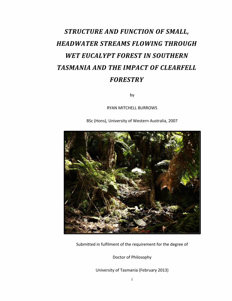
i

STRUCTURE AND FUNCTION OF SMALL,

HEADWATER STREAMS FLOWING THROUGH

WET EUCALYPT FOREST IN SOUTHERN

TASMANIA AND THE IMPACT OF CLEARFELL

FORESTRY

by

RYAN MITCHELL BURROWS

BSc (Hons), University of Western Australia, 2007

Submitted in fulfilment of the requirement for the degree of

Doctor of Philosophy

University of Tasmania (February 2013)

iii

Declaration of originality

I hereby declare that this thesis contains no material which has been accepted for a

degree or diploma by the University or any other institution, except by way of

background information and duly acknowledged in the thesis, and to the best of my

knowledge and belief no material previously published or written by another person

except where due acknowledgement is made in the text of the thesis, nor does the

thesis contain any material that infringes copyright.

5th February 2013

Ryan Burrows Date

Authority of access

This thesis may be made available for loan and limited copying and communication

in accordance with the Copyright Act 1968.

Statement regarding published work contained in this thesis

The publishers of the papers comprising Chapters 2 to 4 hold the copyright for that

content, and access to the material should be sought from the respective journals.

The remaining non published content of the thesis may be made available for loan

and limited copying and communication in accordance with the Copyright Act 1968.

5th February 2013

Ryan Burrows Date

iv

Statement of publications

Manuscripts (published or submitted to peer-reviewed journals) produced as part of

this thesis:

(1) Burrows, R. M., Magierowski, R. H., Fellman, J. B., and Barmuta, L. A. 2012,

Woody debris input and function in old-growth and clear-felled headwater

streams. Forest Ecology and Management, 286: 73-80.

(2) Burrows, R. M., Fellman, J. B., Magierowski, R. H., and Barmuta, L. A. 2013,

Greater phosphorus uptake in forested headwater streams modified by

clearfell forestry. Hydrobiologia, 703: 1-14.

(3) Burrows, R. M., Fellman, J. B., Magierowski, R. H., and Barmuta, L. A. 2013,

Allochthonous dissolved organic matter controls bacterial carbon production

in old-growth and clearfelled headwater streams. Freshwater Science, 32(3):

DOI: 10.1899/12-163.

Statement of Co-Authorship

The following people and institutions contributed to the publication of work

undertaken as part of this thesis:

Ryan M. Burrows (University of Tasmania) was the lead author of the three papers

and contributed to all aspects of each study including the development of ideas, the

collection and analysis of data, and the writing of the manuscript.

Leon A. Barmuta (University of Tasmania) assisted with guidance and supervision of

the research relating to the development of ideas, data collection, statistical

analysis, interpretation of results, and producing publishable manuscripts of (1), (2),

and (3).

Regina H. Magierowski (University of Tasmania) assisted with guidance and

supervision of the research relating to the development of ideas, data collection,

v

statistical analysis, interpretation of results, and producing publishable manuscripts

of (1), (2), and (3).

Jason B. Fellman (University of Western Australia and University of Alaska

Southeast) assisted with guidance and supervision of the research relating to the

data preparation, statistical analysis, interpretation of results, and producing

publishable manuscripts of (1), (2), and (3).

We, the undersigned, agree with the above stated “proportion of work undertaken”

for each of the above published (or submitted) peer-reviewed manuscripts

contributing to this thesis:

Signed: __________________ ______________________

Leon Barmuta Elissa Cameron

Supervisor Head of School

School of Zoology School of Zoology

University of Tasmania University of Tasmania

Date:_____________________ _____________________

vi

Statement of communications

Conference proceedings in which I was the primary presenter as part of this thesis:

Burrows, R. M., Fellman, J. B., Magierowski, R. H., and Barmuta, L. A. 2011,

Increased phosphorus retention in Tasmanian headwater streams modified by

clearfell, burn and sow forestry. Abstracts of the 50th Annual Congress of the

Australian Society of Limnology (ASL) with the New Zealand Freshwater Science

Society (NZFSS), Brisbane, Australia.


Increased phosphorus retention in Tasmanian headwater streams modified by

clearfell, burn and sow forestry. Abstracts of the Ecological Society of Australia

Annual Conference, Hobart, Australia.

Burrows, R. M., Fellman, J. B., Magierowski, R. H., and Barmuta, L. A. 2012, Greater

phosphorus uptake in forested headwater streams modified by clearfell forestry.

Abstracts of the CRC for Forestry Annual Science Meeting, Sunshine Coast, Australia.

Burrows, R. M., Fellman, J. B., Magierowski, R. H., and Barmuta, L. A. 2012, Greater

phosphorus uptake in forested headwater streams modified by clearfell forestry.

Abstracts of the Society of Freshwater Science Annual Meeting, Louisville, U.S.A.


Allochthonous dissolved organic matter controls bacterial carbon production in

forested, headwater streams. Abstracts of the Tasmanian Australian Society of

Limnology (ASL) Forum, Hobart, Australia.

vii

Abbreviations

AFDM Ash-free dry mass

AICc Akaike’s Information Criterion adjusted for small sample size

ANCOVA Analysis of covariance

ANOSM Analysis of similarity

ANOVA Analysis of variance

BA Before-after

BCP Bacterial carbon production

C Carbon

C1 Component 1

C2 Component 2

C3 Component 3

CBS Clearfell, burn and sow

CDP Cellulose decomposition potential

CI Control-impact

CPOM Coarse particulate organic matter

CTFL Cotton tensile force loss

CTFR Cotton tensile force ratio

DIN Dissolved inorganic nitrogen

DOC Dissolved organic carbon

DOM Dissolved organic matter

DON Dissolved organic nitrogen

DOP Dissolved organic phosphorus

EEMs Excitation-emission matrices

FI Fluorescence index

FPOM Fine particulate organic mater

FWD Fine woody debris

GLA Gap Light Analyzer

ha Hectare

HCL Hydrochloric acid

IBRA Interim Biogeographic Regionalisation for Australia

LAI Leaf area index

LMM Linear mixed-effects model

LWD Large woody debris

m asl Meters above sea level

MBACI Multiple before-after control-impact

MEZ Machinery exclusion zone

N Nitrogen

NH3 Nitrate

NH4 Ammonium

nMDS Non-metric multidimensional scaling

viii

OG Old-growth

OM Organic matter

P Phosphorus

PARAFAC Parallel factor analysis

PERMANOVA Permutational multivariate analysis of variance

PERMDISP Permutational analysis of multivariate dispersions

SRP Soluable reactive phosphorus

SUVA Specific ultra-violet absorbance

Sw Uptake length

TCA Trichloroacetic acid

TDN Total dissolved nitrogen

TN Total nitrogen

TOC Total organic carbon

TP Total phosphorus

TSH Time since harvest

TSR Tasmanian Southern Ranges

Uf Uptake rate

UV Ultra-violet

UVA Ultra-violet radiation

Vf Uptake velocity

VIS Visable

Wt Weight

ix

Acknowledgments

First and foremost I would like to thank my supervisors, Associate Professor Leon

Barmuta and Dr. Regina Magierowski, for their support and guidance over the years.

Without your energy and enthusiasm for freshwater ecosystems this project would

not have been possible. I would also like to thank my research advisor, Dr. Jason

Fellman, who has provided advice and guidance from afar in both Western Australia

and Alaska. The words in this thesis are just a fraction of the knowledge that you

have all shared with me, but they have culminated into this body of work which I am

very proud of.

Thanks to Chris Spencer from the Tasmanian Forest Practices Authority (FPA) for the

many weeks spent in the field with me. Your local knowledge of Tasmanian flora

and fauna, forest practices, and leach removal was invaluable. Thank you to Dr. Jean

Jackson for teaching me how to operate the study weirs and insert cotton strips into

benthic sediment. Thanks also to Dr. Joanne Clapcott for your role in initiating the

MBACI headwater streams project and to Laurie Cook for collecting the data when

no one else could.

A special thanks for all those volunteers who helped my find study sites, collect

water samples, measure woody debris, and conduct experiments: K. Hawkes, J.

Delaine, E. Polymeropoulos, T. Hollings, J. Haag, J. Fountain, S. Griffin, A. Brüniche-

Olsen, J. Kramer, J. Goon, K. Kreger, M. Burrows, B. Burrows, A. Watson, and L.

Quayle. Without your help through rain, hail, snow, and sunshine this fieldwork

would not have been possible!

I am indebted to all the Forestry Tasmania staff that assisted me through this

journey. In the Hobart office I’d like to thank Dr. Sandra Roberts for your feedback

regarding the management implications of my research and Dr. Crispen Marunda

for providing me with the best possible estimates of sub-catchment boundaries. A

huge thanks to all those in the Huon district office, especially Cath and Matt, for

x

providing the right gate keys and ensuring that I was always home safe at the end of

each day.

Thanks to all the staff at FPA who assisted me over the years, including Dr. Sarah

Munks who always provided me with the support that I required. A large part of this

thesis would not have been possible if it was not for the in-kind support of this

organisation.

Thank you to all the staff, academics, and fellow postgraduates at the School of

Zoology who have made me feel welcome and kept my project running like a well-

oiled machine. In particular I’d like to thank Richard Holmes for all the equipment

repairs and ideas; Wayne Kelly for the IT and laboratory support; Kate Hamilton and

Adam Smolenski for the laboratory equipment and support; Adam Stephens and

Simon Talbot for organising vehicles and attempting to unravel the OH&S

procedures of Zoology and UTAS; Barry Rumbold for all the financial thumbs up;

Felicity Wilkinson for simply being the best secretary ever; and Chris Burridge for

the footy tips. I cannot thank my fellow postgraduate students enough for the

support, encouragement, ideas, food, beer, and fun times you have all provided and

shared me.

I would like to thank my Washington and Cartela housemates over the years: Tracey

Hollings, Elias Polymeropoulos, Martin Wæver Pedersen, Judith Fernandez, Lydie

Lescarmontier, Jon DeLaine, Alex Stedman, Bandit, and Steal – I could not have

asked for better friends and hounds!

To my family and friends, thank you for supporting and encouraging me throughout

this adventure. Even though many of you were on other side of the country, none of

this would have been possible without your love and support. Finally, thanks to Kris

for your immense emotional and financial support, patience, encouragement, and

love throughout the years. I cannot guarantee that I won’t still require these after

this thesis is finalised!

xi

This thesis was supported by a range of funding bodies. My Postgraduate

Scholarship was funded by the University of Tasmania, School of Zoology, and the

CRC for Forestry. Financial support for research included: a Student Grant from the

Tasmanian Forest Practices Authority; Holsworth Wildlife Research Endowment;

Maxwell Ralph Jacobs Fund of The Institute of Foresters of Australia; and a Warra

Grant from Forestry Tasmania. In-kind support was provided by FPA and Forestry

Tasmania. I sincerely thank all of you for your generous contributions.

Holsworth Wildlife Research Endowment

xii

Abstract

Clearfell, burn and sow (CBS) forestry is a major disturbance to headwater

streams flowing through wet eucalypt forests in southern Tasmania involving

clearfelling trees around them and the burning of remaining slash within a year of

harvest. The aim of this research was to assess the short-term (<19 years) effects of

CBS forestry on several key structural (woody debris and dissolved organic matter

source and composition) and functional (nutrient uptake and organic matter

processing) characteristics of headwater streams in southern Tasmania. I evaluated

these using a combination of replicated space-for-time surveys and an MBACI

(multiple before-after control-impact) experiment in headwater stream reaches

flowing through old-growth and CBS-affected forest.

My findings show that CBS forestry increased available light, elevated water

temperatures (between 0.25 and 0.94°C), and significantly increased the quantity of

woody debris situated in the stream channel. I also used fluorescence

characterisation of dissolved organic matter (DOM) to show that forest harvesting

did not affect the relative contributions of autochthonous and allochthonous stream

DOM despite the major reach-scale disturbance that clearfell forestry represents.

However, there was conflicting evidence for changes in DOM composition after

harvesting. It is likely that catchment-scale processes are more important than

reach-scale processes (i.e. forest harvesting) in determining stream DOM

biogeochemistry, because only a small proportion of the total channel length (<100

m) is affected by clearfell forestry.

The large physical structural changes to headwater streams caused by CBS

forestry led to changes in stream function. Nutrient addition experiments showed

greater phosphorus uptake in CBS-affected relative to old-growth (OG) stream

reaches, which was likely due to increased biotic activity (algae and bacterial

biofilms) related to greater in-stream light availability and quantity of in-stream

xiii

woody debris. However, sorption to sediment and charred woody debris may also

have contributed to the greater phosphorus uptake after harvesting. The impact of

CBS forestry on organic matter decomposition differed among years and benthic

habitats, with evidence for an increase in bacterial carbon production (BCP) in fine

sediment habitat but a decrease in BCP and cellulose decomposition in coarse gravel

habitat. Contrary to most previous research, increasing contribution of terrestrial

DOM was the strongest variable driving in situ benthic BCP.

Some of the structural changes from CBS may be beneficial in reducing

impacts at the catchment-scale. For instance, the observed increase in the amount

of woody debris and light availability after harvesting may prevent elevated

phosphorus export to downstream ecosystems by increasing phosphorus uptake

and retention in headwaters. While these effects characterised the short-term

responses to CBS in these headwater streams, the longer-term (>19 years) and

catchment-scale impacts require further research. Many variables (e.g. the quantity

of woody debris) will take decades to recover to pre-disturbance levels and the

cumulative impacts of harvesting multiple coupes throughout the landscape needs

to be determined to ensure that CBS operations are managed in space and time to

minimise impacts on downstream ecosystems.

xiv

Table of Contents

Abbreviations .............................................................................................................. vii

Acknowledgments ........................................................................................................ ix

Abstract ................................................................................................................. xii

Table of Contents ....................................................................................................... xiv

List of Figures ............................................................................................................ xviii

List of Tables ............................................................................................................. xxiii

Chapter 1. General Introduction ................................................................................ 1

Freshwater ecosystems and anthropogenic disturbance ........................................ 2

1.1. Assessing disturbance in streams and rivers ........................................ 3

1.2. Headwater streams ............................................................................... 4

1.3. Impact of forest harvesting on headwater streams ............................. 9

1.4. Tasmanian headwater streams and clearfell, burn and sow (CBS) forestry ................................................................................................ 10

1.5. Contributing to the understanding of how disturbance influences the structure and function of headwater streams ................................... 14

1.6. Thesis aims .......................................................................................... 15

Chapter 2. Woody debris input and function in old-growth and clearfelled headwater streams ................................................................................. 19

2.1. Abstract ............................................................................................... 20

2.2. Introduction ........................................................................................ 20

2.3. Methods .............................................................................................. 23

2.3.1. Study region and streams ............................................................... 23

2.3.2. Field procedures .............................................................................. 27

2.3.3. Data analysis .................................................................................... 30

2.4. Results ................................................................................................. 31

2.4.1. Woody debris abundance and volume ........................................... 31

2.4.2. Woody debris function and decay class .......................................... 32

2.5. Discussion ........................................................................................... 37

2.5.1. Response of woody debris abundance and volume to CBS forestry ......................................................................................................... 37

2.5.2. Greater functional role of woody debris in CBS-affected streams . 37

xv

2.5.3. More decayed woody debris in OG than CBS-affected streams..... 38

2.5.4. Longer-term legacies ....................................................................... 39

2.5.5. Implications for forest management .............................................. 40

2.6. Acknowledgments .............................................................................. 40

2.7. Role of the funding source .................................................................. 41

Chapter 3. Greater phosphorus uptake in forested headwater streams modified by clearfell forestry ..................................................................................... 43

3.1. Abstract ............................................................................................... 44

3.2. Introduction ........................................................................................ 44

3.3. Methods .............................................................................................. 47

3.3.1. Study region .................................................................................... 47

3.3.2. Stream reaches ................................................................................ 49

3.3.3. Environmental variables.................................................................. 51

3.3.4. Nutrient addition experiment ......................................................... 52

3.3.5. Laboratory analysis ......................................................................... 53

3.3.6. Nutrient spiralling metrics .............................................................. 54

3.3.7. Data analysis .................................................................................... 54

3.4. Results ................................................................................................. 56

3.4.1. Environmental characteristics ......................................................... 56

3.4.2. Nutrient uptake metrics .................................................................. 56

3.4.3. Relationships between uptake metrics and environmental variables ......................................................................................................... 59

3.5. Discussion ........................................................................................... 59

3.5.1. Nutrient retention in CBS-affected and old growth reaches .......... 59

3.5.2. Patterns of stream nutrient uptake after disturbance ................... 63

3.5.3. Catchment-scale implications ......................................................... 64


Chapter 4. Allochthonous dissolved organic matter controls bacterial carbon production in old-growth and clearfelled headwater streams .............. 67

4.1. Abstract ............................................................................................... 68

4.2. Introduction ........................................................................................ 68

4.3. Methods .............................................................................................. 71


xvi

4.3.2. Field sampling.................................................................................. 73

4.3.3. Laboratory procedures .................................................................... 75

4.3.4. Calculations and statistical analyses ............................................... 77

4.3.4.1. Spectroscopic analyses and PARAFAC modelling ...................................... 77

4.3.4.2. Impact of CBS forestry on DOM and environmental variables ................. 78

4.3.4.3. Relationships of variables with BCP .......................................................... 79

4.4. Results ................................................................................................. 80

4.4.1. BCP and environmental variables ................................................... 80

4.4.2. Fluorescence index and SUVA254 ..................................................... 81

4.4.3. EEM – PARAFAC............................................................................... 84

4.4.4. Relationships of BCP with environmental and DOM variables. ...... 87

4.5. Discussion ........................................................................................... 89

4.5.1. BCP relationships with environmental and DOM variables ............ 89

4.5.2. Forest harvesting influence on DOM source and composition ...... 92

4.5.3. Catchment-scale implications ......................................................... 93


Chapter 5. Effect of clearfell harvesting on organic matter decomposition differs among benthic habitats in forested, headwater streams ...................... 95

5.1. Abstract ............................................................................................... 96

5.2. Introduction ........................................................................................ 96

5.3. Methods .............................................................................................. 99


5.3.2. Field procedures ............................................................................ 103

5.3.2.1. Organic matter decomposition ............................................................... 103

5.3.2.2. Environmental variables .......................................................................... 104

5.3.3. Laboratory procedures .................................................................. 105

5.3.4. Data analysis .................................................................................. 107

5.3.4.1. Data preparation ..................................................................................... 107

5.3.4.2. Assessing the response of temperature and OM decomposition to CBS forestry ................................................................................................ 107

5.4. Results ............................................................................................... 113

5.4.1. Stream environmental characteristics .......................................... 113

5.4.2. Temperature response to CBS forestry ......................................... 116

5.4.3. Response of cotton strip decomposition to CBS forestry ............. 118

xvii

5.4.4. Response of bacterial carbon production to CBS forestry ............ 122

5.5. Discussion ......................................................................................... 126

5.5.1. Elevated water temperature after CBS forestry ........................... 126

5.5.2. Contrasting response of OM decomposition to CBS forestry ....... 127

5.5.3. Cotton strips and BCP assays as reach-scale bio-indicators of stream perturbation .................................................................................. 130

5.5.4. Catchment implications ................................................................ 131

5.5.5. Forest management implications ................................................. 133

5.6. Acknowledgements........................................................................... 134

5.7. Appendix ........................................................................................... 136

Chapter 6. General discussion ................................................................................ 141

6.1. Synthesis - The effect of CBS forestry on the structure and function of southern Tasmanian headwater streams ......................................... 142

6.2. Context: how does CBS forestry compare to other disturbances in wet eucalypt forests of southern Tasmania? .......................................... 150

6.2.1. Storm damage ............................................................................... 150

6.2.2. Superb lyrebirds ............................................................................ 151

6.2.3. Wildfire .......................................................................................... 153

6.3. Paradigms for assessing disturbance ................................................ 155

6.3.1. Resistance and resilience of individual stream variables to CBS forestry .......................................................................................... 156

6.3.2. Stream ecological integrity ........................................................... 160

6.4. Management implications ................................................................ 160

6.5. Future directions ............................................................................... 162

Chapter 7. References ............................................................................................ 165

xviii

List of Figures

Figure 1.1. A schematic representation of an upland catchment showing the drainage divide (dashed black line) with stream channels labelled using the Strahler channel ordering system. ................................................................. 5

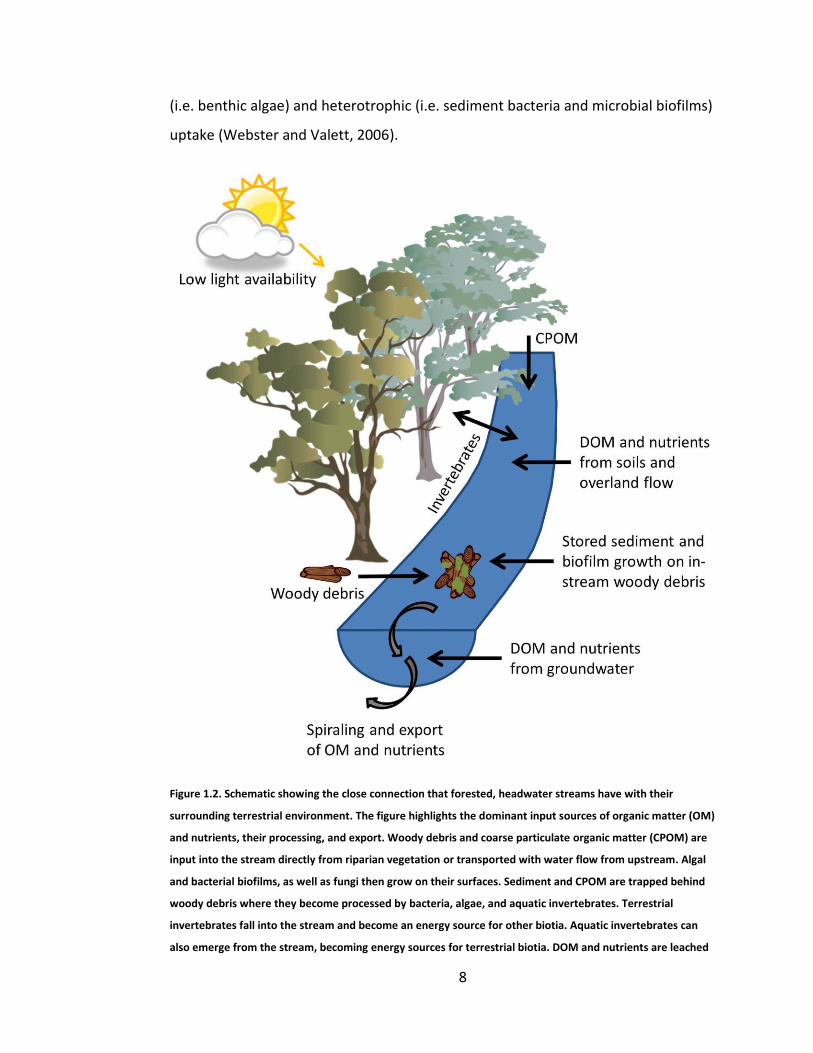
Figure 1.2. Schematic showing the close connection that forested, headwater streams have with their surrounding terrestrial environment. The figure highlights the dominant input sources of organic matter (OM) and nutrients, their processing, and export. Woody debris and coarse particulate organic matter (CPOM) are input into the stream directly from riparian vegetation or transported with water flow from upstream. Algal and bacterial biofilms, as well as fungi then grow on their surfaces. Sediment and CPOM are trapped behind woody debris where they become processed by bacteria, algae, and aquatic invertebrates. Terrestrial invertebrates fall into the stream and become an energy source for other biotia. Aquatic invertebrates can also emerge from the stream, becoming energy sources for terrestrial biotia. DOM and nutrients are leached from terrestrial OM and soils or input via groundwater recharge. The uptake and cycling of OM and nutrients occurs while they are being continuously transported downstream. This illustration has been adapted from Richard and Danehy (2007). ........................................................................................ 8

Figure 1.3. The riparian protection from CBS forestry provided to different size streams in Tasmania. Class 4 streams refer to 1st order headwater streams. Source: Tasmanian Forest Practices Code (2002). ....................................... 12

Figure 1.4. A picture of scorched vegetation within a machinery exclusion zone (MEZ) of a headwater stream flowing through a CBS-affected coupe (<1 year since harvesting) in southern Tasmania. ............................................. 12

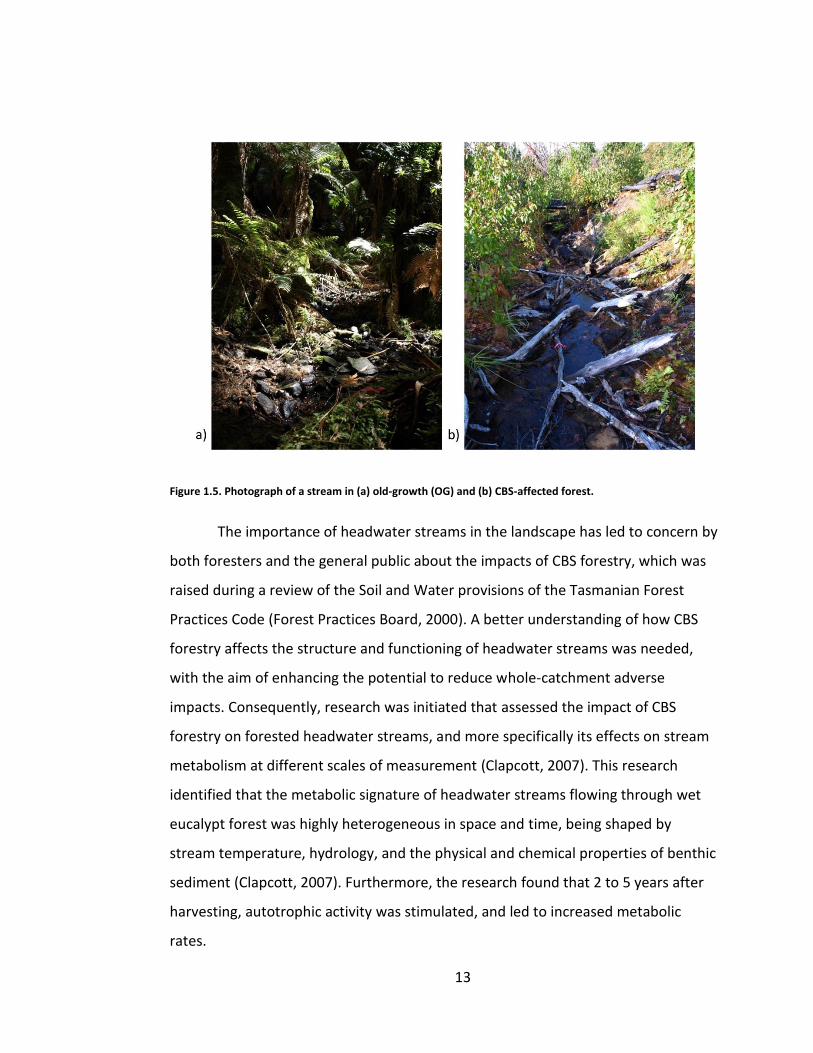
Figure 1.5. Photograph of a stream in (a) old-growth (OG) and (b) CBS-affected forest. ........................................................................................................... 13

Figure 2.1. The location of five old-growth (OG; solid circles) and five CBS-affected (white circles) stream reaches in southern Tasmania. Only larger streams and rivers (solid lines) are shown because lower order (1 - 4) streams are simply too abundant in the region and have not been accurately mapped. ...................................................................................................................... 25

Figure 2.2. Illustration of the woody debris survey design. The entire stream reaches was surveyed for old-growth (OG) stream reaches. However, for CBS-affected reaches only 1 m either side (white rectangle) of each survey point (dashed line), including the start and finish, was surveyed. .............. 27

Figure 2.3. The proportion of FWD and LWD in each function class for CBS-affected (grey) and old-growth (white) stream reaches. The function classes are: AB

xix

- Armouring bank; BI – Biological interaction; FP – Forming pools; NF – No function; PS – Providing substrate; SF – Step formation; SS – Storing sediment; SW – Storing wood. Different letters above the bars indicate significant differences (Chi-square tests with a sharpened-False Discovery Rate (FDR) correction; P < 0.05) among function classes. ........................... 35

Figure 2.4. The average (± standard error) decay class of FWD and LWD in each position class for CBS-affected (grey) and old-growth stream reaches. Different letters above the bars indicate significant differences (ANOVA; P < 0.05) between disturbance categories among position classes. ................. 36

Figure 3.1. Map of the four old growth (OG; filled triangle) and three CBS-affected (CBS; filled circle) stream reaches in southern Tasmania. First-order headwater streams (including my study streams) are not mapped for this region. Base data (larger stream network) by CFEV, © State of Tasmania (CFEV database v1.0, 2005). ......................................................................... 48

Figure 3.2. A non-metric MDS representing the Euclidean distance among four old growth (filled triangle) and three CBS-affected (filled circle) stream reaches based on normalised environmental variables. The predictor environmental variables that contributed most to the average dissimilarity between CBS-affected and OG stream reaches in the SIMPER analysis are overlaid. These environmental variables include: leaf area index (LAI; m2/m2), the volume of FWD per square metre of wetted-bank surface area (VFWD; m3 m-2), the number of FWD pieces per metre of stream reach (FWD; pieces m-1), and the number of LWD pieces per metre of stream reach (LWD; pieces m-1). 57

Figure 3.3. The average values of uptake length (Sw; m), uptake velocity (Vf; mm min-1), and uptake rate (U; µg mm min-1) of ammonium (NH4; A- C) and soluble reactive phosphorus (SRP; D- F) for old growth (OG) and CBS-affected (CBS) stream reaches in the wet eucalypt forest of southern Tasmania. The bootstrapped 95% confidence intervals of the mean are given. ............................................................................................................ 58

Figure 3.4. Relationship of the uptake velocity (Vf) of SRP and (A) the number of FWD pieces per metre of stream reach (pieces m-1), (B) volume of FWD per square metre of wetted-bank surface area (m3 m-2), (C) leaf area index (LAI; m2/m2), (D) the particle size variability of fine sediment (µm; D90D10) for old growth (OG; filled triangle) and CBS-affected (CBS; filled circle) streams. The stream reach names are displayed in (A). The R2 and P value from linear regressions between Vf(SRP) and each variable are also displayed. .............. 60

Figure 4.1. Locations of 3 old-growth (OG) and seventeen clearfell, burn, and sow (CBS) affected stream reaches in southern Tasmania. Only larger streams and rivers are shown because smaller streams (1st-to 3rd-order) are too abundant in the region and have not been accurately mapped. ................ 72

xx

Figure 4.2. Spectral characteristics of the 3 parallel factor analysis (PARAFAC) components (A) and the split-half analysis of each component (B). S1 and S2 indicate each half of the data set in the split-half analysis. Intensities are in Raman units. Ex = excitation, Em = emission, C1 = Component 1, C2 = Component 2, and C3 = Component 3. ........................................................ 78

Figure 4.3. Box-and-whisker plots for bacterial C production (BCP) (A), NH4 (B), NO3 (C), total dissolved N (TDN) (D), sediment total N (TN) (E), and sediment total P (TP) (F) at 20 study streams in Tasmania. Dotted lines in boxes are means, solid lines in boxes are medians, box ends are 25th and 75th quartiles, whiskers show maximum and minimum values, and dots show outliers. ........................................................................................................ 82

Figure 4.4. Box-and-whisker plots for sediment total organic C (TOC) (A), dissolved organic C (DOC) (B), dissolved organic N (DON) (C), chlorophyll a (D), fluorescence index (FI) (E), and specific UV absorbance (SUVA254) (F) at 20 study streams in Tasmania. Dotted lines in boxes are means, solid lines in boxes are medians, box ends are 25th and 75th quartiles, whiskers show maximum and minimum values, and dots show outliers. ........................... 83

Figure 4.5. The relationship between the time since harvest (TSH) and the relative abundance (%Fmax) of humic-like component (C1) (A), fulvic like component (C2) (B), and protein like component (C3) (C). The relative proportions of parallel factor (PARAFAC) components for old-growth (OG) streams also are displayed. A line of best fit for the regression is overlaid. The slopes of the lines of best fit were not significantly different from 0 (R2 ≤ 0.1, P ≥ 0.1). ............................................................................................... 86

Figure 4.6. The relationships between benthic bacterial C production (BCP) and the fluorescence index (FI) of stream water modelled with linear regression (A), FI modelled with polynomial regression (B), and benthic sediment total N (TN) (C). Curves of best fit are overlaid with 95% confidence intervals. ..... 88

Figure 5.1. Map of the seven study streams in southern Tasmania labelled streams A, B, and D to H. Only higher order streams (> 4) and rivers are shown. .. 101

Figure 5.2. Photograph of the tensiometer used to measure the tensile strength of cotton strips. .............................................................................................. 105

Figure 5.3. Flow chart showing the decisions and sequence of tests used to assess whether there was evidence for a significant change in OM decomposition after clearfell, burn, and sow (CBS) operations. ........................................ 110

Figure 5.4. Average daily stream discharges (Q; L sec-1) for each of the seven study streams between 2004 and 2012. Gaps in the data exist were data could not be estimated with linear regression due to failure of water level loggers. ....................................................................................................... 114

xxi

Figure 5.5. Average daily stream temperatures (°C) for each of the seven study streams between 2004 and 2012. Gaps in the data exist due to failure of temperature loggers. Vertical lines represent the harvest (red) and burn (brown) dates for harvested streams. ....................................................... 115

Figure 5.6. Average cotton strip force ratio (CSFR) in coarse gravel sediment for each of the seven study streams in each sampling occasion between 2004 and 2012. Vertical lines represent the harvest (red) and burn (brown) dates for impacted streams. CSFR sampling dates not subject to harvesting are represented by a solid circle (control; c) and those after harvesting are represented by a different symbol for each year after CBS forestry. ........ 119

Figure 5.7. Average cotton strip force ratio (CSFR) in fine sediment for each of the seven study streams in each sampling occasion between 2004 and 2012. Vertical lines represent the harvest (red) and burn (brown) dates for impacted streams. CSFR sampling dates subject to no harvesting are represented by a solid circle and those after harvesting are represented by a different symbol for each year after CBS forestry. ................................. 120

Figure 5.8. The linear relationship between benthic cotton strip force ratio and sediment temperature in a) fine sediment and b) coarse gravel habitat. A line of best fit is overlaid (solid blue line). ................................................. 122

Figure 5.9. Average BCP in coarse gravel sediment for each of the seven study streams in each sampling occasion between 2004 and 2012. Vertical lines represent the harvest (red) and burn (brown) dates for impacted streams. BCP sampling dates subject to no harvesting are represented by a solid circle and those after harvesting are represented by a different symbol for each year after CBS forestry....................................................................... 123

Figure 5.10. Average BCP in fine sediment for each of the seven study streams in each sampling occasion between 2004 and 2012. Vertical lines represent the harvest (red) and burn (brown) dates for impacted streams. BCP sampling dates subject to no harvesting are represented by a solid circle and those after harvesting are represented by a different symbol for each year after CBS forestry. .............................................................................. 124

Figure 5.11. The linear relationship between benthic bacterial carbon production (BCP; mg C m-2 d-1) and sediment temperature in a) fine sediment and b) coarse gravel habitat. A line of best fit is overlaid (solid blue line). .......... 126

Figure 6.1. Schematic of the response effect size of the measured stream variables in my thesis to CBS forestry (0 to 19 years after CBS), relative to reference conditions. Arrows represents the time of CBS forestry. Solid lines denote actual data (significant or not) while dotted lines denote the predicted response. .................................................................................................... 143

xxii

Figure 6.2. Schematic showing the changes to the physical and chemical structure of small, headwater streams in southern Tasmania after CBS forestry. This illustration has been adapted from Richard and Danehy (2007)............... 146

Figure 6.3. Schematic showing the likely short-term (<19 years) interactions between changes to the structure (left of stream) and function (right of stream) of small, headwater streams in southern Tasmania immediately after CBS operations. Arrows represent the direction of the response of that variable after CBS operations (yellow arrow = increase, red arrow = decrease). The hollow tilde symbol represents no change in that variable after CBS operations. ................................................................................. 149

Figure 6.4. Photograph of a tree that has fallen directly over a headwater stream in southern Tasmania. .................................................................................... 151

Figure 6.5. A photograph of a southern Tasmanian headwater stream with evidence of superb lyrebird (Menura novaehllandiae) activity (white outlined area). .................................................................................................................... 153

Figure 6.6. A conceptual diagram showing the difference in the frequency of woody debris input between headwater streams affected by wildfire (a) and (b) harvesting. .................................................................................................. 155

xxiii

List of Tables

Table 2.1. The geographical coordinates, environmental, and morphological characteristics of the ten study sites. Stream width and depth values are averages ± standard error. NA means ‘not applicable’. Stream channel width, wetted channel width, and depth are for base flow conditions. ..... 26

Table 2.2. The description of the categories used to measure the function, decay, and position class of FWD and LWD. ........................................................... 29

Table 2.3. The P-values from the permutational multivariate analysis of variance which tested whether the volume and abundance of FWD and LWD (expressed m-1 of surveyed channel length and m-2 of stream wetted-bank channel) were significantly different between CBS-affected and OG stream reaches. Listed below these P-values are the position classes which were found to be significant discriminators at P < 0.05 of the difference in volume and abundance between CBS-affected and OG stream reaches. ... 32

Table 2.4. The average ± standard error of the abundance and volume (expressed m-

1 and m-2 of stream channel) of FWD and LWD located in-stream and above the stream. The P-value for the ANOVA and ANOVA analyses are shown. 34

Table 3.1. Stream reach characteristics, and ambient water chemistry for the old growth (OG) and clearfell, burn and sow (CBS) affected study streams. NA refers to those streams that have no history of forestry disturbance. Standard errors are shown for the mean water depth and mean stream width. NH4 and SRP enrichment refers to the nutrient concentration at which stream water was elevated above ambient levels during each experiment. .................................................................................................. 50

Table 3.2. The output from a SIMPER (PRIMER5) analysis that was used to identify the environmental variables that contributed most to the average dissimilarity between CBS-affected and OG stream reaches. The metrics presented in the table are the average dissimilarity value (Av. value), standard deviation (Std. dev.), the ratio of the average dissimilarity to standard deviation (SIM/SD), and the percent contribution of each normalised variable to the average dissimilarity between CBS-affected and OG stream reaches. Environmental variables are significant if they contributed ≥5% to the average dissimilarity between reach types and had a ratio of the average dissimilarity to standard deviation ≥1.4. Only the first six variables are displayed. ........................................................................... 57

Table 4.1. Physical characteristics of 20 bacterial carbon production (BCP) study streams in Tasmania. LAI = leaf area index. NA refers to streams that have no history of forestry disturbance. .............................................................. 73

xxiv

Table 4.2. Candidate models used in the AICc model selection with BCP as the response variable. K indicates the number of model parameters. Variables include stream temperature, sediment total N (TN), fluorescence index (FI), and FI fitted with a 2nd-order polynomial (FI2). .......................................... 80

Table 4.3. The excitation and emission maximum, relative abundance (% Fmax) of fluorescent components in the twenty BCP study streams, parallel factor (PARAFAC) component references, and description of each component from the 3-component PARAFAC model. 1 Coble (1996); 2 Williams et al. (2010); 3 Stedmon and Markager (2005); 4 Cory and McKnight (2005); 5 Murphy et al. (2006); 6 Fellman et al. (2008). UVA = ultraviolet A. ............. 85

Table 4.4. The slope, R2, and p-values from the simple linear regression between bacterial C production (BCP) and the environmental and dissolved organic matter (DOM) variables in 20 study streams in Tasmania. LAI = leaf area index, DOC = dissolved organic C, SUVA254 = specific ultraviolet absorbance of DOM, TDN = total dissolved N, DON = dissolved organic N, TN = total N, TP = total P, AFDM = ash-free dry-mass, TOC = total organic C, FI = fluorescence index, C1–3 = parallel factor components.............................. 87

Table 4.5. The model number (Table 4.2), model variables, Akaike Information Criterion for small samples (AICc), change in AICc (ΔAICc), and AICc weights (wt) used to assess the relative importance of the candidate models for explaining rates of bacterial C production (BCP) of benthic sediment. Variables include stream temperature, sediment total N (TN), and fluorescence index (FI). ................................................................................ 88

Table 5.1. The yearly mean, mean maximum, and mean minimum air temperature (°C) as well as the rainfall total (mm) for each year. Data sourced from the Warra weather station (Bureau of Meteorology, 2012). Hyphens denote missing data. .............................................................................................. 100

Table 5.2. Description of the seven study streams. The ranges of the water and sediment physiochemical characteristics are given where available. BD refers to concentrations below detection level for NH4 (0.002 mg N L-1), water TN (0.02 mg N L-1), SRP (0.002 mg N L-1), and water TP (0.005 mg N L-

1). ................................................................................................................ 102

Table 5.3. The sampling design for cotton strip assays and BCP in the six study streams. Sampling years before CBS forestry are labelled ‘NH’ and sampling years after CBS forestry are labelled ‘Rk’ where k represents years since harvesting and burning (highlighted in grey). Sampling dates falling in the period between harvesting and burning of the forest coupe are labelled ‘CBS’. ........................................................................................................... 109

Table 5.4. The MBACI sampling design for cotton strip assays and BCP in four study streams to determine whether there is a response of OM decomposition in the period immediately after harvest, but before burning. Sampling years

xxv

before CBS harvesting are labelled ‘NH’ and sampling years after CBS harvesting are labelled ‘CBS’. ..................................................................... 113

Table 5.5. Summary of the sine and cosine, year, and effects coefficients predicting mean yearly water temperature after CBS forestry. Effects of CBS forestry are labelled Rk where k is the response period in years. ........................... 116

Table 5.6. Summary of the sine and cosine, year, and effects coefficients predicting mean maximum water temperature for each year after CBS forestry. Effects of CBS forestry are labelled Rk where k is the response period in years. .. 117

Table 5.7. Summary of the sine and cosine, year, and effects coefficients predicting mean minimum water temperature for each year after CBS forestry. Effects of CBS forestry are labelled Rk where k is the response period in years. .. 117

Table 5.8. Summary of the coefficients predicting the ratio (CSFR) of cotton tensile strength between control and treated cotton strips in coarse gravel sediment. Effects of CBS forestry are labelled Rk where k is the response period in years. ........................................................................................... 121

Table 5.9. Summary of the coefficients predicting the ratio (CSFR) of cotton tensile strength between control and treated cotton strips in fine sediment. Effects of CBS forestry are labelled Rk where k is the response period in years. .. 121

Table 5.10. Summary of the coefficients predicting rates of bacterial carbon production in coarse gravel sediment. Effects of CBS forestry are labelled Rk where k is the response period in years. ................................................... 125

Table 5.11. Summary of the coefficients predicting rates of bacterial carbon production in fine sediment. Effects of CBS forestry are labelled Rk where k is the response period in years. ................................................................. 125

Table 5.12. Comparison of the response of OM decomposition to clearfelling for this research and other studies. Only the findings of studies assessing OM decomposition by bacteria, fungi, and algae (i.e. fine mesh leaf litter bags) are presented. ............................................................................................ 129

Table 6.1. Summary of the evidence for resistance and resilience of the structural and functional attributes of headwater streams after CBS operations (<19 years after harvest). ................................................................................... 159

1

Chapter 1. General Introduction

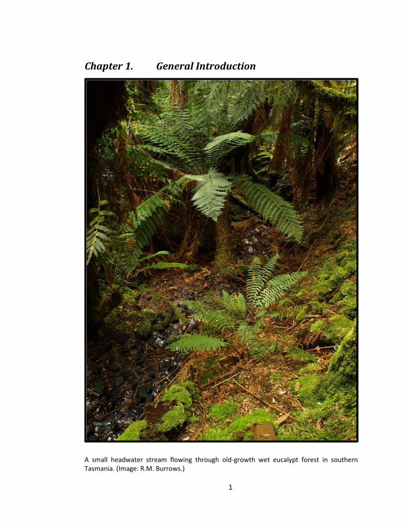
A small headwater stream flowing through old-growth wet eucalypt forest in southern Tasmania. (Image: R.M. Burrows.)

2

Freshwater ecosystems and anthropogenic disturbance

Freshwater ecosystems cover approximately 0.8% of the planet’s surface,

containing less than 0.01% of the world’s freshwater (Wetzel, 1975; Dudgeon et al.,

2006). Of these freshwater systems, humans arguably rely most heavily on streams

and rivers. Consequently, they have become some of the most altered and

threatened ecosystems in the world; dam construction, irrigation, riparian clearing,

and waste disposal all directly affect streams and rivers (Malmqvist and Rundle,

2002). However, our impact extends beyond direct interactions with them because

the water contained within streams and rivers is ultimately derived from the

surrounding catchment. Freshwater ecosystems are therefore inextricably linked

with their catchments. This is particularly true for headwater streams which are

highly integrated with the surrounding terrestrial environment (Wipfli et al., 2007).

This thesis focuses on the impact of clearfell, burn, and sow (CBS) forestry on

some key structural (woody debris and dissolved organic matter composition) and

functional (OM decomposition and nutrient uptake) characteristics of forested,

headwater streams flowing through wet eucalypt forest in southern Tasmania.

Ensuring that forest harvesting does not adversely affect headwater streams and

downstream ecosystems is important because human use of headwater streams

and their surrounding catchment is only expected to increase as our population

expands. In light of this expanding population, not only will it become increasingly

difficult to preserve their biota and ecological processes, it will become difficult to

secure them for human use (Downes et al., 2002). It is therefore important that

anthropogenic disturbance to headwaters is monitored and assessed so that we can

develop sustainable management strategies that minimise any negative effects and

maintain their ecological integrity.

3

1.1. Assessing disturbance in streams and rivers

A disturbance, whether natural or anthropogenic, is just one event

constituting a perturbation upon an ecosystem. The second event following a

perturbation is the response of an ecosystem (Glasby and Underwood, 1996). The

response of an ecosystem to disturbance can be described in terms of resistance or

resilience stability. Resistance is a measure of an ecosystem’s ability to resist or

remain unchanged after disturbance and resilience describes an ecosystem’s ability

to recover or return to its pre-disturbance state (Holling, 1973; Lake and Barmuta,

1986; Power, 1999). Measuring the response of streams and rivers to anthropogenic

disturbance is critical if they are to be managed to best maintain their ecological

integrity and reduce adverse whole-catchment impacts (Downes et al., 2002; Wipfli

et al., 2007). Ecological integrity has many definitions but has recently been defined

as:

‘the degree to which the physical, chemical and biological components

(including composition, structure and process) of an ecosystem and their

relationships are present, functioning and maintained close to a reference condition

reflecting negligible or minimal anthropogenic impacts’ (Schallenberg et al., 2011).

However, an important question that arises is what variables of running

waters should be measured to best capture any response that occurs after

anthropogenic disturbance and assess ecological integrity? The measurable

variables within an ecosystem can ultimately be categorised as either structural or

functional. Structural variables refers to spatiotemporal patterns describing the

physical (channel morphology and organic matter), chemical (nutrient

concentrations), and/or biological (species diversity and abundance) components of

an ecosystem (Fisher et al., 2007; Sandin and Solimini, 2009). Functional attributes

have many definitions but can generally be defined as the rates and processes

within an ecosystem (Meyer, 1997; Jax, 2005). Accurately assessing the response of

a freshwater ecosystem to anthropogenic disturbance requires measurement of

4

both structural and functional variables (Gessner and Chauvet, 2002; Young et al.,

2008). This is because disturbance can cause changes to structural but not

functional variables (Death et al., 2009), to functional but not structural variables

(McKie and Malmqvist, 2009), or to both (Kreutzweiser et al., 2008). Without

measuring both the structural and functional response of an ecosystem to

anthropogenic disturbance it is difficult to make informed assessments regarding

changes in ecological integrity. It is also important to recognise that natural

ecosystems are dynamic and their structural and functional components vary in

response to environmental conditions and natural disturbance (e.g. climate,

wildfire, and species lifecycles). In some instances, changes due to natural

disturbance (i.e. wildfire) can be greater than occurs after anthropogenic

disturbance (i.e. forest harvesting) (Chen et al., 2005). Therefore, when assessing

and discussing the impact of natural disturbance it is necessary to view the

structural and functional response of an ecosystem in context of any natural

variability (Downes et al., 2002; Schallenberg et al., 2011).

1.2. Headwater streams

Forested headwater streams are an important ecological component of the

landscape. They are very abundant, contributing up to 80% of the channel length of

a river system (Bryant et al., 2007; Richardson and Danehy, 2007), and provide a

variety of ecosystem services to downstream aquatic and near-shore terrestrial

habitats including water, nutrients, invertebrates, and organic matter (Richardson

and Danehy, 2007; Wipfli et al., 2007). Despite their importance to catchment-scale

ecological processes, they are perhaps the most poorly understood and neglected

component of a river system (Richardson and Danehy, 2007). Their obscurity results

from two main reasons. First, these small channels are often hidden from view

beneath the forest canopy in steep terrain, and are thus largely unmapped (Bryant

et al., 2007; Richardson and Danehy, 2007) and difficult to study. Second, there is no

universal definition of headwater streams in the literature (Benda et al., 2004).

5

A universal definition of headwater streams, like many other aquatic

ecosystems, is difficult because their geomorphic (discharge and catchment area)

and biological (species diversity and abundance) components depend on local and

regional environmental factors, such as climate, geology and topography

(Richardson and Danehy, 2007). As such, definitions vary geographically. For

instance, in Tasmania headwater streams are defined as wetted channels with a

catchment of less than 50 ha (Forest Practices Board, 2000), whereas in the Pacific

Northwest headwater streams are classified as catchments less than 100 ha with a

bankfull width of <3 m (Richardson and Danehy, 2007). A more general way to

define headwater streams is using a channel-ordering system such as the Strahler

system (Gordon et al., 2004). In the Strahler system a first order stream is the

smallest collection channel of water (Figure 1.1). This system may be overly simple,

but it provides a good conceptual framework when describing the size of streams.

Figure 1.1. A schematic representation of an upland catchment showing the drainage divide (dashed black

line) with stream channels labelled using the Strahler channel ordering system.

According to the River Continuum Concept, forested headwater streams are

closely connected to riparian vegetation and upland terrestrial systems because of

their low ratio of surface area to channel length (Vannote et al., 1980; Richardson

and Danehy, 2007). This close connection with the surrounding terrestrial landscape

6

means that they are subject to large inputs of allochthonous (i.e. originating outside

the stream) OM and nutrients relative to stream size (Wipfli et al., 2007). A closed

canopy in most forested headwater streams leads to primary production being low

(Kiffney et al., 2004), and they are generally dominated by heterotrophic activity

(Clapcott and Barmuta, 2009). Consequently, their structure and function are

strongly influenced by the supply of allochthonous OM and nutrients (Vannote et

al., 1980). Figure 1.2 shows some of the major structural and functional components

of forested, headwater streams that are influenced by their close connection with

the surrounding terrestrial environment.

Riparian vegetation is a major source of stream OM input to headwater

streams, contributing leaf litter (often termed CPOM: coarse particulate organic

matter), fine and large woody debris (FWD and LWD respectively), and invertebrates

(Figure 1.2) (Richardson and Danehy, 2007). As much as 99% of OM entering

headwater streams can be attributed to riparian vegetation (Fisher and Likens,

1973). Leaf litter input is particularly important as an energy source in these

heterotrophic systems. Fungi and bacteria breakdown leaf litter and make it more

palatable for aquatic invertebrates (Gulis and Suberkropp, 2003). These aquatic

invertebrates, along with those originating from the terrestrial ecosystem, become

an energy source for other invertebrates and vertebrates either in the same stream

reach or in downstream ecosystems (Figure 1.2) (Ormerod et al., 2004; Romaniszyn

et al., 2007).

Woody debris is a major source of OM derived from riparian vegetation

(Reeves et al., 2003; Hassan et al., 2005), and is essential for providing structural

complexity in stream channels (Montgomery et al., 1995), contributing to sediment

storage (Smock et al., 1989; Gomi et al., 2001), and maintaining biodiversity through

the creation and maintenance of habitat (Wilkins and Peterson, 2000; Jones and

Daniels, 2008; Rinella et al., 2009). Although woody debris itself is not a labile

energy source to stream biota, the attached algal and bacterial biofilms and the

7

processing of leaf litter and sediment stored behind woody debris increase biotic

processing and nutrient retention (Figure 1.2) (Valett et al., 2002; Bernhardt et al.,

2003; Bond et al., 2006; Roberts et al., 2007).

Dissolved organic matter (DOM) can also contribute a substantial proportion

of the total OM entering a forested headwater stream, constituting greater than

80% of the total mass of OM export (Wallace et al., 1995; Kiffney et al., 2000;

Karlsson et al., 2005). DOM consists of a complex mixture of carbon (DOC), nitrogen

(DON), and phosphorus (DOP). DOM is essential to headwater stream ecosystems

because the assimilation of DOM by stream heterotrophic life is one of the principle

ways that carbon (C) is incorporated into the aquatic food web (Findlay and

Sinsabaugh, 1999). In forested streams, a large proportion of DOM is derived from

the leaching of terrestrial plant and soil OM, and the biotic processing of terrestrial

particulate inputs (Findlay and Sinsabaugh, 1999; McKnight et al., 2001).

Coupled with the input and processing of OM is the input and processing of

nutrients. The fate of input nutrients is important because large fluxes of nutrients,

such as nitrogen (N) and phosphorus (P), to downstream freshwater and marine

ecosystems can lead to adverse environmental impacts, such as eutrophication and

acidification (Alexander et al., 2007), and even the deterioration of water quality for

human consumption (Dodds and Oakes, 2008). However, the low ratio of surface

area to channel length in headwater streams means that there is large opportunity

for headwater streams to processes nutrients and mediate their export (Peterson et

al., 2001). The uptake and processing of nutrients, as well as DOM, in headwater

streams are controlled by a combination of biotic and abiotic processes that occur

predominately on the stream bottom or benthos (Webster and Valett, 2006). The

abiotic processes are linked mostly to the sediment characteristics of a stream and

include adsorption, desorption, precipitation, and dissolution (Webster and Valett,

2006). The biotic processes controlling uptake and processing include autotrophic

8

(i.e. benthic algae) and heterotrophic (i.e. sediment bacteria and microbial biofilms)

uptake (Webster and Valett, 2006).

Figure 1.2. Schematic showing the close connection that forested, headwater streams have with their

surrounding terrestrial environment. The figure highlights the dominant input sources of organic matter (OM)

and nutrients, their processing, and export. Woody debris and coarse particulate organic matter (CPOM) are

input into the stream directly from riparian vegetation or transported with water flow from upstream. Algal

and bacterial biofilms, as well as fungi then grow on their surfaces. Sediment and CPOM are trapped behind

woody debris where they become processed by bacteria, algae, and aquatic invertebrates. Terrestrial

invertebrates fall into the stream and become an energy source for other biotia. Aquatic invertebrates can

also emerge from the stream, becoming energy sources for terrestrial biotia. DOM and nutrients are leached

9

from terrestrial OM and soils or input via groundwater recharge. The uptake and cycling of OM and nutrients

occurs while they are being continuously transported downstream. This illustration has been adapted from

Richard and Danehy (2007).

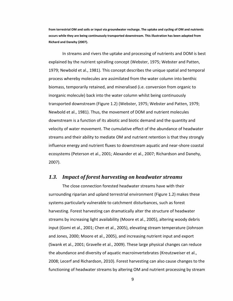
In streams and rivers the uptake and processing of nutrients and DOM is best

explained by the nutrient spiralling concept (Webster, 1975; Webster and Patten,

1979; Newbold et al., 1981). This concept describes the unique spatial and temporal

process whereby molecules are assimilated from the water column into benthic

biomass, temporarily retained, and mineralised (i.e. conversion from organic to

inorganic molecule) back into the water column whilst being continuously

transported downstream (Figure 1.2) (Webster, 1975; Webster and Patten, 1979;

Newbold et al., 1981). Thus, the movement of DOM and nutrient molecules

downstream is a function of its abiotic and biotic demand and the quantity and

velocity of water movement. The cumulative effect of the abundance of headwater

streams and their ability to mediate OM and nutrient retention is that they strongly

influence energy and nutrient fluxes to downstream aquatic and near-shore coastal

ecosystems (Peterson et al., 2001; Alexander et al., 2007; Richardson and Danehy,

2007).

1.3. Impact of forest harvesting on headwater streams

The close connection forested headwater streams have with their

surrounding riparian and upland terrestrial environment (Figure 1.2) makes these

systems particularly vulnerable to catchment disturbances, such as forest

harvesting. Forest harvesting can dramatically alter the structure of headwater

streams by increasing light availability (Moore et al., 2005), altering woody debris

input (Gomi et al., 2001; Chen et al., 2005), elevating stream temperature (Johnson

and Jones, 2000; Moore et al., 2005), and increasing nutrient input and export

(Swank et al., 2001; Gravelle et al., 2009). These large physical changes can reduce

the abundance and diversity of aquatic macroinvertebrates (Kreutzweiser et al.,

2008; Lecerf and Richardson, 2010). Forest harvesting can also cause changes to the

functioning of headwater streams by altering OM and nutrient processing by stream

10

biota (Sabater et al., 2000; McKie and Malmqvist, 2009; Clapcott and Barmuta,

2010; Kreutzweiser et al., 2010). Given that headwaters strongly influence energy

and nutrient fluxes to downstream aquatic and near-shore coastal ecosystems,

changes to the structure and function of headwater streams caused by forest

harvesting may have profound implications not only for the ecological integrity of

headwater streams, but the whole catchment.

1.4. Tasmanian headwater streams and clearfell, burn and sow

(CBS) forestry

In southern Tasmania headwater streams flowing through wet eucalypt

forests are numerous, contributing over 50% of the channel length of river systems

(Clapcott, 2007; Gooderham et al., 2007). They lack a defined riparian zone, are

characterised by an evergreen closed canopy, with the major form of energy from

riparian organic matter inputs (Clapcott, 2007; Clapcott and Barmuta, 2009). Mean

daily flow is low (≈ 1 to 3 L s-1) but they are commonly ‘flashy’ and perennial

(Clapcott, 2007; Clapcott and Barmuta, 2009). These small headwater streams have

a high morphological diversity and their structure and function can be highly

heterogeneous, relying strongly on local environmental characteristics such as the

presence of exposed rocks or tree roots (Gooderham et al., 2007; Clapcott and

Barmuta, 2009). The great physical complexity that characterises Tasmanian

headwater streams places them within the upstream heterogeneous zone (UHZ); as

proposed by Gooderham et al. (2007).

Vegetation disturbance due to CBS forestry is a major stressor on headwater

streams flowing through southern Tasmanian wet eucalypt forests. CBS is the

standard silvicultural operation for lowland wet eucalypt forests on hillsides with

slopes less than 20° (Hickey and Wilkinson, 1999; Forest Practices Board, 2000). As

the name suggests, CBS forestry involves clearfelling areas of forest (called coupes),

burning the harvested coupe to provide a receptive mineral seedbed, and aerial

sowing to supplement eucalypt regeneration (Hickey and Wilkinson, 1999). Eucalypt

11

coupes are usually re-harvested after 80 to 100 years of regeneration (Hickey et al.,

2001).

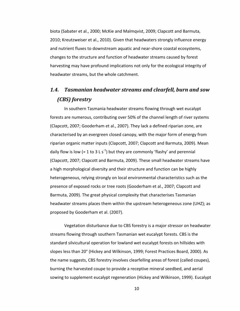
When CBS forestry occurs in the upper catchment, headwater streams often

originate or flow through sections of CBS-affected coupes (Figure 1.3). The

CBS-affected study streams in this thesis either originate in, or are affected by, only

one harvesting operation. The Tasmanian Forest Practices Code (2000) currently

provides for the protection of headwater streams at the landscape- and reach-scale.

At the landscape-scale, CBS coupes are dispersed across the landscape and through

time (termed ‘coupe dispersal’). At the reach-scale, government legislation

stipulates a 10 m machinery exclusion zones (MEZ) around first- and second-order

headwater streams, but still with harvesting of riparian vegetation where practical

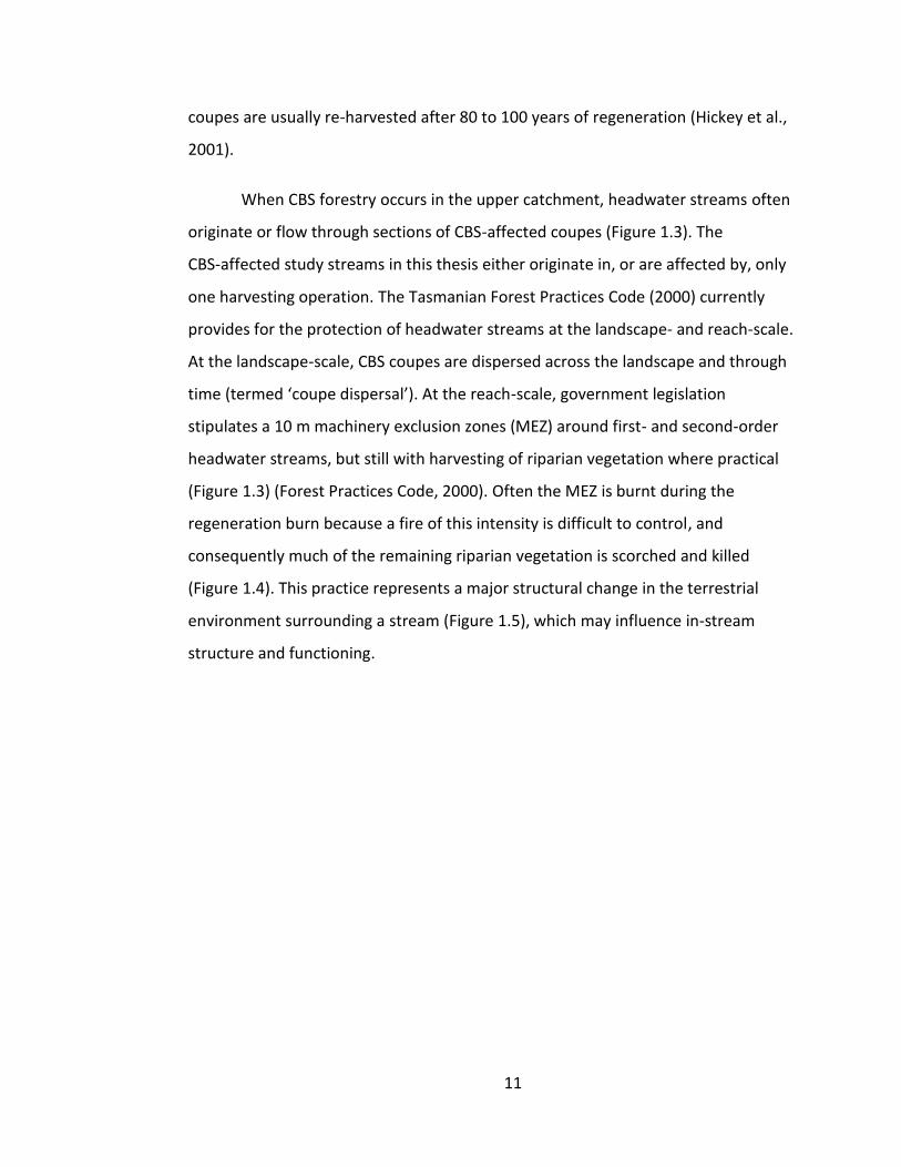
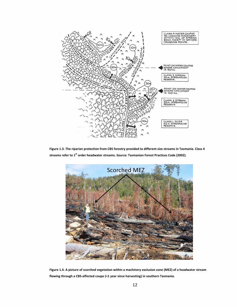
(Figure 1.3) (Forest Practices Code, 2000). Often the MEZ is burnt during the

regeneration burn because a fire of this intensity is difficult to control, and

consequently much of the remaining riparian vegetation is scorched and killed

(Figure 1.4). This practice represents a major structural change in the terrestrial

environment surrounding a stream (Figure 1.5), which may influence in-stream

structure and functioning.

12

Figure 1.3. The riparian protection from CBS forestry provided to different size streams in Tasmania. Class 4

streams refer to 1st

order headwater streams. Source: Tasmanian Forest Practices Code (2002).

Figure 1.4. A picture of scorched vegetation within a machinery exclusion zone (MEZ) of a headwater stream

flowing through a CBS-affected coupe (<1 year since harvesting) in southern Tasmania.

13

Figure 1.5. Photograph of a stream in (a) old-growth (OG) and (b) CBS-affected forest.

The importance of headwater streams in the landscape has led to concern by

both foresters and the general public about the impacts of CBS forestry, which was

raised during a review of the Soil and Water provisions of the Tasmanian Forest

Practices Code (Forest Practices Board, 2000). A better understanding of how CBS

forestry affects the structure and functioning of headwater streams was needed,

with the aim of enhancing the potential to reduce whole-catchment adverse

impacts. Consequently, research was initiated that assessed the impact of CBS

forestry on forested headwater streams, and more specifically its effects on stream

metabolism at different scales of measurement (Clapcott, 2007). This research

identified that the metabolic signature of headwater streams flowing through wet

eucalypt forest was highly heterogeneous in space and time, being shaped by

stream temperature, hydrology, and the physical and chemical properties of benthic

sediment (Clapcott, 2007). Furthermore, the research found that 2 to 5 years after

harvesting, autotrophic activity was stimulated, and led to increased metabolic

rates.

14

Only autotrophic processes displayed a recovery, with key measures of

heterotrophic activity showing an increase in variability over time (2–15 y),

suggesting a short-term lack of resistance and resilience of heterotrophic activity to

CBS forestry (Clapcott, 2007). However, because headwater streams are structurally

and functionally heterogeneous in space and time and forest practices

simultaneously alter many environmental variables, it can be difficult to isolate

individual effects (Walters et al., 1988). Therefore, a key recommendation of this

research was further investigation using a multiple before-after control-impact

(MBACI) study. In 2007 this was initiated with special emphasis on measures of

organic matter (OM) decomposition of benthic sediment. This MBACI study

represents one of the first replicated studies contrasting OM decomposition before

and after clearfell forestry carried out under industry best practice. Chapter 5 of my

thesis summarises the findings of this research.

Although part of my thesis deals with the impact of CBS forestry on OM

decomposition in headwater streams, there is a lack of information regarding other

important structural and functional characteristics. As such, the remaining chapters

of my thesis will focus on the impact that CBS forestry has on several key structural

(woody debris and dissolved organic matter composition) and functional (nutrient

uptake) characteristics.

1.5. Contributing to the understanding of how disturbance

influences the structure and function of headwater streams

This thesis contributes to the theoretical framework regarding how major

reach-scale anthropogenic disturbances influence the structure (physical and

chemical) and function of forested, headwater streams. It will also contribute to the

understanding of the resistance and resilience of some structural and functional

measures to anthropogenic disturbance. Small headwater streams flowing through

15

the wet eucalypt forest in southern Tasmania are an ideal ecosystem to study the

impact of forest harvesting on structural and functional variables, because these

streams are not influenced by transient effects associated with landscape

anthropogenic disturbances other than forest harvesting, such as urban

development and agriculture.

1.6. Thesis aims

Ensuring that forest harvest practices do not adversely affect headwater

streams is fundamental if we want to develop sustainable management strategies

that minimise the loss of ecological integrity and whole catchment impacts. My

overall aim is to measure several key structural (woody debris and dissolved organic

matter composition) and functional (OM processing and nutrient uptake)

characteristics of small headwater streams flowing through wet eucalypt forest in

southern Tasmania and to investigate the influence that CBS forest harvesting has

upon these characteristics. To achieve this aim, my thesis forms four research

chapters focusing on woody debris input and function, stream dissolved organic

matter, benthic OM decomposition, and reach-scale nutrient uptake. The

integration of these complimentary areas of research should enable a more

comprehensive understanding of the impact of CBS forestry on the ecology of

headwater streams. This thesis will primarily focus on the short-term (<19 years

after harvesting) impact of CBS forestry on headwater streams because the current

CBS prescriptions for headwater streams only became operational in 1993. The

precise timeframe will depend on the experiment design described in each

individual chapter. The potential longer-term (>19 years after harvest) impacts and

implications will be discussed throughout.

Chapters 2 to 5 of this thesis are written as individual research manuscripts,

which have either been submitted or are intended for submission for publication.

These are presented as four distinct chapters as follows:

16

Chapter 2. Woody debris input and function in old-growth and clearfell forestry

modified headwater streams

Woody debris is a fundamental structural characteristic of headwater streams.

My aim in Chapter 2 was to quantitatively assess the short-term (<7 years)

difference in the quantity (abundance and volume) and functional role of woody

debris pieces between CBS-affected and old-growth (OG) headwater streams in

southern Tasmania. To do this I surveyed five OG and five CBS-affected headwater

streams flowing through wet eucalypt forest in southern Tasmania.

Chapter 3. Greater phosphorus uptake in forested headwater streams modified by

clearfell forestry

Nutrient uptake is an important functional process in headwater streams

which as implications for the whole catchment. Chapter 3 determines if in-stream

nutrient uptake varies between individual reaches flowing through OG and

CBS-affected streams. This chapter builds on Chapter 2 by investigating whether

woody debris characteristics, along with other environmental variables, influences

rates of nutrient uptake. To do this, I measured key stream environmental variables

(e.g. light, and wood debris) and used short-term nutrient addition experiments to

measure the uptake length, uptake velocity and uptake rate of ammonium (NH4)

and phosphate (as soluble reactive phosphorus; SRP) in three OG and four

CBS-affected headwater stream reaches.

Chapter 4. Allochthonous dissolved organic matter controls bacterial carbon

production in forested, headwater streams

Chapter 4 used fluorescent characterisation of DOM to investigate how DOM

source and composition, along with various reach environmental variables,

influence rates of benthic BCP in twenty headwater streams in southern Tasmania.

Furthermore, this chapter also assesses whether CBS forest harvesting of headwater

stream reaches influence DOM source and composition.

17

Chapter 5. Effect of clearfell harvesting on organic matter decomposition differs

among benthic habitats in forested, headwater streams

Chapter 5 assesses the impact that CBS forestry has upon rates of OM

decomposition in benthic sediment of headwater streams. This chapter summarises

part of the MBACI study initiated in 2007 by focusing on two complimentary

measures of OM decomposition; bacterial carbon production (BCP) was used to

measure the productivity of bacterial populations and cotton strip assays were used

to assess cellulose decomposition by microbial (aquatic hyphomycetes, bacteria,

and algae) processes. As such, this chapter assesses how a key stream function, OM

decomposition, is altered by the structural change caused by forest harvesting.

Chapter 6. General discussion

Chapter 6 provides a synthesis of the key findings from Chapters 2 to 5 and

highlights the important ecological concepts that have implications for the

management of headwater streams that are affected by CBS forestry.

This chapter has been removed for

copyright or proprietary reasons.

CHAPTER 2

Woody debris input and function in old-growth and clearfelled headwater streams

Published in:

http://www.sciencedirect.com/science/article/pii/S0378112712005221

Burrows, R. M., Magierowski, R. H., Fellman, J. B., and Barmuta, L. A. 2012. Woody debris input and function in old-growth and clear-felled

headwater streams. Forest Ecology and Management, 286: 73-80.

http://www.sciencedirect.com/science/article/pii/S0378112712005221

CHAPTER 3

Greater phosphorus uptake in forested headwater streams modified by clearfell forestry

Published in:

http://link.springer.com/article/10.1007%2Fs10750-012-1332-5

Burrows, R. M., Fellman, J. B., Magierowski, R. H., and Barmuta, L. A. 2012. Greater phosphorus uptake in forested headwater streams

modified by clearfell forestry. Hydrobiologia, 703: 1-14.

http://link.springer.com/article/10.1007%2Fs10750-012-1332-5

CHAPTER 4

Allochthonous dissolved organic matter controls bacterial carbon production in old-growth and clearfelled headwater streams

Published In:

http://www.bioone.org/doi/abs/10.1899/12-163.1

Burrows, R. M., Fellman, J. B., Magierowski, R. H., and Barmuta, L. A. 2013. Allochthonous dissolved organic matter controls bacterial

carbon production in old-growth and clearfelled headwater streams. Freshwater Science, 32(3), DOI: 10.1899/12-163.

http://www.bioone.org/doi/abs/10.1899/12-163.1

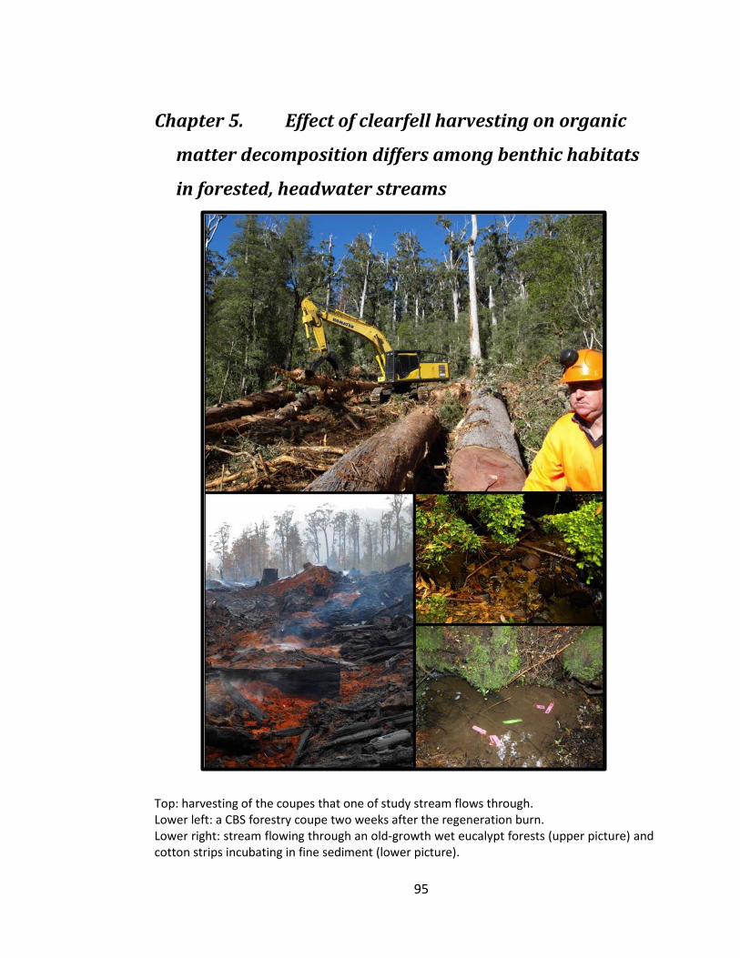
95

Chapter 5. Effect of clearfell harvesting on organic

matter decomposition differs among benthic habitats

in forested, headwater streams

Top: harvesting of the coupes that one of study stream flows through. Lower left: a CBS forestry coupe two weeks after the regeneration burn. Lower right: stream flowing through an old-growth wet eucalypt forests (upper picture) and cotton strips incubating in fine sediment (lower picture).

96

5.1. Abstract

Organic matter (OM) decomposition of coarse gravel and fine benthic

sediment, along with water temperature, were assessed in four clearfell harvested

and two undisturbed headwater streams flowing through Tasmanian wet eucalypt

forest. Bacterial carbon production and cellulose decomposition (together referred

to as OM decomposition throughout) were recorded seasonally 3–5 years before

and 2–4 years after harvesting. A staircase design (staggered harvesting treatments)

was employed to distinguish transient (natural variability) from harvesting effects.

Clearfell harvesting altered the stream temperature regime, raising the yearly mean

between 0.25 and 0.94°C, and raising the maximum between 0.84 and 1.6°C. The

response in OM decomposition to clearfell harvesting differed between years and

among benthic habitats. In coarse gravel habitat, there was a significant decrease in

rates of cellulose decomposition in the 2nd and 4th year after harvesting, and a

significant decrease in bacterial carbon production in the 3rd year after harvesting.

However, I found a significant increase in rates of bacterial carbon production of

fine sediment habitat in the 2nd and 4th year after harvesting. The contrasting

response of OM decomposition between habitats suggests that habitat-specific

changes are occurring after clearfell harvesting, such as physical substrate

disturbance in coarse gravel but not fine sediment. My findings highlight the need

for staircase study designs when assessing the impact of disturbance on ecological

variables which are likely to show high spatial and temporal heterogeneity in their

response. Without accounting for this variability it may be difficult to detect any

response to a disturbance.

5.2. Introduction

The availability and decomposition of organic matter (OM) in freshwater

streams is largely driven by ecosystem processes associated with the activity of

benthic heterotrophic aquatic fungi, bacteria, and algae (Gulis and Suberkropp,

2003). For instance, the assimilation of dissolved organic carbon (DOC) by aquatic

97

heterotrophs represents one of the principal ways that OM is incorporated into the

aquatic food web (Findlay and Sinsabaugh, 1999). The decomposition of terrestrially

derived OM is particularly important in forested, headwater streams where it is the

dominant source of energy for aquatic food webs (Young et al., 2008) and strongly

influences particulate and dissolved OM fluxes to downstream aquatic and near-

shore coastal ecosystems (Peterson et al., 2001). Measurements of OM

decomposition in headwater streams can thus provide important information about

the functional integrity of the entire fluvial network (Tiegs et al., 2007; Young et al.,

2008).

Natural variation in the stream environment can alter OM decomposition.

For example, OM decomposition can be influenced by surface water and sediment

nutrient concentration (Gulis and Suberkropp, 2003; Clapcott and Barmuta, 2009;

Gravelle et al., 2009), temperature (White et al., 1991; Menéndez et al., 2003;

Clapcott and Barmuta, 2009), light availability (Lagrue et al., 2011), and autotrophic

activity (Rees et al., 2005; Guillemette and del Giorgio, 2011). Seasonal variability in

many of these variables can lead to different patterns of OM decomposition

throughout the year. For example, during the winter months lower temperatures

(Clapcott and Barmuta, 2009) and greater streams flows (Laćan et al., 2010) can

reduce OM decomposition. However, anthropogenic disturbance can also alter

stream environmental variables, such as benthic organic matter and discharge,

which, in turn, can affect OM processing (Tuchman and King, 1993; Wipfli et al.,

2007; Woodcock and Huryn, 2007).

Forest clearfell harvesting is one such anthropogenic disturbance that can

cause large changes to the stream environment (Swank et al., 2001; Gravelle et al.,

2009) with implications for OM decomposition (McKie and Malmqvist, 2009;

Clapcott and Barmuta, 2010; Lecerf and Richardson, 2010). It is critical that land

managers understand the influence of forest harvesting on OM decomposition so

that deleterious effects downstream, such as an altered energy supply, can be

98

mitigated. However, research on the impact of clearfell harvesting on OM

decomposition in streams is conflicting. Previous research has found increased OM

decomposition after harvesting (McKie and Malmqvist, 2009), while others found a

decrease (Kreutzweiser et al., 2008; Lecerf and Richardson, 2010), or no difference

(Kreutzweiser et al., 2010). These conflicting findings may be because small streams

are structurally and functionally heterogeneous in space and time (Vannote et al.,

1980; Gooderham et al., 2007). Without accounting for this variability it is difficult to

isolate effects caused by forest harvesting from natural variability (Walters et al.,

1988; Downes et al., 2002).

Multiple before-after control-impact (MBACI) experiments are commonly

recommended for the assessment of perturbations in streams because they account

for spatial and temporal variability between streams (Downes et al., 2002).

However, standard MBACI designs have been criticised because they do not

distinguish between deliberate treatment effects and transient effects due to

natural changes (i.e. a time-treatment interaction) (Walters et al., 1988). For

instance, the response of OM decomposition to forest harvesting may have

previously been influenced by post-logging drought (Benfield et al., 2001;

Kreutzweiser et al., 2010). To control for this time-treatment interaction, Walters et

al. (1998) recommended that disturbances to treated locations be staggered over

time, and termed these ‘staircase designs’.

Clearfell, burn and sow (CBS) forestry represents a major disturbance to

headwater streams flowing through the wet eucalypt forests of southern Tasmania

(Figure 1.5). CBS is a form of forest harvesting that involves the felling of all trees

from a specific area, the burning of this area to provide a receptive mineral

seedbed, and the sowing of seed to ensure eucalypt regrowth (Hickey and

Wilkinson, 1999; Forest Practices Board, 2000). There are no formal buffer strips,

but a 10 m machinery exclusion zone (MEZ) is required around small headwater

streams (Forest Practices Board, 2000). Despite this, the vegetation in the MEZ is

99

often scorched and killed during the regeneration burn (Clapcott and Barmuta,

2010). Previous space-for-time surveys in these headwater streams identified that

CBS forestry causes a short-term (<5 years) increase in bacterial and microbial OM

decomposition, and that this was strongly associated with increased sediment

temperature (Clapcott, 2007; Clapcott and Barmuta, 2010). This study builds on this

previous research but uses an MBACI approach that includes staggered treatments

in time (i.e. staircase analysis).

Two complementary measures of OM processing were used: bacterial

carbon production (BCP) assessed the activity of benthic bacterial populations

(Buesing and Gessner, 2003b), and cellulose decomposition potential measured the

activity of benthic microbial populations (aquatic fungi, bacteria, and algae)

(Boulton and Quinn, 2000). Based on previous research I expected that CBS forestry

would increase the short-term (<4 years) rates of BCP and microbial cellulose

decomposition, driven largely by elevated sediment temperature. This study

represents the first replicated study with staggered treatments contrasting organic

matter-related measures of ecosystem processes before and after clearfell forestry

carried out under industry best practice.

5.3. Methods

5.3.1. Study region and streams

The study was conducted in the Warra Long Term Ecological Research (LTER)

Site (Neyland et al., 2000), which is situated within the Tasmanian Southern Ranges

(TSR) bioregion, as described by the Interim Biogeographic Regionalisation for

Australia (IBRA) (Thackway and Cresswell, 1995). The study region has a rugged

topography and a temperate climate with a mean annual minimum and maximum

temperatures of 5.4 and 13.7°C, respectively. Mean annual rainfall exceeded

1600mm during the study period (Table 5.1) (Bureau of Meteorology, 2012). The

geology of the region is dominated by Permo-Triassic sediments and Jurassic basic

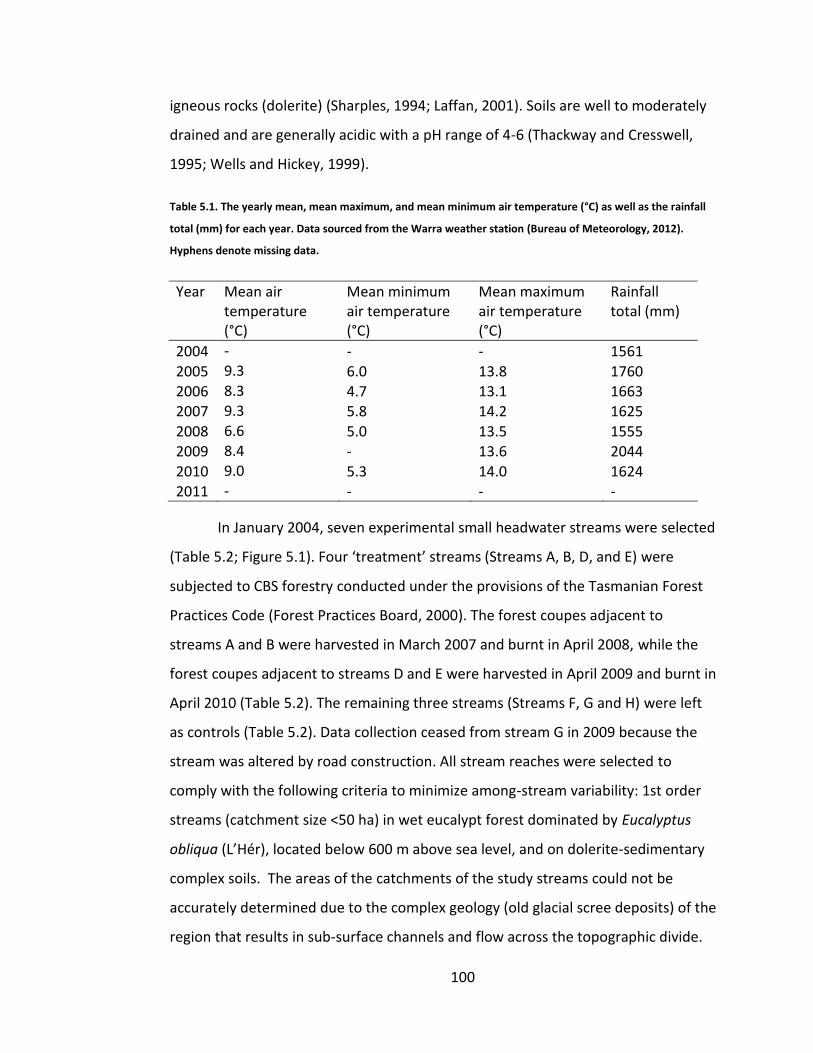
100

igneous rocks (dolerite) (Sharples, 1994; Laffan, 2001). Soils are well to moderately

drained and are generally acidic with a pH range of 4-6 (Thackway and Cresswell,

1995; Wells and Hickey, 1999).

Table 5.1. The yearly mean, mean maximum, and mean minimum air temperature (°C) as well as the rainfall

total (mm) for each year. Data sourced from the Warra weather station (Bureau of Meteorology, 2012).

Hyphens denote missing data.

Year Mean air temperature (°C)

Mean minimum air temperature (°C)

Mean maximum air temperature (°C)

Rainfall total (mm)

2004 - - - 1561

2005 9.3 6.0 13.8 1760 2006 8.3 4.7 13.1 1663 2007 9.3 5.8 14.2 1625

2008 6.6 5.0 13.5 1555 2009 8.4 - 13.6 2044

2010 9.0 5.3 14.0 1624 2011 - - - -

In January 2004, seven experimental small headwater streams were selected

(Table 5.2; Figure 5.1). Four ‘treatment’ streams (Streams A, B, D, and E) were

subjected to CBS forestry conducted under the provisions of the Tasmanian Forest

Practices Code (Forest Practices Board, 2000). The forest coupes adjacent to

streams A and B were harvested in March 2007 and burnt in April 2008, while the

forest coupes adjacent to streams D and E were harvested in April 2009 and burnt in

April 2010 (Table 5.2). The remaining three streams (Streams F, G and H) were left

as controls (Table 5.2). Data collection ceased from stream G in 2009 because the

stream was altered by road construction. All stream reaches were selected to

comply with the following criteria to minimize among-stream variability: 1st order

streams (catchment size <50 ha) in wet eucalypt forest dominated by Eucalyptus

obliqua (L’Hér), located below 600 m above sea level, and on dolerite-sedimentary

complex soils. The areas of the catchments of the study streams could not be

accurately determined due to the complex geology (old glacial scree deposits) of the

region that results in sub-surface channels and flow across the topographic divide.

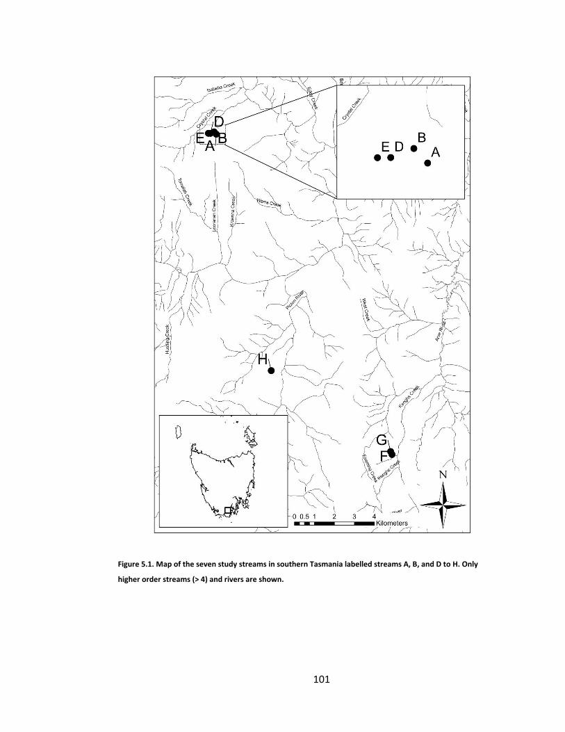
101

Figure 5.1. Map of the seven study streams in southern Tasmania labelled streams A, B, and D to H. Only

higher order streams (> 4) and rivers are shown.

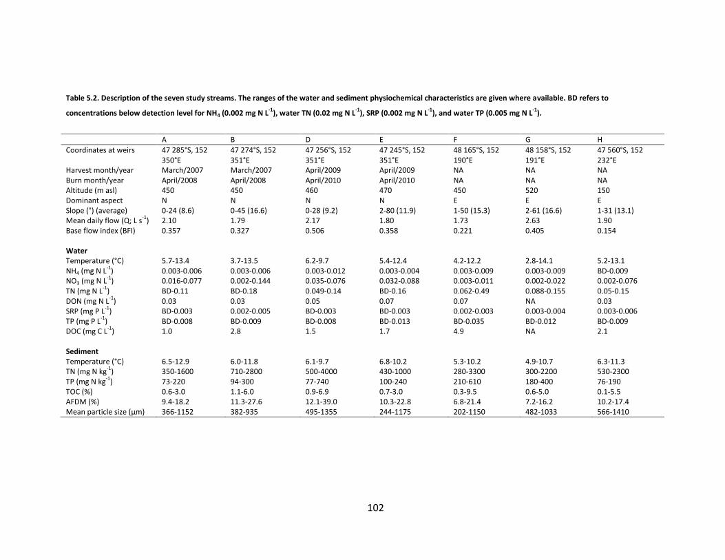
102

Table 5.2. Description of the seven study streams. The ranges of the water and sediment physiochemical characteristics are given where available. BD refers to

concentrations below detection level for NH4 (0.002 mg N L-1

), water TN (0.02 mg N L-1

), SRP (0.002 mg N L-1

), and water TP (0.005 mg N L-1

).

A B D E F G H

Coordinates at weirs 47 285°S, 152 350°E

47 274°S, 152 351°E

47 256°S, 152 351°E

47 245°S, 152 351°E

48 165°S, 152 190°E

48 158°S, 152 191°E

47 560°S, 152 232°E

Harvest month/year March/2007 March/2007 April/2009 April/2009 NA NA NA Burn month/year April/2008 April/2008 April/2010 April/2010 NA NA NA Altitude (m asl) 450 450 460 470 450 520 150 Dominant aspect N N N N E E E Slope (°) (average) 0-24 (8.6) 0-45 (16.6) 0-28 (9.2) 2-80 (11.9) 1-50 (15.3) 2-61 (16.6) 1-31 (13.1) Mean daily flow (Q; L s

-1) 2.10 1.79 2.17 1.80 1.73 2.63 1.90

Base flow index (BFI) 0.357 0.327 0.506 0.358 0.221 0.405 0.154 Water Temperature (°C) 5.7-13.4 3.7-13.5 6.2-9.7 5.4-12.4 4.2-12.2 2.8-14.1 5.2-13.1 NH4 (mg N L

-1) 0.003-0.006 0.003-0.006 0.003-0.012 0.003-0.004 0.003-0.009 0.003-0.009 BD-0.009

NO3 (mg N L-1

) 0.016-0.077 0.002-0.144 0.035-0.076 0.032-0.088 0.003-0.011 0.002-0.022 0.002-0.076 TN (mg N L

-1) BD-0.11 BD-0.18 0.049-0.14 BD-0.16 0.062-0.49 0.088-0.155 0.05-0.15

DON (mg N L-1

) 0.03 0.03 0.05 0.07 0.07 NA 0.03 SRP (mg P L

-1) BD-0.003 0.002-0.005 BD-0.003 BD-0.003 0.002-0.003 0.003-0.004 0.003-0.006

TP (mg P L-1

) BD-0.008 BD-0.009 BD-0.008 BD-0.013 BD-0.035 BD-0.012 BD-0.009 DOC (mg C L

-1) 1.0 2.8 1.5 1.7 4.9 NA 2.1

Sediment Temperature (°C) 6.5-12.9 6.0-11.8 6.1-9.7 6.8-10.2 5.3-10.2 4.9-10.7 6.3-11.3 TN (mg N kg

-1) 350-1600 710-2800 500-4000 430-1000 280-3300 300-2200 530-2300

TP (mg N kg-1

) 73-220 94-300 77-740 100-240 210-610 180-400 76-190 TOC (%) 0.6-3.0 1.1-6.0 0.9-6.9 0.7-3.0 0.3-9.5 0.6-5.0 0.1-5.5 AFDM (%) 9.4-18.2 11.3-27.6 12.1-39.0 10.3-22.8 6.8-21.4 7.2-16.2 10.2-17.4 Mean particle size (µm) 366-1152 382-935 495-1355 244-1175 202-1150 482-1033 566-1410

103

5.3.2. Field procedures

5.3.2.1. Organic matter decomposition

Cellulose decomposition potential (CDP) and BCP of coarse gravel and fine

sediment habitat was assessed every three months (February, May, August, and

November) between 2004 and 2011 using identical procedures to those employed

previously by Clapcott and Barmuta (2009) in these streams. Coarse gravel habitat

consists of gravely sediment (<5 mm) that is generally located in high flow areas of

headwater streams, whereas fine sediment consists of well-sorted, depositional

sediment (<2 mm) in more protected areas of streams. CDP of sediment was

assessed using cotton strip assays (Boulton and Quinn, 2000). These were used

instead of leaf-packs because their breakdown (i.e. OM decomposition) is not

confounded by chemical variability in leaf age and/or species, thus providing a

standardised measure of organic matter decomposition (Boulton and Quinn, 2000;

Tiegs et al., 2007; Young et al., 2008). Unbleached cotton fabric (EMPA, Dübendorf,

Switizerland) was used for all assays, and the method was fully described by

Clapcott and Barmuta (2009). Briefly, ten cotton strips (35 × 60mm), held on plastic

rulers with rubber bands, were placed in pairs just beneath the surface of the

chosen habitat (either coarse gravel or fine depositional sediment) at the beginning

of each sample period. After 28 days the rulers and strips were collected, gently

rinsed and transported back to laboratory on ice. A set of cotton strips of varying

widths were soaked in stream water for 1 hour and the processed in the same way

as the other cotton strips for use as procedural controls (Clapcott and Barmuta,

2009).

BCP of coarse gravel and fine sediment was measured using the

incorporation of C14-leucine into bacterial protein (Buesing and Gessner, 2003a).

Field sampling was identical to that previously used by Clapcott and Barmuta (2009).

On the same day that the cotton strips were retrieved, approximately 50 g of

104

sediment was randomly collected from the top 10 mm of the benthic surface along

each reach and in each habitat, and placed in a 250 mL glass jar. The sediment was

gently homogenized using a sterile metal spoon and then 0.5 mL aliquots were

transferred into four plastic test tubes, one control and three replicates. Three

drops of buffered formalin (0.1% w/v sodium pyrophosphate) was added to the

control to inhibit microbial activity and 0.5 ml of C14-leucine was added to the

control and the three replicates. The test tubes were sealed and then placed in

stream water for incubation. After 60 mins, the test tubes were retrieved and the

incubation was stopped with 1 ml of 50% TCA (trichloroacetic acid) and 8 ml of

Milli-Q water. Test tubes were then stored on ice until transfer to the laboratory

refrigerator. The remaining sediment samples were stored on ice in the dark and

frozen upon return to the laboratory for later sub-sampling for chemical (total

nutrients and carbon) and physical (AFDM) characteristics.

5.3.2.2. Environmental variables

In each stream, 90° v-notch weirs were constructed at the downstream end

of each stream reach (Appendix 1) and continuous stage-height data recorded using

Odyssey capacitance water level probes (Dataflow Systems, New Zealand). Rating

curves for each weir were established with manual measurements of water level at

least every 3 months, and the River Analysis Package (Marsh et al., 2003) was used

to generate mean daily flow (l s-1) and base flow index (BFI). Water temperature was

recorded at 10 min intervals using iButton© temperature loggers (OnSolution,

Sydney, Australia). Fine sediment temperature was recorded using iButton©

temperature loggers, placed just beneath the sediment surface, at 10 min intervals

during the cotton strip incubations. Stream water was collected intermittently (1 to

4 times per year) for analysis of ambient concentrations of ammonium (NH4), nitrate

(NO3), total nitrogen (TN), total dissolved nitrogen (TDN), soluble reactive

phosphorus (SRP), and total phosphorus (TP). Samples were transferred into pre-

cleaned 50mL Sarstedt® PP reagent tubes, stored on ice and refrigerated upon

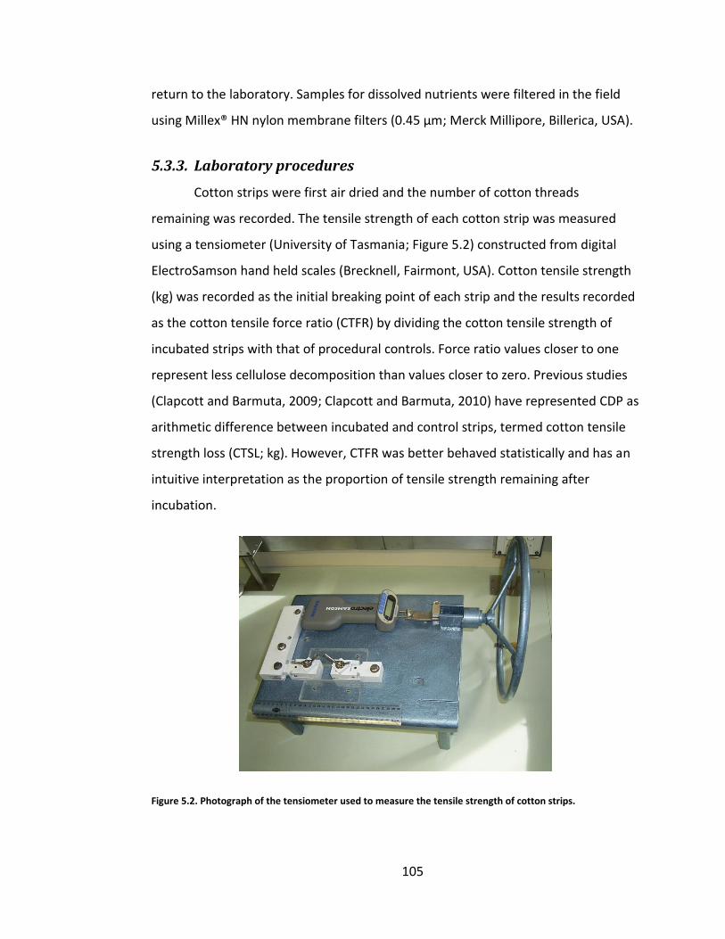
105

return to the laboratory. Samples for dissolved nutrients were filtered in the field

using Millex® HN nylon membrane filters (0.45 µm; Merck Millipore, Billerica, USA).

5.3.3. Laboratory procedures

Cotton strips were first air dried and the number of cotton threads

remaining was recorded. The tensile strength of each cotton strip was measured

using a tensiometer (University of Tasmania; Figure 5.2) constructed from digital

ElectroSamson hand held scales (Brecknell, Fairmont, USA). Cotton tensile strength

(kg) was recorded as the initial breaking point of each strip and the results recorded

as the cotton tensile force ratio (CTFR) by dividing the cotton tensile strength of

incubated strips with that of procedural controls. Force ratio values closer to one

represent less cellulose decomposition than values closer to zero. Previous studies

(Clapcott and Barmuta, 2009; Clapcott and Barmuta, 2010) have represented CDP as

arithmetic difference between incubated and control strips, termed cotton tensile

strength loss (CTSL; kg). However, CTFR was better behaved statistically and has an

intuitive interpretation as the proportion of tensile strength remaining after

incubation.

Figure 5.2. Photograph of the tensiometer used to measure the tensile strength of cotton strips.

106

The extraction of bacterial protein followed Buesing and Gessner (2003b) as

modified by Clapcott and Barmuta (2009). Samples were washed four times in 5%

TCA, 40 mM leucine, 80% ethanol, and nanopure water, filtered, and centrifuged

before being incubated in 1 mL of alkaline solution for 60 min at 90°C. Upon

completion of protein extraction, a 0.1 mL aliquot of the remaining sample was

transferred to 2.5 ml of EcoLite™ scintillation fluid (MP Biomedicals, Santa Ana, USA)

and allowed to rest overnight. Radioactivity was then measured on a Beckman

LS6500 scintillation counter (Beckman Coulter, Indianapolis, USA) and the moles of

exogenous leucine incorporated into bacterial protein was used to

calculate BCP (mg C m-2 d-1) using the following formula (Clapcott and Barmuta,

2009):

where 100/7.3 is the mol percentage of leucine in protein, 131.2 is the

molecular weight of leucine, 1 is a theoretical isotope dilution of leucine (Marxsen,

1996; Fischer and Pusch, 1999; Buesing and Gessner, 2003b), and 0.86 is the ratio of

cellular carbon to protein.

Stream water TN (mg N l-1), NH4 (mg N l-1), NO3 (mg N l-1), TDN (mg N l-1), SRP

(mg P l-1), and TP (mg P l-1) were analysed using standard colorimetric methods

(APHA, 2005). TOC (%) in sediment samples was determined by NEPC Method 105

(National Environment Protection Council, 1999), while TN (mg N kg 1) and TP (mg P

kg 1) were analysed by NEPC Method 202 (National Environment Protection Council,

1999). Ash free dry mass (AFDM) of the sediment samples was determined by

drying a sub-sample (5–10 mg) at 60 °C for 48 hours, ashed for 4 hours at 550 °C,

then re-wetted and dried at 60 °C for a further 48 hours. AFDM was calculated by

subtracting the re-wetted from the dried sample weight.

107

5.3.4. Data analysis

5.3.4.1. Data preparation

There were gaps over the seven years in sediment temperature, water

temperature, and discharge data mostly due to failures or losses of loggers. Missing

discharge data were estimated using the multiple linear regression function in the

River Analysis Package (Marsh et al., 2003) using data from nearby streams with a

similar disturbance history. Differences in discharge were not assessed in this study.

Throughout the entire sampling period (2004 to 2011), there were 34 OM sampling

occasions with missing sediment temperatures. I estimated the sediment

temperatures of 24 of these occasions using the coefficients from regressions

between sediment and water temperature because they were significantly and very

strongly related (R2 > 0.90, P < 2 × 10-16 for all streams). There were no

corresponding water temperatures for the remaining 12 sampling occasions; for

these I estimated sediment temperature using periodic regression of sediment

temperature on time within each site (Shumway and Stoffer, 2011) (Appendix 2).

5.3.4.2. Assessing the response of temperature and OM decomposition

to CBS forestry

To determine whether there was a significant change in water temperature

and OM decomposition after CBS forestry, I followed a sequence of decisions and

tests summarised in (Figure 5.3). First, to ensure that the sites varied synchronously

before CBS harvesting, I conducted two-way ANOVAs (stream × year) using pre-

harvesting data. The stream × year interactions for all ANOVA tests were not

significant (all P > 0.4) which indicated that the changes in the response variables

through time were consistent across all the sites (Downes et al., 2002).

Linear mixed-effects models (LMMs) were used to account for the hierarchical

structure of the sampling design, which had streams nested within treatments and

repeated observations nested within years (Pinheiro and Bates, 2000). I used a

staircase design (Walters et al., 1988) with LMMs to contrast patterns of water

108

temperature, BCP, and CTFR before and after CBS forestry in control and impact

streams (Figure 5.3). A staircase design controls for time × treatment interactions

and allows for time since treatment effects (i.e. response of OM decomposition in

years since CBS forestry) to be isolated from site and/or year effects (Walters et al.,

1988). Staggered treatments in time are required in a staircase design, with

measurements for a minimum of one year before treatment in all streams, and a

minimum of one untreated control stream monitored for the entire duration of the

study (Walters et al., 1988).

In this study, streams F and H were the untreated control streams, and the

treated streams (Streams A, B, D, and E) had three to five years of data collection

before CBS forestry (Table 5.3). The response to CBS forestry was initially assessed

from the first period after the burning for each forest coupe because for streams A

and B there was no data collected between the harvesting (March 2007) and

burning period (April 2008) owing to occupational health and safety reasons. Values

for BCP and CSFR were averaged for each combination of stream, habitat and

sampling occasion, and the staircase analyses used average values for each year. I

fitted separate models for each habitat type (coarse gravel, fine sediment) for the

BCP and CSFR data. Sediment temperature was included as a covariate for initial

models of BCP and CSFR in the LMMs because previous research in this region

identified them as important correlates of OM decomposition (Clapcott, 2007;

Clapcott and Barmuta, 2009). If sediment temperature did not significantly improve

the fit of preliminary models estimating the response of OM decomposition to CBS

forestry it was not included in the final models.

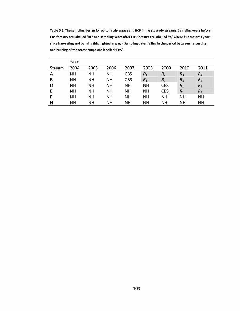
109

Table 5.3. The sampling design for cotton strip assays and BCP in the six study streams. Sampling years before

CBS forestry are labelled ‘NH’ and sampling years after CBS forestry are labelled ‘Rk’ where k represents years

since harvesting and burning (highlighted in grey). Sampling dates falling in the period between harvesting

and burning of the forest coupe are labelled ‘CBS’.

Year

Stream 2004 2005 2006 2007 2008 2009 2010 2011

A NH NH NH CBS R1 R2 R3 R4 B NH NH NH CBS R1 R2 R3 R4 D NH NH NH NH NH CBS R1 R2 E NH NH NH NH NH CBS R1 R2 F NH NH NH NH NH NH NH NH H NH NH NH NH NH NH NH NH

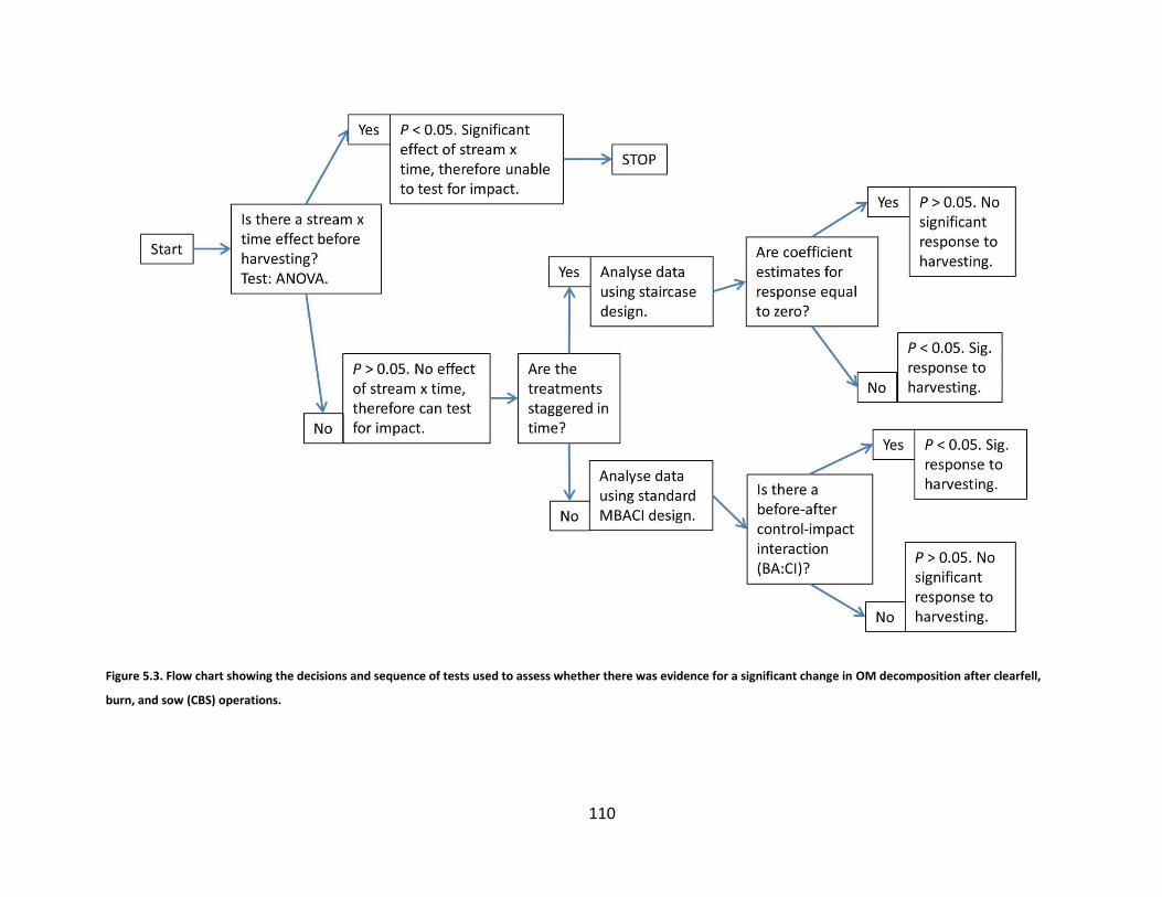
110

Figure 5.3. Flow chart showing the decisions and sequence of tests used to assess whether there was evidence for a significant change in OM decomposition after clearfell,

burn, and sow (CBS) operations.

111

The response variable (either BCP or CSFR) for stream in year t was

analysed using the following linear mixed model:

where – is the estimated mean value of the response variable in the

absence of CBS forestry; is the estimated year effect shared by all

streams independent of whether or not they were subject to CBS forestry; is the

effect of CBS forestry in stream i in year t; is the mean sediment temperature

experienced before sampling; and is the within-stream error assumed

independent for different i, t and independent of the random effects. The random

effects are assumed independent with zero means and variances

and respectively, and these assumptions were checked using standard

procedures (Pinheiro and Bates, 2000). The coefficients for each fixed effect were

tested for significant deviations from 0, with the coefficients for the providing

the test for differences between controls and CBS streams t years after CBS

operations. Positive coefficients indicate the response was elevated relative to

controls, negative values indicated declines. As noted by Walters et al. (1988) tests

for the last two years are less powerful than for the first two years because fewer

streams were available to estimate those coefficients.

Water temperatures showed strong seasonal variation and so periodic terms

(cosine and sine of the proportion of the year expressed in radians) were included in

LMMs. Water temperature data were summarized as the mean, minimum, and

maximum temperatures for each calendar day of the year. The water temperature

for stream at proportional time of the year in year t was analysed using the

following linear mixed model with the trigonometric terms included to fit the

periodic trends in temperature:

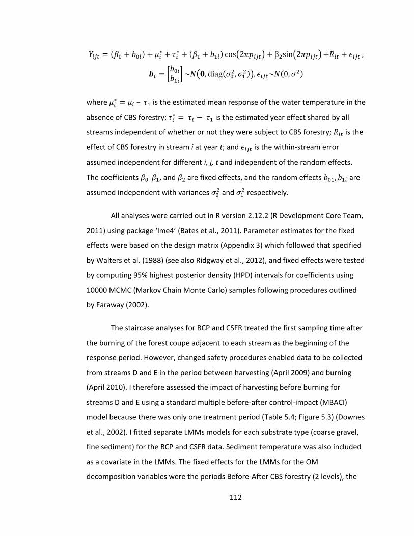
112

( ) ( )

[

] (

)

where – is the estimated mean response of the water temperature in the

absence of CBS forestry; is the estimated year effect shared by all

streams independent of whether or not they were subject to CBS forestry; is the

effect of CBS forestry in stream i at year t; and is the within-stream error

assumed independent for different i, j, t and independent of the random effects.

The coefficients , and are fixed effects, and the random effects are

assumed independent with variances and

respectively.

All analyses were carried out in R version 2.12.2 (R Development Core Team,

2011) using package ‘lme4’ (Bates et al., 2011). Parameter estimates for the fixed

effects were based on the design matrix (Appendix 3) which followed that specified

by Walters et al. (1988) (see also Ridgway et al., 2012), and fixed effects were tested

by computing 95% highest posterior density (HPD) intervals for coefficients using

10000 MCMC (Markov Chain Monte Carlo) samples following procedures outlined

by Faraway (2002).

The staircase analyses for BCP and CSFR treated the first sampling time after

the burning of the forest coupe adjacent to each stream as the beginning of the

response period. However, changed safety procedures enabled data to be collected

from streams D and E in the period between harvesting (April 2009) and burning

(April 2010). I therefore assessed the impact of harvesting before burning for

streams D and E using a standard multiple before-after control-impact (MBACI)

model because there was only one treatment period (Table 5.4; Figure 5.3) (Downes

et al., 2002). I fitted separate LMMs models for each substrate type (coarse gravel,

fine sediment) for the BCP and CSFR data. Sediment temperature was also included

as a covariate in the LMMs. The fixed effects for the LMMs for the OM

decomposition variables were the periods Before-After CBS forestry (2 levels), the

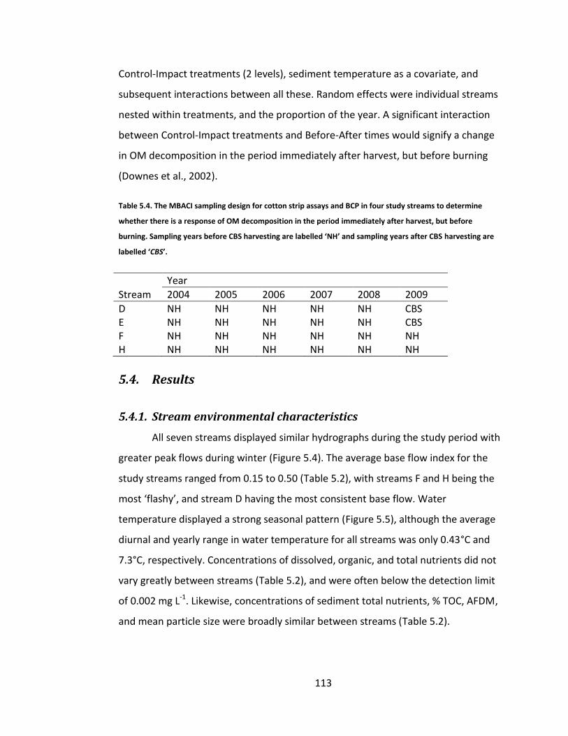
113

Control-Impact treatments (2 levels), sediment temperature as a covariate, and

subsequent interactions between all these. Random effects were individual streams

nested within treatments, and the proportion of the year. A significant interaction

between Control-Impact treatments and Before-After times would signify a change

in OM decomposition in the period immediately after harvest, but before burning

(Downes et al., 2002).

Table 5.4. The MBACI sampling design for cotton strip assays and BCP in four study streams to determine

whether there is a response of OM decomposition in the period immediately after harvest, but before

burning. Sampling years before CBS harvesting are labelled ‘NH’ and sampling years after CBS harvesting are

labelled ‘CBS’.

Year

Stream 2004 2005 2006 2007 2008 2009

D NH NH NH NH NH CBS E NH NH NH NH NH CBS F NH NH NH NH NH NH H NH NH NH NH NH NH

5.4. Results

5.4.1. Stream environmental characteristics

All seven streams displayed similar hydrographs during the study period with

greater peak flows during winter (Figure 5.4). The average base flow index for the

study streams ranged from 0.15 to 0.50 (Table 5.2), with streams F and H being the

most ‘flashy’, and stream D having the most consistent base flow. Water

temperature displayed a strong seasonal pattern (Figure 5.5), although the average

diurnal and yearly range in water temperature for all streams was only 0.43°C and

7.3°C, respectively. Concentrations of dissolved, organic, and total nutrients did not

vary greatly between streams (Table 5.2), and were often below the detection limit

of 0.002 mg L-1. Likewise, concentrations of sediment total nutrients, % TOC, AFDM,

and mean particle size were broadly similar between streams (Table 5.2).

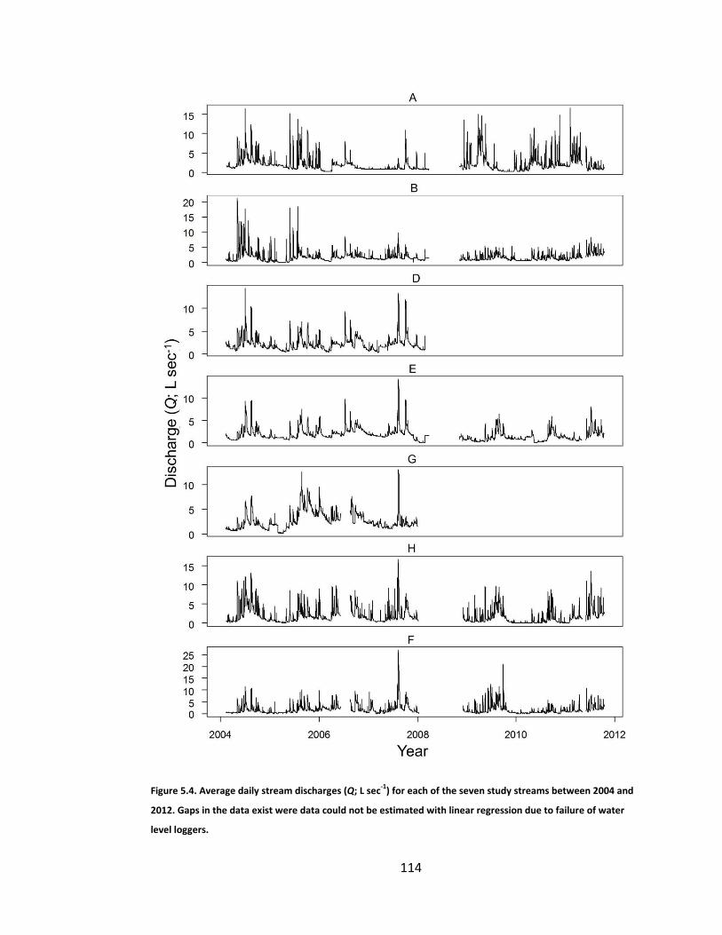
114

Figure 5.4. Average daily stream discharges (Q; L sec-1

) for each of the seven study streams between 2004 and

2012. Gaps in the data exist were data could not be estimated with linear regression due to failure of water

level loggers.

115

Figure 5.5. Average daily stream temperatures (°C) for each of the seven study streams between 2004 and

2012. Gaps in the data exist due to failure of temperature loggers. Vertical lines represent the harvest (red)

and burn (brown) dates for harvested streams.

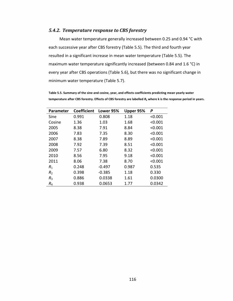
116

5.4.2. Temperature response to CBS forestry

Mean water temperature generally increased between 0.25 and 0.94 °C with

each successive year after CBS forestry (Table 5.5). The third and fourth year

resulted in a significant increase in mean water temperature (Table 5.5). The

maximum water temperature significantly increased (between 0.84 and 1.6 °C) in

every year after CBS operations (Table 5.6), but there was no significant change in

minimum water temperature (Table 5.7).

Table 5.5. Summary of the sine and cosine, year, and effects coefficients predicting mean yearly water

temperature after CBS forestry. Effects of CBS forestry are labelled Rk where k is the response period in years.

Parameter Coefficient Lower 95% Upper 95% P

Sine 0.991 0.808 1.18 <0.001 Cosine 1.36 1.03 1.68 <0.001 2005 8.38 7.91 8.84 <0.001 2006 7.83 7.35 8.30 <0.001 2007 8.38 7.89 8.89 <0.001 2008 7.92 7.39 8.51 <0.001 2009 7.57 6.80 8.32 <0.001 2010 8.56 7.95 9.18 <0.001 2011 8.06 7.38 8.70 <0.001 R1 0.248 -0.497 0.987 0.535 R2 0.398 -0.385 1.18 0.330 R3 0.886 0.0338 1.61 0.0300 R4 0.938 0.0653 1.77 0.0342

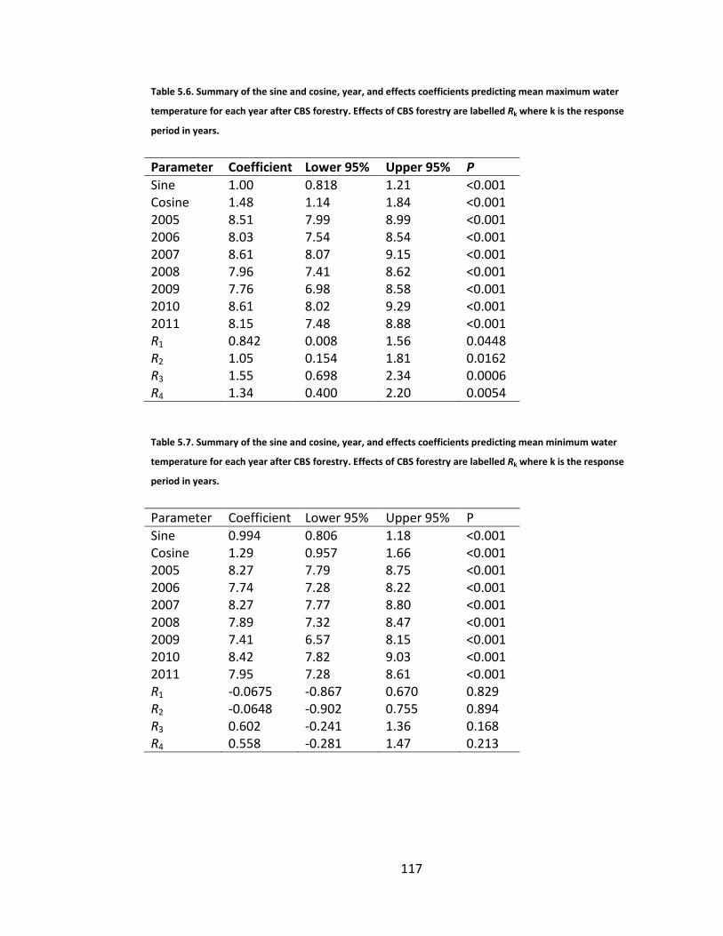
117

Table 5.6. Summary of the sine and cosine, year, and effects coefficients predicting mean maximum water

temperature for each year after CBS forestry. Effects of CBS forestry are labelled Rk where k is the response

period in years.


Sine 1.00 0.818 1.21 <0.001 Cosine 1.48 1.14 1.84 <0.001 2005 8.51 7.99 8.99 <0.001 2006 8.03 7.54 8.54 <0.001 2007 8.61 8.07 9.15 <0.001 2008 7.96 7.41 8.62 <0.001 2009 7.76 6.98 8.58 <0.001 2010 8.61 8.02 9.29 <0.001 2011 8.15 7.48 8.88 <0.001 R1 0.842 0.008 1.56 0.0448 R2 1.05 0.154 1.81 0.0162 R3 1.55 0.698 2.34 0.0006 R4 1.34 0.400 2.20 0.0054

Table 5.7. Summary of the sine and cosine, year, and effects coefficients predicting mean minimum water

temperature for each year after CBS forestry. Effects of CBS forestry are labelled Rk where k is the response

period in years.


Sine 0.994 0.806 1.18 <0.001 Cosine 1.29 0.957 1.66 <0.001 2005 8.27 7.79 8.75 <0.001 2006 7.74 7.28 8.22 <0.001 2007 8.27 7.77 8.80 <0.001 2008 7.89 7.32 8.47 <0.001 2009 7.41 6.57 8.15 <0.001 2010 8.42 7.82 9.03 <0.001 2011 7.95 7.28 8.61 <0.001 R1 -0.0675 -0.867 0.670 0.829 R2 -0.0648 -0.902 0.755 0.894 R3 0.602 -0.241 1.36 0.168 R4 0.558 -0.281 1.47 0.213

118

5.4.3. Response of cotton strip decomposition to CBS forestry

The average CSFR varied from 0.32 to 0.96 (interquartile range: 0.67 to 0.86)

in coarse gravel sediment (Figure 5.6) and 0.38 to 0.98 (interquartile range: 0.72 to

0.85) in fine sediment (Figure 5.7). The response in cotton strip decomposition to

CBS forestry differed between benthic habitats. In coarse gravel sediment there was

evidence for a decrease (i.e. an increase in CSFR) in cellulose decomposition due to

CBS forestry (Table 5.8). However, this negative effect was not apparent until the

second year after burning (R2 in Table 5.8), with the effect weakening in the third

year but becoming stronger in the fourth year. In contrast, there were no detectable

effects of CBS forestry in fine sediments (Table 5.9).

The collection of CTFR data for streams D and E in the period between

harvesting (April 2009) and burning (April 2010) allowed the short-term (1 year)

assessment of the impact of tree removal before burning. There was, however, no

detectable effect of harvesting on cotton strip decomposition in this short period

before burning in coarse gravel and fine sediment habitat (BA × CI P-values > 0.3).

When pooled across all streams and times, cotton strip decomposition was not

correlated with sediment temperature in coarse gravel (R2 = 0.007, P = 0.3) or fine

sediment (R2 = 0.003, P = 0.5) (Figure 5.8).

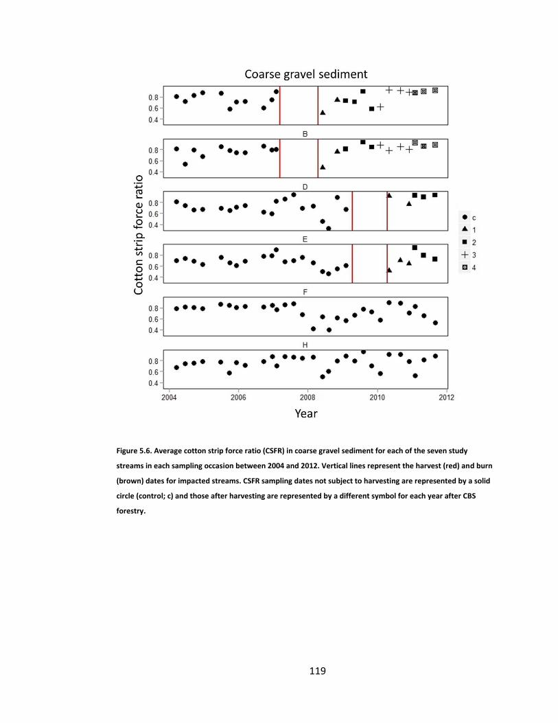
119

Figure 5.6. Average cotton strip force ratio (CSFR) in coarse gravel sediment for each of the seven study

streams in each sampling occasion between 2004 and 2012. Vertical lines represent the harvest (red) and burn

(brown) dates for impacted streams. CSFR sampling dates not subject to harvesting are represented by a solid

circle (control; c) and those after harvesting are represented by a different symbol for each year after CBS

forestry.

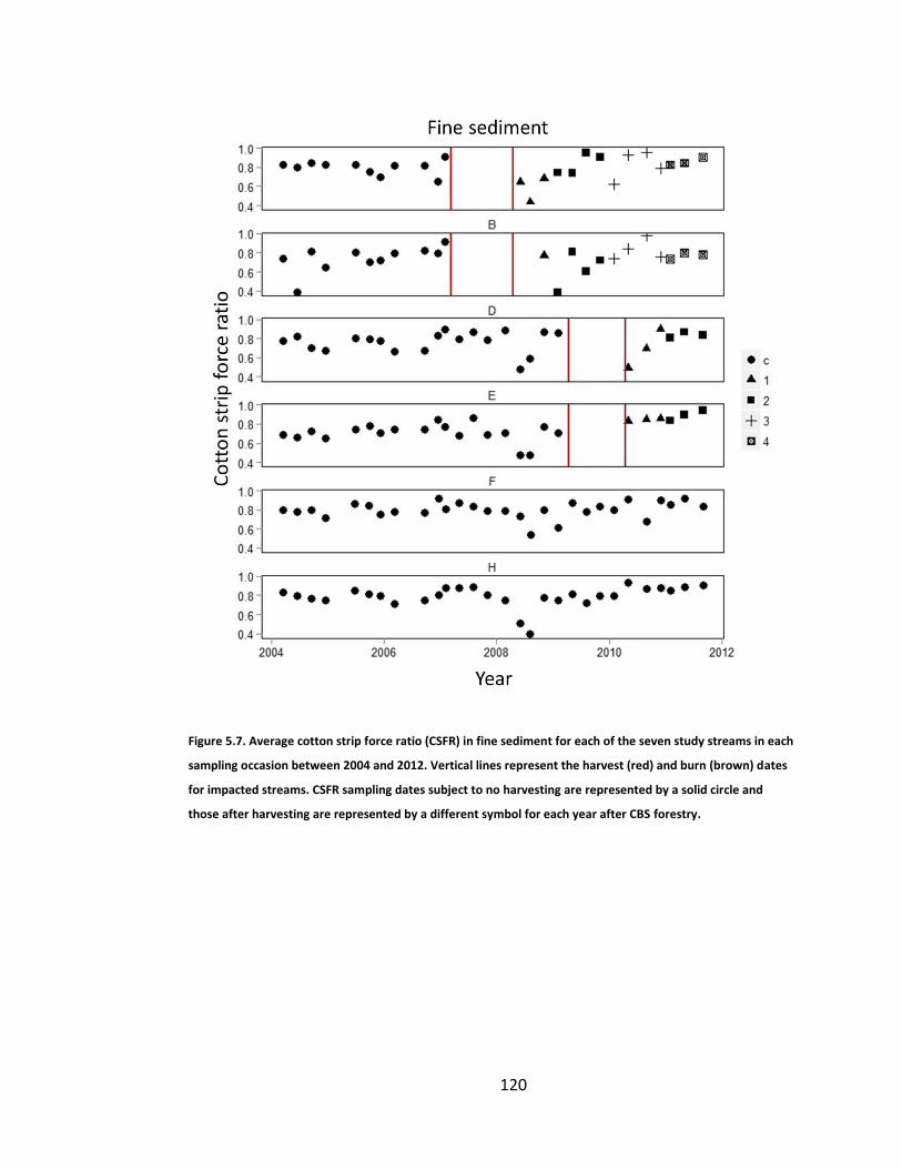
120

Figure 5.7. Average cotton strip force ratio (CSFR) in fine sediment for each of the seven study streams in each

sampling occasion between 2004 and 2012. Vertical lines represent the harvest (red) and burn (brown) dates

for impacted streams. CSFR sampling dates subject to no harvesting are represented by a solid circle and

those after harvesting are represented by a different symbol for each year after CBS forestry.

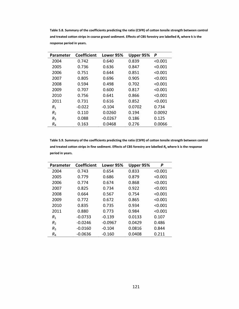
121

Table 5.8. Summary of the coefficients predicting the ratio (CSFR) of cotton tensile strength between control

and treated cotton strips in coarse gravel sediment. Effects of CBS forestry are labelled Rk where k is the

response period in years.


2004 0.742 0.640 0.839 <0.001 2005 0.736 0.636 0.847 <0.001 2006 0.751 0.644 0.851 <0.001 2007 0.805 0.696 0.905 <0.001 2008 0.594 0.498 0.702 <0.001 2009 0.707 0.600 0.817 <0.001 2010 0.756 0.641 0.866 <0.001 2011 0.731 0.616 0.852 <0.001 R1 -0.022 -0.104 0.0702 0.734 R2 0.110 0.0260 0.194 0.0092 R3 0.088 -0.0267 0.186 0.125 R4 0.163 0.0468 0.276 0.0066

Table 5.9. Summary of the coefficients predicting the ratio (CSFR) of cotton tensile strength between control

and treated cotton strips in fine sediment. Effects of CBS forestry are labelled Rk where k is the response

period in years.


2004 0.743 0.654 0.833 <0.001 2005 0.779 0.686 0.879 <0.001 2006 0.774 0.674 0.868 <0.001 2007 0.825 0.734 0.922 <0.001 2008 0.664 0.567 0.754 <0.001 2009 0.772 0.672 0.865 <0.001 2010 0.835 0.735 0.934 <0.001 2011 0.880 0.773 0.984 <0.001 R1 -0.0733 -0.139 0.0133 0.107 R2 -0.0246 -0.0967 0.0429 0.486 R3 -0.0160 -0.104 0.0816 0.844 R4 -0.0636 -0.160 0.0408 0.211

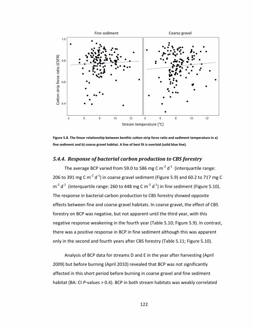
122

Figure 5.8. The linear relationship between benthic cotton strip force ratio and sediment temperature in a)

fine sediment and b) coarse gravel habitat. A line of best fit is overlaid (solid blue line).

5.4.4. Response of bacterial carbon production to CBS forestry

The average BCP varied from 59.0 to 586 mg C m-2 d-1 (interquartile range:

206 to 391 mg C m-2 d-1) in coarse gravel sediment (Figure 5.9) and 60.2 to 717 mg C

m-2 d-1 (interquartile range: 260 to 448 mg C m-2 d-1) in fine sediment (Figure 5.10).

The response in bacterial carbon production to CBS forestry showed opposite

effects between fine and coarse gravel habitats. In coarse gravel, the effect of CBS

forestry on BCP was negative, but not apparent until the third year, with this

negative response weakening in the fourth year (Table 5.10; Figure 5.9). In contrast,

there was a positive response in BCP in fine sediment although this was apparent

only in the second and fourth years after CBS forestry (Table 5.11; Figure 5.10).

Analysis of BCP data for streams D and E in the year after harvesting (April

2009) but before burning (April 2010) revealed that BCP was not significantly

affected in this short period before burning in coarse gravel and fine sediment

habitat (BA: CI P-values > 0.4). BCP in both stream habitats was weakly correlated

123

with sediment temperature (Figure 5.11), but the correlation was stronger in coarse

gravel (R2 = 0.15, P < 0.001) than fine sediment habitat (R2 = 0.04, P= 0.01).

Figure 5.9. Average BCP in coarse gravel sediment for each of the seven study streams in each sampling

occasion between 2004 and 2012. Vertical lines represent the harvest (red) and burn (brown) dates for

impacted streams. BCP sampling dates subject to no harvesting are represented by a solid circle and those

after harvesting are represented by a different symbol for each year after CBS forestry.

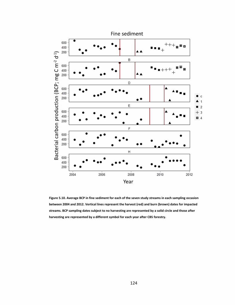
124

Figure 5.10. Average BCP in fine sediment for each of the seven study streams in each sampling occasion

between 2004 and 2012. Vertical lines represent the harvest (red) and burn (brown) dates for impacted

streams. BCP sampling dates subject to no harvesting are represented by a solid circle and those after

harvesting are represented by a different symbol for each year after CBS forestry.

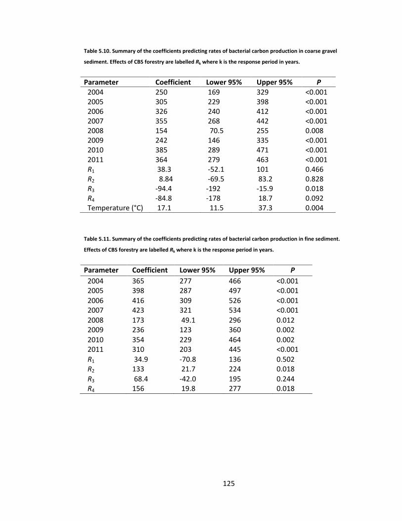
125

Table 5.10. Summary of the coefficients predicting rates of bacterial carbon production in coarse gravel

sediment. Effects of CBS forestry are labelled Rk where k is the response period in years.


2004 250 169 329 <0.001 2005 305 229 398 <0.001 2006 326 240 412 <0.001 2007 355 268 442 <0.001 2008 154 70.5 255 0.008 2009 242 146 335 <0.001 2010 385 289 471 <0.001 2011 364 279 463 <0.001 R1 38.3 -52.1 101 0.466 R2 8.84 -69.5 83.2 0.828 R3 -94.4 -192 -15.9 0.018 R4 -84.8 -178 18.7 0.092 Temperature (°C) 17.1 11.5 37.3 0.004

Table 5.11. Summary of the coefficients predicting rates of bacterial carbon production in fine sediment.

Effects of CBS forestry are labelled Rk where k is the response period in years.


2004 365 277 466 <0.001 2005 398 287 497 <0.001

2006 416 309 526 <0.001 2007 423 321 534 <0.001

2008 173 49.1 296 0.012 2009 236 123 360 0.002

2010 354 229 464 0.002 2011 310 203 445 <0.001

R1 34.9 -70.8 136 0.502 R2 133 21.7 224 0.018

R3 68.4 -42.0 195 0.244 R4 156 19.8 277 0.018

126

Figure 5.11. The linear relationship between benthic bacterial carbon production (BCP; mg C m-2

d-1

) and

sediment temperature in a) fine sediment and b) coarse gravel habitat. A line of best fit is overlaid (solid blue

line).

5.5. Discussion

5.5.1. Elevated water temperature after CBS forestry

In the first 4 years after harvest, CBS forestry raised daily mean and

maximum water temperatures, with the magnitudes of the changes similar to those

found in other temperate forested headwater streams impacted by clearfell

harvesting (Johnson and Jones, 2000; Moore et al., 2005; Gomi et al., 2006b). These

changes are likely a direct consequence of the large reduction in stream canopy

cover after CBS forestry (Clapcott and Barmuta, 2010) because decreased shading

and increased solar radiation to the stream channel are key mechanisms elevating

stream temperature after clearfelling (Johnson and Jones, 2000; Groom et al.,

2011). Interestingly, increases in mean water temperature were not significant in

the first and second year after CBS forestry. It is possible that the large amounts of

logging slash (i.e. leaves, branches, bark, and wood) put into the stream channel

during CBS operations (see Chapter 2) moderated any immediate temperature

127

increases by shading the stream (Jackson et al., 2001; Janisch et al., 2012). However,

by the third year after CBS operations much of the smaller logging slash (i.e. leaves,

braches, and bark) may have been transported downstream because CBS-affected

headwater streams retain less fine material than old-growth streams (Watson and

Barmuta, 2010). The reduced covering of finer material could have increased the

amount of light reaching the stream surface, subsequently elevating the water

temperature.

5.5.2. Contrasting response of OM decomposition to CBS forestry

The response of OM decomposition to CBS forestry differed between years

and among benthic habitats. Benthic habitats in small, headwater streams are

strongly influenced by external factors (such as sediment transport and deposition)

and consequently their distribution and characteristics are highly heterogeneous

over space and time (Vannote et al., 1980; Gooderham et al., 2007; Clapcott and

Barmuta, 2009). Therefore, it is not surprising that the response of OM

decomposition to CBS forestry was also heterogeneous in space and time.

Generally, there was either a modest reduction or no change in OM

processing in the four years after harvesting, with only BCP in fine sediments

displaying a significant increase in the third year after harvesting. Research in similar

sized streams in Canadian boreal forests also found no effect of clearcutting on

microbial decomposition of OM (Kreutzweiser et al., 2008; Kreutzweiser et al.,

2010): although harvesting practices is this region had substantially larger riparian

buffers (Table 5.12). The findings in my study are, however, opposite to the

expectations generated from previous space-for-time surveys in these streams

which found greater BCP and CTFR in coarse gravel and fine sediments less than five

years after CBS forestry (Clapcott, 2007; Clapcott and Barmuta, 2010). These

contrasting findings may be because, unlike the MBACI study, the space-for-time

surveys did not account for the spatial and temporal heterogeneity that exists in

these streams. For instance, this MBACI study showed that the variability in CTFR

128

after CBS forestry in fine sediments was no different from that prior to operations

(Table 5.9). However, space-for-time surveys do not account for this temporal

variability, and therefore any observed response cannot be solely attributed to the

disturbance itself but also to variation that occurs naturally (Downes et al., 2002).

Greater OM decomposition was expected after CBS operations because of

elevated stream temperatures which have previously been found to increase the

activity of benthic bacteria, fungi and invertebrates (González and Graça, 2003;

Dang et al., 2009; Clapcott and Barmuta, 2010; Ferreira and Chauvet, 2011a).

Surprisingly, stream temperature in this study was not related to cotton strip

decomposition and was only weakly correlated with rates of BCP in coarse gravel

sediment (Figure 5.8; Figure 5.11). While temperature is commonly viewed as a

major factor influencing ecosystem processes in streams (Bergfur et al., 2007; Young

et al., 2008), the average water temperature range in this study (diurnal range =

0.43°C and yearly range = 7.3°C) was much narrower than most studies that

document the importance of temperature (González and Graça, 2003; Dang et al.,

2009; Ferreira and Chauvet, 2011a). Furthermore, several studies have

demonstrated that variations in other environmental variables (e.g. stream flow,

dissolved nutrients and seasonality in OM inputs) are better correlated with rates of

OM decomposition than water temperature at both local (Benstead and Huryn,

2011; Pozo et al., 2011) and regional scales (Pérez et al., 2011). The source of DOM

may have been more influential in determining OM decomposition than water

temperature in the study streams, because variation in DOM source was shown in

Chapter 4 to better describe rates of BCP than variation in water temperature.

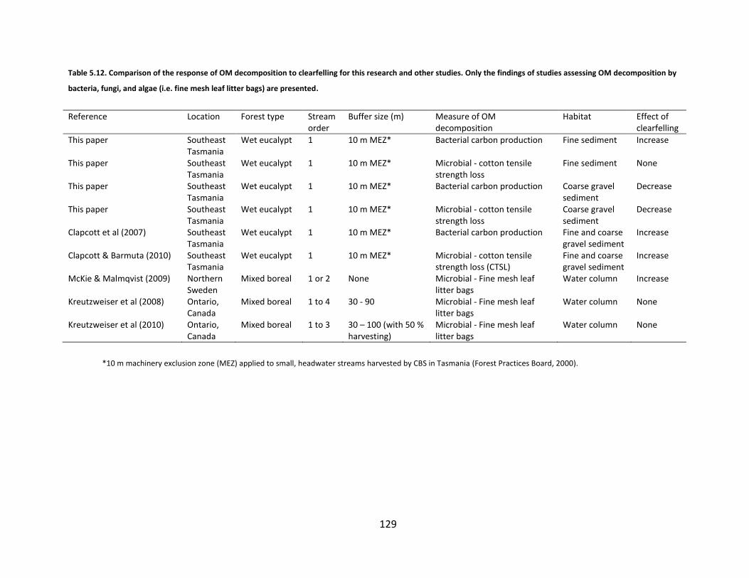
129

Table 5.12. Comparison of the response of OM decomposition to clearfelling for this research and other studies. Only the findings of studies assessing OM decomposition by

bacteria, fungi, and algae (i.e. fine mesh leaf litter bags) are presented.

Reference Location Forest type Stream order

Buffer size (m) Measure of OM decomposition

Habitat Effect of clearfelling

This paper Southeast Tasmania

Wet eucalypt 1 10 m MEZ* Bacterial carbon production Fine sediment Increase


Wet eucalypt 1 10 m MEZ* Microbial - cotton tensile strength loss

Fine sediment None


Wet eucalypt 1 10 m MEZ* Bacterial carbon production Coarse gravel sediment

Decrease


Wet eucalypt 1 10 m MEZ* Microbial - cotton tensile strength loss

Coarse gravel sediment

Decrease

Clapcott et al (2007) Southeast Tasmania

Wet eucalypt 1 10 m MEZ* Bacterial carbon production Fine and coarse gravel sediment

Increase

Clapcott & Barmuta (2010) Southeast Tasmania

Wet eucalypt 1 10 m MEZ* Microbial - cotton tensile strength loss (CTSL)

Fine and coarse gravel sediment

Increase

McKie & Malmqvist (2009) Northern Sweden

Mixed boreal 1 or 2 None Microbial - Fine mesh leaf litter bags

Water column Increase

Kreutzweiser et al (2008) Ontario, Canada

Mixed boreal 1 to 4 30 - 90 Microbial - Fine mesh leaf litter bags

Water column None

Kreutzweiser et al (2010) Ontario, Canada

Mixed boreal 1 to 3 30 – 100 (with 50 % harvesting)

Microbial - Fine mesh leaf litter bags

Water column None

*10 m machinery exclusion zone (MEZ) applied to small, headwater streams harvested by CBS in Tasmania (Forest Practices Board, 2000).

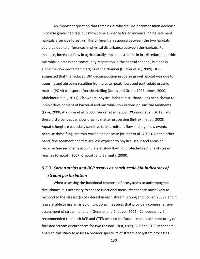
130

An important question that remains is: why did OM decomposition decrease

in coarse gravel habitats but show some evidence for an increase in fine sediment

habitats after CBS forestry? This differential response between the two habitats

could be due to differences in physical disturbance between the habitats. For

instance, increased flow in agriculturally impacted streams in Brazil reduced benthic

microbial biomass and community respiration in the central channel, but not in

along the flow-protected margins of the channel (Gücker et al., 2009). It is

suggested that the reduced OM decomposition in coarse gravel habitat was due to

scouring and abrading resulting from greater peak flows and particulate organic

matter (POM) transport after clearfelling (Jones and Grant, 1996; Jones, 2000;

Abdelnour et al., 2011). Elsewhere, physical habitat disturbance has been shown to

inhibit development of bacterial and microbial populations on surficial sediments

(Lake, 2000; Atkinson et al., 2008; Gücker et al., 2009; O'Connor et al., 2012), and

these disturbances can slow organic matter processing (Entrekin et al., 2008).

Aquatic fungi are especially sensitive to intermittent flow and high flow events

because these fungi are thin-walled and delicate (Bruder et al., 2011). On the other

hand, fine sediment habitats are less exposed to physical scour and abrasion

because fine sediments accumulate at slow flowing, protected sections of stream

reaches (Clapcott, 2007; Clapcott and Barmuta, 2009).

5.5.3. Cotton strips and BCP assays as reach-scale bio-indicators of

stream perturbation

When assessing the functional response of ecosystems to anthropogenic

disturbance it is necessary to choose functional measures that are most likely to

respond to the stressor(s) of interest in each stream (Young and Collier, 2009), and it

is preferable to use an array of functional measures that provide a comprehensive

assessment of stream function (Gessner and Chauvet, 2002). Consequently, I

recommended that both BCP and CTFR be used for future reach-scale monitoring of

forested stream disturbances for two reasons. First, using BCP and CTFR in tandem

enabled this study to assess a broader spectrum of stream ecosystem processes

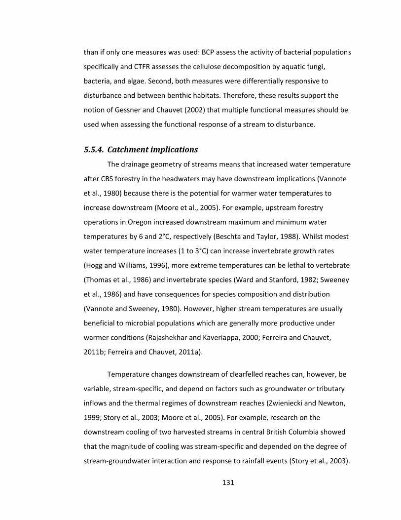
131

than if only one measures was used: BCP assess the activity of bacterial populations

specifically and CTFR assesses the cellulose decomposition by aquatic fungi,

bacteria, and algae. Second, both measures were differentially responsive to

disturbance and between benthic habitats. Therefore, these results support the

notion of Gessner and Chauvet (2002) that multiple functional measures should be

used when assessing the functional response of a stream to disturbance.

5.5.4. Catchment implications

The drainage geometry of streams means that increased water temperature

after CBS forestry in the headwaters may have downstream implications (Vannote

et al., 1980) because there is the potential for warmer water temperatures to

increase downstream (Moore et al., 2005). For example, upstream forestry

operations in Oregon increased downstream maximum and minimum water

temperatures by 6 and 2°C, respectively (Beschta and Taylor, 1988). Whilst modest

water temperature increases (1 to 3°C) can increase invertebrate growth rates

(Hogg and Williams, 1996), more extreme temperatures can be lethal to vertebrate

(Thomas et al., 1986) and invertebrate species (Ward and Stanford, 1982; Sweeney

et al., 1986) and have consequences for species composition and distribution

(Vannote and Sweeney, 1980). However, higher stream temperatures are usually

beneficial to microbial populations which are generally more productive under

warmer conditions (Rajashekhar and Kaveriappa, 2000; Ferreira and Chauvet,

2011b; Ferreira and Chauvet, 2011a).

Temperature changes downstream of clearfelled reaches can, however, be

variable, stream-specific, and depend on factors such as groundwater or tributary

inflows and the thermal regimes of downstream reaches (Zwieniecki and Newton,

1999; Story et al., 2003; Moore et al., 2005). For example, research on the

downstream cooling of two harvested streams in central British Columbia showed

that the magnitude of cooling was stream-specific and depended on the degree of

stream-groundwater interaction and response to rainfall events (Story et al., 2003).

132

Variability in the shading of downstream reaches may also contribute to

temperature changes. For example, research on five 2nd order Australian streams

showed that large changes in riparian cover (40 to 70%) over just 600m of channel

led to 4°C increases in stream temperature (Rutherford et al., 2004). Clearly,

building predictive models for downstream changes in thermal regimes will require

better, stream- and catchment-specific information on groundwater and tributary

inflows as well as calibrated modelling of riparian shading.

Similarly, alterations to OM decomposition in headwaters may also have

implications for downstream ecosystems, but the potentially differential responses

between headwater habitats may inhibit attempts to predict quantitatively these

cumulative effects. For instance, reduced OM decomposition in coarse gravel

habitat may lead to an increased export downstream of unprocessed CPOM,

especially given that CBS-affected reaches retain less CPOM than undisturbed

streams (Watson and Barmuta, 2010). This may have negative consequences for

the abundance and diversity of aquatic macroinvertebrates because many aquatic

macroinvertebrates feed on CPOM which is made more palatable by microbial

processes (Bunn, 1988; Pozo et al., 1998). On the other hand, more rapid OM

decomposition in fine sediments may represent a more rapid transfer of energy

through detrital pathways as was observed in clearcut Scandinavian streams (McKie

and Malmqvist, 2009), and possibly increase the export of more processed OM from

this habitat. Scaling up the habitat-specific responses will not only require estimates

of the relative abundances of the distinct habitats, but may also require research

into how different spatial configurations of habitats may affect reach- and

catchment-scale estimates of microbial activity and decomposition (Levin, 1992).

While this study detected short-term (<4 years) responses of OM

decomposition to CBS forestry, an important question remains: is the magnitude of

the response ecologically important? It is possible that the changes to OM

decomposition caused by CBS forestry may not affect the energy transfer in the

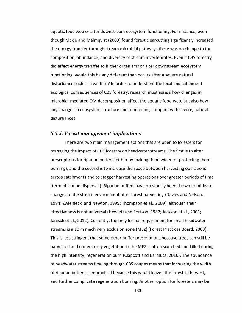
133

aquatic food web or alter downstream ecosystem functioning. For instance, even

though Mckie and Malmqvist (2009) found forest clearcutting significantly increased

the energy transfer through stream microbial pathways there was no change to the

composition, abundance, and diversity of stream invertebrates. Even if CBS forestry

did affect energy transfer to higher organisms or alter downstream ecosystem

functioning, would this be any different than occurs after a severe natural

disturbance such as a wildfire? In order to understand the local and catchment

ecological consequences of CBS forestry, research must assess how changes in

microbial-mediated OM decomposition affect the aquatic food web, but also how

any changes in ecosystem structure and functioning compare with severe, natural

disturbances.

5.5.5. Forest management implications

There are two main management actions that are open to foresters for

managing the impact of CBS forestry on headwater streams. The first is to alter

prescriptions for riparian buffers (either by making them wider, or protecting them

burning), and the second is to increase the space between harvesting operations

across catchments and to stagger harvesting operations over greater periods of time

(termed ‘coupe dispersal’). Riparian buffers have previously been shown to mitigate

changes to the stream environment after forest harvesting (Davies and Nelson,

1994; Zwieniecki and Newton, 1999; Thompson et al., 2009), although their

effectiveness is not universal (Hewlett and Fortson, 1982; Jackson et al., 2001;

Janisch et al., 2012). Currently, the only formal requirement for small headwater

streams is a 10 m machinery exclusion zone (MEZ) (Forest Practices Board, 2000).

This is less stringent that some other buffer prescriptions because trees can still be

harvested and understorey vegetation in the MEZ is often scorched and killed during

the high intensity, regeneration burn (Clapcott and Barmuta, 2010). The abundance

of headwater streams flowing through CBS coupes means that increasing the width

of riparian buffers is impractical because this would leave little forest to harvest,

and further complicate regeneration burning. Another option for foresters may be

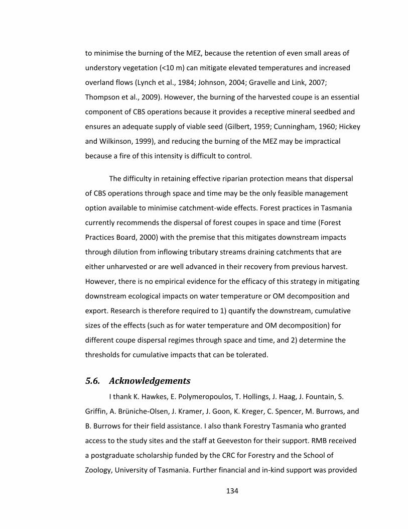
134

to minimise the burning of the MEZ, because the retention of even small areas of

understory vegetation (<10 m) can mitigate elevated temperatures and increased

overland flows (Lynch et al., 1984; Johnson, 2004; Gravelle and Link, 2007;

Thompson et al., 2009). However, the burning of the harvested coupe is an essential

component of CBS operations because it provides a receptive mineral seedbed and

ensures an adequate supply of viable seed (Gilbert, 1959; Cunningham, 1960; Hickey

and Wilkinson, 1999), and reducing the burning of the MEZ may be impractical

because a fire of this intensity is difficult to control.

The difficulty in retaining effective riparian protection means that dispersal

of CBS operations through space and time may be the only feasible management

option available to minimise catchment-wide effects. Forest practices in Tasmania

currently recommends the dispersal of forest coupes in space and time (Forest

Practices Board, 2000) with the premise that this mitigates downstream impacts

through dilution from inflowing tributary streams draining catchments that are

either unharvested or are well advanced in their recovery from previous harvest.

However, there is no empirical evidence for the efficacy of this strategy in mitigating

downstream ecological impacts on water temperature or OM decomposition and

export. Research is therefore required to 1) quantify the downstream, cumulative

sizes of the effects (such as for water temperature and OM decomposition) for

different coupe dispersal regimes through space and time, and 2) determine the

thresholds for cumulative impacts that can be tolerated.

5.6. Acknowledgements

I thank K. Hawkes, E. Polymeropoulos, T. Hollings, J. Haag, J. Fountain, S.

Griffin, A. Brüniche-Olsen, J. Kramer, J. Goon, K. Kreger, C. Spencer, M. Burrows, and

B. Burrows for their field assistance. I also thank Forestry Tasmania who granted

access to the study sites and the staff at Geeveston for their support. RMB received

a postgraduate scholarship funded by the CRC for Forestry and the School of

Zoology, University of Tasmania. Further financial and in-kind support was provided

135

by the Forest Practices Authority Tasmania and School of Zoology at the University

of Tasmania. Dr S. Munks (Forest Practices Authority), Professor P.E. Davies

(University of Tasmania) and Dr. S. Roberts (Forestry Tasmania) provided comments

and advice throughout the project.

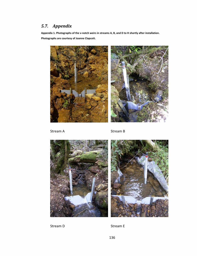
136

5.7. Appendix

Appendix 1. Photographs of the v-notch weirs in streams A, B, and D to H shortly after installation.

Photographs are courtesy of Joanne Clapcott.

Stream A Stream B

Stream D Stream E

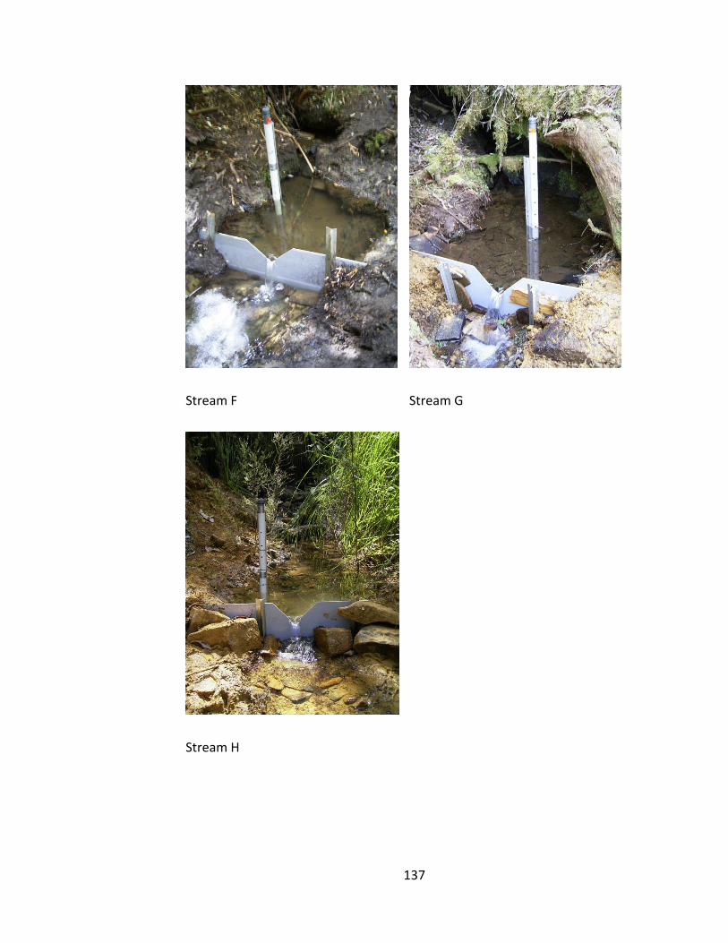
137

Stream F Stream G

Stream H

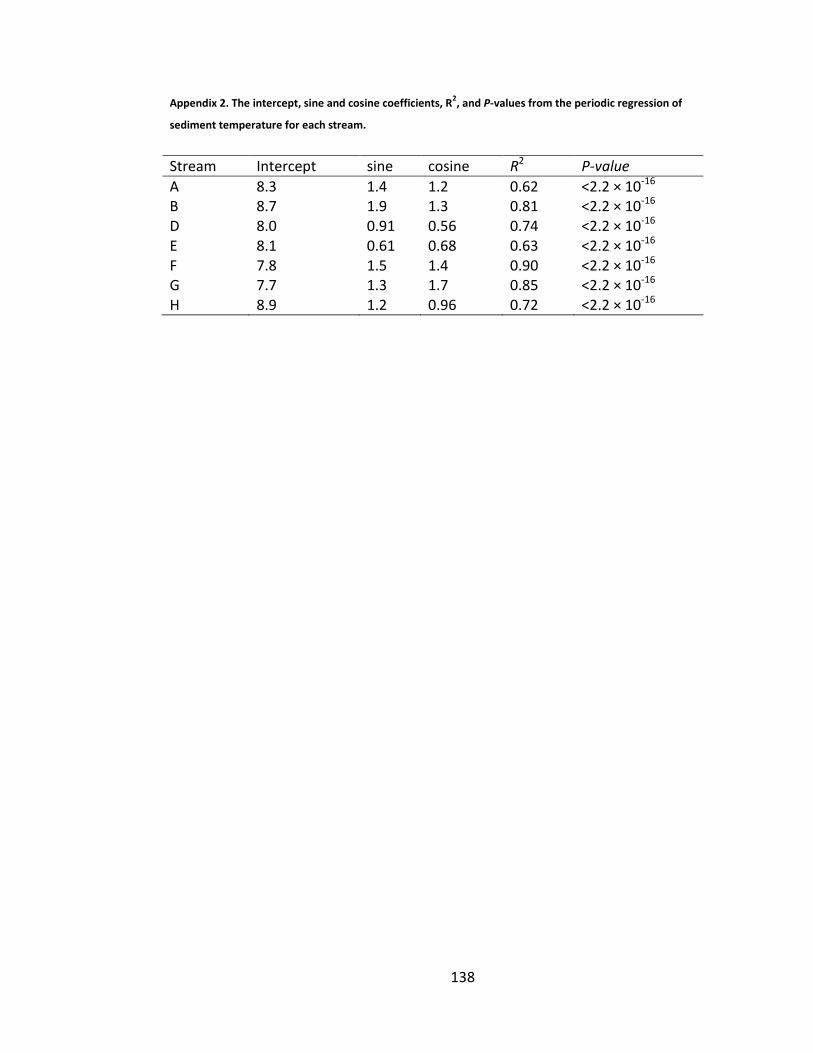
138

Appendix 2. The intercept, sine and cosine coefficients, R2, and P-values from the periodic regression of

sediment temperature for each stream.

Stream Intercept sine cosine R2 P-value

A 8.3 1.4 1.2 0.62 <2.2 × 10-16 B 8.7 1.9 1.3 0.81 <2.2 × 10-16 D 8.0 0.91 0.56 0.74 <2.2 × 10-16 E 8.1 0.61 0.68 0.63 <2.2 × 10-16 F 7.8 1.5 1.4 0.90 <2.2 × 10-16 G 7.7 1.3 1.7 0.85 <2.2 × 10-16 H 8.9 1.2 0.96 0.72 <2.2 × 10-16

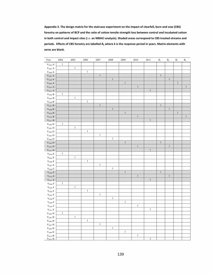
139

Appendix 3. The design matrix for the staircase experiment on the impact of clearfell, burn and sow (CBS)

forestry on patterns of BCP and the ratio of cotton tensile strength loss between control and incubated cotton

in both control and impact sites (i.e. an MBACI analysis). Shaded areas correspond to CBS treated streams and

periods. Effects of CBS forestry are labelled Rk where k is the response period in years. Matrix elements with

zeros are blank.

Year 2004 2005 2006 2007 2008 2009 2010 2011 R1 R2 R3 R4

Y2004 A 1

Y2005 A 1

Y2006 A 1

Y2007 A 1 1

Y2008 A 1 1

Y2009 A 1 1

Y2010 A 1 1

Y2011 A 1

Y2004 B 1

Y2005 B 1

Y2006 B 1

Y2007 B 1 1

Y2008 B 1 1

Y2009 B 1 1

Y2010 B 1 1

Y2011 B 1

Y2004 D 1

Y2005 D 1

Y2006 D 1

Y2007 D 1

Y2008 D 1

Y2009 D 1 1

Y2010 D 1 1

Y2011 D 1

Y2004 E 1

Y2005 E 1

Y2006 E 1

Y2007 E 1

Y2008 E 1

Y2009 E 1 1

Y2010 E 1 1

Y2011 E 1

Y2004 F 1

Y2005 F 1

Y2006 F 1

Y2007 F 1

Y2008 F 1

Y2009 F 1

Y2010 F 1

Y2011 F 1

Y2004 H 1

Y2005 H 1

Y2006 H 1

Y2007 H 1

Y2008 H 1

Y2009 H 1

Y2010 H 1

Y2011 H 1

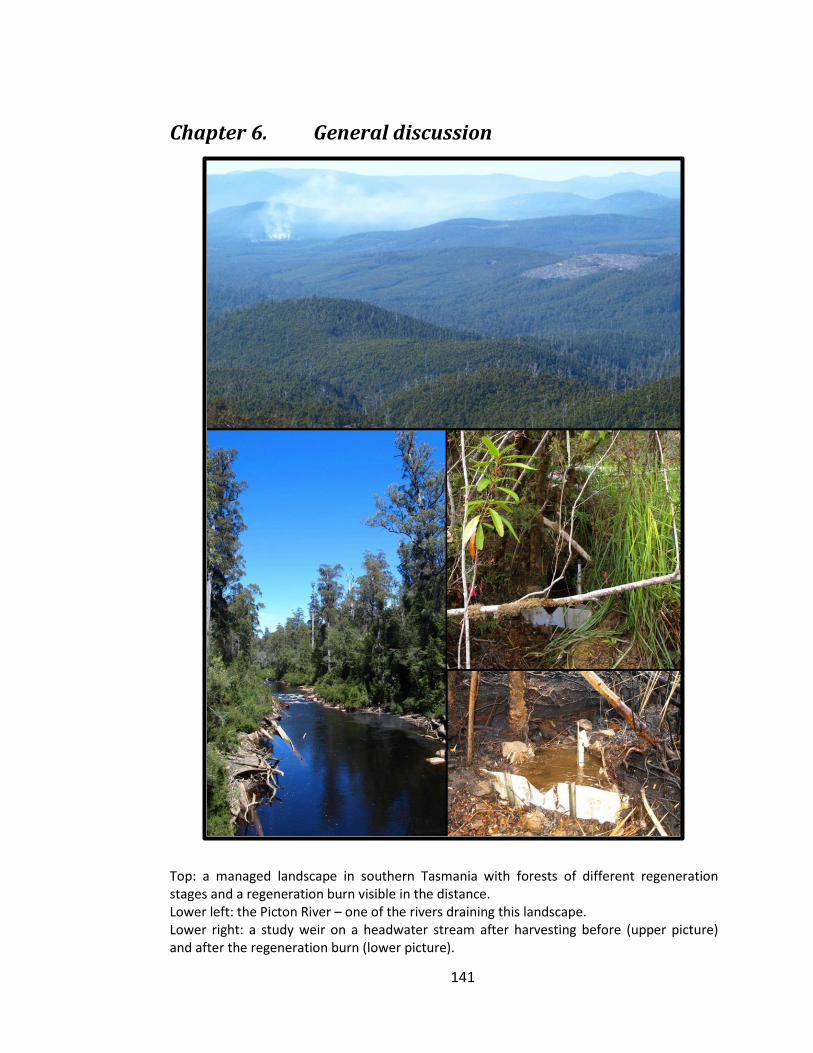
141

Chapter 6. General discussion

Top: a managed landscape in southern Tasmania with forests of different regeneration stages and a regeneration burn visible in the distance. Lower left: the Picton River – one of the rivers draining this landscape. Lower right: a study weir on a headwater stream after harvesting before (upper picture) and after the regeneration burn (lower picture).

142

6.1. Synthesis - The effect of CBS forestry on the structure and

function of southern Tasmanian headwater streams

I investigated the impact of CBS forestry upon headwater streams flowing

through wet eucalypt forest in southern Tasmania using an integrated approach that

measured several key structural (woody debris and dissolved organic matter

composition) and functional (OM decomposition and nutrient uptake)

characteristics. I used this approach because ecosystem condition can be described

in a number of ways, and the integration of these different structural and functional

characteristics (i.e. Chapters 2 to 5) enables a more comprehensive understanding

of the impact of CBS forestry on the ecology of headwater streams.

The general response of all measured stream variables after CBS forestry, in

the short-term (<19 years after harvest), are summarised by the schematic in Figure

6.1. The relatively large and immediate response of many of these variables can be

directly attributed to the major physical changes that occur in stream channels after

CBS forestry (Figure 6.2). This was expected given that, as described by the River

Continuum Concept, forested headwater streams are tightly connected to their

surrounding terrestrial environment (Vannote et al., 1980; Wipfli et al., 2007). The

principal structural change in the short-term was an increase in light reaching the

stream channel after harvesting (Chapters 2 and 3) which subsequently contributed

to elevated daily mean and maximum temperatures (Chapter 4). Elevated stream

temperatures are common after clearfell harvesting in other regions of the world

(Johnson and Jones, 2000; Mellina et al., 2005; Moore et al., 2005; Gomi et al.,

2006b). At least for the period covered by this survey (1 to 19 years after harvest),

these changes and others, such as greater concentrations of dissolved inorganic

nutrients (Clapcott, 2007; Clapcott and Barmuta, 2010), likely led to more algal

biomass (as measured by chlorophyll a) (Chapter 5).

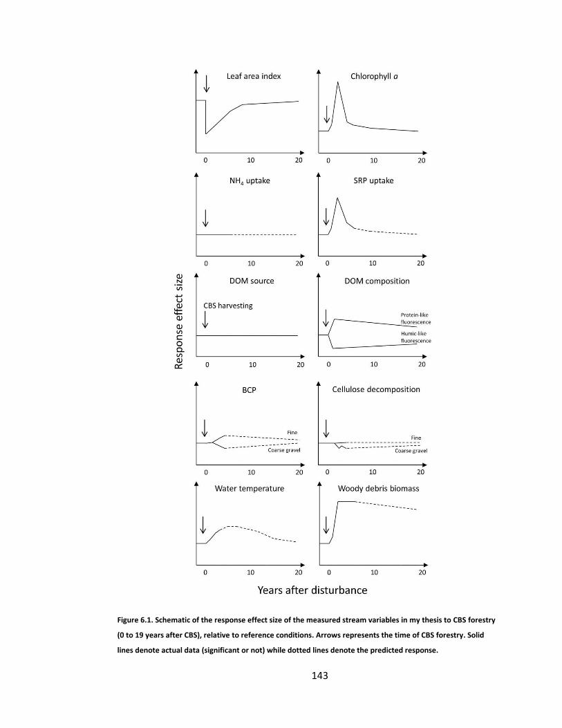
143

Figure 6.1. Schematic of the response effect size of the measured stream variables in my thesis to CBS forestry

(0 to 19 years after CBS), relative to reference conditions. Arrows represents the time of CBS forestry. Solid

lines denote actual data (significant or not) while dotted lines denote the predicted response.

144

Another prominent structural change after CBS forestry was increased

quantities of in-stream woody debris (Chapter 2). This represents a substantial

transfer of OM from the terrestrial compartment of the catchment to the stream

channel. This is consistent with research in headwaters affected by CBS forestry in

northeast Tasmania (Davies et al., 2005) and in similar-sized streams in the Pacific

Northwest of North America (Gomi et al., 2001; Chen et al., 2005; Abdelnour et al.,

2011). Importantly, a significant proportion of this woody debris input into

CBS-affected streams was in contact with the stream, thereby influencing stream

morphology and, potentially, biological functioning (Chapter 2 and 3).

Despite these large physical, structural changes to headwater streams after

CBS forestry, there was no unequivocal change to the chemical composition of

stream water. In particular, there was no apparent change in the main source of

stream DOM after clearfelling (Chapter 4), although there was some change in the

composition of DOM after clearfelling, with a greater relative abundance of protein-

like and a lower relative abundance of humic-like fluorescence in CBS-affected than

in old-growth reaches (Chapter 4). Furthermore, over the 19 years after harvest, the

relative abundance of humic-like fluorescence tended to increase while protein-like

fluorescence tended to decrease; although neither of these trends were statistically

significant (Chapter 4). This suggests that it may take longer than nineteen years for

DOM composition to recover to pre-harvest configurations (Chapter 4), and this is

supported by recent research which found long lasting (up to 50 years after

disturbance) effects of harvesting on stream DOM composition in western North

Carolina (Yamashita et al., 2011).

However, robust conclusions regarding the impact of CBS forestry on DOM

characteristics can only be made once more extensive sampling is undertaken

spanning more than nineteen years after harvesting and across multiple seasons.

Sampling stream water for DOM characteristics should include streams affected by

CBS forestry spanning 80 to 100 years post-harvest because this is the typical

145

rotation period for harvesting in wet eucalypt forest. This would enable forest

managers to determine if certain DOM characteristics, such as humic-like and

protein-like compounds, could return to pre-harvest levels before the next harvest

cycle. Furthermore, because my results indicate that terrestrially derived DOM

controls benthic bacterial activity (Chapter 4), it is critical that we understand if the

contribution of terrestrially derived DOM to headwater streams changes as the

surrounding forest regenerates. An increase in the contribution of terrestrially

derived DOM, for instance, may increase heterotrophic activity, affecting the

aquatic food web and the quantity and lability of DOM transported downstream.

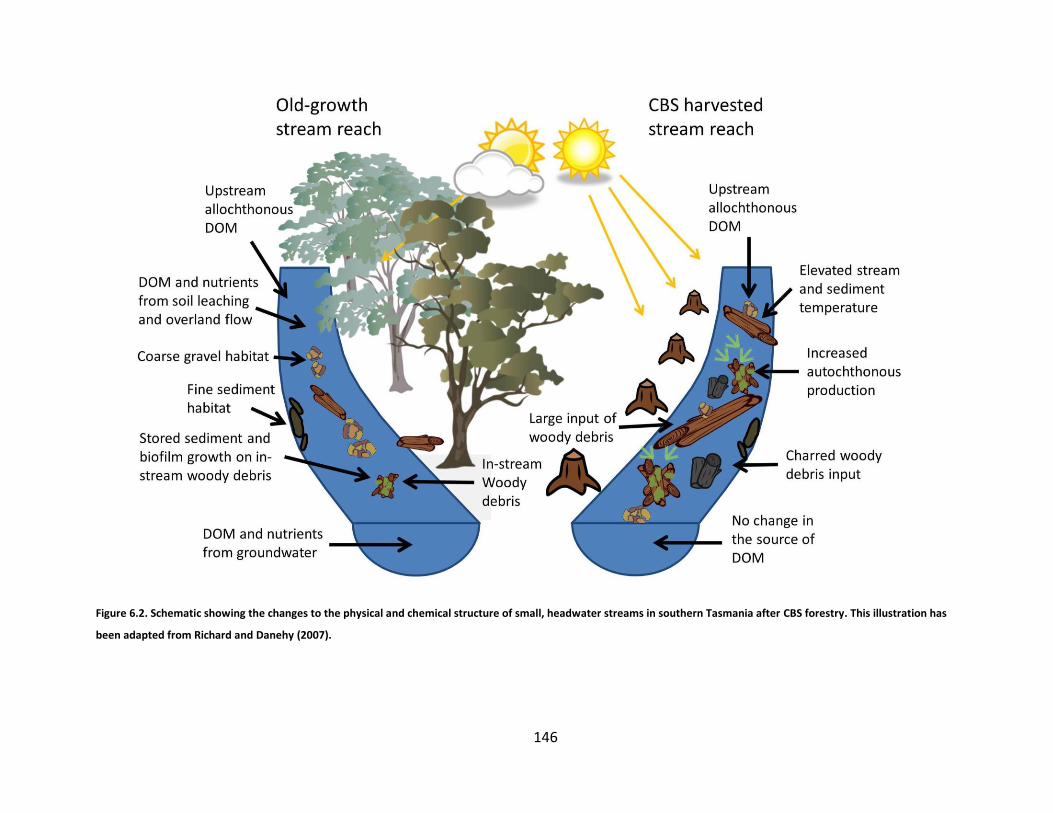
146

Figure 6.2. Schematic showing the changes to the physical and chemical structure of small, headwater streams in southern Tasmania after CBS forestry. This illustration has

been adapted from Richard and Danehy (2007).

147

The large structural changes to headwater streams caused by CBS forestry led

to changes to their functioning (Figure 6.2). My results are consistent with those

from other forested ecosystems where severe riparian disturbance was found to

increase nutrient uptake regardless of whether this disturbance was natural

(Bernhardt et al., 2003) or anthropogenic (Sabater et al., 2000). Additionally, the

pattern of SRP uptake followed that proposed in the nutrient retention succession

model as proposed by Valett et al. (2002). Greater SRP uptake in CBS-affected

reaches was likely due to increased algal and microbial biofilm activity related to the

greater availability of light and surface area of submerged woody debris (Chapter 3).

It is also likely that sorption to charred woody debris and sediment contributed to

the greater SRP uptake in CBS-affected than OG streams (Chapter 3). Burning is

integral to this silvicultural system and contributes much in-stream charcoal.

Therefore, the input of charred woody debris may be a distinctive feature (Figure

6.2), and an important mechanism (Figure 6.3), in regulating uptake and export of P

in these streams. Any changes to silvicultural practices for wet eucalypt forest that

reduces the burning of clearfelled coupes, and presumably the quantity of charred

woody debris in streams, could potentially increase the export of SRP downstream.

Research is needed focusing on SRP sorption to charred woody debris and the role

that this plays in mediating P export. Additionally, research is also required to

determine if SRP flux is actually reduced downstream of CBS coupes because the

effectiveness of a headwater stream’s buffering capacity will depend on whether

the increase in SRP uptake is greater than its flux following CBS forestry operations.

Research can then focus on the potential downstream impacts of any changes in

SRP export. For example, if stream SRP export was significantly reduced in the

immediate years following CBS forestry then this may actually have negative

consequences, such as P deficiencies for downstream ecosystems.

The uptake mechanisms for NH4, and the influence that CBS forestry has upon

them, remains unclear and requires further investigation. Knowledge of the uptake

mechanisms of NH4 is important because, if nitrification was elevated in harvested

148

reaches, this may increase export of N as NO3, because NO3 is a more mobile (i.e.

less bioavailable) form of N than NH4 (Peterson et al., 2001; Bernot and Dodds,

2005).

The decomposition of OM was also affected by the large structural change to

headwater streams after CBS, but the response differed between years and

between benthic habitats (Chapter 5). Generally there was either a reduction or no

change in OM decomposition in the four years after CBS operations, with only BCP

in fine sediment increasing in the third year. The reduction in OM decomposition in

coarse gravel but not fine sediment after CBS was likely a consequence of increased

disturbance (i.e. greater peak flows) to coarse gravel sediment after CBS operations.

This is because physical habitat disturbance has been shown to inhibit development

of bacterial and microbial populations and OM processing on surficial sediments

(Lake, 2000; Atkinson et al., 2008; Entrekin et al., 2008; Gücker et al., 2009;

O'Connor et al., 2012). However, the reasons for the short-term changes in OM

decomposition are uncertain and research is required to determine whether

increased physical habitat disturbance, or other mechanisms, contributes to the

differential response of OM decomposition between habitats. Furthermore, it is not

known whether the short-term changes in OM decomposition have any ecological

consequences for impacted streams and/or downstream ecosystems. For instance,

greater OM decomposition in harvested streams may represent a more rapid

transfer of energy through detrital pathways, as was observed in clearcut

Scandinavian streams (McKie and Malmqvist, 2009), and may increase the export of

more processed, and less labile, organic matter downstream. Research is thus

needed focusing on the ecological consequence of the observed short-term changes

in OM decomposition in both impacted and downstream reaches. If the observed

changes in OM decomposition were found to have ecological consequences, then a

greater understanding of the mechanisms involved will help guide future revisions

to the Forest Practices Code (2000) in order to minimise changes to benthic OM

decomposition in headwater streams and downstream ecosystems.

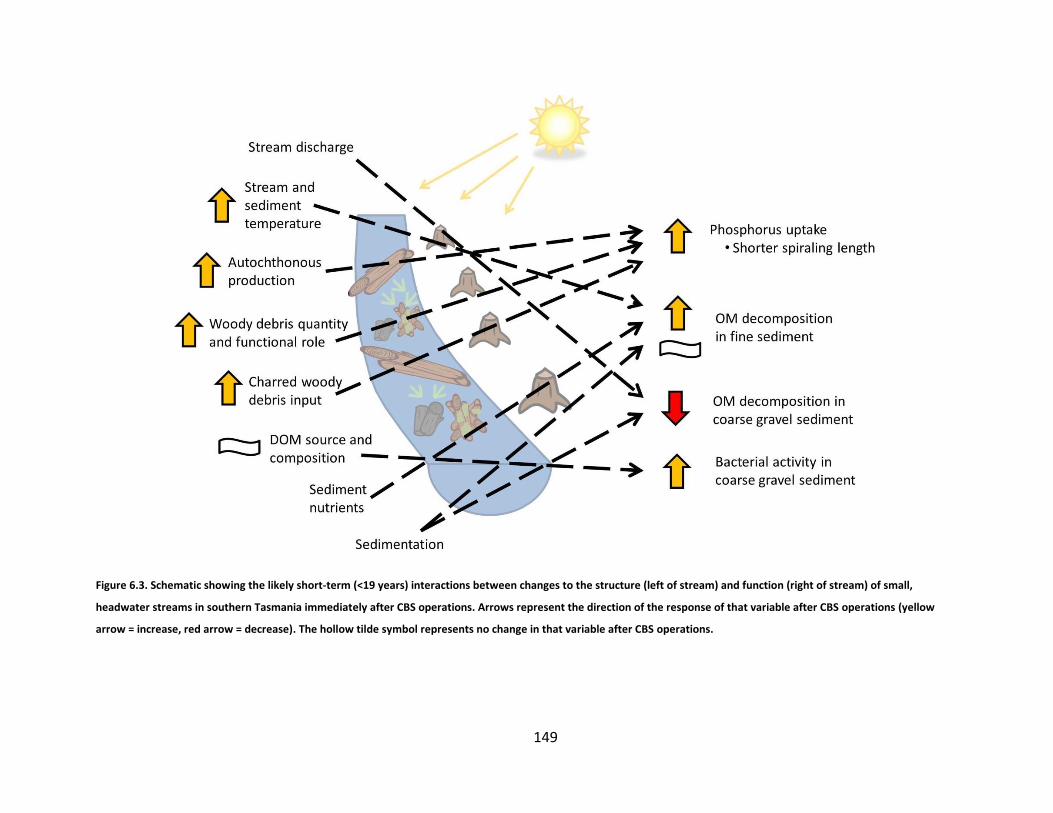
149

Figure 6.3. Schematic showing the likely short-term (<19 years) interactions between changes to the structure (left of stream) and function (right of stream) of small,

headwater streams in southern Tasmania immediately after CBS operations. Arrows represent the direction of the response of that variable after CBS operations (yellow

arrow = increase, red arrow = decrease). The hollow tilde symbol represents no change in that variable after CBS operations.

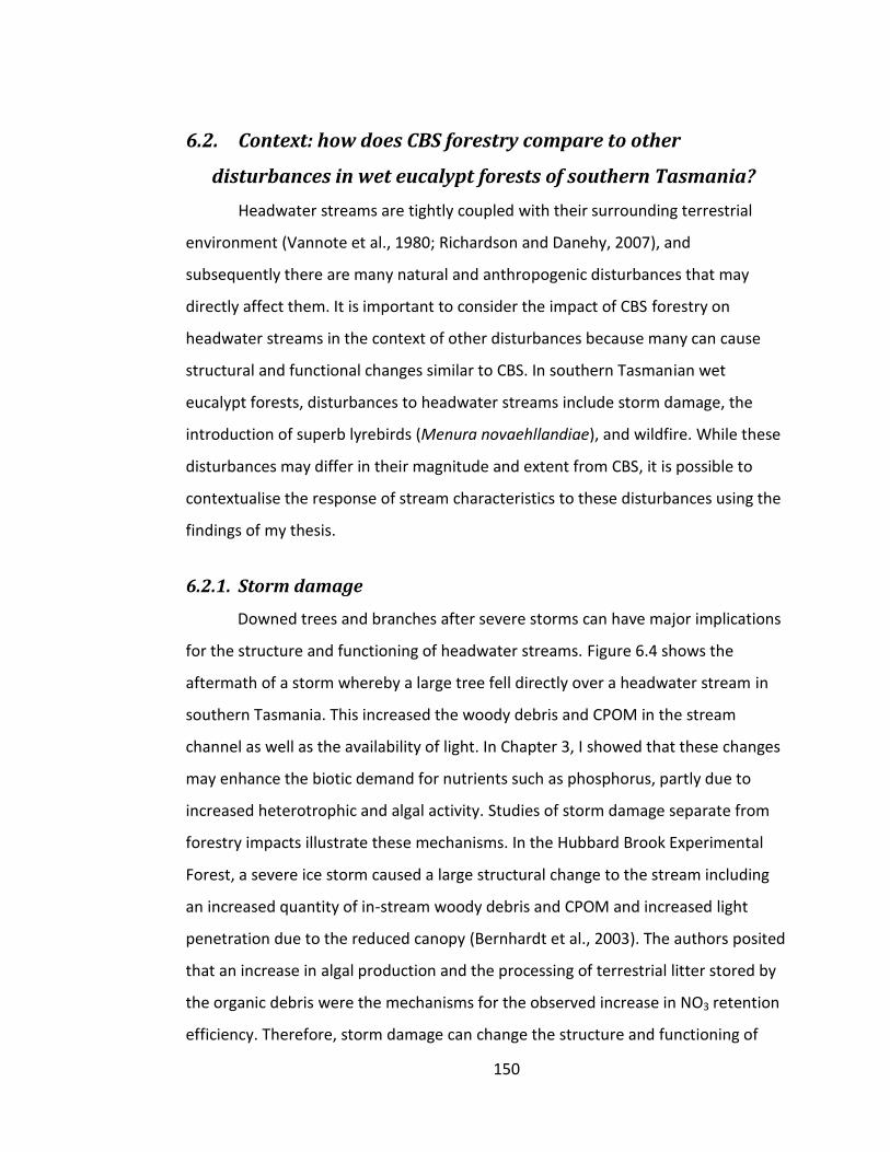
150

6.2. Context: how does CBS forestry compare to other

disturbances in wet eucalypt forests of southern Tasmania?

Headwater streams are tightly coupled with their surrounding terrestrial

environment (Vannote et al., 1980; Richardson and Danehy, 2007), and

subsequently there are many natural and anthropogenic disturbances that may

directly affect them. It is important to consider the impact of CBS forestry on

headwater streams in the context of other disturbances because many can cause

structural and functional changes similar to CBS. In southern Tasmanian wet

eucalypt forests, disturbances to headwater streams include storm damage, the

introduction of superb lyrebirds (Menura novaehllandiae), and wildfire. While these

disturbances may differ in their magnitude and extent from CBS, it is possible to

contextualise the response of stream characteristics to these disturbances using the

findings of my thesis.

6.2.1. Storm damage

Downed trees and branches after severe storms can have major implications

for the structure and functioning of headwater streams. Figure 6.4 shows the

aftermath of a storm whereby a large tree fell directly over a headwater stream in

southern Tasmania. This increased the woody debris and CPOM in the stream

channel as well as the availability of light. In Chapter 3, I showed that these changes

may enhance the biotic demand for nutrients such as phosphorus, partly due to

increased heterotrophic and algal activity. Studies of storm damage separate from

forestry impacts illustrate these mechanisms. In the Hubbard Brook Experimental

Forest, a severe ice storm caused a large structural change to the stream including

an increased quantity of in-stream woody debris and CPOM and increased light

penetration due to the reduced canopy (Bernhardt et al., 2003). The authors posited

that an increase in algal production and the processing of terrestrial litter stored by

the organic debris were the mechanisms for the observed increase in NO3 retention

efficiency. Therefore, storm damage can change the structure and functioning of

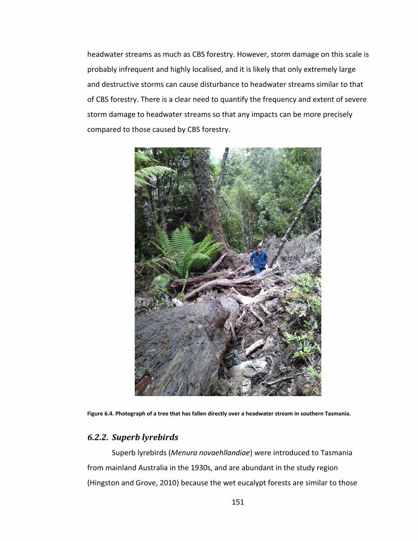
151

headwater streams as much as CBS forestry. However, storm damage on this scale is

probably infrequent and highly localised, and it is likely that only extremely large

and destructive storms can cause disturbance to headwater streams similar to that

of CBS forestry. There is a clear need to quantify the frequency and extent of severe

storm damage to headwater streams so that any impacts can be more precisely

compared to those caused by CBS forestry.

Figure 6.4. Photograph of a tree that has fallen directly over a headwater stream in southern Tasmania.

6.2.2. Superb lyrebirds

Superb lyrebirds (Menura novaehllandiae) were introduced to Tasmania

from mainland Australia in the 1930s, and are abundant in the study region

(Hingston and Grove, 2010) because the wet eucalypt forests are similar to those

152

where they occur naturally (Ashton and Bassett, 1997). Superb lyrebirds feed mainly

on terrestrial invertebrates and seeds that they find by scratching through the leaf

litter (Ashton and Bassett, 1997). The process of scratching in search of food can

impact headwater streams by disturbing OM and surface soil close to or even in the

stream channel (Figure 6.5). Although the frequency and extent of their disturbance

in headwater stream beds remains unquantified, lyrebirds are capable of

considerable activity: Ashton and Bassett (1997) found that in a single year they can

displace 188.5 t ha-1 of soil and 80.5 t ha-1 of leaf litter.

When lyrebirds scratch up the soil and litter near the stream channel they

are providing a source of fresh soil organic material that can easily be transported

into the stream via overland flow during storm events, which will have at least three

major implications. First, this fresh soil organic material will likely be highly

bioavailable, because it has undergone minimal microbial processing (Likens et al.,

1970; Fellman et al., 2009), and may increase the activity of benthic bacteria (as was

seen in Chapter 5). Second, the soil and CPOM that lyrebirds transfer into the

stream may accumulate behind debris dams and become an additional source of

energy for fungi, heterotrophic bacteria and invertebrates. A third implication is that

future investigators of these streams need to be aware of lyrebird disturbances

within headwater streams because it would be easy to inadvertently confound

lyrebird effects with those attributed to CBS activities, by, for example, accidentally

co-locating sampling patches with those disturbed by lyrebirds (Figure 6.5).

Overall, lyrebird damage to the stream channel may increase the activity of

stream heterotrophic bacteria which could lead to a greater processing of OM and

even a more rapid transfer of energy and nutrients in headwaters affected by

lyrebirds (McKie and Malmqvist, 2009). However, unlike other stream disturbances

(i.e. harvesting, wildfire and storm damage), lyrebirds will not cause large episodic,

physical changes to stream and forest structure. Instead the damage will likely be

patchy and continuous throughout the year. Future research should quantify how

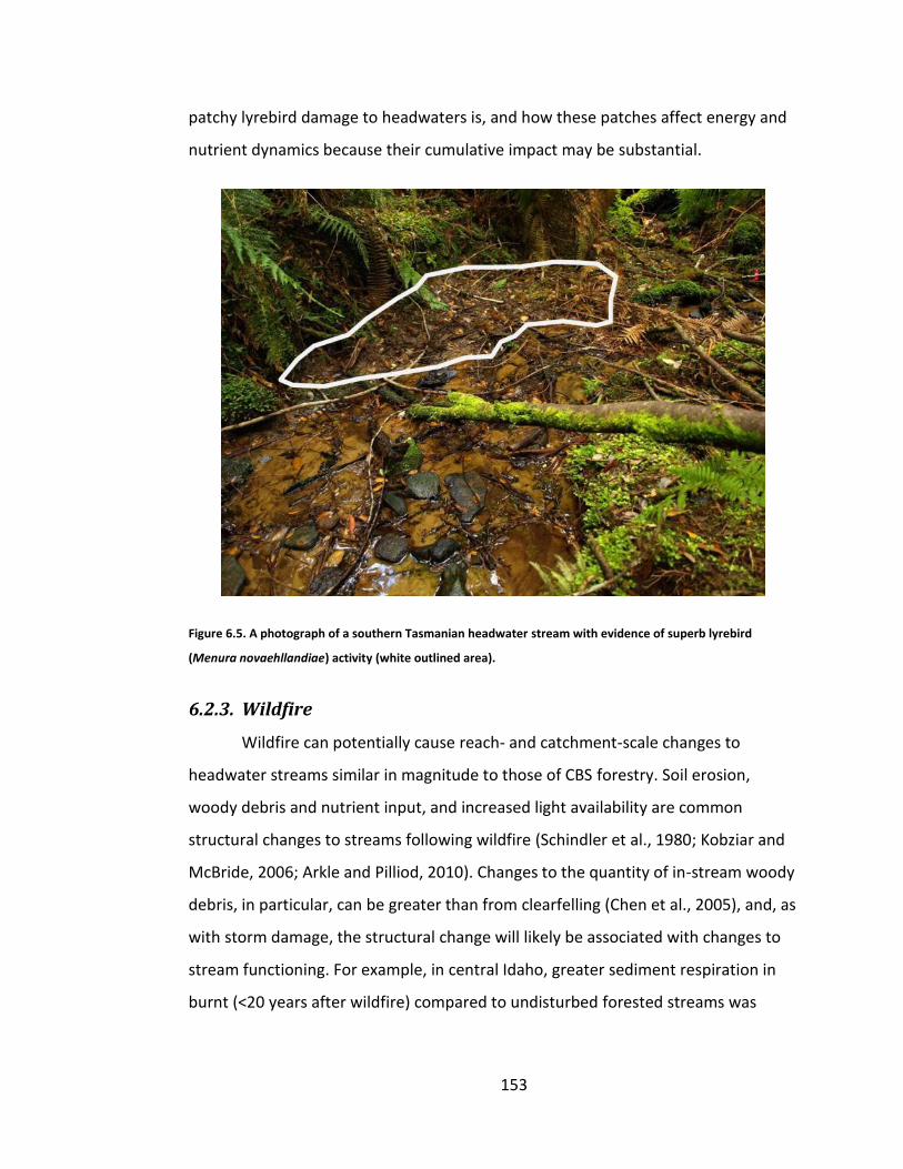
153

patchy lyrebird damage to headwaters is, and how these patches affect energy and

nutrient dynamics because their cumulative impact may be substantial.

Figure 6.5. A photograph of a southern Tasmanian headwater stream with evidence of superb lyrebird

(Menura novaehllandiae) activity (white outlined area).

6.2.3. Wildfire

Wildfire can potentially cause reach- and catchment-scale changes to

headwater streams similar in magnitude to those of CBS forestry. Soil erosion,

woody debris and nutrient input, and increased light availability are common

structural changes to streams following wildfire (Schindler et al., 1980; Kobziar and

McBride, 2006; Arkle and Pilliod, 2010). Changes to the quantity of in-stream woody

debris, in particular, can be greater than from clearfelling (Chen et al., 2005), and, as

with storm damage, the structural change will likely be associated with changes to

stream functioning. For example, in central Idaho, greater sediment respiration in

burnt (<20 years after wildfire) compared to undisturbed forested streams was

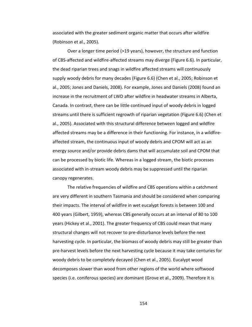
154

associated with the greater sediment organic matter that occurs after wildfire

(Robinson et al., 2005).

Over a longer time period (>19 years), however, the structure and function

of CBS-affected and wildfire-affected streams may diverge (Figure 6.6). In particular,

the dead riparian trees and snags in wildfire affected streams will continuously

supply woody debris for many decades (Figure 6.6) (Chen et al., 2005; Robinson et

al., 2005; Jones and Daniels, 2008). For example, Jones and Daniels (2008) found an

increase in the recruitment of LWD after wildfire in headwater streams in Alberta,

Canada. In contrast, there can be little continued input of woody debris in logged

streams until there is sufficient regrowth of riparian vegetation (Figure 6.6) (Chen et

al., 2005). Associated with this structural difference between logged and wildfire

affected streams may be a difference in their functioning. For instance, in a wildfire-

affected stream, the continuous input of woody debris and CPOM will act as an

energy source and/or provide debris dams that will accumulate soil and CPOM that

can be processed by biotic life. Whereas in a logged stream, the biotic processes

associated with in-stream woody debris may be suppressed until the riparian

canopy regenerates.

The relative frequencies of wildfire and CBS operations within a catchment

are very different in southern Tasmania and should be considered when comparing

their impacts. The interval of wildfire in wet eucalypt forests is between 100 and

400 years (Gilbert, 1959), whereas CBS generally occurs at an interval of 80 to 100

years (Hickey et al., 2001). The greater frequency of CBS could mean that many

structural changes will not recover to pre-disturbance levels before the next

harvesting cycle. In particular, the biomass of woody debris may still be greater than

pre-harvest levels before the next harvesting cycle because it may take centuries for

woody debris to be completely decayed (Chen et al., 2005). Eucalypt wood

decomposes slower than wood from other regions of the world where softwood

species (i.e. coniferous species) are dominant (Grove et al., 2009). Therefore it is

155

possible that over many harvesting cycles there could be a vastly greater biomass of

woody debris in CBS-affected than wildfire-affected streams.

Figure 6.6. A conceptual diagram showing the difference in the frequency of woody debris input between

headwater streams affected by wildfire (a) and (b) harvesting.

6.3. Paradigms for assessing disturbance

The broad aim of this thesis was to assess the short-term structural and

functional changes to headwater streams caused by CBS forestry. The chapters are

shaped around the most important ecological theories and concepts relevant to my

research. In particular, my work provides a contribution to experimental design for

impact assessment and theories of ecological resistance, resilience (Holling, 1973;

Lake and Barmuta, 1986; Power, 1999) and ecological integrity impacts (Downes et

al., 2002; Schallenberg et al., 2011). Additionally, concepts, such as the River

Continuum Concept (Chapter 1 and 6), upstream heterogeneous zone (UHZ; Chapter

156

1), the nutrient retention succession model (Chapter 3), and landscape ecology

(Chapters 4 and 5), were integral in the design and development of the thesis

experiments and also in the discussion of management implications to do with CBS

forestry.

6.3.1. Resistance and resilience of individual stream variables to CBS

forestry

The resistance (ability to resist or remain unchanged after disturbance) and

resilience (ability to recover or return to its pre-disturbance state) of individual

stream variables to CBS forestry is important to understand because it describes the

response of headwater to harvesting (see Chapter 1). The majority of the structural

and functional components measured in southern Tasmanian headwater streams

showed no resistance or resilience to CBS in the short-term (1 to 19 years after

operations) (Table 6.1). The lack of resistance of many stream variables is not

surprising given the large physical change that CBS represents and as documented

frequently in other studies of clearfell harvesting (Johnson and Jones, 2000; Gomi et

al., 2001; Swank et al., 2001; Chen et al., 2005; Moore et al., 2005; Clapcott, 2007;

Kreutzweiser et al., 2008; Gravelle et al., 2009; McKie and Malmqvist, 2009; Clapcott

and Barmuta, 2010; Watson and Barmuta, 2010).

Nevertheless, one structural and two functional components did show

evidence for resistance after CBS forestry (Table 6.1). The source of DOM did not

appear to be affected by CBS operations (Chapter 5). Similarly, the spiralling length

of NH4 and the cellulose decomposition of fine sediment were also not affected by

CBS (Chapters 3 and 4, respectively). However, the apparent resistance of DOM

source to CBS was likely due to the relatively small proportion of the stream channel

that is impact by harvesting operations. An increase in the intensity and extent of

CBS operations (i.e. greater proportion of the catchment harvested) may therefore

cause a change to the source of DOM by increasing the contribution of

autochthonous DOM production.

157

For the other variables measured, the resilience to CBS forestry was difficult

to assess because the oldest coupes harvested under the current prescriptions were

only 19 years old. Nevertheless, there was evidence for short-term resilience of algal

activity (as chlorophyll a) and SRP nutrient spiralling. Chlorophyll a initially increased

after harvesting but appeared to decline, recovering to near old-growth levels six

years after clearfelling (Figure 6.1). Correspondingly, the SRP uptake velocity in the

CBS-affected streams approached that of OG streams seven years after clearfelling

(Figure 3.4; Chapter 3), indicating that algal uptake is likely an important mechanism

for SRP uptake in these streams. This decline in SRP nutrient spiralling after seven

years is similar to that proposed by Valett et al. (2002) who suggested that after five

years nutrient retention would decline rapidly due to a decrease in primary and

heterotrophic in-stream production associated the depletion of stream organic

matter and/or light availability as the surrounding riparian vegetation regrows.

The resilience of stream responses is probably of most interest to forest

managers given that it is difficult to prevent changes (i.e. loss of resistance) to many

stream components after clearfelling. To gain a better understanding of resilience

after CBS forestry, many of the structural and functional measures will need to be

assessed over a much longer time period than was assessed in this thesis. This is

because many of the structural changes caused by CBS forestry may take decades to

return to a pre-disturbance state. For example, woody debris deposited after

disturbance can decay very slowly (Chen et al., 2005) and continue influencing the

stream for over six decades (Wallace et al., 1991; Gomi et al., 2001). Furthermore,

changes in DOM composition can linger for up to 50 years after forest harvesting

due to continued changes in soil OM characteristics and OM inputs (Yamashita et

al., 2011). Given that many of the functional changes observed in this study were

related to the large structural changes, it may be expected that the recovery of the

functional variables will follow that of the structural ones. Clearly, a longer time

span of survey-based research is needed (>19 years after harvesting) which would

be strengthened by the inclusion of a long-term MBACI study. Space-for-time

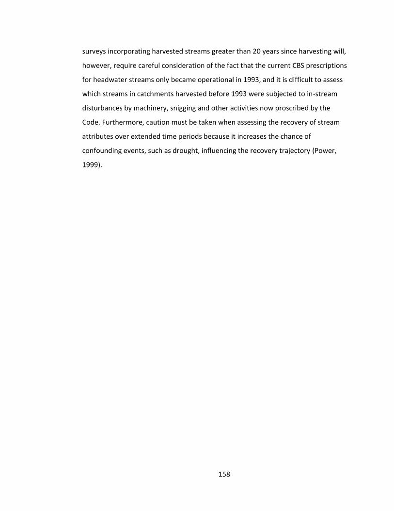
158

surveys incorporating harvested streams greater than 20 years since harvesting will,

however, require careful consideration of the fact that the current CBS prescriptions

for headwater streams only became operational in 1993, and it is difficult to assess

which streams in catchments harvested before 1993 were subjected to in-stream

disturbances by machinery, snigging and other activities now proscribed by the

Code. Furthermore, caution must be taken when assessing the recovery of stream

attributes over extended time periods because it increases the chance of

confounding events, such as drought, influencing the recovery trajectory (Power,

1999).

159

Table 6.1. Summary of the evidence for resistance and resilience of the structural and functional attributes of headwater streams after CBS operations (<19 years after

harvest).

Evidence for resistance? Evidence for resilience?

Structural measures

Quantity of woody

debris

No Greater woody debris in harvested streams. No However, only surveyed 2 and 7 years after harvesting.

DOM source Yes No change in the source of DOM between harvested and old-

growth streams or along gradient of years since harvest.

NA NA.

DOM composition Ambiguous Differences in composition between harvested and old-

growth streams but no relationship with years since harvest.

Maybe Evidence for a longer-term (>19 years) recovery after

harvesting.

Chlorophyll a No Greater chlorophyll a in the immediate years after harvesting. Yes Yes. Return near old-growth values after 6 years.

Functional measures

SRP uptake No Greater SRP uptake after harvesting. Yes SRP uptake in harvested streams approaches that of OG after

7 years.

NH4 uptake Yes No change in NH4 uptake after harvesting. However, uptake

mechanisms are not yet understood.

NA NA.

BCP Ambiguous Resistance only for first year after harvesting in coarse gravel

and fine sediment habitat. Increasing or decreasing

thereafter.

No However, only surveyed four years after harvesting.

Cellulose

decomposition.

Ambiguous Resistance every year after harvesting in fine sediment

habitat. But decrease after first years in coarse gravel habitat.

No However, only surveyed four years after harvesting.

160

6.3.2. Stream ecological integrity

The measurement of various structural and functional components of

headwater streams and their response to CBS forestry allowed me to make

informed assessments regarding changes to the ecological integrity of headwater

streams. This is because ecological integrity is assessed as the maintenance of the

structure and function of an ecosystem similar to reference condition reflecting

minimal anthropogenic impacts (Meyer, 1997; Schallenberg et al., 2011). Based on

this definition, it can be concluded that CBS forestry altered the ecological integrity

of headwater streams in the short-term (1 to 19 years after harvesting) because

there were changes to the structure and function that were significantly different

from reference streams.

However, it is important to recognise that conclusions drawn using this

definition depends on the approach used to classify the reference condition, and

more specifically whether the reference condition accounts for natural variability

within an ecosystem. Natural ecosystems do not maintain a static state but rather

their structural and functional components vary in response to environmental

conditions (e.g. climate, wildfire, and species lifecycles). For instance, as mentioned

in Section 6.2.3, wildfire can cause changes to stream ecosystems to the same

extent as clearfelling and, without including this natural variability in the description

of a reference condition, we lack context to judge the severity of anthropogenic

disturbance upon an ecosystem. Therefore, future research assessing the resistance,

resilience, and ecological integrity of headwater streams must not take a static view

of the ecosystems, but characterise the natural variability that may occur over time

and incorporate this into assessments of anthropogenic disturbance.

6.4. Management implications

Altering prescriptions for riparian buffers and dispersing CBS operations in

space and time were suggested in Chapter 5 to be the main management actions

available for forest managers to reduce the impact of CBS forestry on headwater

161

streams. Riparian buffers mitigate changes to the stream environment after forest

harvesting (Davies and Nelson, 1994; Zwieniecki and Newton, 1999; Thompson et

al., 2009), but they were considered impractical because the high frequency of

headwater streams flowing through CBS coupes would leave little remaining forest

to harvest. Furthermore, reducing the burning of the MEZ to retain some living

vegetation may also not be feasible because it is difficult to control a fire of the

intensity needed for eucalypt regeneration. Despite their impracticality, riparian

buffers or reducing the burning of the MEZ would be the actions most likely to

reduce the impact of CBS forestry at the reach-scale.

The problems with implementing effective riparian protection (buffer strips

or reducing the burning of the MEZ) means that dispersing CBS operations in space

and time may be the only feasible management option available for forest

managers. The dispersal of CBS coupes in space and time is currently employed in

Tasmania to mitigate downstream impacts through dilution from inflowing tributary

streams (Forest Practices Board, 2000). However, it is not yet known if this strategy

is effective in mitigating downstream ecological impacts associated with forest

operations (i.e. elevated downstream water temperature). An understanding of how

the dispersal of CBS coupes in space and time affects downstream ecosystems is

critical because intensification of CBS operations in the landscape could amplify

downstream impacts. For instance, Chapter 4 showed that the source of DOM was

not influenced by harvesting operations. It was suggested that the contribution of

DOM from the entire catchment was much greater than that of the CBS-affected

reach because only a small proportion of the stream channel is usually affected by

CBS operations. However, if there was an increase in the intensity or extent of CBS

operations in the landscape, then we may begin to detect changes to the source of

DOM that reflects a more intensively harvested catchment (i.e. more

autochthonous DOM production). Careful planning of the intensity and extent of

CBS coupes in the landscape will ensure that localised, reach-scale impacts will not

adversely impact downstream ecosystems.

162

One important finding of my research was that some of the structural

changes to headwaters that occur under current forest practices may actually be

beneficial in reducing some negative effects for downstream ecosystems.

Consequently, forest managers could manipulate these mechanisms to reduce

downstream impacts. For example, the greater woody debris input and light

available after harvesting operations may reduce excess SRP export to downstream

ecosystems by increasing SRP uptake and retention (Chapter 3). Elsewhere,

enhanced NO3 retention was found in a headwater stream after a severe ice storm

that increased woody debris, light penetration, and presumably biotic uptake

(Bernhardt et al., 2003). Without the increase in NO3 retention, the export of NO3

would have been 80 to 140% higher (Bernhardt et al., 2003). In this instance, a

combination of 1) reducing the potential for excess nutrient input via the retention

of riparian vegetation and 2) increasing stream nutrient demand via greater light

availability and woody debris input, may benefit both headwaters (reduced excess

nutrient input) and downstream ecosystems (reduced excess nutrient export).

6.5. Future directions

The findings in this thesis of the response of headwater streams to CBS

forestry are unique to small, headwater streams flowing through wet eucalypt

forest in predominately doleritic catchments of southern Tasmania. While a small

number of the potential structural and functional aspects of headwater streams

were examined in this thesis, there are many more which, if assessed, could

contribute to the understanding of the impact of CBS forestry on headwater stream

ecosystems and their recovery. Importantly, the community structure of these

small, headwater streams has not yet been examined, and this should be the

immediate focus of future research. Aquatic macroinvertebrates play a critical role

in forested, headwater streams because they process CPOM into fine particulate

organic matter (FPOM) which becomes available as a food source for other aquatic

organisms and can be more easily exported downstream (Wipfli et al., 2007).

163

Furthermore, the longitudinal movement of macroinvertebrates from headwater

streams can be an important food source for downstream vertebrates such as fish

(Ormerod et al., 2004; Romaniszyn et al., 2007). Consequently, macroinvertebrates

link terrestrial OM input with the productivity of upstream and downstream aquatic

and riparian food webs. I recommend that research should focus on 1) the

abundance and diversity of aquatic macroinvertebrates in small, headwater streams

flowing through wet eucalypt forest, 2) the impact that CBS forestry has upon their

abundance and diversity, and 3) quantifying the downstream dispersal of aquatic

macroinvertebrates. Understanding the role of aquatic invertebrates in headwater

streams flowing through wet eucalypt forest and the impact of CBS forestry will

allow forest practices to be designed that maximise their diversity and functional

role.

Of the structural and functional attributes of headwater streams that were

assessed in this study, many require continued research. First, more research is

needed focusing on the uptake mechanisms of NH4. Although this study identified

that the large structural change to CBS-affected stream reaches increased SRP

uptake, the uptake of NH4 was not affected and the uptake mechanisms for NH4

remain unknown (Chapter 3). It was suggested that rapid nitrification of NH4 in the

CBS-affected streams may be masking its detection during the nutrient addition

experiments (Chapter 3). If nitrification was high within the CBS forestry streams,

this may increase the export of N as NO3 to downstream ecosystems. Therefore, it is

a high priority to quantify rates of nitrification, its drivers, and also its reach-scale

impact on NH4 uptake in benthic sediment of undisturbed and CBS-affected

streams. Second, research is needed to assess the spatial distribution and temporal

variation of benthic habitats and the impact of CBS forestry because habitats may

respond differently to CBS operations (Chapter 5). Moreover, it is important to

determine if streams show the same pattern of response (i.e. rates of OM

decomposition) at the reach-scale to ensure that the observed response of OM

decomposition in habitats are not scale-dependent.

164

Continued research is needed focusing on the trajectories and recovery

times of stream variables after CBS forestry, because many of the structural and

functional characteristics of headwater streams showed no resilience to CBS

forestry in the short-term (<19 years after harvesting) (Table 6.1). As previously

mentioned, however, any results from space for time research incorporating CBS

impacted streams greater than 19 years since harvesting will require careful

interpretation because the current CBS prescriptions for headwater streams only

became operational in 1993. Research is also required on the adequate dispersal of

CBS operations in space and time to ensure that headwaters are managed to

minimise impacts on downstream ecosystems.

It is imperative that any future research incorporates how changes in

ecosystem structure and functioning that are caused by CBS forestry compares with

natural disturbances such as wildfire or storm damage. Assessing the response of

headwaters due to CBS forestry in the context of this natural variability will allow

quantification of the degree of change from that which occurs naturally. This

information could allow wet eucalypt forests and headwater streams to be

managed in a way that follows the emulation of natural disturbance (END)

paradigm. In the context of streams, END aims to harvest forested catchments in a

way that results in its structural and functional features, and their temporal and

spatial patterns, resembling what would occur due to natural disturbance

(Kreutzweiser et al., 2012; Sibley et al., 2012). However, adopting this harvesting

approach would likely reduce the role of CBS in wet eucalypt forests, primarily

because wildfire, which is the main natural process that CBS forestry emulates,

occurs over much longer time intervals (100 to 400 years; Gillbert, 1959) than CBS

forestry (80 to 100 years; Hickey et al., 2001).

165

Chapter 7. References

ABDELNOUR, A., STIEGLITZ, M., PAN, F. & MCKANE, R. 2011. Catchment hydrological responses to forest harvest amount and spatial pattern. Water Resources Research, 47.

ALEXANDER, R. B., BOYER, E. W., SMITH, R. A., SCHWARZ, G. E. & MOORE, R. B. 2007. The role of headwater streams in downstream water quality. Journal of the American Water Resources Association, 43, 41-59.

AMON, R. M. W. & BENNER, R. 1996. Bacterial utilization of different size classes of dissolved organic matter. Limnology and Oceanography, 41, 41-51.

ANDERSON, M. J. 2001. A new method for non-parametric multivariate analysis of variance. Austral Ecology, 26, 32-46.

APHA 2005. Standard Methods for the Examination of Water and Wastewater, Washington, DC., American Public Health Association.

ARKLE, R. S. & PILLIOD, D. S. 2010. Prescribed fires as ecological surrogates for wildfires: A stream and riparian perspective. Forest Ecology and Management, 259, 893-903.

ASHTON, D. 1975. Studies of litter in Eucalyptus regnans forests. Australian Journal of Botany, 23, 413-433.

ASHTON, D. H. & BASSETT, O. D. 1997. The effects of foraging by the superb lyrebird (Menura novae-hollandiae) in Eucalyptus regnans forests at Beenak, Victoria. Austral Ecology, 22, 383-394.

ATKINSON, B. L., GRACE, M. R., HART, B. T. & VANDERKRUK, K. E. N. 2008. Sediment instability affects the rate and location of primary production and respiration in a sand-bed stream. Journal of the North American Benthological Society, 27, 581-592.

AUMEN, N. G., HAWKINS, C. P. & GREGORY, S. V. 1990. Influence of woody debris on nutrient retention in catastrophically disturbed streams. Hydrobiologia, 190, 183-192.

BAILLIE, B. R., GARRETT, L. G. & EVANSON, A. W. 2008. Spatial distribution and influence of large woody debris in an old-growth forest river system, New Zealand. Forest Ecology and Management, 256, 20-27.

BATES, D. M., MAECHLER, M. & BOLKER, B. 2011. lme4: Linear mixed-effects models using S4 classes. CRAN.

BENDA, L., POFF, N. L., MILLER, D., DUNNE, T., REEVES, G., PESS, G. & POLLOCK, M. 2004. The network dynamics hypothesis: How channel networks structure riverine habitats. BioScience, 54, 413-427.

BENFIELD, E. F., WEBSTER, J. R., TANK, J. L. & HUTCHENS, J. J. 2001. Long-term patterns in leaf breakdown in streams in response to watershed logging. International Review of Hydrobiology, 86, 467-474.

BENJAMINI, Y. & HOCHBERG, Y. 2000. On the adaptive control of the false discovery rate in multiple testing with independent statistics. Journal of Educational and Behavioral Statistics, 25, 60-83.

BENSTEAD, J. P. & HURYN, A. D. 2011. Extreme seasonality of litter breakdown in an arctic spring-fed stream is driven by shredder phenology, not temperature. Freshwater Biology, 56, 2034-2044.

BERG, N., CARLSON, A. & AZUMA, D. 1998. Function and dynamics of woody debris in stream reaches in the central Sierra Nevada, California. Canadian Journal of Fisheries and Aquatic Sciences, 55, 1807-1820.

166

BERGFUR, J., JOHNSON, R. K., SANDIN, L. & GOEDKOOP, W. 2007. Assessing the ecological integrity of boreal streams: A comparison of functional and structural responses. Fundamental and Applied Limnology, 168, 113-125.

BERGGREN, M., LAUDON, H. & JANSSON, M. 2009. Aging of allochthonous organic carbon regulates bacterial production in unproductive boreal lakes. Limnology and Oceanography, 54, 1333-1342.

BERNHARDT, E. S., HALL JR, R. O. & LIKENS, G. E. 2002. Whole-system estimates of nitrification and nitrate uptake in streams of the Hubbard Brook Experimental Forest. Ecosystems, 5, 419-430.

BERNHARDT, E. S., LIKENS, G. E., BUSO, D. C. & DRISCOLL, C. T. 2003. In-stream uptake dampens effects of major forest disturbance on watershed nitrogen export. Proceedings of the National Academy of Sciences of the United States of America, 100, 10304-10308.

BERNOT, M. J. & DODDS, W. K. 2005. Nitrogen retention, removal, and saturation in lotic ecosystems. Ecosystems, 8, 442-453.

BERTILSSON, S. & JONES, J. N. 2003. Supply of Dissolved Organic Matter to Aquatic Ecosystems: Autochthonous Sources. In: FINDLAY, S. E. G. & SINSABAUGH, R. L. (eds.) Aquatic Ecosystems: Interactivity of Dissolved Organic Matter. USA: Academic Press.

BESCHTA, R. L. & TAYLOR, R. L. 1988. Stream temperature increases and land use in a forested Oregon watershed. Water Resources Bulletin, 24, 19-25.

BIGGS, B. J. F. & KILROY, C. 2000. Stream Periphyton Monitoring Manual. Christchurch, New Zealand: NIWA for The New Zealand Ministry for the Environment.

BILBY, R. E. & BISSON, P. A. 1998. Function and Distribution of Large Woody Debris. In: NAIMAN, R. J. & BILBY, R. E. (eds.) River Ecology and Management - Lessons from the Pacific Coastal Ecoregion. New York: Springer-Verlag.

BILBY, R. E. & LIKENS, G. E. 1980. Importance of Organic Debris Dams in the Structure and Function of Stream Ecosystems. Ecology, 61, 1107-1113.

BILBY, R. E. & WARD, J. W. 1989. Changes in Characteristics and Function of Woody Debris with Increasing Size of Streams in Western Washington. Transactions of the American Fisheries Society, 118, 368-378.

BILBY, R. E. & WARD, J. W. 1991. Characteristics and function of large woody debris in streams draining old-growth, clear-cut, and second-growth forests in southwestern Washington. Canadian Journal of Fisheries and Aquatic Sciences, 48, 2499-2508.

BIRD, D. F. & KALFF, J. 1984. Empirical relationships between bacterial abundance and chlorophyll concentration in fresh and marine waters. Canadian Journal of Fisheries and Aquatic Sciences, 41, 1015-1023.

BISSON, P. A., BILBY, R. E., BRYANT, M. D., DOLLOFF, C. A., GRETTE, G. B., HOUSE, R. A., MURPHY, M. L., KOSKI, K. V. & SEDELL, J. R. 1987. Large woody debris in forested streams in the Pacific Northwest: Past, present, and future. In: SALO, E. O. & CUNDY, T. W. (eds.) Streamside management: forestry and fishery interactions. Seattle: University of Washington Press.

BLOTT, S. J. & PYE, K. 2001. Gradistat: a grain size distribution and statistics package for the analysis of unconsolidated sediments. Earth Surface Processes and Landforms, 26, 1237-1248.

BOND, N. R., SABATER, S., GLAISTER, A., ROBERTS, S. & VANDERKRUK, K. 2006. Colonisation of introduced timber by algae and invertebrates, and its potential role in aquatic ecosystem restoration. Hydrobiologia, 556, 303-316.

167

BOULTON, A. J. & QUINN, J. M. 2000. A simple and versatile technique for assessing cellulose decomposition potential in floodplain and riverine sediments. Archiv fur Hydrobiologie, 150, 133-151.

BRUDER, A., CHAUVET, E. & GESSNER, M. O. 2011. Litter diversity, fungal decomposers and litter decomposition under simulated stream intermittency. Functional Ecology, 25, 1269-1277.

BRYANT, M. D., GOMI, T. & PICCOLO, J. J. 2007. Structures linking physical and biological processes in headwater streams of the Maybeso Watershed, southeast Alaska. Forest Science, 53, 371-383.

BUESING, N. & GESSNER, M. O. 2003a. Incorporation of radiolabeled leucine into protein to estimate bacterial production in plant litter, sediment, epiphytic biofilms, and water samples. Microbial Ecology, 45, 291-301.

BUESING, N. & GESSNER, M. O. 2003b. Incorporation of radiolabelled leucine into protein to estimate bacterial production in plant litter, sediment, epiphytic biofilms, and water samples. Microbial Ecology, 45, 291-301.

BUNN, S. E. 1988. Processing of leaf litter in two northern jarrah forest streams, Western Australia: II. The role of macroinvertebrates and the influence of soluble polyphenols and inorganic sediment. Hydrobiologia, 162, 211-223.

BUREAU OF METEOROLOGY. 2012. Tasmanian annual climate summary archive [Online]. Australian Government. Available: http://www.bom.gov.au/climate/current/annual/tas/archive/ [Accessed January 2012 January 2012].

BURNHAM, K. P. & ANDERSON, D. R. 2002. Model selection and multimodel inference: a practical information-theoretic approach, New York, Springer.

BUTTURINI, A. & SABATER, F. 1998. Ammonium and phosphate retention in a Mediterranean stream: hydrological versus temperature control. Canadian Journal of Fisheries and Aquatic Sciences, 55, 1938-1945.

CFEV DATABASE V1.0 2005. Conservation of freshwater ecosystem values project, Water Resources Division, Department of Primary Industries and Water. Tasmania (periodic updating).

CHEN, W. & WEI, X. 2008. Assessing the relations between aquatic habitat indicators and forest harvesting at watershed scale in the interior of British Columbia. Forest Ecology and Management, 256, 152-160.

CHEN, X., WEI, X. & SCHERER, R. 2005. Influence of wildfire and harvest on biomass, carbon pool, and decomposition of large woody debris in forested streams of southern interior British Columbia. Forest Ecology and Management, 208, 101-114.

CHEN, X., WEI, X., SCHERER, R. & HOGAN, D. 2008. Effects of large woody debris on surface structure and aquatic habitat in forested streams, southern interior British Columbia, Canada. River Research and Applications, 24, 862-875.

CLAPCOTT, J. E. 2007. The Metabolic Signature of Small Headwater Streams: Natural Variability and the Response to Forestry. Doctor of Philosophy, University of Tasmania.

CLAPCOTT, J. E. & BARMUTA, L. A. 2009. Metabolic patch dynamics in small headwater streams: exploring spatial and temporal variability in benthic processes. Freshwater Biology, 55, 806-824.

CLAPCOTT, J. E. & BARMUTA, L. A. 2010. Forest clearance increases metabolism and organic matter processes in small headwater streams. Journal of the North American Benthological Society, 29, 546-561.

http://www.bom.gov.au/climate/current/annual/tas/archive/

168

CLARKE, A., MAC NALLY, R., BOND, N. & LAKE, P. S. 2008. Macroinvertebrate diversity in headwater streams: A review. Freshwater Biology, 53, 1707-1721.

CLARKE, K. R. 1993. Non-parametric multivariate analyses of changes in community structure. Australian Journal of Ecology, 18, 117-143.

CLARKE, K. R. & GORLEY, R. N. 2006. PRIMER v6: User Manual/Tutorial. PRIMER-E, Plymouth.

COBLE, P. G. 1996. Characterization of marine and terrestrial DOM in seawater using excitation-emission matrix spectroscopy. Marine Chemistry, 51, 325-346.

COLE, J. J. 1999. Aquatic microbiology for ecosystem scientists: New and recycled paradigms in ecological microbiology. Ecosystems, 2, 215-225.

COLLIER, K. J. & HALLIDAY, J. N. 2000. Macroinvertebrate-wood associations during decay of plantation pine in New Zealand pumice-bed streams: Stable habitat or trophic subsidy? Journal of the North American Benthological Society, 19, 94-111.

CORY, R. M. & MCKNIGHT, D. M. 2005. Fluorescence spectroscopy reveals ubiquitous presence of oxidized and reduced quinones in dissolved organic matter. Environmental Science and Technology, 39, 8142-8149.

CORY, R. M., MILLER, M. P., MCKNIGHT, D. M., GUERARD, J. J. & MILLER, P. L. 2010. Effect of instrument-specific response on the analysis of fulvic acid fluorescence spectra. Limnology and Oceanography: Methods, 8, 67-78.

CUNNINGHAM, T. M. 1960. The natural regeneration of Eucalyptus regnans. University of Melbourne, School of Forestry.

DANG, C. K., SCHINDLER, M., CHAUVET, E. & GESSNER, M. O. 2009. Temperature oscillation coupled with fungal community shifts pi can modulate warming effects on litter decomposition. Ecology, 90, 122-131.

DAVIES, P. & NELSON, M. 1994. Relationships between riparian buffer widths and the effects of logging on stream habitat, invertebrate community composition and fish abundance. Marine and Freshwater Research, 45, 1289-1305.

DAVIES, P. E., MCINTOSH, P. D., WAPSTRA, M., BUNCE, S. E. H., COOK, L. S. J., FRENCH, B. & MUNKS, S. A. 2005. Changes to headwater stream morphology, habitats and riparian vegetation recorded 15 years after pre-Forest Practices Code forest clearfelling in upland granite terrain, Tasmania, Australia. Forest Ecology and Management, 217, 331-350.

DAVIS, J. C. & MINSHALL, G. W. 1999. Nitrogen and phosphorus uptake in two Idaho (USA) headwater wilderness streams. Oecologia, 119, 247-255.

DEATH, R. G., DEWSON, Z. S. & JAMES, A. B. W. 2009. Is structure or function a better measure of the effects of water abstraction on ecosystem integrity? Freshwater Biology, 54, 2037-2050.

DEL GIORGIO, P. A. & PACE, M. L. 2008. Relative independence of dissolved organic carbon transport and processing in a large temperate river: The Hudson River as both pipe and reactor. Limnology and Oceanography, 53, 185-197.

DOCHERTY, K. M., YOUNG, K. C., MAURICE, P. A. & BRIDGHAM, S. D. 2006. Dissolved organic matter concentration and quality influences upon structure and function of freshwater microbial communities. Microbial Ecology, 52, 378-388.

DODDS, W. K., LÓPEZ, A. J., BOWDEN, W. B., GREGORY, S., GRIMM, N. B., HAMILTON, S. K., HERSHEY, A. E., MARTÃ, E., MCDOWELL, W. H., MEYER, J. L., MORRALL, D., MULHOLLAND, P. J., PETERSON, B. J., TANK, J. L., VALETT, H. M., WEBSTER, J. R. & WOLLHEIM, W. 2002. N uptake as a function of concentration in streams. Journal of the North American Benthological Society, 21, 206-220.

169

DODDS, W. K. & OAKES, R. M. 2008. Headwater influences on downstream water quality. Environmental Management, 41, 367-377.

DOWNES, B. J., BARMUTA, L. A., FAIRWEATHER, P. G., FAITH, D. P., KEOUGH, M. J., LAKE, P. S., MAPSTONE, B. D. & QUINN, G., P. 2002. Monitoring Ecological Impacts - Concepts and practice in flowing waters, New York, Cambridge University Press.

DUDGEON, D., ARTHINGTON, A. H., GESSNER, M. O., KAWABATA, Z. I., KNOWLER, D. J., LÉVÊQUE, C., NAIMAN, R. J., PRIEUR-RICHARD, A. H., SOTO, D., STIASSNY, M. L. J. & SULLIVAN, C. A. 2006. Freshwater biodiversity: Importance, threats, status and conservation challenges. Biological Reviews of the Cambridge Philosophical Society, 81, 163-182.

D FR NE, M. LEGENDRE, P. 1997. Species assemblages and indicator species: the need for a flexible asymmetrical approach. Ecological Monographs, 67, 345-366.

DUTTERER, A. C. & ALLEN, M. S. 2008. Spotted sunfish habitat selection at three florida rivers and implications for minimum flows. Transactions of the American Fisheries Society, 137, 454-466.

EARL, S. R., VALETT, H. M. & WEBSTER, J. R. 2007. Nitrogen spiraling in streams: comparisons between stable isotope tracer and nutrient addition experiments. Limnology and Oceanography, 52, 1718-1723.

ENSIGN, S. H. & DOYLE, M. W. 2005. In-channel transient storage and associated nutrient retention: evidence from experimental manipulations. Limnology and Oceanography, 50, 1740-1751.

ENSIGN, S. H. & DOYLE, M. W. 2006. Nutrient spiraling in streams and river networks. Journal of Geophysical Research: Biogeosciences, 111, DOI: 10.1029/2005JG000114.

ENTREKIN, S. A., TANK, J. L., ROSI-MARSHALL, E. J., HOELLEIN, T. J. & LAMBERTI, G. A. 2008. Responses in organic matter accumulation and processing to an experimental wood addition in three headwater streams. Freshwater Biology, 53, 1642-1657.

FARAWAY, J. J. 2002. Practical Regression and Anova using R. Available at: http://www.maths.bath.ac.uk/~jjf23/book/.

FELLMAN, J. B., HOOD, E., EDWARDS, R. T. & D'AMORE, D. V. 2009. Changes in the concentration, biodegradability, and fluorescent properties of dissolved organic matter during stormflows in coastal temperate watersheds. Journal of Geophysical Research G: Biogeosciences, 114, 10.1029/2008JG000790.

FELLMAN, J. B., HOOD, E. & SPENCER, R. G. M. 2010. Fluorescence spectroscopy opens new windows into dissolved organic matter dynamics in freshwater ecosystems: A review. Limnology and Oceanography, 55, 2452-2462.

FERREIRA, V. & CHAUVET, E. 2011a. Future increase in temperature more than decrease in litter quality can affect microbial litter decomposition in streams. Oecologia, 167, 279-291.

FERREIRA, V. & CHAUVET, E. 2011b. Synergistic effects of water temperature and dissolved nutrients on litter decomposition and associated fungi. Global Change Biology, 17, 551-564.

FILHO, A. F., MACHADO, S. A. & CARNEIRO, M. R. A. 2000. Testing accuracy of log volume calculation procedures against water displacement techniques (xylometer). Canadian Journal of Forest Research-Revue Canadienne De Recherche Forestiere, 30, 990-997.

FINDLAY, S., QUINN, J. M., HICKEY, C. W., BURRELL, G. & DOWNES, M. 2001. Effects of land use and riparian flowpath on delivery of dissolved organic carbon to streams. Limnology and Oceanography, 46, 345-355.

http://www.maths.bath.ac.uk/~jjf23/book/

170

FINDLAY, S. & SINSABAUGH, R. L. 1999. Unravelling the sources and bioavailability of dissolved organic matter in lotic aquatic ecosystems. Marine and Freshwater Research, 50, 781-790.

FINDLAY, S. E. G., SINSABAUGH, R. L., SOBCZAK, W. V. & HOOSTAL, M. 2003. Metabolic and structural response of hyporheic microbial communities to variations in supply of dissolved organic matter. Limnology and Oceanography, 48, 1608-1617.

FISCHER, H. & PUSCH, M. 1999. Use of the [14C]leucine incorporation technique to measure bacterial production in river sediments and the epiphyton. Applied and Environmental Microbiology, 65, 4411-4418.

FISCHER, H. & PUSCH, M. 2001. Comparison of bacterial production in sediments, epiphyton and the pelagic zone of a lowland river. Freshwater Biology, 46, 1335-1348.

FISHER, S. G., HEFFERNAN, J. B., SPONSELLER, R. A. & WELTER, J. R. 2007. Functional ecomorphology: Feedbacks between form and function in fluvial landscape ecosystems. Geomorphology, 89, 84-96.

FISHER, S. G. & LIKENS, G. E. 1973. Energy flow in Bear Brook, New Hampshire: An integrative approach to stream ecosystem metabolism. Ecological Monographs, 43, 421-439.

FLOYD, T. A., MCINNIS, C. & TAYLOR, B. R. 2009. Effects of artificial woody structures on Atlantic salmon habitat and populations in a Nova Scotia stream. River Research and Applications, 25, 272-282.

FOREST PRACTICES BOARD 2000. Forest Practices Code Hobart, Tasmania: Forest Practices Board.

FRAZER, G. W., CANHAM, C. D. & LERTZMAN, K. P. 1999. Gap Light Analyzer (GLA): imaging software to extract canopy structure and gap light transmission indices from true-colour fisheye photographs, users manual and program documentation. Copyright 1999©: Simon Fraser University, Burnaby, British Columbia, and the Institute of Ecosystem Studies, Millbrook, New York.

GESSNER, M. O. & CHAUVET, E. 2002. A case for using litter breakdown to assess functional stream integrity. Ecological Applications, 12, 498-510.

GILBERT, J. M. 1959. Forest succession in the Florentine Valley, Tasmania. Papers and Proceedings of the Royal Society of Tasmania, 93, 129–151.

GLASBY, T. M. & UNDERWOOD, A. J. 1996. Sampling to differentiate between pulse and press perturbations. Environmental Monitoring and Assessment, 42, 241-252.

GOMI, T., JOHNSON, A. C., DEAL, R. L., HENNON, P. E., ORLIKOWSKA, E. H. & WIPFLI, M. S. 2006a. Factors affecting distribution of wood, detritus, and sediment in headwater streams draining managed young-growth red alder - Conifer forests in southeast Alaska. Canadian Journal of Forest Research, 36, 725-737.

GOMI, T., MOORE, R. D. & DHAKAL, A. S. 2006b. Headwater stream temperature response to clear-cut harvesting with different riparian treatments, coastal British Columbia, Canada. Water Resources Research, 42, DOI: 10.1029/2005WR004162.

GOMI, T., SIDLE, R. C., BRYANT, M. D. & WOODSMITH, R. D. 2001. The characteristics of woody debris and sediment distribution in headwater streams, southeastern Alaska. Canadian Journal of Forest Research, 31, 1386-1399.

GONZÁLEZ, J. M. & GRAÇA, M. A. S. 2003. Conversion of leaf litter to secondary production by a shredding caddis-fly. Freshwater Biology, 48, 1578-1592.

GOODERHAM, J. P. R., BARMUTA, L. A. & DAVIES, P. E. 2007. Upstream heterogeneous zones: small stream systems structured by a lack of competence. Journal of the North American Benthological Society, 26, 365-374.

171

GORDON, N. D., MCMAHON, T. A., FINLAYSON, B. L., GIPPEL, C. J. & NATHAN, R. J. 2004. Stream hydrology: an introduction for ecologists, Chichester, West Sussex, Wiley.

GRAVELLE, J. A., ICE, G., LINK, T. E. & COOK, D. L. 2009. Nutrient concentration dynamics in an inland Pacific Northwest watershed before and after timber harvest. Forest Ecology and Management, 257, 1663-1675.

GRAVELLE, J. A. & LINK, T. E. 2007. Influence of timber harvesting on headwater peak stream temperatures in a northern Idaho Watershed. Forest Science, 53, 189-205.

GROOM, J. D., DENT, L., MADSEN, L. J. & FLEURET, J. 2011. Response of western Oregon (USA) stream temperatures to contemporary forest management. Forest Ecology and Management, 262, 1618-1629.

GROVE, S. J., STAMM, L. & BARRY, C. 2009. Log decomposition rates in Tasmanian Eucalyptus obliqua determined using an indirect chronosequence approach. Forest Ecology and Management, 258, 389-397.

GRUBB, D. G., GUIMARAES, M. S. & VALENCIA, R. 2000. Phosphate immobilization using an acidic type F fly ash. Journal of Hazardous Materials, 76, 217-236.

GÜCKER, B., BOËCHAT, I. G. & GIANI, A. 2009. Impacts of agricultural land use on ecosystem structure and whole-stream metabolism of tropical Cerrado streams. Freshwater Biology, 54, 2069-2085.

GUILLEMETTE, F. & DEL GIORGIO, P. A. 2011. Reconstructing the various facets of dissolved organic carbon bioavailability in freshwater ecosystems. Limnology & Oceanography, 56, 734–748.

GULIS, V. & SUBERKROPP, K. 2003. Leaf litter decomposition and microbial activity in nutrient-enriched and unaltered reaches of a headwater stream. Freshwater Biology, 48, 123-134.

HAGGERTY, S. M., BATZER, D. P. & JACKSON, C. R. 2004. Macroinvertebrate response to logging in coastal headwater streams of Washington, U.S.A. Canadian Journal of Fisheries and Aquatic Sciences, 61, 529-537.

HALL, R. O., BERNHARDT, E. S. & LIKENS, G. E. 2002. Relating nutrient uptake with transient storage in forested mountain streams. Limnology and Oceanography, 47, 255-265.

HALL, R. O. & TANK, J. L. 2003. Ecosystem metabolism controls nitrogen uptake in streams in Grand Teton National Park, Wyoming. Limnology and Oceanography, 48, 1120-1128.

HARMON, M. E., FRANKLIN, J. F., SWANSON, F. J., SOLLINS, P., GREGORY, S. V., LATTIN, J. D., ANDERSON, N. H., CLINE, S. P., AUMEN, N. G., SEDELL, J. R., LIENKAEMPER, G. W., CROMACK JR, K. & CUMMINS, K. W. 2004. Ecology of Coarse Woody Debris in Temperate Ecosystems. Advances in Ecological Research. London: Academic Press.

HASSAN, M. A., HOGAN, D. L., BIRD, S. A., MAY, C. L., GOMI, T. & CAMPBELL, D. 2005. Spatial and temporal dynamics of wood in headwater streams of the pacific northwest. Journal of the American Water Resources Association, 41, 899-919.

HAUER, F. R., POOLE, G. C., GANGEMI, J. T. & BAXTER, C. V. 1999. Large woody debris in bull trout (Salvelinus confluentus) spawning streams of logged and wilderness watersheds in northwest Montana. Canadian Journal of Fisheries and Aquatic Sciences, 56, 915-924.

HEWLETT, J. D. & FORTSON, J. C. 1982. Stream temperature under an inadequate buffer strip in the southeast Piedmont. Water Resources Bulletin, 18, 983-988.

HICKEY, J. E., NEYLAND, M. G. & BASSETT, O. D. 2001. Rationale and design for the Warra silvicultural systems trial in wet Eucalyptus obliqua forests in Tasmania. Tasforests, 13, 155-182.

172

HICKEY, J. E. & WILKINSON, G. R. 1999. The development and current implementation of silvicultural pratices in native forests in tasmania. Australian Forestry, 62, 245-254.

HILL, B. H., MCCORMICK, F. H., HARVEY, B. C., JOHNSON, S. L., WARREN, M. L. & ELONEN, C. M. 2010. Microbial enzyme activity, nutrient uptake and nutrient limitation in forested streams. Freshwater Biology, 55, 1005-1019.

HINGSTON, A. B. & GROVE, S. 2010. From clearfell coupe to old-growth forest: Succession of bird assemblages in Tasmanian lowland wet eucalypt forests. Forest Ecology and Management, 259, 459-468.

HINTON, M. J., SCHIFF, S. L. & ENGLISH, M. C. 1997. The significance of storms for the concentration and export of dissolved organic carbon from two Precambrian Shield catchments. Biogeochemistry, 36, 67-88.

HOCHBERG, Y. & BENJAMINI, Y. 1990. More powerful procedures for multiple significance testing. Statistics in Medicine, 9, 811-818.

HOEFFDING, W. 1948. A non-parametric test of independence. The Annals of Mathematical Statistics, 19, 546–457.

HOELLEIN, T. J., TANK, J. L., ROSI-MARSHALL, E. J., ENTREKIN, S. A. & LAMBERTI, G. A. 2007. Controls on spatial and temporal variation of nutrient uptake in three Michigan headwater streams. Limnology and Oceanography, 52, 1964-1977.

HOGG, I. D. & WILLIAMS, D. D. 1996. Response of stream invertebrates to a global-warming thermal regime: an ecosystem-level manipulation. Ecology, 77, 393-407.

HOLLING, C. S. 1973. Resilience and stability of ecological systems. Annual review of ecological systems, 4, 1-23.

HOLMES, R. M., MCCLELLAND, J. W., RAYMOND, P. A., FRAZER, B. B., PETERSON, B. J. & STIEGLITZ, M. 2008. Lability of DOC transported by Alaskan rivers to the Arctic Ocean. Geophysical Research Letters, 35, DOI: 10.1029/2007GL032837.

INAMDAR, S., FINGER, N., SINGH, S., MITCHELL, M., LEVIA, D., BAIS, H., SCOTT, D. & MCHALE, P. 2011a. Dissolved organic matter (DOM) concentration and quality in a forested mid-Atlantic watershed, USA. Biogeochemistry, 108, 55-76.

INAMDAR, S., SINGH, S., DUTTA, S., LEVIA, D., MITCHELL, M., SCOTT, D., BAIS, H. & MCHALE, P. 2011b. Fluorescence characteristics and sources of dissolved organic matter for stream water during storm events in a forested mid-Atlantic watershed. Journal of Geophysical Research G: Biogeosciences, 116, DOI: 10.1029/2011JG001735.

JACKSON, C. R., STURM, C. A. & WARD, J. M. 2001. Timber harvest impacts on small headwater stream channels in the coast ranges of Washington. Journal of the American Water Resources Association, 37, 1533-1549.

JAFFÉ, R., MCKNIGHT, D., MAIE, N., CORY, R., MCDOWELL, W. H. & CAMPBELL, J. L. 2008. Spatial and temporal variations in DOM composition in ecosystems: The importance of long-term monitoring of optical properties. Journal of Geophysical Research G: Biogeosciences, 113, DOI: 10.1029/2008JG000683.

JANISCH, J. E., WONDZELL, S. M. & EHINGER, W. J. 2012. Headwater stream temperature: Interpreting response after logging, with and without riparian buffers, Washington, USA. Forest Ecology and Management, 270, 302-313.

JANSSON, M., BERGSTRÖM, A. K., LYMER, D., VREDE, K. & KARLSSON, J. 2006. Bacterioplankton growth and nutrient use efficiencies under variable organic carbon and inorganic phosphorus ratios. Microbial Ecology, 52, 358-364.

JAX, K. 2005. Function and "functioning" in ecology: what does it mean? Oikos, 111, 641-648.

173

JOHNSON, L. T., TANK, J. L. & ARANGO, C. P. 2009. The effect of land use on dissolved organic carbon and nitrogen uptake in streams. Freshwater Biology, 54, 2335-2350.

JOHNSON, S. L. 2004. Factors influencing stream temperatures in small streams: Substrate effects and a shading experiment. Canadian Journal of Fisheries and Aquatic Sciences, 61, 913-923.

JOHNSON, S. L. & JONES, J. A. 2000. Stream temperature responses to forest harvest and debris flows in western Cascades, Oregon. Canadian Journal of Fisheries and Aquatic Sciences, 57, 30-39.

JONES, J. A. 2000. Hydrologic processes and peak discharge response to forest removal, regrowth, and roads in 10 small, experimental basins, western Cascades, Oregon. Water Resources Research, 36, 2621-2642.

JONES, J. A. & GRANT, G. E. 1996. Peak flow responses to clear-cutting and roads in small and large basins, western Cascades, Oregon. Water Resources Research, 32, 959-974.

JONES, T. A. & DANIELS, L. D. 2008. Dynamics of large woody debris in small streams disturbed by the 2001 Dogrib fire in the Alberta foothills. Forest Ecology and Management, 256, 1751-1759.

JUDD, K. E., CRUMP, B. C. & KLING, G. W. 2006. Variation in dissolved organic matter controls bacterial production and community composition. Ecology, 87, 2068-2079.

KAPLAN, L. A. & BOTT, T. L. 1983. Microbial heterotrophic utilization of dissolved organic matter in a piedmont stream. Freshwater Biology, 13, 363-377.

KAPLAN, L. A. & BOTT, T. L. 1989. Diel Fluctuations in Bacterial Activity on Streambed Substrata During Vernal Algal Blooms: Effects of Temperature, Water Chemistry, and Habitat. Limnology and Oceanography, 34, 718-733.

KARLSSON, O. M., RICHARDSON, J. S. & KIFFNEY, P. M. 2005. Modelling organic matter dynamics in headwater streams of south-western British Columbia, Canada. Ecological Modelling, 183, 463-476.

KEETON, W. S., KRAFT, C. E. & WARREN, D. R. 2007. Mature and old-growth riparian forests: Structure, dynamics, and effects on adirondack stream habitats. Ecological Applications, 17, 852-868.

KIFFNEY, P. M., RICHARDSON, J. S. & BULL, J. P. 2004. Establishing light as a causal mechanism structuring stream communities in response to experimental manipulation of riparian buffer width. Journal of the North American Benthological Society, 23, 542-555.

KIFFNEY, P. M., RICHARDSON, J. S. & FELLER, M. C. 2000. Fluvial and epilithic organic matter dynamics in headwater streams of southwestern British Columbia, Canada. Archiv fur Hydrobiologie, 149, 109-129.

KNOEPP, J. D. & CLINTON, B. D. 2009. Riparian zones in southern Appalachian headwater catchments: carbon and nitrogen responses to forest cutting. Forest Ecology and Management, 258, 2282-2293.

KOBZIAR, L. N. & MCBRIDE, J. R. 2006. Wildfire burn patterns and riparian vegetation response along two northern Sierra Nevada streams. Forest Ecology and Management, 222, 254-265.

KREUTZWEISER, D., MUTO, E., HOLMES, S. & GUNN, J. 2010. Effects of upland clearcutting and riparian partial harvesting on leaf pack breakdown and aquatic invertebrates in boreal forest streams. Freshwater Biology, 55, 2238-2252.

KREUTZWEISER, D. P., CAPELL, S. S. & GOOD, K. P. 2005. Macroinvertebrate community responses to selection logging in riparian and upland areas of headwater

174

catchments in a northern hardwood forest. Journal of the North American Benthological Society, 24, 208-222.

KREUTZWEISER, D. P., GOOD, K. P., CAPELL, S. S. & HOLMES, S. B. 2008. Leaf-litter decomposition and macroinvertebrate communities in boreal forest streams linked to upland logging disturbance. Journal of the North American Benthological Society, 27, 1-15.

KREUTZWEISER, D. P., SIBLEY, P. K., RICHARDSON, J. S. & GORDON, A. M. 2012. Introduction and a theoretical basis for using disturbance by forest management activities to sustain aquatic ecosystems. Freshwater Science, 31, 224-231.

KRITZBERG, E. S., COLE, J. J., PACE, M. L., GRANÉLI, W. & BADE, D. L. 2004. Autochthonous versus allochthonous carbon sources of bacteria: Results from whole-lake 13C addition experiments. Limnology and Oceanography, 49, 588-596.

KRITZBERG, E. S., COLE, J. J., PACE, M. M. & GRANÉLI, W. 2005. Does autochthonous primary production drive variability in bacterial metabolism and growth efficiency in lakes dominated by terrestrial C inputs? Aquatic Microbial Ecology, 38, 103-111.

LAĆAN, I., RESH, V. H. MCBRIDE, J. R. 2010. Similar breakdown rates and benthic macroinvertebrate assemblages on native and Eucalyptus globulus leaf litter in Californian streams. Freshwater Biology, 55, 739-752.

LAFFAN, M. D. 2001. Geology and soils in the Warra LTER Site: a preliminary description. Tasforests, 13, 23-29.

LAGRUE, C., KOMINOSKI, J. S., DANGER, M., BAUDOIN, J.-M., LAMOTHE, S., LAMBRIGOT, D. & LECERF, A. 2011. Experimental shading alters leaf litter breakdown in streams of contrasting riparian canopy cover. Freshwater Biology, 56, 2059-2069.

LAKE, P. S. 2000. Disturbance, patchiness, and diversity in streams. Journal of the North American Benthological Society, 19, 573-592.

LAKE, P. S. & BARMUTA, L. A. 1986. Stream benthic communities: persistent presumptions and current speculations. In: DE DECKLER, P. & WILLIAMS, W. D. (eds.) Limnology in Australia. CSIRO, Melbounre, and Dr W. Junk Publishers, Dordrecht, The Netherlands.

LANGFORD, T. E. L., LANGFORD, J. & HAWKINS, S. J. 2012. Conflicting effects of woody debris on stream fish populations: Implications for management. Freshwater Biology, 57, 1096-1111.

LECERF, A. & RICHARDSON, J. S. 2010. Litter decomposition can detect effects of high and moderate levels of forest disturbance on stream condition. Forest Ecology and Management, 259, 2433-2443.

LEVIN, S. A. 1992. The problem of pattern and scale in ecology. Ecology, 73, 1943-1967. LIKENS, G. E., BORMANN, F. H., JOHNSON, N. M., FISHER, D. W. & PIERCE, R. S. 1970. Effects

of forest cutting and herbicide treatment on nutrient budgets in the hubbard brook watershed-ecosystem. Ecological Monographs, 40, 23-47.

LOTTIG, N. R. & STANLEY, E. H. 2007. Benthic sediment influence on dissolved phosphorus concentrations in a headwater stream. Biogeochemistry, 84, 297-309.

LYNCH, J. A., RISHEL, G. B. & CORBETT, E. S. 1984. Thermal alteration of streams draining clearcut watersheds: Quantification and biological implications. Hydrobiologia, 111, 161-169.

MALMQVIST, B. & RUNDLE, S. 2002. Threats to the running water ecosystems of the world. Environmental Conservation, 29, 134-153.

175

MARSH, N. A., STEWARDSON, M. J. & KENNARD, M. J. 2003. River Analysis Package. Cooperative Research Centre for Catchment Hydrology, Monash University Melbourne.

MARXSEN, J. 1996. Measurement of bacterial production in stream-bed sediments via leucine incorporation. FEMS Microbiology Ecology, 21, 313-325.

MCCALLISTER, S. L., BAUER, J. E. & CANUEL, E. A. 2006. Bioreactivity of estuarine dissolved organic matter: A combined geochemical and microbiological approach. Limnology and Oceanography, 51, 94-100.

MCCALLISTER, S. L., BAUER, J. E., CHERRIER, J. E. & DUCKLOW, H. W. 2004. Assessing sources and ages of organic matter supporting river and estuarine bacterial production: A multiple-isotope (Δ14C, δ13C, and δ15N) approach. Limnology and Oceanography, 49, 1687-1702.

MCDOWELL, R. W. & SHARPLEY, A. N. 2001. A comparison of fluvial sediment phosphorus (P) chemistry in relation to location and potential to influence stream P concentrations. Aquatic Geochemistry, 7, 255-265.

MCDOWELL, W. H. 1985. Kinetics and Mechanisms of Dissolved Organic Carbon Retention in a Headwater Stream. Biogeochemistry, 1, 329-352.

MCKIE, B. G. & MALMQVIST, B. 2009. Assessing ecosystem functioning in streams affected by forest management: increased leaf decomposition occurs without changes to the composition of benthic assemblages. Freshwater Biology, 54, 2086-2100.

MCKNIGHT, D. M., BOYER, E. W., WESTERHOFF, P. K., DORAN, P. T., KULBE, T. & ANDERSEN, D. T. 2001. Spectrofluorometric characterization of dissolved organic matter for indication of precursor organic material and aromaticity. Limnology and Oceanography, 46, 38-48.

MEGGS, J. M. 1996. Pilot study of the effects of modern logging practices on the decaying-log habitat in wet eucalypt forest in South-East Tasmania: report to the Tasmanian RFA Environment and Hertiage Technical Committee. Forestry Tasmania.

MELLINA, E., HINCH, S. G., DONALDSON, E. M. & PEARSON, G. 2005. Stream habitat and rainbow trout (Oncorhynchus mykiss) physiological stress responses to streamside clear-cut logging in British Columbia. Canadian Journal of Forest Research, 35, 541-556.

MENÉNDEZ, M., HERNÁNDEZ, O. & COMÍN, F. A. 2003. Seasonal comparisons of leaf processing rates in two Mediterranean rivers with different nutrient availability. Hydrobiologia, 495, 159-169.

MEYER, J. L. 1979. The role of sediments and bryophytes in phosphorus dynamics in a headwater stream ecosystem. Limnology and Oceanography, 24, 365-375.

MEYER, J. L. 1997. Stream health: Incorporating the human dimension to advance stream ecology. Journal of the North American Benthological Society, 16, 439-447.

MEYER, J. L. & WALLACE, J. B. 2001. Lost linkages and lotic ecology: Rediscovering small streams. In: PRESS, M. C., HUNTLY, N. J. & LEVIN, S. A. (eds.) Ecology: Achievement and Challenge. United Kingdom: Blackwell, Cornwall.

MONTGOMERY, D. R., BUFFINGTON, J. M., SMITH, R. D., SCHMIDT, K. M. & PESS, G. 1995. Pool spacing in forest channels. Water Resources Research, 31, 1097-1105.

MOORE, R. D. 2004. Construction of a Mariotte bottle for constant-rate tracer injection into small streams. Streamline Watershed Management Bulletin, 8(1), 15-16.

MOORE, R. D., SPITTLEHOUSE, D. L. & STORY, A. 2005. Riparian microclimate and stream temperature response to forest harvesting: A review. Journal of the American Water Resources Association, 41, 813-834.

176

MULHOLLAND, P. J., TANK, J. L., SANZONE, D. M., WOLLHEIM, W. M., PETERSON, B. J., WEBSTER, J. R. & MEYER, J. L. 2000. Nitrogen cycling in a forest stream determined by a 15N tracer addition. Ecological Monographs, 70, 471-493.

MULHOLLAND, P. J., TANK, J. L., WEBSTER, J. R., BOWDEN, W. B., DODDS, W. K., GREGORY, S. V., GRIMM, N. B., HAMILTON, S. K., JOHNSON, S. L., MARTÃ, E., MCDOWELL, W. H., MERRIAM, J. L., MEYER, J. L., PETERSON, B. J., VALETT, H. M. & WOLLHEIM, W. M. 2002. Can uptake length in streams be determined by nutrient addition experiments? Results from an interbiome comparison study. Journal of the North American Benthological Society, 21, 544-560.

MULHOLLAND, P. J., THOMAS, S. A., VALETT, H. M., WEBSTER, J. R. & BEAULIEU, J. 2006. Effects of light on NO3

- uptake in small forested streams: diurnal and day-to-day variations. Journal of the North American Benthological Society, 25, 583-595.

MURPHY, K. R., RUIZ, G. M., DUNSMUIR, W. T. M. & WAITE, T. D. 2006. Optimized parameters for fluorescence-based verification of ballast water exchange by ships. Environmental Science and Technology, 40, 2357-2362.

NATIONAL ENVIRONMENT PROTECTION COUNCIL. 1999. National Environment Protection (Assessment of Site Contamination) Measure - Schedule B(3) Guideline on Laboratory Analysis of Potentially Contaminated Soils.

NEWBOLD, J. D., BOTT, T. L., KAPLAN, L. A., DOW, C. L., JACKSON, J. K., AUFDENKAMPE, A. K., MARTIN, L. A., VAN HORN, D. J. & DE LONG, A. A. 2006. Uptake of nutrients and organic C in streams in New York City drinking-water-supply watersheds. Journal of the North American Benthological Society, 25, 998-1017.

NEWBOLD, J. D., ELWOOD, J. W., O'NEILL, R. V. & VANWINKLE, W. 1981. Measuring nutrient spiralling in streams. Canadian Journal of Fisheries and Aquatic Sciences, 38, 860-863.

NEYLAND, M. G., BROWN, M. J. & SU, W. 2000. Assessing the representativeness of long-term ecological research sites: A case study at Warra in Tasmania. Australian Forestry, 63, 194-198.

O'CONNOR, B. L., HARVEY, J. W. & MCPHILLIPS, L. E. 2012. Thresholds of flow-induced bed disturbances and their effects on stream metabolism in an agricultural river. Water Resources Research, 48, DOI:10.1029/2011WR011488.

OHNO, T. 2002. Fluorescence inner-filtering correction for determining the humification index of dissolved organic matter. Environmental Science and Technology, 36, 742-746.

OLAPADE, O. A. & LEFF, L. G. 2006. Influence of dissolved organic matter and inorganic nutrients on the biofilm bacterial community on artificial substrates in a northeastern Ohio, USA, stream. Canadian Journal of Microbiology, 52, 540-549.

OPPERMAN, J. J., MELEASON, M., FRANCIS, R. A. & DAVIES-COLLEY, R. 2008. "Livewood": Geomorphic and ecological functions of living trees in river channels. BioScience, 58, 1069-1078.

OPPERMAN, J. J. & MERENLENDER, A. M. 2007. Living trees provide stable large wood in streams. Earth Surface Processes and Landforms, 32, 1229-1238.

ORMEROD, S. J., JONES, M. E., JONES, M. C. & PHILLIPS, D. R. 2004. The effects of riparian forestry on invertebrate drift and brown trout in upland streams of contrasting acidity. Hydrology and Earth System Sciences, 8, 578-588.

PANT, H. K. & REDDY, K. R. 2001. Phosphorus sorption characteristics of estuarine sediments under different redox conditions. Journal of Environmental Quality, 30, 1474-1480.

177

PAYN, R. A., WEBSTER, J. R., MULHOLLAND, P. J., VALETT, H. M. & DODDS, W. K. 2005. Estimation of stream nutrient uptake from nutrient addition experiments. Limnology and Oceanography: Methods, 3, 174-182.

PENGTHAMKEERATI, P., SATAPANAJARU, T. & CHULARUENGOAKSORN, P. 2008. Chemical modification of coal fly ash for the removal of phosphate from aqueous solution. Fuel, 87, 2469-2476.

PÉREZ, J., MENÉNDEZ, M., LARRAÑAGA, S. & POZO, J. 2011. Inter- and intra-regional variability of leaf litter breakdown in reference headwater streams of northern Spain: Atlantic versus Mediterranean streams. International Review of Hydrobiology, 96, 105-117.

PETERSON, B. J., WOLLHEIM, W. M., MULHOLLAND, P. J., WEBSTER, J. R., MEYER, J. L., TANK, J. L., MARTI, E., BOWDEN, W. B., VALETT, H. M., HERSHEY, A. E., MCDOWELL, W. H., DODDS, W. K., HAMILTON, S. K., GREGORY, S. & MORRALL, D. D. 2001. Control of nitrogen export from watersheds by headwater streams. Science, 292, 86-90.

PINHEIRO, J. C. & BATES, D. M. 2000. Mixed-Effects Models in S and S-PLUS, New York, Springer.

POLLARD, P. C. & DUCKLOW, H. 2011. Ultrahigh bacterial production in a eutrophic subtropical Australian river: Does viral lysis short-circuit the microbial loop? Limnology and Oceanography, 56, 1115-1129.

POWER, M. 1999. Recovery in aquatic ecosystems: An overview of knowledge and needs. Journal of Aquatic Ecosystem Stress and Recovery, 6, 253-257.

POZO, J., BASAGUREN, A., ELÓSEGUI, A., MOLINERO, J., FABRE, E. & CHAUVET, E. 1998. Afforestation with Eucalyptus globulus and leaf litter decomposition in streams of northern Spain. Hydrobiologia, 373-374, 101-109.

POZO, J., CASAS, J., MENÉNDEZ, M., MOLLÁ, S., AROSTEGUI, I., BASAGUREN, A., CASADO, C., DESCALS, E., GARCÍA-AVILÉS, J., GONZÁLEZ, J. M., LARRAÑAGA, A., LÓPEZ, E., LUSI, M., MOYA, O., PÉREZ, J., RIERA, T., ROBLAS, N. & SALINAS, M. J. 2011. Leaf-litter decomposition in headwater streams: A comparison of the process among four climatic regions. Journal of the North American Benthological Society, 30, 935-950.

QUINN, G. P. & KEOUGH, M. J. 2002. Experimental Design and Data Analysis for Biologists, Cambridge, U.K., Cambridge University Press.

R DEVELOPMENT CORE TEAM 2011. R: A langauge and environment for statistical computing. 2.12.2 ed. Vienna, Austria: R Development Core Team.

RAJASHEKHAR, M. & KAVERIAPPA, K. M. 2000. Effects of temperature and light on growth and sporulation of aquatic hyphomycetes. Hydrobiologia, 441, 149-153.

RALPH, S. C., POOLE, G. C., CONQUEST, L. L. & NAIMAN, R. J. 1994. Stream channel morphology and woody debris in logged and unlogged basins of western Washington. Canadian Journal of Fisheries and Aquatic Sciences, 51, 37-51.

REES, G. N., BEATTIE, G., BOWEN, P. M. & HART, B. T. 2005. Heterotrophic bacterial production in the lower Murray River, south-eastern Australia. Marine and Freshwater Research, 56, 835-841.

REEVES, G. H., BURNETT, K. M. & MCGARRY, E. V. 2003. Sources of large wood in the main stem of a fourth-order watershed in coastal Oregon. Canadian Journal of Forest Research, 33, 1363-1370.

REID, J. B., HILL, R. S., BROWN, M. J. & HOVENDEN, M. J. 1999. Vegetation of Tasmania, Hobart, Tasmania, Australian Biological Resources Study.

RICH, P. M. 1990. Characterizing plant canopies with hemispherical photographs. Remote Sensing Reviews, 5, 13-29.

178

RICHARDSON, J. S. & DANEHY, R. J. 2007. A synthesis of the ecology of headwater streams and their riparian zones in temperate forests. Forest Science, 53, 131-147.

RICHEY, J. S., MCDOWELL, W. H. & LIKENS, G. E. 1985. Nitrogen transformations in a small mountain stream. Hydrobiologia, 124, 129-139.

RICHMOND, A. D. & FAUSCH, K. D. 1995. Characteristics and function of large woody debris in subalpine Rocky Mountain streams in northern Colorado. Canadian Journal of Fisheries and Aquatic Sciences, 52, 1789-1802.

RINELLA, D. J., BOOZ, M., BOGAN, D. L., BOGGS, K., STURDY, M. & RINELLA, M. J. 2009. Large woody debris and salmonid habitat in the anchor river basin, alaska, following an extensive spruce beetle (dendroctonus rufipennis) outbreak. Northwest Science, 83, 57-69.

ROBERTS, B. J., MULHOLLAND, P. J. & HOUSER, J. N. 2007. Effects of upland disturbance and instream restoration on hydrodynamics and ammonium uptake in headwater streams. Journal of the North American Benthological Society, 26, 38-53.

ROBINSON, C. T., UEHLINGER, U. & MINSHALL, G. W. 2005. Functional characteristics of wilderness streams twenty years following wildfire. Western North American Naturalist, 65, 1-10.

ROMANISZYN, E. D., HUTCHENS JR, J. J. & WALLACE, B. J. 2007. Aquatic and terrestrial invertebrate drift in southern Appalachian Mountain streams: Implications for trout food resources. Freshwater Biology, 52, 1-11.

RUTHERFORD, J. C., MARSH, N. A., DAVIES, P. M. & BUNN, S. E. 2004. Effects of patchy shade on stream water temperature: how quickly do small streams heat and cool? Marine and Freshwater Research, 55, 737-748.

SABATER, F., BUTTURINI, A., MARTÍ, E., MUNÑOZ, I., ROMANÍ, A., WRAY, J. & SABATER, S. 2000. Effects of riparian vegetation removal on nutrient retention in a Mediterranean stream. Journal of the North American Benthological Society, 19, 609-620.

SAKAMAKI, T. & RICHARDSON, J. S. 2011. Biogeochemical properties of fine particulate organic matter as an indicator of local and catchment impacts on forested streams. Journal of Applied Ecology, 48, 1462-1471.

SANDIN, L. & SOLIMINI, A. G. 2009. Freshwater ecosystem structure-function relationships: from theory to application. Freshwater Biology, 54, 2017-2024.

SCHADE, J. D., MACNEILL, K., THOMAS, S. A., CAMILLE MCNEELY, F., WELTER, J. R., HOOD, J., GOODRICH, M., POWER, M. E. & FINLAY, J. C. 2010. The stoichiometry of nitrogen and phosphorus spiralling in heterotrophic and autotrophic streams. Freshwater Biology, 56, 424–436.

SCHALLENBERG, M., KELLY, D., CLAPCOTT, J., DEATH, R., MACNEIL, C., YOUNG, R., SORRELL, B. & SCARSBROOK, M. 2011. Approaches to assessing ecological integrity of New Zealand freshwaters.

SCHINDLER, D. W., NEWBURY, R. W., BEATY, K. G., PROKOPOWICH, J., RUSZCZYNSKI, T. & DALTON, J. A. 1980. Effects of a windstorm and forest fire on chemical losses from forested watersheds and on the quality of receiving streams. Canadian Journal of Fisheries and Aquatic Sciences, 37, 328-334.

SCHNEIDER, K. N. & WINEMILLER, K. O. 2008. Structural complexity of woody debris patches influences fish and macroinvertebrate species richness in a temperate floodplain-river system. Hydrobiologia, 610, 235-244.

SEO, J. I., NAKAMURA, F., NAKANO, D., ICHIYANAGI, H. & CHUN, K. W. 2008. Factors controlling the fluvial export of large woody debris, and its contribution to organic

179

carbon budgets at watershed scales. Water Resources Research, 44, DOI: 10.1029/2007WR006453.

SHARPLES, C. 1994. Landforms and Geological Sites of Geoconservation Significance in the Huon Forest District. Volume 2. Description. Forestry Tasmania, Hobart.

SHUMWAY, R. H. & STOFFER, D. S. 2011. Time Series Analysis and Its Applications: With R Examples, Springer.

SIBLEY, P. K., KREUTZWEISER, D. P., NAYLOR, B. J., RICHARDSON, J. S. & GORDON, A. M. 2012. Emulation of natural disturbance (END) for riparian forest management: synthesis and recommendations. Freshwater Science, 31, 258-264.

SIMON, K. S., TOWNSEND, C. R., BIGGS, B. J. F. & BOWDEN, W. B. 2005. Temporal variation of N and P uptake in 2 New Zealand streams. Journal of the North American Benthological Society, 24, 1-18.

SMITH, E. M. & PRAIRIE, Y. T. 2004. Bacterial metabolism and growth efficiency in lakes: The importance of phosphorus availability. Limnology and Oceanography, 49, 137-147.

SMOCK, L. A., METZLER, G. M. & GLADDEN, J. E. 1989. Role of debris dams in the structure and functioning of low-gradient headwater streams. Ecology, 70, 764-775.

SPENCER, R. G. M., AIKEN, G. R., WICKLAND, K. P., STRIEGL, R. G. & HERNES, P. J. 2008. Seasonal and spatial variability in dissolved organic matter quantity and composition from the Yukon River basin, Alaska. Global Biogeochemical Cycles, 22, DOI: 10.1029/2008GB003231.

STARRY, O. S., VALETT, H. M. & SCHREIBER, M. E. 2005. Nitrification rates in a headwater stream: influences of seasonal variation in C and N supply. Journal of the North American Benthological Society, 24, 753-768.

STEDMON, C. A. & BRO, R. 2008. Characterizing dissolved organic matter fluorescence with parallel factor analysis: A tutorial. Limnology and Oceanography: Methods, 6, 572-579.

STEDMON, C. A. & MARKAGER, S. 2005. Resolving the variability in dissolved organic matter fluorescence in a temperate estuary and its catchment using PARAFAC analysis. Limnology and Oceanography, 50, 686-697.

STORY, A. C., MOORE, R. D. & MACDONALD, J. S. 2003. Stream temperatures in two shaded reaches below cut blocks and logging roads: downstream cooling linked to subsurface hydrology. Canadian Journal for Forestry Research, 33, 1383-1396.

STRAUSS, E. A. & LAMBERTI, G. A. 2000. Regulation of nitrification in aquatic sediments by organic carbon. Limnology and Oceanography, 45, 1854-1859.

STRAUSS, E. A. & LAMBERTI, G. A. 2002. Effect of dissolved organic carbon quality on microbial decomposition and nitrification rates in stream sediments. Freshwater Biology, 47, 65-74.

STRAUSS, E. A., MITCHELL, N. L. & LAMBERTI, G. A. 2002. Factors regulating nitrification in aquatic sediments: effects of organic carbon, nitrogen availability, and pH. Canadian Journal of Fisheries and Aquatic Sciences, 59, 554-563.

STREAM SOLUTE WORKSHOP.1990. Concepts and methods for assessing solute dynamics in stream ecosystems. Stream Solute Workshop. Journal of the North American Benthological Society, 95-119.

SWANK, W. T., VOSE, J. M. & ELLIOTT, K. J. 2001. Long-term hydrologic and water quality responses following commercial clearcutting of mixed hardwoods on a southern Appalachian catchment. Forest Ecology and Management, 143, 163-178.

180

SWEENEY, B. W., VANNOTE, R. L. & DODDS, P. J. 1986. The relative importance of temperature and diet to larval development and adult size of the winter stonefly, Soyedina carolinensis ( Plecoptera: Nemouridae). Freshwater Biology, 16, 39-48.

THACKWAY, R. & CRESSWELL, I. D. 1995. An Interim Biogeographic Regionalisation for Australia: a Framework for Setting Priorities in the National Reserves System Cooperative Program. Reserve System Unit, Australian Nature Conservation Agency. Available: http://www.environment.gov.au/parks/nrs/science/bioregion-framework/ibra/.

THOMAS, R. E., GHARRETT, J. A., CARLS, M. G., RICE, S. D., MOLES, A. & KORN, S. 1986. Effects of fluctuating temperature on mortality, stress, and energy reserves of juvenile coho salmon. Transactions of the American Fisheries Society, 115, 52-59.

THOMPSON, R. M., PHILLIPS, N. R. & TOWNSEND, C. R. 2009. Biological consequences of clear-cut logging around streams-Moderating effects of management. Forest Ecology and Management, 257, 931-940.

TIEGS, S. D., LANGHANS, S. D., TOCKNER, K. & GESSNER, M. O. 2007. Cotton strips as a leaf surrogate to measure decomposition in river floodplain habitats. Journal of the North American Benthological Society, 26, 70-77.

TRISKA, F. J., JACKMAN, A. P., DUFF, J. H. & AVANZINO, R. J. 1994. Ammonium sorption to channel and riparian sediments: a transient storage pool for dissolved inorganic nitrogen. Biogeochemistry, 26, 67-83.

TUCHMAN, N. C. & KING, R. H. 1993. Changes in mechanisms of summer detritus processing between wooded and agricultural sites in a Michigan headwater stream. Hydrobiologia, 268, 115-127.

VALETT, H. M., CRENSHAW, C. L. & WAGNER, P. F. 2002. Stream nutrient uptake, forest succession, and biogeochemical theory. Ecology, 83, 2888-2901.

VANNOTE, R. L., MINSHALL, G. W., CUMMINS, K. W., SEDELL, J. R. & CUSHING, C. E. 1980. The river continuum concept. Canadian Journal of Fisheries and Aquatic Sciences, 37, 130-137.

VANNOTE, R. L. & SWEENEY, B. W. 1980. Geographic analysis of thermal equilibria: a conceptual model for evaluating the effect of natural and modified thermal regimes on aquatic insect communities. The American Naturalist, 115, 667-695.

WALLACE, J. B., CUFFNEY, T. F., GOLDOWITZ, B. S., CHUNG, K. & LUGTHART, G. J. 1991. Long-term studies of the influence of invertebrate manipulations and drought on particulate organic matter export from headwater streams. Verh. Int. Verein. Limnol., 24, 1676-1680.

WALLACE, J. B., WHILES, M. R., EGGERT, S., CUFFNEY, T. F., LUGTHART, G. J. & CHUNG, K. 1995. Long-term dynamics of coarse particulate organic matter in three Appalachian Mountain streams. Journal of the North American Benthological Society, 14, 217-232.

WALSH, C. J., ROY, A. H., FEMINELLA, J. W., COTTINGHAM, P. D., GROFFMAN, P. M. & MORGAN II, R. P. 2005. The urban stream syndrome: Current knowledge and the search for a cure. Journal of the North American Benthological Society, 24, 706-723.

WALTERS, C. J., COLLIE, J. S. & WEBB, T. 1988. Experimental designs for estimating transient responses to management disturbances. Canadian Journal of Fisheries and Aquatic Sciences, 45, 530-538.

WARD, J. V. & STANFORD, J. A. 1982. Thermal responses in the evolutionary ecology of aquatic insects. Annual Review of Entomology, 27, 97-117.

http://www.environment.gov.au/parks/nrs/science/bioregion-framework/ibra/

http://www.environment.gov.au/parks/nrs/science/bioregion-framework/ibra/

181

WATSON, A. & BARMUTA, L. A. 2010. Litter retention in Tasmanian headwater streams after clear-fell logging. Hydrobiologia, 637, 197-206.

WEBSTER, J. R. 1975. Analysis of potassium and calcium dynamics in stream ecosystems on three southern Appalachian watersheds of contrasting vegetation. Dissertation, University of Georgia, Athens, Georgia, USA.

WEBSTER, J. R., MULHOLLAND, P. J., TANK, J. L., VALETT, H. M., DODDS, W. K., PETERSON, B. J., BOWDEN, W. B., DAHM, C. N., FINDLAY, S., GREGORY, S. V., GRIMM, N. B., HAMILTON, S. K., JOHNSON, S. L., MARTÍ, E., MCDOWELL, W. H., MEYER, J. L., MORRALL, D. D., THOMAS, S. A. & WOLLHEIM, W. M. 2003. Factors affecting ammonium uptake in streams - An inter-biome perspective. Freshwater Biology, 48, 1329-1352.

WEBSTER, J. R. & PATTEN, B. C. 1979. Effects of watershed perturbation on stream potassium and calcium dynamics. Ecological Monographs, 49, 51-72.

WEBSTER, J. R. & VALETT, H. M. 2006. Solute Dynamics. In: HAUER, F. R. & LAMBERTI, G. A. (eds.) Methods in Stream Ecology. Oxford, UK: Elsevier.

WEISHAAR, J. L., AIKEN, G. R., BERGAMASCHI, B. A., FRAM, M. S., FUJII, R. & MOPPER, K. 2003. Evaluation of Specific Ultraviolet Absorbance as an Indicator of the Chemical Composition and Reactivity of Dissolved Organic Carbon. Environmental Science & Technology, 37, 4702-4708.

WELLS, P. & HICKEY, J. 1999. Wet Sclerophyll, Mixed and Swamp Forest. In: REID, J. B., HILL, R. S., BROWN, M. J. & HOVENDEN, M. J. (eds.) Vegetation of Tasmania. Monotone Art Printers, Tasmania.

WETZEL, R. G. 1975. Limnology, Philadelphia, U.S.A., W. B. Saunders Company. WETZEL, R. G. 1992. Gradient-dominated ecosystems: sources and regulatory functions of

dissolved organic matter in freshwater ecosystems. Hydrobiologia, 229, 181-198. WHITE, P. A., KALFF, J., RASMUSSEN, J. B. & GASOL, J. M. 1991. The effect of temperature

and algal biomass on bacterial production and specific growth rate in freshwater and marine habitats. Microbial Ecology, 21, 99-118.

WICKLAND, K. P., NEFF, J. C. & AIKEN, G. R. 2007. Dissolved organic carbon in Alaskan boreal forest: Sources, chemical characteristics, and biodegradability. Ecosystems, 10, 1323-1340.

WILKINS, R. N. & PETERSON, N. P. 2000. Factors related to amphibian occurrence and abundance in headwater streams draining second-growth Douglas-fir forests in southwestern Washington. Forest Ecology and Management, 139, 79-91.

WILLIAMS, C. J., YAMASHITA, Y., WILSON, H. F., JAFFE, R. & XENOPOULOS, M. A. 2010. Unraveling the role of land use and microbial activity in shaping dissolved organic matter characteristics in stream ecosystems. Limnology and Oceanography, 55, 1159-1171.

WIPFLI, M. S., RICHARDSON, J. S. & NAIMAN, R. J. 2007. Ecological linkages between headwaters and downstream ecosystems: transport of organic matter, invertebrates, and wood down headwater channels. Journal of the American Water Resources Association, 43, 72-85.

WOODCOCK, T. S. & HURYN, A. D. 2007. The response of macroinvertebrate production to a pollution gradient in a headwater stream. Freshwater Biology, 52, 177-196.

YAMASHITA, Y., KLOEPPEL, B. D., KNOEPP, J., ZAUSEN, G. L. & JAFFÉ, R. 2011. Effects of watershed history on dissolved organic matter characteristics in headwater streams. Ecosystems, 14, 1110-1122.

182

YAMASHITA, Y., SCINTO, L. J., MAIE, N. & JAFFE, R. 2010. Dissolved organic matter characteristics across a subtropical wetland's landscape: application of optical properties in the assessment of environmental dynamics. Ecosystems, 13, 1006-1019.

YOO, J. H., RO, H. M., CHOI, W. J., YOO, S. H. & HAN, K. H. 2006. Phosphorus adsorption and removal by sediments of a constructed marsh in Korea. Ecological Engineering, 27, 109-117.

YOUNG, R. G. & COLLIER, K. J. 2009. Contrasting responses to catchment modification among a range of functional and structural indicators of river ecosystem health. Freshwater Biology, 54, 2155-2170.

YOUNG, R. G., MATTHAEI, C. D. & TOWNSEND, C. R. 2008. Organic matter breakdown and ecosystem metabolism: Functional indicators for assessing river ecosystem health. Journal of the North American Benthological Society, 27, 605-625.

ZWIENIECKI, M. A. & NEWTON, M. 1999. Influence of streamside cover and stream features on temperature trends in forested streams of western Oregon. Western Journal of Applied Forestry, 14, 106-113.

Structure and function of small, headwater streams flowing ...

Documents

Transcript of Structure and function of small, headwater streams flowing ...