Structural VAR Models and Applications - … · 2016-10-23 · the primitive form from the...

Structural VAR Models and Applications


Laurent Ferrara1

1University of Paris West

M2 EIPMC 2016


SVAR: Objectives

Whereas the VAR model is able to capture efficiently theinteractions between the different variables, it does not allowto reveal the underlying causal mecanisms since two differentcausal schemes can correspond to the same reduced forms.

By taking into account certain economic relationships, aStructural VAR model (SVAR) makes it possible to identifystructural shocks while letting play the interactions betweenthe different variables

2 / 38


Overview of the presentation

1 Structural Vector Auto-Regressions definitions

Motivations and DefinitionsCausal mechanisms

2 Identification issues

CholeskyOthers

3 Applications1 Dedola and Lippi2 Kilian (AER, 2009)

3 / 38


SVAR definition

Motivations and definitions

Motivations

Assume 2 stationary processes (xt) and (zt).We treat each variable symetrically within the contemporaneousbivariate system:

xt = b10 − b12zt + γ11xt−1 + γ12zt−1 + uxt

zt = b20 − b21xt + γ21xt−1 + γ22zt−1 + uzt(1)

where uxt and uzt are pure innovation shocks, no cross-correlatedat all leads and lags k , ie:

uxt ∼WN(σ2x )

uzt ∼WN(σ2z )

ρ(uxt , uzt) = 0

ρ(uxt , uz,t−k ) = 0

4 / 38


SVAR definition


Motivations

Definition:This equation is a 1st order VAR process in its primitive form:

xt = b10 − b12zt + γ11xt−1 + γ12zt−1 + uxt

zt = b20 − b21xt + γ21xt−1 + γ22zt−1 + uzt

Role of coefficients:

−b12 = contemporaneous effect of unit change in zt on xt

γ12 = lagged effect of unit change in zt−1 on xt

if b21 6= 0 then a shock uxt has an indirect contemporaneouseffect on zt

5 / 38


SVAR definition


Motivations

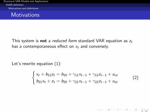
This system is not a reduced form standard VAR equation as zt

has a contemporaneous effect on xt and conversely.

Let’s rewrite equation (1):xt + b12zt = b10 + γ11xt−1 + γ12zt−1 + uxt

b21xt + zt = b20 + γ21xt−1 + γ22zt−1 + uzt(2)

6 / 38


SVAR definition


Motivations

Then in a matricial form:

B−1yt = Γ0 + Γ1yt−1 + ut , (3)

with : y ′t = (xt , zt), Γ′0 = (b10, b20) and u′t = (uxt , uzt)and :

B−1 =

(1 b12

b21 1

)

Γ1 =

(γ11 γ12

γ21 γ22

)

7 / 38


SVAR definition


Recall

If we assume M is a 2× 2 matrix such as :

M =

(a bc d

)

If ad − bc 6= 0 then M can be inverted and

M−1 =1

ad − bc

(d −b−c a

)

8 / 38


SVAR definition


Motivations

Assuming B−1 is inversible, by multiplying by B the primitive formcan be rewritten in its reduced form:

yt = A0 + A1yt−1 + εt (4)

withA0 = BΓ0,

A1 = BΓ1,

εt = But

9 / 38


SVAR definition


Motivations

Thus the reduced form can be rewritten as :xt = a10 + a11xt−1 + a12zt−1 + εxt

zt = a20 + a21xt−1 + a22zt−1 + εzt(5)

where residuals εt are linear combinations of the 2 structuralshocks such as:

εxt =1

1− b21b12(uxt − b12uzt)

εzt =1

1− b21b12(uzt − b12uxt)

(6)

10 / 38


SVAR definition


Properties of εt

We can show that

1

E (εxt) = E (εzt) = 0

2

E (ε2xt) =

1

(1− b12b21)2(σ2

x + b212σ

2z )

E (ε2zt) =

1

(1− b12b21)2(σ2

z + b221σ

2x )

3 For all j 6= 0 :E (εxtεx ,t−j ) = 0

E (εztεz,t−j ) = 0

11 / 38


SVAR definition


Properties of εt

What about covariance? We can show that:

E (εxtεzt) = − 1

(1− b12b21)2(b21σ

2x + b12σ

2z )

In general, non-null covariance except if b12 = b21 = 0, that is nocontemporaneous effect.

Covariance matrix Ω such that:

Ω =

(E (ε2

xt) E (εxtεzt)E (εxtεzt) E (ε2

zt)

)

12 / 38


SVAR definition


Identification issue

The residuals εt have good properties, meaning that the reducedform can be efficiently estimated.

Question: Is it possible to recover all the information present inthe primitive form from the estimation of the reduced form ?

Answer: NO ! 9 parameters in the reduced form but 10parameters in the primitive form : The system is not fully identified

13 / 38


SVAR definition


Identification issue

Solution (Sims, 1980): recursive identification scheme, ie :recursive system with restrictions on the primitive form.Ex. Assume zt does not have any contemporanesous effect on xt ,ie : b21 = 0Thus B−1 is a lower diagonal matrix:

B−1 =

(1 0b21 1

)Alternative: b12 = 0, ie: xt has no effect on zt

Main issue in SVAR modelling: how to define B−1 ?

14 / 38


SVAR definition

Causal mechanisms

Causal mechanisms in a stylized economy

IRFs from SVAR with Inflation, Unemployment and FFR

15 / 38


SVAR definition

Causal mechanisms


Assume that the GDP growth gt is affected by some realshocks ur ,t following:

gt = −0.3(it−1 − πt) + ur ,t

where it is the nominal interest rate, πt is the inflation rate.

Besides, assume that we have a simple Taylor rule governingshort-term interest rates :

it = 0.9it−1 + 1.5πt + ump,t

where ump,t is a monetary-policy shock.

The inflation rate is supposed to follow a backward-lookingPhillips curve:

πt = 0.9πt−1 + 0.2gt−1 + un,t

where un,t is a cost-push shock.16 / 38


SVAR definition

Causal mechanisms


The structural shocks ut = (ur ,t , ump,t , un,t) are uncorrelated(i.e., the covariance matrix of ut , denoted with Ωu is diagonal)

The structural shocks ut are serially uncorrelated (i.e.Cov(ut−k , ut) = 0 for any t and k > 0).

17 / 38


SVAR definition

Causal mechanisms


The “structural” model readsgt = −0.3(it−1 − πt) + ur ,t

it = 0.9it−1 + 1.5πt + ump,t

πt = 0.9πt−1 + 0.2gt−1 + un,t .

To get it in a “reduced-form”, let us substitute πt in theright-hand sides of the first two equations:

gt = 0.06gt−1 − 0.3it−1 + 0.27πt−1 + 0.3un,t + ur ,t

it = 0.9it−1 + 1.35πt−1 + 0.3gt−1 + ump,t + 1.5un,t

πt = 0.9πt−1 + 0.2gt−1 + un,t .

18 / 38


SVAR definition

Causal mechanisms


In matrix form gt

itπt

=

0.06 −0.3 0.270.3 0.9 1.350.2 0 0.9

gt−1

it−1

πt−1

+

εg ,t

εi ,t

επ,t

with

εg ,t

εi ,t

επ,t

=

1 0 0.30 1 1.50 0 1

ur ,t

ump,t

un,t

= B

ur ,t

ump,t

un,t

.

With the procedure described above, one only gets anestimate of Ωε where

Ωε = Var

εg ,t

εi ,t

επ,t

.

19 / 38


Identification issues

Identification in SVAR

We saw that a structural model can be thought in its general form :

εt = yt − E(yt |It−1), (7)

withεt = But (8)

In our case of SVAR(p), equation (7) is:

yt = A0 +

p∑i=1

Aiyt−i + εt , (9)

orA(L)yt = εt , (10)

20 / 38



SVAR: Orthogonalization

Estimation of AR parameters via MLE then estimation ofstructural parameters in B

Note that we must have

Ωε = BΩuB′

where Ωu is diagonal positive such as: Ωu = I.

In addition, given the “structural” framework, one knows thatB is a triangular matrix (lower or upper according to thespecification).

21 / 38



SVAR: Orthogonalization

It has been shown previously that a SVAR is a structuralmodel that draws from a theoretical framework.

As a starting point, we always have Ωε = BΩuB′ that provides

us with n(n + 1)/2 restrictions to recover the B matrix.

Consequently, to get the B matrix, one have to imposen(n − 1)/2 additional restrictions.

22 / 38



SVAR: Restrictions

There exist several restrictions that can be implemented in aSVAR:

a short-run restriction prevents a structural shock fromaffecting an endogenous variable contemporaneously bysetting to zero some entries of B.

a long-run restriction prevents a structural shock fromaffecting an endogenous variable in a cumulative way.

a sign restriction imposes negative or positive parameters inmatrix B.

23 / 38



SVAR: Short-Run restrictions

Short-run restrictions are simpler to implement than the otherones.

There are particular cases in which some well-known matrixdecompostion can be used to easily estimate some specificSVAR.

Imagine a context in which you can argue that there exists an“ordering” of the shocks:

A first shock structural u1,t can affect instantaneously (i.e., int) only one of the endogenous variable (say, y1,t) through ε1,t ;A second shock, u2,t can affect instantaneously the first twoendogenous variables (say, y1,t and y2,t) through ε1,t and ε2,t ;...

24 / 38




Within this framework, the structural recursive mechanism ofvariable ordering allows the creation of the lower-triangular Bmatrix:

ε1,t = u1,t

ε2,t = β21u1,t + u2,t

ε3,t = β31u1,t + β32u2,t + u3,t

. . . = . . .

εn,t = βn1u1,t + . . .+ βn,n−1un−1,t + un,t

where the ut are the structural shocks and are notcross-correlated at all leads and lags.

25 / 38




The triangular structural model imposes the recursive causalordering:

y1 → y2 → . . .→ yn

y1 causes y2, y3, . . . , yn

but y2, y3, . . . , yn do not cause y1

y2 causes y3, . . . , yn

but y3, . . . , yn do not cause y2

...

Obviously, a different ordering of variables leads to a different result

26 / 38



Cholesky decomposition/factorization

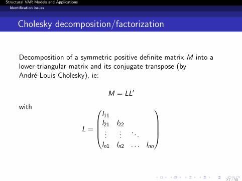
Decomposition of a symmetric positive definite matrix M into alower-triangular matrix and its conjugate transpose (byAndre-Louis Cholesky), ie:

M = LL′

with

L =

l11

l21 l22...

.... . .

ln1 ln2 . . . lnn

27 / 38



Cholesky decomposition/factorization

Property:The ML estimate of B is the Cholesky decomposition of Ωε thesample covariance matrix of VAR residuals.

If the model is just-identified, Ωε(BB′)−1 = In and the

log-likelihood simplifies to:

L = Const − 0.5 log |Ωε| − 0.5n

28 / 38



IRF for SVAR

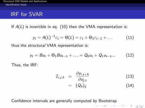
If A(L) is invertible in eq. (10) then the VMA representation is:

yt = A(L)−1εt = Θ(L) = εt + Θ1εt−1 + . . . (11)

thus the structural VMA representation is:

yt = But + Θ1But−1 + . . . = Q0ut + Q1ut−1... (12)

Thus, the IRF:

Ii ,j ,h =∂yi ,t+h

∂uj ,t(13)

= (Qh)ij (14)

Confidence intervals are generally computed by Bootstrap

29 / 38



Forecast Error Variance Decomposition

FEV after h steps:

Ωh =h∑

k=0

QkQ′k (15)

Hence the variance vi for yi is :

vi = (Ωh)ii =h∑

k=0

e ′iQkQ′kei =

h∑k=0

n∑l=1

(qki ,l )

2

where ei is a zero-vector with 1 at the i th element and (qki ,l )

2 is the(i , l) element of Qk .Thus the share of variance on yi attributed to the j th shock after hperiods is:

VDi ,j ,h =

∑hk=0(qk

i ,l )2∑h

k=0

∑nl=1(qk

i ,l )2

30 / 38


Applications

Cholesky decomposition: Illustration

Dedola and Lippi (“The Monetary Transmission Mechanism:Evidence from the Industries of Five OECD Countries”, 2005)estimate 5 SVAR for the US, the UK, Germany, France andItaly to analyse the monetary-policy transmission mechanisms

SVAR(p = 5) estimation over the period 1975-1997

Identification scheme is based on Cholesky decompositions,the ordering of the endogenous variables being: the industrialproduction, the consumer price index, a commodity priceindex, the short-term rate and a monetary aggregate (exceptfor the US).

This ordering implies that monetary policy reacts to theshocks affecting the first three variables but that the latterreact to monetary policy with a one-period lag.

31 / 38


Applications

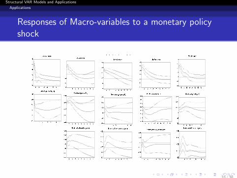
Responses of Macro-variables to a monetary policyshock

Figure 1

Responses of the main macro variables to a monetary policy shock!±"#$%&'(&)(#*))+)#,&'($-

Note: The boxes in each column show the response of the VAR variables to a shock to the short term interest rate (equal toone standard deviation) yielded by the SVAR estimates of Table 1. The error bands were computed with Monte Carlosimulations. The horizontal axis reports the months elapsed since the interest rate shock.

32 / 38


Applications

Responses of Macro-variables to a monetary policyshock

Figure 1

Responses of the main macro variables to a monetary policy shock!±"#$%&'(&)(#*))+)#,&'($-

Note: The boxes in each column show the response of the VAR variables to a shock to the short term interest rate (equal toone standard deviation) yielded by the SVAR estimates of Table 1. The error bands were computed with Monte Carlosimulations. The horizontal axis reports the months elapsed since the interest rate shock. 33 / 38


Applications

Kilian (2009)

“Not all shocks are alike: Disentangling demand from supplyshocks in the crude oil market” AER.

Objective: Distinct effects of supply and demand shocks on oilprices

Methodology: A structural monthly VAR is used to identifyaggregate supply of oil, aggregate demand of oil andprecautionary shocks

Findings: Precautionary shocks have adverse effects on oilprices .

34 / 38


Applications

Kilian (2009)

Data

Global oil production

Global demand estimated by monthly industrial commoditites

Real price of oil

Model:

A0yt = α +24∑

i=1

Aiyt−1 + εt

whereyt = (∆Prodt , reat , rpot)

′

35 / 38


Applications

Kilian (2009)

uProd ,t

uRea,t

uRpo,t

=

a11 0 0a21 a22 0a31 a32 a33

εOilsupply ,t

εAggregatedemand ,t

εOilspecific,t

36 / 38


Applications

37 / 38


Applications

References

Blanchard, O. and Quah, D. (1989). The Dynamic Effects of AggregateDemand and Supply Disturbances. American Economic Review , vol. 79.

Dedola, L. and Lippi, F. (2005). The monetary transmission mechanism:Evidence from the industries of five OECD countries. European EconomicReview , vol. 49 (6).

Gerlach, S. and F. Smets (1995). The monetary transmission mechanism:evidence from the G7 countries. CEPR Discussion Paper, no. 1219.

Hamilton, J. (1994). Time Series Analysis. Princeton University Press.

Kilian, L. (2009. Not all shocks are alike: Diesntangling supply fromdemand shocks on the crude oil marketAmerican Economic Review , vol.

Sims, C. (1980). Macroeconomics and Reality. Econometrica, vol. 48.

Smets, F. and Tsatsaronis, K. (1997). Why does the yield curve predicteconomic activity? BIS Working Paper No. 49.

38 / 38

Structural VAR Models and Applications - … · 2016-10-23 · the primitive form from the...

Documents

Transcript of Structural VAR Models and Applications - … · 2016-10-23 · the primitive form from the...