STRUCTURAL HEALTH MONITORING USING...

STRUCTURAL HEALTH MONITORING USING ADAPTIVE

WAVELET FUNCTIONS

SEYED HOSSEIN MAHDAVI

THESIS SUBMITTED IN FULFILLMENT

OF THE REQUIREMENTS

FOR THE DEGREE OF DOCTOR OF PHILOSOPHY

FACULTY OF ENGINEERING

UNIVERSITY OF MALAYA

KUALA LUMPUR

2016

ii

UNIVERSITY OF MALAYA

ORIGINAL LITERARY WORK DECLARATION

Name of Candidate: Seyed Hossein Mahdavi (I.C/Passport No: I 95756720 )

Registration/Matric No: KHA120002

Name of Degree: PHD

Title of Project Paper/Research Report/Dissertation/Thesis (“this Work”):

STRUCTURAL HEALTH MONITORING USING ADAPTIVE WAVELET

FUNCTIONS

Field of Study:

I do solemnly and sincerely declare that:

(1) I am the sole author/writer of this Work;

(2) This Work is original;

(3) Any use of any work in which copyright exists was done by way of fair dealing

and for permitted purposes and any excerpt or extract from, or reference to or

reproduction of any copyright work has been disclosed expressly and sufficiently

and the title of the Work and its authorship have been acknowledged in this Work;

(4) I do not have any actual knowledge nor do I ought reasonably to know that the

making of this work constitutes an infringement of any copyright work;

(5) I hereby assign all and every rights in the copyright to this Work to the University

of Malaya (“UM”), who henceforth shall be owner of the copyright in this Work

and that any reproduction or use in any form or by any means whatsoever is

prohibited without the written consent of UM having been first had and obtained;

(6) I am fully aware that if in the course of making this Work I have infringed any

copyright whether intentionally or otherwise, I may be subject to legal action or

any other action as may be determined by UM.

Candidate’s Signature Date:

Subscribed and solemnly declared before,

Witness’s Signature Date:

Name:

Designation:

iii

ABSTRACT

In this study, two aspects of structural dynamic problems have been considered, involving

direct structural dynamics as well as inverse problems. The first part of this research is

directed towards improving an explicit and indirect time integration method for structural

dynamic problems capable of using adaptive wavelets. The developed scheme is

comprehensive enough for use with any wavelet basis function. To investigate the

applicability of different wavelet functions for different problems, in particular, the simple

family of Haar wavelets, the complex and free-scaled Chebyshev wavelets of the first (FCW)

and second kind (SCW) and Legendre wavelets (LW) have been evaluated. A detailed

assessment is carried out on the stability, accuracy and computational efficiency of responses

calculated by Haar wavelet, FCW, SCW and LW. The proposed method lies on an

unconditionally stable scheme, hence, there is no requirement on the selection of the time

interval. This allowed the numerical procedure to be performed on long time increments.

Practically, an efficient structural health monitoring strategy is the resultant of the

implementation of an enhanced structural simulation through inverse problem approach. As

a consequence, the computational performance of structural health monitoring strategies will

be directly influenced by the higher computational competency and convergence rate of the

proposed wavelet-based method for structural simulation.

Accordingly, in the second part of this research, the procedure of structural identification

and damage detection has been developed by employing the wavelet-based method through

the modified genetic algorithms (GAs) to optimally solve inverse problems. For this purpose,

a wavelet-based GAs strategy is improved by using free-scaled adaptive wavelets to

optimally identify unknown structural parameters. The appropriateness and effectiveness of

the proposed strategy have been evaluated both numerically and experimentally. The

iv

numerical assessment demonstrated the robustness of the proposed technique for

identification and damage detection of large-scaled structures with the best performance. For

the experimental validation, three test setups were conducted for identification and damage

detection, including two different MDOF systems and a 2-dimentional truss structure.

Consequently, it was shown that the computational efficiency of structural identification and

relatively, damage detection strategies were significantly enhanced. This led the optimum

results with the highest accuracies and provided the sufficiently reliable strategy in assessing

the structural integrity, safety and reliability.

v

ABSTRAK

Melalui kajian ini, pihak pengkaji telah menitikberatkan dua aspek masalah dinamik

struktur, yakni yang melibatkan dinamik struktur secara terus dan masalah songsangan.

Bahagian pertama kajian ini adalah menjurus ke arah meningkatkan kaedah integrasi masa

yang nyata dan secara tidak langsung untuk masalah struktur dinamik yang mampu

menggunakan penyesuaian gelombang kecil (wavelet). Skim yang disediakan cukup

komprehensif untuk digunakan dengan sebarangan fungsi asas wavelet. Bagi Menyiasat

penggunaan / keterterapan fungsi gelombang kecil (wavelet) yang berbeza untuk masalah

yang berbeza, terutamanya, keluarga mudah (riak) wavelet Haar, wavelet Chebyshev pertama

(FCW) yang kompleks dan berskala bebas dan jenis kedua (SCW) serta wavelet Legendre

(LW) telah dinilai. Satu penilaian terperinci telah dijalankan terhadap kestabilan, ketepatan

dan kecekapan dalam pengiraan tindak balas yang telah dikira dengan menggunakan wavelet

Haar, FCW, SCW dan LW. Kaedah yang dicadangkan bergantung kepada skim yang stabil

tanpa syarat, walhal, tidak ada keperluan terhadap pemilihan selang masa. Ini telah

membolehkan prosedur berangka yang dilakukan ke atas pertambahan masa yang panjang.

Secara praktikalnya, struktur strategi pemantauan kesihatan yang cekap adalah paduan

pelaksanaan simulasi struktur yang telah dipertingkatkan melalui pendekatan masalah

songsang. Akibatnya, prestasi pengkomputeran strategi pemantauan kesihatan struktur akan

terus dipengaruhi oleh kecekapan pengiraan dan penumpuan pada kadar yang lebih tinggi

daripada kaedah berasaskan gelombang kecil (wavelet) yang dicadangkan untuk simulasi

struktur.

Oleh itu, dalam bahagian kedua kajian ini, prosedur mengenalpasti struktur dan

pengesanan kerosakan telah dibentuk dengan menggunakan kaedah berasaskan wavelet-

melalui algoritma genetik yang telah diubahsuai (GA) bagi menyelesaikan masalah songsang

vi

secara optimum. Bagi tujuan ini, strategi GA berasaskan wavelet telah dipertingkatkan

dengan menggunakan riak (wavelet) penyesuaian bebas untuk meningkatkan keupayaannya

dalam mengenalpasti secara optimum parameter struktur yang tidak diketahui. Kesesuaian

dan keberkesanan strategi yang dicadangkan telah dinilai secara berangka dan uji kaji.

Penilaian berangka menunjukkan keteguhan teknik yang dicadangkan untuk pengenalan dan

pengesanan kerosakan struktur berskala besar yang mempunyai prestasi terbaik. Untuk

pengesahan eksperimen, persediaan tiga ujian telah dijalankan untuk mengenalpasti dan

mengesan kerosakan, termasuklah dua sistem MDOF yang berbeza dan struktur kekuda 2-

dimensi. Oleh yang demikian, ia menunjukkan bahawa kecekapan pengiraan dalam

pengenalan struktur dan secara relatifnya, strategi pengesanan kerosakan telah

dipertingkatkan dengan ketara. Ini telah menghasilkan keputusan yang optimum dengan

ketepatan tertinggi dan menjamin strategi yang cukup dipercayai dalam menilai keutuhan,

keselamatan dan kebolehpercayaan struktur tersebut.

vii

ACKNOWLEDGMENTS

Praise and thank Almighty God for giving me the wisdom, health and strength to complete

this research.

I would like to express my deepest gratitude and appreciation to my supervisor, Prof. Dr.

Hashim Abdul Razak for his kind supervision, valuable guidance, encouragement, and

immense assistance throughout the preparation of this work.

I also would like to acknowledge the financial supports provided by the University of

Malaya through the Bright Spark scholarship scheme (Scholarship no.: BSP/APP/1818/2013)

and PPP research grant PG078-2013B.

Also, I express my deepest appreciation to the staff of Department of Civil Engineering,

and the Faculty of Engineering, University of Malaya, for their kind help during my work,

which has resulted in reaching my research objectives on schedule.

Finally, I wish to give my heartfelt and special thanks to my family; my parents, wife and

son for their patience, encouragement and unwavering supports throughout the duration of

my studies.

Seyed Hossein

February 2016

viii

TABLE OF CONTENTS

Original literary work declaration .......................................................................................... ii

Abstract ................................................................................................................................. iii

Abstrak ................................................................................................................................... v

Acknowledgments ................................................................................................................ vii

Table of contents ................................................................................................................. viii

List of figures ....................................................................................................................... xii

List of tables ........................................................................................................................ xxi

List of symbols and abbreviations ..................................................................................... xxiv

CHAPTER 1: INTRODUCTION ....................................................................................... 1

1.1 General ............................................................................................................................. 1

1.2 Objectives and problem statement ................................................................................... 3

1.3 Scope of study .................................................................................................................. 6

1.4 Organization of thesis..................................................................................................... 11

CHAPTER 2: LITERATURE REVIEW ......................................................................... 13

2.1 Introduction .................................................................................................................... 13

2.2 Background of wavelet analysis ..................................................................................... 13

2.2.1 Mathematical transforms ......................................................................................... 14

2.2.2 Family of Fourier transforms ................................................................................... 15

2.2.3 Wavelet transforms .................................................................................................. 19

2.3 Structural dynamics simulation (direct or forward analysis) ......................................... 21

2.4 Structural identification (inverse analysis) ..................................................................... 24

2.4.1 Frequency domain methods ..................................................................................... 25

2.4.1.1 Frequency based methods ................................................................................. 25

2.4.1.2 Mode shape based methods .............................................................................. 28

2.4.2 Time domain methods ............................................................................................. 29

2.4.2.1 Classical methods.............................................................................................. 29

ix

2.4.2.2 Non-classical methods ...................................................................................... 31

2.5 Applications of wavelet functions .................................................................................. 35

2.5.1 Structural simulation (direct or forward analysis) ................................................... 35

2.5.2 Structural identification and damage detection ....................................................... 39

2.6 Discussion ...................................................................................................................... 42

2.7 Chapter summary ........................................................................................................... 44

CHAPTER 3: STRUCTURAL DYNAMICS .................................................................. 47

3.1 Introduction .................................................................................................................... 47

3.2 Solution of direct problems (forward analysis) .............................................................. 48

3.2.1 Fundamentals of wavelet analysis ........................................................................... 48

3.2.1.1 2D Haar wavelet functions................................................................................ 49

3.2.1.2 First kind of 3D Chebyshev wavelets ............................................................... 51

3.2.1.3 Second kind of 3D Chebyshev wavelets ........................................................... 52

3.2.1.4 3D Legendre wavelets ....................................................................................... 53

3.2.1.5 Functional decomposition and operational matrix of integration ..................... 54

3.2.1.6 Comparison of 2D and 3D wavelet functions ................................................... 60

3.2.2 The proposed method for dynamic analysis of SDOF structures ............................ 65

3.2.3 The proposed method for dynamic analysis of MDOF structures........................... 68

3.3 Stability analysis of the wavelet-based method ............................................................. 72

3.4 Accuracy analysis of the wavelet-based scheme............................................................ 76

3.4.1 First ordered operation of integration ...................................................................... 76

3.4.2 Second ordered operation of integration ................................................................. 78

3.4.3 Functional approximation ........................................................................................ 80

3.5 The proposed method for operation of derivative .......................................................... 82

3.6 Numerical verifications .................................................................................................. 87

3.6.1 A set of mass-spring system .................................................................................... 87

3.6.2 MDOF shear building .............................................................................................. 91

3.6.3 A double layer Barrel truss structure ....................................................................... 94

3.6.4 Large scaled 3D spherical truss structure subjected to impact ................................ 98

3.7 Chapter Summary ......................................................................................................... 101

CHAPTER 4: INVERSE PROBLEMS .......................................................................... 104

x

4.1 Introduction ............................................................................................................. 104

4.2 Stiffness identification of SDOF systems ............................................................... 105

4.2.1 Optimum measurement of displacement and velocity from acceleration ........... 105

4.2.2 Optimum measurement of acceleration derivatives ............................................ 107

4.2.3 Stiffness identification ......................................................................................... 109

4.3 Structural identification of MDOF systems using genetic algorithms .................... 111

4.3.1 Simple GAs ......................................................................................................... 113

4.3.1.1 Fitness evaluation and selection...................................................................... 115

4.3.2 Modified multi-species GAs ................................................................................ 118

4.3.3 Wavelet-based MGAs.......................................................................................... 118

4.3.3.1 Modification of multi-species populations ..................................................... 119

4.3.3.2 Modified search space reduction technique .................................................... 124

4.3.3.3 Fitness evaluation and artificial selection ....................................................... 126

4.3.3.4 Practical algorithm of WMGA strategy .......................................................... 127

4.4 Modification of WMGA strategy for output-only identification ............................ 130

4.5 WMGA strategy for structural damage detection ................................................... 132

4.6 Numerical verification study ................................................................................... 134

4.6.1 A MDOF shear building ...................................................................................... 136

4.6.2 A 2D truss structure ............................................................................................. 148

4.6.3 A large-scaled 3D truss structure......................................................................... 156

4.7 Chapter summary .................................................................................................... 163

CHAPTER 5: EXPERIMENTAL VERIFICATION ................................................... 167

5.1 Introduction ............................................................................................................. 167

5.2 Experiment 1 - A MDOF shear structure subjected to the base acceleration ......... 168

5.2.1 Preliminary measurements and calculations ....................................................... 170

5.2.2 Main identification test ........................................................................................ 173

5.2.3 Results and discussion ......................................................................................... 174

5.3 Experiment 2 - A MDOF shear structure under nodal excitation ........................... 178


5.3.2 Main identification and damage detection test .................................................... 185


5.4 Experiment 3 - A 2D truss structure under nodal excitation ................................... 194

xi


5.4.2 Main identification and damage detection test .................................................... 201


5.5 Chapter summary .................................................................................................... 210

CHAPTER 6: CONCLUSIONS AND RECOMMENDATIONS ................................ 212

6.1 Introduction ............................................................................................................. 212

6.2 Structural simulation (forward analysis) ................................................................. 212

6.3 Structural health monitoring (inverse analysis) ...................................................... 215

6.4 Recommendations ................................................................................................... 218

6.4.1 Future work direction .......................................................................................... 219

APPENDICES .................................................................................................................. 220

Appendix A: Static and dynamic condensation procedures ............................................... 220

A.1 Guyan static condensation method (GSC)........................................................... 220

A.2 Guyan dynamic condensation method (GDC) .................................................... 221

Appendix B: Optimum sensor placement .......................................................................... 223

Appendix C: Optimum node numbering of large-scaled structures ................................... 224

Appendix D: Structural simulation results ......................................................................... 226

D.1 A four nodes quadrilateral element ..................................................................... 226

D.2 A plane stress system discretized into CST elements ......................................... 229

Appendix E: Structural identification and damage detection results ................................. 232

E.1 A simulated SDOF system .................................................................................. 232

E.2 Optimum measurement of structural responses of a SDOF model ..................... 239

E.3 A 2D truss constructed with bar elements coupled with damage ........................ 244

E.4 Stiffness identification results for Case (c), Ex. 4.6.1, Chapter 4 ………...……250

E.5 Truss structure considered in Chapter 5 .............................................................. 250

REFERENCES ................................................................................................................. 253

LIST OF PUBLICATIONS AND PAPERS PRESENTED ......................................... 266

xii

LIST OF FIGURES

Figure 1.1: (a) Structural simulation (direct); (b) structural identification (inverse). ........... 1

Figure 1.2: The proposed iterative algorithm for solving structural dynamics problems using

adaptive wavelet functions. ................................................................................... 9

Figure 1.3: Overall schematic view of methodology utilized in this study for solving inverse

problems. ............................................................................................................. 10

Figure 1.4: The scope of numerical and experimental work for inverse analysis. .............. 11

Figure 2.1: The schematic view of operation of transforms ............................................... 15

Figure 3.1: Different scales of Haar wavelets as scaled and transitioned pulse functions.. 50

Figure 3.2: (a) Weight functions, (b) shape functions for the 8th and 12th order, (c) shape

functions for the 8th and 12th order corresponding to the first (𝑻𝒏(𝒙)) and second

((𝑼𝒏(𝒙)) kind of Chebyshev polynomials. ......................................................... 52

Figure 3.3: The mth degree of Chebyshev polynomials of the first (Tm(t)) and second kind

(Um(t)) and Legendre polynomials (Lm(t)). (a) m=8, (b) m=2. ........................... 54

Figure 3.4: Comparison of the first 8th scales of wavelet functions, (a) 2D Haar family, (b)

3D Chebyshev polynomial. ................................................................................. 62

Figure 3.5: Approximation of F(t) and wavelet coefficients for the first 8th scale of (a) FCW,

(b) Haar wavelet, at the first second of F(t) and 𝝎=8 rad/sec (CH_CW=

coefficients of FCW, HA_CW= coefficients of Haar wavelet, App. of

F(t)_CH/HA= approximation of F(t) using Chebyshev/Haar wavelet). .............. 63


(b) Haar wavelet, for the first second of F(t) and 𝝎=15 rad/sec (CH_CW=

coefficients of FCW, HA_CW= coefficients of Haar wavelet, App. of

F(t)_CH/HA= approximation of F(t) using Chebyshev/Haar wavelet). .............. 63

xiii


(b) Haar wavelet, for the first second of F(t) and 𝝎=500 rad/sec (CH_CW=

coefficients of FCW, HA_CW= coefficients of Haar wavelet, App. of F(t)_CH=

approximation of F(t) using FCW, App. of F(t)_HA(2M8/128)= approximation of

F(t) using the first 8/128th scale of Haar wavelet). .............................................. 65

Figure 3.8: Comparison of spectral radius for the proposed method and another four

integration schemes. ............................................................................................ 75

Figure 3.9: Comparison of spectral radius calculated for the second scale of FCW, SCW and

LW. ...................................................................................................................... 76

Figure 3.10: PTARE corresponding to the considered first-ordered differential equation and

relative computational time of FCW, SCW and LW using the first 4th, 6th and 64th

SM collocation points related to the scales of wavelets (M=SM points/2). ........ 77

Figure 3.11: Error measurment. (a) Period elongation (PE=(T-T0)/T0). (b) Amplitude decay

(AA= average acceleration, LA= linear acceleration of Newmark-β family). .... 79

Figure 3.12: Comparison of the approximation of F(t)=100sin(𝝎t) for 𝝎=5 and 30rad/sec

(App-F(t)), the original F(t) and the scaled wavelet coefficients corresponding to

the first 8th and 32nd scales of FCW, SCW and LW. ........................................... 81

Figure 3.13: The approximated results using the proposed operation of derivative of FCW

on 𝟐𝑴=8 collocation points for calculation of (a) the first, (b) the second

derivative. ............................................................................................................ 84

Figure 3.14: The approximated results using the proposed operation of derivative of SCW

on 𝟐𝑴=8 collocation points for computation of (a) the first, (b) the second

derivative. ............................................................................................................ 85

Figure 3.15: PTARE measurement corresponding to different scales (𝟐𝑴 collocations) of

FCW. ................................................................................................................... 86

Figure 3.16: PTARE measurement corresponding to various scales (𝟐𝑴 collocations) of

SCW. ................................................................................................................... 86

Figure 3.17: 21 DOF mass spring system vibrated by sinusoidal load (load frequency=8𝝅

Hz), ∆𝐭=0.05 sec. ................................................................................................. 88

xiv

Figure 3.18: The first 10 sec horizontal displacement time-history of 7th mass, shown in

Figure 3.17. .......................................................................................................... 89

Figure 3.19: Total average errors in displacement of 7th mass, shown in Figure 3.17 and

relative computation time involved (CH= First kind of Chebyshev wavelet, CD=

central difference, LA=linear acceleration). ........................................................ 90

Figure 3.20: A thirty story shear building under El-Centro acceleration. ........................... 91

Figure 3.21: Displacement time-history of story 5, shown in Figure 3.20. ........................ 92

Figure 3.22: PTARE in time-history displacement of story 5, shown in Figure 3.20 and

corresponding computational time (CD=central difference, LA=linear

acceleration). ....................................................................................................... 93

Figure 3.23: Double layer and pin-jointed Barrel space structure under two concentrated

impacts. ................................................................................................................ 95

Figure 3.24: Vertical time-history of displacements of the node under impact 1, at the bottom

layer shown in Figure 3.23. ................................................................................. 97

Figure 3.25: A double layer and spherical space structure (bar elements) subjected to two

shock loadings. .................................................................................................... 99

Figure 3.26: Vertical time-history displacement of node 1 shown in Figure 3.25, (a) the first

2 seconds after impact, (b) 0.5-1sec after impact (LA=linear acceleration, HHT-

α=Hilber-Hughes-Taylor). ................................................................................. 100

Figure 3.27: Percentile total average errors in vertical displacement of node 1, shown in

Figure 3.25 and relative computation time involved. (CH(2Mµ)= µ scale of SCW,

LA=linear acceleration, HHT-α=Hilber-Hughes-Taylor). ................................ 101

Figure. 4.1: The magnificent sensitivity of jerk using the wavelet operators on optimum

collocations compared with the normal incremental procedure. ....................... 110

Figure 4.2: The proposed approaches capable of using adaptive wavelets through GAs, (a)

for initial and rough identification, (b) for accurate and reliable identification. 112

xv

Figure 4.3: Overall layout of a simple GA. ....................................................................... 114

Figure 4.4: Representation and storage of a simple GAs for the identification problems

comprised of n structural elements. ................................................................... 114

Figure 4.5: The construction of the proposed multi-species population capable of using

WMGA. ............................................................................................................. 119

Figure 4.6: The proposed SSRM strategy capable of using adaptive wavelets for optimum

identification through WMGA. ......................................................................... 125

Figure 4.7: The proposed WMGA strategy by using adaptive wavelet functions. ........... 128

Figure 4.8: The practical flowchart to optimally simulate dynamic response using wavelet

functions prior to fitness evaluation (FE) of genetic individuals (Ind). ............ 129

Figure 4.9: The proposed algorithm for damage detection strategy using WMGA. ......... 133

Figure 4.10: MDOF shear building, (a) the entire three connected structures, (b) structural

identification of the central structure under two known forces, (c) structure

extracted for force identification. ...................................................................... 139

Figure 4.11: Total average error (%) in stiffness values and computation time involved for

different sensor placements (known and unknown mass identification). ......... 142

Figure 4.12: Simulated time-history of acceleration (Acc) and displacement (Disp)

corresponding to the 9th, 6th and 4th levels; the full measurement of Case (c). . 146

Figure 4.13: Force identification of Case (c) shown in Figure 4.10 (O-only and full

measurement). ................................................................................................... 147

Figure 4.14: A 2D camel back pin-jointed truss structure considered for Example 4.6.2. 150

Figure 4.15: The convergence history of percentile maximum error in identification of

stiffness for WMGA and MGA. ........................................................................ 151

xvi

Figure 4.16: The percentile total average of maximum errors and computation time involved

for SGA, WMGA and MGA. ............................................................................ 153

Figure 4.17: The large-scaled hexagonal space structure under concentrated loadings

considered for Example 4.6.3. ........................................................................... 158

Figure 4.18: The percentile maximum errors and computation time involved recorded for

RMGA and WMGA corresponding to different sensor placement (SP) and loading

(Lo) scenarios. ................................................................................................... 160

Figure 4.19: Damage detection success % (location and magnitude) using WMGA for

different sensor placements (SP), loadings (Lo) and damage scenarios (DS); (a)

DS1, (b) DS2, (c) DS2 (presented in Tables 4.13 and 4.14). ............................ 164

Figure 5.1: The schematic view of test setup in lab for output-only identification of the

flexible MDOF shear system, (a) large shaking MDOF shear system at the base

(S(t): base acceleration), (b) fixed support at the base for impact test, (c)

dimensions (cm). ............................................................................................... 169

Figure 5.2: The schematic view of static test performed in lab for the first MDOF system

(O-only identification). ...................................................................................... 171

Figure 5.3: Time-history of acceleration (the first 4000 points) corresponding to, (a) story 4,

(b) story 3, (c) story 2, (d) story 1, (e) S(t): the base acceleration (g = 9.81 m/sec2).

........................................................................................................................... 175

Figure 5.4: Time-history of identified force (500 to 750 acquired points) corresponding to,

(a) story 2, (b) story 3. ....................................................................................... 176

Figure 5.5: The percentile total average error of identified force and the mean error (%) in

identified stiffness of each story for output-only measurement. ....................... 177

Figure 5.6: The schematic view of the test setup: (a) the laboratory aluminum MDOF shear

building, (b) dimensions of the frame (m), (c) dimensions of the columns (m), (d)

dimensions of the rigid beam (m). ..................................................................... 179

Figure 5.7: The schematic view of static test conducted in lab. ....................................... 181

xvii

Figure 5.8: Power spectrum of response at fourth story due to impact at that story. ........ 182

Figure 5.9: Damage scenarios and relative finite element models to estimate damage index

(%), (a) undamaged column, (b) small damage, (c) large damage (dimensions are

given in cm). ...................................................................................................... 184

Figure 5.10: Test setup and instruments used in lab, (a) main test setup, (b) shaker

installation, top view, (c) accelerometer installation, side view. ...................... 186

Figure 5.11: The schematic diagram of data acquisition and test setup............................ 186

Figure 5.12: Total average error and computation time involved for stiffness identification

of undamaged MDOF system shown in Figure 5.6 (known/unknown mass

problems and full measurement). ...................................................................... 189

Figure 5.13: Success in identified damage index for different damage scenarios,

known/unknown mass problems and incomplete measurement (DOFs represents

measured DOFs). ............................................................................................... 191

Figure 5.14: The schematic view of the test setup for Experiment 3: (a) the laboratory 2D

truss, (b) sensor placement, (c) dimensions of the truss (cm), node and element

numbering, (d) new nodes and elements for the progressive damage detection

strategy, (e) section details (cm). ....................................................................... 196

Figure 5.15: The first six mode shapes and natural frequencies obtained from FE model of

2D truss structure. .............................................................................................. 197

Figure 5.16: Power spectrum of response at DOF 4-y due to impact at 4-y (shown in Figure

5.14). .................................................................................................................. 198

Figure 5.17: Damage scenarios imposed to the 2D truss, (a) large damage on element 4

shown in Figure 5.14, (b) small damage on element 12, (c) damage index obtained

from FE model (dimensions are given in cm). .................................................. 200

Figure 5.18: The schematic view of the test setup used for 2D truss, (a) the main layout of

the test, elements and nodes numbering, (b) loading scenarios. ....................... 206

xviii

Figure 5.19: Fitness value history of the best individual for 2D truss identification (known

mass), (a) the history of the best fitness value using WMGA and MGA, (b)

computational time (min) recorded at each SSRM step (full measurement). ... 207

Figure 5.20: Damage detection success % (location and magnitude) after 8 repeats for

different damage scenarios (DS) through two steps (full measurement). ......... 209

Figure C.1: The construction of stiffness matrix. ............................................................. 224

Figure D.1: A four nodes quadrilateral element under a broad-frequency content loading.

........................................................................................................................... 227

Figure D.2: The first 10 sec horizontal displacement time-history for node 3, shown in Figure

D.1. .................................................................................................................... 228

Figure D.3: Total average errors in horizontal displacement of node 3, shown in Figure D.1

and relative computational time (CH(2Mµ)= µ scale of the first kind of Chebyshev

wavelet, CD= central difference, LA=linear acceleration). .............................. 228

Figure D.4: A plane-stress problem discretized by 400 CST elements under harmonic

loading. .............................................................................................................. 229

Figure D.5: Horizontal displacement of node 5, shown in Figure D.4. ............................ 230

Figure D.6: Total average errors in horizontal displacement of node 5, shown in Figure D.4.,

and relative computational time. (CH(2Mµ)= µ scale of the first Chebyshev

wavelet, CD=central difference, AAcc=average acceleration). ........................ 230

Figure E.1: A SDOF system under impact loads at two stages of (a) 2 (ton) on undamaged

system at t=0.01sec (b) 4 (ton) on damaged system at t=1sec. ......................... 233

Figure E.2: The first two seconds time-history of (a) acceleration (b) displacement of the

SDOF system shown in Figure E.1. .................................................................. 233

Figure E.3: Coefficients of Chebyshev wavelet (FCW) for, (a) the 4th scale (b) the 32nd

scale (ChebyW=Chebyshev wavelet, Acc=acceleration, App=approximation,

Orig=Original). .................................................................................................. 234

xix

Figure E.4: The measured time-history of displacement of the SDOF system shown in Figure

E.1 at t=0.98-1.3sec (Disp-Cheby=measured displacements using Chebyshev

wavelet (FCW), Orig-Disp=original recorded displacement). .......................... 235

Figure E.5: Total average error and computational time for the measurement of

displacements using different scales of the first kind of Chebyshev wavelet

(Cheby=Chebyshev wavelet). ........................................................................... 236

Figure E.6: Stiffness (K) evaluation of the SDOF system shown in Figure E.1 (β=0%), using

the measured data (shown displacements) by the 8th scale of Chebyshev wavelet

(FCW Cheby2M8). ............................................................................................ 237

Figure E.7: Stiffness (K) evaluation of the SDOF system shown in Figure E.1 (β=75%),

using the measured data (shown displacements) by the 8th scale of Chebyshev

wavelet (FCW Cheby2M8). .............................................................................. 238

Figure E.8: Time history of maximum stress at the base of the SDOF system shown in Figure

E.1 using the measured data for (β=75%) by the 8th scale of Chebyshev wavelet

(FCW Cheby2M8). ............................................................................................ 238

Figure E.9: The ideal SDOF experiment setup and the schematic view, measuring

displacements by laser sensor. ........................................................................... 239

Figure E.10: Time history of velocity for SDOF system shown in Figure E.9., (a) calculated

velocity using the 4th scale of Chebyshev wavelet of the first kind (Cal-Vel-

Cheby), (b) calculated velocity using the 4th scale of Haar wavelet (Cal-Vel-Haar).

........................................................................................................................... 240

Figure E.11: Coefficients of wavelet for the 4th scale of (a) ChebyW-

Coefficients=Chebyshev wavelet (FCW), (b) HaarW-Coefficients=Haar wavelet

(App-Acc= approximation of original acceleration). ........................................ 241

Figure E.12: Computational time and PTAE for various scale of Haar (HA) and the 4th scale

of the first kind of Chebyshev wavelet (Cheby). ............................................... 242

Figure E.13: The first 6 sec time-history displacement of SDOF system shown in Figure E.9

(Cal-Disp-Cheby = Calculated displacement using Chebyshev wavelet FCW,

Orig-Disp=Original displacement). ................................................................... 243

xx

Figure E.14: The first 7 sec analysis of the third derivative of displacement (jerk). (a) 0-7

sec computed jerk using the 8th scale of Chenyshev wavelet (FCW) vs. normal

calculation of the derivative with respect to time (d(Acc)/dt). (b) Zooming plane

on 0.9-1.3 sec. .................................................................................................... 244

Figure E.15: A 2D and pin-jointed truss under a harmonic loading at 6 sec (a) reference

configuration; intact system, (b) updated configuration; elements 1 and 2 are

removed at t=3 sec. ............................................................................................ 245

Figure E.16: The first 6 sec time-history of the acquired accelerometer data for (a) DOF=3,

(b) DOF=4. ........................................................................................................ 246

Figure E. 17: The measured displacements (Disp) of DOF=1 for t=2.9-6 sec using (a) the

8th scale of Chebyshev wavelet, FCW (Cheby2M8), (b) the 4th scale of

Chebyshev wavelet, FCW (Cheby2M4), (∆𝒕𝒘= d_t wavelet and ∆𝒕𝒔= d_t original

sampling rate). ................................................................................................... 247

Figure E.18: The measured time-history of jerk for DOF=6 and t=2.9-3.5sec, using the 8th

scale of Chebyshev wavelet, FCW (Cheby2M8) and normal incremental

derivative for ∆t=0.01sec. ................................................................................. 248

Figure E.19: The measured time-history of jerk for t=0-6 sec, using the 8th scale of

Chebyshev wavelet, FCW (Cheby2M8) and normal incremental derivative for

∆t=0.5 sec (a) DOF=1, (b) DOF=7. .................................................................. 249

Figure E.20: Relative errors (%) in identified stiffness value of story 1-9 corresponding to

SP1 and SP3 shown in Table 4.3. …………………………………………… 250

Figure E.21: The schematic view of the test setup used for 2D truss; the main layout of the

test, elements and nodes numbering, (a) intact structure, (b) damage is imposed on

elements 4 and 12. ............................................................................................. 251

Figure E.22: The maximum error (%) obtained for identified stiffness of each structural

element shown in Figure E.20, (a) SP3, (b) SP6, (c) SP9, (d) SP12. ................ 252

xxi

LIST OF TABLES

Table 3.1: Coefficients of 𝑎𝑖, defined in Equation (3.27) corresponding to FCW, SCW and

Legendre wavelets (2𝑀/2 = 𝑀). ....................................................................... 59

Table 3.2: Corresponding components of wavelets 𝜙𝑖, 𝑗 and 𝑃, calculated on four SM points

for 2D Haar wavelet, 3D FCW, SCW and LW. .................................................. 61

Table 3.3: Step-by-step algorithm to calculate the response of MDOF systems using the

proposed method for Haar wavelet, FCW, SCW and LW. ................................. 71

Table 3.4: Percentile errors in displacement of 7th mass in the mass spring system, shown in

Figure 3.17. .......................................................................................................... 96

Table 3.5: PTARE in displacement of the 5th story, shown in Figure 3.20. ........................ 96

Table 3.6: Computation time involved (min) related to the example 3. ............................. 97

Table 4.1: Step-by-step algorithm of simple GA using adaptive wavelet functions. ........ 117

Table 4.2: WMGA parameters utilized for structural identification of the first numerical

application. ........................................................................................................ 140

Table 4.3: Sensor placement (SP) scenarios for data measurement. ................................. 140

Table 4.4: Total average error in mass and damping values for Case (b). ........................ 143

Table 4.5: Effect of noise in stiffness identification; Case (b) and SP4. ........................... 144

Table 4.6: Mean errors in system identification for different sensor placements (SP); output-

only data measurement of Case (c). .................................................................. 145

Table 4.7: WMGA parameters utilized in Example 4.6.2. ................................................ 149

Table 4.8: Sensor placement (SP) scenarios proposed for Example 4.6.2. ....................... 150

xxii

Table 4.9: Damage scenarios (DS) imposed to structural elements highlighted in Figure 4.14.

........................................................................................................................... 154

Table 4.10: Damage detection of 2D truss structure shown in Figure 4.14. ..................... 155

Table 4.11: WMGA parameters utilized in Example 4.6.3. .............................................. 159

Table 4.12: Loading scenarios (Lo) applied to the 3D truss system. ................................ 159

Table 4.13: Damage scenarios (DS) imposed to the 3D truss shown in Figure 4.17. ....... 161

Table 4.14: Sensor placement (SP) scenarios utilized for identification and damage detection

of Example 4.6.3. .............................................................................................. 162

Table 5.1: Calculated and measured natural frequencies of MDOF shear structure. ........ 172

Table 5.2: WMGA parameters utilized for force identification (Experiment 1). .............. 174

Table 5.3: Calculated and measured natural frequencies of undamaged MDOF shear

structure. ............................................................................................................ 182

Table 5.4: The specification of accelerometers and force transducer. .............................. 187

Table 5.5: WMGA parameters utilized for Experiment 2. ................................................ 187

Table 5.6: Results of damage detection due to the same input force applied at the same

location as for undamaged MDOF system and full measurement (after 5 repeats).

........................................................................................................................... 193

Table 5.7: Results of damage detection due to the same input force applied at the different

location as for undamaged MDOF system and full measurement (after 5 repeats).

........................................................................................................................... 193

Table 5.8: Natural frequencies (Hz) obtained from FE model of 2D truss. ...................... 198

Table 5.9: WMGA parameters utilized in Experiment 3. ................................................. 205

xxiii

Table 5.10: Damage scenarios imposed to 2D truss shown in Figure 5.14. ..................... 205

Table 5.11: Damage scenarios imposed to 2D truss shown in Figure 5.17. ..................... 208

Table B.1: Operation process of decimal two-dimensional array strategy for the optimum

sensor placement. .............................................................................................. 223

Table C.1: Operation process of decimal two-dimensional array strategy for the optimum

node numbering. ................................................................................................ 224

Table E.1: Optimum sensor placements............................................................................ 251

xxiv

LIST OF SYMBOLS AND ABBREVIATIONS

GA : Genetic algorithm

FCW : The first Chebyshev wavelet

I/O : Input-output

LL : Lower limit of search domain

LW : Legendre wavelet

MGA : Modified genetic algorithm

NN : Neural network

RMGA : Runge-Kutta based modified genetic algorithm

P : Product matrix of integration

SCW : The second kind of Chebyshev wavelet

SM : Segmentation method

SSRM : Search space reduction method

UL : Upper limit of search domain

WMGA : Wavelet-based genetic algorithm

𝑘′ : Transition parameter

𝜓𝑎,𝑏 : Family of continuous wavelets

Ψ(𝑡) : Operation vectors of wavelets

a : Transition of the mother wavelet

b : Scale of the mother wavelet

𝜏 : Local time domain

𝑡𝑖 : Global time domain

2𝑀 : Scale of wavelets corresponding to number of adaptive collocation points

M : Order of scaled wavelets

xxv

m : Order of orthogonal polynomials

h : Family of Haar wavelet functions

𝑇𝑚 : The mth order of first kind of Chebyshev polynomial

𝑈𝑚 : The mth order of second kind of Chebyshev polynomial

𝜔𝑛 : Weight functions

𝜔 : Natural frequencies

𝐶𝑇 : Wavelet coefficient vectors

[M] : Mass matrix

[K] : Stiffness matrix

[Cd] : Damping matrix

E : Modulus of elasticity

1

CHAPTER 1: INTRODUCTION

1.1 General

In general, structural dynamics problems can be classified into direct (forward) problems

and inverse problems. The main purpose for structural simulation (direct or forward analysis)

of dynamical systems is to estimate the output (response) for a set of given input comprised

of known structural parameters and lateral forces. In contrast, inverse analysis deals with

identification of system parameters corresponding to a set of given input and output (I/O)

information and relation between these data. Accordingly, structural health monitoring is

emerging as a vital tool to help engineers improve the safety and maintainability of critical

structures. This popular and of course fundamental paradigm involves structural

identification and damage detection in order to analyze the current structural reliability,

integrity and safety (Figure 1.1). Moreover, the advantages of structural identification

procedures have been demonstrated in various disciplines of engineering. For instance, in the

non-destructive evaluation of structures, prediction of parameters for active and passive

control of structures, pattern predictions, image recognition and so forth.

Figure 1.1: (a) Structural simulation (direct); (b) structural identification (inverse).

a) Simulated

response

b) Measured

response

SYSTEM

(e.g., civil engineering structure)

a) Known system (assumed

system)

b) Unknown system (to be

identified)

INPUT OUTPUT

a) Design excitation and

boundary conditions

b) Applied loading and

boundary conditions

2

Over the past two decades, wavelets have been effectively utilized for signal processing

and solution of differential equations. There are many mathematical reports on characteristics

of wavelet functions and wavelet transforms. For more than a decade, wavelet operators have

been employed to solve and analyze problems associated with structural engineering and

engineering mechanics. Subsequently, further to the previous discussion on direct and inverse

analysis, implementation of wavelet functions and wavelet transforms in engineering can be

viewed from two underlying perspectives. Firstly, in structural simulation (direct analysis),

whereby, the solution of differential equations governing the structural systems is considered.

Secondly, the practice of wavelets through an inverse problem (structural identification) to

analyze the measured structural responses in order to extract the system properties, including

time varying parameters, modal properties, damage measurement, sensitivity analysis, de-

noising (filtering I/O data) and so forth.

Generally, the identification of structural parameters i.e., mass, damping and stiffness is

commonly referred to as ‘system identification’. System identification can be applied in order

to update or calibrate the structural models so as to better estimate response and accomplish

more cost-effective designs. Fundamentally, structural assessment, structural health

monitoring and damage evaluation are concerned with recording and comparing identified

properties over a period of time in a non-destructive way by tracking changes of the structural

parameters. This is especially practical for firstly, identifying structural damages imposed by

natural causes such as earthquakes, winds or tsunamis, and secondly for evaluation of the

reliability and safety of aging structures.

Consequently, for any structural simulation and identification strategy, it is essential to

achieve the most reliable and optimum results. In this regard, the computational efficiency,

robustness and convergence rate of algorithms proposed for structural health monitoring

approaches shall be evaluated in details. The research presented in this thesis develops an

3

efficient and robust approach for solving structural dynamic problems (forward analysis) by

using adaptive wavelet functions. Subsequently, the proposed wavelet-based scheme is

implemented in conjunction with a heuristic optimization strategy based on modified genetic

algorithms in order to optimally solve inverse problems, involving structural identification

and damage detection problems.

1.2 Objectives and problem statement

Structural health monitoring using adaptive wavelet functions is the primary aim of this

study. For this purpose, an indirect time integration method is developed to solve structural

dynamic problems (structural simulation) using adaptive wavelet functions, initially. Later,

the proposed procedure is implemented in order to solve inverse problems (structural

identification). Detailed objectives and corresponding problem statements that contribute to

this aim include:

To develop an explicit and indirect time integration method capable of using various

wavelet functions suitable for solving structural simulation problems.

There are several reports available for the solution of dynamic problems using explicit

methods. In fact, all of them lie on time domain analysis of either lateral excitation or

inherent properties of structures. Consequently, the frequency components of outputs are

not being considered through the numerical integration. Therefore, the size of data is

significantly increased, and computational competency degrades. In addition,

implementation of indirect approaches in structural dynamics problems using frequency

domain analysis is sparsely addressed in literature. For instance, the practice of well-

known Fourier transformation (FT) is reported as one of the frequency-domain

procedures. However, the information about time cannot be captured by using FT

4

scheme. So far no information is available regarding to a comprehensive procedure for

numerical time integration concerning with frequency components as well as time

information. For this reason, it seems inevitable to develop the solution of structural

simulation problems in order to achieve a computationally efficient procedure that will

result in an optimum implementation through the structural identification strategies.

To investigate the efficiency of the proposed time integration approach for using various

wavelet basis functions.

Mathematically, different wavelet basis functions have been implemented to solve

ordinary differential equations (ODEs). The significant shortcomings observed in the

literature are the limitations of proposed schemes for the solution of only unit time

intervals, which, makes those numerical methods impractical for structural dynamics

problems. In addition, there is no consideration on frequency components of equations.

Consequently, the assessment of computational efficiency corresponding to different

wavelet basis functions on various scales is not addressed, and therefore there is no

considerable attempt on the practice of adaptive wavelet functions for different problems

of structural dynamics.

To evaluate the stability and accuracy of results calculated with the proposed time

integration procedure using different wavelet functions.

No significant research has investigated the stability and accuracy of results obtained by

adaptive wavelet functions. In structural health monitoring problems, either direct

analysis or inverse analysis, the criterion on stability and accuracy of responses and thus,

selection of the appropriate sampling rates (time intervals) play the underlying role to

accomplish the most optimum strategies. There have been many researches conducted

for this purpose on not only explicit but also implicit time integration methods. However,

5

there is no study on the evaluation of wavelet-based procedures for structural dynamics

problems.

To improve a wavelet-based scheme in order to compute the third derivative of

displacement with respect to time (namely, the jerk quantity) capable of using different

wavelet basis functions.

One of the advantages of wavelet functions is undoubtedly the analysis of sensitivity of

time varying parameters with respect to time. Particularly, for solving inverse problems

through an online pattern, calculating and comparison of this quantity is very useful for

identification and damage detection algorithms. Subsequently, there is little or no study

in the literature addressing so-called jerk measurement.

To modify and develop an efficient structural identification and damage detection

(inverse analysis) strategy originating from the proposed method of time integration using

adaptive wavelet functions.

The structural identification algorithms involve identification of unknown structural

parameters such as mass, damping and stiffness for each existing degree of freedom or

for each structural element. Accordingly, a structural identification strategy can be

extended in order to improve a damage detection algorithm. Implementation of the

proposed method using various wavelet functions through an inverse problem,

significantly enhances the common non-classical algorithms of structural identification

i.e., genetic algorithm (GA) and gains the most optimum and reliable results.

Fundamentally, the proposed method lies on a time domain scheme, however its practice

can be beneficial while it is not blind on the frequency contents of dynamic equilibrium.

From the computational efficiency point of view, substantial discussions have

demonstrated that an excessive computational cost is the main drawback of

6

aforementioned non-classical procedures. Consequently, by using the proposed scheme

the entire details of considered inverse problem is being optimally captured (especially,

frequency contents), and resulting in the higher rate of convergence and accuracy of

results.

To develop an efficient wavelet-based procedure for identification of external forces

(input data) suitable for output-only data inverse analysis that is referred in literature to

‘operational inverse problems’.

Basically, it is observed that methods utilized for force identification are mostly based on

frequency domain analysis and thus, have fundamental drawbacks which will be

discussed in subsequent chapters. Consequently, the capability and appropriateness of the

proposed scheme as an explicit time integration method should also be evaluated for force

identification problems. However, several limitations still remained for using the

proposed method such as the bounded measurement of responses or restricted boundary

conditions.

1.3 Scope of study

Basically, the overall scope of this study falls under two underlying prospects. Firstly, the

numerical development of the proposed algorithms together with numerical validation and

evaluations. Secondly, the experimental verifications. The former part of this study contains

the mathematical development and improvement of a wavelet-based method for dynamic

analysis of structures. For various structural systems a comprehensive program code is

developed in MATLAB in order to formulate structural properties prior to implementation

of the main scripts involving the operation of the proposed method using different wavelet

functions. It is expected that, due to different ranges of frequency components of external

7

excitations, the influence of various wavelet basis functions i.e., 2-dimensional (2D) wavelets

will be totally different with 3D basis functions. As it is shown in Figure 1.2, for diverse

structural problems i.e., single-degree-of-freedom (SDOF) and multi-degrees-of-freedom

(MDOF), the adaptive analysis is achieved due to an iterative scheme using different wavelet

basis functions. In addition, the proposed scheme is implemented for solving inverse

problems and the robustness of using wavelet functions is demonstrated numerically and later

is validated experimentally.

In order to accomplish the aforementioned objectives, the present research has been

carried out in following steps:

In order to investigate the influence of using various wavelets through the proposed

method, four wavelet basis functions are considered i.e., 2D and simple Haar wavelets,

family of 3D and complex Chebyshev wavelet functions of the first (FCW) and second

kind (SCW) and finally, 3D and complex Legendre wavelet (LW) functions. An explicit

and indirect time integration method is developed for structural dynamics problems

capable of using foregoing wavelets. For this purpose, the dynamic equilibrium

governing SDOF and MDOF structures is efficiently approximated by wavelet functions

emphasizing on frequency-domain approximation. A simple step-by-step algorithm has

been implemented and improved in order to calculate the response of finite element

systems. A clear cut formulation is derived for transforming differential equations into

the corresponding algebraic systems using wavelet operational matrices. A converter

coefficient is developed in order to extend operations of wavelets from local times to

global times. For the purpose of numerical evaluations, results are compared with

simulated responses by common numerical time integration procedures such as the family

of Newmark-𝛽 (linear and average acceleration method), Wilson-휃, central difference

8

and Hilber-Hughes-Taylor (HHT-𝛼) method. In all the procedures, the CPU computation

time involved has also been considered for evaluating the computational efficiencies.

In order to examine the efficiency of different wavelet basis functions, the operational

matrices of integration corresponding to each basis function are compared in detail. For

this purpose, various scales of 2D and 3D wavelet functions are employed in order to

solve the first and second ordered differential equations. Accordingly, a comprehensive

investigation on the computational efficiency of 2D and 3D wavelet functions is

conducted prior to selecting the most compatible basis function with the lateral excitation.

One of the preliminary aims of this study is to develop a robust technique for numerical

time integration. The most important criterions on the use of numerical time integration

procedures are the stability and accuracy of responses. For this reason, the stability and

accuracy of results should be investigated in detail. The algorithm of stability analysis is

different for 2D and 3D wavelet functions. For 2D and discrete wavelet functions such

as Haar wavelet, an alternative scheme is proposed for analysis of stability. However, it

is satisfied by utilizing a direct approach for 3D wavelet functions such as Chebyshev or

Legendre wavelets.

In order to optimally compute the derivative of time varying parameters with respect to

time, an operator of derivative is proposed capable of using different wavelet basis

functions. As long as the vector of accelerations is considered as one of the time varying

parameters, then the quantity of jerk is optimally computed by using the proposed

method. Accordingly, the effectiveness of jerk measurement is numerically investigated

for different structures.

9

Figure 1.2: The proposed iterative algorithm for solving structural dynamics problems

using adaptive wavelet functions.

The proposed scheme for forward analysis is implemented for solving inverse problems.

For this purpose, the non-classical genetic algorithms (GA) is first modified in order to

dealing with complex problems. Then, a wavelet-based modified GA strategy is enhanced

by using adaptive wavelet functions. In other words, by using 2D and 3D wavelet

functions simultaneously, initial values of unknown parameters are predicted very fast,

and therefore the computational efficiency is significantly increased compared to the

simple and common GA strategies. The overall layout of the methodology utilized for

solving inverse problems is illustrated in Figure 1.3. Accordingly, the algorithm of

identification is extended for an optimum damage detection strategy. The capability of

Selecting different wavelet

basis functions (2D or 3D)

Formulating the updated

version of wavelet functions

Performing the proposed

scheme on:

SDOF problems

MDOF shear building

problems

MDOF small-scaled problems

MDOF large-scaled problems

Evaluation of the

computational efficiency and

comparing the accuracy with

common numerical methods

Recording the response as accepted and labeling the wavelet as adaptive

for the problem considered

Modifying the parameters of

wavelet basis function (due to

existing frequencies of

excitation and total degrees of

freedom)

Satisfied?

No

Yes

10

the proposed algorithms is numerically and experimentally evaluated on MDOF shear

buildings (refers to only shear DOFs), 2D trusses and finally, for only numerical

verifications on 3D truss structures (Figure 1.4). For this purpose, a comprehensive

program code is developed in MATLAB for structural identification and damage

detection algorithms.

Figure 1.3: Overall schematic view of methodology utilized in this study for solving

inverse problems.

The essence of the proposed method lies on an explicit time integration method.

Consequently, it allows to define an iterative procedure involving corrector and predictor

iterations in order to optimally identify unknown forces. The measured accelerations

corresponding to further time intervals constitute the current prediction on the magnitude

of the unknown forces. Obviously, the accuracy of the former predictions is not desirable

at all and it is supposed to be enhanced for further corrections, iteratively.

Stiffness (K), mass (M) and damping (C), are optimally identified

Assumption (prediction) of initial properties for stiffness

(K), mass (M) and damping (C)

Comparison of simulated and measured

(acquired) responses to investigate the rate

of convergence

Optimum solution of structural dynamics problems for predicted

properties (forward analysis) using adaptive wavelets

Satisfied?

No

Yes

INPUT Simulated Responses: Acceleration

Velocity

Displacement

Correction

11

Figure 1.4: The scope of numerical and experimental work for inverse analysis.

1.4 Organization of thesis

Accordingly, this thesis has been divided into 6 chapters and the brief description on each

chapter is provided as following.

The importance and the definition of the problem statement of this research have been

highlighted in Chapter 1 along with the objectives and the scope of current study.

Chapter 2 is allocated to the literature review of time integration methods, application of

wavelet functions in forward and inverse problems, the review of classical and non-classical

approaches for structural identification and damage detection algorithms.

Chapter 3 is devoted to the numerical developments and applications of structural

simulations (direct analysis) using adaptive wavelet functions. Operational matrices of

integration and derivation are presented in this chapter. Furthermore, the stability and

accuracy analysis are numerically evaluated in Chapter 3.

Structural Identification

Mass/Damping/Stiffness/Force

Damage Detection

Detection/Localization

I only data measurement

I/O data measurement

Incomplete measurement

Complete measurement

Different Structural Systems

MDOF

2D Truss

*where I: input, O: output

3D Truss

12

Accordingly, the proposed strategy in order to solve inverse problems is presented in

Chapter 4. The numerical applications are given in order to investigate the robustness of the

proposed procedure for both, direct (simulation) and inverse problems (structural

identification).

Chapter 5 deals with the practical and experimental verifications of the proposed method,

especially, for structural identification and damage detection algorithms.

Subsequently, Chapter 6 highlights the main results and conclusions drawn from the study

carried out in the thesis together with the recommendations for further works.

13

CHAPTER 2: LITERATURE REVIEW

2.1 Introduction

In general, dynamic problems in structural engineering are being categorized into two

main categories. The first category involving low frequencies i.e., the order of few Hz to few

hundred Hz (1e2), and is commonly called structural dynamics problems. The second

category involves very high frequencies i.e., the order of kHz (1e3) to Tera Hz (1e12) namely

wave propagation problems. The main objectives of this study contribute to the former

classification relevant to the most common and practical problems in structural engineering.

This chapter presents the conceptual ideas of wavelet analysis and introduces some of the

superior characteristics of this powerful tool compared with well-known Fourier analysis. In

addition, a review of solution approaches for structural simulation and inverse problems is

highlighted. For the purpose of consistency of the numerical developments, the available

methods are classified into the appropriate classifications, accordingly. In addition, there are

many attempts made for solution of inverse problems using wavelet transforms. However,

the majority of them only contributed to damage detection problems; the main consideration

in this chapter is taken for review of those applications in structural identification problems.

Subsequently, some of the novel and earlier researches conducted on application of wavelet

functions for both direct and inverse problems are presented.

2.2 Background of wavelet analysis

In general, the primary reference to the wavelet is referred to the early twentieth century

Haar (1910), that is cited in Chui (2014). However, many researchers believe that

14

fundamentals of the Fourier transforms (FT) have constituted the underlying definitions of

wavelet functions. Over the past three decades, the practical applications of wavelet analysis

have attracted much attentions among researchers in various disciplines of science and

engineering. For the purpose of a brief review of the literature in this context, reference is

made to the basic ideas of this powerful tool and relevant past works related to this study.

Detailed mathematical definitions and surveys may be found in Refs. (Chui, 1992;

Daubechies, 1992; Buades, Coll, and Morel, 2005; Chui, 2014). In addition, some of the

underlying definitions and descriptions will be discussed in detail in Chapter 3 of this thesis.

2.2.1 Mathematical transforms

Structural analysis and design have undergone considerable development. In the recent

decade, one of the general attempts to accurately modify design codes has been made by

adding rigorous design restrictions. In other words, by considering these stringent

restrictions, today’s design is much more reliable and safer. This idea has led to a significant

evolvement in structural engineering, especially in the area of structural simulation, structural

health monitoring, structural identification, active and passive control of oscillators and

damage detection problems. Moreover, numerical simulation and finite element analysis

known as conventional analysis procedures cannot deal with these problems in initial design

domains due to the complexity of modeling and then modelling restrictions resulting in

excessive computational cost. Consequently, the only alternative option to handle such

problems is to implement mathematical transforms (Strang, 1993; Jeffrey, 2001). As it is

shown in Figure 2.1, the general idea of transforms is to take a problem from a complex

setting domain (i.e., time domain), transform it to an alternative domain (i.e., frequency

domain) where the problem can be more readily solved, then operating the inverse transform

back to the original domain (Strang, 1993).

15

Figure 2.1: The schematic view of operation of transforms

The general idea of integral transform methods was established first by Laplace (1749-

1827) and Fourier (1768-1830). Later, the theory of Laplace transform, family of Fourier

transform (FT) and wavelet transform (WT) were expanded in order to solve variety of

mathematical problems. However, in practical applications the most common transforms are

referred to the use of FT and WT, especially for functional approximations and signal

processing problems (Debnath and Bhatta, 2014).

2.2.2 Family of Fourier transforms

Basically, either simulated or measured outputs of a structure are represented on the basis

of either simulated signals or signals measured by sensors, respectively. In addition, the

general form of the foregoing signals is time-domain and thus they are indicated as time

series signals (e.g., various forms of time-dependent signals for vibration problems, pressure,

temperature, etc.). Fundamentally, an efficient and robust signal processing approach is

needed in order to properly extract the dynamic features of aforementioned time-domain

signals. Typically, in order to extract the dynamic characteristics of the time-domain signal,

it is transferred into another domain of the analysis through a signal processing approach. In

this regards, the signal processing aims to extract the dynamic characteristics’ information

Inverse Transform (T-1)

Setting Domain

Transform (T) An Altered Domain

Easy solution:

Filtering, compression, or any

other restoration

16

contained within the time series that is otherwise not easily visible in its primary form

(Strang, 1993).

Undoubtedly, the most practical integral transform to date is the Fourier transform (FT).

It is well-known that a signal can be decomposed by the Fourier transform into its sinusoidal

components (Debnath and Bhatta, 2014). One of the main benefits of using the Fourier

transform for structural dynamics problems is that several basic features of the system can

be directly obtained from the transformed frequency domain. Many studies have been done

on application of the Fourier transform for solving differential equations and it is

demonstrated that in differentiation problems, high precisions can be accomplished by using

the Fourier transform (Haberman, 2013). Brigham (1988) stated that the family of Fourier

transform comprised of continuous Fourier transform (CFT), Fourier series (FS), and discrete

Fourier transform (DFT) and are being implemented analytically, semi-analytically and

numerically, respectively. However, another perspective of the Fourier transform constitutes

short-term Fourier transform (STFT) and windowed Fourier transform (WFT).

The CFT can only be applied to analytical functions i.e., signals which are given as

continuous functions of time. Hence, it cannot be used for numerical analysis. Heil and

Walnut (1989) highlighted that, this is the major drawback of CFT as the majority of the

present problems are required to be solved numerically. For instance, in our case study, the

signal is obtained as numerical data captured at certain time interval as it happens in most of

real and practical engineering situations. Therefore, DFT was introduced in order to improve

the numerical representation of FT. However, FS has been commonly used as an intermediate

form of FT to solve real problems (Rader, 1968).

The widespread application of the DFT in its early stage was strictly limited due to the

high computational cost of the analysis. In order to overcome aforesaid drawback, a more

efficient approach, called the Cooley-Tukey algorithm, was introduced (Cooley and Tukey,

17

1965). This procedure is also referred to the fast Fourier transform (FFT), and what it does

is to recursively break down a DFT of a large data sample (i.e., a large N) into a series of

smaller DFTs of smaller samples by partitioning the transform with size N into two pieces of

size N/2 at each interval.

Fundamentally, two major shortcomings have been reported for the numerical

representation of FT, FS, CFT and also DFT. First, the necessity of a periodicity assumption.

Second, time information during the time domain is lost and is referred to as the blind

processing procedure. In other words, the considered signal should be stationary which

impose many restrictions in actual cases (Rioul and Vetterli, 1991). In addition, the most

probable phenomena can happen during the calculation of DFT lies on leakage and aliasing

phenomena (Körner, 1989; Rioul and Vetterli, 1991). Basically, leakage is the resultant of

the discontinuities involved when a signal is extended periodically for conducting the DFT.

The only option to prevent leakage phenomena is to apply a window to the signal in order to

force it to cover a full period of the signal. However, the window itself may contribute

frequency information to the signal. On the other hand, when the Shannon’s sampling

hypothesis is violated, aliasing phenomena will be occurred (Bracewell, 1965) and causing

the real frequency contents to be revealed at different places in the frequency spectrum. In

order to solve this issue, it should be ensured that the sampling frequency to be at least twice

as large as the maximum frequency content existed in the signal (Oppenheim, Schafer, and

Buck, 1989). This requires several initial information which in practical cases is not defined

at all.

To overcome the limitations of the Fourier transform, a straightforward solution is to

implement an analysis window of certain length that glides through the signal along the time

axis in order to perform a time-localized Fourier transform. Such a concept led to the short-

time Fourier transform (STFT) introduced by Gabor (1946). Basically, the STFT employs a

18

sliding window function that is centered at time interval. For each specific time interval, a

time-localized Fourier transform is carried out on the signal within the window.

Subsequently, the window is moved by time interval along the time domain, and another

Fourier transform is performed. Through such consecutive operators, Fourier transform of

the entire signal can be performed. The signal segmentation within the window function is

assumed to be approximately stationary. As a consequence, the STFT decomposes a time-

domain signal into a 2D time-frequency representation, and variations of the frequency

content of that signal within the window function are revealed.

Diverse kinds of window functions have been improved and each of them is especially

linked to a particular type of application (Oppenheim et al., 1989). For instance, for analyzing

the transient signals the Gaussian window was constructed, and the Hann and Hamming

windows are applicable to random signals and narrowband signals, respectively.

Furthermore, the Kaiser-Bessel window is better suited for separating two signal components

with frequencies very close to each other but with widely differing amplitudes. Cohen (1989)

reported that the time and frequency resolutions of the analysis results are directly influenced

by the choice of the window function. While higher resolution in general provides better

separation of the underlying contents within a signal, the time and frequency resolutions of

the STFT technique cannot be chosen arbitrarily at the same time, according to the

uncertainty principle.

Experimentally measured signals are generally not known, and therefore the choice of an

appropriate window size for effective signal decomposition by using the STFT approach is

not guaranteed (Strang, 1993). The inherent shortcoming of the STFT motivates researchers

to search for other applicable procedures that are better suited for processing and

decomposition of non-stationary signals. One of the robust and popular techniques that has

recently attracted much attentions is the wavelet transform.

19

2.2.3 Wavelet transforms

The conceptual and overall findings of wavelet transforms are reviewed in this subsection.

Accordingly, one of the practical applications of wavelets will be elaborated in the next

chapter of this thesis. As it was discussed earlier, mathematicians have been persuaded to

employ wavelet transforms in order to overcome the shortcomings of family of the Fourier

transforms. Haar (1910) developed the first family of wavelet functions comprised of positive

and negative pulses (Chui, 2014). However, many researchers have reported that this wavelet

function lies on discrete formulation; it is known as the simplest wavelet basis function till

now. The basis function of Haar wavelet was used to illustrate a countable orthonormal

system for the space of square-integrable functions on the time domain (Haar, 1910). It is

also observed that Haar basis functions were used for compressing images (Devore, Jawerth,

and Lucier, 1992). Lévy (1954) investigated the Brownian motion through a minor

enhancement of Haar wavelets. He discovered that the scale-varying function, that is, the

Haar basis function, was better suited than the Fourier basis functions for studying subtle

details in the Brownian motion. Several studies have contributed to advancing the state of

research in wavelets as it is called today (Littlewood and Paley, 1931; Ricker, 1953; Jaffard,

Meyer, and Ryan, 2001). The main advancement was reported by Grossmann and Morlet

(1984). They developed and implemented the technique of scaling and shifting of the analysis

window functions in analyzing acoustic problems. They found that keeping the width of the

window function fixed did not work (Mackenzie, 2001).

The resulting waveforms of varying widths were called by Mallat (1999) the “Wavelet”,

and this marked the beginning of the era of wavelet research. Grossmann, Morlet, and Paul

(1985) and Grossman, Morlet, and Paul (1986) introduced that a signal could be transformed

into the form of a wavelet and then transformed back into its original form without any

20

information loss (the main enhancement of FFT). Basically, the wavelet transform allows

one to employ variable window sizes in order to analyze different frequency components

within a signal, in contrast to the STFT procedure where the window length is remained

constant. This is realized by comparing the signal with a set of template functions obtained

from the scaling (i.e. dilation and contraction) and shift (i.e. translation along the time axis)

of a base wavelet function and looking for their similarities with the original signal (Mallat,

1999).

Further developments of the theory of wavelet transform have been widely investigated

by numerous researchers. Strömberg (2006) worked on discrete wavelets, while Grossmann

and Morlet (1984) evaluated random signals in terms of scales and translations of a single

base wavelet function, and Newland (1993) worked on harmonic wavelet transforms.

Mallat (1989b; 1989a), Meyer (1989; 1993) and Mallat (1999) invented the most

important step that has led to the robustness of the wavelets and it is commonly referred to

multi-resolution analysis. Multi-resolution analysis is to design the scaling function of the

wavelet such that it allowed other researchers to construct their own basis wavelet functions

in a mathematically grounded fashion. For instance, Daubechies (1988; 1992), created her

own family of wavelet. She reported that this type of wavelet is orthogonal and can be utilized

using simple digital filtering techniques. Significant attempt has been made in order to

implement orthogonal functions (series) as the basis wavelet function. The property of

orthogonality reduces the size of computations due to ignoring similar calculations in a sense

of analysis. One of the popular orthogonal functions is the family of Chebyshev polynomials

which lies on the first and second kind of Chebyshev polynomials. Mathematically, Runge

phenomena will occur due to the end-point errors of interpolation and approximation. It has

been demonstrated that the only option to reduce the effect of Runge phenomena for higher

21

interpolations and approximations is to utilize Chebyshev polynomials (Wickerhauser and

Chui, 1994; Razzaghi and Yousefi, 2000; Babolian and Fattahzadeh, 2007).

2.3 Structural dynamics simulation (direct or forward analysis)

Basically, the structural dynamic simulation lies on simulations of the response of the

structure to externally applied excitation, the motion of boundary conditions (i.e. support

motion) and so on. For a discrete system such as a multi-degrees-of-freedom (MDOF)

structure, the governing equilibrium is a set of ordinary differential equations (ODEs) which

in general are coupled. Bathe (2006) classified solution techniques for governing equations

into mode superposition procedures and direct methods. Hughes (2012) presented that the

first category involves decoupling these equations through the linear superposition by modal

matrix and commonly called modal analysis.

The modal analysis may be interpreted as an eigenvalue analysis. Bathe and Wilson

(1972a) and Bathe and Ramaswamy (1980) introduced matrix iteration method as one of the

superior choices in order to solve aforementioned eigenvalue problems. Furthermore, they

concluded that, the essence of a mode superposition solution of a dynamic response is that

only a small fraction of total number of decoupled equations needs to be considered in order

to obtain a good approximation solution to an exact solution. In general, the number of modes

to be used for the accurate solution is dependent on the structure considered, the spatial

distribution and frequency content of the lateral excitation. It is demonstrated that,

assumption of linear behavior of structures is the major drawback for these methods (refers

to the basic principle of superposition strategy) and they are impractical for non-linear

analysis (Gavin, 2001; Hulbert, 2004).

22

The next category involves numerical time integration methods whereby the influence of

all existing modes are included in the response. Step-by-step time integration methods are

being widely considered for the solution of the second-ordered differential equation of

motion. In this regards, it is observed that researchers are more interested to the practical and

precise numerical integration schemes rather than only theoretical methods; particularly, for

solving large-scaled MDOF systems (Chopra, 2001; Hulbert, 2004). Consequently, time

integration approaches are the most capable schemes for either non-linear dynamic analysis

or time-history evaluation of large-scaled systems (Wilson, Farhoomand, and Bathe, 1972).

Moreover, numerical time integration approaches are the only options to solve the second

ordered ODEs governing the dynamic equilibrium, because in most cases, the applied

excitations are not explicit functions.

Mathematically, numerical time integration procedures have been classified into three

aspects as follows:

Direct vs. indirect time integration methods: Generally, there are two basic types of step-

by-step time integration methods. First, direct integration schemes whereby the quantities

of the dynamic system are being calculated through a direct space vector in the step-by-

step solution of the equation of motion. Second, indirect integration schemes involving

all corresponding equations being numerically transformed into a new space vector, e.g.

from the time domain to the frequency domain. Afterwards, a step-by-step vibration

analysis is accordingly performed and fulfilled on the current space vector. Background

of aforesaid numerical approaches may be found in Dokainish and Subbaraj (1989),

Chopra (2001) and Hughes (2012). Basically, Dokainish and Subbaraj (1989), Chung and

Hulbert (1994), Chang (2002), Rio, Soive, and Grolleau (2005) and Chang (2010)

reported that direct schemes are more effective for structural dynamics, where the

response is calculated in set of short time intervals through the accurate approximation

23

of complex loadings. As a result, it requires excessive long computational time to gain a

desirable time history analysis of either large-scaled or nonlinear structures. Moreover,

responses computed by direct algorithms are not sufficiently optimum over the wide

range of natural frequencies, i.e., large-scaled space structures (Mahdavi and Razak,

2013). Rostami, Shojaee, and Moeinadini (2011) developed a new family of direct

integration methods originated from spline functions. The smooth behavior of spline

function for functional approximation led to computationally efficient method. However,

the higher ordered functional approximations are not being satisfied.

Explicit vs. implicit procedures: The explicit procedures do not require a factorization of

the characteristics of the system in the step-by-step solution of the equation of vibration.

On the other hand, the implicit schemes require a set of simultaneous linear equations for

the time instant solution for vibration analysis (Chang, 2010). Accordingly, it has been

inferred that implicit schemes are most effective for structural vibration analysis, in which

the response is ascertained by a relatively small number of low frequency modes. In

addition, it is reported that these procedures are more popular for the vibration analysis

of fluids using longer time steps (Bathe, 2006). As a consequence, the shortcomings of

numerical approaches have been revealed when encountering broad-frequency content

excitations. In contrast, explicit schemes are very efficient for structural simulation of

large systems. Consequently, in shaking or blast problems where a small-time step is

needed to evaluate the response of large-scaled models, a practical and optimal algorithm

has been implemented through the explicit procedure (Dokainish and Subbaraj, 1989).

Chang (2002) proposed a pseudo-dynamic algorithm for time integration methods and

have demonstrated that it lies on explicit time integration scheme. There have been many

researches conducted to improve implicit and explicit time integration methods.

24

However, it has been observed that the general classification of those schemes lies on

direct time integration algorithms.

Conditionally vs. unconditionally stable approaches: Hughes (2012) defined terms

conditionally stable to methods that require a time step of analysis (along time domain)

smaller than the critical time step and unconditionally stable approaches if the above

condition is violated. Prior to this, Bathe and Wilson (1972b) deduced that this critical

time step varies for different methods. However, the main criterion for selecting the

smallest available time step is the minimum period of a structure. Consequently, the

implementation of conditionally stable methods for the analysis of problems which

consists high frequencies (for lowest periods are existing) is in fact impractical.

The review of the literature has shown that, a method of time integration may be direct

and explicit while it is unconditional or some other combinations. The choice which

numerical approach is to be utilized depends on engineering judgment about the physical

phenomena being analyzed; external excitation, computational costs and so on. However, it

is observed that for the same cases, similar combinations may be employed (Bathe, 2006).

2.4 Structural identification (inverse analysis)

Modelling and simulation of dynamic systems is generally concerned with determining

the response of the unknown considered system to some given initial conditions and external

excitation. In contrast, for inverse analysis or identification problems, the response of the

system is measured and it is of course one of the main contributions to identify unknown

systems properties. Over the last two decades, numerous procedures have been developed for

efficiently solving inverse problems (Sirca and Adeli, 2012). Most classical identification

techniques are being classified into two main categories. Firstly, frequency domain methods

25

in which, identification scheme is carried out based on frequency information. Secondly, time

domain methods whereby, the identification performed from direct measurement of time-

history signal. The detailed comparison of time and frequency domain techniques can be

found in Ljung and Glover (1981). They noted that frequency and time domain methods

should be viewed as complementary rather than competing and discussed their ease of use

under different experimental conditions.

As computer power has increased in recent time, the use of heuristic methods has become

possible and thus non-classical methods have received considerable attention. The review of

identification methods presented here is categorized into frequency domain methods, time

domain methods and non-classical approaches.

2.4.1 Frequency domain methods

Basically, measured frequencies, mode shapes and modal damping ratios are the

underlying data required in order to identify the dynamic properties of a structure and

correspondingly detect damages in frequency domain. These system properties are

commonly obtained by a fast Fourier transform (Cooley and Tukey, 1965; Ewins, 2000).

However, Jinwen (2009) implemented the wavelet algorithm to convert dynamic responses

from the time domain into frequency information.

2.4.1.1 Frequency based methods

In general, natural frequencies are the basic characteristics of a system and can be obtained

using vibration analysis. In order to identify structural damage, one of the common

procedures is investigating on shifts in natural frequencies. Cawley and Adams (1979)

utilized variations in natural frequencies to identify damage in complex structures. To derive

the ratio between frequency shifts for two modes, they proposed a grid between likely

26

damage points and created an error term that related measured frequency shifts to those

predicted by a modal based on a local stiffness reduction.

Farrar et al. (1994) used the shifts in natural frequencies to identify damage on the I-40

bridge. They observed that shifts in natural frequencies were not adequate for detecting

damage of small faults. In order to improve the precision of the natural frequency approach,

it was found to be more practical to conduct the experiment in controlled environments where

the uncertainties of measurements were comparatively low. One example of such a controlled

environment performed is in using resonance ultrasound spectroscopy to measure the natural

frequencies and establishes the out-of-roundness of ball bearings (Migliori, 1991). Other

satisfactory usages of natural frequencies were obtained by Williams, Messina, and Payne

(1997) and Messina, Williams, and Contursi (1998) who successfully utilized the natural

frequencies to locate single and multiple damages in a simulated 31-bar truss and tabular

steel offshore platform. Damage was imposed to the two systems by reducing the stiffness of

the individual bars by up to 30%. This procedure was experimentally evaluated on an

aluminum test-rod structure, where damage was imposed by reducing the cross-sectional area

of one of the members from 7.9 to 5.0 mm2.

Further applications of natural frequencies include spot welding by Wang, Shang, Li, and

Li (2008) and beam-like structures (Zhong and Oyadiji, 2008; Zhong, Oyadiji, and Ding,

2008). The use of natural frequencies in damage detection necessitates the development of

models that can accurately predict natural frequencies. It has been inferred that the first few

natural frequencies are easy to measure and represent a physical relationship between

stiffness and mass of dynamic systems. Loss of stiffness, representing damage to the

structure, is detected when measured natural frequencies are significantly lower than

expected (Schulz, Pai, and Abdelnaser, 1996). A useful review on the use of frequencies in

27

detecting structural damage is given in (Salawu, 1997). Foregoing research gives a good

overview of frequency methods and also discusses some practical limitations.

There has been considerable discussion as to the change in frequency required to detect

damage, and also if changes in frequencies due to environmental effects can be separated

from those due to damage. Creed (1987) estimated that it would be necessary for a natural

frequency to change by 5% for damage to be confidently detected. Case studies on an

offshore jacket and a motorway bridge showed that changes of frequency in the order of 1%

and 2.5% occurred due to day to day changes in deck mass and temperature, respectively.

Simulations suggested that large damage, for example from the complete loss of a major

member would be needed to achieve the desired 5% change in frequencies. Aktan, Lee,

Chuntavan, and Aksel (1994) suggested that frequency changes alone do not automatically

suggest damage. They reported frequency shifts for both steel and concrete bridges exceeding

5% due to changes in ambient conditions within a single day. They also reported that the

maximum change in the first 20 frequencies of a RC slab bridge was less than 5% after it had

yielded under an extreme static load.

Moreover, application of frequency-response function (FRF) which is the ratio of the

response to excitation in the frequency domain have attracted much attentions among

researchers to identify uncertain parameters. The direct use of the frequency-response

functions without extracting the modal data to identify faults has become a subject of research

by Faverjon and Sinou (2009). Sestieri and Damb (1988) directly applied the frequency-

response functions to identify the presence of faults in a truss structure. Imregun, Visser, and

Ewins (1995) observed that the direct use of the frequency-response functions to categorize

faults in simulated structures, yields certain advantages over the use of modal properties.

The major drawbacks are reported for FRF analysis while they contain more information

than is needed for structural identification (Ni, Zhou, and Ko, 2006; Liu, Lieven, and

28

Escamilla, 2009; Shone, Mace, and Waters, 2009). In addition, Todorovska and Trifunac

(2008) and White et al. (2009) concluded that there is no procedure to choose the frequency

bandwidth of interest. Eventually, they are generally noisy in the anti-resonance regions

(Maia and Esilva, 1997).

2.4.1.2 Mode shape based methods

A mode shape depicts the estimated curvature of a plane vibrating at a given mode

corresponding to a natural frequency. The mode shape depends on the nature of the surface

and the boundary conditions of that surface. West (1982) used the modal assurance criterion

(MAC), a criterion that was used to measure the degree of correlation between two mode

shapes to locate damage on a space shuttle orbiter body flap. In applying the MAC, the mode

shapes prior to damage were compared to those subsequent to damage. Damage was initiated

using acoustic loading. The mode shapes were partitioned and changes in the mode shapes

across a range of partitions were subsequently compared. Kim and Bartkowicz (1993)

employed the partial MAC (PMAC) and the coordinate modal assurance criterion (COMAC).

Salawu (1995) established a global damage integrity index, based on a weighted ratio of the

natural frequencies of damaged to undamaged structures. The weights were used to specify

the sensitivity of each mode to damage.

According to Steenackers and Guillaume (2006), the main shortcoming of the modal

properties is that, they involve some optimization procedures, and therefore they are

computationally expensive. Furthermore, mode shape based methods are merely appropriate

for linear problems and lightly damped structures (Qiao, Lu, Lestari, and Wang, 2007).

Finally, Sazonov and Klinkhachorn (2005), Qiao and Cao (2008) and Fang and Perera (2009)

concluded that these approaches are vulnerable to additional noises.

29

2.4.2 Time domain methods

Fundamentally, because of the low signal to noise ratio, information for higher modes are

not reliable and this constitutes the major shortcoming of frequency based methods.

Furthermore, the frequency-based approaches generally involve modal superposition and

limiting the applications to linear systems. Accordingly, frequencies are reasonably

insensitive to local damage as they represent the global property of the structure. As a

consequence, identifying and locating damage will be very difficult, particularly when only

the first few modes of vibration can be measured. Time domain methods remove the need to

extract frequencies and modes and instead make use of the dynamic time-history information

directly. In this way, information from all modelled modes of vibration are directly included.

Moreover, non-linear models can be identified as there is no requirement for the signal to be

resolved into linear components (Perry, 2006). While, Ljung and Glover (1981) presented

that frequency and time domain methods should be viewed as complementary rather than

rivalling. In addition, its concluded that time domain methods should be adopted, if prior

knowledge of the system is available and a model to simulate time-histories is to be obtained.

A comprehensive review and comparison of time domain techniques is given in Ghanem and

Shinozuka (1995). They categorized time domain methods into classical and non-classical

procedures.

2.4.2.1 Classical methods

Maybeck (1982) and Welch and Bishop (2001) compared the performance of extended

Kalman filter (Kalman, 1960), maximum likelihood (Ljung and Glover, 1981; Dipasquale

and Cakmak, 1990), recursive least squares (Caravani, Watson, and Thomson, 1977; Ling

and Haldar, 2004) and recursive instrumental variable methods (Söderström and Stoica,

30

2002). Aforementioned methods commonly known as classical methods. In addition, the

classical methods were compared by Shinozuka and Ghanem (1995) according to the

expertise required i.e., numerical convergence, on-line potential, sensitivity to initial guess

and reliability of results. They found that while more sophisticated algorithms, such as the

extended Kalman filter, gave more accurate results, they were more sensitive to initial guess

and did not always converge.

Furthermore, a Bayesian approach is a procedure based on Bayes’ Theorem (Beck and

Katafygiotis, 1998) and functions for conducting statistical inference through using the

evidence (observations) to update the probability that a hypothesis may be true (Marwala,

2002). Vanik, Beck, and Au (2000) applied Bayesian approaches for structural identification

of a bridge model using sensor data, while Marwala and Sibisi (2005) applied this algorithm

in beam structures. Zheng et al. (2009) applied a Bayesian approach for the identification of

a long-span, steel sky-bridge. Hemez and Doebling (1999) successfully applied a Bayesian

approach to solve inverse problems and applied this to linear dynamics, while Lindholm and

West (1996) applied a Bayesian parameter approximation for the solution of inverse problem

and applied this to model experimental dynamic response data.

Kitagawa (1996) proposed Monte Carlo filter (MCF) for structural identification

problems. He presented that structural parameters are being derived by obtaining recursively

the conditional distribution function of the state variable when observation values up to the

present time step are given. A modified approach called the adaptive MCF method was

developed by Sato and Chung (2005). In addition, Mares, Mottershead, and Friswell (2006)

successfully applied Monte Carlo method for stochastic model updating.

There are substantial discussions been reported on application of gradient search methods

under classical procedures. Bicanic and Chen (1998) proposed a Gauss-Newton least square

method. Liu, Frangopol, and Kim (2009) derived an approach originated from Newton’s

31

method for structural identification problems. It is observed that these methods have the

drawbacks such as the need of good initial guess and gradient information which in actual

inverse problems cannot be obtained. More importantly, aforementioned classical methods

tend to be ineffective in the presence of noise, because they lack global search capability and

tend to converge prematurely to local optima (Liu and Chen, 2002).

2.4.2.2 Non-classical methods

It is observed that for an efficient structural identification using classical methods, a

desirable initial guess for unknown parameters is essential. In addition, classical methods are

very sensitive to signal-to-noise ratio and this limits the practical applications. Beside these

drawbacks in the use of classical methods, it is very probable for the optimizer to converge

to the local optima. Moreover, many classical methods work on transformed dynamic

models, such as state-space models, where the identified parameters lack physical meaning.

Koh, Hong, and Liaw (2003) stated that this may often make it difficult to extract and separate

physical quantities such as mass and stiffness. Moreover, a recent trend of research is towards

identification of large systems with many unknown parameters as possible. For large systems

many classical methods suffer the ill-condition problem and the difficulty of convergence

increases drastically due to numerous unknown parameters.

With the increase in computational speed available, non-classical methods have become

increasingly popular. In particular, the use of heuristic-based non-classical schemes has

become very attractive. For instance, artificial neural networks (NN), based on the networks

present in the brain, and genetic algorithms (GAs), developed on Darwin’s theory of survival

of the fittest have received considerable attention in recent years. The identification strategy

proposed in this thesis is based on enhancement of genetic algorithms using adaptive wavelet

functions.

32

In principal, genetic algorithms differs from traditional search strategies in several ways;

first, they work with a coding of the parameter set rather than the parameters themselves.

Second, they search from a population of points and not a single point. Third, they work

based on probabilistic rules rather than deterministic ones. Fourth, they use an objective

function rather than derivatives or other auxiliary information. Furthermore, GAs have a high

level of concurrency and thus very suitable for distributed programming (Michalewicz,

1996).

More recently, the application of GA in civil engineering has attracted tremendous interest

from researchers. The main strength of GA is the better capability to escape from local optima

to find the global optima solution compared to many other available methods. Furuta et al.

(2006) adopted an improved multi-objective GA to develop a bridge management system

that can facilitate practical maintenance plan. The proposed cost-effective decision-support

system was verified via the investigation on a group of bridge. Okasha and Frangopol (2009)

incorporated redundancy in lifetime maintenance optimization based system reliability.

Marwala (2002) successfully applied a genetic algorithm to minimize the distance

between the measured wavelet data and predicted parameter using wavelet data. The

drawback of his approach for structural identification was the associated high computational

expense of the GA simulation and the wavelet processing of the vibration data used.

Akula and Ganguli (2003) applied structural identification, based on genetic algorithms

to helicopter rotor-blade design. Perera and Ruiz (2008) successfully applied a GA-based,

structural identification for damage identification in large-scale structures, while Tu and Lu

(2008) enhanced GA applications by considering artificial boundary conditions and

Franulović, Basan, and Prebil (2009) implemented a GA for material model parameter

identification for low-cycle fatigue.

33

Other recent successful applications of GA include Balamurugan, Ramakrishnan, and

Singh (2008) who evaluated the performance of a two-stage adaptive GA, enhanced with

island and adaptive features in structural topology optimization, while Kwak and Kim (2009)

successfully implemented a hybrid genetic algorithm, enhanced by a direct search for

optimum design of reinforced concrete frames.

Perry (2007) developed a robust GA strategy for identifying parameters of dynamic

systems. The identification strategy that he proposed, works at two levels. At the first level,

a modified GA based on migration and artificial selection, using multiple species and

operators to search the current search space for suitable parameter values. At the second level,

a search space reduction method using the results of several runs in order to reduce the search

space for those parameters that converged quickly. The search space reduction allowed

further identification of the parameters to be conducted with greater accuracy and improved

convergence of the less sensitive system parameters. However, the core of proposed GA for

computation of fitness functions was adopted for average Newmark time integration method

and from computational point of view, the proposed scheme was not satisfactory optimum.

Liu et al. (2009) applied fuzzy theory for structural identification. In their research, the

model parameters and design variables were modeled as fuzzy variables and this technique

was successfully implemented on an actual concrete bridge.

Jung and Kim (2009) implemented a hybrid genetic algorithm for system identification

and tested this procedure on a numerical bridge model. A hybrid genetic algorithm was

formed by combining a genetic algorithm with Nelder-Mead simplex method. The proposed

technique was found to be effective on the identification of bridge structures.

Tan, Qu, and Wang (2009) applied support vector machines and wavelet data for inverse

problems. The result obtained from the simulated data validated that this approach could

successfully update the model.

34

Marano, Quaranta, and Monti (2011) modified a GA multi-species strategy to enhance the

computational performance of simple genetic algorithms for structural identification. They

implemented the modified GA procedure for identification of up to 50 story shear buildings.

However, the convergence rate of results obtained by their method was outstanding. From

the computational point of view, their identification procedure relies on a costly approach.

This is due to the inner fitness evaluations for each particular species.

From the review of the literature, it has been concluded that the combination of coding,

population points, blindness to auxiliary information and randomized operators give GAs the

robustness required for implementation in wide range of problems such as identification of

structures with many unknown parameters. However, observations on implementation of the

simple GAs for simple problems (only one unknown) have demonstrated that, the

computational time for more unknowns would be prohibitive and still many refinements are

needed to make the GA strategy work efficiently.

On the other hand, neural networks (NN) work by combining layers of ‘neurons’ through

weighted connections. At each neuron the weighted inputs are processed using some simple

function to determine the output from the neuron. A fundamental NN usually comprises three

layers, including an input layer, hidden layer and output layer. By correct weighting of the

links and simple functions at the neurons, the inputs can be fed through the network to arrive

at the outputs for both linear and non-linear systems. One of the strong points of NN lies in

the fact that they can be trained. This means that through some process the network can adjust

its weights to match given input/output sequences. This pattern recognition ability has

allowed the application of NN to artificial intelligence applications. There have been several

training methods developed for NN. One of the most popular training procedures is the back

propagation algorithm. This involves feeding the errors at the output layer back through the

net to adjust the weights on each link. Other methods such as the probabilistic NN have also

35

been developed. An example of the application of NN to structural identification is given in

Chen et al. (1990). They used multilayer NN for the identification of non-linear

autoregressive moving average with exogenous inputs systems. Ko, Ni, and Chan (1999) and

Ko and Ni (2005) inferred that the main drawback of NN for large scale systems

identification is that huge amount of data are required to properly train the network prior to

analysis. A lack of some patterns of data will cause the identification to return incorrect

values.

Zapico, González, Gonzalez, and Alonso (2008) also applied non-classical method of NN

for structural identification. The results showed that the updated finite element model could

accurately predict the low modes that were identified from measurements.

2.5 Applications of wavelet functions

2.5.1 Structural simulation (direct or forward analysis)

One of the very popular basis functions to solve dynamical problems is the family of Haar

wavelets. Haar basis function as a rectangular pulse pair was presented with Alfred Haar in

1910. Although in 1980s it was derived that the Haar function is the first order of Daubechies

Wavelet; it is concluded that Haar basis is the simplest basis for wavelet analysis in numerical

problems (Farge, 1992; Goedecker and Ivanov, 1998). Haar wavelet is not continuous and at

the point of discontinuity, the derivatives do not exist. Hence, it is impossible to use this

wavelet directly to solve high-ordered differential equations. Although, Lepik (2009) and

Yuanlu (2010) used the practice of this discrete wavelet to solve several fractional differential

equations. Moreover, the efficiency of Haar wavelet method was demonstrated by Lepik

(2008b) in order to solve higher order differential equations.

36

In general, there are two possibilities to overcome the essential shortcoming of discrete

Haar wavelet. Firstly, the piecewise constant Haar functions can be regularized with

interpolation splines. This method that has been applied by Cattani (2004), greatly

complicates the solution. Second convenient solution to utilize this wavelet is using the

integral method, which the highest derivative objections in the differential equation are

expanded into the Haar series. This approximation is integrated where the boundary

conditions are incorporated by using integration constants. This approach has been

considered for the Haar wavelet by Chen and Hsiao (1997) and an optimal control problem

with the quadratic performance index was discussed by Cattani (2004).

In addition, Haar discrete wavelet transforms have been utilized by Cattani (2004) to

achieve three main goals: first, in order to filter the data without removing localized effective

changes which is capable in the case of structural engineering to shorten components of

complicated loadings such as earthquake to achieve an optimum structural dynamic scheme.

Second, to classify the detected jumps, and finally, in order to obtain a smooth trend to

represent the time series evolution.

According to the technique of Chen and Hsiao (CHM), either linear differential equation

or non-linear one are converted into an algebraic equation. Fundamentally, in time-history

analysis of structures, durations of time intervals are very important to gain the stable

responses. The main advantage of CHM method for solving structural dynamic problems is

the possibility of using longer time increments, especially for problems where complicated

loads such as base excitations are applied. In this regards, the use of longer time steps with

many collocation points constitutes the accurate wavelet operational matrices in order to

achieve desirable responses. Basically, in order to accomplish an adaptive analysis, time

intervals are being divided into many collocation points for accurately capturing all dynamic

37

properties (i.e., frequency contents). This procedure is referred to the “Segmentation

Method” (SM) in the literature (Hubbard, 1998; Lepik, 2005).

Obviously, for smooth loadings (i.e. harmonic loadings) in order to reduce computational

complexity and computation time involved, the time interval of integration requires to be

divided into fewer points (Salajegheh and Heidari, 2005b), this method is called reduced

Haar transform (Galli, Heydt, and Ribeiro, 1996). Meanwhile, in the reduced Haar transform

technique the number of collocation points in each segment is smaller than that of in the

CHM method. Consequently, for some specific and simple loadings, further simplification

of the solution can be obtained as long as a segment is being divided into only one interval.

It is assumed that the highest derivative is constant in each segment. This method is called

Piecewise Constant Approximation (PCA) (Chen and Hsiao, 1997). Overall, review of the

literature shows that for structural dynamic problems implementation of continues wavelet

basis functions is inevitable to achieve the most adaptive and cost-effective analysis, while

the Haar basis is discrete and mathematically cannot be used for higher derivatives.

More recently, orthogonal polynomials have received significant attention in dealing with

dynamical systems of partial (Dahmen, Kurdila, and Oswald, 1997), ordinary (Babolian and

Fattahzadeh, 2007; Lepik, 2008a; 2008b) or fractional differential equations (Benedetto,

1993; Heydari, Hooshmandasl, Maalek Ghaini, and Fereidouni, 2013). The main property

of such series (i.e., family of Chebyshev and Legendre polynomials) is that, it converts these

problems to solving a system of linear algebraic equations, whereby, the repeated and

redundant calculations are neglected during the process of analysis and greatly simplifying

the problem. In fact, one may conclude that, a family of wavelet functions are being

constructed by developing diverse versions of orthogonal polynomials. Consequently, the

effective characteristics of wavelets, such as localization properties and multi-resolution

38

analysis, can be broadly extended in the use of such polynomials for solving dynamical

problems.

The surveys on some of the earlier studies are reported in Dahmen et al. (1997), Fan and

Qiao (2009) and Fang and Perera (2009). Theoretically, wavelet functions are categorized

into two main categories. The first being the two-dimensional (2D) wavelets, whereby a

definite basis function of wavelet is being shifted for all scaled functions. The second

category comprises three-dimensional (3D) wavelets, which involves the use of a developed

wavelet basis function for each new scale of the mother wavelet. Subsequently, a signal with

broad-band frequency content is examined precisely by 3D wavelets rather than 2D ones

(Mahdavi and Razak, 2013). In other words, the details of the signal (i.e., frequency contents)

are accurately captured by a set of adaptive collocation points (Vasilyev and Paolucci, 1997).

In this definition, scale, transition and time are expressed as individual dimensions,

respectively. Moreover, the application of the family of Haar wavelets, known as a family of

2D wavelets, has attracted much attention for solving dynamic problems due to its simplicity.

Due to the inherent properties of this wavelet, several shortcomings have been reported for

this technique in order to solve dynamic problems. For instance, Mahdavi and Shojaee (2013)

proposed an indirect algorithm because of the point of discontinuity existing at the middle

point of Haar basis functions, thus major errors are recorded. However, because of the very

simple basis function of this 2D wavelet, faster computations can be achieved.

On the other hand, 3D wavelets are employed for many linear or non-linear variation

problems. However, no specific attention has been given to the capability of different 3D

wavelet functions for structural dynamic problems (Mason and Handscomb, 2002; Babolian

and Fattahzadeh, 2007). Three of those wavelets, such as Chebyshev wavelets of the first and

second kind and Legendre wavelets have been effectively implemented for solving time

varying problems. Essentially, two main gaps are observed from these contributions. Firstly,

39

the considered time instant of the analysis is confined to the unity for only scalar variables,

hence, the proposed schemes are not applicable in actual cases, involving long-time dynamic

analysis of large-scaled problems. Secondly, the feasibility and capability of those wavelets

(which in terms of inherent properties are very similar) have not been examined,

comparatively.

There are several studies have been conducted on application of wavelet functions in order

to de-noise the size of time-history data either the measured and simulated data or the lateral

excitation. Proposed procedures lie on a pre-operating process prior to ordinary solution of

dynamic equilibrium governing the structures (Salajegheh and Heidari, 2003; 2005a; 2005b).

Consequently, an adaptive strategy has not been improved for time-history analysis

simultaneous with reduction of the data size. It is predicted that, an optimum dynamic

analysis will be achieved by using such adaptive algorithms especially for large scale

structural systems.

Mahdavi and Razak (2015b) introduced an indirect time integration method for dynamic

analysis of large-scaled space structures originated from adaptive wavelet functions. The

proposed scheme lies on unconditionally stable method, hence, there is no requirement for

selecting time interval lesser than a prescribed time step. They recognized that, adaptive

wavelet functions states for the possibility of using different basis functions corresponding

to different frequency contents in various scales (referring to multi-resolution analysis

associated for diverse sets of collocation points). As a result, the computational costs are

significantly reduced for dynamic analysis of large scale space structures.

2.5.2 Structural identification and damage detection

Since last two decades, due to the powerful characteristics of wavelet analysis, its

applications for solving inverse problems have become the focus of interest in various

40

disciplines of structural engineering. Different aspects of wavelet analysis have been

established. Quek, Wang, Zhang, and Ang (2001) contributed to the sensitivity analysis using

wavelet functions. They examined the sensitivity of wavelet technique in the detection of

cracks in beam structures. The effects of different crack characteristics, boundary conditions,

and wavelet functions employed, were investigated. Crack characteristics studied included

the length, orientation and width of slit. The two different boundary conditions considered

were simply supported and fixed-end support, and the two types of wavelets compared were

the Haar and Gabor wavelets. It was demonstrated that, the wavelet transforms are more

practical in damage detection problems. Moreover, they concluded that this powerful tool is

one of the useful tools in detection of cracks in beam structures.

Several researchers proposed wavelet method in order to extract modal parameters. Zhong

and Oyadiji (2011) presented an approach based on the difference of the continuous wavelet

transforms (CWTs) of two sets of mode shape data which corresponded to the left half and

the right half of the modal data of a cracked simply-supported beam. The simulated and

experimental results showed that the proposed method has great potential in crack detection

of beam-like structures as it does not require the modal parameter of an un-cracked beam as

a baseline for crack detection.

Kougioumtzoglou and Spanos (2013) developed an identification approach for linear and

non-linear time-variant systems subject to non-stationary excitations based on the

localization properties of the harmonic wavelet transform. According to their method, first

the system model is transformed into an equivalent multiple-input/single-output system in

the wavelet domain. Next, time and frequency details generalized a set of harmonic wavelet-

based frequency response functions.

Mahdavi and Razak (2015a) proposed a robust wavelet technique to improve iterative

approaches for the solution of inverse problems. Subsequently, an efficient method is

41

developed to compute operation of derivative, appropriate for computation of second ordered

derivatives. They concluded that, their scheme is suitable for the solution of highly varying

non-linear problems.

Ren and Sun (2008) combined the wavelet transform with Shannon entropy to detect

structural damage from measured vibration signals. They defined damage features such as

wavelet entropy, relative wavelet entropy and wavelet-time entropy. Subsequently, they

investigated the proposed damage features for detecting and locating structural damages. It

was demonstrated that, wavelet-time entropy is a sensitive damage feature in detecting the

abnormality in measured successive vibration signals, while relative wavelet entropy was a

good damage feature to detect damage occurrence and damage location through the vibration

signals measured from the intact (reference) and damaged structures. In addition, they

concluded that the relative wavelet entropy method is flexible in choosing the reference

signal simultaneously measured from any undamaged location of the target structure.

Notwithstanding the bulk of reports on damage detection strategies using the superior

features of wavelet functions (referring to the sensitivity property), there are less studies

performed on structural identification problems. Zabel (2003) presented a method for

structural identification based on wavelet packet transforms. His method was performing to

compute the wavelet coefficients corresponding to the measured signals and it was

originating solely from a fixed wavelet basis function. Accordingly, in order to solve the

dynamic equilibrium through an inverse problem the simple genetic algorithm and least

square were implemented. However, there are many questions should be answered on the use

of his proposed strategy i.e., the problem of ill-conditioning of the algebraic system

encountering with large values for identified stiffness compared to very small values of

wavelet coefficients. Eventually, from the computational cost point of view, the use of his

42

method seems to be not reasonably practical, as it should be performed at very large sampling

rates (short time intervals).

2.6 Discussion

In general, from the review of the literature can be concluded that, the computational

competency of available strategies for solving both structural simulation and inverse

problems plays the underlying role in achieving a practical procedure. In other words, many

of conducted studies are not reliable for especially large scale problems with many unknowns

to be identified. On the other hand, it has been observed that wavelet solution technique can

be very optimum one in structural dynamic problems as long as being adaptive with the

problem considered. The emphasis is selecting the most adaptive wavelet basis function in

order to solve different problems. The overall gaps inferred from the review of the literature

are as following:

There is no report on the application of wavelets in structural dynamics problems capable

of using compatible collocation points for capturing entire details (i.e., frequency

components) associated to the simple and complex problems.

The implementation of different wavelet basis functions in structural dynamics problems

has not been thoroughly investigated. In addition, the evaluation of their computational

performance for solving structural simulation problems is sparsely addressed in the

literature.

So far, no report is available on the stability and accuracy analysis of wavelet-based

methods in forward structural dynamics problems.

The review of the literature indicated the lack of investigation on developing the wavelet-

based techniques in structural identification problems, especially for complex cases

43

involving a comprehensive identification such as mass, stiffness, damping and force

identification. It has been observed that wavelets are more practical in only damage

detection problems in frequency domain. However, the employment of wavelets for both

structural identification and damage detection problems in time domain has not been

sufficiently addressed in the literature.

So far, there is no report on the modification of non-classical procedures in time domain

for structural identification and damage detection problems in order to achieve the most

optimum strategy. It has been observed that, the main consideration is taken on improving

the convergence of non-classical methods, however, improving the computational

competency (referring to the cost of the analysis) has not been sufficiently addressed for

time domain procedures. In addition, the majority of damage detection algorithms suffer

from false detection, and therefore the location of damages will not be confidently

detected as fast as it should be practical in real cases. For this reason, in most real cases

the identification and damage detection are being performed several times to ensure

precise and reliable results. Consequently, the use of a cost-effective approach for a

reliable identification and damage detection is not only worthwhile but also inevitable.

It can be inferred that, the convergence and computational competency of results are

interpreted as the sufficient and necessary conditions in order to investigate the robustness of

any structural simulation and identification strategy. It is anticipated that, once the

computational efficiency and convergence of the structural simulation (direct analysis) are

significantly developed by using adaptive wavelet functions, the solution of inverse problems

will be considerably improved.

44

2.7 Chapter summary

Based on the literature review presented in this chapter, many numerical time integration

methods have been introduced by researchers. It is observed that, the computational

efficiency is the fundamental criterion for choosing a procedure for solving practical

problems. However, the aforementioned feature of a time integration method is directly

dependent to the dynamic problems considered. For this reason, there is a need to develop a

robust time integration method compatible with the existing characteristics of structural

systems i.e., the scale of structure and frequency components of external excitation.

The proposed method should be unconditional stable and explicit to achieve the optimum

results for either direct problems or inverse problems. In this definition, optimum expresses

the high computational performance of the proposed method. In addition, to simplify the

solution of large scale systems, an indirect time integration is more effective than direct

integration methods while most of the time the externally applied load lies on the complex

one. As the major challenge is the frequency components of the both sides of the dynamic

equilibrium i.e., frequency components of excitation (right side) as well as inherent properties

of the structure (left side), the proposed method will be efficient as long as it is based on

frequency transformations. On the other hand, as time domain methods for structural

identification are more practical than frequency domain procedures, undoubtedly, the

information along time domain should be recorded. Consequently, the application of Fourier

transforms is impractical while the time information are lost during the analysis. There is no

evidence on the improvement of such numerical method for solving either structural

dynamics or inverse problems.

It can be concluded from the review of the literature that, by using multi-resolution feature

of 2D and 3D wavelets, an adaptive time integration scheme can be developed with the most

45

satisfactory results. In other words, an adaptive numerical approach will be improved capable

of capturing details in the vicinity of highly varying structural responses. Accordingly, as an

indirect integration method, all equations are being numerically transferred into the

corresponding frequency domains, concurrent with the numerical integration scheme.

Significantly, current transformation has made the prosperity of this procedure over the other

numerical schemes, particularly, when a broad-frequency-content loading has been

approximated in terms of its frequency contents in step-by-step piecewise approach.

Accordingly, in the context of inverse problems, the literature revealed that the major

drawback of frequency based methods is that for real structures information for higher modes

of vibration will be unreliable due to low signal to noise ratio. In addition, the methods

usually involve modal superposition limiting the application to linear systems. Finally,

frequencies are a global property and are reasonably insensitive to local damage. Identifying

and locating damage is therefore very difficult, particularly when only the first few modes of

vibration can be measured. In contrast, time domain methods remove the need to extract

frequencies and modes and instead make use of the dynamic time-history information

directly. In this regards, information from all modelled modes of vibration are directly

included. Moreover, non-linear models can be identified as there is no requirement for the

signal to be resolved into linear components. Consequently, a wavelet-based indirect time

integration technique for solving inverse problems in time domain will be concerned in this

research, however, the proposed procedure is not blind on frequency contents. This argument

can be interpreted as the time-scale-frequency characteristic of the wavelet-based strategy.

Furthermore, structural identification problems will be considerably improved by using

the aforesaid time integration method through an inverse problem. While the majority of

studies till now, have contributed to the only damage detection strategies using the robust

46

features of wavelets. In addition, there is a lack of investigation on practice of various wavelet

functions in a sense of analysis to achieve an adaptive and cost-effective analysis.

From the review of the literature it can be inferred that, the heuristic and non-classical

strategy of genetic algorithm can be considered as an effective method in order to solve

inverse problems, provided that the computational competency of this algorithm is increased.

The emphasis is on the capability of this strategy for identification of many unknown

parameters i.e., mass, damping, stiffness and force. There is no report received in the

literature for the enhancement of this strategy by using adaptive wavelet functions. The

especial attention can be drawn on the employment of various wavelet functions for capturing

entire details of measured data at longer time intervals concurrent with the running of the

main algorithm for identification. It is observed that, the computational cost plays the

underlying role to solve actual and real structural health monitoring problems. Consequently,

developing a computationally efficient approach in this context is inevitable in order to

overcome many issues encountered in structural health monitoring problems.

47

CHAPTER 3: STRUCTURAL DYNAMICS

3.1 Introduction

Over the last two decades, application of wavelet technique has been the focus of interest

in various domains of science and technologies. Particularly, engineers are interested in the

wavelet solution method in time series analysis. This Chapter presents an explicit and indirect

time integration method for structural dynamic problems capable of using 2-dimensional

(2D) Haar wavelets, free-scaled Chebyshev wavelets of the first (FCW) and second kind

(SCW) and Legendre wavelets (LW) known as 3D wavelet functions. For this purpose, the

dynamic equilibrium governing single-degree-of-freedom (SDOF) and multi-degrees-of-

freedom (MDOF) structures is efficiently approximated by wavelet functions. A clear cut

formulation is derived for transforming differential equations into the corresponding

algebraic systems using wavelet operational matrices. A converter coefficient is developed

to extend operations of wavelets from local time to global time. A detailed assessment is

carried out on the stability, accuracy and computational efficiency of responses calculated by

FCW, SCW and LW. Furthermore, an optimal operator of derivative is developed using

wavelet functions on adaptive collocation points.

Subsequently, the capability of the proposed approach is examined using several

examples, and results are compared with those of the common numerical integration

schemes, such as Hilbert-Hughes-Taylor (HHT-α), Wilson-휃, family of Newmark-𝛽 and

central difference method. Accordingly, to investigate the cost of analysis as the indication

of computational competency, CPU computation time involved is also considered in order to

evaluate the computational efficiency corresponding to each numerical time integration

method.

48

3.2 Solution of direct problems (forward analysis)

In this section, a wavelet-based approach is developed in order to solve structural

dynamics problems (forward problems). For this purpose, the fundamentals of wavelet

analysis utilized in this thesis are briefly discussed, initially. Later, the proposed procedures

are consecutively presented. It should be noted here that, the proposed method is capable of

using any wavelet basis function. However, in this study the free scales of 2D Haar wavelets,

family of 3D Chebyshev wavelets and 3D Legendre wavelets are implemented.

3.2.1 Fundamentals of wavelet analysis

In this section, a brief background on wavelet functions is presented. Mathematically, the

various versions of scaled and transformation of the mother wavelet 𝜓(𝜏) construct a family

of wavelet functions. The main representation of the family of continuous wavelets is given

as (Babolian and Fattahzadeh, 2007; Chui, 1995; S. Mallat, 1999):

𝜓𝑎,𝑏(𝜏) = |𝑎|−0.5𝜓(𝜏 − 𝑏

𝑎) , 𝑎, 𝑏 ∈ ℜ, 𝑎 ≠ 0 (3.1)

where, 𝑎 and 𝑏 denote the scale and transition of the corresponding mother wavelet,

respectively. Generally, wavelets those constituted by diverse transitioned scales of any basis

function, i.e., different orders of Haar, Legendre or Chebyshev polynomials, have four

arguments of 𝜓𝑎,𝑏= 𝜓(𝑘′, 𝑛,𝑚, 𝜏). The indicator of transition 𝑘′ can be any positive integer,

𝑛 denotes the relevant scale, 𝑚 is the order (degree) of the corresponding polynomials and 𝜏

indicates the local time of the wavelet.

In addition, Mahdavi and Shojaee (2013) presented that wavelet functions are theoretically

characterized into two main categories. The first being the 2D wavelets whereby a definite

basis function of wavelet is being shifted for all scaled functions. The other category is 3D

49

wavelets involving used of an improved wavelet basis function being shifted on each new

scale of the mother wavelet. Subsequently, a signal with wide-band frequency components

is evaluated accurately by 3D wavelets rather than 2D ones, where scale, transition and time

are expressed as dimensions, respectively. Consequently, for 2D wavelet functions such as

family of Haar wavelets the order of polynomial is constant.

Basically, a function is decomposed by transition of the scaled wavelets on global time

interval of 𝑡𝑖 to 𝑡𝑖+1 (𝑖=0,1,2,….). This global time instant is divided into many subdivisions

relevant to the degree of the corresponding wavelet. The idea of dividing the time domain

into multiple partitions appropriate to the time-scaled-frequency analysis is known as

Segmentation Method (SM) (Cohen, Dahmen, and DeVore, 2003; Gurley and Kareem,

1999). The main purpose of SM is to define several adaptive collocation points on the main

setting domain (global points of 𝑡𝑖 along the time domain), and therefore to relate components

of those to the new alternative domain of the analysis (local points 𝜏𝑖 in frequency domain).

In this study, 2𝑘′−1𝑀 is assumed as the number of partitions in each global time interval (in

referring to the SM collocation points) and the corresponding wavelets are constructed by

𝑚= 0, 1, 2,… ,(2𝑘′−1𝑀/2𝑘

′−1)−1 order of the considered polynomials. Accordingly, local

times 𝜏𝑖 are defined through the concept of SM as follows:

𝜏𝑖 = (12𝑘

′−1𝑀⁄ ) (𝑖 − 0.5) , 𝑖 = 1, 2, 3, … , 2𝑘

′−1𝑀 (3.2)

𝑀 denotes the order of wavelet. Moreover, it is to be pointed out that in this study, 𝑘′ = 2

is presumed for all derivations and calculations referring to the initial transition functions.

3.2.1.1 2D Haar wavelet functions

The simple family of Haar wavelet was presented by Alfred Haar in 1910 for 𝑡 ∈ [0,1] as

follows (Lepik, 2005, 2008c, 2009a, 2009b):

50

ℎ𝑚−1(𝑡) =

{

1 𝑡 ∈ [

𝑎

2𝑗 ,

𝑎 + 0.5

2𝑗]

−1 𝑡 ∈ [𝑎 + 0.5

2𝑗 ,𝑎 + 1

2𝑗]

0 𝑜𝑡ℎ𝑒𝑟𝑤𝑖𝑠𝑒

(3.3)

where;

𝑚 = 2𝑗 + 𝑎 + 1 , 𝑗 ≥ 0 , 0 ≤ 𝑎 ≤ 2𝑗 − 1 (3.4)

where, 𝑀 = 2𝑗(𝑗 = 0, 1, … , 𝑗) denotes the order of wavelet; 𝑎 = 0, 1, … ,𝑀 − 1 is the

value of transition. In Equation (3.3), 𝑚 = 1 and 𝑚 = 2 indicate scale function and mother

wavelet of Haar, respectively. As it was mentioned earlier, the signal is examined by scaled

and delayed wavelet from 𝑡𝑖 to 𝑡𝑖+1 (known as global time; i = 0, 1, 2, … ), and dividing this

interval to many partitions corresponding to the order of wavelet. As a result, as long as a

global time interval is partitioned to shorter subdivisions of time interval, a set of segments

will collectively cover the whole signal. For the case of Haar wavelet 2𝑀 = 2𝑗+1 denotes the

2𝑗th scale of Haar wavelet (Mahdavi and Shojaee, 2013).

Figure 3.1: Different scales of Haar wavelets as scaled and transitioned pulse functions.

As it is apparent from Figure 3.1, the simple 2D Haar family is constituted from shifting

the scale function of mother Haar wavelet corresponding to 𝑚 = 2.

1

1

1

1

1

1

1

1

1

1

1 1

1

1

1 1

h0

h1

h2

h3

h4

h5

h6

h7

51

3.2.1.2 First kind of 3D Chebyshev wavelets

The sequence of orthogonal Chebyshev polynomials are categorized into two main kinds.

The first kind of Chebyshev polynomials 𝑇𝑚(𝑡) is defined by a recursive equation as follows

(Mason and Handscomb, 2002):

𝑇0(𝑡) = 1, 𝑇1(𝑡) = 𝑡, 𝑇𝑚+1(𝑡) = 2𝑡 𝑇𝑚(𝑡) − 𝑇𝑚−1(𝑡),

𝑚 = 1, 2, …

(3.5)

where, the orthogonality of polynomials 𝑇𝑚(𝑡) is satisfied with respect to the weight

function 𝜔(𝑡) = 1 √1 − 𝑡2⁄ on |𝑡| < 1.

Subsequently, Chebyshev wavelets of the first kind (FCW) are developed by substituting

𝑇𝑚(𝑡) in Equation (3.1) as follows (Babolian and Fattahzadeh, 2007):

𝜓𝑛,𝑚(𝑡) = {(2𝑘

′ 2⁄ ). �̃�𝑚(2𝑘′𝑡 − 2𝑛 + 1),

𝑛 − 1

2𝑘′−1

≤ 𝑡 <𝑛

2𝑘′−1

0 𝑂𝑡ℎ𝑒𝑟𝑤𝑖𝑠𝑒

(3.6)

where;

�̃�𝑚(𝑡) = {1 √𝜋⁄ 𝑚 = 0

√2/𝜋𝑇𝑚(𝑡) 𝑚 > 0

(3.7)

where, in this study 𝑚= 0,1,2, …, 𝑀 − 1 and 𝑛= 1,2, …, 2𝑘′−1imply the order of

corresponding polynomials and the considered scale of the wavelet, respectively. 𝑇𝑚(𝑡)

implies the recursive formula in Equation (3.5) corresponding to different orders of 𝑚.

Accordingly, the aforementioned weight function of 𝜔(𝑡) is dilated and therefore

transitioned as 𝜔𝑛(𝑡) = 𝜔(2𝑘′𝑡 − 2𝑛 + 1) in order to calculate orthogonal Chebyshev

wavelets of the first kind (FCW).

52

3.2.1.3 Second kind of 3D Chebyshev wavelets

Chebyshev polynomials of the second kind 𝑈𝑚(𝑡) are defined by the recurrence relation

of (Maleknejad, Sohrabi, and Rostami, 2007; Wang and Fan, 2012):

𝑈0(𝑡) = 1, 𝑈1(𝑡) = 2𝑡, 𝑈𝑚+1(𝑡) = 2𝑡 𝑈𝑚(𝑡) − 𝑈𝑚−1(𝑡),

𝑚 = 1, 2, …

(3.8)

The weight functions of 𝜔(𝑡) = (2/𝜋)√1 − 𝑡2, (|𝑡| < 1) satisfy the orthogonal relation

between different orders of 𝑈𝑚(𝑡). Accordingly, the second kind of Chebyshev wavelets

(SCW) are constructed as follows:

𝜓𝑛,𝑚(𝑡) = {(2𝑘′ 2⁄ ). �̃�𝑚(2

𝑘′𝑡 − 2𝑛 + 1), 𝑛 − 1

2𝑘′−1

≤ 𝑡 <𝑛

2𝑘′−1


(3.9)

where, �̃�𝑚(𝑡) = √2/𝜋𝑈𝑚(𝑡) and arguments of 𝑘′, 𝑛 and 𝑚 are the same as introduced

before. Furthermore, for different degrees of 𝑚, 𝑈𝑚(𝑡) is defined from Equation (3.8).

Figure 3.2: (a) Weight functions, (b) shape functions for the 8th and 12th order, (c) shape

functions for the 8th and 12th order corresponding to the first (𝑻𝒏(𝒙)) and second

((𝑼𝒏(𝒙)) kind of Chebyshev polynomials.

0

2

4

6

-1 -0.5 0 0.5 1

ω(x

)

x

ω(x)_Tn(x)

ω(x)_Un(x)

-4

-2

0

2

4

6

8

10

12

14

-1.0

E+

0

-9.2

E-1

-8.3

E-1

-7.5

E-1

-6.6

E-1

-5.8

E-1

-4.9

E-1

-4.1

E-1

-3.2

E-1

-2.4

E-1

-1.5

E-1

-6.5

E-2

2.0

E-2

1.1

E-1

1.9

E-1

2.8

E-1

3.6

E-1

4.5

E-1

5.3

E-1

6.2

E-1

7.0

E-1

7.9

E-1

8.7

E-1

9.6

E-1

U8(X) U12(X)

-1

-0.5

0

0.5

1

-1.0

E+

0

-9.2

E-1

-8.3

E-1

-7.5

E-1

-6.6

E-1

-5.8

E-1

-4.9

E-1

-4.1

E-1

-3.2

E-1

-2.4

E-1

-1.5

E-1

-6.5

E-2

2.0

E-2

1.1

E-1

1.9

E-1

2.8

E-1

3.6

E-1

4.5

E-1

5.3

E-1

6.2

E-1

7.0

E-1

7.9

E-1

8.7

E-1

9.6

E-1

T8(X) T12(X)

(a)

(c) (b)

53

Similarly, delayed and transitioned weight functions of 𝜔𝑛(𝑡) = 𝜔(2𝑘′𝑡 − 2𝑛 + 1) are

improved in order to calculate orthogonal SCWs.

Moreover, the shape functions for the 8th and 12th orders, corresponding to the first (𝑇𝑛(𝑥))

and second (𝑈𝑛(𝑥)) kind of Chebyshev polynomials as well as the weight functions are

depicted in Figure 3.2.

3.2.1.4 3D Legendre wavelets

In mathematics, Legendre polynomials of 𝑚th degree 𝐿𝑚(𝑡) are orthogonal with respect

to the weight function of 𝜔(𝑡) = 1 and are obtained by the following recursive formula

(Razzaghi and Yousefi, 2000, 2001; Yousefi and Razzaghi, 2005):

𝐿0(𝑡) = 1, 𝐿1(𝑡) = 𝑡, 𝐿𝑚+1(𝑡) =(2𝑚+1)

(𝑚+1)𝑡 𝐿𝑚(𝑡) −

𝑚

(𝑚+1)𝐿𝑚−1(𝑡),

𝑚 = 1, 2, …

(3.10)

Subsequently, the family of Legendre wavelets are expressed as follows:

𝜓𝑛,𝑚(𝑡)

= {(𝑚 + 1/2)1/2. 𝐿𝑚(2𝑘′𝑡 − 2𝑛 + 1),

𝑛 − 1

2𝑘′−1

≤ 𝑡 <𝑛

2𝑘′−1


(3.11)

where, for diverse orders of 𝑚, 𝐿𝑚(𝑡) is obtained from Equation (3.10). It should be noted

that, the nominations are similar for parameters of transition (𝑘′), scale (𝑛) and the order of

corresponding polynomials and wavelets. The 2nd and 8th orders of Legendre polynomials

and Chebyshev polynomials of the first and second kind are depicted in Figure 3.3.

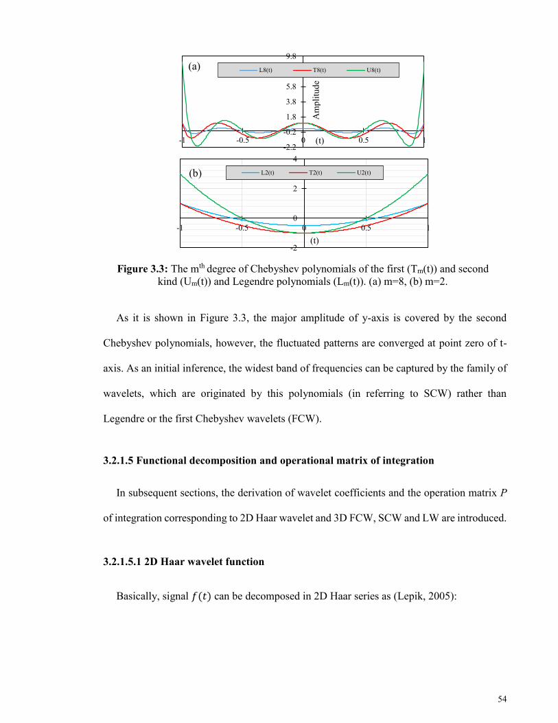
54

Figure 3.3: The mth degree of Chebyshev polynomials of the first (Tm(t)) and second

kind (Um(t)) and Legendre polynomials (Lm(t)). (a) m=8, (b) m=2.

As it is shown in Figure 3.3, the major amplitude of y-axis is covered by the second

Chebyshev polynomials, however, the fluctuated patterns are converged at point zero of t-

axis. As an initial inference, the widest band of frequencies can be captured by the family of

wavelets, which are originated by this polynomials (in referring to SCW) rather than

Legendre or the first Chebyshev wavelets (FCW).

3.2.1.5 Functional decomposition and operational matrix of integration

In subsequent sections, the derivation of wavelet coefficients and the operation matrix P

of integration corresponding to 2D Haar wavelet and 3D FCW, SCW and LW are introduced.

3.2.1.5.1 2D Haar wavelet function

Basically, signal 𝑓(𝑡) can be decomposed in 2D Haar series as (Lepik, 2005):

-2.2

-0.2

1.8

3.8

5.8

7.8

9.8

-1 -0.5 0 0.5 1

L8(t) T8(t) U8(t)

-2

0

2

4

-1 -0.5 0 0.5 1

L2(t) T2(t) U2(t)

(a)

(b)

(t)

(t)

Am

pli

tud

e

55

𝑓(𝑡) ≅∑𝑐𝑖ℎ𝑖(𝑡)

2𝑀

𝑖=0

(3.12)

Accordingly, Haar coefficients 𝑐𝑖 (𝑖 = 0, 1, 2, … ) are defined by:

𝑐𝑖 = 2𝑗∫ 𝑓(𝑡)1

0

ℎ𝑖(𝑡)𝑑𝑡 (3.13)

Hence, 𝐻2𝑀 is a square matrix (2𝑀 × 2𝑀), including the first 2𝑀 scales of Haar wavelet;

Haar coefficients are directly given as:

𝑐𝑖 = 𝑓(𝑡)𝐻2𝑀−1(𝑡) (3.14)

Equivalently, signal 𝑓(𝑡) may be rewritten as:

𝑓(𝑡) ≅ 𝑐2𝑀𝑇 𝐻2𝑀(𝑡) (3.15)

Subsequently, integration of 𝐻2𝑀 is obtained by Haar series with new square coefficient

matrix of integration 𝑃2𝑀 as (Lepik, 2005; Mahdavi and Shojaee, 2013):

∫ 𝐻2𝑀(𝑡)𝑑𝑡 ≈ 𝑃 𝐻2𝑀(𝑡)1

0

(3.16)

It should be noted that, local times are calculated relatively to the scale of wavelet as:

𝜏𝑙 =𝑙 − 0.5

2𝑀 , 𝑙 = 1, 2, … , 2𝑀 (3.17)

Finally, the local time divisions (𝜏𝑙), are adapted to the global domain. Assumption of 𝑑𝑡

as global time interval one may obtain (Lepik, 2005):

𝑡𝑙𝑡 = 𝑑𝑡(𝜏𝑙) + 𝑡𝑡 ⟹ 𝜏𝑙 =𝑡𝑡 − 𝑡𝑙𝑡𝑑𝑡

, 𝑙 = 1,2, … , 2𝑀 (3.18)

56

3.2.1.5.2 3D wavelet functions

Fundamentally, any quadratically-integrable function 𝑓(𝑡) may be expanded in terms of

FCW, SCW or Legendre wavelets (LW) for 𝑡 ∈ [0,1) as (Babolian and Fattahzadeh, 2007;

Razzaghi and Yousefi, 2001):

𝑓(𝑡) = ∑∑ 𝑐𝑛,𝑚𝜓𝑛,𝑚(𝑡)

∞

𝑚=0

∞

𝑛=1

(3.19)

Integrating both sides of Equation (3.19), and then multiplying by the components of

wavelets, corresponding wavelet coefficients are being obtained as follows (the orthogonality

is satisfied by employing the weight functions of 𝜔𝑛(𝑡)):

𝑐𝑛,𝑚 = (𝜓𝑛,𝑚(𝑡), 𝑓(𝑡), 𝜔𝑛(𝑡)) = ∫ 𝜔𝑛(𝑡)𝜓𝑛,𝑚(𝑡)1

0

𝑓(𝑡)𝑑𝑡 (3.20)

Subsequently, the function 𝑓(𝑡) can be decomposed by the truncated series of a wavelet’s

family as follows (Babolian and Fattahzadeh, 2007; Razzaghi and Yousefi, 2001):

𝑓(𝑡) ≅ ∑ ∑ 𝑐𝑛,𝑚𝜓𝑛,𝑚(𝑡) = 𝐶𝑇Ψ(𝑡)

𝑀−1

𝑚=0

2𝑘′−1

𝑛=1

(3.21)

where, 𝐶 denotes the coefficients vector of the relevant wavelets, i.e., FCW, SCW or

Legendre wavelets, and the corresponding wavelet function vector is designated by Ψ(𝑡) as:

𝐶 = [𝑐1, 𝑐2, 𝑐3, … , 𝑐2𝑘−1]2𝑘′−1𝑀×1𝑇

⟺ 𝑐𝑖

= [𝑐𝑖0, 𝑐𝑖1, 𝑐𝑖2, … , 𝑐𝑖,𝑀−1]𝑇 , 𝑖 = 1,2, … , 2𝑘

′−1

(3.22)

Ψ(𝑡) = [𝜓1, 𝜓2, 𝜓3, … , 𝜓2𝑘−1]2𝑘′−1𝑀×1 𝑇

⟺ 𝜓𝑖(𝑡)

= [𝜓𝑖0(𝑡), 𝜓𝑖1(𝑡), 𝜓𝑖2(𝑡), … , 𝜓𝑖,𝑀−1(𝑡)]𝑇

(3.23)

Eventually, a 2𝑘′−1𝑀 × 2𝑘

′−1𝑀-dimensional matrix of 𝜙𝑛,𝑚(𝑡) is formed as:

57

𝜙𝑛,𝑚(𝑡) = [Ψ(𝑡1) Ψ(𝑡2) … Ψ(𝑡𝑖)]2𝑘′−1𝑀×2𝑘′−1𝑀 (3.24)

The square matrix 𝜙𝑛,𝑚(𝑡) is populated with vectors of wavelet functions for a set of

discrete SM local points (𝑡𝑖, 𝑖 = 1, 2, 3, … , 2𝑘′−1𝑀).

It is assumed that the integration of Ψ(𝑡) can be obtained as (assumption of 𝑘′ = 2) :

∫ Ψ2𝑀(𝑡)1

0

𝑑𝑡 = 𝑃2𝑀Ψ(𝑡) (3.25)

In Equation (3.25), the subscripts of Ψ2𝑀 and 𝑃2𝑀indicate the dimensions of matrices.

Correspondingly, the 2𝑘′−1𝑀 × 2𝑘

′−1𝑀-dimension operational matrix P for FCW, SCW and

LW, which plays the underlying role in dealing with solution of differential equations is

derived as (𝑘′ = 2) (Babolian and Fattahzadeh, 2007; Razzaghi and Yousefi, 2000):

𝑃2𝑀 =1

2𝑘′

[ [𝐿]2𝑀

2×2𝑀2

[𝐹]2𝑀2×2𝑀2

𝐹 … 𝐹

[𝑂]2𝑀2×2𝑀2

[𝐿]2𝑀2×2𝑀2

𝐹 … 𝐹

𝑂 𝑂 ⋱ ⋱ ⋮⋮ ⋮ … ⋱ 𝐹𝑂 𝑂 … 𝑂 𝐿]

(3.26)

where, 2𝑀

2×2𝑀

2 square matrices F and L are given as follows ([𝑂] shows a zero matrix):

58

𝐹 =

[ 2 0 0 … 0 00 0 0 … 0 0𝑎1 0 0 … 0 00 0 0 ⋱ ⋮ ⋮⋮ ⋮ ⋮ ⋮ ⋱ ⋮𝑎2 0 … … 0 0]

,

𝐿 =

[ 1 𝑎6 𝑎9 𝑎12 … 0 0 0𝑎3 0 𝑎10 𝑎13 … 0 0 0𝑎4 𝑎7 0 𝑎14 … 0 0 0𝑎5 𝑎8 𝑎11 0 … ⋮ ⋮ ⋮⋮ ⋮ ⋮ ⋮ ⋱ ⋮ ⋮ ⋮⋮ ⋮ ⋮ ⋮ ⋮ ⋱ ⋮ ⋮𝑎15 0 0 … … 𝑎17 ⋱ 𝑎19𝑎16 0 0 … … 0 𝑎18 0 ]

(3.27)

Generally, it is inferred from Equations (3.26) and (3.27) that, there is a similar population

for components of P corresponding to considered wavelets. In details, particular coefficients

of 𝑎𝑖 are derived for FCW, SCW and LW, and tabulated in Table 3.1. It should be kept in

mind that 2𝑀

2 implies 2𝑘

′−1𝑀/2𝑘′−1. To calculate operation matrix of P for FCW, SCW and

LW, a backward algorithm of program coding is recommended. In other words, only the first

four rows and columns of P are being calculated, initially. At the second stage, the

components of P are being calculated and replaced from the last row and column 2𝑀

2 th until

computation of the 5th row and column. To clarify the expression of wavelets parameters of

FCW, SCW and LW, matrices of 𝜙4,4 and 𝑃4,4 are computed and shown in Table 3.2 for 𝑘′ =

2,2𝑀

2 = 2.

59

Table 3.1: Coefficients of 𝑎𝑖, defined in Equation (3.27) corresponding to FCW,

SCW and Legendre wavelets (2𝑀/2 = 𝑀).

𝒂𝒊 Legendre wavelet FCW SCW

𝑎1 0 −2√2 3⁄ 2/3

𝑎2 0 √2

2(1 − (−1)𝑀

𝑀−1 − (−1)𝑀−2

𝑀 − 2) |sin (

𝑀𝜋

2)|2

𝑀

𝑎3 −√3 3⁄ −√2 4⁄ −3/4

𝑎4 0 −√2 3⁄ 1/3

𝑎5 0 √2 4⁄ −1/4

𝑎6 1 √3⁄ 1 √2⁄ ½

𝑎7 −√5 (5√3)⁄ −1/2 −1/6

𝑎8 0 0 0

𝑎9 0 0 0

𝑎10 √3 (3√5)⁄ ¼ ¼

𝑎11 −√7 (7√5)⁄ −1/4 −1/8

𝑎12 0 0 0

𝑎13 0 0 0

𝑎14 √5 (5√7)⁄ 1/6 1/6

𝑎15 0 √2

2((−1)𝑀−3

𝑀 − 3−(−1)𝑀−1

𝑀 − 1) (−1)𝑀−2

1

𝑀 − 1

𝑎16 0 √2

2((−1)𝑀−2

𝑀 − 2−(−1)𝑀

𝑀) (−1)𝑀−1

1

𝑀

𝑎17 −

(2𝑀 − 3)1/2)

(2𝑀 − 3)(2𝑀 − 5)1/2

−1

2(𝑀 − 3) −

1

2(𝑀 − 1)

𝑎18 −

(2𝑀 − 1)1/2

(2𝑀 − 1)(2𝑀 − 3)1/2

−1

2(𝑀 − 2) −

1

2𝑀

𝑎19 (2𝑀 − 3)1/2

(2𝑀 − 3)(2𝑀 − 1)1/2

1

2(𝑀 − 1)

1

2(𝑀 − 1)

Note: FCW= first Chebyshev wavelet, SCW= second Chebyshev wavelet.

60

Furthermore, from the computational time point of view, Equation (3.27) and Table 3.1

demonstrate that the cost of computation of F and therefore P for LW (because of its scaled

weight functions) is less than either FCW or SCW, in which that, the whole arrays are zeros

(except for the first one). Significantly, the foregoing point is highlighted when higher

degrees of polynomials and scales of wavelets are employed. Basically, this is due to the

simple weight function 𝜔 = 1 of Legendre polynomials in contrast to the variable weight

functions of FCW and SCW. Accordingly, it will be shown later that the total CPU time for

solving especially large-scaled structures using free scales of LW is less than that of using

FCW or SCW. However, from accuracy point of view, variable weight functions of FCW

and SCW lead to less errors of end points of integration and resulting in more precise results

compared to the results obtained with LW.

3.2.1.6 Comparison of 2D and 3D wavelet functions

In this subsection, the characteristic of 2D Haar wavelet has been compared with FCW

known as a 3D wavelet function. It should be kept in mind that the characteristics of FCW,

SCW and LW are very close, so only FCW is considered here in order to reasonably compare

2D and 3D wavelets.

3.2.1.6.1 Inherent characteristics

As it was mentioned before, each particular scale of corresponding wavelet is constituted

by an improved wavelet function, related to the corresponding polynomial for 3D wavelets.

In other words, provided that scales of functions are being increased, basis functions will be

respectively developed.

61

Table 3.2: Corresponding components of wavelets 𝜙𝑖,𝑗 and 𝑃, calculated on four SM points for 2D Haar wavelet, 3D FCW, SCW and LW.

Column 𝒋 1 2 3 4 Row 𝒊 𝜙𝑖,𝑗 𝑃𝑖,𝑗 𝜙𝑖,𝑗 𝑃𝑖,𝑗 𝜙𝑖,𝑗 𝑃𝑖,𝑗 𝜙𝑖,𝑗 𝑃𝑖,𝑗

1 HA 1.0000 0.5000 1.0000 -0.2500 1.0000 -0.1250 1.0000 -0.1250

FCW 1.1284 0.2500 1.1284 0.1768 0 0.5000 0 0 SCW 1.5958 0.2500 1.5958 0.1250 0 0.5000 0 0 LW 1.4142 0.2500 1.4142 0.1442 0 0.5000 0 0

2 HA 1.0000 0.2500 1.0000 0 -1.0000 -0.1250 -1.0000

FCW -0.7979 -0.0884 0.7979 0 0 0 0 0 SCW -1.5958 -0.1875 1.5958 0 0 0 0 0 LW -1.2247 -0.1442 1.2247 0 0 0 0 0

3 HA 1.0000 0.0625 -1.0000 0.0625 0 0 0 0.1250

FCW 0 0 0 0 1.1284 0.2500 1.1284 0.1768 SCW 0 0 0 0 1.5958 0.2500 1.5958 0.1250 LW 0 0 0 0 1.4142 0.2500 1.4142 0.1442

4 HA 0 0.0625 0 -0.0625 1.0000 0 -1.0000 0

FCW 0 0 0 0 -0.7979 -0.0884 0.7979 0 SCW 0 0 0 0 -1.5958 -0.1875 1.5958 0 LW 0 0 0 0 -1.2247 -0.1442 1.2247 0

Note: HA=Haar wavelet, FCW= first Chebyshev wavelet, SCW= second Chebyshev wavelet, LW= Legendre wavelet.

62

Figure 3.4 shows the first 8 scales of Haar and Chebyshev families. It can be seen from

Figure 3.4(a) that, for the 8th scale of Haar family, the simple basis function has been just

compressed and afterward has been delayed from the first position. In contrast, Figure 3.4(b)

shows the broad-band frequency function of the 8th scale of Chebyshev that will be moved

along the time axis.

Figure 3.4: Comparison of the first 8th scales of wavelet functions, (a) 2D Haar family,

(b) 3D Chebyshev polynomial.

Additionally, the shortcoming of Haar wavelet is shown in Figure 3.4(a) at the point of

0.5, which the continuity is not satisfied at this point. According to a mathematical rule, the

second derivation will not exist at the point of 0.5. As a result, it is just possible to implement

an indirect formulation for solving the second-ordered differential equation of motion.

Consequently, as will be shown in this chapter, large values of errors have been computed

by using free-scaled Haar wavelet functions through the direct practice of the proposed

scheme. However, with far lesser CPU time taken (analysis cost) that will be discussed later.

3.2.1.6.2 Functional approximation

Fundamentally, optimum structural dynamics can be achieved through a wavelet-based

approach involving two parts of numerical analysis. Firstly, the external loading is accurately

approximated according to its frequency contents simultaneously with numerical time

-1

-0.5

0

0.5

1

-1 -0.75 -0.5 -0.25 0 0.25 0.5 0.75 1

1

1

1

1

1

1

1

1

1

1

1 1

1

1

1 1

h0

h1

h2

h3

h4

h5

h6

h7

63

integration procedure. Secondly, differential equations are accurately converted to an

algebraic system by wavelet functions on a corresponding set of collocation points, even with

a long time step. Consequently, it is inferred that accuracy of results are directly dependent

on accurate approximation of equations.

Figure 3.5: Approximation of F(t) and wavelet coefficients for the first 8th scale of (a)

FCW, (b) Haar wavelet, at the first second of F(t) and 𝝎=8 rad/sec (CH_CW=

coefficients of FCW, HA_CW= coefficients of Haar wavelet, App. of F(t)_CH/HA=

approximation of F(t) using Chebyshev/Haar wavelet).


FCW, (b) Haar wavelet, for the first second of F(t) and 𝝎=15 rad/sec (CH_CW=

coefficients of FCW, HA_CW= coefficients of Haar wavelet, App. of F(t)_CH/HA=

approximation of F(t) using Chebyshev/Haar wavelet).

In order to evaluate the accuracy of approximation by using wavelet functions, the first

8th scale of Haar wavelet and FCW are exemplified for three different frequency-content

-1.5

-1

-0.5

0

0.5

1

1.5

0 0.2 0.4 0.6 0.8 1

CH_CW F(t) App. Of F(t)_CH -1.5

-1

-0.5

0

0.5

1

1.5

0 0.2 0.4 0.6 0.8 1

HA_CW F(t) App. Of F(t)_HA

-1.5

-1

-0.5

0

0.5

1

1.5

0 0.2 0.4 0.6 0.8 1

CH_CW F(t) App. Of F(t)_CH-1.5

-1

-0.5

0

0.5

1

1.5

0 0.2 0.4 0.6 0.8 1

HA_CW F(t)

App. Of F(t)_HA

Time(sec) Time(sec)

(a) (b)

Time(sec) Time(sec)

64

signals, accordingly. For this purpose, a sinusoidal function of 𝐹(𝑡)= sin (𝜔𝑡) is examined

for 𝜔 equal to 8, 15 and 500 rad/sec, at the first second of excitation, respectively.

Figure 3.5 shows that the accuracy of approximation for 𝜔=8 rad/sec through the

calculated coefficients of FCW (designated by CH_CW) is more than Haar wavelet. The

corresponding function is also examined to be almost accurate with Haar wavelet

(coefficients of Haar wavelet are designated by HA_CW). Additionally, Figure 3.6 illustrates

the capability of 8th scale of 3D FCW which is a low scale of this wavelet, compared with

acceptable decomposition by using the same-scaled 2D Haar wavelet. Despite the

undesirable approximation of Haar wavelet for 𝜔=15 rad/sec, from its optimization point of

view the results could be interpreted as acceptable approximation. Finally, Figure 3.7(b)

shows the rejected results through the 8th scale of Haar wavelet, encountering with a high

frequency-content signal with 𝜔=500 rad/sec. It is clearly shown in the figure that the 128th

scale of Haar wavelet gave sufficient accuracy of approximation. However, with a very long

computation time involved. Overall, figures demonstrate the efficiency of low-scaled FCW;

although, for the case of 𝝎=500 rad/sec higher scales shall be utilized in order to obtain

accurate results.

65


FCW, (b) Haar wavelet, for the first second of F(t) and 𝝎=500 rad/sec (CH_CW=

coefficients of FCW, HA_CW= coefficients of Haar wavelet, App. of F(t)_CH=

approximation of F(t) using FCW, App. of F(t)_HA(2M8/128)= approximation of F(t)

using the first 8/128th scale of Haar wavelet).

3.2.2 The proposed method for dynamic analysis of SDOF structures

Generally, the linear dynamic equilibrium (ordinary differential equation) governing the

SDOF system of mass (𝑚), damping (𝑐) and stiffness (𝑘) is expressed as follows (Hughes,

2012):

(𝑚)�̈�(𝑡) + (𝑐)�̇�(𝑡) + (𝑘)𝑢(𝑡) = 𝐹(𝑡) (3.28)

where, �̈�(𝑡), �̇�(𝑡) and 𝑢(𝑡) denote acceleration, velocity and displacement vectors of

response to the external dynamic load of 𝐹(𝑡), respectively. Using Equation (3.12) for 2D

wavelets or Equation (3.19) for 3D wavelets, acceleration vectors can be decomposed on 2𝑀

adaptive (SM) points of analysis corresponding to Haar wavelet, FCW, SCW or LW as:

-1.5

-1

-0.5

0

0.5

1

1.5

0 0.2 0.4 0.6 0.8 1

CH_CW F(t) App. Of F(t)_CH -1.5

-1

-0.5

0

0.5

1

1.5

0 0.2 0.4 0.6 0.8 1

HA_CW

F(t)

App. Of F(t)_HA(2M8)

App. Of F(t)_HA(2M128)

(b)

Time(sec) Time(sec)

(a)

66

�̈�(𝑡) ≅ ∑ ∑ 𝑐𝑛,𝑚𝜓𝑛,𝑚(𝑡) = 𝐶𝑇Ψ(𝑡)

𝑀−1

𝑚=0

2𝑘′−1

𝑛=1

(3.29)

In addition, Ψ(𝑡) represents the operation vector of FCW, SCW or LW, which can be

replaced by ℎ(𝑡) for Haar wavelet. Subsequently, using Equation (3.25) the first and second

orders of integration vectors, namely, velocity and displacement vectors are approximated as

(let �̇�𝑛 = 𝑣𝑛initial velocities and 𝑢𝑛 initial displacements):

�̇�(𝑡) = 𝐶𝑇𝑃Ψ(𝑡) + 𝑣𝑛 (3.30)

𝑢(𝑡) = 𝐶𝑇𝑃2Ψ(𝑡) + 𝑢𝑛 (3.31)

It is to be noted that, 𝑢𝑛and 𝑣𝑛are a constant initial value in global time interval of 𝑑𝑡 =

𝑡𝑖+1 − 𝑡𝑖. Furthermore, the numerical algebraic equation in Equations (3.30) or (3.31) is

satisfied by decomposition of unity for 2𝑀 adaptive points of FCW, SCW and LW as

follows:

1 ≅ 𝐼∗Ψ(𝑡) ≅ 𝐷[11,1, 0,0, … , 11,𝑀+1, 0,0, … ]Ψ(𝑡) (3.32)

where, D=√𝜋 4⁄ , √𝜋 8⁄ and √1 2⁄ for FCW, SCW and LW, respectively.

It should be emphasized that, the size of vector in 𝐼∗ is 1 × 2𝑀. For FCW, SCW and LW,

the first component and (2𝑀/2)+1 are one. Similarly, for Haar wavelet it is also determined

as:

1 ≅ 𝐼∗ℎ(𝑡) ≅ [11,1, 0,0, … ,0,0,0, … , 01,2𝑀]ℎ(𝑡) (3.33)

Therefore, the constant values of initial displacement and velocity (calculated from

previous step) are approximated by corresponding wavelets as (designated by 𝑆2𝑇Ψ(𝑡) and

𝑆1𝑇Ψ(𝑡)):

67

𝑆1𝑇Ψ(𝑡) = 𝑣𝑛 × 1 ≅ 𝑣𝑛𝐼

∗Ψ(𝑡)

≅ 𝑣𝑛𝐷[11,1, 0,0, … , 11,𝑀+1, 0,0, … ]Ψ(𝑡) (3.34)

𝑆2𝑇Ψ(𝑡) = 𝑢𝑛 × 1 ≅ 𝑢𝑛𝐼

∗Ψ(𝑡)

≅ 𝑢𝑛𝐷[11,1, 0,0, … , 11,𝑀+1, 0,0, … ]Ψ(𝑡)

(3.35)

Quantities of velocity and displacement vectors are numerically developed on 2𝑀 points

by substituting Equations (3.34) and (3.35) into Equations (3.30) and (3.31) as follows:

�̇�(𝑡) = 𝐶𝑇𝑃Ψ(𝑡) + 𝑆1𝑇Ψ(𝑡) (3.36)

𝑢(𝑡) = 𝐶𝑇𝑃2Ψ(𝑡) + 𝑆1𝑇𝑃Ψ(𝑡) + 𝑆2

𝑇Ψ(𝑡) (3.37)

On the other hand, the external excitation 𝐹(𝑡), which most of the time (in actual cases)

is a wide-band frequency content signal, can be decomposed with Haar wavelet, FCW, SCW

or LW as follows:

𝐹(𝑡) = 𝑓𝑇Ψ(𝑡) (3.38)

The applied signal known as external loading of 𝐹(𝑡) may be constructed by several sets

of discrete 1× 2𝑘′−1𝑀-dimensional vectors corresponding to 2𝑀 points of global time. Thus,

coefficients vector of 𝑓𝑇is obtained for each separate vector as follows:

𝑓1×2𝑘

′−1𝑀

𝑇 = 𝐹1×2𝑘

′−1𝑀𝜙(2𝑘

′−1𝑀)×(2𝑘′−1𝑀)

⁄ (3.39)

Substituting Equations (3.36), (3.37) and (3.39) into Equation (3.28), the dynamic

equilibrium is numerically developed as:

(𝑚)[𝐶𝑇Ψ(𝑡)] + (𝑐)𝑑𝑡[𝐶𝑇𝑃Ψ(𝑡) + 𝑆1

𝑇Ψ(𝑡)]

+ (𝑘)𝑑𝑡2[𝐶𝑇𝑃2Ψ(𝑡) + 𝑆1

𝑇𝑃Ψ(𝑡) + 𝑆2𝑇Ψ(𝑡)]

= 𝑑𝑡2𝑓𝑇Ψ(𝑡)

(3.40)

68

In addition, quantities of the dynamic system are transformed from the alternative domain

of analysis (2𝑀 local times of wavelets) into the setting domain (2𝑀 global times) by

multiplying 𝑑𝑡 to each operation of derivative. This implementation makes the proposed

scheme applicable for analysis of time domains larger than unity. Eventually, Ψ(𝑡) is omitted

from the both sides of Equation (3.40), and the algebraic system is improved as follows:

(𝑚)[𝐶𝑇] + (𝑐)𝑑𝑡[𝐶𝑇𝑃 + 𝑆1

𝑇] + (𝑘)𝑑𝑡2[𝐶𝑇𝑃2 + 𝑆1

𝑇𝑃 + 𝑆2𝑇]

= 𝑓𝑇𝑑𝑡2

(3.41)

Calculating coefficient vectors of wavelets (𝐶𝑇for Haar wavelet, FCW, SCW or LW) from

Equation (3.41) and substituting into Equations (3.30) and (3.31), quantities of displacement

and velocity vectors are computed corresponding to 2𝑀 global points for each wavelet

function.

In theory, it is clearly distinguishable that vibration equations are being approximated

undesirably with 2D Haar wavelets, because of its inherent simple shape function. However,

in practice to gain the optimal time vibration analysis by taking into consideration the least

computation time involved, this simple wavelet can be utilized for initial predictions.

3.2.3 The proposed method for dynamic analysis of MDOF structures

In structural dynamic problems, the constant values of mass (𝑚), damping (𝑐) and stiffness

(𝑘) relevant to a SDOF system are replaced by matrices of mass [𝑀]𝑑×𝑑, damping [𝐶𝑑]𝑑×𝑑

and stiffness [𝐾]𝑑×𝑑 corresponding to the considered MDOF system with 𝑑 degrees of

freedom, subjected to the vector of applied forces of {𝐹𝑡}. Hence, the dynamic equilibrium

is developed as:

[𝑀]𝑑×𝑑�̈�𝑑×2𝑀𝑡 + [𝐶𝑑]𝑑×𝑑�̇�𝑑×2𝑀

𝑡 + [𝐾]𝑑×𝑑𝑈𝑑×2𝑀𝑡 = {𝐹𝑡}𝑑×2𝑀 (3.42)

69

The subscripts of �̈�𝑑×2𝑀𝑡 , �̇�𝑑×2𝑀

𝑡 and 𝑈𝑑×2𝑀𝑡 denote 𝑑 × 2𝑀-dimensional acceleration,

velocity and displacement vectors related to 2𝑀 adaptive collocation points of global time

corresponding to each degree of freedom (DOF), respectively. Accordingly, the expansion

of Equation (3.29) is employed for each DOF. Initial conditions corresponding to each DOF

is also approximated with wavelet functions using Equations (3.34) and (3.35). Moreover,

nodal forces are also decomposed by using Equation (3.39) on each DOF. Eventually, the

convertor of local times to global times is executed by multiplying 𝑑𝑡, and therefore Equation

(3.42) is numerically developed as:

[𝑀] [𝐶1𝑇Ψ(𝑡)⋮

𝐶𝑑𝑇Ψ(𝑡)

] + [𝐶𝑑]𝑑𝑡 [𝐶1𝑇𝑃Ψ(𝑡) + 𝑆1−1

𝑇 Ψ(𝑡)⋮

𝐶𝑑𝑇𝑃Ψ(𝑡) + 𝑆1−𝑑

𝑇 Ψ(𝑡)] +

[𝐾]𝑑𝑡2 [𝐶1𝑇𝑃2Ψ(𝑡) + 𝑆1−1

𝑇 𝑃Ψ(𝑡) + 𝑆2−1𝑇 Ψ(𝑡)

⋮𝐶𝑑𝑇𝑃2Ψ(𝑡) + 𝑆1−𝑑

𝑇 𝑃Ψ(𝑡) + 𝑆2−𝑑𝑇 Ψ(𝑡)

]=𝑑𝑡2 [𝑓1𝑇Ψ(𝑡)⋮

𝑓𝑑𝑇Ψ(𝑡)

]

(3.43)

Eliminating Ψ(𝑡) from the both sides, Equation (3.43) is represented as a vector for each

row corresponding to each DOF (1-𝑑) and 𝑗 = 1,2, … , 𝑑 we have:

∑[𝑀]𝑗𝑖𝐶𝑖

𝑇

𝑑

𝑖=1

+ 𝑑𝑡∑[𝐶𝑑]𝑗𝑖(𝐶𝑖𝑇𝑃 + 𝑆1−𝑖

𝑇 ) + 𝑑𝑡2

𝑑

𝑖=1

∑[𝐾]𝑗𝑖(𝐶𝑖𝑇𝑃2

𝑑

𝑖=1

+ 𝑆1−𝑖𝑇 𝑃 + 𝑆2−𝑖

𝑇 ) = 𝑑𝑡2𝑓𝑗

𝑇

(3.44)

Assumption of 𝐼2𝑀×2𝑀 as an identity matrix, Equation (3.44) is simplified as follows:

𝐶𝑖𝑇([𝑀]𝑗𝑖𝐼 + 𝑑𝑡[𝐶𝑑]𝑗𝑖𝑃 + 𝑑𝑡

2[𝐾]𝑗𝑖𝑃2)

= 𝑑𝑡2𝑓𝑗

𝑇

−∑[𝑑𝑡[𝐶𝑑]𝑗𝑖𝑆1−𝑖𝑇 + 𝑑𝑡

2[𝐾]𝑗𝑖(𝑆1−𝑖𝑇 𝑃 + 𝑆2−𝑖

𝑇 )]

𝑑

𝑖=1

(3.45)

70

Calculating coefficients vectors of wavelet 𝐶𝑖𝑇 (𝑖 = 1,2, … , 𝑑) for each DOF in Equation

(3.45), and therefore using Equations (3.31) and (3.30), velocity and displacement vectors

are obtained corresponding to each DOF.

Note that in large-scaled linear systems, due to the sequence in the node numbering, the

coefficient matrix on the left side of Equation (3.45) is nearly singular. Thus, it is

recommended to solve the coefficients of wavelet in the above algebraic system using

singular value decomposition (SVD) method. However, for many applications, simple

decomposition techniques are applicable, i.e., the Choleski factorization method. The step-

by-step algorithm of the proposed method is tabulated in Table 3.3.

To achieve an optimum analysis, it is recommended to determine 𝑑𝑡 = ∆𝑡 ≤ 2 × 𝑇𝑚𝑖𝑛

(𝑇𝑚𝑖𝑛= minimum period of system), as long as the stability of results is satisfied. For this

reason, the stability analysis is essential for the proposed method. The statement of optimum

analysis refers to an accurate analysis with lesser computation time involved, and therefore

lesser amounts of storage capacity (namely, the optimum cost of analysis). It is to be noted

that, the sampling rate of external loading shall be considered as another important criteria to

specify 2𝑀 and 𝑑𝑡.

71

Table 3.3: Step-by-step algorithm to calculate the response of MDOF systems using the

proposed method for Haar wavelet, FCW, SCW and LW.

A. Initial calculations:

(1) Form stiffness matrix [K], damping matrix [Cd] and mass matrix [M] of the system.

(2) Specify wavelet basis function, number of adaptive collocation points 2M, the

considered order of wavelet 𝒎=(2M/2)-1.

(3) Select an appropriate time step 𝒅𝒕. (4) Specify vectors of applied forces on each DOF of system, in each 𝒅𝒕 corresponding to

collocation points.

(5) Form coefficients wavelet matrix corresponding to collocation points for free-scaled

orders of wavelet function 𝝓(𝒕). (6) Form operation matrix of integration corresponding to collocation points for each

particular wavelet function 𝑷.

(7) Calculate square operational matrix 𝑷𝟐.

(8) Approximate unity, with related coefficient of wavelets.

- D=√𝜋 4⁄ , √𝜋 8⁄ and √1 2⁄ for FCW, SCW and LW,

respectively.

(9) Initialize 𝒖𝟎 and 𝒗𝟎 as initial displacement and velocity vectors.

(10) Form 𝟐𝑴× 𝟐𝑴 identity matrix of 𝑰.

B. For each time step:

(1) Form initial vectors for velocity and displacement of 𝑺𝟏𝑻 and 𝑺𝟐

𝑻.

(2) Calculate 𝒖𝒏𝟎 and 𝒗𝒏𝟎using:

𝑣𝑛0 = 𝑆1𝑇Ψ(𝑡)

𝑢𝑛0 = 𝑆2𝑇Ψ(𝑡)

(3) Calculate vectors of unknown coefficients of 𝑪𝒊𝑻 for each DOF (i=1,2,…,d).

(4) For each DOF calculate displacement, velocity and acceleration vectors,

simultaneously by:

𝑢(𝑡) = 𝐶𝑇𝑃2Ψ(𝑡) + 𝑢𝑛0

�̇�(𝑡) = 𝐶𝑇𝑃Ψ(𝑡) + 𝑣𝑛0

�̈�(𝑡) = 𝐶𝑇Ψ(𝑡)

72

3.3 Stability analysis of the wavelet-based method

As was shown in previous sections, the robustness of the proposed method is revealed

while the quantities of the dynamic system (i.e., displacements, velocities and accelerations)

have been transferred from 𝑡th step to the (𝑡+𝑑𝑡)th step using a set of compatible collocation

(SM) points. Subsequently, details (e.g., frequency contents) of either dynamic responses

(left side of Equation (3.42)) or externally applied loadings (right side of Equation (3.42))

are precisely captured by adaptive collocation SM points. Consequently, it provides the

possibility of using longer time intervals of 𝑑𝑡. However, different sets of collocation points

may be utilized, relating to the diverse details of considered problem. For this reason, the

stability analysis of calculated results using the proposed scheme is concerned in this section

for the least number of 2𝑀=2 collocation points. The relationship between dynamic

quantities of the current state (�̂�𝑡+∆𝑡) and the previous state (�̂�𝑡) is presented as (Bathe, 2006;

Bathe and Wilson, 1973):

{�̂�𝑡+∆𝑡} = [𝐴]{�̂�𝑡} + [𝐿′]{𝑓𝑡+𝜐∆𝑡} (3.46)

where, 𝐿′ and 𝐴 denote the load operator and amplification matrix, respectively. 𝑓𝑡+𝜐

indicates external loads which are related to the current quantities (𝜐 = 0,1,2,…). Note that,

𝑓𝑡+𝜐 , 𝐿′ and 𝐴 can be obtained for any numerical integration method, i.e., explicit or implicit

schemes. For the purpose of stability analysis, dynamic equilibrium of a SDOF structure in

Equation (3.28) is considered when there is no external load (𝑓𝑡+𝜐∆𝑡) applied. Firstly, the

representation of Equation (3.28) is changed from damping (𝑐) and stiffness (𝑘) to the

damping ratio (𝜉) and natural frequency (𝜔) as follows:

73

�̈�𝑡(𝑡) + 2𝜉𝜔�̇�𝑡(𝑡) + 𝜔2𝑢𝑡(𝑡) =

𝐹(𝑡)

(𝑚) (3.47)

The subscript �̈�𝑡(𝑡) indicates the relevant quantities at the current state of 𝑡. To calculate

amplification matrix of 𝐴, relatively with terms of accelerations, the third ordered derivative

of displacement with respect to time �⃛�(𝑡) is approximated by using the expansion of Equation

(3.29). Employing the operation matrix of integration P, quantities of acceleration, velocity

and displacement are obtained as follows:

�⃛�𝑡(𝑡) = 𝐶𝑇Ψ(𝑡)

�̈�𝑡(𝑡) = 𝑑𝑡. 𝐶𝑇𝑃Ψ(𝑡) + �̈�𝑡−Δ𝑡

�̇�𝑡(𝑡) = 𝑑𝑡2. 𝐶𝑇𝑃2Ψ(𝑡) + �̇�𝑡−Δ𝑡

𝑢𝑡(𝑡) = 𝑑𝑡3. 𝐶𝑇𝑃3Ψ(𝑡) + 𝑢𝑡−Δ𝑡

(3.48)

where, initial accelerations �̈�𝑡−Δ𝑡 is also approximated as:

𝑆𝑜𝑇Ψ(𝑡) = �̈�𝑡−Δ𝑡 × 1 ≅ �̈�𝑡−Δ𝑡. 𝐼

∗Ψ(𝑡)

≅ �̈�𝑡−Δ𝑡. 𝐷[11,1, 0,0, … , 11,𝑀+1, 0,0, … ]Ψ(𝑡) (3.49)

where, 𝐷 is defined in Equations (3.33) and (3.34) for FCW, SCW and LW. The subscripts

of �̈�𝑡−Δ𝑡, �̇�𝑡−Δ𝑡 and 𝑢𝑡−Δ𝑡 denote acceleration, velocity and displacement which were

calculated at the previous state, respectively. In addition, initial quantities in Equation (3.49)

are numerically developed by Equations (3.33) and (3.34) corresponding to Haar wavelet,

FCW, SCW and LW, substituting in Equation (3.47), after omitting Ψ(𝑡) yields:

𝐶𝑇𝑃 + 𝑆𝑜𝑇 + 2𝜉𝜔Δ𝑡[𝐶𝑇𝑃2 + 𝑆𝑜

𝑇𝑃 + 𝑆1𝑇]

+ 𝜔2Δ𝑡2[𝐶𝑇𝑃3 + 𝑆𝑜𝑇𝑃2 + 𝑆1

𝑇𝑃 + 𝑆2𝑇] = 0

(3.50)

74

After a set of algebraic simplification, coefficients vector of 𝐶𝑇is derived from Equation

(3.50). Substituting 𝐶𝑇in Equation (3.46), the amplification matrix of 𝐴 which shows the

relationship between quantities of the current state (i.e., �̈�𝑡(𝑡)) and the previous state (i.e.,

�̈�𝑡−Δ𝑡) is derived for FCW, SCW or LW (for corresponding 𝜙(𝑡), 𝐷 and 𝐼∗) as:

[

�⃛�𝑡�̈�𝑡�̇�𝑡𝑢𝑡

] = [

0 𝑎𝜙(𝑡) 𝑏𝜙(𝑡) 𝑐𝜙(𝑡)0 𝑑𝜙(𝑡) 𝑒𝜙(𝑡) 𝑓𝜙(𝑡)

0 𝑔𝜙(𝑡) 𝑖𝜙(𝑡) 𝑗𝜙(𝑡)0 𝑞𝜙(𝑡) 𝑟𝜙(𝑡) 𝑧𝜙(𝑡)

] [

�⃛�𝑡−Δ𝑡�̈�𝑡−Δ𝑡�̇�𝑡−Δ𝑡𝑢𝑡−Δ𝑡

] (3.51)

where;

𝑎 = 𝜅 𝜇−1 , 𝑏 = 휂 𝜇−1 , 𝑐 = Υ 𝜇−1

𝑑 = 𝐼∗ + 𝜅 𝜇−1𝑃 , 𝑒 = 휂 𝜇−1𝑃 , 𝑓 = Υ 𝜇−1𝑃

𝑔 = 𝐼∗𝑃 + 𝜅 𝜇−1𝑃2 , 𝑖 = 𝐼∗ + 휂 𝜇−1𝑃2 , 𝑗 = Υ 𝜇−1𝑃2

𝑞 = 𝐼∗𝑃2 + 𝜅 𝜇−1𝑃3 , 𝑟 = 𝐼∗𝑃 + 휂 𝜇−1𝑃3 ,

𝑧 = 𝐼∗ + Υ 𝜇−1𝑃3

(3.52)

where;

𝜅 = − 𝐼∗ − 2𝜉𝜔(Δ𝑡) 𝐼∗𝑃 − 𝜔2(Δ𝑡)2𝐼∗ 𝑃2

휂 = −2𝜉𝜔(Δ𝑡) 𝐼∗ −𝜔2(Δ𝑡)2 𝐼∗𝑃

Υ = −𝜔2(Δ𝑡)2 𝐼∗

𝜇 = 𝑃 + 2𝜉𝜔(Δ𝑡) 𝑃2 + 𝜔2(Δ𝑡)2 𝑃3

(3.53)

where, 𝜇 is a 2𝑀 × 2𝑀-dimensional matrix; 𝜅, 휂 and Υ are 1 × 2𝑀-dimensional vectors.

Accordingly, the amplification matrix of 𝐴 is decomposed into its eigen vectors [Φ] and

diagonal eigenvalue matrix of [λ] by 𝐴 = [Φ][𝜆][Φ]−1, and therefore stability of the

proposed method is satisfied provided that the maximum norm of elements [𝜆], namely,

spectral radius being less than unity as follows (Bathe, 2006; Bathe and Wilson, 1973):

𝜌(𝐴) = max (‖𝜆1‖, ‖𝜆2‖, ‖𝜆3‖,… ) ≤ 1 (3.54)

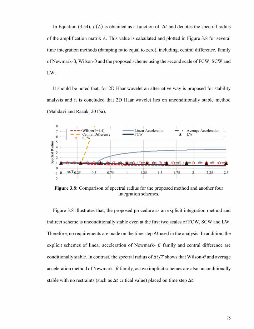
75

In Equation (3.54), 𝜌(𝐴) is obtained as a function of Δ𝑡 and denotes the spectral radius

of the amplification matrix 𝐴. This value is calculated and plotted in Figure 3.8 for several

time integration methods (damping ratio equal to zero), including, central difference, family

of Newmark-β, Wilson-θ and the proposed scheme using the second scale of FCW, SCW and

LW.

It should be noted that, for 2D Haar wavelet an alternative way is proposed for stability

analysis and it is concluded that 2D Haar wavelet lies on unconditionally stable method

(Mahdavi and Razak, 2015a).

Figure 3.8: Comparison of spectral radius for the proposed method and another four

integration schemes.

Figure 3.8 illustrates that, the proposed procedure as an explicit integration method and

indirect scheme is unconditionally stable even at the first two scales of FCW, SCW and LW.

Therefore, no requirements are made on the time step ∆𝑡 used in the analysis. In addition, the

explicit schemes of linear acceleration of Newmark- 𝛽 family and central difference are

conditionally stable. In contrast, the spectral radius of Δ𝑡/𝑇 shows that Wilson-휃 and average

acceleration method of Newmark- 𝛽 family, as two implicit schemes are also unconditionally

stable with no restraints (such as ∆𝑡 critical value) placed on time step ∆𝑡.

-2

-1

0

1

2

3

4

5

6

7

8

0 0.25 0.5 0.75 1 1.25 1.5 1.75 2 2.25 2.5

Sp

ectr

al R

adiu

s

∆t/T

Wilson(θ=1.4) Linear Acceleration Average AccelerationCentral Difference FCW LWSCW

76

Figure 3.9: Comparison of spectral radius calculated for the second scale of FCW,

SCW and LW.

3.4 Accuracy analysis of the wavelet-based scheme

In general, errors are inherent characteristic of numerical approaches (Bathe, 2006). Thus,

in the following section, accuracy of the proposed method is investigated corresponding to

free scales of Haar wavelet, FCW, SCW and LW. For this purpose, three operations are

considered, i.e., implementation of the first and second operation of integration and accuracy

analysis of functional approximation.

3.4.1 First ordered operation of integration

In order to investigate the accuracy of results calculated after the first ordered operation

of integration, the first-ordered ordinary differential equation of 0.25�̇�(𝑡) + 𝑢(𝑡) =

1, 𝑢(0) = 1 with the analytical solution of 𝑢(𝑡) = 1 − 𝑒(−4𝑡) is considered. For an accurate

comparison, the measurement of percentile total average relative errors (PTARE) is

compared, when free scales of FCW, SCW and LW are employed. Assumption of ∝̂ for the

measurement of exact results and �̂� related to the responses calculated by each numerical

integration scheme (relative errors corresponding to each �̂� = time increments), PTARE is

obtained as follows:

0.70

0 1 2 3 4 5 6 7 8

Sp

ectr

alR

adiu

s

∆t/T

FCW LW SCW

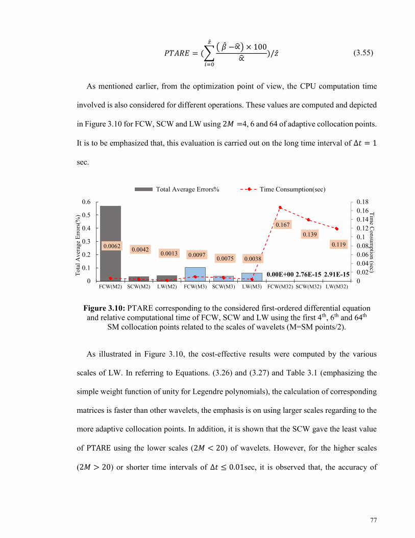
77

𝑃𝑇𝐴𝑅𝐸 = (∑( �̂� −∝̂) × 100

∝̂

�̂�

𝑖=0

)/�̂� (3.55)

As mentioned earlier, from the optimization point of view, the CPU computation time

involved is also considered for different operations. These values are computed and depicted

in Figure 3.10 for FCW, SCW and LW using 2𝑀 =4, 6 and 64 of adaptive collocation points.

It is to be emphasized that, this evaluation is carried out on the long time interval of ∆𝑡 = 1

sec.

Figure 3.10: PTARE corresponding to the considered first-ordered differential equation

and relative computational time of FCW, SCW and LW using the first 4th, 6th and 64th

SM collocation points related to the scales of wavelets (M=SM points/2).

As illustrated in Figure 3.10, the cost-effective results were computed by the various

scales of LW. In referring to Equations. (3.26) and (3.27) and Table 3.1 (emphasizing the

simple weight function of unity for Legendre polynomials), the calculation of corresponding

matrices is faster than other wavelets, the emphasis is on using larger scales regarding to the

more adaptive collocation points. In addition, it is shown that the SCW gave the least value

of PTARE using the lower scales (2𝑀 < 20) of wavelets. However, for the higher scales

(2𝑀 > 20) or shorter time intervals of ∆𝑡 ≤ 0.01sec, it is observed that, the accuracy of

0.00E+00 2.76E-15 2.91E-15

0.00620.0042

0.0013 0.00970.0075 0.0038

0.167

0.139

0.119

0

0.02

0.04

0.06

0.08

0.1

0.12

0.14

0.16

0.18

0

0.1

0.2

0.3

0.4

0.5

0.6

FCW(M2) SCW(M2) LW(M2) FCW(M3) SCW(M3) LW(M3) FCW(M32) SCW(M32) LW(M32)

Total Average Errors% Time Consumption(sec)

To

tal

Av

erag

e E

rro

rs(%

)

Tim

e Co

nsu

mptio

n (sec)

78

FCW is better than SCW or LW. It should be noted that, at current assessment of accuracy

there is no consideration on the frequency components.

3.4.2 Second ordered operation of integration

In order to evaluate the accuracy of results employing the second-ordered operation of

integration, the linear and second-ordered ordinary differential equation governing a free

vibrating and undamped SDOF system with constant circular frequency of 𝜔 is considered

as:

�̈�(𝑡) + 𝜔2𝑢(𝑡) = 0 (3.56)

Analytically, with the initial conditions of �̈�0= −𝜔2, �̇�0 = 0 and 𝑢0 = 1, the closed-

form solution of Equation (3.56) is 𝑢(𝑡) = cos (𝜔𝑡). In addition, the natural undamped period

is obtained by 𝑇0 = 2𝜋/𝜔 sec. The considered SDOF system has a cyclic response with a

constant maximum amplitude of |𝑢(𝑡)|𝑚𝑎𝑥 = (𝑢02 + (�̇�0 𝜔⁄ )2)0.5. In general, the accuracy

analysis can be achieved by presenting two kinds of error measurement; (a) period elongation

PE and (b) amplitude decay AD. Accordingly, PE measures the extension in the time interval

it takes to complete each cycle of harmonic response (Figure 3.11). While, AD is the absolute

error of the calculated results for 𝑢 (displacement) by each numerical scheme (shown in

Figure 3.11). However, AD is also known as algorithmic damping which is obtained by 𝐴𝐷 =

2𝜋𝜉. Eventually, the explained SDOF system is solved using some of the common numerical

integration procedures such as average acceleration (AA), linear acceleration (LA) from

Newmark-β family, central difference and Wilson-θ. Accordingly, two kinds of error are

measured, and therefore compared with the responses calculated using the proposed method

of FCW, SCW and LW on 2𝑀 = 2, SM points (in referring to the scale of the wavelets). The

PE and AD measurements are plotted in Figure 3.11 for the variations of Δ𝑡/𝑇0.

79

Figure 3.11: Error measurment. (a) Period elongation (PE=(T-T0)/T0). (b) Amplitude

decay (AA= average acceleration, LA= linear acceleration of Newmark-β family).

As can be seen from Figure 3.11(a), the accuracy of the proposed method using only two

points (the lowest scale of 2𝑀 = 2 for FCW, SCW and LW) was constant for the error

measurement of PE. However, the lowest accuracy is observed in Figure 3.11(b) for LW

compared with FCW and SCW regarding to the error measurement of AD. This is because

of the weight functions of the first and second Chebyshev polynomials, in which the end

point errors are lesser than those of Legendre polynomials. Consequently, it is deduced that

the most precise results are ascertained by the implementation of the second-ordered

operation of SCW for solving the considered SDOF through the proposed method. It is to be

pointed out that, frequency contents are considered at this evaluation in contrast to the

0

0.1

0.2

0.3

0.4

0.5

0 0.05 0.1 0.15 0.2 0.25 0.3

Per

iod

Elo

ngat

ion

(PE

=(T

-

T0

)/T

0)

∆t/T0

Wilson-Ѳ Newmark-AA Newmark-LA

Central Difference LW(2M2) FCW(2M2)

SCW(2M2)

0.0E+0

2.0E-2

4.0E-2

6.0E-2

0 0.05 0.1 0.15 0.2 0.25 0.3

∆t/T0

Wilson-Ѳ Newmark-AA

Newmark-LA Central Difference

LW(2M2) FCW(2M2)

SCW(2M2)

𝑃𝐸

Exact solution Numerical method

𝑇0 �̿�

𝐴𝐷= 2𝜋𝜉̿

𝐴𝐷= Amplitude Decay

𝑃𝐸= Period Elongation

(b)

(a)

Am

pli

tud

e D

ecay

80

previous assessment. It is to be noted that the same procedure is reported for Haar wavelet

and the accuracy of results were compared with only FCW (Mahdavi et al., 2015).

3.4.3 Functional approximation

Basically, dynamic analysis is accomplished by approximation of several sets of second-

ordered differential equations introduced in Equation (3.28) through the proposed method.

This decomposition is simultaneously executed on both sides of aforementioned equations,

i.e., approximation of differential equations as well as the external loadings. Furthermore, in

actual engineering applications either the applied load or the response of structure (due to

various natural frequencies), are mostly constructed with wide-band frequency content.

Accordingly, parts of high or low frequencies are approximated using adaptive SM

collocation points of FCW, SCW and LW. Thus, in this section the accuracy of the proposed

method for approximation of functions (is designated by App-F(t) in Figure 3.12) with

different frequency components is evaluated. For this purpose, a sinusoidal function of

𝐹(𝑡) = 100sin (𝜔𝑡) is examined by the first 8th and 32nd (2𝑀=8 and 32) scales of FCW,

SCW and LW for 𝜔 equal to 5 and 30 rad/sec. Moreover, the coefficients of FCW, SCW and

LW are derived and comparatively plotted in Figure 3.12 (using bar charts). It is to be noted

that, the comparison of 3D wavelets and 2D wavelets was presented before, and the only 3D

wavelets are considered here. In addition, the previous evaluation of wavelet functions may

be extended in the current form.

81

Figure 3.12: Comparison of the approximation of F(t)=100sin(𝝎t) for

𝝎=5 and 30rad/sec (App-F(t)), the original F(t) and the scaled wavelet

coefficients corresponding to the first 8th and 32nd scales of FCW, SCW

and LW.

0 0.2 0.4 0.6 0.8 1-100

-50

0

50

100

0 0.2 0.4 0.6 0.8 1-100

-50

0

50

100

0 0.2 0.4 0.6 0.8 1-100

-50

0

50

100

0 0.2 0.4 0.6 0.8 1-100

-50

0

50

100

0 0.2 0.4 0.6 0.8 1-100

-50

0

50

100

0 0.2 0.4 0.6 0.8 1-100

-50

0

50

100

150

Wavelet coefficients

(2M8)

Wavelet coefficients

(2M32)

App-F(t) using 2M32

wavelets App-F(t) using 2M8

wavelets

Original function

F(t)

FCW 𝜔 = 30

𝜔 = 30

𝜔 = 30

𝜔 = 5

𝜔 = 5

𝜔 = 5

SCW

LW

(t)

(t)

(t)

F(t)

F(t)

F(t)

82

As shown in Figure 3.12, the similarity of the original F(t) to the decomposed version of

F(t) is confirmed by the lowest scaled wavelet coefficients (shown with bar charts

corresponding to the 8th and 32nd scales). Significantly, the rate of this similarity is more clear

when 32nd scales of FCW, SCW or LW is applied. However, for the low frequency of 𝝎=5,

there are minor differences observed on different SM points. In other words, high frequency

contents of a function are accurately captured by using larger scales of corresponding

wavelets. On the other hand, calculated coefficients of SCW (even using the 8th scale for F(t)

of 𝝎=30, referring to the higher frequencies) demonstrate the appropriate accuracy of this

wavelet function compared with LW and FCW. Although, it is observed that, for 𝝎=5, SCW

coefficients were more precise; for lowest frequencies the accuracy evaluation of SCW may

be interpreted the same as FCW and LW. It is deduced that, despite the accurate results of

FCW for error measurement of AD (Figure 3.11(b)), details of frequency components are

precisely captured with LW (more accurate approximation of the both sides of Equation

(3.42)). As shown later, errors measured at current step (functional approximation) diversely

affect the accuracy of previous assessments. Overall, an engineering decision to use SCW,

LW or FCW shall be made based on several factors, i.e., the existing frequencies from either

inherent characteristic of the structure or applied loading, number of adaptive collocation

points (given scale of wavelets) and computation time involved (an optimization point of

view).

3.5 The proposed method for operation of derivative

In this section, an efficient approach is proposed for approximation of derivatives using

free-scaled wavelet functions. The proposed method is applicable for various wavelet basis

functions, since the product matrix of integration and wavelet coefficient vectors are

83

available. For this purpose, integral functions are numerically developed from local

coordinates to global system. For a differentiable function of 𝑓(𝑡): 𝑥 ∈ [𝑡𝑛, 𝑡𝑛+1], indefinite

formulation of Equation (3.57) is considered based on Newton theorem as follows:

𝑓(𝑡) = 𝑓(𝑡𝑛) + ∫ 𝑓′(𝑡)𝑑𝑡𝑡

𝑡𝑛

(3.57)

Initializing 𝑡𝑛+1 = 𝑡𝑛 − 𝑓(𝑡𝑛) 𝑓′(𝑡𝑛)⁄ for definite form of Equation (3.57), let 𝑑𝑛 =

𝑡𝑛+1 − 𝑡𝑛. Using Equation (3.25) the derivative function is approximated on global

coordinates as follows:

𝑓′(𝑡) = 𝐶𝑇 . Ψ(𝑡) (3.58)

Substituting into Equation (3.57) we have:

𝑓(𝑡𝑛+1) = 𝑓(𝑡𝑛) + ∫ 𝐶𝑇 . Ψ(𝑡) 𝑑𝑡𝑡𝑛+1

𝑡𝑛

(3.59)

Multiplying by operational matrix 𝑃 of integration and adding initial constant of

integration, gives:

𝑓(𝑡𝑛+1) = 𝑓(𝑡𝑛) + 𝑑𝑛. 𝐶𝑇 . 𝑃. Ψ(𝑡) + 𝑓′(𝑡0) (3.60)

where, 𝑑𝑛 is operated for mapping local characteristics of wavelets to global ones. To

simplify this equation, constant quantities are approximated by Haar, Legendre or Chebyshev

wavelets in each step using the idea presented in Equation (3.32).

𝑓′(𝑡0) = 𝑓′(𝑡0)𝐼∗Ψ(𝑡) (3.61)

𝑓(𝑡𝑛+1) = 𝑓(𝑡𝑛+1)𝐼∗Ψ(𝑡) (3.62)

𝑓(𝑡𝑛) = 𝑓(𝑡𝑛)𝐼∗Ψ(𝑡) (3.63)

Substituting Equations (3.61), (3.62) and (3.63) into Equation (3.57) yields:

84

𝑓(𝑡𝑛+1)𝐼∗Ψ(𝑡) = 𝑓(𝑡𝑛)𝐼

∗Ψ(𝑡) + 𝑑𝑛. 𝐶𝑇 . 𝑃. Ψ(𝑡) + 𝑓′(𝑡0)𝐼

∗Ψ(𝑡) (3.64)

Subsequently, eliminating Ψ(𝑡) from the both sides of Equation (3.64) and after algebraic

calculations, 𝐶𝑇 is being calculated. Using Equation (3.61), 𝑓′(𝑡) is approximated on 2𝑀

global points. The same approach is employed on 𝑓′(𝑡) to compute the second derivative of

𝑓′′(𝑡). The proposed method is implemented on 𝑓(𝑥) = sin(𝑥2) ; 𝑥 ∈ [0,2], in which that,

its definite 𝑓′(𝑥) = 2𝑥. cos (𝑥2) and 𝑓′′(𝑥) = 2[cos(𝑥2) − 2𝑥2sin (𝑥2)] existed. The first

and second derivatives are calculated for 2𝑀=8 collocation points of FCW and SCW and

have been compared with exact values (designated by original df/dx or d(df/dx)) in Figures

3.13 and 3.14, respectively. The approximated results for the first and second derivatives of

𝑓(𝑥) are designated in figures by App(df/dx) and App(d(df/dx)), respectively.

Figure 3.13: The approximated results using the proposed operation of derivative of

FCW on 𝟐𝑴=8 collocation points for calculation of (a) the first, (b) the second

derivative.

The schematic view of results in Figures 3.13 and 3.14 lies on better accuracy of SCW,

when 2𝑀=8 is applied. For the purpose of detailed comparison, various 2𝑀 adaptive

collocation points are employed through the proposed method corresponding to diverse

scales of FCW and SCW to calculate the first and second derivative of considered 𝑓(𝑥). The

-4

-3

-2

-1

0

1

2

0 0.5 1 1.5 2

(a)

App(df/dx) on 2M=8

Original df/dx

F(x)

-10

-8

-6

-4

-2

0

2

4

0 0.5 1 1.5 2

(b)

App (d(df/dx))

on 2M=8Original d(df/dx)

F(x)

85

comparison of results are depicted in Figures 3.15 and 3.16 with regards to the FCW and

SCW, respectively. Accordingly, the percentile total average error (PTARE) measurement is

presented for the purpose of comparison.

Figure 3.14: The approximated results using the proposed operation of derivative of

SCW on 𝟐𝑴=8 collocation points for computation of (a) the first, (b) the second

derivative.

The measured PTARE data shown in Figures 3.15 and 3.16 illustrate that free scales of

SCW approximate the first and second derivatives more accurate than that of FCW. For

instance, PTARE= 89.49% is measured for the second scale of FCW, while this value is

considerably decreased to 9.32% for the same scale of SCW. As it is shown in Figure 3.16,

the accuracy of the second derivative is more than the first one. This is most likely due to the

fact that, the oscillatory shape of the results coincide with the exact result for the second

derivative, in contrast to the calculated results by SCW for the first derivative. Significantly,

the error measurement of the proposed method using higher scales of SCW demonstrate the

superiority of this wavelet. Finally, it is apparent from the figures that, end point errors

diversely affect on the accuracy of results for the higher order approximations shown for

2𝑀=64 collocation points.

-4

-3

-2

-1

0

1

2

0 0.5 1 1.5 2

(a)

App (df/dx) on

2M=8

Original df/dx

F(x)

-10

-5

0

5

0 0.5 1 1.5 2

(b)

App(d(df/dx))

on 2M=8

Original

d(df/dx)

F(x)

86

It should be noted that, the third ordered derivative of displacement, namely, the quantity

of jerk will be computed using the proposed procedure corresponding to adaptive collocation

points. For this aim, initial 𝑓(𝑡) will be replaced by the displacement vector which may be

acquired (measured) independent from structural materials and behaviors on discrete time

points.

Figure 3.15: PTARE measurement corresponding to different scales (𝟐𝑴 collocations)

of FCW.

Figure 3.16: PTARE measurement corresponding to various scales (𝟐𝑴 collocations) of

SCW.

In addition, the proposed scheme is applicable in problems with several unknowns, where,

the tangent line becomes a tangent (hyper) plane. For instance, Equation (3.59) is developed

for a function of two variables 𝑓(𝑥, 𝑦) as follows:

0

100

2M22M4

2M82M16

2M322M64

2M2, 11.04

2M4, 10.71

2M8, 9.292M16, 3.66

2M32, 0.682M64, 1.28

PTARE%

First Derivative Second Derivative

0

10

20

2M22M4

2M82M16

2M322M64

2M2, 11.062M4, 6.99

2M8, 4.23 2M16, 0.195

2M32, 2.41E-07

2M64, 1.41E-05

PTARE%

First Derivative Second Derivative

87

𝑓(𝑥, 𝑦 = 𝑦0) = 𝑓(𝑥𝑛, 𝑦 = 𝑦0) + ∫ 𝑓𝑥′(𝑥, 𝑦 = 𝑦0)𝑑𝑥

𝑥

𝑥𝑛

(3.65)

where, 𝑥 and 𝑦 = 𝑦0 represent the first variable and the constant point for the second

variable, respectively. 𝑓𝑥′(𝑥, 𝑦 = 𝑦0) indicates the derivative of 𝑓(𝑥, 𝑦) with respect to 𝑥

while 𝑦 = 𝑦0 and the subscripts 𝑥 and 𝑦 are changed for the next variable as:

𝑓(𝑥 = 𝑥0, 𝑦) = 𝑓(𝑥 = 𝑥0, 𝑦𝑛) + ∫ 𝑓𝑦′(𝑥 = 𝑥0, 𝑦𝑛)𝑑𝑦

𝑦

𝑦𝑛

(3.66)

Consequently, 𝑓𝑥′ and 𝑓𝑦

′ are calculated, and therefore the normal vector (�⃗� ) to the plane

at 𝑥0 and 𝑦0is derived as:

�⃗� =< 𝑓𝑥′(𝑥0, 𝑦0) , 𝑓𝑦

′(𝑥0, 𝑦0) , −1 > (3.67)

3.6 Numerical verifications

In the following subsections, the validity and effectiveness of the proposed method is

examined by considering different structural systems. For this purpose, MDOF structural

systems involving, a set of mass-spring system, a shear building under complex base

excitation and two double-layer 3D space structures under impact loadings (very large scale

as well as small scale structures) are considered. In addition, in order to compare the

computational efficiencies, computation time involved is recorded for each example, which

was computed using the same hardware for all the cases. Eventually, the percentile total

average errors are also calculated in order to evaluate the accuracy of different numerical

methods.

3.6.1 A set of mass-spring system

Figure 3.17 shows a 21 degree of freedom linear mass-spring system. A concentrated

dynamic load is applied at all degrees of freedom. The characteristics of the considered

88

system as well as time dependent loading are shown in the figure. In order to calculate time-

history of responses, including horizontal displacements, the minimum period associated

with the last degree of freedom by 𝑇𝑚𝑖𝑛= 0.177 sec and thus ∆𝑡 ≤0.55𝑇𝑚𝑖𝑛= 0.05 sec (Bathe

and Wilson, 1973) shall be utilized as the time increment of analysis so as to satisfy the

stability of conditionally stable methods. In addition, the friction between wheels and basic

surface is neglected.

Figure 3.17: 21 DOF mass spring system vibrated by sinusoidal load (load

frequency=8𝝅 Hz), ∆𝐭=0.05 sec.

This example is analyzed using five numerical methods, including linear acceleration

(LA), central difference (CD), Wilson (휃=1.4), proposed method using 16th scale of Haar and

y m

1

m

2

m2

0

m2

1

x

c1

k1 k21 k20 k3 k2

c2 c3 c2

0

c2

1

F1(t) F2(t) F20(t

)

F21(t

)

x1(t) x2(t) x20(t

)

x21(t

)

1~3 4~10 11~18 19~21

Mass (kg) 2 3 4 5

Damping

(N/sec) 98.1 147.15 98.1 196.2

Stiffness (N/cm) 5886 6867 7848 8829

Fi(t)-(kN) 0.981.sin(8𝜋t)

-1

-0.5

0

0.5

1

0 2 4 6 8 10

Ha

rm

on

ic L

oa

d(K

N)

Time(sec)

F(t)=0.981.sin(8𝜋t)

89

the first kind of Chebyshev wavelet (designated by 2M16) and piecewise modal Duhamel

integration. The responses obtained by Mode Superposition method using all modes are

implied as Duhamel or modal exact solution. Eventually, the results, including time-history

displacement of 7th degree of freedom and total amount of errors have been plotted in the

figures below, respectively. Figure 3.18 shows the first 10 sec time-history displacements of

the 7th mass, which are also calculated by the first 16 scale of Haar and FCW. It can be seen

from the figure that the result of the proposed method (particularly, using a comprehensive

wavelet function such as Chebyshev) is closer to the exact result than central difference and

linear acceleration method. On the other hand, this figure shows that accuracy of results,

which are calculated even by large scales of Haar is not acceptable, compared with other

results.

Figure 3.18: The first 10 sec horizontal displacement time-history of 7th mass, shown in

Figure 3.17.

Table 3.4 compares the percentile error of time-history of displacements between 1 to 1.35

sec. It can also be seen that the result of the Haar wavelet solution gave the highest value of

76.08%, whereas for the first kind of Chebyshev wavelet at 1.05sec, the peak value was only

16.95%. Moreover, data on this table show some fluctuations on the results of other

numerical methods with large amplitude, in comparison with the result of Chebyshev

-4

-3

-2

-1

0

1

2

3

4

0 1 2 3 4 5 6 7 8 9 10

Dis

pla

cem

ent(

cm)

Time(sec)

Duhamel(Exact) LA CD Chebyshev(2M16) Haar(2M16) Wilson(θ=1.4)

90

wavelet, which remained almost unchanged. Meanwhile, compared with solution errors after

central difference, linear acceleration or Wilson-휃 method only minor error was apparent for

the first kind of Chebyshev wavelet and proves the capability of the proposed method using

this wavelet. Finally, the total average error and computation time involved have been plotted

in Figure 3.19. Subsequently, this figure comparatively illustrates errors and time

consumption of relative numerical integration schemes. As mentioned earlier, the results

calculated by Haar wavelet, significantly gave the highest value of 64% (total average). In

contrast, the computation time involved gave the lowest value of 0.0083 sec compared with

0.0127 sec for the first kind of Chebyshev wavelet or 0.0336 sec for Wilson-휃 method. For

this reason, the responses calculated with Haar wavelet are being considered in this thesis as

comparison for optimization. In the case of large-scaled continuum structures, time-history

analysis is a time-consuming procedure. Thus this basis wavelet will be more applicable for

rough and initial approximation of the dynamic responses in order to achieve an optimized

scheme.

Figure 3.19: Total average errors in displacement of 7th mass, shown in Figure 3.17 and

relative computation time involved (CH= First kind of Chebyshev wavelet, CD= central

difference, LA=linear acceleration).

0.0336

0.00830.0127

0.0541 0.0423

0

0.01

0.02

0.03

0.04

0.05

0.06

0

10

20

30

40

50

60

70

Wilson(θ=1.4) Haar(2M16) CH(2M16) CD LA


Tim

e Co

nsu

mptio

n (sec)

To

tal

Av

erag

e E

rro

rs (

%)

91

3.6.2 MDOF shear building

Figure 3.20 illustrates a thirty–story shear building under a complex base excitation. Shear

building and complex excitation state the only one DOF existed for each story and wide-band

frequency content loading, respectively. The structural characteristics as well as mass and

stiffness of each story are shown in the figure. The damping is presumed proportional to 0.01

of stiffness. In addition, 𝑇𝑚𝑖𝑛=0.3167 sec (the minimum period), hence ∆𝑡 ≤0.55𝑇𝑚𝑖𝑛= 0.05

sec shall be utilized as time increment, so as to satisfy conditional stability of the numerical

procedures, e.g., central difference method, whereas, large time step of ∆𝑡=0.1 sec is utilized

for the proposed method. It should be pointed out that, the time-history of applied

acceleration (El-Centro) is acquired on time increment of ∆𝑡=0.0001 sec.

Figure 3.20: A thirty story shear building under El-Centro acceleration.

The first 10 sec time-history of displacements of the 5th story is plotted in Figure 3.21.

Dynamic responses calculated with common integration methods of Wilson-θ, central

92

difference (CD) and linear acceleration (LA) methods are compared with the proposed

method using 16 scales of FCW, SCW and LW (designated by 2M16) and Duhamel

integration method as analytical solution when all structural modes are included. It should be

noted that, because of the complexity of the external load 2𝑀=16 is considered. The emphasis

is on the precise decomposition (on adaptive collocation points) of the right side of Equation

(3.42) at a long time step of the analysis, and therefore gaining very optimum solution.

Figure 3.21: Displacement time-history of story 5, shown in Figure 3.20.

Figure 3.21 shows the results calculated by the proposed scheme of SCW are very close

to the exact responses than those of LW, FCW or common numerical approaches. In addition,

it is shown that, LW gave better accuracy of results than FCW (because of the accurate

approximation of external load). In referring to Figure 3.12, in order to achieve the most

accurate responses of FCW, the larger scales may be employed. However, the computed

accuracy of 2𝑀=16 is still better than other numerical schemes. Furthermore, it is observed

that calculated responses of Wilson-θ procedure (known as an implicit time integration

approach), almost for the entire time of the analysis gave the least accurate results.

-0.2

-0.15

-0.1

-0.05

0

0.05

0.1

0.15

0.2

0.25

0.3

0 1 2 3 4 5 6 7 8 9 10

Dis

pla

cem

ent(

cm)

Time(sec)

Wilson-Ѳ Newmark(LA) Duhamel(Exact) CD

FCW(2M16) SCW(2M16) LW(2M16)

93

For the purpose of a precise comparison, the value of PTARE is computed and compared

in Figure 3.22 for different numerical methods. Furthermore, computation time involved

which was recorded with the same hardware for all numerical integration schemes is also

provided in this figure.

Figure 3.22: PTARE in time-history displacement of story 5, shown in Figure 3.20 and

corresponding computational time (CD=central difference, LA=linear acceleration).

As can be seen from Figure 3.22, the minimum computational time recorded with a value

of 0.056 sec was for LW compared with 0.077 sec for SCW or 0.092 sec for FCW. This is

because of the fast computation of operational matrix of integration (P) of LW. Moreover,

Figure 3.22 demonstrates the capability of SCW to handle the broad-band frequency content

loading. It gave the minimum value of 3.74% PTARE, while it was 14.99% for the implicit

numerical procedure of Wilson-θ, 14.83% for linear acceleration method (known as an

explicit time integration scheme) or 13.71% for the explicit central difference method when

conditional stability is satisfied. In agreement with Figure 3.3, the second Chebyshev

polynomials of order 8 (2𝑀/2), covers the major amplitude of y-axis (frequency) rather than

the first Chebyshev or Legendre polynomials (Figure 3.3). It is concluded that, details of the

external loading (i.e., wide-band frequencies) are accurately captured on adaptive collocation

points using the proposed method even for the long time interval of ∆𝑡=0.1 sec.

0.92

0.0920.077 0.056

0.354 0.393 0.396

0

0.2

0.4

0.6

0.8

1

0

2

4

6

8

10

12

14

16

Exact FCW(2M16) SCW(2M16) LW(2M16) LA Wilson CD


Tim

e Co

nsu

mptio

n (sec)

To

tal

Av

erag

e E

rro

rs (

%)

94

Consequently, the optimum analysis is accomplished with lesser computational time, storage

usage capacity and therefore minimum cost of the analysis. PTARE for time-history

displacements of the 5th story is tabulated and compared in Table 3.5. The error measurement

is between 1.2 and 1.5 second of loading corresponding to linear acceleration (LA), central

difference (CD), FCW, SCW and LW numerical integration methods. It can also be seen that,

errors reached the highest value of 26.35% for the linear acceleration method at 1.3 sec,

whereas, the peak percentile error due to SCW at the same time, slightly reached the value

of 6.44%. Table 3.5 shows that the lowest value of percentile error for the proposed method

was obtained for SCW at 1.2 sec by 0.73%. However, it is 1.48% for LW or 3.88% for FCW.

3.6.3 A double layer Barrel truss structure

Figure 3.23 describes a complex and double layer space structure composed of 209 pinned

connections, 768 truss elements and 579 degrees of freedom. Details of the structural

members are shown in Figure 3.23, which include the geometry, cross-sectional area, mass

per length and modulus of elasticity. In order to calculate modal damping ratios the Rayleigh

damping is computed corresponding to different modes. The structure is restrained by fixed

supports located all around the bottom joints shown in the figure. In addition, this system is

subjected to two impact loadings of 40kN which strike two middle bottom nodes, highlighted

in the figure. The complex geometry of this system is formulated in FORMIAN using Formex

Algebra (Nooshin and Disney, 1991) and then nodal coordinates transferred to MATLAB to

form the stiffness, damping and mass matrices prior to the implementation of the numerical

approaches. Referring to the complexity of this large-scaled structure, high natural

frequencies existed, i.e., the minimum period of 𝑇𝑚𝑖𝑛=0.0057 sec is computed. The shortest

time increment of ∆𝑡=0.001 sec is utilized for the common integration methods, in contrast

to the long interval of ∆𝑡=0.01 sec used for the proposed method of FCW, SCW and LW.

95

Figure 3.23: Double layer and pin-jointed Barrel space structure under two concentrated

impacts.

This example is mostly concerned with the highly irregular dynamic responses of a

complex system to impact loadings, which is to emphasize on the accuracy and optimum

approximation of the left side of Equation (3.42) using a set of adaptive collocation points.

Subsequently, the first 2 sec time-history vertical displacements of the node under impact 1

shown in the figure have been calculated and plotted in Figure 3.24. Results computed by the

8th scale of (designated by 2M8) SCW, FCW and LW are compared with those from Wilson-

θ and central difference (CD) method.

68

4cm

1084cm

1084cm

Area all = 18 cm2, g=981cm/sec2

E = 69 GPa

�̿�= 5e-2 kg/cm

Maximum height=144cm

Minimum height=95cm

* To calculate modal damping ratios,

Rayleigh damping is considered.

Impact

Load

Impact

Load

1

3D view (xyz) xz view

Top view (xy)

96

Table 3.4: Percentile errors in displacement of 7th mass in the mass spring system, shown in Figure 3.17.

Time Modal(Ex) LA Error% CD Error% HA(16) Error% CH(16) Error% WI Error%

Displacement(cm)

1 0.60157 0.5293 7.22 0.5131 8.83 0.10829 49.32 0.56822 3.33 0.79650 19.49

1.05 0.7826 0.6367 14.58 0.5729 20.96 0.17341 60.91 0.61304 16.95 1.03676 25.41

1.1 1.07495 0.7442 33.07 0.7786 29.63 0.37103 70.39 1.10716 3.22 1.28102 20.60

1.15 1.43050 1.0583 37.22 1.0954 33.51 0.67933 75.11 1.28895 14.15 1.7325 30.20

1.2 1.79217 1.3724 41.97 1.4720 32.01 1.03134 76.08 1.64067 15.15 1.16438 62.77

1.25 2.10285 1.6977 40.51 1.8484 25.44 1.3918 71.10 2.09593 0.69 1.41708 68.58

1.3 2.31447 2.0238 29.13 2.1654 14.90 1.6837 63.06 2.25856 5.59 2.15614 15.83

1.35 2.39503 2.1643 23.07 2.3737 2.12 1.87921 51.58 2.37134 2.36 2.05929 33.57

Note: CD=central difference, LA=linear acceleration, WI=Wilson (휃=1.4), CH(16)=Chebyshev wavelet (2M16), HA(16)=Haar wavelet

(2M16).

Table 3.5: PTARE in displacement of the 5th story, shown in Figure 3.20.

Time Modal(Ex) LA Error% CD Error% FCW(16) Error% SCW(16) Error% LW Error%

Displacement(cm)

1.2 0.241 0.226 5.92 0.222 7.44 0.231 3.88 0.238 0.73 0.236 1.48

1.25 0.253 0.202 20.33 0.217 13.93 0.235 7.19 0.250 1.06 0.248 2.07

1.3 0.258 0.190 26.35 0.209 19.12 0.219 15.03 0.242 6.44 0.225 12.63

1.35 0.256 0.199 22.07 0.213 16.77 0.222 13.27 0.243 5.31 0.233 9.22

1.4 0.246 0.191 22.10 0.208 15.23 0.215 12.65 0.237 3.92 0.226 8.14

1.45 0.229 0.187 18.57 0.204 10.84 0.202 12.04 0.222 3.18 0.215 6.09

1.5 0.209 0.241 14.99 0.192 8.387 0.185 11.73 0.203 3.13 0.201 4.09

Note: LA=linear acceleration, CD=central difference, FCW (16)=first Chebyshev wavelet (2M16), SCW(16)=second Chebyshev wavelet

(2M16) and LW(16)=Legendre wavelet (2M16).

97

Figure 3.24: Vertical time-history of displacements of the node under impact 1, at the

bottom layer shown in Figure 3.23.

As illustrated in Figure 3.24, central difference scheme computed the unacceptable results,

in which conditional stability of this method is not satisfied for the selected time increment

of ∆𝑡=0.001 sec. Finally, CPU time consumption for each numerical scheme is tabulated in

Table 3.6. Data in this table show that from optimization point of view SCW and FCW

recorded almost the same time consumption. The optimum value recorded was for the use of

LW. The efficiency and capability of the SCW is confirmed in Figure 3.24 and Table 3.6,

compared with LW, FCW and other numerical methods.

Table 3.6: Computation time involved (min) related to the example 3.

LW(2M8) 4.02

SCW(2M8) 5.58

FCW(2M8) 5.53

Wilson-휃 9.06

Linear acceleration 10.29

central difference 11.39

-1.6E-4

-1.1E-4

-6.0E-5

-1.0E-5

4.0E-5

9.0E-5

1.4E-4

1.9E-4

0 0.2 0.4 0.6 0.8 1 1.2 1.4 1.6 1.8 2

Dis

pla

cem

ent(

cm)

Time(sec)

Wilson(θ=1.4) LW(2M8) FCW(2M8) CD SCW(2M8)

98

As demonstrated through this numerical application, the advantage of wavelet functions

may be to develop an adaptive numerical approach for tracking details of highly varying

structural responses. Aforementioned applicability of the proposed scheme is carried out by

less computational time, and therefore the optimum cost of the analysis, particularly for large-

scaled structures under complex and wide-band frequency content.

3.6.4 Large scaled 3D spherical truss structure subjected to impact

A complex and double layer space frame with 463 pinned connections, 1760 aluminum

bar elements and 1353 degrees of freedom (Poisson’s ratio=0.33) is shown in Figure 3.25.

To generate the geometry of this system, as mentioned before, relevant program code has

been codified in FORMIAN using Formex algebra. The overall dimensions of the structure

are given in Figure 3.25 as well as the geometry, cross-sectional area, mass per length and

modulus of elasticity which are constant for all members. It is restrained by fixed supports,

located at the nodes of the base. Furthermore, this structure is subjected to a 50kN

concentrated impact load, which strikes two internal nodes at the bottom layer highlighted in

the figure. In addition, damping value is calculated proportional to 0.01 percent of stiffness.

It should be noted that, in order to calculate time-history of responses, ∆𝑡=0.005 sec and a

fairly long time step of ∆𝑡=0.01 sec have been selected as the computational time increment

for common numerical schemes and the proposed method, respectively. However, the

minimum period of the considered system is 𝑇𝑚𝑖𝑛=0.00731 sec.

99

Figure 3.25: A double layer and spherical space structure (bar elements) subjected to two

shock loadings.

Subsequently, the first 2 sec time-history vertical displacements of node 1 as shown in the

figure have been calculated and plotted in Figure 3.26. In addition, results calculated by 4th

scale of the second kind of Chebyshev wavelet (designated by SCW, 2M4) have been

compared against 32nd scale of Haar wavelet (designated by 2M32) and common integration

approaches, including linear acceleration family of Newmark-𝛽 (LA), Wilson-휃 and Hilber-

Hughes-Taylor (HHT-𝛼). The HHT-𝛼 implicit scheme is an alternative approach for the

Newmark-𝛽 that is more applicable for large-scaled and flexible structures.

100

Figure 3.26: Vertical time-history displacement of node 1 shown in Figure 3.25, (a) the

first 2 seconds after impact, (b) 0.5-1sec after impact (LA=linear acceleration, HHT-α=Hilber-Hughes-Taylor).

Figure 3.26 shows the closeness of the results computed by HHT (-0.33<𝛼<0) and 4th

order of SCW. Furthermore, results obtained using Wilson-휃 and linear acceleration gave the

second level of accuracy. It can also be seen from Figure 3.26(b) that, the stability and

accuracy of responses calculated by the 32nd order of Haar wavelet are reasonably acceptable.

The main reason for this is that, details of highly varying transient response of such a complex

system is precisely and optimally captured by a high scale of the simple Haar wavelet. It is

very important to keep in mind that, from computational time point of view, implementation

of such high scales of Haar wavelet is impractical. Finally, it is concluded that, the 4th scale

-1.0E-1

-8.0E-2

-6.0E-2

-4.0E-2

-2.0E-2

0.0E+0

2.0E-2

4.0E-2

6.0E-2

8.0E-2

0 0.5 1 1.5 2

Dis

pla

cem

ent(

m)

Time(sec)

HHT-α Chebyshev(2M4)

-6.5E-2

-4.5E-2

-2.5E-2

-5.0E-3

1.5E-2

3.5E-2

5.5E-2

0.5 0.6 0.7 0.8 0.9 1

Dis

pla

cem

ent(

m)

Time(sec)

Wilson-θ SCW(2M4) Haar(2M32)LA HHT-α SCW(2M4)

(a)

(b)

101

of 3D SCW wavelet is more appropriate for capturing the details than high scale of Haar

wavelet.

For comparison purpose, computation time involved and percentile total average errors

are given in Figure 3.27. Although it was anticipated that results calculated by the second

order of Haar wavelet exhibited the least accuracy, it gave the minimum computational time.

Figure 3.27: Percentile total average errors in vertical displacement of node 1, shown in

Figure 3.25 and relative computation time involved. (CH(2Mµ)= µ scale of SCW,

LA=linear acceleration, HHT-α=Hilber-Hughes-Taylor).

It is clearly shown in Figure 3.27 that, the proposed scheme computed the optimum

responses. Particularly, for applications where impact loadings have been applied on complex

structures, wherein the unique features of wavelet bases are used to track the highly varying

transient response of systems, i.e. complex and 3D Chebyshev wavelet of the second kind or

simple and 2D Haar wavelet. Consequently, it is demonstrated that, the proposed method is

an adaptive numerical scheme capable of capturing details in the vicinity of highly varying

structural responses.

3.7 Chapter Summary

In this chapter the numerical evaluation of structural dynamics problems (direct analysis)

using free scales of Haar wavelet, Chebyshev of the first (FCW) and second kind (SCW),

and Legendre wavelets (LW) has been presented. For this purpose, an explicit and indirect

0 11.8 14.48 45.91 22.03 26.42

12.07

18.55 29.57

8.33

17.0419.31

0

5

10

15

20

25

30

35

0

10

20

30

40

50

CH(2M4) HHT-α Haar(2M32) Haar(2M2) LA Wilson(θ=1.4)

Total Average Errors% Time Consumption(min)

Tim

e Co

nsu

mptio

n (sec) T

ota

l A

ver

age

Err

ors

(%

)

102

procedure has been proposed capable of using different wavelet basis functions. It was shown

that, the second-ordered differential equation of motion in the setting domain of time is

transferred into the alternative domain of frequency using adaptive collocation points. This

transformation was also carried out through the proposed scheme for the broad-band

frequency content external loading, simultaneously.

The solution of structural dynamics problems by using the proposed algorithm has

advantages at two stages of analysis. Firstly, a compatible numerical approach was improved

by being capable of capturing details in the vicinity of highly varying structural responses,

and secondly, the external loading is accurately decomposed for its frequency components

on compatible collocation points of wavelets.

The stability analysis of the proposed approach of using Haar wavelet, FCW, SCW and

LW lies on an unconditionally stable method. The simple calculations for large scales LW

generated the fastest operations of this basis functions compared with SCW and FCW. In

addition, free scales of simple and 2D Haar wavelet gave the fastest results. However, the

most accurate responses were computed by the free scales of SCW.

Consequently, from the optimization point of view, dynamic analysis is accomplished

using the proposed scheme with less computation time involved and reliable cost of analysis

(emphasizing on the best computational efficiency), particularly for the large-scaled

problems subjected to complex loadings. This feasibility demonstrates the value of the

proposed scheme for structural health monitoring, structural identification, structural damage

detection or active control problems.

Finally, based on results obtained for structural dynamics problems in this chapter, it is

anticipated that the application of the proposed method through an inverse problem can

develop a very robust strategy to achieve a reliable structural identification and damage

detection algorithm. For this purpose, the measured acceleration data can initially be

103

decomposed with adaptive wavelet functions, and the velocity and displacement data will be

optimally developed using free-scaled adaptive wavelet functions. The application of wavelet

transforms for such problems not only provides pattern recognition, but also reduces input

noise.

104

CHAPTER 4: INVERSE PROBLEMS

4.1 Introduction

Over the past two decades, structural health monitoring has been the area of great technical

and scientific interests. Structural health monitoring is a coincidence of the well-known

structural identification concept approaching damage detection algorithms. In general,

structural identification aims to create or update a model of structure based on experimental

measurements or observations. This popular paradigm has been utilized for identification of

various problems in civil and mechanical engineering. In fact, the structural identification

targets to bridge the gap between the simulated model and the real structure by solving the

corresponding inverse problems.

In this chapter, the proposed wavelet-based approach in Chapter 3 is extended to identify

simple single-degree-of-freedom (SDOF) systems, initially. The proposed procedure is

implemented directly as the identification of only one unknown parameter (stiffness) is

considered. Later, for structural identification of multi-degrees-of-freedom (MDOF) systems

where the number of unknown parameters to be identified are increased, the genetic

algorithms are adopted capable of using the proposed wavelet-based strategy using adaptive

wavelets. To be more practical, the identification of input force is developed by using

adaptive wavelets applicable to output-only (O-only) measurements. Subsequently, the

wavelet-based genetic algorithm is employed to develop an efficient damage detection

strategy. Finally, the effectiveness of the proposed method is evaluated by three numerical

applications, involving input-output (I/O) and O-only measurements. In order to solve the

inverse problem governing to all numerical cases considered, the proposed scheme have been

also operated on incomplete measurements as the real and practical measurements.

105

4.2 Stiffness identification of SDOF systems

In order to illustrate the solution of inverse problem, structural identification of simple

SDOF systems is firstly considered. In general, a linear dynamic equilibrium governing on

SDOF mechanical systems of mass (𝑚), damping (𝑐) and stiffness (𝑘) can be expressed as:

(𝑚)�̈�(𝑡) + (𝑐)�̇�(𝑡) + (𝑘)𝑢(𝑡) = 𝐹(𝑡) (4.1)

where, �̈�(𝑡), �̇�(𝑡) and 𝑢(𝑡) represent measured acceleration, velocity and displacement

response of the SDOF oscillator. Furthermore, 𝐹(𝑡) shows the measured input force. The

mass (𝑚) and the damping (𝑐) are assumed as known parameters and the aim is to determine

the unknown parameter of the stiffness (𝑘). As there is only one unknown, the proposed

wavelet-based method in Chapter 3 can be adopted to identify time-history of stiffness,

directly.

4.2.1 Optimum measurement of displacement and velocity from acceleration

Practically, dynamic measurements are usually obtained using accelerometers and

installation of extra tools for displacement or velocity measurements are most of the time either

inaccessible or very expensive (i.e., laser sensors). In addition, numerical error is the inherent

characteristic of numerical integration methods to measure displacement and velocity from

acceleration. It is therefore essential to use an accurate and optimum integration scheme to

achieve the computationally efficient identification strategies. In contrast to Chapter 3.2.2

where the forward dynamic analysis was carried out, the vector �̈�(𝑡) is assumed as known

accelerometer data (e.g., acquired by piezoelectric sensors embedded on SDOF system).

Thus, the unit of input data coincides the unit of acceleration (m/sec2). To numerically

approximate the first-ordered (velocity) and the second-ordered integration (displacement),

we first start to decompose the output data �̈�(𝑡) on the 2𝑀 local collocation points of the

106

wavelet basis, emphasizing on the scale of wavelet corresponding to the required accuracy

of frequency decomposition of input data 𝐹(𝑡). In referring to Equation (3.29) and

assumption of the first two transition (𝑘′ =2), known vector of measured accelerations is

numerically decomposed using the family of Chebyshev wavelets (FCW and SCW),

Legendre (LW) or Haar wavelets corresponding to the local fixed 2𝑀 collocation points as

follows:

�̈�(𝑡) = 𝐶𝑇Ψ(𝑡) (4.2)

To be noted that, Ψ(𝑡) designates the corresponding wavelet coefficients matrix.

Subsequently, the coefficient vector corresponding to the decomposed accelerations is

calculated as:

𝐶1×2𝑘

′−1𝑀

𝑇 = �̈�(𝑡)1×2𝑘

′−1𝑀𝜙(2𝑘

′−1𝑀)×(2𝑘′−1𝑀)

⁄ (4.3)

Operating the product matrix of integration 𝑃 (Equation (3.25)), quantities of relative

velocity are then approximated on global time as follows (𝑑𝑡 = 𝑡𝑖+1 − 𝑡𝑖):

�̇�(𝑡) = 𝑑𝑡𝐶𝑇𝑃Ψ(𝑡) + 𝑣𝑛 (4.4)

Eventually, relative displacements are numerically expanded as:

𝑢(𝑡) = 𝑑𝑡2𝐶𝑇𝑃2Ψ(𝑡) + 𝑢𝑛 (4.5)

In Equations (4.4) and (4.5), 𝑣𝑛 and 𝑢𝑛 indicate initial conditions (velocity and

displacement) calculated from previous interval for considered wavelet basis function as was

clarified in Equations (3.33), (3.34) and (3.35), respectively. To transfer numerical

calculations from 2𝑀 local fixed points of wavelet window to 2𝑀global points of considered

time interval, 𝑑𝑡is operated as the coefficient of aforesaid transformation. In other words,

quantities of dynamic system are modified corresponding to the local times as:

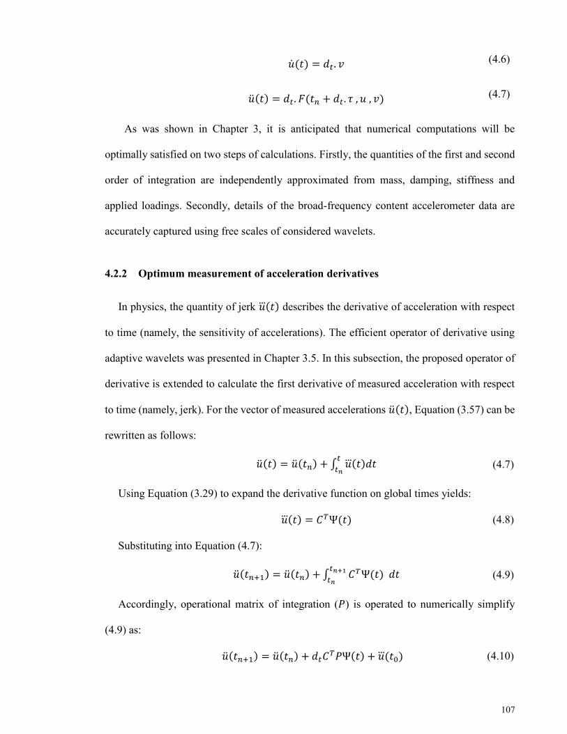
107

�̇�(𝑡) = 𝑑𝑡. 𝑣 (4.6)

�̈�(𝑡) = 𝑑𝑡. 𝐹(𝑡𝑛 + 𝑑𝑡. 𝜏 , 𝑢 , 𝑣) (4.7)

As was shown in Chapter 3, it is anticipated that numerical computations will be

optimally satisfied on two steps of calculations. Firstly, the quantities of the first and second

order of integration are independently approximated from mass, damping, stiffness and

applied loadings. Secondly, details of the broad-frequency content accelerometer data are

accurately captured using free scales of considered wavelets.

4.2.2 Optimum measurement of acceleration derivatives

In physics, the quantity of jerk �⃛�(𝑡) describes the derivative of acceleration with respect

to time (namely, the sensitivity of accelerations). The efficient operator of derivative using

adaptive wavelets was presented in Chapter 3.5. In this subsection, the proposed operator of

derivative is extended to calculate the first derivative of measured acceleration with respect

to time (namely, jerk). For the vector of measured accelerations �̈�(𝑡), Equation (3.57) can be

rewritten as follows:

�̈�(𝑡) = �̈�(𝑡𝑛) + ∫ �⃛�(𝑡)𝑑𝑡𝑡

𝑡𝑛 (4.7)

Using Equation (3.29) to expand the derivative function on global times yields:

�⃛�(𝑡) = 𝐶𝑇Ψ(𝑡) (4.8)

Substituting into Equation (4.7):

�̈�(𝑡𝑛+1) = �̈�(𝑡𝑛) + ∫ 𝐶𝑇Ψ(𝑡) 𝑑𝑡𝑡𝑛+1

𝑡𝑛 (4.9)

Accordingly, operational matrix of integration (𝑃) is operated to numerically simplify

(4.9) as:

�̈�(𝑡𝑛+1) = �̈�(𝑡𝑛) + 𝑑𝑡𝐶𝑇𝑃Ψ(𝑡) + �⃛�(𝑡0) (4.10)

108

Calculating 𝐶𝑇 (corresponding to the global times) and considering initial condition of

�⃛�(𝑡0) and substituting into Equation (4.8), the first-ordered derivative of acceleration with

respect to time (namely, acceleration sensitivity) is numerically approximated. The quantity

of jerk is one of the very sensitive dynamic quantities to the small changes in measured

outputs (that mostly are accelerations). Thus, it will be shown later that our proposed method

for structural damage detection also concerns with the evaluation of this quantity rather than

acceleration itself. However, to enhance the computational efficiency of the proposed

procedure in this research, the very optimum computation of jerk is developed by using

adaptive wavelet functions on longer time intervals. To clarify the aforementioned concept,

a simple example is given in Figure 4.1. Figures 4.1(a) and 4.1(b) show an arbitrary

displacement and relative acceleration time-history, respectively. An impact is imposed to

the system (i.e., due to the loss in stiffness) at the third second of evaluation. The

effectiveness of the proposed idea for optimum analysis of jerk using various scales of

wavelet functions (shown in right-hand column) is compared with the normal incremental

computation of derivatives (illustrated in the left-hand column). For each case (each row of

c to g in the figure), the same sampling rate (or time interval of ∆𝑡) is investigated. However,

for a detailed comparison, the number of colocation points considered for wavelet functions

varies with respect to the different time intervals. To be noted that, LW is considered as the

wavelet basis function to evaluate this example.

It was anticipated that, for the purpose of an accurate evaluation of the quantity of jerk,

the maximum sampling rate of 1000 sampling points should be considered e.g., ∆𝑡=0.001,

shown in Figure 4.1 row (c). Although, using such sampling rates diversely affects the

computational efficiency of the evaluation strategy. Significantly, this figure demonstrates

the effectiveness of the proposed method to optimally compute the sensitivity with the

109

considerable lesser sampling rates of only 2 points e.g., ∆𝑡=0.5 on the compatible collocation

points of wavelet e.g., 2𝑀=4 or 8 shown in Figure 4.1 rows (f) or (g). It is apparent from the

figure that, the proposed method magnificently detect the sudden changes in output signal

through the very optimum computations. However, it will be shown later that the choice of

sampling rate and number of adaptive collocation points should be accurately decided for

integrating the broad frequency contents of the measured (output) signal. It should be pointed

out that, the large-scaled structural systems and correspondingly measured data are the focus

of interest in the most practical cases. In other words, the computational performance of

identification strategy will be considerably enhanced by using an optimum operation for

evaluation of very excessively large data.

4.2.3 Stiffness identification

The optimum measurements of responses were discussed for SDOF mechanical systems,

emphasizing on only the measurement of one DOF. However, the proposed strategies are

applicable for MDOF systems where the measurement of dynamic responses of each DOF

may be considered. Accordingly, assumption of known mass and damping, the time-history

of stiffness in Equation (4.1), is determined by solving Equation (3.40). For this purpose,

quantities of measured acceleration, displacement and velocity are acquired from Equations

(4.2), (4.4) and (4.5). To be noted that, the only one natural frequency of (𝜔 = √(𝑘) (𝑚)⁄ )

is obtained for the proposed SDOF oscillator in Equation (4.1). Consequently, the

distinguishable influence of the proposed wavelet-based procedure of structural

identification is efficiently capturing the broad-frequency contents of external loading 𝐹(𝑡).

Eventually, fast and accurate computations constitute the main advantage of the proposed

method for online health monitoring.

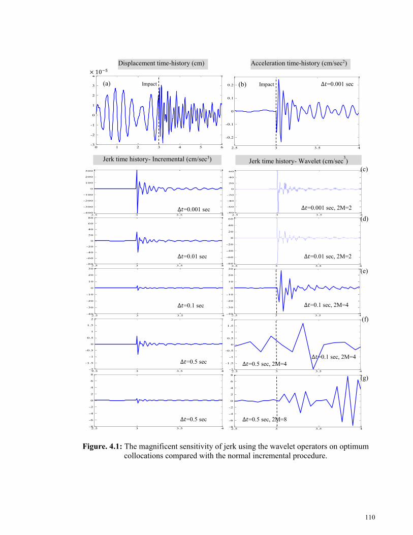
110

Figure. 4.1: The magnificent sensitivity of jerk using the wavelet operators on optimum

collocations compared with the normal incremental procedure.

0 1 2 3 4 5 6-3

-2

-1

0

1

2

3

4x 10

-5

2.5 3 3.5 4

-0.2

-0.1

0

0.1

0.2

2.5 3 3.5 4-8

-6

-4

-2

0

2

4

6

8

2.5 3 3.5 4-400

-300

-200

-100

0

100

200

300

2.5 3 3.5 4-80

-60

-40

-20

0

20

40

60

2.5 3 3.5 4-80

-60

-40

-20

0

20

40

60

2.5 3 3.5 4-40

-30

-20

-10

0

10

20

30

2.5 3 3.5 4-2

-1.5

-1

-0.5

0

0.5

1

1.5

2

2.5 3 3.5 4-2

-1.5

-1

-0.5

0

0.5

1

1.5

2

2.5 3 3.5 4-80

-60

-40

-20

0

20

40

60

80

2.5 3 3.5 4-40

-30

-20

-10

0

10

20

30

2.5 3 3.5 4-8

-6

-4

-2

0

2

4

6

8

Acceleration time-history (cm/sec2) Displacement time-history (cm)

Impact Impact

∆𝑡=0.1 sec, 2M=4

∆𝑡=0.001 sec

Jerk time history- Wavelet (cm/sec3) Jerk time history- Incremental (cm/sec3)

∆𝑡=0.001 sec

∆𝑡=0.5 sec, 2M=4 ∆𝑡=0.5 sec

∆𝑡=0.001 sec, 2M=2

∆𝑡=0.01 sec, 2M=2

∆𝑡=0.1 sec, 2M=4

∆𝑡=0.5 sec

∆𝑡=0.01 sec

∆𝑡=0.1 sec

∆𝑡=0.5 sec, 2M=8

(a) (b)

(c)

(d)

(e)

(f)

(g)

× 10−5

111

4.3 Structural identification of MDOF systems using genetic algorithms

Basically, structural identification of MDOF systems is a more controversial challenge

rather than SDOF ones. In this regard, there are many unknown parameters should be

identified corresponding to the number of structural DOFs (for shear structures) or structural

elements (i.e. identification of structural mass, damping and stiffness). Moreover, it is very

important to keep in mind that in many practical structural identifications, output-only (O-

only) measurements are available and force identification should also be considered.

Accordingly, solving the governing optimization problem on the MDOF system with

measured inputs, is one of the popular options to identify unknown dynamic parameters.

Over the last two decades, solution of optimization problems has been undergone to the

significant improvements. Two well-known strategies of genetic algorithms (GAs) and

neural network (NN) have demonstrated their efficiency in various subjects of science and

engineering. The basic neural network comprised of three layers, an input, hidden and output

layer. The inputs may be fed by proper weighting of the connections and using simple

functions at the neurons to reach at the outputs for linear or non-linear systems. The main

advantage of NN is the possibility of training the network. However, this also constitutes the

main drawback of NN where for identification of large-scaled systems, huge amount of data

are required for the appropriate training. As a consequence, incorrect values will be identified

if incomplete pattern data is measured.

The identification procedure utilized in this research for the solution of inverse problems

lies on genetic algorithms which are inspired by Darwin’s theory of natural selection and

survival of the fittest. For this purpose, in subsequent sections the employment of simple GA

is concerned for structural identification, and then the proposed improvement of GAs strategy

112

will be introduced. The core of developed GAs is structured based on using adaptive wavelet

functions which was discussed in previous chapter and sections.

Fundamentally, there are two possible aspects can be proposed for time-domain structural

identification capable of utilizing wavelet analysis through GAs shown in Figure 4.2.

Figure 4.2: The proposed approaches capable of using adaptive wavelets through GAs,

(a) for initial and rough identification, (b) for accurate and reliable identification.

Measure accelerations and input

forces {�̈�(𝑡) }, {𝑓(𝑡)}

Define global window width, time

interval ∆𝑡 and 2𝑀 adaptive

collocations for each wavelet basis

function

Simulate dynamic equilibrium:

[M] {�̈�(𝑡) } + [C] {�̇�(𝑡) } +

[K] {𝑢(𝑡) } ={𝑓(𝑡) }

to calculate wavelet coefficients and

then computing the simulated {�̈�(𝑡) }.

Conduct GAs to identify unknown

parameters [M], [C] and [K]:

Evaluate simulated and

measured {�̈�(𝑡) }, to proceed the

optimizer.

Extract wavelet coefficients (CW) of

measured quantities: {�̈�(𝑡) }𝑐𝑤

,

{�̇�(𝑡) }𝑐𝑤, {𝑢(𝑡) }

𝑐𝑤, {𝑓(𝑡) }

𝑐𝑤.

Measure accelerations and input

forces {�̈�(𝑡) }, {𝑓(𝑡)}

Define global window width, time

interval ∆𝑡 and 2𝑀 adaptive

collocations for each wavelet basis

function

Decompose measured {�̈�(𝑡) } to

approximate measured velocities

{�̇�(𝑡) } and displacements {𝑢(𝑡) } (Equations 4.2, 4.3 and 4.4).

Construct new dynamic equilibrium:

[M]{�̈�(𝑡) }𝑐𝑤

+ [C]{�̇�(𝑡) }𝑐𝑤

+

[K]{𝑢(𝑡) }𝑐𝑤

= {𝑓(𝑡) }𝑐𝑤

.

Conduct GAs to identify unknown

parameters [M], [C] and [K]:

Evaluate simulated and measured

{�̈�(𝑡) }𝑐𝑤

to proceed the optimizer.

(a) (b)

113

As illustrated in Figure 4.2, the first procedure (a) concerns with adopting GAs on the

wavelet coefficients of responses and input forces which are mostly very small values. As a

consequence, even by normalizing the unknown parameters to small values to overcome the

computational difficulties, most of the time the solution of inverse problem lies on ill-

condition problem and the accuracy of approximate solution degrades. In contrast, the second

procedure (b) concerns with the comparison of simulated responses against measured

responses to process the GAs strategy. From the preliminary investigation carried out on

several applications, it is concluded that results of the first approach are not sufficiently

accurate, and therefore the identification is less reliable. However, the computational process

is faster than the second procedure especially by using longer time windows. For this reason,

the first approach (a) may be preferred as initial predictions while for accurate corrections

and therefore reliable identification the second strategy is strongly recommended.

4.3.1 Simple GAs

The major early work on adaption based on GAs was by John H. Holland (Goldberg and

Holland, 1988). Adaption is regarded as a process of progressive variation of structures,

leading to an improved performance. He recognized the similarities between natural and

artificial systems. Recognizing that operators such as crossing over and mutation that act in

natural systems were also presented in many artificial systems. GAs are search algorithms

that combine a survival of the fittest mentality with a structured and random one and then

exchange information in order to explore the search space. Mathematically, it is achieved by

representing possible solutions as coded strings. Many such strings are created and each

representing a different location on the given search space. These strings are then evaluated

according to some criteria, and the fittest are given a higher probability of selection. Parts of

the selected strings are combined to form new strings and occasionally part of the string is

114

randomly assigned a new value. The method is similar to human search where good solutions

receive more attention while bad solutions are less favored. The overall layout of a simple

GA strategy is depicted in Figure 4.3.

Figure 4.3: Overall layout of a simple GA.

Figure 4.4: Representation and storage of a simple GAs for the identification problems

comprised of n structural elements.

Record the output as the best result (global optima)

Generate initial population

Convert binary strings to

real

No

Yes

Fitness evaluation

Reproduction

Operate crossover

Operate mutation

Pi

𝒌𝟏 𝒌𝟐 … 𝒌𝒏 𝒎𝟏 𝒎𝟐 … 𝒎𝒏 α β

Individual 1:

Generation no. 1, contains i populations

…..




Individual j-1:

Individual j:

Individual 2:

P2

P1

….

Population 1 (P1),

contains j individuals

String 1 (all strings are

binary encoded) String 2n+2

Satisfied?

115

As shown in Figure 4.3, a simple GA is based on binary encoding. As a consequence,

operations of mutation and crossover will be executed only uniformly, however, it will be

discussed later that to enhance the performance of GAs strategies, implementation of non-

uniform operators of mutation and crossover is essential. Some of the basic features of a

simple GA is illustrated in Figure 4.4 for structural identification through an inverse problem.

Figure 4.4 shows the capability of GA with different performances to find the global optima.

In performing a GA strategy, the reliability and robustness of the solution is very important.

The population size (number of individuals) involving j number of fixed 2n+2 strings

(referring to n structural elements) and number of populations in each generation are taken

after an engineering judgment about the either prescribed convergence of results or

computational efficiencies.

It is also possible to influence the search by selecting appropriate crossover and mutation

rates, however in general, there is a trade-off between exploration (broad search) and

exploitation (local search). For instance, small crossover and mutation rates help explore the

domains around the current solutions, and thus are less likely to destroy good solutions.

Although, it will make it more difficult to explore new possible solutions. On the other hand,

large crossover and mutation rates help to cover wider domains, however at the expense that

the desirable solutions are less likely to develop further and thus they find it harder to

converge.

4.3.1.1 Fitness evaluation and selection

Two underlying features of any GAs strategy are the fitness evaluation of possible

solutions and accordingly selection of good results. For the purpose of fitness evaluation, the

response of structure i.e., acceleration is numerically simulated using the proposed wavelet-

based approach for the predicted properties of structure (generated in different strings). On

116

the other hand, the actual response of structure have been measured for each existing DOF

of structure. Consequently, one may evaluate the fitness function as follows (Perry, Koh, and

Choo, 2006):

𝐹𝑖𝑡𝑛𝑒𝑠𝑠 =1

0.001 +𝑀𝑆 (4.11)

where, 𝑀𝑆 is the difference between measured and simulated responses. Thus, this value

is obtained as follows:

𝑀𝑆 =∑(𝑀𝑒𝑎𝑠𝑢𝑟𝑒𝑑 − 𝑠𝑖𝑚𝑢𝑙𝑎𝑡𝑒𝑑)2

𝑀𝑒𝑎𝑠𝑢𝑟𝑒𝑑 𝐷𝑂𝐹𝑠 (4.12)

As it is shown in Equation (4.12), the fitness is evaluated from the total sum of square

error between the simulated and measured response of the structure at each time step. Finally,

this value is divided by the total measured DOFs. This function bounds the maximum fitness

at 1000 showing that, when errors approach zero (𝑀𝑆=0), results have converged. In addition,

final selection will be carried out using roulette wheel procedure based on the maximum

probability of selection for fitted individuals. The step-by-step algorithm of simple GA using

adaptive wavelet functions is tabulated in Table (4.1).

It should be emphasized that according to the simple GA, the rate of crossover and

mutation can be reduced from the initial populations to the later ones in a single generation.

Therefore, the exploration (global search for promising solutions) and exploitation phases

(local search around optima) of GA strategy will be proceeded much more properly.

117

Table 4.1: Step-by-step algorithm of simple GA using adaptive wavelet functions.

C. Initial calculations:

(11) Define upper and lower limits for unknown variables (mass: Mi, damping ratio:

Di, stiffness: Ki). i refers to the i th DOF.

(12) Define the required precision for each variable.

(13) Define the crossover and mutation rate.

(14) Define the geometry of structure.

(15) Define the number of required populations in a single generation as well as the

population’s size.

(16) Specify the location of each variable on corresponding strings.

(17) Randomly generate the initial population (0 or 1 due to binary encoding).

(18) Specify wavelet basis function, number of collocation points, the considered

order of wavelet based on the sampling rate of the measured responses.

(19) Select an appropriate time step 𝒅𝒕 (concerning an efficient solution).

(20) Form coefficients wavelet matrix corresponding to collocation points for free-scaled

orders of wavelet function 𝝓(𝒕). (21) Form operation matrix of integration corresponding to collocation points for each

particular wavelet function 𝑷.

(22) Calculate square operational matrix 𝑷𝟐.

(23) Approximate unity, with related coefficient of wavelets.

(24) Form identity matrix of 𝑰 on collocation points.

D. For each iteration:

(5) Convert binary strings to real value for each individual.

(6) For each individual form the properties matrices (predicted mass: M, damping ratio:

D, stiffness: K) using the known geometry and structures behavior (i.e., MDOF shear

building, 2D pin-jointed truss, 3D truss and so on).

(7) Use the proposed method of time integration (wavelet-based method) to solve

simulated responses of dynamic equilibrium: 𝐌 �̈�(𝑡) + 𝐂 �̇�(𝑡) + 𝐊 𝑢(𝑡) = 𝐹(𝑡) (8) For each DOF or member, corresponding to each individual, calculate displacement,

velocity and acceleration vectors at each time interval, simultaneously by:

𝑢(𝑡) = 𝐶𝑇𝑃2Ψ(𝑡) + 𝑢𝑛0

�̇�(𝑡) = 𝐶𝑇𝑃Ψ(𝑡) + 𝑣𝑛0

�̈�(𝑡) = 𝐶𝑇Ψ(𝑡)

(9) Evaluate the fitness function using Equation (4.11).

(10) Investigate the rate of convergence of responses. If results are converged then

exit iteration and record the identified values as the actual values; if not, continue to

next step.

(11) Perform the roulette wheel selection method.

(12) Rearrange and sort the whole population’s individuals from the best fit to the

worst.

(13) Pair individuals.

(14) Operate crossover and mutation to paired individuals.

(15) Go to step B. (1).

118

4.3.2 Modified multi-species GAs

Over the past two decades, there are diverse forms of GAs have been widely improved. A

fundamental coding was using binary representation for simple GAs and set of operators i.e.,

crossover, mutation and reproduction. More recently, much efforts have also been made to

alter the architecture of GA to be practical for solving complex problems. One of the popular

modified GA (MGA) utilizes migration and artificial selection for real encoding variables.

The underlying components that distinguish this strategy are not only inclusion of multi-

species (sub-populations) but also a rank based selection and a new tagging procedure to

ensure diversity in the best solutions (Michalewicz, 2013). In contrast to the simple GAs, the

proposed multi-species strategy here is real encoded and as such adopts non-uniform

operators. Floating point representation allows the focus of the search to vary, not just across

species, but also over time. Therefore, the main advantage of performing multi-species is that

various GA-based operators can be implemented to complement one another.

4.3.3 Wavelet-based MGAs

The proposed wavelet-based MGAs (WMGA) strategy in this research is benefitted by a

computationally efficient scheme for fitness evaluation using adaptive wavelet functions.

This enables using more sub-populations within a population and increasing the convergence

of results and therefore improving computational competency and robustness of structural

health monitoring strategies. The proposed procedure is developed in order to provide a

reliable identification algorithm for large-scaled structures that simultaneously explores the

search domain and focuses on promising individuals. The construction of the proposed

WMGA strategy utilized in this research is depicted in Figure 4.5.

119

Figure 4.5: The construction of the proposed multi-species population capable of using

WMGA.

Accordingly, the adopted WMGA strategy to identify unknown dynamic parameters is

discussed in detail as following subsections.

4.3.3.1 Modification of multi-species populations

As shown in Figure 4.5, each population involves 6 species with different GA-based

operators. In this section the corresponding features of each species 1 to 6 are elaborated.

𝑘1 𝑘2 … 𝑘𝑛 𝑚1𝑚2 …𝑚𝑛 α β

Species 1:

It stores the best fitted individuals and to avoid skipping

the optimum solution.

Crossover Simple

Multi-point

Species 2: For random

search/reproduction

Mutation Random

Crossover Simple

Multi-point

Species 3: For cyclic

search/reproduction

Mutation Cyclic non-linear

Crossover ABX

Species 4: For average bound

search/reproduction

Mutation WM

Crossover SBX

Species 5: For simulated binary

search/reproduction

Mutation PM

Crossover Simple

Multi-point

Species 6: For local search and

focusing on local optima

Mutation Non-linear local

T Ra Rj

Per

iod

ically

ring

op

erato

r of m

igra

tion

120

The first species:

Essentially, there is no GA-based operators are employed on this species so as this sub-

population is solely designed to store the best results. The tagging procedure (designated by

string T in Figure 4.5) prevents saturating this species by selecting a same individual many

times. For this purpose, all individuals are initially assigned 0 as tag number and if an

individual being selected for species 1 the tag is changed to 1. This tag follows individual

wherever it goes until this individual being altered by any GA-based operator, in this case

the tag will be changed back to 0, denoting a new individual and making it available to be

selected as the best solutions for species 1.

The second species

The crossover operators utilized for species 2, 3 and 6 lies on the simple and multi-points

operators of crossover. Assumption of 𝑃𝑐𝑠 and 𝑃𝑐𝑚 for the probability of simple and multi-

point crossover operations, the total crossover rate 𝑃𝑐𝑡 which shows the effective probability

rate of an individual being involved in at least one crossover is as follows (Perry et al., 2006):

𝑃𝑐𝑡 = 1 − (1 − 𝑃𝑐𝑠)(1 − 𝑃𝑐𝑚) (4.13)

Furthermore, species 2 is designed for a wide and random search for possible optima

within the search limits prescribed for unknowns. To randomly generate new possibilities, a

random real number is generated as 𝑟 ∈ [0 1] and the random mutation is developed by:

𝑥𝑖 = 𝐿𝐿𝑖 + 𝑟 × (𝑈𝐿𝑖 − 𝐿𝐿𝑖) (4.14)

In Equation (4.14), 𝑥𝑖, 𝐿𝐿𝑖 and 𝑈𝐿𝑖 indicate the ith altered unknown (parameter), the ith

lower and upper limits of the search domain, respectively.

121

The third species

Mathematically, it is demonstrated that the accuracy and convergence rate of optimization

problems are influenced by operating the so-called non-uniform mutation. This is because of

the reduction of the average magnitude of mutations during the procedure of optimization

(Michalewicz, 2013). The mutation operator designated for species 3 lies on the cyclic non-

uniform mutation. The underlying principal is to slightly reduce the number of mutations as

the optimizer proceeds. Logically, this operator will increase again after the regeneration, to

allow a broad search for possible solutions. Assumption of a random real number 𝑟1 ∈ [0 1]

and random integer 𝑟2 ∈ [0 1], the operator of cyclic non-uniform mutation is obtained as

follows (Perry et al., 2006):

𝑥𝑖 = 𝑥𝑖 + (𝑈𝐿𝑖 − 𝑥𝑖) × (1 − 𝑟1(1−

0.9𝑀𝑂𝐷(𝑔,𝑅)𝑅

)) 𝑖𝑓 𝑟2 = 0

𝑥𝑖 = 𝑥𝑖 + (𝐿𝐿𝑖 − 𝑥𝑖) × (1 − 𝑟1(1−

0.9𝑀𝑂𝐷(𝑔,𝑅)𝑅

)) 𝑖𝑓 𝑟2 = 1

(4.15)

In Equation (4.15), 𝑔 and 𝑅 denote the generation number and the number of generations

between regenerations, respectively. In addition, 𝑀𝑂𝐷 represents the operation of reminder.

The forth species

The Average and Bound crossover (ABX) is proposed as the crossover operator of this

species. This operator was adopted by Ling and Leung (2007). However, they did not concern

with the improvement of fitness evaluation (FE), as this operator requires inner FE and from

the computational cost point of view is inherently a costly operator, especially for large-

scaled structures with the numerous unknowns to be identified. Based on this method, four

122

offspring (𝑜1 − 𝑜4) are obtained from two parents (𝑝1and 𝑝2) in new generation, including

two of the average (𝑜1and 𝑜2) and two of the bound (𝑜3and 𝑜4) crossover as follows:

𝑜1 =𝑥𝑖𝑝1 + 𝑥𝑖

𝑝2

2

𝑜2 =(𝑈𝐿𝑖 + 𝐿𝐿𝑖)(1 − 𝜔𝑎) + (𝑥𝑖

𝑝1 + 𝑥𝑖𝑝2)𝜔𝑎

2

𝑜3 = 𝑈𝐿𝑖(1 − 𝜔𝑏) + max(𝑥𝑖𝑝1 , 𝑥𝑖

𝑝2)𝜔𝑏

𝑜4 = 𝐿𝐿𝑖(1 − 𝜔𝑏) + min(𝑥𝑖𝑝1 , 𝑥𝑖

𝑝2)𝜔𝑏

(4.16)

Ling and Leung (2007) suggested that however the weight factor 𝜔𝑎 could be selected

1, the range of [0.5 1] is reasonable. In addition, they adopted 𝜔𝑏 ∈ [0 1] for several

numerical investigations. The FE of 𝑜1 − 𝑜4 will be carried out and the fitted offspring will

be selected. Subsequently, the mutation operator of species four is a wavelet-based mutation

(WM) proposed by Ling et al. (2007). Assumption of 𝑈𝐿𝑖𝑚𝑎𝑥 and 𝐿𝐿𝑖

𝑚𝑖𝑛 as the maximum

and the minimum value for upper and lower limits of unknowns in an individual, the WM

mutation is obtained as follows:

𝑥𝑖 = {𝑥𝑖 + 𝛿(𝑈𝐿𝑖

𝑚𝑎𝑥 − 𝑥𝑖) 𝑖𝑓 𝛿 > 0

𝑥𝑖 + 𝛿(𝑥𝑖 − 𝐿𝐿𝑖𝑚𝑖𝑛) 𝑖𝑓 𝛿 ≤ 0

𝛿 =1

√𝑎𝑒−(𝜑/𝑎)2

2 cos (5 (𝜑

𝑎)) ; 𝜑 ∈ [−2.5,2.5]

𝑎 = 𝑒− log(𝛾)(1−𝑔 𝐺⁄ )𝜁+log(𝛾)

(4.17)

In Equation (4.17), 𝑔, 𝐺 and 휁 represent the generation counter, the total number of

generations and the shape parameter of the monotonic increase (휁 ∈ [0.2,5]). 𝛾 is the upper

limit of parameter a and could be assigned 10000. To be noted that, this operator behaves as

a local search mutation, however it just designed to locally search around the promising

random results in only species four and not for fine-tuning search on the best results of the

123

whole population. To overcome this issue, the presented WMGA strategy in this research

complemented with the sixth species, as well.

The fifth species

The crossover operator designed for this species is the Simulated Binary crossover (SBX)

adopted by Deb and Agrawal (1994). Assumption of 휂𝑐=2 (Deb and Gulati, 2001) as a

parameter to control the spread, SBX is derived as follows:

𝑜1 = 0.5[(𝑥𝑖𝑝1 + 𝑥𝑖

𝑝2) − 𝛽|𝑥𝑖𝑝2 − 𝑥𝑖

𝑝1|]

𝑜2 = 0.5[(𝑥𝑖𝑝1 + 𝑥𝑖

𝑝2) + 𝛽|𝑥𝑖𝑝2 − 𝑥𝑖

𝑝1|]

𝛽 =

{

(2𝑟1)

1𝜂𝑐+1 𝑖𝑓 𝑟1 ≤ 0.51

2(1 − 𝑟1)1

𝜂𝑐+1

𝑜𝑡ℎ𝑒𝑟𝑤𝑖𝑠𝑒

(4.18)

In Equation (4.18), 𝑟1 is a real random number as introduced earlier. Accordingly, the

Parametric-based mutation (PM) operator proposed by Deb and Gulati (2001) is considered

for this species. Basically, it performs a polynomial probability distribution to generate a

mutated individual in the neighborhood of the original one. Let 𝑟1 a real random ∈ [0 1] for

problems concerning the upper and lower bounds it is obtained as follows:

𝛿̅ = {[2𝑟1 + (1 − 2𝑟1)(1 − 𝛿)

𝜂𝑚+1]1

𝜂𝑚+1 − 1 𝑖𝑓 𝑟1 ≤ 0.5

1 − [2(1 − 𝑟1) + 2(𝑟1 − 0.5)(1 − 𝛿)𝜂𝑚+1]

1

𝜂𝑚+1 𝑜𝑡ℎ𝑒𝑟𝑤𝑖𝑠𝑒

𝛿 = min[(𝑥𝑖 − 𝐿𝐿𝑖), (𝑈𝐿𝑖 − 𝑥𝑖)] /(𝑈𝐿𝑖 − 𝐿𝐿𝑖)

(4.19)

In Equation (4.19), 휂𝑚 is the distribution index for mutation and takes any non-negative

value. This value regulates the achieved perturbation and may be selected around 100 to gain

the mutation effect of 1%. To be emphasized that the total number of mutated individuals

𝑁𝑚for each species is defined and so the species size remains constant after reproductions.

124

The sixth species

Species 6 is designed to focus on the local optima (i.e., the local search around the best

results). For this purpose, small mutations are employed to refine the best solutions by

operating a non-uniform mutation, whereby the mutation rate is slightly reduced as the

optimization proceeds. The following mutation operator is considered to accomplish this goal

(Perry et al., 2006):

𝑥𝑖 = 𝑥𝑖 + 0.5 × (𝑈𝐿𝑖 − 𝑥𝑖) × (1 − 𝑟1(1−

𝑔𝐺)) 𝑖𝑓 𝑟2 = 0

𝑥𝑖 = 𝑥𝑖 + 0.5 × (𝐿𝐿𝑖 − 𝑥𝑖) × (1 − 𝑟1(1−

𝑔𝐺)) 𝑖𝑓 𝑟2 = 1

(4.20)

In Equation (4.20), 𝐺 denotes the total number of generations to be run. Finally, a periodic

operator of ring migration is designed to exchange the best results between species 2 to 6 as

shown in Figure 4.5. This operator is regulated based on two parameters 𝑧1 and 𝑧2. The first

parameter controls the number of generations between two migrations whereas the second

one is the fraction of species size involved in the migration. In this study, 𝑧1=5 and 𝑧2=0.1-

0.2 are utilized as the periodicity of the operator and the portion of sub-population to be

involved in migration, respectively.

4.3.3.2 Modified search space reduction technique

Basically, the convergence rate and accuracy of the GA-based identification strategies are

highly dependent to the width of the search space. As a consequence, by adaptively reducing

the search limits, a more satisfactory identification is possible with the best computational

efficiency (Perry et al., 2006). The SSRM strategy implemented in this study is illustrated in

Figure 4.6.

125

Figure 4.6: The proposed SSRM strategy capable of using adaptive wavelets for

optimum identification through WMGA.

As it is shown in Figure 4.6, the proposed SSRM involves a very fast prediction and

therefore reduction of initial search limits by using simple and 2D Haar wavelets on optimum

collocations (2𝑀P). This phase may be interpreted as exploration phase and there is the most

relevant variations around local optima. It should be emphasized that, initial search limits, in

fact, lies on a wide limits for unknown parameters. At the second stage of the strategy, the

search limits have been refined by using 3D LW for fitness evaluation of individuals as the

same sampling rate as was considered for the first step. To ensure capturing all features of

I/O signal more collocation points (2𝑀R) are preferred at this stage. Accordingly, this stage

is adopted for exploitation phase where the small variations around the global optima is

existed. Finally, employing the accurate SCW for fitness evaluation guarantees the promising

solutions being selected. In this regards, all details of I/O signals are collectively captured on

adaptive collocation points (2𝑀C), and therefore the last corrections of unknowns are

optimally ascertained until the prescribed convergence rate is achieved (namely, the final

(Gen×Run)

Sta

rtin

g s

tep

, in

itia

l w

ide

lim

its

assu

med

for

var

iab

les

Haar Wavelet

Initial and fast

evaluations to

optimally shorten

the limit bands

(Prediction/

Exploration

phase)

∆𝑡, 2MP ∆𝑡, 2MP<2MR

LW

First modification

of populations

and reducing the

limit bands

(Refinement/ Exploitation

phase)

∆𝑡, 2MR<2MC

SCW

Final corrections

to ensure

capturing broad

frequency

contents (Correction/

Exploitation

phase) Op

tim

um

id

enti

fica

tio

n o

f u

nkn

ow

n

var

iab

les

SSRM SSRM

126

exploitation phase). The motivation behind the proposed development arises from the fact

that the overall computational efficiency of the identification strategy for large number of

unknowns is rigorously dependent on optimally reducing the search limits with the emphasis

on accuracy of results.

4.3.3.3 Fitness evaluation and artificial selection

Eventually, the fitness of each individual in all species proposed in this study are evaluated

by adding the inverse of total sum of square errors between the measured and simulated time-

history of accelerations for off-line applications and the quantities of jerk for online

identification problems as follows:

𝐹𝑖𝑡𝑛𝑒𝑠𝑠 =

1

휀 +∑(𝐴𝑐𝑐𝑚𝑒𝑎𝑠. − 𝐴𝑐𝑐𝑠𝑖𝑚𝑢.)2

𝐷𝑂𝐹𝑚𝑒𝑎𝑠.

+1

휀 +∑(𝑗𝑒𝑟𝑘𝑚𝑒𝑎𝑠. − 𝑗𝑒𝑟𝑘𝑠𝑖𝑚𝑢.)2

𝐷𝑂𝐹𝑚𝑒𝑎𝑠.

(4.21)

In Equation (4.21), DOF, meas. and simu. represent the total measured DOFs, measured

and simulated data, respectively. 휀 may takes a small value of 0.001 to prevent computational

difficulties. In this research, the first term in Equation (4.21) is proposed for the fitness

evaluation due to the analysis of accelerations (designated by Fita) and the second term is the

fitness due to the jerk analysis (designated by Fitj). Later, the selection procedure is carried

out by allocating the probability of selection to each individual due to its final fitness. To

magnify the differences between different fitness values, a ranking procedure is employed to

obtain the probabilities within each species. In other words, the fitted individual is ranked the

total number of population size and the rest are descended due to the value of the fitness

function for both Fita and Fitj. The notable point on the proposed fitness evaluation (FE) lies

on the sufficiently optimum evaluation of Fitj by wavelet functions for the small sampling

rates (in referring to Figure 4.1). This significantly improves the fitness values and rapidly

yields the convergence rate. It will be shown later that in practical and large-scaled

127

applications, whereby there is a loss in stiffness concurrent to the system identification

(referring to the online damage imposed), by employing the second term of FE in Equation

(4.21), not only the place of imposed impact on time axis but also the magnitude of the

reduction in stiffness are confidently detected. In this research, LW(2M4) is performed with

very small sampling rate of 20 S/s (∆𝑡 = 0.05 sec compared to the acquired ∆𝑡 = 0.001 sec)

for the effective jerk-based FE of all species. As it was mentioned before, the fast and precise

computation of LW increases the computational competency of the proposed FE and leads

the reasonably reliable online identification.

4.3.3.4 Practical algorithm of WMGA strategy

The optimum structural identification strategy is achieved by adopting the non-

conventional wavelet-based GA operators (namely, WMGA). The procedure involves

reintroduction, regeneration and artificial selection of ranked individuals. To guarantee that

species 6 (designed for the local search around the best results) operates on a set of desirable

solutions the reintroduction is necessary. This comprises copying individuals from species 1

(the best solutions) into species 6 at a prescribed period. The number of times that

reintroduction should be done must consider that the best solutions require to be developed,

and that species 6 requires some time to improve possible solutions, however, it is found that

a large number of reintroductions commonly gains the better results. In addition, a common

issue of GA-based strategy is that the optimization may be converged to the local optima. To

overcome this issue a regeneration operator is designed for species 2 to 5 and the process will

be effectively started to find global optima and new possibilities while species 6 focuses on

refining the previously generated individuals. The schematic flowchart of the proposed

WMGA is depicted in Figure 4.7.

128

Figure 4.7: The proposed WMGA strategy by using adaptive wavelet functions.

To be noted that the fitness evaluation corresponding to online identification problems

(referring to the presence of damage concurrent with measurement) contains the jerk

evaluation (Fitj) by using LW (2M4) at 20 S/s sampling rates. With reference to Figure 4.6,

three runs are carried out for 3 times of search space reductions corresponding to Haar, LW

Y

N

Y N Return the identified results

from the first row (species 1) as

the best results

N

Ru

n=

Ru

n+

1

Max Gen?

Start WMGA

Random generation

of initial Pop Run=1

If Run==1 then; select Haar wavelet, proper 2M and

∆𝑡 If Run==2 then; select LW, proper 2M and ∆𝑡 If Run==3 then; select SCW, proper 2M and ∆𝑡

SSRM Y Time for

SSRM? Random generation

of species 2-5 Initialize tagging (T)

and ranking (Ra , Rj) Gen

=1

Time for Regen?

Y

FE for ranked fitness values:

Fitall= Ra Fita + Rj Fitj

Copy

individuals

from species 1

to 6

N

Time for Reintro?

Regeneration of species

2-5 and update tagging

and ranking

Species 2: use the selected basis

function

Species 3: use the selected

basis function


function for local search


function

Species 4: use LW (2M4) at

∆𝑡=0.05 sec for internal

evaluation of ABX for all Runs Fit

j: use LW (2M4) at ∆𝑡=0.05

sec for all Individuals.

Fita: use selected wavelet basis

and proper 2M collocations to

ensure broad frequency contents

are captured

Y

N Gen=Gen+1

Max Run? End WMGA

129

and SCW. To be emphasized that, LW(2M4) is optimally adopted for all runs for internal

fitness evaluation (FE) of species 4. Subsequently, the schematic flowchart for structural

simulation and relatively fitness evaluation is depicted in Figure 4.8.

Figure 4.8: The practical flowchart to optimally simulate dynamic response using

wavelet functions prior to fitness evaluation (FE) of genetic individuals (Ind).

As it is shown in the figure, the starting point for identification of large-scaled structural

systems, undoubtedly is to optimizing the sequence of node numbering. The minimum upper

(or lower) bandwidth of characteristics’ matrices, and thus, the effective computations are

the resultant of optimum sequence of node numbering (especially stiffness matrix, while

mostly a lumped mass considered). To accomplish the most cost-effective identification

Start

Ind=Ind+1 Ind=1

To increase the computational efficiency,

optimum node numbering is essential to achieve

the best sequence of sensor placement

Form global [K], [M] and [C] matrices using

genetic strings data (ki, mi, αi and βi; i=1,2,…,

total number of elements)

Static/Dynamic condensation of global

matrices to obtain reduced [K]r , [M]r and

[C]r on measured and loading DOFs

Compute 𝑢(𝑡) and �̈�(𝑡) using wavelet

functions on adaptive collocation points

N Ind is reached?

Y Send

quantities

�⃛�(𝑡) and �̈�(𝑡) to FE

En

d

130

strategy, whereby the FE is being carried out numerous times, this step is strongly

recommended. We have utilized a GAs procedure based on decimal two-dimensional array

coding for both optimal node numbering and sensor placement strategies (the brief discussion

is provided in Appendices B and C). The next key point should be considered for any robust

identification strategy is that in real cases the measurements of all DOFs are not always

available. For this reason, the identification will be carried out on only measured DOFs and

therefore the effect of unmeasured DOFs should be considered in relative characteristics’

matrices (i.e., mass, damping or stiffness). Two popular methods are referred to static and

dynamic condensation methods in order to condensate the characteristics’ matrices from the

entire DOFs existing in structure to the only measured DOFs (the brief discussion is provided

in Appendices A).

4.4 Modification of WMGA strategy for output-only identification

In reality, measuring input forces in situations outside laboratory is not always feasible.

In this section, the WMGA strategy proposed in previous sections for structural identification

is adopted to cases where the input force(s) is not measured and it is so-called output-only

(O-only) structural identification. Basically, there are many attempts have conducted for

output-only identification using frequency domain methods. The strength and weakness of

these methods were discussed in the second chapter. The most significant researches by Ling

and Haldar (2004) used classical techniques to carry out the identification using an iterative

approach. In addition, aforementioned iterative procedure, while reasonably efficient for a

least squares identification, requires considerable computation time involved for a GA due

to the larger time required for each iteration.

131

In this section, a strategy involving simultaneous evolution of structural parameters and

input force is introduced. The strategy utilizes WMGA to identify and update input force(s)

as the search for structural unknown parameters proceeds. For the strategy proposed here, the

mass of structure is assumed as known parameter since for many real applications this is a

reasonable assumption as the mass may be predicted with sufficient precision. Furthermore,

to modify the WMGA identification for output-only measurements, it is assumed that the

structure is initially at rest and that the location of input force(s) is known. In addition, the

damping is also assumed to be of Rayleigh damping, where the damping parameters are

unknown. The major objective will be to identify time-history of input force(s) and stiffness

parameters. It is to be pointed out that, because of the banded nature of property matrices

(i.e., stiffness and mass), it is also assumed that the acceleration measurements are available

at least at the DOF with unknown force and adjacent (coupled) DOFs.

Fundamentally, the time-history of input force(s) is treated as an unknown component of

dynamic equilibrium in each iteration of WMGA rather than an unknown variable to be

identified by WMGA strategy. In the modified procedure the computation of force is

combined with the wavelet-based algorithm proposed in Chapter 3 for structural simulation.

In this regards, input force is estimated while the strategy simultaneously is carrying out the

simulation of response for evaluation with measured acceleration to calculate the fitness of

the given solution. The proposed WMGA identification strategy lies on a predictor-corrector

algorithm. An initial prediction of the displacements and velocities at measured DOFs at time

step 𝑖+1 is first obtained from the measured accelerations at time step 𝑖+1. Accordingly, the

corrected response at time step 𝑖 is defined as predictor equations of:

�̈�𝑖+1(𝑡) = 𝐴𝑐𝑐𝑖+1𝑚𝑒𝑎𝑠.

= 𝐶𝑇Ψ(𝑡)

�̇�𝑖+1(𝑡) = 𝑑𝑡𝐶𝑇𝑃𝜓(𝑡) + 𝑣𝑖 (4.22)

𝑢𝑖+1(𝑡) = 𝑑𝑡2𝐶𝑇𝑃2𝜓(𝑡) + 𝑢𝑖

132

In Equation (4.22), 𝑑𝑡 is the time step 𝑡𝑖 to 𝑡𝑖+1. 𝑢𝑖 and 𝑣𝑖 represent initial displacement

and velocity calculated from previous time step and taking into account that structure has

been initially at rest (𝑢0 = 𝑣0 = 0). The unknown force 𝐹𝑈𝑛 is therefore obtained from the

known forces 𝐹𝐾𝑛 (may be recorded by available force sensors attached to other DOFs) at

time step 𝑖+1, measured accelerations, predicted displacements and velocities as follows:

𝐹𝑈𝑛𝑖+1 = [𝑀]�̈�𝑖+1(𝑡) + [𝐶]�̇�𝑖+1(𝑡) + [𝐾]𝑢𝑖+1(𝑡) − 𝐹𝐾𝑛

𝑖+1 (4.23)

The indirect wavelet-based method proposed in Chapter 3 is then performed to re-compute

the responses at time step 𝑖+1, and thus it is resulting in corrected or revised estimates of

accelerations, velocities and displacements. The fitness evaluation of WMGA is conducted

on corrected accelerations compared with those of measured ones. The corrected response

will then be implemented on the next time step and the procedure is repeated for the whole

time-history resulting identification of input force(s). It should be emphasized that, the

corrected responses are being utilized at time step 𝑖 in Equation (4.22) rather than the

measured or predicted responses. Consequently, there is no effect of accumulation of errors

due to integration procedure as the corrected (simulated) response is used and the force is not

computed from the response obtained by integration of measured accelerations. It should be

kept in mind that, dynamic equilibrium governing to the structure is maintained at the end of

each time interval as the corrected response have been employed.

4.5 WMGA strategy for structural damage detection

The WMGA developed in previous sections is applied to improve an optimum damage

detection strategy. To be more practical, the proposed scenario of damage detection in this

research utilizes the previous measurements of undamaged structure. However, the

alternative for this is to identify unknown parameters and compare with those of theoretical

133

values. Hence, the proposed strategy illustrated in Figure 4.9 deals with the scenario where

the measurements of the system both before and after damage has taken place are available.

Figure 4.9: The proposed algorithm for damage detection strategy using WMGA.

As shown in Figure 4.9, the proposed strategy for damage detection is performed through

two main steps. The first involving the calibration of unknown parameters of stiffness by

providing the possibility of using identified parameters for the undamaged structure as a

starting point for identification of damaged structure. This constitutes the distinguishable

merit of the proposed strategy, in which that only changes require to be identified and

providing the optimizer a desirable initial points, resulting in satisfactorily precise outcomes.

For this purpose, the half of individuals in species 4 and 6 (were designed for local searches)

Fix search limits for

the mass of damaged

system

Start WMGA

Damage

Detection

Known mass problem and to

identify parameters of damaged

system (SSRM)

N Y

N

Y

Calculate percentile damage index for each structural element

as: (%) 𝐷𝑖 =𝑘𝑖𝑈𝑛𝑑𝑎𝑚𝑎𝑔𝑒𝑑

−𝑘𝑖𝐷𝑎𝑚𝑎𝑔𝑒𝑑

𝑘𝑖𝑈𝑛𝑑𝑎𝑚𝑎𝑔𝑒𝑑 × 100

Identify unknown parameters

of undamaged structures using

WMGA through SSRM for

known or unknown mass

Using

identified

parameters as

an initial step

for damaged

system? Insert identified values as only the

first individual of species 1 and as

every second individual of species

4 and 6 (half).

Fix identified mass as the

mass of damaged system

(known mass)?

Unknown mass problem and to

identify parameters of damaged

system (SSRM)

End WMGA

Damage

Detection

134

and only the first individual of species 1 are initially set as the identified parameters. This

ensure a good performance of the crossover operation at early stages. The second involves

the possibility of fixing the mass to simplify the problem as in fact the mass is not altered

from damaged to undamaged stage. Eventually, the damage index is computed for the

reduction in stiffness of the element as a percentage of the original undamaged stiffness.

4.6 Numerical verification study

The capability and effectiveness of the proposed strategies for structural identification and

damage detection are numerically evaluated in this section. For this purpose, three numerical

applications are considered, involving a MDOF shear system composed of three connected

MDOF structures for structural identification of known and unknown mass problems as well

as force identification. Additionally, two truss structures are considered for identification and

damage detection, including a 2D Parker truss structure subjected to El-Centro base

excitation and a 3D and large-scaled hexagonal space structure under different concentrated

loading scenarios. For both structures only transitional DOFs are existed so that they are

modeled as pin-jointed truss structures. Initially, the configuration of each structure is

modeled in Formex Algebra (FORMIAN) and later the nodal coordinates have been

transferred to MATLAB. Prior to starting any conventional identification or damage

detection strategy, the sequence of node numbering should be optimized in order to construct

the most optimum mass and stiffness matrices (Appendix C).

For all cases considered, the mass of structures is lumped at each transitional DOF.

Furthermore, damping is provided as Rayleigh damping by setting damping ratio of λ% for

the first two modes and using the desirable values for 𝛼 and 𝛽. For this purpose, λ=2 and λ=5

are selected for identification of example 1 and examples 2 and 3, respectively. In addition,

135

the time-history of nodal accelerations is numerically simulated by the well-known average

acceleration method of Newmark- 𝛽 family, using the sampling rate of 200 S/s for the first

example (it will be evaluated as the measured accelerations) and sampling rate of 1000 S/s

corresponding to the truss structures.

Moreover, for truss systems where damage detection is conducted, two kinds of damage

scenarios are considered as damage induced to the structural elements. The first involving

the offline reduction of the stiffness of structural elements that denotes the measurement of

damaged structure (designated by Off). The second being online reduction of stiffness that

represents the damage has taken place on structural elements during the measurement of

damaged structure (designated by On).

Fundamentally, the very important step prior to any identification strategy is selecting

WMGA parameters to be utilized through the strategy. For this purpose, some preliminary

studies were carried out for each numerical applications in order to determine the most

reasonable WMGA parameter values. The underlying purpose of these studies was to identify

balanced WMGA parameters that will give consistently desirable results rather than trying

to find optimum WMGA parameters. It will be shown later that, for each numerical example,

different combinations of WMGA parameters will have different effects due to the variations

across structural systems and external loadings.

Eventually, the computational efficiencies and the robustness of the proposed WMGA

strategy have been compared with some of the available methods. For the purpose of a

comprehensive evaluation, the CPU computational time (as indication of the cost of analysis)

is comparatively considered for different strategies, which was recorded with a same

hardware environment (I-5 CPU @3.2GHz, Operation 64 bit).

136

4.6.1 A MDOF shear building

The computational efficiency and robustness of the proposed WMGA strategy are

evaluated through the first application regarding to the structural identification of I/O data,

known and unknown mass problems, initially. Later, the strategy is conducted in order to

verify the results of output-only identification of known mass problems. Figure 4.10

illustrates a MDOF shear system consists of three shear structures connected by two link

bridges. Prior to identification, the simulation step is carried out using the structural

properties given in the figure. Firstly, the 5 sec of measurement is considered for the only

central building alone under two sinusoidal and concentrated loadings as illustrated in the

figure 𝐹1𝑏(𝑡) and 𝐹2

𝑏(𝑡). This problem is referred to Case (b) in Figure 4.10. The mass,

stiffness and Rayleigh damping parameters (α and β) are treated as unknown values to be

identified. The first 5 sec response of the central system is simulated using Newmark-β

method at 200 sampling rates and the acceleration recorded for feeding into WMGA.

Second problem involves the output-only identification of the central building shown in

Case (c) in the figure, when the entire coupled system is subjected to the base excitation. For

this case, stiffness values of the central building, damping parameters and applied forces due

to the link bridges (𝐹1𝑐(𝑡) and 𝐹2

𝑐(𝑡)) are treated as unknown parameters to be identified. Link

bridges are modelled as linear springs with the axial stiffness of 10e8 (N/m). For

identification purposes damping parameters α and β are identified along with the unknown

stiffness and forces. The mass of the system is presumed as known parameter and the seismic

loading for each level is easily obtained from the ground acceleration multiplying by the mass

of each level (applied in the inverse direction). Accordingly, the response of the entire system

to the first 5 sec of north-south component of the El-Centro earthquake is simulated using

Newmark-β method at 200 sampling rates (time step 0.005 sec). However, further to our

137

preliminary studies on simple systems, it is observed that using a longer time-history analysis

(longer than 5 sec) and more sampling rates (refers to small time steps) may be beneficial.

With any GA strategy it is essential to determine balanced parameters to be utilized. To

identify the appropriate WMGA parameters, the considered problem was solved 10 times for

known and unknown mass systems. The balanced WMGA parameters that were consistently

producing good results without requiring excessive computational time are displayed in

Table 4.2 corresponding to known mass and unknown mass problems considered in Case (b)

and Case (c). Subsequently, a fairly wide search range, i.e., half to twice the actual values

(for stiffness, mass) is adopted for identification of both cases. The search limits of damping

parameters corresponding to the first two modes are set as 0 and 1. The identification is

conducted 10 times for both cases and results presented for this example lies on the average

of all results.

In addition, it is very important to keep in mind that real I/O measurements contain noise

and the effectiveness of WMGA should be examined in the presence of I/O noise to signal.

Accordingly, for identification of case (b) the input forces and the simulated accelerations

(assumed as measured ones or outputs) are also contaminated with 5% and 10% noise levels.

Applying noise to the both inputs and outputs is a much more real and also difficult case

compared to the common case of only output noise. For this purpose, the noise level is defined

as the ratio of standard deviation of the zero-mean white Gaussian noise to the root-mean-

square value of the unpolluted time signals. It should be pointed out that, Case (c) is

considered as the case of input noise as the noise on the measured ground motions is passed

directly to the excitation.

For comparison purpose, implementation of the Newmark-β method is also considered for

fitness evaluation of all 6 species and designated by MGA strategy. Subsequently, the

identification of Case (b) is conducted using WMGA and MGA strategies, comparatively.

138

To compare the results calculated by two strategies, there are two possible scenarios that may

be proposed. The first is to compare the time taken in achieving a given accuracy,

convergence rate or number of generations to be run. While, the second is to compare the

accuracy, convergence rate or number of generations that can be achieved in a given time. In

all examples presented in this research the former scenario is used by fixing the number of

generations that are being conducted for WMGA and the algorithm of MGA will be stopped

reaching the fixed value. Accordingly, the time taken after two strategies have been

compared.

It should be emphasized here that complete measurements of output data corresponding

to all DOFs in a structure are somewhat impractical for real applications, and therefore any

proposed strategy for structural identification such as WMGA should operate on incomplete

measurements. For this purpose, four different sensor placements (SP) are proposed for

measurements of Case (b) and Case (c) as are tabulated in Table 4.3.

As displayed in Table 4.3, SP2 and SP4 correspond to Case (b) for identifying the stiffness

values of known and unknown mass problems, where I/O data measurements are available.

Whereas SP1 and SP3 correspond to the O-only identification of Case (c), where the mass is

known and it is assumed that the measurements of only output data are available. The

algorithm of incomplete measurement utilized in this research lies on dynamic condensation

method. It is briefly discussed in Appendix A, and is compared against the static

condensation scheme. This algorithm involves two steps. The first step is to set two tags to

the all DOFs. The first tag refers to the master DOFs, those are being measured and are known

as the available places (DOFs) for embedding sensors (referring to the sensor placement).

The second tag consists of the omitted DOFs, where the measurements are not available on

these DOFs.

139

Figure 4.10: MDOF shear building, (a) the entire three connected structures, (b)

structural identification of the central structure under two known forces, (c) structure

extracted for force identification.

Accordingly, the structural property matrices i.e., mass, stiffness and damping are being

condensed into smaller matrices due to the order of master DOFs and omitted DOFs as the

second step of the condensation algorithm. For instance, levels 2, 4, 6 and 8 shown in Table

4.3 for SP2, indicate the numbers of four measured DOFs among the all DOFs. It should be

noted that, the DOFs corresponding to the external forces are also set as the master DOFs

and will be considered through the matrix condensation approach. However, it is not

essentially meaning that the measurements are available on forced DOFs, except for the force

S(t)

Link

bridge 2

Link

bridge 1

𝐹1𝑏(𝑡)

𝐹2𝑏(𝑡)

𝐹1𝑐(𝑡)

𝐹2𝑐(𝑡)

(a) (b) (c)

Structural properties

Stiffness (× 108 N/m) Mass (× 105kg) Story/link

5 6 1_4

4 4 5_7

3 2 8_9

10 - Links (linear spring)

Case (b): I/O measurement and fixed base.

Case (c): O-only measurement and 3 MDOF shear systems are subjected to the base

acceleration (stories are numbered from the bottom floor of MDOF).

140

identification problems where the measurements of forced DOFs and adjacent DOFs must

be available.

Table 4.2: WMGA parameters utilized for structural identification of the first

numerical application.

Known mass; Case

(b) and (c)

Unknown mass; Case

(b)

Pop-size 5×10 5×30

Runs 3 3

Generations 3×20 3×50

Conducted SSRM after; 20 50

Crossover rate 0.6 0.4

Mutation rate 0.2 0.2

Periodic migration (z1,z2)

(z1,z2) 5, 0.1-0.2 5, 0.1-0.2

Window width 4 4

Regeneration 3# 3

Reintroduction 40 90

Haar wavelet (2M=2), sampling rate 200 S/s.

Legendre wavelet (2M=4), sampling rate 50 S/s.

The second kind of Chebyshev wavelet (2M=8), sampling rate 50 S/s.

# Number of times that regeneration or other GA operations are taking place.

Table 4.3: Sensor placement (SP) scenarios for data measurement.

Sensor placement (SP) Known mass Unknown mass Level

SP1 (O-only data) Yes No 1, 3, 4, 5, 6, 7, 9

SP2 (I/O data) Yes Yes 2, 4, 6, 8

SP3 (O-only data) Yes No Full measurement

SP4 (I/O data) Yes Yes Full measurement

Case (b) – I/O Structural identification

As it was described earlier, Case (b) involves I/O data structural identification of the

MDOF shear building subjected to the known and concentrated forces 𝐹1𝑏(𝑡) and 𝐹2

𝑏(𝑡) as

shown in Figure 4.10. The Eigen value problem governed to the central building is solved

and the natural frequencies of 1.05, 3.07 and 14 Hz are computed corresponding to the first,

second and the ninth modes. The first two modal periods are calculated as 0.95 sec and 0.33

sec, respectively. In addition, actual damping is provided as Rayleigh damping by setting

141

damping ratio of 2% for the first two modes resulting 𝛼=0.4942 and 𝛽=0.0039. Furthermore,

in order to simulate the responses of the structure and then to obtain the measured

accelerations the sinusoidal forces are selected as two random and multi-sine forces to have

an amplitude between [-2000, 2000] N. The random multi-sine forces are being generated

containing the frequency components of 1-25 Hz to ensure that all modes are being vibrated.

For the purpose of structural identification of Case (b), firstly the known mass problem is

considered, namely 11 unknowns are treated as unknown values to be identified including

𝑘1 − 𝑘9, α and β. Secondly, the effectiveness of WMGA strategy is evaluated for operating

on the unknown mass problems. Basically, the problem of identifying both mass and stiffness

is much more complicated, where 20 unknowns are treated as unknown parameters to be

identified including 𝑘1 − 𝑘9, 𝑚1 −𝑚9, α and β. The reason for this is due to the facts that

not only the number of unknowns is increased but also different combinations of mass and

stiffness can produce the same natural frequencies and mode shapes. Consequently, similar

response characteristics will be existed. To clarify this argument, two simple SDOF systems

can be considered. The first system has the mass of 1 kg and stiffness of 900 N/m, and the

second one has the mass of 5 kg and stiffness of 4.5 kN/m. It is easily noted that both

structures have a frequency of 30 rad/s and would display the same vibration characteristics.

Undoubtedly, only by conducting a reasonably comprehensive forced vibration test these

contents can be separated and identified. As the unknown mass problems pose a greater

challenge, it is found that the WMGA parameters utilized for unknown mass problems are

increased (except for crossover rate). Increasing the WMGA parameters leads to better

certainty in the mean and a robust solution. The exception for this is the reduction in

crossover rate of unknown mass problems. It is logical to the crossover rate being decreased

in unknown mass problems, where many crossovers occurring in the mass portion of an

individual and will have little effect.

142

Before starting the identification strategy, the sensor placement has to be considered.

Practically, sensor placement refers to finding the best places for embedding the limited

number of available sensors, whereby these places provide the optimum and accurate capture

of the structural responses (Appendix B). In this example the program of sensor placement

is run for 4 and 7 number of available sensors and the best scenarios are obtained for SP1

and SP2, respectively.

The structural identification of Case (b) is carried out for known and unknown mass

problems using WMGA and MGA using unpolluted signals (noise free). Accordingly, results

are comparatively plotted in Figure 4.11 regarding to the different sensor placements SP2

and SP4.

Figure 4.11: Total average error (%) in stiffness values and computation time involved

for different sensor placements (known and unknown mass identification).

The first observation from Figure 4.11 lies on the outstanding results identified by

WMGA strategy, when all DOFs are measured (SP4) for the known mass problem. In

addition, it is shown that the CPU time consumption after WMGA is remarkably lesser than

that of MGA. As was mentioned earlier, MGA strategy was adopted using time steps of 0.005

0.85 1.190.35 0.48 11.32 15.92 7.35 10.06

5.59

14.27

6.44

17.08

13.42

25.03

16.57

28.12

0

5

10

15

20

25

30

0

2

4

6

8

10

12

14

16

WMGA MGA WMGA MGA WMGA MGA WMGA MGA


Known mass

SP2 SP4

Unknown mass

SP2 SP4

143

sec for the 5 sec of analysis. With reference to Chapter 3 of this study, the optimum fitness

evaluations, and therefore the cost-effective identification were achieved using adaptive

wavelets through the proposed WMGA strategy for different sampling rates. In contrast,

MGA utilized common Newmark-β method at 200 sampling rates to perform fitness

evaluations of 6 species and resulted in a costly identification approach. However, because

of the robust construction of the proposed GA strategy (multi-species), the identified

parameters by implementing WMGA and MGA were sufficiently accurate. On the other

hand, despite the fact that the unknown mass problems are inherently difficult, this figure

illustrates the acceptable results for WMGA strategy. Overall, Figure 4.11 demonstrates the

computational efficiency and robustness of WMGA strategy for I/O identification where the

most optimum and reliable results were computed with this method. Furthermore, the total

average error in identified mass values and damping parameters compared with actual ones

are displayed in Table 4.4 corresponding to known and unknown mass problems of Case (b).

Table 4.4: Total average error in mass and damping values for Case (b).

Known mass Unknown mass

Error in identified mass values _ 25.63%

Error in identified damping values 1.85% 1.99%

Results displayed in Table 4.4 are the average of results after ten times running the

WMGA algorithm. It is seen that, the average error in mass values reached to about 26% for

unknown mass problems. The identification of unknown mass structure is considered as very

complicated and as such, the results displayed in the table can be interpreted as excellent

results. The next step, of course is the quality of identification strategy using contaminated

signals (noise-to-signal). This is investigated and the results are presented in Table 4.5

corresponding to the stiffness identification of Case (b) considering different noise levels to

the I/O signals.

144

Table 4.5: Effect of noise in stiffness identification; Case (b) and SP4.

Total average error in identified stiffness (%)

WMGA MGA

Noise level Known mass Unknown mass Known mass Unknown mass

0% 0.35 7.35 0.48 10.06

5% 2.79 10.16 8.47 19.73

10% 5.93 14.22 15.01 25.99

Generally, Table 4.5 shows that noise causes error in identified values to increase

approximately in proportion to the applied noise level. Nevertheless, the identified stiffness

values for both known and unknown mass systems are sufficiently accurate (in terms of error

evaluation). Data in Table 4.5 demonstrate that as even under large 10% noise, stiffness

values were identified with reasonable precision. This table also illustrates the efficiency of

WMGA strategy compared with MGA, where the less effect of noise is recorded for the

proposed wavelet-based method. The reason for this lies on the fact that WMGA strategy

acts as a filter to de-noise data concurrent with the process of analysis. It is very important to

keep in mind that, there is no filtering (de-noising) approach is conducted prior to analysis

and the underlying key point of the proposed strategy is revealed here. In other words, using

adaptive wavelet functions not only I/O data but also the extracted frequency contents from

the inherent characteristics of the system are being de-noised due to different scales of

considered wavelets. As a consequence, the minimum effect of the noise-to-signal is

achieved.

Case (c) – Output-only Structural identification

This case involves output-only (O-only) identification of Case (c) shown in Figure 4.10,

where the mass parameters are known as presented in this figure. The responses of the entire

system are computed to the first 5 sec of El-Centro base excitation using time step of 0.005

sec. Accordingly, the accelerations corresponding to DOFs prescribed for SP1 and SP3 of

145

the central shear system of Case (c) are extracted for use in identification. The first 5 sec

time-histories of acceleration and displacement of the 9th, 6th and 4th stories are obtained using

average acceleration of Newmark-β family and results are depicted in Figure 4.12.

Practically, the link bridges shown in Figure 4.10 cause coupling between the shear

buildings which, when considering the only single central building, they cannot be readily

quantified. The rational for this example is to use the proposed WMGA strategy to identify

the coupling forces without any information of the other two shear systems. In this regard,

the stiffness values of the central building, damping parameters, 𝐹1𝑐(𝑡) and 𝐹2

𝑐(𝑡) as the

coupling forces from adjacent shear systems are treated as unknown parameters to be

identified. WMGA parameters utilized for this case are as displayed in Table 4.2 for known

mass problem. Subsequently, average errors in output-only system identification of Case (c)

are obtained after 10 times running the program as displayed in Table 4.6.

Results shown in Table 4.6 demonstrates that the output-only results were outstanding. It

can be seen that the accomplished mean error in stiffness value was only 1.13% and 0.28%

for SP1 and SP3, respectively. This arises from the fact that, by identifying unknown forces,

rather than trying to measure them, the strategy is able to avoid error that would otherwise

be passed through the simulation. Furthermore, for the identification purpose the WMGA

strategy obtains the time-history of unknown input data (forces). The time-history of

identified forces 𝐹1𝑐(𝑡) and 𝐹2

𝑐(𝑡) are plotted in Figure 4.13 compared to the actual forces.

Table 4.6: Mean errors in system identification for different sensor

placements (SP); output-only data measurement of Case (c).

Total average error (%)

Identified force

Identified stiffness values SP 𝐹1𝑐(𝑡)

𝐹2𝑐(𝑡)

SP1 8.67 11.93 1.13

SP3 1.54 3.09 0.28

146

Figure 4.12: Simulated time-history of acceleration (Acc) and displacement (Disp)

corresponding to the 9th, 6th and 4th levels; the full measurement of Case (c).

0 1 2 3 4 5-20

-10

0

10

20

Time(sec)

Acc

eler

atio

n (

m/s

ec2

)

0 1 2 3 4 5-0.1

-0.05

0

0.05

0.1

Time(sec)

Dis

pla

cem

ent

(m)

0 1 2 3 4 5-15

-10

-5

0

5

10

15

Time(sec)

Acc

eler

atio

n (

m/s

ec2

)

0 1 2 3 4 5-0.1

-0.05

0

0.05

0.1

Time(sec)

Dis

pla

cem

ent

(m)

0 1 2 3 4 5-15

-10

-5

0

5

10

15

Time(sec)

Acc

eler

atio

n (

m/s

ec2)

0 1 2 3 4 5-0.1

-0.05

0

0.05

0.1

Time(sec)

Dis

pla

cem

ent

(m)

Acc Disp

Story 4

Disp Acc

Story 6

Disp Acc

Top story

147

Figure 4.13: Force identification of Case (c) shown in Figure 4.10 (O-only and full

measurement).

It is shown in Figure 4.13 that the identified forces matched the exact forces almost

exactly. The figure demonstrates that, a reasonable estimate of the input forces is achieved.

In addition, the wide-band frequency variation shown in the figure is due to the noise in

measured accelerations that is transferred to the force data through the inertia term in the

dynamic equilibrium. It should be kept in mind that, this effect can be reduced by filtering or

re-computing forces using corrected accelerations. Finally, Figure 4.13 and Table 4.6 shows

that identified 𝐹1𝑐(𝑡) is more accurate than that of 𝐹2

𝑐(𝑡). This is most likely due to the fact

that 𝐹1𝑐(𝑡) is larger and excites the location that causes a larger influence than 𝐹2

𝑐(𝑡) on the

measured response of the structure. Finally, stiffness identification results for story 1-9

corresponding to SP1 and SP3 are provided in Appendix E.4.

0 1 2 3 4 5-3

-2

-1

0

1

2

3x 10

6

Time(sec)

Force(N

)

0 1 2 3 4 5-4

-3

-2

-1

0

1

2

3

4

5x 10

6

Time(sec)

Force(N

)

𝐹2𝑐(𝑡)

Fo

rce

(N)

× 106

Time (sec) 0 1 2 3 4 5

4

-3 -2 -1 0

1

2

3

-4

5

𝐹1𝑐(𝑡)

Time (sec) 0 1 2 3 4 5

× 106

Fo

rce

(N)

-3

-2

-1

0

1

2

3

148

4.6.2 A 2D truss structure

Figure 4.14 shows a 2D Parker truss structure composed of 12 pin joints, 21 I-shaped truss

elements and 21 DOFs. All characteristics of this structure as well as cross-sectional area,

mass density and the modulus of elasticity are kept constant for all members. To calculate

the effective length of elements, 0.03 m is deducted from axis-to-axis of joints. The natural

frequencies of 58 and 1039.6 Hz are initially calculated using the stiffness values for intact

structure corresponding to the first and 21st modes, respectively. For comparison purpose,

results of WMGA have been compared with those calculated from only the first 3 species

considered by employing Newmark method for the fitness evaluation and referred to MGA

in this example. It is anticipated that MGA strategy used here requires more generations to

be conducted for gaining the prescribed convergence rate. It is to be emphasized that, the

large sampling rate of 1000 S/s (∆𝑡=0.001 sec) is utilized for accurate FE of MGA by using

Newmark method. Additionally, the small sampling rates of 100 S/s (∆𝑡=0.01 sec) and 20

S/s (∆𝑡=0.05 sec) are utilized to simulate accelerations (Fita) and jerk (Fitj) using the proposed

wavelet-based scheme for structural simulation, respectively. For instance, considering the

total time of 10 sec measurements of noise-free I/O responses, relatively 10000, 1000 and

only 200 points have been evaluated for FE of each genetic individual. The WMGA

parameters utilized in this example are tabulated in Table 4.7.

149

Table 4.7: WMGA parameters utilized in Example 4.6.2.


Pop-size 5×20 5×30

Runs 3 3

Generations 3×20 3×50

Conducted SSRM after; 20 50



Periodic migration (z1,z2) 5, 0.1-0.2 5, 0.1-0.2

Window width 4 4

Regeneration 3 3





The theoretical stiffness of elements (E×Area/Length) varies from 12.75e-4 to 21.4e-4

kN/m, thus the lower and upper limits have been selected as 0.1 and 3 times the theoretical

stiffness, respectively. It should be pointed out that, for each truss element the axial rigidity

(E×Area) is treated as unknown stiffness. For the case of the unknown mass identification

this ranges are also utilized for lower and upper search limits of the mass. In addition, the

search limits of damping corresponding to the first two modes are set as 0 and 1.

Subsequently, I/O noise-free signals have been considered for both structural identification

as well as damage detection in this example. Two different sensor placement scenarios are

proposed and tabulated in Table 4.8, to facilitate structural identification and damage

detection strategies. Furthermore, for current test conducted in this example, identification is

carried out 10 times using fresh input force and noise-free data and results presented here

stand for the best result.

150

Figure 4.14: A 2D camel back pin-jointed truss structure considered for Example 4.6.2.

Table 4.8: Sensor placement (SP) scenarios proposed for Example 4.6.2.

SP Node number X Y

SP1 2, 3, 6, 7, 10, 11 Yes Yes

SP2 Full measurement

The identification of this structure is conducted using the proposed evolutionary process

WMGA and MGA introduced earlier. The convergence history of the maximum error (%) in

0 2 4 6 8 10-1.5

-1

-0.5

0

0.5

1

1.5Newmark DOF NUM-10

Time(sec)

Accele

rati

on-(

m/s

ec2)

0 2 4 6 8 10-100

-50

0

50

100

1.5m

Time (sec)

Areaall= 16e-4 m2, g=9.81m/sec2

E=210 GPa

𝜌 =7850 kg/m3

X

Y

6×2 m

0.5m

0.3 m

S(t)

Acc

eler

atio

n (

m/s

ec2)

Jerk

(m

/sec

3)

12 11

10 8

9

7

6

5

4

3

2

1 1

2 3

4

5

6

7

8

9

10 11

12

13

14 15

16

17

18 19

20 21

(a) Geometric configuration.

(b) Simulated time-history of acceleration of vertical DOF on node 6 (reference

structure).

(c) Simulated time-history of jerk for vertical DOF on node 6 after 10 % reduction in

stiffness of element 10 at the 5th second of loading (obtained by using LW, 2M4 and

∆𝑡=0.05 sec).

Time (sec)

(a)

(b) (c)

151

stiffness for all DOFs is computed for theoretical stiffness (KTh) and the identified one (KId)

as: 100×[ (KTh- KId)/ KTh]/DOFs. This value is plotted in Figure 4.15 for known mass and

unknown mass identification corresponding to the different sensor placement scenarios. The

total generations are assigned as in Table 4.7, thus the procedure is stopped achieving the

total number of generations. Furthermore, for current test conducted in this example,

identification is carried out 5 times using free signal-to-noise data and results presented here

stand for the best result.

Figure 4.15: The convergence history of percentile maximum error in identification of

stiffness for WMGA and MGA.

0

50

100

150

200

250

300

350

400

450

500

0 50 100 150

Max

imum

err

or

in s

tiff

nes

s (%

)

Generations (3×50)

Unknown Mass

WMGA

MGA

0

50

100

150

200

250

300

350

400

0 50 100 150

Max

imum

err

or

in s

tiff

nes

s (%

)

Generations (3×50)

Unknown Mass

WMGA

MGA

0

50

100

150

200

250

300

350

400

0 20 40 60

Max

imum

err

or

in s

tiff

nes

s (%

)

Generations (3×20)

Known Mass

MGA

WMGA

0

50

100

150

200

250

300

350

0 20 40 60

Max

imum

err

or

in s

tiff

nes

s (%

)

Generations (3×20)

WMGA

MGA

Known Mass

SP1 SP2

SP1 SP2

SSRM SSRM

SSRM SSRM SSRM SSRM

SSRM SSRM

152

The first notable consideration about the comparison of convergence history of MGA and

WMGA deals with the highest speed of convergence due to WMGA. Basically, the

prescribed accuracy of MGA is achieved after roughly 300 generations for this unknown

mass problem, and for this reason there is a considerable difference between percentile

maximum errors recorded for these two strategies. It is clear from the figure that for both

known and unknown mass problems, the exploration phase (using Haar wavelet before the

first SSRM) is optimally achieved by searching around local optimal solutions. Moreover, it

is seen that the exploitation phase is widely focused on the second (using LW) and third

SSRM (using SCW) where the small variations around global optima are existed.

Significantly, Figure 4.15 illustrates sufficiently desirable convergence of SP1 scenario

compared with SP2 (treated as the reference), however, only 29% DOFs were measured.

Furthermore, one has to take into account that, however the evaluation of the convergence

rate of an evolutionary strategy is necessary; it is not basically sufficient. The complementary

evaluation should be carried out on the computational efficiency and relatively computational

cost of the proposed strategy. One of the interesting observations for use of WMGA was

recording the optimum cost of analysis compared to MGA (similarly, the procedure was

stopped once it reached to the total generations of WMGA). Subsequently, computational

time involved and the percentile total average of maximum errors are depicted in Figure 4.16.

153

Figure 4.16: The percentile total average of maximum errors and computation time

involved for SGA, WMGA and MGA.

For the purpose of a comprehensive investigation, an attempt has been made to evaluate

the applicability of standard genetic algorithm (SGA) for identification of this example.

Results shown in Figure 4.16 demonstrate the very bad performance of SGA compared to the

WMGA proposed herein. Actually, it was predictable that because of undesirable exploration

of large search space the convergence toward the local optima is more probable in used of

SGA. This figure clearly shows the superiority of WMGA compared with MGA where the

most optimum time consumptions were recorded with the highest accuracies. For instance,

400 <

74.14

4.38

25.11

29.17

27

23

24

25

26

27

28

29

30

0

20

40

60

80

100

120

SGA MGA WMGA

SP1_Known Mass

Total Average Errors%

Time Consumption(min)

280

67.11

1.09

30.44

33.25

30

28

29

30

31

32

33

34

0

50

100

150

200

250

300

SGA MGA WMGA

SP2_Known Mass



400 <

89.13

15.32

4448.08

36.38

0

10

20

30

40

50

60

0

20

40

60

80

100

120

SGA MGA WMGA

SP1_Unknown Mass



400<

82.12

8.89

55.06

60

42.51

0

10

20

30

40

50

60

70

0

20

40

60

80

100

120

SGA MGA WMGA

SP2_Unknown Mass



154

for the case of unknown mass problem (42 unknowns to be identified) the highest accuracies

of (in term of errors) about 8.8% (for SP2) and 15.32% (for SP1) were measured by recording

computational time of 42.51 and 36.38 min, respectively. In view of greater difficulty for

unknown mass problems, computational cost of about 43 min is surprisingly improved

compared with that of MGA about 60 min. This arises from the fact that by using accurate

wavelet functions the wide-band frequency contents are optimally captured on adaptive

collocation points especially using small sampling rates. Finally, in order to assess the

performance of the damage detection strategy and to evaluate the effect of wavelet functions

to detect the location and magnitude of damage, 9 scenarios are proposed for the presence of

damage on structural elements as tabulated in Table 4.9.

Table 4.9: Damage scenarios (DS) imposed to structural elements highlighted in Figure

4.14.

Scenario

1 2 3 4 5 6 7 8 9

Element 4 4 4 18,4 18,4 18,4 4,10,14,16 4,10,14,16 4,10,14,16

Stiffness

reduction

(%)

5 10 25 5 10 25 5 10 25

On/Off off off on off on off on off off

Initially, the undamaged structure is treated as unknown mass problem and dynamic

parameters are identified using WMGA. At the next stage, the identified mass is fixed for

identification of known mass problem and the location and magnitude of damages are

detected by the means of damage index in structural elements. The results of damage

detection are presented in Table 4.10 after 10 times repeats.

155

Table 4.10: Damage detection of 2D truss structure shown in Figure 4.14.

Damage scenario

1 2 3 4 5 6 7 8 9

Det

ecti

on s

ucc

ess

(%)

afte

r 10 r

epea

ts

SP1

Location 90 100 100 70 70 90 80 70 80

Magnitude 75 93 100 71 90 97 68 73 98

SP2 Location 100 100 100 80 100 100 90 80 90

Magnitude 80 95 100 78 100 100 76 81 98

Med

ian v

alue

of

abso

lute

err

or

in

dam

age

SP1 0.21 0.16 0.06 0.25 0.12 0.02 0.47 0.25 0.11

SP2 0.17 0.14 0.03 0.23 0.09 0.01 0.37 0.24 0.09

In most of cases, it is observed that one bad result alters the mean value and the values of

median may provide better indication of predicted efficiency. In addition, it is found that the

false detection is very probable. In this regards, the damage detection strategy is conducted

10 times for this structure to be of the practical use, where in actual cases there is no

information on exact values. The proficiency of WMGA for damage detection of single

damages even 5% (both for location and magnitude detection) is well demonstrated in Table

4.10. Significantly, Table 4.10 shows that WMGR accurately detects the location and

magnitude of up to four damaged elements for online scenarios with even 5% reduction of

stiffness (damage scenario 7). The reason for this lies on the improved fitness evaluation

using the optimum quantity of jerk. Our experiences consistently have confirmed that

applying the same external load for identification of damaged and undamaged structure

yields more satisfactory results for detection of the location and magnitude of damage.

156

4.6.3 A large-scaled 3D truss structure

The identification and damage detection of a large-scaled and double-layered hexagonal

space structure are considered for this application. The geometry of this structure is shown

in Figure 4.17. This structure comprises 196 truss elements, 56 pinned joints, 15 fixed

supports, and therefore 123 DOFs. The exact values of the cross-sectional area A= 0.000662

m2, mass density of 𝜌=7850 kg/m3 as well as the modulus of elasticity E=210 GPa are kept

constant for all members. This structure is divided into 8 panel zones for the purpose of better

indication of sub-structural elements. Panel 𝑇𝐿𝑁, represents the top layer, northen and left-

hand panel. Similarly, the rest of the structure is assigned relevant to the location of panels

and elements (shown in Figure 4.17). The natutural frequencies computed for exact values

are 101.36 and 1310.55 Hz corresponding to the first and 123rd modes of this structure. It is

to be noted that, the shortest period of this structure is 0.00076 sec, hence the most accurate

simulation of responses of this structure may be achived by selecting at least 1428 sampling

rates. This emphasizes the underlying keypoint of the proposed method (WMGA), whereby

the small sampling rates of 100 S/s (∆𝑡=0.01 sec) and 20 S/s (∆𝑡=0.05 sec) are utilized to

simulate acceleration (Fita) and jerk (Fitj), respectively. In contrast, the sampling rate of 1000

S/s (∆𝑡=0.001 sec) is utilized for the reasonable FE of Runge-Kutta algorithm to solve second

ordered differential equation of motion (using ode45 MATLAB command and is referred to

RMGA). In referring to the previous chapter, even by selecting long time intervals broad

frequency components will be collectively captured (integrated) by adaptive collocations of

wavelet, resulting in a cost-effective procedure for dynamic simulation of large-scaled

structures. Subsequently, to accomplish reliable results as the resultant of a successful

identification and damage detection, the total time of 15 sec is considered to either simulate

responses or evaluate fitness functions. The WMGA parameters utilized in this example are

157

displayed in Table 4.11. The axial rigidity is treated as unknown stiffness and the limits for

the stiffness of truss elements (E×Area) are set as 0.5-2 times the theoretical stiffness.

Fundamentally, the proposed strategy requires integration of accelerations, thus it is prefered

to utilize a regular and smooth random force for this application rather than a very irregular

and complex one. In this regard, a random multi-sinusoidal loading of 100-1000 cycle per

second (Hz) with diferent magnitudes is applied as the concentrated nodal loading following

the loading scenarios tabulated in Table 4.12. As it is shown in Table 4.12, the I/O signals

are numerically contaminated with noise.

Structural identification is conducted using WMGA evolutionary strategy with respect to

the various loading (Lo) and sensor placement (SP tabulated in Table 4.14) scenarios and the

achieved computational efficiency and convergence rate have been compared with RMGA.

The value of percentile maximum error and total computation time involved plotted in Figure

4.18 are considered as the indications of convergence rate and computational compatancy,

respectively.

The notable observation on Figure 4.18 lies on the accurate identification strategy of this

large-scaled structure by WMGA and RMGA, in case that the majority of DOFs are being

excited. However, this loading scenario (Lo4) is in fact impractical in actual applications. It

is overtly shown that, the accuracy of results are still desirable (about 20% of maximum error)

considering SP1 (19.7% measured DOFs) in view of 10% noise imposed. Nonetheless, it is

observed that according to Lo2 (5% noise) the maximum error returns the worst precision of

results. This is because of the DOFs considered for this loading scenario.

158

Figure 4.17: The large-scaled hexagonal space structure under concentrated loadings

considered for Example 4.6.3.

-0.50

0.51

1.52

2.53

3.54

4.5

-1-0.5

00.5

11.5

22.5

33.5

4

0

0.2

0.4

0.6

0.8

1

25 25 25 25

31 31 31 31

16 16 16 16 16

43 43 43 43 43

54 54 54 54 54 54 54 54 54

55 55 55 55 55 55 55

27 27 27 27 27 27 27

x

56 56 56 56 56 56 56 56

42 42 42 42 42

33 33 33 33

26 26 26 26 26 26

11 11 11 11 11 11 11 11 11

22 22 22 22 22 22 22

34 34 34 34 34 34 34 34 34

48 48 48 48 48 48 48 48 48

41 41 41 41 41

28 28 28 28 28 28 28 28 28

15 15 15 15 15 15 15 15 15

14 14 14 14 14 14 14 14 14

32 32 32 32 32 32 32

2 2 2 2 2 2 2

4 4 4 4 4 4 4 4

46 46 46 46 46 46 46 46 46

39 39 39

23 23 23 23 23 23 23 23 23

40 40 40 40

5 5 5 5 5

6 6 6 6 6 6 6 6 6

30 30 30 30 30 30 30 30 30

21 21 21 21 21 21 21 21 21

12 12 12 12 12 12 12 12 12

7 7 7 7 7

17 17 17 17 17 17 17 17 17

45 45 45 45 45 45 45 45 45

38 38 38 38 38 38

8 8 8 8 8 8 8 8

10 10 10 10 10 10 10

9 9 9 9 9 9 9 9 9

20 20 20 20 20 20 20 20 20

47 47 47 47

13 13 13 13 13 13 13 13 13

49 49 49 49 49 49 49 49 49

44 44 44 44 44 44 44

37 37 37 37 37 37

53 53 53 53 53 53 53

24 24 24 24 24 24 24 24 24

3 3 3 3 3 3

y

35 35 35 35 35 35 35 35 35

29 29 29 29 29 29 29 29

36 36 36 36 36 36

19 19 19 19 19 19 19

18 18 18 18

50 50 50 50 50 50 50

52 52 52 52 52 52

1 1 1 1 1

51 51 51

z

-0.5 0 0.5 1 1.5 2 2.5 3 3.5 4 4.50

0.1

0.2

0.3

0.4

0.5

0.6

0.7

0.8

0.9

1

39 39 39 33 33 33 33 31 31 31 31 32 32 32 32 32 32 32 27 27 27 27 27 27 27

5 5 5 5 5 26 26 26 26 26 26 16 16 16 16 16

25 25 25 25

4 4 4 4 4 4 4 4

38 38 38 38 38 38 28 28 28 28 28 28 28 28 28 54 54 54 54 54 54 54 54 54

56 56 56 56 56 56 56 56

12 12 12 12 12 12 12 12 12 34 34 34 34 34 34 34 34 34

10 10 10 10 10 10 10 15 15 15 15 15 15 15 15 15 55 55 55 55 55 55 55

43 43 43 43 43

17 17 17 17 17 17 17 17 17 48 48 48 48 48 48 48 48 48

37 37 37 37 37 37 6 6 6 6 6 6 6 6 6 11 11 11 11 11 11 11 11 11 13 13 13 13 13 13 13 13 13 46 46 46 46 46 46 46 46 46

53 53 53 53 53 53 53 30 30 30 30 30 30 30 30 30 22 22 22 22 22 22 22

42 42 42 42 42

x

49 49 49 49 49 49 49 49 49 23 23 23 23 23 23 23 23 23

36 36 36 36 36 36 9 9 9 9 9 9 9 9 9 14 14 14 14 14 14 14 14 14 35 35 35 35 35 35 35 35 35 45 45 45 45 45 45 45 45 45

19 19 19 19 19 19 19 20 20 20 20 20 20 20 20 20 2 2 2 2 2 2 2

41 41 41 41 41

29 29 29 29 29 29 29 29 8 8 8 8 8 8 8 8

52 52 52 52 52 52 24 24 24 24 24 24 24 24 24 21 21 21 21 21 21 21 21 21 50 50 50 50 50 50 50 44 44 44 44 44 44 44

1 1 1 1 1 3 3 3 3 3 3 7 7 7 7 7

40 40 40 40 51 51 51 18 18 18 18 47 47 47 47

z

-0.5 0 0.5 1 1.5 2 2.5 3 3.5 4 4.5-1

-0.5

0

0.5

1

1.5

2

2.5

3

3.5

4

31 31 31 31

33 33 33 33

39 39 39

32 32 32 32 32 32 32

27 27 27 27 27 27 27

16 16 16 16 16

26 26 26 26 26 26

5 5 5 5 5

25 25 25 25

4 4 4 4 4 4 4 4

54 54 54 54 54 54 54 54 54

28 28 28 28 28 28 28 28 28

38 38 38 38 38 38

56 56 56 56 56 56 56 56

12 12 12 12 12 12 12 12 12

34 34 34 34 34 34 34 34 34

55 55 55 55 55 55 55

15 15 15 15 15 15 15 15 15

10 10 10 10 10 10 10

43 43 43 43 43

17 17 17 17 17 17 17 17 17

48 48 48 48 48 48 48 48 48

11 11 11 11 11 11 11 11 11

6 6 6 6 6 6 6 6 6

37 37 37 37 37 37

46 46 46 46 46 46 46 46 46

13 13 13 13 13 13 13 13 13

22 22 22 22 22 22 22

30 30 30 30 30 30 30 30 30

53 53 53 53 53 53 53

42 42 42 42 42

x

23 23 23 23 23 23 23 23 23

49 49 49 49 49 49 49 49 49

14 14 14 14 14 14 14 14 14

9 9 9 9 9 9 9 9 9

36 36 36 36 36 36

35 35 35 35 35 35 35 35 35

45 45 45 45 45 45 45 45 45

2 2 2 2 2 2 2

20 20 20 20 20 20 20 20 20

19 19 19 19 19 19 19

41 41 41 41 41

8 8 8 8 8 8 8 8

29 29 29 29 29 29 29 29

21 21 21 21 21 21 21 21 21

24 24 24 24 24 24 24 24 24

52 52 52 52 52 52

50 50 50 50 50 50 50

44 44 44 44 44 44 44

7 7 7 7 7

3 3 3 3 3 3

1 1 1 1 1

40 40 40 40

47 47 47 47

18 18 18 18

51 51 51

y

10×1 m

(m)

X Y

Z

X Z

X

Y

(m)

𝑇𝐿𝑆

𝑇𝐿𝑁 Panel 𝑇𝑅

𝑁

𝑇𝑅𝑆

Top layer (T)

Bottom layer (B)

North (N)

South (S)

Rig

ht (R

) Lef

t (L

)

159

Table 4.11: WMGA parameters utilized in Example 4.6.3.

Known mass

Pop-size 5×50

Runs 3

Generations 3×70

Conducted SSRM after; 70

Crossover rate 0.8

Mutation rate 0.1

Periodic migration (z1,z2) 5, 0.1-0.2

Window width 4

Regeneration 3

Reintroduction 120




Table 4.12: Loading scenarios (Lo) applied to the 3D truss system.

Loading

(Lo) Node number Noise ratio (%) Magnitude (kN) Direction

Lo1 6,9,11,14 10 2 Z

Lo2 35,12,54,21 5 2 Z

Lo3 6,9,11,14,19,53,

49,17,23,48,22,16 free 1 Z

Lo4

19,53,49,17,23,48,

22,16,35,13,12,

24,9,6,28,21,14,

11,45,46,34

free 0.5 X,Y,Z

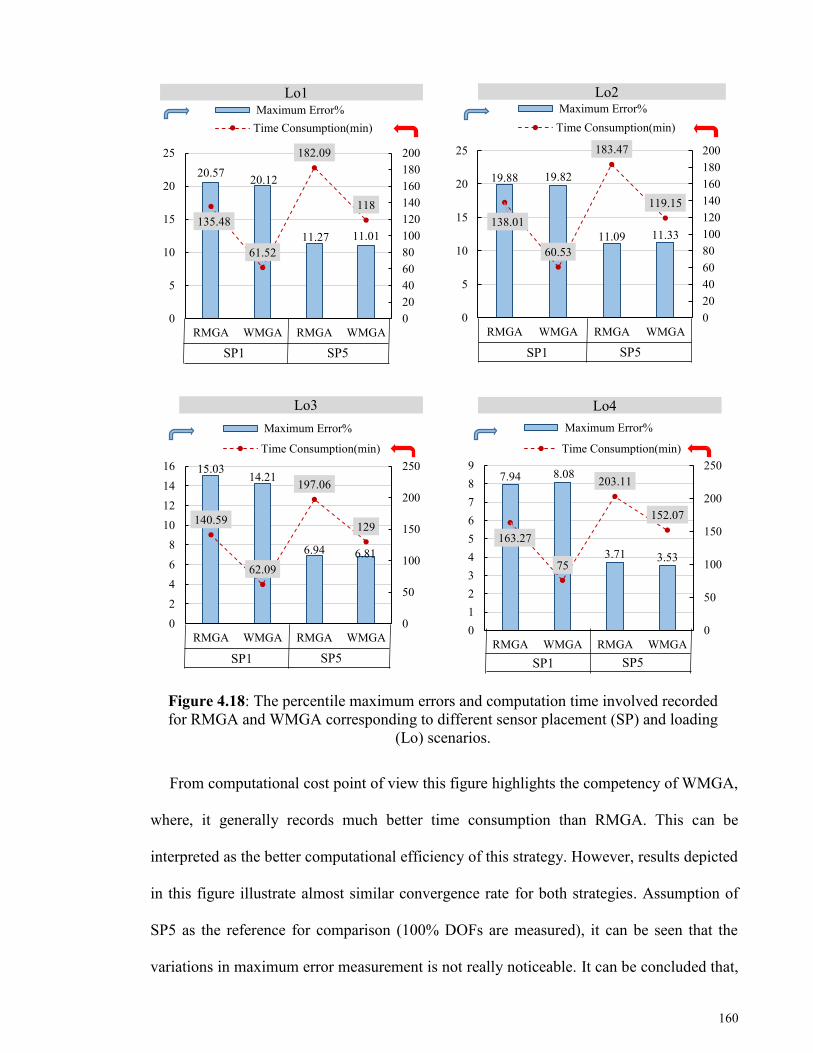
160

Figure 4.18: The percentile maximum errors and computation time involved recorded

for RMGA and WMGA corresponding to different sensor placement (SP) and loading

(Lo) scenarios.

From computational cost point of view this figure highlights the competency of WMGA,

where, it generally records much better time consumption than RMGA. This can be

interpreted as the better computational efficiency of this strategy. However, results depicted

in this figure illustrate almost similar convergence rate for both strategies. Assumption of

SP5 as the reference for comparison (100% DOFs are measured), it can be seen that the

variations in maximum error measurement is not really noticeable. It can be concluded that,

20.5720.12

11.27 11.01

135.48

61.52

182.09

118

0

20

40

60

80

100

120

140

160

180

200

0

5

10

15

20

25

RMGA WMGA RMGA WMGA

Maximum Error%


19.88 19.82

11.09 11.33138.01

60.53

183.47

119.15

0

20

40

60

80

100

120

140

160

180

200

0

5

10

15

20

25

RMGA WMGA RMGA WMGA

Maximum Error%


15.0314.21

6.94 6.81

140.59

62.09

197.06

129

0

50

100

150

200

250

0

2

4

6

8

10

12

14

16

RMGA WMGA RMGA WMGA

Maximum Error%


7.94 8.08

3.71 3.53

163.27

75

203.11

152.07

0

50

100

150

200

250

0

1

2

3

4

5

6

7

8

9

RMGA WMGA RMGA WMGA

Maximum Error%


Lo1

SP5 SP1

Lo2

Lo3 Lo4

SP5 SP1 SP5 SP1

SP5 SP1

161

from the view of the convergence rate in only structural identification (and not damage

detection) RMGA can compete with WMGA. Eventually, to assess the applicability and

effectiveness of WMGA for damage detection of large-scaled structures, two damage

scenarios (DS) have been proposed as tabulated in Table 4.13. It is observed that, damage is

imposed on only 3 of 196 elements (about 1.5%) and 3% of all elements due to DS1 and

DS2, respectively. Moreover, DS1 is proposed on elements placed at the northern and the

left-hand panel zone, while, elements of DS2 are distributed in the whole structure.

Table 4.13: Damage scenarios (DS) imposed to the 3D truss shown in Figure 4.17.

DS First

node Element

End

node

Reduction

(%) Top/Bottom/Diag. Off/On

DS1

36 68 52 30 Bottom (N,L) Off

20 33 49 25 Top (N,L) Off

13 29 53 20 Diag. (N,L) On

DS2

35 46 50 25 Bottom (N,L) On

22 37 55 25 Top (S,R) Off

12 14 17 20 Diag. (N,R) Off

34 47 48 20 Diag. (S,R) On

5 8 10 30 Top (N,R) On

21 39 45 30 Bottom (S,L) Off

Note: Reduction in stiffness (%) represents the magnitude of damage; north (N) and

left (L) imply the position of panel zone in structure.

In addition, sensor placement scenarios (SP) that previously utilized for identification are

tabulated in Table 4.14 corresponding to DS1 and DS2 for damage detection. Finally, damage

detection is carried out for considered large-scaled structure by implementing WMGA

(known mass). It should be pointed out that, there are several sub-structure techniques

available to effectively analysis this system. In this study, reduction of the size of

162

characteristic’s matrices (i.e., stiffness, mass and damping) is governed by the sensor

placement scenarios (measured and omitted DOFs), initially. Later, damage detection

strategy proceeds, and by fixing identified parameters for undamaged members, the size of

matrices is progressively reduced. To overcome the issue of false detection, a higher safety

factor (threshold) is presumed to distinguish damaged and undamaged members. The

identification and damage detection strategy are run 5 times and the percentile value of

success in detecting location as well as the magnitude of damages are comparatively

described in Figure 4.19 with respect to the various loading (Lo) and damage scenarios (DS).

Table 4.14: Sensor placement (SP) scenarios utilized for identification and damage

detection of Example 4.6.3.

DS SP Panel zone

𝑇𝐿𝑁 𝑇𝑅

𝑁 𝑇𝐿𝑆 𝑇𝑅

𝑆 𝐵𝐿𝑁 𝐵𝑅

𝑁 𝐵𝐿𝑆 𝐵𝑅

𝑆

Node number (X, Y and Z)

DS1

SP1 1,20,53 10,17,26 7,8,

22

16,48,

56

13,24,

50

6,12,

32

14,44,

46

11,27,

54

SP2

1,3,19,

20,29,

30,49,53

10,15,17 2,8 56

9,13,

24,

35,50

32,6,

28 21 27

DS2

SP3 1,49,53 10,15,17 7,8,

22

16,48,

56

13,24,

50

6,12,

32

14,44,

46

27,34,

54

SP4 19,20,29 4,30,53 2,8,

23

22,48,

55

9,13,

35

12,28,

32

21,45,

46

11,34,

54

DS1,

DS2 SP5 Full measurement

Note: 𝑇𝑅𝑁 represents the top (T) northern (N) and right-hand panel, 𝐵𝐿

𝑆: the bottom (B)

southern (S) and left (L) side panel, DS: damage scenario and SP: sensor placement

scenario.

163

In overall, it is observed that the detection of magnitude and especially location of damage

for online scenarios are remarkably successful. For instance, in Figure 4.19 (a) and (b) in the

cases where Lo1 (in view of 10% noise imposed) is applied on SP1-SP4 the satisfactorily

high success is recorded for online damages. This arises from the fact that the optimum

evaluation of the time-history of jerk considerably improves the proposed value of fitness for

damages those were imposed online. In addition, Figure 4.19 shows much adequate success

in detection of diagonal members rather than that of horizontal members on top or bottom

layer. Consequently, the superiority of WMGA for damage detection is demonstrated in this

figure, where 80% success in detecting the location and 60 % success in detecting the

magnitude of damage for about 3% members are achieved by the measurement of only 20%

DOFs of such large-scaled structures.

4.7 Chapter summary

In this Chapter, the wavelet-based strategy introduced in Chapter 3 for structural simulation was

extended for structural identification and damage detection using enhanced genetic

algorithms. An optimum operation was presented for sensitivity analysis of accelerations

capable of using different basis functions (namely, jerk analysis), initially. It was shown that,

the proposed operation of derivative is very sensitive to small changes of accelerations even

selecting considerably small sampling rates (long time intervals). It was confirmed that,

because of the property of unconditional stability, from the computational efficiency point of

view the fitness evaluation is significantly improved by using the longer time intervals. The

emphasis was on the precisely capturing broad frequency contents with adaptive collocation

points of wavelets.

164

Figure 4.19: Damage detection success % (location and magnitude) using WMGA for different sensor placements (SP), loadings

(Lo) and damage scenarios (DS); (a) DS1, (b) DS2, (c) DS2 (presented in Tables 4.13 and 4.14).

0

50

100

0

50

100

T B

Dia

g.

Off

On T B

Dia

g.

Off

On T B

Dia

g.

Off

On T B

Dia

g.

Off

On T B

Dia

g.

Off

On T B

Dia

g.

Off

On T B

Dia

g.

Off

On T B

Dia

g.

Off

On

Detection Success % (Location) Detection Success % (Magnitude)

0

20

40

60

80

0

50

100

T B

Dia

g.

Off

On T B

Dia

g.

Off

On T B

Dia

g.

Off

On T B

Dia

g.

Off

On T B

Dia

g.

Off

On T B

Dia

g.

Off

On T B

Dia

g.

Off

On T B

Dia

g.

Off

On


0

50

100

0

50

100

T B Diag. Off On T B Diag. Off On T B Diag. Off On T B Diag. Off On


(a)

SP2 SP1 SP2 SP1 SP2 SP1 SP2 SP1

Lo1 Lo2 Lo3 Lo4

(c)

Lo1 Lo2 Lo3 Lo4

SP5 SP5 SP5 SP5

SP3 SP4 SP3 SP4 SP3 SP4 SP3 SP4

Lo3 Lo1 Lo2 Lo4

(b)

165

Later, the wavelet-based scheme was implemented through a modified GA-strategy for

structural identification and damage detection. In this regard, the fitness evaluation (known

as the core of GA) was developed toward the most optimum strategy. As a consequence, a

combined multi-species GA was adopted through a compatible search space reduction

algorithm (SSRM) suitable for large-scaled structural identification to identify unknown

stiffness, mass and damping ratios. In addition, a predictor/corrector approach was proposed

for output-only identification using WMGA strategy in time domain. The strategy works by

simultaneously calculating the input forces as the structural parameters (stiffness and

damping) were identified.

Eventually, the proposed evolutionary process was extended to the structural damage

detection through a progressive calibrating algorithm. The analysis of convergence and

computational efficiency were introduced as the necessary and sufficient criterions to

evaluate evolutionary procedures. Accordingly, the convergence rate of the proposed strategy

was examined on three numerical applications. It was inferred that, the GA-based exploration

and exploitation phases are optimally satisfied by the used of improved SSRM, and therefore

a great convergence rate is accomplished. In addition, the lesser effect of I/O noise to the

signal were recorded for the proposed WMGA.

On the other hand, computational cost (time taken to solve the problems) was investigated

in the view of computational competency. It was concluded that, especially for large-scaled

structures the identification of numerous unknowns is optimally achieved by the remarkably

lesser computation time involved and resulting the very cost-effective strategy compared

with existing algorithms. Damage detection was conducted and results demonstrated the

superiority of the proposed method especially for online scenarios. It was also shown that,

the proposed method gave the minimum false detection for online imposed damages, where

the jerk evaluation gained the much better indication of damage rather than acceleration

166

itself. Consequently, the proposed algorithm can be considered as a sufficiently reliable

strategy especially for long time identification and online assessment of large-scaled

structures.

167

CHAPTER 5: EXPERIMENTAL VERIFICATION

5.1 Introduction

In order to investigate the effectiveness and capability of the proposed structural

identification and damage detection strategies in Chapter 4 on more realistic data, three

structural models have been constructed and tested in the laboratory for different scenarios

of loading and damages. The first experiment involves the output-only identification of a four

story MDOF system. The aforesaid system is designed with rigid beams (provided by rigid

Plexiglas) and relatively flexible aluminum columns (thin aluminum columns) in order to

invoke shear building behavior. The structure is subjected to base excitation and the force

identification is also considered along with identification of stiffness values and damping

parameters. The second structure is also a four story shear building constructed with thick

aluminum columns and rigid beams. This MDOF system is subjected to different nodal

excitations, and structural identification of known and unknown mass systems is considered

on intact structure first. Later, the damage detection strategy proposed in Chapter 4 is

conducted to detect the location and the magnitude of damages imposed to the structure.

Eventually, the third experiment involves a 2D steel and pin-jointed truss designed with

rectangle hollow sections as horizontal and vertical elements and double strips used for

diagonal members. The structural identification and damage detection of this system are

considered for different scenarios. Accordingly, for the last two experiments I/O data

measurements are available. As there is no online damage induced to the structures, the only

first term of Equation (4.21) is considered for fitness evaluations and the effect of jerk

evaluation is ignored. Finally, the results obtained from the experiments are presented and

discussed in subsequent sub-sections.

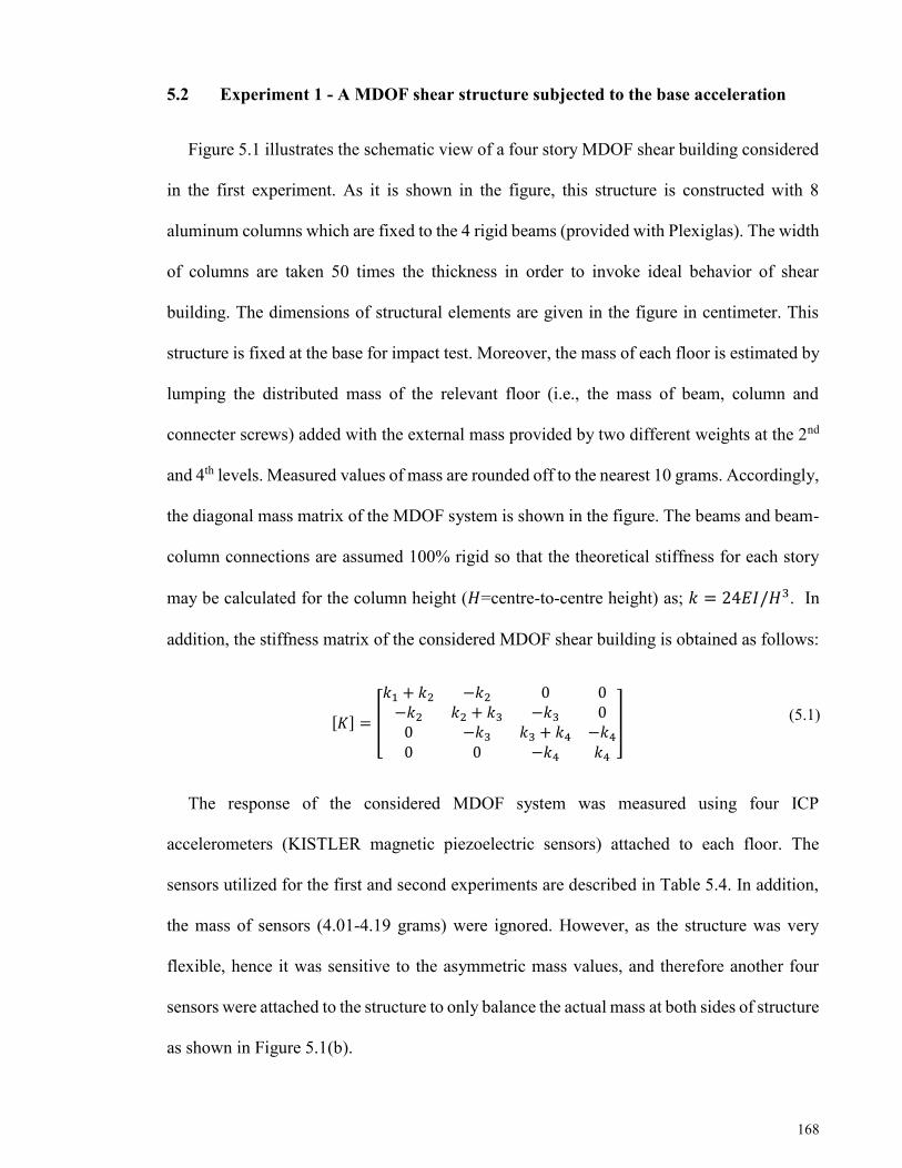
168

5.2 Experiment 1 - A MDOF shear structure subjected to the base acceleration

Figure 5.1 illustrates the schematic view of a four story MDOF shear building considered

in the first experiment. As it is shown in the figure, this structure is constructed with 8

aluminum columns which are fixed to the 4 rigid beams (provided with Plexiglas). The width

of columns are taken 50 times the thickness in order to invoke ideal behavior of shear

building. The dimensions of structural elements are given in the figure in centimeter. This

structure is fixed at the base for impact test. Moreover, the mass of each floor is estimated by

lumping the distributed mass of the relevant floor (i.e., the mass of beam, column and

connecter screws) added with the external mass provided by two different weights at the 2nd

and 4th levels. Measured values of mass are rounded off to the nearest 10 grams. Accordingly,

the diagonal mass matrix of the MDOF system is shown in the figure. The beams and beam-

column connections are assumed 100% rigid so that the theoretical stiffness for each story

may be calculated for the column height (𝐻=centre-to-centre height) as; 𝑘 = 24𝐸𝐼/𝐻3. In

addition, the stiffness matrix of the considered MDOF shear building is obtained as follows:

[𝐾] = [

𝑘1 + 𝑘2 −𝑘2 0 0−𝑘2 𝑘2 + 𝑘3 −𝑘3 00 −𝑘3 𝑘3 + 𝑘4 −𝑘40 0 −𝑘4 𝑘4

] (5.1)

The response of the considered MDOF system was measured using four ICP

accelerometers (KISTLER magnetic piezoelectric sensors) attached to each floor. The

sensors utilized for the first and second experiments are described in Table 5.4. In addition,

the mass of sensors (4.01-4.19 grams) were ignored. However, as the structure was very

flexible, hence it was sensitive to the asymmetric mass values, and therefore another four

sensors were attached to the structure to only balance the actual mass at both sides of structure

as shown in Figure 5.1(b).

169

Figure 5.1: The schematic view of test setup in lab for output-only identification of the

flexible MDOF shear system, (a) large shaking MDOF shear system at the base (S(t): base

acceleration), (b) fixed support at the base for impact test, (c) dimensions (cm).

(c)

6

t =

0.1

2

H =

17

𝒎𝟏

𝒎𝟒

Mass = diag (𝑚1 𝑚2 𝑚3 𝑚4) Mass = diag (0.29 2.32 0.29 1.22) kg

6

20

t =1.5

Aluminum columns

(b)

(a)

𝒎𝟐

𝒎𝟑

Plexiglas rigid story

S(t)

Shaking MDOF shear

structure at the base

Extra sensors only to

balance the weight at the

both sides

Measuring time-history

acceleration of the base

Extra mass to evaluate

the mass identification of

O-only data

Fixed support at the

base

170

For the purpose of output-only identification, this structure was fixed on a flexible MDOF

shear building shown in Figure 5.1(a). Subsequently, the time-history of acceleration S(t)

was measured at the top surface of the base structure and was assumed to be the records of

base excitation for the main experiment.

5.2.1 Preliminary measurements and calculations

As a reference for comparison of the calculated results, and in order to properly perform

the identification and therefore structural health monitoring tests, a set of preliminary tests

were first conducted. This sub-section contains static tests to predict the as-built stiffness of

the structure (static), as well as several impact tests to extract the as-built natural frequencies.

Taking 𝐸 as 69 GPa for the modulus of elasticity of the aluminum columns, the theoretical

stiffness value of 𝑘 =3455.09 N/m will be calculated for each story. As there was no

information available on the actual material and also the as-built stiffness of the considered

structure, static tests were conducted. The schematic view of static tests performed in the lab

is shown in Figure 5.2. As apparent in the figure, the first story of the considered system was

mounted horizontally to a fixed vertical support. Different weights were hung from the first

story while displacement transducer recorded the displacement. For this purpose, non-contact

laser sensor (KEYENCE; precision 0.01mm) was utilized to record the displacements due to

the different weights added.

171

Figure 5.2: The schematic view of static test performed in lab for the first MDOF

system (O-only identification).

Accordingly, the as-built stiffness of one story was determined from the slope of the

regression line obtained from different load-displacement points measured for several

different weights applied. In this regard, the stiffness value of 𝑘 =2421.18 N/m was

measured per story from the static tests. It was recognized that the difference between the

static and theoretical stiffness was noticeable. This could be due to the fact that the actual

material properties of considered structure were not available in lab. However, the stiffness

value obtained from the static tests was logically more accurate than that of the theoretical

values.

The impact tests were performed in order to compare stiffness values. Initially, the

structure was fixed to a rigid base as shown in Figure 5.1(b). Later, the considered MDOF

shear structure was excited by a hammer and the response recorded with sensors

Different weights

used as static load

Displacement

measurement

using non-

contact laser

sensor

The first story is

mounted horizontally

to a rigid support

Non-contact laser sensor (KEYENCE),

the precision is set to 0.01 mm.

172

(accelerometers) at each story using a 16 channel digital data analyzer (OROS36) at a

sampling rate of 2.048 kS/s. In addition, the structural frequencies were extracted by

implementing the fast Fourier transform (FFT) to convert the response signal from time

domain into the frequency domain (power spectrum of the signal). The natural frequencies

obtained from the solution of eigenvalue problems adopted for theoretical and static stiffness

values and those determined from the power spectrum of response are tabulated in Table 5.1

corresponding to the four modes of the MDOF system. It was observed that the response at

other levels and for other impacts, identified almost the same frequencies. However, data in

Table 5.1 correspond to the response at the 4th story due to impact at the same story.

Table 5.1: Calculated and measured natural frequencies of MDOF shear structure.

Theoretical stiffness =

3455.09 (N/m) per

story

Static stiffness =

2421.18 (N/m) per

story

Measured frequencies

from power spectrum

of response

f (Hz) Period (s) f (Hz) Period (s) f (Hz) Period (s)

Mode 1 3.12 0.32 2.61 0.38 2.59 0.38

Mode 2 7.85 0.13 6.57 0.15 6.55 0.15

Mode 3 24.81 0.04 20.77 0.05 20.72 0.05

Mode 4 25.83 0.039 21.63 0.046 21.08 0.047

Note: The mass is lumped at each story as shown in Figure 5.1 for all 3 cases considered.

Table 5.1 shows that, the natural frequencies extracted from the impact test and those

obtained from the static measurements were reasonably close. Consequently, the stiffness

value determined from static tests will be considered as the actual stiffness of the structural

elements and this should form the reference value of stiffness for further comparisons.

173

5.2.2 Main identification test

The main objective of this experiment is to evaluate the applicability and efficiency of

WMGA strategy proposed in previous chapter for structural identification problems when

output-only measurements are available. In other words, the stiffness and damping

parameters of each story are treated as unknown values to be identified while the

measurement of input forces is not available. The base structure was excited manually for 5

sec in the same direction with the attached MDOF shear building (Figure 5.1). As both

systems are supposed to be shear building structures, it is reasonable to transfer the

acceleration at the base structure (shaking MDOF system) to the dynamic equilibrium

governing the top structure in order to determine the actual forces. The response of the top

MDOF structure as well as the base acceleration were measured using five ICP

accelerometers (KISTLER magnetic piezoelectric sensors) attached to the base and each

story, respectively. The measured data of accelerometers are then recorded using a 16 channel

digital data analyzer (OROS36) at a sampling rate of 5.128 kS/s. Despite the fact that, the

highest frequency of the structure is only 21.08 Hz (for the 4th mode), selecting such high

sampling frequency allows for a better capture of excitation and resulting in a more precise

simulation of the response during identification. Finally, WMGA parameters utilized for

structural identification of this experiment are given in Table 5.2. It should be emphasized

here that the fairly broad range of 2.2 and 0.4 times actual values is selected as the search

limits of unknown stiffness. In addition, the search limits of damping parameters

corresponding to the first two modes are set as 0 to 3 for α and 0 to 0.0002 for β.

174

Table 5.2: WMGA parameters utilized for force identification (Experiment 1).

Known mass

Pop-size 5×30 Runs 3

Generations 3×100 Conducted SSRM after 100

Crossover rate 0.6

Mutation rate 0.2

Periodic migration (z1,z2) 5, 0.1-0.2

Window width 4

Regeneration 3

Reintroduction 80




5.2.3 Results and discussion

Figure 5.3 illustrates the first 4000 points of acceleration time-histories recorded for

corresponding nodes at a sampling rate of 5.128 kS/s. It should be pointed out that, complete

data measurement is considered for this experiment. In addition, as this experiment involves

force identification, a known mass problem is considered. As shown in Figure 5.3(e), the

maximum effect of noise was observed for the recorded accelerations at the base (designated

by S(t)). However, the noise effect was gradually reduced for the higher levels of the

considered MDOF shear system. The reason for this comes from the fact that the main

excitation was applied to the base manually as an ambient excitation with the highest signal-

to-noise ratio.

175

Figure 5.3: Time-history of acceleration (the first 4000 points) corresponding to, (a)

story 4, (b) story 3, (c) story 2, (d) story 1, (e) S(t): the base acceleration (g = 9.81

m/sec2).

Therefore, the uncontrolled excitation to the unknown base structure causes the larger

effects of the signal-to-noise. The structural identification is conducted using WMGA

parameters presented in Table 5.2. The time-history of identified force for 250 measured data

0 500 1000 1500 2000 2500 3000 3500 4000-0.08

-0.06

-0.04

-0.02

0

0.02

0.04

0.06

0.08DOF NUM-4

0 500 1000 1500 2000 2500 3000 3500 4000-0.08

-0.06

-0.04

-0.02

0

0.02

0.04

0.06

0.08DOF NUM-3

0 500 1000 1500 2000 2500 3000 3500 4000

-0.04

-0.03

-0.02

-0.01

0

0.01

0.02

0.03

0.04

Base

0 500 1000 1500 2000 2500 3000 3500 4000

-0.04

-0.03

-0.02

-0.01

0

0.01

0.02

0.03

0.04

DOF NUM-2

0 500 1000 1500 2000 2500 3000 3500 4000

-0.04

-0.03

-0.02

-0.01

0

0.01

0.02

0.03

0.04

DOF NUM-1

500

(e)

(d)

(c)

(b)

(a)

A

ccel

erat

ion

(g)

Acc

eler

atio

n (

g)

Acc

eler

atio

n (

g)

Acc

eler

atio

n (

g)

0.01

0.02

0.03

0.04

-0.04

-0.03

-0.02

-0.01

0.01

0.02

0.03

0.04

-0.04

-0.03

-0.02

-0.01

0.01

0.02

0.03

0.04

-0.04

-0.03

-0.02

-0.01

-0.08

-0.06

-0.04

0.04

0.06

0.08

4000

3500

3000

2500

2000

1500

1000

0

-0.08

-0.06

-0.04

0.04

0.06

0.08

A

ccel

erat

ion (

g)

0

0

0

0

0

176

(between 500-750 acquired points) corresponding to the second and third levels is plotted in

Figure 5.4.

Figure 5.4: Time-history of identified force (500 to 750 acquired points)

corresponding to, (a) story 2, (b) story 3.

The actual forces for each level were obtained by multiplying the base acceleration S(t) to

the actual mass at each level in inverse direction. As shown in Figure 5.4, the proposed

WMGA force identification strategy acts as a filtering procedure in order to reduce the effect

of noise. This is most likely due to the various scales of adaptive wavelet functions and

relatively compatible collocation points utilized for capturing the response of structure. It is

demonstrated that even with high signal-to-noise ratio data, the force identification is

reasonably reliable for ambient excitation done manually. It should be emphasized here that,

in order to implement the proposed procedure of force identification the first underlying

presumption is that the structure should be at rest condition. Providing such ideal condition

for this test was either impossible or very difficult. Undoubtedly, the aforementioned

0 50 100 150 200 250-0.2

-0.1

0

0.1

0.2

0.3

0.4

0.5

0 50 100 150 200 250-0.02

-0.01

0

0.01

0.02

0.03

0.04

0.05

0.06

Fo

rce

(N)

0

0.1

0. 2

0. 3

0. 4

-0.2

-0.1

750

700

650

600

550

500

Forc

e (N

)

500

550

600

650

700

750

(a)

Identified Force

Actual Force

(b)

Identified Force

Actual Force

0. 4

-0.2

-0.1

0

0.1

0.2

0.3

0.5

177

difficulty causes errors in identification procedure. Furthermore, this figure shows more

noticeable errors recorded for identified force at the third level rather than the second one.

This probably is because of the very light mass at this level in the vicinity of two heavy

masses corresponding to the second and fourth levels.

Figure 5.5: The percentile total average error of identified force and the mean error

(%) in identified stiffness of each story for output-only measurement.

Subsequently, by considering the initial stiffness values obtained from the static test, the

percentile total average error computed for identified force (at 5 sec of excitation) and the

percentile mean error in identified values of stiffness corresponding to each level of MDOF

system are comparatively plotted in Figure 5.5. This figure demonstrates acceptable

identified values for stiffness. For instance, about 6.7%, 4.3% and 8.6% of mean error were

recorded for identified stiffness values of level 1, 2 and 4, respectively. In contrast, the

highest error of 15.8% was measured for the identified value of stiffness corresponding to

level 3. This results are in the agreement with the results shown in Figure 5.4, where the

maximum differences are observed for the identified force at level three compared with the

second or other levels. Moreover, the percentile total average errors obtained for four

6.734.27

15.08

8.64

53.07

35.25

65.22

41.88

0

10

20

30

40

50

60

70

0

5

10

15

20

Story 1 Story 2 Story 3 Story 4

Mean Error in Identified Stiffness (%)

Total Average Error of Identified Force (%)

Mea

n E

rror

in I

den

tifi

ed

Sti

ffnes

s (%

)

To

tal Averag

e Erro

r of

Iden

tified F

orce (%

)

178

identified forces demonstrate the average error of about 48.8% for all levels. This value seems

undesirable compared to the very accurate numerical results achieved in Chapter 4 for force

identification. This probably arises from two factors. Firstly, the ambient excitation applied

to the base is an unrealistically irregular one, while it could be applied with an actual

instrument in order to be controlled in particular ranges of frequencies or amplitudes.

Secondly, the effect of high signal-to-noise ratio was not considered in Chapter 4 for force

identification (especially for irregular distribution of mass at different levels) to accomplish

the precise results. Furthermore, the effect of rest condition may be another source of error

measurements. Overall, the structural identification results demonstrate that the proposed

strategy for output-only data is a very good strategy, especially for real cases of irregular

ambient data. However, it could be perfected by proper planning in identification. It is very

important to keep in mind that, one of the main source of errors observed in Figure 5.5 is the

assumption of lumped mass matrix for structural modeling in this real case. Undoubtedly,

aforesaid assumption diversely affects the identified stiffness values, especially for ambient

vibration data.

5.3 Experiment 2 - A MDOF shear structure under nodal excitation

The schematic view of the test setup performed in lab for the second experiment is

illustrated in Figure 5.6. The MDOF shear system considered for this experiment was

constructed with 8 thick columns (provided with aluminum) and 4 rigid beams (provided

with Plexiglas). The width of columns are taken 12 times the thickness and allows for the

assumption of the shear behavior of the MDOF system (existing for only one DOF per story).

This structure is fixed at the bottom for impact and the main structural health monitoring

tests. Moreover, the mass of each floor is estimated by lumping the distributed mass of the

179

corresponding story (i.e., the measured mass of beam, column and connecter screws) added

with the external mass provided by two different weights at the 2nd and 4th levels. Measured

values of the mass are rounded off to the nearest 10 grams and the diagonal mass matrix of

this system is shown in the figure. In addition, in this experiment the mass of four

accelerometers attached to structure is ignored. The beams and beam-column connections

are assumed 100% rigid. Therefore, stiffness matrix of the system is obtained from Equation

(5.1).

Figure 5.6: The schematic view of the test setup: (a) the laboratory aluminum MDOF

shear building, (b) dimensions of the frame (m), (c) dimensions of the columns (m),

(d) dimensions of the rigid beam (m).

Mass = diag (𝑚1 𝑚2 𝑚3 𝑚4) Mass = diag (0.39 2.42 0.39 1.33) kg

(a)

4

× 0

.085

Story 1, DOF 1

Story 2, DOF 2

Story 3, DOF 3

Story 4, DOF 4

(b)

(c)

H =

0.1

t

= 0

.005

0.06

0.0

6

t =0.015

0.2

(d)

𝒎𝟏

𝒎𝟐

𝒎𝟑

𝒎𝟒

Extra mass =2.03 kg

Extra mass =1.02 kg

0.2

180

Accordingly, structural health monitoring of this structure is considered using the

proposed WMGA strategy in the previous chapter. To examine the performance of the

strategy, WMGA is conducted for structural identification of intact structure, initially. Later,

two different magnitudes of damage and locations are utilized in order to evaluate the

efficiency and capability of the proposed strategy for damage detection.


Stiffness estimation

As a basis for comparison of the obtained results, and to properly perform the

identification and therefore structural health monitoring tests, a set of preliminary tests were

first conducted. This sub-section contains static tests in order to predict the as-built stiffness

of the MDOF shear structure, as well as several impact tests to extract the as-built natural

frequencies.

Taking 𝐸 = 69 GPa for the modulus of elasticity of the aluminum columns, the theoretical

stiffness value of 𝑘 =1820.15 kN/m will be calculated for each story. As there was no

information available on the actual material and also the as-built stiffness of the considered

structure, static tests were conducted. The schematic view of static tests conducted in the lab

is illustrated in Figure 5.7. The first story of the considered system was mounted horizontally

to a fixed vertical support. Different weights were hung from the first story while

displacements were measured by displacement micrometer (precision 0.01 mm).

Subsequently, the as-built stiffness of one story was obtained from the slope of the

regression line determined from the different load-displacement points measured for several

different weights applied. The stiffness value of 𝑘 =1203.46 kN/m was measured per story

from the static tests. It was seen that the difference between the static and theoretical stiffness

181

was about 617 kN/m. Subsequently, the impact tests were performed to compare stiffness

values and select the reference value of stiffness.

Figure 5.7: The schematic view of static test conducted in lab.

As in the previous experiment, the MDOF shear structure was fixed to a rigid base and it

was excited by a hammer and the response recorded with sensors (accelerometers) at each

story using a 16 channel digital data analyzer (OROS36) at a sampling rate of 2.048 kS/s.

Accordingly, the FFT algorithm was then utilized to convert the response signal from time

domain to the frequency domain and the natural frequencies were determined from the plot

of power spectrum as illustrated in Figure 5.8 for one of the examples. It should be noted

that, a frequency band width of 1024, and therefore 2048 data points were utilized for the

FFT. Thus, the accuracy of measured frequencies was approximately ±0.5 Hz. Figure 5.8

Displacement measurement

(precision = 0.01mm)

The first story is mounted

horizontally to a rigid

support

Different weights

used as static load

182

shows the power spectrum of the response at fourth story due to the impact at that story. It

was observed that the response at other stories and for other impacts, identified the same

frequencies.

Figure 5.8: Power spectrum of response at fourth story due to impact at that story.

The natural frequencies obtained from the solution of eigenvalue problems adopted for

theoretical and static stiffness values and those determined from the power spectrum of

response are tabulated in Table 5.3 corresponding to the four modes of the MDOF system.

Table 5.3: Calculated and measured natural frequencies of undamaged MDOF

shear structure.

Theoretical stiffness

= 1820.15 (kN/m) per

story

Static stiffness =

1203.46 (kN/m) per

story

Measured frequencies

from power spectrum

of response

f (Hz) Period (s) f (Hz) Period (s) f (Hz) Period (s)

Mode 1 69.39 0.0144 55.63 0.0179 54.37 0.018

Mode 2 175.25 0.0057 141.42 0.0070 145.09 0.0069

Mode 3 538.26 0.0019 398.95 0.0025 390.51 0.0025

Mode 4 561.85 0.0018 419.68 0.0023 429.93 0.0023

Note: The mass is lumped at each story as shown in Figure 5.6 for all 3 cases

considered.

0 100 200 300 400 5000

0.02

0.04

0.06

0.08

0.1

0.12

0.14

Frequency (Hz)

54.37 (Hz)

145.09 (Hz)

390.51 (Hz)

429.93 (Hz)

Mag

nit

ud

e

183

Data displayed in Table 5.3 shows the closeness of obtained frequencies from the impact

test with those calculated based on the stiffness determined from the static test. This table

shows that especially for the first two modes of the structure results are very close. As a

consequence, the stiffness value obtained from static tests will be considered as the actual

stiffness of the structure and this should form the base value of stiffness for further

comparison.

Damage scenarios

Two different magnitudes of damage and correspondingly two different locations are

utilized in order to evaluate the capability and performance of the strategy. As it is shown in

Figure 5.9, damage magnitudes are categorized as small and large while the locations differ

corresponding to different damage scenarios one to three (DS1-DS3) imposed to the different

stories.

Accordingly, DS1, DS2 and DS3 indicate damage scenarios when only small damage is

induced in story 4, only large damage induced in the first story and the combination of this

two scenarios, respectively. Controlled damage is created by cutting the columns at the

proposed locations. As shown in Figure 5.9, small damage is created as partial cuts near to

the beams (in order to be in an area of high bending), whereas large damage is formed by a

longer cut at the center of columns. It should be pointed out that, the small and large damages

are induced on both sides of the structure. In order to predict the reduction in stiffness due to

the small and large damages, three columns are numerically simulated in a finite element

(FEM) software (ABAQUS 1998). The FEM models of the intact columns as well as

damaged columns with one end fixed and the other one free are shown in Figure 5.9. Shell

elements are used to model all three cases. An arbitrary distributed force of 25 N/cm is

applied to the top free nodes in the perpendicular direction. For all three cases the resulting

displacements are compared with the result of intact column and the reduction in column

184

stiffness is presented as the damaged index in Figure 5.9. It is to be noted here that, the

reduction in story stiffness is the same as the expected reduction in column stiffness e.g.,

42.69% for small damage, as damages are symmetrically applied to the both columns in a

story.

Figure 5.9: Damage scenarios and relative finite element models to estimate

damage index (%), (a) undamaged column, (b) small damage, (c) large damage

(dimensions are given in cm).

(a)

(b)

(c)

t =

0.5

10

6

2.7

5

2

5

0.5

2

2

0.2

3

0.2

3

Intact Column

Used for undamaged

structure

Damage Index = 42.69%

Small damage used as

DS1 and DS3

Damage Index = 88.03%

Large damage used as

DS2 and DS3

(a)

(a)

(a)

(b)

(c)

Sto

ry 1

Sto

ry 2

Sto

ry 3

Sto

ry 4

Bas

e

185

5.3.2 Main identification and damage detection test

Excitation force

Basically, the proposed WMGA strategy requires integration of accelerations. Thus it is

prefered to utilize a regular and smooth random force for this test rather than a very irrigular

and complex one. In this regard, a random multi-sinusoidal loading of 50-500 cycle per

second (Hz) with random magnitude of [-20, 20] N is utilized at a sampling rate of 5.128

kS/s. Accordingly, the force described above is applied through a shaker by roving it at

different levels of the structure.

Test setup

Figures 5.10 and 5.11 illustrate the test setup utilized in lab and a schematic view of the

dynamic testing and data acquisition system, respectively. The excitation force was input to

a 16 channel digital data analyzer (OROS36) and the signal was then passed through a power

amplifier in order to produce sufficient power for the electromagnetic shaker. The force

generated by the shaker was transferred to the structure and an ICP force sensor measured

the applied force (the specification of force sensor is presented in Table 5.4). The force

transducer (shaker) placement as well as the shaker-sensor-structure connection are shown

in Figures 5.10(a) and 5.10(b), respectively. The response of MDOF system to 10 sec of

excitation was measured by 4 ICP accelerometers (KISTLER magnetic piezoelectric sensors)

attached to each level of the MDOF structure. The classifications of sensors (accelerometers)

utilized are tabulated in Table 5.4. The signals measured by force sensor and accelerometers

are recorded by a 16 channel digital data analyzer (OROS36) at a sampling rate of 5.128 kS/s.

In addition, only the first 5 sec of response starting from just before the application of the

force are selected and copied to the input file for the damage detection program.

186

Figure 5.10: Test setup and instruments used in lab, (a) main test setup, (b) shaker

installation, top view, (c) accelerometer installation, side view.

Figure 5.11: The schematic diagram of data acquisition and test setup.

Fixed

accelerometers

Digital analyzer

(OROS)

Power amplifier

Roving shaker

Force

transducer

Data acquisition

(laptop)

OROS36-16 Channel

digital data analyzer

Laptop for data acquisition

Power amplifier

Shaker

Aluminum MDOF

shear system

Rigid support

Accelerometers

Rigid floor

Force sensor

Shaker (force

transducer)

Accelerometer

(KISTLER piezoelectric

sensors)

(a)

(b)

(c)

187

Table 5.4: The specification of accelerometers and force transducer.

Story Transducer Sensitivity

Range peak

(acceleration or

force)

1 Acceleration 103.9 m(V)/(g) 96 g

2 Acceleration 106 m(V)/(g) 94.3 g



1_4 Force 11.241 m(V)/(N) 890 N

Note: The gravity acceleration (g) = 9.81 m/sec2.

Accordingly, WMGA parameters utilized for the identification of intact structure and

damage detection are displayed in Table 5.5. In addition, half and twice the measured static

stiffness and mass values are used as the initial search limits of stiffness and mass,

respectively. The search limits of damping parameters corresponding to the first two modes

are set as 0 to 3 for α and 0 to 0.0002 for β.

Table 5.5: WMGA parameters utilized for Experiment 2.

Undamaged

Structure (unknown

mass)

Damaged

Structure (known mass)

Pop-size 5×50 5×30

Runs 3 3

Generations 3×180 3×100 Conducted SSRM after 180 100



Periodic migration (z1,z2) 5, 0.1-0.2 5, 0.1-0.2

Window width 4 4

Regeneration 3 3





188


Accordingly, for structural damage detection, the unknown mass problem is first

considered for initial structural identification. Later the identified mass from the initial step

is fixed as the known mass at each level corresponding to each DOF of structure. As it was

proposed before, the identified mass values are set as fixed values for all individuals (for

known mass problems) while the identified stiffness values are set as the initial predictions

of the first individual of species one and as the half of species 4 and 6 for local searches. This

resulted in a desirable calibration of the dynamic model using precise initial values.

Furthermore, the initial (reference) mass values were measured while the initial (reference)

stiffness values were obtained from the static tests.

Subsequently, identification of intact MDOF system is first performed in order to perceive

the changes in the identified values from those estimated from static tests or measurements.

The search limits are set as the half and twice the actual values. For instance, the search limits

of mass are set as [0.2-0.78], [1.21-4.84], [0.2-0.78] and [0.67-2.66] kg for the 1st, 2nd, 3rd

and 4th levels, respectively.

From our preliminary tests, it was concluded that the dynamic model does not perfectly

present the structural system, and that the first step of identification in the damage detection

serves to calibrate the model so damage can be precisely detected. In addition, it was included

that, for tests applying a same force input (in referring to the same frequency content and the

same amplitude bandwidth) at a same location, the strategy were consistently achieving better

detection results rather than applying different forces at different locations for identification

step and damage detection stage. For this reason, the same force as presented in previous

chapter is applied for both structural identification and damage detection at the last level of

MDOF system.

189

For comparison purpose, the modified genetic algorithm composed of 6 species proposed

in Chapter 4 (designated by MGA) is also adopted for structural identification of current

experiment. Accordingly, the well-known average acceleration of Newmark-β method is

performed for fitness evaluations of MGA at a sampling rate of 2000 S/s (time step of 0.0005

sec) for 10 sec of measured response at a sampling rate of 5.128 kS/s. The percentile total

average errors and corresponding CPU time consumption for stiffness identification of

undamaged structure regarding to the known and unknown mass problems are comparatively

depicted in Figure 5.12 (complete measurement).

Figure 5.12: Total average error and computation time involved for stiffness

identification of undamaged MDOF system shown in Figure 5.6

(known/unknown mass problems and full measurement).

The first observation from Figure 5.12 lies on the computational efficiency of the proposed

WMGA method where the accurate identification results (in terms of error evaluation) were

obtained for known mass and unknown mass with less CPU time consumption. It can be seen

from the figure that the percentile average error reached about 4.33% for known mass

identification using MGA whereas for the same case it was about only 2.2% for WMGA.

14.74 13.02 4.33 2.19

41.13

25.58

34.09

14.26

0

10

20

30

40

50

0

5

10

15

MGA WMGA MGA WMGA


Tota

l A

ver

age

Err

or

(%)

Unknown mass

Known mass

Tim

e Consu

mptio

n (m

in)

190

However, the convergence rate of results (in terms of accuracy evaluation) after two

approaches is almost the same; the remarkable finding lies on the worst performance of MGA

by higher computation time involved. In addition, Figure 5.12 demonstrates the higher error

measurements for stiffness identification of unknown mass problems where ten unknown

parameters are considered to be identified and making the problem much more complicated.

It should be emphasized that one of the main source of errors in both cases may be the

assumption of lumped mass for real mass matrix of this structure and this resulted in

modelling errors.

Subsequently, the next stage is the damage detection of the considered MDOF system due

to the damage scenarios imposed to the structure as outlined in Tables 5.6 and 5.7. For this

purpose, the first 5 sec of measured response due to the same force applied at the last level

was utilized at the same sampling rate by using the given WMGA parameters in Table 5.5.

To assess the performance of strategy for incomplete measurements the damage detection is

then carried out for a limited numbers of measured responses of damaged structure (presented

as sensor placements). It should be pointed out that, the results of identification of undamaged

structure for complete measurements are set as starting values for damage detection program.

Two aspects of known mass and unknown mass problems are evaluated through the WMGA

strategy and represent known or unknown mass identification whereas damage detection is

only performed by fixing identified mass values as the actual mass. Moreover, success in

detection of damage magnitudes is plotted in Figure 5.13 corresponding to different damage

scenarios (presented in Table 5.6) and different sensor placement (measured DOFs).

191

Figure 5.13: Success in identified damage index for different damage scenarios,

known/unknown mass problems and incomplete measurement (DOFs represents

measured DOFs).

One of the observations indicates that, the false detection is inevitable for the use of such

probability based procedures as in the proposed WMGA strategy. In this regard, the program

of damage detection is repeated 5 times and the success in identified damage index due to

the different damage scenarios (DS) presented in Figure 5.13 refers to the best identified

value of damage index. Despite the fact that a special attempt is made to establish the best

WMGA parameters which are consistently producing the best results for each particular case,

it can be seen that the false detection is still probable. As shown in the figure, the most

promising result of about 98 % was obtained for damage scenario 2 (large damage at the first

level) where the measurements of DOFs 1 and 4 were considered for a known mass problem.

In contrast, only about 49% success was gained for the third damage scenario (both large and

small damages induced) regarding to the measurements of only DOFs 2 and 3.

In addition, the CPU time was 25.58 min for structural identification of undamaged

structure corresponding to an unknown mass problem using the presented WMGA

parameters at 10 sec of excitation. It should be kept in mind that the identification of intact

structure is in fact a calibration step and requires to be performed on undamaged structure

96.47 98.1192.04

79.26 78.41

63.18

88.37 91.7583.92

63.07

76.54

48.83

0

20

40

60

80

100

120

DS1 DS2 DS3 DS1 DS2 DS3 DS1 DS2 DS3 DS1 DS2 DS3

Su

cces

s in

Id

enti

fied

Dam

age

Ind

ex (

%)

Unknown mass

Known mass

DOFs 1, 4

DOFs 2, 3

DOFs 1, 4

DOFs 2, 3

192

once. As the recorded response due to the only 5 sec of excitation is considered for damaged

structure, CPU time reached the optimum and fast record of 5.33 min for damage detection

strategy (known mass problem) on an I-5 CPU, 3.2GHz personal computer. As a

consequence, damage detection strategy can be conducted on site several times if it is

essential to check for the damage.

Moreover, as it was mentioned earlier the planning in identification of undamaged

structure and then damage detection of damaged structure plays the underlying role in order

to achieve the best success in damage magnitudes and locations. It is recognized that, for

damage detection of damaged structures, applying the same input force at the same location

as was applied for identification of undamaged structures is really beneficial. In this

argument, the same input force refers to the same frequency content and amplitude domain

while the same location refers to the same DOFs. Accordingly, to evaluate the effects of

different excitation scenarios, damage detection of current MDOF shear structure is carried

out for two different procedures. In this regard, the identification of undamaged system is

first conducted using the considered multi-sinusoidal force at level four. Later, damage

detection strategy is performed for the cases that the force is applied at level four and that at

level 2.

Results are Tabulated in Tables 5.6 and 5.7 corresponding to applying input force at

different location of MDOF system for damage detection. As was mentioned before results

are obtained after 5 repeats of test. The noticeable observation lies on more false detections

of location of damages for the case that the input force was applied at different DOF (level 4

for identification and level 2 for damage detection). For instance, Table 5.7 illustrates that

the success in detection of location was only 3 times of 5 repeats for the third damage scenario

(DS) when the initial identification was performed for unknown mass problem. In contrast,

the detection of location was successful 4 times due to the same case in Table 5.6.

193

Table 5.6: Results of damage detection due to the same input force applied at the same location as for undamaged MDOF

system and full measurement (after 5 repeats).


Damage scenarios (DS) Ave. for

small

Ave. for

large Success (%)

Ave. for

small

Ave. for

large Success (%)

DS1: Small at story 4 43.91 _ 100 (5/5) 44.78 _ 80 (4/5)

DS2: Large at story 1 _ 88.37 100 (5/5) _ 85.04 80 (4/5)

DS3: Small at story 4 and

large at story 1 40.02 87.49 80 (4/5) 38.11 92.37 80 (4/5)

Note: Ave = average damage index (%) identified except false detections.

Table 5.7: Results of damage detection due to the same input force applied at the different location as for undamaged

MDOF system and full measurement (after 5 repeats).


Damage scenarios (DS) Ave. for

small

Ave. for

large Success (%)

Ave. for

small

Ave. for

large Success (%)

DS1: Small at story 4 49.06 _ 80 (4/5) 36.09 _ 60 (3/5)

DS2: Large at story 1 _ 83.77 80 (4/5) _ 93.15 80 (4/5)

DS3: Small at story 4 and

large at story 1 51.91 80.47 80 (4/5) 31.68 74.32 60 (3/5)

Note: Ave = average damage index (%) identified except false detections.

194

In addition, it can be clearly seen in Table 5.6 that the location detections were

satisfactorily successful, especially for the single damage imposed to the structure.

Comparing the results of location detection with that of the magnitude detection demonstrates

sufficiently reliable results for the proposed strategy. With reference to the damage indices

obtained from FEM modelling (about 42.7% for small damage and about 88% for large

damage), the data displayed in Table 5.6 shows the promising results of the proposed damage

detection strategy. Consequently, accuracy of results in Tables 5.6 and 5.7 suggests that for

damage detection employing the same input force gains considerably reliable results than

cases where different input forces are implemented.

5.4 Experiment 3 - A 2D truss structure under nodal excitation

Figure 5.14 shows the schematic view of test setup for Experiment 3. A 2D pin-jointed

truss structure is considered for this experiment. As illustrated in the figure, this structure is

constructed with nine horizontal and vertical bar elements (provided with steel hollow

sections) and four diagonal bar elements (provided with double steel strips). It is to be noted

that six stiffeners are utilized in order to stiffen the diagonal elements and preventing

buckling phenomena in these slim members. All truss elements are connected with 8 pin

connections so that they are free to rotate. The structure is fixed to a moment free support at

the left and to a roller support (moment free) placed at the right side. In addition, to limit the

nodal responses of the structure only in horizontal and vertical directions (namely, x and y

directions), 4 larger hollow sections (shown by lighter colour frame in the figure) are used to

fix the perpendicular degree of freedom (z direction). As shown in Figure 5.14, all pin joints

are supported in z direction so that it is reasonable to assume 2D behavior. The intact structure

comprise of 13 DOFs indicated by red arrows in the figure.

195

The mass of each structural element is measured and compared with theoretical mass

value calculated with the mass density of steel 7850 kg/m3 for member sizes shown in Figure

5.14. It is observed that the measured mass matches the theoretical mass to approximately ±

20 grams. Eventually, in order to calculate the effective length of the structural members, 2.4

cm (1.2 cm from each side) is deducted from actual axis-to-axis length of the horizontal and

vertical members due to the connector plate in the joint. The effective length of diagonal

members is the actual axis-to-axis of diagonals as they are directly connected to the pin joints.

It should be emphasized that, the width of hollow sections (in principle direction) is selected

to about two times of the height in order to ensure 2D behavior.


Stiffness estimation and structural natural frequencies

In order to estimate the stiffness of truss members and extract structural natural

frequencies to employ in the identification strategy, a finite element model of the considered

structure is modelled in ABAQUS. The FEM is constructed using 13 bar elements and 2

different cross sectional areas corresponding to horizontal, vertical and diagonal members.

The mass density of steel 7850 kg/m3 and modulus of elasticity of steel 𝐸 = 207 GPa are

used for the modeling. Furthermore, at this stage the diagonal members are modelled as only

couple strip and the effect of internal stiffeners is not considered.

196

Figure 5.14: The schematic view of the test setup for Experiment 3: (a) the laboratory 2D truss, (b) sensor placement, (c)

dimensions of the truss (cm), node and element numbering, (d) new nodes and elements for the progressive damage detection

strategy, (e) section details (cm).

A

B

65

4×55

2

1

2

3

4

5

6

7 8

3

1

4

5

6

7

8

9

10

11

12

13

y

x

x

y

9

10

y

x

x

x

y

2 6

A

B

1.9

3.7

t = 0.1

1.7

2

t = 0.25

Section A-A: Hollow section

Section B-B: Double steel strips

(a)

(b)

(d)

Roller or fixed support

Fixed support

Roller support

(c)

(e)

197

Figure 5.15: The first six mode shapes and natural frequencies obtained from FE

model of 2D truss structure.

The natural frequencies obtained from the software corresponding to the first 6 and 13

modes of the structure are displayed in Figure 5.15 and Table 5.8, respectively. As it is

displayed in Table 5.8 and Figure 5.15, the natural frequencies obtained from the FE model

of 2D truss varies from about 202 to 2120 Hz corresponding to the first and thirteen modes

of the structure. Moreover, impact tests were carried out to extract natural frequencies and

compare with those from the FE model. One of the clear results was obtained when a hammer

excited node 4 in y direction and the power spectrum of response at 4-y was taken using FFT

algorithm. The power spectrum of response is plotted in Figure 5.16.

Mode 6: 1198 (Hz)

Mode 5: 685.6 (Hz)

Mode 3: 519.3 (Hz)

Mode 4: 647.9 (Hz)

Mode 2: 355.2 (Hz)

Mode 1: 202.3 (Hz)

x

Y

198

Figure 5.16: Power spectrum of response at DOF 4-y due to impact at 4-y (shown in

Figure 5.14).

Table 5.8: Natural frequencies (Hz) obtained from FE model of 2D truss.

Mode

1 2 3 4 5 6 7 8 9 10 11 12 13

(Hz) 202 355 519 647 685 1198 1234 1397 1518 1588 1771 1823 2120

0 200 400 600 800 10000

0.01

0.02

0.03

0.04

0.05

0.06

Frequency HZ

FFT Power Spectrum Analysis

533 (Hz)

384.5 (Hz)

597 (Hz)

212.4 (Hz)

615 (Hz)

Mag

nit

ud

e

Frequency (Hz)

212.5 (Hz)

200 300 400 5000

2

4

6

8

10

12x 10

-3

Frequency HZ

FFT Power Spectrum Analysis

user

Typewriter

212.5 (Hz)

user

Oval

199

Due to the complexity of the structure, it was anticipated that the extracted natural

frequencies from the impact test are not obviously distinguishable. Especially, it is observed

that the natural frequencies corresponding to the higher modes cannot be detected. This is

most probably due to the local vibrations of structural elements, whereby they produced

significant energy in 1800-3000 Hz range and diminish at the higher structural frequencies.

It is very important to keep in mind that, in planning the identification experiments these

frequencies and relatively these modes are not excited. Accordingly, the peak points shown

in Figure 5.16 may be considered as the first five natural frequencies. However, the extracted

values of only the first two modes from the impact test are almost close to the obtained ones

from the FE model. In addition, it can be deduced from Figure 5.16, the major shortcoming

of the frequency domain procedures for structural identification, where the structural

frequencies corresponding to the higher modes cannot be detected in practical and real

structures. Consequently, the theoretical stiffness values are taken as the predicted ones and

assumed as the reference values for further comparison. The theoretical stiffness of elements

is calculated by E×Area/Length. It should be pointed out that, for each truss element the axial

rigidity (E×Area) is treated as unknown stiffness.

Damage scenarios

To evaluate the performance of the proposed damage detection strategy on a complex and

a larger scale structure, there are two damage magnitudes used at different locations of the

considered 2D truss experiment. The large damage magnitude is shown in Figure 5.17(a),

while Figure 5.17(b) shows the small one.

200

Figure 5.17: Damage scenarios imposed to the 2D truss, (a) large damage on element 4

shown in Figure 5.14, (b) small damage on element 12, (c) damage index obtained from

FE model (dimensions are given in cm).

Figure 5.17(a) illustrates the location and dimensions of the large damage. Different

damage scenarios (DS) are displayed in Table 5.10. It is seen that the large damage magnitude

is induced only for element 4. However, the small damage magnitudes are induced for

diagonal members. As shown in Figure 5.17, the small damage magnitude is formed by

removing one of the six internal stiffeners from the actual diagonal members. In order to

estimate the expected reduction in stiffness due to the large damage magnitude on element 4

and small damage magnitude on diagonal members the finite element analysis is conducted

using ABAQUS. For this purpose, firstly the whole element 4 (intact element) is modelled

6

1.9

10.25

26.5

Diagonals with six

internal stiffeners

Large damage

Small damage

84

5×12.8

(b)

(a)

Damage index (%) obtained from FE model:

Large damage imposed to the whole element 4 = 25.14.

Large damage imposed to half of element 4 = 67.85.

Small damage = 14.33.

(c)

53

201

in the software as one bar element (node 2 to node 4 shown in Figure 5.14) under +800 N

arbitrary axial force applied to node 4 (shown in Figure 5.14). The first model is considered

as the basis for further comparison. Secondly, element 4 is modelled using 3 bar elements,

involving a 10.25 cm bar from node 2 with the intact cross-sectional area, followed by the

next element (6 cm) as the damaged one with the reduced cross-sectional area and the last

being 36.75 cm intact bar element. The same axial force is then applied in order to compute

displacements. The resulting damage index is the expected reduction in stiffness of member

4 due to the large damage. The same procedure is performed to estimate the reduction in

stiffness of the new bar element (node 2 to node 9) due to the large damage in this element.

It is concluded that, when large damage is used for the whole element 4, the damage index is

estimated as 25.14%, while it is 67.85% when only half of element four is considered.

Accordingly, the FEM modeling is used to estimate the reduction in stiffness of diagonal

members due to the small damage (formed by cutting one of the stiffeners as shown in the

figure). Bar elements are utilized to model couple steel strips subjected to +500 N axial force.

A damage index of 14.33% was calculated for estimation of reduction in stiffness of

diagonals when one of the stiffeners is removed. As a consequence, the values obtained for

damage index corresponding to different damage scenarios are utilized to compare with the

identified values.

5.4.2 Main identification and damage detection test

Generally, there are many scenarios available in order to perform the main identification

and damage detection in this experiment. As this structure contains 8 nodes with 13

perpendicular DOFs, therefore planning for identification is the underlying step. The test

scenario described here refers to the one of the best scenarios, which was consistently

producing desirable results. In order to proceed for this experiment and recording the

202

response of the structure, complete measurement is considered. However, some of the results

for incomplete measurements are provided in Appendix E.

Excitation force

As mentioned earlier, the proposed WMGA strategy requires integration of accelerations.

Thus it is prefered to utilize a regular and smooth random force for this test rather than a very

irregular and complicated one. For this purpose, a random multi-sinusoidal loading of 150-

1800 cycle per second (Hz) with random magnitude of [-25,25] N is utilized for 15 sec at a

sampling rate of 5.128 kS/s. Accordingly, the force described above is applied by two shakers

in the vertical direction at node 4 placed at the center and horizontal direction at node 8 (free

DOF of the roller support) placed at the right side of the structure. In addition, a weight of

400 N is gradually hung to the node 5-y in 2 steps during 15 sec and is assumed as externally

constant load (shown in Figure 5.18). The constant load acts as a complementary force for

larger influence in response measurements. In other words, using such load helps to remove

the local vibrations of individual members and correspondingly higher frequencies which

most of the time appeared in terms of signal-to-noise. From our preliminary experiments, the

use of this load is worthwhile as the errors in measurements are significantly reduced.

However, it should be taken into account that, the use of a flexible basis i.e., very soft plastic

block is essential for applying the above mentioned incremental loads (constant load) in order

to damp the local vibration of the link member when applying the constant force.

Test setup

The excitation forces explained in previous section were input to a 16 channel digital data

analyzer (OROS36) and the signal was then passed through a power amplifier in order to

produce sufficient power for the electromagnetic shaker. The forces generated by the two

shakers were applied to the structure at node 4 in vertical direction as well as the horizontal

DOF of node 8 while two ICP force sensors measured the applied forces. The response of

203

2D truss structure to 15 sec of excitation was measured by 13 ICP accelerometers (KISTLER

magnetic piezoelectric sensors) attached to each DOF of the 2D truss structure i.e., 2-x, 2-y,

3-x,…8-x. The signals measured by force sensor and accelerometers are recorded by a 16

channel digital data analyzer (OROS36) at a sampling rate of 5.128 kS/s. In addition, only

the first 10 sec of response starting from just before the application of the force (constant

load equal to zero) are selected and copied to the input file for the damage detection program.

Actually, from the preliminary tests, the initial stiffness of diagonals was assumed as the

calculated axial rigidity due only to the double strips and the effect of stiffeners was not

considered. The identification was consistently giving a larger stiffness value for diagonals

which was constant for all intact diagonals. The results were predictable in presence of the

internal stiffeners. It should be kept in mind that, theoretically it is not possible to measure

or calculate the actual stiffness of diagonals due to the internal stiffeners. For this reason, the

identified stiffness value of intact diagonals including the internal stiffeners is set as the basis

for presenting the so-called damage index value. The procedure of damage detection is

carried out through four steps. The first step involving the structural identification of

undamaged structure. The second stage is identification of damaged structure and detecting

damaged members. In order to detect damaged members a threshold value of 5% is

considered. In this regard, the damage indices more than 5% indicated the presence of

damage in the member. It should be noted here that even for undamaged members, damage

index of 1 to 5% could be identified. Then the identified stiffness for undamaged members

is fixed for these members and the damage detection proceeds to the next step, progressively.

In addition, assumption of identified stiffness values as known parameters for progressive

steps allows the damage detection strategy to be applied to a broad range of complex and real

problems (such as this experiment). In fact, the aforementioned assumption resulted in

desirable calibration of the structural system. Calibrating the structural model simultaneously

204

with identification and damage detection provides a reasonably fair judgment for identified

stiffness values of members when there is no information on their actual values. Accordingly,

at the third step of analysis, based on the location of damage identified from the previous step

i.e., damages detected in elements 4 and 12 shown in Figure 5.14, adding extra nodes and

therefore extra accelerometers are required for the structure i.e., nodes 9 and 10. It is very

important to keep in mind that, even though the extra data are supposed to be acquired, the

current step is much simpler than previous ones as many unknown values have been already

identified and the number of unknowns is considerably reduced. It is seen that the program

automatically navigates user towards the location of damages. Subsequently, the last step is

conducted to finalize the locations and magnitude of damages. For this purpose, new

unknown stiffness values can be appended to the WMGA strategy due to the identified results

requiring reconsideration. However, for most of the cases the structural identification and

damage detection results obtained from the second step were sufficiently accurate and

reliable. It should be noted that, for the identification and damage detection in this experiment

it is assumed that the mass is known, since the mass of structure is not altered due to the

damages. Eventually, WMGA parameters utilized for this experiment are presented in Table

5.9 corresponding to the different steps of damage detection strategy.

Finally, half and twice the theoretical axial rigidity (E×Area) for each truss element is

used as the initial search limits of stiffness. The search limits of damping parameters

corresponding to the first two modes are set as 0 to 4 for α and 0 to 0.00001 for β.

205

Table 5.9: WMGA parameters utilized in Experiment 3.

Undamaged


Damaged


Step 1 Step 2 Step 3

Pop-size 5×40 5×40 5×30 5×20 Runs 3 3 3 3 Generations 3×120 3×120 3×90 3×50 Conducted SSRM after 120 120 90 50 Crossover rate 0.6 0.6 0.6 0.6 Mutation rate 0.2 0.2 0.2 0.2 Periodic migration (z1,z2) 5, 0.1-0.2 5, 0.1-0.2 5, 0.1-0.2 5, 0.1-0.2 Window width 4 4 4 4 Regeneration 3 3 3 3

Reintroduction 90 90 70 40




Table 5.10: Damage scenarios imposed to 2D truss shown in Figure 5.14.

Damage scenarios (DS)

Element No. DS1 DS2 DS3 DS4

4 Large _ Large Large

12 _ Small Small Small

1,5,9 _ _ _ Small


There are several possible scenarios in planning the structural identification and damage

detection of this system. The identification of this structure was first evaluated numerically

in order to accomplish the best strategy for identification. For this purpose, the considered

2D truss structure was simulated numerically for its actual geometry as well as boundary

conditions. One of the very important steps of the structural identification is to select the

characteristics of externally applied excitation(s) and its relative location to be applied in

206

order to achieve the maximum influence in the dynamic response of the structure. However,

care must be taken in considering the limitations of as-built structure for initial evaluations.

In other words, for initial assessments the available locations in real structure are considered

for applying input forces or sensor placements. From several available scenarios the best

results were consistently obtained for the case of two multi-sinusoidal input forces applied at

4-y and 8-x shown in Figure 5.18(a). Additionally, an incremental constant load is applied at

node 5-y. The detailed characteristics of input forces are discussed in previous section. The

locations of input forces (shaker placement) are shown in Figure 5.18(b). Accordingly, the

response of the considered system is numerically simulated using average acceleration of

Newmark-β approach for three input forces at a sampling rate of 5000 for 15 sec of excitation.

Complete measurements and the known mass problem are considered in order to process

both the numerical and experimental evaluations.

Figure 5.18: The schematic view of the test setup used for 2D truss, (a) the main layout

of the test, elements and nodes numbering, (b) loading scenarios.

Rigid supports to install

shakers

Shaker 1

Shaker 2

Incremental constant

loads

(a)

(b)

207

In order to highlight the robustness of the proposed WMGA strategy compared with

MGA, the fitness value histories of the first individual of each population (refers to the best

individual and thus the best results) during 360 generations are comparatively depicted in

Figure 5.19. For the purpose of a comprehensive comparison, the CPU time taken to proceed

each SSRM step is also presented.

Figure 5.19: Fitness value history of the best individual for 2D truss identification

(known mass), (a) the history of the best fitness value using WMGA and MGA,

(b) computational time (min) recorded at each SSRM step (full measurement).

Figure 5.19 illustrates the superior performance of WMGA strategy in both exploration

and exploitation phases of the genetic algorithms. It is shown that before employing the first

SSRM the accuracy of results obtained from the MGA is more than that of using Haar

wavelet. However, the time taken to process the exploration phase using Haar wavelet is

0 50 100 150 200 250 300 3500

100

200

300

400

500

600

700

800

900

1000

Total

(min)

Fit

nes

s V

alue

(unit

-les

s)

SSRM

SSRM

Generations

(a)

WMGA

MGA

CPU Time (min)

WMGA: 7.42 8.53 16.49 32.44

MGA: 17.05 18.42 16.60 52.07

(b)

Total:

208

considerably less than using MGA. It should be emphasized that, the sampling rate of 500

(sample point per second) was used for Haar wavelet (2M=2) compared with 2000 for MGA.

It is observed that there is a sharp increase in accuracy of results for WMGA after the first

SSRM step where 3D Legendre wavelets (2M=4) are used compared with MGA. In contrast,

the accuracy of simulated response obtained by MGA is gradually increased at this stage.

Subsequently, the precision of results in exploitation phase which basically involves the

search on global optima is excellent using the second kind of Chebyshev wavelet (2M=8) at

a sampling rate of 200. It can be concluded that, even by using larger sampling rates for

WMGA strategy, the entire frequency content of externally applied forces as well as wide-

band of natural frequencies of the structure are optimally captured, resulting in a very cost-

effective and reliable approach. For instance, the total CPU time of 32.44 min was recorded

on an I-5 CPU, 3.2GHz PC for used of WMGA whereas this value surged to about 52.07 min

for MGA.

Table 5.11: Damage scenarios imposed to 2D truss shown in Figure 5.17.

Damage scenarios (DS)

Element No. DS1 DS2 DS3 DS4

4 Large _ Large Large

12 _ Small Small Small

1,5,9 _ _ _ Small

Accordingly, the same scenarios of input force are applied to the current experiment for

structural identification and damage detection. Structural identification of undamaged system

is carried out assuming the known masses as those of measured one. In addition, the

theoretical stiffness values (axial rigidities) are taken as the initial and the reference values.

209

At this stage, only two cross-sectional areas of double strips were considered to estimate the

axial rigidity of diagonals. Therefore, identification program achieved larger stiffness values

for diagonals than the estimated. In referring to the presence of internal stiffeners, obtained

results were logical, however, there were no way to precisely estimate the actual stiffness of

diagonals. For this reason, in planning of identification and damage detection it was decided

to run the program of damage detection 2 or 3 times, progressively. In fact, the strategy acts

in calibrating the unknown stiffness values during the damage detection several times by

fixing the identified stiffness values as known parameters for subsequent steps. It is

anticipated that reliable detections will be achieved at the second or the third steps of strategy.

Accordingly, damage scenarios (DS) are used step-by-step and results of detections of both

damage locations and damage magnitudes are depicted in Figure 5.20 corresponding to 8

repeats of damage detection program.

Figure 5.20: Damage detection success % (location and magnitude) after 8 repeats

for different damage scenarios (DS) through two steps (full measurement).

Figure 5.20 demonstrates the excellent results for cases when a single magnitude of

damage is to be detected. However, for multiple damages the identified magnitudes and

95 71 86 65 83 59 98 87 94 77 87 71

10087.5

100

75

100

62.5

100 100 100 100 10087.5

0

20

40

60

80

100

120

0

20

40

60

80

100

120

Large Small Large Small Large Small Large Small Large Small Large Small

Detection Success % (Magnitude) Detection Success % (Location)

Det

ecti

on

Su

cces

s %

(M

agn

itu

de)

DS4

DS3

DS2

DS1

DS4

DS3

DS2

DS1

Second step

First step

Detectio

n S

uccess %

(Lo

cation

)

210

locations of large damages are sufficiently accurate. It can be seen from the figure that for

the cases of detection of a single small damage and a single large damage being considered,

success in location and magnitude is considerably less than cases when the same magnitude

of damages are to be detected. In other words, it can be concluded that the damage detection

is less satisfactory for multiple damages of different damage magnitudes. From several tests

conducted, it can be deduced that, the large damages often causes false detections on other

levels of damage. Consequently, detection of small damages will be somehow impossible

and the damage detection strategy has to be run again. In contrast, for the cases of a single or

multiple damages of similar magnitude being considered, the detection results are

exceptional. Finally, it should be emphasized here that one of the main source of error

detections is assumption of lumped mass for this 2D structure which in fact is not accurate

assumption for the real structural model. This diversely affects the response simulated

compared with response measured, resulting in the quality of the fitness evaluation.

5.5 Chapter summary

This chapter presented the experimental verification of the proposed WMGA strategy for

structural identification and damage detection of three real structures. For this purpose, some

of the promising results obtained from the experimental works were highlighted. Additional

results are given in Appendix E, accordingly. Basically, experimental evaluations are

necessary in presenting a realistic assessment of numerical aspects of structural health

monitoring approaches involving structural identification and damage detection strategies.

However, there is a lack of investigations on use of various structural models due to the much

greater difficulties for experimental evaluations rather than numerical studies.

Aforementioned experimental models were considered for structural identification of output-

211

only data as well as structural identification and damage detection of input/output measured

data. Force identification was carried out on a MDOF shear building subjected to base

excitation. It was shown that, even though the measurement of input forces was not available,

the accuracy of identified stiffness values was sufficiently acceptable. Subsequently, the

proposed strategy was performed for identification and damage detection of a MDOF shear

building and a 2D pin-jointed truss structure. The approach utilizes measurement and

identified values of undamaged structure in order to calibrate the structural model prior to

damage detection. This arises by fixing the identified mass of intact system for detection of

damaged structure. This provided considerably simpler and fast computations for damage

detection where it was considered as a known mass problem. In addition, the identified values

from identification of intact structure helped to initiate the search limits of damage detection

strategy to be the nearest values to the real ones.

It was shown that the modelling errors are reduced due to the calibration steps and it is

very important to use the same forces for both identification and damage detection strategies.

The damage detection results were impressive, especially when a single damage magnitude

is to be detected. For detection of damage scenarios involving large and small damages, the

modelling errors causes more false detections. It was observed that for these cases the large

damages are more easily detected rather than the small ones. It was demonstrated that by

using adaptive wavelet functions through an improved search limit reduction strategy, the

genetic algorithm phases are optimally proceeded, resulting in very cost-effective and

reasonably accurate results.

212

CHAPTER 6: CONCLUSIONS AND RECOMMENDATIONS

6.1 Introduction

The main findings of this research are presented in this chapter. These are categorized into

two main aspects. The first aspect involves the proposed wavelet-based method for structural

dynamics (forward analysis). Accordingly, the second aspect involves structural health

monitoring (inverse analysis) using the proposed wavelet-based method.

6.2 Structural simulation (forward analysis)

Numerical approaches are the only options for structural simulation because in most cases,

the applied excitations are not explicit functions. In addition, the technique for a solution of

general dynamic equilibrium can become very expensive for cases where a complex loading

is applied on large-scaled structures. It was presented that, orthogonal polynomials can be

widely implemented as a practical analysis of time dealing problems, particularly in the form

of wavelet analysis. It was emphasized that the obvious effectiveness from the property of

orthogonality is that the repeated components with similar characteristics are neglected in the

analytical process. Consequently, computational calculations are considerably reduced and

computation time involved is therefore decreased, hence the accuracy of responses will be

more desirable. One of the popular classifications of wavelet operators is originated from

orthogonal polynomials. It was recognized that, several attractive mathematical

characteristics of these wavelets such as efficient multi-scale decompositions, localization

properties in physical and wave-number spaces and fast wavelet transforms, have obtained

213

the practice of this efficient tool especially for the numerical solution of ordinary differential

equations (ODEs).

It is inferred that, the accuracy of responses is directly related to the basis function of

mother wavelet to be implemented, depending on the kind of problems. Moreover, in

structural dynamics, the compatibility of a wavelet basis function is related on not only the

degrees of freedom but also the similarity of basic functions to the lateral loading,

emphasizing on frequency contents. Remarkably, the cost-effective computations in

advanced dynamic analysis are obtained for the use of adaptive wavelet functions. This has

constituted the distinction of the proposed wavelet-based approach over other numerical

methods.

In addition, it was shown that wavelet functions are theoretically characterized into the

two main categories. The first being the two-dimensional (2D) wavelets whereby a definite

basis function of wavelet is being shifted for all scaled functions. The other category is three-

dimensional (3D) wavelets involving used of an improved wavelet basis function being

shifted on each new scale of the mother wavelet. Subsequently, a signal with wide-band

frequency components is evaluated accurately by 3D wavelets rather than 2D ones, where

scale, transition and time are expressed as dimensions, respectively. In this research, free

scales of 2D Haar wavelet, 3D Chebyshev wavelets of the first (FCW) and second kind

(SCW) and 3D Legendre wavelets (LW) were employed in order to construct the

formulations of the proposed scheme for solving structural dynamics problems.

It was recognized that, for the purpose of structural simulations, the simple basis function

of Haar wavelet can be indirectly applied on its own free-scaled functions. It is concluded

that, because of the inherent simple shape function of Haar wavelet, the accuracy of responses

is undesirable even employing large-scaled functions. Furthermore, in order to improve

214

inadequacy of Haar wavelet identified as the simplest and 2D wavelet basis function, it is

indispensable to utilize 3D and adaptive wavelet basis functions.

It was expressed that, adaptive wavelets are those that grow in three dimensions, referring

to time, scale and frequency. For instance, Chebyshev and Legender wavelets are presented

as the cases of adaptive wavelets. In addition, the continuous basis functions of wavelet

stemmed from Chebyshev and Legendre polynomials have been introduced in contrast to the

discreet Haar wavelets. It was discussed that, the most popular characteristics of Chebyshev

wavelets is various weight functions of Chebyshev polynomials that has direct influence on

the stability and accuracy of responses. However, it is perceived that, the stability of results

computed by the family of Chebyshev and Legendre wavelets are independent from initial

accelerations. It can be concluded that, compatibility can be satisfied through the capturing

the broad frequency of complex excitations by oscillated shape functions of free-scaled

Chebyshev and Legendre wavelets. However, from the computational time point of view

(computational efficiency) it is inferred that, the construction of different scales of Legendre

wavelet is more optimum than that of Chebyshev and will lead to a computationally efficient

structural simulation strategy.

Accordingly, it is concluded that the accuracy of results obtained from the first operator

of integration is perfect for the use of Chebyshev and Legendre wavelets. The accuracy of

results was assessed with respect to the second operation of integration in terms of different

error measurements. It can be inferred that, because of the variable weight functions of

Chebyshev wavelets, and therefore less end point errors of integration, the most accurate

results are achieved by using the second kind of Chebyshev wavelets and then the first kind.

However, from the accuracy point of view, the Legendre wavelets are ranked at third place

after SCW and FCW. Furthermore, the stability analysis demonstrates that the proposed

method lies on an unconditionally stable procedure. This allows the use of longer time

215

intervals in order to perform the proposed method. It is concluded that, even by using longer

time steps the entire frequency components are integrated on adaptive collocation points and

resulting in a very cost-effective procedure for structural dynamic problems, particularly

structural simulation of large-scaled mechanical systems.

Besides that, it was shown that the global time interval can be divided into many local

collocation points, and a set of collocations will collectively and intricately cover the signal

of externally applied force. Thus, the employed operation on the compatible collocation

points can be adaptive with the features of the signal, i.e., frequency content of the signal.

Based on this underlying finding, the application of different wavelet basis functions at

different collocations is beneficial for structural dynamic problems. Overall, it can be

concluded that, the principle on the use of the proposed indirect, explicit and unconditionally

stable method is time domain analysis, however, the numerical approach is not blind on the

frequency components of both lateral excitations and natural characteristics of the structure.

6.3 Structural health monitoring (inverse analysis)

The proposed method has been extended in order to develop an optimum operator of

derivative with respect to time, initially. It is demonstrated that, aforementioned operators

(constructed using different wavelets) are capable of calculating the first and the second

derivatives with reasonably desirable accuracies. The proposed operators of derivative can

be utilized in variety of science and engineering disciplines such as non-linear analysis of

highly non-linear problems, numerical interpolation, numerical approximation and so forth.

Later, the proposed operator of derivative is utilized to optimally measure the sensitivity of

acceleration data (namely, jerk measurement). It is concluded that, the proposed operation of

derivative is very sensitive to small changes of accelerations even selecting considerably

216

small sampling rates (long time intervals). Thus, for the cases where online identification is

considered the fitness evaluation is significantly enhanced towards identifying the unknown

parameters. It is confirmed that, because of the property of unconditional stability, from

computational efficiency point of view the fitness evaluation is notably improved by using

longer time intervals. The emphasis is on precisely capturing broad frequency contents with

adaptive collocation points of wavelets.

The proposed wavelet-based strategy for structural simulation has been implemented in

conjunction with modified genetic algorithms for solving inverse problems. As GA works on

the basis of natural selection and using only forward analysis, it can readily be employed to

a broad range of problems without the necessity of developing the equations or auxiliary

information such as gradients required by some classical methods. It is concluded that, the

fitness evaluation of GA-based individuals within populations is benefitted by using an

optimum structural simulation method at longer time steps as proposed before. This allows

the use of different species with various GA-based operators and resulting in considerable

enhancement of GAs strategy. It was recognized that the main advantage of performing

multi-species is that various GA-based operators can be employed to complement one

another. The multi-species populations are improved for the accurate exploration and

exploitation of search spaces. An improved search space reduction method (SSRM) is

proposed using adaptive wavelet functions. It is shown that, by optimally reducing the search

limits of parameters that converged quickly, the accuracy of not only those identified

unknowns but also identification of other unknown parameters is significantly increased.

The analysis of convergence and computational efficiency was introduced as the

necessary and sufficient criteria to evaluate evolutionary procedures. It is inferred that, the

GA-based exploration and exploitation phases are optimally satisfied by conducting

improved SSRM, and resulting in a greater convergence rate. In addition, lesser effect of

217

input-output noise to the signal were recorded for the proposed wavelet-based modified GA

strategy (WMGA). Finally, it can be concluded that, especially for large-scaled structures the

identification of numerous unknowns is optimally achieved by the remarkably less

computation time involved and resulting in very cost-effective strategy compared with

existing algorithms. The application of wavelet transforms for such problems not only

provides pattern recognition, but also significantly reduces input signal-to-noise ratio.

An efficient output-only identification strategy is developed by using the wavelet-based

modified GAs (WMGA) in time domain. It is concluded that, the procedure lies on a

predictor/corrector approach. For the use of the proposed method, mass values are supposed

to be known values and the measurements of all adjacent DOFs to the force should be

available. The strategy works by the simultaneous prediction/correction of the input forces

as the structural parameters (stiffness and damping) are being identified. It is demonstrated

that, planning in force identification is very important as the underlying presumption is that

the structure is initially at rest. It is also shown that, the proposed scheme is conducted in

time domain. However, all frequency contents are captured at longer time steps using

adaptive collocation points. As a consequence the effect of noise is significantly reduced.

The proposed evolutionary process has been extended to the structural damage detection

through a progressive calibrating algorithm. The strategy utilizes measurements and

identified values of undamaged structure in order to calibrate the structural model prior to

damage detection. By fixing the identified mass of the intact system for damage detection of

damaged structure the identification can be readily performed. This provides considerably

simple and fast computations for damage detection so that it can be considered as a known

mass problem. In addition, the identified values from identification of the intact structure

helps to initiate the search limits of damage detection strategy to be nearest values to the real

ones.

218

Numerical results of damage detection demonstrates the superiority of the proposed

method especially for online scenarios. It is also shown that, the proposed method gave the

minimum false detection for online imposed damages, where the jerk evaluation gained much

better indication of damage rather than acceleration itself. Consequently, the proposed

algorithm can be considered as a sufficiently reliable strategy especially for long time

identification and online assessment of large-scaled structures. From the experimental works

it is concluded that, the modelling errors are reduced due to the calibration steps and it is very

important to use the same forces for both identification and damage detection strategies. The

damage detection showed perfect results, especially when a single damage magnitude is to

be detected. For detection of damage scenarios involving large and small damages, the

modelling errors causes more false detections. It is observed that, for these cases the large

damages are more easily detected rather than those of small ones. To overcome this issue,

the program for damage detection may be run several times in site (suitable for practical

cases) to guarantee the accuracy of damage detection program. Finally, it can be concluded

that by using adaptive wavelet functions through an improved search limit reduction strategy,

the genetic algorithm phases are optimally proceeded and resulting in very cost-effective and

reasonably accurate results.

6.4 Recommendations

This research has accomplished its proposed objectives as mentioned in the contribution

of each objective. Accordingly, this section is devoted to suggest some of the useful

recommendations based on the findings of this research for future research works.

219

6.4.1 Future work direction

It could be beneficial for future research works to proceed in the direction outlined below:

Investigate the performance of more wavelet basis functions through the proposed method

for structural simulation and inverse problems.

Evaluate the proposed method for structural health monitoring of shell, plate and

composite structures.

Compare the computational efficiency of the proposed method through another heuristic

optimization strategies such as particle swarm, ant colony, and water cycle optimization

techniques.

Perform an experimental work involving online monitoring in order to detect online

damages using the proposed fitness function.

Implement the proposed strategy for structural identification and damage detection of

infrastructures.

Adopt the proposed strategy of sensitivity evaluation for dynamic identification of

nanomaterial.

Improve impact detection and placement strategies in order to optimally detect the

location and magnitude of impacts.

220

APPENDICES

Appendix A: Static and dynamic condensation procedures

Generally, in many practical structural identification and damage detection problems the

measurement of entire degrees-of-freedom (DOFs) of a structure is not possible i.e., torsional

DOFs or due to insufficient number of accelerometers (sensors). Two procedures may be

preferred in order to ensure that the measured DOFs (coordinates) and modes are the same

as the calculated ones. The first one involves expanding the experimental data to the same

number of DOFs as the calculated ones, while the second is reducing the computed results to

the same number of DOFs as the measured ones. Accordingly, in this research the second

strategy is applied for the cases of incomplete measurements. Several methods can be

implemented in order to reduce the size of characteristic’s matrices due to the measured

DOFs. For instance, Guyan static condensation method and Guyan dynamic condensation

method are two of the popular and mostly utilized ones. In this study, Guyan dynamic

condensation approach is utilized as it concerns with the effect of inertia, and hence for

identification problems seems much more reliable than static condensation method.

A.1 Guyan static condensation method (GSC)

Basically, this method involves the reduction of mass and stiffness matrices from the

existing DOFs to the measured DOFs. Assumption of {𝑢}, {�̈�} and {𝑓} as the vectors of

displacements, accelerations and externally applied loads, the mass [M] and stiffness [K]

matrices are divided into two partitions for measured (master, subscript m) and unmeasured

(omitted, subscript o) DOFs as follows (Friswell and Mottershead, 1995):

221

[[𝑀𝑚𝑚] [𝑀𝑚𝑜]

[𝑀𝑜𝑚] [𝑀𝑜𝑜]] {�̈�𝑚�̈�𝑜} + [

[𝐾𝑚𝑚] [𝐾𝑚𝑜]

[𝐾𝑜𝑚] [𝐾𝑜𝑜]] {𝑢𝑚𝑢𝑜} = {

𝑓𝑚0} (A.1)

Here, the inertia terms are neglected to derive the main equation of GSC as follows:

[𝐾𝑜𝑚]{𝑢𝑚} + [𝐾𝑜𝑜]{𝑢𝑜} = [𝑇𝑜]{𝑢𝑚} (A.2)

In Equation (A.2), 𝑇𝑜 represents the static transformation from full vectors and master DOFs.

Equation (A.2) is then employed to eliminate the omitted DOFs as follows:

{𝑢𝑚𝑢𝑜} = [

[𝐼]

−[𝐾𝑜𝑜]−1[𝐾𝑜𝑚]

] {𝑢𝑚} = [𝑇𝑜]{𝑢𝑚} (A.3)

In Equation (A.3), [𝐼] is the identity matrix. Accordingly, the reduced mass [𝑀𝑅] and the

reduced stiffness [𝐾𝑅] obtained from GSC method are derived as follows:

[𝑀𝑅] = [𝑇𝑜]𝑇[𝑀][𝑇𝑜]

[𝐾𝑅] = [𝑇𝑜]𝑇[𝐾][𝑇𝑜]

(A.4)

A.2 Guyan dynamic condensation method (GDC)

Described GSC technique ignores the effects of inertia. In contrast, GDC method concerns

with the inertia effects by considering a sets of frequencies. Basically, the method lies on an

iterative method using predicted frequencies to correct the actual reduced model. Similarly,

the mass and stiffness matrices are divided into two parts due to the master and omitted

DOFs. The modified transformation matrices corresponding to the master and omitted

eigenvectors ∅ are obtained as follows (Salvini and Vivio, 2007):

{∅𝑚∅𝑜} = [

[𝐼]

−([𝐾𝑜𝑜] − 𝜔2[𝑀𝑜𝑜])

−1([𝐾𝑜𝑚] − 𝜔2[𝑀𝑜𝑚]

] {∅𝑚} = [𝑇𝐷]{∅𝑚} (A.5)

222

Subsequently, the reduced mass [𝑀𝑅] and the reduced stiffness [𝐾𝑅] obtained from GDC

procedure are derived using the dynamic transformation matrix [𝑇𝐷] as follows:

[𝑀𝑅] = [𝑇𝐷]𝑇[𝑀][𝑇𝐷]

[𝐾𝑅] = [𝑇𝐷]𝑇[𝐾][𝑇𝐷]

(A.6)

Accordingly, the GDC method is utilized in this research for the cases of incomplete

measurements to reduce the size of matrices due to different sensor placements.

223

Appendix B: Optimum sensor placement

The brief description on the utilized strategy for optimum sensor placement is presented

in this Appendix. Basically, a GA-based decimal two-dimensional array coding is proposed

for this purpose as tabulated in Table B.1.

Table B.1: Operation process of decimal two-dimensional array strategy for the

optimum sensor placement.

Variables (DOFs) 1 2 3 …

Number of

available

sensors

Individual gene pair

before crossover and

forced migration

Parent 1: 6 19 31 … 69

Parent 2: 2 69 7 … 19

Accordingly, for the optimal sensor placement the fitted genetic individual returns to the

lesser differences of response simulated for all DOFs compared with those of simulated for

reduced DOFs. For this aim, the response of structure is first simulated based on externally

applied forces and complete measurement. The identified values are supposed as the basis

values for further comparison. With reference to Table B.1, assuming that the total number

of DOFs available for measurements is 69 DOFs. Accordingly, the total number of strings is

the total number of available sensors. In addition, the operators of GA strategy i.e., crossover

and mutation are utilized to process optimization procedure. The new operator of forced

migration avoid generating same values for parents and correspondingly for offspring

individuals.

224

Appendix C: Optimum node numbering of large-scaled structures

This Appendix presents a brief description on the utilized strategy for optimum node

numbering. Similar to the previous Appendix, a GA-based decimal two-dimensional array

coding is proposed for this purpose as tabulated in Table C.1.

Table C.1: Operation process of decimal two-dimensional array strategy for the optimum

node numbering.

Variables (sequence of

nodal numbering)

Coord

inat

e 1

Coord

inat

e 2

Coord

inat

e 3

…

Total number

of coordinates

including

supports

Individual gene pair

before crossover and

forced migration

Parent 1: 6 19 31 … 69

Parent 2: 2 69 7 … 19

Accordingly, Figure C.1 illustrates a square Nodes× DOFs-dimensional stiffness matrix.

[𝐾] =

[

0 0 0 0 00 0 0 0 0

0 00 0

0 0 0 00 0 0 00 00 0 0 0 0 00 0 0 0 0 0 ]

𝑁𝑜𝑑𝑒𝑠×

𝐷𝑂𝐹𝑠

Figure C.1: The construction of stiffness matrix.

The nodal coordinates are fixed here and each node can be placed randomly at a coordinate

for different genetic individuals. The corresponding stiffness matrix is then modelled for each

Bandwidth

225

individual based on new nodal coordinates, the characteristics and geometry of the structure.

The highest fitness of each individual for optimal node numbering returns to the shortest

bandwidth of stiffness matrix shown in Figure C.1 for structural elements considered.

Consequently, one may obtain the fitness value =1 / (Bandwidth [K]).

226

Appendix D: Structural simulation results

This appendix is devoted to the applicability analysis of the proposed wavelet-based

method for structural simulation of finite element (FE) models. Two examples are: a four

nodes quadrilateral element subjected to a wide-frequency content excitation and a 2D plane-

stress system discretized into 400 constant-strain-triangular (CST) elements. It should be

pointed out that for a clear comparison, vibration analysis (the effect of low frequencies) is

constrained to the considered applications. For this purpose, unrealistic properties have been

employed to get smooth responses. For considered problems, a sub-function has been

codified in MATLAB, to simulate stiffness, mass and damping matrix of FE models.

D.1 A four nodes quadrilateral element

Figure D.1 shows an 8 degrees of freedom element known as a quadrilateral element, that

is fully restrained on nodes 1 and 2 by two simple supports in the x and y directions.

Furthermore, a concentrated dynamic load is applied on node 3 in x direction. The

characteristics of the considered system as well as time dependent loading and nodal

coordinates are shown in the figure. In addition, damping ratio is assumed proportional to

0.01 percent of stiffness. To calculate time-history responses, including horizontal

displacements, minimum period for the last degree of freedom T_min=1.369 sec thus,

∆t≤0.55T_min= 0.75 sec shall be utilized as time increment so as to satisfy the numerical

procedures e.g., central difference method. In addition, nodal shape functions have been

determined from normal shape function of quadrilateral element (1, s, r, sr). Accordingly, to

construct element stiffness matrix and the effect of external load, 4 Gauss points have been

implemented for its isoparametric element.

227

Figure D.1: A four nodes quadrilateral element under a broad-frequency content

loading.

This example is analyzed by six numerical methods, including linear acceleration, average

acceleration, central difference, Wilson (θ=1.4), the proposed method using 16th scale of Haar

and 2nd, 4th scale of the first kind of Chebyshev wavelet (FCW and designated by 2M16, 2M2

and 2M4, respectively) and piecewise modal Duhamel integration. The responses being

analyzed analytically by Mode Superposition method by using all modes are implied as

Duhamel or modal exact solution. In addition, for an accurate analysis of wide-frequency

content loading Δt=0.02sec and Δt=0.1sec has been utilized for common numerical

procedures and the proposed approach, respectively. Eventually, results including time-

history displacement of 5th degree of freedom (horizontal degree of node 3) and relative

measurement of errors have been plotted on figures below, respectively.

Figure D.2 shows the first 10 sec horizontal time-history displacements of node 3, which

are calculated also by the first 16 scale of Haar and 2nd and 4th scale of Chebyshev wavelet

(FCW). It can be seen from the figure that the result of the proposed method (using FCW) is

El Centro-USA (Imperial valley-1940) as the function of F(t).

Node Coordinates

x(m) y(m) 1 -0.04 0 2 0 -0.03 3 0.06 0

4 0 0.05

3

1

2

x F(t)

y

4

Mass density (𝜌)=78e8 kN/𝑚3

E=2.1e8 kN/𝑚2

Area=0.004 𝑚2, t=0.02 m, 𝜈 =0.3

228

very close to the exact result than central difference, average acceleration or Wilson-θ

method.

Figure D.2: The first 10 sec horizontal displacement time-history for node 3, shown

in Figure D.1.

Finally, total average error and computational time have been plotted in Figure D.3. This

figure illustrates comparatively, relative errors and time consumption of numerical

integration schemes. However as mentioned earlier, those results calculated by Haar wavelet

had the maximum error of 75.5% while, computational time recorded the minimum value of

10.83sec compared with 28.47sec for accurate scale of FCW or 32.62sec for linear

acceleration from family of Newmark-β method.

Figure D.3: Total average errors in horizontal displacement of node 3, shown in

Figure D.1 and relative computational time (CH(2Mµ)= µ scale of the first kind of

Chebyshev wavelet, CD= central difference, LA=linear acceleration).

-1.5E-7

-1.0E-7

-5.0E-8

0.0E+0

5.0E-8

1.0E-7

1.5E-7

0 2 4 6 8 10

Dis

pla

cem

ent(

m)

Time(sec)

Exact Wilson(θ=1.4) Newmark(Linear Acc)Newmark(Average Acc) CD Chebyshev(2M4)Haar(2M16)

63.55

19.31

28.47

10.83

32.62 32.5830.07

0

10

20

30

40

50

60

70

0

10

20

30

40

50

60

70

80

Exact CH(2M2) CH(2M4) Haar(2M16) LA Wilson(θ=1.4) CD


To

tal

Av

erag

e E

rro

rs (

%)

Tim

e Co

nsu

mp

tion

(sec)

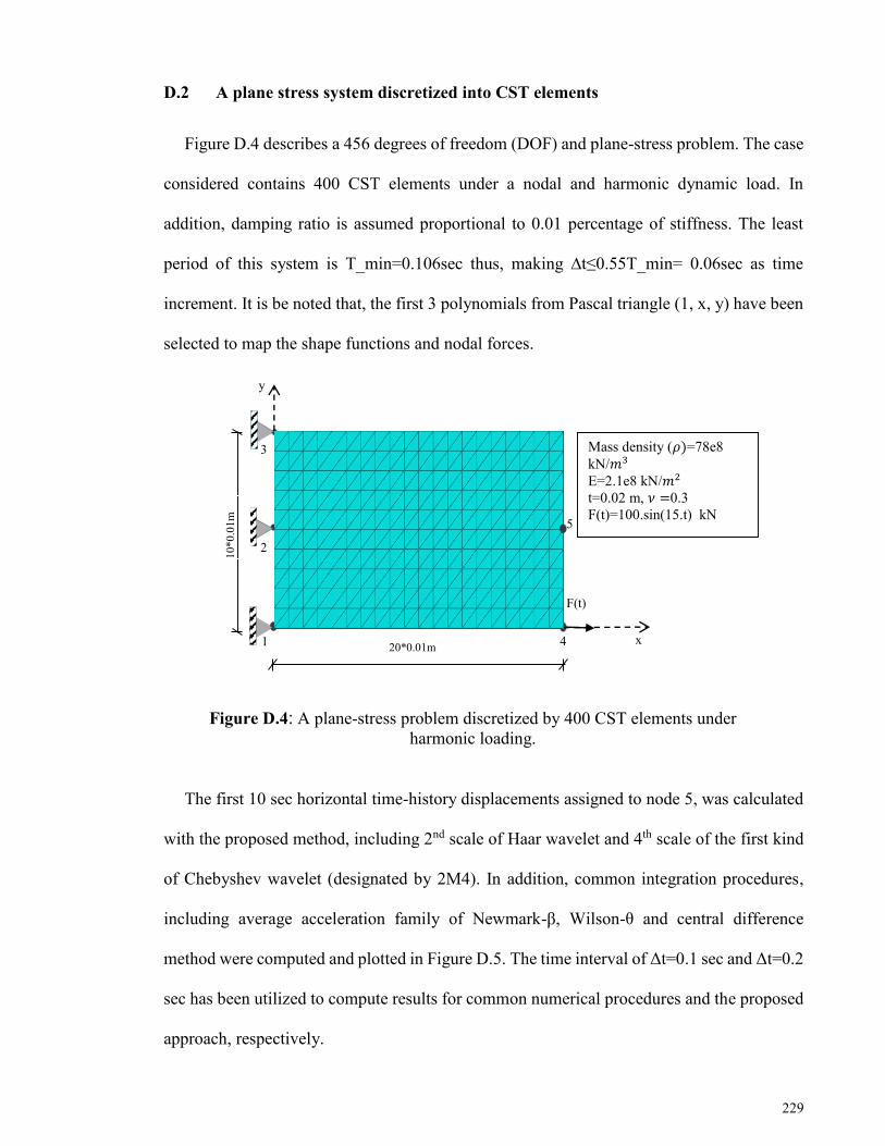
229

D.2 A plane stress system discretized into CST elements

Figure D.4 describes a 456 degrees of freedom (DOF) and plane-stress problem. The case

considered contains 400 CST elements under a nodal and harmonic dynamic load. In

addition, damping ratio is assumed proportional to 0.01 percentage of stiffness. The least

period of this system is T_min=0.106sec thus, making ∆t≤0.55T_min= 0.06sec as time

increment. It is be noted that, the first 3 polynomials from Pascal triangle (1, x, y) have been

selected to map the shape functions and nodal forces.

Figure D.4: A plane-stress problem discretized by 400 CST elements under

harmonic loading.

The first 10 sec horizontal time-history displacements assigned to node 5, was calculated

with the proposed method, including 2nd scale of Haar wavelet and 4th scale of the first kind

of Chebyshev wavelet (designated by 2M4). In addition, common integration procedures,

including average acceleration family of Newmark-β, Wilson-θ and central difference

method were computed and plotted in Figure D.5. The time interval of Δt=0.1 sec and Δt=0.2

sec has been utilized to compute results for common numerical procedures and the proposed

approach, respectively.

Mass density (𝜌)=78e8

kN/𝑚3

E=2.1e8 kN/𝑚2

t=0.02 m, 𝜈 =0.3

F(t)=100.sin(15.t) kN

5

F(t)

x

y

3

2

1

4

20*0.01m

10*0

.01

m

230

Figure D.5: Horizontal displacement of node 5, shown in Figure D.4.

As observed from Figure D.5, the results calculated using the proposed method for most

of the considered time are closer to the exact results (which was calculated by mode

supervision method). It is assumed that the 4th scale of FCW is an insufficiently accurate

scale, even though the results are precise enough. Thus, the proposed method is notable over

other numerical procedures, particularly in the real and practical cases of dynamic analysis.

It is obvious from this figure that the results calculated by central difference method is

unacceptable since conditional stability is not satisfied when Δt=0.1sec.

Figure D.6: Total average errors in horizontal displacement of node 5, shown in

Figure D.4., and relative computational time. (CH(2Mµ)= µ scale of the first

Chebyshev wavelet, CD=central difference, AAcc=average acceleration).

-1.20E-5

-7.00E-6

-2.00E-6

3.00E-6

8.00E-6

1.30E-5

0 1 2 3 4 5 6 7 8 9 10

Dis

pla

cem

ent(

m)

Time(sec)

Exact Wilson(θ=1.4)Chebyshev(2M4) Newmark(Linear Acc)Newmark(Average Acc) CD

89.31

28.6924.67

42.02

57.3849.02

0

10

20

30

40

50

60

70

80

90

100

0

20

40

60

80

100

120

140

Exact CH(2M4) Haar(2M2) CD AAcc Wilson(θ=1.4)


To

tal

Av

erag

e E

rro

rs (

%)

Tim

e Co

nsu

mp

tion

(sec)

231

Finally, total average error and computational time corresponding to the horizontal time

history displacement of node 5 is plotted in Figure D.6. It can be seen from the figure that

responses were calculated in 28.69sec by 4th scale of Chebyshev wavelet, whereas, the time

taken was 49.02sec for Wilson-θ method; although, the accuracy of results are almost the

same i.e., 16% error. Figure D.6 also highlights the efficiency of the proposed method,

particularly when the first kind of Chebyshev wavelet (known as 3D wavelet function) was

utilized.

232

Appendix E: Structural identification and damage detection results

This appendix presents some of the additional results (following by results presented in

Chapters 4 and 5 of this study) on structural identification and damage detection of different

structural systems. For this purpose, a numerical investigation is first carried out for structural

health monitoring of a simple SDOF system, numerically. Second, the proposed wavelet-

based scheme for optimum measurement of structural responses is validated for measuring

the dynamic responses of a SDOF experiment as well as a simulated 2D truss structure. Later,

some of the complementary results have been presented regarding to the incomplete

measurement of the third experiment presented in Chapter 5 (2D truss structure).

E.1 A simulated SDOF system

Figure E.1 shows an idol SDOF system with the only DOF on X direction (a shear SDOF).

The system’s characteristics are shown in the figure. This structure is subjected to two

different impact loads at the first 0-2sec of vibration analysis. The first, impact of 2 (ton)

strikes the only DOF at t=0.01sec (is shown in Figure E.1(a)) and the structure is freely

vibrated until the second impact of 4 (ton) at t=1sec (Figure E.1(b)). In addition, β is defined

as the percentage of reduction (the coefficient of damage) executed on the stiffness of the

column 2i at t=1sec. Accordingly, the time-history of acceleration known as the measured

accelerometer data (designated by Original-Acceleration) and displacement (designated by

Original-Displacement) which were calculated using Newmark method are illustrated in

Figure E.2.

233

Figure E.1: A SDOF system under impact loads at two stages of (a) 2 (ton) on

undamaged system at t=0.01sec (b) 4 (ton) on damaged system at t=1sec.

Figure E.2: The first two seconds time-history of (a) acceleration (b) displacement

of the SDOF system shown in Figure E.1.

0 0.2 0.4 0.6 0.8 1 1.2 1.4 1.6 1.8 2

-600

-400

-200

0

200

400

600

800

1000

Time(sec)

Acc

eler

atio

n(cm

/sec

2)

Original Acceleration

0 0.2 0.4 0.6 0.8 1 1.2 1.4 1.6 1.8 2

-0.1

-0.05

0

0.05

0.1

0.15

Time (sec)

Dis

plac

emen

t(cm

)

Original Displacement

𝐸 = 210𝐺𝑃𝑎 𝐼𝐶 = 25170𝑐𝑚

4 𝑙 = 400𝑐𝑚 𝐾 = 24𝐸𝐼𝐶/𝑙

3

X

𝑙 = 400𝑐𝑚

𝐼 = ∞ 𝑚 = 4 𝑡𝑜𝑛

𝐼𝑃𝐵300 𝐼𝑃𝐵300

𝐼 = ∞ 𝑚 = 4 𝑡𝑜𝑛

m

𝐼𝑃𝐵300 𝐼𝑃𝐵300

Impact 1at t=0.01sec

400𝑐𝑚

2 1i 2i 1

a b

X

Y Y

𝜷%Reducti

on

Impact 2 at t=1sec

(a)

(b)

234

In addition, the approximation of the measured acceleration is performed using different

scales of wavelet. To highlight the effect of various scales of the first kind of Chebyshev

wavelet (FCW), coefficients of this wavelet (designated by ChebyW-Coefficients), the

approximation of accelerations (designated by App-Acc-Cheby) and original accelerometer

data (designated by Orig-Acc) are depicted and compared in Figure E.3, emphasizing on the

4th and 32nd scales of FCW (designated by 2M4 and 2M32) for t=0.98-1.1sec.

Figure E.3: Coefficients of Chebyshev wavelet (FCW) for, (a) the 4th scale (b) the

32nd scale (ChebyW=Chebyshev wavelet, Acc=acceleration, App=approximation,

Orig=Original).

0.98 1 1.02 1.04 1.06 1.08 1.1

-600

-400

-200

0

200

400

600

800

1000

Time(sec)

Acc

eler

atio

n(c

m/s

ec2

)

Orig-Acc

App-Acc-Cheby

ChebyW-Coefficients(2M4)

0.98 1 1.02 1.04 1.06 1.08 1.1-800

-600

-400

-200

0

200

400

600

800

1000

Time(sec)

Acc

eler

atio

n(c

m/s

ec2

)

Orig-Acc

App-Acc-Cheby

ChebyW-Coefficients(2M32)

(a)

(b)

235

It is obviously shown in Figure E.3 that, for the purpose of an accurate decomposition in

achieving a sufficiently precise measurement, larger scales of corresponding wavelet (e.g.,

FCW, SCW or LW) shall be utilized, particularly, for the approximation of wide-frequency

content accelerometer data. Moreover, measured displacements of the SDOF system are

plotted in Figure E.4 (t=0.98-1.3sec) using d_t=0.05sec for the 2nd and 8th scales of FCW

(designated by Disp-Cheby 2M2 and 2M8) and compared with original displacements

(d_t=0.01sec) known as recorded data (due to the reduction of β=50%).

Figure E.4: The measured time-history of displacement of the SDOF system shown

in Figure E.1 at t=0.98-1.3sec (Disp-Cheby=measured displacements using

Chebyshev wavelet (FCW), Orig-Disp=original recorded displacement).

As it was anticipated, the measured displacements using the 8th scale of Chebyshev

wavelet (FCW) is closer to the originally recorded displacements rather than the 2nd scale.

Even though, in order to compare the efficiency of diverse scales of FCW in detail, the

percentile average and relative error and computation time involved of the measured

displacements at t=0-2sec, corresponding to different scales are shown in Figure E.5.

1 1.05 1.1 1.15 1.2 1.25 1.3

-0.1

-0.05

0

0.05

0.1

0.15

Time(sec)

Dis

plac

emen

t(cm

)

Disp-Cheby(2M2)

Disp-Cheby(2M8)

Orig-Disp

236

Figure E.5: Total average error and computational time for the measurement of

displacements using different scales of the first kind of Chebyshev wavelet

(Cheby=Chebyshev wavelet).

Figure E.5 demonstrates that, the complex and accurate scales of FCW (2M32 or 2M64)

achieved the considerably minimum measurement of errors, e.g., 0.0035% for the 64th scale,

however, the computation time involved surged the maximum values, e.g., 19.09sec. As a

noticeable feedback, the practice of such scales yields non-optimum computation, thus, is

incapable of online measurement. It should be noted that, because of the simple application

of SDOF and uncomplicated lateral loading, those quantities were slightly changed between

the first two scales. In other words, for the complex structures subjected to the wide-

frequency component excitation, larger scales shall be implemented.

Practically, one of the main contributions of the structural measurement is to track the

time-varying characteristics of mechanical systems, i.e., stiffness or damping of structures.

For this purpose, the time-history of stiffness for damaged and undamaged phases of

considered SDOF are plotted in Figures E.6 and E.7, respectively. For the computation of the

time-history stiffness (K), a controller coefficient was given to track displacement data bigger

than a known value (K is satisfied for u > u Controller), otherwise, the quantity of flexibility

(f=1/K) may be considered.

59.14

37.71

9.22

0.6 0.00350.66 0.83

1.06 7.57

19.09

0

5

10

15

20

25

0

10

20

30

40

50

60

70

Cheby(2M2) Cheby(2M4) Cheby(2M8) Cheby(2M32) Cheby(2M64)

Total Average Errors% Computational Time(sec)

To

tal

Av

erag

e E

rro

r (%

)

Co

mp

utatio

nal T

ime (sec)

237

Figure E.6: Stiffness (K) evaluation of the SDOF system shown in Figure E.1

(β=0%), using the measured data (shown displacements) by the 8th scale of

Chebyshev wavelet (FCW Cheby2M8).

Accordingly, in order to impose the damage scenario on the column 2i shown in Figure

E.1, β=75% is applied to reduce relevant stiffness at t=1sec. It should be noted that

d_t=0.05sec has been utilized as the time increment of the proposed measurement approach

which is appropriate for the online measurement in contrast to d_t=0.01sec for the sampling

rate of data collection. It can be seen from Figure E.7 that, the reduced stiffness and its

location on time axis is accurately monitored even by employing a large time increment.

Furthermore, the time-history of the maximum stress which is placed at the base of the

SDOF system is illustrated in Figure E.8, in order to obtain the border of elastic behavior,

and resulting in an optimum integrity and safety analysis of the considered structure.

0 0.2 0.4 0.6 0.8 1 1.2 1.4 1.6 1.8 20

0.2

0.4

0.6

0.8

1

1.2

1.4

1.6

1.8

2x 10

4

Time(sec)

Sti

ffn

ess

((N

/10

)/cm

)

Calculated K(Beta=0%)-Cheby(2M8)

2 1 0

Displacement(cm)

0 0.2 0.4 0.6 0.8 1 1.2 1.4 1.6 1.8 2

-0.1

-0.05

0

0.05

0.1

Dis

pla

cem

en

t(cm

)

238

Figure E.7: Stiffness (K) evaluation of the SDOF system shown in Figure E.1

(β=75%), using the measured data (shown displacements) by the 8th scale of


Figure E.8: Time history of maximum stress at the base of the SDOF system

shown in Figure E.1 using the measured data for (β=75%) by the 8th scale of


0 0.2 0.4 0.6 0.8 1 1.2 1.4 1.6 1.8 20

0.2

0.4

0.6

0.8

1

1.2

1.4

1.6

1.8

2x 10

4

Time(sec)

Sti

ffn

ess

((N

/10

)/cm

)

Calculated K(Beta=75%)-Cheby(2M8)

0 0.2 0.4 0.6 0.8 1 1.2 1.4 1.6 1.8 20

50

100

150

200

250

Time(sec)

Str

ess

((N

/10

)/cm

2)

Stress(max) at the Base

2 1 0

Displacement(cm)

0 0.2 0.4 0.6 0.8 1 1.2 1.4 1.6 1.8 2

-0.1

-0.05

0

0.05

0.1

Dis

pla

cem

en

t(cm

)

239

Consequently, this figure shows the effectiveness of the low scales of Chebyshev wavelet

(2M8) together with using a long time interval of numerical approximation, which is

satisfactory optimum for the online measurement of structural responses.

E.2 Optimum measurement of structural responses of a SDOF model

A simple SDOF test setup is evaluated under a regular hammer test, experimentally.

Accordingly, g= 9.81 m/sec2 is presumed as the ground acceleration. As shown in Figure

E.9, the considered system provided by two narrow aluminum columns and a rigid Plexiglas,

which are only vibrating in the x direction. In order to invoke only one DOF, the thickness

of the columns was chosen to be much narrower than its width (≅1/37). The geometry and

details of the experiment setup are shown in the figure. As illustrated in the figure, a non-

contact laser device was installed on the base in order to identify the accurate time-history of

displacements (at sampling rate 102.4).

Figure E.9: The ideal SDOF experiment setup and the schematic view, measuring

displacements by laser sensor.

Moreover, two piezoelectric sensors (accelerometers) were attached on the DOF of the

system. To evaluate the proposed method of measurement, a hammer strikes the structure

Mass= 0.279gr on SDOF

Rigid Plexiglas at SDOF

Non-contact laser sensor

to pick displacements

Thickness of columns=0.135cm

Height & wide of columns=17×5cm

The only DOF in X , K=24EI/L3

Z

Y

X

240

from 1sec after its initial condition. Accordingly, the time-history of the velocity

corresponding to the SDOF has been computed for the 4th scale of Haar and FCW (designated

by Cal-Vel-Cheby and Haar) for the time interval of d_t=0.05 sec as depicted in Figure E.10.

The results were compared against those picked by the non-contact laser sensor for

d_t=0.009766 sec (designated by Orig-Vel).

Figure E.10: Time history of velocity for SDOF system shown in Figure E.9., (a)

calculated velocity using the 4th scale of Chebyshev wavelet of the first kind (Cal-

Vel-Cheby), (b) calculated velocity using the 4th scale of Haar wavelet (Cal-Vel-

Haar).

1 1.5 2 2.5 3 3.5 4

-30

-20

-10

0

10

20

30

40

Time (sec)

Vel

oci

ty (

cm/s

2)

Cal-Vel-Cheby

Orig-vel

1 1.5 2 2.5 3 3.5 4

-40

-30

-20

-10

0

10

20

30

40

Time (sec)

Vel

ocity

(cm

/s2)

Cal-Vel-Haar

Orig-vel

(a)

(b)

241

To clarify the discrepancy between the computed results through the proposed method,

approximation of the original acceleration (accelerometer data) is plotted in Figure E.11

corresponding to the 4th scale of Haar and Chebyshev wavelet (FCW) by illustrating the

wavelet coefficients for 1 to 1.2 sec.

Figure E.11: Coefficients of wavelet for the 4th scale of (a) ChebyW-

Coefficients=Chebyshev wavelet (FCW), (b) HaarW-Coefficients=Haar wavelet

(App-Acc= approximation of original acceleration).

1 1.02 1.04 1.06 1.08 1.1 1.12 1.14 1.16 1.18 1.2

-4000

-3000

-2000

-1000

0

1000

2000

3000

Time(sec)

Acc

eler

atio

n-(c

m/s

ec2)

Orig-Acc

App-Acc-Cheby

ChebyW-Coefficients

1 1.02 1.04 1.06 1.08 1.1 1.12 1.14 1.16 1.18 1.2

-4000

-3000

-2000

-1000

0

1000

2000

3000

4000

Time(sec)

Acc

eler

atio

n-(

cm/s

ec2

)

Orig-Acc

App-Acc-Haar

HaarW-Coefficients

(a)

(b)

242

Figures E.10 and E.11 clearly demonstrate the source of significant errors of Haar wavelet

(2M=4) for d_t=0.05 sec, while it is shown that details of the acceleration are accurately

captured by the coefficients of FCW for the same conditions. Therefore, a sufficiently precise

approximation is satisfied at the first step of the proposed scheme. Furthermore, to evaluate

the practice of various scale of Haar wavelet in detail, computed responses for the same

d_t=0.05 sec and 8th, 32nd and 64th scales of simple Haar wavelet (designated by HA(2M))

were compared with the 4th scale of complex Chebyshev wavelet (FCW). The results depicted

in Figure E.12 are from the computational time involved and percentile total average error

(PTAE) point of view.

Figure E.12: Computational time and PTAE for various scale of Haar (HA) and the

4th scale of the first kind of Chebyshev wavelet (Cheby).

It is apparant from Figure E.12 that for the accurate scales of 2D and simple Haar wavelet

(2M64), the cost of analysis is dramatically increased. However, the optimum results can be

computed even using a low scale of 3D and complex Chebyshev wavelet (FCW).

Consequently, it is shown that the practice of Haar wavelet is not applicable for the online

measurement of dynamic responses, however, for an initial evaluation it may be considered

where the fastest computation is satisfied by implementation of this basis function.

Eventually, the time-history of displacement of the only DOF is optimally calculated through

the proposed measurement scheme, particularly, using a long time interval of d_t=0.05 sec

by the 4th scale of FCW (designated by Cal-Disp-Cheby) and is compared with those

1.02

261

935.3

0.630.42

8.6117.53

0

5

10

15

20

0

50

100

150

200

250

300

Cheby(2M4) HA(2M8) HA(2M32) HA(2M64)


243

measured by the laser sensor (Orig-Disp) at the sampling rate of 102.4 S/s (shown in Figure

E.13).

Figure E.13: The first 6 sec time-history displacement of SDOF system shown in

Figure E.9 (Cal-Disp-Cheby = Calculated displacement using Chebyshev wavelet

FCW, Orig-Disp=Original displacement).

The capability of the proposed algorithm for measurement is clearly illustrated in Figure

E.13, using low scales of Chebyshev wavelet. It should be pointed out again that details of

the broad-frequency component acceleration are completely captured by the diverse scale of

this comprehensive wavelet function in contrast to the simple Haar wavelet. Finally, the third

derivative of displacement with respect to time namely, Jerk (�⃛�(t)) is considered using the 8th

scale of FCW (designated by computed jerk), as depicted in Figure E.14 and compared with

a normal incremental calculation (d(Acc)/dt) for the long interval of d_t=0.5 sec. Moreover,

it was shown before that the measurement of this value is very helpful to make an engineering

judgment on the behavior of a dynamic system.

Figure E.14 shows that the proposed method optimally and exactly detects the time of the

strike at the first second in contrast with the normal incremental calculation. Overall, it is

demonstrated that the quantity of jerk as one of the reliable criteria of dynamic behavior is

0 1 2 3 4 5 6

-0.4

-0.3

-0.2

-0.1

0

0.1

0.2

0.3

0.4

Time (sec)

Dis

plac

emen

t (cm

)

Cal-Disp-Cheby

Orig-Disp

244

optimally measured through the proposed method which is capable of optimal and online

measurement of dynamic responses.

Figure E.14: The first 7 sec analysis of the third derivative of displacement (jerk).

(a) 0-7 sec computed jerk using the 8th scale of Chenyshev wavelet (FCW) vs.

normal calculation of the derivative with respect to time (d(Acc)/dt). (b) Zooming

plane on 0.9-1.3 sec.

E.3 A 2D truss constructed with bar elements coupled with damage

Figure E.15 describes a pin-jointed and 2D truss composed of nine DOFs and 10 members.

This structure is excited for 6sec by a harmonic loading (F(t)=20.Sin(15t)_N) which is

applied on node 3, shown in Figure E.15. Additionally, the characteristics of all members are

0 1 2 3 4 5 6 7-4

-3

-2

-1

0

1

2

3

4x 10

6

Time(sec)

Jerk

(cm

/sec

3)

Computed Jerk (2M=8, dn=0.5)

d(Acc)/dt (dn=0.5)

0.95 1 1.05 1.1 1.15 1.2 1.25 1.3-1

-0.8

-0.6

-0.4

-0.2

0

0.2

0.4

0.6

0.8

1

x 106

Time(sec)

Jerk

(cm

/sec

3)

× 10−6

× 10−5

(a)

(b)

245

constant and addressed in the figure, as well as mass per length, modulus of elasticity, the

cross-sectional area and the geometric information. To evaluate a damaged scenario (in

overall linear behavior), it is assumed that at the 3rd second of excitation, because of a local

exclusive motivation such as a strong explosion, only two internal members of 1 and 2

(shown in Figure E.15(a)) are completely collapsed. The current configuration is shown in

Figure E.15(b), corresponding to t=3-6sec of loading. Equivalently, accelerometer data

associated on each DOF is recorded using Newmark scheme at the sampling rate of 100 or

d_t=0.01sec (a schematic view is illustrated in the figure on node 2).

Figure E.15: A 2D and pin-jointed truss under a harmonic loading at 6 sec (a)

reference configuration; intact system, (b) updated configuration; elements 1 and 2

are removed at t=3 sec.

In addition, the first 6sec time-history of acceleration known as measured accelerometer

data corresponding to the vertical and horizontal DOF of node 3 (shown in Figure E.15) is

plotted in Figure E.16. Therefore, for the further operations on node 3, such as the

3 5 4

1 2 3

4 5 6

1 2 3

4 5 6

1 2

2×2 m

2 m

E=70 GPa, �̅� = 50 kg/m, A= 1e-4 m2, F(t)=20. Sin(15t)_N

Numbering of DOFs :

Node number 1 2 3 4 5 6

Horizontal DOF - 1 3 - 6 8

Vertical DOF - 2 4 5 7 9

F(t)

F(t)

246

measurement of either integration or derivatives of responses in time domain,

aforementioned data is used.

Figure E.16: The first 6 sec time-history of the acquired accelerometer data for (a)

DOF=3, (b) DOF=4.

The displacement measurement is accomplished for any DOF, once the corresponding

accelerometer data is considered. For example, the time-history of displacement for the

horizontal DOF of node 2 (DOF=1) was measured from t=2.9-6sec using the 4th and the 8th

scales of Chebyshev wavelet (FCW) and depicted in Figure E.17. It is observed that,

0 1 2 3 4 5 6-0.25

-0.2

-0.15

-0.1

-0.05

0

0.05

0.1

0.15

0.2

0.25Acceleration DOF-3

Time(sec)

Acc

eler

atio

n(m

/sec

2)

0 1 2 3 4 5 6-0.2

-0.15

-0.1

-0.05

0

0.05

0.1

0.15Acceleration DOF-4

Time(sec)

Acc

eler

atio

n(m

/sec

2)

(a)

(b)

247

considerably large computational time increment of d_t=0.1sec (designated by ∆𝑡𝑤) was

utilized while, it was d_t=0.01sec (designated by ∆𝑡𝑠or sampling rate of 100 S/s) for recording

original data.

Figure E. 17: The measured displacements (Disp) of DOF=1 for t=2.9-6 sec using

(a) the 8th scale of Chebyshev wavelet, FCW (Cheby2M8), (b) the 4th scale of

Chebyshev wavelet, FCW (Cheby2M4), (∆𝒕𝒘= d_t wavelet and ∆𝒕

𝒔= d_t original

sampling rate).

It can be induced from Figure E.17 that, despite the implementation of a very large time

increment, the accuracy of the measured displacement is sufficient, particularly, at the start

of the damage scenario (at t=3sec). The reason for this lies on the capability of the wavelet

3 3.5 4 4.5 5 5.5 6-3

-2

-1

0

1

2

x 10-5

Time (sec)

Dis

plac

emen

t(m

)

Disp-Cheby(2M8)

Orig-Disp

3 3.5 4 4.5 5 5.5 6-3

-2

-1

0

1

2

x 10-5

Time (sec)

Dis

plac

emen

t(m

)

Disp-Cheby(2M4)

Orig-Disp

(a)

(b)

DOF=1, ∆𝑡𝑤=0.1sec

∆𝑡𝑠=0.01sec

DOF=1, ∆𝑡𝑤=0.1sec

∆𝑡𝑠=0.01sec

248

in which that, highly transient structural responses are precisely captured in the vicinity of

sudden changes of the inherent characteristics. As was mentioned earlier, to achieve a more

accurate measurement, larger scales of wavelet shall be utilized. However, from the

optimization point of view it may be unnecessary for simple structures under harmonic

loadings. Subsequently, the time-history of jerk for the horizontal DOF of node 5 (DOF=6)

was measured from t=2.9-3.5sec using the 8th scale of FCW and compared to the normal

incremental calculation of jerk for time instance of d_t=0.01sec shown in Figure E.18. This

figure shows that, because of the considered short computational time interval, the normal

incremental results are still reliable.

Figure E.18: The measured time-history of jerk for DOF=6 and t=2.9-3.5sec, using

the 8th scale of Chebyshev wavelet, FCW (Cheby2M8) and normal incremental

derivative for ∆t=0.01sec.

For the aim of damage localization, the jerk measurement is reasonably valuable, while,

this quantity shows one of the very sensitive dynamic response to the changes of the physical

parameters or geometry of structures. Finally, the efficiency of the proposed method for the

purpose of an online measurement is demonstrated in Figure E.19. The time-history of jerk

is illustrated for t=0-6sec using a very large time interval of d_t=0.5sec (DOF 7 represents

3 3.1 3.2 3.3 3.4 3.5

-40

-30

-20

-10

0

10

20

30

Time(sec)

Jerk

(cm

/sec

3)

Jerk-Cheby(2M8)

Incremental Jerk

DOF=6, ∆𝑡=0.01sec

249

the vertical DOF of node 5). It is clearly distinguishable from the figure that the normal

incremental computation of jerk is disable to measure this quantity at d_t=0.5sec. In contrast,

the exact location of damage on time domain is optimally detected by measuring the value

of jerk using the proposed method. It is clearly observed in Figure E.19(b), there is a

significant fluctuation on the measured quantity of jerk at undamaged stage. This is most

likely due to the same direction of the externally applied force with corresponding DOF.

Figure E.19: The measured time-history of jerk for t=0-6 sec, using the 8th scale of

Chebyshev wavelet, FCW (Cheby2M8) and normal incremental derivative for

∆t=0.5 sec (a) DOF=1, (b) DOF=7.

0 1 2 3 4 5 6-30

-20

-10

0

10

20

30

Time(sec)

Jerk

(cm

/sec

3)

Jerk-Cheby(2M8)

Incremental Jerk

0 1 2 3 4 5 6-15

-10

-5

0

5

10

15

Time(sec)

Jerk

(cm

/sec

3)

Jerk-Cheby(2M8)

Incremental Jerk

(a)

(b)



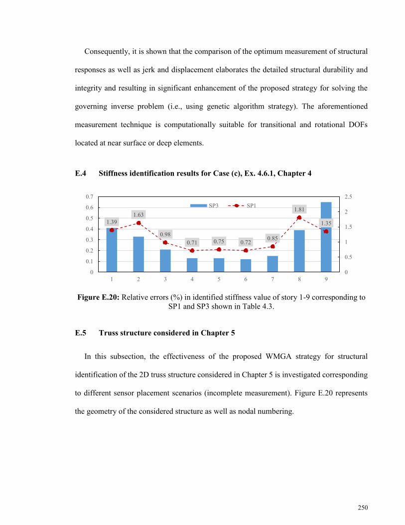
250

Consequently, it is shown that the comparison of the optimum measurement of structural

responses as well as jerk and displacement elaborates the detailed structural durability and

integrity and resulting in significant enhancement of the proposed strategy for solving the

governing inverse problem (i.e., using genetic algorithm strategy). The aforementioned

measurement technique is computationally suitable for transitional and rotational DOFs

located at near surface or deep elements.

E.4 Stiffness identification results for Case (c), Ex. 4.6.1, Chapter 4

Figure E.20: Relative errors (%) in identified stiffness value of story 1-9 corresponding to

SP1 and SP3 shown in Table 4.3.

E.5 Truss structure considered in Chapter 5

In this subsection, the effectiveness of the proposed WMGA strategy for structural

identification of the 2D truss structure considered in Chapter 5 is investigated corresponding

to different sensor placement scenarios (incomplete measurement). Figure E.20 represents

the geometry of the considered structure as well as nodal numbering.

1.39

1.63

0.98

0.71 0.75 0.720.85

1.81

1.35

0

0.5

1

1.5

2

2.5

0

0.1

0.2

0.3

0.4

0.5

0.6

0.7

1 2 3 4 5 6 7 8 9

SP3 SP1

251

Figure E.21: The schematic view of the test setup used for 2D truss; the main layout of

the test, elements and nodes numbering, (a) intact structure, (b) damage is imposed on

elements 4 and 12.

In referring to Chapter 5, there are three loadings are governed on this structure at 8-x, 5-

y and 4-y. The identification of intact structure shown in Figure E.21(a) is considered due to

the incomplete measurement of responses. For this purpose, the program for optimum sensor

placement is run for the total number of sensors available and representing the sensor

placement scenarios (SP) and results are shown in Table E.1.

Table E.1: Optimum sensor placements.

Total number of

available

sensors (SP)

Preferred measured DOFs

3 3-y, 4-y, 7-x

6 3-x, 4-x, 4-y, 5-x, 5-y, 7-x

9 3-x, 3-y, 4-x, 4-y, 5-x, 5-y, 7-x, 7-y, 8-x

12 2-y, 3-x, 3-y, 4-x, 4-y, 5-x, 5-y, 7-x, 7-y, 8-x, 6-x, 6-y

Accordingly, the structural identification of intact structure is conducted using WMGA

strategy corresponding to different sensor placements displayed in Table E.1 and the

maximum error (%) obtained for identified stiffness of each structural element is depicted in

Figure E.22.

(a)

(b)

252

It was anticipated that, the accurate identification is achieved by the most complete

measurement as SP12 shown in Figure E.22. This figure obviously shows that, for elements

between two measured DOFs the most reliable identifications are obtained. In contrast, for

elements that the adjacent DOFs are not measured the maximum error reached to the highest

value. It should be noted here that, the algorithm of optimum sensor placement compares the

closeness of results obtained for reduced system and simulated response of the whole

structure. For this reason, the highest influence of element’s stiffness is seen on its coupled

DOFs, and therefore for elements that at least one adjacent DOFs is measured the identified

stiffness is much more accurate.

Figure E.22: The maximum error (%) obtained for identified stiffness of each

structural element shown in Figure E.20, (a) SP3, (b) SP6, (c) SP9, (d) SP12.

0

50

100

1 2 3 4 5 6 7 8 9 10 11 12 13

Maximum error in identified stiffness (%)

0

50

100

1 2 3 4 5 6 7 8 9 10 11 12 13

0

20

40

1 2 3 4 5 6 7 8 9 10 11 12 13

0

10

20

1 2 3 4 5 6 7 8 9 10 11 12 13

(a)

(b)

(c)

(d)

Element Number

253

REFERENCES

Aktan, A.E., Lee, K.L., Chuntavan, C., and Aksel, T. (1994). Modal testing for structural

identification and condition assessment of constructed facilities. Paper presented at

the Proceedings-Spie the International Society for Optical Engineering.

Akula, V.R., and Ganguli, R. (2003). Finite element model updating for helicopter rotor blade

using genetic algorithm. AIAA Journal, 41(3): 554-556.

Babolian, E., and Fattahzadeh, F. (2007). Numerical solution of differential equations by

using Chebyshev wavelet operational matrix of integration. Applied Mathematics and

Computation, 188(1): 417-426.

Balamurugan, R., Ramakrishnan, C.V., and Singh, N. (2008). Performance evaluation of a

two stage adaptive genetic algorithm (TSAGA) in structural topology optimization.

Applied Soft Computing, 8(4): 1607-1624.

Bathe, K.J. (2006). Finite element procedures: Klaus-Jurgen Bathe.

Bathe, K.J., and Ramaswamy, S. (1980). An accelerated subspace iteration method.

Computer Methods in Applied Mechanics and Engineering, 23(3): 313-331.

Bathe, K.J., and Wilson, E.L. (1972a). Large eigenvalue problems in dynamic analysis.

Journal of the Engineering Mechanics Division, 98(6): 1471-1485.

Bathe, K.J., and Wilson, E.L. (1972b). Stability and accuracy analysis of direct integration

methods. Earthquake Engineering & Structural Dynamics, 1(3): 283-291.

Bathe, K.J., and Wilson, E.L. (1973). Stability and accuracy analysis of direct integration

methods. Earthquake Engineering and Structural Dynamics, 1(3): 283-291.

Beck, J.L., and Katafygiotis, L.S. (1998). Updating models and their uncertainties. I:

Bayesian statistical framework. Journal of Engineering Mechanics, 124(4): 455-461.

Bicanic, N., and Chen, H.P. (1998). Damage identification in framed structures using natural

frequencies. International Journal for Numerical Methods in Engineering(40): 4451-

4468.

Bracewell, R. (1965). The Fourier transform and its applications. New York.

Brigham, E.O. (1988). The fast Fourier transform and its applications (Vol. 1): Prentice Hall

Englewood Cliffs, NJ.

254

Buades, A., Coll, B., and Morel, J.M. (2005). A review of image denoising algorithms, with

a new one. Multiscale Modeling & Simulation, 4(2): 490-530.

Caravani, P., Watson, M.L., and Thomson, W.T. (1977). Recursive least-squares time

domain identification of structural parameters. Journal of Applied Mechanics, 44(1):

135-140.

Cattani, C. (2004). Haar wavelet-based technique for sharp jumps classification.

Mathematical and Computer Modelling, 39(2): 255-278.

Cawley, P., and Adams, R.D. (1979). The location of defects in structures from

measurements of natural frequencies. The Journal of Strain Analysis for Engineering

Design, 14(2): 49-57.

Chang, S.Y. (2002). Explicit pseudodynamic algorithm with unconditional stability. Journal

of Engineering Mechanics, 128(9): 935-947.

Chang, S.Y. (2010). A new family of explicit methods for linear structural dynamics.

Computers & Structures, 88(11): 755-772.

Chen, C.F., and Hsiao, C.H. (1997). Haar wavelet method for solving lumped and

distributed-parameter systems. Paper presented at the Control Theory and

Applications, IEE Proceedings.

Chui, C.K. (1992). Wavelet analysis and its applications, vol. 1, An introduction to wavelets:

Academic Press.

Chui, C.K. (1995). Wavelet analysis and its applications. Texas A&M University College

Station Department of Mathematics: DTIC Document.

Chui, C.K. (2014). An introduction to wavelets (Vol. 1): Academic press.

Chung, J., and Lee, J.M. (1994). A new family of explicit time integration methods for linear

and non‐linear structural dynamics. International Journal for Numerical Methods in

Engineering, 37(23): 3961-3976.

Cohen, A., Dahmen, W., and DeVore, R. (2003). Adaptive wavelet schemes for nonlinear

variational problems. SIAM Journal on Numerical Analysis, 41(5): 1785-1823.

Cohen, L. (1989). Time-frequency distributions-a review. Proceedings of the IEEE, 77(7):

941-981.

Cooley, J.W., and Tukey, J.W. (1965). An algorithm for the machine calculation of complex

Fourier series. Mathematics of Computation, 19(90): 297-301.

255

Creed, S. (1987). Assessment of large engineering structures using data collected during in-

service loading. Procedings of Structural Assessment Based on Full and Large Scale

Testing.

Dahmen, W., Kurdila, A., and Oswald, P. (1997). Multiscale wavelet methods for partial

differential equations (Vol. 6): Academic Press.

Daubechies, I. (1988). Orthonormal bases of compactly supported wavelets.

Communications on Pure and Applied Mathematics, 41(7): 909-996.

Daubechies, I. (1992). Ten lectures on wavelets (Vol. 61): SIAM.

Deb, K., and Agrawal, R.B. (1994). Simulated binary crossover for continuous search space.

Complex Systems, 9(3): 1-15.

Deb, K., and Gulati, S. (2001). Design of truss-structures for minimum weight using genetic

algorithms. Finite Elements in Analysis and Design, 37(5): 447-465.

Debnath, L., and Bhatta, D. (2014). Integral transforms and their applications: CRC press.

Devore, R.A., Jawerth, B., and Lucier, B.J. (1992). Image compression through wavelet

transform coding. Information Theory, IEEE Transactions on, 38(2): 719-746.

Dipasquale, E., and Cakmak, A.S. (1990). Seismic damage assessment using linear models.

Soil Dynamics and Earthquake Engineering, 9(4): 194-215.

Dokainish, M.A., and Subbaraj, K. (1989). A survey of direct time-integration methods in

computational structural dynamics—I. Explicit methods. Computers & Structures,

32(6): 1371-1386.

Ewins. (2000). Modal testing: theory, practice and application (Vol. 2): Research studies

press Baldock.

Fan, W., and Qiao, P. (2009). A 2-D continuous wavelet transform of mode shape data for

damage detection of plate structures. International Journal of Solids and Structures,

46(25): 4379-4395.

Fang, S.E., and Perera, R. (2009). Power mode shapes for early damage detection in linear

structures. Journal of Sound and Vibration, 324(1): 40-56.

Farge, M. (1992). Wavelet transforms and their applications to turbulence. Annual Review of

Fluid Mechanics, 24(1): 395-458.

256

Farrar, C.R., Baker, W.E., Bell, T.M., Cone, K.M., Darling, T.W., Duffey, T.A., . . . Migliori,

A. (1994). Dynamic characterization and damage detection in the I-40 bridge over

the Rio Grande. Los Alamos National Lab., NM (United States).

Faverjon, B., and Sinou, J.J. (2009). Identification of an open crack in a beam using an a

posteriori error estimator of the frequency response functions with noisy

measurements. European Journal of Mechanics and Solids, 28(1): 75-85.

Franulović, M., Basan, R., and Prebil, I. (2009). Genetic algorithm in material model

parameters’ identification for low-cycle fatigue. Computational Materials Science,

45(2): 505-510.

Friswell, M., and Mottershead, J.E. (1995). Finite element model updating in structural

dynamics (Vol. 38): Springer Science & Business Media.

Furuta, H., Kameda, T., Nakahara, K., Takahashi, Y., and Frangopol, D.M. (2006). Optimal

bridge maintenance planning using improved multi-objective genetic algorithm.

Structure and Infrastructure Engineering, 2(1): 33-41.

Gabor, D. (1946). Theory of communication. Part 1: The analysis of information. Journal of

the Institution of Electrical Engineers-Part III: Radio and Communication

Engineering, 93(26): 429-441.

Galli, A.W., Heydt, G.T., and Ribeiro, P.F. (1996). Exploring the power of wavelet analysis.

Computer Applications in Power, IEEE, 9(4): 37-41.

Ghanem, R., and Shinozuka, M. (1995). Structural-system identification. I: Theory. Journal

of Engineering Mechanics, 121(2): 255-264.

Goedecker, S., and Ivanov, O. (1998). The solution of multi-scale partial differential

equations using wavelets. ARXiv Preprint Physics/9803011. doi: 10.1063/1.168739

Goldberg, D.E., and Holland, J.H. (1988). Genetic algorithms and machine learning.

Machine Learning, 3(2): 95-99.

Grossman, A., Morlet, J., and Paul, T. (1986). Transforms associated to square integrable

group representations. ii: Examples. Paper presented at the Annales de l'IHP

Physique Théorique.

Grossmann, A., and Morlet, J. (1984). Decomposition of Hardy functions into square

integrable wavelets of constant shape. SIAM Journal on Mathematical Analysis,

15(4): 723-736.

257

Grossmann, A., Morlet, J., and Paul, T. (1985). Transforms associated to square integrable

group representations. I. General results. Journal of Mathematical Physics, 26(10):

2473-2479.

Gurley, K., and Kareem, A. (1999). Applications of wavelet transforms in earthquake, wind

and ocean engineering. Engineering Structures, 21(2): 149-167.

Haar, A. (1910). Zur theorie der orthogonalen funktionensysteme. Mathematische Annalen,

69(3): 331-371.

Haberman, R. (2013). Applied partial differential equations with Fourier series and boundary

value problems. Applied Mathematics and Computation, 10: 12.

Heil, C.E., and Walnut, D.F. (1989). Continuous and discrete wavelet transforms. SIAM

Review, 31(4): 628-666.

Hemez, F.M., and Doebling, S.W. (1999). A validation of Bayesian finite element model

updating for linear dynamics. Paper presented at the 17th SEM International Modal

Analysis Conference.

Hubbard, B.B. (1998). The world according to wavelets the story of a mathematical

technique in the making: Universities Press.

Hughes, T.J.R. (2012). The finite element method: linear static and dynamic finite element

analysis: Courier Corporation.

Imregun, M., Visser, W.J., and Ewins, D.J. (1995). Finite element model updating using

frequency response function data: I. Theory and initial investigation. Mechanical

Systems and Signal Processing, 9(2): 187-202.

Jaffard, S., Meyer, Y., and Ryan, R.D. (2001). Wavelets: tools for science and technology:

SIAM.

Jeffrey, A. (2001). Advanced engineering mathematics: Academic Press.

Jinwen, T.D.Q.W.W. (2009). The finite element model updating of structure based on

wavelet packet analysis and support vector machines. Journal of Huazhong

University of Science and Technology (Nature Science Edition), 6: 027.

Jung, D.S., and Kim, C.Y. (2009). FE model updating based on hybrid genetic algorithm and

its verification on numerical bridge model. Structural Engineering and Mechanics,

32(5): 667-683.

258

Kalman, R.E. (1960). A new approach to linear filtering and prediction problems. Journal of

Fluids Engineering, 82(1): 35-45.

Kim, H.M., and Bartkowicz, T.J. (1993). Damage detection and health monitoring of large

space structures. Sound and Vibration, 27: 12-12.

Kitagawa, G. (1996). Monte Carlo filter and smoother for non-Gaussian nonlinear state space

models. Journal of Computational and Graphical Statistics, 5(1): 1-25.

Ko, J.M., and Ni, Y.Q. (2005). Technology developments in structural health monitoring of

large-scale bridges. Engineering Structures, 27(12): 1715-1725.

Ko, J.M., Ni, Y.Q., and Chan, H.T. (1999). Dynamic monitoring of structural health in cable-

supported bridges. Paper presented at the 1999 Symposium on Smart Structures and

Materials.

Koh, C.G., Hong, B., and Liaw, C.Y. (2003). Substructural and progressive structural

identification methods. Engineering Structures, 25(12): 1551-1563.

Körner, Thomas William. (1989). Fourier analysis: Cambridge university press.

Kougioumtzoglou, I.A., and Spanos, P.D. (2013). An identification approach for linear and

nonlinear time-variant structural systems via harmonic wavelets. Mechanical Systems

and Signal Processing, 37(1): 338-352.

Kwak, H.G., and Kim, J. (2009). An integrated genetic algorithm complemented with direct

search for optimum design of RC frames. Computer-Aided Design, 41(7): 490-500.

Lepik, U. (2005). Numerical solution of differential equations using Haar wavelets.

Mathematics and Computers in Simulation, 68(2): 127-143.

Lepik, U. (2008a). Haar wavelet method for solving higher order differential equations.

International Journal of Mathematics & Computation, 1(N08): 84-94.

Lepik, U. (2008b). Haar wavelet method for solving higher order differential equations.

International Journal of Mathematics & Computation™, 1(N08): 84-94.

Lepik, U. (2008c). Solving integral and differential equations by the aid of non-uniform Haar

wavelets. Applied Mathematics and Computation, 198(1): 326-332.

Lepik, U. (2009a). Haar wavelet method for solving stiff differential equations. Mathematical

Modelling and Analysis, 14(4): 467-481.

259

Lepik, U. (2009b). Solving fractional integral equations by the Haar wavelet method. Applied

Mathematics and Computation, 214(2): 468-478.

Lévy, P. (1954). Le mouvement brownien. Mémorial des Sciences Mathématiques, 126: 1-

84.

Lindholm, B.E., and West, R.L. (1996). A Bayesian statistics approach to updating finite

element models with frequency response data (part i: theory). Paper presented at the

Proceedings of the 14th International Modal Analysis Conference.

Ling, S.H., and Leung, F.H.F. (2007). An improved genetic algorithm with average-bound

crossover and wavelet mutation operations. Soft Computing, 11(1): 7-31.

Ling, X., and Haldar, A. (2004). Element level system identification with unknown input

with Rayleigh damping. Journal of Engineering Mechanics, 130(8): 877-885.

Littlewood, J.E., and Paley, R.E.A. (1931). Theorems on Fourier series and power series.

Journal of the London Mathematical Society, 1(3): 230-233.

Liu, G.R., and Chen, S.C. (2002). A novel technique for inverse identification of distributed

stiffness factor in structures. Journal of Sound and Vibration, 254(5): 823-835.

Liu, M., Frangopol, D.M., and Kim, S. (2009). Bridge system performance assessment from

structural health monitoring: a case study. Journal of Structural Engineering, 135(6):

733-742.

Liu, X., Lieven, N.A.J., and Escamilla, A.P.J. (2009). Frequency response function shape-

based methods for structural damage localisation. Mechanical Systems and Signal

Processing, 23(4): 1243-1259.

Ljung, L., and Glover, K. (1981). Frequency domain versus time domain methods in system

identification. Automatica, 17(1): 71-86.

Mackenzie, D. (2001). Wavelets: seeing the forest and the trees. Beyond Discovery (National

Academy of Sciences, Washington, 2001).

Mahdavi, S.H., and Razak, H.A. (2013). A wavelet-based approach for vibration analysis of

framed structures. Applied Mathematics and Computation, 220: 414-428.

Mahdavi, S.H., and Razak, H.A. (2015a). A comparative study on optimal structural

dynamics using wavelet functions. Mathematical Problems in Engineering.

260

Mahdavi, S.H., and Razak, H.A. (2015b). An efficient iterative scheme for solution of non-

linear problems using family of Chebyshev operations. Mathematical Problems in

Engineering.

Mahdavi, S.H., and Razak, H.A. (2015c). Indirect time integration scheme for dynamic

analysis of space structures using wavelet functions. Journal of Engineering

Mechanics (ASCE).

Mahdavi, S.H., and Shojaee, S. (2013). Optimum time history analysis of SDOF structures

using free scale of Haar wavelet. Structural Engineering and Mechanics, 45(1): 95-

110.

Maia, N.M.M., and Esilva, J.M.M. (1997). Theoretical and experimental modal analysis:

Research Studies Press Taunton.

Maleknejad, K., Sohrabi, S., and Rostami, Y. (2007). Numerical solution of nonlinear

Volterra integral equations of the second kind by using Chebyshev polynomials.

Applied Mathematics and Computation, 188(1): 123-128.

Mallat, S. (1999). A wavelet tour of signal processing, (wavelet analysis & its applications).

Mallat, S.G. (1989a). Multiresolution approximations and wavelet orthonormal bases.

Transactions of the American Mathematical Society, 315(1): 69-87.

Mallat, S.G. (1989b). A theory for multiresolution signal decomposition: the wavelet

representation. Pattern Analysis and Machine Intelligence, IEEE Transactions,

11(7): 674-693.

Mallat, S.G. (1999). A wavelet tour of signal processing: Academic Press.

Marano, G.C., Quaranta, G., and Monti, G. (2011). Modified genetic algorithm for the

dynamic identification of structural systems using incomplete measurements.

Computer‐Aided Civil and Infrastructure Engineering, 26(2): 92-110.

Mares, C., Mottershead, J.E., and Friswell, M.I. (2006). Stochastic model updating: part 1—

theory and simulated example. Mechanical Systems and Signal Processing, 20(7):

1674-1695.

Marwala, T. (2002). Finite element model updating using wavelet data and genetic algorithm.

Journal of Aircraft, 39(4): 709-711.

Marwala, T., and Sibisi, S. (2005). Finite element model updating using Bayesian framework

and modal properties. Journal of Aircraft, 42(1): 275-278.

261

Mason, J.C., and Handscomb, D.C. (2002). Chebyshev polynomials: CRC Press.

Maybeck, P.S. (1982). Stochastic models, estimation, and control (Vol. 3): Academic Press.

Messina, A., Williams, E.J., and Contursi, T. (1998). Structural damage detection by a

sensitivity and statistical-based method. Journal of Sound and Vibration, 216(5): 791-

808.

Meyer, Y. (1989). Orthonormal wavelets Wavelets (pp. 21-37): Springer.

Meyer, Y. (1993). Wavelets-algorithms and applications. Society for Industrial and Applied

Mathematics Translation, 1: 1-142.

Michalewicz, Z. (1996). Genetic algorithms+ data structures= evolution programs: Springer

Science & Business Media.

Michalewicz, Z. (2013). Genetic algorithms+ data structures= evolution programs: Springer

Science & Business Media.

Migliori, A. (1991). Resonant ultrasound spectroscopy: Google Patents.

Newland, D.E. (1993). Harmonic wavelet analysis. Proceedings of the Royal Society of

London. Series A: Mathematical and Physical Sciences, 443(1917): 203-225.

Ni, Y.Q., Zhou, X.T., and Ko, J.M. (2006). Experimental investigation of seismic damage

identification using PCA-compressed frequency response functions and neural

networks. Journal of Sound and Vibration, 290(1): 242-263.

Nooshin, H., and Disney, P. (1991). Elements of formian. Computers & Structures, 41(6):

1183-1215.

Okasha, N.M., and Frangopol, D.M. (2009). Lifetime-oriented multi-objective optimization

of structural maintenance considering system reliability, redundancy and life-cycle

cost using GA. Structural Safety, 31(6): 460-474.

Oppenheim, A.V., Schafer, R.W., and Buck, J.R. (1989). Discrete-time signal processing

(Vol. 2): Prentice-Hall Englewood Cliffs.

Perera, R., and Ruiz, A. (2008). A multistage FE updating procedure for damage

identification in large-scale structures based on multiobjective evolutionary

optimization. Mechanical Systems and Signal Processing, 22(4): 970-991.

262

Perry, M.J. (2007). Modified genetic algorithm approach to system identification with

structural and offshore application. National University of Singapore.

Perry, M.J., Koh, C.G., and Choo, Y.S. (2006). Modified genetic algorithm strategy for

structural identification. Computers & Structures, 84(8): 529-540.

Qiao, P., and Cao, M. (2008). Waveform fractal dimension for mode shape-based damage

identification of beam-type structures. International Journal of Solids and Structures,

45(22): 5946-5961.

Qiao, P., Lu, K., Lestari, W., and Wang, J. (2007). Curvature mode shape-based damage

detection in composite laminated plates. Composite Structures, 80(3): 409-428.

Quek, S.T., Wang, Q., Zhang, L., and Ang, K.K. (2001). Sensitivity analysis of crack

detection in beams by wavelet technique. International Journal of Mechanical

Sciences, 43(12): 2899-2910.

Rader, C.M. (1968). Discrete Fourier transforms when the number of data samples is prime.

Proceedings of the IEEE, 56(6): 1107-1108.

Razzaghi, M., and Yousefi, S. (2000). Legendre wavelets direct method for variational

problems. Mathematics and Computers in Simulation, 53(3): 185-192.

Razzaghi, M., and Yousefi, S. (2001). Legendre wavelets method for the solution of

nonlinear problems in the calculus of variations. Mathematical and Computer

Modelling, 34(1): 45-54.

Ren, W.X., and Sun, Z.S. (2008). Structural damage identification by using wavelet entropy.

Engineering Structures, 30(10): 2840-2849.

Ricker, N. (1953). The form and laws of propagation of seismic wavelets. Geophysics, 18(1):

10-40.

Rio, G., Soive, A., and Grolleau, V. (2005). Comparative study of numerical explicit time

integration algorithms. Advances in Engineering Software, 36(4): 252-265.

Rioul, O., and Vetterli, M. (1991). Wavelets and signal processing. IEEE Signal Processing

Magazine, 8(5): 14-38.

Salajegheh, E., and Heidari, A. (2005). Time history dynamic analysis of structures using

filter banks and wavelet transforms. Computers & Structures, 83(1): 53-68.

Salawu, O.S. (1995). Non-destructive assessment of structures using the integrity index

method applied to a concrete highway bridge. Insight, 37(11): 875-878.

263

Salawu, O.S. (1997). Detection of structural damage through changes in frequency: a review.

Engineering Structures, 19(9): 718-723.

Salvini, P., and Vivio, F. (2007). Dynamic reduction strategies to extend modal analysis

approach at higher frequencies. Finite Elements in Analysis and Design, 43(11): 931-

940.

Sato, T., and Chung, M. (2005). Structural identification using adaptive Monte Carlo filter.

Journal of Structural Engineering, JSCE, 51: 471-477.

Sazonov, E., and Klinkhachorn, P. (2005). Optimal spatial sampling interval for damage

detection by curvature or strain energy mode shapes. Journal of Sound and Vibration,

285(4): 783-801.

Schulz, M.J., Pai, P.F., and Abdelnaser, A.S. (1996). Frequency response function

assignment technique for structural damage identification. Paper presented at the

Proceedings of the International Society for Optical Engineering.

Sestieri, A., and Damb, W. (1988). Why be modal, i. e., how to avoid the use of modes in the

modification of vibrating systems. Paper presented at the International Modal

Analysis Conference, 6 th, Kissimmee, FL.

Shinozuka, M., and Ghanem, R. (1995). Structural system identification. II: Experimental

verification. Journal of Engineering Mechanics, 121(2): 265-273.

Shone, S.P., Mace, B.R., and Waters, T.P. (2009). Locating damage in waveguides from the

phase of point frequency response measurements. Mechanical Systems and Signal

Processing, 23(2): 405-414.

Sirca, G.F., and Adeli, H. (2012). System identification in structural engineering. Scientia

Iranica, 19(6): 1355-1364.

Söderström, T., and Stoica, P. (2002). Instrumental variable methods for system

identification. Circuits, Systems and Signal Processing, 21(1): 1-9.

Steenackers, G., and Guillaume, P. (2006). Finite element model updating taking into account

the uncertainty on the modal parameters estimates. Journal of Sound and Vibration,

296(4): 919-934.

Strang, G. (1993). Wavelet transforms versus Fourier transforms. Bulletin of the American

Mathematical Society, 28(2): 288-305.

264

Strömberg, J.O. (2006). A modified Franklin system and higher order spline systems on R n

as unconditional bases for Hardy spaces. Fundamental Paper in Wavelet Theory: 197-

215.

Tan, D., Qu, W., and Wang, J. (2009). The finite element model updating of structure based

on wavelet packet analysis and support vector machines. J Huazhong Univ Sci

Technol (Nat Sci Ed), 37: 104-107.

Todorovska, M.I., and Trifunac, M.D. (2008). Earthquake damage detection in the Imperial

County Services Building III: analysis of wave travel times via impulse response

functions. Soil Dynamics and Earthquake Engineering, 28(5): 387-404.

Tu, Z., and Lu, Y. (2008). FE model updating using artificial boundary conditions with

genetic algorithms. Computers & Structures, 86(7): 714-727.

Vanik, M.W., Beck, J.L., and Au, S.K. (2000). Bayesian probabilistic approach to structural

health monitoring. Journal of Engineering Mechanics, 126(7): 738-745.

Vasilyev, O.V., and Paolucci, S. (1997). A fast adaptive wavelet collocation algorithm for

multidimensional PDEs. Journal of Computational Physics, 138(1): 16-56.

Wang, R.J., Shang, D.G., Li, L.S., and Li, C.S. (2008). Fatigue damage model based on the

natural frequency changes for spot-welded joints. International Journal of Fatigue,

30(6): 1047-1055.

Wang, Y., and Fan, Q. (2012). The second kind Chebyshev wavelet method for solving

fractional differential equations. Applied Mathematics and Computation, 218(17):

8592-8601.

Welch, G., and Bishop, G. (2001). An introduction to the kalman filter. Proceedings of the

Siggraph Course, Los Angeles.

West, W.M. (1982). Single point random modal test technology application to failure

detection. Shock and Vibration Information; Center the Shock and Vibration Bull 52.

White, C., Li, H.C.H., Whittingham, B., Herszberg, I., and Mouritz, A.P. (2009). Damage

detection in repairs using frequency response techniques. Composite Structures,

87(2): 175-181.

Williams, E.J., Messina, A., and Payne, B.S. (1997). A frequency-change correlation

approach to damage detection. Paper presented at the Proceedings-Spie the

International Society for Optical Engineering.

265

Wilson, E.L., Farhoomand, I., and Bathe, K.J. (1972). Nonlinear dynamic analysis of

complex structures. Earthquake Engineering & Structural Dynamics, 1(3): 241-252.

Yousefi, S., and Razzaghi, M. (2005). Legendre wavelets method for the nonlinear Volterra–

Fredholm integral equations. Mathematics and Computers in Simulation, 70(1): 1-8.

Zabel, V. (2003). Applications of wavelet analysis in system identification. Inst. für

Strukturmechanik.

Zapico, J.L., González, B.A., Gonzalez, M.P., and Alonso, R. (2008). Finite element model

updating of a small steel frame using neural networks. Smart Materials and

Structures, 17(4): 045016.

Zheng, Y.M., Sun, H.H., Zhao, X., Chen, W., Zhang, R.H., and Shen, X.D. (2009). Finite

element model updating of a long-span steel skybridge. Journal of Vibration

Engineering, 1: 019.

Zhong, S., and Oyadiji, S.O. (2008). Analytical predictions of natural frequencies of cracked

simply supported beams with a stationary roving mass. Journal of Sound and

Vibration, 311(1): 328-352.

Zhong, S., and Oyadiji, S.O. (2011). Detection of cracks in simply-supported beams by

continuous wavelet transform of reconstructed modal data. Computers & Structures,

89(1): 127-148.

Zhong, S., Oyadiji, S.O., and Ding, K. (2008). Response-only method for damage detection

of beam-like structures using high accuracy frequencies with auxiliary mass spatial

probing. Journal of Sound and Vibration, 311(3): 1075-1099.

266

LIST OF PUBLICATIONS AND PAPERS PRESENTED

International ISI ranked journals:

Mahdavi, S.H., and Razak, H.A. (2013). A wavelet-based approach for

vibration analysis of framed structures. Applied Mathematics and

Computation, 220: 414-428.

Mahdavi, S.H., and Razak, H.A. (2015). Indirect time integration scheme for

dynamic analysis of space structures using wavelet functions. Journal of

Engineering Mechanics (ASCE), DOI: 10.1061/(ASCE) 13 EM.1943-

7889.0000914.

Mahdavi, S.H., Razak, H.A., Shojaee, S., and Mahdavi, M.S. (2015). A

comparative study on application of Chebyshev and spline methods for

geometrically non-linear analysis of truss structures. International Journal of

Mechanical Sciences, 101: 241-251, DOI: 10.1016/j.ijmecsci.2015.08.001.

Mahdavi, S.H., and Razak, H.A. (2014). Optimum dynamic analysis of 2D

frames using free-scaled wavelet functions. Latin American Journal of Solids

and Structures, 11: 1036-1048.

Mahdavi, S.H., and Razak, H.A. (2015). A comparative study on optimal

structural dynamics using wavelet functions. Mathematical Problems in

Engineering, Vol. 2015, Article ID 956793, 10 pages, 2015. DOI:

10.1155/2015/956793.

Mahdavi, S.H., and Razak, H.A. (2015). An efficient iterative scheme using

family of Chebyshev’s operations. Mathematical Problems in Engineering,

Vol 2015 (2015), Article ID 205295, 10 pages, 2015. DOI:

10.1155/2015/205295.

Mahdavi, S.H., and Razak, H.A. (2015) An efficient approach for dynamic

analysis of space trusses using free-scaled Legendre wavelets. Arabian

Journal for Science and Engineering, 1-10.

International journals:

Mahdavi, S.H., and Razak, H.A. (2014). Optimal time history analysis of 2D

trusses using free-scaled wavelet functions. Aust. J. Basic & Appl. Sci., 8(19):

127-130.

Mahdavi, S.H., and Razak, H.A. (2015). A wavelet-based scheme for

optimum measurement/monitoring of structural responses. Journal of

Physics: Conference Series 628, 012024, doi:10.1088 / 1742-6596/628 /1/

012024.

tel:2015%2F956793

http://dx.doi.org/10.1155/2015/205295

http://dx.doi.org/10.1155/2015/205295

267

Papers presented in international conferences:

Mahdavi, S.H., and Razak, H.A. (2013). Optimal dynamic analysis of 2D

trusses using free scale of wavelet functions. The International Conference on

Engineering and Built Environment (ICEBE), Kuala Lumpur, Malaysia,

2013.

Mahdavi, S.H., and Razak, H.A. (2015). A wavelet-based scheme for

optimum measurement /monitoring of dynamic responses of structures”, 11th

International Conference on Damage Assessment of Structures (DAMAS

2015), Ghent University, Belgium. http://dx.doi.org/10.1088/1742-

6596/628/1/012024.

Papers submitted to international ISI ranked journals (under review):

Mahdavi, S.H., and Razak, H.A. An efficient approach for measurement of

structural responses coupled with damage using free-scaled wavelet

functions. Measurement, submitted.

Mahdavi, S.H., and Razak, H.A. A numerical assessment of structural

dynamic problems using Chebyshev and Legendre wavelets. Meccanica,

submitted.

Razak, H.A., and Mahdavi, S.H. A wavelet-based strategy for structural

identification and damage detection using modified genetic algorithms.

Computers and Structures, submitted.

S.H. Mahdavi, H.A. Razak, “Optimal sensor placement for time domain

identification using a wavelet-based genetic algorithm”, Smart Materials and

Structures, submitted.

S.H. Mahdavi, H.A. Razak, “A wavelet-based genetic algorithm strategy for

optimal sensor\exciter placement capable of time-domain identification of

large-scale structures”, Expert Systems with Applications, submitted.

STRUCTURAL HEALTH MONITORING USING...

Documents

Transcript of STRUCTURAL HEALTH MONITORING USING...