Structural Engineering and Materials FLEXURAL CAPACITY ...
215
VIRGINIA POLYTECHNIC INSTITUTE AND STATE UNIVERSITY The Charles E. Via, Jr. Department of Civil and Environmental Engineering Blacksburg, VA 24061 Structural Engineering and Materials FLEXURAL CAPACITY PREDICTION METHOD FOR AN OPEN WEB JOIST LATERALLY SUPPORTED BY A STANDING SEAM ROOF SYSTEM by Luke Cronin Graduate Research Assistant Cristopher D. Moen, Ph.D., P.E. Principal Investigator Submitted to the: BlueScope Buildings North America. Inc. 1540 Genessee St, Kansas City, MO 64102 Report No. CE/VPI-ST-12/03 April 2012
Transcript of Structural Engineering and Materials FLEXURAL CAPACITY ...

VIRGINIA POLYTECHNIC INSTITUTE AND STATE UNIVERSITY
The Charles E. Via, Jr. Department of Civil and Environmental Engineering Blacksburg, VA 24061
Structural Engineering and Materials
FLEXURAL CAPACITY PREDICTION METHOD FOR AN OPEN WEB JOIST LATERALLY SUPPORTED BY A STANDING SEAM ROOF
SYSTEM
by Luke Cronin
Graduate Research Assistant
Cristopher D. Moen, Ph.D., P.E. Principal Investigator
Submitted to the:
BlueScope Buildings North America. Inc. 1540 Genessee St, Kansas City, MO 64102
Report No. CE/VPI-ST-12/03
April 2012

i
Abstract
A new strength prediction approach is presented for open web joists partially braced by a
standing seam roof. The approach employs the existing AISC column curve to calculate top
chord flexural buckling capacity using the top chord critical elastic buckling load. Recently
derived buckling load equations are presented that account for lateral stiffness provided by the
roof and the parabolically varying axial load from a uniform vertical pressure along the span. A
new hybrid experimental-computational protocol is introduced for approximating standing seam
roof lateral stiffness for systems without and with intermediate bridging. The strength prediction
approach is demonstrated to be accurate for a small set of experiments, however a larger scale
validation effort is still needed.

ii
Table of Contents
Chapter 1 Introduction .................................................................................................................... 1
Chapter 2 Strength Prediction Approach ........................................................................................ 5
2.1 Introduction ........................................................................................................................... 5
2.2 Strength prediction using a full top chord model to determine Pcre ...................................... 9
2.2.1 Strength prediction using eigenbuckling analysis to determine Pcre .............................. 9
2.2.2 Closed form solution to the full top chord model ......................................................... 10
2.3 Simplified method for roof systems with bridging ............................................................. 11
2.3.1 Strength prediction using eigenbuckling analysis to determine Pcre ............................ 12
2.3.2 Closed form solution to the simplified top chord model .............................................. 13
Chapter 3 Fourth Order Linear Homogeneous Differential Equation Solution ............................ 16
3.1 Solution derivation – Parabolically varying load ................................................................ 16
3.1.1 Differential equation derivation .................................................................................... 16
3.1.2 Solution using nondimensional quantities .................................................................... 18
3.2 Comparison with MASTAN2 ............................................................................................. 20
3.3 Comparison with the idealized linear solution .................................................................... 21
Chapter 4 Determination of Roof Stiffness .................................................................................. 23
4.1 Procedure ............................................................................................................................. 23
4.2 Experimental roof stiffness observations ............................................................................ 27
Chapter 5 Test-to-Predicted Comparison ...................................................................................... 34
iii
5.1 Top chord test capacity vs. predicted capacity .................................................................... 34
5.2 Comparison of test vs. model displaced shape .................................................................... 37
Chapter 6 Conclusions .................................................................................................................. 44
Chapter 7 Future Work ................................................................................................................. 46
References ................................................................................................................................. 47
Appendix A Slenderness proof ................................................................................................. 48
Appendix B Determination of top chord yield strength ............................................................ 50
Appendix C Measurements ....................................................................................................... 59
Appendix D Model displaced shape.......................................................................................... 61
Appendix E Input file code for the MASTAN2 models ........................................................... 68
Function: ud_batch_model.m ................................................................................................ 68
Function: clip_stiffness.m ...................................................................................................... 73
Appendix F Finite element model generation ........................................................................... 85
Appendix G Finite element input file code ............................................................................... 98
Function: nlbatchr4.m ........................................................................................................... 98
Function: joistmaker.m ........................................................................................................ 102
Function: webxy.m ............................................................................................................... 118
Function: webcross.m .......................................................................................................... 120
Function: xsect_to_abaqus.m .............................................................................................. 123
Function: webassem.m ......................................................................................................... 126

iv
Function: SPACERassem.m ................................................................................................. 142
Function: TCxy3.m............................................................................................................... 146
Function: TCcross3.m .......................................................................................................... 148
Function: TCassem3.m ........................................................................................................ 150
Function: TCxy4.m............................................................................................................... 159
Function: TCcross4.m .......................................................................................................... 161
Function: TCassem4.m ........................................................................................................ 164
Function: BCxy1.m .............................................................................................................. 170
Function: BCcross1.m ......................................................................................................... 172
Function: BCassem1.m ........................................................................................................ 174
Function: BCxy2.m .............................................................................................................. 177
Function: BCcross2.m ......................................................................................................... 180
Function: BCassem2.m ........................................................................................................ 183
Function: jhabnl.m ............................................................................................................... 185
Function: writenodes_elements.m ....................................................................................... 186
Function: writesprings.m ..................................................................................................... 188
Function: writematerials.m .................................................................................................. 189
Function: write_load_surface.m .......................................................................................... 190
Function: writeconstraint.m................................................................................................. 190
Function: writeBC.m ............................................................................................................ 200

v
Function: writemonitor.m .................................................................................................... 202
Function: writestep.m .......................................................................................................... 202

vi
List of Figures
Figure 1.1 Standing seam roof supported by an open-web joist ..................................................... 2
Figure 2.1 Test 1 buckled shape ..................................................................................................... 5
Figure 2.2 Test 2 buckled shape ..................................................................................................... 5
Figure 2.3 roof stiffness sources (a) from clip friction and (b) from top chord envelopment or
“hugging” ........................................................................................................................................ 6
Figure 2.4 AISC column curve for 24K4 joists based on AISC Chapter E equations ................... 6
Figure 2.5 Top chord boundary conditions, loading, and lateral support (a) without and (b) with
bridging lines .................................................................................................................................. 9
Figure 2.6 Flexural column buckling on an elastic foundation with a parabolically varying axial
load ................................................................................................................................................ 11
Figure 2.7 Bridging lines used during laboratory testing ............................................................. 12
Figure 2.8 Top chord boundary conditions, loading, and lateral support for the simplified
(bridging) model ........................................................................................................................... 13
Figure 2.9 Flexural column buckling on an elastic foundation with a constant axial load........... 14
Figure 3.1 (a) The full top chord model (b) a cut in the deflected shape showing the equations for
axial load, shear, and moment....................................................................................................... 17
Figure 4.1 Vacuum box experiment details: (a) measurement of joist top chord relative to roof,
and (b) proposed roof bracing details ........................................................................................... 24
Figure 4.2 Example of how the top chord imperfection was measured........................................ 28
Figure 4.3 Effect of the maximum sweep imperfect on roof stiffness .......................................... 28
Figure 4.4 Effect of the location of the imperfection on roof stiffness......................................... 29
Figure 4.5 Effect of maximum lateral deflection on roof stiffness ............................................... 30

vii
Figure 4.6 Effect of top chord envelopment by roof panel ("hugging") on roof stiffness ............ 31
Figure 4.7 Effect of insulation thickness on roof stiffness ........................................................... 32
Figure 4.8 Effect of clip height on roof stiffness .......................................................................... 33
Figure 5.1 Test 13 top chord lateral displacement ........................................................................ 38
Figure 5.2 Test 13 top chord lateral displacement from MASTAN2 model ................................ 38
Figure 5.3 Test 14 top chord lateral displacement ........................................................................ 39
Figure 5.4 Test 14 top chord lateral displacement from MASTAN2 model ................................ 39
Figure 5.5 Test 15 top chord lateral displacement ........................................................................ 40
Figure 5.6 Test 15 top chord lateral displacement from MASTAN2 model ................................ 40
Figure 5.7 Test 16 top chord lateral displacement ........................................................................ 41
Figure 5.8 Test 16 top chord lateral displacement from MASTAN2 model ................................ 41
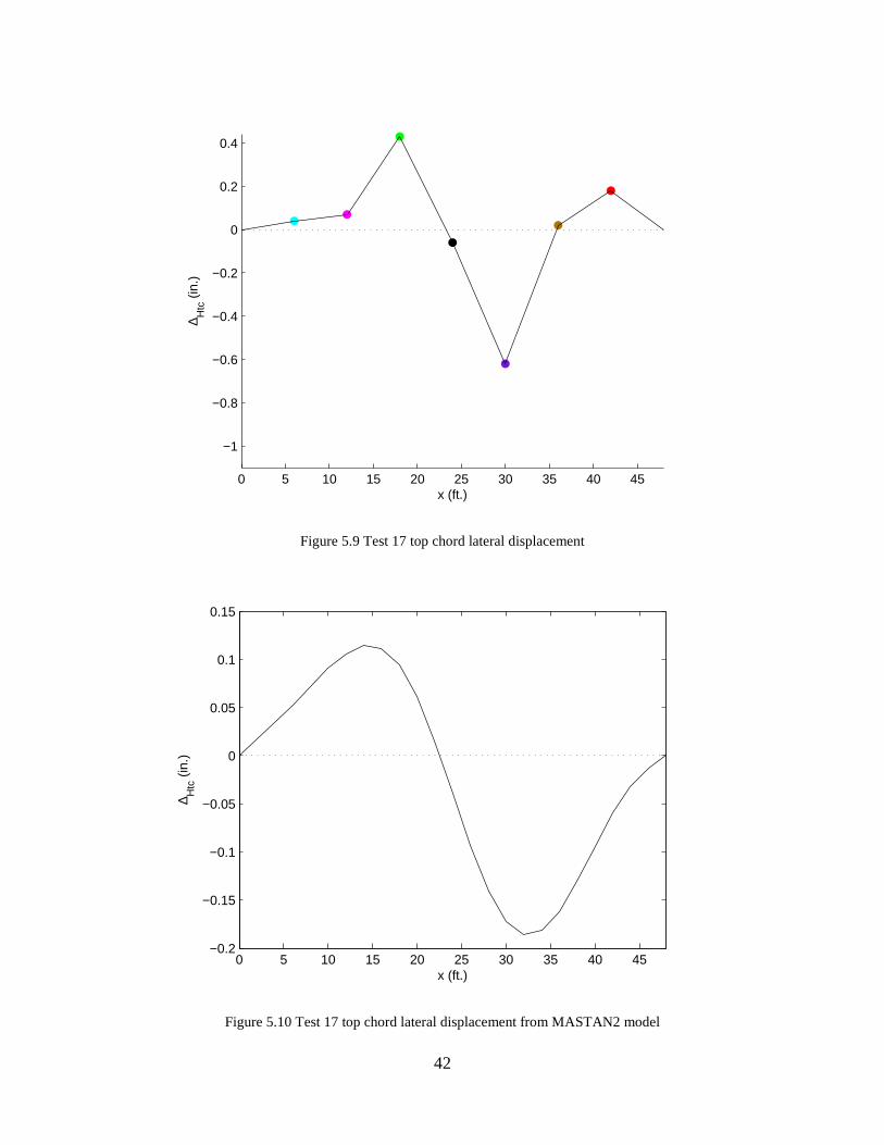
Figure 5.9 Test 17 top chord lateral displacement ........................................................................ 42
Figure 5.10 Test 17 top chord lateral displacement from MASTAN2 model .............................. 42
Figure 5.11 Test 18 top chord lateral displacement ...................................................................... 43
Figure 5.12 Test 18 top chord lateral displacement from MASTAN2 model .............................. 43
Appendix B
Figure B.1 Tensile test setup ......................................................................................................... 51
Figure B.2 Example engineering vs. true stress strain (for joist 1A) ............................................ 53
Figure B.3 0.2% offset example (for joist 1A) ............................................................................. 54
Figure B.4 Stress-strain relationship for Joist 2A ......................................................................... 55
Figure B.5 Stress-strain relationship for Joist 3B ......................................................................... 55
Figure B.6 Stress-strain relationship for Joist 4B ......................................................................... 55
Figure B.7 Stress-strain relationship for Joist 6A ......................................................................... 55

viii
Figure B.8 Stress-strain relationship for Joist 7B ......................................................................... 56
Figure B.9 Stress-strain relationship for Joist 8A ......................................................................... 56
Figure B.10 Stress-strain relationship for Joist 9A ....................................................................... 56
Figure B.11 Stress-strain relationship for Joist 10A ..................................................................... 56
Figure B.12 Stress-strain relationship for Joist 11B ..................................................................... 57
Figure B.13 Stress-strain relationship for Joist 12A ..................................................................... 57
Figure B.14 Stress-strain relationship for Joist 13B ..................................................................... 57
Figure B.15 Stress-strain relationship for Joist 14B ..................................................................... 57
Figure B.16 Stress-strain relationship for Joist 15A ..................................................................... 58
Figure B.17 Stress-strain relationship for Joist 16A ..................................................................... 58
Figure B.18 Stress-strain relationship for Joist 18B ..................................................................... 58
Figure B.19 Stress-strain relationship for Joist 25B ..................................................................... 58
Appendix C
Figure C.1 Cross-sectional dimensions of joist members (a) chord dimensions (b) web member
dimensions .................................................................................................................................... 60
Appendix F
Figure F.1 Joist dimensional inputs for Matlab ............................................................................ 86
Figure F.2 Elevation of a typical joist showing web member “groups” ....................................... 87
Figure F.3 Cross-sectional dimensions of joist members (a) chord dimensions (b) web member
dimensions .................................................................................................................................... 88
Figure F.4 Number of cross-sectional elements for a typical top chord angle ............................. 89
Figure F.5 Flowchart describing the process of finite element model generation ........................ 97

ix
List of Tables
Table 3.1 MASTAN2 to Exact Solution Comparison .................................................................. 20
Table 3.2 Exact to Approximate Solution Comparison ................................................................ 21
Table 4.1 Roof Stiffness Values ................................................................................................... 27
Table 5.1 As-tested and predicted roof stiffness and joist capacity .............................................. 35
Table 5.2 As-tested and predicted 24K4 joist capacity including bridging, Pcre calculated with
Eq. (2-4) ........................................................................................................................................ 35

1
Chapter 1 Introduction
The goal of this project was to develop a prediction method to determine the capacity of
an open web joist laterally supported by a standing seam roof system. Laboratory tests were
performed at Virginia Tech that evaluated the roof system variables to determine the influence of
each on the lateral restraint provided to the joists; the variables tested were clip height, insulation
thickness, presence of a thermal block, number bridging rows, chord size, and loading condition
(top or bottom chord) (Fehr 2012; Fehr et al. 2012). The goal of this research was to use the data
collected in the laboratory experiments to create a prediction method that could be used to
determine roof capacity.
Open-web steel joists are a staple of modern metal building construction. These joists
typically span over 40 ft. between primary portal frames, supporting a roof skin that serves as the
barrier to rain, snow, and wind. A common type of metal building roofing system supported by
open-web joists is the standing seam roof (Figure 1.1). Flexible clips are through-fastened along
the joist top chord and then the two edges of a metal roof panel are plastically folded with a
special seaming machine around the flexible clips, forming a watertight seal.
The standing seam clips are designed to accommodate roof elongation and contraction
from changes in temperature while still providing vertical support to the roof. Because the clips
are through-fastened to the top chord, they can provide some lateral bracing if the roof panels are
properly anchored to the eave and ridge. The roof panels can also envelop or “hug” the top
chord under gravity loads, providing additional lateral restraint. A common question asked by
joist manufacturers and metal building engineers is “How much top chord lateral support is

2
provided by a standing seam roof and can this lateral bracing be counted on in the flexural design
of a joist?”
Figure 1.1 Standing seam roof supported by an open-web joist
There is clear experimental evidence that a standing seam roof can provide partial lateral
restraint to a joist top chord. Holland and Murray (1983) evaluated the influence of standing
seam clip type, top chord size, and bridging location on joist capacity using a vacuum chamber.
Similar tests by Sherman and Fisher (1997) demonstrated that joist capacity decreased with
increasing clip height because as clip height increases, the lateral stiffness of the clip decreased
and the higher offset of the roof from the top chord reduced the “hugging” effect.
The laboratory tests performed at Virginia Tech (Fehr 2012; Fehr et al. 2012) showed
that standing seam roof systems without bridging have capacities very similar to those that
contain two and four rows of bridging. This shows that standing seam roofs without bridging are
capable of providing adequate lateral restraint to develop flexural capacities equivalent to
standing seam roof systems that use bridging. In addition, it was shown that both exclusion of
thermal blocks, and an increase in clip height decrease the flexural capacity of the system. It was
also shown that an increase in top chord size will increase the amount of top chord envelopment,
increasing the roof stiffness and joist capacity.
Clip Joist Top Chord
Roof PanelY
XZA
A
Z
Y
Section A-A

3
Sherman and Fisher emphasize in their paper that the standing seam panel must be
soundly connected to stiff eave and ridge members to ensure that the lateral bracing forces have a
load path to the primary framing. They measured these bracing forces in their tests on a two-
joist system and used the experimental results to validate engineering expressions motivated by
Winter (1958) for predicting required roof panel capacity. Sherman and Fisher point out that for
multiple joists the required bracing force provided by the roof is cumulative and that for sloped
roofs the gravity load in the direction of the bracing forces should also be considered in the total
demand.
One of the only existing analytical capacity prediction methods for joists braced by a
standing seam roof was developed by Hodge (1986), a master’s degree student advised by
Professor Theodore Galambos. Hodge and Galambos treated the joist top chord as a column
with an initial geometric imperfection, discrete springs at the clip locations (the hugging was not
considered), discrete supports at the bridging lines, and a parabolically varying axial load.
Second order elastic-plastic analysis of the column (joist top chord) was conducted by solving
simultaneous slope deflection equations describing moment equilibrium at nodes along the
column, where the node locations were at each clip (spring) location, bridging line, and end
support. Hodge compared his capacity predictions to the Holland and Murray (1983) tests,
however the validation was deemed unsatisfactory because of the lack of sweep imperfection
measurements in the experiments. Also, Hodge mentions that the Fortran program used to solve
the second-order analysis was quite slow.
This report builds on Hodge and Galambos’s analytical model to provide a general
strength prediction method for open-web steel joists braced by a standing seam roof. The
prediction method utilized classical stability solutions, modern structural analysis tools, and

4
existing code equations. Specifically, the existing AISC column curve is used to predict top
chord capacity using closed formed equations for the critical elastic buckling load of the top
chord including roof stiffness and bridging. A protocol for approximating the roof stiffness is
outlined that uses vacuum chamber test data and second order elastic analysis in a structural
analysis program (e.g., MASTAN2, SAP2000, RISA2D). The strength prediction method is
verified with a small set of recent experiments. More validation is needed though and the author
is hopeful that others will conduct similar tests to confirm the generality of the strength
prediction approach described in the following sections.

5
Chapter 2 Strength Prediction Approach
2.1 Introduction
The pressure load applied to the roof system can be broken down into a force couple
where the top chord of the joist is in compression while the bottom chord of the joist is in
tension. The axial load increases parabolically from zero at the end of each joist to a maximum at
midspan, and the standing seam roof provides adequate stiffness to allow each joist to be
supported as a column on an elastic foundation. The controlling mode of failure is out of plane
buckling of the top chord, this failure mode can be seen in Figure 2.1 and Figure 2.2.
Figure 2.1 Test 1 buckled shape
Figure 2.2 Test 2 buckled shape
As stated previously, the roof stiffness comes from two sources; the first is clip friction
created when the roof is seamed; the second is from top chord envelopment or “hugging” under a
uniform roof load; Figure 2.3 shows the two sources of roof stiffness.

6
(a)
(b)
Figure 2.3 roof stiffness sources (a) from clip friction and (b) from top chord envelopment or “hugging”
Because the top chord acts as a column (Figure 2.1) the existing column curve
represented in Chapter E of the AISC Specification, “Design of Members for Compression”, can
be used to predict joist capacity (AISC 2011). Figure 2.4 shows the column curve for a 24K4
joist top chord.
Figure 2.4 AISC column curve for 24K4 joists based on AISC Chapter E equations
The traditional AISC slenderness parameter kL/r was replaced with the equivalent
slenderness parameter (Py/Pcre)0.5 which is more frequently used to describe cold formed steel;
0 50 100 150 200 250 3000
10
20
30
40
50
60
Pn (
kip)
kL/r

7
these two slenderness parameters are equivalent, as shown in Appendix A. By using this
slenderness parameter the problem was simplified into determining the yield load and critical
elastic buckling load to predict capacity.
Top chord capacity was determined for each test performed during the laboratory
experiments using the models and measurements that were consistent with that test, a Microsoft
Excel spreadsheet was used to perform the necessary calculations and determine the capacity of
each top chord which could then be compared to the experimental capacity, equations used
within the spreadsheet are described below.
The column slenderness parameter can be described with the equation:
cre
yc P
P=λ
(2-1)
Where λc is the column slenderness parameter, Pcre is the critical elastic buckling load as
determined from an eigenbuckling analysis, and Py is the yield load of the top chord as
determined from the tensile coupon tests.
For an open-web joist partially braced by a standing seam roof and failing by lateral
buckling of the top chord (Figure 2.5), ultimate capacity, Pn, is approximated with the AISC
column curve equations, reformatted such that the global buckling slenderness, kL/r, is
represented instead as λc=(Py/Pcre)0.5 (Eq. (2-1)), see Appendix A for a proof that these two
slenderness values are equivalent
for λc≤1.5
for λc>1.5 (2-2)
8
where Py = AFy , A is the gross cross-sectional area of the top chord, Fy is the top chord steel
yield stress, and Pcre is the critical elastic buckling load of the joist top chord. The column curve
represented in Eq. (2-2) is used in both hot-rolled steel (AISC) and cold-formed steel (AISI)
codes, and therefore this proposed strength prediction method is applicable to top chord angles
made from either material. The calculation of Pcre can be performed with an elastic eigen-
buckling analysis in a structural analysis program, for example, MASTAN2 (MASTAN2/version
3.3) or SAP2000 (SAP2000/Advanced version 14.0.0) with the same models shown in Figure 2.5
except without an initial imperfection and with or without intermediate bridging lines and
including the parabolically varying axial load along the top chord.
Two methods are presented that allow for determining the capacity of the standing seam
roof system. The first uses structural analysis software to run an eigenbuckling analysis of top
chord models while the second method is an elastic buckling closed form solution that uses
simplified equations to calculate top chord slenderness and predict capacity. The first method is
to build a structural analysis model of the joist top chord, including discrete springs at bridging
locations with a parabolically varying axial load, and perform an eigenbuckling analysis to
determine the critical elastic buckling load; which is then used to determine top chord capacity.
This method requires access to structural analysis software and some training in finite element
modeling. The second method uses approximate hand solutions to predict the critical elastic
buckling load of the top chord and column slenderness.

9
2.2 Strength prediction using a full top chord mode l to determine Pcre
2.2.1 Strength prediction using eigenbuckling analy sis to determine Pcre
The first prediction method uses the full top chord length; this system is modeled as a
column with a parabolically-varying axial load supported on an elastic foundation. The top
chord is assumed to act as a singly-symmetric member with the two angles that comprise the top
chord acting together (they are typically welded together every 24 in.) and therefore flexural-
torsional buckling comprises two of the three buckling modes when solving the classic cubic
buckling equation (Chajes 1974). However, in this prediction method only flexural buckling is
considered because the diagonal and vertical web stems in combination with the roof are
assumed to suppress torsional deformation.
(a)
(b)
Figure 2.5 Top chord boundary conditions, loading, and lateral support (a) without and (b) with bridging lines
A uniformly distributed lateral spring with magnitude K (force/length/length) simulates a
smeared effect of clip stiffness and hugging along the top chord. This is different from the
cre
K
EIy
P
X
Z
ΔZ
Parabolic
axial loadcre
K
EIy
P
ΔZ
Fixed in the Z-direction
at bridging locations

10
Hodge (1986) treatment where only the clip stiffness at discrete locations was considered in the
prediction.
For the prediction method the stiffness of the clips was determined, see Chapter 4, and an
equivalent elastic foundation stiffness (stiffness per unit length) was determined. The roof
stiffness was then input into a similar model but without an imperfection, while the parabolic
load remained. From this point an eigenbuckling buckling analysis was performed to determine
the critical elastic buckling load, see Chapter 4 for full details of the top chord model. The yield
load of the top chord was determined as discussed in Appendix B; this information was used
within the column curve equations to determine top chord capacity.
2.2.2 Closed form solution to the full top chord mo del
Approximate hand methods are also available to calculate Pcre. A closed form solution of
a joist without bridging is presented below; these solutions are derived in Chapter 3.
00.201702.042
+
=
YY
cre
EI
KL
EI
LP
for 311
4
≤YEI
KL
55.630302.042
+
=
YY
cre
EI
KL
EI
LP
for 3874311
4
≤<YEI
KL
47.1340119.042
+
=
YY
cre
EI
KL
EI
LP
for 169603874
4
≤<YEI
KL
03.23000626.042
+
=
YY
cre
EI
KL
EI
LP
for 5000016960
4
≤<YEI
KL
67.32900427.042
+
=
YY
cre
EI
KL
EI
LP
for 8000050000
4
≤<YEI
KL
11
00.43500295.042
+
=
YY
cre
EI
KL
EI
LP
for 20000080000
4
≤<YEI
KL
80.68500165.042
+
=
YY
cre
EI
KL
EI
LP for 700000200000
4
≤<YEI
KL
(2-3)
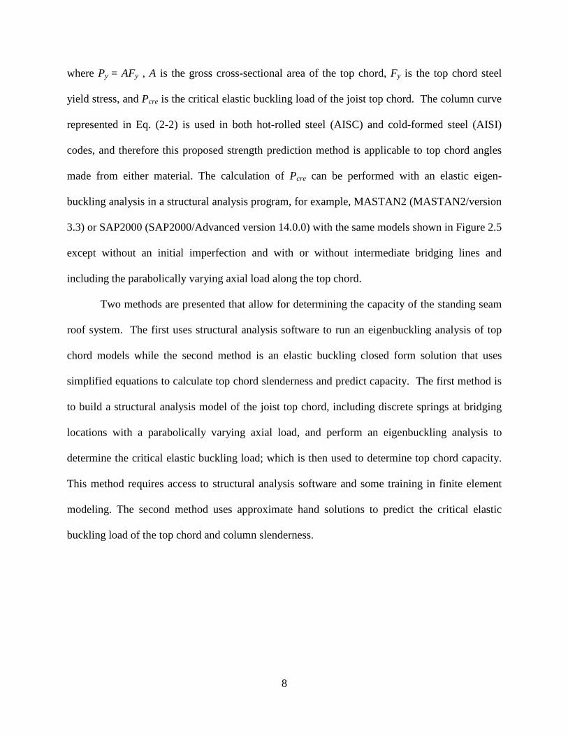
where L is the joist span. Eq. (2-3) is a linear curve fit to the slightly nonlinear exact solution
shown in Figure 2.6. Eq. (2-3) can be used to determine Pcre before using Eq. (2-2) to determine
top chord capacity.
Figure 2.6 Flexural column buckling on an elastic foundation with a parabolically varying axial load
2.3 Simplified method for roof systems with bridgin g
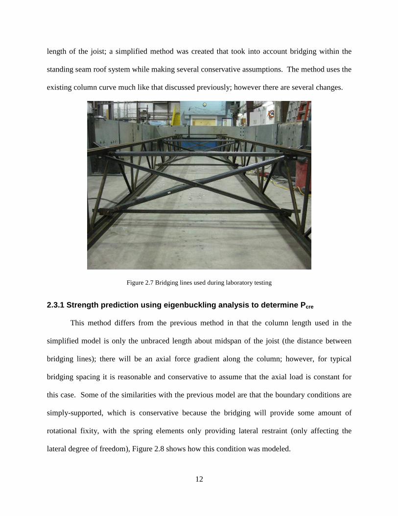
Bridging is commonly used in standing seam roof systems for erection as well as stability
purposes, an example of bridging can be found in Figure 2.7. It is necessary to include bridging
for erection purposes even if the standing seam roof system provides full bracing along the
0 1 2 3 4 5 6 7
x 105
0
200
400
600
800
1000
1200
1400
1600
1800
2000
Approximate solution
Exact solution
Y
cre
EI
LP 2
311
3874
16960
50000
80000 200000 700000
Pcre
L K
EIy
Parabolic
Axial
Load
YEI
KL4
12
length of the joist; a simplified method was created that took into account bridging within the
standing seam roof system while making several conservative assumptions. The method uses the
existing column curve much like that discussed previously; however there are several changes.
Figure 2.7 Bridging lines used during laboratory testing
2.3.1 Strength prediction using eigenbuckling analy sis to determine Pcre
This method differs from the previous method in that the column length used in the
simplified model is only the unbraced length about midspan of the joist (the distance between
bridging lines); there will be an axial force gradient along the column; however, for typical
bridging spacing it is reasonable and conservative to assume that the axial load is constant for
this case. Some of the similarities with the previous model are that the boundary conditions are
simply-supported, which is conservative because the bridging will provide some amount of
rotational fixity, with the spring elements only providing lateral restraint (only affecting the
lateral degree of freedom), Figure 2.8 shows how this condition was modeled.

13
Figure 2.8 Top chord boundary conditions, loading, and lateral support for the simplified (bridging) model
The roof stiffness from the previous model was used and the same process was
implemented to determine the top chord capacity for roof systems that use bridging. Pcre can be
determined as described in the previous section, by using a structural analysis program to model
the joist top chord as shown in Figure 2.8 and performing an eigenbuckling analysis.
2.3.2 Closed form solution to the simplified top ch ord model
Alternatively, a closed-form solution was derived to determine the top chord critical
elastic buckling load:
YY
cre
EI
KL
EI
LP
87.987.9
42
+=
for 3894
≤YEI
KL
YY
cre
EI
KL
EI
LP
48.3948.39
42
+=
for 35073894
≤<YEI
KL
YY
cre
EI
KL
EI
LP
83.8883.88
42
+=
for 1403035074
≤<YEI
KL
YY
cre
EI
KL
EI
LP
9.1579.157
42
+=
for 38964140304
≤<YEI
KL
cre
K
EIy
P
ΔZ
Axial Load
X
Z Lb = bridging distance
14
YY
cre
EI
KL
EI
LP
7.2467.246
42
+=
for 87670398644
≤<YEI
KL (2-4)
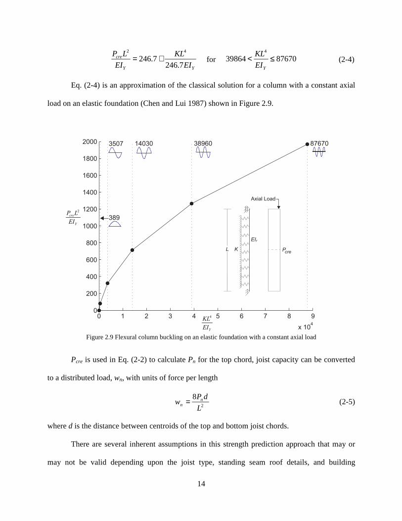
Eq. (2-4) is an approximation of the classical solution for a column with a constant axial
load on an elastic foundation (Chen and Lui 1987) shown in Figure 2.9.
Figure 2.9 Flexural column buckling on an elastic foundation with a constant axial load
Pcre is used in Eq. (2-2) to calculate Pn for the top chord, joist capacity can be converted
to a distributed load, wn, with units of force per length
2
8
L
dPw n
n = (2-5)
where d is the distance between centroids of the top and bottom joist chords.
There are several inherent assumptions in this strength prediction approach that may or
may not be valid depending upon the joist type, standing seam roof details, and building
0 1 2 3 4 5 6 7 8 9
x 104
0
200
400
600
800
1000
1200
1400
1600
1800
2000
YEI
KL4
Y
cre
EI
LP 2
Pcre
L K
EIy
Axial Load
389
140303507 38960 87670

15
boundary conditions. Catenary tension in the top chord is ignored which is most likely a
conservative assumption. Downward local bending of the top chord caused by concentrated
forces at the clip locations is ignored. A P-M interaction equation could be employed if there is
concern that the web stem spacing is too large. The standing seam roof is assumed to be able to
provide the distributed spring stiffness K and to have the capacity to carry the associated bracing
forces. A procedure for approximating K and the bracing force demand with a standard vacuum
chamber test and computer analysis is presented in Chapter 4.
16
Chapter 3 Fourth Order Linear Homogeneous Differential Equation Solution
3.1 Solution derivation – Parabolically varying loa d
To further check the prediction method outlined previously another method was created
using structural stability concepts. Dr. Raymond H. Plaut of Virginia Tech created a solution
using the computer program Mathematica that described the top chord as a simply-supported
column on an elastic foundation loaded with a parabolically varying axial compressive load
using a fourth-order linear homogeneous differential equation. The roof stiffness K, see Chapter
4, was input as the elastic foundation stiffness, and laboratory joist test properties, such as cross-
sectional area and top chord moment of inertia, were used when determining the capacity of the
top chord.
3.1.1 Differential equation derivation
Boundary conditions within the solution included zero deflection and zero moment at the
ends of the column, corresponding to:
0)(
0)0(
0)(
0)0(
=′′=′′
==
LEIY
EIY
LY
Y
(3-1)
Where Y represents the lateral deflection of the top chord, Y’’EI represents the moment in
the top chord, and L represents the clear span distance of the joist.
Load was applied axially as a compressive load continuously along the length of the
column varying parabolically; the load was expressed with Eq. (3-2).
−
=L
X
L
XPXP 14)( 0
(3-2)
17
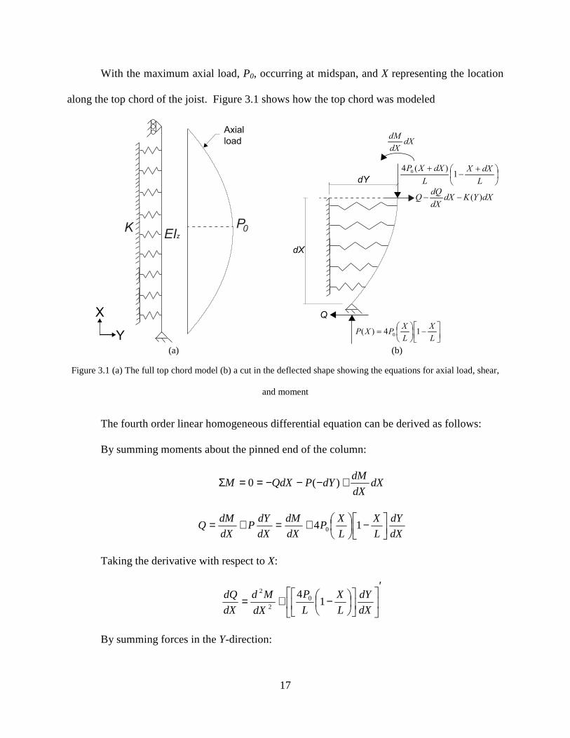
With the maximum axial load, P0, occurring at midspan, and X representing the location
along the top chord of the joist. Figure 3.1 shows how the top chord was modeled
(a)
(b)
Figure 3.1 (a) The full top chord model (b) a cut in the deflected shape showing the equations for axial load, shear,
and moment
The fourth order linear homogeneous differential equation can be derived as follows:
By summing moments about the pinned end of the column:
dXdX
dMdYPQdXM +−−−==Σ )(0
dX
dY
L
X
L
XP
dX
dM
dX
dYP
dX
dMQ
−
+=+= 14 0
Taking the derivative with respect to X:
′
−+=dX
dY
L
X
L
P
dX
Md
dX
dQ1
4 02
2
By summing forces in the Y-direction:
0KEIz
P
Y
X
Axial
load
dX
Q
+−
+
L
dXX
L
dXXP1
)(4 0
−
=
L
X
L
XPXP 14)( 0
dX
dX
dM
dY
dXYKdXdX
dQQ )(−−

18
dXYKdXdX
dQQQFY )(0 −−+−==Σ
)()( YKdX
dQYK
dX
dQ −=→=−
2
2
2
2
)(dX
YdP
dX
MdYK +=−
0)(14 0
2
2
=+′
−+ YKdX
dY
L
X
L
XP
dX
Md
Given that curvature can be described with the following relationship:
2
2
dX
Yd
EI
M =
The substitution can then be made to arrive at the final equation:
014 0 =+′
′
−
+′′′′ KYYL
X
L
XPYEI
(3-3)
3.1.2 Solution using nondimensional quantities
The solution was simplified for use in Mathematica by using non-dimensional quantities
for all variables as shown below:
L
Xx =
L
Yy =
EI
KLk
4
= (3-4)
Where x and y are normalized by determining the percentage of the span can be
represented by the location along the top chord and top chord displacement respectively.
19
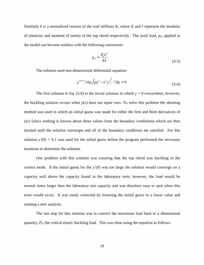
Similarly k is a normalized version of the roof stiffness K, where E and I represent the modulus
of elasticity and moment of inertia of the top chord respectively. The axial load, p0, applied to
the model can become unitless with the following conversion:
EI
LPp
20
0 = (3-5)
The solution used non-dimensional differential equation:
( ) 04 20 =+′′−′+′′′′ kyyxyxpy (3-6)
The first solution to Eq. (3-6) is the trivial solution in which y = 0 everywhere; however,
the buckling solution occurs when y(x) does not equal zero. To solve this problem the shooting
method was used in which an initial guess was made for either the first and third derivatives of
y(x) (since nothing is known about these values from the boundary conditions) which are then
iterated until the solution converges and all of the boundary conditions are satisfied. For this
solution y’(0) = 0.1 was used for the initial guess before the program performed the necessary
iterations to determine the solution.
One problem with this solution was ensuring that the top chord was buckling in the
correct mode. If the initial guess for the y’(0) was too large the solution would converge on a
capacity well above the capacity found in the laboratory tests; however, the load would be
several times larger than the laboratory test capacity and was therefore easy to spot when this
error would occur. It was easily corrected by lowering the initial guess to a lower value and
running a new analysis.
The last step for this solution was to convert the maximum load back to a dimensional
quantity, P0, the critical elastic buckling load. This was done using the equation as follows:
20
20
0 L
EIpP =
(3-7)
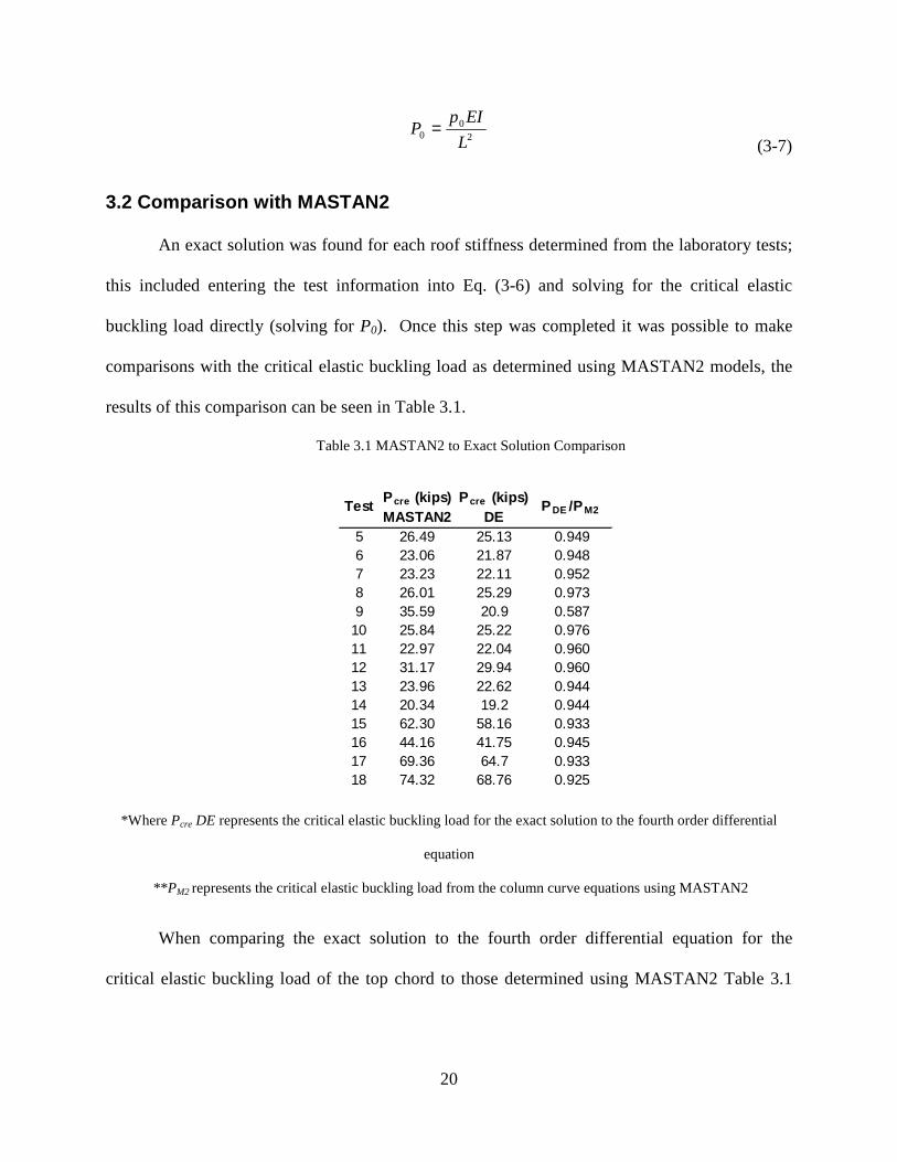
3.2 Comparison with MASTAN2
An exact solution was found for each roof stiffness determined from the laboratory tests;
this included entering the test information into Eq. (3-6) and solving for the critical elastic
buckling load directly (solving for P0). Once this step was completed it was possible to make
comparisons with the critical elastic buckling load as determined using MASTAN2 models, the
results of this comparison can be seen in Table 3.1.
Table 3.1 MASTAN2 to Exact Solution Comparison
*Where Pcre DE represents the critical elastic buckling load for the exact solution to the fourth order differential
equation
** PM2 represents the critical elastic buckling load from the column curve equations using MASTAN2
When comparing the exact solution to the fourth order differential equation for the
critical elastic buckling load of the top chord to those determined using MASTAN2 Table 3.1
TestPcre (kips) MASTAN2
Pcre (kips) DE
PDE /PM2
5 26.49 25.13 0.9496 23.06 21.87 0.9487 23.23 22.11 0.9528 26.01 25.29 0.9739 35.59 20.9 0.587
10 25.84 25.22 0.97611 22.97 22.04 0.96012 31.17 29.94 0.96013 23.96 22.62 0.94414 20.34 19.2 0.94415 62.30 58.16 0.93316 44.16 41.75 0.94517 69.36 64.7 0.93318 74.32 68.76 0.925

21
shows that the fourth order differential equation prediction tends to be relatively close to Pcre
determined using MASTAN2, while also being slightly more conservative.
It should be noted that the values in Table 3.1 do not include tests 1-4. This is because
the solution to this problem does not include discrete supports at bridging locations and thus the
effect of bridging is not included in the model. It would not be appropriate to include the first
four tests in this analysis because these tests would not be modeled correctly.
3.3 Comparison with the idealized linear solution
It can be seen in Figure 2.6 that there is a discrepancy between the exact solution (red
dashed line) to the fourth order differential equation and those idealized with Eq. (2-3) (black
solid line). It is therefore necessary to compare the closed form solution to the exact solution,
Table 3.2 shows this comparison.
Table 3.2 Exact to Approximate Solution Comparison
*Where Pn DE represents the top chord capacity as predicted by the exact solution to the fourth order differential
equation
** Pn Eq. (2-3) represents the top chord capacity as predicted by Eq. (2-3)
TestPn (kips)
DEPn (kips) Eq. (2-3)
PDE /Pn
5 21.3 20.9 1.026 19.1 18.5 1.037 19.3 18.7 1.038 21.8 20.8 1.049 18.3 18.5 0.9910 21.6 20.8 1.0411 19.3 18.6 1.0312 23.5 24.4 0.9613 19.6 19.1 1.0314 16.8 16.3 1.0315 42.6 42.3 1.0116 35.1 34.2 1.0317 53.4 52.2 1.0218 56.0 54.7 1.02

22
It can be seen in Table 3.2 that the approximate solution determined using Eq. (2-3) is
close to the exact solution adding a reasonable amount of conservatism (about three percent) to
the prediction.

23
Chapter 4 Determination of Roof Stiffness
4.1 Procedure
The lateral stiffness provided by the standing seam roof to the top chord is influenced by
many variables, including clip type, clip height, the presence of insulation between the panel and
the joist, panel profile and gage, and the failure pressure which for a lower capacity joist will not
cause hugging, or for a stronger joist, may result in significant hugging.
This new procedure for approximating K employs experimental data from a vacuum box
test for systems without or with bridging in combination with a second order elastic analysis of
the top chord performed in a structural analysis computer program (e.g., MASTAN2, SAP2000,
RISA2D). The idea is to measure the lateral displacement of the joist top chord relative to the
roof at multiple points along the span, and then to use a structural analysis program to solve for
the K that results in the best match between the displaced shape in the structural analysis and the
measured displaced shape of the joist.
The first step is to start with a vacuum box test and measure the displacement of the joists
relative to the standing seam roof near failure as shown in Figure 4.1 (a). To be consistent with
the assumptions in the prediction method that the roof eave and rafter boundary conditions are
rigid, the roof edges should be reinforced with through-fastened angles and also braced at
intermediate points along the span, for example, as shown in Figure 4.1 (b). The initial sweep
imperfection shape and magnitudes along the span should be measured and recorded. It is
recommended that three tests be performed to ensure that statistical variations can be averaged in
the final determination of K.

24
Once the experiments are complete, a computer model is constructed where the top chord
is simulated as a pinned-pinned column with distributed springs along its length (similar to
Figure 2.5). The measured imperfection shape and magnitudes are imposed on the initial
geometry of the model (so if three tests were performed then there would be three models), and a
parabolically varying axial load is applied. A second order elastic analysis of the top chord
including the imperfections and measured joist top chord section properties can then be run
multiple times while varying the spring stiffness K . The roof stiffness K that minimizes the
difference between the predicted and measured displacements from the experiment is averaged
between the three tests and then used in Eq. (2-3), Eq. (2-4), or in an eigenbuckling analysis.
The total bracing force demand can also be approximated by adding up all the spring forces in
the model. It is essential when employing the joist strength prediction method described herein
that K be experimentally determined for each combination of roof system variables (e.g., clip
height, panel profile, insulation thickness).
(a)
(b)
Figure 4.1 Vacuum box experiment details: (a) measurement of joist top chord relative to roof, and (b) proposed
roof bracing details
Position transducer (typ.)
West East
∆(relative to roof)+ +
Roof edge
reinforcement
(typ.)
Section A-A
A B
Pressure box walls
Joist (typ.) Roof braces
Roof edge reinforcement (typ.)
CL Bearings (typ.)
A
A

25
The roof stiffness was determined for each laboratory experiment performed. The clips
were modeled to allow for all of the stiffness provided from the standing seam roof system to be
grouped together at the clip locations. This was; however, an approximation of the roof stiffness
behavior because the lateral restraint provided from the roof system came from two sources,
clamping force and envelopment of the top chord by the roofing panels under load. It was
necessary to group the stiffness at the clip locations because there was no way to determine the
amount of stiffness provided by the clips and hugging separately from the test information, not to
mention modeling this condition was not possible in the programs used for analysis.
Once Matlab code was written to generate input files for MASTAN2 several models were
created. From these models, and as was suspected from the experimental tests, it was discovered
that the top chord behaved as a column loaded axially on an elastic foundation. This meant that
the stiffness provided from the standing seam roof system could be thought of as a stiffness per
length (force/length/length) measure rather than lumping the roof stiffness at the clip locations.
To confirm the model results additional wirepots were added to the experimental test setup to
measure lateral deflection along the length of the joist rather than just at midspan as was done
previously. Figure 5.1 through Figure 5.12, show the deflected shape of the top chord from the
experimental tests, as well as those predicted by the MASTAN2 models. These plots confirm
the theory that the top chord behaves as if the standing seam roof supported the joists as an
elastic foundation. Additionally, the figures in Appendix D show the deflected shapes from the
MASTAN2 models of tests one through twelve, which were not able to be compared to the test
deflected shapes because lateral displacements along the top chord were not recorded for these
tests.
26
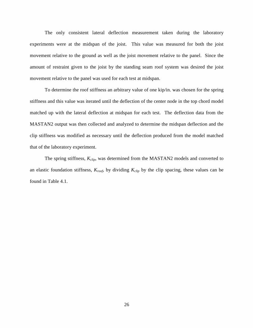
The only consistent lateral deflection measurement taken during the laboratory
experiments were at the midspan of the joist. This value was measured for both the joist
movement relative to the ground as well as the joist movement relative to the panel. Since the
amount of restraint given to the joist by the standing seam roof system was desired the joist
movement relative to the panel was used for each test at midspan.
To determine the roof stiffness an arbitrary value of one kip/in. was chosen for the spring
stiffness and this value was iterated until the deflection of the center node in the top chord model
matched up with the lateral deflection at midspan for each test. The deflection data from the
MASTAN2 output was then collected and analyzed to determine the midspan deflection and the
clip stiffness was modified as necessary until the deflection produced from the model matched
that of the laboratory experiment.
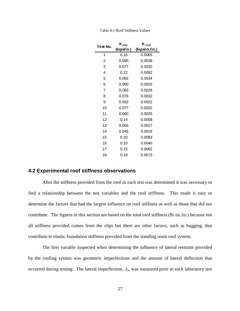
The spring stiffness, Kclip, was determined from the MASTAN2 models and converted to
an elastic foundation stiffness, Kroof, by dividing Kclip by the clip spacing, these values can be
found in Table 4.1.
27
Table 4.1 Roof Stiffness Values
4.2 Experimental roof stiffness observations
After the stiffness provided from the roof in each test was determined it was necessary to
find a relationship between the test variables and the roof stiffness. This made it easy to
determine the factors that had the largest influence on roof stiffness as well as those that did not
contribute. The figures in this section are based on the total roof stiffness (lb./in./in.) because not
all stiffness provided comes from the clips but there are other factors, such as hugging, that
contribute to elastic foundation stiffness provided from the standing seam roof system.
The first variable inspected when determining the influence of lateral restraint provided
by the roofing system was geometric imperfections and the amount of lateral deflection that
occurred during testing. The lateral imperfection, ∆z, was measured prior to each laboratory test
Test No.K clip
(kips/in.)K roof
(kips/in./in.)1 0.16 0.0065
2 0.090 0.0038
3 0.077 0.0032
4 0.22 0.0092
5 0.082 0.0034
6 0.060 0.0025
7 0.062 0.0026
8 0.076 0.0032
9 0.052 0.0022
10 0.077 0.0032
11 0.060 0.0025
12 0.14 0.0058
13 0.065 0.0027
14 0.045 0.0019
15 0.20 0.0083
16 0.10 0.0040
17 0.15 0.0062
18 0.18 0.0073

28
and was measured as the lateral distance between the edge at the end of the top chord and the top
chord edge at quarter points along the joist, and example can be found in Figure 4.2.
Figure 4.2 Example of how the top chord imperfection was measured
It was found that the lateral restraint of the roof was not influenced by the imperfection of
the joist; this conclusion makes logical sense because these two factors are independent of one
another and the elastic foundation stiffness caused by the influence of the clips should not vary
regardless of the imperfection magnitude of the joist. Figure 4.3 shows the effect of the
maximum imperfection on roof stiffness; this plot does not have any conclusive trends to it but is
organized in a more random configuration. Some of the groups of data points appear to have
trends in them; however, these are due to other common variables that are shared amongst them
and are not due to the effect of the imperfection magnitude.
Figure 4.3 Effect of the maximum sweep imperfect on roof stiffness
Δz
Top chord
0 0.2 0.4 0.6 0.8 1 1.21
2
3
4
5
6
7
8
9
10
∆z (in.)
Kro
of (
lb./i
n./in
.)
24K424K824K12
29
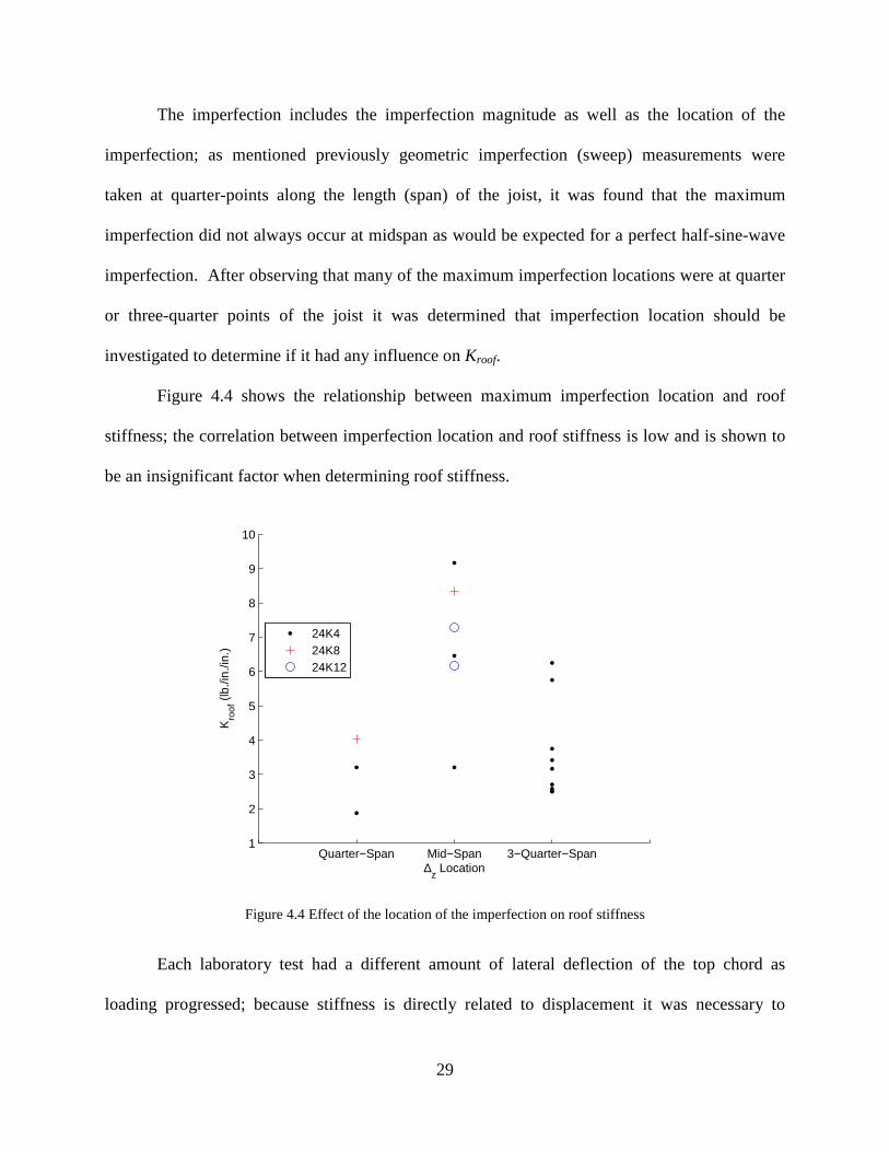
The imperfection includes the imperfection magnitude as well as the location of the
imperfection; as mentioned previously geometric imperfection (sweep) measurements were
taken at quarter-points along the length (span) of the joist, it was found that the maximum
imperfection did not always occur at midspan as would be expected for a perfect half-sine-wave
imperfection. After observing that many of the maximum imperfection locations were at quarter
or three-quarter points of the joist it was determined that imperfection location should be
investigated to determine if it had any influence on Kroof.
Figure 4.4 shows the relationship between maximum imperfection location and roof
stiffness; the correlation between imperfection location and roof stiffness is low and is shown to
be an insignificant factor when determining roof stiffness.
Figure 4.4 Effect of the location of the imperfection on roof stiffness
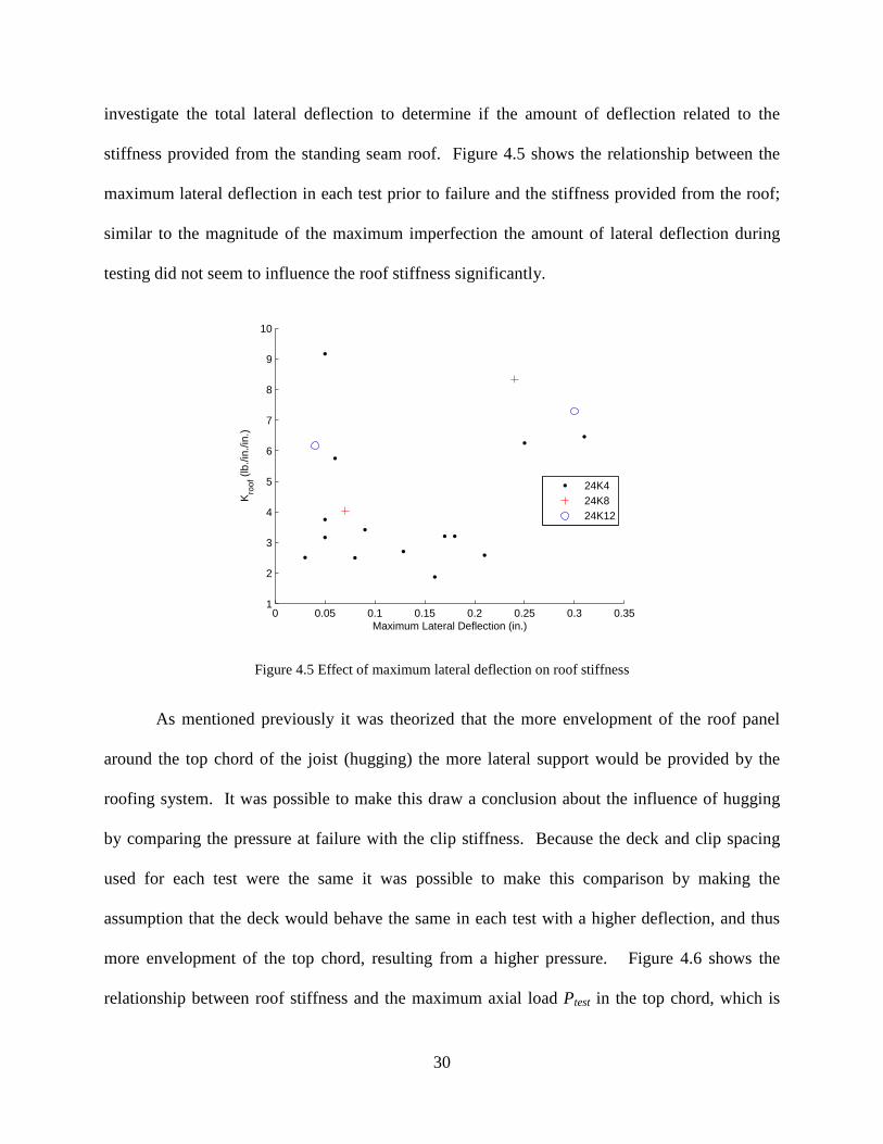
Each laboratory test had a different amount of lateral deflection of the top chord as
loading progressed; because stiffness is directly related to displacement it was necessary to
Quarter−Span Mid−Span 3−Quarter−Span1
2
3
4
5
6
7
8
9
10
∆z Location
Kro
of (
lb./i
n./in
.)
24K424K824K12
30
investigate the total lateral deflection to determine if the amount of deflection related to the
stiffness provided from the standing seam roof. Figure 4.5 shows the relationship between the
maximum lateral deflection in each test prior to failure and the stiffness provided from the roof;
similar to the magnitude of the maximum imperfection the amount of lateral deflection during
testing did not seem to influence the roof stiffness significantly.
Figure 4.5 Effect of maximum lateral deflection on roof stiffness
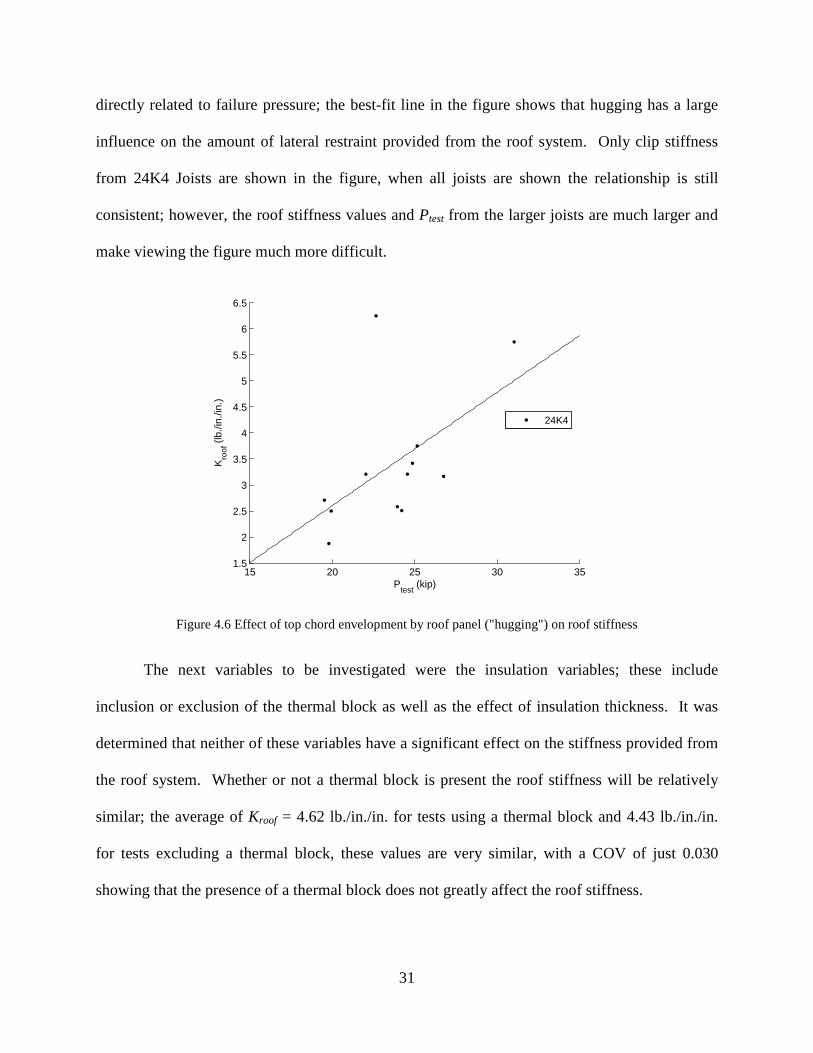
As mentioned previously it was theorized that the more envelopment of the roof panel
around the top chord of the joist (hugging) the more lateral support would be provided by the
roofing system. It was possible to make this draw a conclusion about the influence of hugging
by comparing the pressure at failure with the clip stiffness. Because the deck and clip spacing
used for each test were the same it was possible to make this comparison by making the
assumption that the deck would behave the same in each test with a higher deflection, and thus
more envelopment of the top chord, resulting from a higher pressure. Figure 4.6 shows the
relationship between roof stiffness and the maximum axial load Ptest in the top chord, which is
0 0.05 0.1 0.15 0.2 0.25 0.3 0.351
2
3
4
5
6
7
8
9
10
Maximum Lateral Deflection (in.)
Kro
of (
lb./i
n./in
.)
24K424K824K12
31
directly related to failure pressure; the best-fit line in the figure shows that hugging has a large
influence on the amount of lateral restraint provided from the roof system. Only clip stiffness
from 24K4 Joists are shown in the figure, when all joists are shown the relationship is still
consistent; however, the roof stiffness values and Ptest from the larger joists are much larger and
make viewing the figure much more difficult.
Figure 4.6 Effect of top chord envelopment by roof panel ("hugging") on roof stiffness
The next variables to be investigated were the insulation variables; these include
inclusion or exclusion of the thermal block as well as the effect of insulation thickness. It was
determined that neither of these variables have a significant effect on the stiffness provided from
the roof system. Whether or not a thermal block is present the roof stiffness will be relatively
similar; the average of Kroof = 4.62 lb./in./in. for tests using a thermal block and 4.43 lb./in./in.
for tests excluding a thermal block, these values are very similar, with a COV of just 0.030
showing that the presence of a thermal block does not greatly affect the roof stiffness.
15 20 25 30 351.5
2
2.5
3
3.5
4
4.5
5
5.5
6
6.5
Kro
of (
lb./i
n./in
.)
Ptest
(kip)
24K4

32
Figure 4.7 shows the influence of insulation thickness; the best-fit line in this plot shows
that a thicker insulation will result in less stiffness from the roofing system. It is unclear if the
insulation thickness has an effect on Kroof because the sample size is much smaller for the larger
insulation thickness, further testing is required to draw a strong conclusion about the effects of
insulation thickness on Kroof.
Figure 4.7 Effect of insulation thickness on roof stiffness
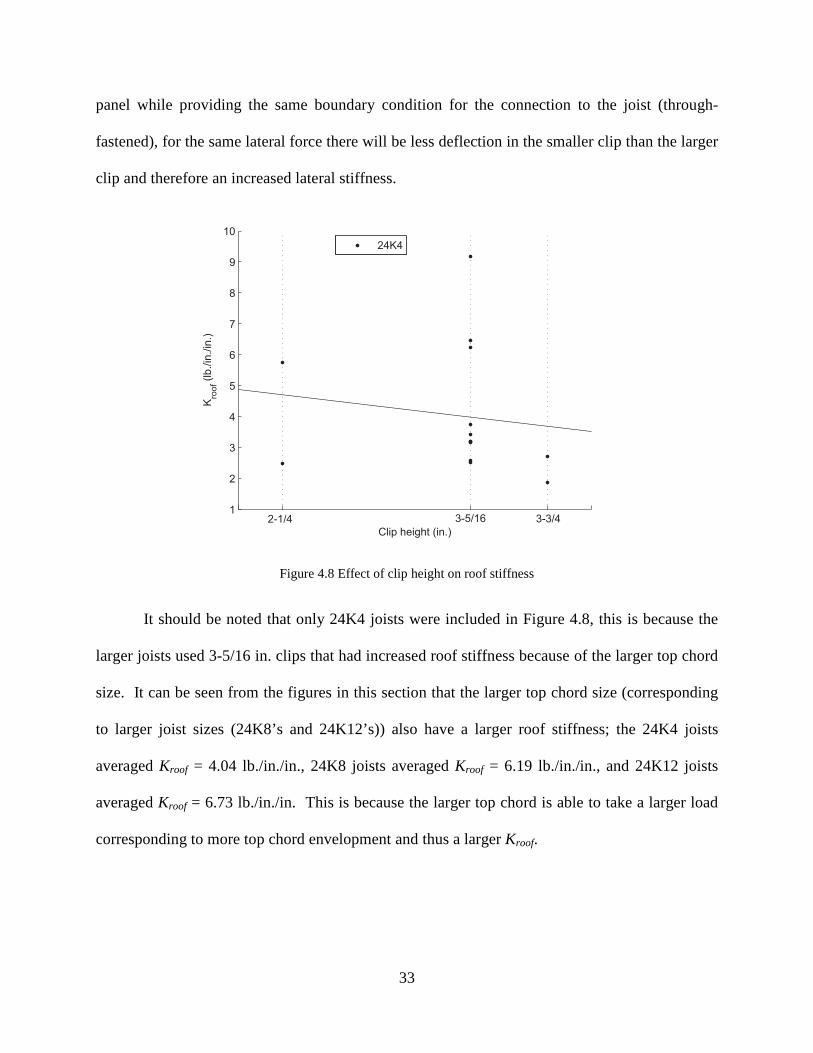
The last variable to investigate was the influence of clip height on the lateral stiffness
provided from the standing seam roof. Figure 4.8 shows the relationship between clip height and
Kroof; this plot shows that the smaller clip provides more lateral restraint from the roof system.
The reason for this increase is because of hugging as well as an increase in clip stiffness; a
smaller clip allows the roof panel to sit closer to the top chord of the joist, because the roof panel
is closer to the top chord it takes less deflection to envelope the top chord. Because envelopment
of the top chord comes at a lower load there is more hugging for a smaller clip than a larger clip
for two roof systems under the same load. Furthermore, the smaller clip will sit closer to the roof
2 4 61
2
3
4
5
6
7
8
9
10
Insulation Thickness (in.)
Kro
of (
lb./i
n./in
.)
24K4
33
panel while providing the same boundary condition for the connection to the joist (through-
fastened), for the same lateral force there will be less deflection in the smaller clip than the larger
clip and therefore an increased lateral stiffness.
Figure 4.8 Effect of clip height on roof stiffness
It should be noted that only 24K4 joists were included in Figure 4.8, this is because the
larger joists used 3-5/16 in. clips that had increased roof stiffness because of the larger top chord
size. It can be seen from the figures in this section that the larger top chord size (corresponding
to larger joist sizes (24K8’s and 24K12’s)) also have a larger roof stiffness; the 24K4 joists
averaged Kroof = 4.04 lb./in./in., 24K8 joists averaged Kroof = 6.19 lb./in./in., and 24K12 joists
averaged Kroof = 6.73 lb./in./in. This is because the larger top chord is able to take a larger load
corresponding to more top chord envelopment and thus a larger Kroof.
1
2
3
4
5
6
7
8
9
10
Clip height (in.)
Kro
of (
lb./in
./in
.)
24K4
2-1/4 3-5/16 3-3/4

34
Chapter 5 Test-to-Predicted Comparison
In order to validate the prediction method it was necessary to compare the test data with
the capacity predicted by the methods outlined in Chapter 2. For this process the maximum axial
load in each of the laboratory tests was calculated and this value was compared to the predicted
maximum axial load.
Past literature was reviewed that included standing seam roof tests similar to those
performed at Virginia Tech. It was desired to use the same prediction method outlined
previously for validation with these tests; however, it was found that either the testing procedure
differed too greatly or that measurements taken during testing did not provide enough
information to accurately analyze the behavior of the roof system. Therefore only data was
analyzed from information provided from the Virginia Tech tests.
5.1 Top chord test capacity vs. predicted capacity
A recent experimental program motivated the development of the prediction method
described in Chapter 2. The procedure was implemented to find the roof stiffness K and to
predict joist capacity for roof systems without and with bridging. The test results are compared
to predictions in Table 5.1 where the top chord critical elastic buckling load, Pcre, was calculated
with Eq. (2-4) for the tests without bridging and with eigenbuckling frame analysis in
MASTAN2 for the cases with bridging.
The test-to-predicted mean and COV for the results in Table 5.1 are 1.08 and 0.12
respectively, demonstrating the prediction method is viable for the conditions considered. The
roof stiffness K, derived with the iterative hybrid approach described in Chapter 4, increases with
decreasing clip height and increasing failure pressure. These trends in roof stiffness are
consistent with engineering intuition and with results from Sherman and Fisher (1996).
35
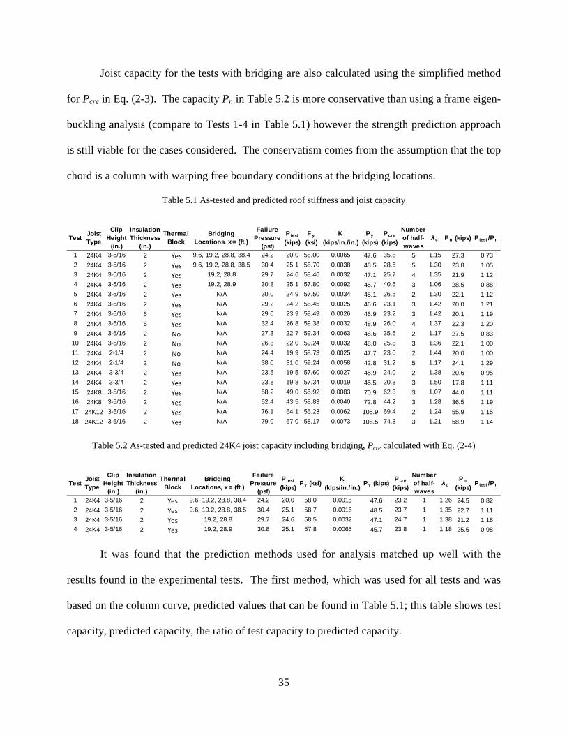
Joist capacity for the tests with bridging are also calculated using the simplified method
for Pcre in Eq. (2-3). The capacity Pn in Table 5.2 is more conservative than using a frame eigen-
buckling analysis (compare to Tests 1-4 in Table 5.1) however the strength prediction approach
is still viable for the cases considered. The conservatism comes from the assumption that the top
chord is a column with warping free boundary conditions at the bridging locations.
Table 5.1 As-tested and predicted roof stiffness and joist capacity
Table 5.2 As-tested and predicted 24K4 joist capacity including bridging, Pcre calculated with Eq. (2-4)
It was found that the prediction methods used for analysis matched up well with the
results found in the experimental tests. The first method, which was used for all tests and was
based on the column curve, predicted values that can be found in Table 5.1; this table shows test
capacity, predicted capacity, the ratio of test capacity to predicted capacity.
TestJoist Type
Clip Height
(in.)
Insulation Thickness
(in.)
Thermal Block
Bridging Locations, x= (ft.)
Failure Pressure
(psf)
P test
(kips)F y
(ksi)K
(kips/in./in.)Py
(kips)Pcre
(kips)
Number of half-waves
λ c Pn (kips) P test /Pn
1 24K4 3-5/16 2 Yes 9.6, 19.2, 28.8, 38.4 24.2 20.0 58.00 0.0065 47.6 35.8 5 1.15 27.3 0.73
2 24K4 3-5/16 2 Yes 9.6, 19.2, 28.8, 38.5 30.4 25.1 58.70 0.0038 48.5 28.6 5 1.30 23.8 1.05
3 24K4 3-5/16 2 Yes 19.2, 28.8 29.7 24.6 58.46 0.0032 47.1 25.7 4 1.35 21.9 1.12
4 24K4 3-5/16 2 Yes 19.2, 28.9 30.8 25.1 57.80 0.0092 45.7 40.6 3 1.06 28.5 0.88
5 24K4 3-5/16 2 Yes N/A 30.0 24.9 57.50 0.0034 45.1 26.5 2 1.30 22.1 1.12
6 24K4 3-5/16 2 Yes N/A 29.2 24.2 58.45 0.0025 46.6 23.1 3 1.42 20.0 1.21
7 24K4 3-5/16 6 Yes N/A 29.0 23.9 58.49 0.0026 46.9 23.2 3 1.42 20.1 1.19
8 24K4 3-5/16 6 Yes N/A 32.4 26.8 59.38 0.0032 48.9 26.0 4 1.37 22.3 1.20
9 24K4 3-5/16 2 No N/A 27.3 22.7 59.34 0.0063 48.6 35.6 2 1.17 27.5 0.83
10 24K4 3-5/16 2 No N/A 26.8 22.0 59.24 0.0032 48.0 25.8 3 1.36 22.1 1.00
11 24K4 2-1/4 2 No N/A 24.4 19.9 58.73 0.0025 47.7 23.0 2 1.44 20.0 1.00
12 24K4 2-1/4 2 No N/A 38.0 31.0 59.24 0.0058 42.8 31.2 5 1.17 24.1 1.29
13 24K4 3-3/4 2 Yes N/A 23.5 19.5 57.60 0.0027 45.9 24.0 2 1.38 20.6 0.95
14 24K4 3-3/4 2 Yes N/A 23.8 19.8 57.34 0.0019 45.5 20.3 3 1.50 17.8 1.11
15 24K8 3-5/16 2 Yes N/A 58.2 49.0 56.92 0.0083 70.9 62.3 3 1.07 44.0 1.11
16 24K8 3-5/16 2 Yes N/A 52.4 43.5 58.83 0.0040 72.8 44.2 3 1.28 36.5 1.19
17 24K12 3-5/16 2 Yes N/A 76.1 64.1 56.23 0.0062 105.9 69.4 2 1.24 55.9 1.15
18 24K12 3-5/16 2 Yes N/A 79.0 67.0 58.17 0.0073 108.5 74.3 3 1.21 58.9 1.14
TestJoist Type
Clip Height
(in.)
Insulation Thickness
(in.)
Thermal Block
Bridging Locations, x = (ft.)
Failure Pressure
(psf)
P test
(kips)F y (ksi)
K (kips/in./in.)
Py (kips)Pcre
(kips)
Number of half-waves
λ cPn
(kips)P test /Pn
1 24K4 3-5/16 2 Yes 9.6, 19.2, 28.8, 38.4 24.2 20.0 58.0 0.0015 47.6 23.2 1 1.26 24.5 0.82
2 24K4 3-5/16 2 Yes 9.6, 19.2, 28.8, 38.5 30.4 25.1 58.7 0.0016 48.5 23.7 1 1.35 22.7 1.11
3 24K4 3-5/16 2 Yes 19.2, 28.8 29.7 24.6 58.5 0.0032 47.1 24.7 1 1.38 21.2 1.16
4 24K4 3-5/16 2 Yes 19.2, 28.9 30.8 25.1 57.8 0.0065 45.7 23.8 1 1.18 25.5 0.98

36
Values in Table 5.2 show that the prediction from the column curve is generally
conservative and reasonably accurate. Values for the test capacity ratio, Ptest/Pn, greater than 1.0
show that the failure load is greater than the predicted capacity and is therefore conservative, this
is true for majority of the test capacity ratios and those that are less than 1.0 generally do not
deviate from 1.0 by a very large margin. It was expected that predictions would be on the
conservative side considering that many of the assumptions made in the prediction method were
conservative.
It can be seen from Table 5.1 that the only test with a capacity ratio well below 1.0 is
from test 1. During laboratory testing there was a slip in the roof system prior to failure that is
believed to have made the joist fail at a much lower load than expected, therefore Ptest is low for
this test making Ptest/Pn lower than normal. The slip that occurred in Test 1 was not observed in
any other tests and is thought to have occurred due to a mistake made while assembling the test
and is not typical standing seam roof behavior.
The next prediction method to be analyzed was the simplified method that was used on
roof systems that contained bridging. This system used the same prediction method using the
column curve; however, the critical buckling load was determined with a MASTAN2 model with
a constant axial load and length equivalent to the central bridging distance, see Chapter 2 for
more details; the capacity prediction for this method can be seen in Table 5.2. The strength
prediction for this method is once again conservative as well as accurate; the values are more
conservative than those values found in Table 5.1 due to the additional conservative assumptions
made. The values for the load capacity ratio are higher than those found previously; with the
only non-conservative value occurring in Test 1 where there were problems during the laboratory
test, as discussed previously.
37
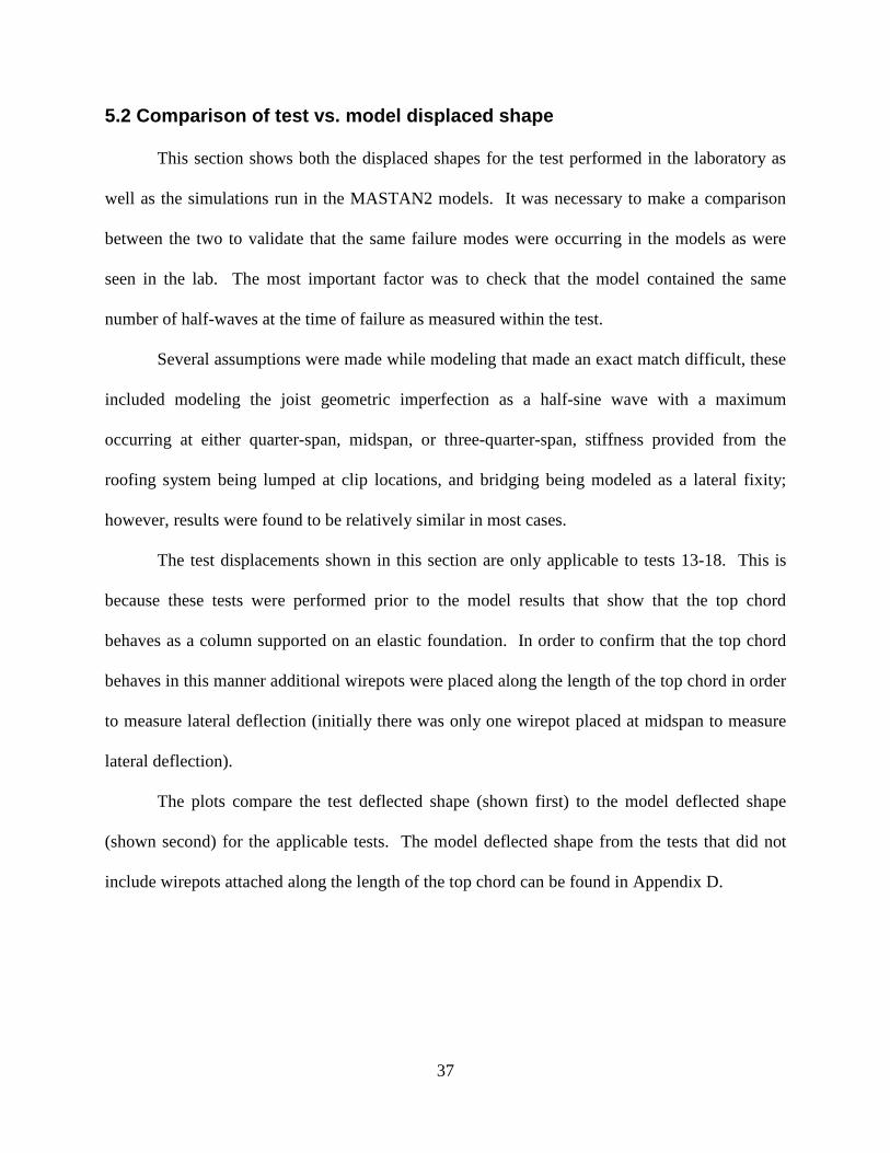
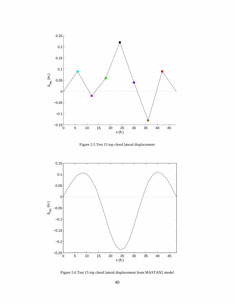
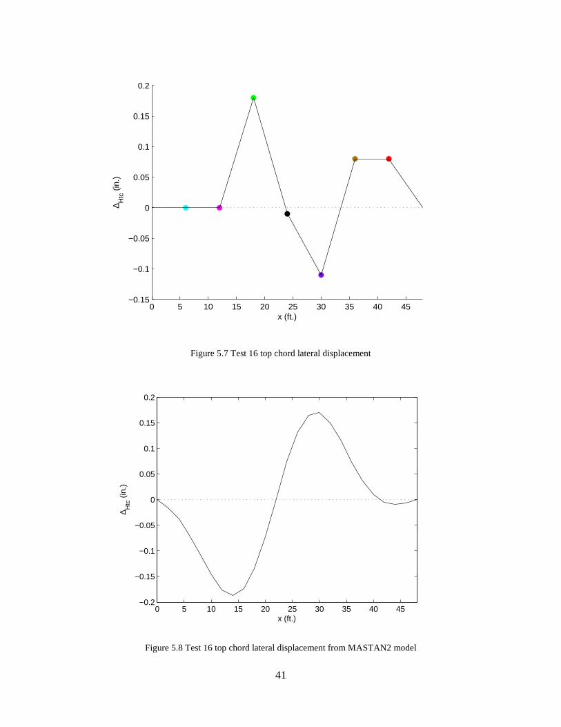
5.2 Comparison of test vs. model displaced shape
This section shows both the displaced shapes for the test performed in the laboratory as
well as the simulations run in the MASTAN2 models. It was necessary to make a comparison
between the two to validate that the same failure modes were occurring in the models as were
seen in the lab. The most important factor was to check that the model contained the same
number of half-waves at the time of failure as measured within the test.
Several assumptions were made while modeling that made an exact match difficult, these
included modeling the joist geometric imperfection as a half-sine wave with a maximum
occurring at either quarter-span, midspan, or three-quarter-span, stiffness provided from the
roofing system being lumped at clip locations, and bridging being modeled as a lateral fixity;
however, results were found to be relatively similar in most cases.
The test displacements shown in this section are only applicable to tests 13-18. This is
because these tests were performed prior to the model results that show that the top chord
behaves as a column supported on an elastic foundation. In order to confirm that the top chord
behaves in this manner additional wirepots were placed along the length of the top chord in order
to measure lateral deflection (initially there was only one wirepot placed at midspan to measure
lateral deflection).
The plots compare the test deflected shape (shown first) to the model deflected shape
(shown second) for the applicable tests. The model deflected shape from the tests that did not
include wirepots attached along the length of the top chord can be found in Appendix D.

38
Figure 5.1 Test 13 top chord lateral displacement
Figure 5.2 Test 13 top chord lateral displacement from MASTAN2 model
0 5 10 15 20 25 30 35 40 45
−1
−0.8
−0.6
−0.4
−0.2
0
0.2
0.4
∆ Htc
(in
.)
x (ft.)
0 5 10 15 20 25 30 35 40 45−0.25
−0.2
−0.15
−0.1
−0.05
0
0.05
0.1
0.15
∆ Htc
(in
.)
x (ft.)

39
Figure 5.3 Test 14 top chord lateral displacement
Figure 5.4 Test 14 top chord lateral displacement from MASTAN2 model
0 5 10 15 20 25 30 35 40 45
−1
−0.8
−0.6
−0.4
−0.2
0
0.2
0.4
∆ Htc
(in
.)
x (ft.)
0 5 10 15 20 25 30 35 40 45−0.4
−0.3
−0.2
−0.1
0
0.1
0.2
0.3
∆ Htc
(in
.)
x (ft.)
40
Figure 5.5 Test 15 top chord lateral displacement
Figure 5.6 Test 15 top chord lateral displacement from MASTAN2 model
0 5 10 15 20 25 30 35 40 45−0.15
−0.1
−0.05
0
0.05
0.1
0.15
0.2
0.25
∆ Htc
(in
.)
x (ft.)
0 5 10 15 20 25 30 35 40 45−0.25
−0.2
−0.15
−0.1
−0.05
0
0.05
0.1
0.15
∆ Htc
(in
.)
x (ft.)
41
Figure 5.7 Test 16 top chord lateral displacement
Figure 5.8 Test 16 top chord lateral displacement from MASTAN2 model
0 5 10 15 20 25 30 35 40 45−0.15
−0.1
−0.05
0
0.05
0.1
0.15
0.2
∆ Htc
(in
.)
x (ft.)
0 5 10 15 20 25 30 35 40 45−0.2
−0.15
−0.1
−0.05
0
0.05
0.1
0.15
0.2
∆ Htc
(in
.)
x (ft.)
42
Figure 5.9 Test 17 top chord lateral displacement
Figure 5.10 Test 17 top chord lateral displacement from MASTAN2 model
0 5 10 15 20 25 30 35 40 45
−1
−0.8
−0.6
−0.4
−0.2
0
0.2
0.4
∆ Htc
(in
.)
x (ft.)
0 5 10 15 20 25 30 35 40 45−0.2
−0.15
−0.1
−0.05
0
0.05
0.1
0.15
∆ Htc
(in
.)
x (ft.)

43
Figure 5.11 Test 18 top chord lateral displacement
Figure 5.12 Test 18 top chord lateral displacement from MASTAN2 model
0 5 10 15 20 25 30 35 40 45−0.2
−0.15
−0.1
−0.05
0
0.05
0.1
0.15
0.2
∆ Htc
(in
.)
x (ft.)
0 5 10 15 20 25 30 35 40 45−0.2
−0.15
−0.1
−0.05
0
0.05
0.1
0.15
∆ Htc
(in
.)
x (ft.)

44
Chapter 6 Conclusions
A new strength prediction approach is presented for open web joists partially braced by a
standing seam roof. The approach employs the AISC (AISI) column curve to calculate top chord
flexural buckling capacity based on the top chord’s critical elastic buckling load. Recently
derived buckling load equations are summarized that account for lateral stiffness provided by the
roof and the parabolically varying axial load from a uniform vertical pressure along the span. A
new hybrid experimental-computational protocol is introduced for approximating standing seam
roof lateral stiffness. The strength prediction approach was verified with a small set of
experiments. Additional experimental verification is needed to fully validate the approach as a
general prediction method for open web joists braced by a standing seam roof.
The strength prediction approach presented in Chapter 2 uses the existing AISC column
curve equations to predict the strength of the top chord by assuming the top chord acts as a
column supported on an elastic foundation. Column slenderness is calculated by using the
equation λc = (Py/Pcre)0.5 where Py is the column yield load and Pcre is the critical elastic buckling
load of the column. The slenderness parameter dictates which column curve equation will be
used (elastic or inelastic buckling). In these equations the only variables needed are those used
in the slenderness equation meaning that the only necessary values to be determined are the yield
load, which is trivial, and the critical elastic buckling load, which is more complex.
To calculate the critical elastic buckling load two methods are given. The first is to
model the top chord appropriately using a structural analysis software program and run an elastic
eigenbuckling analysis; the second is to use the closed form equations given in Chapter 2. It is
necessary to quantify the roof stiffness K (force/length/length) to perform this calculation in
either of the two methods given to calculate the critical elastic buckling load.

45
To determine the stiffness contribution from the roof it is essential to employ a laboratory
testing procedure because the roof stiffness is contingent on the unique properties of each roof
such as clip type, clip height, insulation thickness, presence of a thermal block, joist
imperfection, and the number and location of bridging. A structural analysis computer model of
the joist top chord should then be constructed taking into account the appropriate standing seam
roof properties as discussed in Chapter 3, with the roof stiffness being modeled as either discrete
springs at clip locations or an elastic foundation. The roof stiffness should be iterated until the
second order analysis deflection matches the deflection found in the laboratory experiments.
To validate the data, the results from the laboratory tests should be compared to those
generated from the prediction method. Further validation can be obtained by successfully
modeling the standing seam roof system in a finite element software; Matlab code is available
for writing input files for ABAQUS and is discussed in Appendix F and it is provided in
Appendix G.

46
Chapter 7 Future Work
The research performed at Virginia Tech made it possible to form a prediction method to
determine the capacity of a standing seam roof system. It is necessary; however, for future
studies to be performed on similar roof systems to determine their capacities based on the unique
properties of each roof. This includes altering the joist depth, chord size, span length, clip type,
clip size as well as the roof properties such as insulation thickness and presence of a thermal
block.
There were few tests performed in the Virginia Tech laboratory that included bridging
within the roof system; although the capacities for roof systems with and without bridging were
similar, research that further investigates the behavior of standing seam roof systems including
bridging is suggested.
To better understand the roof behavior a finite element model was created by writing
Matlab code to generate ABAQUS input files. This code includes entering the properties of the
joist, roof, and test to generate a finite element model, this is discussed thoroughly in Appendix
F.

47
References
AISC. (2011). Steel Construction Manual, American Institute of Steel Construction, Fourteenth Edition, United States of America.
Chen, W. F., and Lui, E.M. (1987). Structural Stability Theory and Implementation, Prentice Hall, New
Jersey. Chajes, A. (1974). Principles of Structural Stability, Prentice Hall College Div., Englewood Cliffs, New
Jersey. CSI. (2009). “SAP2000 Advanced 14.0.0.” [Computer software]. Computers and Structures, Inc.
Berkeley, California. <http://www.csiberkeley.com/sap2000> Dassault Systèmes Simulia, (2010). “ABAQUS/CAE 6.10-EF.” [Computer software], Dassault
Systèmes. Providence, RI. <http://www.simulia.com/> Fehr, R. D. (2012), Experiments on Open Web Steel Joists Laterally Braced by a Standing Seam Roof,
Virginia Polytechnic Institute and State University, Blacksburg, Virginia. Fehr, R., Cruishank, S., Moen, C.D. (2012). “Experiments on Open Web Steel Joists Laterally Braced by
a Standing Seam Roof.” Virginia Tech Research Report No. CE/VPI-ST-12/03, Blacksburg, Virginia.
Hodge, P. T. (1986). Lateral Stability of Trusses with Partial Restraint, Master’s Thesis, University of
Minnesota, Minneapolis, Minnesota. Holland, M. V., and Murray, T. M. (1983). Behavior of Steel Joists Supporting Standing Seam Roof
Systems, University of Oklahoma, Norman, Oklahoma. Mathworks. (2010). “Matlab 7.10.0.499 (R2010a).” [Computer software]. Mathworks, Inc.,
<http://www.mathworks.com> Moen, C.D, Cronin, L., Fehr, R. (2012), “Capacity Prediction of Open-Web Steel Joists Partially Braced
by a Standing Seam Roof.” Proc., SSRC. Sherman, D. R., and Fisher, J. M. (1996). "Bracing considerations in standing seam roof systems." Proc.,
SSRC, 493-501. Winter, G. (1958). “Lateral Bracing of Columns and Beams.” Journal of the Structural Division,
Proceedings Paper 1561. Wolfram. (2011). “Wolfram Mathematica 8 For Students” [Computer software]. Wolfram Research, Inc.,
<www.wolfram.com> Ziemian, R. D., and McGuire, W. (2010). “MASTAN2/version 3.3.” [Computer software]. Bucknell
University, Lewisburg, Pennsylvania. <http://www.MASTAN2.com>

48
Appendix A Slenderness proof
This appendix was created to show that the slenderness parameter commonly used in the
AISC code, kL/r, is equivalent to that presented in this paper, (Py/Pcre)0.5. This slenderness
parameter is essential to the prediction method outlined in Chapter 2 because it was difficult to
establish the exact value of k (the effective length factor) for the standing seam roof system.
Rather, it was much simpler to determine the yield load, Py, and the critical elastic buckling load,
Pcre, and relate the top chord capacity to these values.
The proof begins with the AISC column slenderness parameter as defined in Chapter E of
the AISC manual.
yF
E
r
kL71.4≤
( )yF
E
r
kL 2
2
2
71.4≤
By substituting r= (I/A)0.5
( )yF
E
I
AkL 22
71.4≤
yFEI
AkL 171.4
)( 22
≤
yFEI
AkL 171..4)(2
2
2
2
ππ≤
Because Pcre = (π2EI)/(kL)2
ycre FP
A 171.42
2
π≤

49
Multiplying by the right side of the equation by A/A will produce the yield load in the
denominator, and consequently cancel with the A on the left side of the equation.
ycre P
A
P
A2
71.4
π≤
2
271.4
π≤
cre
y
P
P
π71.4≤
cre
y
P
P
π71.4≤
cre
y
P
P
5.1≤cre
y
P
P
50
Appendix B Determination of top chord yield strengt h
Testing procedure
The yield load of the top chord was found through determining the yield stress from
tensile tests, in agreement with ASTM A370-05 “Standard Test Methods and Definitions for
Mechanical Testing of Steel Products”, then multiplying the yield stress by the cross-sectional
area of the top chord. Specimens were taken from each angle within the top chord and tested to
find the yield strength which could then be used in the prediction method.
When joists were received from New Millennium Building Systems they contained
extensions of both the top and bottom chord. Prior to testing the standing seam roof system in
the laboratory the chord extensions were cut to allow for tensile specimens to be formed.
Because the leg of each angle was flat, specimens were cut from the chord extensions in
compliance with ASTM guidelines for the longitudinal flat tension test. The dimensions of the
specimens were in accordance with ASTM 370-05 with a width of 0.5 in. +/- 0.01 in. and were
the full thickness of the section.
Extensions on the top and bottom chord were required while determining the research
plan because the mode of failure was not known at this time. Because nearly all of the tests were
controlled by out-of-plane buckling of the top chord, tension specimens were only taken from the
top chord of each joist.
Prior to testing, the specimens were marked and measured to determine the full stress-
strain relationship of the material as well as the percent elongation and reduction in cross-
sectional area. Gage marks of approximately two inches spaced evenly between the center of the
specimen were made prior to each test with a marker as to not risk cutting into the material thus
creating a stress-concentration. Also measured were the width and thickness of the specimen;

51
calipers were used to measure both of these values and five measurements of each were taken
along the length of the specimen, the average thickness was used while the minimum width was
used, the minimum width was used because it was theorized that it was at the location of
minimum width that the specimen would fracture.
To perform the test an MTS 30-kip capacity tensile machine was used. The data
acquisition system consisted of an extensometer (part of the MTS setup) connected to a computer
which used Testworks4 as the software. The load cell was set to zero before the specimen was
placed in the grips of the tensile machine and was straightened to plumb with the use of a level
before being tightened into place. Once the specimen was in place the extensometer was placed
on the specimen at its approximate center and set to zero using the testing software, Figure B.1
shows the test setup for testing the tensile specimens. The test was then started; the initial rate of
loading was 0.05 in./min. which increased to 0.5 in./min. after yielding occurred.
Figure B.1 Tensile test setup
52
True stress-strain relationship
Testworks4 was able to produce an engineering stress-strain curve as well as the data
points necessary to create this curve; however, it did not produce true stress-strain values which
were necessary to determine the yield strength of the material and for use in plastic analysis
using the finite element model. To transform the engineering stress strain to true stress-strain the
following equations were used:
)1ln( 0εε +=true
)1( 00 εσσ +=true
εtrue and σtrue represent the true stress and strain while ε0 and σ0 represent engineering stress and
strain respectively.
It was necessary for the finite element model to take into account plastic material stress-
strain behavior because it was theorized that some of the chord steel was likely to yield prior to
joist failure during the laboratory experiments. This is where the conversion from engineering
stress-strain to true stress-strain was the most valuable; it can be seen in Figure B.2 that the
linear-elastic region of the stress-strain diagram there is little deviation between the two curves
while the deviation after yielding has occurred is much greater. To produce a model that
accurately described the behavior of the joists as load was applied it was necessary to include
this conversion. The stress-strain curves for the other tests are included at the end of this
appendix.
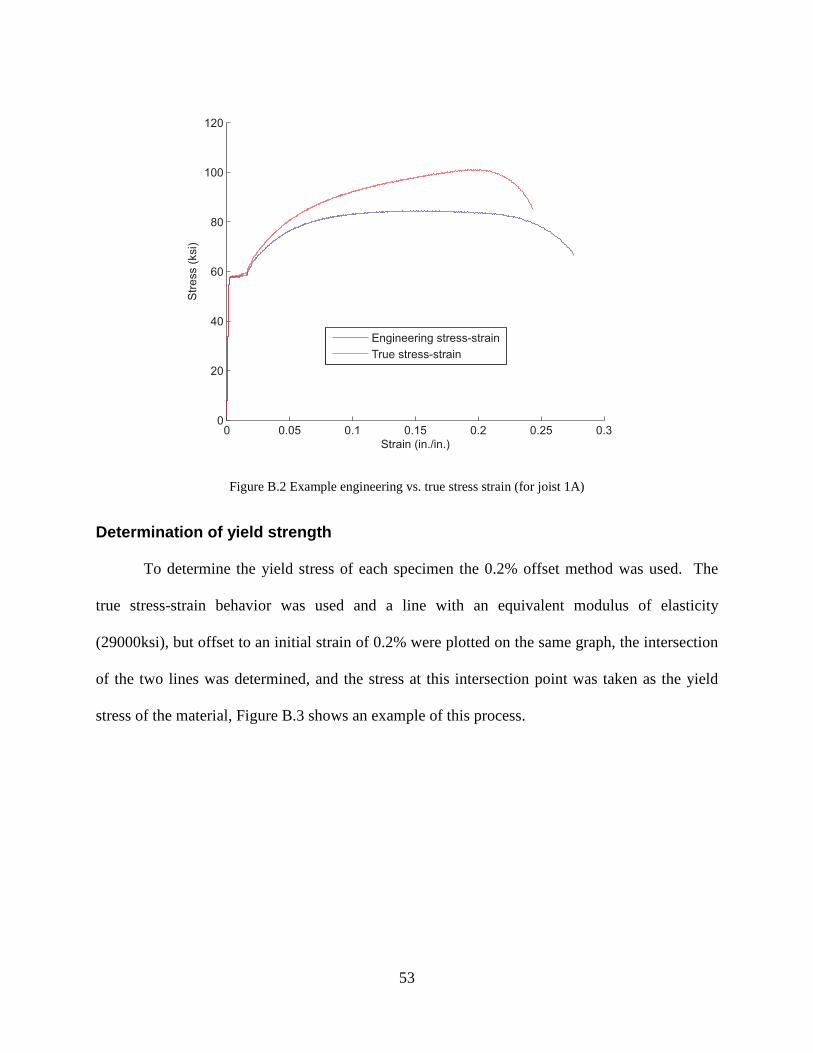
53
Figure B.2 Example engineering vs. true stress strain (for joist 1A)
Determination of yield strength
To determine the yield stress of each specimen the 0.2% offset method was used. The
true stress-strain behavior was used and a line with an equivalent modulus of elasticity
(29000ksi), but offset to an initial strain of 0.2% were plotted on the same graph, the intersection
of the two lines was determined, and the stress at this intersection point was taken as the yield
stress of the material, Figure B.3 shows an example of this process.
0 0.05 0.1 0.15 0.2 0.25 0.30
20
40
60
80
100
120
Strain (in./in.)
Str
ess (
ksi)
Engineering stress-strain
True stress-strain
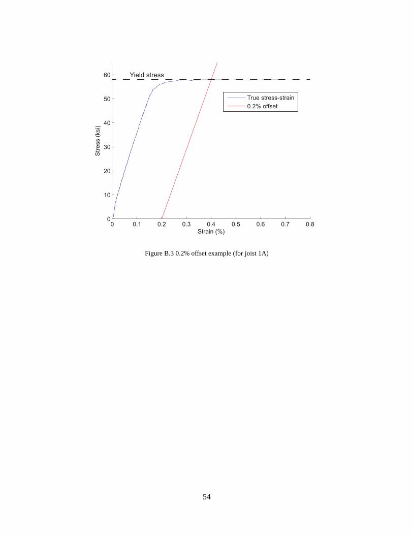
54
Figure B.3 0.2% offset example (for joist 1A)
0 0.1 0.2 0.3 0.4 0.5 0.6 0.7 0.80
10
20
30
40
50
60
Strain (%)
Str
ess (
ksi)
True stress-strain
0.2% offset
Yield stress
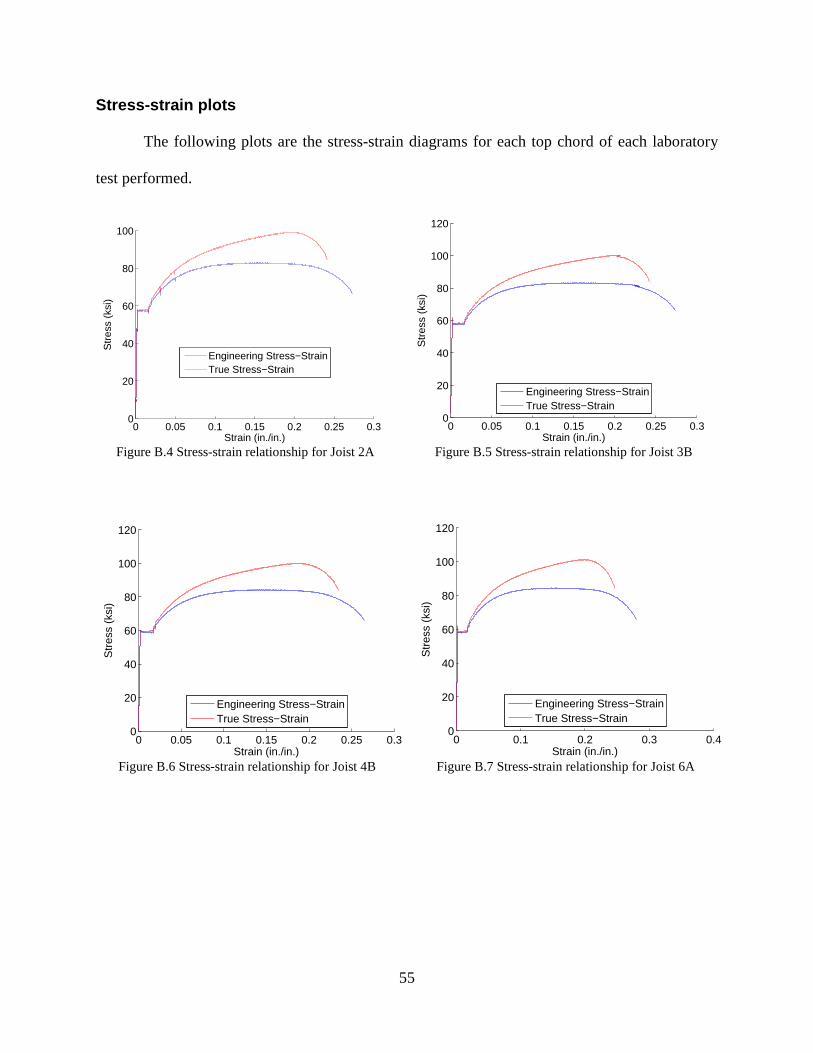
55
Stress-strain plots
The following plots are the stress-strain diagrams for each top chord of each laboratory
test performed.
Figure B.4 Stress-strain relationship for Joist 2A Figure B.5 Stress-strain relationship for Joist 3B
Figure B.6 Stress-strain relationship for Joist 4B Figure B.7 Stress-strain relationship for Joist 6A
0 0.05 0.1 0.15 0.2 0.25 0.30
20
40
60
80
100
Strain (in./in.)
Str
ess
(ksi
)
Engineering Stress−StrainTrue Stress−Strain
0 0.05 0.1 0.15 0.2 0.25 0.30
20
40
60
80
100
120
Strain (in./in.)
Str
ess
(ksi
)
Engineering Stress−StrainTrue Stress−Strain
0 0.05 0.1 0.15 0.2 0.25 0.30
20
40
60
80
100
120
Strain (in./in.)
Str
ess
(ksi
)
Engineering Stress−StrainTrue Stress−Strain
0 0.1 0.2 0.3 0.40
20
40
60
80
100
120
Strain (in./in.)
Str
ess
(ksi
)
Engineering Stress−StrainTrue Stress−Strain
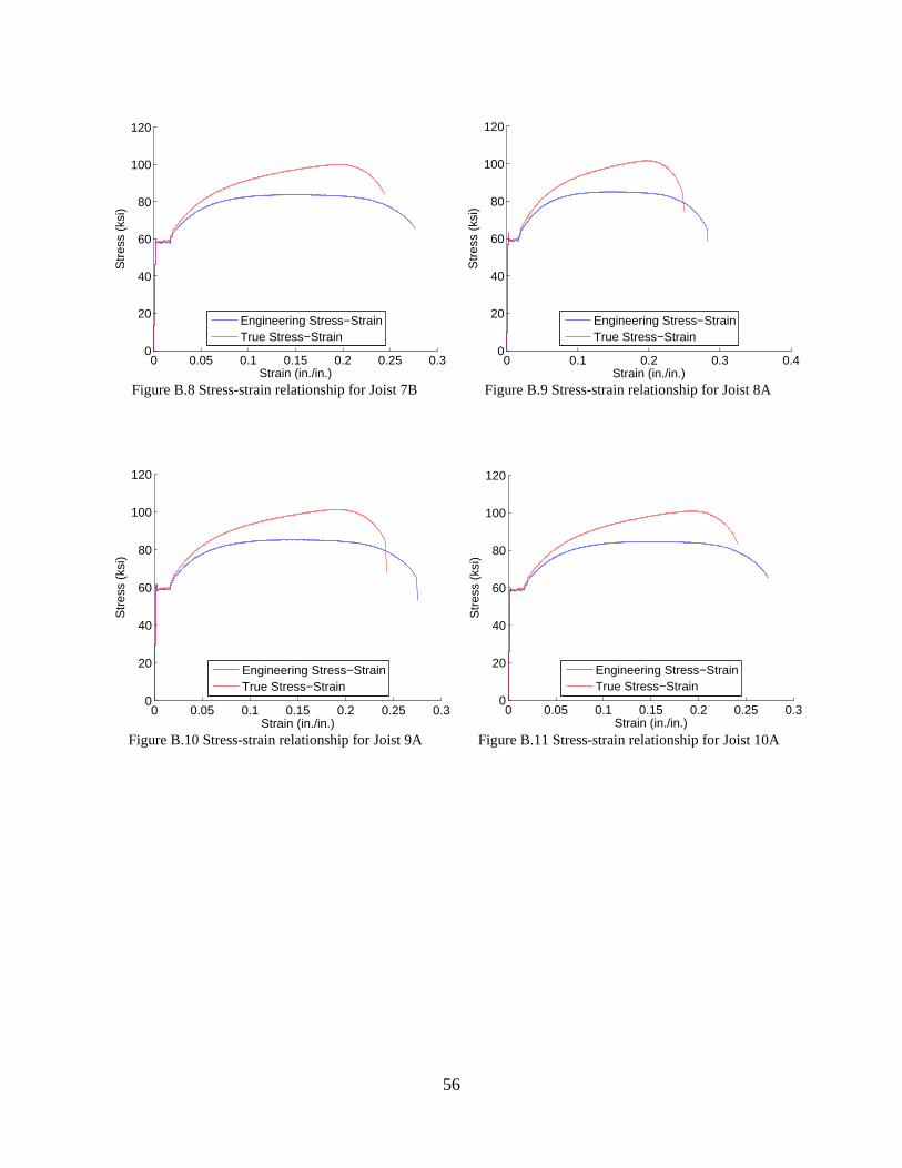
56
Figure B.8 Stress-strain relationship for Joist 7B Figure B.9 Stress-strain relationship for Joist 8A
Figure B.10 Stress-strain relationship for Joist 9A Figure B.11 Stress-strain relationship for Joist 10A
0 0.05 0.1 0.15 0.2 0.25 0.30
20
40
60
80
100
120
Strain (in./in.)
Str
ess
(ksi
)
Engineering Stress−StrainTrue Stress−Strain
0 0.1 0.2 0.3 0.40
20
40
60
80
100
120
Strain (in./in.)
Str
ess
(ksi
)
Engineering Stress−StrainTrue Stress−Strain
0 0.05 0.1 0.15 0.2 0.25 0.30
20
40
60
80
100
120
Strain (in./in.)
Str
ess
(ksi
)
Engineering Stress−StrainTrue Stress−Strain
0 0.05 0.1 0.15 0.2 0.25 0.30
20
40
60
80
100
120
Strain (in./in.)
Str
ess
(ksi
)
Engineering Stress−StrainTrue Stress−Strain

57
Figure B.12 Stress-strain relationship for Joist 11B Figure B.13 Stress-strain relationship for Joist 12A
Figure B.14 Stress-strain relationship for Joist 13B Figure B.15 Stress-strain relationship for Joist 14B
0 0.05 0.1 0.15 0.2 0.25 0.30
20
40
60
80
100
120
Strain (in./in.)
Str
ess
(ksi
)
Engineering Stress−StrainTrue Stress−Strain
0 0.05 0.1 0.15 0.2 0.25 0.30
20
40
60
80
100
120
Strain (in./in.)
Str
ess
(ksi
)
Engineering Stress−StrainTrue Stress−Strain
0 0.05 0.1 0.15 0.2 0.25 0.30
20
40
60
80
100
Strain (in./in.)
Str
ess
(ksi
)
Engineering Stress−StrainTrue Stress−Strain
0 0.05 0.1 0.15 0.2 0.25 0.30
20
40
60
80
100
Strain (in./in.)
Str
ess
(ksi
)
Engineering Stress−StrainTrue Stress−Strain

58
Figure B.16 Stress-strain relationship for Joist 15A Figure B.17 Stress-strain relationship for Joist 16A
Figure B.18 Stress-strain relationship for Joist 18B Figure B.19 Stress-strain relationship for Joist 25B
0 0.05 0.1 0.15 0.2 0.25 0.30
20
40
60
80
100
Strain (in./in.)
Str
ess
(ksi
)
Engineering Stress−StrainTrue Stress−Strain
0 0.05 0.1 0.15 0.2 0.25 0.30
20
40
60
80
100
Strain (in./in.)
Str
ess
(ksi
)
Engineering Stress−StrainTrue Stress−Strain
0 0.05 0.1 0.15 0.2 0.25 0.30
20
40
60
80
100
120
Strain (in./in.)
Str
ess
(ksi
)
Engineering Stress−StrainTrue Stress−Strain
0 0.05 0.1 0.15 0.2 0.25 0.30
20
40
60
80
100
Strain (in./in.)
Str
ess
(ksi
)
Engineering Stress−StrainTrue Stress−Strain

59
Appendix C Measurements
Measurements were taken prior to each laboratory test for analysis purposes as well as to
enter the information into the computer models created. Measurements taken included cross-
sectional measurements, width, height, and thickness of each joist member, web member
location measurements, which included the location of each web member from the end of each
joist, as well as imperfection and camber measurements, in which the initial out of straightness
imperfection was measured; although the model used was simplified and two dimensional, it was
thought that many measurements should be taken for future analysis, such as a finite element
model.
The measurements were used to reach conclusions on effect of different variables, such
as the correlation between imperfection and joist capacity (Fehr 2012; Fehr et al. 2012), as well
as inputs to the structural analysis model, which used the measurements to calculate the moment
of inertia in the lateral direction, cross-sectional area, and nodal coordinates. Furthermore,
measurements taken during testing, such as deflection, and roof load, were used to calculate the
roof stiffness (force/length/length) and loading for the model, see Chapter 4 for more
information.
The cross-sectional measurements taken prior to testing can be seen in Figure C.1. It
should be noted that there was no radius measurements taken for both chord and web members;
however, the radius of the angles in the chord was negligible; while the radius of the web
members was taken as one-half the width.

60
(a)
(b)
Figure C.1 Cross-sectional dimensions of joist members (a) chord dimensions (b) web member dimensions
Additionally initial out-of-straightness measurements were taken prior to each laboratory
test, measurements were taken at quarter-points along each joist to determine the total
imperfection. The imperfection was modeled as a half-sine wave with the model maximum
imperfection location matching both the magnitude and location of that measured prior to testing.
The last measurements taken measured the location of each web member for placement
in the joist; these measurements are valuable for future research if it is desired to model the full
roof system, further discussion of web member placement can be found in Appendix F.
Angle 4 Angle 3
Angle 2 Angle 1
W3
H3
t3
Top Chord
Bottom Chord
H
W
t

61
Appendix D Model displaced shape
The model displaced shapes in Chapter 5 showed that the difference between the actual
behavior of the joists and the behavior as predicted from the MASTAN2 models. Many of the
mode shapes are similar, with a similar number of half-waves in the displaced shape or share the
location of largest displacement with one another.
The following plots show the additional deflected shape from the MASTAN2 second-
order-elastic analysis; as mentioned previously lateral displacement was only measured at
midspan for these tests, so plots that show the test deflected shape are not available.
Figure D.1 Test 1 top chord lateral displacement from MASTAN2 model
0 5 10 15 20 25 30 35 40 45−0.25
−0.2
−0.15
−0.1
−0.05
0
0.05
0.1
∆ Htc
(in
.)
x (ft.)
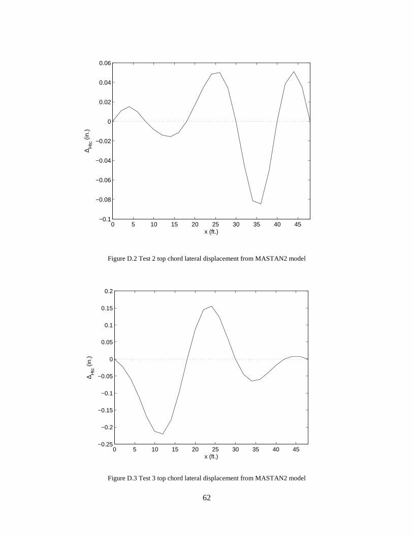
62
Figure D.2 Test 2 top chord lateral displacement from MASTAN2 model
Figure D.3 Test 3 top chord lateral displacement from MASTAN2 model
0 5 10 15 20 25 30 35 40 45−0.1
−0.08
−0.06
−0.04
−0.02
0
0.02
0.04
0.06
∆ Htc
(in
.)
x (ft.)
0 5 10 15 20 25 30 35 40 45−0.25
−0.2
−0.15
−0.1
−0.05
0
0.05
0.1
0.15
0.2
∆ Htc
(in
.)
x (ft.)

63
Figure D.4 Test 4 top chord lateral displacement from MASTAN2 model
Figure D.5 Test 5 top chord lateral displacement from MASTAN2 model
0 5 10 15 20 25 30 35 40 45−0.06
−0.05
−0.04
−0.03
−0.02
−0.01
0
0.01
0.02
0.03
0.04
∆ Htc
(in
.)
x (ft.)
0 5 10 15 20 25 30 35 40 45−0.3
−0.25
−0.2
−0.15
−0.1
−0.05
0
0.05
0.1
0.15
∆ Htc
(in
.)
x (ft.)
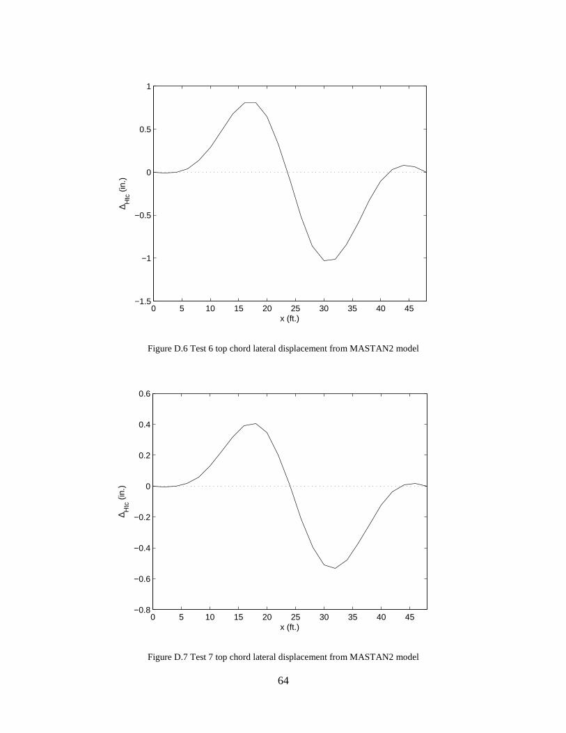
64
Figure D.6 Test 6 top chord lateral displacement from MASTAN2 model
Figure D.7 Test 7 top chord lateral displacement from MASTAN2 model
0 5 10 15 20 25 30 35 40 45−1.5
−1
−0.5
0
0.5
1
∆ Htc
(in
.)
x (ft.)
0 5 10 15 20 25 30 35 40 45−0.8
−0.6
−0.4
−0.2
0
0.2
0.4
0.6
∆ Htc
(in
.)
x (ft.)
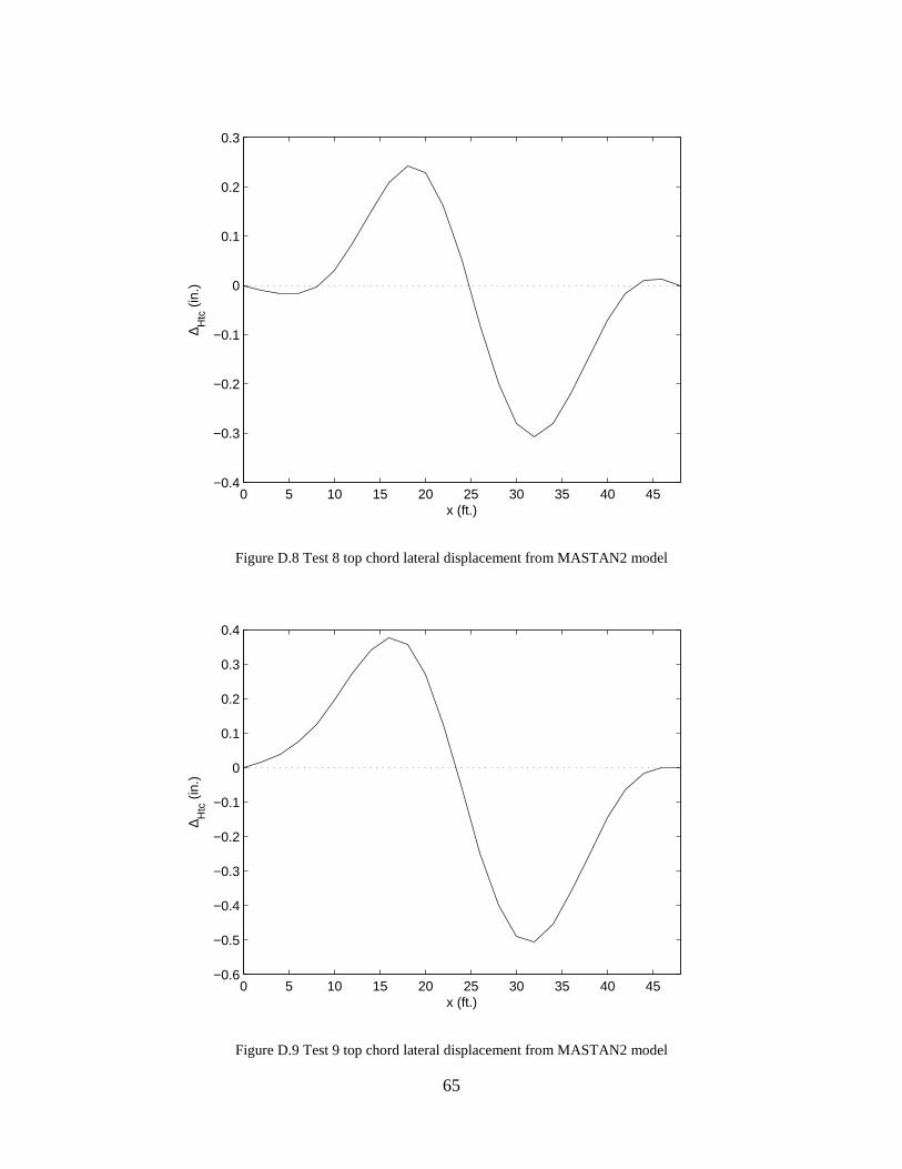
65
Figure D.8 Test 8 top chord lateral displacement from MASTAN2 model
Figure D.9 Test 9 top chord lateral displacement from MASTAN2 model
0 5 10 15 20 25 30 35 40 45−0.4
−0.3
−0.2
−0.1
0
0.1
0.2
0.3
∆ Htc
(in
.)
x (ft.)
0 5 10 15 20 25 30 35 40 45−0.6
−0.5
−0.4
−0.3
−0.2
−0.1
0
0.1
0.2
0.3
0.4
∆ Htc
(in
.)
x (ft.)
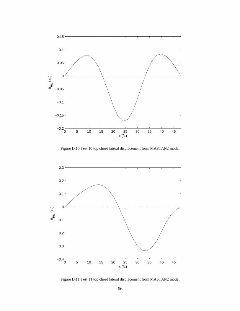
66
Figure D.10 Test 10 top chord lateral displacement from MASTAN2 model
Figure D.11 Test 11 top chord lateral displacement from MASTAN2 model
0 5 10 15 20 25 30 35 40 45−0.2
−0.15
−0.1
−0.05
0
0.05
0.1
0.15
∆ Htc
(in
.)
x (ft.)
0 5 10 15 20 25 30 35 40 45−0.4
−0.3
−0.2
−0.1
0
0.1
0.2
0.3
∆ Htc
(in
.)
x (ft.)

67
Figure D.12 Test 12 top chord lateral displacement from MASTAN2 model
0 5 10 15 20 25 30 35 40 45−0.12
−0.1
−0.08
−0.06
−0.04
−0.02
0
0.02
0.04
0.06∆ H
tc (
in.)
x (ft.)
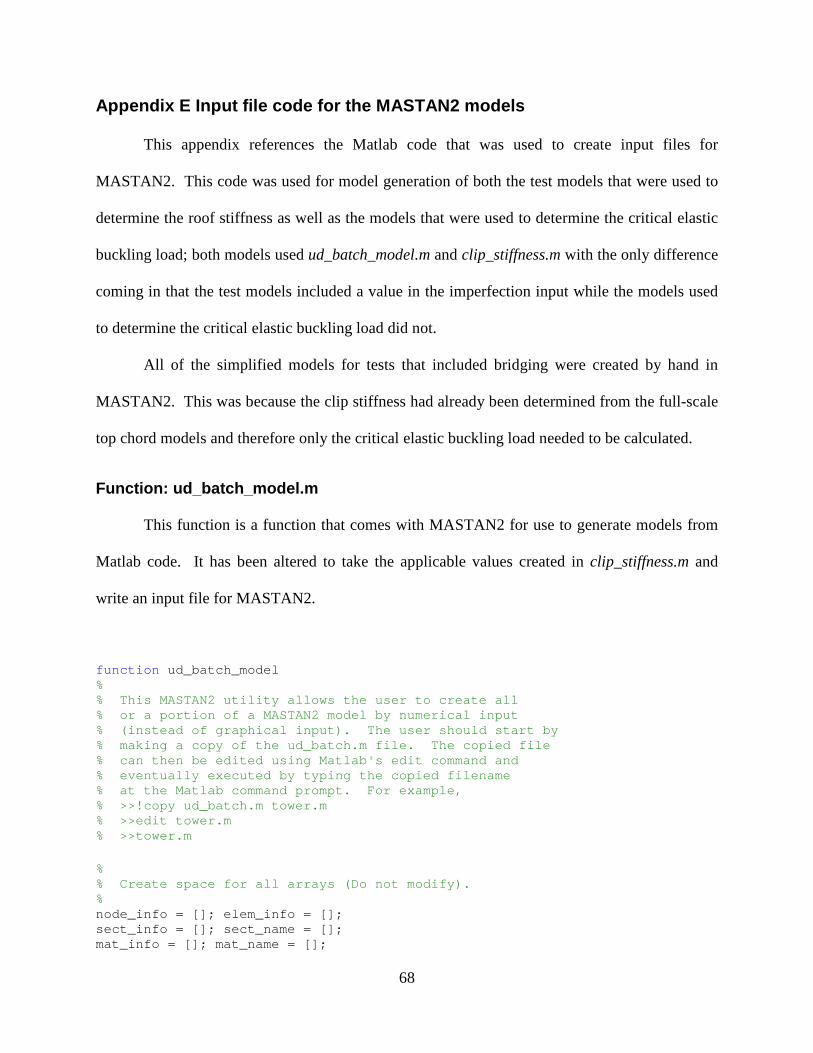
68
Appendix E Input file code for the MASTAN2 models
This appendix references the Matlab code that was used to create input files for
MASTAN2. This code was used for model generation of both the test models that were used to
determine the roof stiffness as well as the models that were used to determine the critical elastic
buckling load; both models used ud_batch_model.m and clip_stiffness.m with the only difference
coming in that the test models included a value in the imperfection input while the models used
to determine the critical elastic buckling load did not.
All of the simplified models for tests that included bridging were created by hand in
MASTAN2. This was because the clip stiffness had already been determined from the full-scale
top chord models and therefore only the critical elastic buckling load needed to be calculated.
Function: ud_batch_model.m
This function is a function that comes with MASTAN2 for use to generate models from
Matlab code. It has been altered to take the applicable values created in clip_stiffness.m and
write an input file for MASTAN2.
function ud_batch_model % % This MASTAN2 utility allows the user to create a ll % or a portion of a MASTAN2 model by numerical inp ut % (instead of graphical input). The user should s tart by % making a copy of the ud_batch.m file. The copie d file % can then be edited using Matlab's edit command a nd % eventually executed by typing the copied filenam e % at the Matlab command prompt. For example, % >>!copy ud_batch.m tower.m % >>edit tower.m % >>tower.m % % Create space for all arrays (Do not modify). % node_info = []; elem_info = []; sect_info = []; sect_name = []; mat_info = []; mat_name = [];
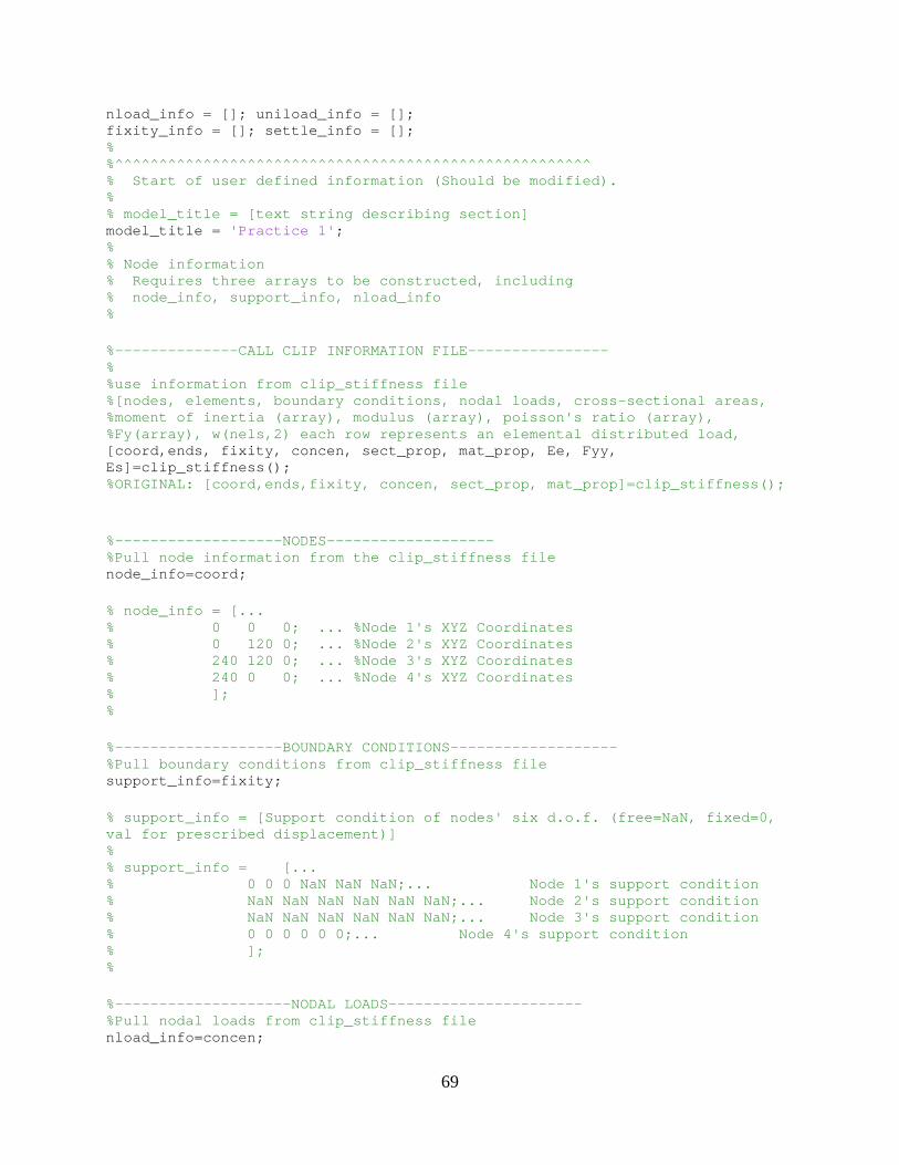
69
nload_info = []; uniload_info = []; fixity_info = []; settle_info = []; % %^^^^^^^^^^^^^^^^^^^^^^^^^^^^^^^^^^^^^^^^^^^^^^^^^^ ^^^^ % Start of user defined information (Should be mod ified). % % model_title = [text string describing section] model_title = 'Practice 1' ; % % Node information % Requires three arrays to be constructed, includi ng % node_info, support_info, nload_info % %--------------CALL CLIP INFORMATION FILE---------- ------ % %use information from clip_stiffness file %[nodes, elements, boundary conditions, nodal loads , cross-sectional areas, %moment of inertia (array), modulus (array), poisso n's ratio (array), %Fy(array), w(nels,2) each row represents an elemen tal distributed load, [coord,ends, fixity, concen, sect_prop, mat_prop, E e, Fyy, Es]=clip_stiffness(); %ORIGINAL: [coord,ends,fixity, concen, sect_prop, m at_prop]=clip_stiffness(); %-------------------NODES------------------- %Pull node information from the clip_stiffness file node_info=coord; % node_info = [... % 0 0 0; ... %Node 1's XYZ Coordinat es % 0 120 0; ... %Node 2's XYZ Coordinat es % 240 120 0; ... %Node 3's XYZ Coordinat es % 240 0 0; ... %Node 4's XYZ Coordinat es % ]; % %-------------------BOUNDARY CONDITIONS------------ ------- %Pull boundary conditions from clip_stiffness file support_info=fixity; % support_info = [Support condition of nodes' six d .o.f. (free=NaN, fixed=0, val for prescribed displacement)] % % support_info = [... % 0 0 0 NaN NaN NaN;... Nod e 1's support condition % NaN NaN NaN NaN NaN NaN;... Nod e 2's support condition % NaN NaN NaN NaN NaN NaN;... Nod e 3's support condition % 0 0 0 0 0 0;... Node 4's su pport condition % ]; % %--------------------NODAL LOADS------------------- --- %Pull nodal loads from clip_stiffness file nload_info=concen;

70
% nload_info = [concentrated force or moment on nod es' six d.o.f.] % % nload_info = [... % 0 0 0 0 0 0;... Node 1's fo rces/moments % 0 -100 0 0 0 0;... Node 2's fo rces/moments % 0 -100 0 0 0 0;... Node 3's fo rces/moments % 0 0 0 0 0 0;... Node 4's fo rces/moments % ]; % %--------------------ELEMENTS-------------------- %Pull element information from clip_stiffness file elem_info=ends; %add in 'inf' into elem info to match up with man-m ade model % Element information % Requires six arrays to be constructed, including % elem_info, uniload_info, thermal_info, sect_info , sect_name, mat_info, mat_name % % % elem_info = [Node i, Node j, Section #, Material #, Beta Angle (rads), ... % Flexure condition Node i (rigid=0,p in=1,spring=2), Flexure condition Node j (rigid=0,pin=1,spring=2), ... % Warping condition Node i (fixed=0,f ree=1,cont=2), Warping condition Node j (fixed=0,free=1,cont=2), ... % Major-axis spring stiffness node i (val = 0 (pin) to inf (rigid)),... % Minor-axis spring stiffness node i (val = 0 (pin) to inf (rigid)),... % Major-axis spring stiffness node j (val = 0 (pin) to inf (rigid)),... % Minor-axis spring stiffness node j (val = 0 (pin) to inf (rigid)),... % Major-axis spring moment capacity M pz node i (val = value to inf (unlimited)),... % Minor-axis spring moment capacity M pz node i (val = value to inf (unlimited)),... % Major-axis spring moment capacity M pz node j (val = value to inf (unlimited)),... % Minor-axis spring moment capacity M pz node j (val = value to inf (unlimited))] % elem_info = [... % 1 2 1 2 0 0 0 0 0 inf inf inf inf inf i nf inf inf;... %Element 1's information % 2 3 2 1 0 0 0 0 0 inf inf inf inf inf i nf inf inf;... %Element 2's information % 4 3 1 2 0 0 0 0 0 inf inf inf inf inf i nf inf inf;... %Element 3's information % ]; %-----------------------UNIFORM LOADS-------------- ------- %Pull distributed load information from clip_stiffn ess file %This input can be the diaphragm force distributed over the length of the

71
%member if we need it, leave it out for now (just m ake it zeros) % uniload_info= uniload_info=zeros(size(elem_info,1),3); % uniload_info = [uniformly distributed loads along elements' local axes (x,y,z)] % % uniload_info = [... % 0 0 0 ;... Element 1's dis tributed load % 0 -.25 0 ;... Element 2's dis tributed load % 0 0 0;... Element 3's dis tributed load % ]; % % %Leave out thermal info, if MASTAN2 gets mad just e nter zeros for %everything thermal_info=zeros(size(elem_info,1),4); % % thermal_info = [thermal effects along elements' l ocal axes, including % thermal coef, dT(centroid), Tgr adient(y'), Tgradient(z')] % % thermal_info = [... % 0 0 0 0;... Element 1's tem p. effects % 0 0 0 0;... Element 2's tem p. effects % 0 0 0 0;... Element 3's tem p. effects % ]; % % Section information % Requires two arrays to be constructed, including % sect_info and sect_name % %---------------------------SECTION INFORMATION---- ------------------------ %Pull in section information from clip_stiffness sect_info=sect_prop; % sizei=size(sect_prop); % difference=12-sizei(1,2); % % for i=difference:1:sizei(1,2) % for j=1:sizei(1,1)%Number of materials % sect_info(j,i)='inf'; % end % end % sect_info = [Area, Moment of inertia Izz, Moment of inertia Iyy, Torsion constant J, % Warping coefficient Cw, Plastic sec tion modulus Zzz, Plastic section modulus Zyy, ... % Shear area Ayy, Shear area Azz YldS urf(1) YldSurf(2) YldSurf(3)] % sect_info = [... % 4.44 48 3.41 0.137 51.8 13.6 2.67 Inf I nf 1 1 1; ... %Section 1's properties
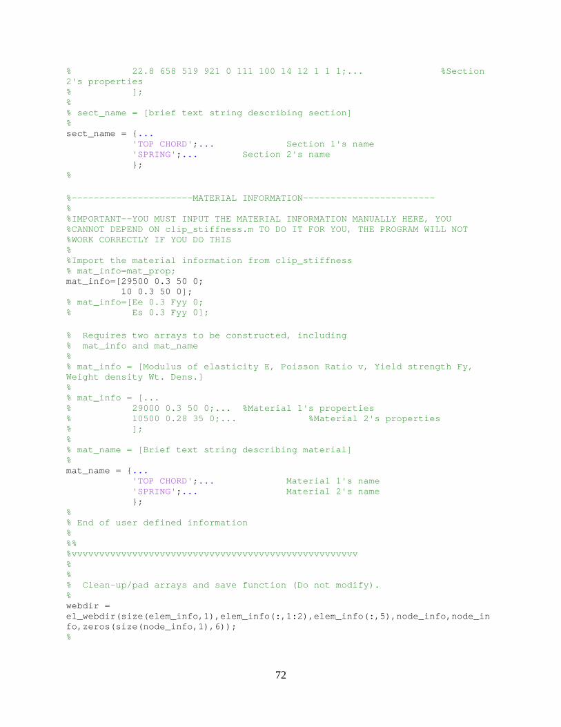
72
% 22.8 658 519 921 0 111 100 14 12 1 1 1; ... %Section 2's properties % ]; % % sect_name = [brief text string describing section ] % sect_name = { ... 'TOP CHORD' ; ... Section 1's name 'SPRING' ; ... Section 2's name }; % %----------------------MATERIAL INFORMATION-------- ---------------- % %IMPORTANT--YOU MUST INPUT THE MATERIAL INFORMATION MANUALLY HERE, YOU %CANNOT DEPEND ON clip_stiffness.m TO DO IT FOR YOU , THE PROGRAM WILL NOT %WORK CORRECTLY IF YOU DO THIS % %Import the material information from clip_stiffnes s % mat_info=mat_prop; mat_info=[29500 0.3 50 0; 10 0.3 50 0]; % mat_info=[Ee 0.3 Fyy 0; % Es 0.3 Fyy 0]; % Requires two arrays to be constructed, including % mat_info and mat_name % % mat_info = [Modulus of elasticity E, Poisson Rati o v, Yield strength Fy, Weight density Wt. Dens.] % % mat_info = [... % 29000 0.3 50 0;... %Material 1's prope rties % 10500 0.28 35 0;... %Materi al 2's properties % ]; % % mat_name = [Brief text string describing material ] % mat_name = { ... 'TOP CHORD' ; ... Material 1's name 'SPRING' ; ... Material 2's name }; % % End of user defined information % %% %vvvvvvvvvvvvvvvvvvvvvvvvvvvvvvvvvvvvvvvvvvvvvvvvvv vv % % % Clean-up/pad arrays and save function (Do not mo dify). % webdir = el_webdir(size(elem_info,1),elem_info(:,1:2),elem_i nfo(:,5),node_info,node_info,zeros(size(node_info,1),6)); %
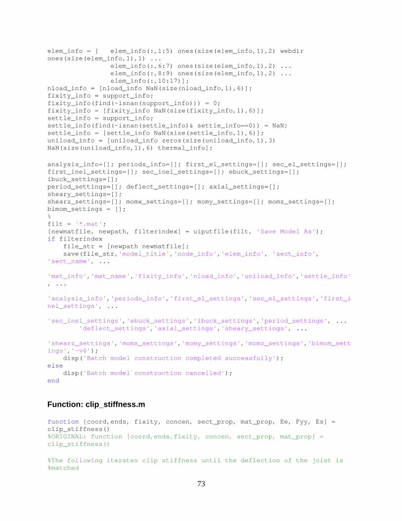
73
elem_info = [ elem_info(:,1:5) ones(size(elem_inf o,1),2) webdir ones(size(elem_info,1),1) ... elem_info(:,6:7) ones(size(elem_inf o,1),2) ... elem_info(:,8:9) ones(size(elem_inf o,1),2) ... elem_info(:,10:17)]; nload_info = [nload_info NaN(size(nload_info,1),6)] ; fixity_info = support_info; fixity_info(find(~isnan(support_info))) = 0; fixity_info = [fixity_info NaN(size(fixity_info,1), 6)]; settle_info = support_info; settle_info(find(~isnan(settle_info)& settle_info== 0)) = NaN; settle_info = [settle_info NaN(size(settle_info,1), 6)]; uniload_info = [uniload_info zeros(size(uniload_inf o,1),3) NaN(size(uniload_info,1),6) thermal_info]; analysis_info=[]; periods_info=[]; first_el_setting s=[]; sec_el_settings=[]; first_inel_settings=[]; sec_inel_settings=[]; ebuck _settings=[]; ibuck_settings=[]; period_settings=[]; deflect_settings=[]; axial_sett ings=[]; sheary_settings=[]; shearz_settings=[]; momx_settings=[]; momy_settings =[]; momz_settings=[]; bimom_settings = []; % filt = '*.mat' ; [newmatfile, newpath, filterindex] = uiputfile(filt , 'Save Model As' ); if filterindex file_str = [newpath newmatfile]; save(file_str, 'model_title' , 'node_info' , 'elem_info' , 'sect_info' , 'sect_name' , ... 'mat_info' , 'mat_name' , 'fixity_info' , 'nload_info' , 'uniload_info' , 'settle_info', ... 'analysis_info' , 'periods_info' , 'first_el_settings' , 'sec_el_settings' , 'first_inel_settings' , ... 'sec_inel_settings' , 'ebuck_settings' , 'ibuck_settings' , 'period_settings' , ... 'deflect_settings' , 'axial_settings' , 'sheary_settings' , ... 'shearz_settings' , 'momx_settings' , 'momy_settings' , 'momz_settings' , 'bimom_settings' , '-v6' ); disp( 'Batch model construction completed successfully' ); else disp( 'Batch model construction cancelled' ); end
Function: clip_stiffness.m
function [coord,ends, fixity, concen, sect_prop, mat_prop, Ee, Fyy, Es] = clip_stiffness() %ORIGINAL: function [coord,ends,fixity, concen, sec t_prop, mat_prop] = clip_stiffness() %The following iterates clip stiffness until the de flection of the joist is %matched

74
% close all % clear all %--------------------INPUTS------------ all units s hould be kips and inches %Test properties W3=1.504; %Height of the cross-section of the chord (in) H3=1.505; %Width of the cross-section of the chord (in) t3=0.149; %Thickness of the top chord (in) W4=1.504; %Height of the cross-section of the chord (in) H4=1.501; %Width of the cross-section of the chord (in) t4=0.13785; %Thickness of the top chord (in) pressure=24.15*1/1000*(1/12)^2; %Pressure on the joists (ksi) delta_max_location=0.5; %Enter the location of the maximum measured displacement in 1/4 points (0.25, 0.5, 0.75) zo=0; %The initial imperfection (sweep) at the center of the joist %default=2.4 s=1.125; %Spacing between the two angles in the top chord (i n) Ee=29500; %The modulus of the top chord (ksi) -- YOU MUST ENT ER THIS UNDER ud_batch_model.m NOT HERE! % Aa=0.3922; %The area of the top chord (in^2) Fyy=50; %The yield strength of the top chord (ksi) % Ii=0.0843; %Moment of inertia of the TC (in^4) yb=(((t3/2)*(W3*t3)+(t3+(H3-t3)/2)*(H3-t3)*t3)+((t4 /2)*(W4*t4)+(t4+(H4-t4)/2)*(H4-t4)*t4))/((W3*t3+(H3-t3)/2*t3)+(W4*t4+(H 4-t4)/2*t4)) %----------OTHER STUFF THAT STAYS PRETTY CONSTANT-- ------- width=5.5*12; %Tributary width of each joist (in.) wpanel=24; %The width of the panel (in.) L=48*12; %Length of the joist (in.) Lb=48*12; %Unbraced length of the joist (dist. between braces ) (in.) LP=2*12; %The spacing of the clips (length of the panel) (sp rings) Lr=16*12; %The distance between the vertical reactions (inche s) d=24; %Depth of the joist (in.) ybar=12; %neutral axis location (from the top of the joist) zm=4; %The maximum deflection of the joist laterally (inc hes) zmax=zm-zo; %The total deflection (movement) of the TC at failu re %Top chord properties cw=0.23272; %Torsional warping constant (from CUFSM output) F1=0.15; %Vertical roller force 1 (kips) F2=0.15; %Vertical roller force 2 (kips) %Assume a linear relationship between the two horiz ontal reactions at %these locations

75
%-------------------SPRING STIFFNESS INFORMATION--- ----------------- %MASTAN does not directly use springs so we need to trick it by inputting %an element and giving it the properties of the spr ing. Since the clips are %acting as vertical springs (they only carry axial load) the MASTAN inputs %that control this are area, modulus of elasiticity , and length. To keep %things simple we will have a constant length (Ls=1 0, this is controlled by %the nodal coordinates), and an equivalent modulus of elasicity (Es=10), %since axial stiffness is AE/L, this should work ou t to have A=clip %stiffness. %New 10/4/2011 -- Change the clip stiffness since w e are getting an %instability in the analysis. Try to use a larger m odulus, smaller area, %and possibly change the length (we can use a lengt h of 1 since all of our %displacements are less than an inch) As=1.0; %Clip stiffness is controlled by AE, make sure that the result of AE/L is equal to the clip stiffness Es=1; %THIS DOES NOT MATTER! YOU MUST ENTER MATERIAL INFORMATION UNDER ud_batch_model.m Lspring=10; %spring length, this should be the same as the spri ng modulus so that stiffness is controlled by the "area" of the s pring %----------------------ANALYSIS INFORMATION-------- ----------- % anatype == flag to indicate which type of analysis is requested % anatype = 1 First-O rder Elastic % anatype = 2 Second- Order Elastic % anatype = 3 First-O rder Inelastic % anatype = 4 Second- Order Inelastic % anatype = 5 Elastic Buckling (Eigenvalue) % anatype = 6 Inelast ic Buckling (Eigenvalue) % anatype=1; %************************************************** ************************ %************************************************** ************************ %Look at the top chord like a column with an imperf ection. Using the spring %stiffness guessed above iterate using the direct s tiffness method until %the deflection converges to the actual measured de flection. % %Assumpions: % * The imperfection and deflected shape occur in a half sine wave % * Model the deflected shape as moments at the l ocation of the clips % % thresh=0.1;%The threshold of how close kclip must be before the loop is terminated %-----Initial basic calculations----- %Calculate the section properties %Moment of inertia %For this calculation the centroid is always in the center of the %two angles that make up the top chord Aa=t3*(W3+(H3-t3))+t4*(W4+(H4-t4)); %Total area (both angles) of the top chord

76
Ii=(1/12*t3*W3^3+(t3*W3)*(s/2+W3/2)^2+1/12* (H3-t3)*(t3^3)+t3*(H3-t3)*(s/2+t3/2)^2)+(1/12*t4*W4^3+(t4*W4)*(s/2+W4/2)^ 2+1/12*(H4-t4)*(t4^3)+t4*(H4-t4)*(s/2+t4/2)^2); %Moment of inertia of the top chord (bending about the z-axis) %Ii=2*(1/12*t*b^3+(t*b)*(s/2+b/2)^2+1/12*(h-t)*(t^3 )+t*(h-t)*(s+t/2)^2); %Moment of inertia of the top chord (bending about the z-axis) r=sqrt(Ii/Aa); %Radius of gyration of the top chord J=1/3*W3*t3^3+1/3*(H3-t3)*t3^3+1/3*W4*t4^3+ 1/3*(H4-t4)*t4^3; %J for the top chord %Unbraced lengths %For the full joist: k=1.0; %Effective length factor (joist end conditions) L=L*k; %Joist effective length %For braced distances: if Lb<L kb=0.5; %Effective length factor of the unbraced length else kb=1; %Effective length factor of the unbraced length (1 if no braces) end Lb=Lb*kb; %Effective unbraced length %Determine the number of clips on the top chord in the unbraced length %region numclips=Lb/LP-1; %The number of clips between braces numclips=round(numclips); %---------------FORCES----------------- %Determine the top chord compressive force P wp=pressure*width; M=wp*L^2/2; P=M/d; %Determine the equivalent distributed load on the p anel (from the panel %reactions (vertical rollers)) Pbrace=(F1+F2)/2; %The average of the brace forces ww=2*Pbrace/L; %Make an array of the displacements at the clip loc ations for j=1:numclips x(j,1)=(j/(numclips+1))*Lb+(L/2-Lb/2); delta(j,1)=zmax*sin(pi*x(j,1)/L); sweep(j,1)=zo*sin(pi*x(j,1)/L); end ticker=2; kclip=0.000001; %clip stiffness (k/in) %************************************************** ************************ %*************************LOOP SHOULD START HERE*** ************************ %************************************************** ************************

77
%---------------------------------NODES------------ ------------------ %Determine node locations in MASTAN %For the beam-element (the TC itself) nnodes=numclips+2; for i=1:nnodes-1 % for i=1:2 coord(i,1)=(i-1)*wpanel; %x-coordinate if delta_max_location==0.25 %if the maximum imperfection is at the 1/4 point of the joist if coord(i,1)<0.25*Lb coord(i,2)=-zo*sin(pi/2*coord(i,1)/(1/4 *Lb)); else coord(i,2)=-zo*(sin(pi/2)*(Lb-coord(i,1 ))/(3/4*Lb)); end elseif delta_max_location==0.75 %if the maximum imperfection is at the 3/4 point of the joist if coord(i,1)<0.75*Lb coord(i,2)=-zo*sin(pi/2*coord(i,1)/(3/4 *Lb)); else coord(i,2)=-zo*sin(pi/2*(Lb-coord(i,1)) /(1/4*Lb)); end else %if the maximum imperfection is at the 1/2 point of the joist coord(i,2)=-zo*sin(pi*coord(i,1)/Lb); %y-coordinate (including imperfection) end end %Put a single node at the center of the structure. This node will be used %as a horizontal reaction (no lateral displacement will occur here) so that %an axial load (P) may be applied (if we pin an end and try to apply an %axial load to that side all of the horizontal load will flow into the pin) new=find(coord(:,1)>=Lb/2); %Determine the nodes that are greater than 1/2 the distance of the unbraced length (we need to add in a node at mid-span) %********UNCOMMENT IF WE NEED CENTRAL NODE****** % save=coord; % for i=1:size(new,1) % coord(new(i,1)+1,:)=save(new(i,1),:); %Move a ll of the coordinates down one spot to make room for the central node % end %Add one more node at the end for the roller next=size(coord,1)+1; coord(next,1)=Lb; %x-coordinate coord(next,2)=0; %y-coordinate %*********CHANGE 10/06 -- TO ACCOUNT FOR SYMMETRY O F NODES % %Make a node at the center of the joist to monito r deflection minnew=min(new); %Determine the lowest value in new to know where th e central node is supposed to go % %'new' is an array of nodes with an x-coordinate greater
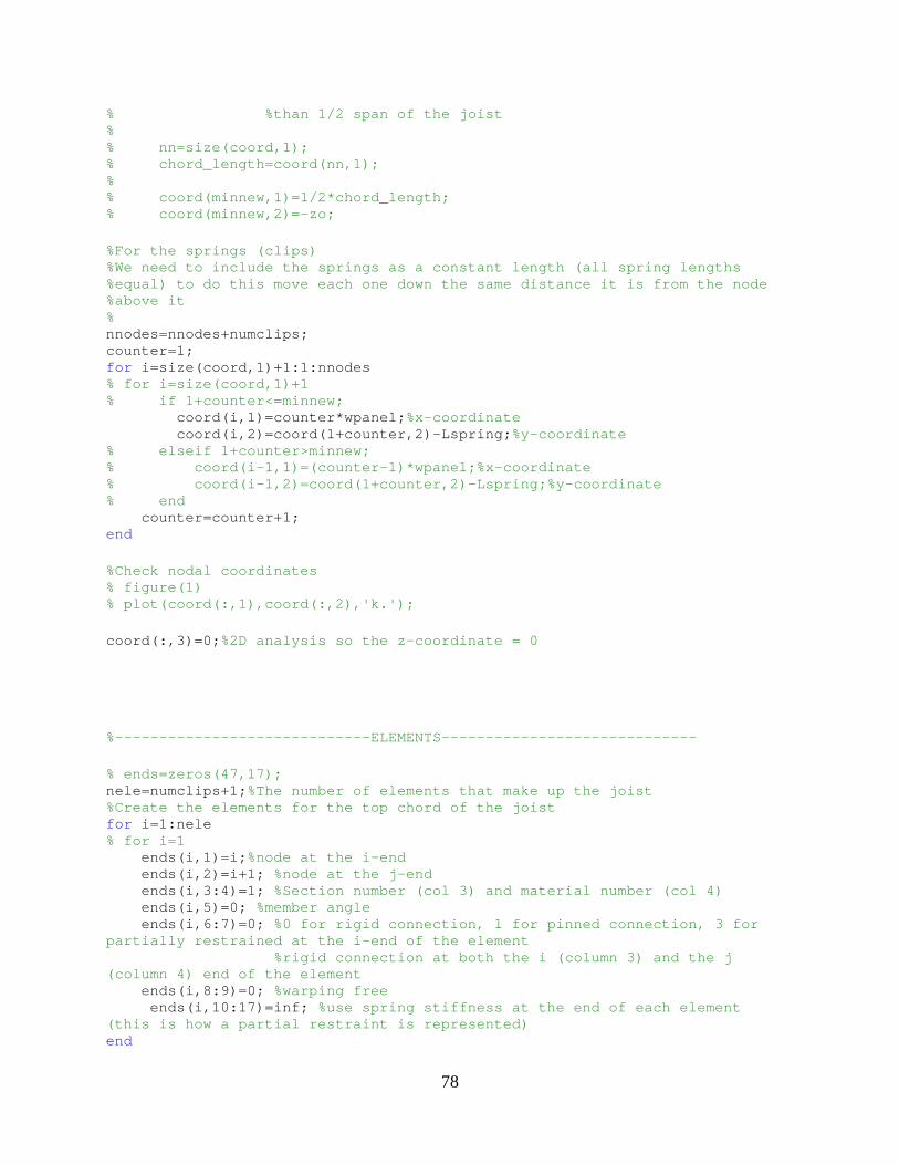
78
% %than 1/2 span of the joist % % nn=size(coord,1); % chord_length=coord(nn,1); % % coord(minnew,1)=1/2*chord_length; % coord(minnew,2)=-zo; %For the springs (clips) %We need to include the springs as a constant lengt h (all spring lengths %equal) to do this move each one down the same dist ance it is from the node %above it % nnodes=nnodes+numclips; counter=1; for i=size(coord,1)+1:1:nnodes % for i=size(coord,1)+1 % if 1+counter<=minnew; coord(i,1)=counter*wpanel; %x-coordinate coord(i,2)=coord(1+counter,2)-Lspring; %y-coordinate % elseif 1+counter>minnew; % coord(i-1,1)=(counter-1)*wpanel;%x-coordi nate % coord(i-1,2)=coord(1+counter,2)-Lspring;% y-coordinate % end counter=counter+1; end %Check nodal coordinates % figure(1) % plot(coord(:,1),coord(:,2),'k.'); coord(:,3)=0; %2D analysis so the z-coordinate = 0 %-----------------------------ELEMENTS------------- ---------------- % ends=zeros(47,17); nele=numclips+1; %The number of elements that make up the joist %Create the elements for the top chord of the joist for i=1:nele % for i=1 ends(i,1)=i; %node at the i-end ends(i,2)=i+1; %node at the j-end ends(i,3:4)=1; %Section number (col 3) and material number (col 4) ends(i,5)=0; %member angle ends(i,6:7)=0; %0 for rigid connection, 1 for pinned connection, 3 for partially restrained at the i-end of the element %rigid connection at both the i (column 3) and the j (column 4) end of the element ends(i,8:9)=0; %warping free ends(i,10:17)=inf; %use spring stiffness at the end of each element (this is how a partial restraint is represented) end
79
%Change the elements so that the node in the center of the top chord is %included in the element list %Create elements for the springs %change this to look like it does above (using the same columns) nele=nele+numclips; %number of elements including the springs nodemax=numclips+4; counter=2; %Start with counter=2 b/c this is the first node th at uses a spring for i=size(ends,1)+1:1:nele % for i=size(ends,1)+1 % if counter<minnew ends(i,1)=nodemax+counter-3; ends(i,2)=counter; %We want to use a pin in each spring where it conne cts to the top %chord, this is to not allow the spring to hold mom ent (it is %strictly an axial member) ends(i,3:4)=2; %Section number (col 3) and material number (col 4) ends(i,5)=0; %member angle ends(i,6)=0; %0 for rigid connection, 1 for pinned connection, 3 for partially restrained at the i-end of the element %We want a rigid connection at the base (i end) of each spring element ends(i,7)=0; %We want a rigid connection at the top (j end) of e ach spring element ends(i,8:9)=0; %warping free ends(i,10:17)=inf; %use spring stiffness at the end of each element (this is how a partial restraint is represented) % elseif counter>=minnew % next=size(ends,1); % ends(next+1,1)=nodemax+counter-2;%The spr ing node stays the same % ends(next+1,2)=counter;%We need to skip o ver the middle node since it does not have a spring attached to it % ends(next+1,3:4)=2;%Section number (col 3 ) and material number (col 4) % ends(next+1,5)=0;%member angle % ends(next+1,6)=0;%0 for rigid connection, 1 for pinned connection, 3 for partially restrained at the i-end of the elem ent % %We want a rigid connection a t the base (i end) of each spring element % ends(next+1,7)=0;%We want a pinned connec tion at the top (j end) of each spring element % ends(next+1,8:9)=0; %warping free % ends(next+1,10:17)=inf; %use spring stif fness at the end of each element (this is how a partial restraint is represe nted) % end counter=counter+1; end %--------------------------BOUNDARY CONDITIONS----- ------------------------

80
%Apply boundary conditions to the appropriate nodes %CHANGE 10/7 -- ORIGINAL: fixity=NaN(size(coord,1), 6) fixity=NaN(size(coord,1),6); for i=1:size(coord,1); if i==1 % fixity(i,1)=0;%fixes the x-displacement o f the first node (pin) fixity(i,2)=0; %fixes the y-displacement of the first node (pin) % fixity(i,3)=0;%fixes the z-displacement o f the first node % (unnecessary) elseif i==numclips+2 % elseif i==2 fixity(i,2)=0; %fixes the y-displacement of the first node (pin) elseif i==minnew %Fix the x-dirctional displacement at the mid-span node fixity(i,1)=0; %Fixes the x-displacement at mid-span elseif i>numclips+2 %Let's try to only have the springs be fixed in the y-direction %(rollers) % fixity(i,1)=0;%fixes the x-displacement o f the spring nodes (pin) fixity(i,2)=0; %fixes the y-displacement of the spring nodes (pin) end end %---------------------CONCENTRATED LOADS----------- ------------ %Apply concentrated moments at node locations %These moments are due to second order effects--The y ONLY take into account %the moments before failure! (don't include the inc rease in deflection as %the load is increased) %CHANGE!!!! 9/16 -- We can just run a second order- analysis. We do NOT need %to include these moments; however, the axial force increases as we move %towards the center of the joist. Therefore we need to increase the load at %each clip location %Make an array of zeros and replace the zeros with the applied loads concen=zeros(size(coord,1),6); xloc(1)=(L/2-Lb/2); %Beginning of the brace location xloc(2)=(L/2+Lb/2); %End of the brace location pmax=wp*(L/2)^2/(2*d); %Write code for an axial force that increases as we move towards the center %of the top chord % counter=1; for i=1:numclips+2 % for i=1:2 xcoord=coord(i,1); %The x-location of the node with the load being app lied to it concen(i,1)=(4*pmax*xcoord)/(L)*(1-xcoord/L ); %axial load for those nodes on the first 1/2 of the joist counter=counter+1;

81
end % counter=1; % for i=1:numclips+2 % % for i=1:2 % xcoord=coord(i,1);%The x-location of the node with the load being applied to it % if counter < numclips/2+2 % concen(i,1)=(wp*xcoord^2)/(2*d);%axial lo ad for those nodes on the first 1/2 of the joist % elseif i>minnew % concen(i,1)=-(wp*(Lb-xcoord)^2)/(2*d);%ax ial load for those nodes on the second 1/2 of the joist % end % counter=counter+1; % end % figure(1) % plot(coord(:,1),concen(:,1)) %apply loads so that the TOTAL axial load increases parabolically towards %the center save=concen; %save the loads in concen before altering them to a pply the actual loads new_concen=zeros(size(coord,1),6); for i=1:numclips+2; if i==1 new_concen(i,1)=concen(i,1); elseif i==size(concen,1) new_concen(i,1)=concen(i,1); else new_concen(i,1)=concen(i,1)-save(i-1,1); end end concen=new_concen; %change concen to the new loads % figure(2) % plot(coord(:,1),concen(:,1),'.k') %Make a plot to show how the axial force is varying over the TC length % Pmax=(wp*(Lb/2)^2)/(2*d);%The maximum axial force in the top chord % xx=0:0.1:L; %The x-length runs from 0-48ft % yy=Pmax*(sin(pi*xx/(L))); % figure(1) % plot(xx,yy) % title('Top Chord Axial Load Variation') % xlabel('Top Chord Length (ft.)') % ylabel('Axial load (kips)') % counter=1; % for i=1:numclips+2 % if i==1 % concen(i,3)=-P*zo*sin(pi*xloc(1)/L);

82
% elseif i==numclips+2 % concen(i,3)=P*zo*sin(pi*xloc(2)/L); % else % if counter<numclips/2 % concen(i,3)=-P*sweep(counter,1);%mome nts for the springs on the first 1/2 of the joist % counter=counter+1; % else % concen(i,3)=P*sweep(counter,1);%momen ts for the springs on the second 1/2 of the joist % counter=counter+1; % end % end % end %--------------------------SECTIONS AND MATERIALS-- --------------------- %Define both sections as well as materials on an el ement-to-element basis %the top chord members always are defined first and then the spring (clip) %members are defined %Make section properties an array of zeros and then fill it in with the %appropriate values % sect_prop=NaN(2,12); % sect_prop=zeros(2,5); %Define the section properties in terms of the numb er of sections (2) that %we are using (we have two sections because we have two members (top chord %and springs) that we are using) sect_prop(1,1)=Aa; %Area of the top chord as defined in the input sect_prop(1,2)=Ii; %The moment of inertia as defined in the input sect_prop(1,3)=Ii; %Iyy (doen't matter for 2D beam) sect_prop(1,4)=J; %Torsion constant J for the top chord sect_prop(1,5)=cw; %Torsional warping constant (from CUFSM output) sect_prop(1,6:7)=Inf; %Plastic section modulus (Zzz, and Zyy respectively ) sect_prop(1,8:9)=Inf; %Shear area for the z and y axes respectively sect_prop(1,10:12)=1; %Shear area? % sect_prop(1,4:9)=5;%A bunch of things that do n't apply to a 2D analysis %now the springs sect_prop(2,1)=As; %The clip stiffness is controlled by this parameter IMPORTANT!!! sect_prop(2,2)=0.9999; %The moment of inertia does not matter for the clips, stiffness is controlled by AE/L sect_prop(2,3)=1; %Iyy (doen't matter for 2D beam) sect_prop(2,4:5)=0; %Torsional coefficients J and Cw respectively sect_prop(2,6:9)=Inf; %A bunch of things that don't apply to a 2D analysi s sect_prop(2,10:12)=1; %Shear area? mat_prop=[Ee 0.3 Fyy 1; Es 0.3 Fyy 1]; % mat_prop(1,1)=Ee;%Top chord modulus of elasti city % mat_prop(1,2)=0.3;%Poisson's ratio of steel
83
% mat_prop(1,3)=Fyy;%Yield strength % mat_prop(1,4)=1;%Weight density (it is not ac ting down so neglect this) % %now the springs % mat_prop(2,1)=Es;%Use the 'modulus' of the sp ring as defined in the input, this should be the same as the length of eac h spring to allow for the spring stiffness to be controlled by the area of th e spring % mat_prop(2,2)=0.3;%Poisson's ratio % mat_prop(2,3)=Fyy;%Yield strength % mat_prop(2,4)=1;%Weight density (it is not ac ting down so neglect this) % %Define the spring members % for i=numclips+2:1:nele % A(i)=As;%The clip stiffness is controlled by this parameter IMPORTANT!!! % Izz(i)=1; %The moment of inertia does not mat ter for the clips, stiffness is controlled by AE/L % E(i)=Es; %Use the 'modulus' of the spring as defined in the input, this should be the same as the length of each spring to allow for the spring stiffness to be controlled by the area of the sprin g % v(i)=0.3; % Fy(i)=Fyy; % w(i,1:2)=0; %no distributed load on the sprin gs % end %Define the top chord members % for i=1:numclips+1 % A(i)=Aa; %Area of the top chord as defined in the input % Izz(i)=Ii; %The moment of inertia as defined in the input % % Zzz(i)=1; %use 1 as default, enter if known % % Ayy(i)=1; %use 1 as default, enter if known % E(i)=Ee; %Young's modulus as defined in the i nput % v(i)=0.3; %Poisson's ratio of steel, change f or other materials % Fy(i)=Fyy; %The yield strength as defined in the input % % % YldSurf(i)=1;%element i's yield surface max imum values % % YldSurf(i,1) = max imum P/Py value % % YldSurf(i,2) = max imum Mz/Mpz value % % YldSurf(i,3) = max imum My/Mpy value % % Wt(i)=1; %weight density % % webdir(i,1:3) == element i's unit web v ector. This is a unit vector % % that defines the eleme nt's local y-y axis with respect % % to the global coordina te system. It is based only on the % % structures undeformed geometry. % % webdir(i,1) = x comp onent of element's unit web vector % % webdir(i,2) = y comp onent of element's unit web vector % % webdir(i,3) = z comp onent of element's unit web vector % % (which will always be zero for 2D analysis)

84
% % NOTE: An element's 3x3 rotation matrix, [g], is constructed % % as follows: First, cal culate a unit vector, x_vect, that % % describes the element' s local x-axis (be sure to include % % all three components w ith the z component always being zero). % % Second, take the cross product of x_vect and webdir(i,:) to % % obtain z_vect, i.e. z_ vect = cross(x_vect,webdir(i,:)). Third, % % set z_vect to a unit v ector, i.e. z_vect = z_vect/norm(z_vect). % % For 2D analysis, z_vec t will be either [0 0 1] or [0 0 -1]. % % Finally, the first row of [g] is x_vect, its second row is % % webdir(i,:), and its t hird row is z_vect. % % w(i,2)=-ww; %Element i's uniform load in the y-direction, negative is for a downward load % w(i,1)=0;%There is no load in the x=-directio n % end % %Define the spring members % for i=numclips+2:1:nele % A(i)=As;%The clip stiffness is controlled by this parameter IMPORTANT!!! % Izz(i)=1; %The moment of inertia does not mat ter for the clips, stiffness is controlled by AE/L % E(i)=Es; %Use the 'modulus' of the spring as defined in the input, this should be the same as the length of each spring to allow for the spring stiffness to be controlled by the area of the sprin g % v(i)=0.3; % Fy(i)=Fyy; % w(i,1:2)=0; %no distributed load on the sprin gs % end truss=0; %Flag to let MASTAN know that the system is NOT a t russ %************************************************** ************************ %************************************************** ************************

85
Appendix F Finite element model generation
It was desired to use a finite element model to analyze the standing seam roof systems to
better understand their behavior as they were loaded. The finite element software used for this
process was ABAQUS with input files being written from Matlab. Models were generated by
supplying Matlab with measurements taken prior to testing, member cross-sectional properties,
imperfection measurements, etc., as well as other applicable information, such as failure load,
roof stiffness, etc. Analysis consisted of simulating the test using a collapse model which uses a
load deflection analysis (reffered to as a Riks analysis). In this analysis both the load and the
deflection are iterated in steps along the static equilibrium path until the solution is stable, then
the next step is taken and the process continues until the model fails.
As research progressed it was determined that simplified models could be created and
analyzed and that finite element models were not essential; although they would have been
helpful. It was found that time spent on establishing and critiquing the prediction method was
more beneficial than modifying the finite element models to share the same results as those
found in the laboratory.
Because analysis finite element models were not used in establishing the prediction
method, this section references the Matlab code and how the code is to be used to generate finite
element models in ABAQUS. The goal of this section is to allow any future work performed on
this subject to be able to utilize the Matlab input file code to easily create their own finite
element models.
The Matlab code was created so that it could be used for different roofing systems by
changing only a few inputs. Files are included for single joist models, multiple joist models, and
top chord models, all models include default settings to include boundary conditions, constraints
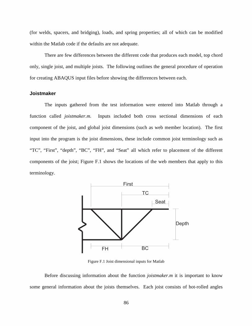
86
(for welds, spacers, and bridging), loads, and spring properties; all of which can be modified
within the Matlab code if the defaults are not adequate.
There are few differences between the different code that produces each model, top chord
only, single joist, and multiple joists. The following outlines the general procedure of operation
for creating ABAQUS input files before showing the differences between each.
Joistmaker
The inputs gathered from the test information were entered into Matlab through a
function called joistmaker.m. Inputs included both cross sectional dimensions of each
component of the joist, and global joist dimensions (such as web member location). The first
input into the program is the joist dimensions, these include common joist terminology such as
“TC”, “First”, “depth”, “BC”, “FH”, and “Seat” all which refer to placement of the different
components of the joist; Figure F.1 shows the locations of the web members that apply to this
terminology.
Figure F.1 Joist dimensional inputs for Matlab
Before discussing information about the function joistmaker.m it is important to know
some general information about the joists themselves. Each joist consists of hot-rolled angles
Seat
TC
First
BCFH
Depth

87
that make up each chord, and cold-formed steel web members. An easy way to think of the web
members is in sets of three, as can be seen in Figure F.2.
Figure F.2 Elevation of a typical joist showing web member “groups”
The orientation and placement of the first set of web members (on either side of the joist)
depends on the initial inputs first, TC, seat, FH, and BC, while all other web members are placed
based on the additional spacing between web members and overall joist length. All sets of web
members other than the first set consist of two web members angled at 45 degrees above the
horizontal in either direction, and one vertical member.
The inputs for the joist dimensions are input as vectors, this input was chosen to allow for
multiple joist dimensions to be input into the same file so that if multiple joists are desired the
program will be able to take the dimensions of each joist into account separately.
Other inputs into the program include the length of the top chord, the number of joists,
the center-to-center spacing of the joists, the center-to-center spacing of the web members (the
location where they come together in the top and bottom chords), the depth at which the web
members sit below the extreme fiber of each chord, the number of brace points in each joist, the
value of the maximum imperfection (assumed to be a half-sine wave), the loading condition
(either point loads at the clip locations or a uniform pressure load across the top chord), and clip
spacing. Many of the inputs are described in more detail later in this section.
Group of 3 web members

88
The last input into the program is the cross-sectional information of each of the
components of the joist. This includes the thickness, height, and width of each member; inputs
are selected based on the values measured prior to each laboratory test, Figure F.3 shows these
measurements. It should be noted that the web member length is never input into the program;
rather joistmaker.m calculates the length of each web-member based on the web-member inputs
(First, TC, etc.) as well as the length of the joist. It should be noted that the cross-sectional
inputs are not in the very beginning of the joistmaker.m function but rather later in the function
closer to where each component is generated.
Figure F.3 Cross-sectional dimensions of joist members (a) chord dimensions (b) web member dimensions
The first step in creating the model is to place nodes around the cross-section.
joistmaker.m uses S9R5 elements as a default and thus the number of elements within each
cross-section must be an even number to allow a whole number of elements to be formed
(corresponding to an odd number of nodes). This is because the S9R5 elements use 3 nodes per
side of each element; when the program creates elements within the cross-section it links
adjacent nodes together thinking that two nodes are an “element”; however, because it takes 3
Angle 4 Angle 3
Angle 2 Angle 1
W3
H3
t3
Top Chord
Bottom Chord
H
W
t

89
nodes to form an S9R5 element this is the equivalent of two cross-sectional “elements”. The
number of elements within each cross-section is controlled by the variable n which is a matrix
that contains the number of elements that are present on each component of each member. For
example, an angle in the top chord of a joist has three distinct parts, two legs and a fillet, the
required inputs into n for this member are n = [4, 4, 4] for each of these sections (if four elements
are required for each section), Figure F.4 shows an example of how n is translated into the cross-
section.
Figure F.4 Number of cross-sectional elements for a typical top chord angle
The previously mentioned inputs work with the cross-sectional information to form each
cross-section. The cross-sections are formed by placing nodes evenly across each section of
each member (for example Section 1, 2, or 3 of Figure F.4) and then placing elements between
the appropriate nodes, this step is completed with a variety of functions (webxy.m, TCxy3.m,
BCxy1.m, etc.) the exact function found for each component can be found in
Table F.1.
The next step is for the program to take the cross-sectional inputs and member lengths
and extrude each joist component to its full length. It is extruded through a function called
x_sect_to_abaqus.m which places nodes along the length of the member until the member length
is met. Additionally it creates elements between the applicable nodes; this function is used
n = [4, 4, 4]
Section 1 = 4 elementsSection 2 = 4 elements
Section 3 = 4 elements

90
multiple times, once for every time joistmaker.m creates a different member of the joist (and thus
is found in multiple places in joistmaker.m).
After each member is created it is placed into the global coordinate system through an
assembly function that is unique for each member type (there is a different assembly function for
web members and chord members); Table F.1 shows the different assembly functions and their
corresponding members. These functions take each member within its local coordinates and
make the appropriate nodal transformations for each member to be placed in the global
coordinate system.
The functions TCassem3.m, TCassem4.m, BCassem1.m, and BCassem2.m have another
purpose, to create constraints, boundary conditions, loads, and springs (to model the clips) for the
finite element model. Constraints are needed for welds, brace points, and spacers to simulate
joist behavior during testing. Welds were modeled as multi-point-constraints (MPC) in which
nodes are tied to one another sharing a certain number of degrees of freedom. To model the
welds between the web members and the chord angles the assembly functions would search
through the nodes of each angle of each chord and determine the node numbers within each
chord angle that most-closely corresponded to those at the end of each web member and then tie
them together with a MPC.
Similarly, for spacers (which are used as an intermediate connector for each chord
between web members) are modeled as a MPC with each node within a leg of each chord being
constrained with a MPC. It should be noted that there is a section within joistmaker.m that is
used for the creation of spacers; this section is not used for creating physical spacers; however, it
is used to determine the location of each spacer. It is also important to mention that spacer
location is dependent on the joist design, which is dictated by the manufacturer, joistmaker.m is

91
designed to place spacers in compliance with 48 ft. span 24K4 joists as designed by New
Millennium Building Systems for the pressure box tests at Virginia Tech, which is unlikely to
match up with other designs.
Bridging is handled in different ways depending on the model type; for a multiple-joist
model each node on the vertical leg of each angle of each chord was constrained to each other by
matching up the bridging location along the span (X-coordinate) with the nodes in each chord
that most closely matched this location and constraining those nodes with a MPC. For the other
models the nodes in the chords closest to the bridging locations were found in the same way as
the multiple joist model; however, the bridging was modeled with a lateral (Z-coordinate) fixity
rather than a MPC. This was found to be; however, inaccurate because the joists are allowed to
displace laterally during testing; it is the recommendation of the author to use the multiple-joist
model, or determine a way to use a lateral spring to represent bridging for the single joist and top
chord models.
The top and bottom chord assembly functions were also used to write the boundary
conditions for the input file. In an effort to stay consistent with the laboratory tests the boundary
conditions were made simple supports. The length of each seat was used for the boundary
condition length, and the first three nodes along each vertical leg of the top chord that most
closely corresponded to the seat locations had the boundary conditions applied to them.
Both the loads and springs were written to the input file using the chord assembly
functions. The load is applied in two possible ways; the first is a uniform pressure over the
horizontal leg of the top chord. To accomplish this each horizontal element within the top chord
was determined, these element numbers were output to a function, discussed later, that creates a
surface from these elements and then applies a load to that surface.
92
The alternative is to apply point loads at clip locations; this was convenient because
lateral springs were placed at clip locations to model the lateral roof resistance of the standing
seam, so there were already node sets within the input file that could be used to apply point loads
at these locations. After watching laboratory tests it was also hypothesized that majority of the
load was entering the joists through the clips. One of the initial inputs into joistmaker.m is the
spacing of the clips; there is an input for the initial clip placement from the edge of the joist, with
all subsequent clips being spaced an additional clip spacing from the previous clip through a
second input that specifies clip spacing, and all clips being placed in the center of the horizontal
leg of the top chord. It is important to note that all tests performed at the Virginia Tech
Laboratory placed the clips on the outside angle of the top chord; this is reflective in the Matlab
code; however, there is code available (but commented and thus inactive) that will place the clips
on either angle in the top chord, in TCassem3.m and TCassem4.m. The goal of this function was
to determine the clip locations by determining which node most closely matched the theoretical
clip location; load magnitude and spring properties were later input when the input file was
written.
The last step before sending the information generated in joistmaker.m to the input file
generator was to alter the node locations to include the geometric imperfection and joist camber.
This was done by modeling the joist imperfection and camber as a half-sine-wave with the
maximum imperfection matching both the magnitude and the location as that measured prior to
the laboratory tests. This was accomplished by first generating all of the node and element
information (as outlined previously) without an imperfection and then altering each node
location to match that observed in the laboratory.
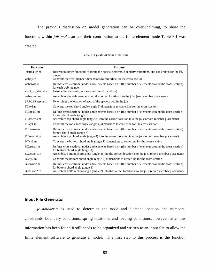
93
The previous discussion on model generation can be overwhelming, to show the
functions within joistmaker.m and their contribution to the finite element mode Table F.1 was
created.
Table F.1 joistmaker.m Functions
Function Purpose joistmaker.m References other functions to create the nodes, elements, boundary conditions, and constraints for the FE
model webxy.m Converts the web-member dimensions to centerline for the cross-section
webcross.m Defines cross sectional nodes and elements based on n (the number of elements around the cross-section) for each web member
xsect_to_abaqus.m Extrude the element (both web and chord members)
webassem.m Assembles the web members into the correct location into the joist (web member placement)
SPACERassem.m Determines the location of each of the spacers within the joist
TCxy3.m Converts the top chord angle (angle 3) dimensions to centerline for the cross-section
TCcross3.m Defines cross sectional nodes and elements based on n (the number of elements around the cross-section) for top chord angle (angle 3)
TCassem3.m Assembles top chord angle (angle 3) into the correct location into the joist (chord member placement)
TCxy4.m Converts the top chord angle (angle 4) dimensions to centerline for the cross-section
TCcross4.m Defines cross sectional nodes and elements based on n (the number of elements around the cross-section) for top chord angle (angle 4)
TCassem4.m Assembles top chord angle (angle 4) into the correct location into the joist (chord member placement)
BCxy1.m Converts the bottom chord angle (angle 1) dimensions to centerline for the cross-section
BCcross1.m Defines cross sectional nodes and elements based on n (the number of elements around the cross-section) for bottom chord angle (angle 1)
BCassem1.m Assembles bottom chord angle (angle 4) into the correct location into the joist (chord member placement)
BCxy2.m Converts the bottom chord angle (angle 2) dimensions to centerline for the cross-section
BCcross2.m Defines cross sectional nodes and elements based on n (the number of elements around the cross-section) for bottom chord angle (angle 2)
BCassem2.m Assembles bottom chord angle (angle 2) into the correct location into the joist (chord member placement)
Input File Generator
joistmaker.m is used to determine the node and element location and numbers,
constraints, boundary conditions, spring locations, and loading conditions; however, after this
information has been found it still needs to be organized and written to an input file to allow the
finite element software to generate a model. The first step to this process is the function

94
nlbatchr4.m which references joistmaker.m, relays this information to other functions, which
write different sections of the input file, before model generation can be completed.
The first step to this process is to determine the clip stiffness, see Chapter 4, and input
that into nlbatch4r.m, along with the job name (which will be the name of the finite element
model). The other initial input is the analysis type for which there are two choices, collapse
analysis (denoted by inputting ‘C’) or a buckling analysis (denoted by inputting ‘B’).
nlbatchr4.m will then automatically pull in the necessary information from joistmaker.m to allow
the input file to be written.
When performing a collapse analysis it is important to have plastic material behavior
included in the model. This is possible to enter under the variable matprops(1).plastic in
nlbatch4r.m where the first column represents stress and the second column represents strain past
the yield point (the first point should be the yield stress and zero strain). This information should
be gathered from a tensile test of the failing material, in the case of the Virginia Tech tests top
chord material was used.
It is important to note that many of the inputs in this section are written within quotes.
The purpose of this is to write the information to the input file, any text written inside of quotes
will be written as text into the input file.
To control the analysis steps a matrix is provided that allows the user to input the steps
required by the Riks analysis in ABAQUS. The Riks steps in ABAQUS are the initial increment
arc length, the total arc length scale factor, the minimum arc length increment, the maximum arc
length increment, and the maximum load proportionality factor, if this any of this information is
neglected ABAQUS will use default information for analysis, see the ABAQUS documentation
for more information. These values can be entered under the step(1).solutionsteps variable;
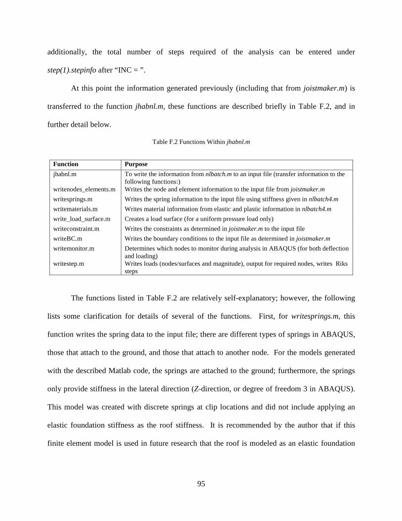
95
additionally, the total number of steps required of the analysis can be entered under
step(1).stepinfo after “INC = ”.
At this point the information generated previously (including that from joistmaker.m) is
transferred to the function jhabnl.m, these functions are described briefly in Table F.2, and in
further detail below.
Table F.2 Functions Within jhabnl.m
Function Purpose
jhabnl.m To write the information from nlbatch.m to an input file (transfer information to the following functions:)
writenodes_elements.m Writes the node and element information to the input file from joistmaker.m
writesprings.m Writes the spring information to the input file using stiffness given in nlbatch4.m
writematerials.m Writes material information from elastic and plastic information in nlbatch4.m
write_load_surface.m Creates a load surface (for a uniform pressure load only)
writeconstraint.m Writes the constraints as determined in joistmaker.m to the input file
writeBC.m Writes the boundary conditions to the input file as determined in joistmaker.m
writemonitor.m Determines which nodes to monitor during analysis in ABAQUS (for both deflection and loading)
writestep.m Writes loads (nodes/surfaces and magnitude), output for required nodes, writes Riks steps
The functions listed in Table F.2 are relatively self-explanatory; however, the following
lists some clarification for details of several of the functions. First, for writesprings.m, this
function writes the spring data to the input file; there are different types of springs in ABAQUS,
those that attach to the ground, and those that attach to another node. For the models generated
with the described Matlab code, the springs are attached to the ground; furthermore, the springs
only provide stiffness in the lateral direction (Z-direction, or degree of freedom 3 in ABAQUS).
This model was created with discrete springs at clip locations and did not include applying an
elastic foundation stiffness as the roof stiffness. It is recommended by the author that if this
finite element model is used in future research that the roof is modeled as an elastic foundation

96
rather than with discrete springs; this can be accomplished using the *FOUNDATION command
in ABAQUS, for more information see the ABAQUS documentation.
For the file writeBC.m, it is important to include the correct degrees of freedom to be
restrained. The translational degrees of freedom in ABAQUS are 1, 2, and 3, for the X, Y, and Z
directions respectively; similarly, the rotational degrees of freedom are 4, 5, and 6, for the same
directions. For the models created at Virginia Tech simple supports were used, these should be
altered for other boundary conditions.
To analyze the results from the models it was necessary to track the displacement and the
load on the joists. To track the load the node that was the closest to midspan in one of the angles
of the bottom chord was found in the function BCassem1.m and transferred to writemonitor.m
(which simply writes this node (or nodes for multiple joists) into the ABAQUS input file). Load
was applied as even point loads at clip locations which made tracking the load easy; it was
possible to monitor a single node where load was applied to determine the total load on the joist.
The first node from the point load node set was taken to monitor the load, this can be found in
the writestep.m function. From this point it was possible to compare load and displacement and
determine when failure occurred for an easy comparison to the laboratory test data.
The function writestep.m controls writing all of the analysis steps to the input file. This
includes writing the steps for the Riks analysis, setting the nodes (or elements) to which the load
is applied, setting the maximum load magnitude and direction, and setting the nodes to monitor
for load and displacement and write these values to the .dat file for post-processing.
Figure F.5 displays a flowchart that shows the process of model generation and the
progression of functions created to establish a finite element model.
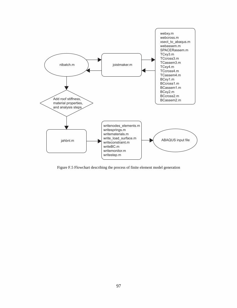
97
Figure F.5 Flowchart describing the process of finite element model generation
nlbatch.m joistmaker.m
webxy.m
webcross.m
xsect_to_abaqus.m
webassem.m
SPACERassem.m
TCxy3.m
TCcross3.m
TCassem3.m
TCxy4.m
TCcross4.m
TCassem4.m
BCxy1.m
BCcross1.m
BCassem1.m
BCxy2.m
BCcross2.m
BCassem2.mAdd roof stiffness,
material properties,
and analysis steps
jahbnl.m
writenodes_elements.m
writesprings.m
writematerials.m
write_load_surface.m
writeconstraint.m
writeBC.m
writemonitor.m
writestep.m
ABAQUS input file
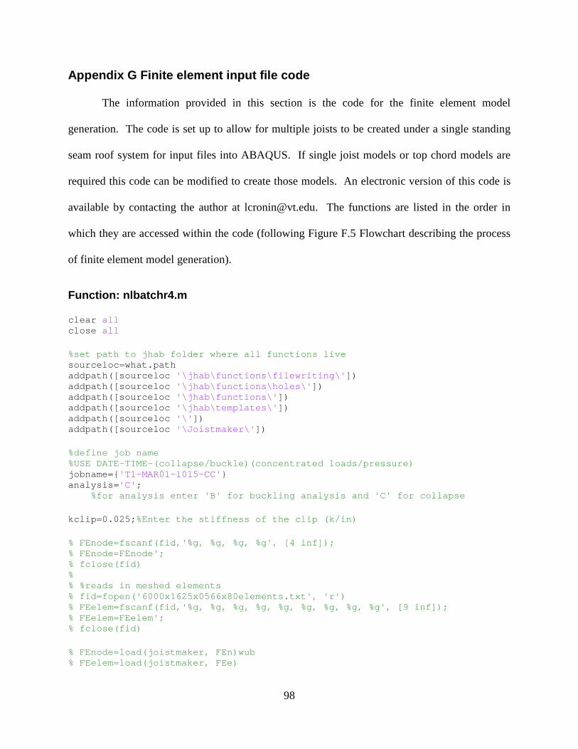
98
Appendix G Finite element input file code
The information provided in this section is the code for the finite element model
generation. The code is set up to allow for multiple joists to be created under a single standing
seam roof system for input files into ABAQUS. If single joist models or top chord models are
required this code can be modified to create those models. An electronic version of this code is
available by contacting the author at [email protected]. The functions are listed in the order in
which they are accessed within the code (following Figure F.5 Flowchart describing the process
of finite element model generation).
Function: nlbatchr4.m
clear all close all %set path to jhab folder where all functions live sourceloc=what.path addpath([sourceloc '\jhab\functions\filewriting\' ]) addpath([sourceloc '\jhab\functions\holes\' ]) addpath([sourceloc '\jhab\functions\' ]) addpath([sourceloc '\jhab\templates\' ]) addpath([sourceloc '\' ]) addpath([sourceloc '\Joistmaker\' ]) %define job name %USE DATE-TIME-(collapse/buckle)(concentrated loads /pressure) jobname={ 'T1-MAR01-1015-CC' } analysis= 'C' ; %for analysis enter 'B' for buckling analysis and ' C' for collapse kclip=0.025; %Enter the stiffness of the clip (k/in) % FEnode=fscanf(fid,'%g, %g, %g, %g', [4 inf]); % FEnode=FEnode'; % fclose(fid) % % %reads in meshed elements % fid=fopen('6000x1625x0566x80elements.txt', 'r') % FEelem=fscanf(fid,'%g, %g, %g, %g, %g, %g, %g, %g , %g', [9 inf]); % FEelem=FEelem'; % fclose(fid) % FEnode=load(joistmaker, FEn)wub % FEelem=load(joistmaker, FEe)
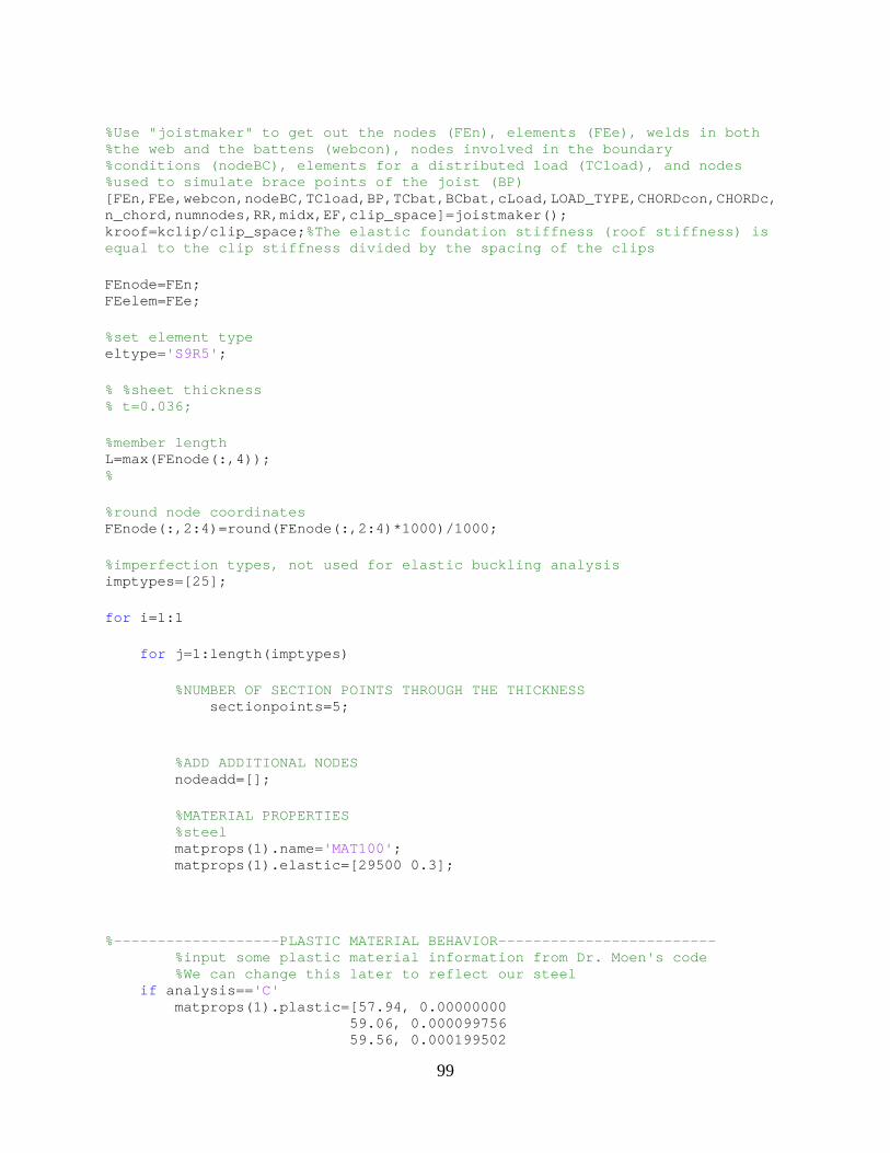
99
%Use "joistmaker" to get out the nodes (FEn), eleme nts (FEe), welds in both %the web and the battens (webcon), nodes involved i n the boundary %conditions (nodeBC), elements for a distributed lo ad (TCload), and nodes %used to simulate brace points of the joist (BP) [FEn,FEe,webcon,nodeBC,TCload,BP,TCbat,BCbat,cLoad, LOAD_TYPE,CHORDcon,CHORDc,n_chord,numnodes,RR,midx,EF,clip_space]=joistmaker( ); kroof=kclip/clip_space; %The elastic foundation stiffness (roof stiffness) is equal to the clip stiffness divided by the spacing of the clips FEnode=FEn; FEelem=FEe; %set element type eltype= 'S9R5' ; % %sheet thickness % t=0.036; %member length L=max(FEnode(:,4)); % %round node coordinates FEnode(:,2:4)=round(FEnode(:,2:4)*1000)/1000; %imperfection types, not used for elastic buckling analysis imptypes=[25]; for i=1:1 for j=1:length(imptypes) %NUMBER OF SECTION POINTS THROUGH THE THICKNESS sectionpoints=5; %ADD ADDITIONAL NODES nodeadd=[]; %MATERIAL PROPERTIES %steel matprops(1).name= 'MAT100' ; matprops(1).elastic=[29500 0.3]; %-------------------PLASTIC MATERIAL BEHAVIOR------ ------------------- %input some plastic material information from Dr. M oen's code %We can change this later to reflect our steel if analysis== 'C' matprops(1).plastic=[57.94, 0.00000000 59.06, 0.000099756 59.56, 0.000199502
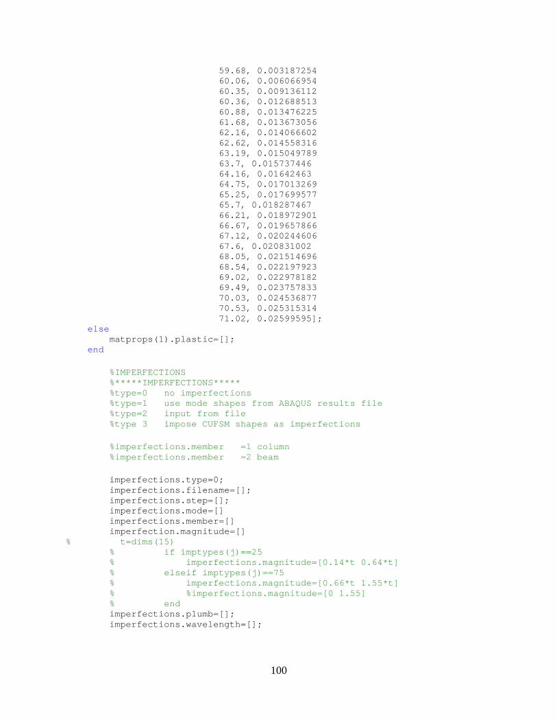
100
59.68, 0.003187254 60.06, 0.006066954 60.35, 0.009136112 60.36, 0.012688513 60.88, 0.013476225 61.68, 0.013673056 62.16, 0.014066602 62.62, 0.014558316 63.19, 0.015049789 63.7, 0.015737446 64.16, 0.01642463 64.75, 0.017013269 65.25, 0.017699577 65.7, 0.018287467 66.21, 0.018972901 66.67, 0.019657866 67.12, 0.020244606 67.6, 0.020831002 68.05, 0.021514696 68.54, 0.022197923 69.02, 0.022978182 69.49, 0.023757833 70.03, 0.024536877 70.53, 0.025315314 71.02, 0.02599595]; else matprops(1).plastic=[]; end %IMPERFECTIONS %*****IMPERFECTIONS***** %type=0 no imperfections %type=1 use mode shapes from ABAQUS results file %type=2 input from file %type 3 impose CUFSM shapes as imperfections %imperfections.member =1 column %imperfections.member =2 beam imperfections.type=0; imperfections.filename=[]; imperfections.step=[]; imperfections.mode=[] imperfections.member=[] imperfection.magnitude=[] % t=dims(15) % if imptypes(j)==25 % imperfections.magnitude=[0.14*t 0.64* t] % elseif imptypes(j)==75 % imperfections.magnitude=[0.66*t 1.55* t] % %imperfections.magnitude=[0 1.55] % end imperfections.plumb=[]; imperfections.wavelength=[];

101
nodesetinfo={ }; %DEFINE SPRINGS springs=[] %DEFINE CONTACT SURFACES, NODE SURFACES, KINEMATIC CONSTRAINTS,.... surface.type={} surface.type=[] surface.local=[] surface.coord=[] %set up warping fixed boundary conditions surface.coupling={}; surface.interaction=[] surface.contact=[] surface.areadist=[] %DEFINE ANALYSIS STEP surface.type={ '*Surface, Name=LEFTS, Type=Node' 'ENDXZERO' ' ' } surface.local=[] surface.coord=[] surface.coupling=[{ '*Coupling, Constraint Name=LEFTC, Ref Node=SHEARCENTER,Surface=LEFTS' , '*Kinematic' , '1,2' }]; surface.interaction=[] surface.contact=[] surface.areadist=[] %DEFINE ANALYSIS STEP %make this into two pieces, one for each type of an alysis if analysis== 'B' step(1).stepinfo={ 'STEP 1,' 'perturbation' []}; step(1).solutiontype= 'Buckle, eigensolver=lanczos' ; step(1).solutionsteps={ '50, , ,' }; step(1).solutioncontrols={ }; step(1).coupling=[] step(1).loads={} step(1).loads={} step(1).outrequest={ '*Output, field, variable=PRESELECT' ;} % '*Node Print, NSET=ROT, SUMMARY=NO'; % 'U3'; % '*Node Print, NSET=SHEARCENTER, SUMMARY=N O'; % 'UR1,RM1'} nele=length(FEelem(:,1)) node=[] elem=[] else %The following values are updated to always work wi th the last running

102
%collapse model step(1).stepinfo={ 'STEP 1,' 'nlgeom, INC=75' []}; step(1).solutiontype= 'Static, Riks' ; step(1).solutionsteps={ '1.000000e-02,,1.000000e-12,, , , , ,' }; %Here are the defaults for solutionsteps %1.000000e-002, ,1.000000e-010,1.000000e-002, , , , , %The first line of *STATIC, RIKS are: % initial increment arc length, total arc length scale factor, minimum arc length increment, maximum arc length in crement, maximum load prop. factor %you need to figure something out for yourself step(1).solutioncontrols={ }; step(1).coupling=[] step(1).loads={} step(1).loads={} %Frequency=10 gives 10 points in the ODB file inste ad of the default of %20. This greatly reduces the file size, for this f ile it reduces it to %less than 1 GB compared a 8-12 GB file without it %This is controlled in the file: 'writestep.m' % step(1).outrequest={'*Output, field, variable =PRESELECT, frequency=10'; % '*Node Print, NSET=ROT, SUMMARY=NO'; % 'U3'; % '*Node Print, SUMMARY=NO'} nele=length(FEelem(:,1)) node=[] elem=[] end disp( 'Input Complete...starting model generation' ); %WRITE ABAQUS INP FILE %this is the important function, you can use this i n for loops to generate parameter studies jhabnl(step, jobname{i},matprops,imperfecti ons,sectionpoints, FEnode, FEelem, eltype, webcon, nodeBC,TCload,BP,TCbat,BCbat,cLoad,LOAD_TYPE,CHORDc on,CHORDc,n_chord,numnodes,analysis,kclip,RR,midx,EF,kroof) end end
Function: joistmaker.m
function [FEn,FEe,webcon,nodeBC,TCload,BP,TCbat,BCbat,cLoad, LOAD_TYPE,CHORDcon,CHORDc,n_chord,numnodes,RR,midx,EF,clip_space]=joi stmaker()
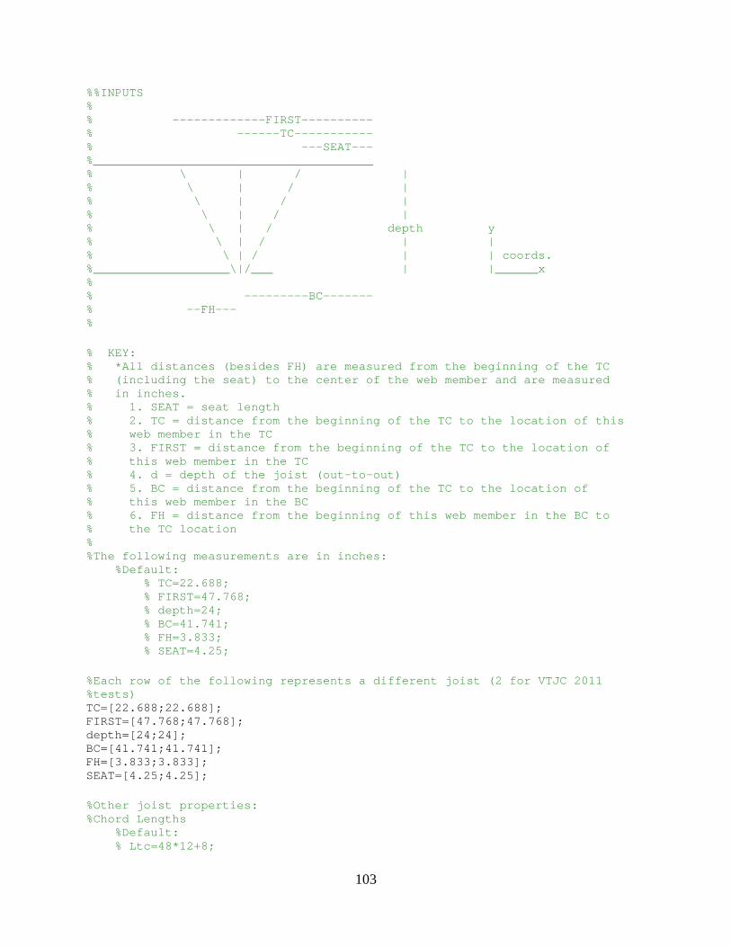
103
%%INPUTS % % -------------FIRST---------- % ------TC----------- % ---SEAT--- %_______________________________________ % \ | / | % \ | / | % \ | / | % \ | / | % \ | / depth y % \ | / | | % \ | / | | coords. %___________________\|/___ | |______x % % ---------BC------- % --FH--- % % KEY: % *All distances (besides FH) are measured from t he beginning of the TC % (including the seat) to the center of the web m ember and are measured % in inches. % 1. SEAT = seat length % 2. TC = distance from the beginning of the TC to the location of this % web member in the TC % 3. FIRST = distance from the beginning of the TC to the location of % this web member in the TC % 4. d = depth of the joist (out-to-out) % 5. BC = distance from the beginning of the TC to the location of % this web member in the BC % 6. FH = distance from the beginning of this w eb member in the BC to % the TC location % %The following measurements are in inches: %Default: % TC=22.688; % FIRST=47.768; % depth=24; % BC=41.741; % FH=3.833; % SEAT=4.25; %Each row of the following represents a different j oist (2 for VTJC 2011 %tests) TC=[22.688;22.688]; FIRST=[47.768;47.768]; depth=[24;24]; BC=[41.741;41.741]; FH=[3.833;3.833]; SEAT=[4.25;4.25]; %Other joist properties: %Chord Lengths %Default: % Ltc=48*12+8;

104
% %Global test properties Ltc=48*12+8; %Length of the top chord in inches including seat Number_Joists=2; %The number of joists in model Joist_Space=5*12; %The center-to-center spacing of the joists % %Local joist properties (within each joist) SPACE=1; %the space between each of the web members in a gro up at the beginning/end GAP=0.25; %the space between each of the web members in major ity of the joist change=1; %the depth of the web member will always be less th an the depth of the joist, this value tells you by what amount BracePts=0; %The number of brace points along the joist %Imperfections & Camber imp_amp=[2.411;1.5715]; %The imperfection magnitude of each joist is represented by its row location (1st row=1st joist, 2nd row=2nd joist, etc.) %if both imperfection amplitudes have the same sign they will %be in the same direction and vice versa camber=[0.75;0.75]; %The maximum amount of camber at mid-span %LOAD TYPE - 'P' = pressure, 'C' = concentrated loa d (at clip locations) LOAD_TYPE='C' ; % Lbc=498; %Length of the bottom chord in inches %Clip locations FCL=24; %location of the first clip from the end of the joi st (in) clip_space=24; %Spacing of the clips (in) %Make a global loop to allow for multiple joists to be produced %Move the origin based on what joist you are on for ii=1:Number_Joists origin=0+Joist_Space*(ii-1); %% %Change inputs so they are only the x-component of the web member and do %not include the seat BC(ii)=BC(ii,1)-SEAT(ii,1); TC(ii)=TC(ii,1)-SEAT(ii,1); FIRST(ii)=FIRST(ii,1)-SEAT(ii,1); %make an array of lengths so the correct length can be extruded for each web member Length=[sqrt((2*((depth(ii,1)-SPACE)^2))) %45 degree members sqrt((BC(ii,1)-SPACE-GAP)^2+(depth(ii,1))^2 ) %outermost members sqrt((BC(ii,1)-SPACE-TC(ii,1))^2+depth(ii,1 )^2) %2nd outermost members sqrt((depth(ii,1)^2+(FH(ii,1))^2)) %3rd outermost members depth(ii,1)]; %vertical members %% %cross sectional dimensions
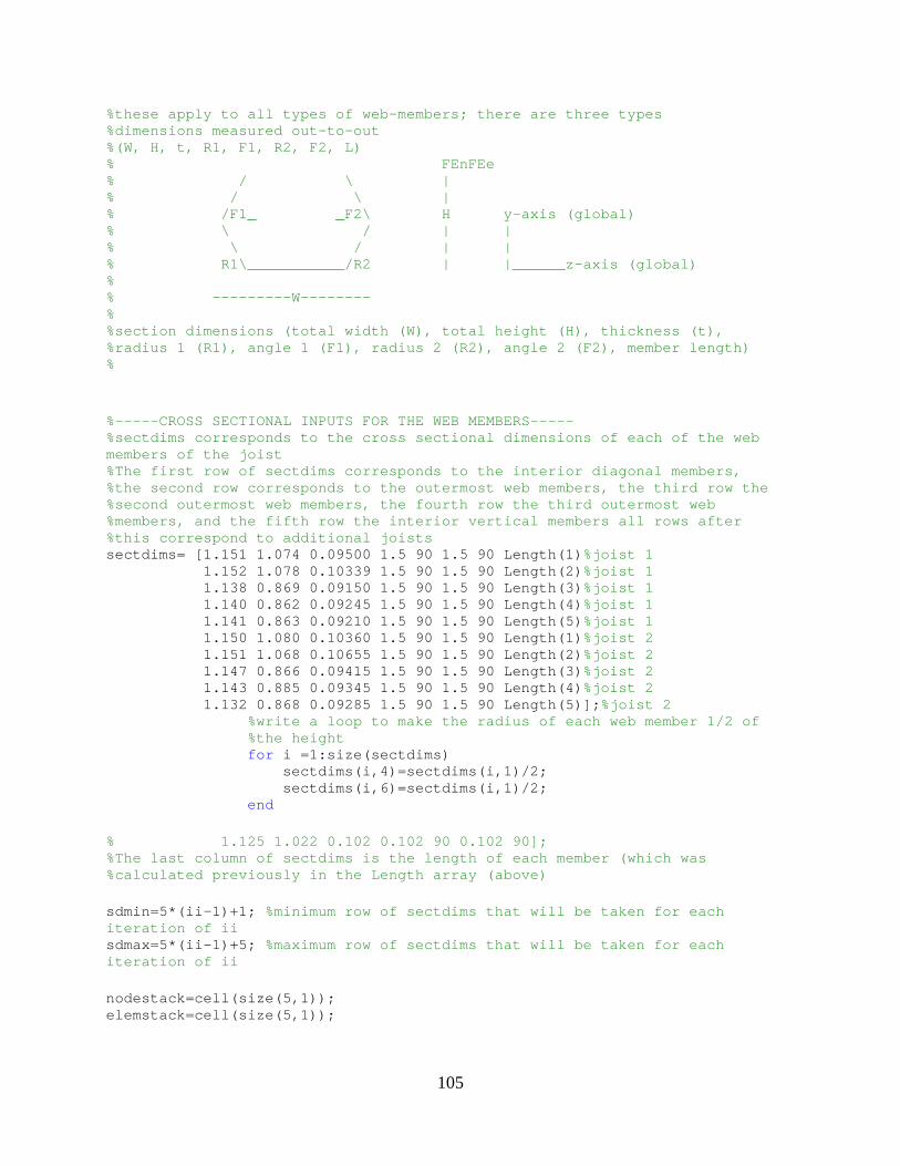
105
%these apply to all types of web-members; there are three types %dimensions measured out-to-out %(W, H, t, R1, F1, R2, F2, L) % FEnFEe % / \ | % / \ | % /F1_ _F2\ H y-axis (global) % \ / | | % \ / | | % R1\___________/R2 | |_____ _z-axis (global) % % ---------W-------- % %section dimensions (total width (W), total height (H), thickness (t), %radius 1 (R1), angle 1 (F1), radius 2 (R2), angle 2 (F2), member length) % %-----CROSS SECTIONAL INPUTS FOR THE WEB MEMBERS--- -- %sectdims corresponds to the cross sectional dimens ions of each of the web members of the joist %The first row of sectdims corresponds to the inter ior diagonal members, %the second row corresponds to the outermost web me mbers, the third row the %second outermost web members, the fourth row the t hird outermost web %members, and the fifth row the interior vertical m embers all rows after %this correspond to additional joists sectdims= [1.151 1.074 0.09500 1.5 90 1.5 90 Length (1) %joist 1 1.152 1.078 0.10339 1.5 90 1.5 90 Length (2) %joist 1 1.138 0.869 0.09150 1.5 90 1.5 90 Length (3) %joist 1 1.140 0.862 0.09245 1.5 90 1.5 90 Length (4) %joist 1 1.141 0.863 0.09210 1.5 90 1.5 90 Length (5) %joist 1 1.150 1.080 0.10360 1.5 90 1.5 90 Length (1) %joist 2 1.151 1.068 0.10655 1.5 90 1.5 90 Length (2) %joist 2 1.147 0.866 0.09415 1.5 90 1.5 90 Length (3) %joist 2 1.143 0.885 0.09345 1.5 90 1.5 90 Length (4) %joist 2 1.132 0.868 0.09285 1.5 90 1.5 90 Length (5)]; %joist 2 %write a loop to make the radius of each web member 1/2 of %the height for i =1:size(sectdims) sectdims(i,4)=sectdims(i,1)/2; sectdims(i,6)=sectdims(i,1)/2; end % 1.125 1.022 0.102 0.102 90 0.102 90]; %The last column of sectdims is the length of each member (which was %calculated previously in the Length array (above) sdmin=5*(ii-1)+1; %minimum row of sectdims that will be taken for eac h iteration of ii sdmax=5*(ii-1)+5; %maximum row of sectdims that will be taken for eac h iteration of ii nodestack=cell(size(5,1)); elemstack=cell(size(5,1));
106
depth=depth-change; %the depth of the web member will always be less th an the depth of the joist tick=1; %Make a counter to use to count the web members mad e for each joist %This is where the web members are made (in their o wn local coordinates) for i=sdmin:1:sdmax L=sectdims(i,8); H=sectdims(sdmin:1:sdmax,2); W=sectdims(1,1); %The total width of the web members, this should be consistent for all (it will need to change otherwis e) %make each iteration have a separate nodestack (we are going to need %two loops) % %The second loop should include the assembly %Mesh along length nele=L; dims=sectdims(i,:); %Create the number of section points through the th ickness sectionpoints=5; %Cross-section meshing %number of elements around the cross section n=[2 4 0 4 2]; N=n(1,1)+n(1,2)+n(1,3)+n(1,4)+n(1,5)+1; %the total number of nodes in each cross section %convert to centerline dimensions for the cross sec tion [xy]=webxy(dims); %define nodes, elements and properties in CUFSM coo rds. kipin=1; [node, elem]=webcross(xy, dims, kipin, n); %plot node to check % figure(i) % plot(node(:,2), node(:,3),'k.') % %extrude the element using xsect [FEnode,FEelem,t,matnum,nnodes,nL,FEsection_increme nt,elemgroups,node]=xsect_to_abaqus(L, nele, node, elem); %We can change the z-coordinate here to allow for m ultiple joists to be %produced (just add the spacing of the joist to FEn ode and FEelem) FEnode(:,4)=FEnode(:,4)+origin; %plot 3D to see extrusion along the length of the m ember
107
% figure(i+10) % plot3(FEnode(:,2),FEnode(:,4),FEnode(:,3),'k. ') % FEnode % FEelem %create an array of FEnode and FEelem so we can use them later in assembly nodestack{tick}=FEnode; elemstack{tick}=FEelem; tstack{tick}=sectdims(i,3); tick=tick+1; end %----------------ASSEMBLE WEB MEMBERS INTO THE JOIS T---------------- %Create a value for the following so MATLAB does no t freak out--for the %first iteration (first joist) only if ii==1 FEn=0; FEe=0; cLoad=0; CHORDcount=0; pinend=0; %And now the cells: midx{1}=0; RR{1}=0; webcon{1}=0; TCload{1}=0; nodeBC{1}=0; BP{1}=0; TCbat{1}=0; BCbat{1}=0; EF{1}=0; end %This is where the web members are rotated and plac ed along the length of %the joist %Find FEnode (FEn) and FEelem (FEe) for the web mem bers [FEn,FEe,webcon,numdiag,numnodes,pinend]=webassem(n odestack, elemstack, tstack, sectdims, TC, FIRST, depth, BC, FH, SEAT, L tc, change,SPACE,GAP,H,N,FEn,FEe,ii,webcon,pinend); %% % ---------------INPUTS FOR THE CHORD MEMBERS------ -------------- depth=depth+change; % Dimensions are measured from the intersection of the height and width to % the ends of the angle % %section dimensions (per angle): angle width (W), a ngle height(H), %thickness(t), outside radius(R), angle of W-H inte rsection (degrees)(F) % %S is the distance between the two angles, measured between the %intersection of the H and W legs of each angle %

108
%d is the depth of the section (measured out-to-out ) - d should be measured %from angle #1 to angle #3 % % [W1, H1, t1, R1, F1, W2, H2, t2, R2, F2, S1, W3, H3, t3, R3, F3, W4, H4, t4, R4, F4, S2, d] %Cross-section dimensions % % S2 % ___W4____R4 R5____W3____ % F4/ \F3 | % / \ | % /H4 H3\ | % / \ | % / \ | % t4 t3 | % | % d % | % | % t2 t1 | % \ / | % \ / | % \H2 H1 / ^ | % \ / | | % \ / y-axis | % _______F2\R2 R1/_F1_______ |__z-axis__> | % W2 S1 W1 %TCdims % [W1, H1, t1, R1, F1, W2, H2, t2, R2, F2, S1] %BCdims % [W3, H3, t3, R3, F3, W4, H4, t4, R4, F4, S2, d] %top chord dimensions: %Where %TCdims are as follows: %row 1 - Joist 1 %row 2 - Joist 2 TCdims=[1.504 1.508 .1490 0 90 1.504 1.501 0.13785 0 90 1.125 depth(ii) 1.502 1.506 .1487 0 90 1.505 1.503 0.13990 0 90 1.125 depth(ii)]; %rewrite the radius to be equal to the member thick ness for i=1:size(TCdims) TCdims(i,4)=TCdims(i,3); TCdims(i,9)=TCdims(i,8); end %TCdims are as follows: %row 1 - Joist 1 %row 2 - Joist 2 %Bottom chord dimensions BCdims=[1.519 1.480 0.14900 0 90 1.504 1.501 0.1378 5 0 90 1.125 1.529 1.501 0.14195 0 90 1.498 1.508 0.1403 5 0 90 1.125];

109
%rewrite the radius to be equal to the member thick ness for i=1:size(TCdims) BCdims(i,4)=BCdims(i,3); BCdims(i,9)=BCdims(i,8); end % Lbc=498; %length for the bottom chord % ---------------PLACE THE SPACERS MEMBERS--------- ----------- %Spacers are the small angles that are placed in be tween angles %along the length of the chord, between web members % R % | /\ % | /F \ % H / \ y % | / \ | coords. % | / \ |____z % t % ----W----- %SPACERdims % [W, H, t, R, F] %Batten dimensions SPACERdims=[1.75 1.75 0.1 0.1 90]; %% %-------SPACER EXTRUSION----- tick=1; for i=1:size(SPACERdims) %Member length H=SPACERdims(1,2); L=TCdims(1,11); %length of the batten is equal to the space in between the chords %!!!!!!!!!!!!!!!!!!!!!THIS NEEDS TO CHANGE IF WE MA KE MULTIPLE %JOISTS!!!!!!!!!! %Mesh along length nele=L; %Create the number of section points through the th ickness sectionpoints=5; %Cross-section meshing %number of elements around the cross section %[H, R, W] n=[4 4 4]; N=n(1,1)+n(1,2)+n(1,3);

110
dims=SPACERdims(i,:); %convert to centerline dimensions for the cross sec tion [xy]=battenxy(dims); %Define nodes, elements and properties in CUFSM %kipin gives material properties, we need to input this whenever we %figure out what our material properties are kipin=1; [node, elem]=battencross1(xy, dims, kipin,n ); %plot node to check % figure(i) % plot3(node(:,2),node(:,4),node(:,3),'k.') %extrude the element using xsect [FEnode,FEelem,t,matnum,nnodes,nL,FEsection_increme nt,elemgroups,node]=xsect_to_abaqus(L, nele, node, elem); %We can change the z-coordinate here to allow for m ultiple joists to be %produced (just add the spacing of the joist to FEn ode and FEelem) FEnode(:,4)=FEnode(:,4)+origin; %plot 3d to check % figure(i+10) % plot3(FEnode(:,2),FEnode(:,4),FEnode(:,3),'k. ') %create an array of FEnode and FEelem so we can use them later in assembly %However, for this initial program just use one joi st nodestack{tick}=FEnode; elemstack{tick}=FEelem; tstack{tick}=[SPACERdims(i,3)]; tick=tick+1; end %-------------ASSEMBLE SPACERS INTO THE JOIST------ ------- if ii==1 %only assemble the spacers based on the location of the first joist because all other spacers will have the same x-loca tion [FEn,FEe,TCbatpos,BCbatpos,numbattens]=SPACERassem( nodestack,FEn,FIRST,SEAT,depth,GAP,FEe,elemstack,tstack,Ltc,webcon,N,H,numdia g,ii); end %% %-------TOP CHORD EXTRUSION----- sdmin=1*(ii-1)+1; %minimum row of sectdims that will be taken for eac h iteration of ii tick=1;
111
%For angle #3 for i=sdmin:sdmin %one top chord per joist %Member length L=Ltc; %length of the top chord %Mesh along length nele=L; %Create the number of section points through the th ickness sectionpoints=5; %Cross-section meshing %number of elements around the cross section %[W, R, H] n=[4 2 4]; N=n(1,1)+n(1,2)+n(1,3); %The total number of elements per cross section n_chord=n; dims=TCdims(i,:); s=TCdims(i,11); %convert to centerline dimensions for the cross sec tion [xy]=TCxy3(dims); %Define nodes, elements and properties in CUFSM %kipin gives material properties, we need to input this whenever we %figure out what our material properties are kipin=1; [node, elem]=TCcross3(xy, dims, kipin,n); %plot node to check % figure(i) % plot3(node(:,2),node(:,4),node(:,3),'k.') %extrude the element using xsect [FEnode,FEelem,t,matnum,nnodes,nL,FEsection_increme nt,elemgroups,node]=xsect_to_abaqus(L, nele, node, elem); %We can change the z-coordinate here to allow for m ultiple joists to be %produced (just add the spacing of the joist to FEn ode and FEelem) FEnode(:,4)=FEnode(:,4)+origin; %plot 3d to check % figure(i+10) % plot3(FEnode(:,2),FEnode(:,4),FEnode(:,3),'k. ') %create an array of FEnode and FEelem so we can use them later in assembly
112
%However, for this initial program just use one joi st nodestack{tick}=FEnode; elemstack{tick}=FEelem; tstack{tick}=[TCdims(i,3)]; tick=tick+1; end %-------------ASSEMBLE angle #3 INTO THE JOIST----- -------- [FEn,FEe,nodeBC,TCload,BP,TCbat,cLoad,CHORDcon,CHOR Dcount,RR,EF]=TCassem3(nodestack,elemstack,tstack,FEn,FEe,s,depth,change,SEAT ,Ltc,N,n,BracePts,TCbatpos,numbattens,LOAD_TYPE,webcon,W,ii,cLoad,TCload,node BC,BP,TCbat,CHORDcount,pinend,FCL,clip_space,RR,EF); tick=1; %For angle #4 for i=sdmin:sdmin %2 angles per bottom chord %Member length L=Ltc; %length of the top chord %Mesh along length nele=L; %Create the number of section points through the th ickness sectionpoints=5; %Cross-section meshing %number of elements around the cross section %[H, R, W] n=[4 2 4]; N=n(1,1)+n(1,2)+n(1,3); dims=TCdims(i,:); s=TCdims(i,11); %convert to centerline dimensions for the cross sec tion [xy]=TCxy4(dims); %Define nodes, elements and properties in CUFSM %kipin gives material properties, we need to input this whenever we %figure out what our material properties are kipin=1; [node, elem]=TCcross4(xy, dims, kipin,n); %plot node to check % figure(i) % plot3(node(:,2),node(:,4),node(:,3),'k.') %extrude the element using xsect [FEnode,FEelem,t,matnum,nnodes,nL,FEsection_increme nt,elemgroups,node]=xsect_to_abaqus(L, nele, node, elem);
113
%We can change the z-coordinate here to allow for m ultiple joists to be %produced (just add the spacing of the joist to FEn ode and FEelem) FEnode(:,4)=FEnode(:,4)+origin; %plot 3d to check % figure(i+10) % plot3(FEnode(:,2),FEnode(:,4),FEnode(:,3),'k. ') %create an array of FEnode and FEelem so we can use them later in assembly %However, for this initial program just use one joi st nodestack{tick}=FEnode; elemstack{tick}=FEelem; tstack{tick}=[TCdims(i,8)]; tick=tick+1; end %-------------ASSEMBLE angle #4 INTO THE JOIST----- -------- [FEn,FEe,nodeBC,TCload,BP,TCbat,CHORDcon,CHORDcount ,cLoad,RR]=TCassem4(nodestack,elemstack,tstack,FEn,FEe,s,depth,change,SEAT,no deBC,N,n,TCload,Ltc,BracePts,TCbatpos,numbattens,BP,TCbat,webcon,W,CHORDcon,C HORDcount,ii,cLoad,pinend,FCL,clip_space,RR); %plot to check % figure(2) % plot(FEn(:,2),FEn(:,3),'k.') % %% %-------BOTTOM CHORD EXTRUSION----- tick=1; %For angle #1 for i=sdmin:sdmin %Number of diagonals per 1/2 span numdiag=round(((Ltc-2*SEAT(ii,1)-2*FIRST(ii,1))/(depth(ii,1)))*1/2); %the number of diagonals in the joist (for each 45 degree orientation) %Member length L=Ltc-2*(SEAT(ii,1)+BC(ii,1))+numdiag* 3*GAP-4*SPACE; %length of the bottom chord %Mesh along length nele=L; %Create the number of section points through the th ickness sectionpoints=5; %Cross-section meshing %number of elements around the cross section %[H, R, W]
114
n=[4 2 4]; dims=BCdims(i,:); s=BCdims(i,11); %convert to centerline dimensions for the cross sec tion [xy]=BCxy1(dims); %Define nodes, elements and properties in CUFSM %kipin gives material properties, we need to input this whenever we %figure out what our material properties are kipin=1; [node, elem]=BCcross1(xy, dims, kipin,n ); %plot node to check % figure(i) % plot3(node(:,2),node(:,4),node(:,3),'k.') %extrude the element using xsect [FEnode,FEelem,t,matnum,nnodes,nL,FEsection_increme nt,elemgroups,node]=xsect_to_abaqus(L, nele, node, elem); %We can change the z-coordinate here to allow for m ultiple joists to be %produced (just add the spacing of the joist to FEn ode and FEelem) FEnode(:,4)=FEnode(:,4)+origin; %plot 3d to check % figure(i+10) % plot3(FEnode(:,2),FEnode(:,4),FEnode(:,3),'k. ') %create an array of FEnode and FEelem so we can use them later in assembly %However, for this initial program just use one joi st nodestack{tick}=FEnode; elemstack{tick}=FEelem; tstack{tick}=BCdims(i,3); tick=tick+1; end %-------------ASSEMBLE angle #1 INTO THE JOIST----- -------- [FEn,FEe,BP,BCbat,CHORDcon,CHORDcount,nodeBC,midx]= BCassem1(nodestack,elemstack,tstack,FEn,FEe,BC,s,depth,change,SEAT,SPACE,GAP, Ltc,BracePts,BCbatpos,numbattens,BP,webcon,W,CHORDcon,CHORDcount,ii,BCbat,N,n odeBC,pinend,midx,n); tick=1; %For angle #2 for i=sdmin:sdmin

115
%Member length L=Ltc-2*(SEAT(ii,1)+BC(ii,1))+numdiag* 3*GAP-4*SPACE; %length of the bottom chord %Mesh along length nele=L; %Create the number of section points through the th ickness sectionpoints=5; %Cross-section meshing %number of elements around the cross section %[H, R, W] n=[4 2 4]; dims=BCdims(i,:); %convert to centerline dimensions for the cross sec tion [xy]=BCxy2(dims); %Define nodes, elements and properties in CUFSM %kipin gives material properties, we need to input this whenever we %figure out what our material properties are kipin=1; [node, elem]=BCcross2(xy, dims, kipin,n ); %plot node to check % figure(i) % plot3(node(:,2),node(:,4),node(:,3),'k.') %extrude the element using xsect [FEnode,FEelem,t,matnum,nnodes,nL,FEsection_increme nt,elemgroups,node]=xsect_to_abaqus(L, nele, node, elem); %We can change the z-coordinate here to allow for m ultiple joists to be %produced (just add the spacing of the joist to FEn ode and FEelem) FEnode(:,4)=FEnode(:,4)+origin; %plot 3d to check % figure(i+10) % plot3(FEnode(:,2),FEnode(:,4),FEnode(:,3),'k. ') %create an array of FEnode and FEelem so we can use them later in assembly %However, for this initial program just use one joi st nodestack{tick}=FEnode; elemstack{tick}=FEelem; tstack{tick}=BCdims(i,3);
116
tick=tick+1; end %-------------ASSEMBLE angle #2 INTO THE JOIST----- -------- [FEn,FEe,BP,BCbat,CHORDcon,CHORDcount,nodeBC]=BCass em2(nodestack,elemstack,tstack,FEn,FEe,BC,s,depth,change,SEAT,SPACE,GAP,Ltc,B racePts,BCbatpos,numbattens,BP,BCbat,webcon,W,CHORDcon,CHORDcount,ii,N,nodeBC ,pinend,n); %------------WELD CONSTRAINTS-------------- %Make a cell of nodesets (one per joist) for the ch ord members to tie them %to their corresponding nodesets in the web members CHORDc{ii}=CHORDcount; %% %---------------IMPERFECTIONS & CAMBER------------- -- % %Imperfections % imp_amp1=36;%The imperfection magnitude of the fi rst joist (and all other corresponding odd numbered joists (1,3,5,...))in in ches % imp_amp2=-36;%The imperfection magnitude of the s econd joist (and all other corresponding even numbered joists (2,4,6,...)) in inches % %if both imperfection amplitudes have the same sign they will % %be in the same direction and vice ve rsa Limp=Ltc; %The length of the imperfection %IMPERFECTIONS if ii==1 %We need to iterate for only the first joist for i=1:size(FEn,1) FEn(i,4)=FEn(i,4)+imp_amp(ii,1)*sin (pi*FEn(i,2)/Limp); %The imperfection is in the z-direction but depends on t he length of the joist in the x-direction end else for i=impcount+1:1:size(FEn,1) FEn(i,4)=FEn(i,4)+imp_amp(ii,1)*sin (pi*FEn(i,2)/Limp); %The imperfection is in the z-direction but depends on t he length of the joist in the x-direction end end impcount=size(FEn,1); %we need to know the size of FEn so we don't recount nodes on the second iteration (for the seco nd joist) %OLD WAY, IF NEW WAY (ABOVE) WORKS WE CAN DELETE THE FOLLOWING % if mod(ii,2)==1%for the first joist, and other odd numbered joists % if ii==1 %We need to iterate for only the first joist % for i=1:size(FEn,1)

117
% FEn(i,4)=FEn(i,4)+imp_amp(ii,1)*sin(pi*FEn(i,2)/Lim p);%The imperfection is in the z-direction but depends on the length of the jo ist in the x-direction % end % else%iteration for all other odd numb ered joists % for i=impcount+1:1:size(FEn,1) % FEn(i,4)=FEn(i,4)+imp_amp(ii,1)*sin(pi*FEn(i,2)/Lim p);%The imperfection is in the z-direction but depends on the length of the jo ist in the x-direction % end % end % impcount=size(FEn,1); %we need to kno w the size of FEn so we don't recount nodes on the second iteration (for th e second joist) % elseif mod(ii,2)==0%this grabs the even n umbered joists % for i=impcount+1:1:size(FEn,1) % FEn(i,4)=FEn(i,4)+imp_amp(ii,1)*sin(pi*FEn(i,2)/Lim p);%The imperfection is in the z-direction but depends on the length of the jo ist in the x-direction % end % imp_count=size(FEn,1); % end %CAMBER if ii==1 %We need to iterate for only the first joist for i=1:size(FEn,1) FEn(i,3)=FEn(i,3)+camber(ii,1)*sin(pi*FEn(i,2)/Limp ); %Camber is in the y-direction but depends on the length of the joist in the x-direction end else %iteration for all other odd numbered joists for i=impcount+1:1:size(FEn,1) FEn(i,3)=FEn(i,3)+camber(ii,1)*sin(pi*FEn(i,2)/Limp ); %Camber is in the y-direction but depends on the length of the joist in the x-direction end end impcount=size(FEn,1); %we need to know the size of FEn so we don't recount nodes on the second iteration (for th e second joist) %OLD WAY!!!!!!!!! % if mod(ii,2)==1%for the first joist, and other odd numbered joists % if ii==1 %We need to iterate for only the first joist % for i=1:size(FEn,1) % FEn(i,3)=FEn(i,3)+camber1*sin (pi*FEn(i,2)/Limp);%Camber is in the y-direction but depends on the length of the joist in the x-direction % end % else %iteration for all other odd num bered joists % for i=impcount+1:1:size(FEn,1) % FEn(i,3)=FEn(i,3)+camber1*sin (pi*FEn(i,2)/Limp);%Camber is in the y-direction but depends on the length of the joist in the x-direction % end
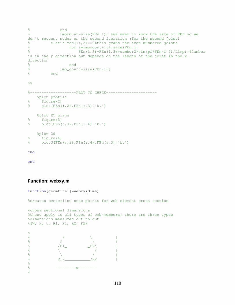
118
% end % impcount=size(FEn,1); %we need to kno w the size of FEn so we don't recount nodes on the second iteration (for th e second joist) % elseif mod(ii,2)==0%this grabs the even n umbered joists % for i=impcount+1:1:size(FEn,1) % FEn(i,3)=FEn(i,3)+camber2*sin (pi*FEn(i,2)/Limp);%Camber is in the y-direction but depends on the length of the joist in the x-direction % end % imp_count=size(FEn,1); % end %% %--------------------PLOT TO CHECK----------------- ----- %plot profile % figure(2) % plot(FEn(:,2),FEn(:,3),'k.') %plot ZY plane % figure(3) % plot(FEn(:,3),FEn(:,4),'k.') %plot 3d % figure(4) % plot3(FEn(:,2),FEn(:,4),FEn(:,3),'k.') end end
Function: webxy.m
function [geomfinal]=webxy(dims) %creates centerline node points for web element cro ss section %cross sectional dimensions %these apply to all types of web-members; there are three types %dimensions measured out-to-out %(W, H, t, R1, F1, R2, F2) % % / \ | % / \ | % /F1_ _F2\ H % \ / | % \ / | % R1\___________/R2 | % % ---------W-------- %

119
%section dimensions (total width (W), total height (H), thickness (t), %radius 1 (R1), radius 2 (R2) %Enter dims for practice % dims= [1 1 0.25 0.25 89 0.25 89]; W=dims(1); H=dims(2); t=dims(3); R1=dims(4); F1=dims(5)*pi/180; R2=dims(6); F2=dims(7)*pi/180; %origin is the intersection of the left "leg" and t he base %r=centerline radius r1=R1-t/2; r2=R2-t/2; %(x1,y1) represents the beginning of radius R1 x1=R1/tan(F1/2); y1=t/2; %(x2,y2) represents the beginning of radius R2 x2=W-R2/tan(F2/2); y2=t/2; %(x3,y3) represents the end of radius R1 %(xo3,yo3) represents the center of curvature of R1 xo3=x1; yo3=R1; G1=pi-F1; if G1<=pi/2 x3=xo3-r1*sin(G1); y3=yo3-r1*cos(G1); else x3=xo3-r1*cos(G1-pi/2); y3=yo3+r1*sin(G1-pi/2); end %(x4,y4) represents the end of radius R2 %(xo4,yo4) represents the center of curvature of R2 xo4=x2; yo4=R2; G2=pi-F2; if G2<=pi/2 x4=xo4+r2*sin(G2); y4=yo4-r2*cos(G2); else x4=xo4+r2*cos(G2-pi/2); y4=yo4+r2*sin(G2-pi/2);
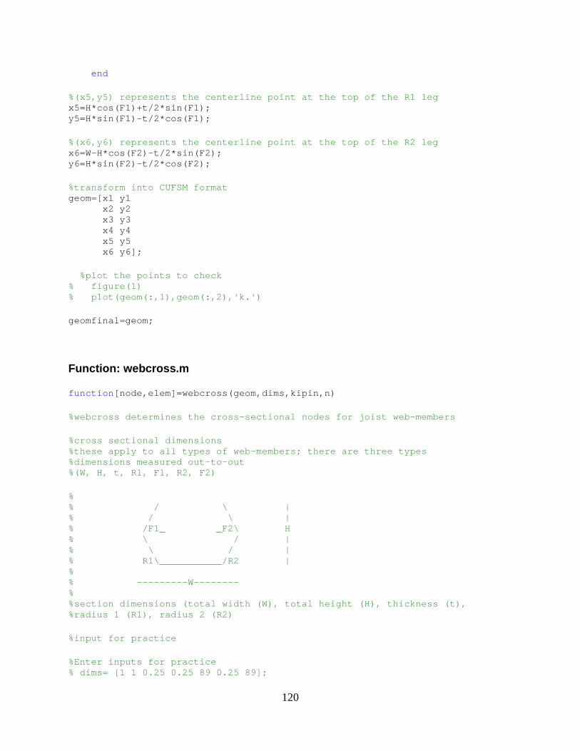
120
end %(x5,y5) represents the centerline point at the top of the R1 leg x5=H*cos(F1)+t/2*sin(F1); y5=H*sin(F1)-t/2*cos(F1); %(x6,y6) represents the centerline point at the top of the R2 leg x6=W-H*cos(F2)-t/2*sin(F2); y6=H*sin(F2)-t/2*cos(F2); %transform into CUFSM format geom=[x1 y1 x2 y2 x3 y3 x4 y4 x5 y5 x6 y6]; %plot the points to check % figure(1) % plot(geom(:,1),geom(:,2),'k.') geomfinal=geom;
Function: webcross.m
function [node,elem]=webcross(geom,dims,kipin,n) %webcross determines the cross-sectional nodes for joist web-members %cross sectional dimensions %these apply to all types of web-members; there are three types %dimensions measured out-to-out %(W, H, t, R1, F1, R2, F2) % % / \ | % / \ | % /F1_ _F2\ H % \ / | % \ / | % R1\___________/R2 | % % ---------W-------- % %section dimensions (total width (W), total height (H), thickness (t), %radius 1 (R1), radius 2 (R2) %input for practice %Enter inputs for practice % dims= [1 1 0.25 0.25 89 0.25 89];
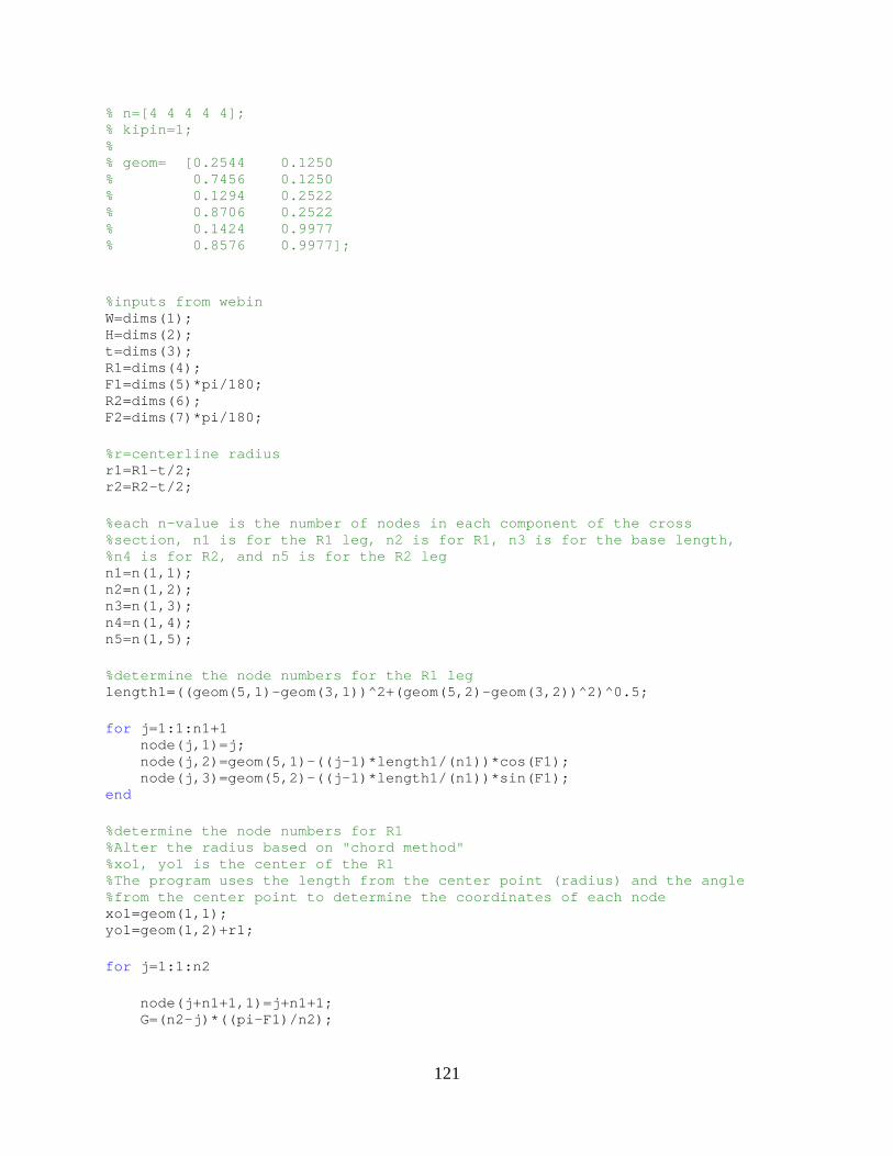
121
% n=[4 4 4 4 4]; % kipin=1; % % geom= [0.2544 0.1250 % 0.7456 0.1250 % 0.1294 0.2522 % 0.8706 0.2522 % 0.1424 0.9977 % 0.8576 0.9977]; %inputs from webin W=dims(1); H=dims(2); t=dims(3); R1=dims(4); F1=dims(5)*pi/180; R2=dims(6); F2=dims(7)*pi/180; %r=centerline radius r1=R1-t/2; r2=R2-t/2; %each n-value is the number of nodes in each compon ent of the cross %section, n1 is for the R1 leg, n2 is for R1, n3 is for the base length, %n4 is for R2, and n5 is for the R2 leg n1=n(1,1); n2=n(1,2); n3=n(1,3); n4=n(1,4); n5=n(1,5); %determine the node numbers for the R1 leg length1=((geom(5,1)-geom(3,1))^2+(geom(5,2)-geom(3, 2))^2)^0.5; for j=1:1:n1+1 node(j,1)=j; node(j,2)=geom(5,1)-((j-1)*length1/(n1))*cos(F1 ); node(j,3)=geom(5,2)-((j-1)*length1/(n1))*sin(F1 ); end %determine the node numbers for R1 %Alter the radius based on "chord method" %xo1, yo1 is the center of the R1 %The program uses the length from the center point (radius) and the angle %from the center point to determine the coordinates of each node xo1=geom(1,1); yo1=geom(1,2)+r1; for j=1:1:n2 node(j+n1+1,1)=j+n1+1; G=(n2-j)*((pi-F1)/n2);

122
if G<=pi/2 node(j+n1+1,2)=xo1-r1*sin(G); node(j+n1+1,3)=yo1-r1*cos(G); else node(j+n1+1,2)=xo1-r1*cos(G-pi/2); node(j+n1+1,3)=yo1+r1*sin(G-pi/2); end end %Determine the node numbers for the base of the web -member lengthb=geom(2,1)-geom(1,1); for j=1:1:n3 node(j+n1+n2+1,1)=j+n1+n2+1; node(j+n1+n2+1,2)=geom(1,1)+lengthb/(n3)*j; node(j+n1+n2+1,3)=geom(1,2); end %determine the node numbers for R2 %Alter the radius based on "chord method" %xo2, yo2 is the center of the R2 %The program uses the length from the center point (radius) and the angle %from the center point to determine the coordinates of each node xo2=geom(2,1); yo2=geom(2,2)+r2; for j=1:1:n4 node(j+n1+n2+n3+1,1)=j+n1+n2+n3+1; G=j*((pi-F2)/n4); if G<=pi/2 node(j+n1+n2+n3+1,2)=xo2+r2*sin(G); node(j+n1+n2+n3+1,3)=yo2-r2*cos(G); else node(j+n1+n2+n3+1,2)=xo2+r2*cos(G-pi/2); node(j+n1+n2+n3+1,3)=yo2+r2*sin(G-pi/2); end end %Determine the node numbers for the R2 leg length2=((geom(6,1)-geom(4,1))^2+(geom(6,2)-geom(4, 2))^2)^0.5; for j=1:1:n5 node(j+n1+n2+n3+n4+1,1)=j+n1+n2+n3+n4+1; node(j+n1+n2+n3+n4+1,2)=geom(4,1)-(j*length2/(n 5))*cos(F2); node(j+n1+n2+n3+n4+1,3)=geom(4,2)+(j*length2/(n 5))*sin(F2); end %check node to see if it is in the correct format %node
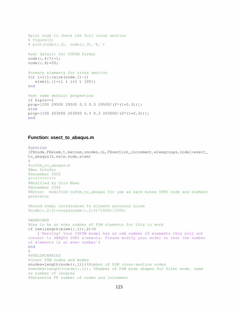
123
%plot node to check the full cross section % figure(2) % plot(node(:,2), node(:,3),'k.') %set default for CUFSM format node(:,4:7)=1; node(:,8)=50; %create elements for cross section for i=1:1:(size(node,1)-1) elem(i,:)=[i i i+1 t 100]; end %set some default properties if kipin==1 prop=[100 29500 29500 0.3 0.3 29500/(2*(1+0.3))]; else prop=[100 203000 203000 0.3 0.3 203000/(2*(1+0.3))] ; end
Function: xsect_to_abaqus.m
function [FEnode,FEelem,t,matnum,nnodes,nL,FEsection_increme nt,elemgroups,node]=xsect_to_abaqus(L,nele,node,elem) % %cufsm_to_abaqus.m %Ben Schafer %December 2005 %*********** %Modified by Cris Moen %November 2006 %Notes: modified cufsm_to_abaqus for use as bare b ones S9R5 node and element generator %Round nodal coordinates to elimate accuracy noise %node(:,2:3)=round(node(:,2:3)*1000)/1000; %WARNINGS %Has to be an even number of FSM elements for this to work if rem(length(elem(:,1)),2)>0 [ 'Warning! Your CUFSM model has an odd number of ele ments this will not convert to ABAQUS S9R5 elements. Please modify your model so that the number of elements is an even number' ] end % %PRELIMINARIES %Count FSM nodes and modes nnodes=length(node(:,1)); %Number of FSM cross-section nodes %nmodes=length(curve(:,1)); %Number of FSM mode sha pes for first mode, same as number of lengths %Determine FE number of nodes and increment

124
%Modify to a finer mesh: %original=nL=2*nele+1 nL=2*nele+1; %Number of FE nodes along the length %Determine the node numbering increment along the l ength if nnodes<100 FEsection_increment=100; %so along the length the numbering goes up by 100's else FEsection_increment=nnodes+1; end %NODAL COORDINATES IN FE FORM %FEnode=[node# x y z] x is along the length xincr=0; for i=1:nL FEnode((i-1)*nnodes+1:(i-1)*nnodes+nnodes,1)=node(:,1)+FEsection_increment*( i-1); %x in finite elements coordinate system FEnode((i-1)*nnodes+1:(i-1)*nnodes+nnodes,2)=xi ncr; %y in finite elements coordinate system FEnode((i-1)*nnodes+1:(i-1)*nnodes+nnodes,3)=no de(:,3); %z in finite elements coordinate system FEnode((i-1)*nnodes+1:(i-1)*nnodes+nnodes,4)=no de(:,2); xincr=xincr+L/(2*nele); end % %ELEMENT DEFINITIONS %Note, elements are done in strips, to reflect thic kness or material %changes which could exist in the FSM model. BUT! t he S9R5 element used %grabs the elements in pairs, so thickness or mater ial should be the same %for pairs of elements. %Note %Element Connectivity %ABAQUS S9R5 for example % face3 % 4--7--3 % | | %face4 8 9 6 face2 % | | % 1--5--2 % face1 %Go through the elements 2 at a time closedcross=1; if closedcross==1 k=1; %counter for strip, i.e., strip along the length (g roup of 2 FSM strips) step=1; for i=1:2:length(elem(:,1))-1 for j=1:(nL-1)/2 n1=elem(i,2); n2=elem(i+1,3); n3=elem(i+1,3) + 2*FEsection_increment; n4=elem(i,2) + 2*FEsection_increment; n5=elem(i,3);
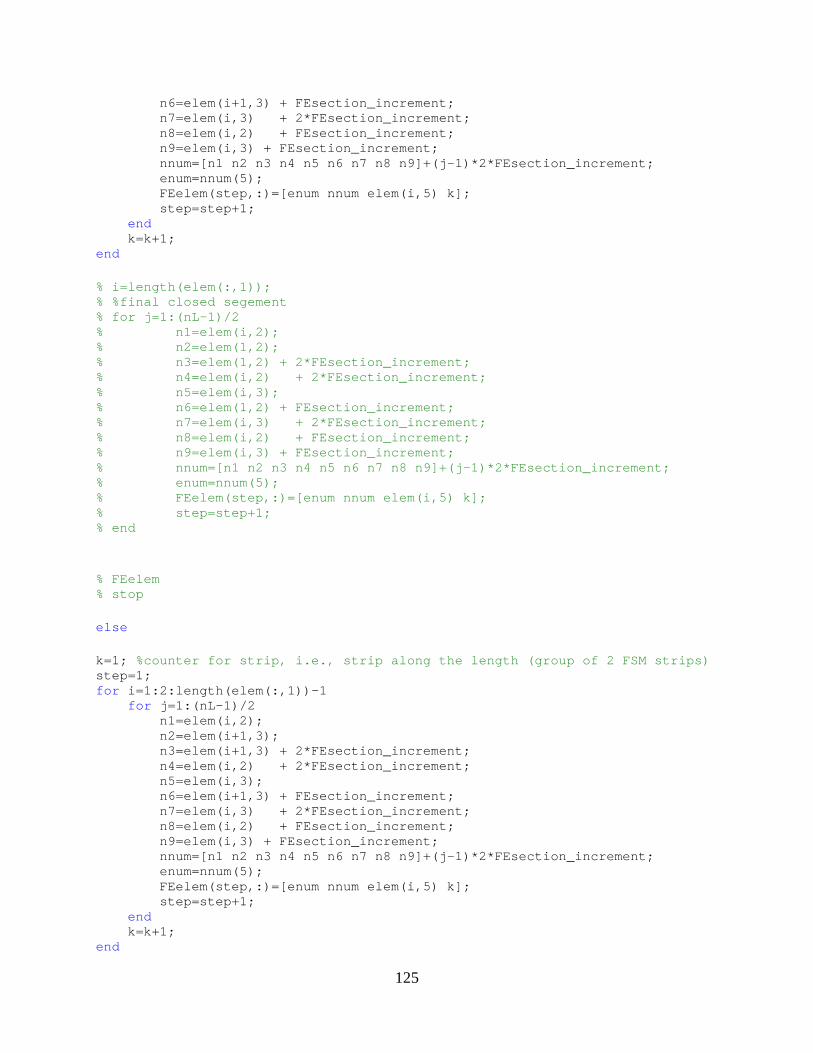
125
n6=elem(i+1,3) + FEsection_increment; n7=elem(i,3) + 2*FEsection_increment; n8=elem(i,2) + FEsection_increment; n9=elem(i,3) + FEsection_increment; nnum=[n1 n2 n3 n4 n5 n6 n7 n8 n9]+(j-1)*2*F Esection_increment; enum=nnum(5); FEelem(step,:)=[enum nnum elem(i,5) k]; step=step+1; end k=k+1; end % i=length(elem(:,1)); % %final closed segement % for j=1:(nL-1)/2 % n1=elem(i,2); % n2=elem(1,2); % n3=elem(1,2) + 2*FEsection_increment; % n4=elem(i,2) + 2*FEsection_increment; % n5=elem(i,3); % n6=elem(1,2) + FEsection_increment; % n7=elem(i,3) + 2*FEsection_increment; % n8=elem(i,2) + FEsection_increment; % n9=elem(i,3) + FEsection_increment; % nnum=[n1 n2 n3 n4 n5 n6 n7 n8 n9]+(j-1)*2 *FEsection_increment; % enum=nnum(5); % FEelem(step,:)=[enum nnum elem(i,5) k]; % step=step+1; % end % FEelem % stop else k=1; %counter for strip, i.e., strip along the length (g roup of 2 FSM strips) step=1; for i=1:2:length(elem(:,1))-1 for j=1:(nL-1)/2 n1=elem(i,2); n2=elem(i+1,3); n3=elem(i+1,3) + 2*FEsection_increment; n4=elem(i,2) + 2*FEsection_increment; n5=elem(i,3); n6=elem(i+1,3) + FEsection_increment; n7=elem(i,3) + 2*FEsection_increment; n8=elem(i,2) + FEsection_increment; n9=elem(i,3) + FEsection_increment; nnum=[n1 n2 n3 n4 n5 n6 n7 n8 n9]+(j-1)*2*F Esection_increment; enum=nnum(5); FEelem(step,:)=[enum nnum elem(i,5) k]; step=step+1; end k=k+1; end

126
end %ELEMENT THICKNESS AND MATERIAL NUMBER k=1; for i=1:2:length(elem(:,1))-1 t(k)=elem(i,4); matnum(k)=elem(i,5); k=k+1; end %ELEMENT GROUPS elemgroups=1:k-1;
Function: webassem.m
function [FEn,FEe,webcon,numdiag,numnodes,pinend] = webasse m(nodestack, elemstack, tstack, sectdims, TC, FIRST, depth, BC, FH, SEAT, Ltc, change,SPACE,GAP,H,N,FEn,FEe,ii,webcon,pinend) %This function determines the node and element numb ers for the web members %in the joist numnodes=3; %The number of nodes used for constraints of the we b members (5 nodes corresponds to the first two elements) %Change matrix values into their single values for easy use in this program depth=depth(ii,1)+change; TC=TC(ii,1); FIRST=FIRST(ii,1); BC=BC(ii,1); FH=FH(ii,1); SEAT=SEAT(ii,1); %Member 1: the outermost member in the joist %placement of each web member is based on the dista nce from the orgin of %the TOP CHORD % %Make two scenarios, one if we are on the first joi st, and another (when we %will have a node list already) for the remaining j oists if ii==1 %------Nodes for member 1----- nodes2=nodestack{2}; for i=1:size(nodes2,1) theta=abs(atan(depth/BC))+pi; %angle of web member length=(BC^2+depth^2)^.5; %length of the web member add=SEAT+SPACE; %additional x-value added to the web member FEn(i,1)=nodes2(i,1); %node numbers FEn(i,2:3)=nodes2(i,2:3)*[cos(theta) -sin(t heta); sin(theta) cos(theta)]; %Rotate x and y using matrix transformation FEn(i,2)=FEn(i,2)+add+abs(length*cos(theta) +2*abs(H(2)*sin(pi/2-theta))); %Move the x-coordinate to the correct location FEn(i,3)=FEn(i,3)-abs(length*sin(theta))+ch ange/2+abs(H(2)*cos(pi/2-theta)); %y coordinate FEn(i,4)=nodes2(i,4); %z coordinate
127
end %-----elements for member 1----- for i=1:size(elemstack{2},1) FEe(i,1)=i; FEe(i,2:10)=elemstack{2}(i,2:10); %Just add counter to FEe(i,2:10) because it relates the elements to the relative nod e numbers FEe(i,11)=elemstack{2}(i,11); FEe(i,12)=elemstack{2}(i,12); FEe(i,13)=tstack{2}(1,1); end %-----Make node list to use for constraints----- for k=1:4 %for the four welds on each web member if k==1 for j=1:numnodes constrain(j,:)=FEn(j,:); end for j=1:numnodes constrain(j+numnodes,:)=FEn((N+j),: ); end elseif k==2 for j=1:numnodes constrain(j,:)=FEn((N-numnodes+j),: ); end for j=1:numnodes constrain(j+numnodes,:)=FEn((N+N-nu mnodes+j),:); end elseif k==3 rowcount=size(nodestack{2},1); for j=1:numnodes constrain(j,:)=FEn(rowcount-N+j,:); end for j=1:numnodes constrain(j+numnodes,:)=FEn(rowcoun t-2*N+j,:); end else for j=1:numnodes constrain(j,:)=FEn(rowcount-numnode s+j,:); end for j=1:numnodes constrain(j+numnodes,:)=FEn(rowcoun t-numnodes-N+j,:); end end webcon{k}=constrain; end else %------Nodes for member 1----- nodes2=nodestack{2}; counter=size(FEn,1); counter2=100000000*(ii-1); for i=1:size(nodes2,1) theta=abs(atan(depth/BC))+pi; %angle of web member length=(BC^2+depth^2)^.5; %length of the web member add=SEAT+SPACE; %additional x-value added to the web member FEn(i+counter,1)=nodes2(i,1)+counter2; %node numbers
128
FEn(i+counter,2:3)=nodes2(i,2:3)*[cos(theta ) -sin(theta); sin(theta) cos(theta)]; %Rotate x and y using matrix transformation FEn(i+counter,2)=FEn(i+counter,2)+add+abs(length*co s(theta)+2*abs(H(2)*sin(pi/2-theta))); %Move the x-coordinate to the correct location FEn(i+counter,3)=FEn(i+counter,3)-abs(length*sin(theta))+change/2+abs(H(2)*cos(pi/2-t heta)); %y coordinate FEn(i+counter,4)=nodes2(i,4); %z coordinate end %-----elements for member 1----- ecount=size(FEe,1); enum=FEe(ecount,1); for i=1:size(elemstack{2},1) FEe(i+ecount,1)=i+enum; FEe(i+ecount,2:10)=elemstack{2}(i,2:10)+coun ter2; %Just add counter to FEe(i,2:10) because it relates the elements to the relative node numbers FEe(i+ecount,11)=elemstack{2}(i,11); FEe(i+ecount,12)=elemstack{2}(i,12); FEe(i+ecount,13)=tstack{2}(1,1); end %-----Make node list to use for constraints----- for k=1:4 if k==1 for j=1:numnodes constrain(j,:)=FEn(j+counter,:); end for j=1:numnodes constrain(j+numnodes,:)=FEn((N+j+co unter),:); end elseif k==2 for j=1:numnodes constrain(j,:)=FEn((N-numnodes+j+co unter),:); end for j=1:numnodes constrain(j+numnodes,:)=FEn((N+N-nu mnodes+j+counter),:); end elseif k==3 rowcount=size(nodestack{2},1); for j=1:numnodes constrain(j,:)=FEn(rowcount-N+j+cou nter,:); end for j=1:numnodes constrain(j+numnodes,:)=FEn(rowcoun t-2*N+j+counter,:); end else for j=1:numnodes constrain(j,:)=FEn(rowcount-numnode s+j+counter,:); end for j=1:numnodes constrain(j+numnodes,:)=FEn(rowcoun t-numnodes-N+j+counter,:); end end cols=size(webcon); kk=cols(1,2);
129
webcon{kk+1}=constrain; end end %plot profile to check % figure(2) % plot(FEn(:,2),FEn(:,3),'k.') %plot ZY plane % figure(3) % plot(FEn(:,3),FEn(:,4),'k.') %CHECK 3D % figure(3) % plot3(FEn(:,2),FEn(:,4),FEn(:,3),'k.') %Member 2: the 2nd outermost member in the joist %-----nodes for member 2----- nodes3=nodestack{3}; counter=size(FEn,1); counter2=100000+100000000*(ii-1); for i=1:size(nodes3,1) theta=pi+abs(atan(depth/(BC+SPACE-TC))); %angle of web member length=((BC+SPACE-TC)^2+depth^2)^.5; add=SEAT+TC; %additional x-value added to the web member FEn(i+counter,1)=nodes3(i,1)+counter2; %node numbers FEn(i+counter,2:3)=nodes3(i,2:3)*[cos(theta) -s in(theta); sin(theta) cos(theta)]; %Rotate x and y using matrix transformation FEn(i+counter,2)=FEn(i+counter,2)+abs(length*cos(th eta))+add+1/2*abs(H(3)*cos(pi/2-theta)); %Move the x-coordinate to the correct location FEn(i+counter,3)=FEn(i+counter,3)-abs(length*sin(theta))+change/2+1/2*abs(H(3)*sin(pi /2-theta)); %y-coordinate FEn(i+counter,4)=nodes3(i,4); %z coordinate end %-----elements for member 2----- ecount=size(FEe,1); enum=FEe(ecount,1); for i=1:size(elemstack{3},1) FEe(i+ecount,1)=(i+enum); FEe(i+ecount,2:10)=elemstack{3}(i,2:10)+counter2 ; %Just add counter to FEe(i,2:10) because it relates the elements to the relative node numbers FEe(i+ecount,11)=elemstack{3}(i,11); FEe(i+ecount,12)=elemstack{3}(i,12); FEe(i+ecount,13)=tstack{3}(1,1); end %-----Make node list to use for constraints----- for k=1:4 if k==1 for j=1:numnodes constrain(j,:)=FEn(j+counter,:);
130
end for j=1:numnodes constrain(j+numnodes,:)=FEn((N+j+co unter),:); end elseif k==2 for j=1:numnodes constrain(j,:)=FEn((N-numnodes+j+co unter),:); end for j=1:numnodes constrain(j+numnodes,:)=FEn((N+N-nu mnodes+j+counter),:); end elseif k==3 rowcount=size(nodestack{3},1); for j=1:numnodes constrain(j,:)=FEn(rowcount-N+j+cou nter,:); end for j=1:numnodes constrain(j+numnodes,:)=FEn(rowcoun t-2*N+j+counter,:); end else for j=1:numnodes constrain(j,:)=FEn(rowcount-numnode s+j+counter,:); end for j=1:numnodes constrain(j+numnodes,:)=FEn(rowcoun t-numnodes-N+j+counter,:); end end cols=size(webcon); kk=cols(1,2); webcon{kk+1}=constrain; end %plot profile to check % figure(2) % plot(FEn(:,2),FEn(:,3),'k.') %Member 3: the 3rd outermost member in the joist %-----nodes for member 3----- nodes4=nodestack{4}; counter=size(FEn,1); counter2=counter2+100000; for i=1:size(nodes4,1) theta=abs(atan(FH/depth))+pi/2; %angle of web member length=(depth^2+FH^2)^.5; add=SEAT+FIRST-SPACE; %additional x-value added to the web member FEn(i+counter,1)=nodes4(i,1)+counter2; %node numbers FEn(i+counter,2:3)=nodes4(i,2:3)*[cos(theta) -s in(theta); sin(theta) cos(theta)]; %Rotate x and y using matrix transformation FEn(i+counter,2)=FEn(i+counter,2)+add; %Move the x-coordinate to the correct location FEn(i+counter,3)=FEn(i+counter,3)-change/2; %y coordinate FEn(i+counter,4)=nodes4(i,4); %z coordinate end %-----elements for member 3----- ecount=size(FEe,1);

131
enum=FEe(ecount,1); for i=1:size(elemstack{4},1) FEe(i+ecount,1)=(i+enum); FEe(i+ecount,2:10)=elemstack{4}(i,2:10)+counter2 ; %within element FEe(i+ecount,11)=elemstack{4}(i,11); FEe(i+ecount,12)=elemstack{4}(i,12); FEe(i+ecount,13)=tstack{4}(1,1); end %-----Make node list to use for constraints----- for k=1:4 if k==1 for j=1:numnodes constrain(j,:)=FEn(j+counter,:); end for j=1:numnodes constrain(j+numnodes,:)=FEn((N+j+co unter),:); end elseif k==2 for j=1:numnodes constrain(j,:)=FEn((N-numnodes+j+co unter),:); end for j=1:numnodes constrain(j+numnodes,:)=FEn((N+N-nu mnodes+j+counter),:); end elseif k==3 rowcount=size(nodestack{4},1); for j=1:numnodes constrain(j,:)=FEn(rowcount-N+j+cou nter,:); end for j=1:numnodes constrain(j+numnodes,:)=FEn(rowcoun t-2*N+j+counter,:); end else for j=1:numnodes constrain(j,:)=FEn(rowcount-numnode s+j+counter,:); end for j=1:numnodes constrain(j+numnodes,:)=FEn(rowcoun t-numnodes-N+j+counter,:); end end cols=size(webcon); kk=cols(1,2); webcon{kk+1}=constrain; end %plot profile to check % figure(2) % plot(FEn(:,2),FEn(:,3),'k.') %Member 5: the 45 degree pieces of the joist -- and additional web members %in this same orientation numdiag=round(((Ltc-2*SEAT-2*FIRST)/(depth))*1/2); %the number of diagonals in the joist (for each 45 degree orientation)

132
%this may need to change, this is not exact and my not be applicable to all %joists %-----nodes for these members----- nodes1=nodestack{1}; counter=size(FEn,1); counter2=counter2+100000; %Before node for j=1:numdiag for i=1:size(nodes1,1) theta=pi/2+atan(1); %angle of web member length=sqrt(2*depth^2); add=SEAT+FIRST+(depth+GAP)*2+2*(depth+GAP)* (j-1); %additional x-value added to the web member FEn(i+counter,1)=nodes1(i,1)+counter2; %within node FEn(i+counter,2:3)=nodes1(i,2:3)*[cos(theta ) -sin(theta); sin(theta) cos(theta)]; %Rotate x and y using matrix transformation FEn(i+counter,2)=FEn(i+counter,2)+add; %Move the x-coordinate to the correct location FEn(i+counter,3)=FEn(i+counter,3)-change/2; %y coordinate FEn(i+counter,4)=nodes1(i,4); %z coordinate end %plot profile to check % figure(2) % plot(FEn(:,2),FEn(:,3),'k.') %-----elements for these members----- ecount=size(FEe,1); enum=FEe(ecount,1); for i=1:size(elemstack{1},1) FEe(i+ecount,1)=(i+enum); FEe(i+ecount,2:10)=elemstack{1}(i,2:10)+ counter2; %within element FEe(i+ecount,11)=elemstack{1}(i,11); FEe(i+ecount,12)=elemstack{1}(i,12); FEe(i+ecount,13)=tstack{1}(1,1); end counter2=counter2+100000; %Before node %-----Make node list to use for constraints----- for k=1:4 if k==1 for j=1:numnodes constrain(j,:)=FEn(j+counter,:); end for j=1:numnodes constrain(j+numnodes,:)=FEn((N+j+co unter),:); end elseif k==2 for j=1:numnodes constrain(j,:)=FEn((N-numnodes+j+co unter),:); end for j=1:numnodes constrain(j+numnodes,:)=FEn((N+N-nu mnodes+j+counter),:); end elseif k==3
133
rowcount=size(nodestack{1},1); for j=1:numnodes constrain(j,:)=FEn(rowcount-2*N+j+c ounter,:); end for j=1:numnodes constrain(j+numnodes,:)=FEn(rowcoun t-3*N+j+counter,:); end else for j=1:numnodes constrain(j,:)=FEn(rowcount-numnode s-N+j+counter,:); end for j=1:numnodes constrain(j+numnodes,:)=FEn(rowcoun t-numnodes-2*N+j+counter,:); end end cols=size(webcon); kk=cols(1,2); webcon{kk+1}=constrain; end counter=size(FEn,1); %Change counter for the next iteration end %plot profile to check % figure(2) % plot(FEn(:,2),FEn(:,3),'k.') %Member 6: the 45 degree pieces of the joist (facin g the opposite way) nodes1=nodestack{1}; counter=size(FEn,1); counter2=counter2+100000; %Before node for j=1:numdiag for i=1:size(nodes1,1) theta=pi+atan(1); %angle of web member length=sqrt(2*depth^2); add=SEAT+FIRST+2*(depth+GAP)*(j-1); %additional x-value added to the web member FEn(i+counter,1)=nodes1(i,1)+counter2; %within node FEn(i+counter,2:3)=nodes1(i,2:3)*[cos(theta ) -sin(theta); sin(theta) cos(theta)]; %Rotate x and y using matrix transformation FEn(i+counter,2)=FEn(i+counter,2)+abs(length*cos(th eta))+add+H(1)*0.707; %Move the x-coordinate to the correct location FEn(i+counter,3)=FEn(i+counter,3)-abs(lengt h*sin(theta))+change; FEn(i+counter,4)=nodes1(i,4); %z coordinate end % %plot profile to check % figure(2) % plot(FEn(:,2),FEn(:,3),'k.') %-----elements for these members-----
134
ecount=size(FEe,1); enum=FEe(ecount,1); for i=1:size(elemstack{1},1) FEe(i+ecount,1)=(i+enum); FEe(i+ecount,2:10)=elemstack{1}(i,2:10)+ counter2; %within element FEe(i+ecount,11)=elemstack{1}(i,11); FEe(i+ecount,12)=elemstack{1}(i,12); FEe(i+ecount,13)=tstack{1}(1,1); end counter2=counter2+100000; %Before node %-----Make node list to use for constraints----- for k=1:4 if k==1 for j=1:numnodes constrain(j,:)=FEn(j+counter,:); end for j=1:numnodes constrain(j+numnodes,:)=FEn((N+j+co unter),:); end elseif k==2 for j=1:numnodes constrain(j,:)=FEn((N-numnodes+j+co unter),:); end for j=1:numnodes constrain(j+numnodes,:)=FEn((N+N-nu mnodes+j+counter),:); end elseif k==3 rowcount=size(nodestack{1},1); for j=1:numnodes constrain(j,:)=FEn(rowcount-2*N+j+c ounter,:); end for j=1:numnodes constrain(j+numnodes,:)=FEn(rowcoun t-3*N+j+counter,:); end else for j=1:numnodes constrain(j,:)=FEn(rowcount-numnode s-N+j+counter,:); end for j=1:numnodes constrain(j+numnodes,:)=FEn(rowcoun t-numnodes-2*N+j+counter,:); end end cols=size(webcon); kk=cols(1,2); webcon{kk+1}=constrain; end counter=size(FEn,1); end %plot profile to check % figure(2) % plot(FEn(:,2),FEn(:,3),'k.')
135
%additional amount to be taken out of joist sub=numdiag*GAP; %Member 8: the 3rd outermost member in the joist on the far side nodes4=nodestack{4}; counter=size(FEn,1); counter2=counter2+100000; %Before node for i=1:size(nodes4,1) theta=pi+abs(atan(depth/FH)); %angle of web member length=sqrt(depth^2+FH^2); add=Ltc-SEAT-FIRST-sub+2*SPACE; %additional x-value added to the web member FEn(i+counter,1)=nodes4(i,1)+counter2; %within node FEn(i+counter,2:3)=nodes4(i,2:3)*[cos(theta) -s in(theta); sin(theta) cos(theta)]; %Rotate x and y using matrix transformation FEn(i+counter,2)=FEn(i+counter,2)+abs(length*co s(theta))+add; %Move the x-coordinate to the correct location FEn(i+counter,3)=FEn(i+counter,3)-abs(length*si n(theta))+change/2; FEn(i+counter,4)=nodes4(i,4); %z coordinate end %-----elements for this member----- ecount=size(FEe,1); enum=FEe(ecount,1); for i=1:size(elemstack{4},1) FEe(i+ecount,1)=(i+enum); FEe(i+ecount,2:10)=elemstack{4}(i,2:10)+counter2 ; %within element FEe(i+ecount,11)=elemstack{4}(i,11); FEe(i+ecount,12)=elemstack{4}(i,12); FEe(i+ecount,13)=tstack{4}(1,1); end %-----Make node list to use for constraints----- for k=1:4 if k==1 for j=1:numnodes constrain(j,:)=FEn(j+counter,:); end for j=1:numnodes constrain(j+numnodes,:)=FEn((N+j+co unter),:); end elseif k==2 for j=1:numnodes constrain(j,:)=FEn((N-numnodes+j+co unter),:); end for j=1:numnodes constrain(j+numnodes,:)=FEn((N+N-nu mnodes+j+counter),:); end elseif k==3 rowcount=size(nodestack{4},1); for j=1:numnodes constrain(j,:)=FEn(rowcount-N+j+cou nter,:); end for j=1:numnodes
136
constrain(j+numnodes,:)=FEn(rowcoun t-2*N+j+counter,:); end else for j=1:numnodes constrain(j,:)=FEn(rowcount-numnode s+j+counter,:); end for j=1:numnodes constrain(j+numnodes,:)=FEn(rowcoun t-numnodes-N+j+counter,:); end end cols=size(webcon); kk=cols(1,2); webcon{kk+1}=constrain; end %plot profile to check % figure(2) % plot(FEn(:,2),FEn(:,3),'k.') %Member 9: the 2nd outermost member in the joist on the far side %-----nodes for this member----- nodes3=nodestack{3}; counter=size(FEn,1); counter2=counter2+100000; %Before node for i=1:size(nodes3,1) theta=pi/2+abs(atan((BC+SPACE-TC)/depth)); %angle of web member length=sqrt((BC+SPACE-TC)^2+depth^2); add=Ltc-SEAT-TC-sub; %additional x-value added to the web member FEn(i+counter,1)=nodes3(i,1)+counter2; %within node FEn(i+counter,2:3)=nodes3(i,2:3)*[cos(theta) -s in(theta); sin(theta) cos(theta)]; %Rotate x and y using matrix transformation FEn(i+counter,2)=FEn(i+counter,2)+add+1/2*abs(H (3)*cos(pi/2-theta)); %Move the x-coordinate to the correct location FEn(i+counter,3)=FEn(i+counter,3)-change/2+1/2* abs(H(3)*sin(pi/2-theta)); %y coordinate FEn(i+counter,4)=nodes3(i,4); %z coordinate end %-----elements for this member----- ecount=size(FEe,1); enum=FEe(ecount,1); for i=1:size(elemstack{3},1) FEe(i+ecount,1)=(i+enum); FEe(i+ecount,2:10)=elemstack{3}(i,2:10)+counter2 ; %within element FEe(i+ecount,11)=elemstack{3}(i,11); FEe(i+ecount,12)=elemstack{3}(i,12); FEe(i+ecount,13)=tstack{3}(1,1); end %-----Make node list to use for constraints----- for k=1:4 if k==1 for j=1:numnodes constrain(j,:)=FEn(j+counter,:); end

137
for j=1:numnodes constrain(j+numnodes,:)=FEn((N+j+co unter),:); end elseif k==2 for j=1:numnodes constrain(j,:)=FEn((N-numnodes+j+co unter),:); end for j=1:numnodes constrain(j+numnodes,:)=FEn((N+N-nu mnodes+j+counter),:); end elseif k==3 rowcount=size(nodestack{3},1); for j=1:numnodes constrain(j,:)=FEn(rowcount-N+j+cou nter,:); end for j=1:numnodes constrain(j+numnodes,:)=FEn(rowcoun t-2*N+j+counter,:); end else for j=1:numnodes constrain(j,:)=FEn(rowcount-numnode s+j+counter,:); end for j=1:numnodes constrain(j+numnodes,:)=FEn(rowcoun t-numnodes-N+j+counter,:); end end cols=size(webcon); kk=cols(1,2); webcon{kk+1}=constrain; end %plot profile to check % figure(2) % plot(FEn(:,2),FEn(:,3),'k.') %Member 10: the 1st outermost member in the joist o n the far side %-----nodes for this member----- nodes2=nodestack{2}; counter=size(FEn,1); counter2=counter2+100000; %Before node for i=1:size(nodes2,1) theta=pi/2+abs(atan(BC/depth)); %angle of web member length=sqrt(depth^2+BC^2); add=Ltc-SEAT-sub; %additional x-value added to the web member FEn(i+counter,1)=nodes2(i,1)+counter2; %within node FEn(i+counter,2:3)=nodes2(i,2:3)*[cos(theta) -s in(theta); sin(theta) cos(theta)]; %Rotate x and y using matrix transformation FEn(i+counter,2)=FEn(i+counter,2)+add+abs(H(2)* cos(pi/2-theta)); %Move the x-coordinate to the correct location FEn(i+counter,3)=FEn(i+counter,3); %y coordinate FEn(i+counter,4)=nodes2(i,4); %z coordinate end %

138
%-----elements for this member----- ecount=size(FEe,1); enum=FEe(ecount,1); for i=1:size(elemstack{2},1) FEe(i+ecount,1)=(i+enum); FEe(i+ecount,2:10)=elemstack{2}(i,2:10)+counter2 ; %within element FEe(i+ecount,11)=elemstack{2}(i,11); FEe(i+ecount,12)=elemstack{2}(i,12); FEe(i+ecount,13)=tstack{2}(1,1); end %-----Make node list to use for constraints----- for k=1:4 if k==1 for j=1:numnodes constrain(j,:)=FEn(j+counter,:); end for j=1:numnodes constrain(j+numnodes,:)=FEn((N+j+co unter),:); end elseif k==2 for j=1:numnodes constrain(j,:)=FEn((N-numnodes+j+co unter),:); end for j=1:numnodes constrain(j+numnodes,:)=FEn((N+N-nu mnodes+j+counter),:); end elseif k==3 rowcount=size(nodestack{2},1); for j=1:numnodes constrain(j,:)=FEn(rowcount-N+j+cou nter,:); end for j=1:numnodes constrain(j+numnodes,:)=FEn(rowcoun t-2*N+j+counter,:); end else for j=1:numnodes constrain(j,:)=FEn(rowcount-numnode s+j+counter,:); end for j=1:numnodes constrain(j+numnodes,:)=FEn(rowcoun t-numnodes-N+j+counter,:); end end cols=size(webcon); kk=cols(1,2); webcon{kk+1}=constrain; end %plot profile to check % figure(2) % plot(FEn(:,2),FEn(:,3),'k.') %Member 11: the VERTICAL pieces on the first 1/2 of the joist %-----NODES for these members-----
139
numvert=round(numdiag*1/2); %number of vertical web members per 1/2 span (it is equal to half of the number if diagonal members) nodes5=nodestack{5}; for j=1:numvert counter=size(FEn,1); counter2=counter2+100000; %Before node for i=1:size(nodes5,1) theta=pi/2; %angle of web member add=SEAT+FIRST+GAP+depth+2*(depth+G AP)*(j-1)+H(5)/2; %additional x-value added to the web member FEn(i+counter,1)=nodes5(i,1)+counte r2; %within node FEn(i+counter,2:3)=nodes5(i,2:3)*[c os(theta) -sin(theta); sin(theta) cos(theta)]; %Rotate x and y using matrix transformation FEn(i+counter,2)=FEn(i+counter,2)+a dd; %Move the x-coordinate to the correct location FEn(i+counter,3)=FEn(i+counter,3); %y coordinate FEn(i+counter,4)=nodes5(i,4); %z coordinate end %-----elements for this member----- ecount=size(FEe,1); enum=FEe(ecount,1); for i=1:size(elemstack{5},1) FEe(i+ecount,1)=(i+enum); FEe(i+ecount,2:10)=elemstack{5}(i,2:10)+ counter2; %within element FEe(i+ecount,11)=elemstack{5}(i,11); FEe(i+ecount,12)=elemstack{5}(i,12); FEe(i+ecount,13)=tstack{5}(1,1); end %-----Make node list to use for constraints----- for k=1:4 if k==1 for j=1:numnodes constrain(j,:)=FEn(j+counter,:); end for j=1:numnodes constrain(j+numnodes,:)=FEn((N+j+co unter),:); end elseif k==2 for j=1:numnodes constrain(j,:)=FEn((N-numnodes+j+co unter),:); end for j=1:numnodes constrain(j+numnodes,:)=FEn((N+N-nu mnodes+j+counter),:); end elseif k==3 rowcount=size(nodestack{5},1); for j=1:numnodes constrain(j,:)=FEn(rowcount-N+j+cou nter,:); end for j=1:numnodes constrain(j+numnodes,:)=FEn(rowcoun t-2*N+j+counter,:); end else
140
for j=1:numnodes constrain(j,:)=FEn(rowcount-numnode s+j+counter,:); end for j=1:numnodes constrain(j+numnodes,:)=FEn(rowcoun t-numnodes-N+j+counter,:); end end cols=size(webcon); kk=cols(1,2); webcon{kk+1}=constrain; end %plot profile to check % figure(2) % plot(FEn(:,2),FEn(:,3),'k.') end %Member 12: the vertical pieces on the second 1/2 o f the joist %-----NODES for these members----- nodes5=nodestack{5}; %Determine if there is an odd or even number of ver tical pieces for placement if mod(numdiag,2)==0 numvert=numvert; addvert=numvert; else addvert=numvert; numvert=numvert-1; end for j=1:numvert %this may need to change if there is an uneven amou nt of vertical pieces counter=size(FEn,1); counter2=counter2+100000; %Before node for i=1:size(nodes5,1) theta=3*pi/2; %angle of web member add=SEAT+FIRST+2*GAP+SPACE+depth+2*addvert*(GAP+dep th)+2*(GAP+depth)*(j-1)-H(5)/2; %additional x-value added to the web member FEn(i+counter,1)=nodes5(i,1)+counte r2; %within node FEn(i+counter,2:3)=nodes5(i,2:3)*[c os(theta) -sin(theta); sin(theta) cos(theta)]; %Rotate x and y using matrix transformation FEn(i+counter,2)=FEn(i+counter,2)+a dd+H(5)*3/4; %Move the x-coordinate to the correct location FEn(i+counter,3)=FEn(i+counter,3)-d epth; FEn(i+counter,4)=nodes5(i,4); %z coordinate end %-----elements for this member----- ecount=size(FEe,1); enum=FEe(ecount,1); for i=1:size(elemstack{5},1) FEe(i+ecount,1)=(i+enum);

141
FEe(i+ecount,2:10)=elemstack{5}(i,2:10)+ counter2; %within element FEe(i+ecount,11)=elemstack{5}(i,11); FEe(i+ecount,12)=elemstack{5}(i,12); FEe(i+ecount,13)=tstack{5}(1,1); end %-----Make node list to use for constraints----- for k=1:4 if k==1 for j=1:numnodes constrain(j,:)=FEn(j+counter,:); end for j=1:numnodes constrain(j+numnodes,:)=FEn((N+j+co unter),:); end elseif k==2 for j=1:numnodes constrain(j,:)=FEn((N-numnodes+j+co unter),:); end for j=1:numnodes constrain(j+numnodes,:)=FEn((N+N-nu mnodes+j+counter),:); end elseif k==3 rowcount=size(nodestack{5},1); for j=1:numnodes constrain(j,:)=FEn(rowcount-N+j+cou nter,:); end for j=1:numnodes constrain(j+numnodes,:)=FEn(rowcoun t-2*N+j+counter,:); end else for j=1:numnodes constrain(j,:)=FEn(rowcount-numnode s+j+counter,:); end for j=1:numnodes constrain(j+numnodes,:)=FEn(rowcoun t-numnodes-N+j+counter,:); end end cols=size(webcon); kk=cols(1,2); webcon{kk+1}=constrain; end %plot profile to check % figure(2) % plot(FEn(:,2),FEn(:,3),'k.') end %-----------------Plot to check---------------- %plot profile % figure(2) % plot(FEn(:,2),FEn(:,3),'k.') %plot 3D to see extrusion along the length of the m ember % figure(1) % plot3(FEn(:,2),FEn(:,4),FEn(:,3),'k.')
142
%For the pinned boundary condition at the far end, determine where the seat %should start if ii==1 %Only for the first iteration, because if after tha t FEn contains all the nodes from the first joist including the ch ord members which will extend past this point pinend=max(FEn(:,2)); %Maximum x-coordinate end end
Function: SPACERassem.m
function [FEn,FEe,TCbatpos,BCbatpos,numbattens]=SPACERassem( nodestack,FEn,FIRST,SEAT,depth,GAP,FEe,elemstack,tstack,Ltc,webcon,N,H,numdia g,ii) %Add the nodes and elements for the bottom chord in to the GLOBAL node and %element matrices numnodes=5; %The number of nodes used for the spacer constraint s %The number of spacers changes based on the design of each joist. The %following is a general equation that inserts batte ns in the same manner as %the 24K4 joists, it should be changed for designs that use a different %algorithm for battens numbattens=2*(numdiag-4); %the number of spacers for the TC ONLY!!!!! %spacer members %-----NODES FOR THE CHORD MEMBERS----- batten1=nodestack{1}; %We need to swap the x and z coordinates of the spa cer to account for its %orientation holder(:,1)=batten1(:,2); batten1(:,2)=batten1(:,4); batten1(:,4)=holder(:,1); for j=1:numbattens for i=1:size(batten1,1) MPCbat(i,1)=batten1(i,1); MPCbat(i,2)=batten1(i,2)+FIRST(ii)+SEAT(ii)+depth(i i)*4.5+6*GAP+(depth(ii)+GAP)*(j-1)+1; %x coordinate MPCbat(i,3)=batten1(i,3); %y coordinate MPCbat(i,4)=batten1(i,4); %z coordinate plus the gap in between the chord end TCbatpos{j}=MPCbat; end %-----SPACERS IN THE BC----- for j=1:1 %For this design there is only one spacer in the BC
143
for i=1:size(batten1,1) MPCbat(i,1)=batten1(i,1); %within node MPCbat(i,2)=batten1(i,2)+Ltc/2+2*(depth(ii) +GAP)*(j-1); %x coordinate MPCbat(i,3)=batten1(i,3)-depth(ii)+H; %y coordinate MPCbat(i,4)=batten1(i,4); %z coordinate plus the gap in between the chord end BCbatpos{j}=MPCbat; end %OLD STUFF USING *FASTENER (DIDN'T WORK) THAT IS GO OD TO KEEP JUST IN CASE: %-----SPACERS IN THE TC----- %The following was from using fasteners % for j=1:numbattens % counter=size(FEn,1); % counter2=100000000+1000000*j; %Before node % for i=1:size(batten1,1) % FEn(i+counter,1)=batten1(i,1)+counter2; %within node % FEn(i+counter,2)=batten1(i,2)+FIRST+SEAT+depth*4.5+ 6*GAP+(depth+GAP)*(j-1); %x coordinate % FEn(i+counter,3)=batten1(i,3); %y coordi nate % FEn(i+counter,4)=batten1(i,4); %z coordin ate plus the gap in between the chord % end %Plot battens to check % figure(7) % plot(FEn(:,2),FEn(:,3),'k.') %CHECK 3D % figure(3) % plot3(FEn(:,2),FEn(:,4),FEn(:,3),'k.') %NODE LIST USED FOR CONSTRAINTS FOR *FASTENER %-----Make node list to use for constraints----- % for k=1:4 % if k==1 % for l=1:numnodes % constrain(l,:)=FEn(l+counter,:); % end % % for l=1:numnodes % % constrain(l+numnodes,:)=FEn((N+ l+counter),:); % % end % elseif k==2 % for l=1:numnodes % constrain(l,:)=FEn((N-numnodes+l+ counter),:); % end % % for l=1:numnodes
144
% % constrain(l+numnodes,:)=FEn((N+ N-numnodes+l+counter+1),:); % % end % elseif k==3 % rowcount=size(batten1,1); %CHANGE % for l=1:numnodes % constrain(l,:)=FEn(rowcount-N+l+c ounter+1,:); % end % % for l=1:numnodes % % constrain(l+numnodes,:)=FEn(row count-2*N+l+counter,:); % % end % else % for l=1:numnodes % constrain(l,:)=FEn(rowcount-numno des+l+counter,:); % end % % for l=1:numnodes % % constrain(l+numnodes,:)=FEn(row count-numnodes-N+l+counter-1,:); % % end % end % xbc=size(webcon); % next=xbc(1,2); % webcon{next+1}=constrain; % end %Elements used for this chord for *fastener %-----elements for this chord----- % ecount=size(FEe,1); % enum=FEe(ecount,1); % for i=1:size(elemstack{1},1) % FEe(i+ecount,1)=(i+enum); % FEe(i+ecount,2:10)=elemstack{1}(i,2:10)+co unter2; %within element % FEe(i+ecount,11)=elemstack{1}(i,11); % FEe(i+ecount,12)=elemstack{1}(i,12); % FEe(i+ecount,13)=tstack{1}(1,1); % end % % end % %-----SPACERS IN THE BC----- % for j=1:1 %For this design there is only one spa cer in the BC % counter=size(MPCbat,1); % counter2=2000000*j; %Before node % for i=1:size(batten1,1) % FEn(i+counter,1)=batten1(i,1)+counter2; %within node % FEn(i+counter,2)=batten1(i,2)+Ltc/2+2*(de pth+GAP)*(j-1); %x coordinate % FEn(i+counter,3)=batten1(i,3)-depth+H; % y coordinate % FEn(i+counter,4)=batten1(i,4); %z coordin ate plus the gap in between the chord % end % % %Plot spacers to check % % figure(7)
145
% % plot(FEn(:,2),FEn(:,3),'k.') % % %CHECK 3D % % figure(3) % % plot3(FEn(:,2),FEn(:,4),FEn(:,3),'k.') % % %-----Make node list to use for constraints-- --- % for k=1:4 % if k==1 % for l=1:numnodes % constrain(l,:)=FEn(l+counter,:); % end % % for l=1:numnodes % % constrain(l+numnodes,:)=FEn((N+ l+counter-1),:); % % end % elseif k==2 % for l=1:numnodes % constrain(l,:)=FEn((N-numnodes+l+ counter),:); % end % % for l=1:numnodes % % constrain(l+numnodes,:)=FEn((N+ N-numnodes+l+counter-1),:); % % end % elseif k==3 % rowcount=size(batten1,1); %CHANGE % for l=1:numnodes % constrain(l,:)=FEn(rowcount-N+l+c ounter+1,:); % end % % for l=1:numnodes % % constrain(l+numnodes,:)=FEn(row count-2*N+l+counter-1,:); % % end % else % for l=1:numnodes % constrain(l,:)=FEn(rowcount-numno des+l+counter,:); % end % % for l=1:numnodes % % constrain(l+numnodes,:)=FEn(row count-numnodes-N+l+counter-1,:); % % end % end % xbc=size(webcon); % next=xbc(1,2); % webcon{next+1}=constrain; % end % % % %-----elements for this chord----- % ecount=size(FEe,1); % enum=FEe(ecount,1); % for i=1:size(elemstack{1},1) % FEe(i+ecount,1)=(i+enum); % FEe(i+ecount,2:10)=elemstack{1}(i,2:10)+co unter2; %within element % FEe(i+ecount,11)=elemstack{1}(i,11); % FEe(i+ecount,12)=elemstack{1}(i,12); % FEe(i+ecount,13)=tstack{1}(1,1); % end %
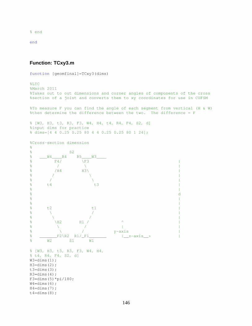
146
% end end
Function: TCxy3.m
function [geomfinal]=TCxy3(dims) %LTC %March 2011 %Takes out to out dimensions and corner angles of c omponents of the cross %section of a joist and converts them to xy coordin ates for use in CUFSM %To measure F you can find the angle of each segmen t from vertical (H & W) %then determine the difference between the two. Th e difference = F % [W3, H3, t3, R3, F3, W4, H4, t4, R4, F4, S2, d] %input dims for practice % dims=[4 4 0.25 0.25 80 4 4 0.25 0.25 80 1 24]; %Cross-section dimension % % S2 % ___W4____R4 R5____W3____ % F4/ \F3 | % / \ | % /H4 H3\ | % / \ | % / \ | % t4 t3 | % | % d % | % | % t2 t1 | % \ / | % \ / | % \H2 H1 / ^ | % \ / | | % \ / y-axis | % _______F2\R2 R1/_F1_______ |__z-axis__> | % W2 S1 W1 % [W3, H3, t3, R3, F3, W4, H4, % t4, R4, F4, S2, d] W3=dims(1); H3=dims(2); t3=dims(3); R3=dims(4); F3=dims(5)*pi/180; W4=dims(6); H4=dims(7); t4=dims(8);
147
R4=dims(9); F4=dims(10)*pi/180; S2=dims(11); d=dims(12); %orgin is intersection of H1-line and W1-line %r=the centerline radius of the angle r3=R3-t3/2; %(x9,y9) represents the beginning of the radius of the W-3 leg xx3=0; yy3=d; x9=R3/tan(F3/2); y9=yy3-t3/2; %(xc3, yc3) represents the center of the arc 3 xc3=x9; yc3=y9-r3; %(x10,y10) represents the beginning of the radius o n the H3-leg G3=pi-F3; if G3<=pi/2 x10=xc3-r3*sin(G3); y10=yc3+r3*cos(G3); else x10=xc3-r3*cos(G3-pi/2); y10=yc3-r3*sin(G3-pi/2); end %(x11,y11) represents the centerline point at the e nd of length W3 x11=xx3+W3; y11=yy3-t3/2; %(x12,y12) represents the centerline point at the e nd of length H3 x12=xx3+H3*cos(F3)+t3/2*sin(F3); y12=yy3-H3*sin(F3)+t3/2*cos(F3); %transform into CUFSM format geom=[ x9 y9 x10 y10 x11 y11 x12 y12]; %plot the points to check % figure(1) % plot(geom(:,1),geom(:,2),'k.'); geomfinal=geom;

148
Function: TCcross3.m
function [node,elem]=TCcross(geom,dims,kipin, n) %geom gives the xy-coordinates of each of the four nodes previously defined %DETERMINES THE NODE NUMBERS FOR THE TOP CHORD (angles "3" and "4") % [W3, H3, t3, R3, F3, W4, H4, t4, R4, F4, S2, d] %Cross-section dimensions % % S2 % ___W4____R4 R5____W3____ % F4/ \F3 | % / \ | % /H4 H3\ | % / \ | % / \ | % t4 t3 | % | % d % | % | % t2 t1 | % \ / | % \ / | % \H2 H1 / ^ | % \ / | | % \ / y-axis | % _______F2\R2 R1/_F1_______ |__x-axis__> | % W2 S1 W1 %input dims for practice % dims=[4 4 0.25 0.25 80 4 4 0.25 0.25 80 1 24]; % n=[4 4 4]; % geom =[0.2979 23.8750 % 0.1748 23.7283 % 4.0000 23.8750 % 0.8177 20.0825 % -1.2979 23.8750 % -1.1748 23.7283 % -5.0000 23.8750 % -1.8177 20.0825]; % kipin=1; % %input section dimensions from chordin W3=dims(1); H3=dims(2); t3=dims(3); R3=dims(4); F3=dims(5)*pi/180; W4=dims(6); H4=dims(7);

149
t4=dims(8); R4=dims(9); F4=dims(10)*pi/180; S2=dims(11); d=dims(12); r3=R3-t3/2; r4=R4-t4/2; %use 'chordin' to input the number of nodes wanted along each part of the %section from matrix n % %anglemesh for H MESH1=n(1,1); %anglemesh for radius MESH2=n(1,2); %anglemesh for W MESH3=n(1,3); % ----------NOW CREATE NODE NUMBERS FOR ANGL E3---------- %Determine the node numbers for the W3 leg lengthW3=(geom(3,1)-geom(1,1)); for j=1:1:MESH3+1 node(j,1)=j; node(j,2)=geom(3,1)-lengthW3/n(1,3)*(j-1); node(j,3)= geom(3,2); end %Determine the node numbers for the radius %Alter the radius based on "chord method" %xo3, yo3 is the center of the radius for angle 3 %The program uses the length from the center point (radius) and the angle %from the center point to determine the coordinates of each node xo3=geom(1,1); yo3=geom(1,2)-r3; for j=1:1:MESH2 node(j+MESH3+1,1)=j+MESH3+1; G3=j*((pi-F3)/MESH2); if G3<=pi/2 node(j+MESH3+1,2)=xo3-r3*sin(G3); node(j+MESH3+1,3)=yo3+r3*cos(G3); else node(j+MESH3+1,2)=xo3-r3*cos(G3-pi/2); node(j+MESH3+1,3)=yo3-r3*sin(G3-pi/2); end end %Determine the node numbers for the top leg of the section %based on the distance from the top of the radius t o the top of the section
150
lengthH3=((geom(4,1)-geom(2,1))^2+(geom(4,2)-geom(2 ,2))^2)^0.5; for j=1:1:MESH1; node(j+MESH3+MESH2+1,1)=j+MESH3+MESH2+1; node(j+MESH3+MESH2+1,2)=geom(2,1)+(j*length H3/(MESH1))*cos(F3); node(j+MESH3+MESH2+1,3)=geom(2,2)-(j*length H3/(MESH1))*sin(F3); end %Check node to see if it is the correct format %node %plot node to check the full cross section (angles 1, 2, and 3) % figure(2) % plot(node(:,2), node(:,3),'k.') % ----------CREATE ELEMENTS FOR ANGL E 3---------- %(element number, node i, node j, thickness, 100) for i=1:(size(node,1)-1) elem(i,:)=[i i i+1 t3 100]; end %set some default properties if kipin==1 prop=[100 29500 29500 0.3 0.3 29500/(2*(1+0.3))]; else prop=[100 203000 203000 0.3 0.3 203000/(2*(1+0.3))] ; end % check node % node % check elem % elem
Function: TCassem3.m
function [FEn,FEe,nodeBC,TCload,BP,TCbat,cLoad,CHORDcon,CHOR Dcount,RR,EF]=TCassem3(nodestack,elemstack,tstack,FEn,FEe,s,depth,change,SEAT ,Ltc,N,n,BracePts,TCbatpos,numbattens,LOAD_TYPE,webcon,W,ii,cLoad,TCload,node BC,BP,TCbat,CHORDcount,pinend,FCL,clip_space,RR,EF) %Assemble the TC nodes and elements into the GLOBAL FEnode and FEelement %Change matrix values into their single values for easy use in this program depth=depth(ii,1); SEAT=SEAT(ii,1); %Chord members %---------------------NODES FOR THE CHORD MEMBERS-- -------------------- chord1=nodestack{1}; counter=size(FEn,1);

151
begloop=size(FEn,1)+1; %Determine where the first node in the TC is counter2=10000000+100000000*(ii-1); %Before node %Determine the number of nodes to be looped within the SEAT to %establish a boundary condition %default:less=1 less=1.0; %the distance subtracted from SEAT to terminate the loop that determines the amount of nodes at the boundary cond ition support=SEAT+less; %The length of chord involved at the support for i=1:size(chord1,1) FEn(i+counter,1)=chord1(i,1)+counter2; %within node FEn(i+counter,2)=chord1(i,2); %x coordinate FEn(i+counter,3)=chord1(i,3)-depth; %y coordinate FEn(i+counter,4)=chord1(i,4)+s; %z coordinate plus the gap in between the chord %Write a loop to determine at which node the seat e nds in the TC (at %the beginning of the TC) x=FEn(i+counter,2); begseat=FEn(1+counter,1); if x<support endseat=FEn(i+counter,1); endloop=size(FEn,1); end end %------------------------------ELEMENTS------------ ------------------ ecount=size(FEe,1); enum=FEe(ecount,1); %****ELASTIC FOUNDATION CREATION***** %Determine elements in TC for elastic foundation (o ne element in the %cross-section) nS9R5=N/2; %The number of S9R5 elements in each cross-section one_strip=size(elemstack{1},1)/nS9R5; %One "strip" of elements along the entire top chord for i=1:size(elemstack{1},1) FEe(i+ecount,1)=(i+enum); %element number FEe(i+ecount,2:10)=elemstack{1}(i,2:10)+counter2 ; %within element FEe(i+ecount,11)=elemstack{1}(i,11); FEe(i+ecount,12)=elemstack{1}(i,12); FEe(i+ecount,13)=tstack{1}(1,1); if i<=one_strip EF{ii}(i,1)=FEe(i+ecount,1); %collect the element number for the first "strip" end end %-----BOUDARY CONDITIONS-----

152
%Nodes in boundary condition at the beginning of th e TC %Create a nodeset for those nodes that will be at t he ends of the joist %The nodes along the bottom of the chord within the "SEAT" region are %assumed to be pinned %Determine the nodes that are at the boundary condi tions anode=3; %The number of nodes in each "pinned" element nodes=N+1; %The number of nodes in each cross-section %The following loop loops around the number of node s in each cross %section and pulls out the nodes that correspond to the last element in %each cross section (for the length of the seat) for i=begloop:1:endloop nodeset(i-(begloop-1),1)=FEn(i,1); rowcount=size(nodeset,1); num=nodeset(i-counter,1)-counter2; n1=nodes; r1=rem(rowcount,n1); %Remainder function to determine what node we are at in the cross-section if r1==0 %If the remainder is zero we are at the last node i n this set newset(i-(begloop-1)-4:i-(begloop-1),1) =FEn(i-4:i,1); %The amount of nodes within the cross section that will be pinn ed end end [~,~,newset]=find(newset); %Eliminates the zeros from this array if ii==1 nodeBC{1}=newset(:,1); %puts the array in a cell to be referenced later when creating the input file else xbc=size(nodeBC); next=xbc(1,2); nodeBC{next+1}=newset(:,1); end %****NODES IN THE TC AT THE END OF THE JOIST pinend=pinend-less; %Move the same distance away from the web member as on the opposing side endjoist=size(FEn,1); ENDBC=find(FEn(begloop:1:endjoist,2)>=pinend); %Determines the number of nodes that are greater than the largest x-value of of the web-members %Determine the amount of nodes that need to be loop ed around for the %end-boundary-condition subtract=size(ENDBC,1); floop=endjoist-subtract; %Loop around those last nodes to apply the boundary condition for i=floop:1:endjoist nodeset(i-(begloop-1),1)=FEn(i,1); rowcount=size(nodeset,1); num=nodeset(i-counter,1)-counter2; n1=nodes; r1=rem(rowcount,n1); if r1==0
153
newset2(i-(begloop-1)-2:i-(begloop- 1),1)=FEn(i-2:i,1); end end [~,~,newset2]=find(newset2); %Eliminates the zeros from this array xbc=size(nodeBC); next=xbc(1,2); nodeBC{next+1}=newset2(:,1); %------ROTATIONAL RESTRAINT------- %This section applies a rotational restraint at the beginning/end of the %joist %***BEGINNING OF THE JOIST*** rx=4; %the distance in the x-diretion that the rotational restraint applies to ENDr=find(FEn(begloop:1:endjoist,2)<=rx)-nodes+ 1+counter; %find the first node in each cross-section that has a coordinate cl osest to the rotational restraint length last=max(ENDr); ext=n(1,1); %Loop around the node values less than the rotation al restraint %distance to collect all of these values for i=begloop:nodes:last if i==begloop if ii==1 RR{1}=FEn(i:i+ext,1); else ali=size(RR); next=ali(1,2); RR{next+1}=FEn(i:i+ext,1); end else ali=size(RR); next=ali(1,2); RR{next+1}=FEn(i:i+ext,1); end end %***END OF THE JOIST*** maxx=max(FEn(begloop:1:endjoist,2)); %The maximum x-coordinate in the TC BEGr=find(FEn(begloop:1:endjoist,2)>=maxx-rx)+c ounter; %find the first node in each cross-section that has a coordinate cl osest to the rotational restraint length for i=BEGr:nodes:endjoist ali=size(RR); next=ali(1,2); RR{next+1}=FEn(i:i+ext,1); end

154
%-----TOP CHORD LOADING **UNIFORM PRESSURE**----- %Determine the appropriate elements to load the top chord of the joist csize=size(FEe,1)-ecount; endloop=csize*n(1,1)/N; for i=1:endloop chordload(i,1)=FEe(i+ecount,1); end if ii==1 TCload{1}=chordload; else xbc=size(TCload); next=xbc(1,2); TCload{next+1}=chordload; end %-----TOP CHORD LOADING **POINT LOADS**----- %This is also used to collect the nodes that are at the clip locations to %allow us to place springs here %Apply point loads along the length of the TC. ONLY ONE ANGLE within the TC %should be receiving load since clips are only inse rted on one side %FOR SYMMETRIC LOADING---you can change this iterat ion along with TCassem4 %to have one of them pick up a load for EVEN number s and one of them pick %up load for ODD numbers numclip=round((Ltc)/clip_space); %The number of clips per chord (one every 24"(roughly)) initial=FCL; %use the measured value from test results loadnode=n(1,1)/2; %the node in the cross section that the load is to be applied to sub=N-loadnode; %Determine the x-location of the clips along the le ngth of the chord for i=1:numclip xclip(i,1)=initial+clip_space*(i-1); %The clip placement occurs about every 2' end %***PT LOADS APPLIED TO THE SAME SIDE OF ALL JOISTS *** % %Create a node set of where the loads are applied on the TC % if ii==1 %ii==1 represents the first joist the lo ad is applied to % for k=1:numclip % for j=counter:1:size(FEn,1) % xx=xclip(k,1);

155
% %The following iterates until it find s the last node number in the % %cross section with this x-coord. and then subtracts out the % %appropriate amount of nodes from the cross section to grab the % %node where we want the load applied % if FEn(j,2)<xx % TCcload=size(FEn(1:j,1),1); % xnode=TCcload-sub; % cLoad(k,1)=FEn(xnode,1); %We only have one chord loaded so we do not have to make a cell out of it % end % end % end % %Below should be uncommented if the clips are on the same side of the joist % else %This represents the next joists the load is applied to % loadcount=size(cLoad,1); % for k=1:numclip % for j=counter:1:size(FEn,1) % xx=xclip(k,1); % if FEn(j,2)<xx % %Determine the size of cLoad that has already been created % TCcload=size(FEn(1:j,1),1); % xnode=TCcload-sub; % cLoad(loadcount+k,1)=FEn(xnode,1) ; %We only have one chord loaded so we do not have to make a cell out of it % end % end % end % end %***PT LOADS APPLIED TO THE INSIDE CHORD OF THE JOI ST*** % %Create a node set of where the loads are applied on the TC % if ii==1 %ii==1 represents the first joist the lo ad is applied to % for k=1:numclip % for j=counter:1:size(FEn,1) % xx=xclip(k,1); % %The following iterates until it find s the last node number in the % %cross section with this x-coord. and then subtracts out the % %appropriate amount of nodes from the cross section to grab the % %node where we want the load applied % if FEn(j,2)<xx % TCcload=size(FEn(1:j,1),1); % xnode=TCcload-sub; % cLoad(k,1)=FEn(xnode,1); %We only have one chord loaded so we do not have to make a cell out of it % end % end % end % %Below should be uncommented if the clips are on the same side of the joist % % else %This represents the next joists the load is applied to % % loadcount=size(cLoad,1); % % for k=1:numclip % % for j=counter:1:size(FEn,1)

156
% % xx=xclip(k,1); % % if FEn(j,2)<xx % % %Determine the size of cLoad th at has already been created % % TCcload=size(FEn(1:j,1),1); % % xnode=TCcload-sub; % % cLoad(loadcount+k,1)=FEn(xnode, 1); %We only have one chord loaded so we do not have to make a cell out o f it % % end % % end % % end % end %***PT LOADS APPLIED TO THE OUTSIDE CHORD OF THE JO IST*** if ii==2 %This is specific to VTJC summer 2011 tests, it sho uld not be used to simulate other situations loadcount=size(cLoad,1); for k=1:numclip xx=xclip(k,1); loadloc=find(FEn(counter:1:size(FEn,1), 2)<=xx)+counter-1; xnode=max(loadloc)-sub; cLoad(loadcount+k,1)=FEn(xnode,1); %We only have one chord loaded so we do not have to make a cell out of it end end %-----BRACE POINTS----- %Determine the nodes that will be constrained to ea ch other to simulate %braces on the joist if BracePts>0 div=BracePts+1; blength=Ltc/div; %The unbraced length of the joist for j=1:BracePts bx=j*blength; %Make an array of the unbraced length distances in the x-direction findx=find(FEn(counter:1:size(FEn,1),2) <=bx)+counter-1; maxx=max(findx); brace(j,1)=FEn(maxx,1); end if ii==1 BP{1}=brace; else xbc=size(BP); next=xbc(1,2); BP{next+1}=brace; end end %-----DETERMINE THE SPACER LOCATIONS ALONG THE TC-- --- %USE MPC'S TO SIMULATE SPACERS xbc=size(TCbatpos); loop=xbc(1,2); for j=1:loop
157
xar(j,1)=TCbatpos{j}(1,2); %find the x position of each spacer (just use minimum) end %Determine the number of nodes to use for each spac er (just use the entire %vertical face of each angle in the chord) splen=n(1,3); %The number of nodes along the vertical face of the angle in the TC in addition to the one that is already selected %number of elements+1=number of nodes (but we alrea dy have %one of the nodes so we just need to add the additi onal %amount to the set) %We need to grab the nodes for each spacer. To do t his let's find the node %in the chord that is closest to the x-coordinate o f the spacer and grab %every node on that vertical face of the angle tick=1; for j=1:splen+1:numbattens*(splen+1) findx=find(FEn(counter:1:size(FEn,1),2)<=xa r(tick,1))+counter-1; %find the nodes in FEn that are closest to each spacer (x -coordinate) maxx=max(findx); %Find the closest node batcon(j:j+splen,1)=FEn(maxx-splen:maxx,1); %Get all of the nodes for each spacer (maxx-splen:maxx is to grab every node along a single face of each angle) tick=tick+1; end if ii==1 %for the first joist created TCbat{1}=batcon; else %for all other additional joists xbc=size(TCbat); next=xbc(1,2); TCbat{next+1}=batcon; end %------------CONSTRAIN THE CHORDS TO THE WEB MEMBER S------------ %Determine where to constrain the web members with these node sets! kqn=size(webcon); loo=kqn(1,2)/ii; %the loop size for determining the node sets skip=1; % for i=1:loo % for j=1:size(webcon{i},1) % if webcon{i}(j,3)>-depth/2; % xweb=webcon{i}(j,2);%The x value that the chord must be less than to be constrained to % %Search the nodes for an x coordinate <= the location of the web member (weld placement) % findx=find(FEn(counter:1:size(FEn,1), 2)<=xweb)+counter-1; %All the x's in FEn less than xweb % for k=1:size(findx,1) % z_coord=FEn(findx(k,1),4); % if z_coord>W/2 % findz(skip,1)=findx(k,1);
158
% skip=skip+1; % end % end % maxx=max(findz); % CHORDcount(i,:)=maxx; % CHORDcon(i,:)=FEn(maxx,:); % end % end % end for i=1:loo for j=1:size(webcon{i},1) if webcon{i}(j,3)>-depth/2; xweb=webcon{i}(j,2); %The x value that the chord must be less than to be constrained to %Now loop around the nodes in TC3 until you find a winner! for k=counter:1:size(FEn,1); if FEn(k,2)<xweb if webcon{i}(j,4)>W/2 CHORDcon(i,:)=FEn(k,:); CHORDcount(i,1)=k; end end end end end end % for i=1:loo % for j=1:size(webcon{i},1) % if webcon{i}(j,3)>-depth/2; % xweb=webcon{i}(j,2);%The x value that the chord must be less than to be constrained to % %Now loop around the nodes in TC3 unt il you find a winner! % for k=counter:1:size(FEn,1); % if FEn(k,2)<xweb % if webcon{i}(j,4)>W/2 % CHORDcon(i,:)=FEn(k,:); % CHORD(i,1)=k; % end % end % end % end % end % end % % [~,~,CHORD]=find(CHORD);%Eliminates all of th e zeros from this array % % if ii==1 % CHORDcount{1}=CHORD; % else % xbc=size(CHORDcount); % next=xbc(1,2); % CHORDcount{next+1}=CHORD; % end

159
end
Function: TCxy4.m
function [geomfinal]=TCxy(dims) %LTC %March 2011 %Takes out to out dimensions and corner angles of c omponents of the cross %section of a joist and converts them to xy coordin ates for use in CUFSM %To measure F you can find the angle of each segmen t from vertical (H & W) %then determine the difference between the two. Th e difference = F % [W3, H3, t3, R3, F3, W4, H4, t4, R4, F4, S2, d] %input dims for practice % dims=[4 4 0.25 0.25 80 4 4 0.25 0.25 80 1 24]; %Cross-section dimension % % S2 % ___W4____R4 R5____W3____ % F4/ \F3 | % / \ | % /H4 H3\ | % / \ | % / \ | % t4 t3 | % | % d % | % | % t2 t1 | % \ / | % \ / | % \H2 H1 / ^ | % \ / | | % \ / y-axis | % _______F2\R2 R1/_F1_______ |__z-axis__> | % W2 S1 W1 % [W3, H3, t3, R3, F3, W4, H4, % t4, R4, F4, S2, d] W3=dims(1); H3=dims(2); t3=dims(3); R3=dims(4); F3=dims(5)*pi/180; W4=dims(6); H4=dims(7); t4=dims(8); R4=dims(9); F4=dims(10)*pi/180; S2=dims(11);

160
d=dims(12); %orgin is intersection of H1-line and W1-line %r=the centerline radius of the angle r3=R3-t3/2; r4=R4-t4/2; %(x9,y9) represents the beginning of the radius of the W-3 leg xx3=0; yy3=d; x9=R3/tan(F3/2); y9=yy3-t3/2; %(x13,y13) represents the beginning of the radius o f the W-4 leg x13=-S2-R4/tan(F4/2); y13=yy3-t4/2; %(xc3, yc3) represents the center of the arc 3 xc3=x9; yc3=y9-r3; %(xc4, yc4) represents the center of the arc 4 xc4=x13; yc4=y13-r4; %(x10,y10) represents the beginning of the radius o n the H3-leg G3=pi-F3; if G3<=pi/2 x10=xc3-r3*sin(G3); y10=yc3+r3*cos(G3); else x10=xc3-r3*cos(G3-pi/2); y10=yc3-r3*sin(G3-pi/2); end %(x14,y14) represents the beginning of the radius o n the H4-leg G4=pi-F4; if G4<=pi/2 x14=xc4+r4*sin(G4); y14=yc4+r4*cos(G4); else x14=xc4+r4*cos(G4-pi/2); y14=yc4-r4*sin(G4-pi/2); end %(x11,y11) represents the centerline point at the e nd of length W3 x11=xx3+W3; y11=yy3-t3/2; %(x15,y15) represents the centerline point at the e nd of length W4 x15=xx3-S2-W4;
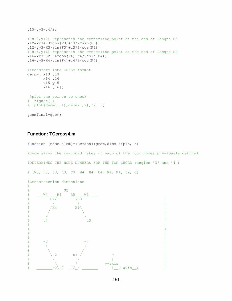
161
y15=yy3-t4/2; %(x12,y12) represents the centerline point at the e nd of length H3 x12=xx3+H3*cos(F3)+t3/2*sin(F3); y12=yy3-H3*sin(F3)+t3/2*cos(F3); %(x16,y16) represents the centerline point at the e nd of length H4 x16=xx3-S2-H4*cos(F4)-t4/2*sin(F4); y16=yy3-H4*sin(F4)+t4/2*cos(F4); %transform into CUFSM format geom=[ x13 y13 x14 y14 x15 y15 x16 y16]; %plot the points to check % figure(1) % plot(geom(:,1),geom(:,2),'k.'); geomfinal=geom;
Function: TCcross4.m
function [node,elem]=TCcross4(geom,dims,kipin, n) %geom gives the xy-coordinates of each of the four nodes previously defined %DETERMINES THE NODE NUMBERS FOR THE TOP CHORD (angles "3" and "4") % [W3, H3, t3, R3, F3, W4, H4, t4, R4, F4, S2, d] %Cross-section dimensions % % S2 % ___W4____R4 R5____W3____ % F4/ \F3 | % / \ | % /H4 H3\ | % / \ | % / \ | % t4 t3 | % | % d % | % | % t2 t1 | % \ / | % \ / | % \H2 H1 / ^ | % \ / | | % \ / y-axis | % _______F2\R2 R1/_F1_______ |__x-axis__> |
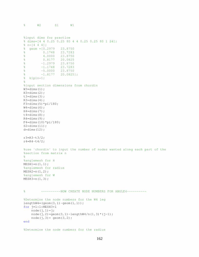
162
% W2 S1 W1 %input dims for practice % dims=[4 4 0.25 0.25 80 4 4 0.25 0.25 80 1 24]; % n=[4 4 4]; % geom =[0.2979 23.8750 % 0.1748 23.7283 % 4.0000 23.8750 % 0.8177 20.0825 % -1.2979 23.8750 % -1.1748 23.7283 % -5.0000 23.8750 % -1.8177 20.0825]; % kipin=1; % %input section dimensions from chordin W3=dims(1); H3=dims(2); t3=dims(3); R3=dims(4); F3=dims(5)*pi/180; W4=dims(6); H4=dims(7); t4=dims(8); R4=dims(9); F4=dims(10)*pi/180; S2=dims(11); d=dims(12); r3=R3-t3/2; r4=R4-t4/2; %use 'chordin' to input the number of nodes wanted along each part of the %section from matrix n % %anglemesh for H MESH1=n(1,1); %anglemesh for radius MESH2=n(1,2); %anglemesh for W MESH3=n(1,3); % ----------NOW CREATE NODE NUMBERS FOR ANGL E4---------- %Determine the node numbers for the W4 leg lengthW4=(geom(3,1)-geom(1,1)); for j=1:1:MESH3+1 node(j,1)=j; node(j,2)=geom(3,1)-lengthW4/n(1,3)*(j-1); node(j,3)= geom(3,2); end %Determine the node numbers for the radius
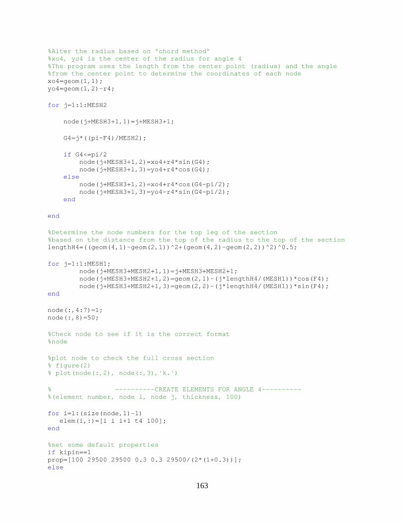
163
%Alter the radius based on "chord method" %xo4, yo4 is the center of the radius for angle 4 %The program uses the length from the center point (radius) and the angle %from the center point to determine the coordinates of each node xo4=geom(1,1); yo4=geom(1,2)-r4; for j=1:1:MESH2 node(j+MESH3+1,1)=j+MESH3+1; G4=j*((pi-F4)/MESH2); if G4<=pi/2 node(j+MESH3+1,2)=xo4+r4*sin(G4); node(j+MESH3+1,3)=yo4+r4*cos(G4); else node(j+MESH3+1,2)=xo4+r4*cos(G4-pi/2); node(j+MESH3+1,3)=yo4-r4*sin(G4-pi/2); end end %Determine the node numbers for the top leg of the section %based on the distance from the top of the radius t o the top of the section lengthH4=((geom(4,1)-geom(2,1))^2+(geom(4,2)-geom(2 ,2))^2)^0.5; for j=1:1:MESH1; node(j+MESH3+MESH2+1,1)=j+MESH3+MESH2+1; node(j+MESH3+MESH2+1,2)=geom(2,1)-(j*length H4/(MESH1))*cos(F4); node(j+MESH3+MESH2+1,3)=geom(2,2)-(j*length H4/(MESH1))*sin(F4); end node(:,4:7)=1; node(:,8)=50; %Check node to see if it is the correct format %node %plot node to check the full cross section % figure(2) % plot(node(:,2), node(:,3),'k.') % ----------CREATE ELEMENTS FOR ANGL E 4---------- %(element number, node i, node j, thickness, 100) for i=1:(size(node,1)-1) elem(i,:)=[i i i+1 t4 100]; end %set some default properties if kipin==1 prop=[100 29500 29500 0.3 0.3 29500/(2*(1+0.3))]; else

164
prop=[100 203000 203000 0.3 0.3 203000/(2*(1+0.3))] ; end % check node % node % check elem % elem
Function: TCassem4.m
function [FEn,FEe,nodeBC,TCload,BP,TCbat,CHORDcon,CHORDcount ,cLoad,RR]=TCassem4(nodestack,elemstack,tstack,FEn,FEe,s,depth,change,SEAT,no deBC,N,n,TCload,Ltc,BracePts,TCbatpos,numbattens,BP,TCbat,webcon,W,CHORDcon,C HORDcount,ii,cLoad,pinend,FCL,clip_space,RR) %Assemble the TC nodes and elements into the GLOBAL FEnode and FEelement %Change matrix values into their single values for easy use in this program depth=depth(ii,1); SEAT=SEAT(ii,1); %Chord members %-----NODES FOR THE CHORD MEMBERS----- chord1=nodestack{1}; counter=size(FEn,1); begloop=size(FEn,1)+1; %Determine where the first node in the TC is counter2=20000000+100000000*(ii-1); %Before node %Determine the number of nodes to be looped within the SEAT to %establish a boundary condition less=1.0; %the distance subtracted from SEAT to terminate the loop that determines the amount of nodes at the boundary cond ition support=SEAT+less; %The length of chord involved at the support for i=1:size(chord1,1) FEn(i+counter,1)=chord1(i,1)+counter2; %within node FEn(i+counter,2)=chord1(i,2); %x coordinate FEn(i+counter,3)=chord1(i,3)-depth; %y coordinate FEn(i+counter,4)=chord1(i,4)+s; %z coordinate plus the gap in between the chord %Write a loop to determine at which node the seat e nds in the TC (at %the beginning of the TC) x=FEn(i+counter,2); begseat=FEn(1+counter,1); if x<support endseat=FEn(i+counter,1); endloop=size(FEn,1); end end

165
%-----elements for this chord----- ecount=size(FEe,1); enum=FEe(ecount,1); for i=1:size(elemstack{1},1) FEe(i+ecount,1)=(i+enum); FEe(i+ecount,2:10)=elemstack{1}(i,2:10)+counter2 ; %within element FEe(i+ecount,11)=elemstack{1}(i,11); FEe(i+ecount,12)=elemstack{1}(i,12); FEe(i+ecount,13)=tstack{1}(1,1); end %-----BOUDARY CONDITIONS----- %Nodes in boundary condition at the beginning of th e TC %Create a nodeset for those nodes that will be at t he ends of the joist %The nodes along the bottom of the chord within the "SEAT" region are %assumed to be pinned %Determine the nodes that are at the boundary condi tions anode=3; %The number of nodes in each "pinned" element nodes=N+1; %The following loop loops around the number of node s in each cross %section and pulls out the nodes that correspond to the last element in %each cross section (for the length of the seat) for i=begloop:1:endloop nodeset(i-(begloop-1),1)=FEn(i,1); rowcount=size(nodeset,1); num=nodeset(i-counter,1)-counter2; n1=nodes; r1=rem(rowcount,n1); %Remainder function to determine what node we are at in the cross-section if r1==0 %If the remainder is zero we are at the last node i n this set newset(i-(begloop-1)-4:i-(begloop-1),1) =FEn(i-4:i,1); %The amount of nodes within the cross section that will be pinn ed end end [~,~,newset]=find(newset); %Eliminates the zeros from this array xbc=size(nodeBC); next=xbc(1,2); nodeBC{next+1}=newset(:,1); %****NODES IN THE TC AT THE END OF THE JOIST pinend=pinend-less; %Move the same distance away from the web member as on the opposing side endjoist=size(FEn,1); ENDBC=find(FEn(begloop:1:endjoist,2)>=pinend); %Determines the number of nodes that are greater than the largest x-value of of the web-members %Determine the amount of nodes that need to be loop ed around for the %end-boundary-condition subtract=size(ENDBC,1); floop=endjoist-subtract;

166
%Loop around those last nodes to apply the boundary condition for i=floop:1:endjoist nodeset(i-(begloop-1),1)=FEn(i,1); rowcount=size(nodeset,1); num=nodeset(i-counter,1)-counter2; n1=nodes; r1=rem(rowcount,n1); if r1==0 newset2(i-(begloop-1)-2:i-(begloop- 1),1)=FEn(i-2:i,1); end end [~,~,newset2]=find(newset2); %Eliminates the zeros from this array xbc=size(nodeBC); next=xbc(1,2); nodeBC{next+1}=newset2(:,1); %------ROTATIONAL RESTRAINT------- %This section applies a rotational restraint at the beginning/end of the %joist %***BEGINNING OF THE JOIST*** rx=4; %the distance in the x-diretion that the rotational restraint applies to ENDr=find(FEn(begloop:1:endjoist,2)<=rx)-nodes+ 1+counter; %find the first node in each cross-section that has a coordinate cl osest to the rotational restraint length last=max(ENDr); ext=n(1,1); %Loop around the node values less than the rotation al restraint %distance to collect all of these values for i=begloop:nodes:last ali=size(RR); next=ali(1,2); RR{next+1}=FEn(i:i+ext,1); end %***END OF THE JOIST*** maxx=max(FEn(begloop:1:endjoist,2)); %The maximum x-coordinate in the TC BEGr=find(FEn(begloop:1:endjoist,2)>=maxx-rx)+c ounter; %find the first node in each cross-section that has a coordinate cl osest to the rotational restraint length for i=BEGr:nodes:endjoist ali=size(RR); next=ali(1,2); RR{next+1}=FEn(i:i+ext,1); end %---------TC LOADING--------

167
%*****UNIFORM PRESSURE LOAD***** %For a pressure load -- get this working and get it working with the same %chord being loaded on each joist before changing i t to a symmetric loading %-----TOP CHORD LOADING----- %Determine the appropriate elements to load the top chord of the joist csize=size(FEe,1)-ecount; endloop=csize*n(1,1)/N; for i=1:endloop chordload(i,1)=FEe(i+ecount); end xbc=size(TCload); next=xbc(1,2); TCload{next+1}=chordload; %*****CONCENTRATED LOADS AT CLIPS***** %Use this load for a symmetric loading (both clips on the outside) which %simulates the VTJC tests from summer 2011 % %For other loading cases (such as if simulating fie ld conditions) where %clips are on the same side of the chord for each j oist, this part should %be neglected and TCassem3 should be used to apply all loads % %This also is useful for finding the nodes used at clip locations so that %springs can be inserted here %If you want the clips on the outside then use this code numclip=round((Ltc)/clip_space); %The number of clips per chord (one every 24"(roughly)) initial=FCL; %use the measured value from test results loadnode=n(1,1)/2; %the node in the cross section that the load is to be applied to sub=N-loadnode; %Determine the x-location of the clips along the le ngth of the chord for i=1:numclip xclip(i,1)=initial+clip_space*(i-1) ; %The clip placement occurs about every 2' end %***PT LOADS APPLIED TO THE INSIDE CHORD OF THE JOI ST*** % if ii==2 %This is specific to VTJC summer 2011 te sts, it should not be used to simulate other situations % loadcount=size(cLoad,1); % for k=1:numclip % for j=counter:1:size(FEn,1) % xx=xclip(k,1); % if FEn(j,2)<xx % %Determine the size of cLoad that has already been created % TCcload=size(FEn(1:j,1),1); % xnode=TCcload-sub;
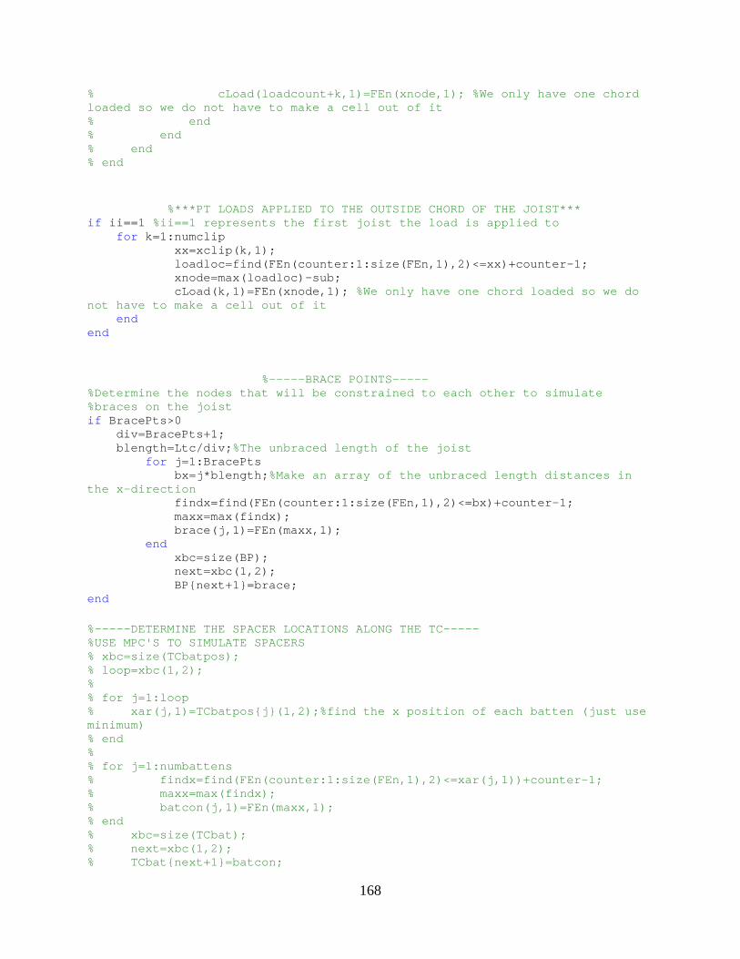
168
% cLoad(loadcount+k,1)=FEn(xnode,1) ; %We only have one chord loaded so we do not have to make a cell out of it % end % end % end % end %***PT LOADS APPLIED TO THE OUTSIDE CHORD OF THE JO IST*** if ii==1 %ii==1 represents the first joist the load is appli ed to for k=1:numclip xx=xclip(k,1); loadloc=find(FEn(counter:1:size(FEn,1), 2)<=xx)+counter-1; xnode=max(loadloc)-sub; cLoad(k,1)=FEn(xnode,1); %We only have one chord loaded so we do not have to make a cell out of it end end %-----BRACE POINTS----- %Determine the nodes that will be constrained to ea ch other to simulate %braces on the joist if BracePts>0 div=BracePts+1; blength=Ltc/div; %The unbraced length of the joist for j=1:BracePts bx=j*blength; %Make an array of the unbraced length distances in the x-direction findx=find(FEn(counter:1:size(FEn,1),2) <=bx)+counter-1; maxx=max(findx); brace(j,1)=FEn(maxx,1); end xbc=size(BP); next=xbc(1,2); BP{next+1}=brace; end %-----DETERMINE THE SPACER LOCATIONS ALONG THE TC-- --- %USE MPC'S TO SIMULATE SPACERS % xbc=size(TCbatpos); % loop=xbc(1,2); % % for j=1:loop % xar(j,1)=TCbatpos{j}(1,2);%find the x positio n of each batten (just use minimum) % end % % for j=1:numbattens % findx=find(FEn(counter:1:size(FEn,1),2)<= xar(j,1))+counter-1; % maxx=max(findx); % batcon(j,1)=FEn(maxx,1); % end % xbc=size(TCbat); % next=xbc(1,2); % TCbat{next+1}=batcon;

169
xbc=size(TCbatpos); loop=xbc(1,2); for j=1:loop xar(j,1)=TCbatpos{j}(1,2); %find the x position of each spacer (just use minimum) end %Determine the number of nodes to use for each spac er (just use the entire %vertical face of each angle in the chord) splen=n(1,3); %The number of nodes along the vertical face of the angle in the TC in addition to the one that is already selected %number of elements+1=number of nodes (but we alrea dy have %one of the nodes so we just need to add the additi onal %amount to the set) %We need to grab the nodes for each spacer. To do t his let's find the node %in the chord that is closest to the x-coordinate o f the spacer and grab %every node on that vertical face of the angle tick=1; for j=1:splen+1:numbattens*(splen+1) findx=find(FEn(counter:1:size(FEn,1),2)<=xa r(tick,1))+counter-1; %find the nodes in FEn that are closest to each spacer (x -coordinate) maxx=max(findx); %Find the closest node batcon(j:j+splen,1)=FEn(maxx-splen:maxx,1); %Get all of the nodes for each spacer (maxx-splen:maxx is to grab every node along a single face of each angle) tick=tick+1; end xbc=size(TCbat); next=xbc(1,2); TCbat{next+1}=batcon; %-----CONSTRAIN THE CHORDS TO THE WEB MEMBERS----- %Determine where to constrain the web members with these node sets! kqn=size(webcon); loo=kqn(1,2)/ii; %the loop size for determining the node sets for i=1:loo for j=1:size(webcon{i},1) if webcon{i}(j,3)>-depth/2; xweb=webcon{i}(j,2); %The x value that the chord must be less than to be constrained to %Now loop around the nodes in TC3 until you find a winner! for k=counter:1:size(FEn,1); if FEn(k,2)<xweb if webcon{i}(j,4)<W/2 CHORDcon(i,:)=FEn(k,:); CHORDcount(i,1)=k; end end end
170
end end end end
Function: BCxy1.m
function [geomfinal]=BCxy1(dims) %LTC %March 2011 %Takes out to out dimensions and corner angles of c omponents of the cross %section of a joist and converts them to xy coordin ates for use in CUFSM %To measure F you can find the angle of each segmen t from vertical (H & W) %then determine the difference between the two. Th e difference = F % [W1, H1, t1, R1, F1, W2, H2, t2, R2, F2, S1, W3, H3, t3, R3, F3, W4, H4, t4, R4, F4, S2, d] %input dims for practice % dims=[4 4 .25 .25 80 4 4 0.25 0.25 80 1]; %Cross-section dimensions % % t2 t1 % \ / % \ / % \H2 H1 / ^ % \ / | % \ / y-axis % _______F2\R2 R1/_F1_______ |__Z-axis__> % W2 S1 W1 % [W1, H1, t1, R1, F1, W2, H2, t2, R2, F2, S1, W3, H3, t3, R3, F3, W4, H4, % t4, R4, F4, S2, d] W1=dims(1); H1=dims(2); t1=dims(3); R1=dims(4); F1=dims(5)*pi/180; W2=dims(6); H2=dims(7); t2=dims(8); R2=dims(9); F2=dims(10)*pi/180; S1=dims(11); %orgin is intersection of H1-line and W1-line %r=the centerline radius of the angle r1=R1-t1/2;
171
r2=R2-t2/2; %(x1,y1) represents the beginning of the radius on the W1-leg x1=R1/tan(F1/2); y1=t1/2; %(x5,y5) represent the beginning of the radius of t he W2-leg x5=-S1-R2/tan(F2/2); y5=t2/2; %(xc, yc) represents the center of the arc 1 xc=x1; yc=y1+r1; %(xc2, yc2) represents the center of the arc 2 xc2=x5; yc2=y5+r2; %(x2,y2) represents the beginning of the radius on the H1-leg G=pi-F1; if G<=pi/2 x2=xc-r1*sin(G); y2=yc-r1*cos(G); else x2=xc-r1*cos(G-pi/2); y2=yc+r1*sin(G-pi/2); end %(x6,y6) represents the beginning of the radius on the H2-leg G2=pi-F2; if G2<=pi/2 x6=xc2+r2*sin(G2); y6=yc2-r2*cos(G2); else x6=xc2+r2*cos(G2-pi/2); y6=yc2+r2*sin(G2-pi/2); end %(x3,y3) represents the centerline point at the end of length W1 x3=W1; y3=t1/2; %(x7,y7) represents the centerline point at the end of length W2 x7=-W2-S1; y7=t2/2; %(x4,y4) represents the centerline point at the end of length H1 x4=H1*cos(F1)+t1/2*sin(F1); y4=H1*sin(F1)-t1/2*cos(F1); %(x8,y8) represents the centerline point at the end of length H2 x8=-S1-H2*cos(F2)-t2/2*sin(F2); y8=H2*sin(F2)-t2/2*cos(F2); %transform into CUFSM format geom=[ x1 y1 x2 y2

172
x3 y3 x4 y4]; %plot the points to check % figure(1) % plot(geom(:,1),geom(:,2),'k.'); geomfinal=geom;
Function: BCcross1.m
function [node,elem]=BCcross1(geom,dims,kipin, n) %geom gives the xy-coordinates of each of the four nodes previously defined %This program determines nodes for "angle 1" first, then determines the %node numbers for "angle 2" % [W1, H1, t1, R1, F1, W2, H2, t2, R2, F2, S1] %Cross-section dimensions % % t2 t1 % \ / % \ / % \H2 H1 / ^ % \ / | % \ / y-axis % _______F2\R2 R1/_F1_______ |__z-axis__> % W2 S1 W1 %input dims for practice % dims=[4 4 .25 .25 80 4 4 0.25 0.25 80 1 4 4 0.25 0.25 80 4 4 0.25 0.25 80 1 24]; % n=[4 4 4]; % geom =[0.2979 0.1250 % 0.1748 0.2717 % 4.0000 0.1250 % 0.8177 3.9175 % -1.2979 0.1250 % -1.1748 0.2717 % -5.0000 0.1250 % -1.8177 3.9175]; % kipin=1; %input section dimensions from chordin W1=dims(1); H1=dims(2); t1=dims(3); R1=dims(4); F1=dims(5)*pi/180;
173
W2=dims(6); H2=dims(7); t2=dims(8); R2=dims(9); F2=dims(10)*pi/180; S1=dims(11); r1=R1-t1/2; r2=R2-t2/2; %use 'chordin' to input the number of nodes wanted along each part of the %section from matrix n % %anglemesh for H MESH1=n(1,1); %anglemesh for radius MESH2=n(1,2); %anglemesh for W MESH3=n(1,3); % ------------CREATE NODE NUMBERS FOR ANGLE 1------ ---------- %Determine the node numbers for the W leg lengthW=(geom(3,1)-geom(1,1)); for j=1:1:MESH3+1 node(j,1)=j; node(j,2)=geom(3,1)-lengthW/n(1,3)*(j-1); node(j,3)= geom(3,2); end %Determine the node numbers for the radius %Alter the radius based on "chord method" %xo, yo is the center of the radius %The program uses the length from the center point (radius) and the angle %from the center point to determine the coordinates of each node xo=geom(1,1); yo=geom(1,2)+r1; for j=1:1:MESH2 node(j+MESH3+1,1)=j+MESH3+1; G=j*((pi-F1)/MESH2); if G<=pi/2 node(j+MESH3+1,2)=xo-r1*sin(G); node(j+MESH3+1,3)=yo-r1*cos(G); else node(j+MESH3+1,2)=xo-r1*cos(G-pi/2); node(j+MESH3+1,3)=yo+r1*sin(G-pi/2); end end
174
%Determine the node numbers for the top leg of the section %based on the distance from the top of the radius t o the top of the section lengthH=((geom(4,1)-geom(2,1))^2+(geom(4,2)-geom(2, 2))^2)^0.5; for j=1:1:MESH1; node(j+MESH3+MESH2+1,1)=j+MESH3+MESH2+1; node(j+MESH3+MESH2+1,2)=geom(2,1)+(j*length H/(MESH1))*cos(F1); node(j+MESH3+MESH2+1,3)=geom(2,2)+(j*length H/(MESH1))*sin(F1); end node(:,4:7)=1; node(:,8)=50; %Check node to see if it is the correct format %node %plot node to check frist angle % figure(2) % plot(node(:,2), node(:,3),'k.') % ----------CREATE ELEMENTS FOR ANGL E 1---------- %(element number, node i, node j, thickness, 100) for i=1:(size(node,1)-1) elem(i,:)=[i i i+1 t1 100]; end % elem % check node % node % check elem % elem
Function: BCassem1.m
function [FEn,FEe,BP,BCbat,CHORDcon,CHORDcount,nodeBC,midx]= BCassem1(nodestack,elemstack,tstack,FEn,FEe,BC,s,depth,change,SEAT,SPACE,GAP, Ltc,BracePts,BCbatpos,numbattens,BP,webcon,W,CHORDcon,CHORDcount,ii,BCbat,N,n odeBC,pinend,midx,n) %Add the nodes and elements for the bottom chord in to the GLOBAL node and %element matrices %Change matrix values into their single values for easy use in this program depth=depth(ii); SEAT=SEAT(ii); BC=BC(ii);
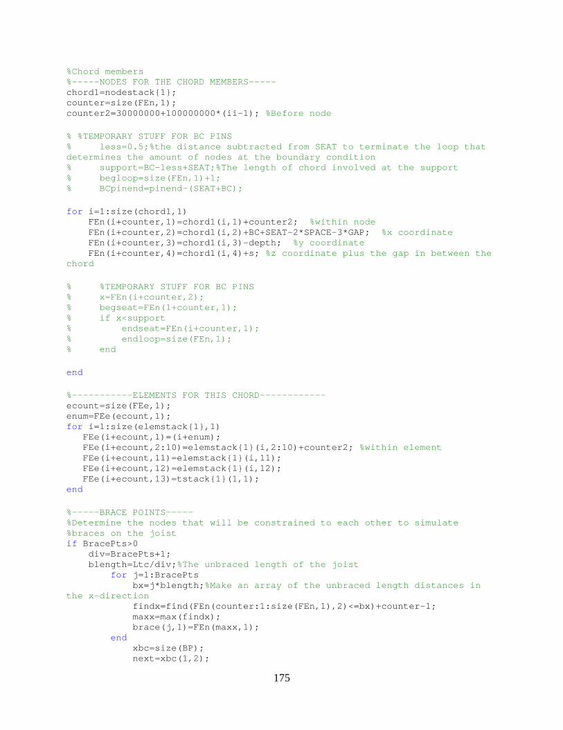
175
%Chord members %-----NODES FOR THE CHORD MEMBERS----- chord1=nodestack{1}; counter=size(FEn,1); counter2=30000000+100000000*(ii-1); %Before node % %TEMPORARY STUFF FOR BC PINS % less=0.5;%the distance subtracted from SEAT t o terminate the loop that determines the amount of nodes at the boundary cond ition % support=BC-less+SEAT;%The length of chord inv olved at the support % begloop=size(FEn,1)+1; % BCpinend=pinend-(SEAT+BC); for i=1:size(chord1,1) FEn(i+counter,1)=chord1(i,1)+counter2; %within node FEn(i+counter,2)=chord1(i,2)+BC+SEAT-2*SPACE-3* GAP; %x coordinate FEn(i+counter,3)=chord1(i,3)-depth; %y coordinate FEn(i+counter,4)=chord1(i,4)+s; %z coordinate plus the gap in between the chord % %TEMPORARY STUFF FOR BC PINS % x=FEn(i+counter,2); % begseat=FEn(1+counter,1); % if x<support % endseat=FEn(i+counter,1); % endloop=size(FEn,1); % end end %-----------ELEMENTS FOR THIS CHORD------------ ecount=size(FEe,1); enum=FEe(ecount,1); for i=1:size(elemstack{1},1) FEe(i+ecount,1)=(i+enum); FEe(i+ecount,2:10)=elemstack{1}(i,2:10)+counter2 ; %within element FEe(i+ecount,11)=elemstack{1}(i,11); FEe(i+ecount,12)=elemstack{1}(i,12); FEe(i+ecount,13)=tstack{1}(1,1); end %-----BRACE POINTS----- %Determine the nodes that will be constrained to ea ch other to simulate %braces on the joist if BracePts>0 div=BracePts+1; blength=Ltc/div; %The unbraced length of the joist for j=1:BracePts bx=j*blength; %Make an array of the unbraced length distances in the x-direction findx=find(FEn(counter:1:size(FEn,1),2) <=bx)+counter-1; maxx=max(findx); brace(j,1)=FEn(maxx,1); end xbc=size(BP); next=xbc(1,2);

176
BP{next+1}=brace; end %-----DETERMINE THE SPACER LOCATIONS ALONG THE BC-- --- %USE MPC'S TO SIMULATE SPACERS xbc=size(BCbatpos); loop=xbc(1,2); j=loop; xar(j,1)=BCbatpos{j}(1,2); %find the x position of each spacer (just use minimum) splen=n(1,3); %The number of nodes along the vertical face of the angle in the TC in addition to the one that is already selected %number of elements+1=number of nodes (but we alrea dy have %one of the nodes so we just need to add the additi onal %amount to the set) findx=find(FEn(counter:1:size(FEn,1),2)<=xar(j,1))+ counter-1; maxx=max(findx); batcon(j:j+splen,1)=FEn(maxx-splen:maxx,1); if ii==1 BCbat{1}=batcon; else xbc=size(BCbat); next=xbc(1,2); BCbat{next+1}=batcon; end %-------------DEFLECTION MONITOR------------- %Find the node that is closest to midspan to monito r its deflection %By monitoring this node we will be able to determi ne when the joist %buckles % %We already found the node at mid-span (because of the spacer) so let's %just use this to monitor the displacement %Find the node that is closest to midspan to monito r its deflection % %We only need to monitor the deflection on one chor d only (this is the only %monitor in the bottom chord for THIS JOIST) (one i s made for each joist) midnode=FEn(maxx,1); %The node with the x-coordinate that is closest to mid-span if ii==1 midx{1}=midnode; else xbc=size(midx); next=xbc(1,2); midx{next+1}=midnode; end %-----CONSTRAIN THE CHORDS TO THE WEB MEMBERS-----
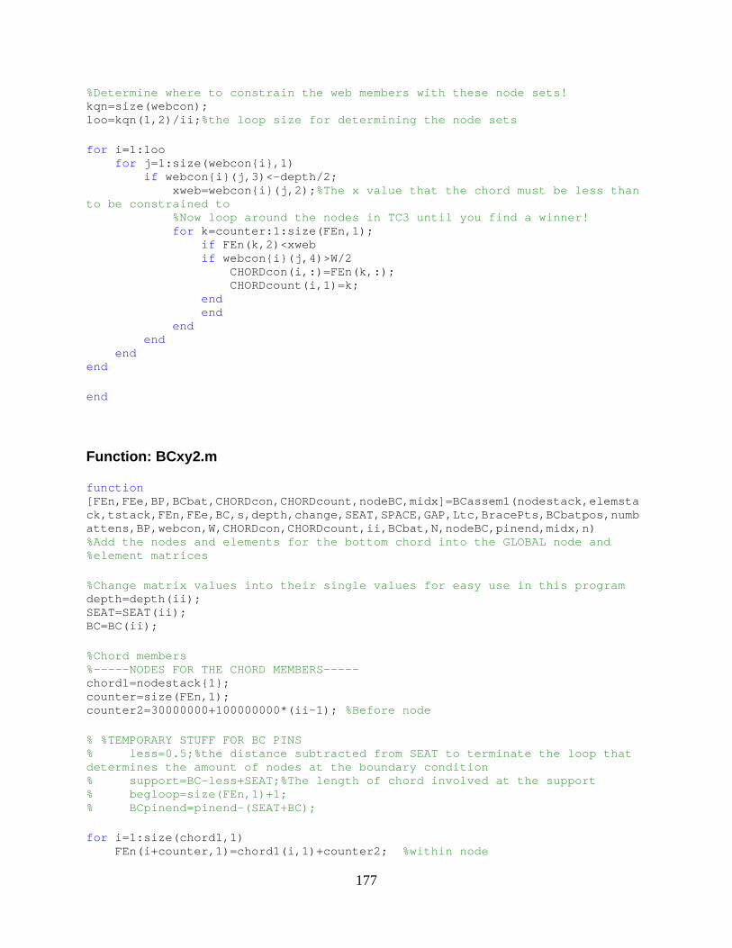
177
%Determine where to constrain the web members with these node sets! kqn=size(webcon); loo=kqn(1,2)/ii; %the loop size for determining the node sets for i=1:loo for j=1:size(webcon{i},1) if webcon{i}(j,3)<-depth/2; xweb=webcon{i}(j,2); %The x value that the chord must be less than to be constrained to %Now loop around the nodes in TC3 until you find a winner! for k=counter:1:size(FEn,1); if FEn(k,2)<xweb if webcon{i}(j,4)>W/2 CHORDcon(i,:)=FEn(k,:); CHORDcount(i,1)=k; end end end end end end end
Function: BCxy2.m
function [FEn,FEe,BP,BCbat,CHORDcon,CHORDcount,nodeBC,midx]= BCassem1(nodestack,elemstack,tstack,FEn,FEe,BC,s,depth,change,SEAT,SPACE,GAP, Ltc,BracePts,BCbatpos,numbattens,BP,webcon,W,CHORDcon,CHORDcount,ii,BCbat,N,n odeBC,pinend,midx,n) %Add the nodes and elements for the bottom chord in to the GLOBAL node and %element matrices %Change matrix values into their single values for easy use in this program depth=depth(ii); SEAT=SEAT(ii); BC=BC(ii); %Chord members %-----NODES FOR THE CHORD MEMBERS----- chord1=nodestack{1}; counter=size(FEn,1); counter2=30000000+100000000*(ii-1); %Before node % %TEMPORARY STUFF FOR BC PINS % less=0.5;%the distance subtracted from SEAT t o terminate the loop that determines the amount of nodes at the boundary cond ition % support=BC-less+SEAT;%The length of chord inv olved at the support % begloop=size(FEn,1)+1; % BCpinend=pinend-(SEAT+BC); for i=1:size(chord1,1) FEn(i+counter,1)=chord1(i,1)+counter2; %within node
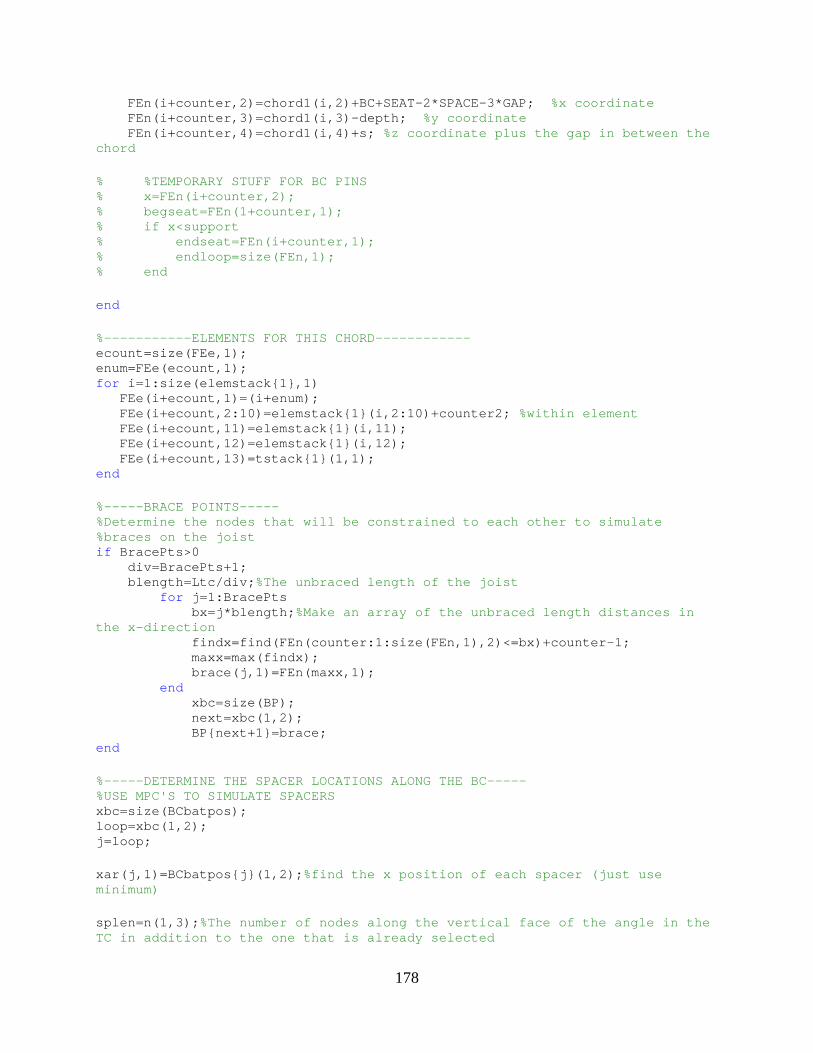
178
FEn(i+counter,2)=chord1(i,2)+BC+SEAT-2*SPACE-3* GAP; %x coordinate FEn(i+counter,3)=chord1(i,3)-depth; %y coordinate FEn(i+counter,4)=chord1(i,4)+s; %z coordinate plus the gap in between the chord % %TEMPORARY STUFF FOR BC PINS % x=FEn(i+counter,2); % begseat=FEn(1+counter,1); % if x<support % endseat=FEn(i+counter,1); % endloop=size(FEn,1); % end end %-----------ELEMENTS FOR THIS CHORD------------ ecount=size(FEe,1); enum=FEe(ecount,1); for i=1:size(elemstack{1},1) FEe(i+ecount,1)=(i+enum); FEe(i+ecount,2:10)=elemstack{1}(i,2:10)+counter2 ; %within element FEe(i+ecount,11)=elemstack{1}(i,11); FEe(i+ecount,12)=elemstack{1}(i,12); FEe(i+ecount,13)=tstack{1}(1,1); end %-----BRACE POINTS----- %Determine the nodes that will be constrained to ea ch other to simulate %braces on the joist if BracePts>0 div=BracePts+1; blength=Ltc/div; %The unbraced length of the joist for j=1:BracePts bx=j*blength; %Make an array of the unbraced length distances in the x-direction findx=find(FEn(counter:1:size(FEn,1),2) <=bx)+counter-1; maxx=max(findx); brace(j,1)=FEn(maxx,1); end xbc=size(BP); next=xbc(1,2); BP{next+1}=brace; end %-----DETERMINE THE SPACER LOCATIONS ALONG THE BC-- --- %USE MPC'S TO SIMULATE SPACERS xbc=size(BCbatpos); loop=xbc(1,2); j=loop; xar(j,1)=BCbatpos{j}(1,2); %find the x position of each spacer (just use minimum) splen=n(1,3); %The number of nodes along the vertical face of the angle in the TC in addition to the one that is already selected
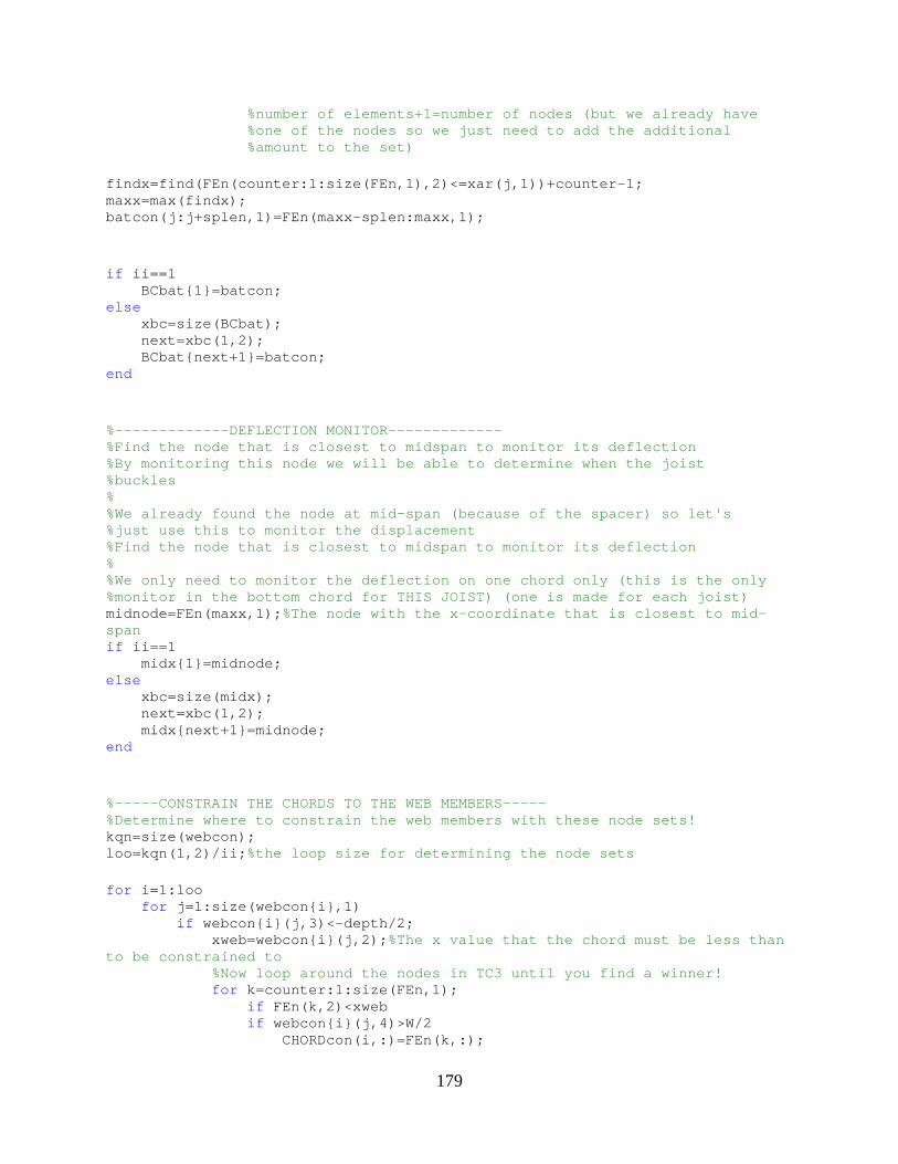
179
%number of elements+1=number of nodes (but we alrea dy have %one of the nodes so we just need to add the additi onal %amount to the set) findx=find(FEn(counter:1:size(FEn,1),2)<=xar(j,1))+ counter-1; maxx=max(findx); batcon(j:j+splen,1)=FEn(maxx-splen:maxx,1); if ii==1 BCbat{1}=batcon; else xbc=size(BCbat); next=xbc(1,2); BCbat{next+1}=batcon; end %-------------DEFLECTION MONITOR------------- %Find the node that is closest to midspan to monito r its deflection %By monitoring this node we will be able to determi ne when the joist %buckles % %We already found the node at mid-span (because of the spacer) so let's %just use this to monitor the displacement %Find the node that is closest to midspan to monito r its deflection % %We only need to monitor the deflection on one chor d only (this is the only %monitor in the bottom chord for THIS JOIST) (one i s made for each joist) midnode=FEn(maxx,1); %The node with the x-coordinate that is closest to mid-span if ii==1 midx{1}=midnode; else xbc=size(midx); next=xbc(1,2); midx{next+1}=midnode; end %-----CONSTRAIN THE CHORDS TO THE WEB MEMBERS----- %Determine where to constrain the web members with these node sets! kqn=size(webcon); loo=kqn(1,2)/ii; %the loop size for determining the node sets for i=1:loo for j=1:size(webcon{i},1) if webcon{i}(j,3)<-depth/2; xweb=webcon{i}(j,2); %The x value that the chord must be less than to be constrained to %Now loop around the nodes in TC3 until you find a winner! for k=counter:1:size(FEn,1); if FEn(k,2)<xweb if webcon{i}(j,4)>W/2 CHORDcon(i,:)=FEn(k,:);
180
CHORDcount(i,1)=k; end end end end end end end
Function: BCcross2.m
function [FEn,FEe,BP,BCbat,CHORDcon,CHORDcount,nodeBC,midx]= BCassem1(nodestack,elemstack,tstack,FEn,FEe,BC,s,depth,change,SEAT,SPACE,GAP, Ltc,BracePts,BCbatpos,numbattens,BP,webcon,W,CHORDcon,CHORDcount,ii,BCbat,N,n odeBC,pinend,midx,n) %Add the nodes and elements for the bottom chord in to the GLOBAL node and %element matrices %Change matrix values into their single values for easy use in this program depth=depth(ii); SEAT=SEAT(ii); BC=BC(ii); %Chord members %-----NODES FOR THE CHORD MEMBERS----- chord1=nodestack{1}; counter=size(FEn,1); counter2=30000000+100000000*(ii-1); %Before node % %TEMPORARY STUFF FOR BC PINS % less=0.5;%the distance subtracted from SEAT t o terminate the loop that determines the amount of nodes at the boundary cond ition % support=BC-less+SEAT;%The length of chord inv olved at the support % begloop=size(FEn,1)+1; % BCpinend=pinend-(SEAT+BC); for i=1:size(chord1,1) FEn(i+counter,1)=chord1(i,1)+counter2; %within node FEn(i+counter,2)=chord1(i,2)+BC+SEAT-2*SPACE-3* GAP; %x coordinate FEn(i+counter,3)=chord1(i,3)-depth; %y coordinate FEn(i+counter,4)=chord1(i,4)+s; %z coordinate plus the gap in between the chord % %TEMPORARY STUFF FOR BC PINS % x=FEn(i+counter,2); % begseat=FEn(1+counter,1); % if x<support % endseat=FEn(i+counter,1); % endloop=size(FEn,1); % end end

181
%-----------ELEMENTS FOR THIS CHORD------------ ecount=size(FEe,1); enum=FEe(ecount,1); for i=1:size(elemstack{1},1) FEe(i+ecount,1)=(i+enum); FEe(i+ecount,2:10)=elemstack{1}(i,2:10)+counter2 ; %within element FEe(i+ecount,11)=elemstack{1}(i,11); FEe(i+ecount,12)=elemstack{1}(i,12); FEe(i+ecount,13)=tstack{1}(1,1); end %-----BRACE POINTS----- %Determine the nodes that will be constrained to ea ch other to simulate %braces on the joist if BracePts>0 div=BracePts+1; blength=Ltc/div; %The unbraced length of the joist for j=1:BracePts bx=j*blength; %Make an array of the unbraced length distances in the x-direction findx=find(FEn(counter:1:size(FEn,1),2) <=bx)+counter-1; maxx=max(findx); brace(j,1)=FEn(maxx,1); end xbc=size(BP); next=xbc(1,2); BP{next+1}=brace; end %-----DETERMINE THE SPACER LOCATIONS ALONG THE BC-- --- %USE MPC'S TO SIMULATE SPACERS xbc=size(BCbatpos); loop=xbc(1,2); j=loop; xar(j,1)=BCbatpos{j}(1,2); %find the x position of each spacer (just use minimum) splen=n(1,3); %The number of nodes along the vertical face of the angle in the TC in addition to the one that is already selected %number of elements+1=number of nodes (but we alrea dy have %one of the nodes so we just need to add the additi onal %amount to the set) findx=find(FEn(counter:1:size(FEn,1),2)<=xar(j,1))+ counter-1; maxx=max(findx); batcon(j:j+splen,1)=FEn(maxx-splen:maxx,1); if ii==1 BCbat{1}=batcon; else xbc=size(BCbat); next=xbc(1,2);
182
BCbat{next+1}=batcon; end %-------------DEFLECTION MONITOR------------- %Find the node that is closest to midspan to monito r its deflection %By monitoring this node we will be able to determi ne when the joist %buckles % %We already found the node at mid-span (because of the spacer) so let's %just use this to monitor the displacement %Find the node that is closest to midspan to monito r its deflection % %We only need to monitor the deflection on one chor d only (this is the only %monitor in the bottom chord for THIS JOIST) (one i s made for each joist) midnode=FEn(maxx,1); %The node with the x-coordinate that is closest to mid-span if ii==1 midx{1}=midnode; else xbc=size(midx); next=xbc(1,2); midx{next+1}=midnode; end %-----CONSTRAIN THE CHORDS TO THE WEB MEMBERS----- %Determine where to constrain the web members with these node sets! kqn=size(webcon); loo=kqn(1,2)/ii; %the loop size for determining the node sets for i=1:loo for j=1:size(webcon{i},1) if webcon{i}(j,3)<-depth/2; xweb=webcon{i}(j,2); %The x value that the chord must be less than to be constrained to %Now loop around the nodes in TC3 until you find a winner! for k=counter:1:size(FEn,1); if FEn(k,2)<xweb if webcon{i}(j,4)>W/2 CHORDcon(i,:)=FEn(k,:); CHORDcount(i,1)=k; end end end end end end end

183
Function: BCassem2.m
function [FEn,FEe,BP,BCbat,CHORDcon,CHORDcount,nodeBC]=BCass em2(nodestack,elemstack,tstack,FEn,FEe,BC,s,depth,change,SEAT,SPACE,GAP,Ltc,B racePts,BCbatpos,numbattens,BP,BCbat,webcon,W,CHORDcon,CHORDcount,ii,N,nodeBC ,pinend,n) %Add the nodes and elements for the bottom chord in to the GLOBAL node and %element matrices %Change matrix values into their single values for easy use in this program depth=depth(ii,1); SEAT=SEAT(ii,1); BC=BC(ii); %Chord members %-----NODES FOR THE CHORD MEMBERS----- chord1=nodestack{1}; counter=size(FEn,1); counter2=40000000+100000000*(ii-1); %Before node % % %TEMPORARY STUFF FOR BC PINS % less=0.5;%the distance subtracted from SEAT t o terminate the loop that determines the amount of nodes at the boundary cond ition % support=BC-less+SEAT;%The length of chord inv olved at the support % begloop=size(FEn,1)+1; % BCpinend=pinend-(SEAT+BC); for i=1:size(chord1,1) FEn(i+counter,1)=chord1(i,1)+counter2; %within node FEn(i+counter,2)=chord1(i,2)+BC+SEAT-2*SPACE-3* GAP; %x coordinate FEn(i+counter,3)=chord1(i,3)-depth; %y coordinate FEn(i+counter,4)=chord1(i,4)+s; %z coordinate plus the gap in between the chord % %TEMPORARY STUFF FOR BC PINS % x=FEn(i+counter,2); % begseat=FEn(1+counter,1); % if x<support % endseat=FEn(i+counter,1); % endloop=size(FEn,1); % end end %-----elements for this chord----- ecount=size(FEe,1); enum=FEe(ecount,1); for i=1:size(elemstack{1},1) FEe(i+ecount,1)=(i+enum); FEe(i+ecount,2:10)=elemstack{1}(i,2:10)+counter2 ; %within element FEe(i+ecount,11)=elemstack{1}(i,11); FEe(i+ecount,12)=elemstack{1}(i,12); FEe(i+ecount,13)=tstack{1}(1,1); end
184
%-----BRACE POINTS----- %Determine the nodes that will be constrained to ea ch other to simulate %braces on the joist if BracePts>0 div=BracePts+1; blength=Ltc/div; %The unbraced length of the joist for j=1:BracePts bx=j*blength; %Make an array of the unbraced length distances in the x-direction findx=find(FEn(counter:1:size(FEn,1),2) <=bx)+counter-1; maxx=max(findx); brace(j,1)=FEn(maxx,1); end xbc=size(BP); next=xbc(1,2); BP{next+1}=brace; end %-----DETERMINE THE SPACER LOCATIONS ALONG THE BC-- --- %USE MPC'S TO SIMULATE SPACERS xbc=size(BCbatpos); loop=xbc(1,2); j=loop; xar(j,1)=BCbatpos{j}(1,2); %find the x position of each batten (just use minimum) splen=n(1,3); %The number of nodes along the vertical face of the angle in the TC in addition to the one that is already selected %number of elements+1=number of nodes (but we alrea dy have %one of the nodes so we just need to add the additi onal %amount to the set) findx=find(FEn(counter:1:size(FEn,1),2)<=xar(j,1))+ counter-1; maxx=max(findx); batcon(j:j+splen,1)=FEn(maxx-splen:maxx,1); xbc=size(BCbat); next=xbc(1,2); BCbat{next+1}=batcon; %-----CONSTRAIN THE CHORDS TO THE WEB MEMBERS----- %Determine where to constrain the web members with these node sets! kqn=size(webcon); loo=kqn(1,2)/ii; %the loop size for determining the node sets for i=1:loo for j=1:size(webcon{i},1) if webcon{i}(j,3)<-depth/2; xweb=webcon{i}(j,2); %The x value that the chord must be less than to be constrained to %Now loop around the nodes in TC3 until you find a winner! for k=counter:1:size(FEn,1); if FEn(k,2)<xweb
185
if webcon{i}(j,4)<W/2 CHORDcon(i,:)=FEn(k,:); CHORDcount(i,1)=k; end end end end end end end
Function: jhabnl.m
function [FEnode, FEelem]= jhabnl(step, jobname,matprops, i mperfections, sectionpoints, FEnode, FEelem, eltype, webcon,nodeBC,TCload,BP,TCbat,BCbat,cLoad,LOAD_TYPE ,CHORDcon,CHORDc,n_chord,numnodes,analysis,kclip,RR,midx,EF,kroof) %This function generates eigenbuckling .inp files u sing ABAQUS S9R5 elements and the Lanczos eigensolver. %Used by VTJC for joist input into ABAQUS %CDM (with lots of help from BWS) %December 2007 %Modified by LTC for VTJC use %July 2011 %HEADING PARAMETERS title= 'Joist:24K4' ; modelname= '*Test designation' ; preprint.echo= 'NO' ; preprint.model= 'NO' ; preprint.history= 'NO' ; preprint.contact= 'NO' ; %CREATE INP FILE %open file fid=fopen([jobname '.inp' ], 'w' ); %write heading info heading(fid,title,jobname,modelname,preprint); disp( 'Header Input Complete...input file' ); matnum=100 t=0.01 elemgroups=1 %write nodes and element info to file writenodes_elements(fid, FEnode,FEelem,elemgroups,eltype,matnum,t,sectionpoi nts); disp( 'Nodes Complete....input file' );

186
maxel=max(FEelem(:,1)); %write spring element information to file writesprings(fid,cLoad,maxel,kclip,EF,kroof); %write nodeset info to file %writenodeset(fid,nodesetinfo,nodeset); %write material info to file writematerials(fid,matprops); disp( 'Write Materials Complete...input file' ); %write imperfections to file if imperfections.type~=3 writeimper(fid,imperfections); end %write surface definitions %writesurface(fid,surface,surface.areadist,nodeset) ; if LOAD_TYPE=='P' write_load_surface(fid,TCload); end %write constraints info to file writeconstraint(fid,webcon,BP,TCbat,BCbat,CHORDcon, CHORDc,FEnode,n_chord,numnodes,RR); %write boundary conditions into file writeBC(fid,nodeBC,BP); disp( 'Boundary Conditions Complete...input file' ) %write ABAQUS monitoring information to a file (thi ngs to monitor while %ABAQUS performs the analysis) writemonitor(fid,midx); %write analysis step info to file writestep(fid,step,nodeBC,LOAD_TYPE,cLoad,TCload,an alysis,midx); disp( 'Step Complete...input file' ) %close file fclose(fid);
Function: writenodes_elements.m
function writenodes_elements(fid, FEnode,FEelem,elemgroups,eltype,matnum,t,sectionpoi nts,ftcn,ltcn,ftce,ltce) %This needs to only apply to the nodes correspondin g to the tdiff values in %FEelem %save FEelem FEelem %stop %Resize elements to only include those in the TC
187
% FEelem=FEelem(ftce:ltce,:); %write nodes to file fprintf(fid, '*Node\n' ); for i=1:size(FEnode,1) fprintf(fid, '%6.0f, %6.4f, %6.4f, %6.4f\n' ,FEnode(i,1:4)); end %FEelem %stop %Make an array of the individual stiffnesses of dif ferent components within %the joist tdiff=unique(FEelem(:,13)); %check %Find the elements that correspond to these differe nt thicknesses for i=1:size(tdiff,1) copy=find(FEelem(:,13)==tdiff(i,1)); stack{i}=FEelem(copy(:,1),:); %Old, slow way that loops around all of the element s % next=0;%zeros this counter for the next i % %Use FIND to organize the materials of differ ent thicknesses into % %seperate matrices % for j=1:size(FEelem,1)%begin a loop around FE elem to find all of the elements with different thicknesses and keep them i n the array "hold" % if FEelem(j,13)==tdiff(i,1) % next=next+1; % stack{i}(next,:)=FEelem(j,:);%put the array containing the elements of like thickness into the cell stack, thi s sorts the different thickness elements which are accessed later and wri tten to the inp file % end % end end %The old way that doesn't work % for i=1:length(tdiff) % a=find(FEelem(:,13)==tdiff(i)); % begFE=a(1,1); % finFE=max(a); % stack{i}=FEelem(begFE:finFE,:); % end if eltype== 'S9R5' %write elements to file for i=1:length(tdiff) % stripel=find(FEelem(:,13)==tdiff(i)); fprintf(fid, '*Element, type=%s, ELSET=GROUP%d\n' ,char(eltype),i); fprintf(fid, '%6.0f, %6.0f, %6.0f, %6.0f, %6.0f, %6.0f, %6.0f, % 6.0f, %6.0f, %6.0f\n' ,stack{i}(:,1:10)'); fprintf(fid, '*SHELL SECTION, ELSET=GROUP%d, MATERIAL=MAT%d\n' ,[i matnum]); fprintf(fid, '%g,%g \n' ,tdiff(i),sectionpoints);
188
end elseif eltype== 'S8R5' for i=1:length(elemgroups) stripel=find(FEelem(:,11)==elemgroups(i)); fprintf(fid, '*Element, type=%s, ELSET=GROUP%d\n',char(eltype),elemgroups(i)); fprintf(fid, '%6.0f, %6.0f, %6.0f, %6.0f, %6.0f, %6.0f, %6.0f, % 6.0f, %6.0f\n' ,FEelem(stripel,1:9)'); fprintf(fid, '*SHELL SECTION, ELSET=GROUP%d, MATERIAL=MAT%d\n',[elemgroups(i) matnum(i)]); fprintf(fid, '%g,%g \n' ,t(i),sectionpoints); end end
Function: writesprings.m
%PROGRAM writesprings %This program writes spring elements to the ABAQUS input file. function writesprings(fid,cLoad,maxel,kclip,EF,kroof) % %----------------CREATE SPRINGS---TYPE I--------- ------- % loop=size(cLoad,1); % for i=1:loop % fprintf(fid,'*ELEMENT, TYPE=SPRING1, ELSE T=SPRING%d\n',i); % fprintf(fid,'%6.0f,%6.0f\n',maxel+i,cLoad (i,1)); % end % % %Give spring properties % for i=1:loop % fprintf(fid,'*SPRING, ELSET=SPRING%d\n',i ); % fprintf(fid,'3\n');%we want the spring to influence DOF 3 (displacement in the z-direction) % fprintf(fid,'%6.16f\n',kclip); % end %For SPRING1 and SPRING2 elements: %first line: DOF that the spring is resisting (3 is z-direction) %second line: spring stiffness %----------------CREATE SPRINGS---TYPE II---------- ------ %We need to connect the first joist to the second j oist numclips=size(cLoad,1)/2; %number of clips on each joist fprintf(fid, '*ELEMENT, TYPE=SPRING2, ELSET=SPRING%d\n' ,1); for i=1:numclips check=[cLoad(i,1),cLoad(i+numclips,1)]; fprintf(fid, '%6.0f,%6.0f,%6.0f\n' ,maxel+i,cLoad(i,1),cLoad(i+numclips,1)); %
189
end %Give spring properties % for i=1:numclips fprintf(fid, '*SPRING, ELSET=SPRING%d\n' ,1); fprintf(fid, '3,3\n' ); %we want the spring to influence DOF 3 (displacement in the z-direction) fprintf(fid, '%6.16f\n' ,kclip); % end % %-----------------ELASTIC FOUNDATION STIFFNESS--- ---------- % %for these apply the elastic foundation stiffness to the elements % %create different surfaces using different el ement sets for each joist % cols=size(EF); % loop=cols(1,2);%Number of cells in EF % % for i=1:loop % fprintf(fid,'*ELSET, ELSET=Elastic_founda tion_ele%d\n',i)%create the element set for the elastic foundation (for a s ingle joist % % for j=1:size(EF{i},1) % fprintf(fid,'%d\n',EF{i}(j,1)) % end % end % % %Create a surface for the elastic foundation % fprintf(fid,'******CREATE A SURFACE FOR THE E LASTIC FOUNDATION*******\n'); % for i=1:loop % fprintf(fid,'*SURFACE, NAME=EF%d, TYPE=EL EMENT\n',i); % fprintf(fid,'Elastic_foundation_ele%d, SP OS\n',i); % % fprintf(fid,'*FOUNDATION\n'); % fprintf(fid,'EF%d, F3, %6.16f\n',i,kroof) ; % end end
Function: writematerials.m
%PROGRAM materials %This program writes the MATERIALS portion of the A BAQUS input file. %Fall 2005 %Plate Buckling Study %CDM function materials(fid,matprops) fprintf(fid, '** MATERIALS\n' ); fprintf(fid, '**\n' ); for i=1:length(matprops(:));
190
fprintf(fid, '*Material, name=%s\n' ,matprops(i).name); fprintf(fid, '*Elastic\n' ); fprintf(fid, '%10.2f, %6.2f\n' ,matprops(i).elastic); if isempty(matprops(i).plastic)==0; fprintf(fid, '*Plastic\n' ); for j=1:length(matprops(i).plastic); fprintf(fid, '%g, %g\n' ,matprops(i).plastic(j,:)); end end fprintf(fid, '**\n' ); end
Function: write_load_surface.m
function [] = write_load_surface(fid,TCload) %create a element sets and surfaces to apply the lo ad fprintf(fid, '******LOAD ELEMENT SETS*****\n' ); xbc=size(TCload); loop=xbc(1,2); for i=1:loop fprintf(fid, '*ELSET, ELSET=TCload%d \n' , i); for j=1:length(TCload{i}) fprintf(fid, '%6.0f\n' ,TCload{i}(j,1)); end end %Create a surface to apply the load fprintf(fid, '******CREATE A SURFACE FOR THE PRESSURE LOAD****** *\n' ); for i=1:loop fprintf(fid, '*SURFACE, NAME=CTOP%d, TYPE=ELEMENT\n' ,i); fprintf(fid, 'TCload%d, SPOS\n' ,i); end end
Function: writeconstraint.m
function [] = writeconstraint(fid,webcon,BP,TCbat,BCbat,CHORDcon, CHORDc,FEnode,n_chord,numnodes,RR) %This function produces the constraints (welds) wit hin the joist %New July 10, 2011 %Change from *FASTENER to MPC's - use *RIGID or *MP C %CHORDcon contains a node from each of the chord me mbers that matches up %exactly (1-144 for the 24K4 joist) with the node s ets created at each end %of the web members
191
%-----------------INFORMATION FOR THE WELD CONSTRAI NTS--------------- %All we need to do now is to connect the node sets of the welds to those of %the chord members %Determine the nodes involved in the chord for the weld constraints %use the same number of nodes per nodeset as are in the weld groups in %the web members N=n_chord(1,1)+n_chord(1,2)+n_chord(1,3)+1; %The total number of nodes per cross section of each angle in the chord %We now have an array of constraint values that nee d to match up with %the array values of webcon %Take the array of values from CHORD and make nodes ets that can be used %for the multi-point-constraints (to model the weld s) cols=size(CHORDc); loop=cols(1,2); for m=1:loop for i=1:size(CHORDc{m},1) nodenum=CHORDc{m}(i,1); for j=1:numnodes %find nodes corresponding to the second element in the chord closest to the weld weld(j,1)=FEnode((j-1)+nodenum- N-numnodes,1); end for j=1:numnodes %find nodes corresponding to the first element in the chord closest to web weld weld(j+numnodes,1)=FEnode((j-1) +nodenum-numnodes,1); end if m==1 c_weld{i}=weld; else c_weld{i+size(CHORDc{m-1},1)*(m -1)}=weld; end end end %look through c_weld to make sure there are no repe ats, if there are %the model will be overconstrained and it will not run cols=size(c_weld); loop=cols(1,2); counter=0; for i=1:loop for j=1:size(c_weld{i}) %Make an array of values from c_weld so we can look through %them to try to find repeats finder(j+counter,1)=c_weld{i}(j,1); if size(finder,1)>1 %let the first one get a free ride for l=1:10 %iterate 10 times to insure that you don't cover up a repeat with another repeat

192
for k=1:size(finder,1)-1 if c_weld{i}(j,1)==finder(k,1); c_weld{i}(j,1)=c_we ld{i}(j,1)+100; finder(j+counter,1) =c_weld{i}(j,1); end end end end end counter=size(finder,1); end %----------------WELD CONNECTION (3 POSSIBLE TYPES) ------------------- % ***********************RIGID BODY**************** ********* % fprintf(fid,'******WEB WELDS USING *RIGID BOD Y******\n'); % %write a loop to relate the rigid body refere nce node (in CHORDcon) to % %the nodeset that is tied to it (in webcon) % % % %Build a nodeset of values that include ALL o f the webcon values and % %all of the CHORDcon values except for the fi rst one in each matrix % % % %You need a nodeset of ALL of the nodes invol ved because *RIGID BODY % %references all of the nodes in this node set and constrains them to a % %single node (the first node in each node set ) % ltc=size(c_weld); % loop=ltc(1,2); % for i=1:loop % for j=1:(size(c_weld{i},1)-1) % arc(j,1)=c_weld{i}(j+1,1); % end % row=size(c_weld{i},1)-1; % for j=1:size(webcon{i},1) % arc(j+row,1)=webcon{i}(j,1); % end % j_weld{i}=arc; % end % % %Make a nodeset to reference in *RIGID call % col=size(j_weld); % loop=col(1,2); % fprintf(fid,'******WELD CONSTRAINT NODE SETS- -BOTH WEB AND CHORDS******\n'); % for i=1:loop % fprintf(fid,'*NSET, NSET=J_WELD%d\n',i); % for j=1:size(j_weld{i},1) % fprintf(fid,'%6.0f\n',j_weld{i}(j ,1));
193
% end % end % % % %Use *RIGID to model the welds % fprintf(fid,'******MODEL WELDS USING *RIGID B ODY*******\n') % for i=1:loop % fprintf(fid,'*RIGID BODY, REF NODE=%d, TI E NSET=J_WELD%d\n', c_weld{i}(1,1),i); % end %**********************MULTI-POINT CONSTRAINTS***** ***************** %You no longer need the reference node (like you do in *RIGID) because this %is only used to tie the rest of the nodes to this reference node. Rather %you just need to tie the two node sets together (w eb and chord) %********* WEB MEMBER NODE SETS *************** xbc=size(webcon); loop=xbc(1,2); %You can just put the different node sets here and reference them later fprintf(fid, '*******WEB MEMBER WELD CONSTRAINT NODE SETS******\ n' ); for i=1:loop %write constraint node info fprintf(fid, '*NSET, NSET=WEBCON%d \n' , i); for j=1:size(webcon{i},1) fprintf(fid, '%6.0f\n' ,webcon{i}(j,1)); end end %********** CHORD MEMBER NODE SETS ********* %make chord member node sets that match up with the web member chord %sets ltc=size(c_weld); loop=ltc(1,2); fprintf(fid, '******CHORD MEMBER WELD CONSTRAINT NODE SETS****** \n' ); for i=1:loop fprintf(fid, '*NSET, NSET=C_WELD%d\n' ,i); for j=1:size(c_weld{i},1) fprintf(fid, '%6.0f\n' ,c_weld{i}(j,1)); end end %-Using MPC's fprintf(fid, '*****WEB WELD USING MPCS*****\n' ); %write a loop to relate the webcon node sets to the chordcon node sets fprintf(fid, '*MPC\n' );
194
for i=1:loop % for j=1:size(webcon{i},1) %A loop for tyi ng together individual % nodes % fprintf(fid,'TIE, %6.0f, %6.0f\n',webcon{i}(j,1),c_weld{i}(j,1)); % end fprintf(fid, 'BEAM, WEBCON%d, C_WELD%d\n' ,i,i); %tying together node sets end %****************************FASTENER************** ********************* %This didn't work initially, but leave it just in c ase we can figure it out %later % radius=.125; %The radius of the fastener % SEARCH_RADIUS=0.5; % RADIUS_OF_INFLUENCE=0.5; % % %Web member weld information % xbc=size(webcon); % loop=xbc(1,2); % name='BasicWeld'; %The name given to the fastner, if we use multiple types we will need to make another one % % %Battenweld information % % sizebatten=size(battenweld); % % loop2=sizebatten(1,2); % % battename='BattenWeld';%The name for these fast eners % % battenrad=0.25; %The radius for the batten fast eners % % %-----NODE SETS----- % % %Web member node sets % %You can just put the different node sets here an d reference them later % fprintf(fid,'*******WEB MEMBER WELD CONSTRAINT NO DE SETS******\n'); % for i=1:loop % %write constraint node info % fprintf(fid,'*NSET, NSET=WEBCON%d \n', i); % for j=1:size(webcon{i},1) % fprintf(fid,'%6.0f\n',webcon{i}(j,1)); % end % end % % %Batten node sets % % fprintf(fid,'*****BATTEN WELD NODE SETS*****\n' ); % % for i=1:loop2 % % fprintf(fid,'*NSET, NSET=BATTENWELD%d\n',i) ; % % for j=1:length(battenweld{i}) % % fprintf(fid,'%6.0f\n',battenweld{i}(j,1 )); % % end % % end % %
195
% %-----FASTENER PROPERTIES----- % %separate fastener properties can be defined here (such as different weld % %size) that can be referenced later (for now we a re only using one weld % %size) % % %Fastener properties for the web member welds % fprintf(fid,'******FASTENER PROPERTIES******\n'); % fprintf(fid,'*FASTENER PROPERTY, NAME=%s\n',name) ; % fprintf(fid,'%g\n\n',radius); % % %-----CONSTRAINING NODES (*FASTENER)----- % fprintf(fid,'******FASTENERS******\n'); % for i=1:loop % %There are additional parameters that can be specified in the input % %file that are not explicitly stated belo w (they defer to the % %default for each of these) these include things such as the search % %radius, attachment method, etc. See ABAQ US user manual under the % %*FASTENER section for more information % fprintf(fid,'*FASTENER, INTERACTION NAME= WELD%d, PROPERTY=%s, REFERENCE NODE SET=WEBCON%d, RADIUS OF INFLUENCE= %6.16f, SEARCH RADIUS= %6.16f\n',i,name,i, RADIUS_OF_INFLUENCE, SEARCH_RAD IUS); % end % Fastener properties for the batten welds % fprintf(fid,'*FASTENER PROPERTY, NAME=%s\n',batte name); % fprintf(fid,'%g\n\n',battenrad); %-----CONSTRAINING NODES (*FASTENER)----- % fprintf(fid,'******FASTENERS******\n'); % for i=1:loop2 % %There are additional parameters that can be specified in the input % %file that are not explicitly stated belo w (they defer to the % %default for each of these) these include things such as the search % %radius, attachment method, etc. See ABAQ US user manual under the % %*FASTENER section for more information % fprintf(fid,'*FASTENER, INTERACTION NAME= Bweld%d, PROPERTY=%s, REFERENCE NODE SET=BATTENWELD%d, RADIUS OF INFLUENCE= %6.16f, SEARCH RADIUS= %6.16f\n',i,battename,i, RADIUS_OF_INFLUENCE, SEARC H_RADIUS); % end %--------------------------BRACES------------------ ------- %Use multi-point constraints to simulate the braces in place along the %length of the joist %Determine the number of matrices to loop around usa=size(BP); loop2=usa(1,2); loop=loop2/4; %use four because there are always four angles per joist (two chords with two angles apiece per joist)

196
bpts=size(BP{1},1); %The number of brace points in the joist (four for one joist, one in each angle of both the TC and BC) %Create matrices that link together each node %Grab each node and link them together for each bra ce location % %The way this works is it goes through each cell of BP and gets the node in %each row to match up with one another for i=1:bpts for j=1:loop2 brace(j,i)=BP{j}(i,1); end end usa=size(brace); loop=usa(1,2); %separate brace into cells (each cell is a node set ) for i=1:loop brace_pts(:,1)=brace(:,i); B{i}=brace_pts; end % for j=1:loop % for i=1:bpts % brace(i,1)=BP{i+(j-1)*bpts}(i,1); % end % B{j+(j-1)*bpts}=brace; % end % for j=1:loop % for i=1:bpts % brace(1,1)=BP{1*j}(i,1); % brace(2,1)=BP{2*j}(i,1); % brace(3,1)=BP{3*j}(i,1); % brace(4,1)=BP{4*j}(i,1); % B{i*j}=brace; % end % end tick=size(B); tock=tick(1,2); fprintf(fid, '******BRACE CONSTRAINT NODE SETS***** \n' ); for i=1:tock %write constraint node info fprintf(fid, '*NSET, NSET=BRACE%d \n' , i); for j=1:length(B{i}) fprintf(fid, '%6.0f\n' ,B{i}(j,1)); end end fprintf(fid, '******BRACE CONSTRAINTS*****\n' ); fprintf(fid, '*MPC\n' );
197
for i=1:tock for j=1:size(B{i})-1 for k=1:N fprintf(fid, 'BEAM, %d, %d\n' ,B{i}(j,1)-N+k,B{i}(j+1,1)-N+k); end end end %--------------------------ROTATIONAL-RESTRAINT---- --------------------- %Use multi-point constraints to simulate the braces in place along the %length of the joist %Determine the number of matrices to loop around usa=size(RR); loop2=usa(1,2); numcols=loop2/2; %use two because there are always two angles per jo ist for the rotational restraints rpts=size(RR{1},1); %The number of rotational restraint points in the j oist (four for one joist, one in each angle of both the TC and BC) for i=1:numcols for j=1:rpts if i==1 if j==1 rbrace(1,i)=RR{i}(j,1); rbrace(2,i)=RR{i+numcols}(j,1); else rbnext=size(rbrace); rbn=rbnext(1,2); rbrace(1,rbn+1)=RR{i}(j,1); rbrace(2,rbn+1)=RR{i+numcols}(j,1); end else rbnext=size(rbrace); rbn=rbnext(1,2); rbrace(1,rbn+1)=RR{i}(j,1); rbrace(2,rbn+1)=RR{i+numcols}(j,1); end end end %Create matrices that link together each node %Grab each node and link them together for each bra ce location % %The way this works is it goes through each cell of BP and gets the node in %each row to match up with one another usa=size(rbrace); loop=usa(1,2); % %separate brace into cells (each cell is a node s et)
198
% for i=1:loop % rbrace_pts(:,1)=rbrace(:,i); % V{i}=rbrace_pts; % end % fprintf(fid,'******ROTATIONAL CONSTRAINT NODE SET S***** \n'); % for i=1:tock % %write constraint node info % fprintf(fid,'*NSET, NSET=RBRACE%d \n', i); % for j=1:length(V{i}) % fprintf(fid,'%6.0f\n',V{i}(j,1)); % end % end % tick=size(V); % tock=tick(1,2); fprintf(fid, '******ROTATIONAL CONSTRAINTS*****\n' ); fprintf(fid, '*MPC\n' ); for i=1:loop fprintf(fid, 'BEAM, %d, %d\n' ,rbrace(1,i),rbrace(2,i)); end % fprintf(fid,'******BRACE CONSTRAINTS*****\n'); % fprintf(fid,'*MPC\n'); % for i=1:tock % for j=1:size(B{i})-1 % fprintf(fid,'BEAM, %d, %d\n',B{i}(j,1 ),B{i}(j+1,1)); % end % end %-------------SPACERS-SIMULATE WITH MPC'S---------- ----- %**SPACERS IN THE TC %Determine the number of matrices to loop around %We need to make this global so it can apply to mul tiple joists not just %one count=size(TCbat); loop=count(1,2); numbat=size(TCbat{1},1); for j=1:2:loop for i=1:numbat spacer(1,1)=TCbat{j}(i,1); spacer(2,1)=TCbat{j+1}(i,1); if j==1 if i==1 TCspace{1}=spacer; else space_count=size(TCspace); next=space_count(1,2);
199
TCspace{next+1}=spacer; end else space_count=size(TCspace); next=space_count(1,2); TCspace{next+1}=spacer; end end end %Original, used for only one joist % loop3=length(TCbat{1}); % for i=1:loop3 % batten(1,1)=TCbat{1}(i,1); % batten(2,1)=TCbat{2}(i,1); % TCBATTER{i}=batten; % end tick=size(TCspace); tock=tick(1,2); fprintf(fid, '******TOP CHORD SPACER CONSTRAINT NODE SETS***** \ n' ); for i=1:tock %write constraint node info fprintf(fid, '*NSET, NSET=TC_SPACER%d \n' , i); for j=1:length(TCspace{i}) fprintf(fid, '%6.0f\n' ,TCspace{i}(j,1)); end end fprintf(fid, '******TOP CHORD SPACER CONSTRAINTS*****\n' ); fprintf(fid, '*MPC\n' ); for i=1:tock for j=1:size(TCspace{i})-1 fprintf(fid, 'BEAM, %d, %d\n' ,TCspace{i}(j,1),TCspace{i}(j+1,1)); end end %**SPACERS IN THE BC count=size(BCbat); loop=count(1,2); numbat=size(BCbat{1},1); for j=1:2:loop for i=1:numbat spacer(1,1)=BCbat{j}(i,1); spacer(2,1)=BCbat{j+1}(i,1); if j==1 if i==1 BCspace{1}=spacer; else space_count=size(BCspace); next=space_count(1,2); BCspace{next+1}=spacer; end else

200
space_count=size(BCspace); next=space_count(1,2); BCspace{next+1}=spacer; end end end %The old way--Only good for one joist % %Determine the number of matrices to loop around % loop4=length(BCbat{1}); % % %Create matrices that link together each node % %BP should always run from 1-4 because we will al ways have four angles that make up our two chords % for i=1:loop4 % batten(1,1)=BCbat{1}(i,1); % batten(2,1)=BCbat{2}(i,1); % BCBATTER{i}=batten; % end tick=size(BCspace); tock=tick(1,2); fprintf(fid, '******BOTTOM CHORD SPACER CONSTRAINT NODE SETS**** * \n' ); for i=1:tock %write constraint node info fprintf(fid, '*NSET, NSET=BC_SPACER%d \n' , i); for j=1:length(BCspace{i}) fprintf(fid, '%6.0f\n' ,BCspace{i}(j,1)); end end fprintf(fid, '******BOTTOM CHORD SPACER CONSTRAINTS*****\n' ); fprintf(fid, '*MPC\n' ); for i=1:tock for j=1:size(BCspace{i})-1 fprintf(fid, 'BEAM, %d, %d\n' ,BCspace{i}(j,1),BCspace{i}(j+1,1)); end end
Function: writeBC.m
function [] = writeBC(fid,nodeBC,BP) %This function produces the boundary conditions at the ends of the joists xbc=size(nodeBC); loop=xbc(1,2); %The number of matrices inside the cell nodeBC fprintf(fid, '******BOUNDARY CONDITIONS******\n' ); %-----NODE SETS----- %You can just put the different node sets here and reference them later fprintf(fid, '**BOUNDARY CONDITION NODE SETS**\n' ); for i=1:loop
201
%write constraint node info fprintf(fid, '*NSET, NSET=nodeBC%d \n' , i); for j=1:length(nodeBC{i}) fprintf(fid, '%6.0f\n' ,nodeBC{i}(j,1)); end end %Create Boundary conditions fprintf(fid, '*Boundary\n' ); %Loop around the number of joists to supply boundar y conditions to all of %the joist ends %ORIGINAL: CHANGE BACK TO THIS LATER: %numjoist=loop/4;%the number of joists will always be the number of matrices in nodeBC divided by 4 (the number of angles (withi n the chords) in each joist) % for i=1:numjoist % fprintf(fid,'nodeBC%d,%g,%g\n',1+(i-1)*4,1,3) ; %pinned end % fprintf(fid,'nodeBC%d,%g,%g\n',2+(i-1)*4,2,3) ; %roller end % fprintf(fid,'nodeBC%d,%g,%g\n',3+(i-1)*4,1,3) ; %pinned end % fprintf(fid,'nodeBC%d,%g,%g\n',4+(i-1)*4,2,3) ; %roller end % end %TEMPORARY: CONTAINS PINS IN THE BC numjoist=loop/8; for i=1:numjoist fprintf(fid, 'nodeBC%d,%g,%g\n' ,1+(i-1)*8,1,3); %pinned end fprintf(fid, 'nodeBC%d,%g,%g\n' ,2+(i-1)*8,2,3); %roller end fprintf(fid, 'nodeBC%d,%g,%g\n' ,3+(i-1)*8,1,3); %pinned end fprintf(fid, 'nodeBC%d,%g,%g\n' ,4+(i-1)*8,2,3); %roller end %-----------------bottom chord pins---------------- ------ fprintf(fid, 'nodeBC%d,%g,%g\n' ,5+(i-1)*8,1,3); %pinned end fprintf(fid, 'nodeBC%d,%g,%g\n' ,6+(i-1)*8,2,3); %roller end fprintf(fid, 'nodeBC%d,%g,%g\n' ,7+(i-1)*8,1,3); %pinned end fprintf(fid, 'nodeBC%d,%g,%g\n' ,8+(i-1)*8,2,3); %roller end end % % %----PUT PINS AT THE BRACE POINTS---- (TEMPORARIL Y! until we have 2 joists % %in) % %place) % %Determine the number of matrices to loop around % usa=size(BP); % loop2=usa(1,2); % % bpts=size(BP{1},1);%The number of brace points in the joist (four for one joist, one in each angle of both the TC and BC) % % %Create matrices that link together each node % %BP should always run from 1-4 because we will al ways have four angles that make up our two chords % for i=1:loop2 % brace(1,1)=BP{1}(i,1); % brace(2,1)=BP{2}(i,1); % brace(3,1)=BP{3}(i,1); % brace(4,1)=BP{4}(i,1); % B{i}=brace;

202
% end % % tick=size(B); % tock=tick(1,2); %This goes through all of the mat rices inside of cell "B" % % fprintf(fid,'******PIN-BRACE CONSTRAINT NODE SETS (TEMPORARY!!!!!)***** \n'); % for i=1:tock % %write constraint node info % fprintf(fid,'*NSET, NSET=BRACEpin%d \n', i); % for j=1:size(B{i},1); % fprintf(fid,'%6.0f\n',B{i}(j,1)); % end % end % % %**CREATE BC'S AT BRACE POINTS % fprintf(fid,'*Boundary\n'); % for i=1:tock % fprintf(fid,'BRACEpin%d,%g,%g\n',i,1,3); %pinned end % end end
Function: writemonitor.m
function [] = writemonitor(fid, midx) %This function finds nodes that need to be monitore d during analysis %----------DEFLECTION MONITOR NODE SETS-------- fprintf(fid, '**BOTTOM CHORD DEFLECTION MONITOR NODE SETS**\n' ); idk=size(midx); %The size (it comes out as a matrix) of midx loop=idk(1,2); %The number of matrices inside the cell midx for i=1:loop fprintf(fid, '*NSET, NSET=BC_MONITOR%d\n' ,i); fprintf(fid, '%6.0f\n' ,midx{i}(1,1)); %each matrix in midx consists on ONLY ONE NODE! end end
Function: writestep.m
function []=writestep(fid,step,nodeBC,LOAD_TYPE,cLoad,TCloa d,analysis,midx) i = 1; %we only have one step fprintf(fid, '******START STEP%g******\n' ,i); %write stepinfo fprintf(fid, '*Step, name=%s %s %g\n' ,step(i).stepinfo{1:3}); %write solutiontype fprintf(fid, '*%s\n' ,step(i).solutiontype); %write solutionsteps if isempty(step(i).solutionsteps)==0 for j=1:length(step(i).solutionsteps);

203
if step(i).solutionsteps{j}==0 fprintf(fid, ' ,' ); else fprintf(fid, '%s' ,step(i).solutionsteps{j}); end if j==length(step(i).solutionsteps); fprintf(fid, '\n' ); end end end %write solution controls if isempty(step(i).solutioncontrols)==0; fprintf(fid, '******SOLUTION CONTROLS******\n' ); for j=1:length(step(i).solutioncontrols) if step(i).solutioncontrols{j}== ' ' fprintf(fid, ' ,' ); else if ischar(step(i).solutioncontrols{j}); fprintf(fid, '%s' ,step(i).solutioncontrols{j}); else fprintf(fid, '%g,' ,step(i).solutioncontrols{j}); end end if j==length(step(i).solutioncontrols) fprintf(fid, '\n' ); end end end %------APPLY LOADS------ %***PRESSURE LOAD %use TCload to iterate and apply loads to the corre ct surfaces of the %joists if LOAD_TYPE=='P' AMPLITUDE=5; %Create the distributed loads on the joist fprintf(fid, '********LOADS*******\n' ); xbc=size(TCload); loop=xbc(1,2); %loop through the odd numbered matrices in cell TCl oad, these matrices %have a positive load up (because of the right hand rule) for i=1:2:loop fprintf(fid, '*Dsload\n' ); fprintf(fid, 'CTOP%d, P, %6.16f \n' ,i,-AMPLITUDE); end %loop through the even numbered matrices in cell TC load, these matrices
204
%have a positive load down (because of the right ha nd rule) for i=2:2:loop fprintf(fid, '*Dsload\n' ); fprintf(fid, 'CTOP%d, P, %6.16f \n' ,i,AMPLITUDE); end %Below is the original and is only used for a singl e joist % fprintf(fid,'*Dsload\n'); % fprintf(fid,'CTOP, P, %6.16f \n',-AMPLITUDE); % fprintf(fid,'*Dsload\n'); % fprintf(fid,'CCTOP, P, %6.16f \n',AMPLITUDE); end %------------CONCENTRATED LOADS------------ if LOAD_TYPE=='C' %Define the node set fprintf(fid, '*****CONCENTRATED LOAD NODE SETS*****\n' ) fprintf(fid, '*NSET, NSET=cLoad%d\n' ,1); %only 1 right now because we are only loading one angle of the chord for i=1:size(cLoad,1) fprintf(fid, '%6.0f\n' ,cLoad(i,1)); end AMPLITUDE=-3.0; fprintf(fid, '********LOADS*******\n' ); fprintf(fid, '*CLOAD\n' ); fprintf(fid, 'cLoad1,2,%6.16f\n' ,AMPLITUDE); %------------POSTPROCESSING-LOADS------------ %Use any node that the load is being applied to to track the load on the %joist, this can be used for a load-displacement pl ot % %Since the load is the same at every node that load s are being applied to %just grab one of them-get the first just to make i t easy fprintf(fid, '******TRACK LOADS FOR POST-PROCESSING******\n' ); fprintf(fid, '*NSET, NSET=LOADTRACKER\n' ); fprintf(fid, '%6.0f\n' ,cLoad(1,1)); %Just use the first node that the load is applied to end %put in output request for collapse analysis if analysis== 'C' fprintf(fid, '******OUTPUT******\n' ); fprintf(fid, '*Output, field, variable=PRESELECT, frequency=10\n ' ); % fprintf(fid,'*Contact Output, variable=PRESEL ECT\n'); fprintf(fid, '*Element Output, variable=PRESELECT\n' ); fprintf(fid, '1,3,5\n' );

205
%fprintf(fid,'*Node Print, SUMMARY=NO\n'); %Write output to .dat file for the node information xbc=size(midx); loop=xbc(1,2); %Write a loop to output the displacements at a node in the bottom chord %of each joist for i=1:loop fprintf(fid, '*Node Print, NSET=BC_MONITOR%d, SUMMARY=NO\n' ,i); %List the node sets (each node set only has one node) to monitor fprintf(fid, 'U2\n' ); %List the DOF to monitor (U2 represents deflection in the y-direction) end %Output the loads to the .dat file fprintf(fid, '*NODE PRINT, NSET= LOADTRACKER, SUMMARY=NO\n' ); fprintf(fid, 'CF2\n' ); %Track the vertical load (y-direction) end %End Step fprintf(fid, '*End Step\n' ); fprintf(fid, '******END STEP%g******\n' ,i); end