STRUCTURAL DESIGN, ANALYSIS AND COMPOSITE MANUFACTURING APPLICATIONS FOR A TACTICAL UNMANNED AIR VEHICLE

A THESIS SUBMITTED TO THE GRADUATE SCHOOL OF NATURAL AND APPLIED SCIENCES

OF MIDDLE EAST TECHNICAL UNIVERSITY

BY

SERCAN SOYSAL

IN PARTIAL FULFILLMENT OF THE REQUIREMENTS FOR

THE DEGREE OF MASTER OF SCIENCE IN

AEROSPACE ENGINEERING

MAY 2008

Approval of the thesis:

STRUCTURAL DESIGN, ANALYSIS AND COMPOSITE MANUFATURING APPLICATIONS FOR A TACTICAL UNMANNED AIR VEHICLE

submitted by SERCAN SOYSAL in partial fulfillment of the requirements for the degree of Master of Science in Aerospace Engineering Department, Middle East Technical University by, Prof. Dr. Canan Özgen __________________ Dean, Graduate School of Natural and Applied Sciences Prof. Dr. Ġsmail Hakkı Tuncer __________________ Head of Department, Aerospace Engineering Assoc. Prof. Dr. Altan Kayran __________________ Supervisor, Aerospace Engineering Dept., METU Prof. Dr. Nafiz Alemdaroğlu __________________ Co-Supervisor, Aerospace Engineering Dept., METU

Examining Committee Members: Asst. Prof. Dr. Melin ġAHĠN __________________ Aerospace Engineering Dept., METU Assoc. Prof. Dr. Altan Kayran __________________ Aerospace Engineering Dept., METU Prof. Dr. Nafiz Alemdaroğlu __________________ Aerospace Engineering Dept., METU Dr. Güçlü Seber __________________ Aerospace Engineering Dept., METU Dr. Cevher Levent Ertürk, __________________ Senior Chief Researcher, TÜBĠTAK - UZAY

Date: __________________

iii

I hereby declare that all information in this document has been obtained and presented in accordance with academic rules and ethical conduct. I also declare that, as required by these rules and conduct, I have fully cited and referenced all material and results that are not original to this work. Name, Last Name : Sercan SOYSAL

Signature :

iv

ABSTRACT

STRUCTURAL DESIGN, ANALYSIS AND COMPOSITE MANUFATURING

APPLICATIONS FOR A TACTICAL UNMANNED AIR VEHICLE

Soysal, Sercan

M.Sc., Department of Aerospace Engineering

Supervisor : Assoc. Prof. Dr. Altan KAYRAN

Co-Supervisor: Prof. Dr. Nafiz ALEMDAROĞLU

May 2008, 122 pages

In this study structural design, analysis and composite manufacturing applications

for a tactical UAV, which was designed and manufactured in Aerospace Engineering

Department of Middle East Technical University (METU), is introduced. In order to

make an accurate structural analysis, the material and loading is modeled properly.

Computational fluid dynamics (CFD) was used to determine the 3D pressure

distribution around the wing and then the nodal forces were exported into the finite

element program by means of interpolation from CFD mesh to finite element mesh.

Composite materials which are mainly used in METU TUAV are woven fabrics which

are wetted with epoxy resin during manufacturing. In order to find the elastic

constants of the woven fabric composites, a FORTRAN code is written which utilizes

point-wise lamination theory. After the aerodynamic load calculation and material

characterization steps, linear static and dynamic analysis of the METU TUAV‟s wing

is performed and approximate torsional divergence speed is calculated based on a

v

simplified approach. Lastly, co-cured composite manufacturing of a multi-cell box

structure is explained and a co-cured multi-cell box beam is manufactured.

Keywords: UAV, woven fabric composites, structural analysis, co-cured composite

manufacturing

vi

ÖZ

KOMPOZĠT BĠR TAKTĠK ĠNSANSIZ HAVA ARACININ YAPISAL TASARIM, ANALĠZ

VE KOMPOZĠT ÜRETĠM UYGULAMALARI

Soysal, Sercan

Yüksek Lisans, Havacılık ve Uzay Mühendisliği Bölümü

Tez Yöneticisi : Doç. Dr. Altan KAYRAN

Ortak Tez Yöneticisi: Prof. Dr. Nafiz ALEMDAROĞLU

Mayıs 2008, 122 sayfa

Bu tez kapsamında bir taktik insansız hava aracının yapısal tasarımı ve analizi

yapılmıĢtır. Ġncelenen taktik insansız hava aracı (Taktik ĠHA) Orta Doğu Teknik

Üniversitesi (ODTÜ) Havacılık ve Uzay Mühendisliği‟nde tasarlanmıĢ ve üretilmiĢtir.

Hava aracının yapısal analizini doğru yapabilmek için malzeme ve yükleme doğru

bir Ģekilde modellenmelidir. Kanat üstündeki yükler, hesaplamalı akıĢkanlar dinamiği

(HAD) yöntemiyle bulunmuĢ daha sonra HAD çözüm ağında bulunan yükler sonlu

elemanlar analizi çözüm ağına ara değer bulma yöntemiyle aktarılmıĢtır. ODTÜ

Taktik ĠHA‟sında en çok kullanılan kompozit malzeme üretim sırasında epoksi reçine

ile ıslatılan örgülü kumaĢ formundadır. Örgülü kumaĢ kompozit malzemelerin elastik

sabitlerini bulmak için noktasal tabaka teorisi kullanarak hesaplama yapan bir

FORTRAN kodu yazılmıĢtır. Yük dağılımının ve malzeme özelliklerinin

bulunmasından sonra, kanadın statik ve dinamik yapısal analizleri gerçekleĢtirilmiĢ

ve uçağın burulma ıraksama hızı yaklaĢık olarak basit bir metot kullanılarak

vii

bulunmuĢtur. Bunlara ek olarak, bileĢik kür olmuĢ çok hücreli kompozit bir kutu

üretiminin detayları açıklanmıĢ ve üretimi gerçekleĢtirilmiĢtir.

Anahtar Kelimeler: ĠHA, örgülü kumaĢ kompozit malzemeler, yapısal analiz,

bütünleĢik kompozit yapı üretimi

viii

to my family…

ix

ACKNOWLEDGEMENTS

I would like to express the deepest appreciation to Assoc. Prof. Dr. Altan Kayran for

his valuable efforts throughout my thesis. His support and guidance helped me in

every step of this thesis. One simply could not wish for a better or friendlier

supervisor. I am also grateful to my co-supervisor Prof. Dr. Nafiz Alemdaroğlu,

supervisor of METU UAV Project, for financial and facility support.

I wish to state my special thanks to the other members of the UAV project, Fikri

Akçalı, Volkan Kargın, Serhan Yüksel and Hüseyin Yiğitler for their incredible efforts

throughout the project. I also thank to technician Murat Ceylan for his efforts during

composite manufacturing steps.

I would like to thank to BuĢra Akay and Özgür Demir for their guidance during CFD

analyses. I definitely learned a lot from them.

I appreciate the useful advices of Levent Gür from LTG Composites about VARTM

manufacturing technique.

I also thank to Prof. Dr. Zeki Kaya for providing the digital microscope in the

Department of Biological Sciences of METU.

I would like to thank my dearest friends Oğuzhan Ayısıt, Tahir Turgut and Emrah

Konokman for providing me such a warm home atmosphere. It is also a fact that

their critics about the thesis make it better.

Finally, I would like to express my sincere thanks to my family for their thrust and

understanding.

x

TABLE OF CONTENTS

ABSTRACT ............................................................................................................. iv

ÖZ ........................................................................................................................... vi

ACKNOWLEDGEMENTS ........................................................................................ ix

TABLE OF CONTENTS ............................................................................................ x

LIST OF TABLES .................................................................................................. xiii

LIST OF FIGURES ................................................................................................. xv

CHAPTERS

1. INTRODUCTION AND LITERATURE REVIEW ................................................... 1

1.1. Introduction to Tactical Unmanned Air Vehicles ....................................... 1

1.2. METU Tactical UAV (TUAV) ..................................................................... 3

2. DESIGN AND MANUFACTURING OF THE METU TUAV ................................... 4

2.1. Design Features of METU TUAV .............................................................. 4

2.2. Structural Design of METU TUAV ............................................................ 6

2.3. Manufacturing Methodology of METU TUAV ...........................................10

2.3.1. Preparation of Molds ......................................................................11

2.3.2. Manufacturing of the Wing .............................................................14

xi

3. DETERMINATION OF AERODYNAMIC LOADING BY COMPUTATIONAL FLUID

DYNAMICS .............................................................................................................23

3.1. Introduction .............................................................................................23

3.2. Generation of the Computational Mesh ...................................................24

3.3. CFD Analysis ..........................................................................................26

3.4. Interpolation of Aerodynamic Forces From CFD Mesh to FE Mesh .........29

4. MECHANICAL PROPERTIES OF WOVEN FABRIC COMPOSITES ..................33

4.1. Introduction .............................................................................................33

4.2. The Geometry of the Woven Fabrics .......................................................34

4.3. Elastic Constants of Woven Fabrics ........................................................37

4.3.1. Introduction to Modeling of Elastic Analysis of Woven Fabrics .......37

4.3.2. Material Model of the Woven Fabrics Used in METU TUAV ...........38

4.3.2.1. Micro Level Analysis ..........................................................39

4.3.2.2. Mini Level Analysis ............................................................44

4.3.2.2.1. Geometric Model of the Unit Cell ...........................44

4.3.2.2.2. Point-Wise Lamination Theory ...............................51

4.3.2.2.3. Averaging Schemes for the Stiffness Matrices .......56

4.3.2.2.3.1. Series-Parallel Model .................................56

4.3.2.2.3.2. Parallel-Series Model .................................57

4.3.2.2.3.3. Series-Series Model ..................................58

xii

4.3.2.2.3.4. Parallel-Parallel Model ...............................59

4.3.2.2.4. Results of the Mini-Level Analysis .........................60

5. STRUCTURAL ANALYSIS OF METU TUAV‟S WING WITH FEA .......................62

5.1. Introduction .............................................................................................62

5.2. Description of the Model ..........................................................................63

5.3. Boundary Condition Selection .................................................................66

5.4. Material Properties ..................................................................................69

5.5. Static Analysis of METU TUAV‟s Wing ....................................................71

5.5.1. Results of Static Analysis at Positive Low Angle of Attack Case ....72

5.5.2. Results of Static Analysis at Positive High Angle of Attack Case....79

5.6. Dynamic Analysis of METU TUAV‟s Wing ...............................................85

5.7. Simplified Torsional Divergence Speed Calculation .................................89

6. INTEGRAL MANUFACTURING OF A TORQUE BOX ........................................95

6.1. Introduction .............................................................................................95

6.2. Vacuum-Assisted Resin Transfer Molding (VARTM) ...............................97

6.3. Manufacturing of a Cocured Composite Box ...........................................99

CONCLUSION ...................................................................................................... 106

REFERENCES ..................................................................................................... 109

APPENDIX .......................................................................................................... 112

A. INTERPOLATION OF CFD DATA INTO FINITE ELEMENT MODEL ............ 112

xiii

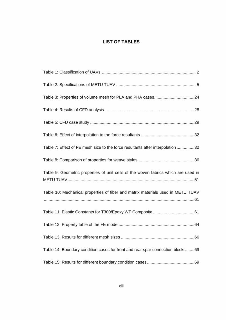
LIST OF TABLES

Table 1: Classification of UAVs ............................................................................... 2

Table 2: Specifications of METU TUAV ................................................................... 5

Table 3: Properties of volume mesh for PLA and PHA cases..................................24

Table 4: Results of CFD analysis ............................................................................28

Table 5: CFD case study ........................................................................................29

Table 6: Effect of interpolation to the force resultants .............................................32

Table 7: Effect of FE mesh size to the force resultants after interpolation ...............32

Table 8: Comparison of properties for weave styles ................................................36

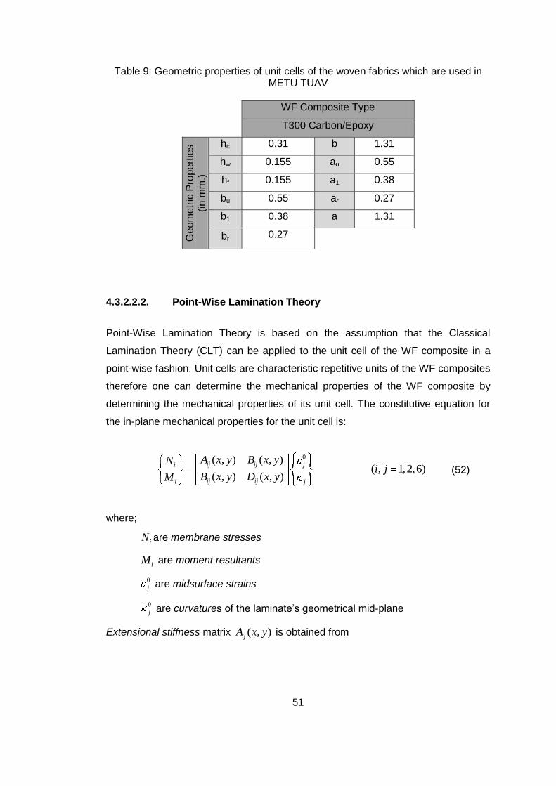
Table 9: Geometric properties of unit cells of the woven fabrics which are used in

METU TUAV ...........................................................................................................51

Table 10: Mechanical properties of fiber and matrix materials used in METU TUAV

...............................................................................................................................61

Table 11: Elastic Constants for T300/Epoxy WF Composite ...................................61

Table 12: Property table of the FE model ................................................................64

Table 13: Results for different mesh sizes ..............................................................66

Table 14: Boundary condition cases for front and rear spar connection blocks .......69

Table 15: Results for different boundary condition cases ........................................69

xiv

Table 16: Mechanical properties of isotropic materials used in METU TUAV ..........70

Table 17: Mechanical properties of 2D orthotropic materials ...................................70

Table 18: Comparison of results from unit cell analysis and values from literature ..71

Table 19: MoS value for front spar in PLA case ......................................................72

Table 20: MoS value for rear spar in PLA case .......................................................74

Table 21: MoS values for upper skin layers in PLA case .........................................75

Table 22: MoS values for lower skin layers in PLA case .........................................75

Table 23: MoS values for webs and ribs in PLA case .............................................77

Table 24: MoS value for front spar in PHA case .....................................................79

Table 25: MoS value for rear spar in PHA case ......................................................80

Table 26: MoS values for skin layers in PHA case ..................................................81

Table 27: MoS values for webs and ribs in PHA case .............................................83

Table 28: Comparison of peak stress and displacements for PLA and PHA cases .85

Table 29: First three normal modes and their frequency .........................................86

xv

LIST OF FIGURES

Figure 1: Examples for Different UAV Types: (a) Micro, (b) Mini, (c) Tactical, (d)

Medium Altitude Long Endurance (MALE), (e) High Altitude Long Endurance (HALE)

................................................................................................................................ 2

Figure 2: Three View of METU TUAV ...................................................................... 6

Figure 3: V-n diagram of METU TUAV ...................................................................10

Figure 4: E-Glass coated polystyrene foam used in the manufacturing of the METU

TUAV wing..............................................................................................................11

Figure 5: Male mold ready to be used as reference for female mold manufacturing 12

Figure 6: Covering the male mold with tool resin.....................................................13

Figure 7: Reinforcing the mold with woven E-glass woven fabric ............................13

Figure 8: Female wing molds ..................................................................................14

Figure 9: Manufacturing steps of the wing skins: (a) First e-glass layer, (b) Rohacell

foam layer, (c) Last e-glass layer, (d) Spar flanges in the lower skin .......................15

Figure 10: Positioning the spars ..............................................................................16

Figure 11: Allodized aluminum section of the rear spar ...........................................18

Figure 12: Hornbeam section of the front spar ........................................................19

Figure 13: Manufacturing of the spars: (a) Laying up the carbon woven fiber, ........20

xvi

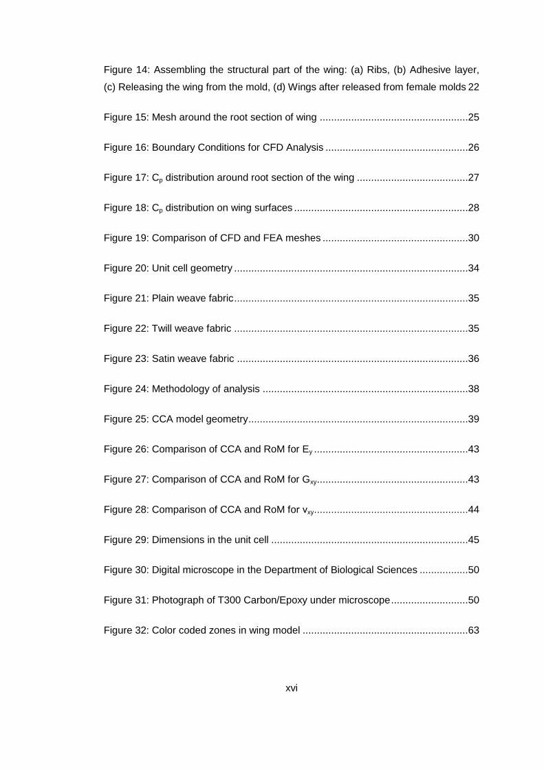
Figure 14: Assembling the structural part of the wing: (a) Ribs, (b) Adhesive layer,

(c) Releasing the wing from the mold, (d) Wings after released from female molds 22

Figure 15: Mesh around the root section of wing ....................................................25

Figure 16: Boundary Conditions for CFD Analysis ..................................................26

Figure 17: Cp distribution around root section of the wing .......................................27

Figure 18: Cp distribution on wing surfaces .............................................................28

Figure 19: Comparison of CFD and FEA meshes ...................................................30

Figure 20: Unit cell geometry ..................................................................................34

Figure 21: Plain weave fabric ..................................................................................35

Figure 22: Twill weave fabric ..................................................................................35

Figure 23: Satin weave fabric .................................................................................36

Figure 24: Methodology of analysis ........................................................................38

Figure 25: CCA model geometry .............................................................................39

Figure 26: Comparison of CCA and RoM for Ey ......................................................43

Figure 27: Comparison of CCA and RoM for Gxy .....................................................43

Figure 28: Comparison of CCA and RoM for νxy ......................................................44

Figure 29: Dimensions in the unit cell .....................................................................45

Figure 30: Digital microscope in the Department of Biological Sciences .................50

Figure 31: Photograph of T300 Carbon/Epoxy under microscope ...........................50

Figure 32: Color coded zones in wing model ..........................................................63

xvii

Figure 33: Detailed view of spar-body connection areas .........................................64

Figure 34: The detail of front spar connection in FE model .....................................65

Figure 35: Boundary conditions for wing connection blocks ....................................67

Figure 36: The finite element modeling of the tail boom ..........................................72

Figure 37: von Mises stress contours for front spar core material in PLA case .......73

Figure 38: von Mises stress contours for rear spar in PLA case ..............................74

Figure 39: von Mises stress contours for skin in PLA case .....................................76

Figure 40: von Mises stress contours for ribs and webs in PLA case ......................78

Figure 41: Deformation contour of the whole wing in PLA case ..............................78

Figure 42: von Mises stress contour for front spar in PHA case ..............................79

Figure 43: von Mises stress contour for rear spar in PHA case ...............................80

Figure 44: von Mises stress contours for skin in PHA case .....................................82

Figure 45: von Mises stress contours for ribs and webs in PHA case .....................84

Figure 46: Deformation contour of the whole wing in PHA case ..............................84

Figure 47: Mode shape for the first modal frequency (16.8Hz) ................................86

Figure 48: Mode shape for the second modal frequency (71.7 Hz) .........................87

Figure 49: Mode shape for the third modal frequency (84.5 Hz) ..............................87

Figure 50: The locations of applied force and monitored nodes ..............................88

Figure 51: Acceleration response of Node 658237 and Node 658553 ....................89

Figure 52: Locations of 75% semi span section and adjacent sections ...................92

xviii

Figure 53: The location of shear center at 0.75 semi-span ......................................93

Figure 54: Stitching of (a) stringer to skin, (b) rib to skin, (c) skin with integral spar

caps ........................................................................................................................96

Figure 55: Integral composite skin-stringer assembly .............................................97

Figure 56: Schematic of the VARTM process .........................................................98

Figure 57: VARTM setup before covering with vacuum bag ....................................98

Figure 58: VARTM setup with vacuum bag and resin lines .....................................98

Figure 59: Manufacturing steps of a cocured composite box ................................ 103

Figure 60: CAD model of the wing ........................................................................ 112

Figure 61: STEP file importing in GAMBIT. ........................................................... 113

Figure 62: Inner CFD domain................................................................................ 116

Figure 63: The whole CFD domain ....................................................................... 116

Figure 64: Boundary conditions for CFD analysis ................................................. 117

Figure 65: Selecting the solver properties in Fluent. ............................................. 118

Figure 66: Velocity inlet boundary condition .......................................................... 118

Figure 67: Opening the residual monitors ............................................................. 119

Figure 68: Solution control options ........................................................................ 119

Figure 69: Solution initialization ............................................................................ 119

Figure 70: Starting the iteration process in Fluent ................................................. 120

Figure 71: Writing the interpolation file .................................................................. 121

xix

Figure 72: Reading the interpolation file ................................................................ 121

Figure 73: Exporting the CFD data to MSC.Patran/Nastran .................................. 121

Figure 74: Flowchart of the procedure for interpolating CFD data into FE model .. 122

1

CHAPTER 1

INTRODUCTION AND LITERATURE REVIEW

1.1. Introduction to Tactical Unmanned Air Vehicles

Unmanned Aerial Vehicle (UAV) is a remotely piloted or self-piloted (autonomous)

aircraft that can carry cameras, sensors, communication equipments or other

payloads. They have been used in reconnaissance and intelligence-gathering roles

since the 1950s, and more challenging roles are envisioned, including combat

missions [1]. Nowadays they are also used in an increasing number of civil

applications such as meteorological measurements, disaster management and

maritime surveillance. UAVs are becoming popular day by day because of their low

cost, multi-role capabilities and ability of taking the risks from human in dangerous

missions.

UAVs are classified with respect to their mission profiles which are based on range,

endurance and cruise altitude. In general, endurance determines the fuel that is

carried, the chosen aerial communication technology has an impact on the

operational range and the cruise altitude affects the payload technology in

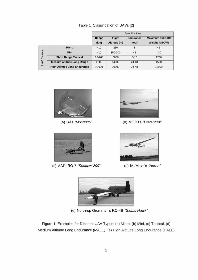
surveillance UAVs. According to Unmanned Vehicle Systems International [2] the

classification of UAVs is given in Table 1.

2

Table 1: Classification of UAVs [2]

Specifications

Range

(km)

Flight

Altitude (m)

Endurance

(hour)

Maximum Take-Off

Weight (MTOW) U

AV

Cla

sses

Micro <10 250 1 <5

Mini <10 150-300 <2 <30

Short Range Tactical 70-200 5000 6-10 1250

Medium Altitude Long Range >500 14000 24-48 1500

High Altitude Long Endurance >2000 20000 24-48 12000

(a) IAI‟s “Mosquito” (b) METU‟s “Güventürk”

(c) AAI‟s RQ-7 “Shadow 200” (d) IAI/Malat‟s “Heron”

(e) Northrop Grumman‟s RQ-4B “Global Hawk”

Figure 1: Examples for Different UAV Types: (a) Micro, (b) Mini, (c) Tactical, (d)

Medium Altitude Long Endurance (MALE), (e) High Altitude Long Endurance (HALE)

3

From military point of view, tactical UAVs are designed to support tactical

commanders with near-real-time imagery intelligence at ranges up to 200 kilometers

[1].

1.2. METU Tactical UAV (TUAV)

In Aerospace Engineering Department of Middle East Technical University (METU),

a UAV Research and Development project was started with the financial support of

State Planning Organization in 2005. The aim of this project was to build a mini and

a tactical UAV and establish the necessary infrastructure of a UAV research center

for future projects. The first output of the project, METU Mini UAV “Güventürk”, was

successfully manufactured and its flight tests were accomplished. A photograph of

Güventürk during a flight test is shown in Figure 1. The second outcome of the

project is a tactical UAV and this study is based on this tactical UAV platform. The

design of METU TUAV is complete and its first prototype is under construction.

4

CHAPTER 2

DESIGN AND MANUFACTURING OF THE METU TUAV

2.1. Design Features of METU TUAV

Most of the time, the attempt to create an aircraft design arises simply from the

need, and as a result the requirements of the end product are known. Looking at the

characteristics of previous examples would be the least time consuming and the

most efficient way to start a design process because it guarantees that the designer

has a number of ideas to develop therefore the outline is ready for a rough preview

of the conceptual design. This is how the design team of the METU TUAV including

the author of this thesis, started the conceptual design. Firstly a competitor study

was done and then by following the design steps of Raymer [3], the conceptual

design of the METU TUAV was finalized. To give the details of the conceptual

design process is beyond the scope of this thesis therefore only the results and

some parts related with structural design will be mentioned.

At the end of the conceptual design, the specifications of METU TUAV were decided

as shown in Table 2.

5

Table 2: Specifications of METU TUAV

Payload : Daylight / FLIR Camera (TBD)

Payload Weight : 20 kg

Wing Span : 4.3 m

Wing Aspect Ratio 8.39

Wing Taper Ratio 0.45

Length : 3 m

Maximum Take-off Weight : 105 kg

Cruise Velocity : 46 m/s

Stall Speed : 17 m/s

Operation Altitude : 3000 m

Operation Range : 150 km

Propulsion : 21 HP - Two Cycle Gasoline Engine

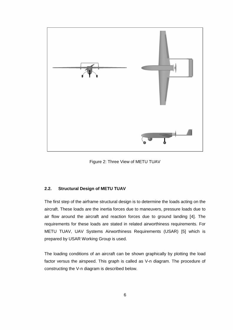
From the beginning of the conceptual design, CAD software CATIA V5 is used

extensively. Parametric design became the rule of thumb of the design team since it

decreases the man hour considerably. Once the initial 3D model of the METU TUAV

is done, critical parameters such as taper ratio, aspect ratio, reference wing surface

area etc are linked to it. This way when the critical parameters change during design

iterations 3D model can be updated in a very short time. The three view of the

METU TUAV can be seen in Figure 2. The computer aided design of the METU

TUAV was performed by the author of the thesis based on the conceptual design

parameters that came out after the work of the design team.

6

Figure 2: Three View of METU TUAV

2.2. Structural Design of METU TUAV

The first step of the airframe structural design is to determine the loads acting on the

aircraft. These loads are the inertia forces due to maneuvers, pressure loads due to

air flow around the aircraft and reaction forces due to ground landing [4]. The

requirements for these loads are stated in related airworthiness requirements. For

METU TUAV, UAV Systems Airworthiness Requirements (USAR) [5] which is

prepared by USAR Working Group is used.

The loading conditions of an aircraft can be shown graphically by plotting the load

factor versus the airspeed. This graph is called as V-n diagram. The procedure of

constructing the V-n diagram is described below.

7

a. Determination of stall speed, stallV :

In accelerating level flight conditions, lift produced by the aircraft is equal to

the product of the load factor and the weight of the aircraft.

n W L (1)

21

2L refn W V C S (2)

Therefore,

21

2

ref

L

Sn V C

W (3)

The curve constructed by using Equation (3) is a limiting condition which

represents the possible lift capability. It is also called the stall line.

For unaccelerated flight at stall conditions:

1 and stalln V V

max

(1 )

2stall g

ref L

WV

S C (4)

(1 ) 21.7 /stall gV m s for positive angle of attack

(1 ) 27.4 /stall gV m s for negative angle of attack

Values for (1 )stall gV and (1 )stall gV are different because the corresponding

maxLC values are different for positive and negative angles of attack [8].

For accelerated flight at stall conditions:

( ) (1 )stall ng stall gV V n (5)

b. Determination of positive and negative limit load factors:

According to “USAR.337a: Limit Maneuvering Load Factors” the positive limit

maneuvering load factor n may not be less than

8

10900

2.14536MTOW

(6)

where the maximum take-off weight is given in kg.

However, „USAR.337a: Limit Maneuvering Load Factors’ also specifies that

the load factor need not be more than 3.8. For the particular design Equation (6)

gives:

109002.1 4.45

105 4536n

Therefore, maximum positive load factor ()max(n ) is taken as 3.8.

According to USAR.337b, The negative limit maneuvering load factor may

not be less than 0.4 times the positive load factor.

Therefore, maximum positive load factor ()max(n ) is taken as 1.52.

According to USAR.333:, the velocity at the intersection of stall line and

max( )n line is the Design Maneuvering Speed, VA.

(3.8 ) (1 ) 3.8stall g stall gVA V V (7)

Thus, the design maneuvering speed is calculated as

42.3 / 82.2VA m s kts . This calculation assumes that the maximum lift coefficients

at 1g stall and at ng stall points are equal to each other.

The velocity at the intersection of stall line at negative angle of attacks and

max( )n line is the Negative Maneuvering Load Factor Speed, VG.

(1.52 ) (1 ) 1.52stall g stall gVG V V (8)

Thus, the negative maneuvering load factor speed is calculated as

33.8 / 65.7VG m s kts

9

c. Determination of design airspeeds:

According to USAR.335.a, VC is the Design Cruise Speed which may be

defined according to UAV operating requirements. In conceptual design

cruise speed is determined as:

46.3 / 90VC m s kts

According to USAR.335.b, Design Dive Speed, VD, may not be less than

1.25VC. In addition, according to Anderson [6], the high-speed limit velocity

is higher than the level flight maximum cruise velocity by a least factor of 1.2.

In conceptual design of METU TUAV, maximum cruise velocity was

calculated as 83m/s. Therefore, design dive speed is taken as:

max1.2VD V (9)

100 / 194VD m s kts

There is also a velocity that UAV should not exceed for safe operation. This

velocity is called as Never Exceed Speed, VNE. According to USAR.1505.1, never

exceed speed is given as

0.9VNE VD (10)

90 / 175VNE m s kts

After calculating necessary design speeds, V-n diagram of the METU TUAV is

constructed as shown in Figure 3.

10

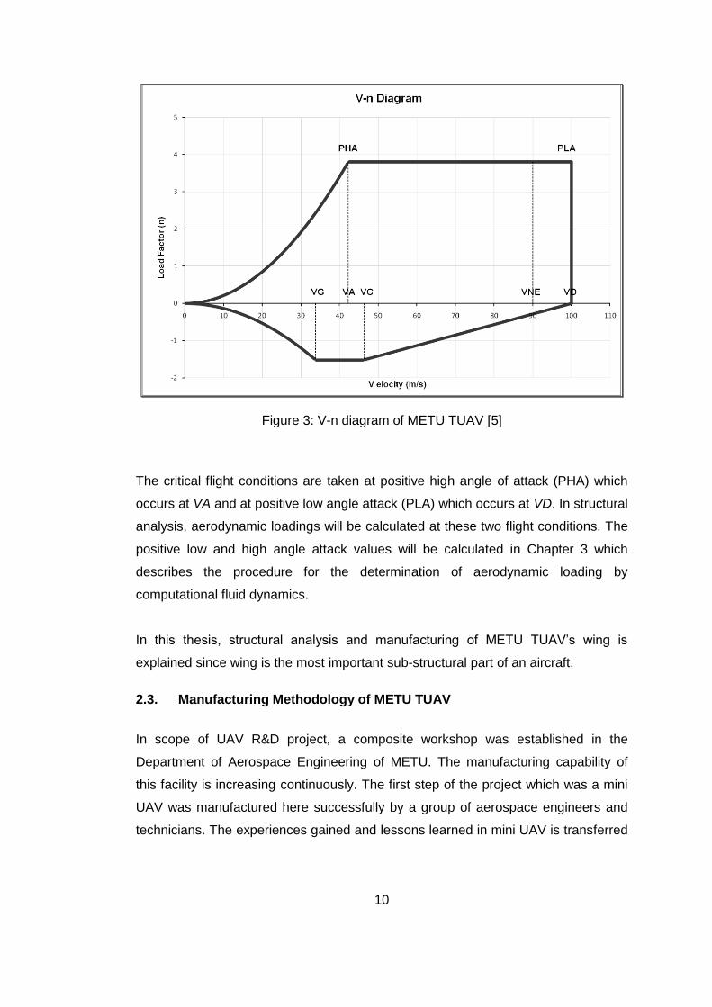
Figure 3: V-n diagram of METU TUAV [5]

The critical flight conditions are taken at positive high angle of attack (PHA) which

occurs at VA and at positive low angle attack (PLA) which occurs at VD. In structural

analysis, aerodynamic loadings will be calculated at these two flight conditions. The

positive low and high angle attack values will be calculated in Chapter 3 which

describes the procedure for the determination of aerodynamic loading by

computational fluid dynamics.

In this thesis, structural analysis and manufacturing of METU TUAV‟s wing is

explained since wing is the most important sub-structural part of an aircraft.

2.3. Manufacturing Methodology of METU TUAV

In scope of UAV R&D project, a composite workshop was established in the

Department of Aerospace Engineering of METU. The manufacturing capability of

this facility is increasing continuously. The first step of the project which was a mini

UAV was manufactured here successfully by a group of aerospace engineers and

technicians. The experiences gained and lessons learned in mini UAV is transferred

11

to the manufacturing activities of the tactical UAV. The manufacturing method used

in tactical UAV is similar to the method used in mini UAV manufacturing. The

manufacturing of composite airframe relies basically on the application of vacuum

bagging technique on the female molds. This technique is explained in detail in a

previous thesis study by Turgut [7]. Therefore a repetition of this work is not done in

this thesis. However, emphasis will be given to the differences in the manufacturing

methodology followed.

2.3.1. Preparation of Molds

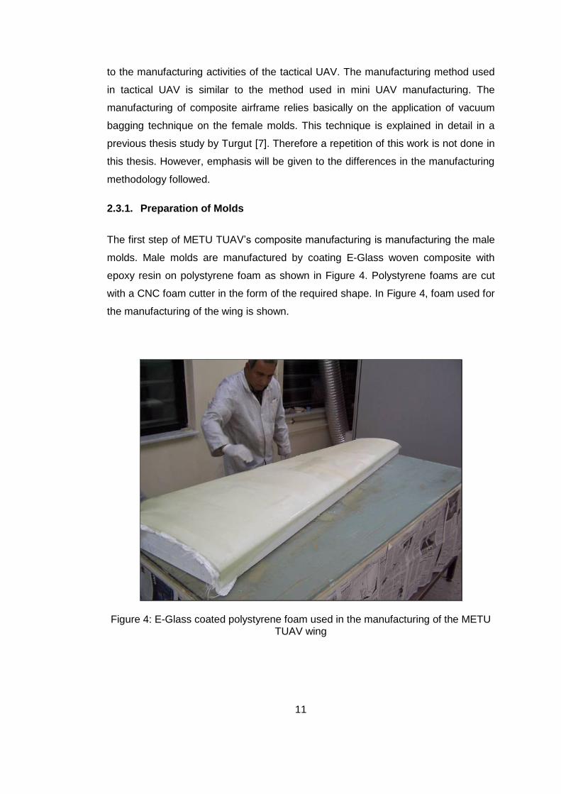
The first step of METU TUAV‟s composite manufacturing is manufacturing the male

molds. Male molds are manufactured by coating E-Glass woven composite with

epoxy resin on polystyrene foam as shown in Figure 4. Polystyrene foams are cut

with a CNC foam cutter in the form of the required shape. In Figure 4, foam used for

the manufacturing of the wing is shown.

Figure 4: E-Glass coated polystyrene foam used in the manufacturing of the METU TUAV wing

12

The female molds are manufactured by coating E-Glass woven composite with a

special laminate tool resin on male molds and reference surfaces. Figure 5 shows

the finished male model whose surfaces are used as the reference surfaces in

manufacturing of the female molds.

Figure 5: Male mold ready to be used as reference for female mold manufacturing

The main difference between the female molds of mini UAV and that of the tactical

UAV is the materials used in manufacturing. In mini UAV‟s female molds, the fiber

material is chopped fiber E-Glass and the resin material is polyester. Polyester

cures fast and exothermically. The generated heat during the curing process may

deform the mold if the heat cannot be transferred by means of ventilation. Also the

molds which are manufactured using this procedure cannot withstand high

temperatures. Because the chopped fiber-polyester composite material cannot

withstand thermal strains which affect the dimensional tolerances of work piece in

the mold. Therefore it is risky to use them in curing ovens where the molds may

deform and the final end product may lose geometric accuracy. In tactical UAV‟s

female molds, thick E-Glass woven tool fabric and a special laminate tool resin is

13

used as shown in Figure 6 and Figure 7. With the use of thick woven E-Glass woven

tool fabric and special tool resin, a stiffer mold with a better surface quality is

achieved. The finished female molds of METU TUAV‟s wing can be seen in Figure

8.

Figure 6: Covering the male mold with tool resin

Figure 7: Reinforcing the mold with woven E-glass woven fabric

14

(a) Side View (b) Top View

Figure 8: Female wing molds

2.3.2. Manufacturing of the Wing

Manufacturing of the wing is done in four steps.

1. Manufacturing of the skins

2. Manufacturing of the front and rear spars

3. Manufacturing of the ribs

4. Assembling all of the components

METU TUAV‟s composite parts are manufactured with vacuum bagging technique.

In all composite parts, Araldite LY 5052 epoxy is used as resin material. Skins are

composite sandwich structure having Rohacell 31A core material between e-glass

layers. Different from the manufacturing of the upper skin, in spar locations of lower

skin carbon fabric layer are added which will form the lower flanges of the spar later.

The manufacturing steps of the wing skins are shown in Figure 9. Figure 9d shows

the placement of the carbon fabric on the lower skin. The choice of lower skin for the

placement of carbon fabric to form the front and rear spar caps is due to the fact that

during flight the wing will be under up-bending resulting in tensile loads in the lower

skin for most of the time.

15

(a) (b)

(c) (d)

Figure 9: Manufacturing steps of the wing skins: (a) First e-glass layer, (b) Rohacell

foam layer, (c) Last e-glass layer, (d) Spar flanges in the lower skin

One lesson learned from METU mini UAV was to make the structural parts as

integrated as possible. The integrated manufacturing of composite parts has some

advantages like weight saving by reducing adhesive material and achieving better

structural integrity between the spar and the skin by the removing adhesive layer.

Therefore, in the manufacturing of the wing of the tactical UAV, the spars are not

simply adhesively bonded to the upper and lower skin after separate manufacturing

of the spars and upper and lower skins. The goal is to manufacture the spar cap-

lower skin connection by vacuum bagging of the spar fabrics, which will be laid over

the spar molds, with the lower skin and overlay the spar fabric extensions with the

16

carbon fabric strips that were already placed on the lower skin of the wing (Figure

9d) and cured under vacuum at 50°C in curing oven

Figure 10: Positioning the spars

After manufacturing of the lower skin, styrofoams are positioned in front and rear

spar locations on lower skin as shown in Figure 10. The spars are integrated to

lower skin because, as explained above, the lower skin is under tensile stress during

most of the flight times and the integrity of the spar and lower skin connection is

crucial. The styrofoams will be the male molds for spars and layers of carbon fabric

are laid on these permanent styrofoam molds. It is possible that ambient pressure

may deform the styrofoam molds when they are under vacuum. Therefore, before

positioning of the foam molds, they are coated on the web sides with one layer

carbon-epoxy to make them stiffer. This can be seen clearly in Figure 10. As shown

in Figure 10, spars are positioned on the carbon fabric strips which were placed

during the manufacturing of the lower skin of the wing. It should be noted that in the

current manufacturing method, lower wing skin and spar molds are manufactured

17

separately. However, as it will be explained in the following, spar fabrics which will

be placed over the strengthened spar molds will be coated with epoxy resin and

vacuum will be applied over the spar fabrics and thus the spar fabric extensions will

be cured on the lower skin carbon fabric strips which were placed over the lower

skin of the wing during the manufacturing of the lower skin of the wing. A better way

would be to manufacture spars and the lower skin in one vacuuming operation

integrally. However, in this method there is a possibility of distorting the position of

the spar molds during the vacuum bagging operation. Therefore, in order not to risk

the probable distortion of the wing spars during the vacuum bagging operation,

lower wing skin is manufactured first, and then spars are integrated to the lower skin

by a second vacuum bagging operation.

In the places near to the root of the wing styrofoams are replaced with different

materials. These sections of the spars should be stronger since the wing will be

attached to the fuselage from the ends of spars with bolts. In rear spar aluminum

7075-T6 is used as substitute material. Figure 11 shows the rear spar wing root

reinforcement. It is known that aluminum and carbon are not compatible materials to

be used together. The reason is the different electrochemical properties of these

materials. In an environment with an electrolyte such as humidity, the contact of

aluminum and carbon fiber results in galvanic corrosion of aluminum. To prevent the

corrosion, aluminum is electroplated with alodine and a thin e-glass epoxy layer is

laid between carbon and aluminum. Since both e-glass and epoxy are perfect

insulators, this layer will prevent aluminum from corrosion.

18

Figure 11: Allodized aluminum section of the rear spar

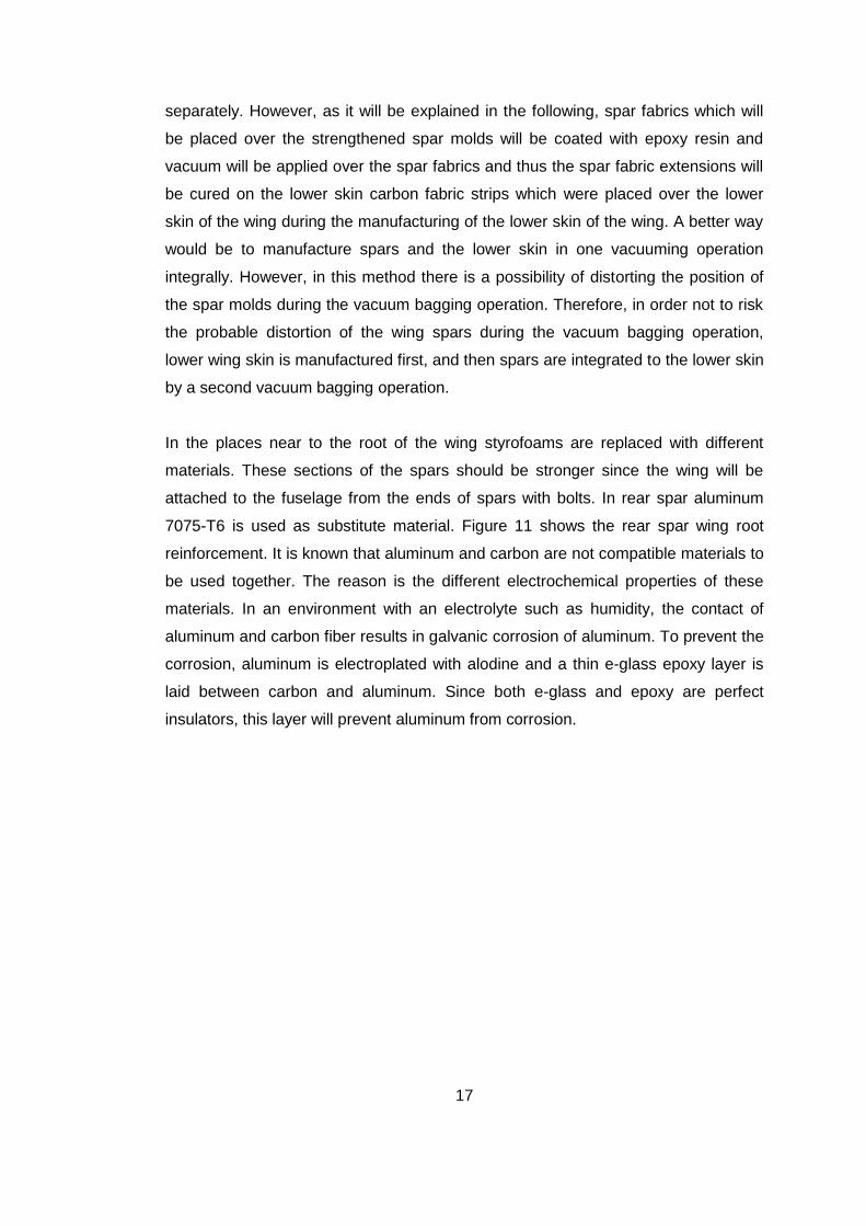
In front spar, laminated hornbeam wood is used as the reinforcement material at the

root, and this is shown in Figure 12. Hornbeam also called “ironwood”, is a very hard

wood and can give exceptional strength properties. Its ultimate strength in fiber

direction is 153MPa. The thickness of the hornbeam wood is composed of layers

hornbeam plies which are compacted to the required thickness. Layers of hornbeam

are adhesively joined with each other with epoxy resin.

19

Figure 12: Hornbeam section of the front spar

Figure 11 and Figure 12 show that the rear spar wing root ends at the end of the

wing, whereas, the root of the front spar extends outside the wing. With this

structural design, it was intended to place the front spar in a box which will be

connected to the fuselage such that the box and fuselage axes will be perpendicular

to each other. The spars were designed such that the front spar was perpendicular

to the chordline, but the rear spar does not intersect the chordline perpendicularly.

Therefore, the extension of the rear spar outside the wing would necessitate a

fuselage box which would have to be placed at an angle different from ninety

degrees with respect to the fuselage axis. In addition, it was decided not to make

any kinks along the length of the spars in order to prevent stress concentrations

associated with the kinks. Therefore, the rear spar should preserve its direction.

Thus, in the final design in order to eliminate the difficulties associated with the

assembly of the wing to the fuselage, it is decided to connect the rear spar to the

fuselage bulkhead on the rear spar side with two bolts through the aluminum

reinforcement placed at the root of the rear spar. On the other hand, the front spar

20

will be placed in a box structure which will be connected to the fuselage bulkhead at

the front spar side.

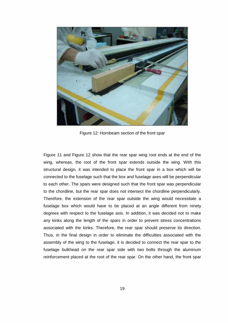
In the next step, woven carbon layers are laid on the strengthened spar molds and

wing root end reinforcements and final vacuum bagging is applied locally to the

spars along the full span of the wing. In this way spar and lower wing skin

connection is generated under vacuum eliminating the probable formation of voids

during the curing operation. The curing process is done in the curing oven at 50°C.

(a) (b)

(c)

Figure 13: Manufacturing of the spars: (a) Laying up the carbon woven fiber,

(b) Spars in vacuum bag, (c) Finished rear spar

21

The last major step of manufacturing of the wing is to close the upper skin on to the

integrated spar-rib-lower skin structure. Before this operation ribs are placed in the

required places along the span of the wing as shown in Figure 14a and Figure 14b.

Ribs are separately manufactured as a sandwich structure which consists of two

separate layers of hornbeam wood, center foam and carbon fabric layers between

the wood and foam material. Ribs are first connected to the lower skin by means E-

Glass fabric and epoxy resin along the lower edge of the rib which intersects with

the lower skin. After the ribs are fixed in their positions on the lower skin, the upper

edges of the ribs, which will face the upper skin of the wing, are trimmed and a close

match is obtained between the ribs and the upper skin. The match is frequently

checked by placing the upper skin over the lower skin assembly and checking the

gap between the spars and ribs with the upper skin. This process is an iterative

process and requires frequent checking of the gap after the upper skin is placed

over the lower skin assembly. It should be noted that the thickness of the adhesive

which will be placed over the spars and wing ribs has to be taken into account, and

therefore small gap has to be provided between the upper faces of the spar and the

ribs facing the upper skin and the upper skin itself. The upper skin is joined to the

other parts with structural adhesive as shown in Figure 14. The brown color material

in Figure 14b is a mixture of the adhesive and chopped wood particles. The

chopped wood particles increase the strength of the adhesive by serving as

discontinuous short fibers at random orientation. Assembly is completed by placing

the two parts of the female wing molds over each other and clamping the molds

along the circumference of the matching surfaces of the both parts of the female

molds. The assembly is left for cure for twelve hours. After the cure is complete, the

female molds are separated and the wing which usually remains in one part of the

female mold is taken out for final trimming, surface finishing and painting operation.

22

(a) (b)

(c) (d)

Figure 14: Assembling the structural part of the wing: (a) Ribs, (b) Adhesive layer,

(c) Releasing the wing from the mold, (d) Wings after released from female molds

23

CHAPTER 3

DETERMINATION OF AERODYNAMIC LOADING BY COMPUTATIONAL

FLUID DYNAMICS

3.1. Introduction

For structural analysis of a wing, it is necessary to find the loading on the wing. This

loading is due to aerodynamic forces coming from 3D pressure distribution on the

wing. The distribution of these aerodynamic forces acting on the wing can be found

either by experimental techniques using wind tunnel measurements or by means of

numerical methods using computational fluid dynamics (CFD) or by means of

empirical methods. Although the experimental techniques are the most accurate and

reliable method for determining these forces, their use is restricted by their high cost

and the limited availability of appropriate wind tunnels. On the other hand, numerical

methods are replacing wind tunnel tests because of their increasing accuracy in

determining the aerodynamic forces and moments acting on aircraft. With today‟s

very fast and modern computers it is possible to perform numerical wind tunnel

experiments in a very short time and with the precision of experimental results and

with very low cost. Engineering methods based on empirical tools also give very fast

results however their accuracy are not comparable to numerical techniques.

In this study, CFD method is used to calculate the flow field around the wing and the

resulting 3D pressure distribution acting on the wing. Then from this pressure

distribution the nodal forces are calculated and then they are exported into the finite

element program by means of interpolation from the CFD mesh to finite element

mesh. In this study, flow field computations are performed using the commercially

available CFD tool Fluent 6.2.16, and the structural analyses were performed by

MSC Patran/Nastran.

24

3.2. Generation of the Computational Mesh

The first step of the CFD calculation is to generate the computational mesh in the

flow field domain. The computational mesh is generated by a commercial package

program Gambit. First, the domain is divided into two sub-domains; inner and outer

domains, with variable grid spacings and intensities. The grid spacing in the inner

domain is much finer and contains ten times more elements than the outer domain.

The volume of the inner domain covers only 0.25% of the outer domain.

(Vinner=0.25%*Vouter) The domain is nested in such a way because the pressure

gradients are higher in the vicinity of the wing than the farfield zones. The CFD

mesh used is given in Figure 15. Two different volume meshes are generated for

cases PHA (Positive High Angle of Attack) and PLA (Positive Low Angle of Attack).

Model summary for both cases is tabulated in Table 3.

Table 3: Properties of volume mesh for PLA and PHA cases

AoA 0° AoA 14°

Number of Cells 2,951,886 2,814,039

Number of Nodes 514,007 490,929

For PHA angle of attack is set to 14° which is the stall angle of attack for the airfoil

profile of the wing. In PLA case, angle of attack is set to 0° which can be found from

the following calculations.

21

2L refn W V C S (11)

Therefore:

2

2L

ref

n WC

V S (12)

25

According to USAR.337a it is found that max( ) 3.8n and velocity is set to design

dive speed ( 100 /VD m s ). Inserting the rest of the variables in Equation (12)

yields to a lift coefficient of:

0.29LC

Although the lift coefficient of a wing is not identical to its airfoil‟s lift coefficient due

to 3D aerodynamic effects, at low angles of attack this discrepancy is negligible. The

corresponding angle of attack for 0.29Lc is 0° for NACA 63412 [8].

Figure 15: Mesh around the root section of wing

26

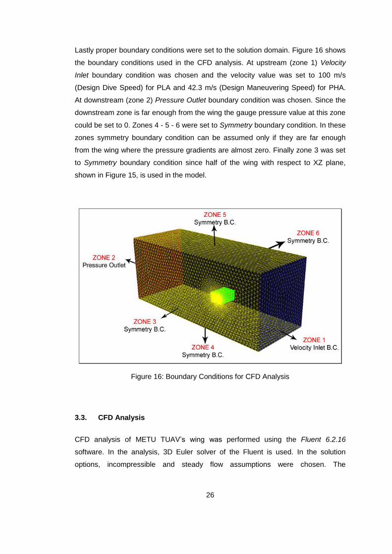
Lastly proper boundary conditions were set to the solution domain. Figure 16 shows

the boundary conditions used in the CFD analysis. At upstream (zone 1) Velocity

Inlet boundary condition was chosen and the velocity value was set to 100 m/s

(Design Dive Speed) for PLA and 42.3 m/s (Design Maneuvering Speed) for PHA.

At downstream (zone 2) Pressure Outlet boundary condition was chosen. Since the

downstream zone is far enough from the wing the gauge pressure value at this zone

could be set to 0. Zones 4 - 5 - 6 were set to Symmetry boundary condition. In these

zones symmetry boundary condition can be assumed only if they are far enough

from the wing where the pressure gradients are almost zero. Finally zone 3 was set

to Symmetry boundary condition since half of the wing with respect to XZ plane,

shown in Figure 15, is used in the model.

Figure 16: Boundary Conditions for CFD Analysis

3.3. CFD Analysis

CFD analysis of METU TUAV‟s wing was performed using the Fluent 6.2.16

software. In the analysis, 3D Euler solver of the Fluent is used. In the solution

options, incompressible and steady flow assumptions were chosen. The

27

incompressibility effects usually occur after Mach 0.3. In PLA case, the velocity is

the dive speed of the METU TUAV, 100 m/s (Mach 0.3) therefore incompressible

flow assumption is deemed to be convenient.

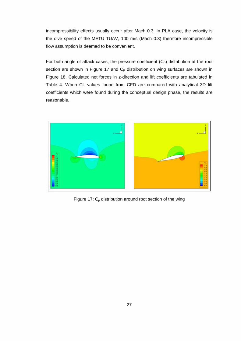
For both angle of attack cases, the pressure coefficient (CP) distribution at the root

section are shown in Figure 17 and CP distribution on wing surfaces are shown in

Figure 18. Calculated net forces in z-direction and lift coefficients are tabulated in

Table 4. When CL values found from CFD are compared with analytical 3D lift

coefficients which were found during the conceptual design phase, the results are

reasonable.

Figure 17: Cp distribution around root section of the wing

28

Figure 18: Cp distribution on wing surfaces

Table 4: Results of CFD analysis

AoA = 0o AoA = 14o

Net Force in z (N) 1737 1410

CL from CFD 0.258 1.19

CL theoretical [6] 0.261 1.39

The differences between the theoretical and computational CL values can be

attributed to the assumptions made in both methods of calculations. First of all in

CFD calculations, the velocities at which the solutions are done are determined from

29

V-n diagram. When constructing the V-n diagram, airfoil data is used and it does not

include the 3D effects. Secondly, the theoretical CL values are not exact and they

are not found from exact formulas. Nevertheless in terms of structural analysis, it is

the distribution of the pressure around the wing which is important but not the

resultant integrated forces found from the CFD computations. As long as the

pressure distribution found from CFD reflects the actual case, the net forces can be

scaled up to the desired value in finite element program.

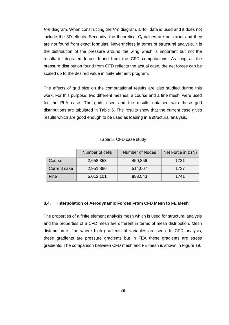
The effects of grid size on the computational results are also studied during this

work. For this purpose, two different meshes, a course and a fine mesh, were used

for the PLA case. The grids used and the results obtained with these grid

distributions are tabulated in Table 5. The results show that the current case gives

results which are good enough to be used as loading in a structural analysis.

Table 5: CFD case study

Number of cells Number of Nodes Net Force in z (N)

Course 2,658,358 450,856 1731

Current case 2,951,886 514,007 1737

Fine 5,012,101 888,543 1741

3.4. Interpolation of Aerodynamic Forces From CFD Mesh to FE Mesh

The properties of a finite element analysis mesh which is used for structural analysis

and the properties of a CFD mesh are different in terms of mesh distribution. Mesh

distribution is fine where high gradients of variables are seen. In CFD analysis,

these gradients are pressure gradients but in FEA these gradients are stress

gradients. The comparison between CFD mesh and FE mesh is shown in Figure 19.

30

Figure 19: Comparison of CFD and FEA meshes

31

In CFD analysis the forces are calculated at the nodes of elements. Therefore these

forces should be transferred to FE mesh in order to perform the structural analyses.

In this thesis, Fluent‟s interpolate option was used to transfer these nodal forces to

FE mesh. In order to do this, firstly, a surface mesh on the wing surface is created in

Gambit, which is the identical to the mesh as used in finite element analyses. Finer

mesh was used in high stress gradient areas, i.e. near to the root of wing. Using this

surface mesh a 3D volume mesh was generated again in the whole computational

domain. The geometrical boundaries of this 3D mesh need to be the same as the

boundaries of the CFD mesh which is used to determine the pressure distribution. At

this step Fluent can perform interpolation between these two 3D domains. Thus, grid

forces calculated in the CFD mesh can be interpolated to the mesh which will be

used for the structural analysis.

The whole interpolation process is described in Appendix A including the generation

of the wing geometry, mesh generation by Gambit to be used for interpolation

purposes and analysis performed by Fluent to accomplish the interpolation.

Appendix A is prepared by presenting snapshots from the related menus of the

different analysis tools to make the process more descriptive.

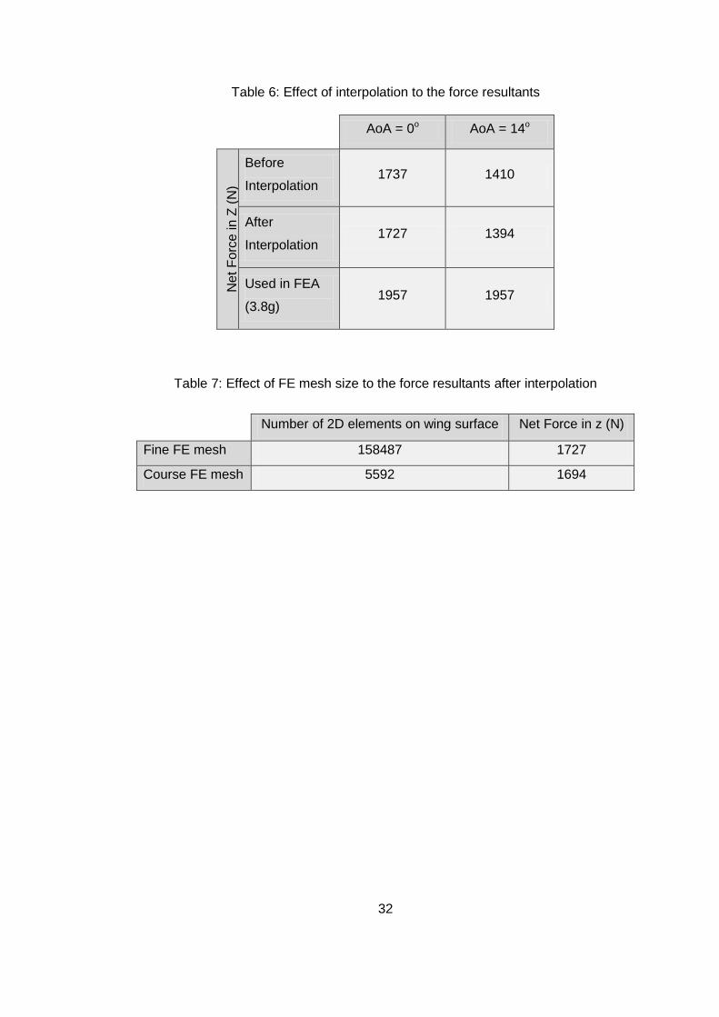
After the interpolation, the surface meshes together with the nodal forces are

exported as MSC. Nastran *.bdf files which are the input files of MSC. Nastran. After

this interpolation process, the net forces acting on the wing were found to be not the

same as the net forces before interpolation. The net z-force comparison before and

after the interpolation procedure is given in Table 6. As it can be seen from Table 6,

the difference in the net force in the z- direction before and after the interpolation is

very small and the interpolation process is considered to be satisfactory. As

mentioned before, the force resultants can be shifted up to the desired value as long

as the pressure distribution is accurate. The finite element analysis for PHA and

PLA, are conducted at 3.8g and the results are indicated in Table 6.

The effect of the FE mesh size to interpolation is also investigated and the results

are tabulated in Table 7.

32

Table 6: Effect of interpolation to the force resultants

AoA = 0o AoA = 14o

Ne

t F

orc

e in

Z (

N)

Before

Interpolation 1737 1410

After

Interpolation 1727 1394

Used in FEA

(3.8g) 1957 1957

Table 7: Effect of FE mesh size to the force resultants after interpolation

Number of 2D elements on wing surface Net Force in z (N)

Fine FE mesh 158487 1727

Course FE mesh 5592 1694

33

CHAPTER 4

MECHANICAL PROPERTIES OF WOVEN FABRIC COMPOSITES

4.1. Introduction

2D Composite fabrics are divided into three groups in terms of fiber orientation and

techniques that keeps the fibers together. These are unidirectional, woven, and

multiaxial. For unidirectional (UD) fabrics, the fibers go through in one direction

usually 0° direction which also called the warp direction. Multiaxial fabrics consist of

one or more layers of long fibers held in place by a secondary non-structural

stitching tread. The main fibers can be any of the structural fibers available in any

combination [9]. Woven fabrics (WF) are made of by twisting fibers in warp (0°) and

weft (90°) directions in a systematic pattern and weave style.

Woven fabrics have some advantages over unidirectional fabrics. They have

superior damage tolerance. WF composites provide more balanced properties in the

fabric plane and higher impact resistance than UD composites. The interlacing of

yarns provides higher out-of plane strength which can take up the secondary loads

due to load path eccentricities, local buckling etc [10]. Also composite manufacturing

using WF is easier since their handling is easier and they adapt to surfaces better

than UD fabrics. Apart from these advantages, WF composites have inferior in-plane

stiffness and strength properties compared to UD ones because of the undulation of

yarns.

The use of WF composites has been mostly limited to the secondary structures

because of lack of understanding on their mechanical behavior [11]. Classical

Laminate Theory (CLT) is widely used to calculate the elastic properties of the flat

composite plies which have homogenous fiber distribution and arrangement. For WF

composites, the fibers are concentrated in yarns which results a non-homogenous

34

fiber distribution. Therefore CLT should be modified in order to find elastic properties

of WF composites.

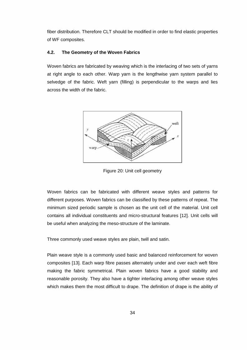
4.2. The Geometry of the Woven Fabrics

Woven fabrics are fabricated by weaving which is the interlacing of two sets of yarns

at right angle to each other. Warp yarn is the lengthwise yarn system parallel to

selvedge of the fabric. Weft yarn (filling) is perpendicular to the warps and lies

across the width of the fabric.

Figure 20: Unit cell geometry

Woven fabrics can be fabricated with different weave styles and patterns for

different purposes. Woven fabrics can be classified by these patterns of repeat. The

minimum sized periodic sample is chosen as the unit cell of the material. Unit cell

contains all individual constituents and micro-structural features [12]. Unit cells will

be useful when analyzing the meso-structure of the laminate.

Three commonly used weave styles are plain, twill and satin.

Plain weave style is a commonly used basic and balanced reinforcement for woven

composites [13]. Each warp fibre passes alternately under and over each weft fibre

making the fabric symmetrical. Plain woven fabrics have a good stability and

reasonable porosity. They also have a tighter interlacing among other weave styles

which makes them the most difficult to drape. The definition of drape is the ability of

35

a fabric to fold on itself and to conform to the shape of the article it covers [14]. This

disadvantage may cause difficulties in manufacturing during preparing the preform

or lay-up process. Also the high level of fibre crimp results inferior mechanical

properties compared with the other weave styles.

Figure 21: Plain weave fabric

In Twill weave style one or more warp fibres varyingly weave over and under two or

more weft fibres in a regular recurring way. With little sacrificing in the stability they

provide better wet-out and drape properties than plain weave style. Also fibre crimp

levels are lower which results better mechanical properties and smoother surfaces.

Figure 22: Twill weave fabric

36

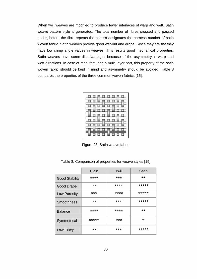
When twill weaves are modified to produce fewer interlaces of warp and weft, Satin

weave pattern style is generated. The total number of fibres crossed and passed

under, before the fibre repeats the pattern designates the harness number of satin

woven fabric. Satin weaves provide good wet-out and drape. Since they are flat they

have low crimp angle values in weaves. This results good mechanical properties.

Satin weaves have some disadvantages because of the asymmetry in warp and

weft directions. In case of manufacturing a multi layer part, this property of the satin

woven fabric should be kept in mind and asymmetry should be avoided. Table 8

compares the properties of the three common woven fabrics [15].

Figure 23: Satin weave fabric

Table 8: Comparison of properties for weave styles [15]

Plain Twill Satin

Good Stability **** *** **

Good Drape ** **** *****

Low Porosity *** **** *****

Smoothness ** *** *****

Balance **** **** **

Symmetrical ***** *** *

Low Crimp ** *** *****

37

4.3. Elastic Constants of Woven Fabrics

4.3.1. Introduction to Modeling of Elastic Analysis of Woven Fabrics

Concentrated fibers in the yarn makes woven fabrics highly non-homogenous. As a

result the fibre volume fraction is distributed in the weave heterogeneously. Since

the fibre volume fraction affects the stiffness of the composite material significantly,

it is important to construct a proper material model in order to find the elastic

properties. In literature there are three different approaches that deal with elastic

properties of woven fabrics.

1. The Elementary Models

2. Numerical Methods

3. Laminate Theory

The elementary models give crude estimation of elastic properties of WF

composites. Modeling WF composite as a laminate of UD laminae is an example for

elementary model.

Numerical models consist of modeling the unit cell geometry and analyzing this

geometry using mostly finite element method. Numerical models can give detailed

information about stress and strain inside the unit cell but they are complex models

and for different woven fabric new geometry and mesh should be constructed in

order to predict the mechanical properties of the WF composite.

Another approach to predict the elastic properties of a WF lamina is using analytical

methods based on classical laminate theory. Firstly Halpin et al. [16] used laminate

analogy by modeling the weft and warp yarn as angle-ply laminates and combine

them to form symmetrical laminates. Ishikawa and Chou [17-18-19] have developed

three models called mosaic model, crimp model and bridging model. In the mosaic

model a woven composite is idealized as an assemblage of pieces of asymmetric

cross-ply laminates. The crimp model is developed in order to consider the

continuity and undulations of the fiber in a fabric composite. Lastly in bridging model

the interactions between an undulated region and its surrounding regions with

38

straight threads were considered [20]. All these models are one dimensional models

and these models are further improved by Naik and Shembekar [10]. Naik and

Shembekar extended Ishikawa and Chou‟s crimp model to 2D by considering

undulations in both warp and weft directions. Falzon et.al [21] has presented a

similar model but this time considering continuity of the fibre structure which was

neglected before.

4.3.2. Material Model of the Woven Fabrics Used in METU TUAV

In order to make the finite element analysis of the METU TUAV, material properties

should be found. Since it is not always possible to find the elastic properties of the

woven composite fabrics, in this thesis elastic properties were found via analysis.

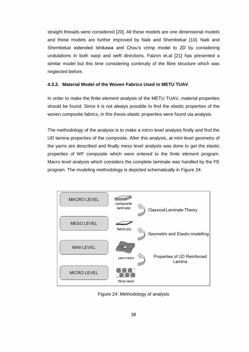
The methodology of the analysis is to make a micro level analysis firstly and find the

UD lamina properties of the composite. After this analysis, at mini level geometry of

the yarns are described and finally meso level analysis was done to get the elastic

properties of WF composite which were entered to the finite element program.

Macro level analysis which considers the complete laminate was handled by the FE

program. The modeling methodology is depicted schematically in Figure 24.

Figure 24: Methodology of analysis

39

4.3.2.1. Micro Level Analysis

In analytical method developed to analyze the WF composites, yarns can be taken

as equivalent UD composites. In the literature there are various methods to

calculate UD elastic properties from fibre volume fraction and mechanical properties

of fibre and resin. The simplest and the most known method is the Rule of Mixtures.

It gives good predictions in the fibre direction underestimates the transverse

properties of the composite material. There are also methods of Chamis, Puck,

Halpin-Tsai, Christensen and Hashin.

Among all these methods only Hashin‟s model admits anisotropy in the fibers

themselves; all the other models assume the fibers and resin are separately

isotropic. Assuming glass fibers are isotropic is very plausible. But the anisotropy in

common carbon fibers is substantial and Hashin's model should then be preferred

[22].

Hashin‟s model which is also known as Composite Cylinder Assemblage (CCA)

model [23,24], considers a collection of composite cylinders, each with a circular

fiber core in a concentric hollow matrix cylinder. The matrix and fiber volume

fractions are assumed to be same in each composite cylinder.

Figure 25: CCA model geometry

40

In the CCA model, the transverse bulk modulus of the UD lamina is given by [23,24]:

( )(1 ) ( )

( )(1 ) ( )

m f m f m m

TT f TT f

f m m m

TT f TT f

k k G V k k G Vk

k G V k G V (13)

with,

241 1 4f

LT

f f f f

TT L Tk G E E

(14)

241 1 4m

LT

m m m m

TT L Tk G E E (15)

The longitudinal modulus is given by [23,24],

24( )

1

f m

LT LT m ff m

L L f L mfm

f m m

TT

V VE E V E V

VV

k k G

(16)

In-plane poisson‟s ratio and in-plane shear modulus are given by [23,24],

( )(1/ 1/ )

1

f m m f

LT LT f mf m

LT LT f LT mfm

f m m

TT

k k V VV V

VV

k k G

(17)

(1 )

(1 )

m f

LT m LT fm

LT LT m f

LT f LT m

G V G VG G

G V G V (18)

The bounds for shear modulus transverse/transverse are given by [23,24],

The lower bound:

( )

21

2

fm

TT TT m m

TT m

f m m m mTT TT TT TT

VG G

k G V

G G G k G

(19)

41

The bounds for shear modulus transverse/transverse are given by [23,24],

The upper bound:

1

( )2 2

1

3

11

31

1

fm

TT TT

mf

f

VG G

VV

V

(20)

When,

f m

TT TTG G and f mk k

and,

( )

21

2

fm

TT TT m m

TT m

f m m m mTT TT TT TT

VG G

k G V

G G G k G

(21)

1

( )2 2

1

3

1

11

31

fm

TT TT

mf

f

VG G

VV

V

(22)

When,

f m

TT TTG G and f mk k

Here,

1 2

21 (23)

1

1 (24)

12

m

m m

TT

k

k G (25)

42

22

f

f f

TT

k

k G (26)

f

TT

m

TT

G

G (27)

1m fV V (28)

The bounds of TE are given by [23,24],

( )

( )

( )

4 TT

T

TT

kGE

k mG (29)

where,

241 LT

L

km

E (30)

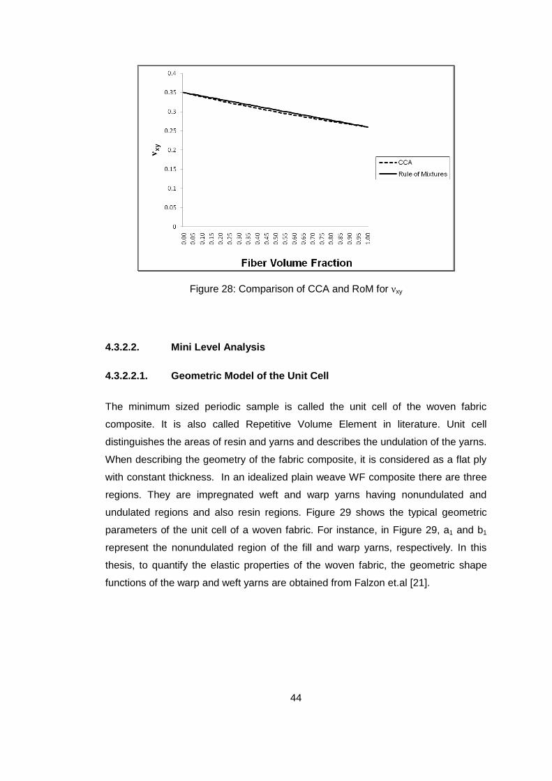
One can see how Rule of Mixtures underestimates the transverse properties of a

composite material by plotting the results versus fiber volume fraction. The following

example is for T300 Carbon / Araldite LY5052.

43

Figure 26: Comparison of CCA and RoM for Ey

Figure 27: Comparison of CCA and RoM for Gxy

44

Figure 28: Comparison of CCA and RoM for νxy

4.3.2.2. Mini Level Analysis

4.3.2.2.1. Geometric Model of the Unit Cell

The minimum sized periodic sample is called the unit cell of the woven fabric

composite. It is also called Repetitive Volume Element in literature. Unit cell

distinguishes the areas of resin and yarns and describes the undulation of the yarns.

When describing the geometry of the fabric composite, it is considered as a flat ply

with constant thickness. In an idealized plain weave WF composite there are three

regions. They are impregnated weft and warp yarns having nonundulated and

undulated regions and also resin regions. Figure 29 shows the typical geometric

parameters of the unit cell of a woven fabric. For instance, in Figure 29, a1 and b1

represent the nonundulated region of the fill and warp yarns, respectively. In this

thesis, to quantify the elastic properties of the woven fabric, the geometric shape

functions of the warp and weft yarns are obtained from Falzon et.al [21].

45

Figure 29: Dimensions in the unit cell

Warp Direction:

1( )2

cht y

: 0y b (31)

2 1

( )

2

( )( ) 1 sin ( )

2 2 2

( )

2

f w

f w f

u

w f

h h

h h ht y y b

b

h h

1

1 1

1

: 0

:

:

u

u

y b

y b b b

y b b b

(32)

3 1

( )

2

( )( ) 1 sin ( )

2 2 2

( )

2

w f

w f f

u

w f

h h

h h ht y y b

b

h h

1

1 1

1

: 0

:

:

u

u

y b

y b b b

y b b b

(33)

46

2 1

4 1

1( ) 1 sin

2 2

( ) sin ( )2( )

( )

2

f rr

u

r

u r

w f

h bt b b

b

t y y b bb b

h h

1 1

1

:

:

r u

u

y b b b b

y b b b

(34)

5 3 1

1

( )

2

1( ) ( ) 1 sin

2 2

sin ( )2( ) 2

w f

f ru r

u

u r

h h

h bt y t b b b

b

y bb b

1

1 1

: 0

: u r

y b

y b b b b

(35)

6( )2

cht y (36)

In equations (31) to (36), the main assumption is the sinusoidal variation of the warp

and fill yarns in a unit cell. In Figure 29 and equations (31) to (36) the geometric

parameters are defined as:

bu is the undulation length of the warp yarn

b1 is the nonundulated length of the warp yarn

b is the warp length of the unit cell

hf is the maximum thickness of the weft yarn

hw is the maximum thickness of the warp yarn

hc is the overall thickness of the composite layer

Crimp angle for warp yarn is defined as [21]:

1 3( )( ) tanw

dt yy

dy (37)

47

1

0

cos ( )2 2

0

f

u u

hy b

b b

1

1 1

1

: 0

:

:

u

u

y b

y b b b

y b b b

(38)

Weft Direction:

For the region 10 u ry b b b the shape functions are given as [21]:

1 1( , ) ( )h x y t y : 0x a (39)

5

5 32 5

1

( )

( ( ) ( ))( , ) ( )

2

1 sin ( )2u

t y

t y t yh x y t y

x aa

1

1

: 0

: / 2

x a

x a a

(40)

3

5 33 3

1

( )

( ( ) ( ))( , ) ( )

2

1 sin ( )2u

t y

t y t yh x y t y

x aa

1

1

: 0

: / 2

x a

x a a

(41)

2 1

3 1 1

5 353 2

( ) : 0

( , ) 1 sin ( )2( ) 2

( ) ( )( , ) ( ) ( )

2

u r

u r

t y x a

h a a a y x aa a

t y t yh x yt y t y

1 1

1 1 sin :

2

ru r

u

ax a a a a

a

(42)

48

6 6( , ) ( )h x y t y : 0 / 2x a (43)

In Figure 29 and Equations (39) to (43) the geometric parameters are defined as:

au is the undulation length of the weft yarn

a1 is the nonundulated length of the weft yarn

a is the weft length of the unit cell

For the region 1 / 2u rb b b y b the shape functions are given as [21]:

1 1( , ) ( )h x y t y : 0x a (44)

3

5 1 33 3

1

( )

( ( ) ( ) ( ))( , ) ( )

2

1 sin ( )2 ( ) 2

u r

u

t y

t b b b t y yh x y t y

x aa y

1

1

: 0

: / 2

x a

x a a

(45)

2

3 1

5 1

3 2

5 1 3

( )

( , )

( , ) sin ( )2( ) 2

( ) ( )

( ) ( ) ( )

2

( ) 11 sin

2 ( ) 2

u r

u r

u r

u r

u

t y

h a a a y

h x y x aa a

t y t y

t b b b t y y

a a

a y

1

1 1

: 0

: u r

x a

x a a a a

(46)

6 6( , ) ( )h x y t y : 0x a (47)

49

where

5 1 3 1( ) ( ( ) ( ) sin ( )2

u r u r

u r

y t b b b t y b b b yb b

(48)

and

1( ) sin ( )2 2

ur u r

u r

ay a b b b y

b b (49)

Crimp angle for weft yarn is defined as [21]:

1 3( )( ) tanw

dh yy

dy (50)

5 31

( ( ) ( ))cos ( )

2 2

0

u

t y t yx a

a

1

1 1

: 0

: u r

y b

y b b b b

(51)

Using the shape functions given above the geometric model of the WF composite

used in METU TUAV was constructed. First of all, the geometric parameters of the

woven carbon fiber/epoxy used in the manufacturing of the wing were obtained by

digital microscope photography in the Department of Biological Sciences in METU.

The digital microscope is shown in Figure 30 and taken photograph for

graphite/epoxy composite is shown in Figure 31.

50

Figure 30: Digital microscope in the Department of Biological Sciences

Figure 31: Photograph of T300 Carbon/Epoxy under microscope

According to measurements, the geometric parameters are tabulated in Table 9.

The symbols corresponding to the lengths in unit cell can be recalled from Figure

29.

51

Table 9: Geometric properties of unit cells of the woven fabrics which are used in METU TUAV

WF Composite Type

T300 Carbon/Epoxy

Ge

om

etr

ic P

ropert

ies

(in

mm

.)

hc 0.31 b 1.31

hw 0.155 au 0.55

hf 0.155 a1 0.38

bu 0.55 ar 0.27

b1 0.38 a 1.31

br 0.27

4.3.2.2.2. Point-Wise Lamination Theory

Point-Wise Lamination Theory is based on the assumption that the Classical

Lamination Theory (CLT) can be applied to the unit cell of the WF composite in a

point-wise fashion. Unit cells are characteristic repetitive units of the WF composites

therefore one can determine the mechanical properties of the WF composite by

determining the mechanical properties of its unit cell. The constitutive equation for

the in-plane mechanical properties for the unit cell is:

0( , ) ( , )

( , ) ( , )

ij iji j

ij iji j

A x y B x yN

B x y D x yM ( , 1,2,6)i j (52)

where;

iN are membrane stresses

iM are moment resultants

0

j are midsurface strains

0

j are curvatures of the laminate‟s geometrical mid-plane

Extensional stiffness matrix ( , )ijA x y is obtained from

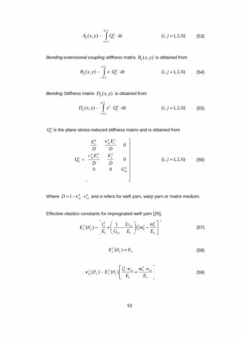
52

/2

/2

( , )

h

ij ij

h

A x y Q dz ( , 1,2,6)i j (53)

Bending-extensional coupling stiffness matrix ( , )ijB x y is obtained from

/2

/2

( , )

h

ij ij

h

B x y z Q dz ( , 1,2,6)i j (54)

Bending Stiffness matrix ( , )ijD x y is obtained from

/2

2

/2

( , )

h

ij ij

h

D x y z Q dz ( , 1,2,6)i j (55)

ijQ is the plane stress-reduced stiffness matrix and is obtained from

0

0

0 0

xy xx

xy x y

ij

xy

EE

D D

E EQ

D D

G

( , 1,2,6)i j (56)

Where 1 xy yxD and α refers for weft yarn, warp yarn or matrix medium.

Effective elastics constants for impregnated weft yarn [25],

14 4

2 213

1 13 1 3

21( )f

x f

l mE l m

E G E E (57)

2( )f

y fE E (58)

2 2

12 32

1 3

( ) ( )f f

xy f x f

l mE

E E (59)

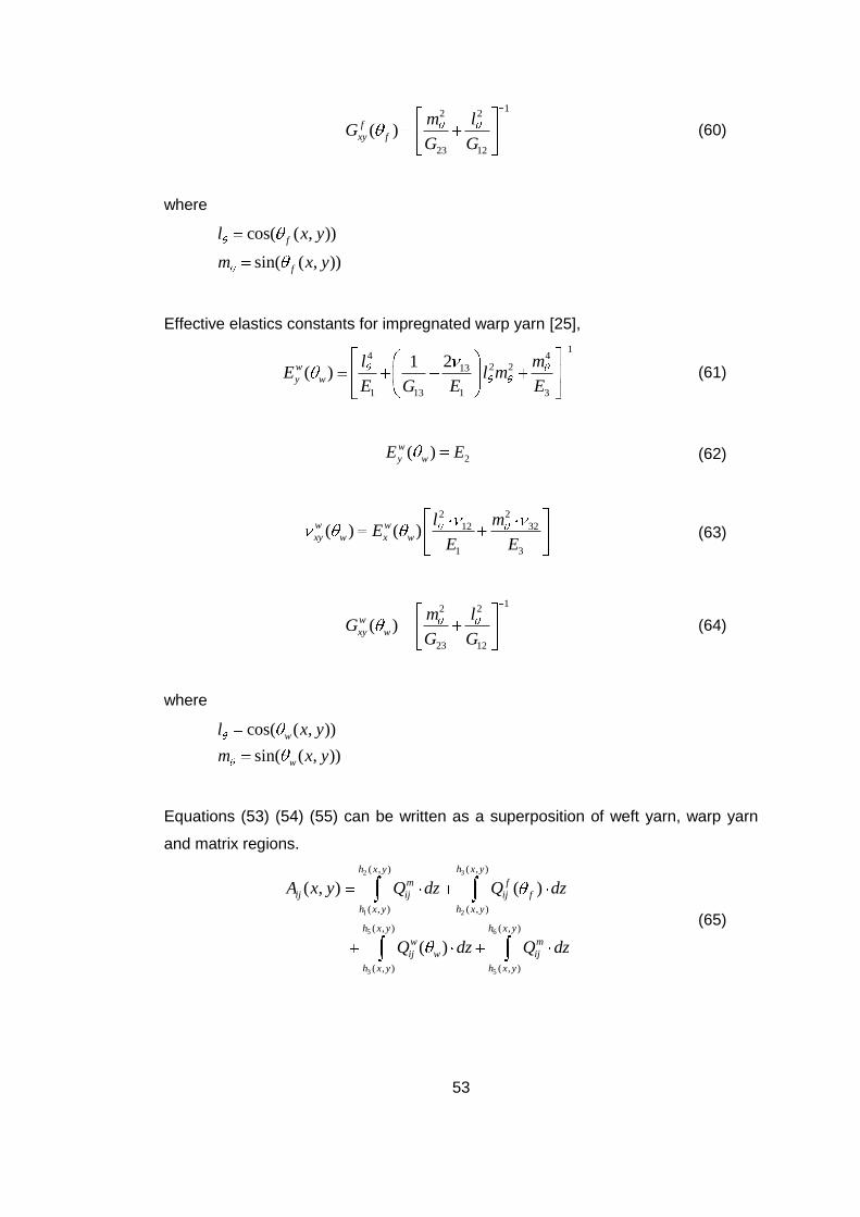
53

12 2

23 12

( )f

xy f

m lG

G G (60)

where

cos( ( , ))

sin( ( , ))

f

f

l x y

m x y

Effective elastics constants for impregnated warp yarn [25],

14 4

2 213

1 13 1 3

21( )w

y w

l mE l m

E G E E (61)

2( )w

y wE E (62)

2 2

12 32

1 3

( ) ( )w w

xy w x w

l mE

E E (63)

12 2

23 12

( )w

xy w

m lG

G G (64)

where

cos( ( , ))

sin( ( , ))

w

w

l x y

m x y

Equations (53) (54) (55) can be written as a superposition of weft yarn, warp yarn

and matrix regions.

32

1 2

5 6

3 5

( , )( , )

( , ) ( , )

( , ) ( , )

( , ) ( , )

( , ) ( )

( )

h x yh x y

m f

ij ij ij f

h x y h x y

h x y h x y

w m

ij w ij

h x y h x y

A x y Q dz Q dz

Q dz Q dz

(65)

54

32

1 2

5 6

3 5

( , )( , )

( , ) ( , )

( , ) ( , )

( , ) ( , )

( , ) ( )

( )

h x yh x y

m f

ij ij ij f

h x y h x y

h x y h x y

w m

ij w ij

h x y h x y

B x y Q z dz Q z dz

Q z dz Q z dz

(66)

32

1 2

5 6

3 5

( , )( , )

2 2

( , ) ( , )

( , ) ( , )

2 2

( , ) ( , )

( , ) ( )

( )

h x yh x y

m f

ij ij ij f

h x y h x y

h x y h x y

w m

ij w ij

h x y h x y

D x y Q z dz Q z dz

Q z dz Q z dz

(67)

For region 10 u ry b b b and

10 u rx a a a ,

3 2 5 3

2 1 6 5

( , ) ( ) ( , ) ( , ) ( ) ( , ) ( , )

( , ) ( , ) ( , ) ( , )

f w

ij ij f ij w

m

ij

A x y Q h x y h x y Q h x y h x y

Q h x y h x y h x y h x y (68)

2 2 2 2

3 2 5 3

2 2 2 2

2 1 6 5

( ) ( )( , ) ( , ) ( , ) ( , ) ( , )

2 2

( , ) ( , ) ( , ) ( , )2

f w

ij f ij w

ij

m

ij

Q QB x y h x y h x y h x y h x y

Qh x y h x y h x y h x y

(69)

3 3 3 3

3 2 5 3

3 3 3 3

2 1 6 5

( ) ( )( , ) ( , ) ( , ) ( , ) ( , )

3 3

( , ) ( , ) ( , ) ( , )2

f w

ij f ij w

ij

m

ij

Q QD x y h x y h x y h x y h x y

Qh x y h x y h x y h x y

(70)

For region 10 u ry b b b and

1 / 2u ra a a x a ,

3 2

2 1 6 5

( , ) ( ) ( , ) ( , )

( , ) ( , ) ( , ) ( , )

f

ij ij f

m

ij

A x y Q h x y h x y

Q h x y h x y h x y h x y (71)

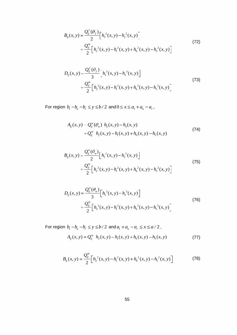
55

2 2

3 2

2 2 2 2

2 1 6 5

( )( , ) ( , ) ( , )

2

( , ) ( , ) ( , ) ( , )2

f

ij f

ij

m

ij

QB x y h x y h x y

Qh x y h x y h x y h x y

(72)

3 3

3 2

3 3 3 3

2 1 6 5

( )( , ) ( , ) ( , )

3

( , ) ( , ) ( , ) ( , )2

f

ij f

ij

m

ij

QD x y h x y h x y

Qh x y h x y h x y h x y

(73)

For region 1 / 2u rb b b y b and

10 u rx a a a ,

5 3

2 1 6 5

( , ) ( ) ( , ) ( , )

( , ) ( , ) ( , ) ( , )

w

ij ij w

m

ij

A x y Q h x y h x y

Q h x y h x y h x y h x y (74)

2 2

5 3

2 2 2 2

2 1 6 5

( )( , ) ( , ) ( , )

2

( , ) ( , ) ( , ) ( , )2

w

ij w

ij

m

ij

QB x y h x y h x y

Qh x y h x y h x y h x y

(75)

3 3

5 3

3 3 3 3

2 1 6 5

( )( , ) ( , ) ( , )

3

( , ) ( , ) ( , ) ( , )2

w

ij w

ij

m

ij

QD x y h x y h x y

Qh x y h x y h x y h x y

(76)

For region 1 / 2u rb b b y b and

1 / 2u ra a a x a ,

2 1 6 5( , ) ( , ) ( , ) ( , ) ( , )m

ij ijA x y Q h x y h x y h x y h x y (77)

2 2 2 2

2 1 6 5( , ) ( , ) ( , ) ( , ) ( , )2

m

ij

ij

QB x y h x y h x y h x y h x y (78)

56

3 3 3 3

2 1 6 5( , ) ( , ) ( , ) ( , ) ( , )2

m

ij

ij

QD x y h x y h x y h x y h x y (79)

4.3.2.2.3. Averaging Schemes for the Stiffness Matrices

In the previous section stiffness matrices are obtained for different regions. In order

to get unique constants for the woven fabric composite, these matrices should be

averaged inside the unit cell. This procedure can be done in different ways; by

averaging stiffness matrices, by averaging compliance matrices or by averaging

both of them. Elastic constants are obtained from averaging extensional stiffness

matrix ( , )ijA x y only.

4.3.2.2.3.1. Series-Parallel Model

In Series-Parallel Model which was used by Naik and Shembekar [10], the elements

along the loading direction are assembled with an iso-stress condition. This

condition is satisfied by averaging the in-plane compliance matrix in the direction of

the applied uniform stress.

Here ( , )ija x y is the in-plane compliance matrix which can be calculated by matrix

inversion of the extensional stiffness matrix, ( , )ijA x y .

1( , ) ( , )ij ija x y A x y (80)

Spatial averaging the compliance matrix in x-direction gives,

0

1( ) ( , )

as

ij ija y a x y dxa

(81)

Then by taking the inverse of the averaged compliance matrix and by spatial

averaging (in y-direction) the stiffness matrix which is obtained from matrix

inversion,

57

1( ) ( )s s

ij ijA y a y (82)

0

1( )

bsp s

ij ijA A y dyb

(83)

By means of these double averaging, averaged stiffness matrix is obtained. Matrix

inversion of the averaged stiffness matrix yields to averaged compliance matrix.

1sp sp

ijija A (84)

Thus, one can find the elastic constants of the WF composite using compliance

matrix through Equations (85) to (88) [21].

11

1x sp

c

Eh a

(85)

22

1y sp

c

Eh a

(86)

12

11

sp

xy sp

a

a (87)

66

1xy sp

Ga

(88)

4.3.2.2.3.2. Parallel-Series Model

Similarly Parallel-Series Model which was used by Naik and Shembekar [10], the

elements normal to the loading direction are assembled with an iso-strain condition.

This condition is satisfied by averaging the coefficients of the in-plane stiffness

matrix in the direction of the applied uniform stress.

Spatial averaging the compliance matrix in y-direction gives,

58

0

1( ) ( , )

bp

ij ijA x A x y dyb

(89)

Then, by taking the inverse of the averaged stiffness matrix and spatial averaging (in

x-direction) the compliance matrix is obtained from matrix inversion,

1( ) ( )p p

ijija x A x (90)

0

1( )

aps p

ij ija a x dxa

(91)

Once the averaged compliance matrix is found, elastic constants of the WF can be

found similarly to the previous model.

11

1x ps

c

Eh a

(92)

22

1y ps

c

Eh a

(93)

12

11

ps

xy ps

a

a (94)

66

1xy ps

Ga

(95)

4.3.2.2.3.3. Series-Series Model

Series-Series Model assumes iso-stress condition in both direction and elastic

constants are obtained on the basis of principle of minimum complementary energy.

Thus it gives the lower bound of the elastic constants. The procedure is based on

double averaging the compliance matrix which is found by matrix inversion of the

stiffness matrix. Once the averaged compliance matrix is found, elastic constants of

the WF composite can be found.

59

1( , ) ( , )ij ija x y A x y (96)

0 0

1( , )

a bss

ij ija a x y dy dxa b

(97)

Therefore,

11

1x ss

c

Eh a

(98)

22

1y ss

c

Eh a

(99)

12

11

ss

xy ss

a

a (100)

66

1xy ss

Ga

(101)

4.3.2.2.3.4. Parallel-Parallel Model

Parallel-Parallel Model assumes iso-strain condition in both direction and elastic

constants are obtained on the basis of principle of minimum potential energy. Thus it

gives the upper bound of the elastic constants. The procedure is based on double

averaging the stiffness matrix. Once the averaged stiffness matrix is found, taking

the matrix inversion of it yields to the averaged compliance matrix. Elastic constants

of the WF composite can be found using averaged compliance matrix.

0 0

1( , )

a bpp

ij ijA A x y dy dxa b

(102)

1pp pp

ijija A (103)

60

Therefore,

11

1x pp

c

Eh a

(104)

22

1y pp

c

Eh a

(105)

12

11

pp

xy pp

a

a (106)

66

1xy pp

Ga

(107)

4.3.2.2.4. Results of the Mini-Level Analysis

In order to calculate the elastic constants of the woven fabric composites, using the

geometric shape functions and averaging schemes presented in the previous

sections, a FORTRAN 77 code was written. By using the shape functions given in

section 4.3.2.2.1, the elastic coefficients are calculated by numerically integrating

the averaged stiffness and compliance coefficients for different averaging schemes

described in the previous section. Trapezoidal numerical integration scheme was

used to perform the numerical integrations, and the step sizes were chosen small

enough to have a little numerical error. The effects of the integration order in series-

parallel and parallel-series are also investigated and it is found that starting the

integrations shown in Equation (81) and Equation (89) in –x direction or –y direction

creates different results. The results form the upper and lower bounds for parallel-

series and series-parallel schemes.

The material property inputs for the developed program are tabulated in Table 10

and the results of the program are tabulated in Table 11 for T300/Epoxy WF

composite. In the structural analysis of the wing, elastic constants calculated by the

upper bounds of parallel-series averaging scheme, which is the recommended

model in the literature [10], has been used. The results of the numerical integrations

for the elastic constants xE , yE , xy , xyG , were used as inputs to the FE program

MSC. Patran directly when creating the 2D orthotropic material.

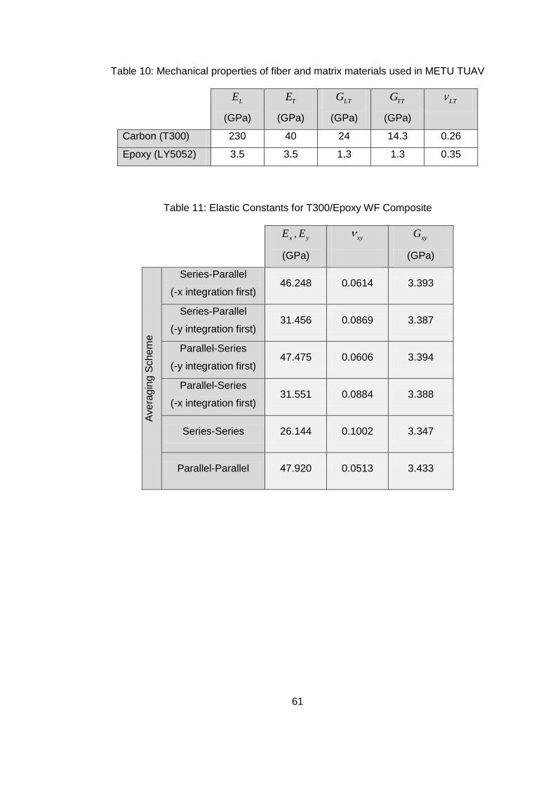
61

Table 10: Mechanical properties of fiber and matrix materials used in METU TUAV

LE

(GPa)

TE

(GPa)

LTG

(GPa)

TTG

(GPa)

LT

Carbon (T300) 230 40 24 14.3 0.26

Epoxy (LY5052) 3.5 3.5 1.3 1.3 0.35

Table 11: Elastic Constants for T300/Epoxy WF Composite

xE , yE

(GPa)

xy

xyG

(GPa)

Ave

rag

ing S

ch

em

e

Series-Parallel

(-x integration first) 46.248 0.0614 3.393

Series-Parallel

(-y integration first) 31.456 0.0869 3.387

Parallel-Series

(-y integration first) 47.475 0.0606 3.394

Parallel-Series

(-x integration first) 31.551 0.0884 3.388

Series-Series 26.144 0.1002 3.347

Parallel-Parallel 47.920 0.0513 3.433

62

CHAPTER 5

STRUCTURAL ANALYSIS OF METU TUAV’S WING WITH FEA

5.1. Introduction

Finite element analysis is a popular numerical method for solving structural

mechanics problems. With the growing computational capabilities of computers,

more complex finite element models can be constructed nowadays. Structural

analysis of METU TUAV‟s wing is done using MSC. MD Nastran 2006 solver.

Preprocessing and post processing of the model is done using MSC. Patran 2006.

The success of the finite element analysis depends on how much the created finite

element model and inputs reflect the real life cases. In Chapter 3, the aerodynamic

loading around the wing was found via CFD which gave accurate force resultants

and distributions. In Chapter 4, the material properties of the woven composites

layers, which are used in manufacturing, are found by a detailed unit cell analysis.

Last but not the least boundary conditions should be chosen very carefully. Although

loading and materials are modeled very good, without proper boundary conditions

the analysis will become inconsistent with the real case. To understand the

response of the structure to boundary conditions, different boundary condition sets

are tried and the most proper one, which is deemed to reflect the real case, is

selected. In structural analysis of the wing, static analysis of the wing is done in two

different loading conditions. These loading conditions are Positive High Angle of

Attack (PHA) and Positive Low Angle of Attack (PLA) conditions which are explained

in Chapter 2 in details. In addition, a dynamic analysis of the composite wing has

also been performed. Firstly a modal analysis has been done to determine the

natural frequencies and the related mode shapes. Secondly a frequency response

analysis of the wing has done to see responses to a varying force at different

locations. Apart from static and dynamic analysis of the wing, finite element model

has been used for determining the torsional stiffness of the wing. Then using this

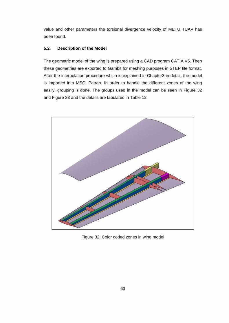
63

value and other parameters the torsional divergence velocity of METU TUAV has

been found.

5.2. Description of the Model

The geometric model of the wing is prepared using a CAD program CATIA V5. Then

these geometries are exported to Gambit for meshing purposes in STEP file format.

After the interpolation procedure which is explained in Chapter3 in detail, the model

is imported into MSC. Patran. In order to handle the different zones of the wing

easily, grouping is done. The groups used in the model can be seen in Figure 32

and Figure 33 and the details are tabulated in Table 12.

Figure 32: Color coded zones in wing model

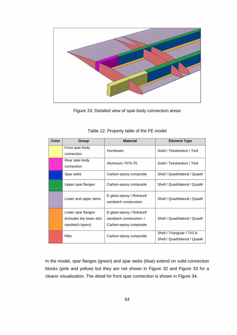
64

Figure 33: Detailed view of spar-body connection areas

Table 12: Property table of the FE model

Color Group Material Element Type

Front spar-body

connection Hornbeam Solid / Tetrahedron / Tet4

Rear spar-body

connection Aluminum 7075-T6 Solid / Tetrahedron / Tet4

Spar webs Carbon-epoxy composite Shell / Quadrilateral / Quad4

Upper spar flanges Carbon-epoxy composite Shell / Quadrilateral / Quad4

Lower and upper skins E-glass-epoxy / Rohacell

sandwich construction Shell / Quadrilateral / Quad4

Lower spar flanges

(includes the lower skin

sandwich layers)

E-glass-epoxy / Rohacell

sandwich construction +

Carbon-epoxy composite

Shell / Quadrilateral / Quad4

Ribs Carbon-epoxy composite Shell / Triangular / Tri3 &

Shell / Quadrilateral / Quad4

In the model, spar flanges (green) and spar webs (blue) extend on solid connection

blocks (pink and yellow) but they are not shown in Figure 32 and Figure 33 for a

clearer visualization. The detail for front spar connection is shown in Figure 34.

65

Figure 34: The detail of front spar connection in FE model

In Figure 33, the front spar extension, which is made of aluminum, goes inside a box

which is fixed to the main bulkhead in the fuselage. On the other hand, the rear spar

end, shown in pink color, is flush with the fuselage, and it is bolted to a rear

bulkhead inside the fuselage through the two holes shown in Figure 33.

The effects of element size to the results are investigated via case study for static

analysis in PLA case. The number of elements, maximum stresses and maximum

tip deflections for fine and course meshes are tabulated in Table 13. As expected,

the maximum deflections for both cases are close to each other but maximum stress

values at elements are very different. Also at elements where intermediate stress

values are seen, the stress values close to each other but to be in the safe side in

terms of material failure fine mesh is used for the structural analyses in FEA.

66

Table 13: Results for different mesh sizes

CASE Number

of shell

elements

Maximum

stress at

shell

elements

(MPa)

Intermediate

stress value

at shell

elements on

upper

flange (MPa)

Number

of solid

elements

Maximum

stress at

solid

elements

(MPa)

Maximum

deflection

(mm)

Fine

mesh 249,268 224 35 1,594,664 104 54.0

Course

mesh 7,941 68 30 3,183 32 54.8

5.3. Boundary Condition Selection

METU TUAV‟s wing is attached to the fuselage bulkheads via cap screws. In rear

spar connection, two M8 helical coils are inserted to the threaded holes of aluminum

section of the rear spar. In the finite element model, translations of nodes inside

these holes are constrained. In principal, helical coils are not inserted up to the end

of holes. Therefore, only those nodes which are in the in the helical coil areas are

constrained. In addition, the nodes on the aluminum part‟s free face which is in

contact with fuselage in –y direction are constrained in this direction because in the

actual mounting, the rear spar is bolted to a bulkhead in the fuselage. During the

installation when the bolts are tightened, the rear spar, shown in pink color in Figure

33, is pulled against the fuselage and the rear spar aluminum becomes constrained

along the wing span direction. However, there always remains a small gap between

the rest of the wing root rib and the fuselage. Therefore, except for the rear spar

end, the rest of the wing root surface is left free.

Front spar is connected to the fuselage by inserting it into a box which is fixed to

fuselage bulkhead. In addition, through two holes, shown in Figure 33, box and the

front spar root are bolted to each other with two fasteners. When the nuts at the

ends of the fasteners are tightened, the box walls are pushed against the spar end

causing almost perfect contact between the box wall and the spar end. Moreover,

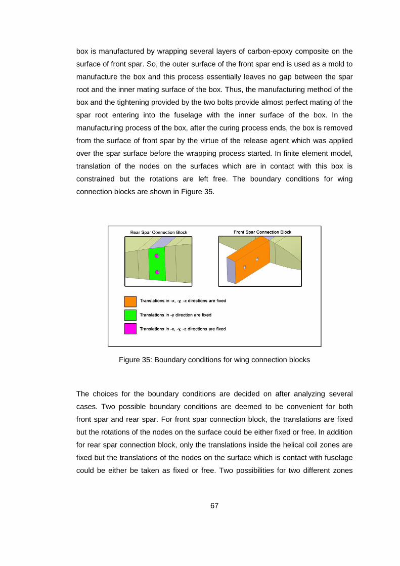
67

box is manufactured by wrapping several layers of carbon-epoxy composite on the

surface of front spar. So, the outer surface of the front spar end is used as a mold to

manufacture the box and this process essentially leaves no gap between the spar

root and the inner mating surface of the box. Thus, the manufacturing method of the

box and the tightening provided by the two bolts provide almost perfect mating of the

spar root entering into the fuselage with the inner surface of the box. In the

manufacturing process of the box, after the curing process ends, the box is removed

from the surface of front spar by the virtue of the release agent which was applied

over the spar surface before the wrapping process started. In finite element model,

translation of the nodes on the surfaces which are in contact with this box is

constrained but the rotations are left free. The boundary conditions for wing

connection blocks are shown in Figure 35.

Figure 35: Boundary conditions for wing connection blocks

The choices for the boundary conditions are decided on after analyzing several

cases. Two possible boundary conditions are deemed to be convenient for both

front spar and rear spar. For front spar connection block, the translations are fixed

but the rotations of the nodes on the surface could be either fixed or free. In addition

for rear spar connection block, only the translations inside the helical coil zones are

fixed but the translations of the nodes on the surface which is contact with fuselage

could be either be taken as fixed or free. Two possibilities for two different zones

68

yield four combinations. These combinations are tabulated in Table 14 and the

results are tabulated in Table 15. The results given in Table 15 were obtained for

PLA load case which was not finalized at the time of calculation so these results

should be taken as for comparison purposes. Some modifications in loading and

material properties are done after proper boundary condition is chosen. By looking

at Table 15, one can see that for Case 1 and Case 3 the maximum stresses for solid

elements are high when compared to the other cases. For Case 1 and Case 3, the

face in contact with the fuselage is freed and the end face of the aluminum block of

the rear spar is fixed only at the helical coil areas. Therefore, high stresses occur

around the helical coil holes. But as it was explained before, when the bolts fixing

rear spar to the fuselage are tightened, the end aluminum block in rear spar, shown

in Figure 33, is pushed against the fuselage and the y displacements along the span

of the wing are constrained. For this reason, fixing the translations of the root end

face of the rear spar in –y direction is deemed to be convenient. On the other hand,

only the displacements on the faces of the front spar root inside the box are fixed

and rotations are left free. This decision was based on the assumption that after

several installations and removals of the wing, there will be slight loosening in the

tightness of the front spar root-fuselage box connection, and therefore it would be

appropriate to let the rotations free. It should also be noted that in the front spar

mating with the fuselage box, there are shell elements representing the carbon

fabrics placed over the hornbeam which is modeled by solid elements. Therefore,

since shell and solid elements use the same node it would also be more appropriate

to let the rotations free because solid elements used in the modeling in this thesis do

not have rotational degree of freedom.

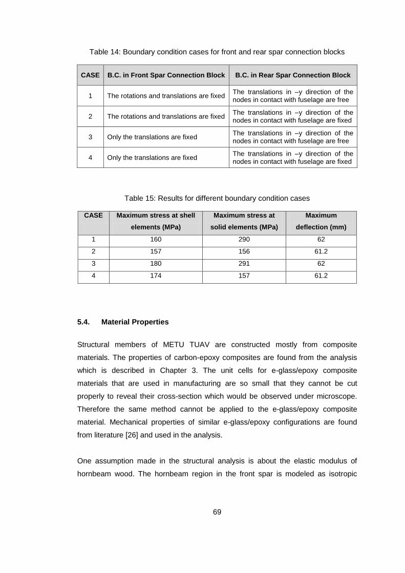
69

Table 14: Boundary condition cases for front and rear spar connection blocks

CASE B.C. in Front Spar Connection Block B.C. in Rear Spar Connection Block

1 The rotations and translations are fixed The translations in –y direction of the nodes in contact with fuselage are free

2 The rotations and translations are fixed The translations in –y direction of the nodes in contact with fuselage are fixed

3 Only the translations are fixed The translations in –y direction of the nodes in contact with fuselage are free

4 Only the translations are fixed The translations in –y direction of the nodes in contact with fuselage are fixed

Table 15: Results for different boundary condition cases

CASE Maximum stress at shell

elements (MPa)

Maximum stress at

solid elements (MPa)

Maximum

deflection (mm)

1 160 290 62

2 157 156 61.2

3 180 291 62

4 174 157 61.2

5.4. Material Properties

Structural members of METU TUAV are constructed mostly from composite

materials. The properties of carbon-epoxy composites are found from the analysis

which is described in Chapter 3. The unit cells for e-glass/epoxy composite

materials that are used in manufacturing are so small that they cannot be cut

properly to reveal their cross-section which would be observed under microscope.

Therefore the same method cannot be applied to the e-glass/epoxy composite

material. Mechanical properties of similar e-glass/epoxy configurations are found

from literature [26] and used in the analysis.

One assumption made in the structural analysis is about the elastic modulus of

hornbeam wood. The hornbeam region in the front spar is modeled as isotropic

70

material although it is not. The hornbeam part which is shown in Figure 12, is

composed of stacks of hornbeam layers whose fiber direction is along the wing

span. In literature [27], elastic modulus of hornbeam parallel to the grain direction is

found and it is used as the elastic constant of hornbeam in MSC. Patran.

Mechanical properties of the materials used in the structural analysis of METU

TUAV are tabulated in Table 16 and Table 17.

Table 16: Mechanical properties of isotropic materials used in METU TUAV

E

(GPa)

US

(MPa)

(tonne/mm3)

Aluminum 7075-T6 70 0.33 524 2.71x10-9

Rohacell 31A [28] 0.026 0.49 - 3.20x10-11

Hornbeam 15.26 0.35 48.3 1.54 x10-9

Table 17: Mechanical properties of 2D orthotropic materials

xE

(GPa)

yE

(GPa)

xyG

(GPa)

xy US

(MPa)

(tonne/mm3)

Carbon/epoxy 47.48 47.48 3.39 0.061 403 1.21x10-9

E-glass/epoxy [26] 26.40 26.40 4.82 0.125 275 1.66 x10-9

71

Table 18: Comparison of results from unit cell analysis and values from literature

xE (GPa) yE (GPa) xyG (GPa) xy

Carbon/epoxy used in METU

TUAV

47.5 47.5 3.4 0.061

T-300 3k/934 plain weave

fabric [26]

62.7 62.0 - -

Celion 3000/E7K8 plain weave

fabric [26]

63.6 65.5 - -

HITEX 33 6k/E7K8 plain weave

fabric [26]

62.8 59.6 - 0.046

AS4 6k/3502 5-harness satin

weave fabric [26]

- - 3.5 -

AS4 6k/PR 500 RTM 5-harness

satin weave fabric [26]

- - 4.4 -

The mechanical properties of carbon/epoxy laminate, which are found via unit cell

analysis in Chapter 4, are compared with similar specimen results available in

literature [26] and it is observed that the results from analyses are close to the

specimen results as shown in Table 18.

5.5. Static Analysis of METU TUAV’s Wing

The first structural analysis of METU TUAV‟s wing is linear static analysis which is

performed using MSC. Nastran‟s linear static solver (NAS101). As described in

Chapter 3, the net forces found from CFD analysis don‟t give desired 3.8g loading

condition which is determined in structural design. The desired 3.8g loading

condition is obtained by multiplying the load case with the necessary factor. Addition

to this correction factor, 1.5 safety factor is applied to the loading condition.

72

Figure 36: The finite element modeling of the tail boom

Moreover, as it is shown in Figure 2, there is also loading from horizontal tail

transferred to the wing via tail boom. For PLA and PHA loading cases loading from

horizontal tail is calculated with simple aerodynamic equations. For simplicity, the

tail boom is modeled with rigid elements (RBE2) available in MSC. Patran‟s library.

Then they are connected to the wing at rear spar and front spar as shown in Figure

36. The calculated horizontal tail load is applied from the tip of the tail boom. The

results are given as contour plots and they are grouped according to the materials.

In composite materials, the result of the layer in which the greatest stress value

occurs, is shown. For each group the margin of safety (MoS) values are calculated

and tabulated.

5.5.1. Results of Static Analysis at Positive Low Angle of Attack Case

Table 19 gives the margin of safety for the front spar. The most critical stress is

seen to occur on the hornbeam at the corner where the spar enters into the box.

Table 19: MoS value for front spar in PLA case

Group Material Margin of Safety (%)

Front Spar Hornbeam 10

73

Figure 37 shows the von Mises stress contours for the front spar core material in

PLA case. It can be seen that maximum stress is below the ultimate tensile strength

of the hornbeam. As Figure 37 shows, the peak stresses occur at the junction where

the front spar enters into the box in the fuselage. The location for the peak stress

was expected because just outside the box the displacements are relaxed on the

outer periphery of the front spar resulting in high displacement gradient which in turn

generates high stresses.

Figure 37: von Mises stress contours for front spar core material in PLA case

Table 20 gives the margin of safety for the rear spar. The most critical stress is seen

to occur on the end aluminum which is used as the core material at the root part of

the rear spar as shown in Figure 33. The critical stress point was at the corner

where the aluminum ends and this is shown in the von Mises stress plot given in

Figure 38. The location of the maximum stress was expected because at that

section there is sudden change in the stiffness in the rear spar. The composite

layers which are wrapped around the aluminum end block extend all the way to the

74

tip forming the box structure of the rear spar of the wing. Thus, there is sudden

change in the core material and this account for a sudden change in the stiffness of

the rear spar resulting in peak stresses.

Table 20: MoS value for rear spar in PLA case

Group Material Margin of Safety (%)

Rear Spar Aluminum 7075-T6 353

Figure 38: von Mises stress contours for rear spar in PLA case

Table 21 and Table 22 present the MoS values for the skin layers for the PLA case.

75

Table 21: MoS values for upper skin layers in PLA case

Group Material Margin of Safety (%)

Upper skin (layer1) E-glass/epoxy 115

Upper skin (layer2) E-glass/epoxy 110

Upper skin (layer3) E-glass/epoxy 131

Upper skin (layer4) E-glass/epoxy 133

Table 22: MoS values for lower skin layers in PLA case

Group Material Margin of Safety (%)

Lower skin (layer1) E-glass/epoxy 18

Lower skin (layer2) E-glass/epoxy 23

Lower skin (layer3) E-glass/epoxy 35

Lower skin (layer4) E-glass/epoxy 41

Figure 39 shows the von Mises stress contours for the skin for the PLA case. The

maximum stresses occur in the nodes at which the RBE2 elements are connected to

the wing. The stresses are also high at the corners at which spar flanges extending

from the wing and root rib intersects. The geometrical discontinuity is the reason for

high stresses at these locations.

76

Figure 39: von Mises stress contours for skin in PLA case

Table 23 presents the margin of safety values for the spar webs and the ribs for the

PLA case. One can see that +x face of front spar and –x face of rear spar have

lower MoS values than the remaining faces by looking at Table 23. The rigid RBE2

elements, which represent the tail boom, are connected to the wing at these

locations. Therefore high stress values were expected at these locations. Figure 40

shows the von Mises stress contours for ribs and spar webs in PLA case. It can be

seen that the first three ribs from root section are more critical than the other outer

ribs.

77

Table 23: MoS values for webs and ribs in PLA case

Group Material Margin of Safety (%)

Front Spar -x face

Web (layer1) Carbon/epoxy 205

Web (layer2) Carbon/epoxy 247

Web (layer3) Carbon/epoxy 241

Web (layer4) Carbon/epoxy 239

Web (layer5) Carbon/epoxy 236

Front Spar +x face

Web (layer1) Carbon/epoxy 25

Web (layer2) Carbon/epoxy 28

Web (layer3) Carbon/epoxy 32

Web (layer4) Carbon/epoxy 36

Web (layer5) Carbon/epoxy 39

Rear Spar -x face

Web (layer1) Carbon/epoxy 10

Web (layer2) Carbon/epoxy 11

Web (layer3) Carbon/epoxy 13

Web (layer4) Carbon/epoxy 14

Web (layer5) Carbon/epoxy 15

Rear Spar +x face

Web (layer1) Carbon/epoxy 360

Web (layer2) Carbon/epoxy 359

Web (layer3) Carbon/epoxy 357

Web (layer4) Carbon/epoxy 355

Web (layer5) Carbon/epoxy 351

Ribs

Ribs (layer1) Carbon/epoxy 182

Ribs (layer2) Carbon/epoxy 233

78

Figure 40: von Mises stress contours for ribs and webs in PLA case

Figure 41 shows the deformation contour for the PLA case. It can be seen that the

tip displacement is 54 mm and this figure is deemed to be a small value owing to the

high stiffness of the wing.

Figure 41: Deformation contour of the whole wing in PLA case

79

5.5.2. Results of Static Analysis at Positive High Angle of Attack Case

Table 24 gives the margin of safety for the front spar. The most critical stress is

seen to occur on the hornbeam at the corner where the spar enters into the box as

in the PLA case.

Table 24: MoS value for front spar in PHA case

Group Material Margin of Safety (%)

Front Spar Hornbeam 43

Figure 42 shows the von Mises stress contours for the front spar core material in

PHA case. It can be seen that maximum stress is below the ultimate tensile strength

of the hornbeam. Similar arguments for the peak stress locations are also valid for

the PHA case as the PLA case.

Figure 42: von Mises stress contour for front spar in PHA case

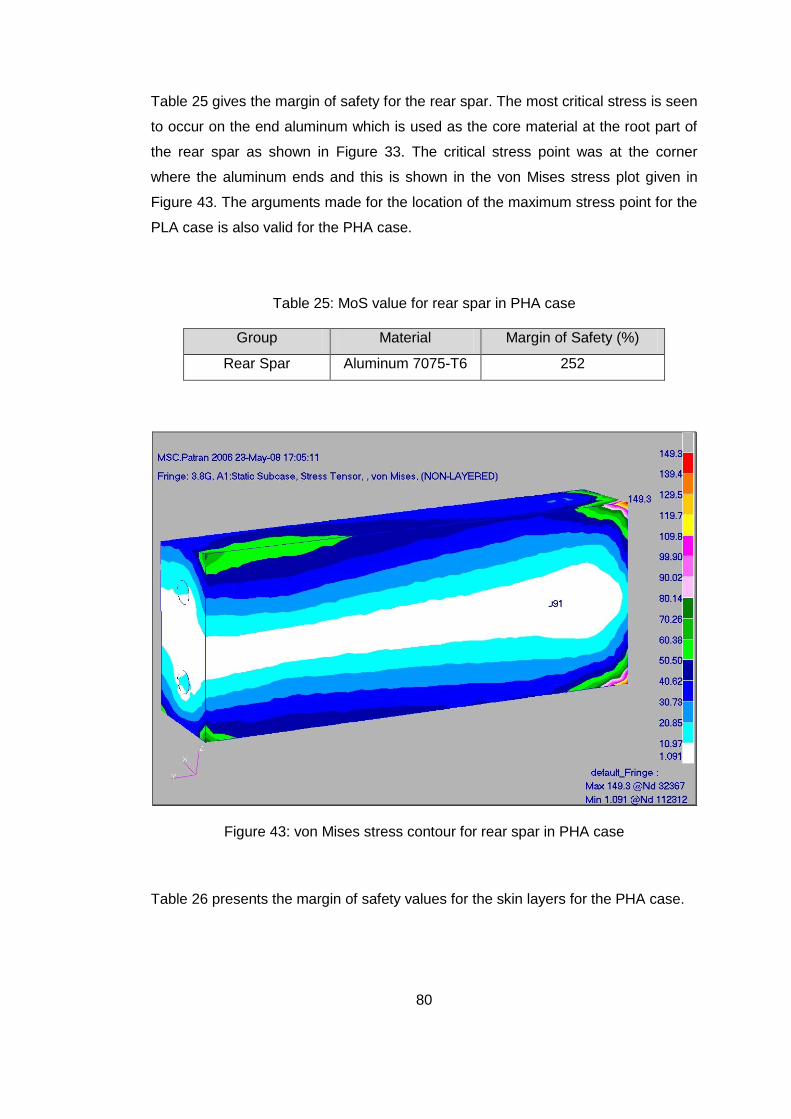
80

Table 25 gives the margin of safety for the rear spar. The most critical stress is seen

to occur on the end aluminum which is used as the core material at the root part of

the rear spar as shown in Figure 33. The critical stress point was at the corner

where the aluminum ends and this is shown in the von Mises stress plot given in

Figure 43. The arguments made for the location of the maximum stress point for the

PLA case is also valid for the PHA case.

Table 25: MoS value for rear spar in PHA case

Group Material Margin of Safety (%)

Rear Spar Aluminum 7075-T6 252

Figure 43: von Mises stress contour for rear spar in PHA case

Table 26 presents the margin of safety values for the skin layers for the PHA case.

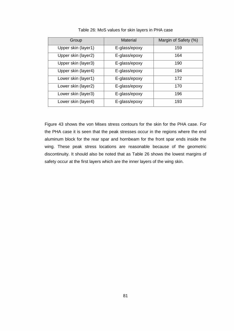
81

Table 26: MoS values for skin layers in PHA case

Group Material Margin of Safety (%)

Upper skin (layer1) E-glass/epoxy 159

Upper skin (layer2) E-glass/epoxy 164

Upper skin (layer3) E-glass/epoxy 190

Upper skin (layer4) E-glass/epoxy 194

Lower skin (layer1) E-glass/epoxy 172

Lower skin (layer2) E-glass/epoxy 170

Lower skin (layer3) E-glass/epoxy 196

Lower skin (layer4) E-glass/epoxy 193

Figure 43 shows the von Mises stress contours for the skin for the PHA case. For

the PHA case it is seen that the peak stresses occur in the regions where the end

aluminum block for the rear spar and hornbeam for the front spar ends inside the

wing. These peak stress locations are reasonable because of the geometric

discontinuity. It should also be noted that as Table 26 shows the lowest margins of

safety occur at the first layers which are the inner layers of the wing skin.

82

Figure 44: von Mises stress contours for skin in PHA case

Table 27 presents the margin of safety values for the spar webs and the ribs for the

PHA case. One can see that the MoS values for PHA are not as low as in PLA case

by looking Table 27. In PLA case, the high stresses occur at tail boom connection

areas whereas in PHA case high stresses occur around areas where the aluminum

and hornbeam blocks start. Tail load is a function of the square of the velocity

therefore it is consistent that tail load for the low velocity PHA case is less than the

one in PLA case. Thus, lower margins of safety for the PLA case is deemed to be

due to higher tail load which would be generated at high velocity.

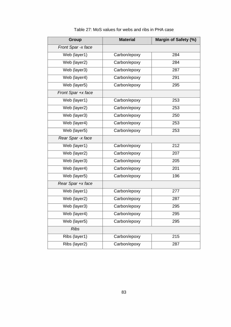
83

Table 27: MoS values for webs and ribs in PHA case

Group Material Margin of Safety (%)

Front Spar -x face

Web (layer1) Carbon/epoxy 284

Web (layer2) Carbon/epoxy 284

Web (layer3) Carbon/epoxy 287

Web (layer4) Carbon/epoxy 291

Web (layer5) Carbon/epoxy 295

Front Spar +x face

Web (layer1) Carbon/epoxy 253

Web (layer2) Carbon/epoxy 253

Web (layer3) Carbon/epoxy 250

Web (layer4) Carbon/epoxy 253

Web (layer5) Carbon/epoxy 253

Rear Spar -x face

Web (layer1) Carbon/epoxy 212

Web (layer2) Carbon/epoxy 207

Web (layer3) Carbon/epoxy 205

Web (layer4) Carbon/epoxy 201

Web (layer5) Carbon/epoxy 196

Rear Spar +x face

Web (layer1) Carbon/epoxy 277

Web (layer2) Carbon/epoxy 287

Web (layer3) Carbon/epoxy 295

Web (layer4) Carbon/epoxy 295

Web (layer5) Carbon/epoxy 295

Ribs

Ribs (layer1) Carbon/epoxy 215

Ribs (layer2) Carbon/epoxy 287

84

Figure 45 shows the Von Misses plot for the rib and spar webs. Figure 45 clearly

shows that the peak stresses occur at the location where the front and rear spar end

blocks ends in the wing. The corners give the peak stresses as expected.

Figure 45: von Mises stress contours for ribs and webs in PHA case

Figure 46: Deformation contour of the whole wing in PHA case

85

Figure 46 shows the deformation contour for the PLA case. It can be seen that the

tip displacement is approximately 58 mm and this figure is deemed to be a small

value owing to the high stiffness of the wing.

To sum up, for both PLA and PHA cases, maximum stress values do not exceed the

strength of the materials in corresponding areas. However, the elements at which

the maximum stresses occur are different for each case. Thus, the importance of

load case study can be understood from these results. The comparison of PLA and

PHA case is tabulated in Table 28.

Table 28: Comparison of peak stress and displacements for PLA and PHA cases

CASE Maximum

Stress (MPa) Material Zone

Maximum

Displacement (mm)

PLA 366 Carbon/epoxy Tail boom-wing

connection 56.2

PHA 149 Aluminum

At the corner

where the

aluminum ends

60.7

5.6. Dynamic Analysis of METU TUAV’s Wing

In order to determine the dynamic characteristics of METU TUAV‟s wing, modal and

frequency response analyses were performed. The results from a normal mode

analysis can be used to guide further possible vibration experiments that may be

conducted on the METU TUAV‟s wing. When planning the vibration testing, best

location for accelerometers can be determined and placing them to nodal points can

be avoided by the help of results from modal analysis. In addition, experimental

vibration results can be compared to the finite element results for mutual verification

of the results. The natural frequencies are also good indicators of the stiffness of the

wing since natural frequencies are directly proportional with stiffness.

86

In modal analysis, MSC. Nastran‟s NAS103 solver is used and natural frequencies

are determined along with the corresponding mode shapes. The results are

tabulated in Table 29 which shows the first three modes and natural frequencies. It

can be seen that the fundamental frequency 16.8 Hz is a high value for the

fundamental frequency of typical wing structures. The low tip deflection for the PLA

and PHA load cases and the high fundamental natural frequency are indication of

high stiffness of the wing.

Table 29: First three normal modes and their frequency

Order Frequency (Hz) Type

1 16.8 First bending

2 71.7 Torsion + Bending

3 84.5 Torsion

The mode shapes of the wing, corresponding to first three natural frequencies, are

shown in Figure 47, Figure 48 and Figure 49, respectively.

Figure 47: Mode shape for the first modal frequency (16.8Hz)

87

Figure 48: Mode shape for the second modal frequency (71.7 Hz)

Figure 49: Mode shape for the third modal frequency (84.5 Hz)

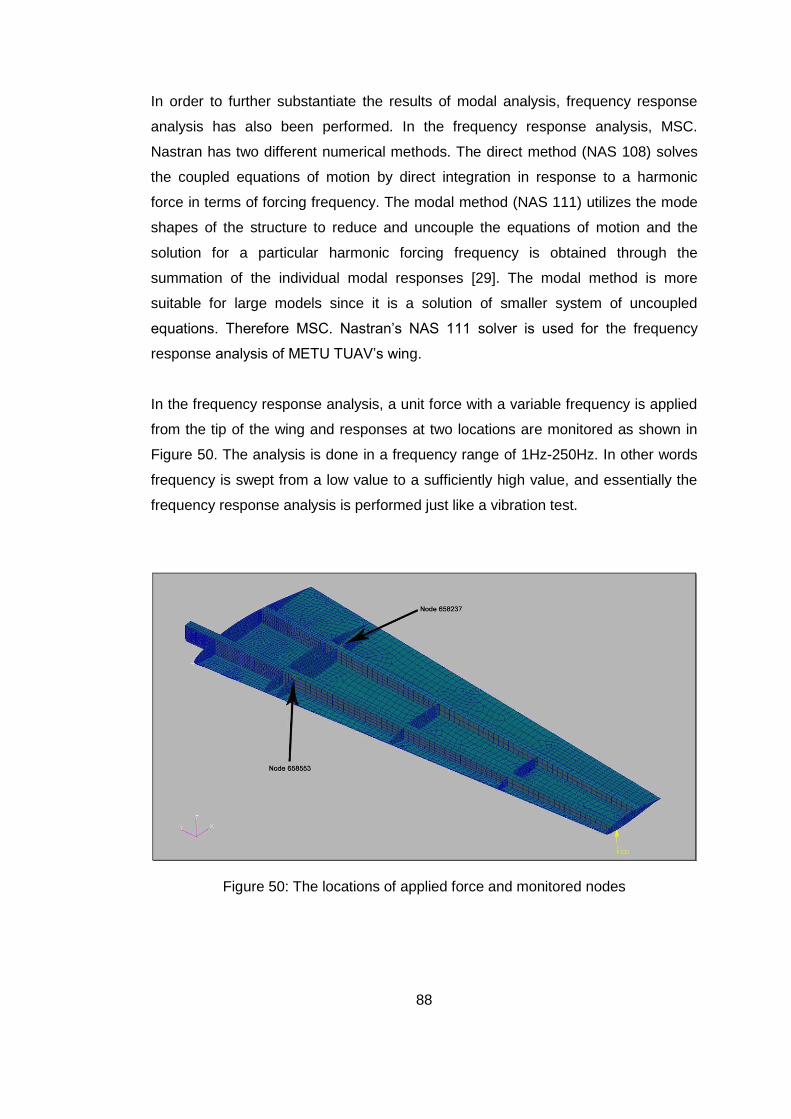
88

In order to further substantiate the results of modal analysis, frequency response

analysis has also been performed. In the frequency response analysis, MSC.

Nastran has two different numerical methods. The direct method (NAS 108) solves

the coupled equations of motion by direct integration in response to a harmonic

force in terms of forcing frequency. The modal method (NAS 111) utilizes the mode

shapes of the structure to reduce and uncouple the equations of motion and the

solution for a particular harmonic forcing frequency is obtained through the

summation of the individual modal responses [29]. The modal method is more

suitable for large models since it is a solution of smaller system of uncoupled

equations. Therefore MSC. Nastran‟s NAS 111 solver is used for the frequency

response analysis of METU TUAV‟s wing.

In the frequency response analysis, a unit force with a variable frequency is applied

from the tip of the wing and responses at two locations are monitored as shown in

Figure 50. The analysis is done in a frequency range of 1Hz-250Hz. In other words

frequency is swept from a low value to a sufficiently high value, and essentially the

frequency response analysis is performed just like a vibration test.

Figure 50: The locations of applied force and monitored nodes

89

The acceleration responses in –z direction at these locations are shown graphically

in Figure 51. As expected, the corresponding frequencies at the peak of response

curves coincide with the natural frequencies found in modal analysis. It is deemed

that the results of the frequency response analysis can be used in evaluating the

results of vibration test which may be conducted on the wing. Especially, in updating

the finite element model the results of the frequency response analysis can be used

together with the results of experimental vibration analysis.

Figure 51: Acceleration response of Node 658237 and Node 658553

5.7. Simplified Torsional Divergence Speed Calculation

Torsional divergence is a static aeroelastic instability which results in catastrophic

failure of a sub-structure of an aircraft such as wing or fin. During flight incremental

90

changes in the aerodynamic pitching moment cause incremental changes in the

twist which induces an incremental angle of attack which in turn causes incremental

change in the pitching moment. Below a certain speed these incremental changes in

the pitching moment and the incremental changes in the angle of attack decrease

until a steady angle of attack value is reached. At low speeds the aerodynamic

moment is resisted by the elastic restoring moment about the elastic axis of the

wing. However, the aerodynamic moment is a function of the square of the flight

velocity whereas the elastic restoring moment is a function of torsional stiffness of

the wing, thus it is independent of the velocity. Therefore, as the flight velocity

increases, a velocity may be reached and at this velocity the elastic restoring

moment can barely resist the aerodynamic moment at the disturbed state. Thus, at

this critical speed wing can disintegrate because it cannot resist the aerodynamic

moment. Beyond the critical speed the incremental changes in the aerodynamic

moment and twist do not decrease but they continuously increase resulting in

catastrophic failure. In this thesis, torsional divergence speed is calculated based on

the slender beam model with the following main assumptions [30]:

Slender straight wing

Elastic axis which is nearly perpendicular to the plane of symmetry of the

airplane

Rigid chordwise segments of the wing; no camber bending

With these basic assumptions the lowest torsional divergence speed for a

rectangular wing with straight elastic axis can be calculated by Equation (108) [30].

2

2D

L

GJU

l ceC (108)

Here:

l is the semi-span of the wing ( 2m )

GJ is the torsional stiffness of the wing at 75% semi-span

c is the mean aerodynamic chord ( 0.54m )

91

e is the distance between aerodynamic center and the elastic axis of

the wing

LC is the lift curve slope of the wing (15.245rad )

is the air density (taken at sea level 31.225 /kg m )

Equation (108) gives the torsional speed for a wing with uniform chord and torsional

stiffness. Early works on aeroelasticity was based on two dimensional

representations of true lifting surfaces. Theodersen used a model of this kind in

analyzing the flutter problem, designating it the „typical section‟ and choosing its

properties to match a cross section 70-75 % of the distance from the root to tip of

the actual wing [31].

Although Equation (108) gives the torsional divergence speed for a rectangular

wing, in this thesis the same formula is used to get an idea of the range of the

torsional divergence speed for the tapered unswept wing. For this purpose, a typical

section is taken at a distance close to 75% of the semi-span measured from the root

of the wing and the properties given in Equation (108) are calculated at this section

except the chord length c. In Equation (108) mean aerodynamic chord, which is

consistent with the derivation of Equation (108), is used.

Mean aerodynamic center at 75% semi-span of METU TUAV‟s wing is found using

document ESDU TD MEMO 6309 from ESDU database which is available at the

Department of Aerospace Engineering of METU.

The structural terms, torsional stiffness GJ and the location of the elastic axis of the

wing can be found using the existing finite element model of the wing.

In order to calculate the GJ at 75% span location, Equation (109), which relates the

sectional torque to rate of twist, is used.

d

T GJdy

(109)

92

One can calculate GJ value at 0.75 semi-span, by applying a known moment, T , at

0.75 semi-span and calculate the rate of twist d

dy value at this position. In order to,

calculate the GJ value, in the finite element model, a 1000 Nmm is applied to a

node which is at the geometric center of the rib which is located very close to 0.75

span position. The rib location is shown in Figure 52 as station B. After a linear static

analysis in MSC. Patran, the deformations of all the nodes at the 75% semi span

section and adjacent sections towards the tip and the root of the can be determined.

Typical sections (E, A, C, D) are shown in Figure 52.

Figure 52: Locations of 75% semi span section and adjacent sections

At a particular section, by using leading edge and trailing edge translations, rotations

( ) at neighbor stations can be determined. The rate of change of the angle of twist

(d

dy) at 0.75 semi-span position can then be found using a high order central

difference formula used for derivative calculations. The central difference formula is

given by Equation (110).

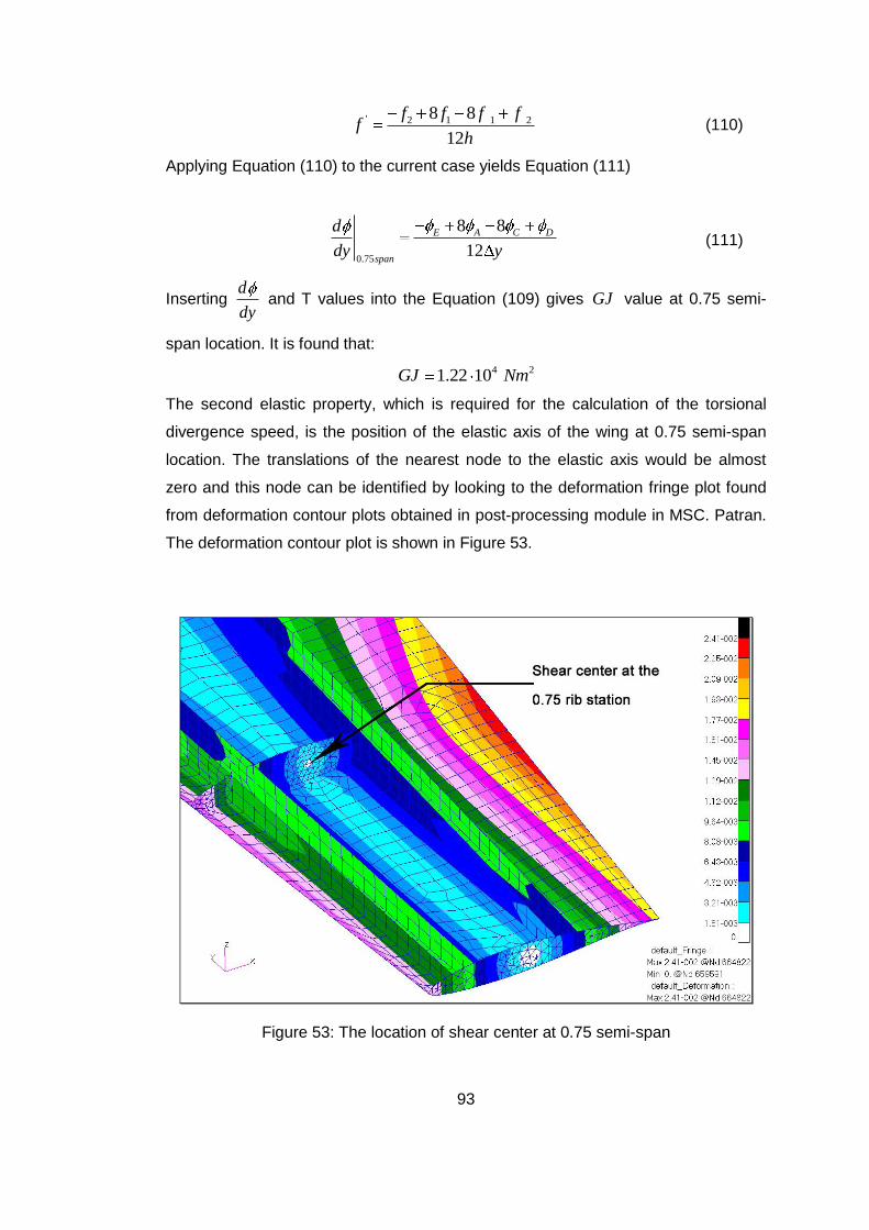
93

' 2 1 1 28 8

12

f f f ff

h (110)

Applying Equation (110) to the current case yields Equation (111)

0.75

8 8

12

E A C D

span

d

dy y (111)

Inserting d

dy and T values into the Equation (109) gives GJ value at 0.75 semi-

span location. It is found that:

4 21.22 10 GJ Nm

The second elastic property, which is required for the calculation of the torsional

divergence speed, is the position of the elastic axis of the wing at 0.75 semi-span

location. The translations of the nearest node to the elastic axis would be almost

zero and this node can be identified by looking to the deformation fringe plot found

from deformation contour plots obtained in post-processing module in MSC. Patran.

The deformation contour plot is shown in Figure 53.

Figure 53: The location of shear center at 0.75 semi-span

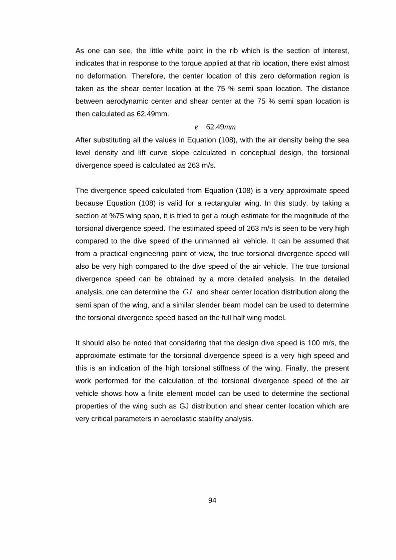
94

As one can see, the little white point in the rib which is the section of interest,

indicates that in response to the torque applied at that rib location, there exist almost

no deformation. Therefore, the center location of this zero deformation region is

taken as the shear center location at the 75 % semi span location. The distance

between aerodynamic center and shear center at the 75 % semi span location is

then calculated as 62.49mm.

62.49e mm

After substituting all the values in Equation (108), with the air density being the sea

level density and lift curve slope calculated in conceptual design, the torsional

divergence speed is calculated as 263 m/s.

The divergence speed calculated from Equation (108) is a very approximate speed

because Equation (108) is valid for a rectangular wing. In this study, by taking a

section at %75 wing span, it is tried to get a rough estimate for the magnitude of the

torsional divergence speed. The estimated speed of 263 m/s is seen to be very high

compared to the dive speed of the unmanned air vehicle. It can be assumed that

from a practical engineering point of view, the true torsional divergence speed will

also be very high compared to the dive speed of the air vehicle. The true torsional

divergence speed can be obtained by a more detailed analysis. In the detailed

analysis, one can determine the GJ and shear center location distribution along the

semi span of the wing, and a similar slender beam model can be used to determine

the torsional divergence speed based on the full half wing model.

It should also be noted that considering that the design dive speed is 100 m/s, the

approximate estimate for the torsional divergence speed is a very high speed and

this is an indication of the high torsional stiffness of the wing. Finally, the present

work performed for the calculation of the torsional divergence speed of the air

vehicle shows how a finite element model can be used to determine the sectional

properties of the wing such as GJ distribution and shear center location which are

very critical parameters in aeroelastic stability analysis.

95

CHAPTER 6

INTEGRAL MANUFACTURING OF A TORQUE BOX

6.1. Introduction

Composite structures are being increasingly used in the primary structures of

aircraft. Because of their poor out-of-plane load transfer capacity, thin walled

composite structures are stiffened by ribs or stringers [32]. In general, in building

semi-monocoque composite structures stiffeners, ribs and skin structures are

integrated to each other by adhesive bonding. Reliability of adhesive bonding is not

predictable although very strong anaerobic structural adhesives are available in the

market and they are frequently used in composite manufacturing. To strengthen the

adhesively bonded regions extra composite layers are applied in fusion areas or

metal doublers are applied by means of riveting. In manufacturing of METU TUAV

and METU mini UAV “Güventürk” adhesive joining technique is used with some

differences. As explained in Chapter 2.3.2, when manufacturing METU TUAV‟s

wing, spars and lower skin are manufactured integrally. But as shown in Figure 14b,

the upper skin is adhesively joined to the upper surfaces of spars and ribs. This

adhesive bonding technique introduces extra weight to structure. In METU TUAV,

this is approximately 15% of the total weight of the wing. If a fully integrated and

continuous upper skin-spar-rib-lower skin structure was manufactured, this extra

weight could have been prevented. The composite skin-stiffener integrity problem is

generally handled by making upper and lower parts integrally by themselves and

then joining them with a different technique. The costs and complexity of these

techniques stand in a wide range. In NASA‟s “AST Composite Wing Program” [33],

the integrity between skin and stiffeners are achieved by stitching process which is

basically involves sewing high tensile thread through stacked ply layers to produce a

preform with a 3D structure [12] as shown in Figure 54. Then the preform is resin

infused by the help of vacuum bagging in an autoclave. When the investment costs

96

of autoclave and stitching machine are considered it can be seen that this procedure

is not suitable for low cost small aircrafts or UAVs.

(a) (b) (c)

Figure 54: Stitching of (a) stringer to skin, (b) rib to skin, (c) skin with integral spar caps [33]

Another example of integrated manufacturing of skin-stiffener assembly is

demonstrated by Lockheed Martin Space Systems (LMSS), to minimize the

fabrication cost of one of the largest and most complex components of Trident II D5

missile system by using vacuum-assisted resin transfer molding (VARTM). Labor,

time and overall cost were reduced with cost savings as high as 75% and 61-part

assembly was manufactured at once therefore 376 fasteners were eliminated [34].

VARTM is also used to manufacture a fully integral skin-stringer assembly by

Mahfuz et al [32]. The end product of their work is shown in Figure 55.

97

Figure 55: Integral composite skin-stringer assembly [32]

In this thesis similar manufacturing steps of Mahfuz et al [32] are followed to

manufacture a composite box structure with some differences. At the end a fully

skin-stringer integrated composite box structure which is manufactured using

VARTM, is demonstrated.

6.2. Vacuum-Assisted Resin Transfer Molding (VARTM)

The VARTM process is a composite fabrication process by which a dry fiber preform

is vacuum-bagged against a single-sided tool and is infused with resin that is drawn

in a controlled manner into the evacuated preform [26]. The schematic of the

VARTM process is shown in Figure 56 and photographs of a VARTM setup for

manufacturing of a composite plate are shown in Figure 57 and in Figure 58. The

resin is introduced to the system through ports or flow lines. The distribution medium

covering the workpiece makes the resin easy to infiltrate to the preform and

eliminates the dry spots. The peel ply on the preform is for easy removal of the

distribution medium and vacuum bag from the workpiece. Spiral tubes are tubes that

are cut in a spiral shape. Spiral tubes are generally placed all around laminate as

shown in Figure 57, and they suck the air under the vacuum bag until the resin flows

and wet all the laminate which is to be manufactured. Through the fittings at the end

of these tubes, they are connected to the resin catch tank. The shape of the tubes

allows the excess resin in the system to be sucked and transferred to the resin catch

tank. Resin catch tank is connected to the vacuum pump which keeps it under

vacuum all the time.

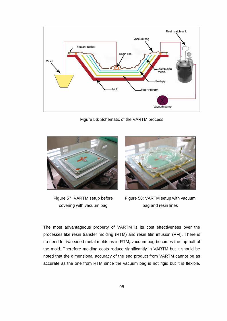
98

Figure 56: Schematic of the VARTM process

Figure 57: VARTM setup before

covering with vacuum bag

Figure 58: VARTM setup with vacuum

bag and resin lines

The most advantageous property of VARTM is its cost effectiveness over the

processes like resin transfer molding (RTM) and resin film infusion (RFI). There is

no need for two sided metal molds as in RTM, vacuum bag becomes the top half of

the mold. Therefore molding costs reduce significantly in VARTM but it should be

noted that the dimensional accuracy of the end product from VARTM cannot be as

accurate as the one from RTM since the vacuum bag is not rigid but it is flexible.

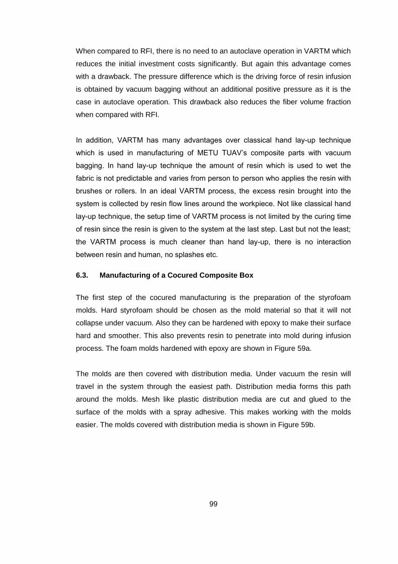
99

When compared to RFI, there is no need to an autoclave operation in VARTM which

reduces the initial investment costs significantly. But again this advantage comes

with a drawback. The pressure difference which is the driving force of resin infusion

is obtained by vacuum bagging without an additional positive pressure as it is the

case in autoclave operation. This drawback also reduces the fiber volume fraction

when compared with RFI.

In addition, VARTM has many advantages over classical hand lay-up technique

which is used in manufacturing of METU TUAV’s composite parts with vacuum

bagging. In hand lay-up technique the amount of resin which is used to wet the

fabric is not predictable and varies from person to person who applies the resin with

brushes or rollers. In an ideal VARTM process, the excess resin brought into the

system is collected by resin flow lines around the workpiece. Not like classical hand

lay-up technique, the setup time of VARTM process is not limited by the curing time

of resin since the resin is given to the system at the last step. Last but not the least;

the VARTM process is much cleaner than hand lay-up, there is no interaction

between resin and human, no splashes etc.

6.3. Manufacturing of a Cocured Composite Box

The first step of the cocured manufacturing is the preparation of the styrofoam

molds. Hard styrofoam should be chosen as the mold material so that it will not

collapse under vacuum. Also they can be hardened with epoxy to make their surface

hard and smoother. This also prevents resin to penetrate into mold during infusion

process. The foam molds hardened with epoxy are shown in Figure 59a.

The molds are then covered with distribution media. Under vacuum the resin will

travel in the system through the easiest path. Distribution media forms this path

around the molds. Mesh like plastic distribution media are cut and glued to the

surface of the molds with a spray adhesive. This makes working with the molds

easier. The molds covered with distribution media is shown in Figure 59b.

100

Over the distribution mesh peel ply is wrapped as the next step. Peel ply is a

permeable cloth which is in contact with the preform and eases the removal of

workpiece. Peel ply covered molds are shown in Figure 59c

Around the peel ply e-glass woven fabrics are rolled over tightly. During the rolling

over the woven fabric “tac-strip” pieces are applied between the layers. Tac-strip is a

fiberglass fabric mesh tape coated on both sides with a pressure sensitive adhesive.

It stays inside the layers and become a member of the fabric stacks without

hampering the structural properties. Fiberglass sticky tape holds the preform in one

piece and avoids the movement of the preform around the mold. Woven fabric

preforms around the molds are shown in Figure 59d.

A glass surface, which is used as the tool plate, is coated with a release agent. This

surface will be the mold surface for the lower surface of the workpiece. A double

sided adhesive tape is applied to the glass surface in order to hold the spiral tube

through which trapped air under the vacuum bag and excess resin in the system will

be sucked. A layer of distribution media is laid on the glass surface, or the tool plate,

which will ease the wetting of the lower surface of the preform. The distribution

media is covered with peel ply as it was done in molds. These steps are shown in

Figure 59e and Figure 59f. In Figure 59e spiral tube is placed on top of a double

sided tape in order not to move during the vacuuming operation. The air will be

sucked from the two ends of the spiral tube through the end plastic L shaped joints.

On to the peel ply two layer of e-glass are laid and three preforms around molds are

put together on top of these layers. Finally two more layers which will form the top

surface of the workpiece are laid on these molds as shown in Figure 59g. Over the

preform is a peel ply layer is put to ease the removal of the workpiece after the

curing. As a final layer distribution mesh is laid on top of the peel ply.

It should be noted that there is always a peel ply layer between the preform and the

distribution mesh.

In front of the preform a resin flow line is placed and similarly another resin flow line

is placed on top of the preform. As it is shown in Figure 59h, the resin is brought into

101

the system through the plastic hoses and these hoses are pushed into the resin flow

lines through the opening in the middle of the resin flow line which is made of some

sort of rubber. Once the resin enters into the resin flow line by the help of the

suction, which will be applied through the spiral tube, the edges of the resin flow line

helps the resin to travel along the edge of the resin flow line so resin starts to infuse

into the front edge of the preform homogenously.

Rubber sealant tape is applied around the workpiece and tubes are plugged into the

flow lines and spiral tube as shown in Figure 59i and Figure 59j. Rubber sealant will

be used to secure the vacuum bag and seal whatever remains inside the bag from

the external environment. In Figure 59i the plastic hose inside the spiral tube is

seen. The plastic hose is pushed into the spiral tube from the both ends and its

periphery is sealed against the rubber sealant tape by the again using the same

rubber sealant tape. In a similar fashion the plastic tubes are placed inside the resin

flow lines, and sealed against the peripheral rubber sealant tape which is placed all

around the workpiece and this is shown clearly in Figure 59j. The plastic hoses

shown in Figure 59j will be inserted into the resin bucket to bring in resin into the

system once the vacuum is applied and air inside the bag is sucked away from the

spiral tube and its end hoses. However, before the application of the vacuum, the

plastic tubes which will carry the resin are squeezed by the clamps as shown in

Figure 59l.

As it is shown in Figure 59k the whole setup is then covered with vacuum bag and

vacuum is applied to the system Figure 59m shows the system after the vacuum is

applied. The applied vacuum in the bag compacts the preform and this is a perfect

moment to seal check before the resin is introduced to the system. It should be

again noted that as shown in Figure 59l, the end of two plastic tubes which are

connected to the flow lines, are clamped at this moment so resin does not enter into

the system. Therefore, any air escape can be monitored and leakage test can be

conducted.

Then, the two clamped plastic tubes connected to the flow lines are immersed to the

resin case and clamps are released. This way resin enters into the preform from the

one end and due to the suction from the other end, the resin start to travel along the

102

workpiece. At this point, it should be noted that since the suction is applied from the

lower surface, the resin which enters into the preform from the lower resin flow line

will travel faster compared to the resin which enters into the perform from the upper

resin flow line. This is because the resin distributed from the top resin flow line will

be forced to travel around the three molds which are wrapped with composite fabric.

Therefore, in order to match the arrival times of the resin entering into the preform

from the bottom and top resin flow lines, the clamp of the top resin flow line is

released earlier; the location of the resin front is observed. Then, the bottom clamp

is released accordingly. The wetted preform is shown in Figure 59n and Figure 59o.

Figure 59n and Figure 59o show that the whole workpiece is clamped along the

sides to increase the compaction pressure during the curing process.

After curing process, the vacuum bag and peel ply and distribution mesh around the

outer surface of the workpiece are all removed from the cured workpiece and

workpiece is removed from the glass surface. At this point the foam molds are still a

part of the workpiece. The workpiece before the removal of molds is shown in Figure

59p.

The last step is the removing the foam molds, peel ply and distribution media inside

the composite box structure. It should be reminded that the foam molds were initially

wrapped with peel ply and the distribution media for easy removal of the workpiece

and for better resin distribution. The foam molds are removed using a synthetic

thinner which basically melts the foam chemically. The remaining peel ply with the

distribution mesh on it is then removed by the help of a chisel. The peel ply eases

the removal operation very much and it does not let the distribution media to stick to

the workpiece. The cleaned final product is shown in Figure 59q and Figure 59r.

As Figure 59q and Figure 59r show, with this operation it is possible to produce

multi-cell box beam structures in one operation. This way the vertical webs and the

horizontal upper and lower skins are integrally manufactured by the co-curing action.

It is deemed that this method can also be applied to the production of sub-structures

such as wings, control surfaces and horizontal and vertical tails in aerospace

applications.

103

(a) (b)

(c) (d)

(e) (f)

Figure 59: Manufacturing steps of a cocured composite box

104

(g) (h)

(i) (j)

(k) (l)

Figure 59: Manufacturing steps of a cocured composite box (continued)

105

(m) (n)

(o) (p)

(q) (r)

Figure 59: Manufacturing steps of a cocured composite box (continued)

106

CHAPTER 7

CONCLUSION

In this study structural design, analysis and composite manufacturing applications

for a tactical UAV is introduced. Since wing is the most critical part of an aircraft, the

study is focused on the composite wing of METU TUAV.

Firstly, the design features of METU TUAV are explained. In structural design, the

structural requirements are determined from UAV Systems Airworthiness

Requirements (USAR) [5] which is prepared by USAR Working Group. Structural

design of the wing is introduced together with the composite manufacturing of the

wing. V-n diagram for the tactical UAV is established based on the limit loads

specified in USAR and the design critical loads are decided to be calculated at the

minimum maneuvering speed VA and dive speed VD. The manufacturing steps of

the composite wing is introduced with sufficient detail to help the reader in following

the analysis procedure which requires understanding of the internal structural layout

and certain manufacturing details of the composite wing.

After determining the loading scenarios in structural design, aerodynamic loading

around the wing is found via CFD analysis. The results are compared with the

analytical studies which were done during conceptual design phase of METU TUAV.

In order to show the effect of the computational mesh, a case study is also

performed for CFD analysis and it is shown that a more fine CFD mesh is not

needed for analysis. At the end of the CFD analysis, the nodal forces on the wing

surface mesh are transferred to FEA mesh via interpolation.

The composite fabrics, which are used in manufacturing of METU TUAV, are in plain

woven fabric form. Therefore, classical laminate theory cannot be applied directly to

the composite materials that include woven fabrics. In order to find the mechanical

107

properties of plain woven composite materials used in the manufacturing, a detailed

unit cell analysis is performed. A FORTRAN code is written to calculate the effective

elastic properties of the plain weave composite fabric. The code calculates the

effective elastic properties on the geometrical unit cell domain which repeats itself in

the fabric. Unit cell is defined by certain shape functions which are typically used in

the literature and trapezoidal numerical integration scheme was used to numerically

get the effective elastic constants of the woven fabric.

After the aerodynamic load calculation and material characterization steps, the

structural analysis of the METU TUAV‟s wing is performed. Linear static analysis of

the wing is performed at two different loading conditions which are positive high

angle of attack and positive low angle of attack. Results of static analyses are

shown in details with contour plots and tables showing the margins of safety of

different elements of the composite wing. Modal and frequency response analyses

of the wing were also performed to investigate the dynamic properties of the wing.

Finally, torsional divergence speed of METU TUAV is found by a simplified method

based on slender beam model. Structural properties are extracted from the finite

element model and aerodynamic properties such as the location of aerodynamic

center are determined by using a software of ESDU database.

Based on the structural analyses results, it is concluded that the wing is safe based

on static limit load analyses performed at minimum maneuvering and dive speeds.

Deflection and dynamic analysis showed that the wing was relatively stiff, and this

effect was also reflected in the approximate divergence speed which turned out to

be quite high. Thus, before the first flight, sufficient level of confidence has been

built up in the structural integrity of the wing structure.

In addition, co-cured composite manufacturing of structural members is explained in

the last chapter. The merits of manufacturing multi-cell closed box beams with co-

cured stiffener/spar and skin assembly is discussed. To manufacture a co-cured

composite multi-cell box structure, a procedure is explained which uses vacuum

assisted resin transfer molding (VARTM) technique. With the help of this procedure,

a composite multi-cell box which is manufactured successfully in Aerospace

Engineering Department of METU and the manufacturing steps are described in

108

detail with relevant pictures taken at the intermediate steps during the

manufacturing.

The following studies are proposed as future work:

CFD analysis of the wing can be improved by using a Navier-Stokes solver.

Also half body and tail can be introduced to the new model; therefore fluid

interactions around the whole aircraft can be investigated.

Gust load analysis can be performed using the related airworthiness

standards. This way time dependent stress analysis can be carried out.

The co-cured composite manufacturing technique can be applied to an

actual structural part of METU TUAV, such as vertical or horizontal tail, and

these structures can be manufactured in one piece eliminating the need for

secondary bonding

A detailed static and dynamic aeroelastic analysis can be performed based

on the existing finite element model.

Mechanical properties of woven fabric composite can be found using finite

element techniques and compared with the existing results found from unit

cell analysis. Also mechanical tests can be performed to verify these results.

Failure analyses of the composite wing structure can be performed. Initial

failure and progressive failure analyses can be performed in order to

substantiate the residual strength of the wing.

109

REFERENCES

1. Federation of American Scientists web site,

“http://www.fas.org/irp/program/collect/uav.htm”, as accurate of 28 April,

2008

2. Unmanned Vehicle Systems International web site, “http://www.uvs-

info.com/Yearbook2007/158_UAS_Categories-Tables-Figures.pdf”, as

accurate of 28 April, 2008

3. Raymer, Daniel P., “Aircraft Design: A Conceptual Approach”, AIAA

Education Series, 1992.

4. Niu, M. C. Y., “Airframe Structural Design”, Conmilit Press LTD., 1988

5. USAR Working Group 2005. UAV Systems Airworthiness Requirements

(USAR) Version 3.

6. Anderson, J.D., “Aircraft Performance and Design”, McGraw-Hill, 1999

7. Turgut, T., “Manufacturing and Structural Analysis of a Lightweight Sandwich

Composite UAV Wing”, 2007

8. Abbot, I. H. and Von Doenhoff, A. E., “Theory of Wing Sections”, Dover

Publications Inc., 1959, pp.522.

9. Netcomposites web site,

“http://www.netcomposites.com/education.asp?sequence=43”, as accurate

of 28 April, 2008.

10. Naik, N. K. and Shembekar, P. S., “Elastic Behavior of Woven Fabric

Composites: I-Lamina Analysis”, Journal of Composite Materials, Vol. 26,

No. 15, 1992, pp. 2196-2225.

11. Shang Zhong Sheng and Suong Van Hoa., “Three Dimensional Micro-

Mechanical Modeling of Woven Fabric Composites”, Journal of Composite

Materials, Vol. 35, No.19, 2001, pp. 1701-1729

12. L. Tong, A.P. Mouritz and M.K. Bannister, “3D Fibre Reinforced Polymer

Composites”, Elsevier, 2002, pp. 70.

110

13. Levent Onal and Sabit Adanur., “Modeling of Elastic, Thermal, and

Strength/Failure Analysis of Two-Dimensional Woven Composites-A

Review”, Applied Mechanics Reviews, Vol. 60, January 2007, pp. 37-49

14. National Wiper web site,

“http://www.nationalwiper.com/tools_and_links/glossary/default.html”, as

accurate of 28 April, 2008.

15. The A to Z of Materials web site,

“http://www.azom.com/details.asp?ArticleID=1091#_Plain_Weave”, as

accurate of 28 April, 2008.

16. Halpin, J.C., Jerine, K. and Whitney, J.M., “The Laminate Analogy for 2- and

3-Dimensional Composites”, Journal of Composite Materials, 5:36-49, 1971

17. Ishikawa, T. and T.-W. Chou. 1983. “One Dimensional Micromechanical

Analysis of Woven Fabric Composites,” AIAA Journal, 21(12):1714-1721.

18. Ishikawa, T. and T.-W. Chou. 1982. “Stiffness and Strength Behavior of

Woven Fabric Composites,” Journal of Materials Science, 17:3211-3220

19. Ishikawa, T. 1981. “Anti-Symmetric Elastic Properties of Composite Plates of

Satin Weave Cloth,” Fibre Science and Technology, 15:127-145.

20. Tsu-Wei Chou, “Micro-structural Design of Fiber Composites”, Cambridge

University Press, 2005, pp. 302.

21. Falzon, P.J., Herzberg, I., and Karbhari, V.M., 1996, “Effects of Compaction

on the Stiffness and Strength of Plain Weave Fabric RTM Composites,”

Journal of Composites Materials, 30, pp. 1210-1247

22. B.N. Cox and M.S. Dadkhah, "The Macroscopic Elasticity of 3D Woven

Composites," J. Comp. Mater., 29, 795-819 (1995).

23. Hashin, Z., “Theory of Fibre Reinforced Materials,” CR-1974, NASA, 1972.

24. Hashin, Z., “Analysis of Composite Materials-A Survey,” J. Appl. Mech.,

50:481, 1983.

25. Lekhnitskii, S. G., “Theory of Elasticity of an Anisotropic Body”, Moscow: MIR

Publishers, 1981.

26. Department of Defense Handbook, “Composite Materials Handbook, Volume

2: Polymer Matrix Composites Material Properties”

27. Aydın, S., Yardımcı, M.Y., Ramyar, K., “Mechanical Properties of Four

Timber Species Commonly Used in Turkey,” Turkish J. Eng. Env. Sci. 31:19-

27, 2007.

111

28. Aerospatiale Aeronautique, Composite Stress Manual, Z10-1/3

29. MSC. Nastran - Basic Dynamics Analysis User‟s Guide, MSC.Software

Corporation

30. Bisplinghoff, R.L., Asley, H. and Halfman, R.L., “Aeroelasticity”, Dover

Publications, pp. 421-434, 1996.

31. Theodorsen, T, “General Theory of Aerodynamic Instability and the

Mechanism of Flutter”, NACA Report 496, 1935.

32. Mahfuz, H., Majumdar, P., Saha, M., Shamery, F. and Jeelani, S., “Integral

Manufacturing of Composite Skin-Stringer Assembly and Their Stability

Analysis,” Applied Composite Materials 11: 155-171, 2004.

33. Karal, M., “AST Composite Wing Program – An Executive Summary,” CR-

2001-210650-NASA, 2001.

34. Tatum, S., “VARTM Cuts Costs”, Reinforced Plastics 45(5), May 2001, 22.

112

APPENDIX A

INTERPOLATION OF CFD DATA INTO FINITE ELEMENT MODEL

Creating the Geometry

Geometry of the wing can be created using any CAD program from which the

geometry can be exported in general file formats, such as STEP (Standard

for the Exchange of Product), IGES (Initial Graphics Exchange

Specification). In this study, CATIA V5 is used as CAD program. The edges

and zones on which different mesh properties wanted can be defined in the

CAD program therefore manipulation with the geometry in the next step

(preprocessing the CFD mesh) can be skipped.

Figure 60: CAD model of the wing

It is observed that in most programs exporting the geometry in STEP file

format gives better results than the other ones.

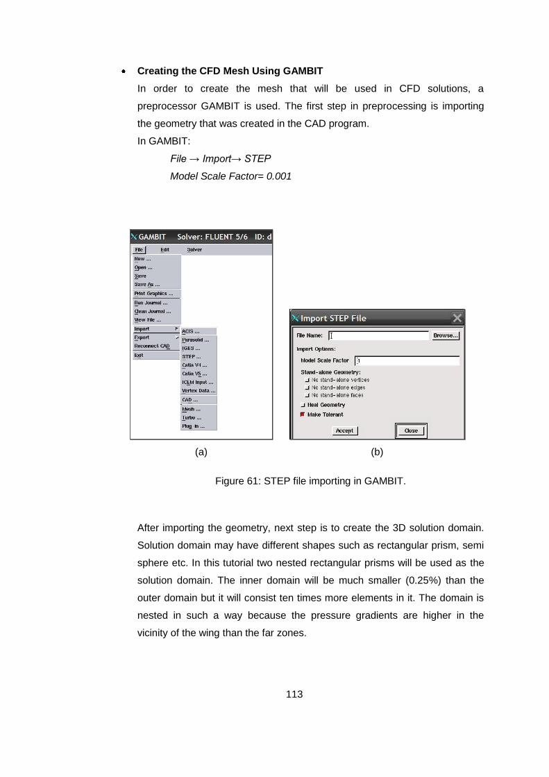
113

Creating the CFD Mesh Using GAMBIT

In order to create the mesh that will be used in CFD solutions, a

preprocessor GAMBIT is used. The first step in preprocessing is importing

the geometry that was created in the CAD program.

In GAMBIT:

File → Import→ STEP

Model Scale Factor= 0.001

(a) (b)

Figure 61: STEP file importing in GAMBIT.

After importing the geometry, next step is to create the 3D solution domain.

Solution domain may have different shapes such as rectangular prism, semi

sphere etc. In this tutorial two nested rectangular prisms will be used as the

solution domain. The inner domain will be much smaller (0.25%) than the

outer domain but it will consist ten times more elements in it. The domain is

nested in such a way because the pressure gradients are higher in the

vicinity of the wing than the far zones.

114

In GAMBIT:

Create the inner domain

Geometry→ Volume→ Create Real Brick

Width(X) = 3

Depth(Y) = 4

Height (Z) = 2

Move the inner domain to its appropriate position

Geometry→ Volume→ Move/Copy

Global x = 0.5

Global y = -2

Global z = 0

Create the outer domain

Geometry→ Volume→ Create Real Brick

Width(X) = 40

Depth(Y) = 15

Height (Z) = 16

Move the outer domain to its appropriate position

Geometry→ Volume→ Move/Copy

Global x = 9

Global y = -7.5

Global z = 0

Subtract the volumes from each other

Geometry→ Volume→ Subtract

Volume = volume3 (outer domain)

Subtract volume = volume2 (inner domain) while retaining the

volume2

Geometry→ Volume→ Subtract

Volume = volume2 (inner domain)

Subtract volume = volume1 (imported wing geometry)

115

Clean the duplicate surfaces

Tools→ Geometry Cleanup→ Clean Up Duplicate Surfaces

Tolerance = Default

Update→ Auto

Creating edge meshes of the surface mesh on the wing is the next step.

Note that, the following procedures may differ from geometry to geometry.

Also computing power will determine how fine or course the mesh will be.

Mesh→ Edge→ Edges (select the edges of the wing)

Interval Size = 0.01

Mesh→ Face→ Faces (select the faces of the wing)

Elements = Tri

Type = Pave

Next step is creating the size functions and creating the volume mesh. The

size functions will determine the growth rate of the volume mesh starting

from the surface mesh. In the inner domain the growth will be smaller than

the outer one since a finer mesh is wanted in the inner domain.

Tools→ Size Function→ Create Size Function

Type = Meshed

Faces = Wing Surface Faces

Volume = volume2 (inner domain)

Growth rate = 1.09

Mesh→ Volume→ Volumes (select the inner domain)

Elements = Tet/Hybrid

Type = TGrid

116

Figure 62: Inner CFD domain

Tools→ Size Function→ Create Size Function

Type = Meshed

Faces = Surfaces of the inner domain (5 surfaces)

Volume = volume3 (outer domain)

Growth rate = 1.2

Mesh→ Volume→ Volumes (select the outer domain)

Elements = Tet/Hybrid

Type = TGrid

Figure 63: The whole CFD domain

117

The last step of the mesh generation will be defining the zones and boundary

conditions.

Zones→ Specify Boundary Types

Select the wing surfaces and assign them WALL boundary condition

Select the interfaces of inner domain and outer domain (5 surfaces)

and assign them INTERIOR

Assign other boundary conditions as shown in the figure below.

Figure 64: Boundary conditions for CFD analysis

Zones→ Specify Continuum Types

Type = Fluid

Volumes = Select the inner and outer domains

Finally the resulting mesh can be exported.

File → Export→ Mesh

Running the FLUENT Analysis

Fluent → Run→ 3D

File → Read→ Case→ *.msh

118

Grid → Check

Grid→ Reorder→ Domain

Define→ Model→ Solver

Figure 65: Selecting the solver properties in Fluent.

Define→ Model→ Viscous→ Inviscid

Define→ Boundary Conditions→ Zone=Inlet→ Type=Velocity Inlet

Figure 66: Velocity inlet boundary condition

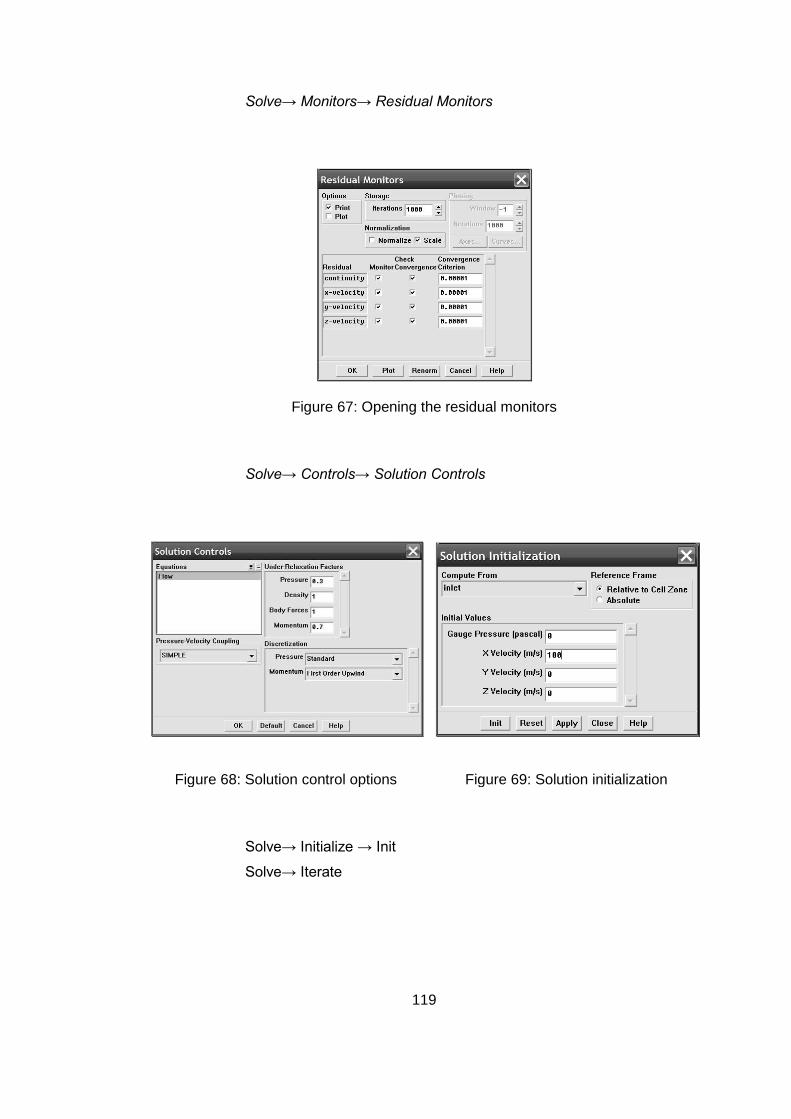
119

Solve→ Monitors→ Residual Monitors

Figure 67: Opening the residual monitors

Solve→ Controls→ Solution Controls

Figure 68: Solution control options Figure 69: Solution initialization

Solve→ Initialize → Init

Solve→ Iterate

120

Figure 70: Starting the iteration process in Fluent

The iteration can be stopped after the residuals converged in first order

upwind solution and the solution scheme can be changed to second order

upwind solution for better accuracy. After the iterations are stopped, the

nodal forces and corresponding surface meshes can be exported to Nastran.

Exporting the Nodal Forces

So far, the CFD solution procedure in Gambit and Fluent is explained. In

order to perform interpolation procedure a new volume mesh should be

created. The surface meshes on wing surfaces should be created regarding

the new FEM mesh that will be exported to FE program. The mesh intensity

and properties should be chosen carefully keeping in mind the FE analysis.

After creating new volume mesh from this surface mesh, it should be

imported into Fluent. As explained in Chapter 3, the geometrical domains of

the CFD solution mesh and new interpolation mesh should be identical.

First step is writing the interpolation data from CFD solution.

File → Interpolate→ Write Data→ Write

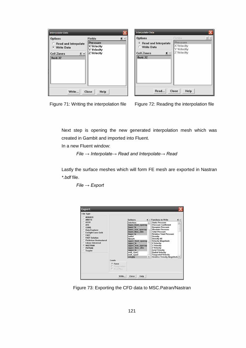
121

Figure 71: Writing the interpolation file

Figure 72: Reading the interpolation file

Next step is opening the new generated interpolation mesh which was

created in Gambit and imported into Fluent.

In a new Fluent window:

File → Interpolate→ Read and Interpolate→ Read

Lastly the surface meshes which will form FE mesh are exported in Nastran

*.bdf file.

File → Export

Figure 73: Exporting the CFD data to MSC.Patran/Nastran

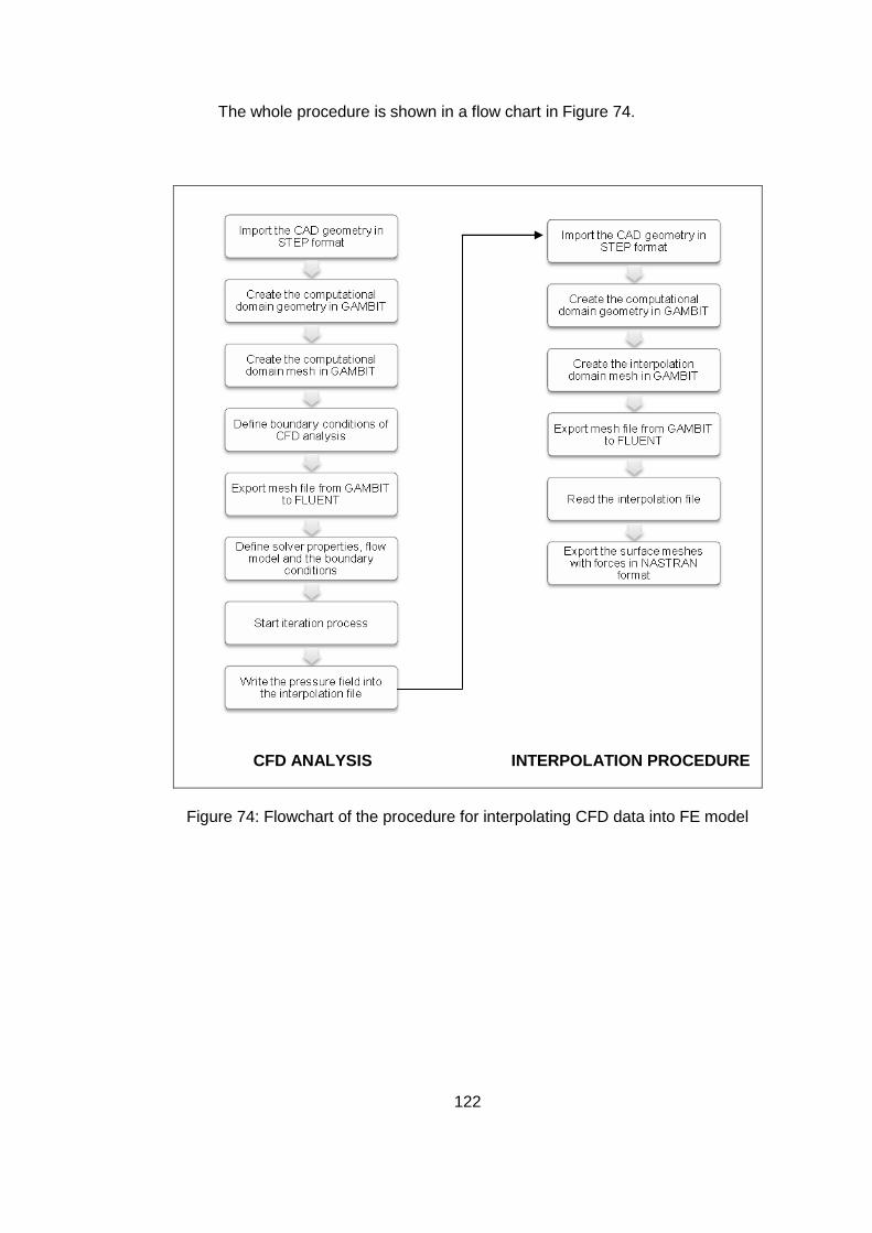
122

The whole procedure is shown in a flow chart in Figure 74.

CFD ANALYSIS INTERPOLATION PROCEDURE

Figure 74: Flowchart of the procedure for interpolating CFD data into FE model