Structural Complexity of Vortex Flows by Diagram Analysis and Knot Polynomials

Structural Complexity of Vortex Flowsby Diagram Analysis and KnotPolynomials

Renzo L. Ricca

Abstract In this paper I present and discuss with examples new techniques basedon the use of geometric and topological information to quantify dynamicalinformation and determine new relationships between structural complexity anddynamical properties of vortex flows. New means to determine linear and angularmomenta from standard diagram analysis of vortex tangles are provided, and theJones polynomial, derived from the skein relations of knot theory is introduced asa new knot invariant of topological fluid mechanics. For illustration severalexplicit computations are carried out for elementary vortex configurations. Thesenew techniques are discussed in the context of ideal fluid flows, but they can beequally applied in the case of dissipative systems, where vortex topology is nolonger conserved. In this case, a direct implementation of adaptive methods in areal-time diagnostics of real vortex dynamics may offer a new, powerful tool toanalyze energy-complexity relations and estimate energy transfers in highly tur-bulent flows. These methods have general validity, and they can be used in manysystems that display a similar degree of self-organization and adaptivity.

Keywords Euler equations � Linear and angular momenta � Diagram analysis �Vortex knots and links � Topological fluid dynamics � Structural complexity

R. L. Ricca (&)Department of Mathematics and Applications, University of Milano-Bicocca,Via Cozzi 53 20125 Milano, Italye-mail: [email protected]: www.matapp.unimib.it/*ricca/

R. L. RiccaKavli Institute for Theoretical Physics, UCSB Santa Barbara, California, USA

I. Zelinka et al. (eds.), How Nature Works, Emergence,Complexity and Computation 5, DOI: 10.1007/978-3-319-00254-5_5,� Springer International Publishing Switzerland 2014

81

1 Introduction

Networks of fluid structures, such as tangles of vortex filaments in turbulent flowsor braided magnetic fields in magnetohydrodynamics, are examples of physicalsystems that by their own nature are fundamentally structurally complex [1]. Thisis the result of many contributing factors, among which the highly nonlinearcharacter of the governing equations, the simultaneous presence of different spacescales in the emerging phenomena, and the spontaneous self-organization of theconstituent elements. In this respect ideal vortex dynamics offers a suitable the-oretical framework to develop and apply methods of structural complexity toinvestigate and analyze dynamical properties and energy-complexity relations.

In this paper I present and discuss with examples new techniques based on the useof algebraic, geometric and topological information to quantify dynamical infor-mation and to determine new relationships between energy and complexity incoherent vortex flows. These flows, that arise naturally from spontaneous self-organization of the vorticity field into thin filaments, bundles and tangles of filamentsin space, both in classical and quantum fluids, share common features, being the seedsand sinews of homogeneous, isotropic turbulence [2, 3]. Characterization andquantification of such flows is of fundamental importance from both a theoretical andapplied viewpoint. From a theoretical point of view detailed understanding of howstructural, dynamical and energetic properties emerge in the bulk of the fluid andchange both in space and in time is at the basis of our analysis of how self-organi-zation and non-linearities play their role in complex phenomena. For applications,understanding these aspects is also of fundamental importance to develop new real-time diagnostic tools to investigate and quantify dynamical properties of turbulentflows in classical fluid mechanics and magnetohydrodynamics.

The remarkable progress in the use of geometric and topological techniquesintroduced in the last decade [5–7], associated with continuous progress in com-putational power and visualization techniques [8, 9] in the light of the most recentdevelopments in the field [10], is a testimony of the success of this novel approach.Here we shall confine ourselves to some new geometric and topological techniquesintroduced recently [11, 12] to estimate dynamical properties of complex vortextangles of filaments in space. Most of the concepts presented here, being of geo-metric and topological origin, are independent of the actual physical model. Weshall therefore momentarily drop the physics, and refer to the geometry andtopology of the filament centerlines. These will be simply seen as smooth curvesthat may form knots, links and tangles in space, and it is to this system of curvesthat our analysis will be dedicated. Then, we shall apply this analysis to vortexdynamics, in order to get new physical information.

In Sect. 2 I start by introducing basic notions of standard and indented diagramprojections to determine signed area and crossing numbers of knots and links inspace. In Sect. 3 the definitions of linear and angular momenta of a vortex systemin ideal conditions are introduced, providing a geometric interpretation of thesequantities in terms of area. As illustration a number of examples are presented in

82 R. L. Ricca

Sect. 4 to evaluate the impetus of some vortex knots and links; a general statementon the signed area interpretation of the momenta for vortex tangles is presented inSect. 5. Then, in Sect. 6 knot polynomial invariants used to classify topologicallyclosed space curves in knot theory are considered. I concentrate on the Jonespolynomial, and, for illustration, the polynomial for several elementary knots andlinks (Sect. 7) are computed. By showing that it can be expressed in terms ofkinetic helicity (Sect. 8), I show that the Jones polynomial can be re-interpreted asa new invariant of topological fluid mechanics (Sect. 9). In Sect. 10 I concludewith some considerations on possible future implementations of these concepts inadvanced, adaptive, real-time diagnostics, to estimate energy and helicity transfersin real, turbulent flows.

2 Standard and Indented Diagrams: Signed Areasand Crossing Numbers of Knots and Links

To begin with, let us consider an isolated, oriented curve v in R3; this can be

thought of as the axis of a tubular neighborhood that constitute the support of theactual vortex filament in space; the orientation of the curve is then naturallyinduced by the orientation of vorticity. v is taken sufficiently smooth (i.e. at leastC2) and simple (without self-intersections), given by the position vector X ¼ XðsÞ,where s 2 ½0; L� is arc-length and L the total length. A Frenet triad ft; n; bg, givenby the unit tangent t ¼ dX=ds, normal and binormal vector, is defined on any pointof v and at each point of v curvature c ¼ cðsÞ and torsion s ¼ sðsÞ are defined.From the fundamental theorem of space curves, any curve in space is prescribeduniquely, once curvature and torsion are given as known functions of s. For thepurpose of this paper we confine ourselves to closed and possibly knotted curves.A closed curve is given by Xð0Þ ¼ XðLÞ and smooth closure implies that this isalso true for higher derivatives of XðsÞ.

Under continuous deformations the geometric properties of v change continu-ously, but the topological properties remain invariant. Any curve that can becontinuously deformed to the standard circle (without going through self-inter-sections or cuts) is not knotted and it is called the unknot. The task of knot theory(and of topology in general) is precisely to classify curves according to thetopological characteristics of their knot (or link) type, where a collection (disjointunion) of N such curves, knotted or unknotted, constitute a link. A link of twomathematical tubes, centered on the axes v1 and v2, is shown in Fig. 1a. A vortextangle is thus an N-component link of vortex filaments, where vorticity is simplydefined within the tubular neighborhood of each component.

Standard projection. Let us consider now the standard projection of an N-component link; for simplicity, let us take the case of the 2-component link ofFig. 1a, and consider the orthogonal projection p of this link onto the plane. Theresulting graph K ¼ pðv1 [ v2Þ is a nodal curve in R

2 with 4 intersection points

Structural Complexity of Vortex Flows by Diagram Analysis and Knot Polynomials 83

(Fig. 1b). Each nodal point results from the intersection of 2 incident (oriented)arcs: these nodal points have therefore multiplicity (or degree) 2. In general, anodal point of multiplicity l is the intersection of l incident arcs. By a smallperturbation of the projection map p, a l-degree point can be reduced to l nodalpoints of degree 2 (see the example of Fig. 2). A good, standard projection istherefore a map that for any link of curves generates a planar graph K, with at mostnodal points of degree 2. Let us restrict our attention to such good projections andconsider the graph K, given by a collections of oriented arcs.

Indented projection. Let us focus now on the topological characteristics of alink, for instance the 2-component link of Fig. 1a. One way to analyze topologicalaspects of a link is to consider indented projections. One of these is given byprojecting the link onto a plane by keeping track of the over/under-crossings bysmall indentations of the over/under-passes of the projected arcs (see the exampleof Fig. 1c). As above, we must ensure that at each apparent crossing only two arcsmeet.

Signed areas from standard projections. The graph K, obtained from standardprojections, determines a number of regions, say Rj (j ¼ 1; . . .; Z), in the plane.

(a)

(b) (c)

Fig. 1 a A 2-component link of tubes centered on the oriented curves v1 and v2 in space.b Standard projection of the link shown in (a) onto R

2; the resulting graph K ¼ pðv1 [ v2Þ is anoriented nodal curve in the plane, with 4 intersection points. c Indented projection of the samelink onto R

2: by small indentations in the plane, over-crossings and under-crossings are shown topreserve topological information of the original link in space

Fig. 2 A point P of multiplicity 3 can be reduced to 3 nodal points P1, P2, P3 of multiplicity(degree) 2

84 R. L. Ricca

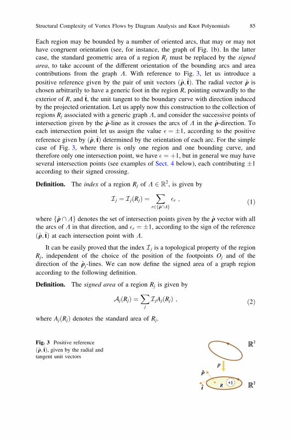
Each region may be bounded by a number of oriented arcs, that may or may nothave congruent orientation (see, for instance, the graph of Fig. 1b). In the lattercase, the standard geometric area of a region Rj must be replaced by the signedarea, to take account of the different orientation of the bounding arcs and areacontributions from the graph K. With reference to Fig. 3, let us introduce apositive reference given by the pair of unit vectors ðq; tÞ. The radial vector q ischosen arbitrarily to have a generic foot in the region R, pointing outwardly to theexterior of R, and t, the unit tangent to the boundary curve with direction inducedby the projected orientation. Let us apply now this construction to the collection ofregions Rj associated with a generic graph K, and consider the successive points ofintersection given by the q-line as it crosses the arcs of K in the q-direction. Toeach intersection point let us assign the value � ¼ �1, according to the positivereference given by ðq; tÞ determined by the orientation of each arc. For the simplecase of Fig. 3, where there is only one region and one bounding curve, andtherefore only one intersection point, we have � ¼ þ1, but in general we may haveseveral intersection points (see examples of Sect. 4 below), each contributing �1according to their signed crossing.

Definition. The index of a region Rj of K 2 R2, is given by

I j ¼ I jðRjÞ ¼X

r2fq\Kg�r ; ð1Þ

where fq \ Kg denotes the set of intersection points given by the q vector with allthe arcs of K in that direction, and �r ¼ �1, according to the sign of the referenceðq; tÞ at each intersection point with K.

It can be easily proved that the index I j is a topological property of the regionRj, independent of the choice of the position of the footpoints Oj and of thedirection of the qj-lines. We can now define the signed area of a graph regionaccording to the following definition.

Definition. The signed area of a region Rj is given by

AjðRjÞ ¼X

j

I jAjðRjÞ ; ð2Þ

where AjðRjÞ denotes the standard area of Rj.

Fig. 3 Positive referenceðq; tÞ, given by the radial andtangent unit vectors


The signed area extends naturally the concept of standard area for regionsbounded by arcs of different orientations and it will be useful in the geometricinterpretation of linear and angular momenta of vortex tangles.

Minimum number of crossings and linking number from indented projections.Two useful topological invariants can be extracted from indented projections. Oneis based on the minimum number of apparent crossings in an indented projection.Among the infinite number of possible indented projections, we consider theindented projection that gives the minimum number of crossings (minimal dia-gram) and, quite simply, we define this number as the topological crossing numberof the knot or link type.

Another topological quantity can be computed from a generic indented pro-jection. By standard convention (see Fig. 4) we assign �r ¼ �1 to each apparentcrossing site r. We can then introduce the following:

Definition. The linking number of a link type is given by

Lk ¼ 12

X

r

�r ; ð3Þ

where the summation is extended to all the apparent crossing sites, in any genericindented projection of the link.

In the example of Fig. 1c, there are 4 apparent crossings þ1, hence the linkingnumber Lkðv1; v2Þ ¼ þ2. Since the linking number is a topological invariant, itsvalue is independent from the projection.

3 Linear and Angular Momentum of a Vortex Tanglefrom Geometric Information

First, let us consider a single vortex filament K in an unbounded, ideal fluid at restat infinity, where vorticity is confined in the filament tube. Vortex filaments arisenaturally in superfluid turbulence [3], where indeed vorticity remains localized forvery long time on extremely thin filaments, with typical length of the order of 1 cmand vortex cross-section of the order of 10�8 cm.

Let K ¼ KðvÞ be centered on the filament axis v. Let us assume that vorticity isgiven simply by x ¼ x0 t, where x0 is a constant, and orientation is induced byvorticity. The vortex circulation (an invariant of the Euler’s equations, andquantized in the superfluid case), is given by

Fig. 4 Standard signconvention for a positive(over-) crossing and anegative (under-) crossing

86 R. L. Ricca

j ¼Z

Ax d2X ¼ constant; ð4Þ

where A is the area of the vortex cross-section. Two fundamental invariants ofideal fluid mechanics are the linear and angular momenta. The linear momentum(per unit density) P ¼ PðKÞ corresponds to the hydrodynamic impulse, which isnecessary to generate the motion of the vortex from rest; from its standard defi-nition [13], it takes the form

P ¼ 12

Z

VX� x d3X ¼ 1

2jI

LðvÞX� t ds ¼ constant; ð5Þ

where V is the filament volume. Similarly, for the angular momentum (per unitdensity) M ¼MðKÞ (the moment of the impulsive forces acting on K), given by

M ¼ 13

Z

VX� ðX� xÞ d3X ¼ 1

3jI

LðvÞX� ðX� tÞ ds ¼ constant: ð6Þ

Now evidently, since t ds ¼ dX, the right-hand-side integrals in (5) and (6) admitan interpretation in terms of (twice) the geometric area. It is quite surprising thatthis geometric interpretation, recognized by Lord Kelvin in his early works onvortex motion, has remained almost unexploited to date, and it is this particularaspect that we want to exploit here. Since both P and M are vector quantities, eachvector component can be related to the area of the graph resulting from theprojection of v along the direction of projection given by that component. Byreferring to the standard projection K ¼ pðvÞ, we have

pðvÞ : R3 ! R

2 ;

px : Kyz ; Ayz ¼ AðKyzÞ ;py : Kzx ; Azx ¼ AðKzxÞ ;pz : Kxy ; Axy ¼ AðKxyÞ ;

8><

>:ð7Þ

where, in the case of a simple, non-self-interesecting, planar curve K, Að�Þcoincides with the standard geometric area bounded by K. Hence, we can write

P ¼ ðPx;Py;PzÞ ¼ jðAyz;Azx;AxyÞ ; ð8Þ

M ¼ ðMx;My;MzÞ ¼23

jðdxAyz; dyAzx; dzAxyÞ ; ð9Þ

where dxAyz, dyAzx, dzAxy are the areal moments given according to the followingdefinition.

Definition. The areal moment around any axis is the product of the area Amultiplied by the distance d between that axis and the axis aG, normal to Athrough the centroid G of A.


Hence, dx, dy, dz denote the Euclidean distances of the area centroid G of Afrom the axes x, y, z, respectively.

4 Impetus of Vortex Knots and Links: Some Examples

4.1 Single-Component Systems: Vortex Knots

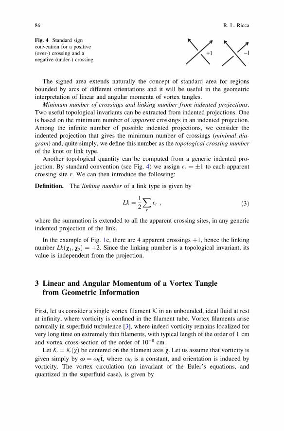
Figure-of-eight knot. Let us consider the diagram of Fig. 5a and let us evaluate theindices of the graphs. Suppose that this diagram results from the projection of afigure-of-eight knot (in the diagram shown we kept track of over-crossings andunder-crossings for visualization purposes only; in the standard, planar projectionall the crossings become nodal points). For each region we arbitrarily choose aradial vector and for each vector we consider the intersections of the q-line withthe graph. At each intersection we assign a þ1 or a �1, according to the positivereference defined in Sect. 2, and we sum up all the contributions according to (1),hence determining the index of that region. Their values are shown encircled inFig. 5a. These values are topological in character, because they do not depend onthe choice of the footpoint of q, thus providing the necessary prefactor for thestandard area. Using Eq. (8) we see that the central region of the figure-of-eightknot with index 0 does not contribute to the impetus in the direction normal to thisplane projection, whereas the nearby regions, with relative indices þ1;�1 and �2will tend to contribute to the motion in opposite directions. The index �2 asso-ciated with the smallest region, then, may compensate for a modest areacontribution.

Poloidal coil. Consider now the diagram of Fig. 5b, and suppose that thisresults from the projection of a poloidal coil in space. Since the central area hasindex þ1 and the external lobes have all indices �1, by (8) we see that theresulting impetus component may amount to a negative value (depending on the

(b)(a)

Fig. 5 a The figure-of-eight knot shown in an indented projection. In a standard plane projectionall the apparent crossings collapse to nodal points. The encircled values denote the indicesassociated with their respective regions. b A poloidal coil in a standard plane projection

88 R. L. Ricca

relative contributions from standard areas), giving rise to a backward motion in theopposite direction of the normal to the plane of projection. Such strange type ofmotion has been actually found by numerical simulation by Barenghi et al. in 2006[14], and confirmed by more recent work by Maggioni et al. [15].

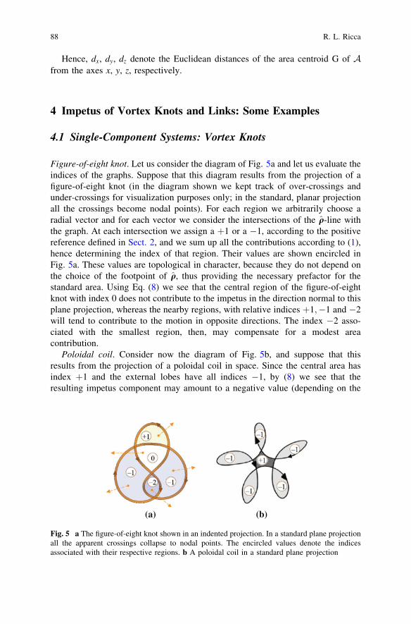
Trefoil knotting. A ‘‘thought experiment’’ to produce a trefoil vortex knot fromthe interaction and reconnection of vortex rings was conjectured by Ricca [16].Upon collision (see Fig. 6a), two vortex rings propagate one after the other toreconnect, thus forming a trefoil knot (as in Fig. 6b). By assigning the indices tothe different regions, it is possible to estimate the impulse associated with thedifferent parts of the vortex in relation to the projected areas.

4.2 Multi-Component Systems: Vortex Links

Rings. Two vortex rings of equal but opposite circulation move towards each otherto collide (see left diagram of Fig. 7). A finite number of reconnections take placeon the colliding vortices, triggering the production of smaller vortex rings. Smallrings are thus produced (right diagram of Fig. 7). This process has been actuallyrealized by head-on collision of coloured vortex rings in water by Lim & Nickels[17]. Since at the initial state linear momentum P ¼ 0 (for symmetry reason), weexpect that this remains so, till reconnections take place. The central diagram ofFig. 7 represents (schematically) the graph in the plane of collision, at thereconnection time. By applying the index computation, we can estimate the signedareas contributions. By using (8), we see that the central region does not contributeto the momentum of the system, whereas the outer regions, contribute withopposite sign to the momentum of the emerging small vortex rings. The alternatingsigns of the outer regions indicate the production of smaller rings of oppositepolarity, thus ensuring P ¼ 0 throughout the process. The generation and shoot-offof smaller rings from the plane of collision in opposite directions seems inagreement with the experimental results of Lim and Nickels [17].

Hopf links. Finally, let us consider the projection of a Hopf link made by twovortex rings of circulation j1 and j2 (see Fig. 8). All indices have same sign,

(a) (b)

Fig. 6 a Two vortex ring interact and b reconnect to form a trefoil knot. The central region,having largest area and highest index, is likely to move more rapidly than the rest of the system inthe normal direction to the projection plane


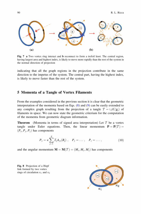
indicating that all the graph regions in the projection contribute in the samedirection to the impetus of the system. The central part, having the highest index,is likely to move faster than the rest of the system.

5 Momenta of a Tangle of Vortex Filaments

From the examples considered in the previous section it is clear that the geometricinterpretation of the momenta based on Eqs. (8) and (9) can be easily extended toany complex graph resulting from the projection of a tangle T ¼ [iKðviÞ offilaments in space. We can now state the geometric criterium for the computationof the momenta from geometric diagram information.

Theorem (Momenta in terms of signed area interpretation) Let T be a vortextangle under Euler equations. Then, the linear momentum P ¼ PðT Þ ¼ðPx;Py;PzÞ has components

Px ¼ jXZ

j¼1

I jAyzðRjÞ ; Py ¼ . . . ; Pz ¼ . . . ; ð10Þ

and the angular momentum M ¼MðT Þ ¼ ðMx;My;MzÞ has components

Fig. 8 Projection of a Hopflink formed by two vortexrings of circulation j1 and j2

(a) (b)

Fig. 7 a Two vortex ring interact and b reconnect to form a trefoil knot. The central region,having largest area and highest index, is likely to move more rapidly than the rest of the system inthe normal direction of projection

90 R. L. Ricca

Mx ¼23jdx

XZ

j¼1

I jAyzðRjÞ ; My ¼ . . . ; Mz ¼ . . . ; ð11Þ

where AyzðRjÞ, AzxðRjÞ, AxyðRjÞ denote the standard areas of Rjðj ¼ 1; . . .; ZÞ, forany projection plane normal to the component of the momenta of T .

Proof of the above Theorem is based on direct applications of (8), (9) and (2).

6 Knot Polynomial Invariants from Skein Relations:The Jones Polynomial

Indented diagrams of knot and link types are used to determine knot topology byextracting topological invariants known as knot polynomials. Several types of knotpolynomials have been introduced as subsequent improvements, R-polynomials,Kauffman brackets [18], Jones polynomials [19] and HOMFLY-PT [20, 21]polynomials being such types of knot invariants. These polynomials are deter-mined by skein relations derived from the analysis of crossing states in theindented diagrams of knots and links, given by un-oriented or oriented curves.With reference to Fig. 9, denoting by Lþ, L�, and L0 an over-crossing, an under-crossing and a non-crossing, respectively, we can derive skein relations for eachpolynomial.

6.1 Skein Relations of the Jones Polynomial

The Jones polynomial is a quite powerful knot invariant for oriented knots andlinks. It is therefore well-suited to tackle topological complexity of vortex tangles.The skein relations of the Jones polynomial are standardly derived by a techniquecalled local path-addition, that consists of computing crossing states according tothe analysis of the elementary states given by the over-crossing , theunder-crossing , and the disjoint union with a trivial circle. . Theskein relations of the Jones polynomial are given by [19, 22]:

ð12Þ

(a) (b) (c)

Fig. 9 a Over-crossingLþðþ1Þ, b under-crossingL�ð�1Þ, and c non-crossingL0 of oriented strands in anindented knot diagram


ð13Þ

Here we should stress that local path-additions are purely mathematical operations,performed virtually on the knot strands, the only purpose being simply themathematical derivation of the polynomial terms, that give rise to the desiredpolynomial invariant. No actual physical process is therefore involved.

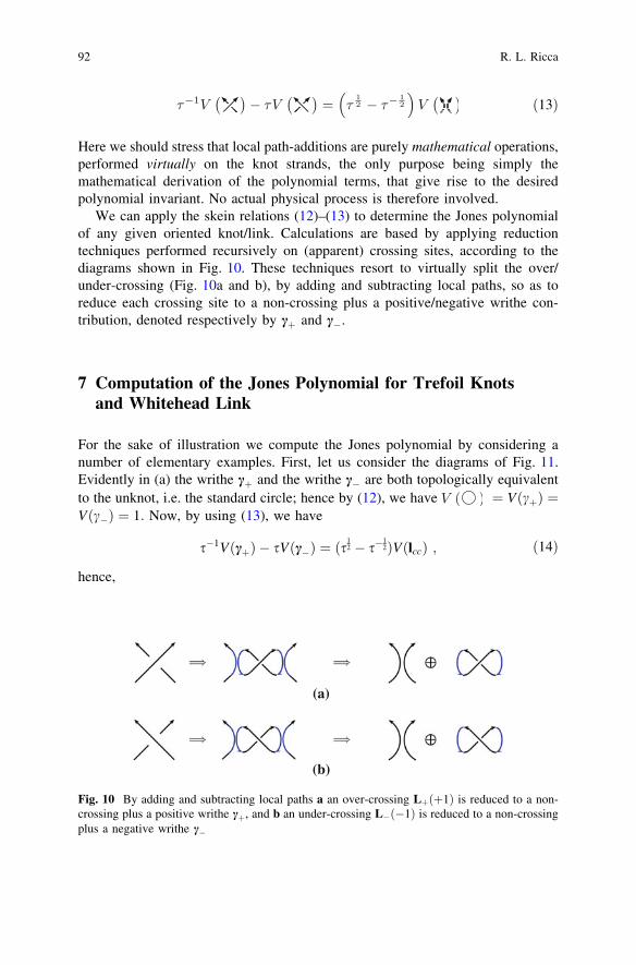
We can apply the skein relations (12)–(13) to determine the Jones polynomialof any given oriented knot/link. Calculations are based by applying reductiontechniques performed recursively on (apparent) crossing sites, according to thediagrams shown in Fig. 10. These techniques resort to virtually split the over/under-crossing (Fig. 10a and b), by adding and subtracting local paths, so as toreduce each crossing site to a non-crossing plus a positive/negative writhe con-tribution, denoted respectively by cþ and c�.

7 Computation of the Jones Polynomial for Trefoil Knotsand Whitehead Link

For the sake of illustration we compute the Jones polynomial by considering anumber of elementary examples. First, let us consider the diagrams of Fig. 11.Evidently in (a) the writhe cþ and the writhe c� are both topologically equivalentto the unknot, i.e. the standard circle; hence by (12), we have ¼ VðcþÞ ¼Vðc�Þ ¼ 1: Now, by using (13), we have

s�1VðcþÞ � sVðc�Þ ¼ ðs12 � s�

12ÞVðlccÞ ; ð14Þ

hence,

(a)

(b)

Fig. 10 By adding and subtracting local paths a an over-crossing Lþðþ1Þ is reduced to a non-crossing plus a positive writhe cþ, and b an under-crossing L�ð�1Þ is reduced to a non-crossingplus a negative writhe c�

92 R. L. Ricca

VðlccÞ ¼ �s�12 � s

12 : ð15Þ

Note that the orientation of any number of disjoint rings has no effect on thepolynomial. As regards to the Hopf link Hþ (Fig. 11b), we have

s�1VðHþÞ � sVðlccÞ ¼ ðs12 � s�

12ÞVðcþÞ ; ð16Þ

that gives

VðHþÞ ¼ �s12 � s

52 : ð17Þ

Similarly for the Hopf link H� of Fig. 11c:

s�1VðlccÞ � sVðH�Þ ¼ ðs12 � s�

12ÞVðc�Þ ; ð18Þ

that gives

VðH�Þ ¼ �s�12 � s�

52 : ð19Þ

7.1 Left-Handed and Right-Handed Trefoil Knots

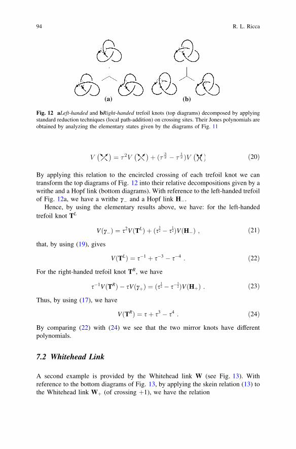
The left-handed trefoil knot TL and right-handed trefoil knot TR are shown by thetop diagrams of Fig. 12a and b, respectively. By re-arranging (13), we can converta crossing in terms of its opposite plus a contribution from parallel strands, that is

(a)

(b)

(c)

Fig. 11 a Writhes cþ, c� and disjoint union of two trivial circles lcc. b Hopf link Hþ withcrossing þ1, disjoint union of circles lcc and writhe cþ. c Hopf link H� with crossing �1, disjointunion of circles lcc and writhe c�. Note that the orientation of any number of disjoint circles doesnot influence the polynomial


ð20Þ

By applying this relation to the encircled crossing of each trefoil knot we cantransform the top diagrams of Fig. 12 into their relative decompositions given by awrithe and a Hopf link (bottom diagrams). With reference to the left-handed trefoilof Fig. 12a, we have a writhe c� and a Hopf link H�.

Hence, by using the elementary results above, we have: for the left-handedtrefoil knot TL

Vðc�Þ ¼ s2VðTLÞ þ ðs32 � s

12ÞVðH�Þ ; ð21Þ

that, by using (19), gives

VðTLÞ ¼ s�1 þ s�3 � s�4 : ð22Þ

For the right-handed trefoil knot TR, we have

s�1VðTRÞ � sVðcþÞ ¼ ðs12 � s�

12ÞVðHþÞ : ð23Þ

Thus, by using (17), we have

VðTRÞ ¼ sþ s3 � s4 : ð24Þ

By comparing (22) with (24) we see that the two mirror knots have differentpolynomials.

7.2 Whitehead Link

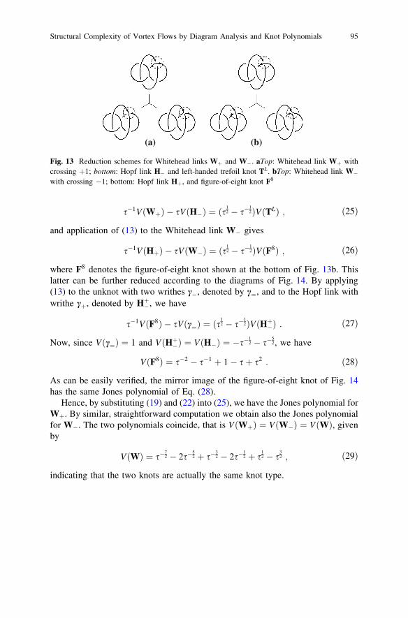
A second example is provided by the Whitehead link W (see Fig. 13). Withreference to the bottom diagrams of Fig. 13, by applying the skein relation (13) tothe Whitehead link Wþ (of crossing þ1), we have the relation

(a) (b)

Fig. 12 aLeft-handed and bRight-handed trefoil knots (top diagrams) decomposed by applyingstandard reduction techniques (local path-addition) on crossing sites. Their Jones polynomials areobtained by analyzing the elementary states given by the diagrams of Fig. 11

94 R. L. Ricca

s�1VðWþÞ � sVðH�Þ ¼ ðs12 � s�

12ÞVðTLÞ ; ð25Þ

and application of (13) to the Whitehead link W� gives

s�1VðHþÞ � sVðW�Þ ¼ ðs12 � s�

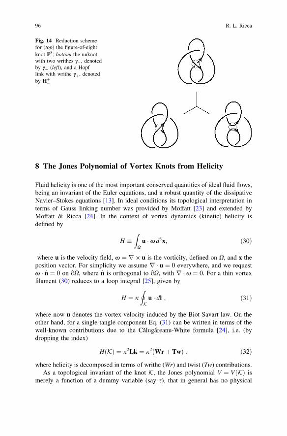
12ÞVðF8Þ ; ð26Þ

where F8 denotes the figure-of-eight knot shown at the bottom of Fig. 13b. Thislatter can be further reduced according to the diagrams of Fig. 14. By applying(13) to the unknot with two writhes c�, denoted by c¼, and to the Hopf link withwrithe cþ, denoted by Hþ�, we have

s�1VðF8Þ � sVðc¼Þ ¼ ðs12 � s�

12ÞVðHþ�Þ : ð27Þ

Now, since Vðc¼Þ ¼ 1 and VðHþ�Þ ¼ VðH�Þ ¼ �s�12 � s�

52, we have

VðF8Þ ¼ s�2 � s�1 þ 1� sþ s2 : ð28Þ

As can be easily verified, the mirror image of the figure-of-eight knot of Fig. 14has the same Jones polynomial of Eq. (28).

Hence, by substituting (19) and (22) into (25), we have the Jones polynomial forWþ. By similar, straightforward computation we obtain also the Jones polynomialfor W�. The two polynomials coincide, that is VðWþÞ ¼ VðW�Þ ¼ VðWÞ, givenby

VðWÞ ¼ s�72 � 2s�

52 þ s�

32 � 2s�

12 þ s

12 � s

32 ; ð29Þ

indicating that the two knots are actually the same knot type.

(b)(a)

Fig. 13 Reduction schemes for Whitehead links Wþ and W�. aTop: Whitehead link Wþ withcrossing þ1; bottom: Hopf link H� and left-handed trefoil knot TL. bTop: Whitehead link W�with crossing �1; bottom: Hopf link Hþ, and figure-of-eight knot F8


8 The Jones Polynomial of Vortex Knots from Helicity

Fluid helicity is one of the most important conserved quantities of ideal fluid flows,being an invariant of the Euler equations, and a robust quantity of the dissipativeNavier–Stokes equations [13]. In ideal conditions its topological interpretation interms of Gauss linking number was provided by Moffatt [23] and extended byMoffatt & Ricca [24]. In the context of vortex dynamics (kinetic) helicity isdefined by

H �Z

Xu � x d3x; ð30Þ

where u is the velocity field, x ¼ r� u is the vorticity, defined on X, and x theposition vector. For simplicity we assume r � u ¼ 0 everywhere, and we requestx � n ¼ 0 on oX, where n is orthogonal to oX, with r � x ¼ 0. For a thin vortexfilament (30) reduces to a loop integral [25], given by

H ¼ jI

Ku � dl ; ð31Þ

where now u denotes the vortex velocity induced by the Biot-Savart law. On theother hand, for a single tangle component Eq. (31) can be written in terms of thewell-known contributions due to the Calugareanu-White formula [24], i.e. (bydropping the index)

HðKÞ ¼ j2Lk ¼ j2ðWrþ TwÞ ; ð32Þ

where helicity is decomposed in terms of writhe (Wr) and twist (Tw) contributions.As a topological invariant of the knot K, the Jones polynomial V ¼ VðKÞ is

merely a function of a dummy variable (say s), that in general has no physical

Fig. 14 Reduction schemefor (top) the figure-of-eightknot F8; bottom the unknotwith two writhes c�, denotedby c¼ (left), and a Hopflink with writhe cþ, denotedby Hþ�

96 R. L. Ricca

meaning: thus VðKÞ ¼ VsðKÞ. Since in our case K is a vortex knot, during evo-lution it carries topological as well as dynamical information. Following [12], wecan encapsulate this dual property by combining the two Eqs. (31) and (32) intothe variable s (by an appropriate transformation), showing that this new s satisfiesthe skein relations of the Jones polynomial. Indeed, by using (31) and (32) and thetransformation eH ! tH ! s, we have the following [12]:

Theorem ([12]): Let K denote a vortex knot (or an N-component link) of helicityH ¼ HðKÞ. Then

tHðKÞ ¼ tHK

u�dl; ð33Þ

appropriately re-scaled, satisfies (with a plausible statistical hypothesis) the skeinrelations of the Jones polynomial V ¼ VðKÞ.

Full proof of the above Theorem is given in the reference above, where theskein relations are derived in terms of the variable

s ¼ t�4kHðcþÞ ; k 2 ½0; 1� ; ð34Þ

where k takes into account the uncertainty associated with the writhe value of cþ(see the first diagram of Fig. 11a) and HðcþÞ denotes the helicity associated withcþ [12].

9 The Jones Polynomial as a New Fluid Dynamical KnotInvariant

For practical applications it is useful to go back to the original position, i.e.s! tH ! eH , by referring to eH rather than s. By (34) we can write knot poly-nomials for a vortex tangle of filaments as function of topology and HðcþÞ, wherethe latter can be interpreted as a reference mean-field helicity of the physicalsystem. Indeed, by (32), we can think of HðcþÞ as a gauge for a mean writhe (ortwist) helicity of the background flow. Since in any case this contributes in termsof an average circulation j, we can re-interpret the Jones polynomial as a newinvariant of topological fluid dynamics, i.e.

VsðKÞ ! VtðK; jÞ ! VðK; jÞ : ð35Þ

In the case of a homogeneous, isotropic tangle of superfluid filaments, all vorticeshave same circulation j; thus, by normalizing the circulation in dimensionlessform, we can set

�k ¼ hki ¼ 12; hHðcþÞi ¼

j2

2; ð36Þ


where angular brackets denote average values. Hence,

s ¼ t�j2 ! e�j2: ð37Þ

In this case, we have

ð38Þ

VðlccÞ ¼ �ej22 ð1þ e�j2Þ ; ð39Þ

Vðlc;...;cÞ ¼ ½�ej22 ð1þ e�j2Þ�N�1 ; ðN vortex ringsÞ ; ð40Þ

VðHþÞ ¼ �e�j2

2 ð1þ e�2j2Þ ; ð41Þ

VðH�Þ ¼ �ej22 ð1þ e2j2Þ ; ð42Þ

VðTLÞ ¼ ej2 þ e3j2 � e4j2; ð43Þ

VðTRÞ ¼ e�j2 þ e3j2 � e�4j2: ð44Þ

VðF8Þ ¼ e2j2 � ej2 þ 1� e�j2 þ e�2j2; ð45Þ

VðWÞ ¼ e�32j

2 �1þ ej2 � 2e2j2 þ e3j2 � 2e4j2 þ e5j2� �

: ð46Þ

These results are obtained by straightforward application of the transformation(37) to the computations carried out in Sect. 7. For more complex physical systemsknot polynomials can be straightforwardly computed by implementing skeinrelations and diagram analysis into a numerical code.

10 Concluding Remarks

Complex tangles of vortex filaments are ubiquitous in turbulent flows, and are keyfeatures of homogeneous isotropic turbulence in both classical and quantum sys-tems. Detecting their structural complexity and attempting to relate complexity todynamical and energetic properties are of fundamental importance for both theo-retical and practical reasons. Moreover, vortex tangles represent a good paradig-matic example of complex systems displaying features of self-organization andadaptive behavior largely independent of the space scale of the phenomena; theytherefore offer a perfect test case to study and tackle aspects of structural com-plexity in general.

98 R. L. Ricca

In this paper I reviewed new results obtained following an approach based onthe exploitation of geometric and topological information. Preliminary informationon standard and indented diagrams have been given in Sect. 2. Then, a newmethod to compute linear and angular momenta of a tangle of vortex filaments inideal fluids has been presented (Sects. 3 and 4). This method relies on the directinterpretation of these quantities in terms of geometric information (Sect. 5).Indeed, the technique proposed here is based on a rather straightforward analysisof planar graphs, and its direct implementation to analyze highly complex net-works seems amenable to more sophisticated improvements. Similar consider-ations hold for the implementation of skein relations to quantify topologicalproperties by knot polynomials, introduced in Sects. 6 and 7. Here, our attentionhas been restricted to the Jones polynomial, and its interpretation in terms of thehelicity of fluid flows (Sect. 8). This, in turn, has led us to re-consider and presentthis polynomial as a new invariant of ideal fluid mechanics, and a number ofelementary examples have been presented to demonstrate both the straightforwardapplication of computational techniques associated with the implementation of therelative skein relations, and the possibility to extend this approach to more com-plex systems (Sect. 9).

These results can be extended to real fluid flows as well. For these systemsviscosity play an important role, by producing continuous changes in the tangletopology, leading to the gradual dissipation of all conserved quantities, momenta,helicity and, of course, energy. This is certainly reflected in the continuous changeof geometric, topological and dynamical properties. Therefore, a real-timeimplementation of an adaptive analysis that takes account of these changes canprovide a useful tool for real-time diagnostics of the exchange and transfer ofdynamical properties and energy between different regions in the fluid. This,together with an adaptive, real-time implementation of a whole new set of mea-sures of structural complexity based on algebraic, geometric and topologicalinformation [25–27] will prove useful to investigate and tackle open problems inclassical, quantum and magnetic fluid flows, as well as in many other systems thatdisplay similar features of self-organization.

Acknowledgments This author wishes to thank the Kavli Institute for Theoretical Physics at UCSanta Barbara for the kind hospitality. This research was supported in part by the NationalScience Foundation under Grant No. NSF PHY11-25915.

References

1. R.L. Ricca, Structural Complexity, in Encyclopedia of Nonlinear Science, ed. by A. Scott(Routledge, New York, 2005), pp. 885–887

2. M.A. Uddin, N. Oshima, M. Tanahashi, T. Miyauchi, A study of the coherent structures inhomogeneous isotropic turbulence. Proc. Pakistan Acad. Sci. 46, 145–158 (2009)

3. A.I. Golov, P.M. Walmsley, Homogeneous turbulence in superfluid 4He in the low-temperature limit: experimental progress. J. Low Temp. Phys. 156, 51–70 (2009)


4. A.W. Baggaley, C.F. Barenghi, A. Shukurov, Y.A. Sergeev, Coherent vortex structures inquantum turbulence. EPL 98, 26002 (2012)

5. V.I. Arnold, B.A. Khesin, Topological Methods in Hydrodynamics. Applied MathematicalSciences, vol. 125, (Springer, Berlin, 1998)

6. R.L. Ricca, (ed.), An Introduction to the Geometry and Topology of Fluid Flows. NATO ASISeries II, vol. 47 (Kluwer, Dordrecht, 2001)

7. R.L. Ricca (ed.), Lectures on Topological Fluid Mechanics. Springer-CIME Lecture Notes inMathematics 1973 (Springer, Heidelberg, 2009)

8. J. Weickert, H. Hagen (eds.), Visualization and Processing of Tensor Fields (Springer,Heidelberg, 2006)

9. H. Hauser, H. Hagen, H. Theisel (eds.), Topology-based Methods in Visualization (Springer,Heidelberg, 2007)

10. H.K. Moffatt, K. Bajer, Y. Kimura (eds.), Topological Fluid Dynamics: Theory andApplications (Elsevier, 2013 )

11. R.L. Ricca, Momenta of a vortex tangle by structural complexity analysis. Physica D 237,2223–2227 (2008)

12. X. Liu, R.L. Ricca, The Jones polynomial for fluid knots from helicity. J. Phys. A: Math. &Theor. 45, 205501 (2012)

13. P.G. Saffman, Vortex Dynamics (Cambridge University Press, Cambridge, 1991)14. C.F. Barenghi, R. Hänninen, M. Tsubota, Anomalous translational velocity of vortex ring

with finite-amplitude Kelvin waves. Phys Rev. E 74, 046303 (2006)15. F. Maggioni, S.Z. Alamri, C.F. Barenghi, R.L. Ricca, Velocity, energy, and helicity of vortex

knots and unknots. Phys. Rev. E 82, 026309 (2010)16. R.L. Ricca, New developments in topological fluid mechanics. Nuovo Cimento C 32,

185–192 (2009)17. T.T. Lim, T.B. Nickels, Instability and reconnection in head-on collision of two vortex rings.

Nature 357, 225–227 (1992)18. L.H. Kauffman, On Knots (Princeton University Press, Princeton, 1987)19. V.F.R. Jones, Hecke algebra representations of braid groups and link polynomials. Ann.

Math. 126, 335–388 (1987)20. P. Freyd, D. Yetter, J. Hoste, W.B.R. Lickorish, K. Millett, A. Ocneanu, A new polynomial

invariant of knots and links. Bull. Am. Math. Soc. 12, 239–246 (1985)21. J.H. Przytycki, P. Traczyk, Conwav algebras and skein equivalence of links. Proc. Amer.

Math. Soc. 100, 744–748 (1987)22. L.H. Kauffman, Knots and Physics (World Scientific Publishing Co., Singapore, 1991)23. H.K. Moffatt, The degree of knottedness of tangled vortex lines. J. Fluid Mech. 35, 117–129

(1969)24. H.K. Moffatt, R.L. Ricca, Helicity and the Calugareanu invariant. Proc. R. Soc. A 439,

411–429 (1992)25. C.F. Barenghi, R.L. Ricca, D.C. Samuels, How tangled is a tangle? Physica D 157, 197–206

(2001)26. R.L. Ricca, On simple energy-complexity relations for filament tangles and networks.

Complex Syst. 20, 195–204 (2012)27. R. Ricca, New energy and helicity lower bounds for knotted and braided magnetic fields.

Geophys. Astrophys. Fluid Dyn. Online. doi:10.1080/03091929.2012.681782

100 R. L. Ricca

http://dx.doi.org/10.1080/03091929.2012.681782

Structural Complexity of Vortex Flows by Diagram Analysis and Knot Polynomials

Documents

Transcript of Structural Complexity of Vortex Flows by Diagram Analysis and Knot Polynomials