Structural Change and Homeostasis in Organizations: A ...
34
Structural Change and Homeostasis in Organizations: A Decision-Theoretic Approach 12 Carter T. Butts 3 Kathleen M. Carley 4 February 21, 2005 Word Count: 8612 Running Head: STRUCTURAL CHANGE AND HOMEOSTASIS IN ORGANIZATIONS 1 This work was supported in part by the Office of Naval Research (ONR), United States Navy Grant No. 1681-1-1001944, by the Army Research Labs on the grant “Personnel Turnover and Team Performance,” by the National Science Foundation under Grants No. ITR/IM IIS-0081219, ITR IIS-0331707, and IGERT Grant No. 9972762, and by the center for Computational Analysis of Social and Organizational Systems (CASOS) at Carnegie Mellon University. The views and conclusions contained in this document are those of the authors and should not be interpreted as representing the official policies, either expressed or implied, of the Office of Naval Research, the Army Research Labs, the National Science Foundation, or the U.S. government. 2 The authors would like to thank David Rode for his helpful comments regarding this paper. 3 Department of Sociology and Institute for Mathematical Behavioral Sciences; University of California, Irvine; Irvine, CA 92697; [email protected] 4 Institute for Software Research International, School of Computer Science and Center for the Compu- tational Analysis of Social and Organizational Systems, Carnegie Mellon University
Transcript of Structural Change and Homeostasis in Organizations: A ...
Structural Change and Homeostasis in Organizations: A
Decision-Theoretic Approach1 2
Carter T. Butts3 Kathleen M. Carley4
February 21, 2005
Word Count: 8612
Running Head: STRUCTURAL CHANGE AND HOMEOSTASIS IN ORGANIZATIONS
1This work was supported in part by the Office of Naval Research (ONR), United States Navy Grant No.
1681-1-1001944, by the Army Research Labs on the grant “Personnel Turnover and Team Performance,”
by the National Science Foundation under Grants No. ITR/IM IIS-0081219, ITR IIS-0331707, and IGERT
Grant No. 9972762, and by the center for Computational Analysis of Social and Organizational Systems
(CASOS) at Carnegie Mellon University. The views and conclusions contained in this document are those
of the authors and should not be interpreted as representing the official policies, either expressed or implied,
of the Office of Naval Research, the Army Research Labs, the National Science Foundation, or the U.S.
government.2The authors would like to thank David Rode for his helpful comments regarding this paper.3Department of Sociology and Institute for Mathematical Behavioral Sciences; University of California,
Irvine; Irvine, CA 92697; [email protected] for Software Research International, School of Computer Science and Center for the Compu-
tational Analysis of Social and Organizational Systems, Carnegie Mellon University

Abstract
We present here a decision-theoretic framework for the analysis of organizational change and home-
ostasis under risk. An algorithm is demonstrated which identifies optimal change paths given uncer-
tainty involving execution time, intervention cost, and payoffs resulting from particular structural
configurations. An elaboration of the basic framework to accommodate external structural pertur-
bations is shown, and is applied to the problem of organizational homeostasis. Finally, an extension
of the decision model is provided which admits multiple decision makers with divergent preferences
and capacities for inducing organizational change.
Keywords: organizational design, structural change, network evolution, decision theory, homeosta-
sis, organizational adaptation, dynamic network analysis

STRUCTURAL CHANGE AND HOMEOSTASIS IN ORGANIZATIONS 1
1 Introduction
Organizations are not unitary, undifferentiated entities: each is composed of an assortment of lower
level components (human actors, physical resources, tasks to be performed, etc.), components
which are in some particular configuration with respect to one another at any given time (Carley,
2002b;a). Furthermore, the performance and survival of an organization is contingent (at least
in part) on the configuration of its parts (see e.g., Thompson, 1967; Perrow, 1970; Pfeffer and
Salancik, 1978; Galbraith, 1977). Research over the past three decades has indicated that there is
no globally optimal organizational design (Blau, 1972; Mackenzie, 1978; Lincoln et al., 1986; Lin,
1994); however, this work also suggests that locally optimal organizational forms may be found for
particular task structures and environmental contexts (Williamson, 1975; Duncan, 1979; Burton
and Obel, 1984; Baligh et al., 1990; Crowston, 1994; Levchuk et al., 2002a;b). This research points
to a fundamental question: given a particular starting point, how can an organization restructure
itself over time to reach a (locally) optimal form?
In this paper, we focus on the process by which an organization is moved from an initial state to
a “target” design. We take an explicitly decision-theoretic point of view, identifying an optimal path
to the target state under a specified payoff regime. The ultimate purpose of this exercise is three-
fold. Our first purpose is to contribute to the sociological literature on change in organizations, by
providing a baseline against which to compare actual change processes. Just as the rational actor
model has proven consistently useful in the psychology of individual judgment and decision making
(Tversky and Kahneman, 1986; Dawes, 1996), so too have optimization-based models contributed
to the theory of organizations (Arrow, 1974; Williamson, 1975; Glance and Huberman, 1994). By
examining deviations from optimal change behavior, we may illuminate the sorts of processes that
govern real structural shifts; similarly, by means of our decision model, we may predict the effects
of heuristic decision processes on organizational performance. Second, by demonstrating how the
optimal change problem may be formulated (and, in some cases, solved) as a decision problem,
we hope to contribute to the normative (i.e., social or organizational engineering) literature on
STRUCTURAL CHANGE AND HOMEOSTASIS IN ORGANIZATIONS 2
organizational design. This work builds on traditional approaches that either pre-define the possible
paths of change (e.g., Perdu and Levis, 1998), optimize end states without discussing the change
path (e.g., Levchuk et al., 2000), or limit consideration to fixed structural representations and/or
omit dynamic properties related to the pace of change (Levchuk et al., 2004). Finally, the third
purpose of the present work is to provide a formal basis for further work on “structural games;”
i.e., the strategic interactions among multiple stakeholders involved in determining the evolution
of a complex organization. By viewing organizational change through a decision-theoretic lens, we
highlight both normative and descriptive aspects of organizational change and homeostasis.
2 Concepts and Definitions
Before proceeding to the decision problem itself, we begin by setting out some basic concepts. These
consist of representations for the organizational structures themselves, the transformations that will
be used to take one structure into another (i.e., interventions), and payoffs to the Organizational
Designer, respectively. Throughout, our approach will be to emphasize generality over problem-
specificity; by maintaining a high level of abstraction, we hope to provide the widest possible scope
for the methods described herein.
2.1 Organizational Structure
In order to provide a decision-theoretic framework for organizational change, we must first set
forth a concrete representation of organizational structure. Following prior research in this area,
we define structure in terms of the meta-matrix connecting relevant components such as personnel,
knowledge and tasks (Carley and Krackhardt, 1998; 1999; Carley and Hill, 2001; Carley, 2002a;
Carley et al., 2003). As such, the structure of any given organization, ζ, is a collection of graphs;
we make no further assumptions about the nature of the structures in question (e.g., whether the
graphs are simple, directed, valued, etc.).1 Such a structure is, in turn, taken to be a member of a1In fact, even this assumption is not required for any of the formal results shown here; these depend only on the
properties of the constructs G, T, and π (see below). Our discussion of potential structural payoff functions and our

STRUCTURAL CHANGE AND HOMEOSTASIS IN ORGANIZATIONS 3
much larger set of structures which could in principle be occupied by ζ. More formally:
Definition 1. Given an organization ζ composed of graphs G1, . . . , Gn, we refer to G = {G1, . . . , Gn}
as the structure set of ζ. The set of all realizable G is in turn represented by G, the structural
universe of ζ.
Note that by “realizable” structure sets, we mean those that are in fact available to the orga-
nization, subject to its definitional constraints. Thus, if we defined organizational structure purely
in terms of reporting and task assignment relations, then all elements of G would be constrained
to have two members. For convenience, we may also (without loss of generality)2 take all G ∈ G
to have the same vertex set (though vertex sets may of course vary with G). Though this last is
not a requirement for the framework considered here, it does simplify matters considerably, and is
recommended in practice.
2.2 Structural Transformations
Having established a set of potential structures from which the current state of an organization may
be drawn, we now require a generic means of describing changes in that state. This is accomplished
via the notion of the structural transformation, which takes the set of structures into itself:
Definition 2. Any T : G → G is said to be a structural transformation for the structural universe
G. The set of all realizable, distinct structural transformations is denoted by the transformation
universe T.
Once again, the “realizability” of the elements of T is taken to refer to their empirical feasibility
in the context of the structural universe at hand. Thus, in a typical case, realizable structural
transformations might include the expansion or contraction of the vertex set (e.g., hiring/acquisition
or firing/liquidation), edge addition or deletion (e.g., task or personnel reassignment), etc. For
examples, however, do assume this.2Vertices intrinsically uninvolved in a given relation (e.g., knowledge elements in a task assignment network) can
simply be regarded as isolates for that relation.
STRUCTURAL CHANGE AND HOMEOSTASIS IN ORGANIZATIONS 4
the moment, we will consider T as unitary, in the sense that it represents the capability of a
single abstract decision maker (the hypothetical “Organizational Designer”) to alter organizational
structure. Later, we shall complicate this picture somewhat by assuming that transformations may
arise from more than one source, one of the most important being Chance.
The foregoing formalism does not consider a key element of transformation, i.e., time. In
general, structural change is not instantaneous: rather there is a period of implementation between
the decision to change and the realization of that change. This delay is significant since time spent
in a sub-optimal configuration can result in lost earnings, higher production costs, or worse. Taking
time into account, we introduce a function that given a transformation returns the time required
for the transformation to be implemented.3 Formally:
Definition 3. The time interval between the initiation of a structural transformation T and its
completion (i.e., the realization of T (G)) is referred to as the implementation time of T , and is
denoted ∆(T ).
Before moving ahead to a consideration of payoffs, we pause to combine the ideas of Definitions 1
and 2 into a single formalism. This formalism provides a useful shorthand for discussing the
structural changes – particularly sequences of such changes – and will be used extensively in the
discussion which follows. Taking the set of possible structures (the structural universe) together
with the set of feasible transformations (the transformation universe), we form a multi-graph that
encodes the complete set of changes that could be made by the organization in question. By
focusing on properties of this graph – rather than on the details of the particular elements of G
and T – we can more easily study the properties of potential structural changes.
Definition 4. Given a transformation T and structural universe G, the change graph (denoted GT )
of T on G is the graph formed by
(G, {(G, T (G))∀G ∈ G}). The collection of such graphs for all T ∈ T is then the change multi-3Note that we assume here that implementation time is a function of the structural transformation, and not of
the structure on which this transformation operates.

STRUCTURAL CHANGE AND HOMEOSTASIS IN ORGANIZATIONS 5
graph of T on G, denoted GT. A walk from Gα to Gω in GT is said to be a change walk, and if all
vertices of such a walk are distinct, the walk is further said to be a change path.
To foreshadow what we shall see in the coming sections, it is the change walk (or, ultimately, the
change path) which will be at the center of our attention. Intuitively, the change walk corresponds
to a particular strategy for converting an organization from an initial form (Gα) to a final one (Gω)
by means of a series of concrete interventions. Each such walk corresponds to a series of intermediate
positions occupied by the organization during the change process: observe that any change walk
from Gα to Gω can be written either in terms of a vertex sequence (i.e., Gα,Gβ , . . . ,Gω) or in
terms of an initial point together with a series of transformations (i.e., Gα, T1, . . . , Tn).4 This follows
from the fact that Gα,Gβ, . . . ,Gω = Gα, T1(Gα), . . . , Tn(· · · (T1(Gα))) (itself a consequence of the
definition of GT). This simple duality will be of use for the arguments that follow.
2.3 Payoff Functions
In the context of an organizational design problem, it is assumed that there exists some decision
maker who A) is able to act in altering organizational structure, and B) possesses well-formed
preferences regarding the structures in question. While real-world organizations generally possess
multiple stakeholders whose preferences are not entirely consistent with one another, we will initially
limit ourselves to the simpler case. To represent this decision maker’s preferences, we employ a
payoff function whose value is to be maximized. This function may be either of transformations or
of structural configurations, as indicated below:
Definition 5. Let π(T ) represent the partial payoff to the decision maker associated with employing
transformation T , and let π(G) be defined such that the partial payoff to the decision maker
associated with the organization ζ occupying state G for duration t is equal to tπ(G) for all t,G.4The astute reader will note that these representations are not precisely equivalent, in the sense that there may be
more than one transformation connecting each pair of adjacent structures. That this discrepancy is of no consequence
for the decision problem is shown below.
STRUCTURAL CHANGE AND HOMEOSTASIS IN ORGANIZATIONS 6
For the purposes of our analyses, we take all partial payoffs to be additive in transformations and
time: thus the partial payoff associated with employing transformations T1 and T2 is π (T1, T2) =
π (T1) + π (T2), and the partial payoff resulting from occupying states G1 and G2 for durations t1
and t2 (respectively) would be t1π (G1) + t2π (G2). Total payoffs, then, are further assumed to be
given by the sum of all partial payoffs. Thus, if our above scenarios were combined, the total payoff
to the organizational designer would be π (T1) + π (T2) + t1π (G1) + t2π (G2). Such an assumption
seems a plausible first approximation, and buys considerable economy in terms of the tractability of
the decision problem. Nonlinearly interacting payoff elements are left as a topic for future research.
It should be noted that an important task in defining the change decision problem is the
identification of the payoff functions described above. Determination of π(G), in particular, may
be nontrivial. One potential candidate for such a payoff function may be derived as follows. Let
f1, . . . , fm be a collection of structural indices such that fi : G → R ∀ G ∈ G. Then, let f∗1 , . . . , f∗m
represent optimal values for these indices. Given this, a structural payoff function could reasonably
take the form
π(G) =m∑
i=1
βig(f∗i − fi (G)
)(1)
where β is an a priori weight, and g is any decreasing even function (e.g., −x2, −|x|). Such
a payoff function corresponds to the idea that there exists an attribute space (provided by the
indices) containing some point such that distance from it is associated with decreasing payoffs. A
related – and even simpler – family of functions is given by
π(G) =m∑
i=1
βig(fi (G)
)(2)
that would be appropriate for linearly separable payoffs associated with particular indices.
Personnel and resource costs, for instance, could easily be included in this manner (via vertex
counting functions), as could certain types of transaction costs (e.g., via edge counts). Estimation
of such functions from empirical performance data is fairly straightforward (provided such data are

STRUCTURAL CHANGE AND HOMEOSTASIS IN ORGANIZATIONS 7
available).
Alternately, π(G) can be determined by other means. Even in the absence of comprehensive
performance data on existing organizations, given sufficient knowledge of the organizational pro-
cesses computer simulation can be used to estimate π(G). (See, for instance, Lin and Carley (2003)
for an archetypical example.) Given a candidate structure, G, one can simulate said structure’s
performance (possibly averaged over uncertain environmental conditions) in order to obtain an
estimated payoff (see, e.g., Levitt et al., 1994). Finally, it should be noted that the remaining
aspects of the decision problem can still be treated in the absence of detailed specification of struc-
tural payoffs. Where the decision maker is indifferent to organizational structure, π(G) can be set
equal to zero; in this case, the optimal change problem becomes one of finding the least expensive
transformations. Similarly, setting π(G) = −c (for some positive constant c) provides a simple way
to model costs due to implementation time.
Before moving on to the analysis of change decisions per se, a final note is in order regarding
the payoffs associated with potential structural changes. Specifically, we require that no matter
what the form of the payoff function, the final end state of the change process be preferred to any
alternate structural position or series of transformations. The need for this requirement follows
from the fact that our purpose is to identify the optimal walk from Gα to Gω. If there exists some
third structure, Gβ, such that Gβ � Gω, then there is no such walk: we are better off staying at
Gβ! Similar logic applies in the case of transformation sequences.5 We assume, by virtue of the
fact that we have been asked to find the optimal Gα, Gω walk, that our preferences are such that
this is a sensible question. The specific requirement is given by the following axiom:
Axiom 1. Given a decision to change organization ζ from structure Gα to structure Gω, π(Gω) >
π(G),∆(T )π(Gω) > ∆(T )π(G) + π(T ) ∀ T,G : T ∈ T,G ∈ G,G 6= Gω.
It should be emphasized that, in practice, Axiom 1 is quite easy to satisfy. If nothing else,
simply putting a sufficiently large positive payoff on Gω will guarantee well-formed solutions; since5E.g., it may become optimal to travel in endless loops.
STRUCTURAL CHANGE AND HOMEOSTASIS IN ORGANIZATIONS 8
the particular choice of optimal walk does not otherwise depend on this value, the exact number
is irrelevant. Indeed, for most problems, it will suffice simply to declare π(Gω) = 0, and to take
all other payoffs in terms of losses relative to the destination state. So long as Axiom 1 is satisfied,
the specific form of the payoff function may be chosen in accordance with the problem at hand.
3 Riskless Change Decisions
Given these basic elements, we now proceed to put the pieces together in the context of a fairly
simple problem: given a transformation universe, what is the optimal change walk between an initial
structure set and some desired endpoint? In this simple case, we assume that implementation times
and payoffs are constant, and rule out any exogenous perturbations to the organizational structure.
As such, the decision is a riskless one, and merely requires us to search the space of walks for the
element with the highest payoff.
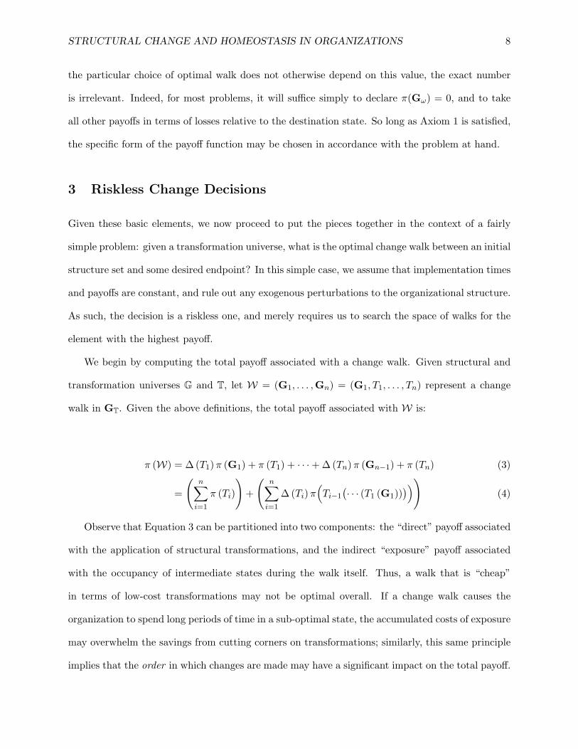
We begin by computing the total payoff associated with a change walk. Given structural and
transformation universes G and T, let W = (G1, . . . ,Gn) = (G1, T1, . . . , Tn) represent a change
walk in GT. Given the above definitions, the total payoff associated with W is:
π (W) = ∆ (T1) π (G1) + π (T1) + · · ·+ ∆ (Tn) π (Gn−1) + π (Tn) (3)
=
(n∑
i=1
π (Ti)
)+
(n∑
i=1
∆ (Ti) π(Ti−1
(· · · (T1 (G1))
)))(4)
Observe that Equation 3 can be partitioned into two components: the “direct” payoff associated
with the application of structural transformations, and the indirect “exposure” payoff associated
with the occupancy of intermediate states during the walk itself. Thus, a walk that is “cheap”
in terms of low-cost transformations may not be optimal overall. If a change walk causes the
organization to spend long periods of time in a sub-optimal state, the accumulated costs of exposure
may overwhelm the savings from cutting corners on transformations; similarly, this same principle
implies that the order in which changes are made may have a significant impact on the total payoff.

STRUCTURAL CHANGE AND HOMEOSTASIS IN ORGANIZATIONS 9
For instance, an individual can be replaced by a dismissal followed by a new hire, or by a new hire
followed by a dismissal of the original individual. In both cases, the transformations are the same,
but the optimal order will depend on the relative costs of duplicating versus being short on labor,
and on the implementation time for the hiring and dismissal processes. When labor is in short
supply, the latter procedure is preferable.
To summarize, the procedure for making an optimal riskless change decision is:
1. Define G, T, ∆, π for the problem at hand (e.g., based on empirical data, first principles,
etc.);
2. Identify the starting and ending points for the change walk, Gα and Gω;
3. Search the space of all change paths with the appropriate endpoints for a walk with the
maximum payoff;
4. Any walk with the maximum payoff is an optimal change walk, and constitutes a solution to
the change decision problem.
3.1 Properties of Optimal Change Walks
Before turning to the question of how optimal change walks may be identified, we pause momentarily
to ask whether there are any more general statements we can make about the properties of such
walks. Without knowing any further details of G, T, or π (beyond those already assumed), what
can we say about GT and W? As it happens, even these constraints are sufficient to allow for some
basic deductions regarding optimal change walks. These are interesting in and of themselves, in
addition to being useful for proving the correctness of the algorithm that follows.
Our first result concerns the “size” of the construct that is needed to solve the optimal change
walk problem. Given the tremendous multiplexity of GT – that is, the potentially large number of
edges between adjacent nodes – we are immediately led to wonder whether this profusion of ties
is really necessary. Is there a way to “throw out” superfluous ties, so as to be left with a smaller

STRUCTURAL CHANGE AND HOMEOSTASIS IN ORGANIZATIONS 10
(and in some respects, simpler) structure? The following theorem demonstrates that the answer is
affirmative:
Theorem 1. Given a payoff function π, ∀ GT ∃ a digraph HT : HT contains an optimal change
walk ∀ (Gi,Gj) having an optimal change walk in GT, which is of equal total payoff.
Proof. Given Gi,Gj ∈ G, define T ∗ (Gi,Gj) = T : T ∈ T, T (Gi) = Gj , π (T ) + ∆ (T ) π (Gi) =
maxT ′:T ′(Gi)=Gj(π (T ′) + ∆ (T ′) π (Gi)). Then let HT be a digraph whose vertex set is given by G
and whose edge set is is given by {T ∗ (Gi,Gj) : Gi,Gj ∈ G}.
We now show that all optimal change walks in GT are represented in HT. Consider two
vertices, Gα,Gω ∈ G, such that no (Gα,Gω) optimal change walk in GT belongs to HT. For
convenience, let us denote one of these walks by W∗ = (Gα, T1, . . . , Tn) = (G1, . . . ,Gn). Since
W∗ 6⊆ HT, it follows that one of two conditions holds: i) ∃ Ti ∈ W∗ : π(Ti) + ∆(Ti)π(Gi−1) <
maxT ′:T ′(Gi)=Gj(π (T ′) + ∆ (T ′) π (Gi)), or ii) π(Ti) + ∆(Ti)π(Gi−1) =
maxT ′:T ′(Gi)=Gj(π (T ′) + ∆ (T ′) π (Gi)) ∀ Ti ∈ W∗. Let us consider each in turn. If (i) is true,
then it follows that π(W∗) can be increased by selecting an alternate transformation; since this
contradicts the assumed optimality of W∗, it follows that (i) is false. If (ii) is true, then (by con-
struction) every adjacent vertex pair in is connected by an edge in HT which is of equal total value
to the corresponding edge in W∗ . This implies, however, that the total value of the corresponding
walk in HT is equal to π(W∗). Thus, this walk must be optimal, and since HT ⊆ GT, it must
also belong to GT. This contradicts our initial assumption, and thus it must be the case that all
optimal change walks in GT are represented in HT.
Intuitively, when moving between two adjacent vertices, we can effectively ignore any edges
that are not of maximum local payoff; further, since any edges that remain must be of the same
payoff, they are equally effective. Although we have focused on this result in its application to
longer walks, the logic obviously holds generically for any optimal move. Expressed as a “rule,”
the following corollary captures the key idea:

STRUCTURAL CHANGE AND HOMEOSTASIS IN ORGANIZATIONS 11
Corollary 1 (The “Local Domination” Rule). In making a one-transformation move from
Gi to Gj, it is always optimal to use a transformation with the highest immediate payoff.
Proof. By construction, every edge of HT is of maximum immediate payoff (i.e., π(T )+∆(T )π(G) =
maxT ′:T ′(Gi)=Gj(π (T ′) + ∆ (T ′) π (Gi))). By Theorem 1, HT also contains an optimal change walk
for all pairs of vertices having a change walk in GT, which is of equal total payoff to the optimal
GT walks. Thus, it follows that it is never necessary to employ a transformation that does not have
the highest immediate payoff.
Thus, as a practical matter, Corollary 1 suggests that an organization need never concern itself
with local moves which are (locally) dominated. This quickly eliminates a potentially large class
of actions from consideration. Moreover, there are other conceivable sets of actions that can be
similarly ignored in attempting to make optimal changes. One such set is the set of transformation
sequences which result in cycles, as is demonstrated by the following lemma:
Lemma 1. All optimal change walks are change paths.
Proof. Assume that there exists an optimal change walk from Gα to Gω in HT, denoted W∗, which
is not a change path. Then W∗ contains at least one cycle, C, and at least one embedded (Gα,Gω)
path, P; without loss of generality, choose P and C to be of maximum payoff. Since W∗ is optimal,
it follows that
π (P ∪ C) ≥ π(P) + ∆(C)π(Gω),
and hence that
π(C) ≥ ∆(C)π(Gω),
which, finally, implies
|{T :T∈C}|∑i=1
(π (Ti) + ∆ (Ti) π (Gi−1)) ≥|{T :T∈C}|∑
i=1
∆ (Ti) π (Gω) .
This is only possible if ∃G 6= Gω, T : π(T )+∆(T )π(G) ≥ ∆(T )π(Gω), which contradicts Axiom 1.
It therefore follows that all optimal change walks are change paths.

STRUCTURAL CHANGE AND HOMEOSTASIS IN ORGANIZATIONS 12
As before, the intuition is fairly straightforward. Given that (by Axiom 1) we would rather
be at our destination than anywhere else, actions that artificially prolong our journey cannot be
optimal. Clearly, walks that are not paths have this property, since they necessarily contain shorter
sub-walks that still reach the desired goal. This observation, like that of Theorem 1, lends itself to
a simple behavioral rule, namely:
Corollary 2 (The “No-Backsies” Rule). It is never optimal for an organization which is
changing from form Gα to Gω to revert to a previous intermediate form.
Proof. This follows immediately from Lemma 1, as any vertex sequence which contains repeated
elements cannot (by definition) constitute a path, and since optimal change walks are always
paths.
Simple as it is, the “no-backsies” rule does have some interesting implications. For instance,
it suggests that firms which are observed to “churn” personnel via repeated cycles of hiring and
firing are most likely not following an optimal change path. (Although this behavior may also be
the result of external perturbations; see below regarding this point.) In general, intendedly cyclical
behavior is diagnostic of sub-optimality. Looking for cycles may prove a useful heuristic for locating
examples of sub-optimality in the field.
3.2 Finding an Optimal Change Path
As we established with Theorem 1 and Lemma 1, the problem of finding an optimal change walk can
be reduced to that of finding a maximum payoff path on HT. This problem is simply an alternate
form of the shortest-path problem, a well-known problem of combinatorial optimization. To see
that this is so, one must merely reframe the payoff associated with the change walk in terms of
the cost of the path relative to spending the entire traversal time at the destination state. (Recall
that, by Axiom 1, the latter payoff must be strictly greater than that of any walk on GT.) Then
it follows that the path of minimum cost is that of maximum payoff, and an algorithm that solves
the former problem can also be used to solve the latter.

STRUCTURAL CHANGE AND HOMEOSTASIS IN ORGANIZATIONS 13
Although, in principle, any shortest-path algorithm could be modified to solve the optimal
change path problem (see Ahuja et al. (1993) and Cook et al. (1998) for in-depth discussions of
shortest-path algorithms) we present here a variant of Dijkstra’s well-known label-setting algorithm
(Dijkstra, 1959).6 This is shown in Algorithm 1. Although fairly typical in form, Algorithm 1 does
contain some features which relate specifically to the optimal change problem. First, and most
trivially, we exploit the fact that we are interested only in the (Gα,Gω) path by terminating
execution as soon as the shortest such path is found (see line 19). Second, as already noted, we
have reversed the usual sense of the optimization by seeking a maximum payoff path instead of
a path of minimum cost; this is operationalized by line 13, and is rendered feasible by Axiom 1.
Third, we deal with the multiplexity of GT via the loop in lines 9-18, which ensures that only
the maximum payoff (minimum cost) arc is used. Although this is presented here as a runtime
calculation in order to conserve memory, it is also in principle possible to discard all but the least
expensive edges in an initial step, thereby operating directly on HT. This seems unlikely to be
practical in most situations, but some performance gains may still be possible (depending on π and
|GT|) if some transformations could be eliminated ex ante. This leads us to our fourth significant
modification to the basic algorithm: because it will rarely if ever be feasible to store distances to all
members of G, we attempt to minimize memory usage by storing distances only for those vertices
we have visited. (Note that the default distance set by line 1 can be implemented via implicit
storage (i.e., as a default value), with explicit storage only of visited vertices.) Indeed, storage is
dominated by the distance and predecessor lists, and will be on the order of the number of vertices
visited prior to finding the shortest path. Algorithm 1 is constructed so as to minimize the number
of vertices visited, and hence should require as little storage as possible.
When executed, Algorithm 1 will yield the payoff of the optimal (Gα,Gω) path as d(Gω). The
specific path followed may be reconstructed via the predecessor list, pred, which indicates both
the predecessor and transformation employed for every visited vertex other than Gα. (One simply6The performance of Dijkstra’s algorithm is close to optimal for dense graphs (Ahuja et al., 1993), and thus it
serves as an obvious starting point for the present application.

STRUCTURAL CHANGE AND HOMEOSTASIS IN ORGANIZATIONS 14
Algorithm 1 Identification of Optimal Change Paths1: d (G) := −∞ ∀ G ∈ GT
2: d (Gα) := 0
3: vis := {Gα}
4: pred (Gα) := ∅
5: flag := False
6: while ¬flag , |vis| > 0 do
7: G := Gi ∈ vis : d (Gi) = maxGj∈vis d (Gj)
8: vis := vis \G
9: for all T ∈ T do
10: if d(T (G)
)= −∞ then
11: vis := vis ∪ T (G)
12: end if
13: δ := d (G) + π (T ) + ∆ (T )(π (G)− π (Gω)
)14: if δ > d
(T (G)
)then
15: d(T (G)
):= δ
16: pred (Gα) := (G, T )
17: end if
18: end for
19: if d (Gω) > maxGi∈vis d (Gi) then
20: flag := True
21: end if
22: end while

STRUCTURAL CHANGE AND HOMEOSTASIS IN ORGANIZATIONS 15
starts with pred(Gω) and works backwards.) If pred is stored as a tree rather than a list, this
operation can be performed linearly in the length of the optimal path. As a minor note, we have
tacitly assumed throughout this discussion that a (Gα,Gω) path actually exists; were this not
so, the optimization question would be meaningless! Still, in case the possibility of attaining an
optimal solution should be in question, a check for the size of the “to visit” stack (vis) is performed
at line 6. Should vis become empty while d(Gω) = −∞, this indicates that no (Gα,Gω) exists,
and that the optimization problem is ill-posed.
We conclude our discussion of the optimal change algorithm with a proof of its correctness:
Theorem 2. Algorithm 1 terminates with a solution to the optimal change problem, if such a
solution exists.
Proof. We begin our proof of the correctness of the algorithm by demonstrating that, at each
iteration, G is chosen so as to be “closest” (i.e., connected by a path of maximum payoff) to Gα.
(By Lemma 1, we may ignore any non-path walks.) Consider the first iteration, in which G = Gα:
by definition, Gα is closest to itself. Now, consider the nth iteration, under the assumption that all
vertices chosen so far have met the closeness condition. By step 7, the G which is chosen is closest
to Gα. Further, by the finite loop of lines 9-18, all vertices which are adjacent to G are placed at
distance d(G) plus their distance from G. Plainly, this is an upper bound on their distances (a
lower bound on the path of maximum payoff). If it is not also a lower bound for a given vertex,
then it follows from the criterion of line 7 that there exists some other vertex which will be visited
first, and which will lower the distance (raise the payoff) for said vertex (by line 14). Because every
vertex adjacent to G is added to vis, every such vertex is visited; from the forgoing, it follows that
when this vertex is visited, it will be of maximum closeness/payoff. Therefore, it follows that the
condition will be satisfied for these vertices as well, and, by induction, that the condition is satisfied
for all vertices.
Given that every vertex adjacent to a visited vertex is visited (unless the termination condition
has been met), the above implies that every vertex connected to Gα is visited in descending order of

STRUCTURAL CHANGE AND HOMEOSTASIS IN ORGANIZATIONS 16
payoff. To complete the proof, we note that the terminating conditions of lines 19 and 6 can only be
met if every other path is of strictly lower payoff than an already uncovered (Gα,Gω) path, and/or
if no vertices remain to be visited. If the latter is true, then there can exist no higher-payoff path
than that which has been uncovered (if any): if and only if π(Gω) > −∞, such a path must exist.
(Otherwise, there is no solution to find.) If the latter is false, then the observed (Gα,Gω) path is
of higher value than any other path (by the induction argument above), and we may terminate the
algorithm. The optimal change path may be derived by following the predecessors of Gω backwards
until Gα is reached.
4 Risky Change Decisions
In our discussion so far, we have avoided the vagueness and uncertainty associated with real-world
decisions: we have presumed that everything from implementation times to the payoffs associated
with particular structural forms are fixed and known. Here, we generalize our earlier results to
decisions in which implementation times and payoffs are uncertain.
Under an uncertainty assumption, implementation time and payoffs (especially the structural
payoff) are taken to be random variables rather than constants. Thus, one cannot be sure precisely
how long it will take to hire someone (for instance), or exactly what the effects will be of having lost
the manager of a particular division. Introducing such uncertainty provides for one obvious source
of risk in organizational design, and allows for decisions that are robust to unexpected delays.
For ∆, π random, the obvious optimization criterion is the expected payoff; applying the expec-
tation operator to Equation 3 gives us
E(π (W)
)= E
(∆ (T1) π (G1)
)+ E
(π (T1)
)+ · · ·
+ E(∆ (Tn) π (Gn−1)
)+ E
(π (Tn)
) (5)
=
(n∑
i=1
E(π (Ti)
))+
(n∑
i=1
E(∆ (Ti) π
(Ti−1
(· · · (T1 (G1))
))))(6)

STRUCTURAL CHANGE AND HOMEOSTASIS IN ORGANIZATIONS 17
Note that this result does not assume independence. If we are willing to take durations and
payoffs as independent, we may obtain variances in the same manner:
V ar(π (W)
)= V ar
(∆ (T1) π (G1)
)+ V ar
(π (T1)
)+ · · ·
+ V ar(∆ (Tn) π (Gn−1)
)+ V ar
(π (Tn)
) (7)
=
(n∑
i=1
V ar(π (Ti)
))+
(n∑
i=1
V ar(∆ (Ti) π
(Ti−1
(· · · (T1 (G1))
))))(8)
These may be used to assess the level of risk associated with each change path. Although we
assume risk-neutrality for the moment, the generalization of the approach to incorporate non-risk
neutral preferences is an important direction for future development.
4.1 Finding an Optimal Change Path Under Risk
Finding an optimal change path under risk is not qualitatively distinct from the riskless case. By
replacing transformation payoffs by their expectations, we may use a slightly modified version of
Algorithm 1 (using Equation 5) to identify a change path which maximizes the expected path
payoff. As before, simulation steps may need to be added to estimate expectations for payoffs
associated with structural positions, the implementation of which will obviously be problem-specific.
In general, however, the change from riskless to risky change decisions is fairly transparent in terms
of the procedures involved.
5 Structural Perturbations
The foregoing has treated the problem of optimal change decisions in an environment in which the
only source of structural change is the application of interventions by the Organizational Designer.
While we may have been uncertain regarding actual payoffs and implementation times, we were
nevertheless able to rely on the fact that the organizational structure itself was never in question.
Although reasonable as a first approximation, we are naturally led to ask how things might differ if
STRUCTURAL CHANGE AND HOMEOSTASIS IN ORGANIZATIONS 18
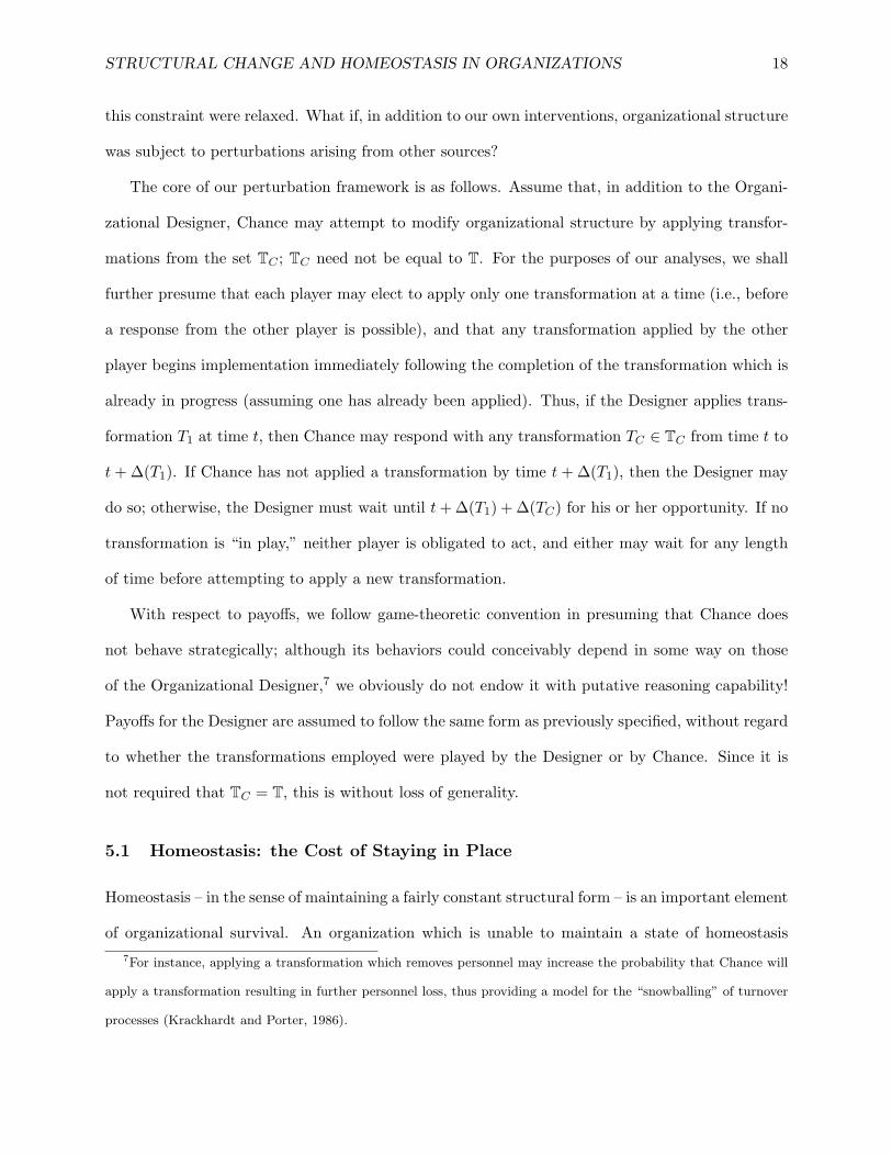
this constraint were relaxed. What if, in addition to our own interventions, organizational structure
was subject to perturbations arising from other sources?
The core of our perturbation framework is as follows. Assume that, in addition to the Organi-
zational Designer, Chance may attempt to modify organizational structure by applying transfor-
mations from the set TC ; TC need not be equal to T. For the purposes of our analyses, we shall
further presume that each player may elect to apply only one transformation at a time (i.e., before
a response from the other player is possible), and that any transformation applied by the other
player begins implementation immediately following the completion of the transformation which is
already in progress (assuming one has already been applied). Thus, if the Designer applies trans-
formation T1 at time t, then Chance may respond with any transformation TC ∈ TC from time t to
t + ∆(T1). If Chance has not applied a transformation by time t + ∆(T1), then the Designer may
do so; otherwise, the Designer must wait until t + ∆(T1) + ∆(TC) for his or her opportunity. If no
transformation is “in play,” neither player is obligated to act, and either may wait for any length
of time before attempting to apply a new transformation.
With respect to payoffs, we follow game-theoretic convention in presuming that Chance does
not behave strategically; although its behaviors could conceivably depend in some way on those
of the Organizational Designer,7 we obviously do not endow it with putative reasoning capability!
Payoffs for the Designer are assumed to follow the same form as previously specified, without regard
to whether the transformations employed were played by the Designer or by Chance. Since it is
not required that TC = T, this is without loss of generality.
5.1 Homeostasis: the Cost of Staying in Place
Homeostasis – in the sense of maintaining a fairly constant structural form – is an important element
of organizational survival. An organization which is unable to maintain a state of homeostasis7For instance, applying a transformation which removes personnel may increase the probability that Chance will
apply a transformation resulting in further personnel loss, thus providing a model for the “snowballing” of turnover
processes (Krackhardt and Porter, 1986).
STRUCTURAL CHANGE AND HOMEOSTASIS IN ORGANIZATIONS 19
for long periods of time runs the risk of incurring sufficient costs to induce mortality (Hannan
and Freeman, 1977), and simulation studies of organizations which are in constant flux suggest
that survivors may still suffer from serious degradation in performance (particularly if the rate of
change in the organizational structure overtakes the rate of change in the environment) (Carley and
Svoboda, 1996). In any event, presuming a relatively stable environment, failure of homeostasis
will almost always entail8 that an organization spend relatively large periods of time in sub-optimal
structural states, and we may thus realistically expect it to impact performance. (Indeed, studies
suggest a performance/adaptability tradeoff (Lin and Carley, 2003).)
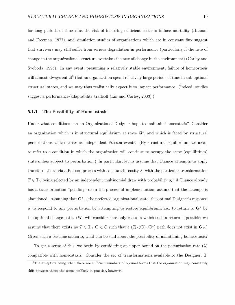
5.1.1 The Possibility of Homeostasis
Under what conditions can an Organizational Designer hope to maintain homeostasis? Consider
an organization which is in structural equilibrium at state G∗, and which is faced by structural
perturbations which arrive as independent Poisson events. (By structural equilibrium, we mean
to refer to a condition in which the organization will continue to occupy the same (equilibrium)
state unless subject to perturbation.) In particular, let us assume that Chance attempts to apply
transformations via a Poisson process with constant intensity λ, with the particular transformation
T ∈ TC being selected by an independent multinomial draw with probability pT ; if Chance already
has a transformation “pending” or in the process of implementation, assume that the attempt is
abandoned. Assuming that G∗ is the preferred organizational state, the optimal Designer’s response
is to respond to any perturbation by attempting to restore equilibrium, i.e., to return to G∗ by
the optimal change path. (We will consider here only cases in which such a return is possible; we
assume that there exists no T ∈ TC ,G ∈ G such that a(TC (G) ,G∗) path does not exist in GT.)
Given such a baseline scenario, what can be said about the possibility of maintaining homeostasis?
To get a sense of this, we begin by considering an upper bound on the perturbation rate (λ)
compatible with homeostasis. Consider the set of transformations available to the Designer, T.8The exception being when there are sufficient numbers of optimal forms that the organization may constantly
shift between them; this seems unlikely in practice, however.

STRUCTURAL CHANGE AND HOMEOSTASIS IN ORGANIZATIONS 20
Clearly, no matter what perturbation Chance applies9, the Designer cannot restore equilibrium
faster than ∆min = minT∈T ∆(T ). Thus, if λ is sufficiently large for the inter-perturbation time to
be small relative to ∆min, homeostasis becomes impossible. Given that perturbations occur as a
Poisson process, this implies the condition
1λ� ∆min (9)
or, alternately,
λ � 1∆min
. (10)
To refine this constraint somewhat, we can also consider the expected time spent in homeostasis;
that is, the expected time spent in state G∗ between perturbations. Following the above argument,
a firm lower bound on the total re-equilibration time of the organization following a perturbation is
given by ∆min. For convenience, let us refer to the inter-perturbation time as tC , with tC ∼ exp(λ).
Then a lower bound on the expected time spent in homeostasis must be given by
ε = 0p (tC ≤ ∆min) +∫ ∞
∆min
(tC −∆min
)λe−λtC dtC (11)
= −(
tC +1λ
)e−λtC
∣∣∣∣∞∆min
+ ∆mine−λtC
∣∣∣∣∞∆min
(12)
=(
0 +(
∆min +1λ
)e−λ∆min
)+(0−∆mine
−λ∆min
)(13)
=1λ
e−λ∆min . (14)
For a given bound, we can then identify the associated maximum λ by
λ ≤ 1∆min
W
(∆min
ε
), (15)
9Other than the identity transformation; since including this within TC would be equivalent to a reduction in λ,
we can safely ignore this possibility.
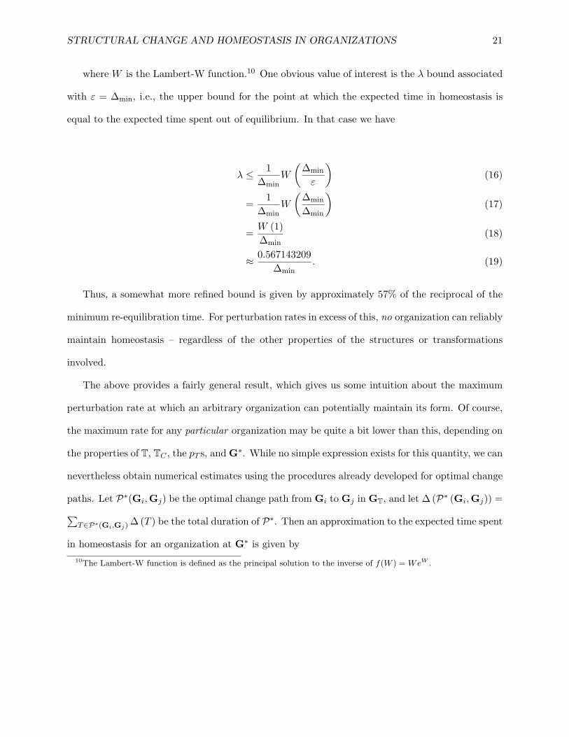
STRUCTURAL CHANGE AND HOMEOSTASIS IN ORGANIZATIONS 21
where W is the Lambert-W function.10 One obvious value of interest is the λ bound associated
with ε = ∆min, i.e., the upper bound for the point at which the expected time in homeostasis is
equal to the expected time spent out of equilibrium. In that case we have
λ ≤ 1∆min
W
(∆min
ε
)(16)
=1
∆minW
(∆min
∆min
)(17)
=W (1)∆min
(18)
≈ 0.567143209∆min
. (19)
Thus, a somewhat more refined bound is given by approximately 57% of the reciprocal of the
minimum re-equilibration time. For perturbation rates in excess of this, no organization can reliably
maintain homeostasis – regardless of the other properties of the structures or transformations
involved.
The above provides a fairly general result, which gives us some intuition about the maximum
perturbation rate at which an arbitrary organization can potentially maintain its form. Of course,
the maximum rate for any particular organization may be quite a bit lower than this, depending on
the properties of T, TC , the pT s, and G∗. While no simple expression exists for this quantity, we can
nevertheless obtain numerical estimates using the procedures already developed for optimal change
paths. Let P∗(Gi,Gj) be the optimal change path from Gi to Gj in GT, and let ∆ (P∗ (Gi,Gj)) =∑T∈P∗(Gi,Gj)
∆ (T ) be the total duration of P∗. Then an approximation to the expected time spent
in homeostasis for an organization at G∗ is given by10The Lambert-W function is defined as the principal solution to the inverse of f(W ) = WeW .

STRUCTURAL CHANGE AND HOMEOSTASIS IN ORGANIZATIONS 22
ε ≈∑
T∈TC
pT [0p (tC ≤ ∆ (P∗ (T (G∗) ,G∗)))
+∫ ∞
∆(P∗(T (G∗),G∗))(tC −∆ (P∗ (T (G∗) ,G∗)))λe−λtC
] (20)
=∑
T∈TC
pT
[−(
tC +1λ
)e−λtC
∣∣∣∣∞∆(P∗(T (G∗),G∗))
+∆ (P∗ (T (G∗) ,G∗)) e−λtC
∣∣∣∣∞∆(P∗(T (G∗),G∗))
] (21)
=∑
T∈TC
pT
[1λ
e−λ∆(P∗(T (G∗),G∗))
]. (22)
This value is an approximation of the true ε in that it does not consider any additional disrup-
tive effect of perturbations which occur during the re-equilibration process. This effect will be small
whenever∑T∈TC
pT ∆ (P∗ (T (G∗) ,G∗)) � 1λ , or (more generally) when the duration of the average per-
turbed optimal path is approximately equal to∑T∈TC
pT ∆ (P∗ (T (G∗) ,G∗)). In any event, since additional perturbations should, on average,
increase the re-equilibration time, Equation 22 serves as an upper bound on ε.
Numerical estimation is necessary to obtain the λ corresponding to ε =∑
T∈TCpT ∆ (P∗ (T (G∗) ,G∗)),
since Equation 22 cannot be solved directly. For small |TC |, this can be accomplished by using
Algorithm 1 to find the duration of each perturbed path, and then solving for λ using an iterative
search procedure (since the ∆s are independent of λ). Standard methods for such estimation can
be found in any numerical methods text, e.g. Press et al. (1986).
5.1.2 Homeostasis Costs
As we have shown, the task of maintaining homeostasis is nontrivial; indeed, if perturbations occur
with sufficient frequency, it may be difficult or impossible. Where perturbations are less frequent,
the ability of the Designer to maintain equilibrium is not in question. The cost of maintaining
equilibrium, however, is another matter. If a high-performing structural configuration is surrounded
STRUCTURAL CHANGE AND HOMEOSTASIS IN ORGANIZATIONS 23
(in the change multigraph formed by TC on G) largely by low-performing configurations, the long-
run average payoff associated with attempting to maintain this position may be severely reduced.
Here, we provide an expression for the approximate expected payoff associated with attempting
to maintain an equilibrium position, G∗. For convenience, we take all payoffs to be given relative to
π (G∗); thus, the expression can be directly interpreted as the cost associated with homeostasis. As
before, we assume Chance to apply transformations as Poisson events, with the transformation type
selected via a multinomial process. Applying these assumptions yields, for the expected homeostasis
cost per unit time,
E (π∗ (G∗)) ≈ λ∑
T∈TC
pT (π (T ) + π (P∗ (T (G∗) ,G∗))) , (23)
which converges almost surely to E (π∗ (G∗)) in the small-λ limit. (In practice, the approxi-
mation will be valid so long as∑
T∈TCpT ∆ (P∗ (T (G∗) ,G∗)) � 1
λ .) For small |TC |, Equation 23
can be calculated very straightforwardly using Algorithm 1. If |TC | is large, it may be necessary to
resort to a more restricted sampling strategy; where the distribution of transformation probabili-
ties (pT ) is extremely concentrated, one such option is to sample from TC using the transformation
probabilities. This will tend to omit low-probability transformations, while still resulting in an
unbiased estimate.
5.2 Optimal Changes Under Perturbation Risk
We have considered the question of optimal change decisions in the context of perfect information,
and under uncertainty regarding implementation time and payoffs. Finding an optimal change path
under the risk of structural perturbations is more challenging. Unlike the case of homeostasis, where
we focused on small deviations from a steady state, we now consider the effect of such perturbations
at any point along the change path. A complete solution to the optimal change problem under
perturbation risk requires a change strategy, i.e., an algorithm which provides directions on how
to proceed from each possible state towards the final objective. Such an algorithm is likely to be
infeasible for any but the very smallest organizations. Consequently a heuristic approach is called
STRUCTURAL CHANGE AND HOMEOSTASIS IN ORGANIZATIONS 24
for, with simulation used to evaluate the robustness of the various heuristic approaches.
6 Structural Changes with Multiple Decision Makers
Thus far (with the rather mindless exception of Chance), our analyses have been confined to the
decision problem faced by a single Organizational Designer who wishes to identify an optimal means
of moving ζ from Gα to Gω. One important extension of these ideas is to contexts in which multiple
decision makers are involved in the change decision; these “structural games” include strategic issues
which are absent in the “lone Designer” scenario. While there are many ways in which multiple
decision makers could enter into the change process, we focus on two: a basic principal-agent
game, and a simple bargaining problem. Although each is treated with some brevity, our aim is to
highlight basic results with reasonably broad applicability. Further investigation into the properties
of structural games is a fruitful area for further research.
6.1 Optimal Changes in a Principal-Agent Game
One of the simplest ways in which multiple decision makers can be incorporated into the present
problem is via a principal-agent framework.11 In particular, assume that associated with the
organization, ζ, there exists a Principal, whose payoffs are given by πP , and a set of Agents, A,
each with individual payoff function πa and transformation universe Ta. It is assumed that (under
conditions of perfect information) the Principal wishes to take ζ from Gα to Gω, but is unable to
do so directly. The problem facing the Principal, then, is to select the Agent (would-be Designer)
whose solution to the optimal change path problem is most highly valued.
To solve this problem, we begin by denoting by P∗πT (Gα,Gω) the optimal change path from Gα
to Gω in the change multigraph GT under payoff function π. Then, the solution for the Principal
is to find an agent a ∈ A such that one of the following is satisfied:11We are indebted to David Rode for this suggestion.

STRUCTURAL CHANGE AND HOMEOSTASIS IN ORGANIZATIONS 25
πP
(P∗
πaTa(Gα,Gω)
)= max
a′∈AπP
(P∗
πa′Ta′(Gα,Gω)
)(24)
πP
(P∗
πTa(Gα,Gω)
)= max
a′∈AπP
(P∗
πTa′(Gα,Gω)
)(25)
πP
(P∗
πaT (Gα,Gω))
= maxa′∈A
πP
(P∗
πa′T (Gα,Gω))
(26)
Each of these criteria corresponds to the subgame-perfect Nash equilibrium for a different
potential game.12 Equation 24 reflects a game with unenforceable commitments and differing
individual capabilities. That is, the Principal cannot enforce his or her preferences on the Agent
(who, it is assumed, will maximize his or her own payoffs), and each Agent has a potentially unique
set of transformations which may be applied to the optimal change problem.13 In this case, then,
the Principal examines the solutions which each agent is anticipated to produce, and selects an
agent whose solution produces the highest payoff under πP .
The second criterion, Equation 25, provides the strategy for a game with enforceable commit-
ments and differing individual capabilities. Here, it is assumed, the Principal can credibly enforce
his or her own preferences vis a vis the Agent; for simplicity, we assume here that this enforcement
is perfect, and thus that each Agent acts as if he or she had preference function πP . While each
Agent will then attempt to maximize πP , the fact that each possesses a distinct transformation
universe means that not every Agent will necessarily be successful in the attempt. As before, the
Principal selects an Agent whose anticipated solution maximizes πP .
Finally, Equation 26 gives the equilibrium strategy for a Principal-Agent game in which the
Principal’s preferences are unenforceable, but in which all Agents have the same capabilities. Here,
while each Agent has the same ability to match πP , each may differ on the extent that they prefer
to do so. Given this, the Principal selects an Agent whose personally optimal solution he or she
most values.12We omit the case in which commitments are enforceable and all Agents have the same capabilities, since this is
merely the standard optimal change problem.13We further assume that the Principal’s preferences over all such potential transformations are well-formed.
STRUCTURAL CHANGE AND HOMEOSTASIS IN ORGANIZATIONS 26
With respect to all of the above, it should be noted that actual solutions to the Principal-Agent
change game for particular parameter choices can be obtained straightforwardly via a combination
of the appropriate strategy (Equations 24-26) and the solutions generated by Algorithm 1. In cases
where a solution to the optimal path problem does not exist for one or more Agents, this should
be treated as a distinct outcome and evaluated accordingly (i.e., this should be given a payoff in
πP ). Note, since some agents may not prefer Gω to all other states, it is not unreasonable that
such defections will occur without enforcement! Thus, this approach manages to implicitly include
enforcement problems related to disagreements regarding goals, as well as those that relate strictly
to plans of implementation.
6.2 Pareto-Optimal Change Walks
A second simple scenario involving multiple decision makers arises from a situation in which the
(ostensibly singular) Organizational Designer is actually a committee. If multiple individuals with
divergent payoffs set out to plan an organizational change, what can we say regarding their eventual
solution? Without delving too deeply into the context of the bargaining game played by these actors,
we can still place some bounds on their decision by noting that any change walk they select must
be Pareto-optimal. In terms of the present problem, Pareto-optimality is defined as follows:
Definition 6. Given a set of actors, A, each with payoff function πa and common transformation
universe T, let W (Gα,Gω) be the set of all (Gα,Gω) walks in GT. Then, for two walks Wi,Wj ∈
W (Gα,Gω),Wi is said to (strongly) Pareto-dominateWj (denotedWiBWj) iff ∃ a ∈ A : πa (Wi) >
πa (Wj) and @ b ∈ A : πb (Wi) < πb (Wj). A walk W ∈ W (Gα,Gω) is said to be Pareto-optimal iff
@ Wi ∈ W (Gα,Gω) : Wi BW.
Thus, any change walk that is Pareto-dominated will not be selected, since there is at least one
actor who would benefit from an alternative, and none who would suffer. Given this, which walks
are Pareto-optimal? While this is difficult to determine in the general case, we can identify some
Pareto-optimal walks that are particularly salient. Optimal change paths, for instance, are likely

STRUCTURAL CHANGE AND HOMEOSTASIS IN ORGANIZATIONS 27
candidates, as is demonstrated by the following theorem:
Theorem 3. Let P∗πa(Gα,Gω) ⊆ GT be the set of optimal change paths for some actor a ∈ A.
Then ∃ P∗ ∈ P∗πa(Gα,Gω) : P∗ is Pareto-optimal.
Proof. Assume that @ P∗ ∈ P∗πa(Gα,Gω) : P∗ is Pareto-optimal. Then it follows that ∃ W ∈
W (Gα,Gω) : W B P∗ ∀ P∗ ∈ P∗πa(Gα,Gω). Further, we know that W 6∈ P∗πa
(Gα,Gω), since
otherwise P∗πa(Gα,Gω) would have a Pareto-optimal member. However, if W 6∈ P∗πa
(Gα,Gω),
then by definition πa (W) < πa (P∗) ∀ P∗ ∈ P∗πa(Gα,Gω), and hence W cannot Pareto-dominate
any member of P∗πa(Gα,Gω). This contradicts our initial assumption, and hence P∗πa
(Gα,Gω)
must contain some P∗ which is Pareto-optimal.
A trivial corollary of Theorem 3 is that unique optimal change paths are necessarily Pareto-
optimal. Another obvious implication of this result is a simple procedure for finding Pareto-optimal
walks: we pick an actor, find P∗πa(Gα,Gω) using standard methods, and check each member against
the others until we find one which is not dominated. Since the set of optimal change paths is likely
to be small, the computational burden of this procedure will not be appreciably greater than the
optimal path problem. While this does not generate the full set of Pareto-optimal walks, it does
identify certain key candidates. Since these paths also have the property of being optimal for at
least one actor, we assume that they will be of particular interest to the Organizational Designers.
7 Conclusion
As we have shown, a decision-theoretic approach to the problem of structural change in organiza-
tions offers a number of potentially useful insights for the theory of organizations. Normatively,
this perspective has allowed us to identify optimal change paths for organizations under a range of
assumptions (including uncertainty in implementation times and/or payoffs), to compute relative
expected costs for the maintenance of homeostasis under external perturbations, to solve simple
principal-agent problems involving the selection of Designers, and to find Pareto-optimal change

STRUCTURAL CHANGE AND HOMEOSTASIS IN ORGANIZATIONS 28
paths for scenarios involving multiple decision makers with conflicting interests. Descriptively, we
have been able to demonstrate minimal conditions for structural homeostasis in organizations, and
to provide bounds on the expected time spent in equilibrium for various perturbation regimes. More
importantly, by supplying a normative model for organizational change, we have also provided a
descriptive baseline from which to assess the change behavior of real organizations.
While our theorizing has covered a fair amount of ground, there are numerous important di-
rections left unconsidered. We have, for instance, given somewhat short shrift to the problem of
decisions under uncertainty for Designers who are not risk neutral; this is certainly an issue which
should be considered more deeply in future work. Another important assumption whose relaxation
is of great interest is that of destination certainty. While we have quite explicitly presumed framed
our analysis in terms of a well-defined change problem, it seems probable that, in many situations,
the Designer will not be certain as to which destination is optimal. The identification of paths that
are optimal under destination uncertainty is then complicated by the need to value the embed-
ded options associated with each path (i.e., the payoff associated with the opportunity to change
destination during the change process). This is a worthy topic for further development.
We recognize that theory alone can only take us so far. Measurement of structural and trans-
formation payoffs, techniques for the identification of minimal transformation universes, and the
like are essential for the practical application of these techniques. Nevertheless, by providing a
formal decision-theoretic framework in which the problem of organizational change and redesign
can be analyzed, we have created a framework that advances both organizational science and orga-
nizational engineering. This framework moves the discussion from the basic question “when should
organizations seek to adapt?”, to the more nuanced question, “how should organizations seek to
adapt?” It also raises the question of when and how organizations can resist pressure to change,
an often-overlooked issue in organizational evolution. In a turbulent world, it may be all one can
do to simply stay in place.
STRUCTURAL CHANGE AND HOMEOSTASIS IN ORGANIZATIONS 29
8 References
Ahuja, R. K., Magnanti, T. L., and Orlin, J. B. (1993). Network Flows: Theory, Algorithms, and
Applications. Prentice-Hall, Upper Saddle River, NJ.
Arrow, K. J. (1974). The Limits of Organization. W.W. Norton, New York.
Baligh, H., Burton, R. M., and Obel, B. (1990). Devising expert systems in organization theory:
The Organizational Consultant. In Masuch, M., editor, Organization, Management, and Expert
Systems, pages 35–57. Walter de Gruyter, Berlin.
Blau, P. M. (1972). Interdependence and hierarchy in organizations. Social Science Research,
1:1–24.
Burton, R. M. and Obel, B. (1984). Designing Efficient Organizations: Modelling and Experimen-
tation. North Holland, Amsterdam.
Carley, K. M. (2002a). Computational organizational science and organizational engineering. Sim-
ulation Modeling Practice and Theory, 10:253–269.
Carley, K. M. (2002b). Smart agents and organizations of the future. In Lievrouw, L. and Living-
stone, S., editors, The Handbook of New Media, pages 206–220. Sage, Thousand Oaks, CA.
Carley, K. M., Dombroski, M., Tsvetovat, M., Reminga, J., and Kamneva, N. (2003). Destabilizing
dynamic covert networks. In Proceedings of the 8th International Command and Control Research
and Technology Symposium, National Defense War College, Washington DC. Evidence Based
Research.
Carley, K. M. and Hill, V. (2001). Structural change and learning within organizations. In Lomi,
A. and Larsen, E. R., editors, Dynamics of Organizations: Computational Modeling and Orga-
nizational Theories, chapter 2, pages 62–92. MIT Press, Cambridge, MA.

STRUCTURAL CHANGE AND HOMEOSTASIS IN ORGANIZATIONS 30
Carley, K. M. and Krackhardt, D. (1998). A PCANS model of structure in organization. In Proceed-
ings of the 1998 International Symposium on Command and Control Research and Technology,
Monterray, CA.
Carley, K. M. and Krackhardt, D. (1999). A typology for C2 measures. In Proceedings of the 1999
International Symposium on Command and Control Research and Technology, Newport, RI.
Carley, K. M. and Svoboda, D. M. (1996). Modeling organizational adaptation as a simulated
annealing process. Sociological Methods and Research, 25(1):138–168.
Cook, W. J., Cunningham, W. H., Pulleyblank, W. R., and Schrijver, A. (1998). Combinatorial
Optimization. John Wiley and Sons, New York.
Crowston, K. (1994). Evolving novel organizational forms. In Carley, K. M. and Prietula, M. J.,
editors, Computational Organizational Theory, pages 19–38. Lawrence Erlbaum Associates, Hills-
dale, NJ.
Dawes, R. M. (1996). Behavioral decision making and judgment. In Gilbert, D., Fiske, S., and
Lindzey, G., editors, The Handbook of Social Psychology. McGraw-Hill, Boston, MA.
Dijkstra, E. (1959). A note on two problems in connexion with graphs. Numeriche Mathematics,
1:269–271.
Duncan, R. B. (1979). What is the right organizational form? Organizational Dynamics, Winter,
1979:59–79.
Galbraith, J. (1977). Organizational Design. Addison-Wesley, Reading, MA.
Glance, N. S. and Huberman, B. A. (1994). Social dilemmas and fluid organizations. In Car-
ley, K. M. and Prietula, M. J., editors, Computational Organizational Theory, pages 217–239.
Lawrence Erlbaum Associates, Hillsdale, NJ.
Hannan, M. T. and Freeman, J. (1977). The population ecology of organizations. American Journal
of Sociology, 82(5):929–964.

STRUCTURAL CHANGE AND HOMEOSTASIS IN ORGANIZATIONS 31
Krackhardt, D. and Porter, L. W. (1986). The snowball effect: Turnover embedded in communi-
cation networks. Journal of Applied Psychology, 71(1):50–55.
Levchuk, G. M., Levchuk, Y. N., Luo, J., Pattipati, K. R., and Kleinman, D. L. (2002a). Normative
Design of Organizations - Part I: Mission Planning. IEEE Transactions on Systems, Man, and
Cybernetics: Part A - Systems and Humans, 32(3):346–359.
Levchuk, G. M., Levchuk, Y. N., Luo, J., Pattipati, K. R., and Kleinman, D. L. (2002b). Normative
Design of Organizations - Part II: Organizational Structures. IEEE Transactions on Systems,
Man, and Cybernetics: Part A - Systems and Humans, 32(3):360–375.
Levchuk, G. M., Meirina, C., Pattipati, K. R., and Kleinman, D. L. (2004). Normative Design of
Project-Based Organizations - Part III: Modeling Congruent, Robust, and Adaptive Organiza-
tions. IEEE Transactions on Systems, Man, and Cybernetics: Part A - Systems and Humans,
34(3):337–350.
Levchuk, Y., Levchuk, J., Luo, F. T., and Pattipati, K. (2000). Optimization algorithms for
organizational design. In IEEE International Conference on Systems, Man and Cybernetics,
Nashville, TN.
Levitt, R. E., Cohen, G. P., Kunz, J. C., Nass, C. I., Christiansen, T., and Jin, Y. (1994). The
“Virtual Design Team”: Simulating how organization structure and information processing tools
affect team performance. In Carley, K. M. and Prietula, M. J., editors, Computational Organi-
zational Theory, pages 1–18. Lawrence Erlbaum Associates, Hillsdale, NJ.
Lin, Z. (1994). A theoretical evaluation of measures of organizational design: Interrelationship
and performance predictability. In Carley, K. M. and Prietula, M. J., editors, Computational
Organizational Theory, pages 113–159. Lawrence Erlbaum Associates, Hillsdale, NJ.
Lin, Z. and Carley, K. M. (2003). Designing Stress Resistant Organizations: Computational Theo-
rizing and Crisis Applications. Kluwer, Boston, MA.
STRUCTURAL CHANGE AND HOMEOSTASIS IN ORGANIZATIONS 32
Lincoln, J. R., Hanada, M., and McBride, K. (1986). Organizational structures in Japanese and
U.S. manufacturing. Administrative Science Quarterly, 31:338–364.
Mackenzie, K. D. (1978). Organizational Structures. AHM, Arlington Heights, IL.
Perdu, D. M. and Levis, A. H. (1998). Adaptation as a morphing process: A methodology for the
design and evaluation of adaptive organizational structures. Computational and Mathematical
Organization Theory, 4(1):5–41.
Perrow, C. (1970). Organizational Analysis: A Sociological View. Wadsworth, Belmont, CA.
Pfeffer, J. and Salancik, G. R. (1978). External Control of Organizations. Harper and Row, New
York.
Press, W. H., Flannery, B. P., Teukolsky, S. A., and Vetterling, W. T. (1986). Numerical Recipes:
The Art of Scientific Computing. Cambridge University Press, Cambridge.
Thompson, J. D. (1967). Organizations in Action: Social Science Bases of Administrative Theory.
McGraw Hill, New York.
Tversky, A. and Kahneman, D. (1986). Rational choice and the framing of decisions. Journal of
Business, 59(4–2):S251–S278.
Williamson, O. (1975). Markets and Hierarchies, Analysis and Antitrust Implications: A Study in
the Economics of Internal Organizations. Free Press, New York.