Lecture Note on Strong Motion Seismology

Kojiro Irikura (Aichi Institute of Technology and Kyoto University) Hiroe Miyake (Earthquake Research Institute, University of Tokyo)

Chapter 1. Preface Chapter 2. Empirical Green’s Function Method Chapter 3. Theoretical Simulation (3D FDM) Chapter 4. Hybrid Method Chapter 5. Recipe for Predicting Strong Ground Motion

2

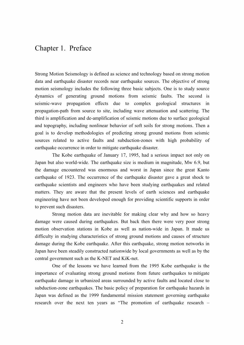
Chapter 1. Preface

Strong Motion Seismology is defined as science and technology based on strong motion data and earthquake disaster records near earthquake sources. The objective of strong motion seismology includes the following three basic subjects. One is to study source dynamics of generating ground motions from seismic faults. The second is seismic-wave propagation effects due to complex geological structures in propagation-path from source to site, including wave attenuation and scattering. The third is amplification and de-amplification of seismic motions due to surface geological and topography, including nonlinear behavior of soft soils for strong motions. Then a goal is to develop methodologies of predicting strong ground motions from seismic sources related to active faults and subduction-zones with high probability of earthquake occurrence in order to mitigate earthquake disaster.

The Kobe earthquake of January 17, 1995, had a serious impact not only on Japan but also world-wide. The earthquake size is medium in magnitude, Mw 6.9, but the damage encountered was enormous and worst in Japan since the great Kanto earthquake of 1923. The occurrence of the earthquake disaster gave a great shock to earthquake scientists and engineers who have been studying earthquakes and related matters. They are aware that the present levels of earth sciences and earthquake engineering have not been developed enough for providing scientific supports in order to prevent such disasters.

Strong motion data are inevitable for making clear why and how so heavy damage were caused during earthquakes. But back then there were very poor strong motion observation stations in Kobe as well as nation-wide in Japan. It made us difficulty in studying characteristics of strong ground motions and causes of structure damage during the Kobe earthquake. After this earthquake, strong motion networks in Japan have been steadily constructed nationwide by local governments as well as by the central government such as the K-NET and KiK-net.

One of the lessons we have learned from the 1995 Kobe earthquake is the importance of evaluating strong ground motions from future earthquakes to mitigate earthquake damage in urbanized areas surrounded by active faults and located close to subduction-zone earthquakes. The basic policy of preparation for earthquake hazards in Japan was defined as the 1999 fundamental mission statement governing earthquake research over the next ten years as “The promotion of earthquake research –

3

comprehensive basic policies for the promotion of seismic research through the observation, measurement, and survey of earthquakes –“, established by the Headquarters for Earthquake Research Promotion (Director: Ministry of Education, Culture, Sports, Science, and Technology). It proposed developments of making seismic hazard maps by promoting the survey of active faults, long-term evaluation of occurrence potentials and prediction of strong ground motion.

The Earthquake Research Committee under the Headquarter started to make the seismic hazard maps from two different approaches, probabilistic and deterministic. The probabilistic seismic hazard map is shown as the predicted likelihood of a ground motion level such as PGA, PGV, and seismic intensity occurring in a given area within a set period of time. It provides important information for land planning, design standards of structures and people’s enlightening as to seismic risks. The deterministic seismic hazard map is shown as the distribution of the ground motion level predicted for a specific earthquake fault. The strong ground motions at specific sites near the source fault should be estimated as time histories as well as shaking levels. The ground motion time histries are effectively used for nonlinear dynamic analysis of structures, which are needed to design earthquake-resistant buildings, bridges, lifelines, and so on, in particular to secure seismic safety of critical structures such as and nuclear power plants.

To obtain the ground motion time histories (waveforms) from individual specific earthquakes, we have developed a new methodology, “recipe of strong motion prediction”. This recipe give source modeling for specific earthquakes based on source characteristics from the waveform inversion using strong motion data. Main features of the source models are characterized by three kinds of parameters, which we call: outer, inner, and extra fault parameters. The outer fault parameters are to outline the overall pictures of the target earthquakes such as entire source area and seismic moment. The inner fault parameters are parameters characterizing stress heterogeneity inside the fault area. The extra fault parameters are considered to complete the source model such as the starting point and propagation pattern of the rupture. The validity and applicability of the procedures for characterizing the earthquake sources for strong ground prediction are examined in comparison with the observed records and broad-band simulated motions for recent earthquakes such as the 1995 Kobe and the 2003 Tokachi-Oki earthquakes. In future directions, prediction of strong ground motions are encouraged to constrain fault parameters physically taking into account the source dynamics as well as empirically from past earthquakes.

After the 1995 Kobe earthquake, disastrous earthquakes have still happened

4

killing about 17,000 people in 1999 Kocaeli, Turkey, about 22,300 people in Gujarato, India, 31,000 in Bam, India, and so on. Further, very recently the 2004 Ache earthquake occurring north-west off the Sumatra Island generated catastrophic tsunamis that hit coastal areas in the Indian Ocean as well as Indonesia where more than 200,000 people were killed. The 2005 Kashmir earthquake occurring in northern Pakistan flattened almost all houses and structures due to strong shaking in towns near the source areas, killing more than 80,000 people. There were very few seismometers for observing strong ground motions stations during those earthquakes. It is not easy to make clear what were near-field ground motions bringing to destruction of houses and structures if not any records. Another point is that seimometers for warning tsunami are distributed biasedly in the Pacific Ocean but few in the Indian Ocean.

These facts again taught us the importance of strong motion prediction and seismic hazard analysis as well as warning systems for tsunami to mitigate earthquake disasters.

Kojiro Irikura

5

Chapter 2. Empirical Green’s Function Method

Introduction

One of the most effective methods for simulating broadband strong ground motion that comes from a large earthquake is to use observed records from small earthquakes occurring around the source area of a large earthquake. Actual geological structure from source to site is generally more complex than that assumed in theoretical models. So actual ground motion is complicated not only by refraction and reflection due to layer interfaces and ground surface but also by scattering and attenuation due to lateral heterogeneities and anelastic properties in the propagation path. Complete modeling of the wave field in realistic media would be extremely difficult. A semi-empirical approach attempts to overcome such difficulties. In this chapter, we describe the basic theory in simulating strong ground motion for a large earthquake, incorporating the similarity law of earthquakes in the formulation. Then several applications to the source modeling and ground motion simulation using the empirical Green’s function method applications to several earthquakes are described. Formulation of the Empirical Green’s Function Method

The technique by which waveforms for large events are synthesized follows the empirical Green's function method proposed by Hartzell (1978). Revisions have been made by Kanamori (1979), Irikura (1983, 1986), and others. We introduce the empirical Green's function method formulated by Irikura (1986), based on a scaling law of fault parameters for large and small events (Kanamori and Anderson, 1975) and the omega-squared source spectra (Aki, 1967). The waveform for a large event is synthesized by summing the records of small events with corrections for the difference in the slip velocity time function between the large and small events following the above scaling laws. This method does not require knowledge of the explicit shape of the slip velocity time function for the small event.

The numerical equations to summing records of small events are,

U(t) =rrij

F(t)∗ j=1

N

∑i=1

N

∑ (C ⋅ u(t)) (1)

F(t) = δ(t − tij ) +1n '

[δk =1

(N−1)n'

∑ {t − tij −(k −1)T(N −1)n'

}] (2)

6

tij =rij − ro

Vs

+ξ ij

Vr

(3)

where, U(t) is the simulated waveform for the large event, u(t) the observed waveform for the small event, N and C are the ratios of the fault dimensions and stress drops between the large and small events, respectively, and the * indicates convolution. F(t) is the filtering function (correction function) to adjust the difference in the slip velocity time functions between the large and small events. Vs and Vr are the S-wave velocity near the source area and the rupture velocity on the fault plane, respectively. T is the risetime for the large event, and defined as duration of the filtering function F(t) (in Fig. 1(b) and (c)). It corresponds the duration of slip velocity time function on subfault from the beginning to the time before the tail starts. n’ is an appropriate integer to weaken artificial periodicity of n, and to adjust the interval of the tick to be the sampling rate. The other parameters are given in Fig 1(a).

Regarding the filtering function F(t), Irikura et al. (1997) proposed a modification to equation (2) in order to prevent sag at multiples of 1/T (Hz) from appearing in the amplitude spectra. The discretized equation for the modified F(t) is,

F( t) = δ(t − tij )+1

n '(1−1e

)[

1

e(k −1)

(N −1)n '

δk =1

(N −1)n '

∑ {t − tij −(k −1)T(N −1)n '

}] (4)

The shape of equation (4) is shown in Fig. 1(c). In Irikura (1986), the scaling parameters needed for this technique, N (integer value) and C, can be derived from the constant levels of the displacement and acceleration amplitude spectra of the large and small events with the formulas,

Uo

uo

=Mo

mo

= CN 3 (5)

Ao

ao

= CN (6)

Here, U0 and u0 indicate the constant levels of amplitude of the displacement spectra for the large and small events, respectively. M0 and m0 correspond to the seismic moments for the large and small events. A0 and a0 indicate the constant levels of the amplitude of the acceleration spectra for the large and small events (Fig. 1(d), (e)).

N and C are derived from equations (5) and (6),

7

N =U0

u0

⎛

⎝ ⎜ ⎜

⎞

⎠ ⎟ ⎟

12 a0

A0

⎛

⎝ ⎜ ⎜

⎞

⎠ ⎟ ⎟

12 (7)

C =u0

U0

⎛

⎝ ⎜ ⎜

⎞

⎠ ⎟ ⎟

12 A0

a0

⎛

⎝ ⎜ ⎜

⎞

⎠ ⎟ ⎟

32 (8)

Figure 1. Schematic illustrations of the empirical Green's function method. (a) Fault areas of large and small events are defined to be L×W and l×w, respectively, where L/l = W/w = N. (b) Filtering function F(t) (after Irikura, 1986) to adjust to the difference in slip velocity function between the large and small events. This function is expressed as the sum of a delta and a boxcar function. (c) Modified filtering function (after Irikura et al., 1997) with an exponentially decaying function instead of a boxcar function. T is the risetime for the large event. (d) Schematic displacement amplitude spectra following the omega-squared source scaling model, assuming a stress drop ratio C between the large and small events. (e) Acceleration amplitude spectra following the omega-squared source scaling model.

8

Figure 2. The effect of correction function F(t) used in the empirical Green’s function method on the

synthetic slip velocity. The slip velocity of element event is a function of Kostrov-type with a finite slip duration (left). The correction function F(t) is (a) boxcar considering only low-frequency scaling by Irikura (1983), (b) conventional one (delta + boxcar functions) by Irikura (1986), (c) modified one (delta + exponential-decay functions) by Irikura et al. (1997). And (d) normalized Kostrov-type function with a finite slip duration given by Day (1982). The spectral shapes of correction functions F(t) are shown in the right.

Parameter Estimation for the Empirical Green's Function Method by the Source Spectral Fitting Method

For an objective estimation of parameters N and C, which are required for the empirical Green’s function method of Irikura (1986), Miyake et al. (1999) proposed a source spectral fitting method. This method derives these parameters by fitting the

9

observed source spectral ratio between the large and small events to the theoretical source spectral ratio, which obeys the omega-squared source model of Brune (1970, 1971).

The observed waveform O(t) can be expressed as a convolution of the source effect S(t), propagation path effect P(t), and site amplification effect G(t) assuming linear systems; O( t) = S( t)∗ P(t) ∗G(t) (9)

In the frequency domain, the observed spectrum O(f) is expressed as a product of these effects; O( f ) = S( f ) ⋅ P( f ) ⋅G( f ) (10)

From equation (10), the observed source amplitude spectral ratio of the large and small events for one station is,

S( f )s( f )

=O( f ) P( f )o( f ) p( f )

=O( f ) 1

Re

− πfRQs ( f )Vs

o( f ) 1r

e−πfr

Qs ( f )Vs

(11)

, where capital and lowercase letters indicate the factors for the large and small events, respectively. The propagation path effect is given by geometrical spreading for the body waves and by a frequency-dependent attenuation factor Qs(f) for the S-waves.

The observed source amplitude spectral ratio for each station is first calculated using the mainshock and its aftershock. Then the observed source amplitude spectral ratio is divided into m windows in the frequency domain, in which the central frequency is fi (i=1 to m), and the log-averages S(fi)/s(fi) and the log standard deviations S.D.(fi) were obtained (Fig. 4).

The equation for the amplitude spectra, based on the omega-squared source model by Brune (1970, 1971) is given as,

S( f ) =M0

1+ f fc( )2 (12)

where, fc is the corner frequency. Using equation (12), the source spectral ratio function (SSRF) is,

SSRF( f ) =M0

m0

⋅1 + f fca( )2

1 + f fcm( )2 (13)

M0/m0 indicates the seismic moment ratio between a large and small event at the lowest frequency, and fcm and fca respectively are corner frequencies for the mainshock and aftershock. We searched the minimum value of the weighted least-squares (equation

10

(14)), applying to the observed source amplitude spectral ratio, equation (11), to fit the SSRF (equation (13), Fig. 4) in the frequency domain for nst stations;

SSRF ( fi) − S( fi) s( fi)S .D.( fi)

⎛

⎝ ⎜ ⎜

⎞

⎠ ⎟ ⎟

i=1

nst

∑2

= min (14)

This method provides estimates of M0/m0, fcm, and fca. The relationships between these parameters, N, and C are given as, Mo

mo

= CN 3 ( f → 0) (15)

Mo

mo

⎛

⎝ ⎜ ⎜

⎞

⎠ ⎟ ⎟

fcm

fca

⎛

⎝ ⎜ ⎜

⎞

⎠ ⎟ ⎟

2

= CN ( f → ∞) (16)

The high-frequency limit )( ∞→f corresponds to the frequency where the acceleration source spectrum is constant at frequencies of more than fca and less than fmax (fmax is the high-frequency cut-off of the constant level of acceleration source spectrum). According to equations (15) and (16), N and C are,

N =fca

fcm

(17)

C =Mo

mo

⎛

⎝ ⎜ ⎜

⎞

⎠ ⎟ ⎟

fcm

fca

⎛

⎝ ⎜ ⎜

⎞

⎠ ⎟ ⎟

3

(18)

11

Figure. 3. Map showing the dataset used for the 1997 Kagoshima-ken Hokuseibu earthquake of

March 26, 1997 (MJ6.5) and aftershock distributions.

Figure 4. Source spectral ratios of the mainshock to aftershock records used as the empirical Green's

function for the 1997 Kagoshima-ken Hokuseibu earthquake, March. Left: Spectral ratios for all the sites. Right: Comparison of average values of the observed ratios and best-fit source spectral ratio function (SSRF, broken line). Closed circles represent the average, bars the standard deviation of the observed ratios.

12

Near-Source Ground Motion Simulation to Estimate Strong Motion Generation Area

The modeling of the strong motion generation area using the empirical Green’s function method is one of the useful means to kinematically simulate both low- and high-frequency wave generations from the source using appropriate filtering function F(t). The filtering function F(t) provide the rupture growth with Kostrov-like slip velocity time functions.

We define the “strong motion generation area” as the area characterized by a large uniform slip velocity within the total rupture area, which reproduces near-source strong ground motions up to 10 Hz. The strong motion generation area of each mainshock is estimated by waveform fitting based on the empirical Green's function method. The low-frequency limit is constrained by the signal to noise level ratio of the small event record used as an empirical Green's function.

There are lots of studies to perform ground motion simulations of the target earthquakes using the empirical Green’s function method in order to estimate the strong motion generation area. These simulations utilized acceleration, velocity, and displacement records from several stations surrounding the source area. The frequency range available for simulation was generally from 0.2 to 10 Hz, depending on the noise levels of the aftershock records. The S-wave arrival times of the velocity waveforms for the target and element earthquakes first were set, then 5 parameters, representing the size (length and width) and position (starting point of the rupture in the strike and dip directions) for the strong motion generation area, and risetime, were estimated to minimize the residuals of the displacement waveform and acceleration envelope fitting. The fitting was done by the Genetic Algorithm method (e.g., Holland, 1975) or forward modeling.

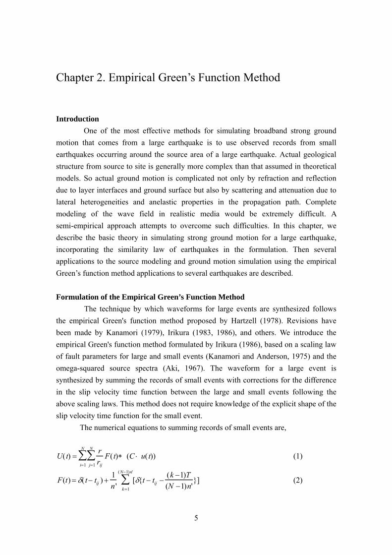
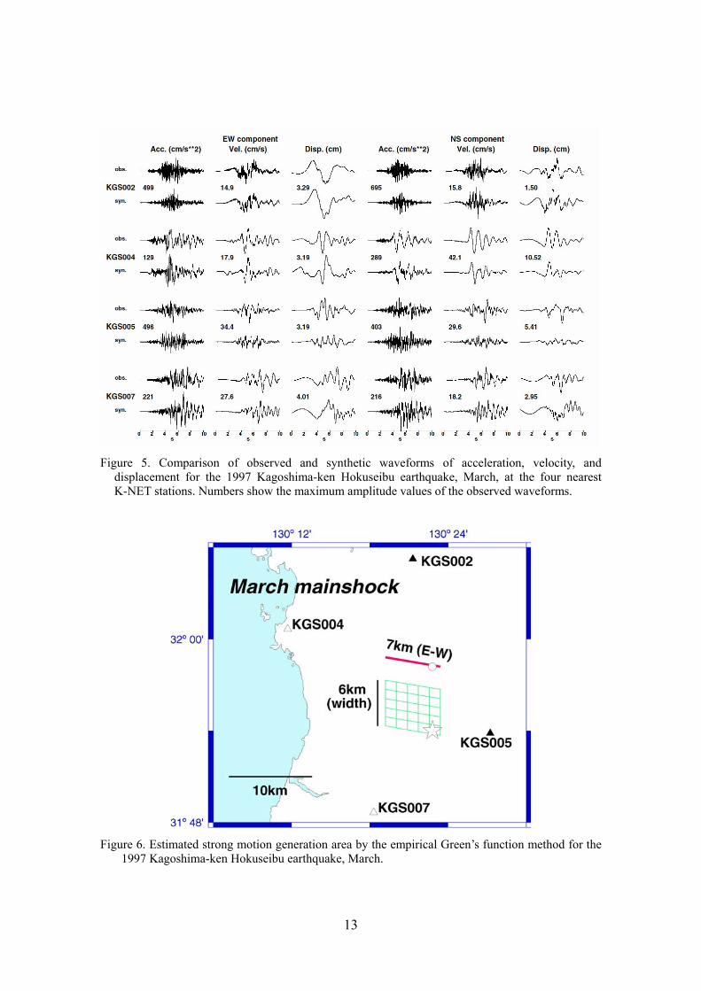
Following this approach, we estimate the strong motion generation areas, for the target earthquakes. Synthetic waveforms for the best source models fit the observed data well in the acceleration and velocity, while some displacement synthetics seem to be smaller amplitude than the observations (Fig. 5). The estimated strong motion generation area is shown in Fig. 6.

13

Figure 5. Comparison of observed and synthetic waveforms of acceleration, velocity, and

displacement for the 1997 Kagoshima-ken Hokuseibu earthquake, March, at the four nearest K-NET stations. Numbers show the maximum amplitude values of the observed waveforms.

Figure 6. Estimated strong motion generation area by the empirical Green’s function method for the

1997 Kagoshima-ken Hokuseibu earthquake, March.

14

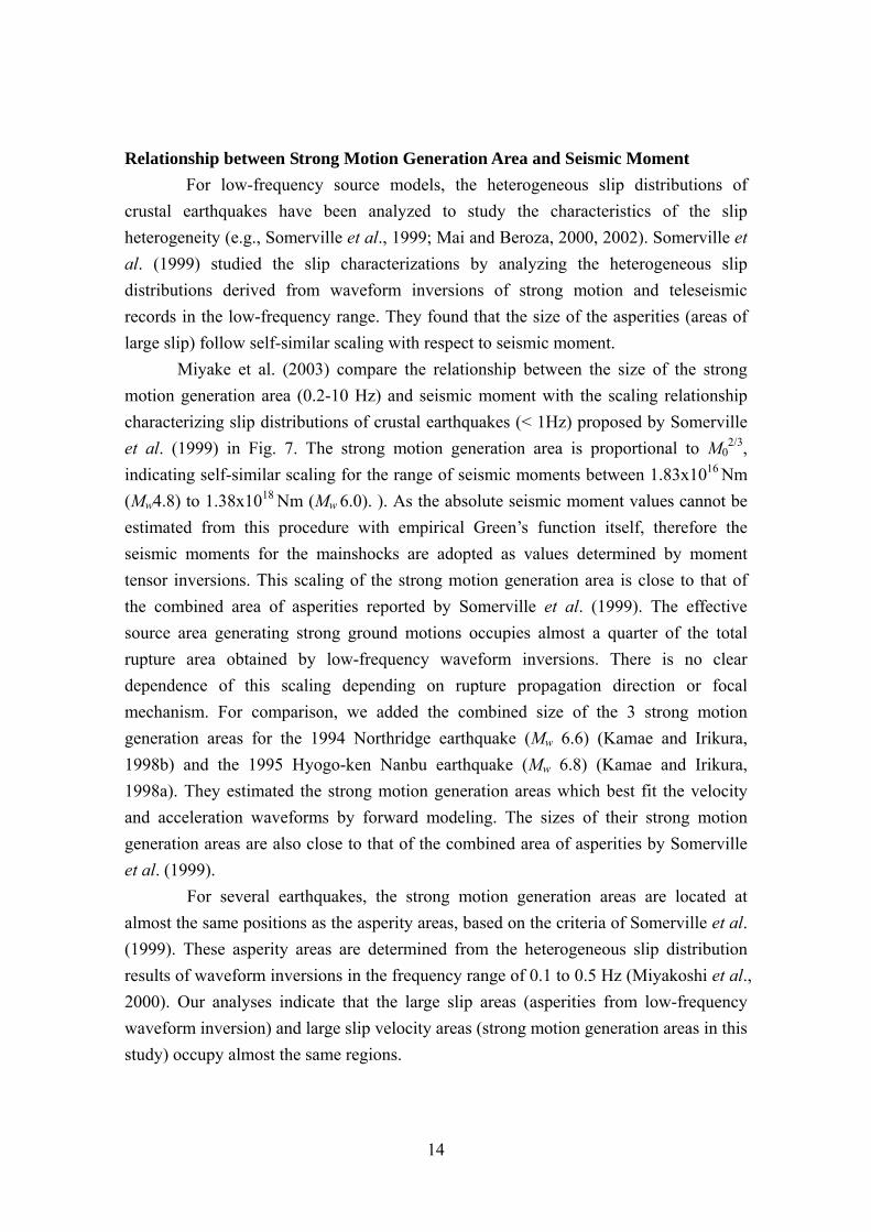
Relationship between Strong Motion Generation Area and Seismic Moment For low-frequency source models, the heterogeneous slip distributions of

crustal earthquakes have been analyzed to study the characteristics of the slip heterogeneity (e.g., Somerville et al., 1999; Mai and Beroza, 2000, 2002). Somerville et al. (1999) studied the slip characterizations by analyzing the heterogeneous slip distributions derived from waveform inversions of strong motion and teleseismic records in the low-frequency range. They found that the size of the asperities (areas of large slip) follow self-similar scaling with respect to seismic moment.

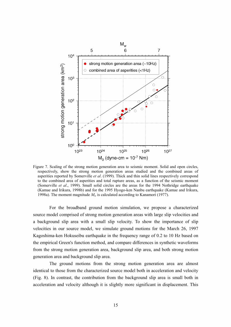
Miyake et al. (2003) compare the relationship between the size of the strong motion generation area (0.2-10 Hz) and seismic moment with the scaling relationship characterizing slip distributions of crustal earthquakes (< 1Hz) proposed by Somerville et al. (1999) in Fig. 7. The strong motion generation area is proportional to M0

2/3, indicating self-similar scaling for the range of seismic moments between 1.83x1016 Nm (Mw4.8) to 1.38x1018 Nm (Mw 6.0). ). As the absolute seismic moment values cannot be estimated from this procedure with empirical Green’s function itself, therefore the seismic moments for the mainshocks are adopted as values determined by moment tensor inversions. This scaling of the strong motion generation area is close to that of the combined area of asperities reported by Somerville et al. (1999). The effective source area generating strong ground motions occupies almost a quarter of the total rupture area obtained by low-frequency waveform inversions. There is no clear dependence of this scaling depending on rupture propagation direction or focal mechanism. For comparison, we added the combined size of the 3 strong motion generation areas for the 1994 Northridge earthquake (Mw 6.6) (Kamae and Irikura, 1998b) and the 1995 Hyogo-ken Nanbu earthquake (Mw 6.8) (Kamae and Irikura, 1998a). They estimated the strong motion generation areas which best fit the velocity and acceleration waveforms by forward modeling. The sizes of their strong motion generation areas are also close to that of the combined area of asperities by Somerville et al. (1999).

For several earthquakes, the strong motion generation areas are located at almost the same positions as the asperity areas, based on the criteria of Somerville et al. (1999). These asperity areas are determined from the heterogeneous slip distribution results of waveform inversions in the frequency range of 0.1 to 0.5 Hz (Miyakoshi et al., 2000). Our analyses indicate that the large slip areas (asperities from low-frequency waveform inversion) and large slip velocity areas (strong motion generation areas in this study) occupy almost the same regions.

15

Figure 7. Scaling of the strong motion generation area to seismic moment. Solid and open circles,

respectively, show the strong motion generation areas studied and the combined areas of asperities reported by Somerville et al. (1999). Thick and thin solid lines respectively correspond to the combined area of asperities and total rupture areas, as a function of the seismic moment (Somerville et al., 1999). Small solid circles are the areas for the 1994 Nothridge earthquake (Kamae and Irikura, 1998b) and for the 1995 Hyogo-ken Nanbu earthquake (Kamae and Irikura, 1998a). The moment magnitude Mw is calculated according to Kanamori (1977).

For the broadband ground motion simulation, we propose a characterized

source model comprised of strong motion generation areas with large slip velocities and a background slip area with a small slip velocity. To show the importance of slip velocities in our source model, we simulate ground motions for the March 26, 1997 Kagoshima-ken Hokuseibu earthquake in the frequency range of 0.2 to 10 Hz based on the empirical Green's function method, and compare differences in synthetic waveforms from the strong motion generation area, background slip area, and both strong motion generation area and background slip area.

The ground motions from the strong motion generation area are almost identical to those from the characterized source model both in acceleration and velocity (Fig. 8). In contrast, the contribution from the background slip area is small both in acceleration and velocity although it is slightly more significant in displacement. This

16

suggests that near-source strong ground motions are mainly controlled by the size of the strong motion generation area and its risetime.

Our characterized source model is constructed from the viewpoint of slip-velocity, and target frequency is 0.2-10 Hz. Miyakoshi et al. (2000) characterized the heterogeneous source model from the viewpoint of slip itself, and target frequency is 0.1-0.5 Hz. We showed that the characterized source model of slip in the low-frequency is equivalent to the characterized sourced model of slip-velocity in the broadband frequency.

Figure 8. Comparison of observed and synthetic waveforms (0.2-10 Hz) of the EW component at

station KGS002 for the 1997 Kagoshima-ken Hokuseibu earthquake, March. From top to bottom: Traces show observed waveforms, and synthetic waveforms from the strong motion generation area, both of strong motion generation area and background slip area in our characterized source model, and background slip area. From left to right: Acceleration, velocity, and displacement waveforms. Numbers above the waveforms are maximum amplitude values.

Conclusions

We estimated the strong motion generation area using the empirical Green’s function method, then confirmed that the strong motion generation areas coincide with the areas of the asperities of heterogeneous slip distributions derived from low-frequency (< 1 Hz) waveform inversions. The self-similar scalings for the size of the strong motion generation area and risetime, as a function of seismic moment are found for the range of earthquake less than Mw 6.0. These scalings are compatible with those for larger earthquakes obtained by Somerville et al. (1999).

Source characterization for simulating the broadband frequency ground motion requires strong motion generation areas which produce high-frequency motions with

17

large slip velocities as well as a background slip area which produces low-frequency motions with a small slip velocity. The near-source strong ground motions are controlled mainly by the size of the strong motion generation area and risetime there. The characterized source model looks different from the high-frequency source models from envelope inversions, however, we address that strong motion generation areas with 10 MPa stress drop can also reproduce a series of high-frequency waveforms.

Strong motion generation area contains both low- and high-frequency information which is scaled to the wave generations and rupture dynamics of small earthquake. We verified that quantified strong motion generation areas and the idea of the characterized source modeling have enough ability to perform the broadband ground motion simulation in acceleration, velocity, and displacement.

References Aki, K. (1967). Scaling law of seismic spectrum, J. Geophys. Res., 72, 1217-1231. Beroza, G. C. (1991). Near-source modeling of the Loma Prieta earthquake: evidence

for heterogeneous slip and implications for earthquake hazard, Bull. Seism. Soc. Am., 81, 1603-1621.

Bouchon, M., M. N. Toksöz, H. Karabulut, and M. -P. Bouin (2002). Space and time evolution of rupture and faulting during the 1999 İzmit (Turkey) earthquake, Bull. Seism. Soc. Am., 92, 256-266.

Boatwright, J. (1988). The seismic radiation from composite models of faulting, Bull. Seism. Soc. Am., 78, 489-508.

Brune, J. N. (1970). Tectonic stress and the spectra of seismic shear waves from earthquakes, J. Geophys. Res., 75, 4997-5009.

Brune, J. N. (1971). Correction, J. Geophys. Res., 76, 5002. Chi, W. C., D. Dreger, and A. Kaverina (2001). Finite-source modeling of the 1999

Taiwan (Chi-Chi) earthquake derived from a dense strong-motion network Bull. Seism. Soc. Am., 91, 1144-1157.

Cohee, B. P. and G. C. Beroza (1994). Slip distribution of the 1992 Landers earthquake and its implications for earthquake source mechanics, Bull. Seism. Soc. Am., 84, 692-172.

Cotton, F. and M. Campillo (1995). Frequency domain inversion of strong motions: Application to the 1992 Landers earthquake, J. Geophys. Res., 100, 3961-3975.

Das, S. and B. V. Kostrov (1986). Fracture of a single asperity on a finite fault: A model for weak earthquakes?, in Earthquake Source Mechanics (Geophysical Monograph Series Volume 37), S. Das, J. Boatwright, and C. H. Scholz (editors), American

18

Geophysical Union, Washington, D.C., 91-96. Delouis, B., D. Giardini, P. Lundgren, and J. Salichon et al. (2002). Joint inversion of

InSAR, GPS, teleseismic, and strong-motion data for the spatial and temporal distribution of earthquake slip: Application to the 1999 İzmit mainshock, Bull. Seism. Soc. Am., 92, 278-299.

Dziewonski, A. M., G. Ekstrom, and M. P. Salganik (1996). Centroid-moment tensor solutions for January-March 1995, Phys. Earth Planet. Interiors, 93, 147-157.

Dziewonski, A. M., G. Ekstrom, N. N. Maternovskaya, and M. P. Salganik (1997). Centroid-moment tensor solutions for July-September, 1996, Phys. Earth Planet. Interiors, 102, 133-143.

Faculty of Science, Kagoshima University (1997). The earthquakes with M6.3 (March 26, 1997) and with M6.2 (May 13, 1997) occurred in northwestern Kagoshima prefecture, Rep. Coord. Comm. Earthq. Pred., 58, 630-637 (in Japanese).

Faculty of Science, Kyushu University (1997). Seismic activity in Kyushu (November 1996-April 1997), Rep. Coord. Comm. Earthq. Pred, 58, 605-618 (in Japanese).

Fukuoka District Meteorological Observatory, JMA (1998). On an M6.3 earthquake in the northern Yamaguchi prefecture on June 25, 1997, Rep. Coord. Comm. Earthq. Pred, 59, 507-510 (in Japanese).

Fukuyama, E., M. Ishida, S. Horiuchi, H. Inoue, S. Hori, S. Sekiguchi, H. Kawai, H. Murakami, S. Yamamoto, K. Nonomura, and A. Goto (2000a). NIED seismic moment tensor catalogue January-December, 1999, Technical Note of the National Research Institute for Earth Science and Disaster Prevention, 199, 1-56.

Fukuyama, E., M. Ishida, S. Horiuchi, H. Inoue, S. Hori, S. Sekiguchi, A. Kubo, H. Kawai, H. Murakami, and K. Nonomura (2000b). NIED seismic moment tensor catalogue January-December, 1997, Technical Note of the National Research Institute for Earth Science and Disaster Prevention, 205, 1-35.

Fukuyama, E., M. Ishida, S. Horiuchi, H. Inoue, A. Kubo, H. Kawai, H. Murakami, and K. Nonomura (2001). NIED seismic moment tensor catalogue January-December, 1998 (revised), Technical Note of the National Research Institute for Earth Science and Disaster Prevention, 218, 1-51.

Graduate School of Science, Tohoku University (1999). On the seismic activity of the M6.1 earthquake of 3 September 1998 in Shizukuishi, Iwate prefecture, Rep. Coord. Comm. Earthq. Pred, 60, 49-53 (in Japanese).

Hartzell, S. H. (1978). Earthquake aftershocks as Green's functions, Geophys. Res. Lett., 5, 1- 4.

Harzell, S. H. and T. H. Heaton (1983). Inversion of strong ground motion and

19

teleseismic waveform data for the fault rupture history of the 1979 Imperial Valley, California, earthquake, Bull. Seism. Soc. Am., 73, 1553-1583.

Holland, J. H. (1975). Adaptation in natural and artificial systems, The University of Michigan Press, Ann Arbor.

Horikawa, H., K. Hirahara, Y. Umeda, M. Hashimoto, and F. Kusano (1996). Simultaneous inversion of geodetic and strong motion data for the source process of the Hyogo-ken Nanbu, Japan, earthquake, J. Phys. Earth, 44, 455-471.

Horikawa. H. (2001). Earthquake doublet in Kagoshima, Japan: Rupture of asperities in a stress shadow, Bull. Seism. Soc. Am., 91, 112-127.

Hurukawa, N. (1981). Normal faulting microearthquakes occurring near the moho discontinuity in the northeastern Kinki district, Japan, J. Phys. Earth, 29, 519-535.

Ide, S., M. Takeo, and Y. Yoshida (1996). Source process of the 1995 Kobe earthquake: determination of spatio-temporal slip distribution by Bayesian modeling, Bull. Seism. Soc. Am., 86, 547-566.

Ide, S. (1999). Source process of the 1997 Yamaguchi, Japan, earthquake analyzed in different frequency bands, Geophys. Res. Lett., 26, 1973-1976.

Irikura, K., Semi-empirical estimation of strong ground motions during large earthquakes, Bull. Disast. Prev. Res. Inst., Kyoto Univ., 33, 63-104, 1983.

Irikura, K. (1983). Semi-empirical estimation of strong ground motions during large earthquakes, Bull. Disast. Prev. Res. Inst., Kyoto Univ., 33, 63-104.

Irikura, K. (1986). Prediction of strong acceleration motions using empirical Green's function, Proc. 7th Japan Earthq. Eng. Symp., 151-156.

Irikura, K. and K. Kamae (1994). Estimation of strong ground motion in broad-frequency band based on a seismic source scaling model and an empirical Green's function technique, Annali di Geofisica, 37, 1721-1743.

Irikura, K., T. Kagawa, and H. Sekiguchi (1997). Revision of the empirical Green's function method by Irikura (1986), Programme and abstracts, Seism. Soc. Japan, 2, B25 (in Japanese).

Kakehi, Y. and K. Irikura (1996). Estimation of high-frequency wave radiation areas on the fault plane by the envelope inversion of acceleration seismograms, Geophys. J. Int., 125, 892-900.

Kakuta, T., H. Miyamachi, and A. Takagi (1991). Intermediate earthquakes in a northern part of the Kyushu-Ryukyu arc, Zisin, 44, 63-74 (in Japanese with English abstract).

Kamae, K. and K. Irikura (1998a). Source model of the 1995 Hyogo-ken Nanbu earthquake and simulation of near-source ground motion, Bull. Seism. Soc. Am., 88, 400-412.

20

Kamae, K. and K. Irikura (1998b). A source model of the 1994 Northridge earthquake (Mw=6.7), Proc. 10th Japan Earthq. Eng. Symp., 643-648 (in Japanese with English abstract).

Kanamori, H. (1977). The energy release in great earthquakes, J. Geophys. Res., 82, 2981-2987.

Kanamori, H. (1979). A semi-empirical approach to prediction of long-period ground motions from great earthquakes, Bull. Seism. Soc. Am., 69, 1645-1670.

Kanamori, H. and D. L. Anderson (1975). Theoretical basis of some empirical relations in seismology, Bull. Seism. Soc. Am., 65, 1073-1095.

Kawase, H. (1998). Metamorphosis of near-field strong motions by underground structures and their destructiveness to man-made structures – Learned from the damage belt formation during the Hyogo-ken Nanbu earthquake of 1995 –, Proc. 10th Japan Earthq. Eng. Symp., 29-34 (in Japanese with English abstract).

Kinoshita, S. (1998). Kyoshin Net (K-NET), Seism. Res. Lett., 69, 309-332. Kuge, K. (2003). Source modeling using strong-motion waveforms: Toward automated

determination of earthquake fault planes and moment-release distributions, Bull. Seism. Soc. Am., 93, 639-654.

Kuge, K., T. Iwata, and K. Irikura (1997). Automatic estimation of earthquake source parameters using waveform data from the K-NET, Programme and abstracts, Seism. Soc. Japan, 2, B16 (in Japanese).

Ma, K. F., J. Mori, S. J. Lee, and S. B. Yu (2001). Spatial and temporal distribution of slip for the 1999 Chi-Chi, Taiwan, earthquake, Bull. Seism. Soc. Am., 91, 1069-1087.

Madariaga, R., (1979). On the relation between seismic moment and stress drop in the presence of stress and strength heterogeneity, J. Geophys. Res., 84, 2243-2250.

Mai, P. M. and G. C. Beroza (2000). Source scaling properties from finite-fault rupture models, Bull. Seism. Soc. Am., 90, 604-615.

Mai, P. M. and G. C. Beroza (2002). A Spatial random-field model to characterize complexity in earthquake slip, J. Geophys. Res., 107, 10.1029/2001JB000588.

Miyake, H., T. Iwata, and K. Irikura (1999). Strong ground motion simulation and source modeling of the Kagoshima-ken Hokuseibu earthquakes of march 26 (MJMA6.5) and May 13 (MJMA6.3), 1997, using empirical Green's function method, Zisin, 51, 431-442 (in Japanese with English abstract).

Miyake, H., T. Iwata, and K. Irikura (2001). Estimation of rupture propagation direction and strong motion generation area from azimuth and distance dependence of source amplitude spectra, Geophys. Res. Lett., 28, 2727-2730.

Miyakoshi, K., T. Kagawa, H. Sekiguchi, T. Iwata, and K. Irikura (2000). Source

21

characterization of inland earthquakes in Japan using source inversion results, Proc. 12th World Conf. Earthq. Eng. (CD-ROM).

Miyamachi, H., K. Iwakiri, H. Yakiwara, K. Goto, and T. Kakuta (1999). Fine structure of aftershock distribution of the 1997 Northwestern Kagoshima earthquakes with a three-dimensional velocity model, Earth Planet Space, 51, 233-246.

Nakahara, H., T. Nishimura, H. Sato, and M. Ohtake (1998). Seismogram envelope inversion for the spatial distribution of high-frequency energy radiation from the earthquake fault: Application to the 1994 far east off Sanriku earthquake, Japan, J. Geophys. Res., 103, 855-867.

Nakahara, H., T. Nishimura, H. Sato, M. Ohtake, S. Kinoshita, and H. Hamaguchi (2002). Broad-band source process of the 1998 Iwate Prefecture, Japan, earthquake as revealed from inversion analyses of seismic waveforms and envelopes, Bull. Seism. Soc. Am., 92, 1708-1720.

Nakamura, H. and T. Miyatake (2000). An approximate expression of slip velocity time function for simulation of near-field strong ground motion, Zisin, 53, 1-9 (in Japanese with English abstract).

Ogue, Y., Y. Wada, A. Narita, and S. Kinoshita (1997). Deconvolution for the K-NET data from earthquake in southern Kyushu, Programme and abstracts, Seism. Soc. Japan, 2, B23 (in Japanese).

Okada, T., N. Umino, A. Hasegawa, and N. Nishide (1997). Source processes of the earthquakes in the border of Akita and Miyagi prefectures in August, 1996 (2), Programme and abstracts, Seism. Soc. Japan, 2, B69 (in Japanese).

Okada, T., N. Umino, Y. Ito, T. Matsuzawa, A. Hasegawa, and M. Kamiyama (2001). Source processes of 15 September 1998 M 5.0 Sendai, northeastern Japan, earthquake and its M 3.8 foreshock by waveform inversion, Bull. Seism. Soc. Am., 91, 1607-1618.

Satoh, T., H. Kawase, and S. Matsushima (1998). Source spectra, attenuation function, and site amplification factors estimated from the K-NET records for the earthquakes in the border of Akita and Miyagi prefectures in August, 1996, Zisin, 50, 415-429 (in Japanese with English abstract).

Sekiguchi, H., K. Irikura, T. Iwata, Y. Kakehi, and M. Hoshiba (1996). Minute locating of faulting beneath Kobe and the waveform inversion of the source process during the 1995 Hyogo-ken Nanbu, Japan, earthquake using strong ground motion records, J. Phys. Earth, 44, 473-487.

Sekiguchi, H., K. Irikura, and T. Iwata (2000). Fault geometry at the rupture termination of the 1995 Hyogo-ken Nanbu Earthquake, Bull. Seism. Soc. Am., 90, 117-133.

22

Sekiguchi, H. and T. Iwata (2002). Rupture process of the 1999 Kocaeli, Turkey, earthquake estimated from strong-motion waveforms, Bull. Seism. Soc. Am., 92, 300-311.

Somerville, P., K. Irikura, R. Graves, S. Sawada, D. Wald, N. Abrahamson, Y. Iwasaki, T. Kagawa, N. Smith, and A. Kowada (1999). Characterizing crustal earthquake slip models for the prediction of strong ground motion, Seism. Res. Lett., 70, 59-80.

Umino, N., T. Matsuzawa, S. Hori, A. Nakamura, A. Yamamoto, A. Hasegawa, and T. Yoshida (1998). 1996 Onikobe earthquakes and their relation to crustal structure, Zisin, 51, 253-264 (in Japanese with English abstract).

Wald, D. J., D. V. Helmberger, and T. H. Heaton (1991). Rupture model of the 1989 Loma Prieta earthquake from the inversion of strong motion and broadband teleseismic data, Bull. Seism. Soc. Am., 81, 1540-1572.

Wald, D. J. and T. H. Heaton (1994). Spatial and temporal distribution of slip of the 1992 Landers, California earthquake, Bull. Seism. Soc. Am., 84, 668-691.

Wald, D. J. (1996). Slip history of the 1995 Kobe, Japan, earthquake determined from strong motion, teleseismic, and geodetic data, J. Phys. Earth, 44, 489-503.

Wald, D. J., T. H. Heaton, and K. W. Hudnut (1996). The slip history of the 1994 Northridge, California, earthquake determined from strong-motion, teleseismic, GPS, and leveling data, Bull. Seism. Soc. Am., 86, S49-S70.

Wessel, P. and W. H. F. Smith (1995). New version of the Generic Mapping Tools released, EOS Trans. Am. Geophys. Union., 76, 329.

Wu. C., M. Takeo, and S. Ide (2001). Source process of the Chi-Chi earthquake: A joint inversion of strong motion data and global positioning system data with a multifault model, Bull. Seism. Soc. Am., 91, 1028-1043.

Yoshida, S., K. Koketsu, B. Shibazaki, T. Sagiya, T. Kato, and Y. Yoshida (1996). Joint inversion of near- and far-field waveforms and geodetic data for the rupture process of the 1995 Kobe earthquake, J. Phys. Earth, 44, 437-454.

Zeng, Y., K. Aki, and T. Teng (1993). Mapping of the high-frequency source radiation for the Loma Prieta earthquake, California, J. Geophys. Res., 98, 11981-11993.

Zeng, Y. and C. H. Chen (2001) Fault rupture process of the 20 September 1999 Chi-Chi, Taiwan, earthquake, Bull. Seism. Soc. Am., 91, 1088-1098.

23

Program of the empirical Green’s function method is available on the website below.

http://www.eri.u-tokyo.ac.jp/hiroe/EGF/

Kojiro Irikura E-mail: irikura@geor.or.jp Hiroe Miyake E-mail: hiroe@eri.u-tokyo.ac.jp

Hiroe Miyake and Kojiro Irikura

24

Chapter 3. Theoretical Simulation (3D FDM)

Summary

Long period ground motions are simulated using the fourth order finite difference method with a variable spacing staggered-grid by Pitarka (1999) and frequency-dependent attenuation factor (Graves, 1996). The calculations were performed in the frequency range of 0.05–0.4 Hz. Basin models in Osaka basin have been constructed by the geophysical and the geological data such as borehole, seismic reflection survey, microtremors and gravity anomaly data. Q value of sedimentary layers in Osaka Basin for long period ground motion are estimated by comparing synthetic motions including later phases with observed ones. The optimum Q value is given to be S-waves dependent as Q=f·Vs/2. Furthermore, we simulated long period ground motions in Osaka basin from great subduction-zone earthquakes occurring along the Nankai Trough.

Introduction

Osaka and Nagoya, representative mega cities of Japan, have repeatedly suffered from earthquake disasters caused by great subduction-zone earthquakes with magnitude more than 8 occurring along the Nankai Trough. The 30-year probability was estimated as 48 % and 61 % for the Nankai and Tonankai earthquakes, respectively, showing very high possibility of the earthquake occurrence. Osaka and Nagoya are located in basin with thick sediments (about 1 to 3 km), where long-period motions are strongly enhanced during those subduction-zone earthquakes.

There are lots of long period and low damping structures (such as tall buildings and oil tanks) inside the Osaka basin. It is very important for the earthquake disaster mitigation to predict the amplitude and duration of long period strong ground motions from the future Tonankai and Nankai earthquakes. To raise the precision of predicting long period ground motions, high accuracy three-dimensional (3D) velocity model and attenuation factor for sedimentary basin are required. The last few years, some 3D subsurface structure models of the Osaka sedimentary basin have been developed (Kagawa et al. (1993), Miyakoshi et al. (1999), Horikawa et al. (2003)). These models have been constructed by the geophysical and the geological data such as borehole, seismic reflection survey, microtremors and gravity anomaly data. However, these models can not accurately reproduce the seismic waveforms because of the lack of

25

sufficient investigation of the attenuation factor (Q value) and modeling using observed records. In this study, we focus on the Osaka basin, and try to optimize the Q value of sedimentary layers controlling mainly the amplitude of S-wave through the simulations of observed seismic waveforms. First of all, we construct the 3D velocity model of the Osaka basin referring to some data sets. Next, we search the optimum Q value of sedimentary layers from the fittings between the synthetic S-wave amplitudes and the observed ones of several actual earthquakes. Finally, we simulated long period ground motions in Osaka basin from great subduction zoon earthquake occurring along the Nankai Trough. Numerical Method

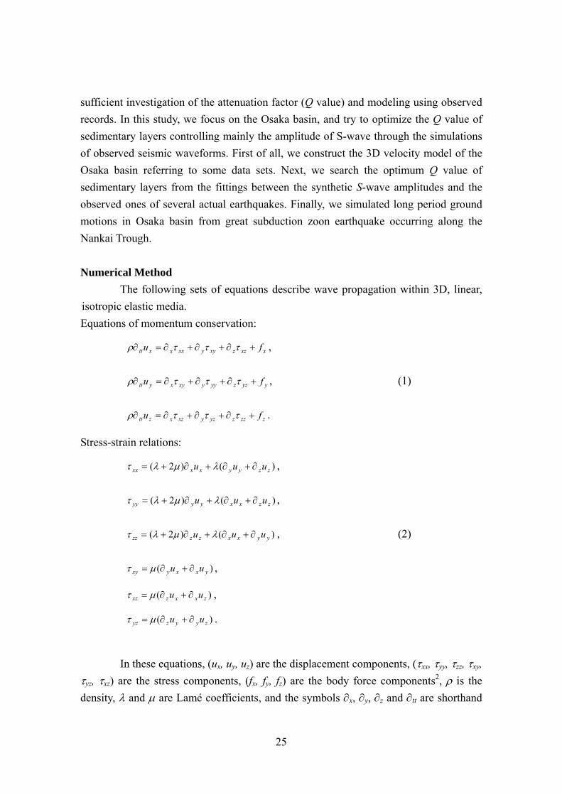
The following sets of equations describe wave propagation within 3D, linear, isotropic elastic media. Equations of momentum conservation:

xxzzxyyxxxxtt fu +∂+∂+∂=∂ τττρ ,

yyzzyyyxyxytt fu +∂+∂+∂=∂ τττρ , (1)

zzzzyzyxzxztt fu +∂+∂+∂=∂ τττρ .

Stress-strain relations:

)()2( zzyyxxxx uuu ∂+∂+∂+= λμλτ ,

)()2( zzxxyyyy uuu ∂+∂+∂+= λμλτ ,

)()2( yyxxzzzz uuu ∂+∂+∂+= λμλτ , (2)

)( yxxyxy uu ∂+∂= μτ ,

)( zxxzxz uu ∂+∂= μτ ,

)( zyyzyz uu ∂+∂= μτ .

In these equations, (ux, uy, uz) are the displacement components, (τxx, τyy, τzz, τxy,

τyz, τxz) are the stress components, (fx, fy, fz) are the body force components2, ρ is the density, λ and μ are Lamé coefficients, and the symbols ∂x, ∂y, ∂z and ∂tt are shorthand

26

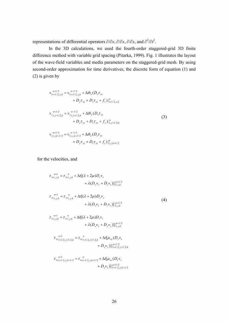
representations of differential operators ∂/∂x, ∂/∂x, ∂/∂x, and ∂2/∂t2. In the 3D calculations, we used the fourth-order staggered-grid 3D finite

difference method with variable grid spacing (Pitarka, 1999). Fig. 1 illustrates the layout of the wave-field variables and media parameters on the staggered-grid mesh. By using second-order approximation for time derivatives, the discrete form of equation (1) and (2) is given by

nkjixxzzxyy

xxxxn

kjixn

kjix

fDD

Dbtvv

,,2/1

2/1,,2/1

2/1,,2/1

|)

(

+

−+

++

+++

Δ+=

ττ

τ

nkjiyyzzyyy

xyxyn

kjiyn

kjiy

fDD

Dbtvv

,2/1,

2/1,2/1,

2/1,2/1,

|)

(

+

−

+

+

+

+++

Δ+=

ττ

τ (3)

nkjizzzzyzy

xzxzn

kjizn

kjiz

fDD

Dbtvv

2/1,,

2/12/1,,

2/12/1,,

|)

(

+

−+

++

+++

Δ+=

ττ

τ

for the velocities, and

2/1,,

,,1,,

|)](

)2[(+

+

++

+Δ+=n

kjizzyy

xxn

kjixxn

kjixx

vDvD

vDt

λ

μλττ

2/1,,

,,1,,

|)](

)2[(+

+

++

+Δ+=

nkjizzxx

yyn

kjiyyn

kjiyy

vDvD

vDt

λ

μλττ (4)

2/1,,

,,1,,

|)](

)2[(+

+

++

+Δ+=n

kjiyyxx

zzn

kjizzn

kjizz

vDvD

vDt

λ

μλττ

2/1,2/1,2/1

,2/1,2/11

,2/1,2/1

|)]

([+

++

++

+

++

+

Δ+=

nkjiyx

xyxyn

kjixyn

kjixy

vD

vDt μττ

2/12/1,,2/1

2/1,,2/11

2/1,,2/1

|)]

([+

++

+++

++

+

Δ+=n

kjizx

xzxzn

kjixzn

kjixz

vD

vDt μττ

27

2/12/1,2/1,

2/1,2/1,1

2/1,2/1,

|)]

([+

++

++

+

++

+

Δ+=

nkjizy

yzyzn

kjiyzn

kjiyz

vD

vDt μττ

for the stress. In these equations, the superscripts refer to the time index, and the subscripts refer to the spatial indices. Δt is the time step and Dx, Dy and Dz represent the central finite difference operators of the spatial derivatives ∂x, ∂y and ∂z, respectively.

The finite difference operators Dx, Dy, and Dz in computation are implemented on a mesh with nonuniform grid spacing developed by Pitarka (1999). We use effective parameters for the buoyancy b and the rigidity μ suggested by Graves (1996). This technique can significantly reduce computer memory and efficiently calculate ground motions at realistic 3-D structures at handling shorter wavelengths and larger areas than conventional ones as indicated by Pitarka (1999).

We set an absorbing region outside the finite computational region, and apply non-reflecting boundary condition of Cerjan et al. (1985) and the A1 absorbing boundary condition of Clayton and Engquist (1977) to the region. The implementation of the attenuation into the finite difference method is based on the Graves (1996) technique, which considers Q to be the same for both P and S waves, and frequency dependent, but the Q has the linear form

Q(f) = Q0 (f/f0), (5) where Q0 is the frequency-independent factor, f is the frequency, f0 is the reference frequency. In this study, the reference frequency was set at 1 Hz. Here, we assumed that the anelastic attenuation factor Q0 is proportional to the S-wave velocity, and given by

Q0 = α0 Vs, (6)

where α0 is the proportionality factor (s/m) and Vs is the S-wave velocity (m/s).

28

Figure 1. Grid layout for staggered-grid formulation. 3D Velocity Model and Verification

We try to produce a 3D velocity model of the Osaka Basin and estimate the optimum attenuation factors for long period ground motion simulation from the comparison between synthetic and observed waveforms. Our velocity model is constructed based on three data sets: (1) the background 3D crustal structure model, (2) the sedimentary-layer model of the Osaka basin by Miyakoshi et al. (1999) and Horikawa et al. (2003), and (3) the boundary between oceanic and land plates based on the Philippine See plate boundary model (hori et al., 2004). The area of our model, the epicenter of one of events (Table 1), and ground-motion-recording stations used in this study are shown in Fig. 2. The 3D bedrock topography in the corresponding area is shown in Fig. 3.

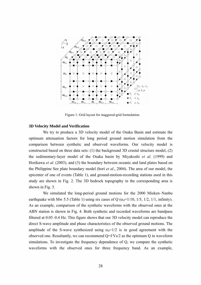
We simulated the long-period ground motions for the 2000 Mieken–Nanbu earthquake with Mw 5.5 (Table 1) using six cases of Q (α0=1/10, 1/5, 1/2, 1/1, infinity). As an example, comparison of the synthetic waveforms with the observed ones at the ABN station is shown in Fig. 4. Both synthetic and recorded waveforms are bandpass filtered at 0.05–0.4 Hz. This figure shows that our 3D velocity model can reproduce the direct S-wave amplitude and phase characteristics of the observed ground motions. The amplitude of the S-wave synthesized using α0=1/2 is in good agreement with the observed one. Resultantly, we can recommend Q=f·Vs/2 as the optimum Q in waveform simulations. To investigate the frequency dependence of Q, we compare the synthetic waveforms with the observed ones for three frequency band. As an example,

29

comparison of the synthetic waveforms using Q=f·Vs/2 with the observed ones at

Table 1. Source model of the Mieken–Nanbu earthquake

Origin Time Lon. Lat. Depth Strike Dip Rake Mo (JST) (°) (°) (km) (°) (°) (°) (Nm)

2000/10/31, 1:42 136.34 34.30 35.4 295.8 59.8 121.7 1.7×1017

Figure 2. A map showing the location of the epicenter shown in Table 1, observation stations, and the region of the sedimentary-layer model of the Osaka basin. The solid line indicates the location of the sedimentary layer model of the Osaka basin. the ABN station is shown in Fig. 5. The amplitudes and phases of the S-wave synthesized are in good agreement with the observed one for each frequency band. This result indicates that the Graves (1996) technique with Q=f·Vs/2 is available for actual frequency dependence of attenuation for the 0.05-0.4Hz frequency band.

Figure 3. 3D basement surface depth of the Osaka basin (Horikawa et al., 2003).

Epicenter

30

Figure 4. Comparison of the observed waveforms (blue line) with synthetic ones (pink line) of the Mieken-Nanbu earthquake for five cases of Q (Bandpass Filter: 0.05-0.4Hz)

Figure 5. Comparison of the observed waveforms (blue line) with synthetic ones (pink line) of the Mieken-Nanbu earthquake for three frequency band (Q=f·Vs/2)

31

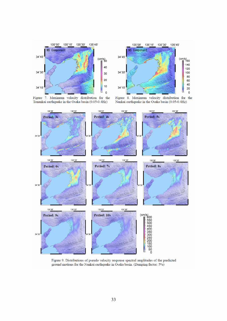
Prediction of Long Period Ground Motions Here, we tried to predict long-period ground motions for the future Tonankai

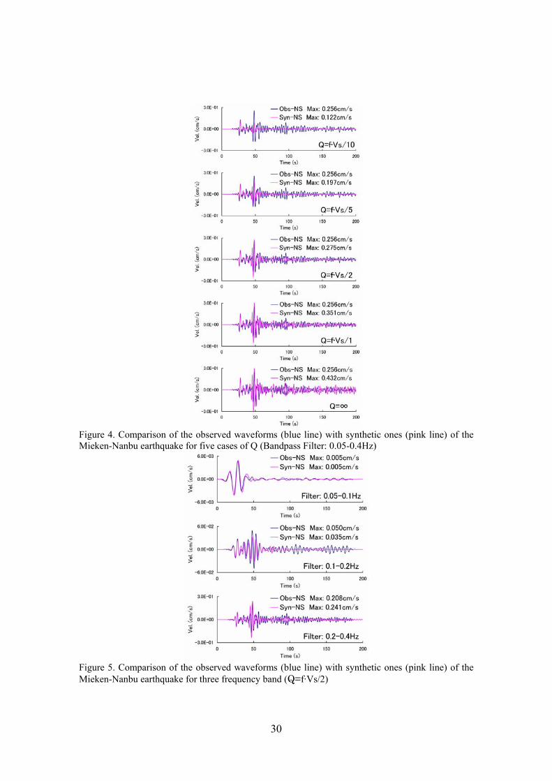
and Nankai earthquakes using the 3D finite difference method. We used a characterized source model proposed by Earthquake Research Committee (2005). The approach for the source characterization is based on the recipe for estimating strong ground motions from scenario earthquakes by Irikura et al. (2004). The location of the source region and the region for the 3D-FD simulation of the Tonankai and Nankai earthquakes are shown in Fig. 6.

Fig.7 and Fig.8 illustrate the maximum velocity distributions in the Osaka basin for the Tonankai and the Nankai earthquakes, respectively. The strong ground motion areas (red color area in Fig. 7) simulated for the Tonankai earthquake are different from those (Fig. 8) for the Nankai earthquake. The reason is that ground motion responses vary with incidental azimuth of seismic waves to the basins. Fig. 9 shows distributions of pseudo velocity response spectral amplitudes of the predicted ground motions for the Nankai earthquake in Osaka basin. Fig. 10 and Fig. 11 illustrate the velocity waveform and pseudo velocity response spectra at the FKS station shown in Fig. 3. Long period ground motions with periods of 4 to 6 second are mainly predominant in the Osaka basin. The characteristics of the long-period ground motions are related with the thicknesses of the sediments of the basins. The durations of long period ground motions inside the basin are more than 4 minutes. Acknowledgments

This work is supported by the Special Project for Earthquake Disaster Mitigation in Urban Areas from the Ministry of Education, Culture, Sports, Science and Technology of Japan. We used strong motion records observed by the Committee of Earthquake Observation and Research in Kansai Area (CEORKA), and F-net and KiK-net data of the National Institute for Earth Science and Disaster Research (NIED), Japan. The authors would like to thank these organizations.

32

(a) The region for the 3D-FD simulation of the Tonankai earthquake.

(b) The region for the 3D-FD simulation of the Nankai earthquake.

Figure 6. Maps showing the region of western Japan. The thick rectangular box depicts the region for the 3D-FD simulation of the Nankai and Tonankai earthquakes. The chain lines indicate the area of the velocity structure model of the Osaka basin and the Nobi basin. The contours show the isodepth lines of the Philippine Sea plate boundary.

33

34

Figure 10. Synthesized ground motion at FKS（Filter：0.05-0.4Hz）

Figure 11. Pseudo velocity response spectra with 5% damping at FKS

35

References Cerjan, C., D. Kosloff, R. Kosloff, and M. Reshef (1985). A nonreflecting boundary

condition for discrete acoustic and elastic wave equations, Geophysics, 50, 705-708. Clayton, R. and B. Engquist (1977). Absorbing boundary conditions for acoustic and

elastic wave equations, Bull. Seism. Soc. Am. 67, 1529-1540. Earthquake Research Committee (2005). 4. Seismic Hazard Maps for Specified Seismic

Faults, National Seismic Hazard Map for Japan (2005), http://www.jishin.go.jp/main/index-e.html, 59-61.

Graves, R. W. (1996). Simulating seismic wave propagation in 3D elastic media using staggered-grid finite differences, Bull. Seism. Soc. Am. 86, 1091–1106.

Hori, T., N. Kato, K. Hirahara, T. Baba, Y. Kaneda (2004). A numerical simulation of earthquake cycles along the Nankai Trough in southwest Japan: lateral variation in frictional property due to the slab geometry controls the nucleation position, Earth and Plan. Sci. Lett., 228, 215-226.

Horikawa, H., K. Mizuno, T. Ishiyama, K. Satake, H. Sekiguchi, Y. Kase, Y. Sugiyama, H. Yokota, M. Suehiro, T. Yokokura, Y. Iwabuchi, N. Kitada, A. Pitarka (2003). A three-dimensional model of the subsurface structure beneath the Osaka sedimentary basin, southwest Japan, with fault-related structural discontinuities. Annual Report on Active Fault and Paleoearthquake Researches, Geological Survey of Japan/AIST, 3, 225-259. (in Japanese with English abstract)

Irikura, K, H. Miyake, T. Iwata, K. Kamae, H. Kawabe, and L.A. Dalguer (2004). Recipe for predicting strong ground motions from future large earthquakes, 13th world conference of Earthquake Engineering, Vancouver, Canada, Paper No.1371.

Kagawa, T., S. Sawada, Y. Iwasaki, and A. Nanjo (1993). Modeling of deep sedimentary structure of the Osaka Basin, Proc. 22nd JSCE Eqrthq. Eng. Symp., 199-202 (in Japanese with English abstract).

Miyakoshi, K., T. Kagawa, B. Zhao, T. Tokubayashi and S. Sawada (1999). Modeling of deep sedimentary structure of the Osaka Basin (3), Proc. 25th JSCE Eqrthq. Eng. Symp., 185-188 (in Japanese with English abstract).

Pitarka, A. (1999). 3D elastic finite-difference modeling of seismic wave propagation using staggered grid with non-uniform spacing, Bull. Seism. Soc. Am. 89, 54–68.

Hidenori Kawabe, Katsuhiro Kamae, and Kojiro Irikura

36

Chapter 4.

Hybrid Method for Simulating Strong Ground Motion

Summary

Estimation of strong ground motions in the long-period range near a source area of a large earthquake have become possible as long as detailed slip distribution in its source fault and geological configurations from source to site are known. However, strong ground motions in the short-period range are difficult to calculate theoretically because of insufficient information about source and geological-structure. Then, hybrid methods for broad-band strong ground motions of engineering interest have been developed combining deterministic and stochastic approaches. Long-period motions from source faults of the large event are deterministically calculated using the 3-D finite-difference method. Short-period ground motions from small events occurring in the source area are stochastically simulated using Boore's method (1983). Short-period ground motions from the large event are estimated by following the empirical Green’s function method (Irikura, 1986). Finally, broad-band ground motions from the large event are synthesized summing the long-period and short-period motions after passing through a matched pair filter. Introduction

It is still difficult to compute numerically the Green’s functions at short-periods (< 1 sec.), i.e. at low frequencies (>1 Hz) of engineering interest. We need to know detailed geological configuration from source to site to compute such short-period motions. Even if it could be done, another problem is how to compute ground motions in such fine meshed 3-D structure. It is required to use so large memory and time-consumption in computing them.

If we have some records of small events occuring in the source areas of future large earthquakes, we can simulate strong ground motions in broad-band range from 0.1 to 10 sec. using the empirical Green’s function method (1986). However, in most of cases we do not have appropriate records from the small events enough to simulate them. Then, hybrid methods for broad-band strong ground motions of engineering interest have been developed combining deterministic and stochastic approaches. There are two kinds of methods to estimate strong ground motions from the large

37

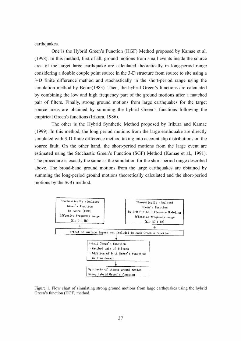
earthquakes. One is the Hybrid Green’s Function (HGF) Method proposed by Kamae et al.

(1998). In this method, first of all, ground motions from small events inside the source area of the target large earthquake are calculated theoretically in long-period range considering a double couple point source in the 3-D structure from source to site using a 3-D finite difference method and stochastically in the short-period range using the simulation method by Boore(1983). Then, the hybrid Green’s functions are calculated by combining the low and high frequency part of the ground motions after a matched pair of filters. Finally, strong ground motions from large earthquakes for the target source areas are obtained by summing the hybrid Green’s functions following the empirical Green's functions (Irikura, 1986).

The other is the Hybrid Synthetic Method proposed by Irikura and Kamae (1999). In this method, the long period motions from the large earthquake are directly simulated with 3-D finite difference method taking into account slip distributions on the source fault. On the other hand, the short-period motions from the large event are estimated using the Stochastic Green’s Function (SGF) Method (Kamae et al., 1991). The procedure is exactly the same as the simulation for the short-period range described above. The broad-band ground motions from the large earthquakes are obtained by summing the long-period ground motions theoretically calculated and the short-period motions by the SGG method.

Figure 1. Flow chart of simulating strong ground motions from large earthquakes using the hybrid Green’s function (HGF) method.

38

Method and Application Hybrid Green’s function method

The flow chart of the hybrid Green's function method (HGF method, hereafter) is presented in Figure 1. First, we simulate high frequency ground motion (f > 1 Hz) from a hypothetical small-event located in the fault plane of the target earthquake using the stochastic simulation technique of Boore (1983), assuming a point source. We introduce a frequency-dependent Q value to his specified acceleration spectrum. We can take into account additional factors such as the source mechanism (e.g. a double couple) and frequency-dependent radiation pattern (Pitarka et al., 2000). The Boore’s method is available only for simulating ground motions from the small-event but not for the large event because rupture propagation on the source fault is not taken into account. By using the Boore's method, the high frequency part of the simulated Green's function has an acceleration amplitude spectrum that follows the ω-2 model with the high-frequency cutoff (fmax=15 Hz). In the second step we calculate low frequency part of the Green's function (f < 1Hz) using the 3-D finite difference method, assuming a point source and adopting a 3-D velocity model of the heterogeneous structure. We apply a correction for the effect of the local surface layers not included in Boore's method as well as the 3-D calculation. After that, we calculate the hybrid Green's function by combining both the low and high frequency motions in time domain. A matched pair of filters is then used to remove the low (less than 1 Hz) and high frequency content (more than 1 Hz) from the stochastically simulated motion and the finite difference synthetic motion, respectively, and to follow the ω-2 spectral contents with respect to its source effect. Finally, strong ground motions from the large earthquake are simulated by the summation of the hybrid Green's functions following the EGF method by Irikura (1986).

We apply this method to simulating the ground motions from the 1995 Kobe Earthquake (Mw 6.9). The source model is assumed consisting of three asperities (No.1, 2, and 3) shown in Figure 2. The hybrid Green’s functions are calculated for three point sources located at the center of those three asperities assuming a magnitude 4.7 as almost coincided with the aftershock records used in the empirical Green’s function simulation (Kamae and Irikura, 1998).

For each point source, we assumed a pure right-lateral strike-slip mechanism with the strike and dip corresponding to each subfault. The map and station locations are shown in Figure 3. The basin velocity model used in the 3D finite-difference calculations includes a single sedimentary layer with the S wave velocity Vs=0.8 km/s, P wave velocity Vp=1.6 km/s, density ρ=2.1 g/cm3, constant attenuation factor Q=80,

39

and a background 1D velocity. The underground bedrock tomography is depicted in Figure 4.

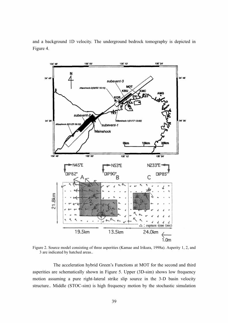
Figure 2. Source model consisting of three asperities (Kamae and Irikura, 1998a). Asperity 1, 2, and

3 are indicated by hatched areas.. The acceleration hybrid Green’s Functions at MOT for the second and third

asperities are schematically shown in Figure 5. Upper (3D-sim) shows low frequency motion assuming a pure right-lateral strike slip source in the 3-D basin velocity structure.. Middle (STOC-sim) is high frequency motion by the stochastic simulation

40

technique considering propagation-path effects due to a frequency-dependent Q factors (Qs= 33f) estimated from a linear inversion of ground motion spectra observed around the basin and local site effects from the 1-D structure modeling. Bottom (HYBRID) shows the hybrid Green’s function.

Figure 3. Map of the Kobe area and station locations. The locations of the heavily damaged zone are

shown by shadow. Solid triangles indicate the locations of mainshock observation stations (TKT, KOB, KBU, and MOT and aftershock observation stations (FKI and ASY). Solid lines show the surface intersections of the causative faults.

Figure 4. The bedrock topography in the Kobe area used in the 3-D finite-difference modeling (Pitarka et al., 1997b).

41

We show the comparison between the observed and synthesized seismograms (acceleration and velocity) at KBU, KOB, TKT, are MOT in Figure 6. The synthesized one at each station is selected among 20 simulations, that has the peak acceleration amplitude close to the simulated mean value. The standard deviation of the simulated peak amplitudes varies from 10 to 20 %. A comparison of the pseudo velocity response spectra are shown in Figure 7. Also shown in this figure is the variation (the mean value and the mean value plus/minus one standard deviation) of the response amplitude in short period range. The peak amplitudes of the simulated accelerations are close to those of the observed ones. The simulated velocity motions agree well with the observed ones.

Figure 5. An example of the entire procedure used for estimating the acceleration of hybrid Green’s

function. (a), (b), and (c) show the Green’s functions from, respectively, Number 1, 2, 3 hypothetical small events at MOT station. In each figure, “3D-sim” shows the corrected low frequency Green’s function, bandpass filtered between 0.2 and 1.0 Hz; “STOC-sim” shows the corrected high-frequency Green’s function, bandpass filtered between 1.0 and 10 Hz; and “HYBRID” shows the hybrid Green’s function obtained by seismograms.

42

Figure 6. Comparison between the synthetic acceleration and velocity seismograms (fault-normal

component) using hybrid Green’s functions and the observed ones from the mainshock. The seismograms are bandpass filtered between 0.2 and 10.0 Hz. The synthetic is the result of one of 20 simulations that has the peak acceleration amplitude close to the simulated mean value.

43

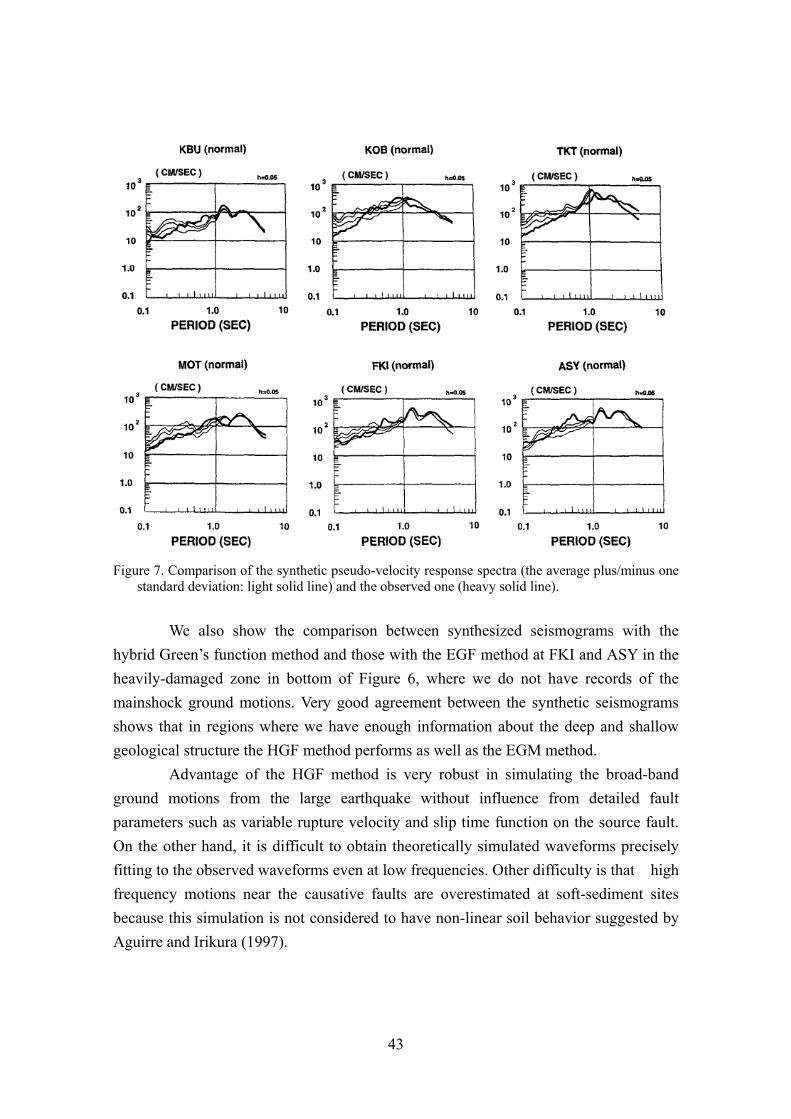
Figure 7. Comparison of the synthetic pseudo-velocity response spectra (the average plus/minus one

standard deviation: light solid line) and the observed one (heavy solid line).

We also show the comparison between synthesized seismograms with the hybrid Green’s function method and those with the EGF method at FKI and ASY in the heavily-damaged zone in bottom of Figure 6, where we do not have records of the mainshock ground motions. Very good agreement between the synthetic seismograms shows that in regions where we have enough information about the deep and shallow geological structure the HGF method performs as well as the EGM method.

Advantage of the HGF method is very robust in simulating the broad-band ground motions from the large earthquake without influence from detailed fault parameters such as variable rupture velocity and slip time function on the source fault. On the other hand, it is difficult to obtain theoretically simulated waveforms precisely fitting to the observed waveforms even at low frequencies. Other difficulty is that high frequency motions near the causative faults are overestimated at soft-sediment sites because this simulation is not considered to have non-linear soil behavior suggested by Aguirre and Irikura (1997).

44

The Hybrid Synthetic Method The flow chart of the hybrid synthetic method is shown in Figure 8. The

procedure for broad-band ground motion from the target large earthquake is slightly different from the HGF method. The low-frequency motions from the large earthquake are directly simulated with 3-D finite difference method taking into account slip distributions on the source fault and velocity structures extending from source to sites. On the other hand, the high-frequency ground motions from the large earthquake are estimated using the same technique as the empirical Green’s function method with stochastically simulated small-event motions instead of observed ones. After that, the low and high frequency ground motions simulated by those two methods are summed in time domain after passing through a pair of filters as shown in Figure 9.

Figure 8. Flow chart for simulating strong ground motions from large earthquakes using the hybrid

synthetic method. This method has been adopted in making “Seismic Hazard Maps for Specified

Seismic Source Faults, Japan (Earthquake Research Committee, 2005a). One of verifications of the method was done in simulating broad-band ground motions from the 2003 Tokachi-Oki earthquake with Mw 8.0, a great subduction-zone earthquake occurring off the Tokachi Region, Hokkaido, Japan (Earthquake Research Committee, 2005b; Morikawa et al., 2006). This earthquake provided a large amount of strong

45

motion records observed at more than 600 K-NET and Kik-NET stations. Those data are very helpful to verify the methodology of estimating strong ground motions by comparison of simulated results with observed results.

The map and observed stations are shown together with the source model in Figure 10. The rupture process of this earthquake are studied by many authors from waveform inversions using strong motion data (e.g. Honda et al.,2004) and teleseismic body-waves data (Yamanaka and Kikuchi, 2003), a joint inversion of strong motion and geodetic data (Koketsu et al., 2004), and so on. The location and geometry of the source fault is given from the aftershock distribution and the inversion results (e.g. Honda et al., 2004).

The outer fault parameters such as seismic moment and rupture area are estimated as follows. The seismic moment of 1.05x1021 Nm is estimated from the inversion results of the teleseismic data. The average stress drop is assumed to be 30 MPa (Kanamori and Anderson, 1975) and then the fault area is estimated to be 30x30 km2.

The inner fault parameters such as combined asperity areas and stress drop on asperities are estimated following the “Recipe” for subduction-zone earthquakes (e.g.Irikura, 2004). The number of the asperities and their locations are not given by the “Recipe”, but inferred by reference to the inversion results from the strong motion data (Honda et al., 2004) as shown in Figure 10.

The three-dimensional structure model is given based on the velocity profiles from the source area and the target area obtained reflection surveys. It is very important to accurate structure models with deep sediments for simulating strong ground motions. However, the information for modeling the 3-D structures is not enough to simulate ground motions higher than 0.2 Hz in this area. Therefore, the low frequency motions less than 0.2 Hz (longer than 5 seconds) here are theoretically simulated by the FDM, while the high frequency motions more than 0.2 Hz (shorter than 5 seconds) are simulated by the SGF method. The low and high frequency motions simulated above are first calculated on engineering bedrock (Vs = 400- 600 m/s). The ground motions on ground surface are calculated with a 1-D linear transfer functions due to soil-sediments between the engineering bedrock and surface.

We show an example of the comparison between the observed and simulated waveforms (velocity) at HKD129 in Figure 11. The uppermost two traces are the observed NS and EW components and the third one is the synthetic high frequency motions by the SGF method. The observed waveforms shown in the forth and fifth of Figure 11 ones are band-pass-filtered between 0.2 and 0.04 Hz (5 and 25 seconds) to

46

compare them with the low frequency motions theoretically simulated and the high frequency motions by the SGF method, both of which are band-pass-filtered in the same frequency range as the observed ones. A comparison of the pseudo velocity response spectra of the observed and simulated ones are shown in the bottom of Figure 11. We find that the theoretical waveforms and response-spectra agree well with the observed ones at periods between 5 and 25 seconds. The high frequency motions by the SGM method also coincide with the observed ones in spectral levels higher than 1 Hz, i.e. shorter than 1 second.

The totally synthesized motions are compared with the observed ones at three sites, TKCH11, HDKH05, and HKD093 very near the source fault in Fig. 12. We find that the synthesized motions at those sites agree well with the observe records. However, there are several stations where the theoretically simulated motions are not consistent with the observed ones in waveform and/or spectral level. One of the reasons is attributed to unreliability of the 3-D structure model. Another is that some fault parameters such as rupture velocity and slip time function are very sensitive to the ground motions in theoretical simulations. On the other hand high frequency motions by the SGF method are not sensitive to such fault parameters but strongly dependent on the inner fault parameters related to asperities such as location, size and stress drop.

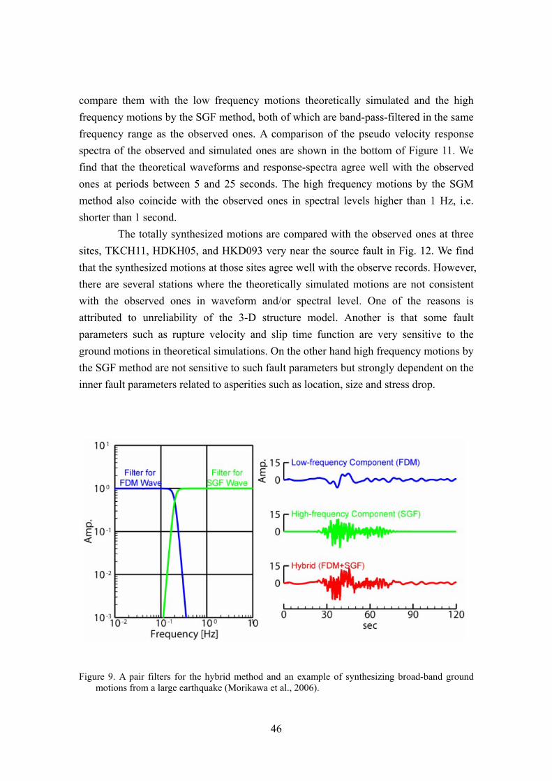
Figure 9. A pair filters for the hybrid method and an example of synthesizing broad-band ground

motions from a large earthquake (Morikawa et al., 2006).

47

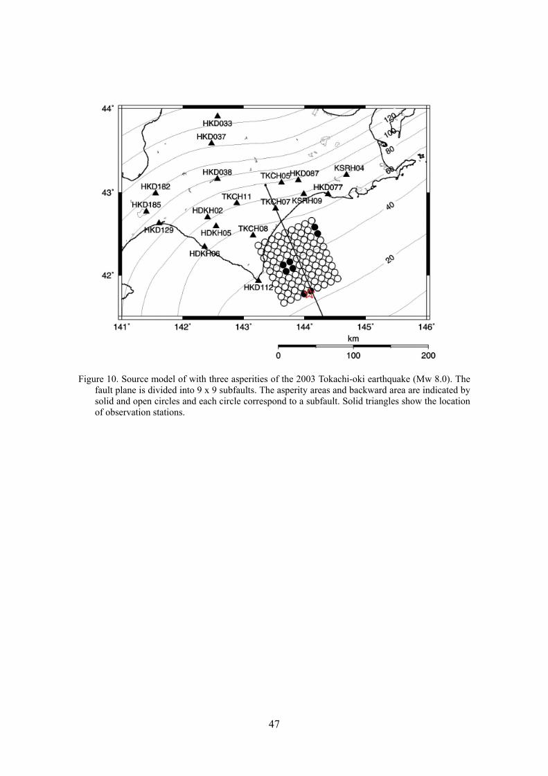
Figure 10. Source model of with three asperities of the 2003 Tokachi-oki earthquake (Mw 8.0). The

fault plane is divided into 9 x 9 subfaults. The asperity areas and backward area are indicated by solid and open circles and each circle correspond to a subfault. Solid triangles show the location of observation stations.

48

Figure 11. Comparison between observed motions (black) and simulated ones by theoretical method

(F.D.M.) (red) and by stochastic Green’s function method (green). Bottom two panels show the corresponding pseudo-velocity response spectra (5 % damping).

49

Fig. 12. Comparison of waveforms and pseudo-velocity-response spectra between observed and

synthesized. Conclusion

We introduce two methods for simulating broad band ground motions from large earthquakes, the hybrid Green’s function (HGF) method and the hybrid synthetic method.

In the HGF method, first the hybrid Green's function is estimated by combining low frequency motions by the finite-difference method and high frequency motions by stochastic method. After that, strong ground motions from the large earthquake are simulated by the summation of the hybrid Green's functions following the EGF method by Irikura (1986). This method was examined by comparing synthetic ground motions with observed records from 1995 Kobe earthquake (Mw=6.9). The comparison suggests that the HGF method is effective at simulating near-source ground motions in a broad-frequency range of engineering interest. Advantage of the HGF method is very robust in simulating the broad-band ground motions from the large earthquake without influence from detailed fault parameters such as variable rupture velocity and slip time function on the source fault. On the other hand, theoretically simulated waveforms are not precise enough to compare them with the observed waveforms even at low frequencies. One of other problems is that high frequency motions near the causative faults are overestimated at soft-sediment sites because this simulation is not considered to have non-linear soil behavior..

In the hybrid synthetic method, low frequency motions and high frequency

50

motions from the large earthquake are simulated separately, theoretically by the finite difference method and stochastically by the stochastic Green’s function method. After that, the low and high frequency ground motions simulated by those two methods are summed in time domain after passing through a pair of filters. This method was verified by comparing simulated broad-band ground motions with observed motions from the 2003 Tokachi-Oki earthquake with Mw 8.0. The totally synthesized motions agree well with the observe records at many stations near the source fault. However, there are some stations where the theoretically simulated motions are not consistent with the observed ones in waveform and/or spectral level. Reasons of discrepancy between the synthesized and observed motions are attributed to unreliability of the 3-D structure model as well as inaccuracy of rupture velocity and slip time function. On the other hand high frequency motions by the SGF method are not sensitive to such fault parameters but strongly dependent on the inner fault parameters related to asperities such as location, size and stress drop.

Acknowledgments

This study was done as a part of the governmental project of “National Seismic Hazard Map in Japan” sponsored by the Headquaters for Earthquake Research Promotion of Japan under the Ministry of Education, Culture, Sports, Science, and Technology. We express deep thanks for allowing me to refer the results and figures of the Seismic Hazard Map presented to the Earthquake Research Committee and to use the K-NET and Kik-NET data to the National Research Institute for Earth Science and Disaster Prevention (NIED), Japan. We would like to thank Katsuhiro Kamae to his contributions to this study. We also thank Nobuyuli Morikawa and NIED researchers for providing us their research results.

References Aguirre,J. and K. Irikura (1997). Nonlinearity, liquefaction, and velocity of soft soil

layers in Port Island, Kobe, during the Hyogo-ken Nanbu earthquake, Bull. Seism. Soc. Am., 87, 1244-1258.

Boore,D.M. (1983). Stochastic simulation of high-frequency ground motions based on seismological models of the radiated spectra, Bull. Seism. Soc. Am., 73, 1865-1894.

Graves,R. W. (1995). Preliminary analysis of long-period basin response in the Los Angeles region from the 1994 Northridge earthquake, Geophys. Res. Lett., 22, 101-104.

Earthquake Research Committee (2005a). National Seismic Hazard Map for Japan

51

(2005), Report published by the Headquarter of Earthquake Research Promotion under the Ministry of Education, Culture, Sports, Science, and Technology, 121p. (in Japanese).

Earthquake Research Committee (2005b). 4.3.13 Verification results using observed records of the 2003 Tokachi-Oki Earthquake, National Seismic Hazard Map for Japan (2005), http://www.jishin.go.jp/main/index-e.html

Hartzell, S.H. (1978). Earthquake aftershocks as Green's functions, Geophys. Res. Lett., 5, 1-4.

Hartzell, S., A. Leeds, A. Frankel, and J. Michael (1996). Site response for urban Los Angeles using aftershocks of the Northridge earthquake, Bull. Seism. Soc. Am., 86, S168-S192.

Heaton, T. H., J.F. Hall, D. J. Wald, and M. N. Halling (1995). Response of high-rise and base-isolated buildings to hypocetical Mw7.0 blind thrust earthquake, Science, 267, 206-211.

Honda, R., S. Aoi, N. Morikawa, H. Sekiguchi, K. Kunugi and H. Fujiwara (2004). Ground motion and rupture process of the 2003 Tokachi-oki earthquake obtained from strong motion data of the K-NET and KiK-net, Earth Planets and Space 56, 317-322.

Horikawa, H., K. Hirahara, Y. Umeda, M. Hashimoto, and F. Kusano (1996). Simultaneous inversion of geodetic and strong motion data for the source process of the Hyogo-ken Nanbu, Japan, earthquake, J. Physics Earth, 44, No.5, 455-472.

Ide, S. and M. Takeo (1996). Source process of the 1995 Kobe earthquake: Determination of spatio-temporal slip distribution by bayesian modeling, Bull. Seism. Soc. Am., 86, 547-566.

Irikura, K. (1986). Prediction of strong acceleration motion using empirical Green's function, Proc. 7th Japan Earthq. Symp.,151-156.

Iwata, T., K. Hatayama, H. Kawase, K. Irikura, and K. Matsushima (1995). Array observation of aftershocks of the 1995 Hyogoken-nanbu earthquake at Higashinada ward, Kobe city, J. Natural Disaster Science, 16, No.2, 41-48.

Iwata, T. ,K. Hatayama, H. Kawase, and K. Irikura (1996). Site amplification of ground motions during aftershocks of the 1995 Hyogo-ken Nanbu earthquake in severely damaged zone -Array observation of ground motions at Higashinada ward, Kobe city, Japan-, J. Physics Earth, 44, No.5, 553-562.

Kagawa,T., K. Irikura, and I. Yokoi (1996). Restoring clipped records of near-field strong ground motion during the 1995 Hyogo-ken Nanbu (Kobe), Japan earthquake, J. Natural Disast. Science, Vol.18, No.1, 43-57.

Kamae, K., P. Y. Bard, and K. Irikura (1998). Prediction of strong ground motion in a

52

EURO-SEISTEST using the empirical Green's function method, Journal of Seismology, 2, 193-207.

Kamae,K. and K. Irikura (1998). Source model of the 1995 Hyogo-ken Nanbu earthquake and simulation of near-source ground motion, Bull. Seism. Soc. Am., 88, 400-412.

Kawase,H. (1996). The cause of the damage belt in Kobe: "The basin edge effect", constructive interference of the direct S wave with the basin-induced diffracted/Rayleigh waves, Seis. Res. Lett., 67, No.5, 25-34.

Kinoshita, S. (1998). Kyoshin-net (K-NET), Seism. Res. Lett. 69, 309-332. Koketsu, K., K. Hikima, S. Miyazaki and S. Ide (2004). Joint inversion of strong motion

and geodetic data for the source rupture process of the 2003 Tokachi-oki, Hokkaido, earthquake, Earth Planets and Space 56, 329-334.

Morikawa, Aoi, Honda, Senna, Hayakawa, and Fujiwara (2006). Application of the ”recipe for strong ground motion evaluation” to the 2003 Tokachioki, Japan, earthquake, Third International Symposium on the Effects of Surface Geology on Seismic Motion, Paper Number 48.

Motosaka, M. and M. Nagano (1996). Analysis of ground motion amplification characteristics in Kobe city considering a deep irregular underground structue - Interpretation of Heavily damaged belt zone during the 1995 Hyogo-ken nanbu earthquake, J. Phys. Earth, 44, 577-590.

Nakamura, Y., F. Uehara, and H. Inoue (1996). Waveform and its analysis of the 1995 Hyogo-Ken-Nanbu earthquake (-6), JR Earthquake Information No,23d, Railway Technical Research Institute, March. (in Japanese)

Pitarka, A. and K. Irikura (1996). Basin structure effects on long period strong motions in the San Fernando valley and the Los Angeles Basin from the 1994 Northridge earthquake and an aftershock, Bull. Seism. Soc. Am., 86, S126-S137.

Pitarka, A., K. Irikura, T. Iwata, and T. Kagawa (1996). Basin structure effects in the Kobe area inferred from the modeling of ground motions from two aftershocks of the January 17, 1995 Hyogoken-nanbu eathquake, J. Physics Earth, 44, No.5, 563-576.

Pitarka, A., K. Irikura, and T. Iwata (1997a). Modeling of ground motion in Higashinada (Kobe) area for an aftershock of the January 17, 1995 Hyogo-ken Nanbu, Japan, earthquake, Geophys. J. Int. , 131, 231-239.

Pitarka, A., K. Irikura, T. Iwata, and H. Sekiguchi (1997b). Three-dimensional simulation of the near-fault ground motion for the 1995 Hyogo-ken Nanbu (Kobe), Japan earthquake, Bull. Seism. Soc. Am., 88, 428-440.

Pitarka, A., P. Somerville, Y. Fukushima, T. Uetake and K. Irikura (2000). Simulation of

53

Near-Fault Strong-Ground Motion Using Hybrid Green's Functions, Bull. Seism. Soc. Am., 90, 566-586.

Sekiguchi, H., K. Irikura, T. Iwata, Y. Kakehi, and M. Hoshiba (1996). Minute locating of faulting beneath Kobe and the waveform inversion of the source process during the 1995 Hyogo-ken Nanbu, Japan, earthquake using strong ground motion records, J. Physics Earth, 44, No.5, 473-488.

Wald, D. J. (1996). Slip history of the 1995 Kobe, Japan, earthquake determined from strong motion, teleseismic, and geodetic data, J. Physics Earth, 44, No.5, 489-504.

Yamanaka, Y. and M. Kikuchi (2003). Source process of the recurrent Tokachi-oki earthquake on September 26, 2003, inferred from teleseismic body waves, Earth Planets and Space 55, e21-e24.

Yoshida,S.,K. Koketsu, B. Shibazaki, T. Sagita, T.Kato, and Y. Yoshida (1996). Joint inversion of near- and far-field waveforms and geodetic data for the rupture process of the 1995 Kobe earthquake, J. Physics Earth, 44, No.5, 437-454.

Kojiri Irikura and Hiroe Miyake

54

Chapter 5. Recipe for Predicting Strong Ground Motion

Summary

A recipe for estimating strong ground motions from specific earthquakes is proposed based on source characteristics from the waveform inversion using strong motion data. Main features of the source model are characterized by three kinds of parameters, which we call: outer, inner, and extra fault parameters. The outer fault parameters are to outline the overall pictures of the target earthquakes such as entire source area and seismic moment. The inner fault parameters are parameters characterizing stress heterogeneity inside the fault area. The extra fault parameters are considered to complete the source model such as the starting point and propagation pattern of the rupture. The seismic hazard maps for future large earthquakes with high probability of occurrence potential are made following the idea of the recipe proposed here by two governmental organizations, the Head Quarter of Earthquake Research Center and Central Disaster Prevention Council in Japan. Introduction

From recent developments of the waveform inversion analyses for estimating rupture process using strong motion data during large earthquakes, we have understood that strong ground motion is relevant to slip heterogeneity inside the source rather than average slip in the entire rupture area. Asperities are characterized as regions that have large slip relative to the average slip on the rupture area, based on heterogeneous slip distributions estimated from the source inversion (Somerville et al., 1999). Then, they found that the asperity areas as well as entire rupture areas scale with total seismic moment. Another important study for strong motion prediction has been made that strong motion generation areas approximately coincide with the asperity areas where stresses are largely released (Miyake et al., 2001).

Based on the scaling relationships for the entire rupture area and asperity areas with respect to the total seismic moment, we found that the source model for the prediction of strong ground motions is characterized by three kinds of parameters, outer, inner, and extra fault parameters. The outer fault parameters are conventional parameters charactering earthquake sizes such as rupture area and seismic moment to outline the overall pictures of the source fault. So far, most of strong motion predictions in earthquake hazard analysis have been made using empirical attenuation-distance

55

curve for PGA (peak ground acceleration) and PGV (peak ground velocity) based on the outer fault parameters. However, from source inversion studies mentioned above we have realized that such parameters are not enough to estimate strong ground motions. The inner fault parameters are much more influential to strong ground motions, defining slip heterogeneity inside the source, that is, existence of asperities, area and stress drop of each asperity. The extra fault parameters are for characterizing rupture nucleation and termination such as the starting point and propagation pattern of the rupture.

We developed a “recipe” for predicting strong ground motions (Irikura and Miyake, 2001; Irikura et al., 2004), which is to characterize those three kinds of fault parameters for source modeling for the future large earthquakes. The idea of the “recipe” has been applied in the Seismic Hazard Map for Specified Seismic Source Faults by the Headquarters for Earthquake Research Promotion and the Central Disaster Prevention Council in Japan.

Strong Motion Prediction Program in Japan

The basic policy for defining the seismic hazard in Japan is based on the 1999 fundamental mission statement governing earthquake research over the next ten years as “The promotion of earthquake research – comprehensive basic policies for the promotion of seismic research through the observation, measurement, and survey of earthquakes –“, established by the Headquarters for Earthquake Research Promotion (Director: Ministry of Education,Culture, Sports, Science, and Technology). It initiated the creation of seismic hazard maps by promoting the survey of active faults, long-term evaluation of occurrence potentials and prediction of strong ground motion.

There were established two subcommittees under the Headquarter. One is for long term evaluation of earthquakes. The other is for strong motion evaluation that started in 1998 to make the seismic hazard maps from two different approaches, probabilistic and deterministic.

The probabilistic seismic hazard map is shown as the predicted likelihood of a ground motion level such as PGA, PGV, and seismic intensity occurring in a given area within a set period of time shown in Fig. 1. It provides important information for land planning, design standards of structures and people’s enlightening as to seismic risks.

The deterministic seismic hazard map is shown as the distribution of the ground motion level predicted for individual specific earthquakes assuming their fault models. The strong ground motions at specific sites near each source fault are estimated as time history, based on the recipe characterizing the source and numerical synthesis of waveforms with a hybrid scheme. Long-period motions are calculated with the finite

56

difference method considering the 3-D structures from the source to the target sites and short-period motions are simulated with the stochastic Green’s function method (e.g. Irikura and Kamae, 1999). Such time histories of the ground motions are useful for nonlinear dynamic analysis of structures, which is needed to design earthquake-resistant buildings and critical structures such as bridges, lifelines, electric power plants, and so on.

Fig. 1. Probability of suffering strong motion more than seismic intensity 6- within 30 years from

2005 AD (Earthquake Research Committee, 2005).

The Central Disaster Prevention Council belonging to the Cabinet Office also made seismic hazard maps for the Tokai, Tonankai and Nankai earthquakes shown as Fig. 2, which are feared likely to occur within the next half century. They made damage and causality estimates to determine disaster management plans for those earthquakes.

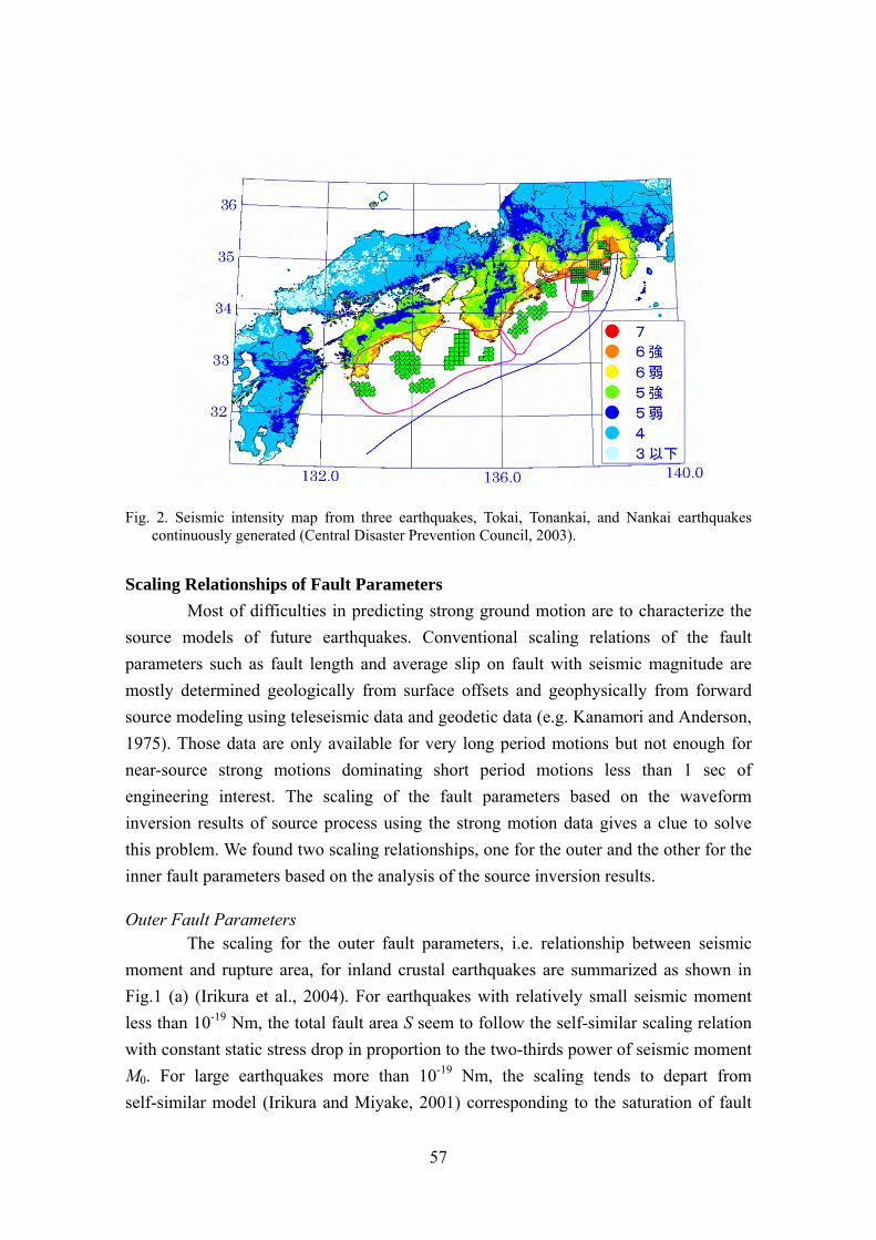
57

Fig. 2. Seismic intensity map from three earthquakes, Tokai, Tonankai, and Nankai earthquakes

continuously generated (Central Disaster Prevention Council, 2003). Scaling Relationships of Fault Parameters

Most of difficulties in predicting strong ground motion are to characterize the source models of future earthquakes. Conventional scaling relations of the fault parameters such as fault length and average slip on fault with seismic magnitude are mostly determined geologically from surface offsets and geophysically from forward source modeling using teleseismic data and geodetic data (e.g. Kanamori and Anderson, 1975). Those data are only available for very long period motions but not enough for near-source strong motions dominating short period motions less than 1 sec of engineering interest. The scaling of the fault parameters based on the waveform inversion results of source process using the strong motion data gives a clue to solve this problem. We found two scaling relationships, one for the outer and the other for the inner fault parameters based on the analysis of the source inversion results. Outer Fault Parameters

The scaling for the outer fault parameters, i.e. relationship between seismic moment and rupture area, for inland crustal earthquakes are summarized as shown in Fig.1 (a) (Irikura et al., 2004). For earthquakes with relatively small seismic moment less than 10-19 Nm, the total fault area S seem to follow the self-similar scaling relation with constant static stress drop in proportion to the two-thirds power of seismic moment M0. For large earthquakes more than 10-19 Nm, the scaling tends to depart from self-similar model (Irikura and Miyake, 2001) corresponding to the saturation of fault

58

width due to the seismogenic zone size. Such two-stage scaling relationship has been also found in Hanks and Bakun (2002). We add one more stage for extra large earthquakes more than 10-21 Nm from the idea of Scholtz (2002) as changing from L-model into W-model. The scaling relationships in this study as shown by broken lines in Fig.1 are drawn assuming the fault width saturates with 20 km long.

Fig. 3. Empirical relationships between seismic moment and rupture area for inland crustal

earthquakes (a) and subduction-zone earthquakes (b). Thick broken lines are 3-stage scaling

relationships proposed by our studies (e.g.，Irikura et al., 2004)

59

The three-stage scaling also seems to be applicable for subduction-zone earthquakes as shown in Fig. 1(b), although bending points are different. Saturation of the fault width for the subduction-zone earthquakes becomes longer.

Inner Fault Parameters Strong ground motions are influenced by inner fault parameters representing

slip heterogeneity more than outer fault parameters. The relationships between rupture area S as the outer fault parameter and combined area of asperities Sa as the inner fault parameter are shown in Fig.2 (Irikura et al., 2004). The ratio Sa / S seems to be constant regardless of the rupture area, about 0.22 for the inland earthquake and about 0.25 for the subduction earthquake. Then, stress drop on the asperities Δσa is derived as a multiple of the average stress drop over the fault cσΔ and the ratio of asperity area Sa to total rupture area S (e.g., Madariaga, 1979).

aca S

S⋅Δ=Δ σσ (1)

Another empirical-relationship between seismic moment Mo and acceleration source spectral level Ao related to the inner source parameters is shown in Fig. 3, originally found by Dan et al.(2001) and confirmed by other authors (Morikawa and Fujiwara, 2003; Satoh, 2004).

)(1046.2)( 3/10

170 cmdyneMcmdyneAa ⋅⋅⋅=⋅ (2)

The acceleration level Ao is theoretically related to the combined areas of asperities and the stress drop in the asperities for a circular asperity by Madariaga (1977).

aara SvA σβπ Δ= 40 (3)

By putting relationships 3/100 MA ∝ and 3/1

00 MA a ∝ obtained empirically (Irikura

and Miyake, 2001) together, the combined area of asperities are estimated as follows.

20

20

22

)()(

47

aRaAS

MvS

⋅⋅⎟

⎟⎠

⎞⎜⎜⎝

⎛= βπ

(4)

In this case the stress drop is also given by (1) .

60

Fig. 4. Empirical relationships between combined area of asperities and total rupture area (thick

broken line) for inland crustal earthquakes (left: after Irikura and Miyake, 2001) and subduction-zone earthquakes (right). Shadow ranges ± σ (standard deviation). Thin solid lines show a factor of 2 and 1/2 for the average. Database obtained by the waveform inversions for the inland crustal earthquakes is Somerville et al. (1999) and Miyakoshi (2002), for the subduction-zone earthquakes Somerville et al. (2002).

Fig. 5. Empirical relationship between seismic moment and acceleration source spectral level for

inland crustal earthquakes and for subduction-zone earthquakes.

61

Recipe for Source Modeling The procedure for characterizing the source model is outlined as a recipe for

estimating three kinds of source parameters, outer, inner, and extra fault parameters as follows: Outer Fault Parameters -Estimation of Seismic Moment for Possible Earthquake- Step 1: Total Rupture Area (S = LW)

Total fault length L of the possible earthquake is defined as sum of the lengths of the fault segments grouping simultaneously activated. Fault width W is related to the total fault length before reaching the thickness of the seismogenic zone Wmax and saturated at Wmax/sinθ, where θ is dip angle.

W (km) = L (km) for L < Wmax W (km) = Wmax/sin θ (km) for L >= Wmax (5)

Step 2: Total Seismic Moment (M0) The total seismic moment is estimated from the relationship between seismic moment and rupture area (Fig. 1(a) and (b)).

Step 3: Average Stress Drop ( cσΔ ) on the Fault Average static stress-drop for rupture area is estimated by a formula for circular

crack model by Eshelby (1957) in the first stage, then other formula considering tectonic loading stress (e.g., Fujii and Matsu’ura, 2000) at the second and third stages to naturally explain the 3-stage scaling relationships of seismic moment and rupture area.

Inner Fault Parameters - Slip Heterogeneity or Roughness of Faulting - Step 4. Combined Area of Asperities (Sa)

Two methods are used for combined areas of asperities. One is from the empirical relation of Sa-S (Somerville et al. 1999; Irikura and Miyake 2001), where the combined area of asperities is specified to be about 22%. The other is from equation (4) estimating the acceleration level from empirical relations or observed records.

Step 5. Stress Drop on Asperities ( aσΔ ) As shown in equation (1), aσΔ as the inner fault parameter is derived as a multiple of cσΔ as the outer fault parameter and Sa /S from Step 4.

Step 6. Number of Asperities (N) The asperities in the entire fault rupture are related to the segmentation of the active faults. Locations of the asperities are assumed from various kinds of

62

information such as surface offsets measured along fault, back-slip rate studied by GPS observation and weak reflection coefficients in fault plane.

Step 7: Average Slip on Asperities (Da) Based on Step 6 and empirical relationships from dynamic simulations of the slip distribution for the multiple-asperity source model (Dalguer et al, 2004). (Examples: Da /D = 2.3 for N = 1, Da /D = 2.0 for N = 2, Da /D = 1.8 for N =3 )

Step 8: Effective Stress on Asperity (σa) and Background Slip Areas (σb) Effective stress (σa) on asperity for strong motion generation is considered to be identical to stress drop on asperity ( aσΔ ). Effective stress on background slip area is constrained by the empirical relationship between seismic moment and acceleration source spectral level.

Step 9: Parameterization of Slip-Velocity Time Functions The Kostrov-like slip-velocity time functions are assumed as a function of peak slip-velocity and rise time based on the results of dynamic simulation by Day (1982). The peak slip-velocity is given as effective stress, rupture velocity and fmax.

Extra Fault Parameters - Propagation Pattern of Rupture -

The extra fault parameters are related to the fault geometry rupture starting point, characterizing rupture propagating pattern, and rupture velocity. For inland crustal earthquakes, rupture nucleation and termination are related to geomorphology of active faults (e.g., Nakata et al.,1998; Kame and Yamashita, 2003). For subduction-zone earthquakes, information from past earthquakes is applied as much as possible. Applicability and Validity of “Recipe”

The “recipe” proposed here has been applying to deterministic seismic-hazard maps for specified seismic source faults with high probability of occurrence potential in the National Seismic Hazard Maps for Japan (2005). The distribution of ground shaking levels such as PGV and seismic intensity has been evaluated for 10 inland crustal earthquakes and 2 subduction-zone earthquakes. The availability of the “recipe” has been tested in each application by the comparison between PGV’s of the synthesized motions and those derived from empirical attenuation relationship by Si and Midorikawa (1999).

More detailed examination has been attempted to show the validity and applicability of the “recipe” comparing simulated ground motions with observed ones for inland crustal earthquakes and subduction-zone earthquakes. We introduce two cases,

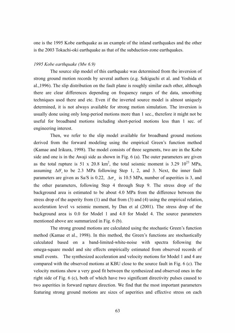
63

one is the 1995 Kobe earthquake as an example of the inland earthquakes and the other is the 2003 Tokachi-oki earthquake as that of the subduction-zone earthquakes. 1995 Kobe earthquake (Mw 6.9)

The source slip model of this earthquake was determined from the inversion of strong ground motion records by several authors (e.g. Sekiguchi et al. and Yoshida et al.,1996). The slip distribution on the fault plane is roughly similar each other, although there are clear differences depending on frequency ranges of the data, smoothing techniques used there and etc. Even if the inverted source model is almost uniquely determined, it is not always available for strong motion simulation. The inversion is usually done using only long-period motions more than 1 sec., therefore it might not be useful for broadband motions including short-period motions less than 1 sec. of engineering interest.

Then, we refer to the slip model available for broadband ground motions derived from the forward modeling using the empirical Green’s function method (Kamae and Irikura, 1998). The model consists of three segments, two are in the Kobe side and one is in the Awaji side as shown in Fig. 6 (a). The outer parameters are given as the total rupture is 51 x 20.8 km2, the total seismic moment is 3.29 1023 MPa, assuming cσΔ to be 2.3 MPa following Step 1, 2, and 3. Next, the inner fault parameters are given as Sa/S is 0.22, aσΔ is 10.5 MPa, number of asperities is 3, and the other parameters, following Step 4 through Step 9. The stress drop of the background area is estimated to be about 4.0 MPa from the difference between the stress drop of the asperity from (1) and that from (3) and (4) using the empirical relation, acceleration level vs seismic moment, by Dan et al (2001). The stress drop of the background area is 0.0 for Model 1 and 4.0 for Model 4. The source parameters mentioned above are summarized in Fig. 6 (b).

The strong ground motions are calculated using the stochastic Green’s function method (Kamae et al., 1998). In this method, the Green’s functions are stochastically calculated based on a band-limited-white-noise with spectra following the omega-square model and site effects empirically estimated from observed records of small events. The synthesized acceleration and velocity motions for Model 1 and 4 are compared with the observed motions at KBU close to the source fault in Fig. 6 (c). The velocity motions show a very good fit between the synthesized and observed ones in the right side of Fig. 6 (c), both of which have two significant directivity pulses caused to two asperities in forward rupture direction. We find that the most important parameters featuring strong ground motions are sizes of asperities and effective stress on each

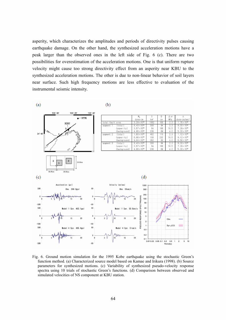
64

asperity, which characterizes the amplitudes and periods of directivity pulses causing earthquake damage. On the other hand, the synthesized acceleration motions have a peak larger than the observed ones in the left side of Fig. 6 (c). There are two possibilities for overestimation of the acceleration motions. One is that uniform rupture velocity might cause too strong directivity effect from an asperity near KBU to the synthesized acceleration motions. The other is due to non-linear behavior of soil layers near surface. Such high frequency motions are less effective to evaluation of the instrumental seismic intensity.

Fig. 6. Ground motion simulation for the 1995 Kobe earthquake using the stochastic Green’s

function method. (a) Characterized source model based on Kamae and Irikura (1998). (b) Source parameters for synthesized motions. (c) Variability of synthesized pseudo-velocity response spectra using 10 trials of stochastic Green’s functions. (d) Comparison between observed and simulated velocities of NS component at KBU station.

65

Variability of the synthesized pseudo-velocity response spectra calculated with 10 trials of the stochastic Greens functions is shown with the observed ones in Fig. 6 (d). The observed ones are ranged within one standard deviation at periods lower than 0.2 sec which are effective in measured seismic intensity. Large deviations of the synthesized motions at higher frequencies coincide with overestimation of the acceleration motions. We find that strong ground motions from the Kobe earthquake using the “recipe” are practically available to predict the distribution of seismic intensity. 2003 Tokachi-Oki Earthquake (Mw 8.0) So far, very few strong motion records from the seismic-zone earthquakes have been obtained over the world. Therefore, we have only less accurate inversion results of slip models of the subduction-zone earthquakes. The Tokachi-oki earthquake provided many strong ground motion records near the source area. Slip models for the earthquake have been proposed by several authors using strong motion records (e.g. Honda et al., 2004), teleseismic data (e. g. Yamanaka and Kikuchi, 2003), joint inversions of strong motion and teleseismic data (e.g. Yagi, 2004) and strong motion and geodetic data (Koketsu et al., 2004), and so on. Those results brought us a great opportunity to discuss the validity and applicability of the recipe to the subduction-zone earthquakes.

Verification of estimating strong ground motions for this earthquake based on “recipe” was shown in the National Seismic Hazard Map (2005) by Earthquake Research Committee (2005). We describe the outline of the verification mentioned above. The location and geometry of the seismic source fault is referred to Honda et al. (2004) as shown in the right bottom of Fig. 7. The rupture initiation point is taken at the epicenter determined by the Japan Meteorological Agency.

The order of setting the outer fault parameters is somewhat different from the inland earthquakes. The most stable and reliable parameter is seismic moment, which is adopted as 1.05 1021 N-m from the analysis of teleseismic data by Kikuchi and Yamanaka (2003). The rupture area is given to be 9000 km2, assuming cσΔ of 3.0 MPa (Kanamori and Anderson, 1975) in order of Step 2, Step 3 and Step 1 for the outer fault parameters.

The inner fault parameters are given as follows. First, the number of asperities is assumed to be three based on the source inversion results (Yamanaka and Kikuchi, 2003; Honda et al., 2004; Koketsu et al., 2004; Yagi, 2004). The locations of those three asperities are set as shown by solid circles inside the source fault in Fig. 7 referring the result from the forward modeling using the empirical Green’s function method by

66

Kamae and Kawabe (2004). The area of the large asperity is 361.2 km2 and that of the other two asperities is half of the large one. The stress drop of each asperity is estimated at 37.4 MPa from the empirical relation Mo vs acceleration level following Step 4 and 5. The rest of parameters are given with the “recipe”.

The synthesized motions are calculated using a hybrid method (Irikura and Kamae, 1999) with the crossover period of 5 sec, summing up longer period motions with a theoretical procedure and shorter period motions with the stochastic Green’s function method. Examples are shown in Fig. 7, in which waveforms and pseudo-velocity-response spectra are compared between the observed and synthesized motions at three sites, TKCH11, HDKH05, and HKD093 very near the source fault. We find that the synthesized motions agree well with the observe records.

The instrumental seismic intensity distributions estimated from the observed records and synthesized motions are shown in the left of Fig. 8. Comparison of the seismic intensity between the observed records and synthesized is shown in the right of Fig. 8. The seismic intensities from the synthesized motions are generally consistent with the observed ones. However, we can see overestimated synthesized motions in some regions where thick sedimentary layers are underlying. This might be due to the empirical formula of estimating instrumental seismic intensity from peak ground velocity. This formula tends to overestimate the instrumental seismic intensity with respect to ground motions having predominant longer than 2 sec.

There still remain many other problems to solve in applying the “recipe” to the subduction-zone earthquake. One of difficulties is to specify the number of asperities and places of them as long as no historical records exist. The other problems come from difficulties of lack of deep basin and off-shore structures from the source areas to objective regions, detailed geometries of plate boundaries, and so on.

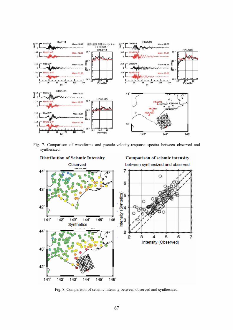
67

Fig. 7. Comparison of waveforms and pseudo-velocity-response spectra between observed and

synthesized.

Fig. 8. Comparison of seismic intensity between observed and synthesized.

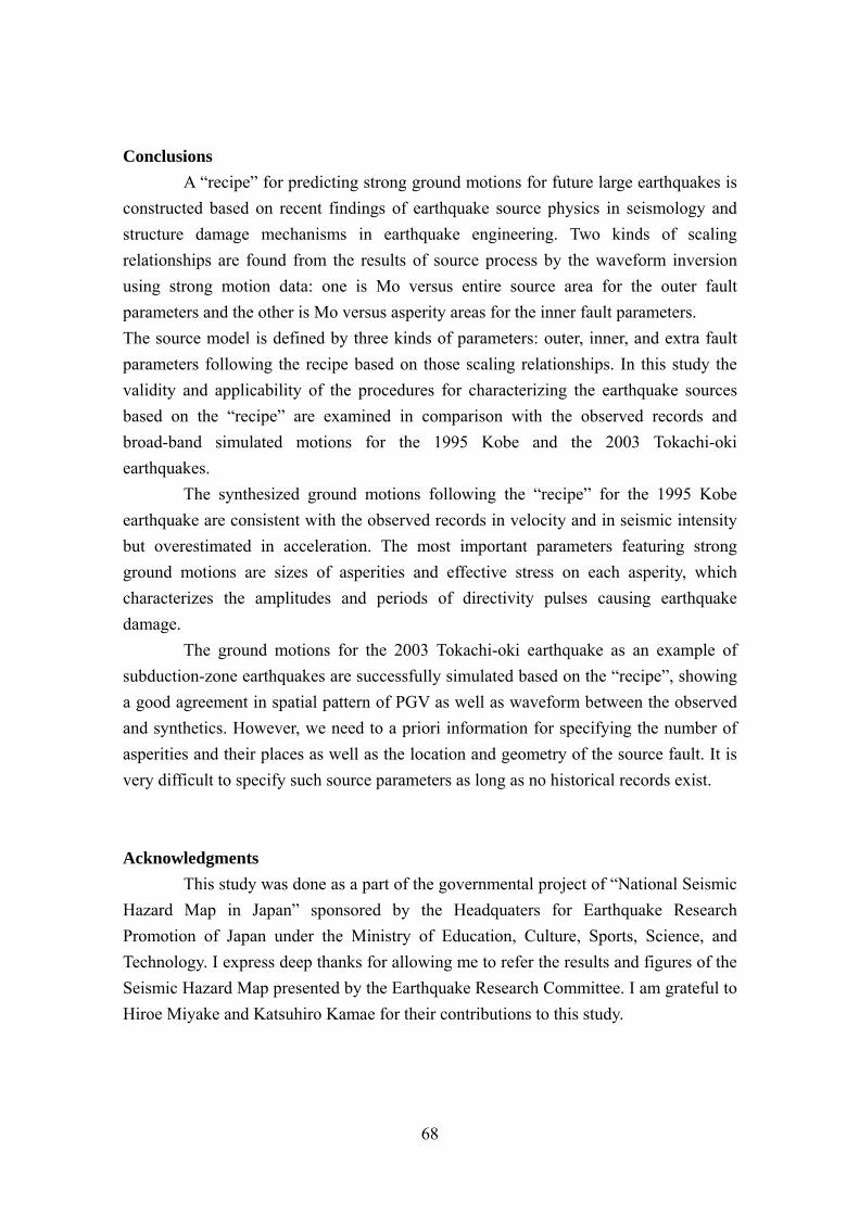
68

Conclusions A “recipe” for predicting strong ground motions for future large earthquakes is

constructed based on recent findings of earthquake source physics in seismology and structure damage mechanisms in earthquake engineering. Two kinds of scaling relationships are found from the results of source process by the waveform inversion using strong motion data: one is Mo versus entire source area for the outer fault parameters and the other is Mo versus asperity areas for the inner fault parameters. The source model is defined by three kinds of parameters: outer, inner, and extra fault parameters following the recipe based on those scaling relationships. In this study the validity and applicability of the procedures for characterizing the earthquake sources based on the “recipe” are examined in comparison with the observed records and broad-band simulated motions for the 1995 Kobe and the 2003 Tokachi-oki earthquakes.

The synthesized ground motions following the “recipe” for the 1995 Kobe earthquake are consistent with the observed records in velocity and in seismic intensity but overestimated in acceleration. The most important parameters featuring strong ground motions are sizes of asperities and effective stress on each asperity, which characterizes the amplitudes and periods of directivity pulses causing earthquake damage.

The ground motions for the 2003 Tokachi-oki earthquake as an example of subduction-zone earthquakes are successfully simulated based on the “recipe”, showing a good agreement in spatial pattern of PGV as well as waveform between the observed and synthetics. However, we need to a priori information for specifying the number of asperities and their places as well as the location and geometry of the source fault. It is very difficult to specify such source parameters as long as no historical records exist. Acknowledgments

This study was done as a part of the governmental project of “National Seismic Hazard Map in Japan” sponsored by the Headquaters for Earthquake Research Promotion of Japan under the Ministry of Education, Culture, Sports, Science, and Technology. I express deep thanks for allowing me to refer the results and figures of the Seismic Hazard Map presented by the Earthquake Research Committee. I am grateful to Hiroe Miyake and Katsuhiro Kamae for their contributions to this study.

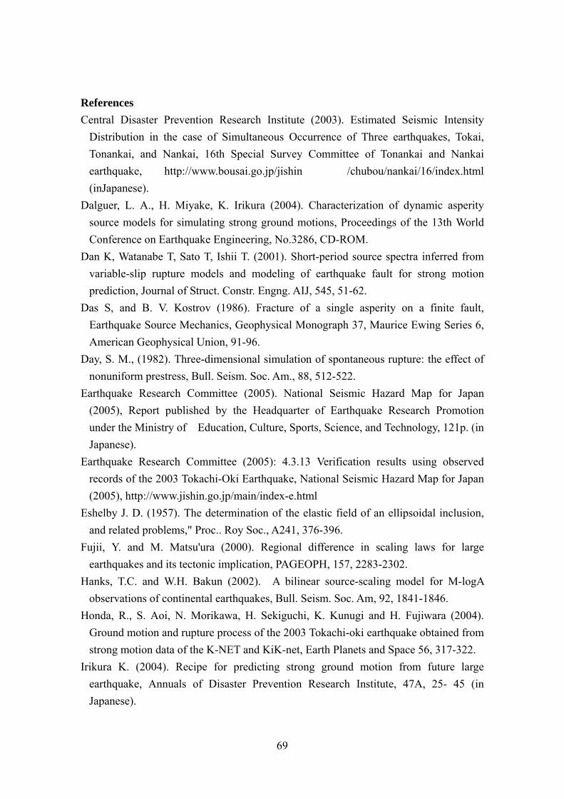
69

References Central Disaster Prevention Research Institute (2003). Estimated Seismic Intensity

Distribution in the case of Simultaneous Occurrence of Three earthquakes, Tokai, Tonankai, and Nankai, 16th Special Survey Committee of Tonankai and Nankai earthquake, http://www.bousai.go.jp/jishin /chubou/nankai/16/index.html (inJapanese).

Dalguer, L. A., H. Miyake, K. Irikura (2004). Characterization of dynamic asperity source models for simulating strong ground motions, Proceedings of the 13th World Conference on Earthquake Engineering, No.3286, CD-ROM.

Dan K, Watanabe T, Sato T, Ishii T. (2001). Short-period source spectra inferred from variable-slip rupture models and modeling of earthquake fault for strong motion prediction, Journal of Struct. Constr. Engng. AIJ, 545, 51-62.

Das S, and B. V. Kostrov (1986). Fracture of a single asperity on a finite fault, Earthquake Source Mechanics, Geophysical Monograph 37, Maurice Ewing Series 6, American Geophysical Union, 91-96.

Day, S. M., (1982). Three-dimensional simulation of spontaneous rupture: the effect of nonuniform prestress, Bull. Seism. Soc. Am., 88, 512-522.

Earthquake Research Committee (2005). National Seismic Hazard Map for Japan (2005), Report published by the Headquarter of Earthquake Research Promotion under the Ministry of Education, Culture, Sports, Science, and Technology, 121p. (in Japanese).

Earthquake Research Committee (2005): 4.3.13 Verification results using observed records of the 2003 Tokachi-Oki Earthquake, National Seismic Hazard Map for Japan (2005), http://www.jishin.go.jp/main/index-e.html

Eshelby J. D. (1957). The determination of the elastic field of an ellipsoidal inclusion, and related problems," Proc.. Roy Soc., A241, 376-396.

Fujii, Y. and M. Matsu'ura (2000). Regional difference in scaling laws for large earthquakes and its tectonic implication, PAGEOPH, 157, 2283-2302.

Hanks, T.C. and W.H. Bakun (2002). A bilinear source-scaling model for M-logA observations of continental earthquakes, Bull. Seism. Soc. Am, 92, 1841-1846.

Honda, R., S. Aoi, N. Morikawa, H. Sekiguchi, K. Kunugi and H. Fujiwara (2004). Ground motion and rupture process of the 2003 Tokachi-oki earthquake obtained from strong motion data of the K-NET and KiK-net, Earth Planets and Space 56, 317-322.

Irikura K. (2004). Recipe for predicting strong ground motion from future large earthquake, Annuals of Disaster Prevention Research Institute, 47A, 25- 45 (in Japanese).

70

Irikura K, and K. Kamae (1999). Strong ground motions during the 1948 Fukui earthquake, Zisin, 52, 129-150 (in Japanese).

Irikura K. and H. Miyake H. (2001). Prediction of strong ground motions for scenario earthquakes, Journal of Geography, 110, 849-875 (in Japanese with English abstract).

Kame N. and T. Yamashita T. (2003). Dynamic branching, arresting of rupture and the seismic wave radiation in self-chosen crack path modeling, Geophys. J. Int., 155, 1042-1050.

Kamae K. and K. Irikura (1998). Rupture process of the 1995 Hyogo-ken Nanbu earthquake and simulation of near-source ground motion, Bull. Seism. Soc. Am., 88, 400-412.

Kamae, K., K. Irikura, and A. Pitarka, 1998. A technique for simulating strong ground motion using hybrid Green's function, Bull. Seism. Soc. Am., 88, 357-367.

Kamae, K. and H. Kawabe (2004). Source model composed of asperities for the 2003 Tokachi-oki, Japan, earthquake (MJMA=8.0) estimated by the empirical Green's function method, Earth Planets and Space 56, 323-327.

Kanamori H. and D. L. Anderson (1975). Theoretical basis of some empirical relations in seismology, Bull. Seism. Soc. Am., 86, 1073-1095.

Kikuchi M. and Y. Yamanaka (2001). Rupture processes of past large earthquakes = Identification of asperities, Seismo, 5, 6-7.

Koketsu, K., K. Hikima, S. Miyazaki and S. Ide (2004). Joint inversion of strong motion and geodetic data for the source rupture process of the 2003 Tokachi-oki, Hokkaido, earthquake, Earth Planets and Space 56, 329-334.

Madariaga, R. (1977). High frequency radiation from crack (stress drop ) models of earthquake faulting, Geophys. J. R. Astron. Soc., 51, 625-651.

Madariaga, R., 1979. On the relation between seismic moment and stress drop in the presence of stress and strength heterogeneity, J. Geophys. Res., 84, 2243-2250.

Miyake, H., T. Iwata, and K. Irikura (2001). Estimation of rupture propagation direction and strong motion generation area from azimuth and distance dependence of source amplitude spectra, Geophys. Res. Lett., 28, 2727-2730.

Miyake H, T. Iwata, K. Irikura (2003). Source characterization for broadband ground motion simulation: Kinematic heterogeneous source model and strong motion generation area, Bull. Seism. Soc. Am., 93, 2531-2545.

Morikawa N. and H. Fujiwara (2003). Source and path characteristics for off Tokachi-Nemuro earthquakes, Programme and Abstracts for the Seismological Society of Japan, 2003 Fall Meeting, 104 (in Japanese).

Nakata T, Shimazaki K, Suzuki Y, Tsukuda E. (1998). Fault branching and directivity of

71

rupture propagation, Journal of Geography, 107, 512-528 (in Japanese). Satoh T. (2004). Short-period spectral level of intraplate and interplate earthquakes

occurring off Miyagi prefecture, Journal of JAEE’2004, 4, 1-4 (in Japanese with English abstract).

Scholz C. H. (2002). The mechanics of earthquakes and faulting, Cambridge University Press.

Sekiguchi, H., Irikura, K., and Iwata, T. (2000): Fault geometry at the rupture termination of the 1995 Hyogo-ken Nanbu earthquake, Bull. Seism. Soc. Am., 90, 974-1002.

Si, H. and S. Midorikawa (1999). New attenuation relationships for peak ground acceleration and velocity considering effects of fault type and site condition, J. Struct. Constr. Eng., AIJ, 523, 63-70 (in Japanese with English abstract).

Somerville P, K. Irikura, R. Graves, S. Sawada, D. Wald, N. Abrahamson, Y. Iwasaki, T. Kagawa, N. Smith, A. Kowada (1999). Characterizing earthquake slip models for the prediction of strong ground motion, Seism. Res. Lett., 70, 59-80.

Yagi, Y. (2004). Source rupture process of the 2003 Tokachi-oki earthquake determined by joint inversion of teleseismic body wave and strong ground motion data, Earth Planets and Space 56, 311-316.

Yamanaka Y, M. Kikuchi M (2003). Source process of the recurrent Tokachi-oki earthquake on September 26, 2003,inferred from teleseismic body waves, Earth Planets Space, 55,e21–e24.

Yoshida, S., K. Koketsu, B. Shibazaki, T. Sagiya, T. Katoand Y. Yoshida (1996). Joint inversion of the near- and far-field waveforms and geodetic data for the rupture process of the 1995Kobe earthquake, J. Phys. Earth, 44, 437--454, 1996.

Kojiri Irikura and Hiroe Miyake