Stripe Parameterization of Tubular Surfaces

Felix Kalberer, Matthias Nieser, and Konrad Polthier

Freie Universitat Berlin

Abstract. We present a novel algorithm for automatic parameteriza-tion of tube-like surfaces of arbitrary genus such as the surfaces of knots,trees, blood vessels, neurons, or any tubular graph with a globally con-sistent stripe texture. Mathematically these surfaces can be described asthickened graphs, and the calculated parameterization stripe will followeither around the tube, along the underlying graph, a spiraling combi-nation of both, or obey an arbitrary texture map whose charts have a180 degree symmetry.We use the principal curvature frame field of the underlying tube-likesurface to guide the creation of a global, topologically consistent stripeparameterization of the surface. Our algorithm extends the QuadCoveralgorithm and is based, first, on the use of so-called projective vectorfields instead of frame fields, and second, on different types of branchpoints. That does not only simplify the mathematical theory, but alsoreduces computation time by the decomposition of the underlying stiff-ness matrices.

1 Introduction

Tubular surfaces appear in many application areas such as networks of bloodvessels and neurons in medicine, or tube and hose systems in industrial environ-ments. Often a tubular structure must be recovered and segmented from noisyscan data. Our stripe parameterizer is an efficient and automatic method for theparameterization and remeshing of free-form tubular surfaces given as trianglemeshes. Our special focus lies on free-form surfaces which are not made out ofregular, cylindrical tube pieces - those can be handled better by other algorithmsfrom CAD. An additional benefit of the stripe parameterization is the enhancedvisualization of the underlying geometric structure.

1.1 Previous work

Surface parameterization is an active research area. We will not attempt a com-plete review of the literature but instead refer the reader to the surveys byFloater and Hormann [1] and [2].

A very early surface parameterization method is the Tutte’s [3] barycentricgraph embedding. Tutte embeddings are of combinatorial structure and do notcapture the geometry of the surface. Early global parameterization methods wereintroduced by Haker, Gu and Yau [4–6] who studied conformal parameteriza-tions. Conformal maps are angle preserving at the cost of possibly large lengthdistortions, as angles and lengths can not be preserved at the same time.

To reduce length distortion, Kharevych et al. [7] used cone singularities forconformal parameterization, which relax the constraint of a flat parameter do-main at few isolated points. Such singularities have proven to be essential forhigh quality parameterizations and have been used in other parameterizationschemes as well.

Tong et al. [8] use singularities at the vertices of a hand-picked quadrilateralmeta layout on the surface. The patches the meta layout are then parameterizedby solving for a global harmonic one form. Dong et al. [9] use a similar idea forparmeterization but create the quadrilateral meta layout automatically from theMorse-Smale complex of eigenfunctions of the mesh Laplacian.

Ray et al. [10] parameterize surfaces of arbitrary genus with periodic po-tential functions guided by two orthogonal input vector fields. This leads to acontinuous parameterization except in the vicinity of singular points on the sur-face. These singular regions are detected and reparameterized afterwards. Withthe QuadCover algorithm [11] we built upon their idea to use an input field asguiding directions for parameter lines. Input fields can be principal curvaturedirections, for example, or user-designed fields using one of the recent tools forthe design of rotational symmetry fields like [12], [13], [14], or [15]. The ideaof QuadCover is to find a parameterization whose gradient matches the inputdirections as well as possible.

The literature on parameterization of tubular objects is by far not as exten-sive as for general surfaces. Huysmans et al. [16] construct a progressive meshwhich they map to an open cylinder. A subsequent iterative scheme optimizesthe vertex positions in the cylindrical domain. Unfortunately, that method cannot handle bifurcations. Antiga and Steinman [17] handle blood vessels with bi-furcations by splitting the vessel tubes at their branches, and parameterize eachsegment separately which leaves visible artifacts at the joints of the segments.Zhu et al. [18] use conformal parameterizations on tubular objects. Since con-formal maps do not allow precise control over the direction of parameter lines,they cannot be aligned with the tube axis.

1.2 Contributions

We introduce the stripe parameterizer, an algorithm for the generation of glob-ally consistent stripe parameterizations, see Fig. 1 and 9. Each parameterizationis a collection of texture maps which may also be used to remesh and segmenta surface. The stripe parameterizer is a generalization of QuadCover, whichparameterizes general surface meshes. The stripe parameterizer allows to mapstripe patterns onto a surface, i. e., texture maps whose individual charts aresymmetric with respect to rotations of 180 degrees. In contrast to QuadCoverwhere all texture image charts have to be symmetric with respect to 90 degreerotations, the stripe parameterizer allows a more general set of texture imageswith only 180 degree symmetry.

We develop the mathematical theory for stripe parameterizations and discussthe differences to grid parameterization techniques including those in Quad-Cover. Stripe parameterizations allows only a subset of the branch point types

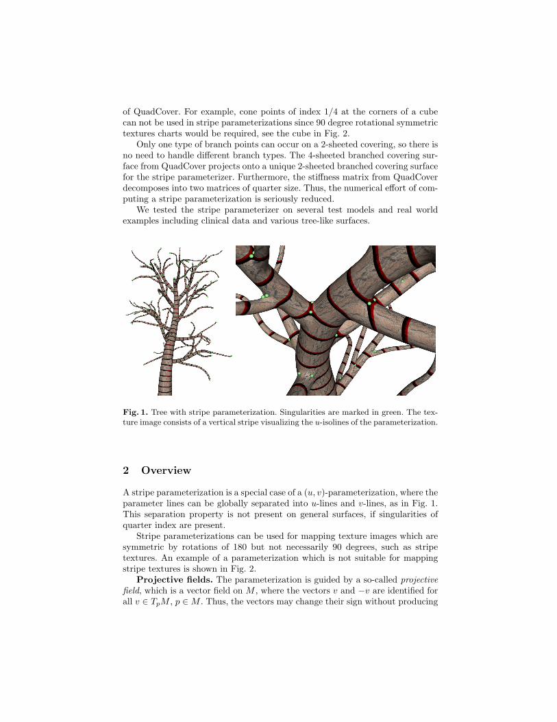
of QuadCover. For example, cone points of index 1/4 at the corners of a cubecan not be used in stripe parameterizations since 90 degree rotational symmetrictextures charts would be required, see the cube in Fig. 2.

Only one type of branch points can occur on a 2-sheeted covering, so there isno need to handle different branch types. The 4-sheeted branched covering sur-face from QuadCover projects onto a unique 2-sheeted branched covering surfacefor the stripe parameterizer. Furthermore, the stiffness matrix from QuadCoverdecomposes into two matrices of quarter size. Thus, the numerical effort of com-puting a stripe parameterization is seriously reduced.

We tested the stripe parameterizer on several test models and real worldexamples including clinical data and various tree-like surfaces.

Fig. 1. Tree with stripe parameterization. Singularities are marked in green. The tex-ture image consists of a vertical stripe visualizing the u-isolines of the parameterization.

2 Overview

A stripe parameterization is a special case of a (u, v)-parameterization, where theparameter lines can be globally separated into u-lines and v-lines, as in Fig. 1.This separation property is not present on general surfaces, if singularities ofquarter index are present.

Stripe parameterizations can be used for mapping texture images which aresymmetric by rotations of 180 but not necessarily 90 degrees, such as stripetextures. An example of a parameterization which is not suitable for mappingstripe textures is shown in Fig. 2.

Projective fields. The parameterization is guided by a so-called projectivefield, which is a vector field on M , where the vectors v and −v are identified forall v ∈ TpM , p ∈M . Thus, the vectors may change their sign without producing

Fig. 2. QuadCover parameterization with quad texture and stripe texture. Stripe tex-tures can not simply be used in parameterizations from QuadCover.

a discontinuous projective field. Note, that projective fields are a special case ofN -RoSy fields for N = 2 as introduced by Palacios and Zhang [13].

The algorithm takes two projective fields as input and generates two scalarfunctions (u and v), whose gradients match up with the input fields as well aspossible. The coordinates u and v can be used as texture coordinates in orderto map a pattern onto the surface. If you are only interested in a stripe pattern,you could use only one input field and skip the computation of v.

Construct an input field. It is up to the user to construct an input field.A canonical choice is the field of minimum curvature: In each point, the corre-sponding vector points in direction of the (absolute) smaller principle curvatureand has unit length. Using this field (together with the 90 degrees rotated field)as the input fields yields nearly curvature line parameterizations.

The algorithm. Starting from a given projective field, the algorithm firstconstructs a locally integrable field. Second, the surface is cut open to a topo-logical disk and this field is integrated yielding a parameterization. Third, theparameterization is adapted such that the grid lines are connected across thecuts. Details are given in Sect. 4.

Special issues arise when the projective field has singularities. They are re-solved by using branched covering spaces. The projective field naturally simplifiesto a single vector field on the covering, and then standard Hodge decomposi-tion techniques are used to assure global integrability. Details are explained inSect. 3.2.

3 Mathematical Setting

We use the theory of QuadCover’s 4-fold symmetric fields and apply it to theprojective vector field setting with 2-way symmetry properties. We introducethe notion of projective vector fields and discuss consequences for the branched2-fold covering spaces. We will describe our concepts in the smooth cast first,followed by the discretization for triangle meshes.

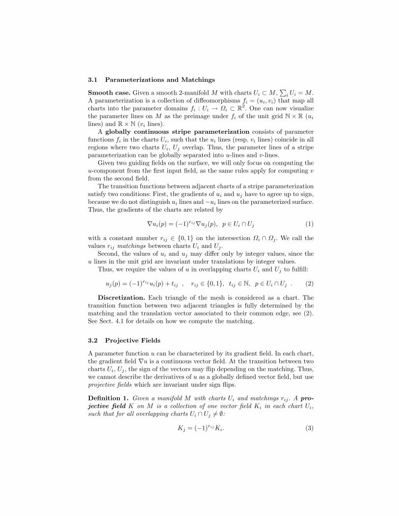
3.1 Parameterizations and Matchings

Smooth case. Given a smooth 2-manifold M with charts Ui ⊂M ,∑

i Ui = M .A parameterization is a collection of diffeomorphisms fi = (ui, vi) that map allcharts into the parameter domains fi : Ui → Ωi ⊂ R2. One can now visualizethe parameter lines on M as the preimage under fi of the unit grid N × R (ui

lines) and R× N (vi lines).A globally continuous stripe parameterization consists of parameter

functions fi in the charts Ui, such that the ui lines (resp. vi lines) coincide in allregions where two charts Ui, Uj overlap. Thus, the parameter lines of a stripeparameterization can be globally separated into u-lines and v-lines.

Given two guiding fields on the surface, we will only focus on computing theu-component from the first input field, as the same rules apply for computing vfrom the second field.

The transition functions between adjacent charts of a stripe parameterizationsatisfy two conditions: First, the gradients of ui and uj have to agree up to sign,because we do not distinguish ui lines and−ui lines on the parameterized surface.Thus, the gradients of the charts are related by

∇ui(p) = (−1)rij∇uj(p), p ∈ Ui ∩ Uj (1)

with a constant number rij ∈ 0, 1 on the intersection Ωi ∩ Ωj . We call thevalues rij matchings between charts Ui and Uj .

Second, the values of ui and uj may differ only by integer values, since theu lines in the unit grid are invariant under translations by integer values.

Thus, we require the values of u in overlapping charts Ui and Uj to fulfill:

uj(p) = (−1)rijui(p) + tij , rij ∈ 0, 1, tij ∈ N, p ∈ Ui ∩ Uj . (2)

Discretization. Each triangle of the mesh is considered as a chart. Thetransition function between two adjacent triangles is fully determined by thematching and the translation vector associated to their common edge, see (2).See Sect. 4.1 for details on how we compute the matching.

3.2 Projective Fields

A parameter function u can be characterized by its gradient field. In each chart,the gradient field ∇u is a continuous vector field. At the transition between twocharts Ui, Uj , the sign of the vectors may flip depending on the matching. Thus,we cannot describe the derivatives of u as a globally defined vector field, but useprojective fields which are invariant under sign flips.

Definition 1. Given a manifold M with charts Ui and matchings rij. A pro-jective field K on M is a collection of one vector field Ki in each chart Ui,such that for all overlapping charts Ui ∩ Uj 6= ∅:

Kj = (−1)rijKi. (3)

Discretization. The projective fields are piecewise constant on the triangles.Store one vector per triangle and the matching number on each edge. This fullydefines a discrete projective field. An odd matching at any edge means that thevector in one adjacent triangle corresponds to the negated vector of the othertriangle.

3.3 Branched Covering Spaces

We use the notion of branched covering surfaces for an equivalent descriptionof projective fields. A projective field on the input surface can be regarded as avector field on a covering surface. This allows us to apply standard vector fieldcalculus to projective fields.

Coverings. First, recall some definitions on Riemann surfaces, see [19–21].We will give an abstract definition of a covering and explain below how weactually construct one.

U ′i,0

U ′i,1

τ0i τ1

i

Ui

πi

πi πj

Ui Uj

U ′i,0

U ′i,1

U ′j,0

U ′j,1

πi πj

Ui Uj

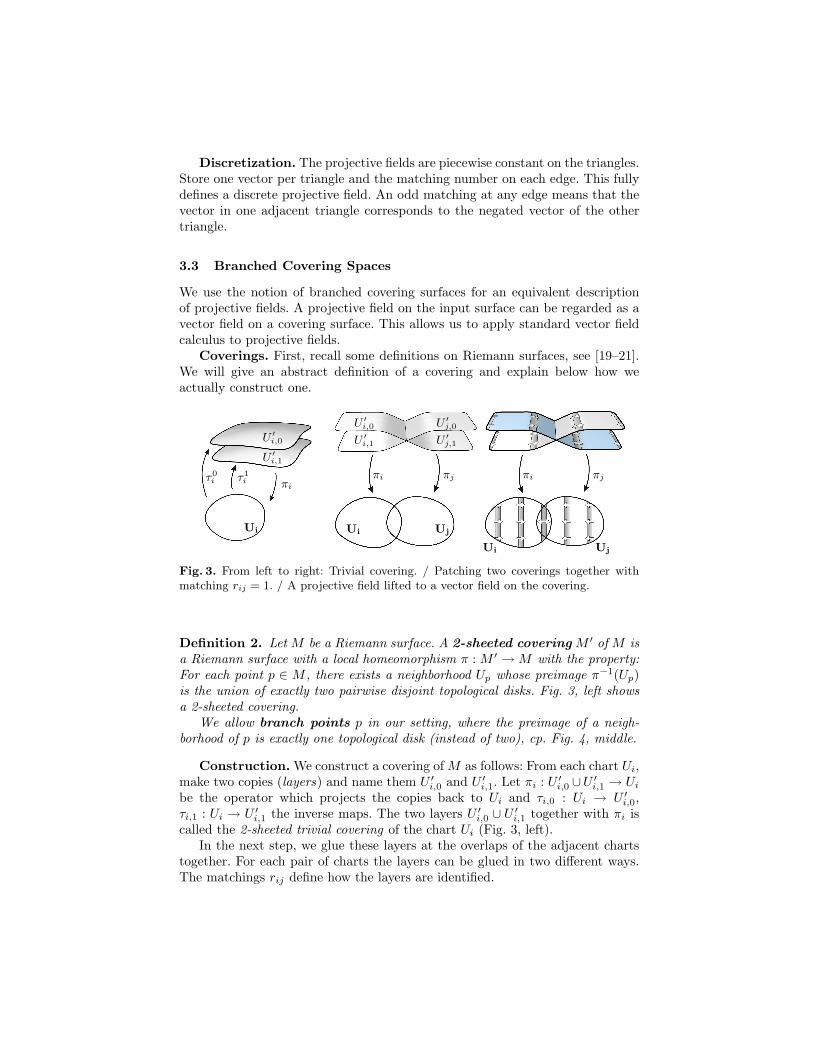
Fig. 3. From left to right: Trivial covering. / Patching two coverings together withmatching rij = 1. / A projective field lifted to a vector field on the covering.

Definition 2. Let M be a Riemann surface. A 2-sheeted covering M ′ of M isa Riemann surface with a local homeomorphism π : M ′ →M with the property:For each point p ∈ M , there exists a neighborhood Up whose preimage π−1(Up)is the union of exactly two pairwise disjoint topological disks. Fig. 3, left showsa 2-sheeted covering.

We allow branch points p in our setting, where the preimage of a neigh-borhood of p is exactly one topological disk (instead of two), cp. Fig. 4, middle.

Construction. We construct a covering of M as follows: From each chart Ui,make two copies (layers) and name them U ′i,0 and U ′i,1. Let πi : U ′i,0 ∪U ′i,1 → Ui

be the operator which projects the copies back to Ui and τi,0 : Ui → U ′i,0,τi,1 : Ui → U ′i,1 the inverse maps. The two layers U ′i,0 ∪ U ′i,1 together with πi iscalled the 2-sheeted trivial covering of the chart Ui (Fig. 3, left).

In the next step, we glue these layers at the overlaps of the adjacent chartstogether. For each pair of charts the layers can be glued in two different ways.The matchings rij define how the layers are identified.

Fig. 4. Left: Stripe parameterization with branch point. The isolines of the u functionand its gradient vectors are drawn. Middle: The same parameter function on the 2-sheeted covering (the covering surface is not embedded, it has self-intersections). Right:Branch point on a parameterized tube object.

Definition 3. A covering surface induced by matchings rij is uniquelydefined by the following construction:

Let (U ′i , πi) be 2-sheeted trivial coverings of the charts Ui. The covering sur-face is given as the union of all U ′i where the following points are identified: Ineach two overlapping charts Ui, Uj, identify all points τi,0(p) with τj,rij

(p) andτi,1(p) with τj,1−rij

(p), p ∈ Ui ∩ Uj (see Fig. 3, middle).

Since the trivial coverings of charts have no branch points and the chartscover the surface, we cannot construct any branch points this way. We allowbranch points by removing single points from the surface. Depending on thematchings we obtain a branch point there as shown in Fig. 3.

Discretization. In the discrete setting, branch points are located at vertices.On a 2-sheeted covering they occur when the sum of all matchings of incidentedges is odd. This means starting somewhere in the neighborhood of v andwalking once around the vertex ends on a different layer in the covering thanthe start point.

3.4 Vector Fields on Covering Spaces

Projective fields can be described as vector fields on a covering surface. Thisresult allows us to apply the classical vector field theory to projective fields.

A projective field K on M with matchings rij canonically lifts to a vectorfield K ′ on the covering induced by rij . In each chart Ui, define the vectors onits trivial covering as follows: For all p ∈ U ′i,0 set K ′(p) := Ki(πi(p)) and forp ∈ U ′i,1 set K(p) := −Ki(πi(p)), see Fig. 3, third image.

The result is a globally well defined vector field K ′ on M ′, since the layers ofthe covering are connected in the same way as the vector fields permute whenanother chart is chosen.

Definition 4. Let M be a manifold with matchings rij and M ′ the inducedcovering. A projective field lifted to a vector field K on M ′ is called a coveringfield of M .

4 Stripe Parameterizer Algorithm

In this section we describe the main extensions and simplifications which havebeen made to QuadCover to yield the stripe parameterizer. An important dif-ference is the use of projective vector fields instead of frame fields.

Compute the potential function. Given a surface M together with aprojective field K, or, equivalently, a covering surface M ′ with a vector field K ′.The parameter function is a scalar function u′ : M ′ → R. It can be projectedback to a parameter function u : M → R by taking the values of u′ in one of thetwo layers (it does not matter which layer is taken, because the parameter linesin both layers will be congruent).

The parameterization algorithm is divided into two stages: Assuring localcontinuity and global continuity. The two stages are explained in Sect. 4.3 and4.4. Sect. 4.1 deals on the creation of an input field. For the integration of aprojective field, we need to cut the surface open at a given cut graph. Sect. 4.2explains the construction of such a cut graph.

4.1 Generate Input Field and Matching

Curvature field. In our experiments, we used the field of minimum principlecurvatures as input to the parameterizer. Discrete principal curvature directionsand values can be calculated as proposed in [22] or [23]. Note that we deal withcurvatures given on triangles, not on vertices.

Finally, one gets a unit vector v in each triangle pointing in along that prin-ciple curvature direction which corresponds to the (absolute) smaller curvaturevalue. In triangle t, set K0(t) := v and K1(t) = −v.

We define matchings rij between every two adjacent triangles ti and tj bysetting rij = 0 if 〈K0(ti),K0(tj)〉 ≥ 0 and rij = 1 otherwise. This ensures thatthe field does not turn around, but proceeds as straight as possible.

Note that the position of branch points immediately follows from the choiceof matchings and the matchings are determined by the input field. A branchpoint arises at each vertex where the sum of matching of outgoing edges is odd.

4.2 Generating Cut Paths

A cut graph is a graphG embedded in the surface, such thatM\G is a topologicaldisk. We use a cut graph for the integration of projective fields in Sect. 4.3, anduse cut paths for the global continuity in Sect. 4.4.

Cut paths on M . Loosely speaking, cut paths are a set of paths on thesurface whose union is a cut graph. On closed surfaces, generating loops of thefirst fundamental group are suitable cut paths. In QuadCover, we use certaingenerators, namely the shortest system of loops as computed in Erickson andWhittlesey [24]. A system of loops is a set of 2g simple loops with a commonbase point, whose union is a cut graph.

We can treat branch points as tiny holes, as if they were removed fromthe surface (see Sect. 3.3). Erickson and Whittlesey handled closed surfaces

only, but we might have a surface with boundary. Once we have more thanone boundary component, each additional boundary component needs one path.Thus, in presence of b > 1 boundary components (or branch points) we need2g + b− 1 paths.

In our implementation for triangle

Fig. 5. Surface with boundary and twobranch points. The colored lines visualizethe five cut paths.

meshes we identify all boundary ver-tices and branch points into one pointB. On this surface (now without anyboundary), we apply the method of[24] with B as the base point. Whenwe undo the identification of bound-ary points, the paths which loopedthrough B now turn into paths thatconnect boundary components andbranch points.

Cut paths on covering. For ouralgorithm, we need cut paths on thecovering surface M ′. We get the cutpaths by computing them on M andlifting them to the covering. The resulting paths cut M ′ into two separate simplyconnected pieces. Thus, one of the paths could theoretically be discarded. It doesnot matter for our method that the covering decomposes into two pieces. It ismore important, that the cut paths are symmetric with respect to a change oflayers, i. e., for each path there is another path which runs in the other layerand has the same projection onto M , see Sect. 4.4.

4.3 Local Continuity

The gradient of the parameterization should align with the given input field aswell as possible, i. e., u′ should minimize the energy

E(u′) =∫

M ′

‖∇u′ −K ′‖2dA. (4)

Recall, that the vectors of K ′ are identical up to a different sign in the twolayers. Since the energy has a unique minimum and due to the symmetric shapeM ′, the solution u′ is also a map with negated function values in different layers.

The optimization problem (4) can be solved using the Hodge-Helmholtz de-composition. It states, that any vector field K ′ has a unique decomposition

K ′ = P + C +H (5)

with a gradient field P , a cogradient field C and a harmonic field H. P and Hare curl free (locally integrable), whereas C contains the curl part. Furthermore,the three spaces of potential fields, copotential fields and harmonic vector fieldsare perpendicular in L2 norm. Thus, discarding the second term leads to a curl

free field X ′ := P +H whose integral is the minimizer of Energy (4). The middleterm C of the Hodge-Helmholtz decomposition is a non-conforming functionand is found by solving a linear system of equations with one variable per edge.For details on the Hodge decomposition and integration of discrete vector fieldssee [25].

So far, the parameterization algorithm outlines as follows:

1. Perform Hodge-Helmholtz decomposition of input field K ′.2. Discard the non-integrable curl part and obtain a locally integrable field.3. Cut the surface open to be simply connected and lift the cut graph to the

covering, such that the covering is cut into two connected pieces.4. Obtain the parameterization u′ by integration: Perform a linear run over

all vertices (using a growing disk which does not cross the cut graph) andcompute the parameter values at each vertex such that the gradient matchesup with the vector field.

4.4 Global Continuity

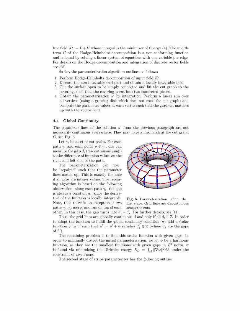
The parameter lines of the solution u′ from the previous paragraph are notnecessarily continuous everywhere. They may have a mismatch at the cut graphG, see Fig. 6.

Let γi be a set of cut paths. For each

Fig. 6. Parameterization after thefirst stage. Grid lines are discontinuousacross the cuts.

path γi and each point p ∈ γi, one canmeasure the gap di (discontinuous jump)as the difference of function values on theright and left side of the path.

The parameterization can nowbe ”repaired” such that the parameterlines match up. This is exactly the caseif all gaps are integer values. The repair-ing algorithm is based on the followingobservation: along each path γi, the gapis always a constant di, since the deriva-tive of the function is locally integrable.Note, that there is an exception if twopaths γi, γj merge and run on top of eachother. In this case, the gap turns into di + dj . For further details, see [11].

Thus, the grid lines are globally continuous if and only if all di ∈ Z. In orderto adapt the function to fulfill the global continuity condition, we add a scalarfunction ψ to u′ such that u′ := u′ + ψ satisfies d′j ∈ Z (where d′j are the gapsof u′).

The remaining problem is to find this scalar function with given gaps. Inorder to minimally distort the initial parameterization, we let ψ be a harmonicfunction, as they are the smallest functions with given gaps in L2 norm. ψis found via minimizing the Dirichlet energy ED =

∫M‖∇ψ‖2dA under the

constraint of given gaps.The second stage of stripe parameterizer has the following outline:

1. Compute cut paths γi.2. Measure gaps di.3. Find harmonic map ψ with gaps round(di)− di.4. Add ψ to u′.

In step 3, the gaps are rounded to the closest integer. Rounding the gapssuch that the distortion is minimized is an NP hard combinatorial problem. Aswe do not solve this problem exactly, the rounding behavior slightly depends onthe choice of cut paths.

5 Results

We have tested our method on different tube-like surfaces. Simple examplesare the knots in Fig. 7 without branchings. The principal curvature directionsare stable and can be computed very accurate in each point, so the algorithmproduces a parameterization of high quality.

Fig. 7. Left: Only u coordinates are used to map stripes on the knot surface. Middle:Only v coordinates are used. Right: u and v coordinates are used. The texture imageis a diagonal line which connects two opposite corners.

Fig. 8. The tree model of Fig. 1 with diagonal stripe pattern generates a candy cane.Singularities are marked in green.

The tree in Fig. 8 has a more complicated shape. It bifurcates and the thick-ness of the twigs vary. Note the accurate placement of branch points. There aretwo branch points at each bifurcation, allowing the circular stripes to split.

Fig. 10 shows a complex neuron model of genus 23, captured using confocalmicroscopy. The produced parameterization has very little distortion even onthis complicated object.

The unshaded version in the top demonstrates how a stripe pattern helpsto perceive the complicated shape of the neuron. But also in the fully shadedimages, the stripes help to capture the object more easily.

The surface in Fig. 9 shows a human blood vessel which contains parts witha very large tube radius as well as very filigrane branches. Regardless of thisdifference in the scaling, the stripe density stays nearly constant everywhere.

Fig. 9. Parameterized blood vessel, captured by MRT. Courtesy of Fraunhofer MEVIS.

The parameterization of these models was fully automatic. We only chose thedensity of the lines and the amount of curvature field smoothing. The modelshad approximately 20k to 40k triangles and the algorithm terminated in lessthan a minute.

6 Acknowledgements

The authors are grateful to Christian Hansen of Fraunhofer MEVIS (Bremen,Germany) for providing clinical 3D models of vascular structures and fruitfuldiscussions concerning this work.

Many thanks to Sabine Krofczik and Jurgen Rybak, Department of Neuro-biology at Freie Universitat Berlin, as well as Steffen Prohaska and Anja Ku,Zuse Institute Berlin (ZIB) for supplying the neuron geometry.

This research was supported by the DFG Research Center MATHEON andby mental images.

Fig. 10. Parameterized neuron by courtesy of Freie Universitat Berlin, Department ofNeurobiology. Top: depth shading. Bottom: full shading.

References

1. Floater, M.S., Hormann, K.: Surface parameterization: a tutorial and survey. InDodgson, N.A., Floater, M.S., Sabin, M.A., eds.: Advances in multiresolution forgeometric modelling. Springer Verlag (2005) 157–186

2. Hormann, K., Polthier, K., Sheffer, A.: Mesh parameterization: Theory and prac-tice. In: SIGGRAPH Asia 2008, Course Notes. Number 11 (2008)

3. Tutte, W.T.: How to draw a graph. Proc. London Math. Soc. s3-13(1) (1963)743–767

4. Haker, S., Angenent, S., Tannenbaum, A., Kikinis, R., Sapiro, G., Halle, M.: Con-formal surface parameterization for texture mapping. IEEE Trans. on Visualizationand Computer Graphics 6(2) (2000) 181–189

5. Gu, X., Yau, S.T.: Global conformal surface parameterization. In: Symp. on Geom.Proc. (2003) 127–137

6. Jin, M., Wang, Y., Yau, S.T., Gu, X.: Optimal global conformal surface parame-terization. In: In IEEE Visualization. (2004) 267–274

7. Kharevych, L., Springborn, B., Schroder, P.: Discrete conformal mappings viacircle patterns. ACM Trans. on Graphics 25(2) (2006)

8. Tong, Y., Alliez, P., Cohen-Steiner, D., Desbrun, M.: Designing quadrangulationswith discrete harmonic forms. In: Eurographics Symp. on Geom. Proc. (2006)

9. Dong, S., Bremer, P.T., Garland, M., Pascucci, V., Hart, J.: Spectral surfacequadrangulation. ACM SIGGRAPH (2006)

10. Ray, N., Li, W.C., Levy, B., Sheffer, A., Alliez, P.: Periodic global parameterization.ACM Trans. Graph. 25(4) (2006) 1460–1485

11. Kalberer, F., Nieser, M., Polthier, K.: Quadcover - surface parameterization usingbranched coverings. Comput. Graph. Forum 26(3) (2007) 375–384

12. Ray, N., Vallet, B., Li, W.C., Levy, B.: N-symmetry direction field design. ACMTrans. Graph. 27(2) (2008) 1–13

13. Palacios, J., Zhang, E.: Rotational symmetry field design on surfaces. ACM Trans.on Graphics 26(3) (2007) 55:1–55

14. Zhang, E., Hays, J., Turk, G.: Interactive Tensor Field Design and Visualizationon Surfaces. IEEE Trans. on Visualization and Computer Graphics (2007) 94–107

15. Lai, Y.K., Jin, M., Xie, X., He, Y., Palacios, J., Zhang, E., Hu, S.M., Gu, X.D.:Metric-driven rosy fields design. Technical report, Tsinghua Univ., Beijing (2008)

16. Huysmans, T., Sijbers, J., Verdonk, B.: Parametrization of tubular surfaces on thecylinder. In: WSCG (Journal Papers). (2005) 97–104

17. Antiga, L., Steinman, D.: Robust and objective decomposition and mapping ofbifurcating vessels. IEEE Trans. on Medical Imaging 23(6) (2004) 704–713

18. Zhu, L., Haker, S., Tannenbaum, A.: Flattening maps for the visualization ofmulti-branched vessels (2005)

19. Farkas, H.M., Kra, I.: Riemann Surfaces. Springer Verlag (1980)20. Fulton, W.: Algebraic Topology, A first course. Springer Verlag (1995)21. Jost, J.: Compact Riemann Surfaces. Springer (2002)22. Cohen-Steiner, D., Morvan, J.M.: Restricted delaunay triangulations and normal

cycle. In: Proc. of Symp. on Comp. Geom., ACM Press (2003) 312–32123. Hildebrandt, K., Polthier, K.: Anisotropic filtering of non-linear surface features.

Computer Graphics Forum 23(3) (2004) 391–40024. Erickson, J., Whittlesey, K.: Greedy optimal homotopy and homology generators.

In: Proc. 16th ACM-SIAM Symp. on Discrete Algorithms. (2005) 1038–104625. Polthier, K., Preuss, E.: Identifying vector field singularities using a discrete Hodge

decomposition. In: Visualization and Mathematics III. Springer (2003) 113–13426. Praun, E., Hoppe, H., Webb, M., Finkelstein, A.: Real-time hatching. In: SIG-

GRAPH. (2001) 58127. Zockler, M., Stalling, D., Hege, H.C.: Fast and intuitive generation of geometric

shape transitions. The Visual Computer 16(5) (2000) 241–253